Embed Size (px)
Citation preview

Indoor Navigation and Manipulation using a Segway RMP
May 1, 2014
Submitted to:
Project Advisor: Prof. Gregory S. Fischer Project Co-Advisor: Asst. Prof. Dmitry Berenson
A Major Qualifying Project submitted to the Faculty of Worcester Polytechnic Institute in partial fulfillment of the requirements for the degree of Bachelor of
Science.
Submitted by:
Christopher Dunkers Brian Hetherman Paul Monahan Samuel Naseef

Abstract The goal of this project was to work with a Segway RMP, utilizing it in an assistive-
technology manner. This encompassed navigation and manipulation aspects of robotics. First,
background research was conducted to develop a blueprint for the robot. The hardware,
software, and configuration of the given RMP were updated, and a robotic arm was designed to
extend the platform’s capabilities. The robot was programmed to accomplish semi-autonomous
multi-floor navigation through the use of the navigation stack in ROS (Robot Operating System),
image detection, and a user interface. The robot can navigate through the hallways of the
building, using the elevator to travel between floors. The robotic arm was designed to
accomplish basic tasks, such as pressing a button and picking an object up off of a table. The
Segway RMP is designed to be utilized and expanded upon as a robotics research platform.
i

Executive Summary Our team planned to enable the Segway platform to be utilized in an assistive
technology manner. We proposed the mobile platform could be used in a manner that could aid bedridden patients in fetching items around a house, eliminating the need for nurses or aides to be present at home full time. The main goal of our project was to create a research platform with the capability of navigating autonomously to a position in a multi-floor building designated by a user.
First, background research was conducted on existing mobile manipulation and assistive technology platforms and the technical specifications of the subsystems involved with these systems. We found some trends and discovered potential problem areas surrounding navigation and manipulation.
Moving forward, the platform was programmed to navigate multi-floor indoor facilities, given basic floor plans, while also designing, building, and implementing a robotic manipulator. To start, the RMP first had to be disassembled and updated.
Figure 1: Original control box (Left) and new control box (right)
The power distribution created by the previous MQP was altered, given the new sensors
and arm that would be built. The physical setup was updated from terminal blocks to a printed circuit board, which made cabling a lot cleaner and easier to change.
Figure 2: Original terminal block power distribution (left) and new PCB power distribution board (right)
A robotic manipulator was designed and built to achieve the goals set out by the team,
which included reaching a height ranging from 30” to 60” off the floor, extending 2’ from the
ii

edge of the robot and being able to lift an object the size of a Nalgene bottle, weighing up to a couple pounds.
Figure 3: Side view (left) and top view (right) of the final arm design
The base platform had its code-base updated from the previous MQP and some basic
scripts were written to assist in the start-up of the platform. From there, several navigation and image processing stacks in ROS were implemented on the platform. Here you can see the occupancy grid and other visualizations in ROS of the floor plan and the sensed environment.
Figure 4: ROS visualization during navigation and obstacle avoidance
Overall, the platform performed well given the limitations. There were several issues
encountered including the computer not being powerful enough. While running the navigation stacks and the visualizations, all four processing cores were at full capacity. This prevented using multiple subsystems at the same time, like arm kinematic calculations and object detection. Although these abilities did not get implemented, these problems would be anticipated.
Additional issues come into play with the physical design of the manipulator. Given the small budget, we had to make compromises on some of the design details, like having bearings for the rotation joints. Having actual bearings would give the joints more stability and make them less likely to deform and wear during operation.
iii

Acknowledgments We would like to thank the following individuals and organizations for their support and
contribution to the success of this project:
• Chris Crimmins and Segway, Inc. for the donation and continued support of the
Segway RMP 200
• Dr. GregoryFischer for being an advisor and donating AIM Lab space and
resources to our project.
• Joe St. Germain for his continued support and advice, and for lending the LIDAR
sensor to our project.
iv

Contributions & Authorship Christopher Dunkers: Chris was primarily responsible for the electrical layout of the robot, PCB design. High level (ROS) software for both the navigation and the arm, navigation user interface, template matching using the kinect for navigation, sensor integration, ROS catkinization, ROS workspace structure, ROS package integration, Segway interface in ROS. Author or co-author of Technical Review sections 3.7 Mobile Navigtion and 3.9 Object Recognition; Methodology sections 4.1 Robot Design Overview and 4.4 Software; Results sections 5.1 Electrical Design and 5.3 Navigation; Discussion sections 6.1 Electrical Design and 6.3 Navigation and Software; and the Conclusions and Recommendations section.
Brian Hetherman: Brian was primarily responsible for the designing the layout of the hardware on the Segway RMP platform, sensor integration, creation of bitmaps used for navigation, navigation graphical user interface, all software that controlled navigation, software for template matching using the Kinect sensor and assisted with design, assembly and sensor integration for the mechanical arm. Author or co-author of Technical Review sections 3.4 Stereo Vision, 3.5 Scanning Laser Rangefinder and 3.6 Occupancy Grids; Methodology section 4.4 Software; Results section 5.3 Navigation; Discussion section 6.3 Navigation and Software; Appendix C: Arm Control Code; and Conclusions and Recommendations.
Paul Monahan: Paul was primarily responsible for the control logic of the manipulator, research and selection of the electronic hardware of the manipulator, some manufacturing and assembly, as well as being the point of contact with Segway and other purchasing orders. Author or co-author of Executive Summary; Introduction; Literature Review sections 2.2 Care-O-bot, 2.3 PR2, 2.4 KUKA youBot, 2.6 Literature Conclusions; Technical Review section 3.8 GUI Design; Methodology section 4.3 Arm Control; Results section 5.2 Arm Design and Construction; Discussion section 6.2 Arm Design & Control; and Conclusions and Recommendations.
Samuel Naseef: Samuel was primarily responsible for the iterative design, mechanical finite element analysis, fabrication, and assembly of the mechanical arm. Author or co-author of Literature Review sections 2.1 Mobile Manipulation and 2.5 Rollin’ Justin; Technical Review sections 3.1 Definition of the robotic arm, 3.2 Arm Design, and 3.3 Arm Kinematics; Methodology section 4.2 Arm Design; Results section 5.2 Arm Design and Construction; Discussion section 6.2 Arm Design & Control; and Appendix A: SolidWorks SimulationXpress Results. Samuel was also responsible for the maintenance of the team’s EndNote, and the formatting and editing of this paper.
v

Table of Contents ABSTRACT ............................................................................................................................................................... I
EXECUTIVE SUMMARY ........................................................................................................................................... II
ACKNOWLEDGMENTS ........................................................................................................................................... IV
CONTRIBUTIONS & AUTHORSHIP........................................................................................................................... V
TABLE OF CONTENTS ............................................................................................................................................. VI
TABLE OF FIGURES .............................................................................................................................................. VIII
TABLE OF TABLES ................................................................................................................................................... X
1.0 INTRODUCTION ................................................................................................................................................ 1
2.0 LITERATURE REVIEW ........................................................................................................................................ 2
2.1 MOBILE MANIPULATION ........................................................................................................................................... 2 2.2 CARE-O-BOT ........................................................................................................................................................... 4 2.3 PR2 ...................................................................................................................................................................... 6 2.4 KUKA YOUBOT ....................................................................................................................................................... 7 2.5 ROLLIN’ JUSTIN ........................................................................................................................................................ 8 2.6 LITERATURE CONCLUSIONS....................................................................................................................................... 10
3.0 TECHNICAL REVIEW ........................................................................................................................................ 11
3.1 DEFINITION OF THE ROBOTIC ARM ............................................................................................................................. 11 3.2 ARM DESIGN ......................................................................................................................................................... 12 3.3 ARM KINEMATICS .................................................................................................................................................. 13
3.3.1 Cartesian / Gantry Robot .......................................................................................................................... 14 3.3.2 Cylindrical Robot ....................................................................................................................................... 15 3.3.3 Spherical/Polar Robot ............................................................................................................................... 16 3.3.4 SCARA (Selective Compliance Assembly Robot Arm) Robot ...................................................................... 16 3.3.5 Articulated Robot ...................................................................................................................................... 17
3.4 STEREO VISION ...................................................................................................................................................... 17 3.5 SCANNING LASER RANGEFINDER ............................................................................................................................... 20 3.6 OCCUPANCY GRIDS ................................................................................................................................................ 21 3.7 MOBILE NAVIGATION ............................................................................................................................................. 23 3.8 GUI DESIGN ......................................................................................................................................................... 29 3.9 OBJECT RECOGNITION ............................................................................................................................................. 32
4.0 METHODOLOGY ............................................................................................................................................. 34
4.1 ROBOT DESIGN OVERVIEW ...................................................................................................................................... 34 4.2 ARM DESIGN ......................................................................................................................................................... 39
4.2.1 Arm Concept 1 - Rack & Pinion .................................................................................................................. 40 4.2.2 Arm Concept 2 - Lead Screw ...................................................................................................................... 40 4.2.3 Arm Concept 3 - Linkage ........................................................................................................................... 41 4.2.4 Linkage Design Iterations .......................................................................................................................... 42 4.2.5 Linkage Analysis ........................................................................................................................................ 45 4.2.6 Arm Analysis and Forward Kinematics ...................................................................................................... 47 4.2.7 Inverse Kinematics ..................................................................................................................................... 49
4.3 ARM CONTROL ...................................................................................................................................................... 51 4.3.1 Hardware .................................................................................................................................................. 51 4.3.2 Communication ......................................................................................................................................... 55
vi

4.3.3 Control ....................................................................................................................................................... 57 4.4 SOFTWARE ............................................................................................................................................................ 59
4.4.1 Map Publishers .......................................................................................................................................... 59 4.4.2 Sensors ...................................................................................................................................................... 62 4.4.3 Transforms and Frames ............................................................................................................................. 66 4.4.4 User Interface ............................................................................................................................................ 69 4.4.5 Segway Communication ............................................................................................................................ 70 4.4.6 Navigation ................................................................................................................................................. 71
5.0 RESULTS ......................................................................................................................................................... 74
5.1 ELECTRICAL DESIGN ............................................................................................................................................ 75 5.2 ARM DESIGN AND CONSTRUCTION ............................................................................................................................ 78 5.3 NAVIGATION ......................................................................................................................................................... 79
6.0 DISCUSSION ................................................................................................................................................... 84
6.1 ELECTRICAL DESIGN ................................................................................................................................................ 84 6.2 ARM DESIGN & CONTROL ........................................................................................................................................ 85 6.3 NAVIGATION AND SOFTWARE ................................................................................................................................... 86
7.0 CONCLUSIONS AND RECOMMENDATIONS ..................................................................................................... 91
REFERENCES ......................................................................................................................................................... 94
APPENDIX A: SOLIDWORKS SIMULATIONXPRESS RESULTS .................................................................................. 97
APPENDIX B: LAUNCH FILE ................................................................................................................................. 125
APPENDIX C: ARM CONTROL CODE .................................................................................................................... 126
vii

Table of Figures FIGURE 1: ORIGINAL CONTROL BOX (LEFT) AND NEW CONTROL BOX (RIGHT) ................................................................................ II FIGURE 2: ORIGINAL TERMINAL BLOCK POWER DISTRIBUTION (LEFT) AND NEW PCB POWER DISTRIBUTION BOARD (RIGHT) .................. II FIGURE 3: SIDE VIEW (LEFT) AND TOP VIEW (RIGHT) OF THE FINAL ARM DESIGN ........................................................................... III FIGURE 4: ROS VISUALIZATION DURING NAVIGATION AND OBSTACLE AVOIDANCE ........................................................................ III FIGURE 5: PLANAR MANIPULATOR MOUNTED ON A MOBILE PLATFORM (BAYLE ET AL., 2003) ......................................................... 4 FIGURE 6: CARE-O-BOT 3, DISPLAYING ITS ADJUSTABLE TRAY AND ROBOTIC ARM (AUTOMATION, 2013) ......................................... 5 FIGURE 7: FRONT VIEW OF PR2 WITH MULTITUDE OF SENSORS (GARAGE, 2014) ......................................................................... 6 FIGURE 8: KUKA'S YOUBOT (KUKA, 2013) .......................................................................................................................... 7 FIGURE 9: ROLLIN’ JUSTIN (BORST ET AL., 2009) .................................................................................................................... 9 FIGURE 10: KINEMATIC PAIRS WITH ASSOCIATED DEGREES OF FREEDOM (BEARDMORE, 2011) ..................................................... 14 FIGURE 11: CARTESIAN/GANTRY ROBOT (ROBOTS, 2013) ..................................................................................................... 15 FIGURE 12: CYLINDRICAL ROBOT (ROBOTS, 2013) ................................................................................................................ 15 FIGURE 13: SPHERICAL/POLAR ROBOT (ROBOTS, 2013) ........................................................................................................ 16 FIGURE 14: SCARA ROBOT (ROBOTS, 2013) ....................................................................................................................... 17 FIGURE 15: (ROBOTS, 2013) ............................................................................................................................................. 17 FIGURE 16: EPIPOLAR RECTIFICATION (MIRAN & MISLAV, 2010) ........................................................................................... 18 FIGURE 17: IMAGES FROM EACH CAMERA AFTER RECTIFICATION (GERIG, 2012) ......................................................................... 18 FIGURE 18: HOKUYO URG-04LX-UG01 SCANNING LASER RANGE FINDER (HOKUYO, 2009) ..................................................... 21 FIGURE 19: SHOWS IMAGE OF A SCENE (LEFT), RESULT OF MAPPING THE SCENE TO AND OCCUPANCY GRID (LEFT CENTER), RESULT OF
MAPPING THE SCENE TO QUADTREE OCCUPANCY GRID (CENTER RIGHT), AND ENLARGED COMPARISON OF OBJECTS IN THE MAPS (RIGHT) (LI & RUICHEK, 2013) ................................................................................................................................. 22
FIGURE 20: SIMPLE APPROACH TO THE SLAM PROBLEM (RIISGAARD & BLAS, 2003) ................................................................. 24 FIGURE 21: CORRIDOR CLASSIFICATION FOR A TOPOLOGICAL MAP (CORREA ET AL., 2012) ........................................................... 25 FIGURE 22: AN EXAMPLE TOPOLOGICAL MAP (CORREA ET AL., 2012) ....................................................................................... 26 FIGURE 23: FOCUSED D* MAP (STENTZ, 1995) .................................................................................................................... 28 FIGURE 24: SHOWS THE ARCHITECTURE FOR A MODEL/VIEW/CONTROLLER PATTERN. ................................................................ 30 FIGURE 25: ORIGINAL ROBOT OVERVIEW (LEBLANC, PATEL, & RASHID, 2012) .......................................................................... 34 FIGURE 26: PICTURE OF THE REAR OF THE ROBOT AT THE BEGINNING OF THE MQP ..................................................................... 35 FIGURE 27: PICTURE OF THE FRONT OF THE ROBOT AT BEGINNING OF MQP .............................................................................. 35 FIGURE 28: SEGWAY CONTROL BOX BEFORE SERVICING ........................................................................................................... 36 FIGURE 29: SEGWAY CONTROL BOX AFTER SERVICING ............................................................................................................ 36 FIGURE 30: ORIGINAL ELECTRICAL SCHEMATIC (LEBLANC, PATEL, & RASHID, 2012) .................................................................. 37 FIGURE 31: PROPOSED ELECTRICAL SCHEMATIC UPDATE .......................................................................................................... 37 FIGURE 32: ORIGINAL POWER DISTRIBUTION BOARD ............................................................................................................. 38 FIGURE 33: ARM CONCEPT 2 - RACK & PINION DESIGN (CORPERATION, 2012) .......................................................................... 40 FIGURE 34: ARM CONCEPT 3 - LEAD SCREW DESIGN (LIPSETT, 2013) ........................................................................................ 41 FIGURE 35: ARM CONCEPT 1 – LINKAGE DESIGN (CORPERATION, 2012) ................................................................................... 41 FIGURE 36: STRESS DIAGRAM FROM SOLIDWORKS FEA ......................................................................................................... 44 FIGURE 37: COMPLETED SOLIDWORKS ARM DESIGN (CORPERATION, 2012) ............................................................................. 44 FIGURE 38: LINKAGE DIAGRAM .......................................................................................................................................... 46 FIGURE 39: KINEMATIC DIAGRAM ....................................................................................................................................... 47 FIGURE 40: ELBOW DOWN (A) AND ELBOW UP (B) SOLUTIONS TO THE ARM INVERSE KINEMATICS (COMPUTING, 2013) ................... 51 FIGURE 41: MANIPULATOR DESIGN ..................................................................................................................................... 52 FIGURE 42: ARDUINO AND MOTOR DRIVERS MOUNTED ONTO THE ARM ASSEMBLY ...................................................................... 54 FIGURE 43: BYTE STRUCTURE FOR COMMUNICATION TO AND FROM THE ARDUINO...................................................................... 56 FIGURE 44: BASIC PID CONTROL FLOW ................................................................................................................................ 57 FIGURE 45: PID ORDER OF OPERATION ................................................................................................................................ 58 FIGURE 46: ORIGINAL FLOOR PLAN (LEFT) AND FINAL MODIFIED VERSION (RIGHT) FOR THE GROUND FLOOR OF A BUILDING. .............. 60 FIGURE 47: RVIZ MESSAGE VISUALIZATION ........................................................................................................................... 61
viii

FIGURE 48: LASER SCAN INFLATED FOR THE COST MAPS AS THE ROBOT IS TRAVELLING DOWN A HALLWAY ........................................ 64 FIGURE 49: KINECT POSITIVE RECOGNITION OF THE SECOND FLOOR FROM THE LED SCREEN IN THE ELEVATOR (LEFT) AND SCENE FROM
NON-KINECT CAMERA (RIGHT) .................................................................................................................................. 65 FIGURE 50: NAVIGATION TRANSFORMATION TREE ................................................................................................................. 67 FIGURE 51: RVIZ WITH PLANNED PATH, COST MAP, ROBOT POSE, AND LASER SCAN DATA ............................................................. 69 FIGURE 52: NAVIGATION STACK SETUP ................................................................................................................................ 71 FIGURE 53: MULTI-FLOOR PLANNER ELEVATOR PROTOCOL FLOW-CHART ................................................................................... 73 FIGURE 54: FINAL RESULT OF OUR ROBOT MODIFICATIONS ...................................................................................................... 74 FIGURE 55: FINAL POWER DISTRIBUTION SCHEMATIC ............................................................................................................. 75 FIGURE 56: CONNECTORS USED ON THE POWER DISTRIBUTION PCB (PRODUCTS, 2014) ............................................................. 76 FIGURE 57: POWER DISTRIBUTION PCB (ALTIUM, 2014) ...................................................................................................... 77 FIGURE 58: FINAL COMMUNICATION SCHEMATIC .................................................................................................................. 77 FIGURE 59: ARM FINAL DESIGN (SIDE VIEW OF LINKAGE) ......................................................................................................... 79 FIGURE 60: ARM FINAL DESIGN (TOP VIEW OF PLANAR ARM) ................................................................................................... 79 FIGURE 61: ROS SCHEMATIC FOR THE ROBOT WHEN NAVIGATING ............................................................................................ 80 FIGURE 62: NAVIGATION RQT PLUGIN (GROUND FLOOR) ........................................................................................................ 81 FIGURE 63: NAVIGATION RQT PLUGIN (FIRST FLOOR) ............................................................................................................. 82 FIGURE 64: ROBOT WITH CLEAR PATH.................................................................................................................................. 83 FIGURE 65: ROBOT WITH OBSTACLE IN PATH ......................................................................................................................... 83 FIGURE 66: ROBOT WITH NEW PATH AROUND OBSTACLE ........................................................................................................ 83 FIGURE 67: SYSTEM MONITOR WHILE THE ROBOT WAS NAVIGATING ......................................................................................... 87 FIGURE 68: SOLIDWORKS SIMULATION OF COUPLER HORIZONTAL LINKAGE MOUNT (CORPERATION, 2012) .................................. 103 FIGURE 69: SOLIDWORKS SIMULATION OF FINAL ARM LINK 1 (CORPERATION, 2012) ............................................................... 110 FIGURE 70: SOLIDWORKS SIMULATION OF T-SLOTTED EXTRUSION 5IN (CORPERATION, 2012) ................................................... 117 FIGURE 71: SOLIDWORKS SIMULATION OF WRIST 3.0 (CORPERATION, 2012) ......................................................................... 124
ix

Table of Tables TABLE 1: DEGREES OF FREEDOM IN THE UPPER BODY OF THE ROLLIN’ JUSTIN PLATFORM (BORST ET AL., 2009) ................................. 9 TABLE 2: RESULTS FROM THE EXECUTION OF FOUR DIFFERENT ALGORITHMS (STENTZ, 1995) ........................................................ 27 TABLE 3: DENAVIT–HARTENBERG TABLE .............................................................................................................................. 48 TABLE 4: POLOLU MOTOR DRIVER PERFORMANCE SPECIFICATIONS ............................................................................................ 53 TABLE 5: CIM MOTOR PERFORMANCE SPECIFICATIONS ........................................................................................................... 53 TABLE 6: VEX SERVO PIN LAYOUT ........................................................................................................................................ 55 TABLE 7: CANAKIT MOTOR DRIVER CONTROL PIN LAYOUT ........................................................................................................ 55 TABLE 8: POLOLU MOTOR DRIVER CONTROL PIN LAYOUT ......................................................................................................... 55
x

1.0 Introduction The purpose of this project was to develop the Segway RMP200 platform into an
assistive technology. The hope was to create a platform that could empower disabled people to
live full, independent lives by being able to complete basic object retrieval tasks or even act as
telepresence for the user. An alternative use of the platform could be in a hospital setting in
retrieving supplies for nurses. Therefore, the main goal of this project is to develop a research
platform capable of autonomously navigating multi-floor facilities and retrieving objects for
users.
Existing assistive technologies were explored for common themes to emulate in the
system being developed. The subsystems of assistive technologies and mobile manipulation
platforms were examined in greater detail to gain a better understanding of how to execute a
solution.
Once there was a clear understanding of the problem and how to implement a solution,
different algorithms and mechanical designs were explored. They were compared against each
other before deciding upon the team’s approach. The solution was executed and analyzed
along the way. The results of the solution are discussed at length and recommendations for the
future were generated based on the progress made during this project.
1

2.0 Literature Review In order to fully understand the goals of our project we looked at other robots that have
been developed for the similar purposes. In the sections that follow we look critically at robots
that were designed as assistive mobile robots. We will examine the capabilities of the various
robots and how they function. From this review we hope to gain knowledge that will help
inform which properties are most valuable for assistive mobile robots which we can then
incorporate into our own robot design.
2.1 Mobile Manipulation A robot designed as a human “assistant” must be able to interact with the environment;
grabbing, pushing, lifting, and manipulating objects, while maneuvering to reach, avoid
collision, and navigate through its workspace. In addition to the complex kinematic
coordination this involves, a full integration of both mobility and manipulation must also
address the interactions between these two dynamic systems. Mobile manipulation systems
combine the advantages of mobile platforms and robotic arms while reducing their drawbacks
by extending the robots workspace and operational functionalities (Bayle, Fourquet, & Renaud,
2003).
For wheeled mobile platforms, rolling without slipping, or RWS, of the wheels on the
ground introduces unique difficulties in the kinematic modeling of the system. The mobile base,
which isn’t capable of instantaneous motion in any arbitrary direction, is therefore said to be a
nonholonomic system. The wheels of a mobile platform can be classified into four categories:
fixed wheels, steered wheels, castor wheels, and Swedish wheels.
2

• Fixed wheels, for which the axle has a fixed direction;
• Steered wheels, for which the wheel can be mechanically steered and the orientation
axis passes through the center of the wheel;
• Castor wheels, for which the wheel isn’t driven and the orientation axis does not pass
through the center of the wheel;
• Swedish wheels, which are similar to fixed wheels, with the exception of an additional
parameter that describes the direction, with respect to the wheel plane, of the zero
component of the velocity at the contact point (Bayle et al., 2003).
“Manipulability of Wheeled Mobile Manipulators: Application to Motion Generation” is
a journal article from The International Journal of Robotics Research focusing on the modeling
of nonholonomic mobile manipulators, which are made up of a robotic arm mounted on a
wheeled mobile platform. Figure 5 below gives an example of the generic modeling of the
mobile manipulator, which is analyzed in the paper (Bayle et al., 2003).
3

Figure 5: Planar manipulator mounted on a mobile platform (Bayle et al., 2003)
The analysis performed in the paper is extremely detailed, and provides an in depth,
broken-down example of the manipulability, mobile control strategy, and motion planning
problem for mobile manipulation platforms. This will provide a guide for the creation of the
control strategies for mobile manipulation, which we unfortunately did not have the
opportunity to implement.
2.2 Care-O-bot Care-O-bot 3 was developed by the Fraunhofer Institute for Manufacturing Engineering
and Automation. The goal was to design a robotic home assistant that was robust and flexible,
very similar to the task here.
4

Figure 6: Care-O-bot 3, displaying its adjustable tray and robotic arm (Automation, 2013)
The institute developed this product for over 15 years as a robot to “actively assist
humans in their day-to-day lives”(Automation, 2013). This third generation of the robot is a
pinnacle of mobile manipulations. The robot sits on 4 steered and driven wheels and has a
seven DoF arm, with a three finger gripper. The fingers have tactile sensors to monitor the
pressure being applied by the gripper. The robot itself has a vast array of sensors to fully define
a 3D environment and uses them to avoid obstacles, static and dynamic. Given its functionality,
this robot is capable of navigating autonomously and retrieving objects with ease. It is even
coordinated enough to open any door in its path.
The software used to develop this platform was ROS and all of its code and simulation
information is given online. The platform has been developed to be put into use as well as serve
as a research platform.
5

In comparison to the goal of this project, this robot goes above and beyond the
specifications set out by the team. The company spent 15 years developing this platform and
had the resources to create a robot that is extremely robust and flexible for any environment.
The Care-O-bot would be a platform to imitate in functionality and execution; the hardware
and development are outside the scope of this project simply because the budget and time
span of this project are serious constraints (Graf, Hans, & Schraft, 2004).
2.3 PR2 The PR2 is an omni-directional, two-armed mobile platform developed by Willow
Garage as a research platform. It contains a multitude of degrees of freedom and is robust
enough to manipulate any everyday object. The manipulators were designed to provide high
torque but remain flexible enough to operate in unknown environments. The platform comes
with a suite of sensors including multiple LIDAR and stereoscopic cameras.
Figure 7: Front view of PR2 with multitude of sensors (Garage, 2014)
This platform has more capabilities than could be achieved in the timeframe and budget
of this project. The sensors and hardware on this system are expensive when compared to the
budget we are working with, but the design of the manipulators are to be admired. The design
6

makes use of several cameras to fully sense an object, which makes object recognition more
reliable. This also increases the computation needed on the platform. Realistically, developing
as robust manipulators and developing the platform as a whole would require a lot more
resources and time than we have available (Garage, 2014).
2.4 KUKA youBot A major qualifying project conducted on WPI’s campus revolved around the KUKA
youBot platform. The youBot is a small mobile platform with omni-directional wheels and a 5-
DoF arm. On the platform, a Kinect was mounted and cameras were mounted above the
environment. The project was completed under the Robot Autonomy and Interactive Learning
Lab (RAIL), whose lab goal is to provide web-based control of the youBot. The project explored
the ability of the platform to operate in a small environment with furniture and an assortment
of objects (Jenkel, Kelly, & Shepanski, 2013).
Figure 8: KUKA's youBot (KUKA, 2013)
7

The project explored the platform’s mechanical and software abilities within the existing
ROS stacks but found that there was no stack that suited their needs. As a result, they
developed their own ROS stack to satisfy their goals (Jenkel et al., 2013).
Overall, this project gives us an insight into ROS development for our project. The team
didn’t have to design and build a manipulator, and were able to strictly focus on algorithm
development and integration. And given that this project was conducted on the same campus,
we can make use of these professors as resources during our own progress.
2.5 Rollin’ Justin Rollin’ Justin is a mobile humanoid robotic system designed as a research platform for
use in servicing tasks by The German Aerospace Center’s Institute of Robotics and Mechatronics
in Oberpfaffenhofen. Rollin’ Justin” is a mobile robotic system that allows sophisticated control
algorithms for complex kinematic chains, dexterous two handed manipulation, and navigation
while in typical human environments. In designing the platform, special emphasis was placed
on mechanical design features, control issues, and high-level system capabilities such as human
robot interaction (Borst et al., 2009).
8

Figure 9: Rollin’ Justin (Borst et al., 2009)
The Rollin’ Justin platform is extremely intricate, including 43 degrees of freedom in the
upper body as detailed in Table 1. The platform is capable of safely interacting directly with
humans, making it an excellent model for future research in assistive robotic technologies.
Subsystem Torso Arms Hands Head & Neck Σ DoF 3 2 x 7 2 x 12 3 43
Table 1: Degrees of Freedom in the upper body of the Rollin’ Justin platform (Borst et al., 2009)
The most innovative aspect of the platform is the extendable robot base, which is
required in order to take advantage of the large workspace and the dynamics of the upper body
stably, while providing compact dimensions for reliable and easy navigation. Rollin’ Justin has
four individually extendable steered wheels, one on each leg, and each leg incorporates a
passive spring-damper system as well. This enables the platform to move over small obstacles
and cope with the unevenness of the floor (Borst et al., 2009).
While being much more advanced than our project, the goals of the Rollin’ Justin
platform are very similar to those of our project. Looking at how these goals were achieved can
give us useful information on how to progress with our project.
9

2.6 Literature Conclusions These robots and articles have given us a clearer picture of successful projects and the
problems encountered while developing these platforms. When it comes to mobile
manipulation, it is necessary to have a platform capable of moving in almost any direction in
any orientation. Each robot either had omnidirectional wheels or four steered/powered wheels.
The platform we have been given to use as our base, a Segway RMP200, is capable of spinning
in place, allowing us to move in any direction, albeit with a bit of extra motion.
One problem that we will face will be in the design of the arm. Most of the manipulators
in the robots described above have five degrees of freedom or more. Those are complex
manipulator designs and have been developed by teams of engineering. Our team lacks
experience and resources to develop a robotic manipulator of equal complexity and robustness.
This will be a challenge to overcome.
Another challenge to overcome will be sensing of the environment. These other mobile
manipulator platforms have multitudes of sensors on-board. We are working with a basic setup,
with few sensors and no high-precision sensors. It will be a challenge to accurately sense the
environment without upgrading some of the sensors or getting new ones. And we are working
with a relatively small budget, which is an added constraint.
ROS was implemented on most of these platforms, which indicates that ROS will provide
a sufficient array of options to choose from with regard to navigation and manipulation tasks.
These teams either developed their own code, or were able to use existing open-source code.
This bodes well for us in moving forward with our project, as ROS was previously implemented
on the Segway platform.
10

3.0 Technical Review To aid in the understanding and development of the project and its goals, we performed
background research on the subsystems of mobile manipulations platforms including design
and kinematics of robotic manipulators, stereo vision, mobile navigation, and GUI Design. We
conducted this research in order to gain an understanding of the Segway RMP and the work the
previous MQP did, as well as better organize the work we aim to complete.
3.1 Definition of the robotic arm The term robot originates from the Czech word robota, which can be translated as
meaning “servitude," "forced labor" or "drudgery." Czech playwright, novelist, and journalist
Karel Čapek, first introduced the term in his 1920 hit play, R.U.R., or “Rossum's Universal
Robots.” This definition describes robots very well. As robots in the world are designed for
heavy, repetitive manufacturing work, they handle tasks that are difficult, dangerous, or simply
boring for human workers (Harris, 2002).
A robotic arm is a type of programmable, mechanical arm, with a variety of functions;
the arm may be the sum total of the mechanism or may be part of a more complex robot. The
links of such a manipulator can be connected by various types of joints, allowing either
rotational motion or translational displacement. The links of the manipulator can be considered
to form a kinematic chain, which is defined as an assembly of rigid structures connected by
joints that serves as the mathematical model for a mechanical system. The end of the kinematic
chain of the manipulator is called the end effector, and it is analogous to the hand on a human
11

arm. The end effector, or robotic gripper, can be designed to perform any of a variety of tasks,
including welding, gripping, spinning etc., depending on the desired functionality.
3.2 Arm Design Through our research, we identified fourteen important parameters which are most
often used to define a robotic arm. These parameters determine everything about the arm,
including aspects of form, function, and control. In the design process of a robotic arm, all
fourteen of these parameters must be carefully considered for a successful design. The
fourteen parameters, in no particular order, are:
1. Number of Axes – To reach any point in a plane, two axes are needed, while three are
required to reach a point in space. Roll, pitch, and yaw control are required for full
control of an end manipulator.
2. Degrees of Freedom – The number of points a robot can be directionally controlled
around.
3. Working Envelope – Region of space a robot can encompass.
4. Working Space – The region in space a robot can fully interact with.
5. Kinematics – Arrangement and types of joints (Ex. Cartesian, Cylindrical, Spherical,
SCARA, Articulated, Parallel).
6. Payload – Amount that can be lifted and carried.
7. Speed – Individual or total angular or linear movement speed of the manipulator.
8. Acceleration – Limits maximum speed over short distances. Acceleration can be given in
terms of each degree of freedom or by axis.
9. Accuracy – Given as a best case with modifiers based upon movement speed and
position from optimal within the envelope.
12

10. Repeatability – More closely related to precision than accuracy. Refers to how
repeatable results are.
11. Motion Control – For certain applications, arms may only need to move to certain
points in the working space. They may also need to interact with all possible points.
12. Power Source – Electric motors or hydraulics are typically used, though there are more
innovative methods.
13. Drive – Motors may be hooked directly to segments for direct drive. They may also be
attached via gears or in a harmonic drive system.
14. Compliance – Measure of the distance or angle a robot joint will move under a force.
Every robotic arm design project is unique, and the specific goals of each project are
what drive the design choices for each of the fourteen parameters. While all of the parameters
are important, the design goals of a project are what will determine their exact order of
significance.
3.3 Arm Kinematics As stated above, there are five typical kinematic designs for a robotic arm including
Cartesian, Cylindrical, Spherical, SCARA, and Articulated, and each has its own uses. These
kinematic designs are constructed using various joint types, which are called kinematic pairs. A
kinematic pair is a joint connection between two kinematic links that imposes constraints on
their relative movement, of which there are six major types shown in Figure 10 below
(Beardmore, 2011).
13

Figure 10: Kinematic pairs with associated degrees of freedom (Beardmore, 2011)
When designing a robotic arm, understanding the workspaces and common uses of each
of the typical kinematic designs for a robotic arm is very important. Based on the goals of a
design project, looking at the workspaces of these types of robots can give the design a starting
point, and inform future design decisions.
3.3.1 Cartesian / Gantry Robot
Cartesian, or gantry robots are typically used for pick and place work, application of
sealant, assembly operations, handling machine tools, and arc welding. It's a robot whose arm
has three prismatic joints, whose axes are coincident with a Cartesian coordinator. This is a PPP
robot, meaning the first three joints of this type of robot are all prismatic joints (Robots, 2013).
14

Figure 11: Cartesian/Gantry robot (Robots, 2013)
3.3.2 Cylindrical Robot
Cylindrical robots are typically used for assembly operations, handling at machine tools,
spot welding, and handling at die-casting machines. It's a robot whose axes form a cylindrical
coordinate system. This is an RPP robot, meaning the first joint of this type of robot is a
revolute joint, and the second and third joints are prismatic joints (Robots, 2013).
Figure 12: Cylindrical robot (Robots, 2013)
15

3.3.3 Spherical/Polar Robot
Spherical or polar robots are typically used for handling at machine tools, spot welding,
die-casting, fettling machines, gas welding, and arc welding. It's a robot whose axes form a
polar coordinate system. This is an RRP robot, meaning the first and second joints of this type of
robot are revolute joints, and the third joint is a prismatic joint (Robots, 2013).
Figure 13: Spherical/Polar robot (Robots, 2013)
3.3.4 SCARA (Selective Compliance Assembly Robot Arm) Robot
SCARA robots are typically used for pick and place work, application of sealant, assembly
operations, and handling machine tools. It's a robot which has two parallel rotary joints to
provide compliance in a plane. This is also an RRP or RPR robot, meaning the first and second
joints or first and third joints of this type of robot are revolute joints, and the last joint is a
prismatic joint. The difference between a SCARA robot and a spherical robot is that the two
revolute joints act on parallel axes (Robots, 2013).
16

Figure 14: SCARA robot (Robots, 2013)
3.3.5 Articulated Robot
Articulated robots are typically used for assembly operations such as, die-casting,
fettling machines, gas welding, arc welding, and spray painting. It's a robot whose arm has at
least three rotary joints. This is an RRR robot, meaning the first three joints of this type of robot
are all revolute joints (Robots, 2013).
Figure 15: (Robots, 2013)
3.4 Stereo Vision Stereo vision is a computer vision technique base on human stereoscopic vision which
allows for 3D information to be calculated from two or more 2D images, one from each eye.
The first step to stereo vision is to get those images. The must be of the same area and at the
same time but taken from different positions that are known relative to each other. For human
17

stereo vision the difference in position is on average 3 inches, the distance between the
person’s eyes. Once the images have been captured they are then rectified. Image rectification
takes the images and transforms them into a common image plane using the principles of
epipolar geometry. This process can be seen in Figure 16 below. The images are also corrected
for distortions by placing them in a common coordinate system.
Figure 16: Epipolar Rectification (Miran & Mislav, 2010)
After image rectification, objects and areas that appear in multiple images must be
found. To do this an algorithm such as a block matching algorithm or, if the images are co-
planer, the search is simplified to only needing to search the same horizontal lines in each
image. If the later method is used for two images then it can be simplified even further. By
applying what is known about binocular vision, for a point at a certain location in the left image
it can be searched for in the right image by looking to the left of the same location in the right
image along the same horizontal line and vice versa.
Figure 17: Images from each camera after rectification (Gerig, 2012)
18

Another method to identify corresponding points in the same images is block matching
(MathWorks, 2014). Block matching works by looking at a square area around a pixel in one
image and searching the same horizontal row in the other image for the square area of the
same size that matches best. The center of the best match is then taken to be the same point as
the original point in the first image.
While there are different methods for matching the points between multiple images
there are some common issues that arise. The images are from different viewpoints and as a
result the same point may have a different intensity and color between the images (Miran &
Mislav, 2010). There is also a problem if there are large areas of the same color and intensity
such as wall or repetitive patters which could very likely cause more than one corresponding
point to be identified. A third problem is some points will be visible in one image and not the
other. This could be cause by obstacles or by the different viewpoints but regardless makes a
depth calculation impossible to perform on that pixel.
To overcome these issues some common assumptions can be made. These assumptions
include smoothness, uniqueness, and ordering. Smoothness is the assumption that the
variation in disparity between neighboring points will be relatively smooth, except at depth
boundaries. This assumption works well for most objects, but will be ineffective for objects with
fine structured shapes such as hair or grass. Uniqueness (or Uniqueness of correspondence) is
the assumption that a pixel in one image corresponds to a single pixel in that other image. Also
if a pixel appears in one image but not the other, that pixel is believed to be occluded in the
other image. Uniqueness however cannot be applied to transparent or slanted surfaces. Lastly,
19

ordering assumes that if there are two points, p1 and p2, and in the left image p1 appears to
the left of p2, then p1 will appear to the left of p2 in the right image as well.
Once the images have been rectified and the points have been matched. The disparity
between the points can be determined, giving a 3-dimensional representation of the area in
front of the cameras. Although useful for determining a point in three dimensions, it does
provide some negatives. The image can have artifacts which are points that do not accurately
match the actual environment. This can sometimes be misinterpreted as an obstacle affecting
navigation.
3.5 Scanning Laser Rangefinder Scanning laser range finders are often used in robotics, as they have the ability to
provide many accurate distance measurements very quickly. The way they function is rather
simple. The sensor has an infrared laser that shoots a quick pulse and a sensor that waits
measures the time between when the pulse was fired and when the reflection of an object is
seen. If no reflection is seen then there is no object within the sensor’s range in the direction
the laser pulse was fired. When a reflection is detected, the time can then be used to calculate
an estimate for the distance using the speed of light and the knowledge that the light traveled
the distance twice, there and back. The laser then rotates a specific amount and repeats the
process to find the range. This all happens very quickly and the results in thousands of distance
measurements at hundreds of specific angles from the device every second. This provides the
robot with a large amount of data about its surroundings. An image of the scanning laser range
finder that our robot will use can be seen below.
20

Figure 18: Hokuyo URG-04LX-UG01 Scanning Laser Range Finder (Hokuyo, 2009)
The Hokuyo URG-04LX-UG01 provides 666 measurements each scan at 0.36 degree
increments across the 240 degree range the sensor can see. The sensor takes about 100
milliseconds to a single scan and has a maximum range of 5.6 meters. For distances under 1
meter, the sensor is accurate to ±30 mm and for distances above 1 meter the accuracy is ±3% of
the measurement (Hokuyo, 2009). These capabilities will allow the robot to precisely navigate
the environment around the robot.
3.6 Occupancy Grids One of the problems faced by mobile robots is how to represent the world around
them. There are many factors such as processing power, storage space, and whether or not you
will be moving in 3 dimensions that can guide how a robot might try to tackle that challenge. In
addition to this the physical world is continuous, it is impossible for a robot to hold information
21
on every single point in an environment. When the robot only needs to navigate in 2
dimensions, a common way to deal with this problem is to discretize the world into a grid called
an occupancy grid. Each grid cell has a value that describes what is at that location. For
instance, occupancy grids in ROS have an 8 bit character for each cell, where 0 represents free
space, the values 1-99 represents the probability an obstacle is at that location, a value of 100
means there is a known obstacle at that location, and lastly, -1 to represent unknown grid cells.
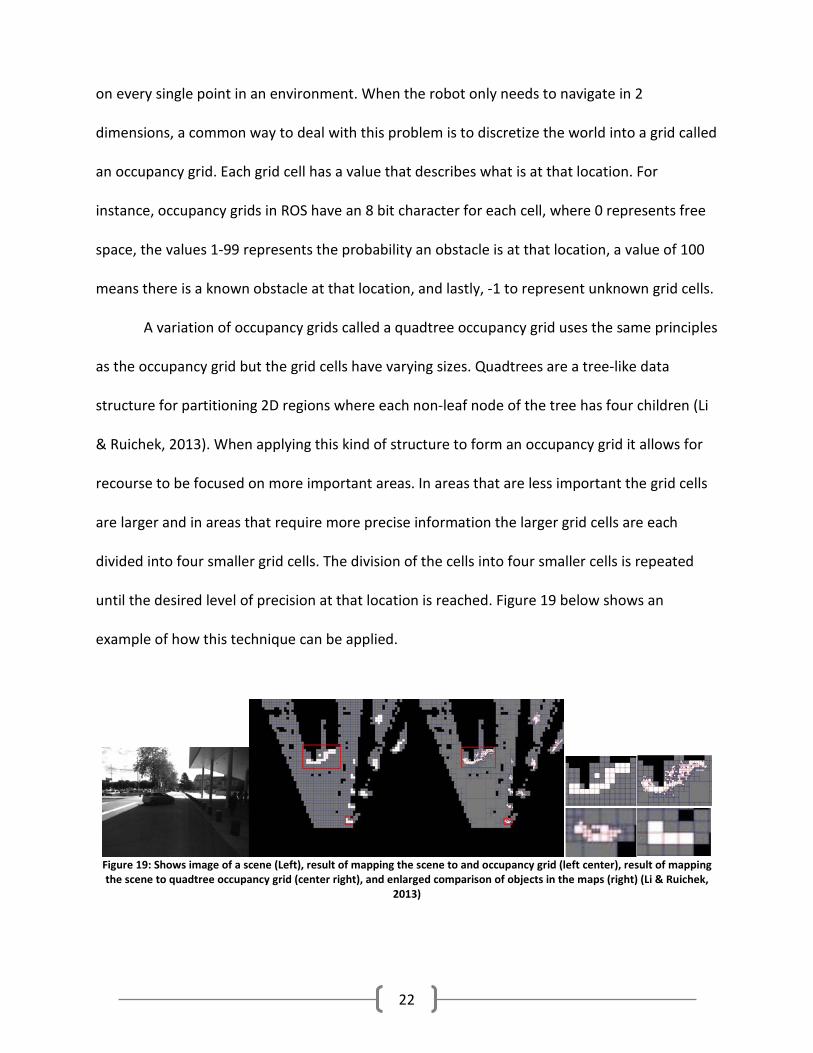
A variation of occupancy grids called a quadtree occupancy grid uses the same principles
as the occupancy grid but the grid cells have varying sizes. Quadtrees are a tree-like data
structure for partitioning 2D regions where each non-leaf node of the tree has four children (Li
& Ruichek, 2013). When applying this kind of structure to form an occupancy grid it allows for
recourse to be focused on more important areas. In areas that are less important the grid cells
are larger and in areas that require more precise information the larger grid cells are each
divided into four smaller grid cells. The division of the cells into four smaller cells is repeated
until the desired level of precision at that location is reached. Figure 19 below shows an
example of how this technique can be applied.
Figure 19: Shows image of a scene (Left), result of mapping the scene to and occupancy grid (left center), result of mapping the scene to quadtree occupancy grid (center right), and enlarged comparison of objects in the maps (right) (Li & Ruichek,
2013)
22

As can be seen in Figure 19, the areas around the obstacles in the quadtree occupancy
grid of the scene have a much higher resolution than the same areas in the normal occupancy
grid. The benefit of this kind of structure is that is saves storage and processing power from
being wasted on areas that don’t need it and can focus those resources where they will be most
effectively used. This also results in a more defined obstacle that can be more precisely
navigated around.
Another application for occupancy grids is to create cost maps. A cost map has the same
grid structure as the occupancy grid but is used to hold different information. The cost map
considers all the information from an occupancy grid map, the physical size of the robot, and
sensor information, such as a laser scanner. The map is used to identify know obstacles and
sensors are used to recognize additional or moved obstacles. The robot’s size to compute the C-
space around the recognized obstacles. The C-space is the area that the center point of the
robot should not navigate through, and gives the grid cells that are part of the C-space a very
high cost. This is a way to ensure that the path planning algorithms don’t pick paths that would
cause collisions with the robot in the physical world. The cost maps use all that information to
compute the cost of moving through each cell in the occupancy grid. This information is then
used by the path planning algorithms that try to find the robot a path from start to finish that
has the lowest cost.
3.7 Mobile Navigation Mobile navigation falls into three main categories: navigation in an unknown, semi-
known and known map. The degree of difficulty of the problem increases the less that is known
about the map. This is because a robot uses the map for localization. In an unknown map the
23

robot is localizing itself to unknown landmarks. In a known and semi- known environment the
robot can predetermine landmarks before it starts to move, however in a semi-known
environment there are obstacles that could have moved, such as a chair or a person. Ideally a
semi-know map has no moved or moving obstacles to plan for the optimal path.
For an unknown environment, the problem has been coined SLAM (Riisgaard & Blas,
2003). SLAM is the process by which a mobile robot can build a map of the environment and at
the same time use this map to compute its location. In SLAM, an autonomous vehicle must
build a map without prior knowledge or update a map. It must then use this map to localize
itself within the environment. One approach to the SLAM problem can be seen below.
Figure 20: Simple approach to the SLAM problem (Riisgaard & Blas, 2003)
As Figure 20 shows, the five main aspects of a SLAM system are: Sensor Data, in this
case a laser scan, landmark extraction algorithm, data association, an Extended Kalman Filter
(EKF), and odometry data. The laser scanner is used to find out obstacles in the map and
24

determine landmarks which can be used. These landmarks are then used to estimate pose by
applying an extended Kalman filter on the location based on the landmarks and the location
based on the odometry.
One approach which is being research is the use of a topological map for localization in a
semi-known environment. In Brazil a group is working to use the Kinect and a topological map
to conduct autonomous surveillance using a mobile robot, while another group, in the United
States, is using the same topological map concept for indoor waypoint navigation (Correa et al.,
2012). In both cases the Kinect is used to gather data about the indoor environment that it is
going to be navigating. This data is used to acquire information about the hallway lengths and
the types of intersections in the hallways, to build a topological map. The intersections are
classified according to Figure 21 below.
Figure 21: Corridor classification for a topological map (Correa et al., 2012)
When generating the map a Progressive Baysian Classifier was used, by the US group,
for corridor classification. This method allowed the robot to take multiple measurements as it
traveled through a corridor to get different angles and distances and then classify the
intersection type. The intersections were used as nodes while the hallways used as edges. A
sample map can be seen in Figure 22 below.
25

Figure 22: An example topological map (Correa et al., 2012)
The edges were associated with a cost, the length of the hallway, to allow for the
shortest path to be calculated, and a heuristic algorithm to be used. This map was then used to
navigate based on right, left and straight directions, which were determined to get to the
waypoint.
In both cases, their testing was successful. One of the benefits of this approach is that it
requires only a low cost sensor to function. This sensor can be used for obstacle avoidance as
well as building the topological map. There was no information for how well this approached
worked if the hallway ahead was filled with people. In a dynamic map, this approach might not
be the best approach. However, a topological map does not need the most accurate
localization, and therefore might lose out to more classical approaches such as an occupancy
grid method.
Research has been done to improve the time it takes to calculate a path and recalculate
a path given a new obstacle in a partially known environment. This is important in partially
known environments where obstacles can move positions and people could be present. The
following approach is used on an occupancy grid with the currently known obstacles.
26

In a partially unknown environment, when an obstacle is detected, the cost of a
particular branch of the path could change and therefore the whole path could change. In
partially known environment or dynamically changing environments a simple map can be used
for features that cannot move, like walls and door, but what happens when a person is in the
way of the path planned. This was addressed, and a D* algorithm was proposed. “The D*
algorithm (Dynamic A*) plans optimal traverses in real-time by incrementally repairing paths to
the robot’s state as new information is discovered” (Stentz, 1995). According to the paper, D*
was very effective when compared against a different re-planning algorithm. Another variation
of the D* algorithm is the focused D*. The focused D* acts to focus the repairs during re-
planning and allows for changing costs during the traversals of the initial path.
Table 2: Results from the execution of four different algorithms (Stentz, 1995)
The table above is for 104, 105, and 106 states. As seen above the D* and focused D*
method both provide significant decreases in time to calculate the path planning. “The off-line
time is the CPU time required to compute the initial path from the goal to the robot” while “the
27

on-line time is the total CPU time for all re-planning operations needed to move the robot from
the start to the goal” (Stentz, 1994). The off-Line time can theoretically be completed before
the robot starts to move, making the full initialization the better algorithm. For a given map the
Focused D* map can be seen in Figure 23 below.
Figure 23: Focused D* map (Stentz, 1995)
Figure 23 above demonstrates that the algorithm will not search the entire map to find
a solution even when recalculating is done, when an obstacle is found. This approach is
beneficial because it will allow for closer to real time calculation of the new route.
Another algorithm is Dijkstra’s algorithm, which finds the shortest path, from a source
node to a destination node, in a graph. It produces a spanning tree which provides the shortest
28

path from a single node to all other nodes in the graph. This algorithm therefore solves the
single source shortest path problem. This algorithm goes through each node and searches the
vertices. It keeps track of visited and unvisited nodes. As edges are explored nodes are added to
the list in increasing distance order from the source. The next process, after an edge is
explored, is to relax the remaining nodes in the tree such that the new lowest cost to them is
updated. This algorithm also expects the edges to all have non-negative weights. This can be
used to search occupancy grids in robotics because the graph can be considered four (up,
down, left, and right) or eight (up, down, left, right, four diagonals) way connected. It is a fairly
simple algorithm that is used for its ease, although re-planning is not as fast as the previously
mentioned algorithms the ease in which Dijkstra’s algorithm can be programmed are beneficial
for preliminary tests. In a relatively known environment Dijkstra’s algorithm performs well due
to the limited number of recalculations that need to be made.
Each algorithm has its benefits and downfalls. Some perform better in real time,
however, are more complicated algorithms; others are faster at the initial calculation of a path
than re-planning a path. Either way the algorithm used would be task dependent and
determined by the state of the map: known, semi-known and unknown.
3.8 GUI Design Our goal is to have a robot that can be interacted with, either directly via a touchscreen
or remotely via a laptop. This will require some sort of interface between the robot controls
and the user. In designing and implementing a useful product, it is important that a user
interface be well designed so that the user can easily and successfully use the product.
29

Much of the research on graphical user interfaces (GUI) is the same. There is a focus on
generating usable, adaptable designs that are simple in layout but offer many features. Data
structures must be dynamic and communication protocols must be unified. There was a focus
on creating design patterns to use as a template for most layout and design of the GUI
(Luostarinen, Manner, Maatta, & Jarvinen, 2010).
One example of such software architecture for GUI’s is the Model/View/Controller
pattern as seen in Figure 24. The model is where the data is stored and most of the
computation is handled. The view is what displays the GUI and the data in it. Each view has its
own controller to handle user input and communicate with the model as necessary. The
communication between model, view, and controller has an established format using the
interfaces defined.
Figure 24: Shows the architecture for a Model/View/Controller pattern.
30
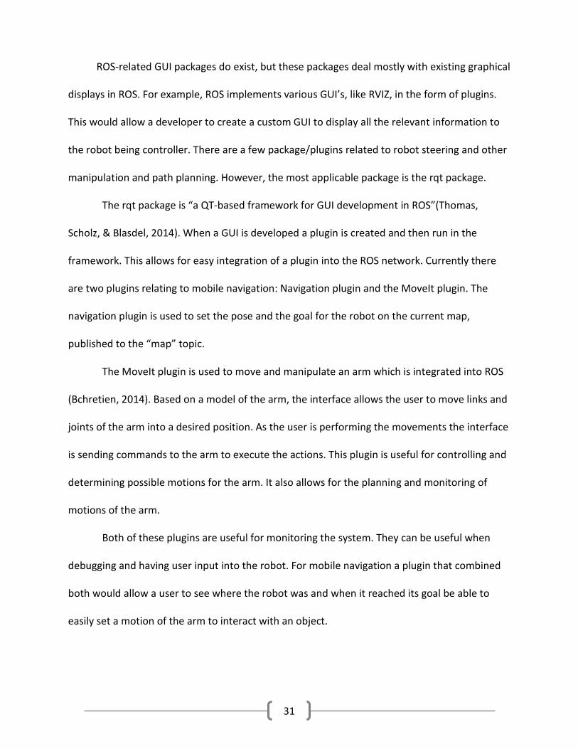
ROS-related GUI packages do exist, but these packages deal mostly with existing graphical
displays in ROS. For example, ROS implements various GUI’s, like RVIZ, in the form of plugins.
This would allow a developer to create a custom GUI to display all the relevant information to
the robot being controller. There are a few package/plugins related to robot steering and other
manipulation and path planning. However, the most applicable package is the rqt package.
The rqt package is “a QT-based framework for GUI development in ROS”(Thomas,
Scholz, & Blasdel, 2014). When a GUI is developed a plugin is created and then run in the
framework. This allows for easy integration of a plugin into the ROS network. Currently there
are two plugins relating to mobile navigation: Navigation plugin and the MoveIt plugin. The
navigation plugin is used to set the pose and the goal for the robot on the current map,
published to the “map” topic.
The MoveIt plugin is used to move and manipulate an arm which is integrated into ROS
(Bchretien, 2014). Based on a model of the arm, the interface allows the user to move links and
joints of the arm into a desired position. As the user is performing the movements the interface
is sending commands to the arm to execute the actions. This plugin is useful for controlling and
determining possible motions for the arm. It also allows for the planning and monitoring of
motions of the arm.
Both of these plugins are useful for monitoring the system. They can be useful when
debugging and having user input into the robot. For mobile navigation a plugin that combined
both would allow a user to see where the robot was and when it reached its goal be able to
easily set a motion of the arm to interact with an object.
31

3.9 Object Recognition One way to perform object recognition is to perform image matching. This method
works well when the object is always in the same orientation based on the viewing angle.
To perform image recognition or image matching the OpenCV library for python could
be used. It provides existing methods, such as MatchTemplate(), which compares an image
patch to an image. There are multiple algorithms which that method could use that could be
used for matching and we considered each one for our purposes. The image patch is a small
image, as big as or smaller than the image. The images are compared by sweeping the image
patch through the image, using various functions for comparison, to try and find a match. The
various function types are:
• Square difference matching method (Equation 1 and Equation 4)
• Correlation matching method (Equation 2 and Equation 5)
• Correlation Coefficient matching methods (Equation 3 and Equation 6)
These are the three main methods, there are also normalized methods for each of the three
methods mentioned above. The formula for each method can be seen below:
Equation 1: Square Difference method
Equation 2: Correlation matching method
32

Equation 3: Correlation Coefficient method
The formula for the normalized versions can be seen below:
Equation 4: Square Difference method normalized
Equation 5: Correlation matching method normalized
Equation 6: Correlation Coefficient method normalized
The difference between each of the methods is their accuracy for matches. The square
difference methods are the least accurate, then the correlation matching methods and finally
the correlation coefficient methods are the most accurate. However, with higher accuracy
comes a higher computation cost. Therefore, a balance must be found between accuracy and
computations.
33

4.0 Methodology From our research, we can begin to put together a solution to reach our goal. This
involved disassembling the platform and understanding its current state while also exploring
the possible upgrades; for example, software architecture, electrical schematics and
manipulator designs.
4.1 Robot Design Overview The robot started off with a GPS module, an IMU module, stereo vision and a 360
degree ultrasonic scan. A visual overview can be seen in Figure 25.
Figure 25: Original robot overview (LeBlanc, Patel, & Rashid, 2012)
34

To satisfy our goals the robot needed to have the electronics reorganized and the
platform updated. This meant that the robot needed to be taken apart and sent back to
Segway. The robot before it was taken apart can be seen in Figure 26 and Figure 27.
Figure 26: Picture of the Rear of the robot at the beginning of the MQP
Figure 27: Picture of the front of the Robot at beginning of MQP
35

Once the robot was taken apart the Segway platform, was returned. The returned
platform and control box, seen in red can be seen in Figure 28.
Figure 28: Segway control box before servicing
As seen in Figure 28 and Figure 29, the control box, circled in red, was upgraded and an
additional auxiliary battery was mounted to provide external power to electronics, as seen in
Figure 29.
Figure 29: Segway Control box after servicing
Evaluation of the electrical schematic was completed while the Segway platform was
getting upgraded. The original electrical schematic can be seen in Figure 30.
36

Figure 30: Original Electrical Schematic (LeBlanc, Patel, & Rashid, 2012)
Since our application for the robot was to navigate indoors, while the previous robot
was designed for outdoor use outdoors, a few of the electronics were not needed. This
included the GPS, the powered USB hub and the E-Stop circuits. A revised electrical schematic
was developed and electronics for the arm was added. This preliminary schematic can be seen
in Figure 31.
Figure 31: Proposed electrical schematic update
37

Looking at the current robot it was apparent that the current power distribution board
was not appropriate for a professional looking robot. It also had no room to include the power
and controls for the newly designed arm. Although functional, visually it was unprofessional
and there were exposed connections for the wires. The original power distribution can be seen
in Figure 32 below. Therefore, it was decided that a new PCB would be designed to allow for
the current power distribution schematic as well as future expansion upon the platform.
Figure 32: Original Power distribution board
Finally to set up the robot, the touchscreen computer and the desktop was upgraded to
Ubuntu 12.04 and ROS Hydro. This meant that all the previous ROS packages had to be updated
to work in a catkin workspace.
38

4.2 Arm Design The design process for the arm began with the fourteen arm design parameters
discussed earlier in Section 3.2 Arm Design. As is typical with design projects, there is always at
least one parameter that is defined for you, and in this project that was the working envelope,
which is the region of space the arm can occupy. For us, this was defined by the top plate of the
Segway RMP. Based on this constraint, along with the design goals for the arm, which are
enumerated below, the desired working space of the arm was defined. From there, the
iterative method was used to define the remaining parameters.
Arm design goals:
• 5lb max object weight, the approximate weight of a full 32oz Nalgene water bottle
• Maximum object size of 5in diameter, slightly larger than the diameter of a 32oz
Nalgene water bottle
• Retrieve obj. from height of 30 - 60in (30in above robot top), the typical height of a desk
or countertop
• Be able to hit a square 1 inch target, the size of an elevator button
• 2 foot extension from front of robot, the typical depth of a counter or desk
Each design iteration was assessed based on its perceived ability to complete each of
these goals, and the effort it would take to ensure the goals were achieved. While not
completely quantitative, this analysis made the design decisions more objective and less about
personal preferences.
39

4.2.1 Arm Concept 1 - Rack & Pinion
This design was based on the linear motion of a “sled” for the arm to be mounted on
using dual rack and pinions, making the reach of the arm uniform throughout the vertical range.
Compared to the linkage design, however, this design is complicated, requires two motors to
run in unison, and may be difficult to make not backdrivable. Because of the complexity of the
design, this concept would likely be more expensive to implement.
Figure 33: Arm concept 2 - rack & pinion design (Corperation, 2012)
4.2.2 Arm Concept 2 - Lead Screw
This design was also based on the linear motion of a sled for the arm to be mounted on,
but in a more simplified fashion using a lead screw. This design would produce the same linear
motion of a sled as the rack and pinion, while being much less complicated. Lead screws are an
extremely efficient method of turning (pun intended) rotational motion into linear motion, but
when the efficiency of a lead screw exceeds 50%, the lead screw becomes back-drivable. This
would be undesirable for our application.
40

Figure 34: Arm concept 3 - lead screw design (Lipsett, 2013)
4.2.3 Arm Concept 3 - Linkage
This concept was designed with simplicity in mind. Using parallel four bar linkages with
the 3-link arm mounted to the joint coupler, we were able to synthesize an arm design with a
workspace that encompassed all of the required design goals. The benefits of this design
include its simplicity, the ease of measuring the linkage position and making the linkage not
backdrivable, and lower cost.
Figure 35: Arm concept 1 – linkage design (Corperation, 2012)
41

The downside of this design is due to the non-linear coupler curve. Because of this, the
horizontal range of the gripper is a function of the linkage position. Although not a mechanical
issue, this could pose a problem in the arm control. After reviewing the pros and cons of each
arm concept, we determined that the best option was to move forward with the linkage design
option.
4.2.4 Linkage Design Iterations
Once we decided on the linkage design as a basis for the final arm design, we went
through several further design iterations. The goals of these further design modifications were
to improve upon the functionality of the arm assembly, while simplifying the design as much as
possible and cutting down on material and component costs. Motor selection was likely the
most crucial aspect of this process, as the motors and their gearing would determine the
maximum capabilities of the arm.
All designing and prototyping was done using SolidWorks, which allowed us to go
through numerous iterations without wasting our money buying prototyping parts that
wouldn’t end up in the final design. The downside of this design paradigm was that without
being able to physically build and test design concepts, it was up to the discretion of the group
to analyze the 3D models of the designs and determine their feasibility and best functionality.
The design of the arm was split into 3 major sections: the tower and linkage, the arm,
and the wrist and gripper. Being the base for the rest of the design, we first decided to tackle
the tower and linkage design. It was determined that in order to achieve the necessary torque
to lift the arm and ensure the system was not backdrivable, while still staying within budget, a
42

significant gearing ratio would be required on the motor lifting the linkage. Motor selection for
the main linkage motor was a process, as we had to take a number of variables into account,
including operating voltage, current draw, stall torque, no load speed, and of course price.
Using all of these criteria, we eventually narrowed the choices down to one, a CIM motor,
which is commonly used in FIRST Robotics. With this motor, we calculated a desired minimum
gearing ratio of 1:25 in order to ramp up the output torque of the motor.
To construct the tower on which the motor and linkage would be mounted, we wanted
to keep it as modular and simple as possible, so we decided to construct it out of 80/20®
extruded aluminum. In order to keep as low a profile as possible, it was decided to mount the
motor vertically inside the tower and use a bevel gear and pinion set to transfer the rotational
motion 90 degrees to the horizontal. While effective, this design proved to add unnecessary
costs and complexity to the linkage design, and was ultimately scrapped for a horizontally
mounted motor design with no bevel gears. This enabled us to remove two gears for the
gearbox and actually allowed for a larger gearbox footprint, giving us more room to work with.
With the bevel gear design, a gearing ratio of 1:~51 was achieved, but in the final design, with
the bevel gears removed, an even greater ratio of 1:~56 was achieved. The gear and motor
mounts were machined from 0.25” thick aluminum plate and mounted directly to the sides of
the tower. For the material of the links, extruded aluminum offered the best strength/weight
ratio. Using SolidWorks SimulationXpress Analysis Wizard, Finite Element Analysis (FEA) was
performed to ensure that the designed aluminum parts would be able to meet the design
specifications. An example of this analysis can be seen in Figure 36, and the remaining results
can be seen in Appendix A.
43

Figure 36: Stress diagram from SolidWorks FEA
Figure 37: Completed SolidWorks arm design (Corperation, 2012)
44

The results of this analysis showed minimal deflection in the range of 0 to .4 millimeters,
allowing the design to be finalized. The final design in SolidWorks is shown in Figure 37. Due to
time and budgetary constraints, the remaining arm components were obtained from stock in
the WPI labs. For the power of the arm and wrist links and the gripper, suitable motors, belts,
pulleys, and gears were selected from the stock available to us in our lab. Analog
potentiometers were obtained from the ECE lab.
4.2.5 Linkage Analysis
The four bar linkage serves as a method to adjust the height of the two link arm, which
is mounted to the coupler of the linkage as shown in Figure 38 below. The “0” coordinate frame
of the two link arm, shown in Figure 39, corresponds to the “c” coordinate frame as seen in
Figure 38. While adjusting the height of the coupler, cy, a horizontal offset cx along the xb axis is
also adjusted. These two offsets are directly influenced by the angle θ of the linkage as
described by the equations below.
45

Figure 38: Linkage diagram
Dimension Equations:
𝑎𝑎1 = 𝑎𝑎2
𝑏𝑏1 = 𝑏𝑏2
Position Equations:
𝑐𝑐𝑦𝑦 = 𝑐𝑐 ∗ 𝑠𝑠𝑠𝑠𝑠𝑠 (𝜃𝜃)
𝑐𝑐𝑥𝑥 = 𝑐𝑐 ∗ 𝑐𝑐𝑐𝑐𝑠𝑠(𝜃𝜃)
Angle Equations:
𝜃𝜃 = 𝑠𝑠𝑠𝑠𝑠𝑠−1 �𝑐𝑐𝑦𝑦𝑐𝑐� = 𝑐𝑐𝑐𝑐𝑠𝑠−1(
𝑐𝑐𝑥𝑥𝑐𝑐
)
46

4.2.6 Arm Analysis and Forward Kinematics
The following figures, tables, and equations illustrate the kinematics of the arm and
linkage mechanism. Figure 39 below shows the Denavit-Hartenberg reference frames on a
rendered SolidWorks image, starting with the base frame, B, and ending at T, the tool frame.
The transformations between these frames are described in Table 3 and the equations below.
The forward kinematics of the mechanism describes the position of the tool frame based on the
joint angles of the system.
Figure 39: Kinematic diagram
47

Denavit–Hartenberg Table:
Frame # 𝜃𝜃 𝑑𝑑 𝑎𝑎 α
1 𝜃𝜃*B 0 a1 0
2 𝜃𝜃1 = -𝜃𝜃B d2 a2 90
3 𝜃𝜃*2 0 a3 0
T 𝜃𝜃*3 0 aT 0
Table 3: Denavit–Hartenberg Table
Transformation matrix from Frame B to Frame 1:
𝑇𝑇𝐵𝐵1 = 𝐴𝐴𝐵𝐵1 = 𝑅𝑅𝑐𝑐𝑅𝑅(𝑧𝑧,𝜃𝜃𝐵𝐵)𝑇𝑇𝑇𝑇𝑎𝑎𝑠𝑠𝑠𝑠(0, 0, 𝑑𝑑1)𝑇𝑇𝑇𝑇𝑎𝑎𝑠𝑠𝑠𝑠(𝑎𝑎1, 0, 0)𝑅𝑅𝑐𝑐𝑅𝑅(𝑥𝑥,𝛼𝛼1)
= �
𝑐𝑐𝜃𝜃𝐵𝐵 −𝑠𝑠𝜃𝜃𝐵𝐵𝑐𝑐𝛼𝛼1 𝑠𝑠𝜃𝜃𝐵𝐵𝑠𝑠𝛼𝛼1
𝑎𝑎1𝑐𝑐𝜃𝜃𝐵𝐵 𝑠𝑠𝜃𝜃𝐵𝐵 𝑐𝑐𝜃𝜃𝐵𝐵𝑐𝑐𝛼𝛼1
−𝑐𝑐𝜃𝜃𝐵𝐵𝑠𝑠𝛼𝛼1𝑎𝑎1𝑠𝑠𝜃𝜃𝐵𝐵
0 𝑠𝑠𝛼𝛼1 𝑐𝑐𝛼𝛼1 𝑑𝑑1 0 0 0 1
� = �
𝑐𝑐𝜃𝜃𝐵𝐵 −𝑠𝑠𝜃𝜃𝐵𝐵 0 𝑎𝑎1𝑐𝑐𝜃𝜃𝐵𝐵 𝑠𝑠𝜃𝜃𝐵𝐵 𝑐𝑐𝜃𝜃𝐵𝐵 0 𝑎𝑎1𝑠𝑠𝜃𝜃𝐵𝐵
0 0 1 0 0 0 0 1
�
Transformation matrix from Frame 1 to Frame 2:
𝑇𝑇12 = 𝐴𝐴12 = 𝑅𝑅𝑐𝑐𝑅𝑅(𝑧𝑧, 𝜃𝜃1)𝑇𝑇𝑇𝑇𝑎𝑎𝑠𝑠𝑠𝑠(0, 0,𝑑𝑑2)𝑇𝑇𝑇𝑇𝑎𝑎𝑠𝑠𝑠𝑠(𝑎𝑎2, 0, 0)𝑅𝑅𝑐𝑐𝑅𝑅(𝑥𝑥,𝛼𝛼2)
= �
𝑐𝑐𝜃𝜃1 −𝑠𝑠𝜃𝜃1𝑐𝑐𝛼𝛼2 𝑠𝑠𝜃𝜃1𝑠𝑠𝛼𝛼2
𝑎𝑎2𝑐𝑐𝜃𝜃1 𝑠𝑠𝜃𝜃1 𝑐𝑐𝜃𝜃1𝑐𝑐𝛼𝛼2
−𝑐𝑐𝜃𝜃1𝑠𝑠𝛼𝛼2𝑎𝑎2𝑠𝑠𝜃𝜃1
0 𝑠𝑠𝛼𝛼2 𝑐𝑐𝛼𝛼2 𝑑𝑑2 0 0 0 1
�
Transformation matrix from Frame 2 to Frame 3:
𝑇𝑇23 = 𝐴𝐴23 = 𝑅𝑅𝑐𝑐𝑅𝑅(𝑧𝑧,𝜃𝜃2)𝑇𝑇𝑇𝑇𝑎𝑎𝑠𝑠𝑠𝑠(0, 0,𝑑𝑑3)𝑇𝑇𝑇𝑇𝑎𝑎𝑠𝑠𝑠𝑠(𝑎𝑎3, 0, 0)𝑅𝑅𝑐𝑐𝑅𝑅(𝑥𝑥,𝛼𝛼3)
= �
𝑐𝑐𝜃𝜃2 −𝑠𝑠𝜃𝜃2𝑐𝑐𝛼𝛼1 𝑠𝑠𝜃𝜃2𝑠𝑠𝛼𝛼1
𝑎𝑎3𝑐𝑐𝜃𝜃2 𝑠𝑠𝜃𝜃2 𝑐𝑐𝜃𝜃2𝑐𝑐𝛼𝛼1
−𝑐𝑐𝜃𝜃2𝑠𝑠𝛼𝛼1𝑎𝑎3𝑠𝑠𝜃𝜃2
0 𝑠𝑠𝛼𝛼1 𝑐𝑐𝛼𝛼1 𝑑𝑑1 0 0 0 1
� = �
𝑐𝑐𝜃𝜃2 −𝑠𝑠𝜃𝜃2 0 𝑎𝑎3𝑐𝑐𝜃𝜃2 𝑠𝑠𝜃𝜃2 𝑐𝑐𝜃𝜃2 0 𝑎𝑎3𝑠𝑠𝜃𝜃2 0 0 1 0 0 0 0 1
�
48

Transformation matrix from Frame 3 to Frame T:
𝑇𝑇3𝑇𝑇 = 𝐴𝐴3𝑇𝑇 = 𝑅𝑅𝑐𝑐𝑅𝑅(𝑧𝑧,𝜃𝜃3)𝑇𝑇𝑇𝑇𝑎𝑎𝑠𝑠𝑠𝑠(0, 0,𝑑𝑑𝑇𝑇)𝑇𝑇𝑇𝑇𝑎𝑎𝑠𝑠𝑠𝑠(𝑎𝑎𝑇𝑇 , 0, 0)𝑅𝑅𝑐𝑐𝑅𝑅(𝑥𝑥,𝛼𝛼𝑇𝑇)
= �
𝑐𝑐𝜃𝜃3 −𝑠𝑠𝜃𝜃3𝑐𝑐𝛼𝛼𝑇𝑇 𝑠𝑠𝜃𝜃3𝑠𝑠𝛼𝛼𝑇𝑇
𝑎𝑎𝑇𝑇𝑐𝑐𝜃𝜃3 𝑠𝑠𝜃𝜃3 𝑐𝑐𝜃𝜃3𝑐𝑐𝛼𝛼𝑇𝑇
−𝑐𝑐𝜃𝜃3𝑠𝑠𝛼𝛼𝑇𝑇𝑎𝑎𝑇𝑇𝑠𝑠𝜃𝜃3
0 𝑠𝑠𝛼𝛼𝑇𝑇 𝑐𝑐𝛼𝛼𝑇𝑇 𝑑𝑑𝑇𝑇 0 0 0 1
� = �
𝑐𝑐𝜃𝜃3 −𝑠𝑠𝜃𝜃3 0 𝑎𝑎𝑇𝑇𝑐𝑐𝜃𝜃3 𝑠𝑠𝜃𝜃3 𝑐𝑐𝜃𝜃3 0 𝑎𝑎𝑇𝑇𝑠𝑠𝜃𝜃3 0 0 1 0 0 0 0 1
�
Transformation matrix from Frame B to Frame T:
𝑇𝑇𝐵𝐵𝑇𝑇 = 𝐴𝐴𝐵𝐵1𝐴𝐴12𝐴𝐴23𝐴𝐴3𝑇𝑇
= �
𝑐𝑐𝜃𝜃𝐵𝐵 −𝑠𝑠𝜃𝜃𝐵𝐵 0 𝑎𝑎1𝑐𝑐𝜃𝜃𝐵𝐵 𝑠𝑠𝜃𝜃𝐵𝐵 𝑐𝑐𝜃𝜃𝐵𝐵 0 𝑎𝑎1𝑠𝑠𝜃𝜃𝐵𝐵
0 0 1 0 0 0 0 1
��
𝑐𝑐𝜃𝜃1 −𝑠𝑠𝜃𝜃1𝑐𝑐𝛼𝛼2 𝑠𝑠𝜃𝜃1𝑠𝑠𝛼𝛼2
𝑎𝑎2𝑐𝑐𝜃𝜃1 𝑠𝑠𝜃𝜃1 𝑐𝑐𝜃𝜃1𝑐𝑐𝛼𝛼2
−𝑐𝑐𝜃𝜃1𝑠𝑠𝛼𝛼2𝑎𝑎2𝑠𝑠𝜃𝜃1
0 𝑠𝑠𝛼𝛼2 𝑐𝑐𝛼𝛼2 𝑑𝑑2 0 0 0 1
��
𝑐𝑐𝜃𝜃2 −𝑠𝑠𝜃𝜃2 0 𝑎𝑎3𝑐𝑐𝜃𝜃2 𝑠𝑠𝜃𝜃2 𝑐𝑐𝜃𝜃2 0 𝑎𝑎3𝑠𝑠𝜃𝜃2 0 0 1 0 0 0 0 1
��
𝑐𝑐𝜃𝜃3 −𝑠𝑠𝜃𝜃3 0 𝑎𝑎𝑇𝑇𝑐𝑐𝜃𝜃3 𝑠𝑠𝜃𝜃3 𝑐𝑐𝜃𝜃3 0 𝑎𝑎𝑇𝑇𝑠𝑠𝜃𝜃3 0 0 1 0 0 0 0 1
�
4.2.7 Inverse Kinematics
The inverse kinematics of a robotic arm describe the joint angles based on the desired
position of the end of arm tooling (EoAT). There can be multiple solutions to the inverse
kinematic equations, and each solution will correspond to a different configuration of the arm
which places the tool frame in the desired position.
Position vectors of (EoAT):
�𝑝𝑝𝑥𝑥𝑝𝑝𝑦𝑦𝑝𝑝𝑧𝑧� = �
𝑎𝑎1 cos(𝜃𝜃𝐵𝐵) + 𝑎𝑎𝑇𝑇cos (𝜃𝜃2 + 𝜃𝜃3) + 𝑎𝑎3cos (𝜃𝜃2)𝑎𝑎1 sin(𝜃𝜃𝐵𝐵)
𝑎𝑎𝑇𝑇sin(𝜃𝜃2 + 𝜃𝜃3) + 𝑎𝑎3sin (𝜃𝜃2)�
Inverse kinematics equations:
𝜽𝜽𝑩𝑩 = 𝐬𝐬𝐬𝐬𝐬𝐬−𝟏𝟏 �𝒑𝒑𝒚𝒚𝒂𝒂𝟏𝟏�
49

�𝑝𝑝𝑥𝑥 − 𝑎𝑎1�1 − �𝑝𝑝𝑦𝑦𝑎𝑎1�2�
2
= (𝑎𝑎𝑇𝑇cos (𝜃𝜃2 + 𝜃𝜃3) + 𝑎𝑎3cos (𝜃𝜃2))2
𝑝𝑝𝑥𝑥2 − 2𝑝𝑝𝑥𝑥𝑎𝑎1�1 − �𝑝𝑝𝑦𝑦𝑎𝑎1�2
+ 𝑎𝑎12 �1 − �𝑝𝑝𝑦𝑦𝑎𝑎1�2�
= 𝑎𝑎𝑇𝑇2𝑐𝑐𝑐𝑐𝑠𝑠2(𝜃𝜃2 + 𝜃𝜃3) + 𝑎𝑎32𝑐𝑐𝑐𝑐𝑠𝑠2(𝜃𝜃2) + 2𝑎𝑎𝑇𝑇𝑎𝑎3 cos(𝜃𝜃2 + 𝜃𝜃3) cos(𝜃𝜃2)
𝑝𝑝𝑧𝑧2 = 𝑎𝑎𝑇𝑇2𝑠𝑠𝑠𝑠𝑠𝑠2(𝜃𝜃2 + 𝜃𝜃3) + 𝑎𝑎32𝑠𝑠𝑠𝑠𝑠𝑠2(𝜃𝜃2) + 2𝑎𝑎𝑇𝑇𝑎𝑎3 sin(𝜃𝜃2 + 𝜃𝜃3) sin(𝜃𝜃2)
𝑝𝑝𝑥𝑥2 + 𝑝𝑝𝑧𝑧2 − 2𝑝𝑝𝑥𝑥𝑎𝑎1�1 − �𝑝𝑝𝑦𝑦𝑎𝑎1�2
+ 𝑎𝑎12 �1 − �𝑝𝑝𝑦𝑦𝑎𝑎1�2�
= 𝑎𝑎𝑇𝑇2�𝑐𝑐𝑐𝑐𝑠𝑠2(𝜃𝜃2 + 𝜃𝜃3) + 𝑠𝑠𝑠𝑠𝑠𝑠2(𝜃𝜃2 + 𝜃𝜃3)� + 𝑎𝑎32�𝑐𝑐𝑐𝑐𝑠𝑠2(𝜃𝜃2) + 𝑠𝑠𝑠𝑠𝑠𝑠2(𝜃𝜃2)�
+ 2𝑎𝑎𝑇𝑇𝑎𝑎3(cos(𝜃𝜃2 + 𝜃𝜃3) cos(𝜃𝜃2𝜃𝜃2) + sin(𝜃𝜃2 + 𝜃𝜃3) sin(𝜃𝜃2))
cos(𝜃𝜃3) =
𝑝𝑝𝑥𝑥2 + 𝑝𝑝𝑧𝑧2 − 2𝑝𝑝𝑥𝑥𝑎𝑎1�1 − �𝑝𝑝𝑦𝑦𝑎𝑎1�2
+ 𝑎𝑎12 �1 − �𝑝𝑝𝑦𝑦𝑎𝑎1�2� − 𝑎𝑎𝑇𝑇2 − 𝑎𝑎32
2𝑎𝑎𝑡𝑡𝑎𝑎3
𝜽𝜽𝟑𝟑 = 𝐜𝐜𝐜𝐜𝐬𝐬−𝟏𝟏
⎝
⎜⎜⎛𝒑𝒑𝒙𝒙
𝟐𝟐 + 𝒑𝒑𝒛𝒛𝟐𝟐 − 𝟐𝟐𝒑𝒑𝒙𝒙𝒂𝒂𝟏𝟏�𝟏𝟏 − �𝒑𝒑𝒚𝒚𝒂𝒂𝟏𝟏�𝟐𝟐
+ 𝒂𝒂𝟏𝟏𝟐𝟐 �𝟏𝟏 − �𝒑𝒑𝒚𝒚𝒂𝒂𝟏𝟏�𝟐𝟐� − 𝒂𝒂𝑻𝑻𝟐𝟐 − 𝒂𝒂𝟑𝟑𝟐𝟐
𝟐𝟐𝒂𝒂𝑻𝑻𝒂𝒂𝟑𝟑
⎠
⎟⎟⎞
50

“Elbow down” (A) and “elbow up” (B) solutions to the arm inverse kinematics:
Figure 40: Elbow down (A) and elbow up (B) solutions to the arm inverse kinematics (Computing, 2013)
Solving for θ2:
ϕ = atan2(𝑝𝑝𝑦𝑦,𝑝𝑝𝑥𝑥)
ψ = atan2(𝑎𝑎𝑇𝑇 sin(θ3) ,𝑎𝑎3 + 𝑎𝑎𝑇𝑇cos (θ3))
𝛉𝛉𝟐𝟐 = 𝛟𝛟−𝛙𝛙
4.3 Arm Control Having decided on the arm components, the next step was to integrate the components.
The motors would need motor drivers and a controller to control the motors during operation.
4.3.1 Hardware
There were three different types of motors to operate: one Vex servo motor to operate
the gripper, two Globe motors (P/N: 415A832) to operate the two-link arm, and one CIM motor
(P/N: 217-2000) to operate the linkage mechanism to lift and lower the two-link arm. All of
these can be seen in Figure 41.
51

Figure 41: Manipulator design
Each actuator had different power requirements to operate. All of these motors
operated using pulse-width modulation (PWM) signals. There were a couple options to
consider: design and print a proprietary motor driver board using a chip, or buy a commercially
available driver. Given the lack of expertise in PCB design and motor drivers, as well as the
limited budget, commercially available boards were the cheapest and easiest option.
The CIM motor under a free loading requires about 3A; while at stall, it draws 133A.
Given that the power supply does not put out that much current, a board was necessary to
handle at least what could be output by the supply which was about 25A. A motor driver from
Polulu (VNH2SP30 Motor driver board) was found to be satisfactory to handle the power
supplied from the battery. The performance specifications can be found in Table 4Table 4.
Vex servo motor
Globe motors
CIM motor
52

Table 4: Pololu motor driver performance specifications
The CIM motor specifications can be seen in Table 5. Given the limitations of the power
supply, we would be under supplying the CIM motor. The power would be compensated for in
the gearing.
Table 5: CIM motor performance specifications
The Polulu motor board would be more powerful than necessary for the globe motors. It
also would be more expensive to purchase these drivers since they only power one motor each.
Some further searching found some dual channel drivers from Canakit (L298 dual H-bridge
circuit) that would be sufficient enough for 12V motors, as each channel can handle up to 2A.
The globe motors were scrapped off existing equipment in the lab, but were calculated
to be powerful enough to move the arm links. They only consumed 50mA in a no-load situation.
This would easily be supplied by the Canakit motor drivers.
53

Two microcontrollers were considered to act as the motor controller for the four
motors: Arduino and PIC. Arduino microcontrollers are robust boards with lots of external
community support for development. PIC microcontrollers range in size and ability, and were
most commonly used within the lab. The PIC32 and USB starter kit were investigated from the
PIC family of microcontrollers. There were some considerations in deciding on a
microcontroller. The board needed to suffice in meeting the needs of the hardware while being
expandable for the future. The biggest factor that played into the selection was familiarity and
community support.
Figure 42: Arduino and motor drivers mounted onto the arm assembly
54

An Arduino Mega 2560 was the microcontroller selected, as we were most familiar with
this controller. Arduino has a lot of online support which would make development easier. The
board also had plenty of digital I/O as well as analog inputs and PWM outputs. This would easily
meet the needs of the arm, without being overly complex. All of the hardware was mounted to
the back of the arm assembly on an acrylic plate as seen in Figure 42.
Two wire harnesses were made for the motor drivers to connect the control pins to the
Arduino. The pin layouts can be seen in Table 6, Table 7, and Table 8.
Table 6: Vex servo pin layout Table 7: Canakit motor driver control
pin layout Table 8: Pololu motor driver control pin
layout
As can be seen in Figure 42, the harnesses ran from the motor drivers to the Arduino.
Some of the Arduino pins were expanded onto the breadboard in order to supply the 5V power
to sensors. The GNDs had to be unified to keep all reference sources on the same signal.
4.3.2 Communication
Moving forward with the design, in order to properly operate the arm, a communication
protocol had to be developed to communicate between the microcontroller and the computer.
The main computer would communicate joint positions to the microcontroller over serial USB
in order to move the arm to a desired position. The communication structure was the same for
55

sending and receiving, simplifying some of the code. The start byte, the carriage return
character, was sent to signal the PC or microcontroller to start to read the data in. An ending
byte, a newline character, would signify the end of the data transfer. Figure 43 breaks down the
total byte structure of the command and feedback sent to and from the Arduino.
Figure 43: Byte structure for communication to and from the Arduino
The reason that the joints were sent in four bytes was so that the converted analog
signal could be sent instead of the actual angles. Since there are 1024 values in a 10 bit ADC,
four bytes were needed for data transfer. This allowed for more accurate angles to be
calculated on the computer and fully transferred to the Arduino without truncation or
rounding. Each byte sent was the bit structure for an ASCII character. The Arduino and Python
serial libraries supported byte-wise transmission, which was easier to use than bit-wise
transmission. In order to maintain synconized communication, the Arduino would only send
data when the computer sent a command. In addition, angles out of range would be sent to
query information.
The only data to send back to the main computer would be the actual joint positions.
This would allow us to monitor the movements of joints. Other actuation data could be
configured to send as well but we felt it would slow down the communication and potentially
limit the ability of the arm.
56

4.3.3 Control
For autonomous control or teleoperation of the arm, a control system must be
implemented to properly articulate the arm. For controlling the movements of the arm, a
Proportional, Integral, Derivative (PID) control structure was used. Time and experience were a
contributing factor at this point in the design. It made more sense to use a control structure
that was familiar than attempt to develop a new one or implement a previously unknown
structure.
PID control uses desired positions and actual positions to calculate an error, a rate of
change and a steady-state error buildup. The summation of these three factors results in a
motor output to correct the error in the system. The weighting of each component can be
tuned to produce a smooth and accurate control system for a manipulator or any other
application. A basic PID control flow can be seen in Figure 44.
SETPOINT
I
P
D
MOTOR
POTENTIOMETER
Σ+
+
+Σ+
-
Figure 44: Basic PID control flow
Proper operation requires each link to be coordinated together. Therefore, each joint
needed a control structure to move into place. During execution of the control loop, the actual
position values are read and the set-points of the system are updated as necessary from the
57
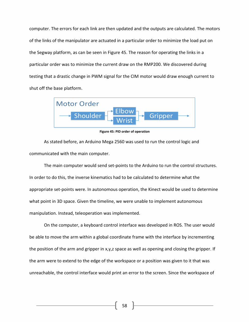
computer. The errors for each link are then updated and the outputs are calculated. The motors
of the links of the manipulator are actuated in a particular order to minimize the load put on
the Segway platform, as can be seen in Figure 45. The reason for operating the links in a
particular order was to minimize the current draw on the RMP200. We discovered during
testing that a drastic change in PWM signal for the CIM motor would draw enough current to
shut off the base platform.
ShoulderElbowWrist
Gripper
Figure 45: PID order of operation
As stated before, an Arduino Mega 2560 was used to run the control logic and
communicated with the main computer.
The main computer would send set-points to the Arduino to run the control structures.
In order to do this, the inverse kinematics had to be calculated to determine what the
appropriate set-points were. In autonomous operation, the Kinect would be used to determine
what point in 3D space. Given the timeline, we were unable to implement autonomous
manipulation. Instead, teleoperation was implemented.
On the computer, a keyboard control interface was developed in ROS. The user would
be able to move the arm within a global coordinate frame with the interface by incrementing
the position of the arm and gripper in x,y,z space as well as opening and closing the gripper. If
the arm were to extend to the edge of the workspace or a position was given to it that was
unreachable, the control interface would print an error to the screen. Since the workspace of
58

the arm is within the field of view of the Kinect camera, it is possible that the user could also
operate the arm remotely while viewing the Kinect’s image.
4.4 Software Once the design and specifications for our robot were discussed and decided upon the
software architecture needed to be designed. Here we look at the various aspects of the
software such as how the maps are handled, navigation, and the interface with the user. Here
will discuss the design choices that were made and how we plan to integrate all the various
aspects together.
4.4.1 Map Publishers
In order for our robot to navigate around a building, we needed a semi-known map
which it could use to localize its position against. This map file would be read by the program at
startup and whenever necessary. This allows for the robot to easily change to a different
environment by simply telling the program to load a different map file.
For our purposes, we would be navigating around a building on the WPI campus called
Higgins Laboratories. Any area could be navigated around if you could provide the robot with a
semi-known map, but we will be using Higgins Laboratories as an example location. We were
able to obtain the original floor plans of the building as an electronic drawing file. However this
drawing file contained much more information than the navigation program needed, or could
use, and contained all four floors of the building in single image. Thus, we needed to extract
from the drawing the only the information that would be useful for navigation. To start, we
exported each floor from the drawing to separate bitmap files. Once in this form we were able
59

to modify each one to match the physical building, as some features of the real building had
changed from the original floor plan we were given. In order to reduce the size of the map we
separated the main hallway, which we would be navigating in, from the adjoining rooms that
we would not be entering. Information, such as room numbers, was removed as the navigation
program would not be able to read the room numbers from the image. We also changed the
colors of certain features of the map to make it clearer where certain features were when
viewed. For example, free space was colored white, walls were colored black, doorways were
green and lastly, unknown space was colored red. The result of these modifications can be seen
in Figure 46 which compares the original floor plan to the modified version that for the ground
floor of a building. In the final modified map each pixel represents a 5.6116279 cm square.
Figure 46: Original floor plan (Left) and final modified version (Right) for the ground floor of a building.
Once the maps were ready to be used for navigation we had to develop nodes that
would read in the bitmap file and publish the maps to certain topics. The messages that are
published are a built in ROS nav_msg called an OccupancyGrid message. These messages
contain header info, map metadata, and an array of int8 values. The header info contains
information such as the time at which the message was published. The map metadata contains
information such as resolution per pixel, the width, the height, and origin or the map. The last
60

part of the message is the array of int8 values that is width*height values long. The values in
the array range from 0 to 100 and represent the percentage chance of an obstacle being at that
location, a value of 100 being completely certain. If a space in the map is unknown, this is
represented by a value of -1 in the array. All of this information combined allows the other
navigation nodes to have a clear idea of the world the robot is operating in. Figure 47 below is a
visualization of what one of these messages looks like.
Figure 47: RViz message visualization
To accomplish multi floor navigation, we used nodes that published each floor
individually, the node called ground_floor for instance, and one node that published the current
floor called map_gen. The nodes that published the individual floors were latched topics, which
means that they only published the specified map one time. Since the map these nodes were
publishing was never going to change while the nodes were running, continually publishing the
map would have been a waste of resources. The map_gen node changes which map it is
61

publishing based on the value published to the publish_floor topic by the multi_floor_planner
(discussed later in section 4.4.6) which means the map_gen node is subscribed to the
publish_floor topic. This allows the map_gen node to publish the current floor as a latched
topic to not waste resources, but still allows it to republish with a different floor map when the
value of the publish_floor topic changes.
4.4.2 Sensors
Autonomous navigation requires the robot to have one or more ways to gather
information about its environment. To accomplish all our various tasks we decided on two
sensors in addition to the Segway RMP platform, a Hokoyo URG-04LX-UG01 laser scanner and a
Microsoft Kinect. Each of the sensors works very differently but together they are each well
suited to the specific functions for which we used them.
The Segway RMP 220 is the base of our platform. We will move the robot by controlling
the two wheel motors; we will use the wheel encoders and inertial measurement unit to get
precise odometry readings. This will be done by communicating with the Segway RMP’s control
box over a USB serial connection. The main linux computer will have a ROS node that will
control what is sent or received over that serial connection. This node, called rmp_exchange,
will send the desired wheel velocities to the control box and will get the feedback that the
control box sends back. From the feedback the estimated X, Y, and Z change in the robot’s
position can be read and then that change can be published as a ROS topic. Lastly the Segway
RMP will be used as a platform to mount all our other hardware such as the other sensors,
computer and arm.
62

The purpose we chose to use the laser scanner for is to do localization and obstacle
avoidance. The reason we chose the laser for this purpose is because it is ideally suited for our
situation. The laser has a large 270 degree field of view, with over 660 individual data points
across that range. Each laser point is in the same plane as the sensor and has a max range of
about 5 and a half meters. This is well suited to our robot because this sensor allows the robot
to gather a lot of information about its immediate environment. Each point represents an
obstacle at the distance the point detected. That point can be ray traced back to the laser and
every point along that ray is known to be free space. The ray traces can also be used to clear
points the ray passes through that were obstacles that have moved and are no longer detected.
Together this allows the robot to identify its free space and obstacles in the immediate vicinity
of the robot. The registering of the free space and obstacles is done by the costmap_2d node.
That node keeps track of the local costmap, the map of the area 6m in both directions of the x
and y axis, and the global costmap. The maps keep track of all known obstacles, free space, and
unknown space in the areas they cover. These maps of the obstacles can be used to by other
nodes to plan a path that is clear for the robot to follow.
63

Figure 48: Laser scan inflated for the cost maps as the robot is travelling down a hallway
There is one problem that we encountered when using the laser. Since the Higgins Labs
building has hallways and distances that are much longer than the 5 and a half meter range of
the sensor, often a NaN (not a number) value would be returned. This made it difficult to clear
obstacles that were straight down a hallway because no point behind the obstacle could be
detected to use for ray tracing. To overcome this we created another node called scan_filtered.
The node reads in the scan values and replaces any NaN value with the max range value. This
means that if no value was returned to the laser, we assume that there is nothing within the
max sensor range in that direction. The filtered scan values are then passed to the costmap_2d
node to use for registration and clearing of the cost maps. This will allow us to be able to clear
obstacles that no longer exist within the max sensor range but did not get cleared because
there was no point in the original scan to ray trace from. The information from the laser can
also be used in another way. The node called AMCL uses the original unfiltered scan data to do
localization.
64

The other sensor used for navigation was the Kinect. While the Kinect has 3D depth
measuring capabilities, only the camera was used. The Kinect was used to perform image
matching on the elevator LED screen. This functionality was added to ensure the robot exited
the elevator at the correct floor. An example of the correct identification of a floor can be seen
in Figure 49.
Figure 49: Kinect Positive recognition of the second floor from the LED screen in the elevator (left) and scene from non-Kinect
camera (right)
When the robot recognized the desired floor five times in a row the robot would set the
goal outside of the elevator and exit. To get this working we had to write an image recognition
node. The node would take in the live stream from the Kinect and the desired floor to which the
robot was travelling. Based on the desired floor the Node would load the correct template from
a list of saved templates: ground, first, second, and third floors. The image matching would
then parse through the current frame from the camera and determine if a match was made. A
match was made when the matching percentage was above a predetermined threshold. This
threshold took into account a varying distance from the object and different viewing angles.
When a positive match was made a green box would appear around the matched area. This was
used for debugging purposes.
65

4.4.3 Transforms and Frames
In order to identify the robot’s pose and orientation in the world the system had to keep
track of transformations. This allowed the robot to take sensor information and translate the
obstacles to their appropriate distance from the center of the robot. The transformation tree
that we ended up with can be seen below in Figure 50.
66

Figure 50: Navigation transformation tree
67

As seen in Figure 50 above. The global frame was the map frame. This was the fixed
frame in which we operated. The map frame was the parent of the odometry frame. AMCL
would update this transformation to correct the position of the robot based on the laser scan
data. The base footprint frame was also used to relate the odometry to the robot. This
transformation, odometry to base footprint was updated through the feedback from the
Segway. Finally, the base footprint to base link transformation was a fixed transformation to
bring the frame from the floor straight up to the center of the robot and center of the wheels.
This was done for the purpose of having a frame that would rotate around the wheels if the
robot was ever put into balancing mode. Finally the Kinect (camera_link) and the laser scanner
were related to the base link so that all sensors’ data could be related back to the robot. There
were also frames for the center of each wheel, however, we found that this frames were not
used and therefore not allowed to publish any more.
The arm was considered a linkage and the transforms for that were generated based on
the D-H parameters. The arm base was related to the base_link just like all of the other sensors.
Each of the joints had a frame relating to it, which was used to build the transform tree for the
arm. Each joint referenced the joint before it. To make sure that the transforms for the arm
were accurate and resembled the current position of the arm each transform was published
based on the arm feedback received.
68

4.4.4 User Interface
In order to do semi-autonomous navigation a system had to be developed that would
allow the user to specify a pose and floor for the robot to travel to. The first idea was to use
RViz to perform this task, however, RViz was useful for testing, and visualizing what the robot
currently sees. It was not useful to set a goal on a different floor. RViz was useful for visualizing
the path, the goal on the current floor; the cost map, the robot's pose, and the laser scan data
as seen in Figure 51.
Figure 51: RViz with planned path, cost map, robot pose, and laser scan data
Figure 51 above shows the function of RViz. We determined that this system, although
useful for testing and debugging, was not going to be suitable for our application. Through our
69

research we found that an rqt Plugin could be written to fulfill our needs. This was completed
by adapting the current navigation plugin.
4.4.5 Segway Communication
In using the ROS navigation stack we found that the nodes would publish to the topic
‘cmd_vel’. However, the Segway RMP requires a specific format for commands in order to
execute an action. The format allows the Segway to receive both movement commands and
receive mode commands such as Tractor mode and Standby Mode. For a movement command
the Segway RMP takes in a linear and angular velocity. This is also the same values that the
cmd_vel topic in ROS publishes. The topic however, does not have all of the information
needed. For this reason there would need to be a node that adds the information to the regular
cmd_vel message. To do this we wrote the node cmd_vel_converter. It adds a header, and id,
and configuration values. It subscribes to the ‘cmd_vel’ and published to ‘rmp_command’. At
this point the rmp_command message is received by the node rmp_exchange.
Rmp_exchange is the node which is used to send commands to the Segway and receive
commands from the Segway. This node will make sure to send mode and movement
commands, after either type of commands are sent the Segway will provide feedback. The
feedback received is then published to the topic ‘rmp_feedback’. The feedback was then used
to update the odometry.
Pose_update is the node that uses the feedback from the Segway to update the
transformation frame odom to base footprint. The linear velocity, wheel positions, linear
70

position and differential wheel velocity are all used to calculate the yaw rate and the change in
position based on the time between readings.
4.4.6 Navigation
In order to complete the navigation we used a few packages from ROS. This included the
move_base and the amcl packages. The move_base node runs the core of the ROS navigation
stack and the package allows the execution of actions to reach a given goal. This meant that the
user or node has to set a goal, if it is reachable, the move_base node will publish the
appropriate actions to reach that goal. It links the global and local planner to accomplish the
goal. Figure 52 below shows how the various nodes that move_base encompasses are linked
together.
Figure 52: Navigation stack setup
The sensor node, which is the filtered laser scan data for our implementation, feeds the
filtered scan into both the local and global cost maps. As discussed previously, in the cost map
nodes the scanner information is registered and updated. The local map uses only the laser
data while the global planner uses the map from the map_server and the laser data. The
71

parameters that the cost maps are initialized with are also passed through move_base when
the node is launched using “.yaml” files. These configuration files contain values for the
parameters in the cost maps such as the resolution per pixel, whether the map is rolling or
static, the size of the map, and sensor information. The planners then use the information that
the maps contained in the maps to develop a path using the chosen algorithm. The local
planner that we used was the dwa_local_planner and the global planner used was the navfn
package. The local planner uses a dynamic window approach algorithm to choose a velocity to
execute. The package samples the robots control space then virtually applies a series of
velocities to predict what would happen. Each velocity is evaluated and the highest result is the
velocity chosen. The global planner, navfn, is used to calculate the minimum cost plan from the
robot's current position to the final pose. It uses Dijkstra’s algorithm to find this path. This was
seen to be an appropriate algorithm, for path planning in a known map, based on the initial
research for path planning algorithms. Once move base is running a global and local cost map
are created to allow for the robot to act as a point. This is done by inflating the obstacles. The
cost maps take into account known obstacles in the static map but also dynamic obstacles seen
by the laser scanner. The move_base node accounts for the navigation however the amcl node
deals with the localization.
The amcl node uses probabilistic localization methods for robots moving in two
dimensional map. It works by using a particle filter to track and predict the robot's location in a
known map based on the sensor information, laser scan. The package takes the laser scanner
and matches the scan layout to the known map. It works to align corners and walls seen from
the laser scanner with the map. Since this localization method and the move_base packages
72

work for navigation in a two dimensional map, in order to complete multi-floor navigation a
new planner had to be created.
The multi-floor planner node that was written takes into account the use of an elevator
and the fact that the map used for navigation and localization can be switched. This planner
needs to know the location of the elevator in each floor and uses that information to increment
the robot through a series of steps to reach the desired goal set by the user. These are shown in
Figure 53 below.
Figure 53: Multi-floor planner elevator protocol flow-chart
These steps are implemented by setting goals for the move_base to navigate to. Once
the robot is in the elevator the maps are changed to represent the map for the desired floor.
Finally a goal is set outside of the elevator and then at the desired pose.
73

5.0 Results The robot produced as a result of the team’s work is a robust, modular research
platform. The platform had a new array of sensors and hardware, compared to the previous
year’s design. The new setup of the robot can be seen in Figure 54.
Figure 54: Final result of our robot modifications
The Segway itself received upgrades, with a new control box and internal sensors. The previous
power distribution board was scrapped for a modular, robust PCB. The ultrasonic sensor array
originally used on the platform was removed because it was ineffective for us. Instead, a LIDAR
was added, and a Kinect was purchased to round out sensing of the environment. Additionally, a
74

robotic manipulator was designed and built to interact with objects and the environment. These
sections will go into greater detail of the improvements and results.
5.1 Electrical Design The final electrical schematic can be seen below in Figure 55. This incorporated the
designed PCB mentioned above which allowed for easy power distribution among the various
electronics. As seen in the schematic below, the 12V switch rail has a further five spaces for
expansion. Arm Control included the Sensors and Motor Control boards and Arm Power was
used to power the Motors.
Figure 55: Final power distribution schematic
Our first step in designing the board was to figure out the max current through each rail.
Looking at the power supply for the computers, it was apparent that with a 25A fuse the
battery would only apply at max 25A’s. Therefore, we designed each rail to be able to hold
25A’s. Knowing the target current, trace size could then be calculated. Using an online trace
calculator (Brad, 2006) , it was found that a trace width of 300mil and a trace depth of 5.5mil,
75

or 4oz, was determined to be acceptable for the amperage needed. However, upon further
investigation it was determined that 4oz was too large of a trace thickness to purchase a cheap
board. From PCB manufacturer’s websites, PCB boards printed cheaply would need to be 1oz
thick. From the trace calculator it was found that at 1oz a trace width would need to be 1inch to
meet the 25A. This width was still too large, therefore, it was attempted to shrink the size of
the board. In order to maintain a reasonable size for the board, a trace width of 600mil was
connected to each power rail on both sides, top and bottom layer, of the board.
The next issue was to find connectors for the board. Originally a 45A connector was
found that would have worked, however, they required slots in the board. Due to budget
restraints, the cost to cut through holes in the shape of a slot was too high. Therefore, new
connectors, as seen in Figure 56, were found that required circular through holes.
Figure 56: Connectors used on the Power Distribution PCB (Products, 2014)
76

Figure 57: Power Distribution PCB (Altium, 2014)
The final PCB design can be seen in Figure 57. It provided enough room for the current
electronics and some additional room for expansion.
A communications schematic, seen in Figure 58, was developed to ensure that there
were enough resources for each of the sensors.
Figure 58: Final Communication Schematic
77

As seen in Figure 58 above, the router and Touch Screen PC did not have anything
communicating with them. The touch screen was used for telepresence through the school
network and the router was not used in this implementation. The main PC however did have a
lot of information going to it. All of the communication to the Main PC was done through the
use of USB’s. To make sure that the PC had enough USB outlets, an internal USB expansion was
purchased. This allowed for plenty of pace for a USB mouse and Keyboard as well as the
Arduino, Hokoyu, Kinect and Segway. Finally, the Arduino did all of the communication to the
manipulator. It used PWM signals to control the motors and servo and used the analog inputs
to read in position information from the potentiometers.
5.2 Arm Design and Construction During the initial design iterations of the arm, it was decided that the manipulator would
be simplified due to budgetary and weight constraints. This simplification meant that the arm
would not be capable of opening a door, but would still be able to meet the remaining design
goals.
The arm was constructed directly according to the SolidWorks model, with extruded
aluminum 80/20 making up the tower and coupler, and .25’’ aluminum sheet making up the
arm links and motor mounting plates. The gripper ideally would have been constructed from
aluminum or a similar strength material, but time and budgetary issues made using more
simple materials, like acrylic and acetal plastic, a better option. Unfortunately, due to the
weight of the arm and coupler, the resulting linkage was backdrivable. The final result can be
seen in Figure 59 and Figure 60.
78

Figure 59: Arm final design (side view of linkage)
Figure 60: Arm final design (top view of planar arm)
The motors and potentiometers were tested successfully with the Arduino but were not
fully integrated with the system by the time of this report. The PID control loops for the two-
link arm at the end of the linkage functioned properly when set-points were coded into the
loops. Unfortunately, the serial communication over USB to the computer needed to be
debugged, as the protocol was not reliably sending/receiving data. Therefore, we could not
communicate set-points from the computer to the Arduino. The CIM motor and driver were
functionally tested but operation of the entire four-bar linkage was not verified as functional by
the time of this report. The control logic should operate this linkage properly.
5.3 Navigation
The navigation aspect of the project functioned as expected. The robot was able to
successfully navigate to a multi-floored goal following the process discussed earlier in Figure 53.
The resulting ROS structure can be seen in Figure 61 below. The figure demonstrates the
large number of nodes required to make that navigation possible as well as the highly modular
software design that using ROS allowed. Each node can be easily replaced or improved as long
as it publishes the same information as the current node.
79

/first_map
/second_map
/third_map
/ground_map
/urg_node
/base_footprint_tf_broadcaster
/laser_tf_broadcaster
/scan_filter
/map_gen
/move_base
/cmd_vel_converter
/rmp_exchange
/pose_update
/amcl
/elevator_recog
/multi_floor_planner
/kinect_aux_node
/kinect_tf_broadcaster
/scan
/scan_filtered
/cmd_vel
/rmp_command
/rmp_feedback/map
/tf
/tf
/tf
/tf
/tf
/scan
/at_floor
/tilt_angle
/cur_tilt_angle
/tf
/move_base/goal
/tf
/tf
/amcl_pose
/publish_floor
/current_floor
/tf
/initial_pose
/move_base_simple/goal
/odom
/camera/camera_nodelet_manager
/camera/rgb/image_color
/camera/rgb/image_raw
/desired_goal
Figure 61: ROS Schematic for the robot when navigating
The robot was also able to use template matching for determining the current floor of
the elevator. This was done by matching templates of the LED floor indicator to the live stream
of the LED screen in the elevator from the Kinect sensor. By setting the required threshold for
each template and requiring multiple positive matches in a row, we were able to successfully
determine the correct floor to exit the elevator with a very high reliability. Throughout our
extensive testing, using those match parameters, the robot never tried to exit on the incorrect
floor due to an incorrect match. An example of template matching for a positive match when
going to the ground floor can be seen in Figure 49.
80
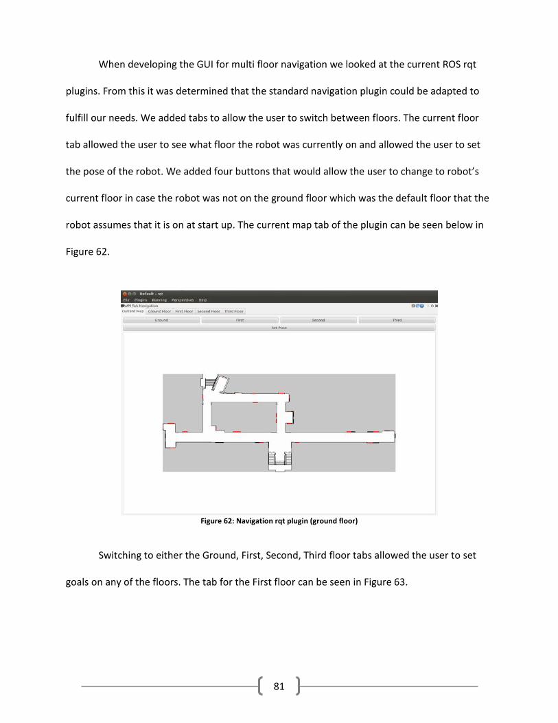
When developing the GUI for multi floor navigation we looked at the current ROS rqt
plugins. From this it was determined that the standard navigation plugin could be adapted to
fulfill our needs. We added tabs to allow the user to switch between floors. The current floor
tab allowed the user to see what floor the robot was currently on and allowed the user to set
the pose of the robot. We added four buttons that would allow the user to change to robot’s
current floor in case the robot was not on the ground floor which was the default floor that the
robot assumes that it is on at start up. The current map tab of the plugin can be seen below in
Figure 62.
Figure 62: Navigation rqt plugin (ground floor)
Switching to either the Ground, First, Second, Third floor tabs allowed the user to set
goals on any of the floors. The tab for the First floor can be seen in Figure 63.
81

Figure 63: Navigation rqt plugin (first floor)
The Ground, Second and Third floor tabs were identical other than the map displayed.
To select a goal the user would click a point, goal point, and drag in the direction the user
wanted the front of the robot to face, goal orientation. Once a goal was selected the robot
would plan a path to the elevator, use the elevator and then set the specified pose as a goal.
The robot also executed successful obstacle avoidance. To do this the robot was treated
as a point while the obstacles were expanded by the radius of the robot. By implementing this
method a path could be found without having to check for collisions in neighboring grid
squares. This process of inflating the obstacles results in a cost map. This cost map can be seen
in Figure 64. The black is the walls and the yellow is detected obstacles, while the turquoise and
purple are inflations from the cost map. If an obstacle appeared in the path of the robot, the
robot would re-plan its path, around the added cost map space, and turn to avoid the obstacle.
If the robot was already too close to the obstacle to turn smoothly, it would stop and rotate in
82

place. Figure 64, Figure 65 and Figure 66 show the actions of the robot when an obstacle is
found in its path.
Figure 64: Robot with clear path
Figure 65: Robot with obstacle in path
Figure 66: Robot with new path around obstacle
The main problem with navigation that was discovered during our tests was due to the
processing limitations of our computer. When all the navigation nodes were running, the
computer’s processing capabilities were maxed out. This caused the computer to sporadically
lock up, occasionally causing nodes to stop running properly.
Finally, the navigation also ended up with an array of ROS packages all launched from a single
launch file in ROS. This launch file can be seen in Appendix B. This Launch file made sure to
connect to the Segway and set it to tractor mode, as well as launch all the pose and
transformation broadcaster, planner and localization nodes, ensuring all the required nodes
were running when trying to navigate.
83

6.0 Discussion The robot was assembled and coded to the best of our ability but some tasks and
designs didn’t turn out the way we would have liked. Here we disucss how the subsystems were
developed and problems encountered and overcome during the process.
6.1 Electrical Design
There were a few aspects of the PCB that did need modifications. First, acrylic covers
were made so that the solder pins on the back of the PCB were not exposed. Also due to the
high force needed to pull apart the connectors, some metal bars were added to aid in
supporting the connectors. They were placed in the holes between the connectors and then
held in place between two acrylic pieces. They reduced the strain on the board when pulling
the connectors out.
When five connectors were connected together the row was hard to pull out in its
current mounting situation. To overcome this we filed down the connectors so that they could
each be pulled out alone. We also spaced the connectors apart when the rails were not full.
This could be solved by replacing the high dent connectors with the equivalent low dent
connectors. It would reduce the need to space them apart and it would allow the user to
interlock the connectors. Since the high dent connectors did take more force to pull apart,
there was more certainty that the connections would hold. For our situation the board had
extra space therefore the spacing out solution worked. The added space on the PCB was
considered beneficial as it allowed us to add both the arm controls and power easily with added
space left over. There was an entire rail not used at the end of our project.
84

Overall, the board was successful. New connectors could be used to possibly make the
board more usable. The acrylic protectors and cover was considered helpful in making sure that
any force applied from the cables being pulled would not affect the PCB.
6.2 Arm Design & Control Any design project has its own set of constraints, and these constraints not only define
the process, but also the final result of the design. In our case, the most significant constraint
was limited budget. Because of our limited available funds, both the design and prototyping
processes were done using SolidWorks. While typical for initial design, using computer-aided
design (CAD) software for the prototyping process has limitations. CAD software driven
prototyping is still a viable option, but not having physical prototypes to work with prevents any
practical testing and leaves any feasibility or function issues ambiguous and up to us to resolve
based on our best judgment.
Once a design was decided upon and parts were obtained, the construction of the arm
progressed relatively according to plan, albeit slower than desired. Because the budget for the
project was limited, extreme care was given to the parts that needed machining, as
replacement stock was very limited and no more could be ordered. Manual machining was used
where deemed appropriate, but parts that required precise cuts were machined using a Haas
CNC Mini Mill.
From a controls perspective, the timeline of the arm shouldn’t have affected the
development of the logic and coding. The logic and coding could have been a developed in
parallel to the construction of the manipulator to make integration at the end a lot easier.
Given the short timeline, the controls were able to be developed enough to provide basic
85

functionality but objection recognition and manipulation occurred, which falls under both
controls and robust manipulator design.
A struggle in code development was an initial choice in microcontroller. The PIC32
microcontroller had plenty of features that were unnecessary given this scope. The late switch
to an Arduino microcontroller meant having to recode the controls, but it also meant less
overhead in setting up the board and pins.
The lack of full implementation of the arm controls is a frustration. Each aspect of the
design was tested previously, before complete integration, but the manipulator as a whole was
not tested. The two-link arm at the end of the four-bar linkage was made functional, but it
lacked the communication to the computer to update its own set-points.
As a whole, the manipulator design did not meet all of the design specifications set out
at the beginning of the project. Budget constraints and development speed played major
factors in this outcome. Despite these setbacks, a strong industrial robotic manipulator was
developed for less than $600.
6.3 Navigation and Software As was mention in section 5.3, the reliability of the robot was not ideal. Although each
aspect of navigation was successfully tested prior to integration, when integrated, aspects of
navigation did not occur at the desired frequencies. This is because the computer could not
handle the processing load.
86

Figure 67: System monitor while the robot was navigating
As shown in Figure 67 above, all of the cores were running at their full capacity. One of
the processes that was most impacted by this processing bottleneck was the amcl node. The
amcl node is responsible for localizing the robots position on the current map using the laser
scanner. This process of localization is supposed to occur after the robot translates or rotates
slightly. However, due to the processing bottleneck, the amcl node could not keep up, resulting
in missed updates to the position. The missed updates often resulted in the laser scanner points
being registered in the wrong location, especially during rotation, as the scan points were
recorded in the locations the robot had been looking as a split second earlier. The biggest
impact of this on navigation was when trying to enter and exit the elevator. As the robot turned
to position its self in front of the elevator doors, the laser scanner points would be offset from
the map by a few degrees. Between the offset scan and the known map the robot saw many
obstacles that were blocking its path. When the elevator doors opened and the path was clear
for the robot to get on, it could not plan a path and the navigation would fail. A person who was
87

assisting the robot could update its pose using the GUI and the robot would then continue
navigation, but this is clearly not a viable option for autonomous navigation. We were able to
minimize the effect of this by not running some of the visualization aspects of ROS, such as
RViz, that were only necessary for debugging purposes. The only problem with turning RViz off
was that if something did go wrong, the debugging process was much harder as there was less
information available to us.
Another result of the processing bottleneck was when travelling between floors. Once
the robot was on the elevator to go to a new floor, the map would change from the floor it was
on the floor it was going. When the map changed the robot would sometimes start to rotate.
This was a result of the new pose of the robot not set fast enough and therefore the robot
would try to navigate toward the goal position which was behind the robot relative to the new
map. When the robot rotated, again amcl could not always keep up and the robot would alter
the laser scan to no longer be where the doors would be. This again causes navigation issues
because the doors would open and the robot would not see a path out of the elevator or the
rotation could cause the robot to no longer be able to see the LED screen to know which floor
the elevator was at.
In order to reduce the load on the computer, a second computer was attempted to be
used. The second computer was connected over wifi to the router the main computer was
connected to over Ethernet. This did not show much in any improvement in the reliability of the
system. This was partly due to the speed of the wireless network which limited, much like the
processing power bottleneck, how fast certain nodes could update. This meant the benefit of
running on multiple computers was limited and did not increase the reliability of the system by
88

much but the processing load on the computer was slightly reduced. There may have been
more of a performance gain if we could have connected over Ethernet but the second
computer we were testing with did not have an Ethernet port, it only had wifi. Since the
performance increase from a second computer over wifi was minimal, it was determined that
the use of the single computer would be more effective.
Without the Kinect in use, the robot could not determine if the floor, the elevator was
on, is the floor at which the robot was supposed to get off. As soon as the doors would open
and there was a path the robot would have exited the elevator. Therefore, it was important to
make sure that the robot had some way to determine if it was the correct floor. The image
matching solved this issue. Due to the poor lighting conditions in the elevator, there was some
concern that the templates would not be visible to the Kinect or would not be matched
correctly, for example the second floor template matching to the third floor template. During
our testing we discovered that the templates could be matched incorrectly however, the
frequency of such errors was very small and the mismatched template would never match as
well as the comparison between the same numbers. To minimize the effect of mismatched
templates we required several consecutive matches before a match to the desired floor was
taken to be accurate. We also only check for the desired floor that we wish to get off the
elevator to reduce the number of templates we were trying to match at once which should
reduce mismatched with floors that we aren’t looking for. This also allows us to perform the
template matching faster for the desired floor than we could if we were trying to track the
elevator by matching all the templates at once. With these rules in place the template matching
performed extremely well, always correctly identifying when the elevator reached the desired
89

floor. One benefit of this node is that it is easily adapted to other elevators that have a LED or
other type of screen and template pictures of each number is taken before execution.
Also the caster wheel caused some issues with the robot when turning. This was due to
the nature of the castor wheel and the rugged floors. The castor wheel supported the weight of
the gel cell battery and would therefore be harder to move. If the caster was facing straight and
the robot wanted to turn in place the robot would have issues because of the force needed to
swivel the wheel.
Considering all of this, the robot could navigate autonomously and performed quite
well. With a few changes to the hardware and design of the platform, this system has the
potential to be a very robust autonomous navigation platform.
90

7.0 Conclusions and Recommendations As was mentioned earlier, the computer would max out all four processing cores while
the navigation ROS nodes were running. Therefore, our first recommendation is a PC with more
processing capabilities for the robot. A computer with a faster processor is needed so that all of
the nodes can run at the desired frequencies. Another aspect to take into consideration is
power consumption; if a new computer is purchased, one with a lower power consumption and
integrated graphics would be desired. Also in order to store the all of the log information a
larger solid state drive would also be recommended. Another option is to get a second PC and
distribute the loads.
In order to distribute the processing load multiple computers could be used. This could
have worked for us if the router had a faster wifi connection. The laptop used to distribute the
load did not have an Ethernet port therefore no tests were done with distributed load over
Ethernet. Trying to distribute the load over wifi connection showed very little performance
change. To address this we recommend a better Wi-Fi router or tests with distributing the
processing nodes over Ethernet. This would allow for the distribution of the processing load to
be more effective.
Another recommendation is to improve the camera. Right now the camera must tilt up
to see the needed workspace while navigating and then tilt back down to see the arm
workspace. A camera with a larger field of view and better resolution would make tele-
operated control of the arm easier and the image quality would improve. Image matching
would also be easier as well as more accurate as the number of comparisons would increase
91

with higher resolution. A new version of the Kinect is going to be released by Microsoft that
would have fulfilled these requirements, but the sensor was not available before the conclusion
of this project.
After the code for the Segway was developed, it was sent to Segway Inc. for them to
review. One improvement that was suggested was to implement a multi-threaded interface
with the Segway base through Ethernet. A multithreaded approach would have allowed us to
send commands and receive feedback at different rates solving the issue of not getting
feedback when no command was sent, as seen in our single threaded approach.
To address the issue of the robot turning in the elevator, the maps could be aligned by
the elevator. This way, when the robot is travelling in the elevator its pose would remain the
same in each map. This would solve the issue mentioned before of having the robot move
around the elevator when travelling between floors. By aligning the maps by the position of the
elevator, the robot would no longer be confused for a few seconds as the map was changing
and the pose of the robot updating.
Full multi-waypoint navigation is recommended to round out the navigation. Once a
user has selected a location and object to retrieve, the robot should be able to navigate to the
goal, find and retrieve the object, and return to the user. This would make the platform a fully
assistive mobile manipulation platform.
The first recommendation regarding the arm design would be to fully implement the
robotic manipulator. We feel the design has potential to be a successful implementation of a
manipulator given the budget and time constraints. The design could use better manufacturing
92

and design at the joints to minimize deflection and deformation over time. If the controls were
fully implemented to move the arm, the functionality of the overall robot would increase
dramatically.
Once the implementation of the arm was complete, image recognition would be the
next step. Moving from a teleoperated manipulator to a fully autonomous manipulator is the
next recommendation. This would require research into object recognition using a Kinect and
learning algorithms to pick out new objects as a user needed them.
The final recommendation would be to implement transportation logic for objects. Once
an object can be recognized and picked up, there will need to be some design of how to carry
the object to the user. It would consume a lot of power if the manipulator were to be running
for the duration of the transport. Maybe this would involve designing a platform to store the
objects on while navigating back to the user.
Long-term recommendations for the research platform include object retrieval and
other assistive applications. This application would be to allow the user to ask for an object
without knowing its location. The user, for example, could ask for a cup and the robot would
know where the cup was and set its own goals. This would allow the robot to navigate
autonomously without the need of set goals from the user or tele-operation of the arm. Voice
control of the robot would allow for user with a higher degree of injuries to ask for objects and
receive them.
93

References Altium. (2014). Altium Designer (Version 10): Altium. Retrieved from http://www.altium.com/
Automation, F. I. f. M. E. a. (2013). Care-O-bot 3. Retrieved 9/9/2013, 2013, from
http://www.care-o-bot.de/en/care-o-bot-3.html
Bayle, B., Fourquet, J.-Y., & Renaud, M. (2003). Manipulability of Wheeled Mobile
Manipulators: Application to Motion Generation. The International Journal of Robotics
Research, 22(7-8), 565 - 581. doi: 10.1177/02783649030227007
Bchretien. (2014). MoveIt! , from https://aur.archlinux.org/packages/ros-hydro-rqt-moveit/
Beardmore, R. (2011). Simple linkages. Retrieved 11/0713, 2013, from
http://www.roymech.co.uk/Useful_Tables/Mechanics/Linkages.html
Borst, C., Wimbock, T., Schmidt, F., Fuchs, M., Brunner, B., Zacharias, F., . . . Hirzinger, G. (2009).
Rollin' Justin - Mobile platform with variable base. Paper presented at the IEEE
International Conference on Robotics and Automation, Kobe.
http://ieeexplore.ieee.org/xpl/articleDetails.jsp?arnumber=5152586
Computing, M. E. S. o. (2013). Inverse Kinematics for Position. Retrieved 04/20/2014, 2014,
from http://www.eng.utah.edu/~cs5310/chapter5.pdf
Corperation, D. S. S. (2012). SolidWorks (Version 2012): Dassault Systemes.
Correa, D. S. O., Sciotti, D. F., Prado, M. G., Sales, D. O., Wolf, D. F., & Osório, F. S. (2012, 2012).
Mobile robots navigation in indoor environments using kinect sensor. Paper presented at
the Second Brazilian Conference on Critical Embedded Systems.
Garage, W. (2014). PR2. 2014, from http://www.willowgarage.com/pages/pr2/overview
94

Gerig, G. (2012). Image Rectification (Stereo). http://www.sci.utah.edu/: University of Utah
Scientific Computing and Imaging Institute.
Graf, B., Hans, M., & Schraft, R. D. (2004). Care-O-bot II—Development of a Next Generation
Robotic Home Assistant. Autonomous Robots, 16(2), 193-205. doi:
10.1023/B:AURO.0000016865.35796.e9
Harris, T. (2002). How Robots Work. Retrieved 10/23/2013, 2013, from
http://science.howstuffworks.com/robot2.htm
Hokuyo. (2009). URG-04LX-UG01. 2014, from https://www.hokuyo-
aut.jp/02sensor/07scanner/urg_04lx_ug01.html
Jenkel, T., Kelly, R., & Shepanski, P. (2013). Mobile Manipulation for the KUKA youBot Platform.
(Bachelor of Science), Worcester Polytechnic Institute, Worcester, MA.
KUKA. (2013). youBot Store. from http://www.youbot-store.com/
LeBlanc, N., Patel, K., & Rashid, S. (2012). Guest Orientation, Assistance, & Telepresence
(G.O.A.T.) Robot. (Bachelor of Science), Worcester Polytechnic Institute, Worcester, MA.
Li, Y., & Ruichek, Y. (2013). Building Variable Resolution Occupancy Grid Map from Stereoscopic
System - a Quadtree based Approach. Paper presented at the IEEE Intelligent Vehicles
Symposium, Gold Coast, Australia.
Lipsett, R. (2013). Designfax – Technology for OEM Design Engineers. Retrieved 10/12/13,
2013, from http://www.designfax.net/cms/dfx/opens/article-view-
dfx.php?nid=4&bid=239&et=featurearticle&pn=06
95

Luostarinen, R., Manner, J., Maatta, J., & Jarvinen, R. (2010, Oct. 31 2010-Nov. 3 2010). User-
centered design of graphical user interfaces. Paper presented at the Military
Communications Conference.
MathWorks. (2014). Computer Vision System Toolbox: Stereo Vision. from
http://www.mathworks.com/products/computer-
vision/examples.html?file=/products/demos/shipping/vision/videostereo.html
Miran, G., & Mislav, G. (2010, 15-17 September, 2010). Accomplishments and Challenges of
Computer Stereo Vision. Paper presented at the 52nd International Symposium ELMAR-
2010, Zadar, Croatia.
Products, A. P. (2014). Powerpole Connectors. Retrieved 11/07/2013, 2013, from
http://www.andersonpower.com/products/singlepole-connectors.html
Riisgaard, S., & Blas, M. R. (2003). SLAM for Dummies. A Tutorial Approach to Simultaneous
Localization and Mapping, 22, 1-127.
Robots, S. o. (2013). Robot Arm Tutorial. Retrieved 10/09/13, 2013, from
http://www.societyofrobots.com/robot_arm_tutorial.shtml#robot_workspace
Stentz, A. (1994, 1994). Optimal and efficient path planning for partially-known environments.
Paper presented at the IEEE International Conference on Robotics and Automation.
Stentz, A. (1995, 1995). The focussed D^* algorithm for real-time replanning. Paper presented
at the International Joint Conference on Artificial Intelligence.
Thomas, D., Scholz, D., & Blasdel, A. (2014). rqt. 2014, from http://wiki.ros.org/rqt
96

Appendix A: SolidWorks SimulationXpress Results
97

98

99

100

101

102

Figure 68: SolidWorks simulation of coupler horizontal linkage mount (Corperation, 2012)
103

104

105

106

107

108

109

Figure 69: SolidWorks simulation of final arm link 1 (Corperation, 2012)
110
111

112

113

114

115

116

Figure 70: SolidWorks simulation of T-slotted extrusion 5in (Corperation, 2012)
117

118

119

120

121

122

123

Figure 71: SolidWorks simulation of Wrist 3.0 (Corperation, 2012)
124

Appendix B: Launch File Navigation: move.launch <launch> <include file="$(find wpi_map)/launch/maps.launch"/> <node pkg="wpi_segway_rmp" type="rmp_exchange.py" name="rmp_exchange"/> <node pkg="move_base" type="move_base" name="move_base"> <param name="base_global_planner" value="navfn/NavfnROS"/> <param name="base_local_planner" value="base_local_planner/TrajectoryPlannerROS"/> <param name="controller_frequency" value="20.0"/> <param name="planner_patience" value="180.0"/> <param name="conservative_reset_dist" value="10.0"/> <rosparam file="$(find wpi_segway_nav)/navfn_params.yaml" command="load" /> <rosparam file="$(find wpi_segway_nav)/base_local_planner.yaml" command="load" /> <rosparam file="$(find wpi_segway_nav)/costmap_common_params.yaml" command="load" ns="global_costmap" /> <rosparam file="$(find wpi_segway_nav)/costmap_common_params.yaml" command="load" ns="local_costmap" /> <!-- Load global navigation specific parameters --> <rosparam file="$(find wpi_segway_nav)/local_costmap_params.yaml" command="load" /> <rosparam file="$(find wpi_segway_nav)/global_costmap_params.yaml" command="load" /> </node> <include file="$(find wpi_segway_pose)/launch/tf_frames.launch" /> <include file="$(find wpi_segway_nav)/launch/amcl_diff.launch" /> <node pkg="wpi_segway_nav" type="cmd_vel_converter.py" name="cmd_vel_converter"/> <node pkg="wpi_segway_nav" type="scan_filter.py" name="scan_filter"/> <include file="$(find wpi_segway_nav)/launch/wpi_hokuyo.launch" /> <node pkg="wpi_segway_nav" type="multi_floor_planner.py" name="multi_floor_planner" output="screen"/> <include file="$(find freenect_launch)/launch/examples/freenect-registered-xyzrgb.launch" /> <node pkg="wpi_nav_image" type="elevator_recog.py" name="elevator_recog"/> <include file="$(find wpi_arm)/launch/camera_frame.launch" /> </launch>
125

Appendix C: Arm Control Code void loop() { if(FLAG) { Setpoint_S = S_STANDBY; Setpoint_E = E_STANDBY; Setpoint_W = W_STANDBY; } else { // for now...til serial is setup Setpoint_S = S_STANDBY; Setpoint_E = E_STANDBY; Setpoint_W = W_STANDBY; } Input_S = analogRead(SHOULDER_POT_PIN); Input_E = analogRead(ELBOW_POT_PIN); Input_W = analogRead(WRIST_POT_PIN); if(feedback == 1){ // getCommands(); feedback = 0; } switch(STATE) { // this is where the 2-link arm is in STANDBY and the shoulder moves case 0: // save read setpoints to temp vars; save standbys to setpts; E_temp = Setpoint_E; W_temp = Setpoint_W; Setpoint_E = E_STANDBY; Setpoint_W = W_STANDBY; break; // this is the state where the shoulder should be in position, and the 2-link arm can move into position case 1: Setpoint_E = E_temp; Setpoint_W = W_temp; break; // this is meant to actuate the gripper, but we may be able to just directly actuate that case 2:
126

break; // have not set default case default: break; } // compute the PID errors and save to *output for each joint PID_SHOULDER.Compute(); PID_ELBOW.Compute(); PID_WRIST.Compute(); // actuate motors if(Output_S < -10) { digitalWrite(SHOULDER_A_PIN,LOW); digitalWrite(SHOULDER_B_PIN,HIGH); //===> turns the shoulder *LEFT* analogWrite(S_EN,(-1*Output_S)); } else { digitalWrite(SHOULDER_A_PIN,HIGH); digitalWrite(SHOULDER_B_PIN,LOW); //===> turns the shoulder *RIGHT* analogWrite(S_EN,Output_S); } //====== Actuate the ELBOW ======== if(Output_E < -10) { digitalWrite(ELBOW_A_PIN,LOW); digitalWrite(ELBOW_B_PIN,HIGH); //===> turns the elbow *LEFT* analogWrite(E_EN,(-1*Output_E)); } else if(Output_E > 10) { digitalWrite(ELBOW_A_PIN,HIGH); digitalWrite(ELBOW_B_PIN,LOW); //===> turns the elbow *RIGHT* analogWrite(E_EN,Output_E); } else { digitalWrite(ELBOW_A_PIN,HIGH); digitalWrite(ELBOW_B_PIN,HIGH); //===> Brakes the ELBOW analogWrite(E_EN,LOW);//---coasting } //====== Actuate the WRIST ======== if(Output_W < -10) { digitalWrite(WRIST_A_PIN,LOW);
127

digitalWrite(WRIST_B_PIN,HIGH); //===> turns the wrist *LEFT* analogWrite(W_EN,(-1*Output_W)); } else if(Output_W > 10) { digitalWrite(WRIST_A_PIN,HIGH); digitalWrite(WRIST_B_PIN,LOW); //===> turns the wrist *RIGHT* analogWrite(W_EN,Output_W); } else { digitalWrite(WRIST_A_PIN,HIGH); digitalWrite(WRIST_B_PIN,HIGH); //===> Brakes the WRIST analogWrite(W_EN,LOW);//---coasting } // send current pot values back /* Serial.write(blah_blah_blah); Serial.write(blah_blah2); Serial.write(blah1); */ }
128