WORKING PAPER NO. 108

INDIA’S POLICY STANCE ON RESERVES AND THE CURRENCY

ILA PATNAIK

SEPTEMBER 2003

INDIAN COUNCIL FOR RESEARCH ON INTERNATIONAL ECONOMIC RELATIONS

Core-6A, 4th Floor, India Habitat Centre, Lodi Road, New Delhi-110 003

Foreword

India’s reserves have been growing since the external reforms of 1991-2 and 1992-3. There was a minor interruption after the Asian crises as India borrowed money abroad through the mechanism of the Resurgent India Bonds (RIBs), at a relatively high rate of interest. The pace of reserve accumulation has picked up since then with an addition of $25 billion to reserves in 2002-3.

Reserve accumulation can be part of a deliberate move to build up reserves as it was in

1991-92 and in 1992-93 after reserves had sunk to one month of import during the BOP crises. Reserves can also be the outcome of exchange rate management of new developments on the external sector. For instance, an unprecedented $ 6 billion of FII inflow came in over a 12 month period from October 1993 to September 1994. This unprecedented inflow was the result of the opening of the economy to equity flows coupled with market reforms and represented a stock adjustment of the global equity portfolio. Reserves accumulated during this period because of a deliberate decision to curb appreciation of the rupee through RBI purchase of excess inflows. An earlier ICRIER paper argued that this was part of an assymmetric exchange rate management policy that was more benign towards depreciation of the rupee in response to adverse policy developments but restrained appreciation in response to positive shocks such as equity flows representing a stock adjustment. There was also a declared RBI policy since the introduction of market related exchange in 1992, that the RBI would intervene to dampen day to day volatility in the exchange market.

Empirical literature on currency regimes suggests that from August 1991 to June 1995

India’s currency regime is best described as a de facto peg to the US dollar, while from then to end 2001 it was a de facto crawling peg. This conclusion is consistent with the objective of dampening volatility. In our view it would also be consistent with the asymmetric exchange management hypothesis, if the balance of payments resulted in an excess of capital inflows over the current account deficit during the first period and a deficiency during the second. According to this hypothesis the rupee would not be allowed to appreciate in the first situation and reserves would accumulate. In contrast, in the second situation, reserves would be relatively stable while the rupee would be allowed to trend downwards (depreciate). Further research is however required to resolve this issue for the 1992-3 to 1996-7 period.

The analysis of the paper is focussed on the period since the Asian crisis. It argues that a

clear and well articulated official position on India’s currency regime is not available. It examines the various potential reasons for reserve accumulation emerging from the statements of officials and official committees to show that reserve accumulation is the outcome of a currency regime whose main objective is to deliver low volatility of the nominal exchange rate. . Excessive currency accumulation is seen to be an outcome of this regime. The paper shows that during the past few years the rupee appears to be a de facto peg to the US dollar. Thus the situation seems to have reverted, at least since 2002, to that prevailing between 1992 to 1995.

The paper makes a contribution to the current debate on India’s currency regime and

reserve policy, issues that have greater significance with the opening of the capital account and the new challenges it poses for interest rate policy in India.

Arvind Virmani Director & Chief Executive

ICRIER September 2003

India’s policy stance on reserves and the currency

Ila Patnaik∗

ICRIER, New Delhiila@icrier.res.in

http://openlib.org/home/ila

September 4, 2003

Abstract

Over the last decade, India engaged in substantial liberalisationon the current account and the capital account. At the same time, afully articulated policy framework defining the currency regime is notknown in the public domain. In this paper, we seek to characterise thenature of the currency regime, in the period after the Asian crisis. Thisis closely linked to better understanding the phenomenon of reservesaccumulation of the recent years. Our results suggest that the mainfocus of the currency regime has been to deliver a low volatility ofthe nominal exchange rate. The rupee appears to be a de facto pegto the USD. In the last one year, reserves accumulation cannot beexplained by insurance motivations; it seems to be a passive side effectof maintaining the currency regime.

∗This paper grew out of conversations with Ajay Shah. The views in this paper aremine and not of my employers. I am grateful to Arvind Virmani, Shankar Acharya,the Macrists, Ashok Lahiri, A. Prasad, and Gomez Pineda Javier Guillermo for usefuldiscussions, to R. K. Pattnaik, CMIE and Indian Quotation Systems for help on data,and Susan Thomas and Tirthankar Patnaik for help on statistical testing.

1

Contents

1 Introduction 3

2 India’s reserves buildup 4

3 Reserves adequacy 63.1 Conceptual issues . . . . . . . . . . . . . . . . . . . . . . . . . 63.2 Indian experience . . . . . . . . . . . . . . . . . . . . . . . . . 7

4 Exchange rate management 104.1 Real versus nominal . . . . . . . . . . . . . . . . . . . . . . . 104.2 Understanding a currency regime . . . . . . . . . . . . . . . . 104.3 Official position . . . . . . . . . . . . . . . . . . . . . . . . . . 11

5 Methodology for characterising currency regime 125.1 Exchange rate flexibility . . . . . . . . . . . . . . . . . . . . . 135.2 Volatility . . . . . . . . . . . . . . . . . . . . . . . . . . . . . 145.3 Multi currency model . . . . . . . . . . . . . . . . . . . . . . 155.4 Measures of market efficiency . . . . . . . . . . . . . . . . . . 155.5 Did policy target the REER or NEER? . . . . . . . . . . . . 16

6 Indian evidence 176.1 Currency flexibility . . . . . . . . . . . . . . . . . . . . . . . . 186.2 Evidence from Reinhart & Rogoff, 2002 . . . . . . . . . . . . 196.3 Volatility . . . . . . . . . . . . . . . . . . . . . . . . . . . . . 196.4 Regression based approach . . . . . . . . . . . . . . . . . . . . 216.5 Market efficiency . . . . . . . . . . . . . . . . . . . . . . . . . 236.6 Is the REER or the NEER being targeted? . . . . . . . . . . 26

7 Conclusion 28

2

1 Introduction

India has experienced a breathtaking increase in the stock of foreign ex-change reserves, from a near-zero level in 1991 to $80 billion in May 2003.In particular, in the period after the Asian crisis, countries all over Asiahave rapidly built up reserves. In this paper, we seek to obtain some in-sights on the factors shaping this accretion of reserves. This question isinnately closely related to that of characterising the currency regime.

Reserves accretion can occur owing to a desire to hold reserves as ‘insurance’.It is widely believed that the cost of holding reserves is a necessary ‘insurancepremium’, that should be paid by a developing country that seeks to safelyharness the benefits of globalisation. As an alternative hypothesis, reservesaccretion or depletion can occur as a passive consequence of exchange ratepolicy.

We document a variety of metrics of reserves adequacy that have been pro-posed, in seeking to identify the level of reserves that are desirable in orderto achieve insurance goals. We find that by March 2002, these metrics weresubstantially satisfied. Yet, India went on to add $25 billion in reserves inthe period after March 2002. This suggests that ‘reserves as insurance’ isnot a hypothesis that adequately explains the observed facts.

RBI has not released documents defining the rules through which the cur-rency regime operates. Hence, we must make inferences based on data inorder to understand the currency regime. Last year, two papers on thisquestion highlighted the limited exchange rate flexibility of the INR-USDexchange rate (Calvo & Reinhart 2002, Reinhart & Rogoff 2002). Calvo& Reinhart observe that currency flexibility in India has not changed since1979. Reinhart & Rogoff apply a data-driven algorithm for the classificationof the de facto currency regime across a large database of countries. Theyclassify India as a “de facto crawling peg to the US dollar”.

In this paper, we exploit a broad range of empirical strategies, for ob-taining insights into the nature of the currency regime. These include ameasure of exchange rate flexibility, regression models based on multiplecross-currency exchange rates, measures of market efficiency, and testablepropositions about cross-currency volatility. Our broad finding is that inthe period following the Asian crisis, the rupee appears to be a de facto pegto the US dollar.

One competing hypothesis is that policies targeted the reer or the neer.We argue that if the reer or the neer were targeted, then they shouldexhibit low volatility. Instead, we find that they exhibit greater volatilitythan the nominal INR/USD rate. This suggests that reer targeting wasnot the goal of policy.

3

Figure 1 Growth of foreign exchange reserves

1990 1995 20000

20

40

60

80

100

Bill

ion

USD

Foreign currency reservesExternal debt

In summary, we find that India’s policy stance on reserves and the currencyis primarily one of exchange rate management on the INR/USD exchangerate which seeks to obtain low volatility of rate. Fluctuations of reservesappear to be a side effect caused by the pursuit of goals of currency policy.

The remainder of this paper is organised as follows. Section 2 shows thefamiliar empirical facts about India’s experience with reserves accretion,and summarises the competing hypotheses which could serve as explana-tions. Section 3 explores the hypothesis that the reserves accretion of recentyears was a consequence of policies focused on reserves adequacy. Section4 describes the conceptual backdrop of ‘characterising a currency regime’.Section 5 shows the methodologies that we will exploit in characterisingthe currency regime. Section 6 applies these methodologies to Indian data.Finally, Section 7 concludes the paper.

2 India’s reserves buildup

The build-up of foreign exchange reserves in India has been a major phe-nomenon in the post-1991 period. Figure 1 shows the familiar time-series,which shows that reserves rose sharply from $20 billion in 1995 to $75 billionin 2002 - an increase of roughly 10% of GDP. Starting from near-zero levelsin 1991, India is now the seventh largest holder of international reserves inthe world. Figure 1 highlights the fact that while reserves accretion wasoccasionally done using debt inflows, for the major part, it was associated

4

with stable external debt.

In 2002-03 alone, India added roughly $20 billion to her forex reserves.This scale of addition to reserves is a unique phenomenon when comparedwith India’s historical experience, and invites further exploration (Ranade& Kapur 2003).

In general, growth in reserves can happen owing to asset management of thereserves portfolio, or owing to interventions by the central bank.1 Intuitively,we may expect returns of a few percent in reserves management. If a countryhas $100 billion in reserves, then changes in reserves of a few billion dollarscan occur owing to fluctuations in asset prices.

In India’s case, some of the increase in reserves during 2002-03 was the resultof the appreciation of the Euro and the Japanese Yen against the USD.However, foreign exchange intervention by the RBI was the main cause ofthe build up of reserves during 2002-03. According to RBI data, out of$20.8 billion that were added to reserves during April-December 2002, $3.8billion were added because of valuation changes, while $13.3 billion representcapital inflows and 3.7 the current account surplus.

There are broadly two competing explanations for a phenomenon of rapidaddition to reserves:

Reserves as a goal of policy It could be the case that India added reserves as aconsequence of reserves policy. That is, India had certain thought out targetsfor the minimum required level of ‘reserves as insurance’, and was trying torapidly reach this target level.

Reserves as a side effect of currency policy Alternatively, buying and sell-ing reserves could have been passive side effects of currency policy. Reserveswould go up when RBI intervened to push the price of the INR down, andvice versa.

Thus, as an alternative to the hypothesis that India has followed a policyof achieving a desired level of reserves as ‘insurance’, the major competingexplanation is one where RBI has been primarily focused on exchange ratemanagement, and reserves have fluctuated passively as a response to theexigencies of RBI’s trading on the currency market. In this paper, we seekto obtain some insights on the importance of these competing explanationsin understanding India’s post-1991 experience.

This is about disentangling cause and effect. The unambiguous stylisedempirical fact is that reserves grew dramatically, and the INR was weak.

1In addition, reserves can also change owing to repayment of external debt. However,this has been relatively unimportant in explaining the time-series volatility of reserves inIndia.

5

We seek to understand whether reserves rose as a consequence of currencypolicy, or whether the INR was weak as a consequence of reserves policy.

The key intuition that we employ, in understanding variables which aretargeted, as opposed to variables which are either instruments of policy orare side effects, is based on interpreting volatility. If reserves were targeted,then a country would experience first reserves volatility in getting to thetarget, but then experience low volatility of reserves. Other variables (suchas external debt, exchange rates, money supply and interest rates) would bevolatile in the process of achieving targets for reserves. Conversely, if theexchange rate were targeted, then other variables (such as reserves, moneysupply, interest rates) would be relatively volatile while exchange rates wouldbe stable.

3 Reserves adequacy

3.1 Conceptual issues

If reserves are held as insurance, how large do they need to be? Whatis an appropriate ‘target’ for reserves? In the literature on ‘reserves asinsurance’, there are four kinds of measures which have been proposed forjudging reserves adequacy :

Trade based measures Trade based measures focus on the current account. Re-serves are generally thought to be adequate when they cover six months ofmerchandise imports.2

Debt based measures Trade-based measures of reserves adequacy have beencriticised, since they pay no heed to obligations owing to the capital account.

Debt based measures focus on the capital account only, and measure theability of reserves to support debt servicing. If access to capital markets islimited, or if the country depends heavily on short term debt, then such mea-sures indicate the level of risk in the event of sudden movements in capital,or changes in the availability of capital.

Liquidity based measures Liquidity based measures focus on the extent to whichreserves can fund all capital account liabilities. In April 1999, Pablo Guidotti,then the Deputy Finance Minister of Argentina, suggested that emergingmarket economies should maintain usable foreign exchange reserves thatcover debt requirements for atleast a year. Projecting a current accountdeficit and short term debt provides a measure of new borrowing that may

2Amongst the east Asian countries which experienced a crisis in 1997, reserves wentup from 3 months of imports in 1997 to 8 months of imports cover in 1999 (Hawkins &Turner 2000).

6

be required by a country. Guidotti proposed that reserves should be adequateto require no new borrowing for a year.

Alan Greenspan extended this ‘Guidotti rule’, suggesting a ’liquidity at risk’measure that also takes into account a range of possible scenarios for ex-change rates, commodity prices, credit spreads etc, and takes cognisance ofderivatives such as foreign currency bonds with embedded options.3

This has been dubbed the ’Greenspan rule’, and it suggests that a countryshould hold the level of reserves required to ensure no borrowing requirementsover a horizon of one year with a 95% probability.

Money-based measures Money based measures focus on the extent to which acountry has a domestic currency which is backed by foreign exchange. Thesemeasures include ratios such as reserves to broad money, or reserves to basemoney, which provide a measure of potential for resident based capital flightfrom the currency. To defend a currency peg, the monetary authorities onlyneed enough resources to buy back the high powered monetary base, equal todeposits at the central bank plus currency. In practice a central bank wouldnot need to buy up the entire base to repel any speculative attack (Obstfeld& Rogoff 1995).

East Asian countries such as China, Taiwan, Korea, Singapore and HongKong are prominent in holding large reserves today. It can be argued thatin the period after the Asian crisis, they felt that the insurance motiva-tion demanded a higher level of reserves. However, Aizenman & Marion(2002) find that a model explaining ‘demand for reserves’, based on datafor 125 countries from 1980 onwards, under-predicts the reserves holdings ofthese nations in the period after the 1997 crisis. An alternative explanationis that of Calvo & Reinhart (2002), who suggest that a large number ofcountries are holding a high level of reserves because they continue to haveextremely limited exchange rate flexibility, even though their exchange rateis ostensibly floating.

3.2 Indian experience

In 1991 India had gone down to reserves covering two weeks of imports.Hence, until 1993-94, there was a strong focus upon reserves adequacy mea-sured by months of import cover.

The High Level Committee on Balance of Payments, 1993, chaired by Dr. C.Rangarajan, recommended that the RBI should target a level of reseves thattook into account liabilities that may arise for debt servicing, in addition toimports of three months.

3This is derived from a speech Currency reserves and debt, by Alan Greenspan, at the‘World Bank Conference on Recent Trends in Reserves Management’, Washington, D.C.,1999, http://www.federalreserve.gov/boarddocs/speeches/1999/19990429.htm

7

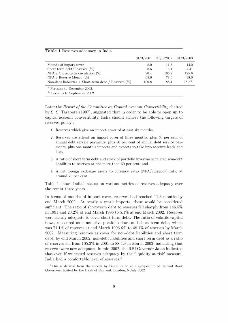
Table 1 Reserves adequacy in India

31/3/2001 31/3/2002 31/3/2003

Months of import cover 8.0 11.3 14.0Short term debt/Reserves (%) 8.6 5.1 4.4∗

NFA / Currency in circulation (%) 90.4 105.2 125.6NFA / Reserve Money (%) 65.0 78.0 98.0

Non-debt liabilities + Short term debt / Reserves (%) 100.8 88.4 78.5#

∗ Pertains to December 2002.# Pertains to September 2002.

Later the Report of the Committee on Capital Account Convertibility chairedby S. S. Tarapore (1997), suggested that in order to be able to open up tocapital account convertibility, India should achieve the following targets ofreserves policy :

1. Reserves which give an import cover of atleast six months,

2. Reserves are atleast an import cover of three months, plus 50 per cent ofannual debt service payments, plus 50 per cent of annual debt service pay-ments, plus one month’s imports and exports to take into account leads andlags,

3. A ratio of short term debt and stock of portfolio investment related non-debtliabilities to reserves at not more than 60 per cent, and

4. A net foreign exchange assets to currency ratio (NFA/currency) ratio ataround 70 per cent.

Table 1 shows India’s status on various metrics of reserves adequacy overthe recent three years.

In terms of months of import cover, reserves had reached 11.3 months byend March 2002. At nearly a year’s imports, these would be consideredsufficient. The ratio of short-term debt to reserves fell sharply from 146.5%in 1991 and 23.2% at end March 1996 to 5.1% at end March 2002. Reserveswere clearly adequate to cover short term debt. The ratio of volatile capitalflows, measured as cumulative portfolio flows and short term debt, whichwas 71.1% of reserves at end March 1996 fell to 48.1% of reserves by March2002. Measuring reserves as cover for non-debt liabilities and short termdebt, by end March 2002, non-debt liabilities and short term debt as a ratioof reserves fell from 105.2% in 2001 to 88.4% in March 2002, indicating thatreserves were now adequate. In mid-2002, the RBI Governor Jalan indicatedthat even if we tested reserves adequacy by the ‘liquidity at risk’ measure,India had a comfortable level of reserves.4

4This is derived from the speech by Bimal Jalan at a symposium of Central BankGoverners, hosted by the Bank of England, London, 5 July 2002.

8

Figure 2 Net purchase of dollars by RBI

-10000

-5000

0

5000

10000

15000

20000

Jan 00Jan 00 Jan 01Jan 01 Jan 02Jan 02 Jan 03Jan 03

Net

RB

I tra

ding

(Rs.

cro

re)

Net purchase of dollars

In summary, most indicators of reserve adequacy showed that by 31 March2002, India had ‘adequate’ foreign exchange reserves, when focusing uponthe ‘insurance’ motivation for holding reserves. This raises the question ofhow we can explain the last $20 billion accreted into reserves, which tookplace in the latest year, i.e. from 1 April 2002 to 31 March 2003. As Figure2 shows, the net purchase of dollars by RBI in the foreign exchange marketdid not slow down over 2000-02.

The extent of debt inflows over the 1990s gives us some insight about theextent to which India was following an active reserves policy. If reservesof $75 billion had been targeted, then we might have expected a greateraddition to debt to reach that target. However, growth in reserves after2000-01 were not debt creating (see Table 2).

In a recent article, Kapur & Patel (2003) argue that India’s reserves accre-tion, which cannot be explained in terms of the metrics of reserves adequacyas shown above, can be attributed to domestic fiscal problems. They arguethat India’s accumulation of reserves is an expression of concern on the partof policy makers owing to the fiscal difficulties that India faces.

9

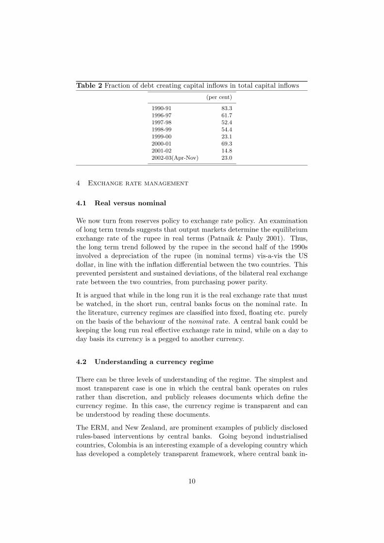
Table 2 Fraction of debt creating capital inflows in total capital inflows

(per cent)

1990-91 83.31996-97 61.71997-98 52.41998-99 54.41999-00 23.12000-01 69.32001-02 14.82002-03(Apr-Nov) 23.0

4 Exchange rate management

4.1 Real versus nominal

We now turn from reserves policy to exchange rate policy. An examinationof long term trends suggests that output markets determine the equilibriumexchange rate of the rupee in real terms (Patnaik & Pauly 2001). Thus,the long term trend followed by the rupee in the second half of the 1990sinvolved a depreciation of the rupee (in nominal terms) vis-a-vis the USdollar, in line with the inflation differential between the two countries. Thisprevented persistent and sustained deviations, of the bilateral real exchangerate between the two countries, from purchasing power parity.

It is argued that while in the long run it is the real exchange rate that mustbe watched, in the short run, central banks focus on the nominal rate. Inthe literature, currency regimes are classified into fixed, floating etc. purelyon the basis of the behaviour of the nominal rate. A central bank could bekeeping the long run real effective exchange rate in mind, while on a day today basis its currency is a pegged to another currency.

4.2 Understanding a currency regime

There can be three levels of understanding of the regime. The simplest andmost transparent case is one in which the central bank operates on rulesrather than discretion, and publicly releases documents which define thecurrency regime. In this case, the currency regime is transparent and canbe understood by reading these documents.

The ERM, and New Zealand, are prominent examples of publicly disclosedrules-based interventions by central banks. Going beyond industrialisedcountries, Colombia is an interesting example of a developing country whichhas developed a completely transparent framework, where central bank in-

10

tervention on the currency market is purely driven by publicly disclosedrules. Colombia’s intervention algorithm is based on a sophisticated under-standing of modern finance, and involves selling options through an algo-rithm that serves to “reduce volatility”, and involves an explicitly statedreserves policy.

RBI has chosen to not have a transparently disclosed reaction function ofthe central bank such as the above. In this case, the next best alternativeis to have high quality disclosure of interventions. The first problem withthis path is that of frequency of disclosure. Wickham (2002) notes thatcentral banks of developing countries are often unwilling to release dataon official intervention at a daily frequency, even when it is dated enoughto only be used for research purposes. RBI has chosen similar levels ofnon-transparency, so that interventions data in India is only released at amonthly frequency.

The other problem lies in access for the central bank to other instrumentsfor trading on the currency market. For example, Ghosh (2002) has con-structed a dataset about RBI interventions in the currency market, in whichit is believed that on occasion, SBI engages in currency trading at the behestof RBI. A governance framework which permits the use of such one-removedmethods for introducing orders into the market limits the usefulness of cen-tral bank intervention data, even when it is disclosed at high frequency.

The third approach is to focus upon the statistical implications that inter-vention would have for observables, i.e. the statistical characteristics of ex-change rates themselves. Inferences can be made about the currency regimeby observing the statistical consequences of the regime upon observables.This is the approach that this paper exploits.

In the literature, one of the most interesting results of this approach is thatthe resulting classification of the regime often differs from the official positionof the central bank. For example, Reinhart & Rogoff (2002) find that in thepost Bretton Woods period, of central banks claimed that a currency wasa “managed float”, 53% were actually de facto pegs or crawling pegs. Thissurprising inconsistency reiterates the value of this statistical approach, evenin the presence of assertions by a central bank.

4.3 Official position

According to most official pronouncements, India sharply moved away froma fixed exchange rate regime to a “market determined” exchange rate regimein March 1993. RBI’s official position after 1993 is that its exchange ratepolicy focuses on “managing volatility” with no fixed exchange rate target,while allowing underlying demand and supply conditions to determine ex-

11

change rate movements in an “orderly” way (RBI 2002). For example, onestatement of the RBI Governor Jalan (1999) is as follows:

The objective of the exchange rate management has been to ensure thatthe external value of the Rupee is realistic and credible as evidencedby a sustainable current account deficit and manageable foreign ex-change situation. Subject to this predominant objective, the exchangerate policy is guided by the need to reduce speculative activities, helpmaintain an adequate level of reserves, and develop an orderly foreignexchange market.

These statements are broad enough to permit a wide variety of behaviourson the part of RBI.

The policy of monitoring of the nominal rate, as opposed to the reer, hasalso been official RBI policy. As the RBI governor says (Jalan 2002):

From a competitive point of view and also in the medium term perspec-tive, it is the reer, which should be monitored as it reflects changesin the external value of a currency in relation to its trading partnersin real terms. However, it is no good for monitoring short term andday-to-day movements as ‘nominal’ rates are the ones which are mostsensitive of capital flows. Thus, in the short run, there is no optionbut to monitor the nominal rate.

5 Methodology for characterising currency regime

In this section, we apply empirical strategies which utilise public domaindata, and shed light on the nature of the currency regime that is prevalent.

A currency regime is classified as a de facto peg to a given currency whenthe volatility of the exchange rate against this currency is very low, owing topolicy efforts by the central bank. The phrase ‘market determined exchangerate’, which is used by RBI and several other central banks, indicates thatthat the exchange rate is not administered as in a fixed exchange rate regime.The rate is determined in the foreign exchange market in which the centralbank is a major participant. It does not imply that the exchange rate is onethat is determined freely by market forces.

Reinhart & Rogoff (2002) test for a de facto peg, which may be in operationwhen the authorities have not announced that their currency is pegged.They approach this in two ways:

1. They examine the monthly absolute percent changes. If the absolute monthlypercent change in the exchange rate is equal to zero for four consecutivemonths or more, that episode is classified (for however long its lasts) as a defacto peg if there are no dual or multiple exchange rates in place. This allows

12

them to identify relatively short-lived de facto pegs as well as those with alonger duration.

2. They compute the probability that the monthly exchange rate change remainswithin a one percent band over a rolling 5-year period. If this probabilityis 80 percent or higher, then the regime is classified as a de facto peg orcrawling peg over the entire 5-year period. If the exchange rate has no drift,it is classified as a fixed parity; if a positive drift is present, it is labeled acrawling peg; and, if the exchange rate also goes through periods of bothappreciation and depreciation it is a moving peg.

The concept of an exchange rate ’peg’ employed in this paper is derived fromthe above definition of a de facto peg. In other words, when a currency isclassified as a peg to, say, the USD, it is not that its exchange rate to theUSD is fixed, but that the central bank trades on the market to a significantextent to influence the price.

5.1 Exchange rate flexibility

At the simplest, it is useful to compare Indian currency volatility againstthat seen in other countries, in order to obtain a cross-country sense of theextent of exchange rate flexibility in India.

While a large number of countries have currencies that are officially “float-ing”, Calvo & Reinhart (2002) find that in reality a significant number ofthem seem to suffer from a “Fear of Floating”. They argue that even thoughthe official classification of the regime, as reported to the IMF by many acountry, may say that the exchange rate is floating, countries seem to use awide variety of methods to ensure that the exchange rate is not allowed tofloat. Calvo & Reinhart (2002) propose a metric of exchange rate flexibil-ity λ, which is based on observed volatilities of exchange rate, reserves andinterest rates:

λ =σ2

ε

σ2i + σ2

R/p

where σε is the exchange rate volatility, σi is the interest rate volatility,and σR/p is the volatility of reserves expressed in local currency at constantprices.5

The interpretation of λ is as follows:5Alternative metrics of currency flexibility also exist in the literature. For example,

Baig (2001) uses a formula σ2ε /(σ2

ε +σ2R/M0

), which is (in turn) based on Glick & Wihlborg(1997) and Bayoumi & Eichengreen (1998). This variant does not incorporate the role ofmonetary policy and interest rates in achieving currency targets.

13

• In countries where exchange rates are targeted, exchange rate volatility willbe low, and the numerator will be small. In order to achieve this, the centralbank will have to incur high volatility in interest rates and reserves (i.e. thedenominator). The extreme value is that of a fixed exchange rate regime,where λ = σε = 0, where low exchange rate volatility is achieved at a priceof high volatility in reserves and interest rates.

• At the other extreme, with a floating exchange rate regime, σε will be large,and the central bank will have stable interest rates and reserves (i.e. a smalldenominator), giving high values of λ.

Calvo & Reinhart (2002) compute a single λ for a given time period. In orderto obtain a better understanding of the changes in the currency regime, wepropose to compute λt using rolling windows, with a width of one year. Ateach timepoint t, λt is computed using daily or weekly data for the latestone year. This will allow us to see time-variation in λ.

5.2 Volatility

In order to understand the existing regime, we can explore the falsifiablepredictions that flow from a null hypothesis H0 : the INR/USD exchange rateis the major goal of exchange rate management. If this null were maintained,we would observe two symptoms:

S1 INR/USD volatility would be much lower than that of INR against othercurrencies.

If the INR/USD exchange rate were the focus of exchange rate management,then the INR/USD volatility would be sharply lower than that seen for otherexchange rates, such as the INR/JPY. These other exchange rates of theINR would show volatilities that are ‘normal’ with cross-currency pairs seeninternationally under floating exchange rates.6

It is important to contrast this with the consequences of a reserves policy.If reserves were the focus of policy, and India started out with highly inad-equate reserves, then the ‘normal’ volatility of the INR/USD in a floatingexchange rate regime could first be amplified by having a large trader (RBI)on the market steadily buying USD. An active reserves policy would give a

6While industrialised countries substantially achieved capital account convertibilityby the late 1950s, attempts to influence exchange rates continued till the early 1990s.However, central banks in industrialised countries came to increasingly eschew currencyinterventions owing to (a) the desire for an independent monetary policy and (b) theincreasing ineffectiveness of intervention given the improvements in liquidity of financialmarkets. For example, in April 1999, Japan expended $20 billion of reserves and obtainedonly a minute impact upon the JPY-USD exchange rate. The last time the US has engagedin currency intervention was in 1995.

Hence, in the recent period, data for industrial country currency pairs can be assumedto be purely the outcome of speculative market processes.

14

more volatile INR/USD exchange rate. Once a reserves target was attained,trading by RBI would cease; the INR/USD would go back to being a marketdetermined exchange rate, and would then exhibit a normal cross-currencyvolatility.

S2 The volatility of INR against other currencies would assume values of thekind seen with other cross-currency volatilities in the world.

If the INR/USD exchange rate were the focus of exchange rate management,then other exchange rates which are unmanaged, such as the INR/JPY, wouldexhibit volatility that is of the same order of magnitude as that is typical withcross-currency volatilities in the world. In the extreme, if the INR/USD werea fixed exchange rate, then the INR/JPY volatility would be exactly equalto USD/JPY volatility.

5.3 Multi currency model

Frankel & Wei (1994) developed a regression based approach for testing forpegging. In this approach, an independent currency, such as the Swiss Franc(CHF), is chosen as an arbitrary ‘numeraire’.7 The model estimated is:

d log(

INRCHF

)= β1+β2d log

(USDCHF

)+β3d log

(JPYCHF

)+β4d log

(DEMCHF

)+ε

This regression picks up the extent to which the INR/CHF rate fluctuatesin response to fluctuations in the USD/CHF rate. If there is pegging to theUSD, then fluctuations in the JPY and DEM will be irrelevant, and we willobserve β3 = β4 = 0 while β2 = 1. If there is no pegging, then all the threebetas will be different from 0. The R2 of this regression is also of interest;values near 1 would suggest reduced exchange rate flexibility.

In order to obtain a better time-series sense of changes in the currencyregime, we propose to estimate this regression using rolling windows. Thiswould give us a time-series of β2t and R2

t , which would give us special insightsinto the changes in the underlying currency regime through time.

5.4 Measures of market efficiency

The random walk plays a central role in financial economics. In an efficientmarket, it should not be possible to make speculative profits; that is, itshould not be possible to make forecasts about future returns. For this, theprice process has to be martingale.

7There can be other choices for the numeraire also, such as the GBP. India has smallertrade and capital account interactions with Switzerland. Hence, we favour CHF as ournumeraire.

15

If the INR/USD exchange rate were managed, it would exhibit varioussymptoms of market inefficiency, such as violations of the random walk.In contrast, other exchange rates, such as the INR/JPY, would not displaycomparable violations of the random walk in a regime where the INR/USDexchange rate was the focus of currency policy.

Wickham (2002) uses daily currency data to compare the empirical featuresof floating exchange rates of industrialised countries against the “flexible”exchange rates claimed by developing countries. This is based on an intuitiveargument, that the deviations from the random walk for currency pairs likethe USD/JPY or the USD/EUR serve as normative benchmarks for theextent to which a true floating exchange rate deviates from the idealisedrandom walk.

We propose to use the variance ratio (VR) statistic (Cochrane 1988, Kimet al. 1991) in order to test for deviations from the random walk. The idea ofthe variance ratio test is as follows. If a price series pt follows a random walk,then the returns series rt exhibits T−scaling in variance. Two-day varianceis twice of one-day variance, and so on. Suppose the data reveals σ2

k and σ21

as the variances of k−day returns and one day returns, respectively. Thenwe define the variance ratio VR(k) = σ2

k/(kσ21). Under the null of market

efficiency, we expect VR(k) to be 1. When the observed VR is significantlyaway from 1, we reject the null.

We favour the variance ratio test since it is known to have better power thanany of the other unit-root and random-walk tests, such as the Box-PierceQ-statistic, and the ADF, for many different alternatives.

Our testing strategy for variance ratio statistics follows Lo & MacKinlay(1988), who derived general forms of the VR statistic, for both homoscedas-tic and heteroscedastic nulls, to get statistics that are heteroscedasticity-consistent.8

Under the null that the INR/USD exchange rate were managed, while otherexchange rates such as INR/JPY were left to the market, we would observethe following symptoms: (a) the INR/USD would exhibit violations of mar-ket efficiency while (b) other exchange rates, such as the INR/JPY, wouldnot.

5.5 Did policy target the REER or NEER?

One possible policy regime, which policy makers over the 1990s may haveadopted, involves an exchange rate policy which targets the neer or the

8We are grateful to Tirthankar Patnaik and Susan Thomas for the use of the softwaredeveloped by them for Patnaik & Thomas (2003).

16

Table 3 Cross-country evidence on currency volatility, from Baig (2001)

Rank Country Volatility

1 Malaysia 0.012 India 0.173 Singapore 0.234 Canada 0.335 Chile 0.376 Turkey 0.377 Israel 0.418 Korea 0.429 Thailand 0.4510 Mexico 0.4711 Brazil 0.4812 U.K. 0.5713 Philippines 0.5814 South Africa 0.6015 Japan 0.6316 Poland 0.6817 Switzerland 0.7318 Czech Republic 0.7419 Hungary 0.7520 Australia 0.7621 Sweden 0.7622 Germany 0.7723 New Zealand 0.8624 Indonesia 1.05

reer, instead of targeting the nominal INR/USD exchange rate. In orderto target the real exchange rate, the central bank may intervene when thereal exchange rate is particularly high or low. Keeping the real exchangerate within a band around a mean would reduce the volatility of the realrate.

Volatility is, once again, a key tool for discriminating between competinghypothesis. If the reer were the subject of targeting, then it would have alower volatility than the nominal rate. Hence, we propose to compare thevolatility of the nominal exchange rate against that of the REER and theNEER, in order to understand the nature of the regime.

6 Indian evidence

We now set about exploiting the methodologies described above, in order tocharacterise the currency regime in India.

17

Figure 3 Measure of exchange rate flexibility λt using rolling windows

0

0.05

0.1

0.15

0.2

0.25

0.3

0.35

0.4

0.45

Jan 98 Jan 99 Jan 00 Jan 01 Jan 02 Jan 03 Jan 04

Mea

sure

of e

xcha

nge

rate

flex

ibili

ty

6.1 Currency flexibility

At the level of simple empirical regularities, Baig (2001) has a table of dailycurrency volatility in 24 countries in 2000 (Table 3). In this, India was thelowest currency volatility other than Malaysia, which had essentially a fixedexchange rate regime.

Analysing the behaviour of nominal exchange rates, reserves and interestrates, Calvo & Reinhart (2002) document two striking facts about India’sregime change:

1. They find that the probability of a near non-change in the currency over aone-month horizon went up, from 84.5% over the period 2/1979 – 11/1993to a level of 93.4% over the period 3/1993 – 11/1999. This suggests that thecurrency was actually less flexible in the “post-reforms” period after 3/1993.

2. Using monthly data, they find that the λt metric takes the same low value of0.03 for India in both the “pre-reforms period” (1979-1993) and the “post-reforms” period (1993-1999). This is a striking fact which is inconsistent withthe conventional view that India distinctly made a break with fixed exchangerates in 1992.

One partial explanation of this finding might be the episode from 15 Novem-ber 1993 to 3 March 1995, where the exchange rate was fixed at Rs.31.37per USD. The computation of λ as one scalar over an entire time-period canmask changes in policies over this period. In addition, the results in Calvo &Reinhart (2002) stop at 1999, which does not include the important periodof recent reserves accumulation.

18

Our approach, using estimation within rolling windows, is an opportunity toobserve time-series variation in λ, and to obtain the most recent evidence,going beyond 1999. These results are shown in Figure 3. They are notdirectly comparable to those obtained by Calvo & Reinhart, owing to ouruse of weekly data as opposed to their monthly data. However, we findthat in the period after 1999 also, λt has remained at very low levels, whichsuggests a continued regime of little exchange rate flexibility. We may alsonote that Figure 3 shows an interesting period in 1998 where India appearsto have experimented with greater currency flexibility.

6.2 Evidence from Reinhart & Rogoff, 2002

Reinhart & Rogoff (2002) examine a database of the de facto currencyregimes in 156 countries from 1946 onwards. Using such a classificationalgorithm, they classify India’s exchange rate regime from July 1995 to De-cember 2001 as a “de facto crawling peg to the US dollar” (see Table 4).

6.3 Volatility

We now take up our testable propositions about the volatility of the INRvs the USD and other currencies. We focus on the period after 1/1/1999,where we observe data for the Euro. Over this period, we deal with threemajor currencies: the US dollar, the Euro and the Yen.9

Table 5 summarises the evidence for cross-currency volatilities. It shows thevolatility of daily returns on various currency pairs. Between the USD, EURand JPY, there are three currency-pairs (USD-EUR, USD-JPY and EUR-JPY), and the daily σ seen takes values of 0.71, 0.73 and 0.92 respectively.This gives us an order of magnitude of the currency volatility that is expectedunder a floating exchange rate.

Under our H0, the predicted symptom S1 involves lower volatility for theINR/USD as compared with that seen between the INR and other currencies.This does show up in Table 5. The INR/USD has a daily σ of 0.13, whilethe INR/EUR has a daily sigma of 0.72 and the INR/JPY has a daily sigmaof 0.73.

The predicted symptom S2 is also borne out by the data. The values seenfor the daily σ of the INR/EUR and the INR/JPY (0.72 and 0.73) are of thesame order of magnitude as those seen with the three cross currency pairsbetween the USD, EUR and JPY.

9We use 980 days of daily data from 1/1/1999 to 13/3/2003, drawn from the CMIEBusiness Beacon database.

19

Table 4 India’s currency regimes, according to Reinhart & Rogoff (2002)

Dates Classification Comments

8/1914 - 22/3/1927 Peg to pound sterling Convertibility into sterling wassuspended.

22/3/1927 - 24/9/1931 Peg Gold standard.

24/9/1931 - 3/9/1939 Peg to pound sterling Suspension of gold standard ad-herence to sterling area.

3/9/1939 - 10/1941 Peg to pound sterling Introduction of capital controls.

11/1941 - 10/1943 Peg to pound sterling ; “freelyfalling”

11/1943 - 1/10/1965 Peg to pound sterling

1/10/1965 - 6/6/1966 De facto band around poundsterling ; parallel market

There were multiple exchangerates. Band width was ±5%.

6/6/1966 - 23/8/1971 Peg to pound sterling

23/8/1971 - 20/12/1971 Peg to US Dollar

20/12/1971 - 25/9/1975 Peg to pound sterling

25/9/1975 - 2/1979 De facto crawling band aroundpound sterling

Band width was ±2%. Officiallypegged to a basket of currencies.

3/1979 - 7/1979 Managed float.

8/1979 - 7/1989 De facto crawling band aroundUS dollar

Band width was ±2%. Officiallypegged to a basket of currencies.

8/1989 - 7/1991 De facto crawling peg to US dol-lar

8/1991 - 6/1995 De facto peg to US dollar One devaluation in March 1993 –black market premia rose to 27%in February.

7/1995 - 12/2001 De facto crawling peg to US dol-lar

During this period the blackmarket premium has been con-sistently in single digits.

Table 5 Daily volatility of cross-currency returns

USD EUR JPY

INR 0.13 0.72 0.73USD 0.71 0.73EUR 0.92

20

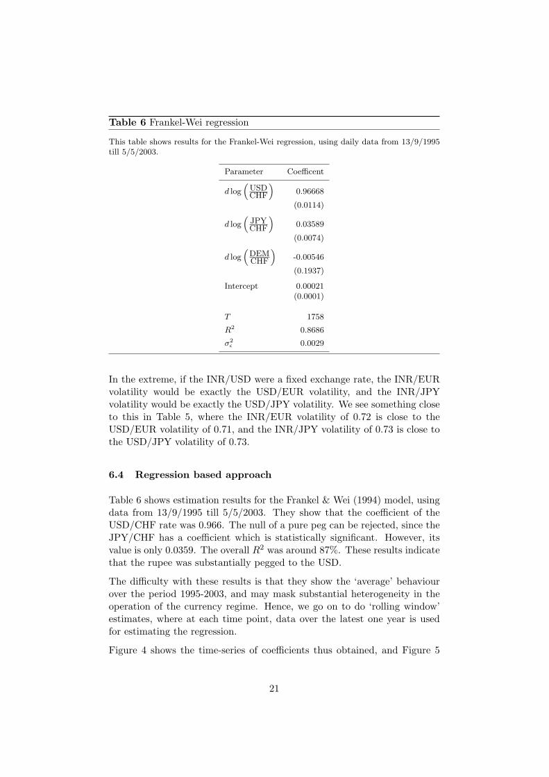
Table 6 Frankel-Wei regression

This table shows results for the Frankel-Wei regression, using daily data from 13/9/1995till 5/5/2003.

Parameter Coefficent

d log(

USDCHF

)0.96668

(0.0114)

d log(

JPYCHF

)0.03589

(0.0074)

d log(

DEMCHF

)-0.00546

(0.1937)

Intercept 0.00021(0.0001)

T 1758

R2 0.8686

σ2ε 0.0029

In the extreme, if the INR/USD were a fixed exchange rate, the INR/EURvolatility would be exactly the USD/EUR volatility, and the INR/JPYvolatility would be exactly the USD/JPY volatility. We see something closeto this in Table 5, where the INR/EUR volatility of 0.72 is close to theUSD/EUR volatility of 0.71, and the INR/JPY volatility of 0.73 is close tothe USD/JPY volatility of 0.73.

6.4 Regression based approach

Table 6 shows estimation results for the Frankel & Wei (1994) model, usingdata from 13/9/1995 till 5/5/2003. They show that the coefficient of theUSD/CHF rate was 0.966. The null of a pure peg can be rejected, since theJPY/CHF has a coefficient which is statistically significant. However, itsvalue is only 0.0359. The overall R2 was around 87%. These results indicatethat the rupee was substantially pegged to the USD.

The difficulty with these results is that they show the ‘average’ behaviourover the period 1995-2003, and may mask substantial heterogeneity in theoperation of the currency regime. Hence, we go on to do ‘rolling window’estimates, where at each time point, data over the latest one year is usedfor estimating the regression.

Figure 4 shows the time-series of coefficients thus obtained, and Figure 5

21

Figure 4 Rolling window Frankel-Wei regressions (coefficients)

0

0.2

0.4

0.6

0.8

1

1.2

Jan 95 Jan 96 Jan 97 Jan 98 Jan 99 Jan 00 Jan 01 Jan 02 Jan 03 Jan 04

Coe

ffici

ent i

n Fr

anke

l-Wei

regr

essi

on

USD/CHFJPY/CHF

DEM/CHF

Figure 5 Rolling window Frankel-Wei regressions (R2)

0.4

0.5

0.6

0.7

0.8

0.9

1

Jan 95 Jan 96 Jan 97 Jan 98 Jan 99 Jan 00 Jan 01 Jan 02 Jan 03 Jan 04

R2

of F

rank

el-W

ei re

gres

sion

22

Table 7 Prob values of the Box-Ljung Q statistic

USD EUR JPY

INR 0.0519 0.3050 0.3358USD 0.3265 0.1349EUR 0.2047

shows the time-series of the regression R2. We see that the coefficient of theUSD/CHF was near 1 through the entire period, barring a few periods wherethis coefficient slipped slightly (and other coefficients were higher). From1999 onwards, there appears to be a stable regime where the relationship isprimarily that with the USD. The time-series of the R2 vividly highlights thebrief period with greater currency flexibility, which is also seen in the time-series of λt, in 1998. After that, the R2 has been mostly near 1, suggestingthat pegging to the USD was the dominant factor in currency policy.

6.5 Market efficiency

We now turn to measurement of the extent to which the currency pairsunder estimation exhibit deviations from the random walk.

Table 7 shows prob values for the Box-Ljung portmanteu Q statistic, com-puted on the first 40 lags of the returns time-series. This is a simple measureof the extent to which the currency series violates the random walk. For thethree cross-currency pairs between the USD, EUR and JPY, we see probvalues of 0.32, 0.13 and 0.20, which suggest that for all the three cross-currency pairs, we cannot reject the null of a random walk at a 90% level ofsignificance.

Under the null of a managed INR/USD rate, we expected to find violationsof the random walk for the INR/USD. We find a prob value of 0.0519; thenull of a random walk would be rejected at a 94.2% level.

We argued that if the INR/USD is the subject of exchange rate policy, thenthe INR/USD series should suffer from rejections of the random walk, butother exchange rates of the INR should be unblemished. This is borne outin Table 7, where the Q statistic for the INR/EUR works out to 0.31 andthe Q statistic for the INR/JPY works out to 0.33. The violations of marketefficiency are limited to the INR/USD.

Figure 7 shows variance ratios for various lag lengths for three INR exchangerates, and Figure 6 shows variance ratios for the three currency pairs betweenthe USD, EUR and JPY. All six graphs here are superposed with criticalvalues for rejection at a 95% and 99% level of significance.

23

Figure 6 Variance ratio statistics for non-INR exchange rates

-1

-0.5

0

0.5

1

1.5

2

2.5

3

0 50 100 150 200 250

VR

(q)

Days

Variance Ratio (USDEURO)

Variance Ratio95% Bound99% Bound

-1

-0.5

0

0.5

1

1.5

2

2.5

3

0 50 100 150 200 250

VR

(q)

Days

Variance Ratio (EUROYEN)

Variance Ratio95% Bound99% Bound

-1

-0.5

0

0.5

1

1.5

2

2.5

3

0 50 100 150 200 250

VR

(q)

Days

Variance Ratio (USDYEN)

Variance Ratio95% Bound99% Bound

24

Figure 7 Variance ratio statistics for INR exchange rates

-1

-0.5

0

0.5

1

1.5

2

2.5

3

0 50 100 150 200 250

VR

(q)

Days

Variance Ratio (INRUSD)

Variance Ratio95% Bound99% Bound

-1

-0.5

0

0.5

1

1.5

2

2.5

3

0 50 100 150 200 250

VR

(q)

Days

Variance Ratio (INRYEN)

Variance Ratio95% Bound99% Bound

-1

-0.5

0

0.5

1

1.5

2

2.5

3

0 50 100 150 200 250

VR

(q)

Days

Variance Ratio (INREURO)

Variance Ratio95% Bound99% Bound

25

Table 8 Spectral tests of white noise for the INR/USD, from Wickham(2002)

Anderson-Darling Cramer - von Mises Kolmogorov- Kuiper SampleStatistic Statistic Smirnov Statistic Statistic Size

3-1-96 – 8-10-96 7.0321∗ 1.3910∗ 1.9836∗ 2.0607∗ 2009-10-96 – 3-11-97 13.6069∗ 209944∗ 2..6933∗ 2.8667∗ 2794-11-97 – 24-8-98 0.2750 0.0463 0.5140 0.7992 21025-8-98 – 29-12-00 9.0547∗ 1.8884∗ 2.4596∗ 2.5558∗ 614

Note: Values marked with a superscript ‘*’ are rejections at a 95% level.

Figure 6 is useful in illustrating how in a floating exchange rate regime,the price is a random walk, and all the variance ratio statistics come outto be roughly 1 at all lag lengths. This figure is a striking example of theeffectiveness of speculative markets at producing market efficiency.

Figure 7 shows the three currency pairs involving the INR. While the vari-ance ratios for the INR/USD do not generate rejection at the 95% levelof significance, they come close to that, and are strikingly different fromthe random walk character that is found in all the other variance ratios.This is consistent with the idea that the INR/USD rate does not enjoy theinformational efficiency of a price produced on a speculative market.

Such symptoms are not unique to India. Wickham (2002) finds that in aset of 16 developing countries which claim to have flexible exchange rates,7 exhibit discontinuities / regime shifts. Of the remaining 9, he finds threecountries where the daily returns process is not white noise, leaving onlysix out of sixteen developing countries where the claim of flexible exchangerates is not denied by empirical tests of white noise.

His evidence on India is consistent with our arguments above, and offersadditional insights. As shown in Table 8, he finds that for a brief periodfrom 4 November 1997 to 24 August 1998, the null of white noise cannot berejected, but over other periods, it can. These dates are tantalisingly relatedto the brief episode with a large value for λt that we find in Figure 3. Thismay suggest that in late 1997 and early 1998, India briefly experimentedwith greater exchange rate flexibility.

6.6 Is the REER or the NEER being targeted?

As argued above, if RBI were targeting the REER, then the REER shouldbe stable. The evidence seems to deny this. Table 9 compares the volatili-ties of five monthly time-series: two neer series, two reer series, and thenominal INR/USD exchange rate over the period April 1993 to December2002. The nominal INR/USD exchange rate has the lowest volatility of

26

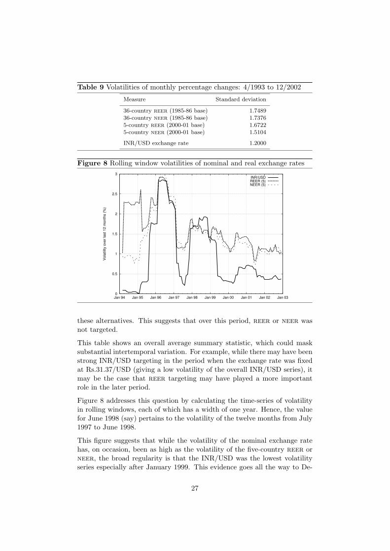
Table 9 Volatilities of monthly percentage changes: 4/1993 to 12/2002

Measure Standard deviation

36-country reer (1985-86 base) 1.748936-country neer (1985-86 base) 1.73765-country reer (2000-01 base) 1.67225-country neer (2000-01 base) 1.5104

INR/USD exchange rate 1.2000

Figure 8 Rolling window volatilities of nominal and real exchange rates

0

0.5

1

1.5

2

2.5

3

Jan 94 Jan 95 Jan 96 Jan 97 Jan 98 Jan 99 Jan 00 Jan 01 Jan 02 Jan 03

Vol

atili

ty o

ver l

ast 1

2 m

onth

s (%

)

INR/USDREER (5)NEER (5)

these alternatives. This suggests that over this period, reer or neer wasnot targeted.

This table shows an overall average summary statistic, which could masksubstantial intertemporal variation. For example, while there may have beenstrong INR/USD targeting in the period when the exchange rate was fixedat Rs.31.37/USD (giving a low volatility of the overall INR/USD series), itmay be the case that reer targeting may have played a more importantrole in the later period.

Figure 8 addresses this question by calculating the time-series of volatilityin rolling windows, each of which has a width of one year. Hence, the valuefor June 1998 (say) pertains to the volatility of the twelve months from July1997 to June 1998.

This figure suggests that while the volatility of the nominal exchange ratehas, on occasion, been as high as the volatility of the five-country reer orneer, the broad regularity is that the INR/USD was the lowest volatilityseries especially after January 1999. This evidence goes all the way to De-

27

cember 2002, and hence reflects the contemporary currency regime. Thisappears to be more consistent with the hypothesis that the currency regimewas focused on the nominal exchange rate. However, these estimates userolling window volatilities for one year. They could fail to pick up reertargetting for over longer time horizons.

7 Conclusion

In this paper, we had set out to obtain some insights into India’s experiencewith the currency regime, and the accumulation of reserves in recent years.Did the reserves growth in India, and particularly that observed in the lastone to two years, take place as a consequence of a policy that targeted acertain minimum level of ‘reserves as insurance’, or did the reserves growthtake place as a passive side effect of maintaining the currency regime?

These questions are inextricably intertwined with the question of character-ising India’s currency regime. This is related to the puzzle of interpretingthe phrase ‘market determined exchange rate’ that is used by RBI. Theexisting currency regime is not based on a transparent set of publicly dis-closed rules. The official stance of the RBI about the nature of the currencyregime should be approached with caution, given the extensive internationalevidence that central banks do not do what they say. Hence an analysis ofthe data is required in understanding the underlying currency regime.

In this paper, we repeatedly resolve questions about the goals of policy byfocusing upon volatility. In a system where x and y are related variables,and if x is targeted, then x will experience low volatility and y will expe-rience enhanced volatility if it is either the instrument used by the policymaker, or a side effect of policy measures focused on x. This approach al-lows us to disentangle the true goals of policy from the ‘side effects’ andinstrumentalities of attaining these goals.

We compare India’s reserves holdings against a variety of metrics that havebeen proposed in the literature. It appears that by March 2002, India hadadequate reserves going by all these metrics. In this case, the addition of$20 billion after this point does not support the proposition that the RBIwas motivated by reserves as insurance.

The currency market betrays strong symptoms of a highly managed INR/USDexchange rate, as has been pointed out by two prominent papers in 2002(Reinhart & Rogoff 2002, Calvo & Reinhart 2002). We argue that if a nullhypothesis “the INR/USD is the central focus of exchange rate manage-ment” is maintained, this leads to predictions which are substantiated bythe evidence. The regression framework of Frankel & Wei (1994) is alsoconsistent with the hypothesis of a nominal peg to the USD. This suggests

28

that India has primarily had a nominal exchange rate policy in recent years,and that reserves accretion has been the side effect of this policy. We ae alsoable to reject the hypothesis that in the over a one year horizon the RBItargets the reer.

It appears that the phrase ‘market determined exchange rate’ should beusefully interpreted as saying that the exchange rate is shaped on a market,and not administratively determined, as was the case in preceding decades.However, it should not be interpreted as meaning that the exchange rate isdetermined out of the equilibrium obtained from a large mass of economicagents on the currency market. RBI appears to be an active trader on themarket, using the large size of its transactions to manipulate the marketprice.

As the literature suggests, India has been in a homogeneous regime of lowexchange rate flexibility from 1979 onwards. In the older period, the highlyrepressed external sector may have made it easier to achieve goals of cur-rency policy without repercussions for the domestic economy. However, thesteady liberalisation of the external sector implies that other elements of pol-icy, particularly reserves and monetary policy, now have to undergo greaterstress in order to achieve traditional goals of exchange rate policy.

The arguments of this paper are useful in understanding Indian macroeco-nomics and macro policy today. The loss of monetary policy independencethat accompanies an open capital account and a flexible exchange rate cre-ate new policy dilemmas. When exchange rate adjustment is muted, othervariables in the economy have to adjust in response to shocks. Moreover,currency regimes with exchange rate targeting are vulnerable to speculativeattacks. The failures of market efficiency that this paper documents suggeststhat there are opportunities for profitable speculative trading strategies. Themonetary impact of the current exchange rate regime and questions aboutspeculative activity are topics for further research.

29

References

Aizenman, J. & Marion, N. (2002), The high demand for international reserves inthe Far East: What’s going on?, Technical report, UC, Santa Cruz and Dart-mouth College.

Baig, T. (2001), Characterising exchange rate regimes in post-crisis East Asia,Technical Report WP/01/152, IMF.

Bayoumi, T. & Eichengreen, B. (1998), ‘Exchange rate volatility and intervention:Implications of the theory of optimum currency areas’, Journal of InternationalEconomics 45, 191–209.

Calvo, G. A. & Reinhart, C. M. (2002), ‘Fear of floating’, Quarterly Journal ofEconomics CXVII(2), 379–408.

Cochrane, J. (1988), ‘How Big is the Random Walk in GDP?’, Journal of PoliticalEconomy 96, 893–920.

Frankel, J. & Wei, S.-J. (1994), Yen bloc or dollar bloc? Exchange rate policies ofthe East Asian countries, in T. Ito & A. Krueger, eds, ‘Macroeconomic linkage:Savings, exchange rates and capital flows’, University of Chicago Press.

Ghosh, S. K. (2002), ‘RBI intervention in the forex market’, Economic and PoliticalWeekly v(n), 2333–2348.

Glick, R. & Wihlborg, C. (1997), Exchange rate regimes and international trade,in P. Kenen & B. Cohen, eds, ‘International trade and finance: New frontiers forresearch’, Cambridge University Press.

Hawkins, J. & Turner, P. (2000), Managing foreign debt and liquidity risks inemerging economies: An overview, Policy Papers 8, BIS.

Jalan, B. (1999), ‘International financial architecture: Developing countries’ per-spective’, RBI Bulletin .

Jalan, B. (2002), India’s economy in the new millennium: Selected essays, UBSPublishers and distributors.

Kapur, D. & Patel, U. R. (2003), ‘Large foreign currency reserves: Insurance fordomestic weaknesses and external uncertainties?’, Economic and Political WeeklyXXXVIII(11), 1047–1053.

Kim, M. J., Nelson, C. R. & Startz, R. (1991), ‘Mean Reversion in Stock Prices?A Reappraisal of the Empirical Evidence’, Review of Economic Studies 58, 515–528.

Lo, A. & MacKinlay, C. (1988), ‘Stock Market Prices do not follow Random Walks:Evidence from a Simple Specification Test’, Review of Financial Studies 1, 41–66.

Obstfeld, M. & Rogoff, K. S. (1995), ‘The mirage of fixed exchange rates’, Journalof Economic Perspectives 9(4), 73–96.

Patnaik, I. & Pauly, P. (2001), ‘The Indian foreign exchange market and the equi-librium real exchange rate of the rupee’, Global Business Review 2(2).

30

Patnaik, T. & Thomas, S. (2003), Variance-ratio tests and high-frequency data: Astudy of liquidity and mean reversion in the Indian equity markets, Technicalreport, IGIDR, Mumbai.

Ranade, A. & Kapur, G. (2003), ‘Appreciating rupee: Changing paradigm?’, Eco-nomic and Political Weekly XXXVIII(8), 769–775.

Rangarajan, C. (1993), Report of the high level committee on balance of payments,Committee report, Reserve Bank of India.

RBI (2002), Annual report 2001-02, Technical report, Reserve Bank of India.

Reinhart, C. M. & Rogoff, K. S. (2002), The modern history of exchange ratearrangements: A reinterpretation, Technical Report 8963, NBER.

Tarapore, S. (1997), Report of the committee on capital account liberalisation,Committee report, Reserve Bank of India.

Wickham, P. (2002), Do “flexible” exchange rates of developing countries be-have like floating exchange rates of industrialised countries?, Technical ReportWP/02/82, IMF.

31