Incorporating Qualitative Information into Quantitative Estimation viaSequentially Constrained Hamiltonian Monte Carlo Sampling

Daqing Yi, Shushman Choudhury and Siddhartha Srinivasa

Abstract—In human-robot collaborative tasks, incorporatingqualitative information provided by humans can greatly en-hance the robustness and efficacy of robot state estimation.We introduce an algorithmic framework to model qualitativeinformation as quantitative constraints on and between states.Our approach, named Sequentially Constrained HamiltonianMonte Carlo, integrates Hamiltonian dynamics into Sequen-tially Constrained Monte Carlo sampling. We are able to gen-erate samples that satisfy arbitrarily complex, non-smooth anddiscontinuous constraints, which in turn allows us to support awide range of qualitative information. We evaluate our approachfor constrained sampling qualitatively and quantitatively withseveral classes of constraints. SCHMC significantly outperformsthe Metropolis-Hastings algorithm (a standard Markov ChainMonte Carlo (MCMC) method) and the Hamiltonian MonteCarlo (HMC) method, in terms of both the accuracy ofthe sampling (for satisfying constraints) and the quality ofapproximation. Compared to Sequentially Constrained MonteCarlo (SCMC), which supports similar kinds of constraints,our SCHMC approach has faster convergence rates and lowerparameter sensitivity.

I. INTRODUCTION

We consider the problem of leveraging numerous forms ofinformation for state estimation applications. A widely stud-ied instance of this is the sensor fusion problem [10], whichmerges information from multiple sensors and sources [17]for estimating hidden states. We are interested in a related butdifferent setting - incorporating information from humans.

In a collaborative human-robot team, both the human(s)and the robot(s) receive observations from the shared en-vironment. There are several potential benefits to this, de-scribed in Section II. The sensing capabilities of the humancomplements that of a robot [12], often overcoming many ofthe robot’s perceptual limitations [13] The human-suppliedqualitative information helps enhance the robustness of esti-mation and reduce the uncertainty. For instance, informationfrom experienced human rescuers has been used to moresuccessfully predict the location of a target [1]. Furthermore,the human can provide knowledge about the physical worldwhich facilitates corrections during state estimation [22].Humans can provide qualitative descriptions [4] or high-levelinstructions [26] to help a robot with task execution.

Qualitative information from the human can be providedin several forms:

• A general description of a state that constrains the valuesof the state.

All authors are with Robotics Institute, CarnegieMellon University. daqingy@andrew.cmu.edu,shushmac@andrew.cmu.edu, siddh@cs.cmu.edu

(a) A map sketch [1] (b) No collision [22] (c) Spatial relation [4]

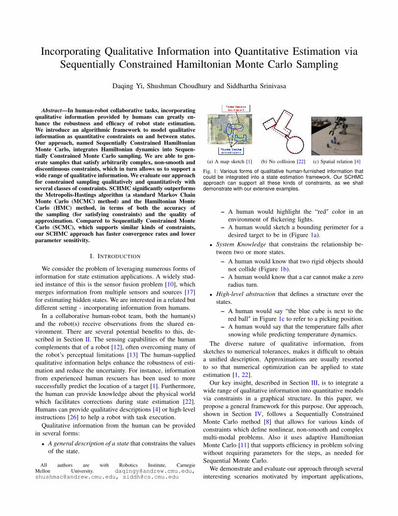
Fig. 1: Various forms of qualitative human-furnished information thatcould be integrated into a state estimation framework. Our SCHMCapproach can support all these kinds of constraints, as we shalldemonstrate with our extensive examples.

– A human would highlight the “red" color in anenvironment of flickering lights.

– A human would sketch a bounding perimeter for adesired target to be in (Figure 1a).

• System Knowledge that constrains the relationship be-tween two or more states.

– A human would know that two rigid objects shouldnot collide (Figure 1b).

– A human would know that a car cannot make a zeroradius turn.

• High-level abstraction that defines a structure over thestates.

– A human would say “the blue cube is next to thered ball" in Figure 1c to refer to a picking position.

– A human would say that the temperature falls aftersnowing while predicting temperature dynamics.

The diverse nature of qualitative information, fromsketches to numerical tolerances, makes it difficult to obtaina unified description. Approximations are usually resortedto so that numerical optimization can be applied to stateestimation [1, 22].

Our key insight, described in Section III, is to integrate awide range of qualitative information into quantitative modelsvia constraints in a graphical structure. In this paper, wepropose a general framework for this purpose. Our approach,shown in Section IV, follows a Sequentially ConstrainedMonte Carlo method [8] that allows for various kinds ofconstraints which define nonlinear, non-smooth and complexmulti-modal problems. Also it uses adaptive HamiltonianMonte Carlo [11] that supports efficiency in problem solvingwithout requiring parameters for the steps, as needed forSequential Monte Carlo.

We demonstrate and evaluate our approach through severalinteresting scenarios motivated by important applications,

outlined in Section V. Since our focus is on the mathematicaldetails and implementation of the underlying algorithm, weuse simulated examples of constrained sampling, filtering,and static state estimation that are easy to visualize. Thisalso helps us highlight the versatility of our approach bydemonstrating support for a number of different kinds ofconstraints.

II. RELATED WORK

In a fusion framework, information is typically modeled asa random variable, so a common way of presenting humaninformation is “soft data”, using a probability distribution [2].In a human-robot team, a robot can convert a qualitativedescription of the environment into a distribution to support asearch task [16, 24]. Qualitative spatial relations from humanshas been modeled into map generation for navigation [18].A hand-sketched path and map has been used as a prior fora robot’s simultaneous mapping and navigation [21].

Another approach of modeling qualitative information isas a “hard constraint". For planning a shared task, a humancan generate a path shape as a topological constraint for therobot’s planning and execution [25, 26]. Moreover, a lot ofphysics-based knowledge can be modeled as constraints instate estimation. The collision-free constraint for rigid bodiesis used in correcting state estimation of object positions [22].Hard constraints enforce the relationship between states,which reduces the uncertainty of state estimation [23], thoughit does increase the difficulty of problem solving.

In solving a constrained nonlinear optimization problem,sequential quadratic programming is a popular tool [22] thatdecomposes a problem into a sequence of subproblems andsolves them iteratively. It requires the objective and theconstraints to be twice differentiable, which greatly limits thesupport for constraints derived from qualitative information.For example, a hand sketch in Figure 1a can be difficultto convert into a mathematical description in a probabilisticinference framework. The solution is determined by the initialguess, and only local optimality is guaranteed.

One way to achieve global optimality is through MonteCarlo simulation. Markov Chain Monte Carlo [5](MCMC)is a computational technique that derives a set of samples toapproximate a probability distribution by modeling a MarkovChain random walk. It recovers more information about adistribution than only estimating an optimal solution [5].Sequential Monte Carlo [6] introduces a set of samples thatform parallel Markov Chains from a sequence of bridgingdistributions for complex multimodal distributions, whichapplies to high dimensional spaces [20] and complex con-straints [9]. Various transition kernels can be used in Sequen-tial Monte Carlo [20]. Hamiltonian dynamics [19] have beenintroduced as a more efficient alternative to the random walkMCMC kernel for moving samples around. Therefore, weuse an adaptive Hamiltonian Monte Carlo [11](HMC) kernelin a Sequentially Constrained Monte Carlo [8] framework forour overall approach.

III. PROBLEM STATEMENT

Assume we have a set of observations O = {o1, · · · , oN}that is associated with a set of states X = {x1, · · · , xK}.In a problem that considers only quantitative information,state estimation can usually be defined as a MAP (MaximumAposteriori Probability) problem, which is

X̂∗ = arg maxX

P (X | O). (1)

We propose two types of qualitative information to modelhuman information - feature and relation.• Feature informs a property of a state. Let f(x) ≤ 0

when the constraint is satisfied.• Relation informs a conditional relationship between

two states. Let f(x2 | x1) ≤ 0 when the constraintis satisfied. Often, f(x2 | x1) and f(x1 | x2) areboth equivalent to a mutual relation f(x1, x2), whichis satisfied when f(x1, x2) ≤ 0.

Some examples of qualitative information are given below.• The color is red. Assume the color is represented in HSV

space and the H value h ∈ [0, 180]. The information“red color" indicates a feature that constrains the valueof state h to be in [0, 10] ∪ [160, 180].

• The object is on the left hand side. Assuming the x-coordinate on the left hand side is all negative, thisdefines a feature that constrains the object location asx ≤ 0.

• Ball one and ball two are rigid. Let s1 be the estimatedcenter of ball one with radius r1. Let s2 be the centerof a ball with radius r2. If the two balls cannot collide,we have |s1 − s2| ≥ r1 + r2 as a constraint.

• The point is inside a circle. Assume the circle is a unitcircle centered at the origin. This information impliesthat given y, x should satisfy x−

√1− y2 ≤ 0∧−x−√

1− y2 ≤ 0. Similarly, given x, y should satisfy y −√1− x2 ≤ 0 ∧ −y −

√1− x2 ≤ 0.

• The object is a square. Let s1, s2, s3, s4 be the estimatedcorners of a square on a plane and r be the estimatededge length of the square. By prior geometric knowl-edge, we have |s1−s2| = r, |s2−s3| = r, |s3−s4| = rand |s4 − s1| = r as constraints.

• A human sketches a region. A human sketches a regionon a map that indicates where a target is, as in Figure1a. Let s be the estimated position of the target and Rbe a human-sketched region. This information implies afeature that requires s ∈ R.

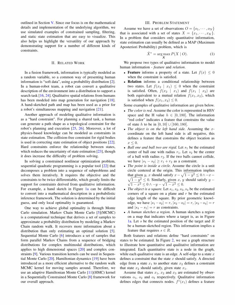
Both features and relations define “hard constraints" onstates to be estimated. In Figure 2, we use a graph structureto illustrate how quantitative and qualitative information areintegrated. Each quantitative state is a node in the graph,while each qualitative state is an edge. A self-edge to a state xdefines a constraint that the state x should satisfy. A directededge from a state x1 to another state x2 defines a constraintthat state x2 should satisfy, given state x1.

Assume that states x1, x2 and x3 are estimated by obser-vations o1, o2 and o3 respectively. Qualitative informationdefines edges that connects nodes. f1(x1) defines a feature

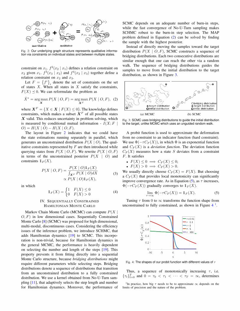
Fig. 2: Our underlying graph structure represents qualitative informa-tion via constraints on individual states and between multiple states.

constraint on x1. f2(x2 | x1) defines a relation constraint onx2 given x1. f3(x3 | x2) and f4(x2 | x3) together define arelation constraint on x2 and x3.

Let F ={f i}i

denote the set of constraints on the setof states X . When all states in X satisfy the constraints,F (X) � 0. We can reformulate the problem as

X̂∗ = arg maxX

P (X | O,F ) = arg maxXF

P (X | O,F ), (2)

where XF = {X ∈X | F (X) ≤ 0}. The knowledge definesconstraints, which makes a subset XF of all possible statesX valid. This reduces uncertainty in problem solving, whichis measured by conditional mutual information - I(X;F |O) = H(X | O)−H(X | O,F ).

The layout in Figure 2 indicates that we could havethe state estimations running separately in parallel, whichgenerates an unconstrained distribution P (X | O). The qual-itative constraints represented by F are then introduced whilequerying states from P (X | O,F ). We rewrite P (X | O,F )in terms of the unconstrained posterior P (X | O) andconstraints 1F (X).

P (X | O,F ) =P (X | O)1F (X)∫XF P (X | O)dX

∝ P (X | O)1F (X),

(3)

in which

1F (X) =

{1 F (X) ≤ 00 F (X) > 0

(4)

IV. SEQUENTIALLY CONSTRAINEDHAMILTONIAN MONTE CARLO

Markov Chain Monte Carlo (MCMC) can compute P (X |O,F ) in low dimensional cases. Sequentially ConstrainedMonte Carlo [8] (SCMC) was proposed for high dimensional,multi-modal, discontinuous cases. Considering the efficiencyissues of the inference problem, we introduce SCHMC, thatadds Hamiltonian dynamics [19] to SCMC. This incorpo-ration is non-trivial, because for Hamiltonian dynamics inthe general MCMC, the performance is heavily dependenton selecting the number and length of the steps [19]. Thisproperty prevents it from fitting directly into a sequentialMonte Carlo structure, because bridging distributions mightrequire different parameters while selecting steps. Bridgingdistributions denote a sequence of distributions that transitionfrom an unconstrained distribution to a fully constraineddistribution. We use a kernel obtained from No-U-Turn sam-pling [11], that adaptively selects the step length and numberfor Hamiltonian dynamics. Moreover, the performance of

SCMC depends on an adequate number of burn-in steps,while the fast convergence of No-U-Turn sampling makesSCHMC robust to the burn-in step selection. The MAPproblem defined in Equation (2) can be solved by findingthe sample with the highest posterior.

Instead of directly moving the samples toward the targetdistribution P (X | O,F ), SCMC constructs a sequence ofbridging distributions. Each two consecutive distributions aresimilar enough that one can reach the other via a randomwalk. The sequence of bridging distributions guides thesamples to move from the initial distribution to the targetdistribution, as shown in Figure 3.

(a) MCMC (b) SCMC

Fig. 3: SCMC uses bridging distributions to guide the initial distributionto the target, unlike MCMC which uses an unguided random walk.

A probit function is used to approximate the deformationfrom no constraint to an indicator function (hard constraint).We use Φ(−τCF (X)), in which Φ is an exponential functionand CF (X) is a deviation function. The deviation functionCF (X) measures how a state S deviates from a constraintF . It satisfies• F (X) ≤ 0 =⇒ CF (X) ≤ 0;• F (X) > 0 =⇒ CF (X) > 0.

We usually directly choose CF (X) = F (X). But choosinga CF (X) that provides local monotonicity can significantlyimprove convergence rate. As in Equation (5), as τ increases,Φ(−τCF (X)) gradually converges to 1F (X).

limτ→∞

Φ(−τCF (X)) = 1F (X). (5)

Tuning τ from 0 to ∞ transforms the function shape fromunconstrained to fully constrained, as shown in Figure 4 1.

Fig. 4: The shapes of our probit function with different values of τ

Thus, a sequence of monotonically increasing τ , i.e.{τt}Tt=0 and 0 = τ0 < τ1 < · · · < τT = ∞, determines

1In practice, how big τ needs to be to approximate ∞ depends on thelimits of precision and the nature of the problem.

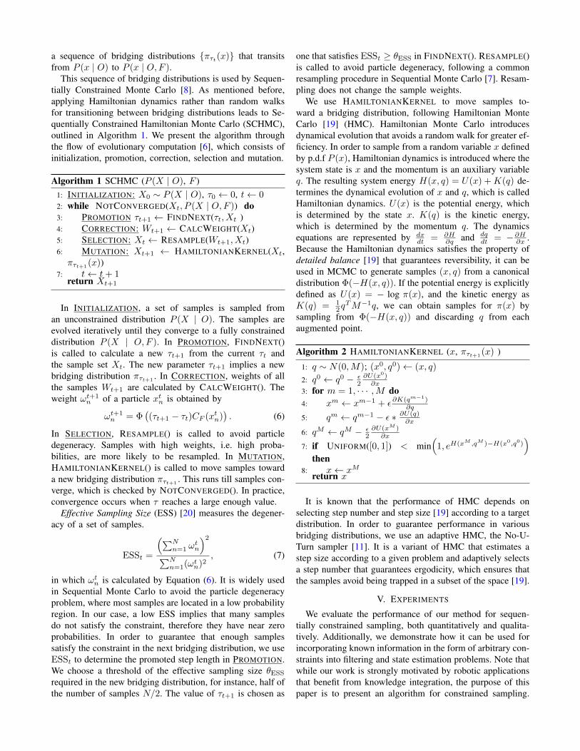
a sequence of bridging distributions {πτt(x)} that transitsfrom P (x | O) to P (x | O,F ).

This sequence of bridging distributions is used by Sequen-tially Constrained Monte Carlo [8]. As mentioned before,applying Hamiltonian dynamics rather than random walksfor transitioning between bridging distributions leads to Se-quentially Constrained Hamiltonian Monte Carlo (SCHMC),outlined in Algorithm 1. We present the algorithm throughthe flow of evolutionary computation [6], which consists ofinitialization, promotion, correction, selection and mutation.

Algorithm 1 SCHMC (P (X | O), F )1: INITIALIZATION: X0 ∼ P (X | O), τ0 ← 0, t← 02: while NOTCONVERGED(Xt, P (X | O,F )) do3: PROMOTION τt+1 ← FINDNEXT(τt, Xt )4: CORRECTION: Wt+1 ← CALCWEIGHT(Xt)5: SELECTION: Xt ← RESAMPLE(Wt+1, Xt)6: MUTATION: Xt+1 ← HAMILTONIANKERNEL(Xt,πτt+1(x))

7: t← t+ 1return Xt+1

In INITIALIZATION, a set of samples is sampled froman unconstrained distribution P (X | O). The samples areevolved iteratively until they converge to a fully constraineddistribution P (X | O,F ). In PROMOTION, FINDNEXT()is called to calculate a new τt+1 from the current τt andthe sample set Xt. The new parameter τt+1 implies a newbridging distribution πτt+1

. In CORRECTION, weights of allthe samples Wt+1 are calculated by CALCWEIGHT(). Theweight ωt+1

n of a particle xtn is obtained by

ωt+1n = Φ

((τt+1 − τt)CF (xtn)

). (6)

In SELECTION, RESAMPLE() is called to avoid particledegeneracy. Samples with high weights, i.e. high proba-bilities, are more likely to be resampled. In MUTATION,HAMILTONIANKERNEL() is called to move samples towarda new bridging distribution πτt+1 . This runs till samples con-verge, which is checked by NOTCONVERGED(). In practice,convergence occurs when τ reaches a large enough value.

Effective Sampling Size (ESS) [20] measures the degener-acy of a set of samples.

ESSt =

(∑Nn=1 ω

tn

)2∑Nn=1(ωtn)2

, (7)

in which ωtn is calculated by Equation (6). It is widely usedin Sequential Monte Carlo to avoid the particle degeneracyproblem, where most samples are located in a low probabilityregion. In our case, a low ESS implies that many samplesdo not satisfy the constraint, therefore they have near zeroprobabilities. In order to guarantee that enough samplessatisfy the constraint in the next bridging distribution, we useESSt to determine the promoted step length in PROMOTION.We choose a threshold of the effective sampling size θESS

required in the new bridging distribution, for instance, half ofthe number of samples N/2. The value of τt+1 is chosen as

one that satisfies ESSt ≥ θESS in FINDNEXT(). RESAMPLE()is called to avoid particle degeneracy, following a commonresampling procedure in Sequential Monte Carlo [7]. Resam-pling does not change the sample weights.

We use HAMILTONIANKERNEL to move samples to-ward a bridging distribution, following Hamiltonian MonteCarlo [19] (HMC). Hamiltonian Monte Carlo introducesdynamical evolution that avoids a random walk for greater ef-ficiency. In order to sample from a random variable x definedby p.d.f P (x), Hamiltonian dynamics is introduced where thesystem state is x and the momentum is an auxiliary variableq. The resulting system energy H(x, q) = U(x) +K(q) de-termines the dynamical evolution of x and q, which is calledHamiltonian dynamics. U(x) is the potential energy, whichis determined by the state x. K(q) is the kinetic energy,which is determined by the momentum q. The dynamicsequations are represented by dx

dt = ∂H∂q and dq

dt = −∂H∂x .Because the Hamiltonian dynamics satisfies the property ofdetailed balance [19] that guarantees reversibility, it can beused in MCMC to generate samples (x, q) from a canonicaldistribution Φ(−H(x, q)). If the potential energy is explicitlydefined as U(x) = − log π(x), and the kinetic energy asK(q) = 1

2qTM−1q, we can obtain samples for π(x) by

sampling from Φ(−H(x, q)) and discarding q from eachaugmented point.

Algorithm 2 HAMILTONIANKERNEL (x, πτt+1(x) )

1: q ∼ N(0,M); (x0, q0)← (x, q)

2: q0 ← q0 − ε2∂U(x0)∂x

3: for m = 1, · · · ,M do4: xm ← xm−1 + ε∂K(qm−1)

∂q

5: qm ← qm−1 − ε ∗ ∂U(q)∂x

6: qM ← qM − ε2∂U(xM )∂x

7: if UNIFORM([0, 1]) < min(

1, eH(xM ,qM )−H(x0,q0))

then8: x← xM

return x

It is known that the performance of HMC depends onselecting step number and step size [19] according to a targetdistribution. In order to guarantee performance in variousbridging distributions, we use an adaptive HMC, the No-U-Turn sampler [11]. It is a variant of HMC that estimates astep size according to a given problem and adaptively selectsa step number that guarantees ergodicity, which ensures thatthe samples avoid being trapped in a subset of the space [19].

V. EXPERIMENTS

We evaluate the performance of our method for sequen-tially constrained sampling, both quantitatively and qualita-tively. Additionally, we demonstrate how it can be used forincorporating known information in the form of arbitrary con-straints into filtering and state estimation problems. Note thatwhile our work is strongly motivated by robotic applicationsthat benefit from knowledge integration, the purpose of thispaper is to present an algorithm for constrained sampling.

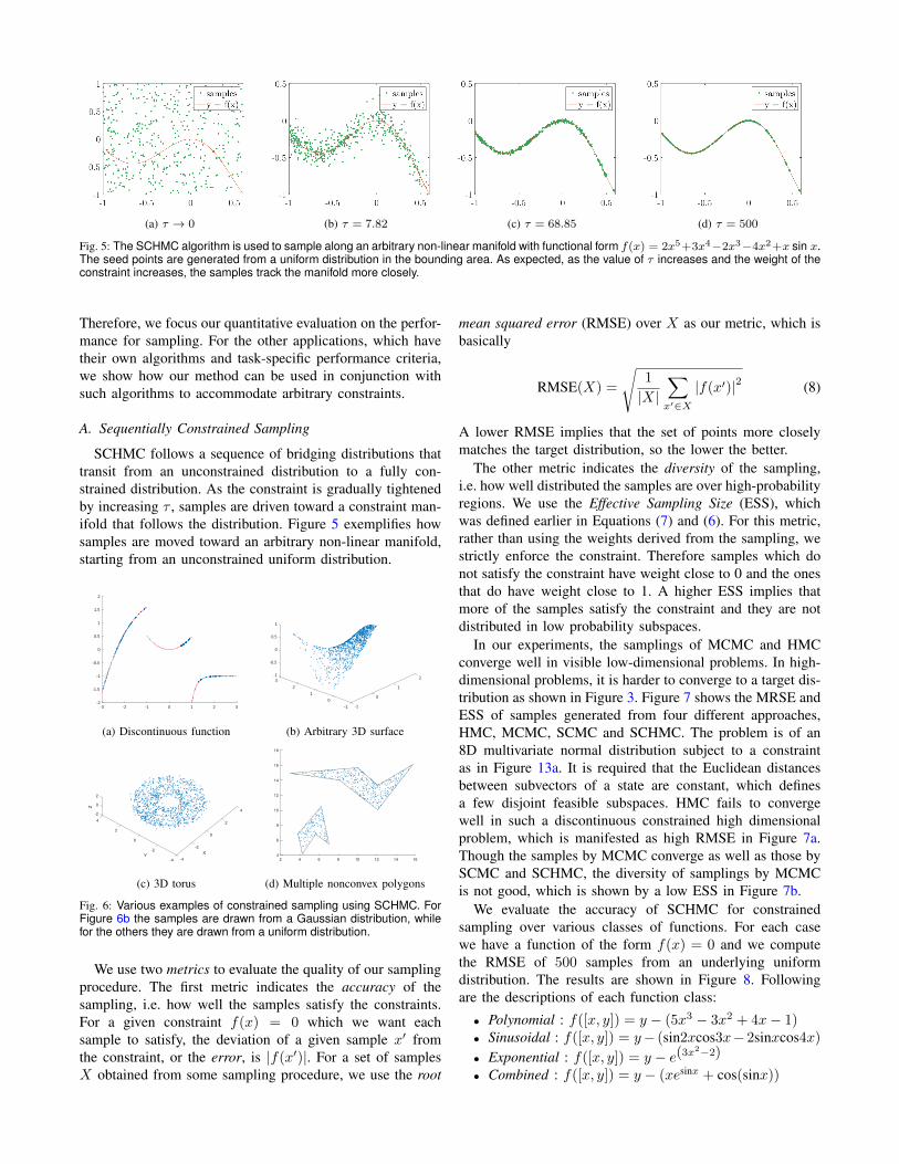
(a) τ → 0 (b) τ = 7.82 (c) τ = 68.85 (d) τ = 500

Fig. 5: The SCHMC algorithm is used to sample along an arbitrary non-linear manifold with functional form f(x) = 2x5+3x4−2x3−4x2+x sin x.The seed points are generated from a uniform distribution in the bounding area. As expected, as the value of τ increases and the weight of theconstraint increases, the samples track the manifold more closely.

Therefore, we focus our quantitative evaluation on the perfor-mance for sampling. For the other applications, which havetheir own algorithms and task-specific performance criteria,we show how our method can be used in conjunction withsuch algorithms to accommodate arbitrary constraints.

A. Sequentially Constrained Sampling

SCHMC follows a sequence of bridging distributions thattransit from an unconstrained distribution to a fully con-strained distribution. As the constraint is gradually tightenedby increasing τ , samples are driven toward a constraint man-ifold that follows the distribution. Figure 5 exemplifies howsamples are moved toward an arbitrary non-linear manifold,starting from an unconstrained uniform distribution.

-3 -2 -1 0 1 2 3-2

-1.5

-1

-0.5

0

0.5

1

1.5

2

(a) Discontinuous function

2-13

-0.5

2 1

0

10

0.5

0

-1-1

1

(b) Arbitrary 3D surface

4-24 2

2

X

0

Y

0-2

-2

-4-4

0Z

2

(c) 3D torus

2 4 6 8 10 12 14 164

6

8

10

12

14

16

18

(d) Multiple nonconvex polygons

Fig. 6: Various examples of constrained sampling using SCHMC. ForFigure 6b the samples are drawn from a Gaussian distribution, whilefor the others they are drawn from a uniform distribution.

We use two metrics to evaluate the quality of our samplingprocedure. The first metric indicates the accuracy of thesampling, i.e. how well the samples satisfy the constraints.For a given constraint f(x) = 0 which we want eachsample to satisfy, the deviation of a given sample x′ fromthe constraint, or the error, is |f(x′)|. For a set of samplesX obtained from some sampling procedure, we use the root

mean squared error (RMSE) over X as our metric, which isbasically

RMSE(X) =

√1

|X|∑x′∈X

|f(x′)|2 (8)

A lower RMSE implies that the set of points more closelymatches the target distribution, so the lower the better.

The other metric indicates the diversity of the sampling,i.e. how well distributed the samples are over high-probabilityregions. We use the Effective Sampling Size (ESS), whichwas defined earlier in Equations (7) and (6). For this metric,rather than using the weights derived from the sampling, westrictly enforce the constraint. Therefore samples which donot satisfy the constraint have weight close to 0 and the onesthat do have weight close to 1. A higher ESS implies thatmore of the samples satisfy the constraint and they are notdistributed in low probability subspaces.

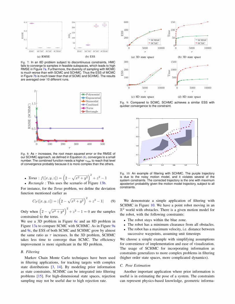
In our experiments, the samplings of MCMC and HMCconverge well in visible low-dimensional problems. In high-dimensional problems, it is harder to converge to a target dis-tribution as shown in Figure 3. Figure 7 shows the MRSE andESS of samples generated from four different approaches,HMC, MCMC, SCMC and SCHMC. The problem is of an8D multivariate normal distribution subject to a constraintas in Figure 13a. It is required that the Euclidean distancesbetween subvectors of a state are constant, which definesa few disjoint feasible subspaces. HMC fails to convergewell in such a discontinuous constrained high dimensionalproblem, which is manifested as high RMSE in Figure 7a.Though the samples by MCMC converge as well as those bySCMC and SCHMC, the diversity of samplings by MCMCis not good, which is shown by a low ESS in Figure 7b.

We evaluate the accuracy of SCHMC for constrainedsampling over various classes of functions. For each casewe have a function of the form f(x) = 0 and we computethe RMSE of 500 samples from an underlying uniformdistribution. The results are shown in Figure 8. Followingare the descriptions of each function class:

• Polynomial : f([x, y]) = y − (5x3 − 3x2 + 4x− 1)• Sinusoidal : f([x, y]) = y− (sin2xcos3x− 2sinxcos4x)

• Exponential : f([x, y]) = y − e(3x2−2)

• Combined : f([x, y]) = y − (xesinx + cos(sinx))

HMC MCMC SCMC SCHMC0

0.1

0.2

0.3RMSE

(a) RMSE

HMC MCMC SCMC SCHMC

0

50

100

150

200

250

ESSF

(b) ESS

Fig. 7: In an 8D problem subject to discontinuous constraints, HMCfails to converge to samples in feasible subspaces, which leads to highRMSE in Figure 7a. Furthermore, the diversity of sampling with MCMCis much worse than with SCMC and SCHMC. Thus the ESS of MCMCin Figure 7b is much lower than that of SCMC and SCHMC. The resultsare averaged over 10 different runs.

Fig. 8: As τ increases, the root mean squared error or the RMSE ofour SCHMC approach, as defined in Equation (8), converges to a smallnumber. The combined function needs a higher τmax to reach that levelof convergence probably because it is more complex than the others.

• Torus : f([x, y, z]) =(

2−√x2 + y2

)2+ z2 − 1

• Rectangle : This uses the scenario of Figure 13b.For instance, for the Torus problem, we define the deviationfunction mentioned earlier as

CF ([x, y, z]) = |(

2−√x2 + y2

)2+ z2 − 1| (9)

Only when(

2−√x2 + y2

)2+ z2 − 1 = 0 are the samples

constrained to the torus.We use a 3D problem in Figure 6c and an 8D problem inFigure 13a to compare SCMC with SCHMC. As in Figure 9aand 9c, the ESS of both SCMC and SCHMC grow by almostthe same ratio as τ increases. In the 3D problem, SCHMCtakes less time to converge than SCMC. The efficiencyimprovement is more significant in the 8D problem.

B. Filtering

Markov Chain Monte Carlo techniques have been usedin filtering applications, for tracking targets with complexstate distributions [3, 14]. By modeling prior informationas state constraints, SCHMC can be integrated into filteringproblems [15]. For high-dimensional state spaces, rejectionsampling may not be useful due to high rejection rate.

(a) 3D state space (b) 3D state space

(c) 8D state space (d) 8D state space

Fig. 9: Compared to SCMC, SCHMC achieves a similar ESS withquicker convergence to the constraint.

Fig. 10: An example of filtering with SCHMC. The purple trajectoryis due to the noisy motion model, and it violates several of thesystem constraints. The corrected trajectory is the one with maximumaposteriori probability given the motion model trajectory, subject to allconstraints.

We demonstrate a simple application of filtering withSCHMC in Figure 10. We have a point robot moving in anR2 world with obstacles. There is a given motion model forthe robot, with the following constraints:• The robot stays within the blue zone.• The robot has a minimum clearance from all obstacles.• The robot has a maximum velocity, i.e. distance between

successive waypoints, assuming unit timestepsWe choose a simple example with simplifying assumptionsfor convenience of implementation and ease of visualization.The usage of SCHMC for incorporating information asconstraints generalizes to more complex problems in filtering(higher order state spaces, more complicated dynamics).

C. Pose Estimation

Another important application where prior information isuseful is in estimating the pose of a system. The constraintscan represent physics-based knowledge, geometric informa-

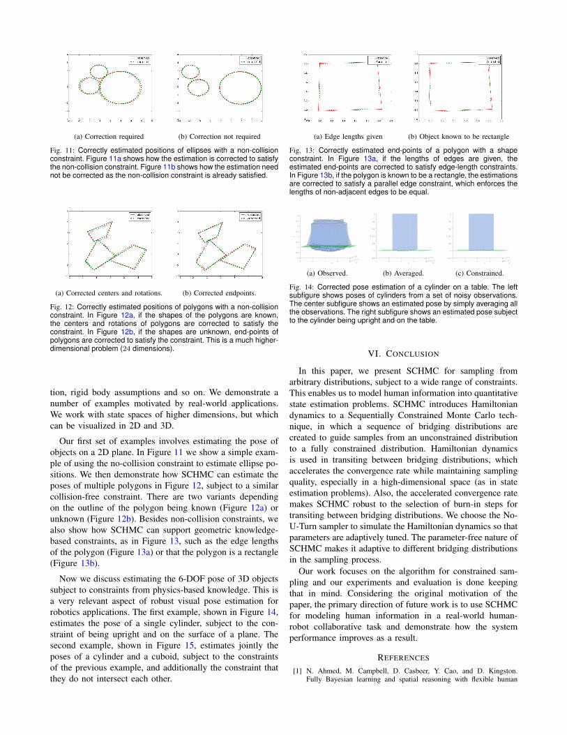
(a) Correction required (b) Correction not required

Fig. 11: Correctly estimated positions of ellipses with a non-collisionconstraint. Figure 11a shows how the estimation is corrected to satisfythe non-collision constraint. Figure 11b shows how the estimation neednot be corrected as the non-collision constraint is already satisfied.

(a) Corrected centers and rotations. (b) Corrected endpoints.

Fig. 12: Correctly estimated positions of polygons with a non-collisionconstraint. In Figure 12a, if the shapes of the polygons are known,the centers and rotations of polygons are corrected to satisfy theconstraint. In Figure 12b, if the shapes are unknown, end-points ofpolygons are corrected to satisfy the constraint. This is a much higher-dimensional problem (24 dimensions).

tion, rigid body assumptions and so on. We demonstrate anumber of examples motivated by real-world applications.We work with state spaces of higher dimensions, but whichcan be visualized in 2D and 3D.

Our first set of examples involves estimating the pose ofobjects on a 2D plane. In Figure 11 we show a simple exam-ple of using the no-collision constraint to estimate ellipse po-sitions. We then demonstrate how SCHMC can estimate theposes of multiple polygons in Figure 12, subject to a similarcollision-free constraint. There are two variants dependingon the outline of the polygon being known (Figure 12a) orunknown (Figure 12b). Besides non-collision constraints, wealso show how SCHMC can support geometric knowledge-based constraints, as in Figure 13, such as the edge lengthsof the polygon (Figure 13a) or that the polygon is a rectangle(Figure 13b).

Now we discuss estimating the 6-DOF pose of 3D objectssubject to constraints from physics-based knowledge. This isa very relevant aspect of robust visual pose estimation forrobotics applications. The first example, shown in Figure 14,estimates the pose of a single cylinder, subject to the con-straint of being upright and on the surface of a plane. Thesecond example, shown in Figure 15, estimates jointly theposes of a cylinder and a cuboid, subject to the constraintsof the previous example, and additionally the constraint thatthey do not intersect each other.

(a) Edge lengths given (b) Object known to be rectangle

Fig. 13: Correctly estimated end-points of a polygon with a shapeconstraint. In Figure 13a, if the lengths of edges are given, theestimated end-points are corrected to satisfy edge-length constraints.In Figure 13b, if the polygon is known to be a rectangle, the estimationsare corrected to satisfy a parallel edge constraint, which enforces thelengths of non-adjacent edges to be equal.

-101x

2

-1

-1

-0.5

0

0.5

1z

1.5

0

2

2.5

3

1y

2 33

(a) Observed.

-101x

2

-0.2

0

-1

0.2

0.4

0.6

z

0.8

1

0 1y

2 33

(b) Averaged.

-101x

2

-0.2

0

-1

0.2

0.4

0.6

z

0.8

1

0 1y

2 33

(c) Constrained.

Fig. 14: Corrected pose estimation of a cylinder on a table. The leftsubfigure shows poses of cylinders from a set of noisy observations.The center subfigure shows an estimated pose by simply averaging allthe observations. The right subfigure shows an estimated pose subjectto the cylinder being upright and on the table.

VI. CONCLUSION

In this paper, we present SCHMC for sampling fromarbitrary distributions, subject to a wide range of constraints.This enables us to model human information into quantitativestate estimation problems. SCHMC introduces Hamiltoniandynamics to a Sequentially Constrained Monte Carlo tech-nique, in which a sequence of bridging distributions arecreated to guide samples from an unconstrained distributionto a fully constrained distribution. Hamiltonian dynamicsis used in transiting between bridging distributions, whichaccelerates the convergence rate while maintaining samplingquality, especially in a high-dimensional space (as in stateestimation problems). Also, the accelerated convergence ratemakes SCHMC robust to the selection of burn-in steps fortransiting between bridging distributions. We choose the No-U-Turn sampler to simulate the Hamiltonian dynamics so thatparameters are adaptively tuned. The parameter-free nature ofSCHMC makes it adaptive to different bridging distributionsin the sampling process.

Our work focuses on the algorithm for constrained sam-pling and our experiments and evaluation is done keepingthat in mind. Considering the original motivation of thepaper, the primary direction of future work is to use SCHMCfor modeling human information in a real-world human-robot collaborative task and demonstrate how the systemperformance improves as a result.

REFERENCES

[1] N. Ahmed, M. Campbell, D. Casbeer, Y. Cao, and D. Kingston.Fully Bayesian learning and spatial reasoning with flexible human

0x

-1-5

0

1z

2

3

0y

5

(a) Observed.

0x

-1-5

0

1z

2

3

0y

5

(b) Averaged.

0x

-1-5

0

z

1

2

0y

5

(c) Constrained.

-5 0 5x

-5

0

5

y

(d) Observed.

-5 0 5x

-5

0

5

y

(e) Averaged.

-5 0 5x

-5

0

5

y

(f) Constrained.

Fig. 15: Corrected pose estimation of a cylinder and a cuboid on a table. 15a shows poses of cylinders and cuboids from a set of noisyobservations. 15b shows estimated poses by simply averaging all the observations. 15c shows an estimated pose subject to the cylinder andcuboid being upright and on the table and they don’t collide. Figures 15d–15f show corresponding overhead views.

sensor networks. In Proceedings of the ACM/IEEE Sixth InternationalConference on Cyber-Physical Systems, pages 80–89. ACM, 2015.

[2] N. R. Ahmed, E. M. Sample, and M. Campbell. Bayesian multicategor-ical soft data fusion for human-robot collaboration. IEEE Transactionson Robotics, 29(1):189–206, 2013.

[3] M. Bocquel, H. Driessen, and A. Bagchi. Multitarget tracking withinteracting population-based MCMC-PF. In International Conferenceon Information Fusion (Fusion), pages 74–81. IEEE, 2012.

[4] M. Brenner, N. Hawes, J. D. Kelleher, and J. L. Wyatt. Mediatingbetween qualitative and quantitative representations for task-orientatedhuman-robot interaction. In IJCAI, pages 2072–2077, 2007.

[5] V. Chernozhukov and H. Hong. An MCMC approach to classicalestimation. Journal of Econometrics, 115(2):293–346, 2003.

[6] R. Daviet. Inference with Hamiltonian sequential Monte Carlo simu-lators. 2016.

[7] P. Del Moral, A. Doucet, and A. Jasra. Sequential Monte Carlosamplers. Journal of the Royal Statistical Society: Series B (StatisticalMethodology), 68(3):411–436, 2006.

[8] S. Golchi and D. A. Campbell. Sequentially constrained Monte Carlo.Computational Statistics & Data Analysis, 97:98–113, 2016.

[9] S. Golchi and J. L. Loeppky. Monte Carlo based designs forconstrained domains. arXiv preprint arXiv:1512.07328, 2015.

[10] D. L. Hall and J. Llinas. An introduction to multisensor data fusion.Proceedings of the IEEE, 85(1):6–23, 1997.

[11] M. D. Hoffman and A. Gelman. The No-U-turn sampler: adaptivelysetting path lengths in hamiltonian monte carlo. Journal of MachineLearning Research, 15(1):1593–1623, 2014.

[12] T. Kaupp, B. Douillard, F. Ramos, A. Makarenko, and B. Upcroft.Shared environment representation for a human-robot team performinginformation fusion. Journal of Field Robotics, 24(11-12):911–942,2007.

[13] W. G. Kennedy, M. D. Bugajska, M. Marge, W. Adams, B. R. Fransen,D. Perzanowski, A. C. Schultz, and J. G. Trafton. Spatial representationand reasoning for human-robot collaboration. In AAAI, volume 7, pages1554–1559, 2007.

[14] Z. Khan, T. Balch, and F. Dellaert. MCMC-based particle filtering fortracking a variable number of interacting targets. IEEE transactions onpattern analysis and machine intelligence, 27(11):1805–1819, 2005.

[15] M. C. Koval, M. R. Dogar, N. S. Pollard, and S. S. Srinivasa. Poseestimation for contact manipulation with manifold particle filters. InIEEE/RSJ Int. Conf. Intelligent Robots and Systems (IROS), pages4541–4548. IEEE, 2013.

[16] L. Kunze, K. K. Doreswamy, and N. Hawes. Using qualitative spatialrelations for indirect object search. In IEEE Int. Conf. Robotics andAutomation (ICRA), pages 163–168. IEEE, 2014.

[17] R. P. Mahler. Statistical multisource-multitarget information fusion.Artech House, Inc., 2007.

[18] M. McClelland, M. E. Campbell, and T. Estlin. Qualitative relationalmapping for planetary rover exploration. In AIAA Guidance, Naviga-tion, and Control (GNC) Conference, page 5037, 2013.

[19] R. M. Neal et al. MCMC using Hamiltonian dynamics. Handbook ofMarkov Chain Monte Carlo, 2:113–162, 2011.

[20] F. Septier and G. W. Peters. Langevin and Hamiltonian based sequen-tial MCMC for efficient Bayesian filtering in high-dimensional spaces.IEEE Journal of Selected Topics in Signal Processing, 10(2):312–327,2016.

[21] D. C. Shah and M. E. Campbell. A qualitative path planner forrobot navigation using human-provided maps. I. J. Robotics Res.,32(13):1517–1535, 2013.

[22] L. L. Wong, L. P. Kaelbling, and T. Lozano-Perez. Collision-free stateestimation. In IEEE Int. Conf. Robotics and Automation (ICRA), pages223–228. IEEE, 2012.

[23] L. L. Wong, L. P. Kaelbling, and T. Lozano-Pérez. Not seeing is alsobelieving: Combining object and metric spatial information. In IEEEInt. Conf. Robotics and Automation (ICRA), pages 1253–1260, 2014.

[24] D. Yi, M. A. Goodrich, and K. D. Seppi. MORRF*: Sampling-basedmulti-objective motion planning. In IJCAI, pages 1733–1741, 2015.

[25] D. Yi, M. A. Goodrich, and K. D. Seppi. Homotopy-aware RRT*:Toward human-robot topological path-planning. In ACM/IEEE Int.Conf. Human-Robot Interaction (HRI), pages 279–286. IEEE, 2016.

[26] D. Yi, T. M. Howard, M. A. Goodrich, and K. D. Seppi. Expressinghomotopic requirements for mobile robot navigation through naturallanguage instructions. In IEEE/RSJ Int. Conf. Intelligent Robots andSystems (IROS), pages 1462–1468. IEEE, 2016.