UPTEC X07 054

Examensarbete 20 pOktober 2007

Model selection criteriain the NOIA framework for gene interaction

Carl Nettelblad

Molecular Biotechnology Programme

Uppsala University School of Engineering

UPTEC X 07 054 Date of issue 2007-10

Author

Carl Nettelblad

Title (English)

Model selection criteria in the NOIA framework for gene interaction

Title (Swedish)

Abstract Existing methods using model selection criteria in QTL analysis were surveyed, and an adaptation for the NOIA (Natural and Orthogonal InterActions) framework, including numerical integration over the model space, was proposed. The new method was validated on experimental and simulated data. Previous results regarding the Bayesian Information Criterion being unsuitable in QTL analysis are questioned.

Keywords Model selection, QTL, junglefowl, chicken, DIRECT, BIC, model averaging

Supervisors

Örjan Carlborg Swedish University of Agricultural Sciences

Scientific reviewer

Sverker Holmgren Uppsala University

Project name

Sponsors

Language

English

Security

ISSN 1401-2138

Classification

Supplementary bibliographical information Pages

39

Biology Education Centre Biomedical Center Husargatan 3 Uppsala

Box 592 S-75124 Uppsala Tel +46 (0)18 4710000 Fax +46 (0)18 555217

Model selection criteria in the

NOIA framework for gene interaction Carl Nettelblad

Sammanfattning

QTL-analys (Quantitative Trait Loci) är ett samlingsnamn på

metoder som syftar till att identifiera positioner i genomet som

kan kopplas till kvantifierbara fysiska egenskaper (fenotyper,

t.ex. kroppsvikt). Detta sker ofta genom att data om specifika

genetiska markörer och de observerade fenotyperna samlas i en

regression.

Det finns ofta fler möjliga positioner i genomet än individer i

experimentet. Detta är också relevant när man försöker se hur

olika gener, på olika positioner, tillsammans påverkar en

egenskap. Varje möjligt par av positioner kan teoretiskt sett ha

en egen påverkan och man kan även bilda grupper med högre

antal.

Detta innebär att det finns oerhört många möjliga modeller,

som dessutom är olika stora. En större modell i en linjär

regression har bättre förutsättningar att beskriva ”bruset” och

därmed uppnå en bra anpassning, men utan att vara biologiskt

relevant. Frågeställningen om vilken modellstorlek som är bäst

kallas modellval. Det finns ett antal enkla kriterier som kan

användas för detta.

I denna studie utvärderades sådana kriterier för QTL-analys,

tillsammans med en beräkningseffektiv implementation av en

ny modell som ger mer biologiskt rimliga parametrar i

modellerna, NOIA.

Civilingenjörsprogrammet i molekylär bioteknik

Uppsala universitet

Oktober 2007

Contents

1 Introduction 1

2 QTL analysis 22.1 Loci, alleles and genes . . . . . . . . . . . . . . . . . . . . . . . . . . . . . . . . . . . . . . . . . . . . . . . 22.2 Heritability . . . . . . . . . . . . . . . . . . . . . . . . . . . . . . . . . . . . . . . . . . . . . . . . . . . . . 22.3 Pedigrees . . . . . . . . . . . . . . . . . . . . . . . . . . . . . . . . . . . . . . . . . . . . . . . . . . . . . . 32.4 A general formulation of the model regression problem . . . . . . . . . . . . . . . . . . . . . . . . . . . . . . 32.5 Interval mapping . . . . . . . . . . . . . . . . . . . . . . . . . . . . . . . . . . . . . . . . . . . . . . . . . . 42.6 MQM (Multiple-QTL-Model) . . . . . . . . . . . . . . . . . . . . . . . . . . . . . . . . . . . . . . . . . . . 42.7 Haley-Knott regression . . . . . . . . . . . . . . . . . . . . . . . . . . . . . . . . . . . . . . . . . . . . . . . 52.8 NOIA . . . . . . . . . . . . . . . . . . . . . . . . . . . . . . . . . . . . . . . . . . . . . . . . . . . . . . . . 62.9 Requirements for orthogonality . . . . . . . . . . . . . . . . . . . . . . . . . . . . . . . . . . . . . . . . . . . 72.10 Deviations from orthogonality . . . . . . . . . . . . . . . . . . . . . . . . . . . . . . . . . . . . . . . . . . . 72.11 A new approach to maintain orthogonality with low genotype information . . . . . . . . . . . . . . . . . . . . 9

3 Model selection 103.1 A Bayesian approach to model selection . . . . . . . . . . . . . . . . . . . . . . . . . . . . . . . . . . . . . . 10

3.1.1 AIC . . . . . . . . . . . . . . . . . . . . . . . . . . . . . . . . . . . . . . . . . . . . . . . . . . . . . 113.1.2 BIC . . . . . . . . . . . . . . . . . . . . . . . . . . . . . . . . . . . . . . . . . . . . . . . . . . . . . 113.1.3 mBIC . . . . . . . . . . . . . . . . . . . . . . . . . . . . . . . . . . . . . . . . . . . . . . . . . . . . 113.1.4 Orthogonality in model selection . . . . . . . . . . . . . . . . . . . . . . . . . . . . . . . . . . . . . . 123.1.5 Integrating over the model space . . . . . . . . . . . . . . . . . . . . . . . . . . . . . . . . . . . . . . 13

3.2 DIRECT . . . . . . . . . . . . . . . . . . . . . . . . . . . . . . . . . . . . . . . . . . . . . . . . . . . . . . . 143.2.1 Search efficiency of DIRECT . . . . . . . . . . . . . . . . . . . . . . . . . . . . . . . . . . . . . . . 143.2.2 Epistasis in DIRECT . . . . . . . . . . . . . . . . . . . . . . . . . . . . . . . . . . . . . . . . . . . . 163.2.3 Using DIRECT for integration . . . . . . . . . . . . . . . . . . . . . . . . . . . . . . . . . . . . . . . 173.2.4 Possible pitfalls in using DIRECT for integration . . . . . . . . . . . . . . . . . . . . . . . . . . . . . 18

4 Simulations 194.1 Genetic architectures . . . . . . . . . . . . . . . . . . . . . . . . . . . . . . . . . . . . . . . . . . . . . . . . 194.2 Further details . . . . . . . . . . . . . . . . . . . . . . . . . . . . . . . . . . . . . . . . . . . . . . . . . . . . 19

5 Biological data 215.1 The data set . . . . . . . . . . . . . . . . . . . . . . . . . . . . . . . . . . . . . . . . . . . . . . . . . . . . . 215.2 Analyses performed . . . . . . . . . . . . . . . . . . . . . . . . . . . . . . . . . . . . . . . . . . . . . . . . . 21

6 Results 236.1 Simulations . . . . . . . . . . . . . . . . . . . . . . . . . . . . . . . . . . . . . . . . . . . . . . . . . . . . . 23

6.1.1 Null models . . . . . . . . . . . . . . . . . . . . . . . . . . . . . . . . . . . . . . . . . . . . . . . . . 246.1.2 Simulated epistasis data . . . . . . . . . . . . . . . . . . . . . . . . . . . . . . . . . . . . . . . . . . 246.1.3 Aggregation methods . . . . . . . . . . . . . . . . . . . . . . . . . . . . . . . . . . . . . . . . . . . . 25

6.2 Biological data . . . . . . . . . . . . . . . . . . . . . . . . . . . . . . . . . . . . . . . . . . . . . . . . . . . 276.2.1 Genome scans . . . . . . . . . . . . . . . . . . . . . . . . . . . . . . . . . . . . . . . . . . . . . . . 276.2.2 Backward-forward selection . . . . . . . . . . . . . . . . . . . . . . . . . . . . . . . . . . . . . . . . 29

7 Discussion 317.1 Important QTLs in experimental data . . . . . . . . . . . . . . . . . . . . . . . . . . . . . . . . . . . . . . . . 317.2 Detection power for different genetic architectures . . . . . . . . . . . . . . . . . . . . . . . . . . . . . . . . . 327.3 The appropriateness of mBIC . . . . . . . . . . . . . . . . . . . . . . . . . . . . . . . . . . . . . . . . . . . . 327.4 Window sizes and filtering . . . . . . . . . . . . . . . . . . . . . . . . . . . . . . . . . . . . . . . . . . . . . 337.5 Factors influencing the computed probabilities . . . . . . . . . . . . . . . . . . . . . . . . . . . . . . . . . . . 347.6 Orthogonality and varying subsets . . . . . . . . . . . . . . . . . . . . . . . . . . . . . . . . . . . . . . . . . 357.7 Conclusions . . . . . . . . . . . . . . . . . . . . . . . . . . . . . . . . . . . . . . . . . . . . . . . . . . . . . 35

A Appendix: Numerical results 36

Bibliography 39

1 IntroductionThis is a study of how to use model selection for detection of Quantitative Trait Loci (Chapter 2) in datafrom line crosses. Several methods have been evaluated using simulated and experimental data from anintercross experiment in chicken. Model selection means, very briefly, methods to determine the mostappropriate model representing the data set, where different models not only vary in parameter values,but also in complexity or scope (see Chapter 3). Here, we focus on evaluating the Bayesian informationcriterion (BIC) (Schwarz, 1978) and the modified Bayesian criterion (mBIC) specifically developed forQTL analysis (Bogdan et al., 2004).

A main question addressed is whether a previous conclusion that the BIC tends to be overly generous(resulting in false positives) in QTL applications, is generally true, or an effect of the properties ofthe specific methods in which it has previously been used. We also introduce weighted integration,or model averaging, over the model space, to get probability estimates in genome scans for QTLs. Inaddition to performing such scans in experimental and simulated data, the theoretical background forthe feasibility of selecting parameters independently of the background of the remaining parameter set,using an orthogonal model appropriate for the data set, was studied. Based on the theoretical results wepropose an adapted method to identify an arbitrary subset of interacting pairs of QTLs from a predefinedset of putative QTLs in experimental data.

1

2 QTL analysisSome properties in individuals, like eye color or the properties in peas originally studied by Mendel, arequalitative, with a finite and relatively small number of distinct classes. This can be contrasted to, forexample, body weight. Body weight is a quantitative trait, i.e. it is generally measured as a real number,on a continuous scale. There is a genetic determination of the trait (i.e. the heritability is > 0), but a moreadvanced analysis is needed to define individual genome locations (Quantitative Trait Loci, or QTL)contributing to the expression of the trait. The actual system will generally have a genetic architecture ofpolygenetic nature, as well as considerable contributions from environmental effects.

It should be noted that even qualitative properties, e.g. cancer incidence, can be studied in a quan-titative genetic framework by assuming an underlying continuous distribution, leading to observed classoutcomes.

The interest in detecting genetic interactions is increasing (Carlborg and Haley, 2004), and so is thegeneral understanding of their importance. This means that individual QTLs, as well as combinations ofalleles in different loci, are studied.

2.1 Loci, alleles and genes

A location in the genome is called a locus (pl. loci). This can be viewed as a specific point (a basepair), but in practice, there is a minimal difference between referring to a particular genome location inbase pairs, or an interval in a limited region. For a specific locus, there can be multiple genetic variants,alleles. The term gene is generally denoting a locus. The main difference is that “locus” focuses onphysical locations in the genome, while “gene” refers to the functional unit that is placed in a locus. Inaddition, not all genome locations are considered to be genes, and some might even be part of multiplegenes.

2.2 Heritability

In quantitative genetics, the concept of heritability is central. The main basis is the concept that theobserved phenotype variance can be decomposed into variances of genetic and environmental origin. Ifthis decomposition is correct and possible, we can compute the ratio between the genetic variance andthe total variance. This is called the broad sense heritability, or h2. The square symbol is motivated bythe fact that variance itself is related to squares.

As variances are additive, this definition of heritability also implies that simulations can be performedby first generating the genetic signal. The genetic variance can then be computed, and an appropriateamount of noise added to generate the desired h2 value.

In biological experiments, h2 can be determined from data on phenotypic traits together with dataon genetic relations between the individuals (e.g. pedigrees). Genomic data is not needed. Data onmonozygotic and dizygotic twins can be one such source for human data. Historically, quantitativegenetics has not been concerned with genes or nucleic material at all, but rather with the different degreesof genetic similarity between individuals.

2

2.3 Pedigrees

QTL analysis can be performed using data from existing populations, e.g. in farm animals and humans.This is generally less powerful than using data from a well-defined experiment cross. Different crossesare used depending on the trait studied and the types of species or lines available.

A standard example of an experimental line cross population is where two inbred lines, that displaydifferent characteristics, for one or multiple traits of interest, are selected as founders. From these lines,an F1 population is bred. The resulting F1 population is expected to be heterozygous in all loci where thelines differ. All individuals will have 50% genetic material from each founder line. The trait differencesin the F1 generation relative to the parental lines can elucidate some information on the genetic structure,but cannot be used to identify individual loci and their effects.

An intercross can be bred from the F1. The resulting F2 individuals have, on average, 50% geneticmaterial from each founder line. Individuals within that population can in theory carry anything from 0to 100% from each founder line. Some loci in the F2 individuals will be homozygous, as both F1 parentscan contribute the same allele to the offspring. As both homozygotes and heterozygotes can be presentfor all loci, the F2 population can be used to identify additive as well as dominance effects of individualgenetic loci.

Backcross populations are also commonly used for QTL detection. F1 individuals are here bred toindividuals from either founder line. This means that one of the alleles in each locus will always reflectthe founder line. Dominance effects from the founder alleles will decrease the observable effects of aQTL in a back-cross, while dominance effects from the alleles transmitted through the F1 line will beseen, but not be distinguishable from additive effects.

In QTL analyses of backcross, only one genotype indicator is needed per locus, and the resulting dis-tribution between the two values, representing the homozygous and heterozygous cases, respectively, isexpected to be uniform 1:1. For F2, at least two genetic indicators are needed, to describe the distributionof the two homozygous genotypes and the heterozygote. The expected distribution is the non-uniformratios of 1:2:1. When covering epistasis (i.e. interactions between genetic loci), the number of indicatorsincrease exponentially with the number of loci included, e.g. 2/3 genotypes per locus (backcross and F2respectively) result in 16/81 genotypes in total in a 4-locus system.

2.4 A general formulation of the model regression problem

The following description is analogous to the one used in Zeng et al. (2005) and Alvarez-Castro andCarlborg (2007).

Let’s assume a population, with known genotypic values (phenotypes) for a trait. These values canbe listed as a vector G∗. If we have data for a set of indicator variables related to genotypes (variousspecific transformations between genotypes at specific loci and the indicator values are possible), thenthe regression of phenotype on genotype can be written as:

G∗ = X ·E + ε (2.1)

where each row in the matrix X represents the realization of the model for the corresponding individualin G∗, expressed as coefficients of the estimated values in E. For example, there will generally be oneparameter in E that is simply the arithmetic mean. Therefore, all rows in X will have a value of 1 inthe column for that parameter, while the columns for the other parameters will shift depending on thegenotype data for each individual.

Different parameterizations can be used, i.e. different mappings between genotypes and what coef-ficients appear in what columns in X , based on the same set of phenotypic observations, and genotypicindicators. One way to formulate this is to make a distinction between a design matrix S, which shouldbe universal for a specific model design (set of indicator variables and parameters), and a matrix Z, that

3

represents the values of the indicators in the population under study, ordered in a way matching G∗.Equation 2.1 will then read:

G∗ = ZS ·E + ε (2.2)

In a one-locus case, the indicator variables in the Z matrix can simply be the presence or probabilityof a 11, 12 or 22 genotype. A multi-locus model can be obtained by taking a row-wise Kronecker productfor design (S) as well as indicator (Z) matrices for the individual loci (described in further detail later).

This approach can also be used to obtain a general genotype-phenotype map, G, from a set of es-timated parameters, in a specific population. This map will simply be an enumeration of the expectedvalues of the trait, over all indicators, i.e. the value expected in an individual with a value of 1, for thatindicator, and 0 for every other.

2.5 Interval mapping

Initially, QTL mapping was concerned only with establishing the mapping between markers and traits.The only indicators present in the regression would be directly related to the genotypes at the markers, andthe marker(s) with the highest explanative power would be chosen. This naturally limits the maximumpower in the detection process, as the actual locus is normally not located exactly at a marker. By onlyconducting analysis at markers, the estimated QTL effect will be underestimated due to recombination.

Lander and Botstein (1989) formulated the first approach to efficiently consider the intervals betweenmarkers. This was done by defining the total likelihood of a model as a product of the likelihoods for eachindividual in the population. The individuals are considered to be mixtures of the possible genotypes.For a backcross, this becomes:

L = ∏i

(Gi0Li0 +Gi1Li1) (2.3)

where Gi j is the genotype probability for genotype j in individual i, and Li j the likelihood (derivedfrom linear regressions) for that genotype and individual. The total likelihood is a product of a weightedcombination of genotype probabilities and the likelihood for the individual cases. This results in a finallikelihood, that can not be computed directly from a simple linear regression.

2.6 MQM (Multiple-QTL-Model)

The approach presented in Jansen (1993), which is generally called multiple-QTL-model (MQM), fol-lows the general description for interval mapping in the previous section, with a modified linear regres-sion model. Multiple loci can be added in the model as separate marginal effects, but also with interactionterms.

The main distinguishing property of MQM relative to other approaches lies in the handling of missinginformation. Missing information occur at marker positions where the genotype can not be unambigouslydetermined, or when QTL genotypes are estimated at non-marker positions.

An expectation-maximization (EM) approach is used, in which expected genotypes and phenotypeparameters are adjusted iteratively. The regression will include rows for every possible genotype, foreach individual. The different realizations are weighted by the conditional probability of the specificgenotype. The probability estimate is based on the present information at flanking markers, and therelation between the observed phenotype value and the estimated phenotype value for that genotype,based on the coefficients in the previous iteration of the EM algorithm.

The estimates of genotypic effects in one EM iteration are used in the following iteration, to updatethe expected genotype probabilities. This results in the phenotypic effects being modified further. Theiterative process is repeated until a suitable convergence criterion is satisfied (i.e. estimates of phenotypiceffects being consistent with estimates of genotype probabilities).

4

The computational demand of MQM is much higher than in comparable methods (e.g. Haley-Knottregression, described below), since a complete computation in those methods, is just a single iterationin MQM. The adjustment of genotype probabilities to match the assumed phenotype effects, against theobserved phenotype, might also increase the sensitivity to overfitting as additional degrees of freedomare introduced. In the degenerate case of no marker information available, MQM and related iterativelikelihood-based, where phenotype information is integrated in the estimated QTL genotypes, methodswill find a “perfect” QTL, for example, unless additional constraints are added.

MQM includes multiple loci in the regression by introducing indicators, far from the locus currentlyanalyzed, as covariates. The motivation for this is an increased power to detect individual loci, by ac-counting for the genetic background (isolating the effects of the loci under study). The matrix designused in the regression can, however, be used without these genetic covariates if desired.

2.7 Haley-Knott regression

Haley and Knott (1992) presented an implementation of interval mapping, where the likelihoods of dis-tinct genotypes are not completely separated. The likelihood in equation 2.3 can not be formulated as alinear regression. In the new approach, the likelihood is approximated through an approximation of thephenotype, as a linear mixture of different genotypes in each individual. The genotype probabilities aredetermined from marker data, and a mapping function (translating mapping distance into recombinationprobabilities).

Each individual is included only once (in contrast to MQM), and if the probabilities are 0.5/0.5for two genotypes, the phenotype will simply be the mean of the estimated effects, of the two alternategenotypes. This has no obvious biological interpretation. The individual should indeed have either onegenotype, or the other, and the marginal expected distribution for phenotypes would not generally matchan assumption of a normal distribution, around the mean of the two underlying possibilites, which iswhat this regression method predicts.

A limited example of this distinction is showed below, with plausible Z matrices, based on the samemarker information, for Haley-Knott and the first iteration of MQM:

ZHK =(0 0.5 0.5

)(2.4)

ZMQM =(

0 1 00 0 1

)In MQM, we get two estimated genotypes, where the RSS influence is weighted by the likelihood

for the genotype itself. Each estimation will include the parameters for that genotype “in full”, though.The Haley-Knott Z matrix, on the other hand, makes a single estimate where the parameters for theheterozygous genotype is included to one half, and the parameters for one of the homozygous cases isincluded to one half. The estimated effect will be an arithmetic mean of the two.

A positive side of the Haley-Knott mixture is that the approximations, while not mapping well toreal world concepts, are “smoothed” in a way. The variance penalty caused by an uncertain genotype inHaley-Knott is lower than the one achieved by simply introducing two rows of equal weight (equivalentto a first-iteration MQM). A more thorough treatment of the differences between Haley-Knott and otherapproaches can be found in Kao (2000).

5

2.8 NOIA

NOIA (Natural and Orthogonal InterActions) (Alvarez-Castro and Carlborg, 2007) is a general modelframework for bi-allelic, multi-locus systems, preferably in linkage equilibrium. Other models, like F2,F∞ and G2A (Zeng et al., 2005) all make specific assumptions regarding the structure of the populationunder study, for the estimated variables to be orthogonal, while NOIA does not. Orthogonality is im-portant to ensure a statistical model where estimates are independent of each other. It is central whenmodel selection is applied as removal of parameters in a model should not influence the estimates of theremaining parameters.

The NOIA model framework includes a change-of-reference operation, allowing the transformationfrom an orthogonal, statistical model into a functional genetic model. This functional model is useful forinterpretations of the predicted effects of individual allele changes in specific genotypes (individuals).

The single-locus design matrix S for an orthogonal bi-allelic single-locus statistical NOIA geneticmodel is: 1 −p12−2p22 − 2p12 p22

p11+p22−(p11−p22)2

1 1− p12−2p224p11 p22

p11+p22−(p11−p22)2

1 2− p12−2p22 − 2p11 p12p11+p22−(p11−p22)2

(2.5)

where pi is the average frequency for genotype i in the specific population studied.For a single-locus model, NOIA maintains orthogonality when there is complete genotype informa-

tion in populations with any combination of genotype frequencies. This is a distinct advantage over theF2 model (only orthogonal for ideal F2 populations), F∞ (orthogonal in a population, without heterozy-gotes and with equal allele frequencies), and G2A (allowing non-equal allele frequencies, but only inHardy-Weinberg equilibrium).

Even in populations expected to be suitable for modelling using F2, F∞ or G2A, NOIA has an advan-tage, as e.g. an experimental F2 population will not show perfect 50/50 allele frequencies, nor Hardy-Weinberg equilibrium, in every locus of the genome. These sampling errors would disappear in asymp-totically large populations, but make usage of a normal F2 model improper in experimental populations,of realistic sizes. NOIA, on the other hand, accounts for actual genotype frequencies in the population,and thus maintains orthogonality.

The Kronecker product can be used to easily construct a multi-locus NOIA model. The Kroneckerproduct is a computation of the element-wise product between two matrices. A n ∗m matrix combinedwith a p∗q matrix results in a (np)∗(mq) matrix. All elements in the left-hand operand are iterated over.The right-hand operand is multiplied with each such iteratee from the left-hand side, and inserted as acontiguous block in the result. An example where the Kronecker product is applied is shown in equations2.10, 2.11, and 2.12.

This symmetrical approach for including multiple loci in the NOIA model also results in one of themodel’s current weaknesses. Although sampling errors in single loci are accounted for, deviations infrequencies for pairs and higher-order combinations of loci, are not handled. In practice, there mightbe a slight over-representation of some multi-locus combinations of alleles. This might lead to a loss oforthogonality, which results in “spilling” of effects, especially if the real underlying effect for one of theloci is strong. This also implies that the estimated effects for one parameter might change greatly, if arelated parameter is removed when model order is altered.

The same argument also applies to linkage disequilibrium, where two loci are located close enoughon the same chromosome to not segregate independently to the next generation. The combinations oflinked alleles found in the parental populations will then be overrepresented in the population understudy. Despite this, the allele frequencies in the loci, when studied individually, might show the expectedproportions. It is important to note that NOIA is currently far from orthogonal, if the sampling errorregarding multi-locus allele frequencies is large, or the loci are closely linked. Further development is inprogress to resolve these problems.

6

2.9 Requirements for orthogonality

A QTL model should ideally be orthogonal when applied to the population studied. In general, anorthogonal matrix is a matrix, where the columns are linearly independent. i.e., for a matrix A, it shouldbe true that:

Ai ·A j = 0 (2.6)

for all i and j, or equivalently, that AAT results in a diagonal matrix.The derivation of orthogonality in appendix C to Alvarez-Castro and Carlborg (2007) is essentially

defining requirements on the design matrix S to satisfy that X should be orthogonal. As X is orthogonalwhen XT X is diagonal, and X = Z ∗S, this is equivalent to ST ZT ZS being diagonal. Here, the derivationassumes that ZT Z can be expressed as a diagonal matrix D, i.e. Z is orthogonal. In the single locus,two-allele case, this becomes:

D = n

p11 0 00 p12 00 0 p22

(2.7)

where pi is the frequency of the 11, 12 and 22 genotypes, respectively. This substitution for ZT Z willhold when there is full marker information, i.e. the QTL genotype can be inferred without error, resultingin mutually exclusive genetic indicators. In this case, Z is orthogonal. Example:

Z =

1 0 00 0 10 0 1

(2.8)

D =

13 0 00 0 00 0 2

3

ZT Z =

1 0 00 0 00 0 2

= 3D

ZT Z is diagonal when Z is orthogonal. All off-diagonal elements are sums of scalar products, betweendifferent rows in the original matrix, and for Z to be orthogonal, all off-diagonal elements in the productwith the transpose should be zero.

2.10 Deviations from orthogonality

Now, consider the case where there is uncertainty in determining the genotype of an individual, e.g. anequal probability for a 11 or a 22 genotype:

Z =

1 0 00.5 0 0.50 0 1

(2.9)

D =

12 0 00 0 00 0 1

2

ZT Z =

1.25 0 0.250 0 0

0.25 0 1.25

6= nD

7

Here, ZT Z is not orthogonal, and D cannot be used to substitute ZT Z in the derivation of an orthogonalmodel (i.e. an orthogonal matrix X = Z ·S). Thus, we have shown that the presence of multiple non-zeroelements, will invalidate the derivation of the orthogonal S matrix. Therefore, it is important to verifywhether the presence of only a single non-zero element per row is preserved, when a multi-locus modelis created through the Kronecker product, given that this property holds for both operands.

If we consider the definition of the Kronecker product, we see that a non-zero element will onlyappear in the intersection between non-zero elements in the factor matrices (Z1 and Z2). For example,consider the following product Z12 from matrices for two loci (Z1, Z2), with full information (i.e. a singlenon-zero element per row):

Z1 =

1 0 00 0 10 0 1

(2.10)

Z2 =

0 1 00 1 01 0 0

(2.11)

Z12 = Z1⊗Z2 =

0 1 0 0 0 0 0 0 00 1 0 0 0 0 0 0 01 0 0 0 0 0 0 0 00 0 0 0 0 0 0 1 00 0 0 0 0 0 0 1 00 0 0 0 0 0 1 0 00 0 0 0 0 0 0 1 00 0 0 0 0 0 0 1 00 0 0 0 0 0 1 0 0

(2.12)

The Kronecker product results in only one single non-zero element in each row in the product matrix,given that each single-locus factor matrix also satisfied this condition.

Only blocks that are multiplied with non-zero elements in the left-hand operand will be non-zero(only one per row), and in those, only one element per row will be non-zero, representing the structureof the right-hand operand. For example, the only non-zero element in the first row is present in the firstblock of three elements, as only the left-most element is Z1 is non-zero. Of the three elements in thatblock, only the second element is non-zero, mapping to the second element in Z2. Although the examplein (2.10), (2.11), (2.12) is given for a two-locus system, the formalism is general for any number of loci.

Incomplete marker information, and sparse marker maps, lead to Z-matrices for individual loci,where there are multiple non-zero elements in each row. As shown above, this leads to a non-orthogonalformulation of the NOIA genetic model (as well as other similar existing models), in the way they arecurrently formulated with missing data. If e.g. Haley-Knott regression is used to estimate genotype prob-abilities, the indicator variables, corresponding to each genotype, will take on real values rather thanbinary integers, reflecting uncertainty in assigning the expected probabilities for each indicator, based onthe actual data for that individual.

The deviation from orthogonality due to lack of unambiguous genotype information, has distinctlydifferent properties from non-orthogonality resulting from the presence of linkage disequilibrium, orsampling errors, as described earlier in Section 2.8. In the latter case, the non-orthogonality is expectedto average out with an increase in population size. The deviations here are only related to the presence ofnon-zero values in multiple columns, in the same row, meaning that increasing the population size willnot cancel this effect. Increasing the genetic information content, by adding more markers, might do so.

8

2.11 A new approach to maintain orthogonality with low genotype infor-mation

Imputations as in MQM (Jansen, 1993) would solve the problem with non-orthogonality due to ambigu-ous genotype information. In an imputation scheme, the single rows with multiple non-zero values arereplaced by several rows, each indicating a single, unambiguous genotype. Weights can then be placedon the rows in the regression.

This scheme will affect the actual value of the residual square sum (RSS), but while a differentapproximation is used, it is not invalid. The weights are placed on complete genotype realizations. InHaley-Knott regression, a mixture genotype is assumed, which contradicts the logic behind separatingthe d (dominance) and a (additive) effects. Such a mixture genotype is a statistical construct, with nocorresponding biological concept.

The choice of imputations also allows the use of a more efficient process to compute the RSS, asdescribed in Ljungberg (2005). Essentially, only a single row is needed for each genotype, so we canachieve results equivalent to those from a model with an infinite number of imputation rows, for eachindividual.

The background to why it is possible to compress all rows of identical genotypes into one, is thatall rows in an overdetermined linear system with the same indicators(/genotype) will, by necessity, havethe same estimated phenotype. Variances being additive, we can compute the variance within that set ofrows and then add them together, resulting in a single row.

Due to the fact that the least-squares regression is exactly that: a reduction of squares, we needto modify the sum slightly; two merged row should only be multiplied by

√2 to get the same relative

weight. For example, if the best approximation of the phenotype is k, and the actual value is m, thenthen RSS for two identical rows is 2(k−m)2. Merging them into one by simple addition would result in(2k−2m)2 = 4(k−m)2, but a single row resulting in the residual square (

√2k−

√2m)2 = 2(k−m)2 is

the appropriate one, showing that a weight of√

2 is indeed correct.In addition to evaluating the RSS in the resulting linear system, the “inner” variances, within each

genotype realization, need to be computed as well. That is a relatively cheap computational operation,compared to an increase in the number of rows in the linear system.

9

3 Model selectionMmodel selection is conceptually a matter of seeking a good balance between fitting the data (explaininga lot of the variance), while not overfitting the data. That is, we want to identify a model that explainsthe underlying reasons for the observations that we made, not just a model where the parameters wereplentiful enough to explain the observations by pure chance.

In some applications, the purpose of a model might be to later perform predictions in conditionssimilar to the ones in the original experiment. Such a model is then only a tool developed throughsupervised training on a data set. Model selection is used to avoid overfitting, while the actual goal is tomaximize prediction accuracy on new observations. If a parameter adds almost nothing to the predictionpower, it is worth including, as long as it does not contribute significantly to overfitting.

Model selection in QTL analysis is a bit different from situations where maximum prediction accu-racy is desired. The evidenced QTLs will be used to derive scientific hypotheses regarding the actualbiological processes behind the trait, hypotheses that might subsequently be verified through experi-ments. The original experiment will probably not be replicated, but it is expected that the results tell ussomething about the genetic influences on the traits studied in the studied population (Fridlyand, 2001).

3.1 A Bayesian approach to model selection

The Bayesian approach to statistics is based on the concept of probabilities. Rather than being a simplematter of frequency counts in sampled data, the probability is in many ways treated as the actual objectof study. An example of this that we can formulate our preconceptions about a situation, before anexperiment is conducted, as prior probabilities.

The model selection problem, or to be more specific, the variable selection problem, in a Bayesianapproach, would properly be computed as the integral of the likelihood of a specific candidate model overall possible values of the variables included in the model, weighted on the probability for each variablevalue. In a genetic model for a trait based on specific loci, the variable values would be the actual geneticeffects. The likelihood, in turn, should be related to the residual square sum (RSS), itself closely relatedto the variance, not only for the optimal solution, but for all possible tuples of variable values.

Note that a model, in this case, is a complete set of loci, not only their number and the types ofallowed interactions. If we impose a 1 cM grid on a 1000 cM genome, this would mean that for 3 loci,we have 109 different models to consider, each consisting of an integral, determining the variance in thecomplete population for “every” possible set of parameter values.

There are several model selection criteria related to Bayesian theory. A crucial assumption for all ofthese is that the likelihood for a model structure can be estimated based only on the regression with theoptimal coefficients. By assuming normal distribution of the possible coefficient values, a regression isused to approximate this, theoretical, integral over all possible values (genetic effects). The underlyingassumption is that it is more computationally efficient and convenient to perform a single regression, thancomputing an integral, that would include evaluating the RSS in every single point.

The derivation of the criteria is also only valid for least-square regression, when errors follow anormal distribution, as this is the requirement for maximum likelihood to be equivalent to least-squares.Recently, ranking methods have also been suggested, to be integrated in model-selection criteria (Zak etal., 2007). This modification intends to avoid the assumption of normal errors.

10

3.1.1 AIC

AIC (Akaike’s information criterion) (Akaike, 1974) is related to information theory and the conceptsof entropy and perplexity. The important point here is that the information content in a dataset relativeto a model is considered to be higher the worse the model is at predicting the data. If the model is ableto predict the data perfectly, we do not gain anything by actually inspecting the data. The informationcontent has a logarithmic relationship to the probability to get the observed data, given the model (mostsimply handled for discrete data, but just as applicable to continuous distributions).

The AIC is based on taking the expectation of the information, and minimizing it, so that the dif-ference between the model and the actual data, is minimized. The parameter values themselves are notdefinite, but only estimations. For a least-squares regression, the criterion is defined as:

AIC = n ln(

RSSn

)+2K (3.1)

where K is the number of parameters, n the sample size, and RSS the residual square sum from a least-squares regression with a specific model.

3.1.2 BIC

The aim of using the AIC is to obtain a model maximizing the ability to predict the observed values ina data set. The BIC (Schwarz, 1978), has historically been derived under the assumption that there is atrue, or correct, model, which should more or less completely explain the variance. The idea is to findamong larger, and smaller, models the one that describes everything. The model is often nested withinlarger models, meaning that the correct model is included in many of the larger ones.

The actual formula for the BIC, in a least-squares regression context, is:

BIC = n ln(

RSSn

)+K ln(n) (3.2)

BIC and AIC contrasted

A result of the difference in rationale behind the BIC, relative to the AIC, is that it imposes a largerpenalty to model size. This implies that one can more freely extend the model set explored, to includemodels that would be highly unlikely to have any biological relevance. The AIC, on the other hand, mightbe prone to overfit to such a model that, while not useful for interpretation of the genetic structure, mightproduce accurate predictions. It has been proved that the AIC does not asymptotically underfit, whileit can overfit, even asymptotically (an infinite number of observations). The BIC will find the correctmodel with an infinite number of observations.

Burnham and Anderson (2002), proponents of AIC in a general sense (while they do not commenton genetic applications), argue that the model set used with AIC should be constrained to models that areconsidered realistic, which would make it impractical for a general search of loci.

Broman (1997) concluded that the BIC, used directly, is too generous with small population sizes,and suggested adding an additional factor δ next to K, and suggested that δ = 2 would be appropriate inmany situations.

3.1.3 mBIC

Bogdan et al. (2004) proposed a modification of the BIC (mBIC), for use in genetic analyses based ongenetic models with pair-wise interaction terms. The aim with mBIC is to introduce priors dependent onmodel size, to give a bound on the expected frequency of false positives (type I errors). This is related tothe work already done in Ball (2001). Both introduce a prior based on the basic combinatorics involvedwhen model size is increasing, in epistatic QTL models.

11

The prior is defined assuming that each main-effect locus has the same probability p to be included.The loci not included then has a probability 1− p. Pairs of loci, are handled analogously, with a probabil-ity p′ and (1− p′) for non-inclusion. The set of possible interaction effects has a quadratic relationshipto the set of main effects.

BIC (3.2) with the prior π(i) would read:

BIC = n ln(

RSSn

)+K ln(n)−2ln(π(i)) (3.3)

π(i) = pa p′b(1− p)(Nm−a) +(1− p′)(Ni−b) (3.4)

where a and b are the number of main and interaction effects, respectively. Now, as BIC is a relativemetric, Nm and Ni terms in the respective exponents can be ignored, as they are constant. Introducel = 1/p,u = 1/p′. The effect of an increase by 1 in a (analogous result for b not shown) is then, basedon (3.4):

∆π(i) =p

1− p(3.5)

ln(∆π(i)) = ln(p

1− p) = ln(

1l

1− 1l

) = ln(1

l−1) =− ln(l−1) (3.6)

Inserting (3.6) in (3.4) gives:

mBIC = n ln(

RSSn

)+(a+b) lnn+2a ln(l−1)+2b ln(u−1) (3.7)

The result here is presented for a backcross (each locus giving rise to one main effect coefficient, andeach included pair resulting in one interaction effect coefficient). l and u are chosen based on the count ofmarkers and the count of marker pairs, with l = Nm/2.2 and u = Ni/2.2, 2.2 chosen arbitrarily with onlya partial justification (Bogdan et al., 2004). Later publications (Baierl et al., 2006) suggest a two-stepprocess where these values of 2.2 are used in the first step, to be adjusted using the tentative results, fora new search in the second step.

3.1.4 Orthogonality in model selection

With an orthogonal model, individual parameters can not only be removed while keeping the regressionresults for the remaining parameters unchanged, the variance is also completely decomposed, with com-ponents mapping to the individual parameters and a residual term. This means that a simple schemeof forward or backward selection, which has been predominantly used in the literature (Broman, 1997;Bogdan et al., 2004; Ball, 2001) can be optimal, if performed as described below:

Forward selection consists of extending a model from a base state (zero parameters, for example),always adding the single parameter that is optimal at that point. Backward selection is an alternativeprocedure that reduces a model from a full state (“all” parameters present), in each subsequent iterationremoving the parameter that results in a minimal reduction of explanatory power. In an orthogonal model,with the decomposition of variance, we can perform the regressions for each parameter in the full modelonce and then rank all parameters by their variance to select a final model including the n highest-rankingparameters.

With a non-orthogonal model, a regression step must be performed in each iteration (i.e. for eachparameter added). Even though forward- and backward selection schemes, based on non-orthogonalmodels, can be optimized, there is a qualitative difference relative to models that are orthogonal, or atleast close enough to orthogonality to be treated as orthogonal in this context. For a forward-selectionapproach on an orthogonal model to be optimal, it is still necessary to consider all parameters in themodel individually. Requiring main effects to be present, before pairwise interactions are considered, is

12

an example of a common restriction in forward selection schemes currently used for genetic mapping,that will lead to a non-optimal result.

NOIA, like other models presently used, is not orthogonal when employed in a Haley-Knott regres-sion QTL analysis, even in the case of linkage equilibrium. This has been discussed earlier from atheoretical standpoint (see Section 2.9).

3.1.5 Integrating over the model space

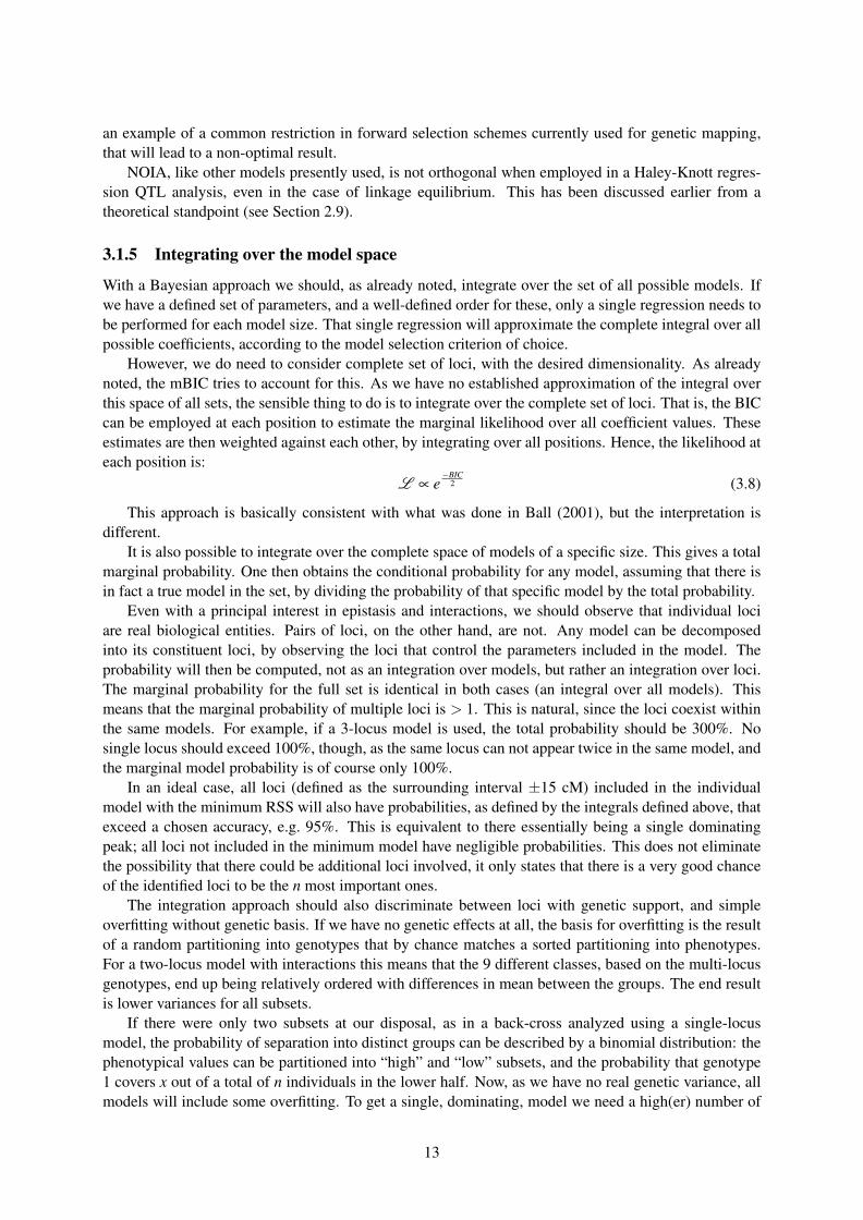
With a Bayesian approach we should, as already noted, integrate over the set of all possible models. Ifwe have a defined set of parameters, and a well-defined order for these, only a single regression needs tobe performed for each model size. That single regression will approximate the complete integral over allpossible coefficients, according to the model selection criterion of choice.

However, we do need to consider complete set of loci, with the desired dimensionality. As alreadynoted, the mBIC tries to account for this. As we have no established approximation of the integral overthis space of all sets, the sensible thing to do is to integrate over the complete set of loci. That is, the BICcan be employed at each position to estimate the marginal likelihood over all coefficient values. Theseestimates are then weighted against each other, by integrating over all positions. Hence, the likelihood ateach position is:

L ∝ e−BIC

2 (3.8)

This approach is basically consistent with what was done in Ball (2001), but the interpretation isdifferent.

It is also possible to integrate over the complete space of models of a specific size. This gives a totalmarginal probability. One then obtains the conditional probability for any model, assuming that there isin fact a true model in the set, by dividing the probability of that specific model by the total probability.

Even with a principal interest in epistasis and interactions, we should observe that individual lociare real biological entities. Pairs of loci, on the other hand, are not. Any model can be decomposedinto its constituent loci, by observing the loci that control the parameters included in the model. Theprobability will then be computed, not as an integration over models, but rather an integration over loci.The marginal probability for the full set is identical in both cases (an integral over all models). Thismeans that the marginal probability of multiple loci is > 1. This is natural, since the loci coexist withinthe same models. For example, if a 3-locus model is used, the total probability should be 300%. Nosingle locus should exceed 100%, though, as the same locus can not appear twice in the same model, andthe marginal model probability is of course only 100%.

In an ideal case, all loci (defined as the surrounding interval ±15 cM) included in the individualmodel with the minimum RSS will also have probabilities, as defined by the integrals defined above, thatexceed a chosen accuracy, e.g. 95%. This is equivalent to there essentially being a single dominatingpeak; all loci not included in the minimum model have negligible probabilities. This does not eliminatethe possibility that there could be additional loci involved, it only states that there is a very good chanceof the identified loci to be the n most important ones.

The integration approach should also discriminate between loci with genetic support, and simpleoverfitting without genetic basis. If we have no genetic effects at all, the basis for overfitting is the resultof a random partitioning into genotypes that by chance matches a sorted partitioning into phenotypes.For a two-locus model with interactions this means that the 9 different classes, based on the multi-locusgenotypes, end up being relatively ordered with differences in mean between the groups. The end resultis lower variances for all subsets.

If there were only two subsets at our disposal, as in a back-cross analyzed using a single-locusmodel, the probability of separation into distinct groups can be described by a binomial distribution: thephenotypical values can be partitioned into “high” and “low” subsets, and the probability that genotype1 covers x out of a total of n individuals in the lower half. Now, as we have no real genetic variance, allmodels will include some overfitting. To get a single, dominating, model we need a high(er) number of

13

x, meaning some degree of separation between the genotypes. The nature of the binomial distributionmakes large deviations of x from the mean highly unlikely.

This is a matter of fringe sampling (within the genome), where the size of the genome determines thesize of the sampling population. As the genome size increases, the expected value of the minimum RSSdecreases, due to chance alone. At the same time, we expect to get more minimas in total, possibly withthe RSS values closer together. An RSS level for which the expected number of peaks is exactly 1, in acertain genome size, will double to 2 if the genome size is doubled. A peak due to the genetic signal willnot show the same behavior, as doubling the genome size in that case means no repeat of the specific setof loci that induced the peak in the first place. Therefore, peaks due to overfitting are expected to showlow probabilities.

3.2 DIRECT

The optimization algorithm introduced for the QTL search problem domain in Ljungberg et al. (2004), iscalled DIRECT. A complete description can be found in that article. A short overview, and some specificremarks regarding the expected efficiency in the optmization search, are found below.

DIRECT is based on a divide-and-conquer approach. The possible QTL locations in a genetic mapare considered to be positions in an n-dimensional space. A particular set of QTLs is defined as a pointin that space. In a traditional exhaustive search, the residual square sum resulting from the model isevaluated in every point of a fine grid in this space (possibly excluding some points due to the symmetryof the search space as the order of the QTL is irrelevant).

DIRECT assumes that the target function (here the RSS of the QTL regression) is Lipschitz contin-uous, meaning that a constant K can be found, such that no partial first-order derivative of the functionf will exceed K in any position. If we accept an approximation where the function is trapezoid betweenthe grid points used in the “ideal” exhaustive search we try to optimize, this is inherent in our definition.

Given a specific value of K, we have a way to define upper and lower bounds for f within any hypervolume. In practice, K is unknown, but we can still impose a partial ordering of volumes or “boxes”. If abox A is both smaller and has a higher RSS than another box B, then no value of K for the whole functioncan give a lower minimum bound within A, than within B.

DIRECT leverages this fact by in each iteration only evaluating those boxes that are included in aconvex hull in the “radius-RSS” space. Larger boxes are thus given “the benefit of the doubt”. Even if theRSS in the centroid (which we have evaluated) might be high, there is a reasonable chance to still find aminimum somewhere else within a larger box. All such candidate boxes are split into three, resulting intwo additional function evaluations (the centroid in one of the boxes remains the same). From an initialbox covering the complete volume, a targeted splitting of boxes, towards the minimum, will take place.

3.2.1 Search efficiency of DIRECT

Asymptotically, DIRECT will evaluate every box. If enough iterations are performed, the result is anexhaustive search. Therefore, we know that the correct box will be found, given enough evaluations. Torealize the benefits of DIRECT over exhaustive search, the value of K should be rather low, or formulatedanother way: the RSS in one point should be a strong indicator of the RSS in the vicinity of that point.Therefore, it is relevant to know how a QTL, defined as the location with a maximum reduction invariance, propagates this effect on the RSS along the genome.

Within a chromosome, the presence of linkage ensures a low K, and most prominently in the presenceof a QTL. If we evaluate the function at the QTL, we can observe a reduction of variance r2, basicallycorrelating to a2, with a being the phenotypic change (consider here only a backcross model) betweenthe two alleles.

A fully informative indicator, at the exact location of a QTL, will be able to absorb all the varianceattributable to that QTL. An indicator at any other location can be related to this indicator by the proba-

14

bility that they match. This relationship is described in more detail below, assuming a simple backcrossdiallelic population.

Asymptotically considering loci far apart on the same chromosome, or loci on different chromo-somes, we have no linkage at all and any match will be random. The probability p of a second indicatormatching an ideal indicator at the QTL will then be 0.5. If the two indicators are identical (infinitelyclose), the p will be 1.0 instead. All other situations are somewhere in between (unless some locus dueto selection pressure actually tends to show an inverted preferred heritage structure relative to anotherlocus).

Assuming that both alleles are equally common in this hypothetical backcross QTL, and that phe-notypic values for the two QTL genotypes are 1 and 0, the variance with a non-parameterized model(average only) will be 0.25. If we use an indicator of the real genotype with accuracy p, we get twosymmetrical classes, each being a mixture of both actual genotypes. Below follows a derivation for thevariance of the “high” one (the one dominated by individuals with a 1 phenotype):

r2 = p(1−µ)2 +(1− p)µ2 = p(1−2µ + µ

2)+(1− p)µ2 (3.9)

µ = 1p+0(1− p) = p

r2 = p− p2

Here, µ is the average value within the class as defined by the indicator. This is the “target” for thelinear regression. As the variance is 0.25 under the null hypothesis, the relative reduction in variancepossible through the indicator is then equivalent to:

0.25− r2

0.25(3.10)

In an actual genome with a known mapping distance x between the loci, p here is equivalent to thecomplement to the recombination fraction. If we assume no recombination interference, we can relatethis to mapping distances, through the Haldane mapping function, with x in cM:

p = 1−0.5(1− e−2x

100 ) = 0.5+0.5e−2x

100 (3.11)

Inserting 3.11 for p in 3.9 and then inserting the result in 3.10, we arrive to a relative reduction invariance of:

e−4x

100 (3.12)

This means that the explainable variance is reduced by a factor of 10, for about every 50 cM (actually57.6 cM). Although not providing a clear guidance on how small the DIRECT boxes need to get, we canquantify the effect on the explainable variance, and see that even at traditionally “unlinked” distanceslike 50 cM, there can a clear signal. On too large a distance, the explainable variance attributable to thelinkage to the actual QTL will disappear, hidden in the noise inherent in the phenotype measurements, andthe fact that the mapping distances are an idealization. The recombination frequencies predicted by themapping function can not faithfully describe the population at every distance. Single “offlier” individualscan affect the RSS greatly, depending on whether they have recombined relative to the genotype at theQTL position, or not.

A practical example of the consequences of the above result would be a population where a singleQTL can just barely be located for a trait with heritability 0.50 (all attributable to this QTL), with amaximum box radius of 100 cM. If the DIRECT parameters are adjusted to a maximum box radius of 40cM, the signal from any possible QTL within the boxes will increase by a factor of more than 10. Thus,any single QTL for a hypothetical trait accounting for a heritability of 0.05 should be detectable. This isbecause the h2 = 0.50 QTL at a distance of 100 cM actually behaves just like a h2 = 0.05 QTL at 40 cM,according to the derivation above. Figure 3.1 also illustrates this, with the heritability of one hypotheticalQTL being half that of another.

15

-50 0 50

Re

lati

ve r

esi

du

al v

aria

nce

Distance from QTL (cM)

Figure 3.1: Example illustrating the explainable variance as a function of distance from the actualQTL, as well as the total explainable variance of that QTL. Two hypothetical cases are shown,with the QTL represented by the dashed line having exactly half the explanation power of the onerepresented by the solid line. If DIRECT reliably detects the dashed line at maximum box radius20 cM in a trait in a specific dataset, then a QTL with twice the power should be detectable withmaximum box radius 38 cM, as both cases result in the same residual variance (connected by thehorizontal line in the graph).

When the true signal is hidden in too much noise, the successive splitting of DIRECT boxes willessentially be “blind” (not having access to any actual indication of what split operations to favor) andapproach the minimum only through an approximation of an exhaustive search strategy. A dataset withmuch noise (through environmental factors or a small population size) will require a higher numberof evaluated boxes (i.e. more DIRECT iterations), to ascertain with reasonable confidence that the trueminimum has been found.

3.2.2 Epistasis in DIRECT

The current DIRECT implementation for QTL searches basically considers the size of the boxes basedon their radius, i.e. the distance between the centroid and a corner, in the multi-dimensional space. Thederivation in the previous section shows how the explainable variance decreases, as a function of thelinear distance from a QTL in a single dimension.

If we perform a multi-dimensional search, the reason can be to identify several QTLs with indepen-dent effects, or to detect an epistatic network. A simple example of the latter would be a case, wherefunctional alleles in multiple loci are needed, for a complete biological pathway to be funtional.

If we have two independent QTLs of equal magnitude, the total reduction of variance when the boxradius is increased is still related to expression 3.10, if we assume that the box centroid is located at thesame distance from both QTLs.

In the case of epistasis (not only multiple main effects), we need an indicator approximating thegenotype at both QTLs. If the distance between the centroid and each genotype lead to an accuracy foreither indicator of p (see Section 3.2.1), the probability that an indicator at this distance represents bothof them correctly (at the same time) is p2.

16

The derivation in the previous section regarding reduction in explainable variance was only directlyrelated to the nature of the genome studied through the definition of p. Therefore, it is possible to plug inp′ = p2 (into expression 3.9) to obtain an expression for the reduction in explainable variance when thegenotypes for two QTLs are needed. This leads to an approximation of the relative reduction in variance(a maximum of 1 at x = 0, x in cM):

e−8x

100 (3.13)

This function declines very quickly. However, this derivation does not take into account that we donot have two symmetrical classes anymore (indicator indicating “high” and indicator indicating “low”),something that would add an additional factor. Furthermore, in the multi-locus case, it is also possiblefor the indicator to be partially correct, representing the genotype at only one locus as “high”. In thatcase, the indicated genotype at the other locus (“low”) might be wrong, with a higher probability thanboth genotypes being wrong in the true “low” case. This partial ignorance about the genotype of eitherlocus corresponds to the main effects of the model. The main effects are the effects that we would see ifwe would only consider either of the QTLs, and be totally ignorant about the existence of the other.

The total explainable variance by the main effects alone in a two-locus architecture in a backcrosswill be about 1/3 of the actual genetic variance. In 1/4 of the cases, both alleles will be “low”, and theestimation can correctly be 0. In 1/2 of the cases, the estimate will be 0.5 (if the true maximum effect is1, one “high” allele will be interpreted as half the effect of two “high” alleles), but the actual effect is 0,since both alleles are required to be “high” to give an actual effect. In the remaining 1/4, the estimatedeffect will be the correct, epistatic effect. This gives a variance of 0 + 0.53 + 0 = 0.125, while the totalvariance is 0.2520.75+0.7520.25 = 0.1875 (the mean is 0.25, 1/4 phenotype 1, 3/4 phenotype 0).

Hence, the main effects will only describe a fraction of the total variance attributable to the QTL, evenat zero distance with perfect genotype information. This means that we can approximate the explainedvariance, as a function of distance, by the maximum of these two briefly motivated functions:

max

(e−

8x100 ,

e−4x

100

3

)(3.14)

This is a very crude approximation as, in practice, both main and interaction effects explain thevariance, at all distances. The different properties imply that one or the other will dominate, dependingon the distance. At long distances, which is what is relevant to decide the maximum allowed size onDIRECT boxes, the main effects term will be the most relevant. It is then important to see that a geneticarchitecture of two-locus epistasis will only result in half the detectable variance, compared to a case oftwo independent QTLs, with the same total explainable variance at the actual QTL positions.

In short, epistatic architectures are more sensitive to a coarse evaluation grid. This sensitivity alsoincreases, with an increased dimensionality of the interactions. This has implications, not only for QTLanalysis based on DIRECT, but also for exhaustive search approaches with coarse grids, or for that matterthe results of varying densities in marker maps.

3.2.3 Using DIRECT for integration

As presented in Burnham and Anderson (2002), there are several reasons for performing an integrationover the model space, to obtain probabilities for individual models, rather than simply searching forthe minimum. Ljungberg et al. (2004) only used DIRECT to identify the single best position in then-dimensional search-space (i.e. combinations of QTL for a pre-defined genetic model).

The similarities between DIRECT and an actual exhaustive search indicate that it should be adaptableinto a numeric integration method. An exhaustive search can be transformed into a (crude) numericalintegration, by assuming each grid point not to be a point, but a volume, where the function value isassumed to be constant. This is a realistic assumption in QTL analysis, as for the exhaustive search to beeffective in the identification of the best fitting model, the points are already assumed to be representativeof their vicinity (if not, the grid is not dense enough).

17

There is a clear difference between DIRECT and many other search algorithms, as for many of these,there is simply no way to decide whether the function evaluations map to suitable bounding volumes,where the function value is representative of the distribution found within that volume.

DIRECT, on the other hand, continuously defines an approximation of the RSS. Potential variationis bounded within each volume explored. The bounding, in addition to the near-zero probability thatresults from the specific variations at values far from the optimum, makes it possible to simply performa summation of the integrand (here, a likelihood estimated based on the RSS), computed for all boxeswhen the algorithm terminates, weighted by box volumes. The error accepted within the bounds of eachbox also controls the total error in the integral.

3.2.4 Possible pitfalls in using DIRECT for integration

DIRECT only considers two things when selecting the boxes to be split further: their radius and thealready evaluated function value at the centroid. The algorithm does not consider any history of thesuccess of splitting neighboring boxes, for example.

In practice, this means that the area around a relative minimum, once found, will be meticulouslyexplored. Even after the minimum has been found, other, and so far relatively unsplit, boxes in thevicinity will be chosen for further splitting. In an application where only the single global minimumis sought, this is a wasted effort. In that case, it is mitigated by the fact that if there exists an optimalminimum, different from the minimum already found, that minimum should allow larger boxes withlower RSS values, and therefore eventually be explored. With high noise levels, that may take long.

In the integration approach, it is possible that the global optimum is found early on, but we still wantto determine whether there is a single, obvious peak. This can only be done by identifying and exploringall sub-optimal regions with RSS values close to the level of the minimum. The RSS value in the veryminimum of those peaks can still be higher than the values in boxes in the vicinity of the global minimum.If the global optimum is then found rapidly, the remaining parts of the search space might be explored inlimited detail. Finding the global optimum is thus a necessary, but not a satisfactory, requirement for theoverall integration to be accurate.

Future extensions of DIRECT specific for use in integration might include solutions to diversifyingthe evaluation grid, as it with the current algorithm is necessary to manually monitor the maximum sizeof the boxes when terminating, as well as perform a far greater number of function evaluations, thanwhen using DIRECT for minimum searches. It is also possible to constrain the minimum radius allowedfor any box, with limited loss in accuracy, as we are unable to discern any relevant data when gettingdown to single cM resolution.

18

4 SimulationsAn F2 population of 1,000 individuals, with a genome of 5 chromosomes of 500 cM each were simulated.The markers were evenly spaced with 10 cM distance. Populations according to these specifications weregenerated at least 100 times, generally about 250.

4.1 Genetic architectures

Three different genetic architectures were evaluated, with two of them including epistasis. The differencebetween the cases is how the loci interact. Hence, there was only a single case for 1-locus architectures,with a single recessive genetic effect. Table 4.1 summarizes the different cases.

All cases are based on recessive architectures within the individual loci. Case C is the only one whereno epistatic parameter terms are expected in the NOIA model. This case has mainly been included toillustrate the kind of models and architectures that have been most prevalent historically.

4.2 Further details

In addition to the genetic signals defined by the three genetic architectures, a normal error was added toresult in h2 (heritabilities) of 0.001, 0.10 and 0.50, respectively. By defining the noise level in terms ofh2, comparisons of detection performance for different architectures can more readily be performed.

10,000 DIRECT iterations, each including multiple function evaluations, were used, to facilitateidentification of all multi-locus genetic signals. A lower number of iterations would generally find thesame minimum, but it might find only that one and completely discard other peaks other than the mostprominent one and thereby invalidate the model space integration.

Model fittings were performed for different model sizes, from 1 to 4 interacting loci. Each model wasunrestricted, i.e. including all the parameters arising from the Kronecker product of statistical NOIA Smatrices for individual loci. An unrestricted model means that a model with 4 loci can describe arbitrary4-way, 3-way, 2-way interactions, as well as single-locus main effects.

19

Table 4.1: Genetic architectures used in simulations. gi is intended to represent the genotype of eachlocus in the architecture. The architectures are generally referenced by ID or name in later sections. Ex-amples of possible biological structures matching these genetic architectures are given in the descriptioncolumn.

ID Name Description Schematic representation ExpressionA All recessive Only two possible signals, “high”

and “low”. The “low” signal willonly show when all involved locishare the same homozygous geno-type, a “(00)n” genotype. This isequivalent to a redundant biolog-ical structure of duplicated genes,where the function is not impaireduntil there is no single allele in thegenome coding for the requiredfunction.

Gene A

Gene B

∧i(gi = 00)

B Total dominance Only two possible signals. The“low” signal will show when atleast one of the loci is homozy-gous for the recessive allele. Thisrepresents a multi-step biologi-cal pathway where the total re-sult is fully dependent on eachstep. This could be represented asa “(00)(xx)n−1” genotype.

Gene A Gene B

∨i(gi = 00)

C Purely additive The presence of a homozygous re-cessive genotype in each locus isrepresented as a separate effect.The biological structure could becompletely separate processes, af-fecting the same phenotypic trait.

Gene A Gene B∑i(gi = 00)

20

5 Biological dataIn addition to the simulations, various model selection criteria were used to study the genetics underlyingbody-weight in an F2 chicken intercross between White Leghorn and Red Junglefowl (Carlborg et al.,2003), where 32 possible QTLs (with either interaction or main effects) were found to reach genomewidesignificance (with a tiered ranking of 5%, 10%, 20% significance levels).

5.1 The data set

A new set of 19 loci were identified, in a two-dimensional genome scan for interacting QTL pairs (ArnaudLe Rouzic, personal communication). The aim in this study was to apply model selection criteria to limitthis set to the subset of effects which have the most pronounced effects on the phenotypic expression inthe data of about 800 individuals.

The traits studied were body weight observed, at 1, 8, 46, 112 and 200 days of age. In addition, theraw (absolute) weight difference, between adjacent sample times, was treated as a separate set of traits,somewhat deceivingly referred to as “growth rates”.

There are substantial correlations between the traits listed above. This was hypothesized to make itdifficult to explore the potentially different biological mechanisms affecting the growth, during differentstages in life. By only considering traits representing the absolute weight, those effects could be hidden.

Therefore, a PCA (Principal Component Analysis) decomposition was made on this set of traits,to obtain a new set of orthogonal and independent traits. The PCA decomposes the values for severalvariables (here trait values) into orthogonal vectors. Furthermore, these vectors are constructed in such away that they are ordered to maximize the explainable variance in the data set. The first PCA componentwill describe the single-dimensional projection along which the maximum amount of variance can beattributed.

Further analysis could then be made on this set of traits.

5.2 Analyses performed

Model selection was performed, using a combined backward-forward selection procedure. The full setof loci was ued, with a model including all pairwise interactions. Individual parameters were removedin a stepwise manner. From a biological perspective, one might naıvely expect for example additive-by-dominance interactions only being present if we also observe main effects, as the general descriptionof the model as a series of deviations make most sense, if we start with simple effects and then addfurther corrections. In a model selection context, this is not applicable. An individual parameter mightbe estimated close to zero in the data. This corresponds to limited evidence for the effect really existing.As the information criteria penalizes the total number of parameters included, the penalty will be evengreater if we want to include all parameters that make logical sense. This penalty will be applied in full,even if only a single parameter from this larger set really leads to any reduction of variance. The modelselection process should therefore ideally focus on only finding the parameters with significant effects,independently of what loci they relate to. The approach of treating all parameters as equivalent opaqueentities is not completely applicable for criteria that take the actual model structure into account (likemBIC), but that is not the case for the AIC or BIC.

21

As NOIA is almost, but not completely, orthogonal, it is reasonable to devise an optimized method,that attempts to reintroduce the removed parameters with regular intervals, but not at every iteration. It isalso possible to cache the already computed effects on the variance, after attempted parameter removalin earlier iterations, thereby allowing some parameters to be ignored as the results from earlier iterationsmay show them to conclusively be suboptimal, even at the current iteration.

These two changes imply that the complete parameter space does not have to be explored at each stepwith a very limited loss of generality, but a significant increase in performance.

The backward-forward selection was augmented with genome scans for full models up to 4 loci,employing the methods described in Chapter 4. These scans were complete, i.e. not restricted to the pre-determined set of possible QTLs. Here, a low cutoff probability of about 20% was used, to give moreinsight into the data, especially as there is no preknown list of correct loci to compare against. The BICwas also applied to these results.

22

6 ResultsAll results were obtained by using a modified version of the software originally written by Kajsa Ljung-berg (Ljungberg et al., 2004; Ljungberg, 2005), including implementations of efficient methods for QTLscans and evaluation of the RSS for regression at putative QTLs. The code, written in C, was modified toaccomodate the NOIA model framework, and added flexibility concerning the number of loci involvedin the model.

6.1 Simulations

All random numbers were derived from the Mersenne-Twister pseudo-random number generator withdefault parameters from the Boost package (Boost C++ Libraries 1.34.1, 31 Jul. 2007). This allows com-pletely repeatable runs to be performed, assuming that the same Boost version is used, to avoid artifactsfrom the rather rudimentary pseudo-random number generators present in standard C(++) libraries.

Two performance metrics were used for evaluating the model selection procedure: false detection rate(FDR) (Zak et al., 2007) and power. These are defined below, but can in general be considered analogousto precision and recall, which are used in mainly the domains of AI and natural language processing, orselectivity and specificity, in medicine.

The detection power is defined as the fraction of “real” simulated loci that were reported by themethod. A number of 1 would indicate a perfect result, while a number of 0 would be poor (even slightlyworse than random chance). Our definition of a correct match is equivalent to the one used in the originalarticles on mBIC and rBIC, i.e. a window of ±15 cM around the specific simulated locus. Differentwindow sizes were tested on smaller datasets. The results indicate that the window size is not critical forthe results presented, under the current experimental conditions.

The FDR is defined as the fraction of incorrectly identified loci, among those identified in total:

FDRi =FPi

ci +FPi(6.1)

where ci is the number of correctly identified loci, FPi the number of “false positives”, i.e. loci reportedas part of the model that were not included in the simulated data. If the denominator (and numerator) areboth zero, FDRi is defined as zero as well. FDR is then computed as the average over all FDRi. Hence,the FDR will not be proportional to a simple sum over the number of false positives in all models.

Power and FDR values are summarized, for different model sizes and actual number of interactingloci, in Figures 6.1 and 6.2 and Tables 6.1, A.1, and A.2. The cutoff value used for inclusion of a locuswas consistently 95% probability, as determined by integration over all models, where the locus wasincluded, and divided by the marginal probability over all models (see Section 3.1.5).

These results are then improved by employing aggregation (i.e. model selection criteria for the mod-els of different size) in the end of this section, and analyzed in the discussion.

23

6.1.1 Null models

No null models were technically used in this study, but the simulations based on a h2 of 0.001 proved togive practically no detection for any model size. The detection power, if it even should be considered,was at most 4.1%. This was obtained with 4-locus models, and is close to the expected random rate of1.2% (genome size by window size) per locus included (or 4.8% for 4 loci, if they would be independent).The FDR is presented for all model sizes in Table 6.1.

Table 6.1: False detection rate for null models (h2 = 0.001)

Size of regression model (loci) FDR1 0.4%2 2.9%3 13.4%4 44.8%

6.1.2 Simulated epistasis data

For case A (all recessive, reference Table 4.1), 240 simulations were performed for 1 and 2 loci, and120 simulations for 3 loci. For case B, 300 simulations were performed, while 250 simulations wereperformed for case C.

The FDR increases with an increase in model size. This is most obvious in models where the truegenetic architectury is comprised of a low number of loci (Figures 6.1 and 6.2). With a high heritability,the detection power always approaches 90.0%, with some distinct differences between architectures A,B, C. An overparameterized model will not decrease the power of detection by much, while a model sizematching the actual number of loci in the architectures is optimal.

0

5

10

15

20

25

0

20

40

60

80

100

1 2 3 4

FDR

(%

)

De

tect

ion

po

we

r (%

)

Model size (# of loci)

Power, 1

Power, A

Power, B

Power, C

FDR, 1

FDR, A

FDR, B

FDR, C

Figure 6.1: Power of detection and False Detection Rate (FDR) for architectures A, B, C (Table 4.1)for 2 simulated loci, and the single 1-locus case, h2 = 0.10. FDR is scaled by a factor of 4 to betterillustrate the differences.

The power of detection for 2-locus architectures is low in a 1-locus model, even when consideringthat the maximum theoretical power for 2 loci in a 1-locus model would be 50% (Figure 6.1). This effectis even more pronounced in 3-locus architectures, especially for case A (Figure 6.2). The power in themodel size 1 case is equivalent to the first locus detected in a naıve forward-selection method.

24

0

5

10

15

20

25

0

20

40

60

80

100

1 2 3 4

FDR

(%

)

De

tect

ion

po

we

r (%

)

Model size (# of loci)

Power, A

Power, B

Power, C

FDR, A

FDR, B

FDR, C

Figure 6.2: Power of detection and False Detection Rate (FDR) for architectures A, B, C for 3simulated loci, h2 = 0.10.

Refer to Table A.1 in the appendix for the numeric values of power and FDR on which the figuresare based. This includes the values for h2 = 0.5, which are generally similar, the main difference being amarkedly higher (> 85%) power of detection with 3 simulated loci in cases B and C.

6.1.3 Aggregation methods

The results above are presented independently for each model size. By using integration with a sig-nificance threshold, it is, for example possible to get less than 4 significant loci from a 4-locus model,for example. To actually be reported, a locus still needs to be included in models with a probability of95%, related to the integral over all models of that size. To consistently use the largest model wouldnevertheless limit the accuracy as FDR, but also the detection power, deteriorates.

What is needed is a way to aggregate these independent results, by using a model selection criterion.A very simple criterion, specific for this method, would be to only select a model size if all loci ina n-locus model are classified as significant by the integration method. This is a form of consistencyrequirement. If the model type is not internally consistent in specifying a result matching its dimension,this line of reasoning says it does not make sense to choose it. Therefore, we call this the consistencycriterion (CC). For a series of different model sizes, one should then choose the largest size whereconsistent results were obtained (i.e. n significant loci detected for size n). This criterion can be usedwithout any further information on the actual structure of the models, including their parameter count.

We can also employ the BIC and AIC. Here, we also need to introduce the implicit null model as anoption. The AIC/BIC value for the null model is related to the RSS for a model resulting in the originalvariance in the data set.

The actual model (the left-most bar in Figures 6.3 and 6.4) indicates the result for a model sizematching the number of loci simulated, and can be contrasted against results for CC, BIC and AIC.

The AIC gives an unacceptably high FDR in all configurations, with only negligible gains in detectionpower. The CC and BIC are overall quite comparable. For the 3-locus simulations with h2 = 0.10, bothCC and BIC drops off dramatically in detection power, but BIC more so. For case A, the BIC detectionpower is only 22.8%, while it is 79.4% for CC and 91.1% for AIC with the size 3 model. With a higherheritability, the FDR increases, but the BIC stays competitive in matching the performance of the actualmodel in all simulations. The complete set of results can be found in the appendix, Table A.2.

25

Act

Act

Act

Act

Act

Act

Act

CC

CC

CC C

C

CC

CC CC

AIC

AIC

AIC

AIC

AIC

AIC

AIC

BIC

BIC

BIC B

IC

BIC

BIC B

IC

0

5

10

15

20

25

0

20

40

60

80

100

1 locus 2 loci, A 2 loci, B 2 loci, C 3 loci, A 3 loci, B 3 loci, C

FDR

(%

)

De

tect

ion

po

we

r (%

)

Figure 6.3: Power of detection and False Detection Rate (FDR) for architecutres A, B, C (Table 4.1)with h2 = 0.10. Black bars indicate FDR (right axis), while the white bars indicate detection power.Act = model size matching number of simulated loci, CC = Consistency criterion, AIC = Akaikeinformation criterion, BIC = Bayesian information criterion.

Act Act

Act

Act

Act

Act

ActC

C CC

CC

CC

CC

CC

CCA

IC

AIC

AIC A

IC

AIC

AIC

AICBIC BIC

BIC

BIC

BIC

BIC

BIC

0

5

10

15

20

25

0

20

40

60

80

100

1 locus 2 loci, A 2 loci, B 2 loci, C 3 loci, A 3 loci, B 3 loci, C

FDR

(%

)

De

tect

ion

po

we

r (%

)

Figure 6.4: Power of detection and False Detection Rate (FDR) for different architectures withh2 = 0.50. Bars and categories defined in Figure 6.3.

26

6.2 Biological data

6.2.1 Genome scans

Genome scans were performed in the Red jungle fowl x White Leghorn F2 intercross, with a methodologysimilar to the one described and used in the simulations section (i.e. full models with size 1 up to 4, al-lowing interactions up to the order of the model, and integration by DIRECT to determine probabilities).Table 6.3 summarizes the results for a variety of traits and model sizes.

In Table 6.2 the results from applying BIC to the resulting models is demonstrated. Only a lowthreshold was used to filter the loci listed, which should be contrasted to the strict 95% threshold in thesimulations section. For Bw1 and PC3, the number of loci explodes when model size 4 is reached. Thisfact can indicate overfitting, but it could also be interpreted as the presence of two relatively independentinteraction networks influencing the trait.

We can note very distinct differences between the different models regarding the proportion of vari-ance attributable to the loci included in the genetic models. PC1, which is designed to be a scalarexplaining much of the total trait variance, also seems to have a high genetic basis.

The raw (non-PC) traits only show a single significant locus. Despite this, the same set of 3 loci(1:100, 1:430, 1:485, chromosome number:location on chromosome (cM)) appear multiple times in thetraits related to body weight between 46 and 200 days of age. Two of these (1:100, 1:485) are also thesame ones found to be significant for PC1. There is no indication that the BIC is overall too generous,although the single Bw1 QTL found is indeed very weak (only 1.8% explained variance).

Table 6.2: Explained variance, and loci chosen by BIC, for the traits and model sizes analyzed. Theportion of explained variance relative to the maximum, and the size of the model (the parametercount) are the only two factors affecting the BIC. The results are very restrictive in all cases. Notethat the portion of explained variance here should be expected to be higher than the “actual” geneticvariance, as some degree of overfitting is always possible and present.

Model size 0 1 2 3 4 Number of lociTrait Explained variance chosen by BICBw1 0.0% 1.8% 3.8% 7.7% 15.7% 1Gr18 0.0% 4.9% 8.4% 13.1% 19.8% 1Bw8 0.0% 4.4% 7.3% 11.4% 19.4% 1Gr846 0.0% 11.3% 13.7% 16.8% 23.8% 1Bw46 0.0% 12.0% 14.5% 17.5% 24.3% 1Gr46112 0.0% 6.8% 10.0% 13.6% 21.1% 1Bw112 0.0% 9.6% 13.0% 16.6% 23.4% 1Gr112200 0.0% 5.4% 8.1% 11.8% 19.8% 1Bw200 0.0% 9.0% 12.4% 16.1% 23.4% 1PC1 0.0% 26.6% 33.2% 36.7% 42.4% 2PC2 0.0% 1.5% 4.6% 8.9% 17.8% 0PC3 0.0% 2.2% 4.9% 9.4% 16.9% 1

27

Tabl

e6.

3:D

etec

ted

loci

,with

wei

ght(

prob

abili

ty)c

ompu

ted

byin

tegr

atio

nov

erth

eop

timiz

atio

nla

ndsc

ape

forB

w(b

ody

wei

ght)

,Gr(

grow

thra

te,d

iffer

ence

betw

een

two

mea

sure

dbo

dyw

eigh

ts)

atdi

ffer

entn

umbe

rof

days

afte

rha

tch,

and

the

first

thre

epr

inci

palc

ompo

nent

s(P

C).

Loc

idefi

ned

asch

rom

osom

enu

mbe

r:lo

catio

non

chro

mos

ome

(cM

).

Trai

tB

w1

Gr1

8B

w8

Gr8

46B

w46

Gr4

6112

Bw

112

Gr1

1220

0B

w20

0PC

1PC

2PC

3M

odel

Size

Loc

usPr

ob.

Loc

usPr

ob.

Loc

usPr

ob.

Loc

usPr

ob.

Loc

usPr

ob.

Loc

usPr

ob.

Loc

usPr

ob.

Loc

usPr

ob.

Loc

usPr

ob.

Loc

usPr

ob.

Loc

usPr

ob.

Loc

usPr

ob.

17:

075

68.2

%1:

143

90.9

%1:

105

68.3

%1:

104

100.

0%1:

101

100.

0%1:

104

100.

0%1:

104

100.

0%1:

130

99.7

%1:

104

99.9

%1:

096

100.

0%20

:045

25.1

%1:

111

73.2

%1:

144

31.7

%

27:

075

76.3

%1:

144

96.2

%1:

147

64.1

%1:

103

99.8

%1:

102

99.8

%1:

104

99.8

%1:

104

99.8

%1:

135

99.9

%1:

103

99.8

%1:

483

100.

0%1:

137

69.1

%1:

112

95.1

%8:

063

65.6

%8:

065

49.6

%1:

480

58.5

%1:

480

70.6

%1:

486

92.7

%1:

486

99.6

%4:

168

32.8

%1:

486

93.9

%1:

095

99.9

%11

:014

67.1

%27

:023

86.5

%1:

104

38.1

%1:

014

28.0

%8:

014

37.4

%

37:

075

88.6

%1:

143

100.

0%1:

147

92.8

%1:

104

99.6

%1:

104

99.1

%1:

104

99.6

%1:

482

99.8

%1:

139

100.

0%1:

098

99.7

%1:

481

100.

0%1:

137

84.3

%17

:046

100.

0%14

:014

56.0

%5:

152

65.5

%8:

068

78.0

%1:

488

60.3

%1:

480

63.1

%1:

489

81.6

%1:

101

99.6

%4:

168

64.0

%1:

487

98.9

%1:

095

99.8

%11

:017

82.4

%11

:048

94.3

%1:

411

36.4

%3:

154

56.1

%1:

479

76.3

%1:

434

64.3

%1:

434

86.0

%24

:014

44.6

%1:

425

70.4

%3:

163

94.1

%4:

170

81.9

%1:

452

92.4

%8:

065

37.3

%1:

482

26.6

%

47:

074

52.2

%1:

144

100.

0%1:

144

98.4

%1:

104

98.0

%1:

101

97.6

%1:

432

99.4

%1:

098

98.3

%1:

139

97.2

%1:

431

100.

0%1:

094

100.

0%1:

139

96.6

%1:

453

52.8

%1:

249

48.1

%8:

068

94.8

%3:

145

52.3

%3:

215

46.3

%28

:036

56.9

%1:

491

97.9

%1:

433

98.3

%1:

432

91.4

%1:

482

100.

0%1:

481

100.

0%7:

016

96.2

%11

:048

48.5

%2:

216

48.0

%1:

481

53.5

%15

:042

50.8

%9:

019

45.3

%20

:014

36.0

%1:

098

97.3

%1:

483

97.6

%24

:014

89.8

%1:

096

99.8

%3:

162

96.5

%32

:-15

92.0

%32

:-15

45.1

%14

:014

45.7

%3:

146

35.2

%3:

250

50.4

%1:

195

45.1

%4:

068

34.8

%17

:046

92.9

%17

:046

60.3

%13

:059

69.3

%29

:008

95.5

%27

:023

96.4

%8:

068

90.7

%7:

094

43.5

%1:

378

45.7

%7:

056

28.9

%1:

413

44.5

%28

:036

29.4

%20

:014

28.0

%4:

166

37.8

%2:

234

43.1

%11

:048

45.4

%5:

152

27.5

%10

:080

44.5

%1:

114

43.0

%4:

141

44.9

%7:

059

38.4

%2:

330

42.9

%26

:014

44.6

%29

:008

42.1

%

28

6.2.2 Backward-forward selection

17 of the 19 loci detected in the pairwise scans were used in the backward-forward selection experiements.These are presented in Table 6.4. Two of the loci in the original set provided were removed, due to stronglinkage to loci already present in the set (1:139 and 27:0).

Table 6.4: Loci used as initial basis for backward selection with termination determined byBIC. Normal read order (left to right, then top-down). Locis are denoted by chromosome num-ber:chromosome location (cM).

Locus Locus Locus1:102 1:486 2:1543:025 3:172 4:1515:014 5:081 6:054

11:059 12:040 13:05016:001 17:059 20:00120:040 27:008

The backward-forward scheme first includes all parameters, for main effects and pairwise interactionsbetween the loci in Table 6.4, in the model, and iteratively removes the parameters with the lowest effecton the variance.

Table 6.5 presents the sets of loci included in the models and the resulting parameter values (effects)according to the model, for each of the traits PC1-PC3. Parameter IDs are composed of the loci underly-ing each parameter, ordered as in Table 6.4, with “a” indicating an additive effect and “d” a dominanceeffect. A period indicates a reference effect, i.e. a locus that is not involved. The specific effect valueshere are naturally arbitrary, and the traits themselves quite opaque. The interesting aspect is the distri-bution of magnitudes in effects, and the frequent switching in sign between main effects and epistaticeffects.

We can also observe that there is no clear overlap between the parameters chosen here, and the set ofloci detected in the genome scans for the same traits. The genome scans allow higher-order interactions,but also only accomodate full models. The models presented here are actually comparable in size with afull size 3-model, while involving a far higher number of loci. Thus, most of the loci from the originalset are represented for each PC trait, but frequently by only a single parameter each.

29

Table 6.5: Parameter IDs and effect values for BIC-chosen models for PC1, PC2, and PC3, byusing the backward-forward selection method. The letters a/d indicate additive, dominance effects,respectively. The letter position in the ID should be interpreted as the corresponding locus in Table6.4 (read left-to-right, top-down). Quite a few epistatic parameters are remaining in the resultingmodels.

Parameter ID PC1 Effect PC2 Effect PC3 Effect................. −0.014 −0.003 0.018................a −0.410 - −0.346..............d.d - −1.108 -............ad... - - 0.473...........a....d - −0.618 -..........a...... - - −0.228..........da..... - 0.688 -.........a....... −0.310 - -........a........ −0.356 - 0.270........ad....... 0.661 - -........d...d.... - - 0.887.......a......... −0.407 - -.......a.....a... - 0.557 -......a.......... −0.336 0.323 -......a.........a - −0.585 -......a.a........ - - 0.474......aa......... 0.464 - -......d........d. - - −0.844......d.......d.. - −1.273 -.....a........... −0.242 - -.....a...a....... 0.479 - -.....d.......a... - 0.518 -....a............ −0.390 - -....d.....a...... - 0.588 -....d.a.......... −0.720 - -...a............d 0.795 - -..a.............. −0.894 - −0.255..d...........a.. - - 0.474..d..........d... −1.153 - -.a............... −0.627 −0.310 -.a.......d....... - −0.698 -.d...........d... 0.937 - -.d...a........... - −0.465 -a................ −1.521 - −0.319d................ −0.486 - -d.............a.. - −0.530 -d......a......... - 0.673 -d......d......... - 0.870 -d...a............ 0.627 - -d...d............ - - −0.641

30

7 Discussion

7.1 Important QTLs in experimental data

Although the main purpose of this study was to evaluate the model selection criteria and methods de-scribed in the introduction, primarily based on theory and computer simulations, the experimental studyis a case example that gives additional insight, for example into the effects of covariates and varyingcutoff (“significance”) values.

The most important conclusion for the analyses based on experimental data, is that the BIC is veryrestrictive when utilized in genome scans to detect QTL. For all traits but PC1, the BIC results indicatethat no loci, or only a single locus, significantly influence the trait. Despite this, we have identified threeloci (in Table 6.3, approx. 1:100, 1:430, and 1:485) that are displayed in size 3 models for Gr46112,Bw112, Bw200. Note that these loci were not identified for Gr112200, possibly indicating that these locihas a more pronounced effect on the development up to 16 weeks of age (112 days). Two of them alsoappear in the 2-locus model for Bw8, and the 3-locus models for Gr846 and Bw46.

The fact that these 3 loci are consistently reported indicates that the loci found might not be the resultof simple overfitting of noise. If they are in fact spurious (and the BIC interpretation true), this wouldmean that, somehow, the genotypes in these loci map well to some common environmental factors orother covariates, giving a similar effect for all measured traits. Therefore, a more plausible conclusionwould be that the BIC is overly restrictive in this case.

While there is no way to verify the “true” number of QTLs within the scope of this study, the size 4models for real data do not demonstrate the same consistency between different traits. In fact, they even“lose” several loci consistently reported in the smaller models. Considering the fact that full models wereused (resulting in 3 times the number of parameters in size 4 vs. size 3) it is plausible that model size 4is subject to overfitting in the current data.

Two of the three common loci in the size 3-models for multiple traits (1:100, 1:485), were also presentin the pairwise genomewide scans, based on different methodology, that underlie the locus set used inthe backward-forward selection. A strong pairwise interaction was implicated between these two, forthe traits Gr846, Bw46, Gr46112, Bw112, Bw200 (Orjan Carlborg, unpublished data). Many of the locireported in size 3 models for the PC traits, are also reported in the results underlying the selection of thatsubset, even including reported interactions between the loci.

The 1:430 locus, on the other hand, is not present in this alternate set based on another method. Thiscan be due to imposed limits on closely linked loci, rather than an actual absence of the effect. A weak1:404 locus was present in the results from the other scan method, while not strong enough to be includedin the set of 17 used in the backward-forward method. That locus demonstrated some interactions, withother loci not specifically picked up in the scans made in this study. It is possible that the genetic effectsrelated to 1:430 are only manifested when combined with 1:485 and 1:100, while we cannot rule out thepossibility that its presence here is due to artefacts related to linkage. It is still clear that the BIC result,of only a single significant locus per trait, is overly restrictive.

31

7.2 Detection power for different genetic architectures

Figures 6.1 and 6.2 show clearly that the detection power varies greatly depending on the genetic archi-tecture, including the number of loci involved. This is especially interesting since the total heritabilityattributable to the simulated genetic architectures is kept unchanged, unlike in some other studies.

The most obvious demonstration of this is found in case A (all recessive, see Table 4.1). When themodel fitted to data is too small to accomodate the number of simulated loci, the detection power isdrastically reduced. This is not just some theoretical case, but a fact of tremendous importance. Manyexisting QTL search methods will perform forward selection or a genome-wide scan for only single locior pairwise interactions. A forward selection strategy will not be able to find an unambiguous minimumin the correct position in the first iteration. Even seemingly more general Bayesian approaches, basedon MCMC (Markov-Chain Monte Carlo), will generally only change the model size in limited steps,and so the search to identify the posterior probabilities might never discover the true optimums, wheninteractions are important. However, the low power reported here (2.2%) is only partially a result fromthe genotypes being rare. All three interacting loci will have similar genetic effects and therefore sharesimilar probabilities. This results in no single locus reaching the cutoff of 95%.

To analyze the effects of the cutoff further, the single most important peak (ignoring whether itexceeded the cutoff) in each fitting of a size 1 model, to case A, 3 loci, h2 = 0.50, was listed. In 51.7%of the cases, one of the three simulated loci was chosen. As no cutoff was used, all cases withoutcorrect results were incorrect, to be contrasted against the case in the results section, where the FDR anddetection power do not sum up to 100%. A forward selection process, where only single loci are addedat a time, would match these results in the first iteration. By using pairwise addition steps, the proportionof correct loci added in the first step increases to be 81.7% (18.3% FDR), whereas 91.1% (1.7% FDR) isreached, when a three-locus model is used, with a cutoff.

Different genetic architectures result in different absolute effect magnitudes, related to the standarddeviation of the noise component. An architecture with rare effects (e.g. the completely recessive caseA) results in large phenotype deviations in a small amount of individuals that contribute to the geneticvariance.

7.3 The appropriateness of mBIC

The unmodified BIC performs well in our simulations, when combined with an integration (model aver-aging) approach. This contradicts earlier findings that BIC is overly generous in genetic model selection(Broman, 1997; Bogdan et al., 2004). The application of BIC to experimental data support what wefound in the simulations, as it appears to be overly restrictive for those data when compared with resultsfrom other analyses of the same data. An integration over different sizes could possibly alleviate this.Our simulation study show that detection power, and FDR, when using BIC are comparable to thoseobtained using mBIC (Bogdan et al., 2004). Our results therefore indicate that the general conclusionthat the unmodified BIC is unsuitable for genetic model selection, does not hold.

The prior in mBIC (Bogdan et al., 2004) might seem sound at first, as an increase in the number ofpossible models increases the risk that a good model is found by overfitting. There is, however, onlya weak correlation between increasing model size and a good model fit by overparameterization. Adoubling of the model space will not lead to a model that is twice as good at explaining the data, bychance. The vast majority of models, no matter what space we sample from, will have minimal supportin the data.

To understand this, one can think of differences in model size as a matter of sampling from the samedistribution, as the RSS value for possible models can be viewed as a distribution. The very best modelis part of the fringe of this distribution. Doubling the model space is then only equivalent to doubling thepopulation size in the sampling process. The actual position of the fringe will not move by doubling thesampling population, but the most extreme individual found can shift slightly.

32

The sampling interpretation has greater consequences when considering interactions, which is themotivation for developing the mBIC. The mBIC prior, as noted (Section 3.1.3), basically considers thatthere are n2 possible interaction terms if there are n possible additive terms. The mBIC then states thatthe fit, when including interactions, should be n2 times “better” to be preferred, in addition to the directpenalty induced by the BIC through the number of parameters and the resulting degrees of freedom.

If all models of the desired dimension are considered, then this high penalty might be deemed ap-propriate, but the authors advocate using the prior described in a context where only a single model ischosen. In that context, the total dimensionality is irrelevant. Even in the case of considering all models,we should only compensate the added volume of the peak due to the added dimensionality, not for theincreased volume of the model space in full. Further studies are needed to describe the distribution ofRSS values.

Although we used integration for each individual model size in this study, the model selection criteriawere only applied to the minimas. The approach thus still focuses on the minimum found, but uses thecomplete optimization landscape to determine how that minimum should be interpreted once the modelhas been selected. Integrating over all model sizes and models would make more sense, but require alarger change in the implementation. One could also argue that, once smaller models are ruled out asinaccurate, they should not influence the probabilities at all. It would be interesting to explore whetherthe cases of very high FDR (especially for h2 = 0.50), reported in some cases, could be reduced by usinga “full-integration” approach, without losing the high detection power.

The high false-detection rate of unmodified BIC reported in the literature (Bogdan et al., 2004; Bro-man, 1997) is probably related to the forward-selection approach used, rather than the BIC itself. ThemBIC might be appropriate when used as described in these reports, but this is due to the optimizationalgorithm used, rather than the structure of the models, or the model selection criteria. The BIC givesgood results when combined with an integration approach, and it should perform even better when it isadapted to include a common integration over all model sizes.

7.4 Window sizes and filtering

As defined in Chapter 4, the genome scan methods were used with a window of ±15 cM. The reportedprobability for including each locus was thus a sum over the probability contributions in a range of±15 cM. These were, in turn, based on the likelihood, derived from DIRECT evaluation boxes coveringthose locations.

One negative result from using this window, is that two loci close to each other will influence eachother, resulting in too high probabilities, i.e. the DIRECT search might find an optimal box where twoloci almost coincide, if that configuration contributes to an added reduction in variance. If the loci areclose enough, the detection windows might overlap, and lead to double contributions from the boxesrepresenting the same model. This can even result in a probability exceeding 100% for a “single” locus,which is actually due to the double contributions. Our analysis show that this effect is most apparent forhigh-order models with simple genetic architectures (i.e. probabilities of 103% observed for model size4 in a single-locus architecture).

The current integration methodology employs a homogenous block kernel, simply assuming a uni-form coverage within each box. Different boxes are centered on different genome locations. When thespecific contribution at one location should be estimated, it could make sense to use kernels based onweighted averages, from e.g. a mapping function representing recombination frequencies. The prob-ability for recombination is naturally tightly related to the distribution of RSS influences from a QTL(Section 3.2.1). Boxes where the centers are close to the actual location would then be weighted higher.

The same kernel that could be used for distributing the probability more accurately in the integration,basically a convolution, could be turned into a deconvolution. This suggests a method to obtain sharppeaks based on the “fuzzy” probability distributions resulting from the integration. This could help usavoid the need of using the somewhat arbitrary ±15 cM window. In addition, the deconvolution process

33

would need to include valid boundary conditions, which would remove the current bias existing againstQTLs where the start and/or end of the detection window falls beyond the actual span of the linkagegroup (chromosome). This effect is apparent in the experimental data, as some linkage groups onlycontain a single marker that is represented as a single 1-cM point. Using the current approach, there willbe a bias against detecting QTL in these regions, as the probability is not including the full contributionsfrom linkage.

More work is needed to explore whether the theoretical distributions (see Section 3.2.1) actuallymatch real data in different configurations well enough. The use of non-uniform distributions in integra-tion as well as QTL detection would, however, most likely solve the problems with arbitrary detectionwindows and hopefully improve the results.

7.5 Factors influencing the computed probabilities

The results from applying the BIC to simulated data with h2 = 0.50 are surprising. We would generallyexpect higher detection power with a stronger signal. An increased FDR might be plausible, however,but this increase in FDR should not come at the expense of detection power. A potential reason for thedecreased power where FDR also increases significantly, might be the use of a fixed, and rather narrow,detection window. The deconvolution approach suggested above might resolve this issue.

In addition to increasing the need for deconvolution, the higher simulated heritabilities also lead toa far greater span of probabilities (several orders of magnitude), which could lead to precision-relatednumerical issues in the summation. The portion of explained genetic variance, relative to the noise,together with the number of individuals, determine the relative likelihood among models of the samesize (equations 3.2, 3.8). As the number of individuals is part of the exponent (even with normalizationapplied), a higher heritability will result in a difference of several additional orders of magnitude betweenthe noise floor (putative QTLs with no explanative power) and the true optimum.

As the ratio of genetic variance to unexplained noise variance is the key for detecting QTLs, removingvariance due to systematic environmental factors will decrease the magnitude of the noise component,consequently increasing the probability of the optimum. Thus, an introduction of covariates, like sex orseasonal effects in the analyses of experimental chicken data, should increase the model size preferred bythe BIC. It is quite possible that the locations and effect values attributed to the QTLs will not change atall due to the covariates, but as the residual variance is reduced, the results from applying the BIC mightstill improve. Using covariates is a common approach, but it was not used in the current study to simplifythe process.

It is important to note that the definition of probability for a QTL here means, that fitting a smallmodel to data will likely lead to low probabilities for all QTLs. For example, if there are n different loci,all with comparable influence, then the probability for including any specific one of these loci, in a modelof dimension significantly lower than n, is small. This fact might explain the low probabilities (relativeto the 95% cutoff used in simulations) in the genome scans conducted on experimental data. The realreason is then that the 3 or so loci identified, are not conclusively the 3 strongest ones, as there are almostsurely more loci influencing each trait. The probability of including a specific locus in the model notonly reflects whether a locus is a QTL for the trait, but also whether it is the appropriate QTL to includein a model of the requested size.

Numerical improvements are thus needed in the integration implementation. We expect that the BICwill be less restrictive with added covariates. A cutoff below 95% might make sense for experimentaldata, if there is reason to expect additional loci to be involved, but the real solution should be to increasemodel size, something that might be hard to do without overfitting making the results unusable.

34

7.6 Orthogonality and varying subsets

NOIA is much closer to orthogonality than previous models. Still, the issues of incomplete informationon individual genotypes at tested QTLs (possibly solved through imputations, see Section 2.11), andlinkage disequilibrium, can lead to significant deviations from orthogonality. In practice, this means thatall possible subsets of included parameters can not be considered.

A full 4-locus model for an F2 intercross includes 34 = 81 parameters. A set of 81 parameters meansa power set (set mapping to all subsets) of 281 elements, which is computationally totally intractable ifeach set would be evaluated individually. If the model was orthogonal, or almost so, it would suffice toevaluate the full model once, and then decompose the variance into variances for each model parameterto identify the optimal models of all relevant sizes.

As the BIC and AIC consider the total number of parameters included, the specific parameter set usedis relevant for what model is chosen. By not including the full parameter set for the loci, the criteria willfavor a higher number of loci (but a comparable total parameter count). This is also tightly connected tothe issues of overfitting: the point of the BIC is to assess whether the reduction in variance is expected,due to the added degrees of freedom (overfitting), or not.

The backward-forward selection experiments, conducted in this study, included only pairwise inter-actions. Despite this, the strategy suffered from problems with non-orthogonality. The forward “reintro-duction” step was included to decrease this problem, but did not manage to circumvent it. If orthogo-nality is reached through work currently underway (Jose M. Alvarez-Castro, personal communications),genome scans with arbitrary subsets, as well as single-point evaluations with more dependable results,would be possible.

A different approach to determine the degree of overfitting, could be to use random permutationsextensively. This technique is already established to determine significance thresholds in QTL experi-ments. It is conceptually related to the idea of integrating over the complete model space, estimating theprobability that some other location would match the currently found minimum just by chance (assumingthat there is only a single true minimum). By introducing cross-validation in the permutation procedure,i.e. parameter estimation on one fraction of the data set, combined with the computation of the RSS onanother one (preferably done repeatedly with different fractions). A related and more computationallyefficient variation of this approach is the introduction of random output data. This is applied to tree-basedmethods for QTL analysis, with some success, in Fridlyand (2001).

7.7 Conclusions

Model selection criteria work well in finding the appropriate model from a set of full models in simulateddata and there is good reason to believe that similar results can be obtained for experimental data as well.

Integration over the model space shows great promise, as it gives a simple and concise measureof the certainty of a specific model. Model selection without any aspect of model averaging wouldbe a very risky strategy, possibly not utilizing important information about the underlying architecture.The integration implementation used in the actual experiments is rather crude, and could be improved byusing deconvolution, rather than the current naıve summation, to calculate locus probabilities. Numericalprecision issues should also be addressed.

The most significant problem at hand is the lack of orthogonality. This seriously affects performance,and makes simple evaluation of all possible parameter subsets impossible, even for reasonably few in-volved loci. Development of orthogonal models would be the most complete solution to this, althoughalgorithmic search strategies, in the space of subsets, could be developed, just like DIRECT was intro-duced in QTL analysis, to replace exhaustive search. Other methods could be used to combat overfitting,which is the main reason for avoiding an overparameterized model.

As work is underway to resolve both the issues of orthogonality, and the practical details of theintegration implementation, the combined approach of model averaging (model space integration) andmodel selection criteria has certainly a bright future in the field of QTL analysis.

35

A Appendix: Numerical resultsThis appendix contains two tables with the full results for the simulation studies. The graphs in the resultschapter omitted, among other things, some results for h2 = 0.50, as they are in many cases very similarto the values for h2 = 0.10.

36

Table A.1: Detection power and False Detection Rate with varying model size and count of loci.Cases are defined in Table 4.1. Note the differences between h2 = 0.10 and h2 = 0.50 for case C,especially.

h2 = 0.10 h2 = 0.50Power FDR Power FDR

1 actual locusModel size 1 100% 0.0% 97.5% 2.5%

2 100% 2.0% 99.2% 8.0%3 100% 3.7% 99.2% 14.3%4 100% 19.3% 98.8% 31.7%

2 actual loci, all recessive (A)Model size 1 25.8% 0.4% 39.1% 0.0%

2 98.2% 0.4% 98.6% 0.8%3 98.0% 3.0% 98.4% 8.3%4 95.9% 14.9% 96.5% 15.3%

2 actual loci, total dominance (B)Model size 1 35.7% 0.0% 44.7% 0.0%

2 88.2% 0.0% 90.4% 0.8%3 87.7% 2.9% 93.4% 5.0%4 87.2% 9.9% 94.5% 10.0%

2 actual loci, purely additive (C)Model size 1 37.1% 0.0% 43.2% 0.0%

2 95.9% 0.0% 97.7% 0.8%3 94.5% 3.6% 98.2% 3.9%4 92.0% 11.2% 98.6% 9.3%

3 actual loci, all recessive (A)Model size 1 2.2% 0.8% 13.7% 0.8%

2 28.3% 1.7% 62.5% 0.0%3 91.1% 1.7% 89.9% 9.5%4 77.9% 15.3% 85.4% 14.4%

3 actual loci, total dominance (B)Model size 1 15.3% 0.0% 24.4% 0.0%

2 44.4% 0.2% 55.1% 0.0%3 70.7% 0.8% 86.3% 0.7%4 65.4% 8.7% 89.1% 4.1%

3 actual loci, purely additive (C)Model size 1 18.6% 0.0% 27.7% 0.0%

2 49.3% 0.0% 60.1% 0.0%3 65.2% 0.9% 94.9% 0.5%4 66.8% 9.3% 95.4% 4.3%

37

Table A.2: Model selection criteria used for aggregation of different-sized models on simulateddata. CC = Consistency criterion, AIC = Akaike information criterion, BIC = Bayesian informationcriterion. The BIC selects an appropriate model for 1 and 2 simulated loci, only losing marginallyin detection power. For 3 loci, this is not maintained, when h2 = 0.10. The first row in each grouppresents the results for the full model of a size matching the number of simulated loci, as a reference.

h2 = 0.10 h2 = 0.50Power FDR Power FDR

Null model (h2 = 0.001)Model size 1 0.0% 0.4%CC 0.8% 15.3%AIC 3.7% 52.8%BIC 0.0% 0.4%1 actual locusModel size 1 100% 0.0% 97.5% 2.5%CC 100% 0.0% 97.5% 7.4%AIC 100% 7.9% 99.2% 16.1%BIC 100% 0.0% 97.5% 7.4%2 actual loci, all recessive (A)Model size 2 98.2% 0.4% 98.6% 0.8%CC 97.7% 0.4% 98.6% 0.8%AIC 98.0% 3.5% 98.4% 8.6%BIC 97.8% 0.4% 98.6% 0.8%2 actual loci, total dominance (B)Model size 2 88.2% 0.0% 90.4% 0.8%CC 85.0% 0.0% 90.5% 1.1%AIC 88.5% 5.2% 93.2% 6.3%BIC 85.0% 0.0% 90.9% 0.8%2 actual loci, purely additive (C)Model size 3 95.9% 0.0% 97.7% 0.8%CC 88.5% 0.1% 97.5% 0.8%AIC 95.3% 6.3% 98.2% 4.9%BIC 88.3% 0.0% 97.7% 0.8%3 actual loci, all recessive (A)Model size 3 91.1% 1.7% 89.9% 9.5%CC 79.4% 2.8% 89.2% 9.2%AIC 91.7% 4.2% 88.3% 12.0%BIC 22.8% 1.3% 89.2% 9.2%3 actual loci, total dominance (B)Model size 3 70.7% 0.8% 86.3% 0.7%CC 48.9% 0.0% 85.3% 1.6%AIC 72.1% 2.4% 87.8% 1.6%BIC 41.5% 0.0% 86.7% 0.2%3 actual loci, purely additive (C)Model size 3 65.2% 0.9% 94.9% 0.5%CC 50.0% 0.2% 92.0% 0.1%AIC 67.2% 3.3% 94.9% 1.5%BIC 46.2% 0.0% 94.2% 0.1%

38

BibliographyAkaike, H. (1974). A new look at the statistical model identification, Automatic Control, IEEE Transactions on 19(6): 716–723.

Alvarez-Castro, J. M. and Carlborg, O. (2007). A Unified Model for Functional and Statistical Epistasis and Its Application inQuantitative Trait Loci Analysis, Genetics 176(2): 1151–1167.

Baierl, A., Bogdan, M., Frommlet, F. and Futschik, A. (2006). On Locating Multiple Interacting Quantitative Trait Loci inIntercross Designs, Genetics 173(3): 1693–1703.

Ball, R. D. (2001). Bayesian Methods for Quantitative Trait Loci Mapping Based on Model Selection: Approximate AnalysisUsing the Bayesian Information Criterion, Genetics 159(3): 1351–1364.

Bogdan, M., Ghosh, J. K. and Doerge, R. W. (2004). Modifying the Schwarz Bayesian Information Criterion to Locate MultipleInteracting Quantitative Trait Loci, Genetics 167(2): 989–999.

Boost C++ Libraries 1.34.1, http://www.boost.org. (31 Jul. 2007).

Broman, K. W. (1997). Identifying quantitative trait loci in experimental crosses, PhD thesis, Department of Statistics, Univer-sity of California, Berkeley.

Burnham, K. P. and Anderson, D. (2002). Model Selection and Multi-Model Inference, Springer.

Carlborg, O. and Haley, C. S. (2004). Epistasis: too often neglected in complex trait studies?, Nat Rev Genet 5(8): 618–25.

Carlborg, O., Kerje, S., Schutz, K., Jacobsson, L., Jensen, P. and Andersson, L. (2003). A Global Search Reveals EpistaticInteraction Between QTL for Early Growth in the Chicken, Genome Res. 13(3): 413–421.

Fridlyand, Y. J. M. (2001). Resampling methods for variable selection and classification: applications to genomics, PhD thesis,Department of Statistics, University of California, Berkeley.

Haley, C. S. and Knott, S. A. (1992). A simple regression method for mapping quantitative trait loci in line crosses usingflanking markers., Heredity 69(4): 315–24.

Jansen, R. C. (1993). Interval Mapping of Multiple Quantitative Trait Loci, Genetics 135(1): 205–211.

Kao, C.-H. (2000). On the Differences Between Maximum Likelihood and Regression Interval Mapping in the Analysis ofQuantitative Trait Loci, Genetics 156(2): 855–865.

Lander, E. S. and Botstein, D. (1989). Mapping Mendelian Factors Underlying Quantitative Traits Using RFLP Linkage Maps,Genetics 121(1): 185–199.

Ljungberg, K. (2005). Efficient evaluation of the residual sum of squares for quantitative trait locus models in the case of com-plete marker genotype information, Technical Report 2005-033, Department of Information Technology, Uppsala University.

Ljungberg, K., Holmgren, S. and Carlborg, O. (2004). Simultaneous search for multiple QTL using the global optimizationalgorithm DIRECT, Bioinformatics 20(12): 1887–1895.

Schwarz, G. (1978). Estimating the dimension of a model, The Annals of Statistics 6(2): 461–464.

Zak, M., Baierl, A., Bogdan, M. and Futschik, A. (2007). Locating Multiple Interacting Quantitative Trait Loci Using Rank-Based Model Selection, Genetics 176(3): 1845–1854.

Zeng, Z.-B., Wang, T. and Zou, W. (2005). Modeling Quantitative Trait Loci and Interpretation of Models, Genetics169(3): 1711–1725.

39