In the Mood for Creativity: Weather-induced Mood, Inventor Productivity, and Firm Value0F

∗

Yangyang Chena, Po-Hsuan Hsub, Edward J. Podolskic, Madhu Veeraraghavand

a School of Accounting and Finance, The Hong Kong Polytechnic University, Hong Kong b Faculty of Business and Economics, The University of Hong Kong, Hong Kong

c Department of Finance, Deakin University, Australia d Finance and Strategy Area, TA PAI Management Institute, India

This draft: October 2017

Abstract Does the external environment have the potential to affect economic outcomes? In this paper, we investigate this question by examining the effect of sunshine-induced mood on inventors’ productivity and the value implication of such an effect. Our main finding is that inventors exposed to more sunshine create patents with higher market value, with this effect being most pronounced for inventors working alone. We also show that inventors exposed to more sunshine generate more patents, patents which receive more forward citations, patents that are based on newer technologies and outside knowledge, and patents that are more likely to be “hits” than “flops”. In sum, our results suggest that sunshine induced inventor mood positively influences productivity via its effect on inventor optimism and creativity. We find no support for alternate behavioral and economic channels explaining the relation between sunshine exposure and inventor productivity.

JEL Classification: G39, J33, M52, O31 Keywords: Mood; Inventor productivity; Innovation; Creativity; Motivation

∗ We are grateful to Fotis Grigoris, Savitha Heggede, Sudheer Reddy, and Zigan Wang for their excellent research assistance. We thank Neal Ashkanasy, Warren Bailey, Gennaro Bernile, Matthew Billett, Xiaping Cao, Xin Chang, Agnes Cheng, Andrew Delios, Ramakrishna Devarakonda, Caroline Flammer, Ingrid Fulmer, Michael Gallmeyer, Alfonso Gambardella, Stuart Gillan, Jie Gong, Mark Grinblatt, Jarrad Harford, Thomas Hemmer, David Hirshleifer, Gur Huberman, Chuan Yang Hwang, Shane Johnson, Aleksandra Kacperczyk, Wonjoon Kim, Leonid Kogan, Dora Lau, Tiecheng Leng, Ji-Chai Lin, Angie Low, Gustavo Manso, Jeffrey Ng, Phong Ngo, Loran Nordgren, James Ohlson, Luyao Pan, Ivan Png, Grace Pownall, Gong-Ming Qian, Yi Qian, Haresh Sapra, Katherine Schipper, Erin Scott, Jason Shaw, Johan Sulaeman, Vivek Tandon, Stephen Terry, Lifang Xu, Alminas Zaldokas, and seminar participants at the Chinese University of Hong Kong, Deakin University, Hong Kong Polytechnic University, Korea Advanced Institute of Science and Technology, National University of Singapore, Shanghai University of Finance and Economics, Sun Yat-sen University, University of Adelaide, University of Hong Kong, and Xiamen University for comments and suggestions. All errors are our own.

1

“When the sun is shining, I can do anything; no mountain is too high, no trouble too difficult

to overcome.”

Wilma Rudolph

1. Introduction

Human beings are unavoidably subject to emotions induced by the external environment. Does

the external environment have the potential to affect economic outcomes, however, is less clear?

In this paper, we investigate this question by examining the influence of sunshine exposure on

inventor productivity. At first pass this question appears farfetched, but there are good reasons

to believe that the external environment can indeed influence real economic outcomes. For

instance, prior research in the asset pricing literature lends support for this proposition, by

showing that stock returns are positively related to the level of sunshine that investors are

exposed to (see, e.g., Saunders, 1993; Kamstra, Kramer, and Levi, 2003; Hirshleifer and

Shumway, 2003; Goetzmann and Zhu, 2005; Goetzmann, Kim, Kumar, and Wang, 2015).1F

1

Furthermore, deHann, Masden, and Piotrowski (2017) show that equity analysts exposed to

unpleasant weather are slower or less likely to respond to an earnings announcement, while

Cortes, Duchin, and Sosyura (2016) find that weather-induced mood influences credit approval

rates by lower-level finance officers.

Creative ideas are necessary for innovation, and a strong competitive advantage is

conferred on organizations that are adept at eliciting creativity from their employees (Kanter,

1988; Audia and Goncalo, 2007). However, factors which, influence inventor productivity are

not well established in the literature. Although prior research shows that monetary incentives

play a role in motivating inventor productivity (Manso, 2011; Chang, Fu, Low, and Zhang,

2015), these extrinsic incentives have a number of limitations. First, since a valuable invention

has to be novel and non-obvious, contracting is bound to be incomplete. More significantly,

survey evidence suggests that inventors are motivated more by intrinsic rewards than by

extrinsic rewards (Sauermann and Cohen, 2010), with studies finding that extrinsic motivations,

such as pay-for-performance, crowd out intrinsic motivation (Kohn, 1993; Frey and Jegen,

2001; Benabou and Tirole, 2003). Highlighting the point that non-monetary factors are a more

significant determinant of inventor motivation and productivity than monetary incentives, Lam

(2011) finds that scientists are primarily motivated by reputation and career rewards. Paruchuri,

Nerkar, and Hambrick (2006) and Kapoor and Lim (2007) highlight the mental and emotional

1 We concentrate on the aspect of weather that is directly related to sunshine since this has been widely studied in the psychology, economics and finance literature. We do not consider other dimensions of weather, such as temperature, wind, humidity etc.

2

dimension to inventor productivity by showing that social disruptions associated with

acquisitions result in reduced inventor productivity. This line of research suggests that subtle

factors influencing inventors’ mental states can have significant effects on inventor

productivity.

We address the question of how subtle emotional factors influence inventor productivity

by examining the effect of sunshine exposure on inventor patent output. Patent output includes

patent value, patent volume, forward citations, information set used by new patents, and

indicators capturing whether the patents are “hits” or “flops”. We specifically concentrate on

the effects of sunshine exposure on inventor productivity, since this setting offers us a plausibly

exogenous variation in inventor mood. This approach is motivated by evidence from both

psychology and neurobiology literature, which establishes a robust relation between sunshine

and mood (e.g., Cunningham, 1979; Schwartz and Clore, 1983; Parrott and Sabini, 1990;

Lambert et al., 2002; Spindelegger et al., 2012). Consistent with this intuition, sunshine

exposure has been extensively used in the economics and finance literature as an exogenous

mood-priming construct (Kamstra et al., 2003; Hirshleifer and Shumway, 2003; Cortes et al.,

2016; deHaan et al., 2017).

Our main findings reveal that average annual sunshine around an inventor’s residential

location is positively associated with patent value, patent volume and forward citations. In

addition, sunshine exposure results in new patents relying less on local knowledge and old

technologies, being more likely to be “hits” rather than “flops”, and being more closely related

to the inventors area of expertise. At a practical level, our findings should be of interest to

managers interested in maximizing inventor productivity. The results presented in this paper

clearly highlight the significant role that inventor’s state of mind plays in their creative process.

Recognizing this fact should allow executives and middle-managers to oversee their human

capital more productively.

Our paper is related to several strands of the academic literature. Our first contribution

is to the growing literature that identifies mood as a channel through which weather affects

economic activities (Saunders, 1993; Hirshleifer and Shumway, 2003; Goetzmann and Zhu,

2005; Goetzmann et al., 2015; deHaan et al., 2017). Second, our results based on inventor data,

offer large-scale, micro-level evidence for the role of mood in innovative outcomes. While

prior studies in psychology have provided experimental evidence for the positive effect of good

weather on creativity through improving mood (Isen, 1999; Schwartz and Clore, 1983, 2003),

we provide the first large-scale evidence to support this claim by using inventors’ local weather

conditions and patenting activities. Finally, prior research has examined the effects of

3

behavioral traits, including optimism, overconfidence, and risk-taking, on innovation, but

mainly from the perspective of top-managers, board of directors, and shareholders (Galasso

and Simcoe, 2011; Hirshleifer, Low, and Teoh, 2012; Tian and Wang, 2014; Ederer and Manso,

2013; Balsmeier, Fleming, and Manso, 2017).2F

2 We are the first to document the effect that

workplace mood has on corporate innovation.

2. A Simple Model

Following prior research, we derive a simple model that justifies the channel through

which sunshine/weather influences inventors’ productivity. We first model firm j’s patent

output PV (measured as patent value in our empirical analysis) in a Cobb-Douglas form in year

t+1 as a function of inventors’ efforts and other factors:

𝑃𝑃𝑃𝑃𝑗𝑗,𝑡𝑡+1 = 𝑎𝑎𝑀𝑀𝑔𝑔,𝑡𝑡𝛼𝛼𝑀𝑀𝐾𝐾𝑗𝑗,𝑡𝑡

𝛼𝛼𝐾𝐾𝐴𝐴𝑔𝑔,𝑡𝑡𝛼𝛼𝐴𝐴𝐵𝐵𝑗𝑗,𝑡𝑡

𝛼𝛼𝐵𝐵(𝐿𝐿𝑖𝑖,𝑡𝑡𝐻𝐻𝑖𝑖,𝑡𝑡𝑁𝑁𝑖𝑖,𝑡𝑡)𝛼𝛼𝐿𝐿exp(𝜆𝜆𝑗𝑗+𝛿𝛿𝑡𝑡+𝜇𝜇𝑔𝑔) 𝜀𝜀𝑗𝑗,𝑡𝑡+1, (1)

where a denotes the process of patenting. 𝑀𝑀𝑔𝑔,𝑡𝑡 denotes the local market demand for location g

in year t and 𝛼𝛼𝑀𝑀 is the sensitivity for local market demand (page 260 of Kortum and Lerner

1998). 𝐾𝐾𝑗𝑗,𝑡𝑡 denotes knowledge capital in firm j in year t and 𝛼𝛼𝐾𝐾 is the sensitivity parameter

(page 42 of Ahuja, Lampert, and Tandon, 2008; page 262 of Kortum and Lerner 1998). 𝐴𝐴𝑔𝑔,𝑡𝑡

denotes local spillovers of location g and 𝛼𝛼𝐴𝐴 is the sensitivity parameter. 𝐵𝐵𝑗𝑗,𝑡𝑡 denotes

investments (including R&D capital and physical capital, as innovation requires equipment and

tangible assets) (Griliches 1979, 1987) and 𝛼𝛼𝐵𝐵 is the sensitivity parameter. We solve firm i’s

optimization problem in year t to decide 𝐵𝐵𝑗𝑗,𝑡𝑡. 𝐻𝐻𝑖𝑖,𝑡𝑡 denotes inventor quality (Griliches 1979),

which can be related to health and efficiency. 𝑁𝑁𝑖𝑖,𝑡𝑡 reflects the number of inventors. For

simplicity, we assume that there is only one representative inventor i, and let 𝑁𝑁𝑖𝑖,𝑡𝑡 be team-work.

The component exp(𝜆𝜆𝑗𝑗+𝛿𝛿𝑡𝑡+𝜇𝜇𝑔𝑔) accommodates all fixed effects, following Griliches (1981),

Cockburn and Griliches (1988), and Hall (1993 and 2000). 𝜆𝜆𝑗𝑗 denotes firm fixed effects, 𝛿𝛿𝑡𝑡

denotes time fixed effects, and 𝜇𝜇𝑔𝑔 denotes location fixed effects. Lastly, 𝜀𝜀𝑗𝑗,𝑡𝑡+1 denotes the

random noise with unit mean and is orthogonal to all other terms.

We use a two-period horizon: inventor i chooses to work in year t and consumes all

income in year t+1 and maximizes the sum of current leisure and expected future consumption

from the bonus from the firm:3F

3

2 Some exceptions are Acharya, Baghai, and Subramanian (2014), Chang et al. (2015), Bradley, Kim, and Tian (2017), and Chen, Chen, Hsu, and Podolski (2016). These papers examine how risk-taking incentives and compensation plans provided to non-executive employees positively influence a firm’s innovative success. 3 This utility function is based on the log utility function (Long and Plosser 1983; Hansen 1985), 𝑈𝑈𝑖𝑖,𝑡𝑡 = 𝑤𝑤𝑔𝑔,𝑡𝑡𝑙𝑙𝑙𝑙�1 − 𝐿𝐿𝑖𝑖,𝑡𝑡� + 𝜌𝜌𝑔𝑔,𝑡𝑡 𝑙𝑙𝑙𝑙�𝐶𝐶𝐶𝐶𝑙𝑙𝐶𝐶𝐶𝐶𝐶𝐶𝐶𝐶𝐶𝐶𝐶𝐶𝐶𝐶𝑙𝑙𝑖𝑖 ,𝑡𝑡�, for simplicity in subsequent model derivation.

4

𝑤𝑤𝑔𝑔,𝑡𝑡𝑙𝑙𝑙𝑙�1 − 𝐿𝐿𝑖𝑖,𝑡𝑡� + 𝜌𝜌𝑔𝑔,𝑡𝑡 𝐸𝐸𝑖𝑖,𝑡𝑡�𝑙𝑙𝑙𝑙�𝑒𝑒𝑃𝑃𝑃𝑃𝑗𝑗,𝑡𝑡+1��, (2)

in which inventor i’s working time is 𝐿𝐿𝑖𝑖,𝑡𝑡 in year t, which ranges between 0 and 1, and 1 − 𝐿𝐿𝑖𝑖,𝑡𝑡

is leisure time, also ranging between 0 and 1. Let 𝑤𝑤𝑔𝑔,𝑡𝑡 denote the utility from leisure, which is

assumed to be positive as the utility from leisure increases with sunshine. So, when the weather

is good, the utility from leisure 1 − 𝐿𝐿𝑖𝑖,𝑡𝑡 is higher. On the other hand, an inventor expects to

receive a bonus from firm j in year t+1, which is proportional (e) to his output of patent value

𝑃𝑃𝑃𝑃𝑗𝑗,𝑡𝑡+1.4F

4 Let 𝜌𝜌𝑔𝑔,𝑡𝑡 represent the inventor’s optimism and is higher when the inventor is more

positive about future outcome. It can be positively affected by sunshine (i.e., increase with 𝑤𝑤𝑔𝑔,𝑡𝑡)

as well.

We then solve the optimal working time through the inventor optimization problem,

which is

max𝐿𝐿𝑖𝑖,𝑡𝑡

�𝑤𝑤𝑔𝑔,𝑡𝑡𝑙𝑙𝑙𝑙�1 − 𝐿𝐿𝑖𝑖,𝑡𝑡� + 𝜌𝜌𝑔𝑔,𝑡𝑡 𝐸𝐸𝑖𝑖,𝑡𝑡�𝑙𝑙𝑙𝑙�𝑒𝑒𝑃𝑃𝑃𝑃𝑗𝑗,𝑡𝑡+1���

= max𝐿𝐿𝑖𝑖,𝑡𝑡

�𝑤𝑤𝑔𝑔,𝑡𝑡𝑙𝑙𝑙𝑙�1 − 𝐿𝐿𝑖𝑖,𝑡𝑡� + 𝛽𝛽𝐸𝐸𝑡𝑡[𝜌𝜌𝑔𝑔,𝑡𝑡 𝑙𝑙𝑙𝑙�𝑒𝑒𝑎𝑎𝑀𝑀𝑔𝑔,𝑡𝑡𝛼𝛼𝑀𝑀𝐾𝐾𝑗𝑗,𝑡𝑡

𝛼𝛼𝐾𝐾𝐴𝐴𝑔𝑔,𝑡𝑡𝛼𝛼𝐴𝐴𝐵𝐵𝑗𝑗,𝑡𝑡

𝛼𝛼𝐵𝐵(𝐿𝐿𝑖𝑖,𝑡𝑡𝐻𝐻𝑖𝑖,𝑡𝑡𝑁𝑁𝑖𝑖,𝑡𝑡)𝛼𝛼𝐿𝐿exp(∙)𝜀𝜀𝑗𝑗,𝑡𝑡+1�]�,

(3)

where β is the subjective discount factor for intertemporal substitution. The first order condition

of Equation (3) is 0 = − 𝑤𝑤𝑔𝑔,𝑡𝑡

(1−𝐿𝐿𝑖𝑖,𝑡𝑡)+𝛽𝛽𝜌𝜌𝑔𝑔,𝑡𝑡𝛼𝛼𝐿𝐿

𝐿𝐿𝑖𝑖,𝑡𝑡, which implies that 𝐿𝐿𝑖𝑖,𝑡𝑡 = 𝛽𝛽𝜌𝜌𝑔𝑔,𝑡𝑡𝛼𝛼𝐿𝐿

𝑤𝑤𝑔𝑔,𝑡𝑡+𝛽𝛽𝜌𝜌𝑔𝑔,𝑡𝑡𝛼𝛼𝐿𝐿. The optimal

working hours increase with the sensitivity of patent output to labor 𝛼𝛼𝐿𝐿 , increase with

inventor’s optimism 𝜌𝜌𝑔𝑔,𝑡𝑡, and decrease with the sensitivity of utility to leisure 𝑤𝑤𝑔𝑔,𝑡𝑡.

In year t, the firm j decides the investment 𝐵𝐵𝑗𝑗,𝑡𝑡 to maximizes the patent value in year

t+1:5F

5

max𝐵𝐵𝑗𝑗,𝑡𝑡

�−𝐵𝐵𝑗𝑗,𝑡𝑡 + 𝛽𝛽𝐸𝐸𝑡𝑡[𝑃𝑃𝑃𝑃𝑗𝑗,𝑡𝑡+1]�. (4)

The first order condition of Equation (4) is

0 = −1 + 𝛽𝛽𝛼𝛼𝐵𝐵�𝑎𝑎𝑀𝑀𝑔𝑔,𝑡𝑡𝛼𝛼𝑀𝑀𝐾𝐾𝑗𝑗,𝑡𝑡

𝛼𝛼𝐾𝐾𝐴𝐴𝑔𝑔,𝑡𝑡𝛼𝛼𝐴𝐴𝐵𝐵𝑗𝑗,𝑡𝑡

𝛼𝛼𝐵𝐵−1(𝐿𝐿𝑖𝑖,𝑡𝑡𝐻𝐻𝑖𝑖,𝑡𝑡𝑁𝑁𝑖𝑖,𝑡𝑡)𝛼𝛼𝐿𝐿exp(∙)�, which implies that

𝐵𝐵𝑗𝑗,𝑡𝑡 = �𝛽𝛽𝛼𝛼𝐵𝐵𝑎𝑎𝑀𝑀𝑔𝑔,𝑡𝑡𝛼𝛼𝑀𝑀𝐾𝐾𝑗𝑗,𝑡𝑡

𝛼𝛼𝐾𝐾𝐴𝐴𝑔𝑔,𝑡𝑡𝛼𝛼𝐴𝐴(𝐿𝐿𝑖𝑖,𝑡𝑡𝐻𝐻𝑖𝑖,𝑡𝑡𝑁𝑁𝑖𝑖,𝑡𝑡)

𝛼𝛼𝐿𝐿exp(∙)�1/(𝛼𝛼𝐵𝐵−1)

. The relation between 𝐵𝐵𝑗𝑗,𝑡𝑡 and 𝑤𝑤𝑔𝑔,𝑡𝑡

will be discussed further in the later context.

By inputting the solved inventor efforts 𝐿𝐿𝑖𝑖,𝑡𝑡 and corporate investment 𝐵𝐵𝑗𝑗,𝑡𝑡 into the patent value

in Equation (2), we have the following decomposition of patent value:

4 We assume that there is no fixed wage and the inventor only gets stocks or stock options. Considering fixed wage in our model will not alter our model implications in general. 5 We assume the interest rate to be zero and the stochastic discount factor (SDF) is one. This assumption is reasonable given that the SDF is exogenous and firm j’s patent value is orthogonal to the SDF.

5

𝑃𝑃𝑃𝑃𝑗𝑗,𝑡𝑡+1 = 𝑎𝑎𝑀𝑀𝑔𝑔,𝑡𝑡𝛼𝛼𝑀𝑀𝐾𝐾𝑗𝑗,𝑡𝑡

𝛼𝛼𝐾𝐾𝐴𝐴𝑔𝑔,𝑡𝑡𝛼𝛼𝐴𝐴 �𝛽𝛽𝛼𝛼𝐵𝐵𝑎𝑎𝑀𝑀𝑔𝑔,𝑡𝑡

𝛼𝛼𝑀𝑀𝐾𝐾𝑗𝑗,𝑡𝑡𝛼𝛼𝐾𝐾𝐴𝐴𝑔𝑔,𝑡𝑡

𝛼𝛼𝐴𝐴(𝛽𝛽𝜌𝜌𝑔𝑔,𝑡𝑡𝛼𝛼𝐿𝐿

𝑤𝑤𝑔𝑔,𝑡𝑡 + 𝛽𝛽𝜌𝜌𝑔𝑔,𝑡𝑡𝛼𝛼𝐿𝐿𝐻𝐻𝑖𝑖,𝑡𝑡𝑁𝑁𝑖𝑖,𝑡𝑡)

𝛼𝛼𝐿𝐿exp(∙)�𝛼𝛼𝐵𝐵/(𝛼𝛼𝐵𝐵−1)

( 𝛽𝛽𝜌𝜌𝑔𝑔,𝑡𝑡𝛼𝛼𝐿𝐿𝑤𝑤𝑔𝑔,𝑡𝑡+𝛽𝛽𝜌𝜌𝑔𝑔,𝑡𝑡𝛼𝛼𝐿𝐿

∙ 𝐻𝐻𝑖𝑖,𝑡𝑡𝑁𝑁𝑖𝑖,𝑡𝑡)𝛼𝛼𝐿𝐿exp(∙)𝜀𝜀𝑗𝑗,𝑡𝑡+1, (5)

which can be further log-linearized as following:

𝑙𝑙𝑙𝑙�𝑃𝑃𝑃𝑃𝑗𝑗,𝑡𝑡+1�= 𝑙𝑙𝑙𝑙(𝑎𝑎) + [𝛼𝛼𝐵𝐵/(𝛼𝛼𝐵𝐵 − 1)]𝑙𝑙𝑙𝑙(𝛽𝛽𝛼𝛼𝐵𝐵𝑎𝑎) +𝛼𝛼𝑀𝑀 [1+𝛼𝛼𝐵𝐵/(𝛼𝛼𝐵𝐵 − 1) ] 𝑙𝑙𝑙𝑙�𝑀𝑀𝑔𝑔,𝑡𝑡�+𝛼𝛼𝐾𝐾 [1+𝛼𝛼𝐵𝐵/

(𝛼𝛼𝐵𝐵 − 1) ] 𝑙𝑙𝑙𝑙�𝐾𝐾𝑗𝑗,𝑡𝑡� + 𝛼𝛼𝐴𝐴 [1+ 𝛼𝛼𝐵𝐵/(𝛼𝛼𝐵𝐵 − 1) ] 𝑙𝑙𝑙𝑙�𝐾𝐾𝑔𝑔,𝑡𝑡� + 𝛼𝛼𝐿𝐿 [1+ 𝛼𝛼𝐵𝐵/(𝛼𝛼𝐵𝐵 −

1)] 𝑙𝑙𝑙𝑙 � 𝛽𝛽𝜌𝜌𝑔𝑔,𝑡𝑡𝛼𝛼𝐿𝐿𝑤𝑤𝑔𝑔,𝑡𝑡+𝛽𝛽𝜌𝜌𝑔𝑔,𝑡𝑡𝛼𝛼𝐿𝐿

�+𝛼𝛼𝐿𝐿 [1+𝛼𝛼𝐵𝐵/(𝛼𝛼𝐵𝐵 − 1)] 𝑙𝑙𝑙𝑙�𝐻𝐻𝑖𝑖,𝑡𝑡�+𝛼𝛼𝐿𝐿 [1+𝛼𝛼𝐵𝐵/(𝛼𝛼𝐵𝐵 − 1)] 𝑙𝑙𝑙𝑙�𝑁𝑁𝑖𝑖,𝑡𝑡�+𝜆𝜆𝑗𝑗+𝛿𝛿𝑡𝑡+

𝜇𝜇𝑔𝑔+ 𝑙𝑙𝑙𝑙�𝜀𝜀𝑗𝑗,𝑡𝑡+1�. (6)

Equation (6) serves as the base for our empirical tests.

3. Hypothesis Development

To analyze the influence of sunshine exposure on patent output, we follow prior

literature to design various factors in Equation (6) as functions of weather. Figure 1 illustrates

the possible mechanisms through which sunshine exposure influences inventors’ performance.

Put simply, sunshine could impact corporate innovation through mood-related mechanisms and

economic mechanisms. In what follows, we describe the two groups of mechanisms in detail

and develop the testable hypotheses.

[Insert Figure 1 about here]

3.1. Mood-related Mechanisms

The influence of sunshine on mood has been well documented in the social psychology

literature. Cunningham (1979) and Schwartz and Clore (1983) both conduct field experiments,

showing that the amount of sunshine influences self-reported mood and can lead to

misattribution of affective states for information. Parrott and Sabini (1990) show that exposure

to clear and cloudy skies serves as an effective way of eliciting happy and sad moods. Sunshine

has also been shown to improve the mood of clinically depressed individuals, including those

suffering from seasonal (Rosenthal et al., 1984) and non-seasonal (Kripke, 1998) forms of

clinical depression. The positive effect that sunshine has on mood has been documented across

a range of behaviors and contexts, including tipping (Cunningham, 1979; Rind, 1996), life

satisfaction (Schwartz and Clore, 1983), and responsiveness to persuasion (Clore et al., 1994).6F

6

6 Prior research in neurobiology suggests the mechanism for the relation between sunshine and mood. Lambert et al. (2002) and Spindelegger et al. (2012) show that higher serotonin transporter availability in healthy human

6

3.1.1. Inventor creativity and optimism

Sunshine exposure has the ability to change the mood of individual inventors, which may

result in higher inventor creativity and optimism. Prior research shows that good mood is

conducive to creative activities by promoting cognitive flexibility and remove cognitive

constraints (e.g., Isen, Johnson, Mertz, and Robinson, 1985; To, Fisher, Ashkanasy, and Rowe,

2012). For instance, Isen et al. (1985) investigate the influence of mood on the uniqueness of

word associations and show that good mood may facilitate creative problem solving,

suggesting an impact of positive feelings on cognitive organization. Fredrickson (1998) and

Isen (1999, 2000) propose that good mood increases the connectedness and breadth of

cognitive elements, which make diverse cognitive elements more closely integrated. Instead,

bad mood impacts individuals’ creativity negatively by consuming attentional resources (Beal,

Weiss, Barros, and MacDermid, 2005) and increasing individuals’ rigidity as they respond to

problems (Staw, Sandelands, and Dutton, 1981). Amabile, Barsade, Mueller, and Staw (2005)

investigate how mood relates to creativity at work and document that positive mood enhances

creativity in organizations. Since innovation requires path-breaking, critical thinking, and

intellectual endeavors, creativity is a necessary condition for the success of innovation projects

(Sauermann and Cohen, 2010).

Good mood also makes inventors more optimistic. Good mood impacts people by making

similarly “valenced” (i.e., positive) thoughts and memories more accessible (Tversky and

Kahneman, 1973; Isen, Shalker, Clark, and Karp, 1978). As a result, individuals in good mood

rely more on positive cues and thus tend to be more optimistic. Optimism, in turn, entices

individuals to take on more risks, as they underestimate the probability of negative outcomes.

Seo, Barret, and Bartunek (2004) propose that good mood enhances the continuation of creative

work because optimistic individuals tend to anticipate that their efforts will produce desirable

outcomes. As such, inventors in good mood are more likely to allocate research efforts towards

pursuing innovation, since they will overvalue the potential benefits stemming from exerting

subjects during sunny days and lower serotonin levels in winter. Serotonin is a neurotransmitter, which is associated with happiness and elevated emotional states. They also show that sunshine influences serotonin 1A receptor binding in limbic brain regions of healthy human subjects. When subjects are exposed to less sunlight, the human brain produces more of a hormone called melatonin, which is associated with depression, sleepiness, and fatigue. Melatonin is linked to light and dark in that when the sun sets earlier the brain produces melatonin, which makes a subject sleepy. Lieberman, Waldhauser, Garfield, Lynch, and Wurtman (1984) show that melatonin is secreted by the pineal organ during night and that it can be suppressed by intense light. They find that melatonin significantly decreases self-reported alertness and increases sleepiness. In short, they state that melatonin alters mood state similar to drugs with sedative-like properties.

7

effort. Bassi, Colacito, and Fulghieri (2013) investigate the link between weather, mood, and

risk-taking behavior in financial decisions, and show that sunshine-induced optimism leads

individuals to accept higher levels of risk. Since innovation projects involve high likelihood of

failure (Holmstrom, 1989), optimism and risk-taking are necessary for the success of

innovation projects (Galasso and Simcoe, 2011; Hirshleifer et al., 2012; Chen, Podolski, Rhee,

and Veeraraghavan, 2014).

Based on the above discussion, we hypothesize that individual inventor creativity and

optimism increase with sunshine exposure in the following manner.

𝐻𝐻𝑖𝑖,𝑡𝑡 = exp (𝑏𝑏𝐻𝐻𝑤𝑤𝑔𝑔,𝑡𝑡) and 𝑏𝑏𝐻𝐻>0. (7)

The combination of Equations (6) and (7) leads to our first hypotheses:

HYPOTHESIS 1A: Sunshine positively influences patent output by enhancing inventor

creativity.

HYPOTHESIS 1B: Sunshine positively influences patent output by enhancing inventor

optimism.

3.1.2. Inventor teamwork

Prior literature argues that sunshine-induced good mood could increase inventors’

propensity to engage in teamwork. Previous work in psychology characterizes mood by a

bipolar construct “positive affect”, which describes how animals and humans experience

positive emotions and interact with others and with their surroundings (Clark and Watson, 1988;

Watson, Wiese, Vaidya, and Tellegen, 1999). Numerous studies show that good mood

facilitates social relationships and helping behavior (Harris and Smith, 1975; Cunningham,

1979; Bizman, Yinin, Ronco, and Schachar, 1980; Manucia, Baumann, and Cialdini, 1984;

Carlson, Charlin, and Miller, 1988). For example, Cunningham (1979) shows that participants

approached by an interviewer to participate in a survey are less reluctant to comply on sunnier

days than on cloudier days. A rationale for these observations is that individuals who feel

positive will tend to evaluate a given pro-social opportunity more favorably than will others,

and therefore will more readily offer assistance (Clark and Isen, 1982; Isen et al., 1978). As a

result, individuals with pro-social behavior are more willing to cooperate with each other and

engage more in teamwork in their workplaces.

Teamwork is essential in the innovation process due to the complex nature of innovation

projects (Dougherty, 1992; Van de Ven, 1986). Collaboration among team members provides

opportunities for mutual learning and creation of new ideas (Tsai and Ghoshal, 1998; Tsai,

8

2001; West, Tjosvold and Smith, 2003). Kurtzberg and Amabile (2001), West (2004), and

Pearsall, Ellis and Evans (2008) suggest that team creativity is important for both

organizational success and innovation. Singh and Fleming (2010) document that collaboration

in the form of team and/or organization affiliation enables careful and rigorous selection of the

best ideas while also increasing the opportunities for novelty. They state that inventors

affiliated with teams or organizations, or both, are less likely to create useless inventions and

more likely to create breakthroughs. Chi, Chung and Tsai (2011) find that positive group

affective tone creates an enjoyable team environment, which increases the team’s willingness

to engage in creative processes.

Based on the above discussion, we hypothesize that inventor teamwork increases with

sunshine exposure in the following manner.

𝑁𝑁𝑖𝑖,𝑡𝑡 = exp (𝑏𝑏𝑁𝑁𝑤𝑤𝑔𝑔,𝑡𝑡) and 𝑏𝑏𝑁𝑁>0. (8)

The combination of Equations (6) and (8) leads to our second hypothesis:

HYPOTHESIS 2: Sunshine positively influences patent output by enhancing inventor team-

working.

3.1.3. Corporate Managers

Sunshine may improve the mood of managers, who have the decision power on

innovation projects. As stated in Section 3.1.1, individuals in good mood tend to be more

optimistic, which, in turn, entices their risk-taking behavior. Chhaochharia, Kin, Korniotis, and

Kumar (2017) document that sunshine increases managers' level of optimism on economic

perspective, which influences their hiring and investment decisions. Chen, Chen, Podolski, and

Veeraraghavan (2017) also show that managers exposed to more sunshine are more likely to

issue earnings forecasts and tend to make more optimistic earnings forecasts. As a result,

managers in good mood may engage in more risky investments such as R&D projects. They

may also take on more risks in the innovation process (e.g., select risky but high-potential

projects). As innovative input, investments in R&D projects are essential. Risk-taking in the

innovation process is also one of the key factors of firm innovative success (Galasso and

Simcoe, 2011; Hirshleifer et al., 2012; Chen et al., 2014). Thus, sunshine could stimulate patent

output through inducing managerial optimism.

Sunshine-induced managerial mood could also make managers engage more in pro-

social and helping behaviors (Harris and Smith, 1975; Cunningham, 1979; Bizman, Yinin,

Ronco, and Schachar, 1980; Manucia, Baumann, and Cialdini, 1984; Carlson, Charlin, and

9

Miller, 1988). As a consequence, managers may invest more in employee welfare (e.g.,

increase employee wages or other non-pecuniary benefits, improve employ work environment

etc.). Increased employee treatment, in turn, stimulates corporate innovation through enhancing

employee job security, proactive participation, and long-term commitment (Acharya et al.,

2014; Chen et al., 2016).

Based on the above discussion, we argue that firm investments in innovation and

patenting activities may increase with sunshine exposure in the following manner. 𝜕𝜕𝐵𝐵𝑗𝑗,𝑡𝑡

𝜕𝜕𝑤𝑤𝑔𝑔,𝑡𝑡> 0, (9)

which leads to our third hypothesis:

HYPOTHESIS 3A: Sunshine positively influences patent output by enhancing managerial

optimism.

HYPOTHESIS 3B: Sunshine positively influences patent output by enhancing employee

welfare.

3.2. Economic Mechanisms

In this section we describe the non-mood related channels as we argue that sunshine could

also impact corporate innovation through economic mechanisms. We describe them below.

3.2.1. Local knowledge capital and spillovers

The World Intellectual Property Organization data show that high-skilled employees

such as inventors are highly mobile geographically, with a migration rate of about 8%

(Miguelez and Fink, 2013). Previous work shows various factors that drive inventor mobility.

For example, Miguelez and Moreno (2014) show that amenities and job opportunities are

significant talent attractors. Moretti and Wilson (2014) and Akcigit, Baslandze, and Stantcheva

(2016) suggest that inventors’ location choices are significantly affected by local tax rates. It

is likely that areas with sunny weather are regarded by inventors as more livable due to

improved physical and mental health conditions associated with more sunshine exposure (e.g.,

Bart and Bourque, 1995; Molin et al., 1996; Young et al., 1997). As a result, inventors may be

more willing to move to sunny areas, which lead to geographical knowledge clusters and

knowledge spillovers among investors (Miguelez, 2013; Miguelez and Moreno, 2014). Breschi,

Lenzi, Lissoni, and Vezzulli (2010) state that “[K]nowledge always travels along with people

who master it. If those people move away from where they originally learnt, researched, and

delivered their inventions, knowledge will diffuse in space”. If there is greater local knowledge

10

capital in sunny areas due to inventor migration, we expect inventors in these areas to be more

innovative due to knowledge spillover and mutual learning.

Based on the above discussion, we argue that sunshine improves local knowledge capital

and spillovers in the following manner.

𝐾𝐾𝑗𝑗,𝑡𝑡 = exp (𝑏𝑏𝐾𝐾𝑤𝑤𝑔𝑔𝑡𝑡) and 𝑏𝑏𝐾𝐾>0, (11)

and

𝐴𝐴𝑔𝑔,𝑡𝑡 = exp (𝑏𝑏𝐴𝐴𝑤𝑤𝑔𝑔𝑡𝑡) and 𝑏𝑏𝐴𝐴>0 (12)

The combination of Equations (6), (11), and (12) leads to our fifth hypothesis:

HYPOTHESIS 4A: Sunshine positively influences patent output by enhancing local knowledge

capital.

HYPOTHESIS 4B: Sunshine positively influences patent output by enhancing local spillovers.

3.2.2. Local economy

Sunshine may affect the general population in the local area. Prior research suggests that

people in good mood are likely to spend more money than in neutral mood (Golden and

Zimmerman, 1986; Sherman and Smith, 1987; Spies, Hesse, and Loesch, 1997). Steele (1951)

and Parsons (2001) document that bad weather makes shopping less attractive and thus have a

negative impact on sales and store traffic. Murray et al. (2010) show that sunlight increases

consumer spending through reducing negative affect. They suggest that retail stores could

increase lighting levels on bad weather days to reduce negative feelings of consumers.

Chhaochharia et al. (2017) show that when local individuals are more optimistic, their spending

habits, labor productivity, and entrepreneurial or other risk-taking activities could be affected,

which in turn has an impact on the local economic environment. They also show that recessions

are weaker and expansions are stronger in states where individuals are more optimistic.

In general, these studies suggest that sunshine has a positive effect on local economic

conditions, which, in turn, improves the profitability of local firms. Further, Coval and

Moskowitz (1999) show that portfolio managers in the U.S. exhibit a strong preference for

locally headquartered firms, particularly those with greater information uncertainty. Coval and

Moskowitz (2001) further show that mutual fund managers bias their holdings toward local

stocks and their funds exhibit greater local performance. One consequence of local bias is that

it pushes stock prices of local firms up when there are relatively fewer firms per capital via an

"only-game-in-town" effect (Hong, Kubik, and Stein, 2008). Since local investors is the major

funding source of firms, improved local economic conditions could also increase the supply of

11

equity financing, which makes it easier for local firms to fund their investments, especially

risky R&D projects. As a result, improved local economic conditions associated with sunshine

are expected to stimulate corporate innovation through increase firm investments in innovation.

Based on the above discussion, we argue that sunshine exposure impacts the local

economic environment and stimulates innovation in the following manner. .

𝑀𝑀𝑔𝑔,𝑡𝑡 = exp (𝑏𝑏𝑀𝑀𝑤𝑤𝑔𝑔,𝑡𝑡) and 𝑏𝑏𝑀𝑀>0.

(13)

The combination of Equations (6) and (13) leads to our sixth hypothesis:

HYPOTHESIS 5: Sunshine positively influences patent output by enhancing local economy.

3.2.3. Inventor health and working hours

There is evidence that sunshine improves workers’ health conditions. Bart and Bourque

(1995) review the medical literature and find that weather is closely related to health conditions

of the general public. For example, increased exposure to sunlight is positively related to

protection against coronary artery disease. In addition to physical health, sunshine is shown to

be related to mental health as well. Molin et al. (1996) and Young et al. (1997) provide evidence

that seasonal depression is related to hours of daylight. Rosenthal et al. (1984) and Kripke

(1998) suggest that sunshine is closely related to the mood of clinically depressed individuals.

As long as sunshine is able to improve workers' health conditions, it could reduce health-related

worker absenteeism. More recently, Shi and Skuterud (2015) show a tendency for reported

sickness absenteeism to increase with the recreational quality of the weather. They argue that

employees misreport health to exploit weather conditions favorably for recreational activities.

In addition to health-related absenteeism, sunshine could also affect worker absenteeism by

reducing commuting time and effort. Smith (1977) illustrates that weather conditions can have

a direct effect on worker absenteeism by making it more difficult to attend. Markham and

Markham (2005) show that weather conditions (e.g., rainfall) are significantly associated with

worker absence of work. If inventors are able to work longer in sunny days due to improved

health conditions and ease of commuting, sunshine is expected to enhance labor productivity

of inventors and thus corporate innovation.

Nevertheless, it is also likely that sunshine reduces working hours through changing

individual utility function. As we have shown in the model, inventors may work less in good

weather due to higher leisure value. Connolly (2008) and Zivin and Neidell (2014) find that

individuals are less motivated for outdoor activities on bad weather days and hence spend more

12

time at work. Connolly (2008) further shows that people shift on average 30 minutes from

leisure to work on rainy days. Lee, Gino and Staats (2014) show that individuals are more

productive on a bad weather day than on a good weather day. They argue that weather

conditions influence cognition and focus in that more options or distractions decrease

individuals’ ability to complete tasks. As a consequence, sunshine may reduce the number of

hours inventors work and hence decrease their productivity.

4. Data

To empirically examine our hypotheses, we collect and combine an extensive set of

databases including the Harvard Business School (HBS) Patent Inventor database (Li et al.,

2014) for inventor information, the patent database of Kogan et al. (2015) for patent value, the

Integrated Surface Database (ISD) for weather information, the state mentioning data in 10-K

form from Garcia and Norli (2012) for the geographic distribution of firms, the 2000 U.S.

Census Data for the ethnic and gender distributions, the CRSP/Compustat database for

financial and accounting information, the KLD Socrates database for employee treatment data,

the immigration data from the Center for Demography and Ecology at the University of

Wisconsin-Madison, personal income data from the Bureau of Economic Activity regional

economic account files, the American Time Use Survey (ATUS) from the U.S. Census Bureau

for time allocation, and the Center for Disease Control and Prevention for health indicators.

We obtain detailed patent inventor data from the HBS Patent Inventor database that

contains every patent granted by the U.S. Patent and Trademark Office (USPTO) spanning the

period 1976 to 2009, together with information on each patent inventor, including name,

residential city, zip code, and state. We also use the HBS patent database to obtain

corresponding citation data. We match patent inventors with each patent’s owner company

(assignee) using the patent data of Kogan et al. (2015). The data in Kogan et al. (2015) provides

CRSP firm identifiers for each patent granted between 1926 and 2010.7F

7 After merging the

inventor-level data with the assignee data, our sample period is limited to the years 1976 to

2010. The resulting data allows us to observe the identity of the inventor who invented a patent,

where the inventor lives, and which U.S. public firm hires the inventor and owns the patent

when the patent is granted. We aggregate the data to inventor-year for our empirical analysis.8F

8

7 The NBER Patent database is an alternative source of patent and citation data. However, this database is limited to the period 1976-2006. 8 For each inventor, we create a time-series of observations ranging from the first to last year that the inventor appears in the database, and code inventor-years with no patent output as zero.

13

We use the application year (i.e., filing year) of patents as the time placer in our empirical

tests as the application year should be closest to the time when the new technology occurs (Hall

and Ziedonis, 2001). Given that there is an application-approval lag of two to three years (Hall

and Ziedonis, 2001), we exclude the final three years (2008-2010) and hence our sample

finishes at the end of 2007. The inventor level data is the primary dataset used in our baseline

analysis. We discuss the specific variables used in this study, as well as any additional datasets

in this section.

4.1. Sunshine Exposure Data Following prior literature (e.g., Goetzmann et al., 2015; Chhaochharia et al., 2017),

weather data is collected from the Integrated Surface Database (ISD), which is publicly

available from the National Oceanic and Atmospheric Administration website

(www.ncdx.noaa.gov/pub/data/noaa). We download data on sky cover readings for each

weather station overlapping with our innovation sample, namely January 1990 to December

2014. For each weather station, we first calculate the average daily sky cover index (observed

between 6am and midnight) and then compute an annual relative sunshine variable. The three

hourly sky cover observations take a value from 1 to 5 (1=clear, 2=few, 3=scattered, 4=broken,

and 5=overcast). Higher values of the index therefore indicate less sunshine. We identify each

day as sunny if the daily average sky cover is either 2 or below.9F

9 We then aggregate the weather

data to monthly intervals by summing the number of sunny days in each month. We construct

an annual variable sunshine, which is the average number of sunny days per month for each

weather station. Since the normal amount of sunshine differs between geographic locations, we

construct a second sunshine exposure variable, where we deseasonalize the monthly data by

deducting the average number of sunny days for a particular weather station in a particular

month over the entire sample from the observation month. We then aggregate the

deseasonalized monthly data to the annual level by taking the average relative number of sunny

days for each weather station in each month over a year. We denote this variable relative

sunshine.10F

10 We match each inventor to the weather stations within a 50-kilometer radius of

9 Results are qualitatively identical when we define a “sunny day” as a day with a sky cover index equal to 1, or alternatively a day with a sky cover index of 3 or below. 10 We also consider using the average unadjusted sunny days as an alternative measure for sunshine and obtain consistent results.

14

his/her residential location and calculate the average relative sunshine for these weather

stations.11F

11

To account for the fact that innovation is a long-term process, and sunshine exposure

over a single year might not entirely capture the time period during which inventions are

generated, we also construct sunshine and relative sunshine variables over two and three yearly

periods for robustness. In additional tests, we relate sunshine conditions around the firm’s

headquarters with firm corporate policies. We obtain data from Garcia and Norli (2012) on the

geographic dispersion of a firm’s business operations. Garcia and Norli (2012) rely on state

name counts in annual reports filed with the SEC on Form 10-K, which allows us to construct

business operation weighted measures of firm sunshine.

4.2.1. Patent Output

We are interested in examining whether inventor-level sunshine exposure is value

relevant for the firm, and therefore employ a number of measures of economic importance of

patents developed by each inventor in a given year. As a primary measure of economic

importance, we follow Kogan et al. (2015), and establish patent value, defined as the increase

in market value in the three-day period of patent approval announcements after adjusting for

benchmark return, idiosyncratic stock return volatility, and various fixed effects.12F

12 We then

sum the patent value of all patents that are invented by an inventor and filed in a year to each

inventor-year level (PatVal), to measure the economic value of patents generated by each

inventor in each year.13F

13 When there are multiple inventors for a patent, we assign the same

patent value to each inventor in the filing year, although additional robustness tests reveal that

our results remain unchanged when we divide patent value by the number of co-inventors. This

value measure is better than conventional patent measures for two reasons: first, it is based on

market valuation and thus reflects the value-relevance of patenting activities; and second, it

11 To do so, we first assign the latitude and longitude coordinates of the zip code centroid of the inventor’s residential location. The weather data contain the latitude and longitude coordinates for each weather station. Using the Haversine formula and the latitude and longitude coordinates for both inventors and weather stations, we identify weather stations within a 50-kilometer radius of the inventors. The Harvesine formula calculates the distance between location 1 and 2 as 𝑑𝑑1,2 = 2 × 𝑅𝑅 × arcsin (min (1,√𝐴𝐴) , for which R is the earth’s radius (approximately 6,371 kilometers), 𝐴𝐴 = 𝐶𝐶𝐶𝐶𝑙𝑙2 �∆𝑙𝑙𝑙𝑙𝑡𝑡

2� + cos(𝑙𝑙𝑎𝑎𝐶𝐶1) + cos (𝑙𝑙𝑎𝑎𝐶𝐶2) × 𝐶𝐶𝐶𝐶𝑙𝑙2(∆𝑙𝑙𝑙𝑙𝑙𝑙

2) . In this expression,

∆𝑙𝑙𝑎𝑎𝐶𝐶 = (𝑙𝑙𝑎𝑎𝐶𝐶2 − 𝑙𝑙𝑎𝑎𝐶𝐶1) and ∆𝑙𝑙𝐶𝐶𝑙𝑙 = (𝑙𝑙𝐶𝐶𝑙𝑙2 − 𝑙𝑙𝐶𝐶𝑙𝑙1) , for which lat and lon refer to latitude and longitude, respectively. 12 We obtain the raw patent-level data from Noah Stoffman’s webpage (https://iu.app.box.com/v/patents), which provides the dollar value of every patent. 13 Although patent value is measured at the time that the patent is granted, in our empirical analysis we backdate the value to the time when the patent is applied for. Our results stay qualitatively the same when we construct patent value measures ourselves, in which we use benchmark returns as the 2-digit SIC code industry return or the Fama-French industry portfolio returns.

15

does not depend on forward-looking information (e.g., forward citations by future patents). The

natural logarithm of one plus patent value (LnPatVal) is our primary dependent variable

throughout the empirical analysis.

Our supplementary measures of economic importance of patenting activity are total

patent count, total forward citations and average forward citations per patent. Patent count (Pat)

captures the total number of patents applied for by an inventor in a given year. Given the vast

variation in patent quality, forward citation measures are a more accurate measure of patenting

output compared with simple patent count (Trajtenberg, 1990; Hall, Jaffe, and Trajtenberg,

2005; Aghion, Van Reenan, and Zingales, 2013). We therefore sum the number of forward

citations of patents filed by each inventor for each year (Cit). We also calculate the average

forward citations per patent by dividing the total number of forward citations generated of all

patents filed by each inventor in each year by the number of patents filed by the inventor in

that year (CitPat).

4.2.2. Patenting Strategies

In addition to proxies of volume and quality of inventor patenting activity, we also

examine patent characteristics to better gauge the effect of sunshine exposure on patenting

strategies. Specifically, we define patenting strategies along five dimensions: accessing limited

information, risk-taking, creativity, specialization, and experimentation.

To measure whether patents are based on a limited information set, we construct two

variables. First, we look at whether the patents are based on old technology or not. Specifically,

we measure the age of a patent’s backward citations (i.e., how old are the patents that are cited

by the focal patent) and take the median age of the cited patents to capture the half-life of

citations (HalfLife). Patents, which have a higher half-life of citations, are deemed to rely on

older technologies. Second, we construct a measure capturing the geographic diversity of

citations. Specifically, we identify the residential location of all inventors associated with the

cited patents to gauge whether the new patent is relying on local information set or not. For

each patent, we identify those cited patents where at least one inventor resided in the same

county as the inventor associated with a new patent.14F

14 For each patent we construct a ratio of

the number of locally cited patents to totally cited patents (LocalCites). In addition to our main

measure of local citations, we construct additional variables to describe the reliance on local

14 We identify an inventor’ county of residence based on his/her zip-code. Since the zip-code captures a relatively narrow geographic area, we concentrate on each inventor’s county of residence. In robustness tests, we obtain qualitatively identical results when we conduct our analysis on an inventor’s state of residence.

16

information to measure the effects of local spillovers on patent output. Specifically, we use the

number of local citations (LocalCites) and the ratio of local citations to total patents

(LocalCitations/Patent). These variables capture the intensity within an inventor in citing local

knowledge in a given year, as a way of examining whether local information spillovers are

more pronounced.

In addition, we follow Azoulay, Zivin, and Manso (2011) and Balsemeier et al. (2017)

and categorize patents according to how many citations they have received relative to other

granted patents that have applied for in the same technology class and year. A patent is

considered a “hit”, if its forward citations fall within the 10th percentile of comparable patents

(i.e., patents in the same technology class and applied for in the same year). A patent is

considered average, if its forward citations fall between the 10th of 90th percentile of

comparable patents. Finally, a patent is considered a “flop” if its forward citations fall outside

the 90th percentile of comparable patents. We aggregate these patent classifications for each

inventor and year, to come up with measures of the number of “hit”, average, and “flop” patents

developed by an inventor in a given year, which are termed “Top10”, “NTop10”, and “NTop90”,

respectively. These variables allow us to capture the risk-taking activity of inventors, since a

greater portion of “hits” and “flops” represents a more risk-taking strategy. At the same time,

these variables allow us to identify inventors’ creativity, since a greater portion of “hits”

without a corresponding increase in “flops” suggests greater creativity.

To measure specialization we utilize the operational definition of exploitation developed

by Benner and Tushman (2002). We classify each patent filed by an inventor as exploitative if

60% or more of its backward citations is within the inventor’s existing knowledge pool, defined

as the combination of the inventor’s patents or the backward citations made by those patents in

the past five years. Exploit is the number of exploitative patents filed by each inventor in each

year. In addition to exploitation, we also measure an inventor’s tendency to pursue related

patents based on the backward citations that new patents make to the inventor’s earlier patents.

We define SelfCite as the number of backward citations that are made by all patents filed by

each inventor in each year and are made to prior patents invented by the same inventor,

following Chava, Oetl, Subramanian, Subramanian (2013) and Balsmeier et al. (2017).

To measure experimentation, we also utilize the operational definition of exploration

developed by Benner and Tushman (2002). The approach taken is largely the same as when

calculating exploitation, except that Explore is the number of exploratory patents (i.e., patents

with 60% or more of their backward citations that are outside of the inventor’s existing

knowledge pool) filed by each inventor in each year. It is worth noting that there are often

17

multiple inventors registered in one patent, and one patent may be exploitative to one inventor

but exploratory to another inventor. In addition to exploration, we measure the number of

patents in new technology classes. NewTechClass is defined as the number of patents filed by

an inventor in a new technology class; in this case, a new technology class is defined as a

category in which the inventor has never filed a patent, following Balsmeier et al. (2017).

4.2.3. Inventor Team Characteristics

We construct a number of patent level variables on team characteristics. Specifically, we

measure team size as the number of co-inventors associated with a patent (Team Size). Patents

generated by a single inventor are assumed to have a team size of zero. A patent generated by

two inventors will be coded as a team size of one, since from the inventor’s perspective there

is one co-inventor involved, and so on. To supplement team size as a team characteristic, we

also look at the diversity associated with teams. Specifically, we use the Name Files of the

2000 U.S. Census Data to assign the gender and ethnicity of an inventor based on his/her first

name and surname. We then construct a ratio of female inventors to total inventors on the team

(Gender Diversity) as well as a ratio of inventors from non-Anglo Saxon ethnicity to total

inventors on the team (Ethnic Diversity).

4.3. Control Variables In our empirical analysis, we control for a battery of inventor- and firm-level

characteristics. We discuss these variables briefly in this section and provide the details in the

Appendix. At the inventor-level, we consider an inventor’s tenure (the number of years since

the inventor first appeared in the patent database), as well as the inventor’s past innovative

performance. Past innovative performance is calculated as the average patent value, average

total citations, or average citations per patent of the inventor received over the 5-year period

prior to the observation year.15F

15

To account for the fact that innovative output is largely driven by resource input into

innovation, we use R&D expenses scaled by the book value of assets (R&D/Assets) reported

by the firm that hires the inventor as a key control variable. Firm-years with missing R&D data

are assigned a value of zero and are kept in the sample. To control for any bias in the results

driven by replacing missing values of R&D with zero (Koh and Reeb, 2015), we include in all

15 In regressions where the dependent variable is patent value, past performance is based on the average patent value, while in regressions where the dependent variable is citation count, past performance is based on the average citation count, and so forth.

18

regressions an indicator variable (R&D missing) equal to one if a missing value has been

replaced with zero, and zero otherwise.

Following Hall and Ziedonis (2001), we include controls for firm size and capital

intensity. Firm size is proxied by the natural logarithm of book assets (Ln(Assets)) and capital

intensity by the natural logarithm of the ratio of net property, plant, and equipment scaled by

book assets (Ln(PPE/Asset)). Additional firm-level controls include return on assets (ROA),

total debt scaled by book assets (Book leverage), growth in sales relative to the previous year

(Sales growth), market-to-book value (MTB), cash holdings (cash and easily convertible

securities) scaled by book assets (Cash holdings/Assets), and the natural logarithm of firm age

(Ln(Firm age)).

In addition to standard firm-level controls, we further control for product market

competition (Competition) that is one minus the Lerner index, which is the price-cost margin

scaled by sales. We also control for competition squared (Competition2) as Competition to the

power of two, as Aghion, Bloom, Blundell, Griffith, and Howitt (2005) report an inverted U-

shaped relationship between product market competition and innovation.16F

16 The ownership of

institutional investors (Total IO) and analyst coverage (Ln(Analysts)) are also controlled as

Aghion et al. (2013) and He and Tian (2013) find that institutional ownership and analyst

coverage affect corporate innovation, respectively. We also control for contemporaneous

annual stock returns (Stock returns), as the extant literature suggests that sky cover has a

significant effect on stock returns (Saunders, 1993; Hirshleifer and Shumway, 2003), which

may subsequently affect R&D investments.

4.4. Other Firm-level Variables

In tests, where we relate a firm’s sunshine exposure with corporate policies, we construct

a number of variables utilizing data from Compustat and the KLD Socrates database. First, we

collect data on Selling, General and Administrative Expenses (SG&A) as a proxy of firm’s

salary expenditure.17F

17 We scale SG&A by total asset to construct a variable denoted as

SG&A/Assets. We also construct an employee treatment index from KLD Socrates database on

how well a firm treats its employees along numerous dimensions: employee involvement,

16 This design follows prior research in the industrial organization literature (Lindenberg and Ross, 1981; Domowitz, Hubbard, and Petersen, 1986; Aghion, Bloom, Blundell, Griffith, and Howitt, 2005). 17 Direct data on a firm’s wage and salary expenditure is sparsely recoded in the Compustat database, which is why we rely on an imperfect proxy of salary expenditure.

19

health and safety, retirement benefits, cash profit sharing, and other factors. Each dimension is

associated with a strength and a concern indicator.18F

18

4.5. Migration Data We measure the effect that sunshine conditions have on a county’s net migration using

two datasets. First, we utilize the data provided by the Center for Demography and Ecology at

the University of Wisconsin-Madison. The data is collected over the period 2000-2010,

providing an overall net migration figure for every county over this period. The data is cross-

sectional, providing one data point for every county in the sample. The net migration estimates

are divided by five-year age cohorts, sex, and by race. We concentrate on the total net migration

figure for each county among people of working age (20-65 year old age group). In addition to

the raw net migration figure (Net migration), we also scale net migration by total population

(Net migration/Population).

As an alternative to the aggregate total migration data, we also create a variable of

county-level inventor migration based on the HBS inventor-level patent records. For each

county and year, we measure the number of inventors residing in that county. We take the

natural logarithm of one plus the number of inventors residing in a county at a given point in

time (Ln(Number of inventors)). Increases in the number of inventors represent net migration,

while a reduction represents net emigration.

4.6. Local Economic Performance Data We construct local economic performance variables both at the county level and the state

level based on several data sources. First, personal income per capita at county level is collected

from the Bureau of Economic Activity regional economic account files

(https://www.bea.gov/regional/). We collect this data from 1990 to 2014, which covers the

entire period for which we have sunshine data. We take the natural logarithm of one plus

nominal personal income per capita (Ln(Per-Capita Inc.)). The second proxy of local economic

conditions is total sales of all firms headquartered in each county and year. We take the natural

18 A firm which is exceptionally good (poor) with respect to a particular dimension is assigned a value of one (zero) for the strength indicator and zero (one) for the concern indicator. For each firm-year, we calculate the total strength and concern scores by summing across the seven strength indicators and the seven concern indicators, respectively. The raw employee treatment index is equal to the difference between the strength score and the concern score. Following Deng, Kang, and Low (2013), we divide the strength and concern scores by the respective number of dimensions available in a given year and define the adjusted employee treatment index as the difference between the adjusted total strength score and the adjusted total concern score (Employee treatment). We use the adjusted employee treatment index as our main measure of firm employee treatment. For the test employing employee treatment scores, we limit our sample to the period between 1992 and 2010. The sample period starts in 1992 as this is the earliest year for which data on employee treatment from KLD is available.

20

logarithm of one plus the sales amount for each county and year (Ln(Local Sales)). At the state

level, we collect real GDP data from the Bureau of Economic Activity regional economic

account files for the period 1990 to 2014. For each state and year, we take the natural logarithm

of one plus the nominal real GDP amount (Ln(Real GDP)). In addition to real GDP, we collect

the state level information about income tax (Income Tax) collected by the state in each year

between 1995 and 2009 from the US Census Bureau State Governments files.19F

19

4.7. Survey Data on Health The final dataset we compile is a state-level dataset measuring individual’s health. We

collect data from the Center for Disease Control and Prevention on health indicators across U.S.

states spanning the period 1993 to 2010. The data is based on surveys conducted on an annual

basis, where respondents are asked to assess their health over the previous 30-day period. The

surveys are conducted throughout the year. We specifically rely on two variables: activity

limited days, and number of unhealthy days. Activity limited days refers to the number of days

within a 30-day period when the respondent’s physical activity was limited due to bad health.

Unhealthy days are days when the responded felt that their physical condition was not good.

For both variables, we take the natural logarithm of one plus the variable, to construct

Ln(Activity limited days) and Ln(Unhealthy days), respectively, to proxy for the health

condition of local residents.

4.8. Survey Data on Working Hours and Leisure

To examine the effect of sunshine exposure on individuals’ working and leisure activities,

we utilize the American Time Use Survey (ATUS) sponsored by the Bureau of Labor Statistics

and conducted by the U.S. Census Bureau. The data are available from 2003 to 2014. The data

contains information about every respondent’s average working hours around the time of the

survey, time spent alone, the number and nature of activities engaged in during the diary week,

and the date when the survey was conducted.20F

20 We construct four variables with this data. First,

we take the natural logarithm of one plus the number of hours worked in a week (Ln(Hours

worked)). Second, we use the natural logarithm of one plus the number of minutes spent alone

(Ln(Time alone)) to gauge whether sunshine exposure is materially related with social

19 Income taxes are defined as taxes levied on the gross income of individuals or on net income of corporations and businesses after deducting taxes from gross collections. 20 The survey requests respondents to keep a diary in which daily activities are recorded. For each respondent, we collect the survey date, the respondents’ state of residence, the minutes spent alone, hours worked, and an activity code capturing each activity that the respondent engaged in. We collect the ATUS activity coding lexicon for each year, which identifies the type of activity the respondent engaged in as well as whether the activity was work related, leisure related, or neither.

21

interactions. Finally, we construct two activity-based variables, which are defined as the

number of work related activities scaled by total activities (Work Activities) as well as the

number of leisure activities scaled by total activities (Leisure Activities).

5. Empirical Results 5.1. Inventor’s Sunshine Exposure and Patent Value

To examine the overall relation between inventor’s sunshine exposure and patent output

(as shown in Figure 1), our baseline regression relates an inventor’s sunshine exposure in year

t with the natural logarithm of the total value of patents applied in year t+1 plus one. To ensure

that our baseline results are not driven by omitted variables, we include a large set of controls

and fixed effects into our regression model, including the full set of inventor- and firm-level

controls described in Section 4.3, inventor fixed effects, industry fixed effects, and year fixed

effects.21F

21 Statistical inferences are based on standard errors clustered at the inventor level to

correct for estimation errors with respect to inventor. We present our baseline results in Panel

A of Table 2.

The results support our basic proposition that sunshine exposure enhances inventor

productivity, as the coefficient estimates on sunshine variables are positive and significant at

the 1% level. Columns (1) and (3) show that the coefficients on sunshine and relative sunshine

are 0.005 and 0.004, respectively. Given that the standard deviation of these two variables are

4.42 and 3.61, an one-standard-deviation increase in sunshine and relative sunshine leads to

patent value growth of 2.2% and 1.4%, respectively.

We find even more significant results when the role of team size is taken into account.

We interact sunshine and relative sunshine with team size, and expect to observe the strongest

association between sunshine exposure and patent value amongst inventors working alone,

since the sunshine effect is likely to be uncontaminated by the effect on sunshine of co-

inventors. The results in columns (2) and (4) reveal that the coefficients on sunshine and

relative sunshine are strongly positive (0.012 and 0.029, respectively), while the coefficient

estimates on the interaction terms are significantly negative. When an inventor is working alone,

21 The inclusion of inventor fixed effects serves the purpose of relating the change in the relative sunshine exposure that an inventor is exposed to over time with the change in innovative output for an inventor over time. As a consequence, all time invariant inventor-level characteristics, such as inventor quality are held constant. A further benefit of including inventor fixed effects is that the results will not be determined by the level of sunshine or relative sunshine, but rather the change in sunshine and relative sunshine. Furthermore, inventors’ working in different industries are expected to produce different levels of patent output. Industry fixed effects control for this cross-industry variation at the 2-digit SIC-code level. To account for macroeconomic factors, as well as time trends in patenting activities and weather patterns, we control for year fixed effects. In robustness tests reported in the online appendix, we replicate our results after replacing inventor fixed effects with ZIP-code fixed effects.

22

a one-standard-deviation increase in sunshine and relative sunshine leads to patent value

growth of 5.3% and 10.5%, respectively.22F

22 On the other hand, the positive effect of sunshine

on inventor patent output decrease with team size, likely because an individual inventor has

less input in the patent generated by a team compared with a patent generated by a single

inventor. To address the issue that it could take a long time to develop an invention, we relate

an inventor’s sunshine exposure in a two- and three-year period (t-1 to t and t-2 to t) with the

total value of patents applied in year t+1.23F

23 Our results hold.

In the online appendix, we report a number of additional tests confirming the robustness

of the baseline results. Specifically, we show consistent results when using the full sample of

inventors (those that both work for publically listed firms and inventors not employed by such

firms), when we restrict the sample to inventors not employed by publically listed firms, when

we exclude inventor-year observations of zero patents from our sample, after excluding

inventors from our sample who have ever resided in rust-belt states, after excluding inventors

residing in California, Massachusetts and New York, after limiting the sample to non-

relocating inventors to overcome the issue that productive inventors chase nice weather

locations, after limiting the sample to inventors residing outside of the firm’s headquarter

location, and after controlling for firm fixed effects.

In Panel B of Table 2, we consider several non-linear effects of sunshine exposure on

inventor productivity. Given that sunshine exposure results in serotonin being released in the

brain, a similar effect to taking anti-depressants, too much sunshine exposure can be expected

to tire the body and mind resulting in reduced productivity. On the other hand, too much

sunshine may reflect extremely hot or dry weather, which may also distract inventors. To

address these concerns, we include squared sunshine and relative sunshine in our regression,

and find that the coefficient estimate on sunshin𝑒𝑒2 and relative sunshin𝑒𝑒2 are negative and

significant in columns (1) and (2) of Panel B. These results support some non-linear effects,

with too much sunshine actually decreasing productivity. However, the magnitude of the main

effect (i.e., the coefficients on sunshine and relative sunshine) is much greater than the

22 This is comparable to the economic significance of other significant effects reported in the literature. For example, Aghion et al. (2013) report that a 10% increase in institutional ownership (roughly one standard deviation) is associated with a 7% increase in patent volume relative to its sample mean. Similarly, the economic significance of the relation between analyst following and corporate innovation reported by He and Tian (2013) is roughly 5.5% of the mean citations-per-patent value. These are considered first order determinants of corporate innovation in the literature. 23 We average sunshine over a two or three year period to construct the variables 2-year sunshine and 3-year sunshine, respectively. We also sum relative sunshine over a two or three year period to construct the variables 2-year relative sunshine and 3-year relative sunshine, respectively.

23

magnitude of the squared terms. Thus, the average positive effect of sunshine exposure on

inventor productivity is not eliminated by extreme weather conditions.

As an alternative way of addressing the same issue, we develop an indicator variable

equal to one for inventors working in counties with above median sunshine exposure. We

interact our two primary sunshine variables with this indicator variable, and report the results

in columns (3) and (4). The results are consistent with those reported in columns (1) and (2),

with the coefficient estimate on the interaction term being negative and significant at the 10%

level. These results suggest that abnormal sunshine exposure has a less pronounced effect on

those inventors who are exposed to higher amounts of sunshine on a permanent basis.

Nevertheless, the magnitude of the main effect is much greater than the magnitude of the

interacted term.

To further mitigate the concern that our baseline finding is sensitive to extreme weather

issue, in columns (5) and (6) we recalculate the annual sunshine and relative sunshine variables

only based on the sunshine conditions in winter, spring and fall, when temperatures are

expected to be milder. We find that the coefficients on these two new sunshine variables are

commensurate to their counterparts in columns (1) and (3) of Panel A, suggesting that sunshine

during summer months is not a key determinant of our primary results. Finally, we redo our

tests after excluding California. California is a unique case, since it is both relatively sunny

(average sunshine measures across states in our sample are reported in the online appendix)

and is also a key technological hub. Our baseline results might therefore simply pick up the

“California effect”.24F

24 We report results excluding inventors residing in California in columns

(7) and (8), and obtain consistent results, suggesting that our baseline finding does not merely

reflect the “California effect”.

In Panel C of Table 2, we examine the effect of inventor relocations on productivity, to

examine whether those inventors who relocate to sunnier areas actually an increase in their

innovative productivity. Although there are selection issues in such relocation analysis, this

test is an important robustness check in that if weather does enhance inventor productivity, we

should observe a positive effect on the productivity of inventors who move to more sunny

places, even if such an effect is due to inventors’ choice or capability. We construct a sample

of inventors who relocate only once during the sample (to make the sample as homogenous as

possible as well as to exclude inventors who relocate frequently, and who are therefore likely

24 This concern is mitigated by the fact that we use relative sunshine in our analysis, which already strips out the cross-sectional component of sunshine and concentrates on abnormal sunshine.

24

to have different attributes from other inventors) and have non-missing patent data for at least

two years preceding the move as well as two years following the move.

As a result, we have a total of 12,615 relocating inventors. For each relocating inventor,

we calculate the average sunshine exposure (sunshine and relative sunshine) and the average

innovation output variables over the two-year period preceding the relocation and the average

sunshine over the two years following the relocation. We report the estimation results from

regressing the change in average patent value (post-relocation average minus pre-relocation

average) on the change in average sunshine exposure between the previous location and the

new location (ΔSunshine and ΔRelative sunshine) in columns (1) and (2).25F

25 The coefficients of

ΔSunshine and ΔRelative sunshine are 0.013 and 0.015 with statistical significance, confirming

that inventors who move to a location with more sunshine become more productive.

In columns (3) and (4), we focus on significant moves in terms of average sunshine

exposure. In particular, we construct an indicator variable which identifies inventors that move

from a location in the bottom quartile of the sunshine distribution to a location in the top

quartile of the sunshine distribution (Move Low to High), as well as those that make the

opposite move (Move High to Low). All other regression specifications are the same as columns

(1) and (2). The coefficient estimate of 0.324 on Move Low to High in column (3), suggests

that moving from a cloudy area to a sunny area is associated with an increase in patent value,

which leads to growth of 32.4% in patent value. Conversely, the coefficient estimate of -0.447

on Move High to Low in column (4) suggests that moving from a sunny area to a cloudy area

leads to growth of -44.7% in patent value.

The results reported in Panel C suggest that inventors who move to places with sunnier

weather experience an increase in their productivity, while inventors who move to places with

less sunshine experience a reduction in their productivity. One interpretation of this finding is

that an individual’s choice of where they reside has important implications for their

productivity, which can determine their long-term career prospects. Of course, we should not

draw too strong an inference based on the inventor relocation results, given that they are

potentially affected by selection and endogeneity problems. Nevertheless, the results from the

relocation data paint a more complete picture about the role of sunshine in determining inventor

productivity.

25 We further control for the change (post-relocation minus pre-relocation) in all the control variables which we include in our baseline analysis. We also include year fixed effects. Finally, instead of including industry fixed effects, we include an indicator variable into our regression analysis, which captures whether the inventor works for a firm which operates in a different industry, compared with the industry which the inventor worked for when he/she resided in the previous location.

25

[Insert Table 2 about here]

5.2. Inventor’s Sunshine Exposure and Patenting Activities and Strategies

To better understand the relation between sunshine exposure and patent value, we relate

an inventor’s sunshine exposure in year t with the natural logarithm of other patent-based

variables in year t+1 plus one in this section. In Panel A of Table 3 we utilize the same baseline

model as in Panel A of Table 2, except that we replace patent value (PatVal) with alternate

measure of patent output (Pat, Cit, and CitPat). For brevity, in our regression analysis we only

use relative sunshine as the primary independent variable throughout the rest of our empirical

analyses. The results reported in Table 3 show that sunshine exposure is positively associated

with all alternate measures of inventor’s patent output, confirming our baseline finding. The

results show that higher exposure to more sunshine is associated with greater volume of new

patents, and is also associated with higher presumed quality of inventions as measured by

citations-per-patent. Panel A thus suggests that inventors with more sunshine exposure are

more creative (Hypothesis 1A) as they create more forward citations and more forward citations

per patent.

Panels B and C of Table 3 dwell deeper into patenting activities by examining the

different patent types that inventors influenced by sunshine pursue. In Panel B, we consider

patent-based variables related to limited information, risk-taking, creativity, specialization, and

experimentation. The results in columns (1) and (2) suggest that inventors with more sunshine

exposure rely on latest technologies and resource from a broader knowledge set, as shown in

the significantly negative coefficient of relative sunshine for the half-life of backward citations

(HalfLife) and the ratio of backward citations to local information (LocalCites). The results in

columns (3) to (5) do not suggest that sunshine exposure results in greater risk taking as

sunshine exposure is unrelated with the number of “hit” inventions (Top10), but is negatively

associated with the number of “flop” inventions (NTop90). Also, sunshine exposure is

positively associated with average quality inventions (NTop10).

We also find that sunshine exposure is associated with greater specialization, as

evidenced by the positive relation between sunshine and exploitative patents (Exploit) as well

as more self-citations (SelfCite).26F

26 Greater exposure to sunshine does not lead to greater

26 In the online appendix, we show that exploitative patents are not necessarily of lower quality compared with exploratory patents. In fact, our analysis reveals that exploitative patents are more likely to be “hit” inventions and tend to generate more forward citations compared with exploratory patents. For this reason, we assume that pursuing exploitative patents is indicative of specialization, rather than merely pursuing low quality derivative inventions.

26

experimentation, with sunshine being unrelated to exploratory patents (Explore) and negatively

associated with patents in new areas (NewTech). It is worth noting that the lack of

experimentation does not imply that inventors are less creative; in fact, as we have shown

earlier, inventors with more sunshine exposure create more impactful patents, and use more

latest and non-local knowledge in their innovative activities.

In Panel C of Table 3 we repeat the analysis from Panel B but include the interaction of

relative sunshine with team size. The results are largely consistent with those reported in Panel

B, except that sunshine exposure becomes significantly positively related with the number of

“hit” inventions (Top10). This new finding suggests that among inventors working alone,

abnormal sunshine increases the number of “hit” inventions, while reducing the number of

“flop” inventions. This result does not support more risk-taking from inventors being exposed

to more sunshine, but instead supports inventors being more creative and/or better capable to

producing more high-quality inventions.

The results reported up to this point are consistent with the notion that sunshine makes

individuals more creative and optimistic (Hypotheses 1A and 1B).

[Insert Table 3 about here]

5.3. Inventor’s Sunshine Exposure and Team-Working

In this section, we examine the effect of sunshine exposure on inventor team and related

characteristics. Specifically, we test Hypothesis 2, which states that sunshine improves patent

output due to the positive effect that sunshine has on collegiality, teamwork, and helping

behavior. The results reported in Table 4 are based on the patent-inventor-level data, meaning

that we have one observation per patent-inventor pair.27F

27 In addition to the standard relative

sunshine variable, we also construct an additional variable, team relative sunshine, which is

the average relative sunshine across all inventors working on a patent. We relate both these

sunshine variables in year t with team size, gender diversity, and ethnic diversity in year t+1,

to gauge how sunshine exposure affects the characteristics of inventor teams. In our results

reported in Table 4, we include the full set of control variables as those used in Table 2. With

respect to fixed effects, given the nature of the data, we do not include inventor and industry

fixed effects, but instead include firm and technology class fixed effects. We correct standard

errors for clustering at the inventor level.

27 The sample is limited to only those patents developed by patent teams (i.e., patents developed by more than one inventor).

27

[Insert Table 4 about here]

Our results show that sunshine exposure is associated with smaller team size, which does

not support Hypothesis 2. One possible interpretation of this finding is that sunshine exposure

leads to inventors being more focused and working more efficiently, rather than having more

social activities or enhancing inventors’ collegiality, teamwork, and helping behavior.28F

28

Further evidence is supported by the diversity of inventor teams. Specifically, we find no

association between sunshine and gender diversity, and actually observe a negative association

between sunshine and ethnic diversity.

5.4. Sunshine Exposure and Managerial Decisions

Next, we examine the effect that sunshine around a firm’s headquarters has on corporate

policies related to innovation. It is possible that, rather than influencing inventor productivity

directly, sunshine around a firm’s headquarters affects managers’ optimism, firms’ employee

treatment, and the efficiency of corporate patent attorneys which in turn influence inventor

productivity. In the online appendix (Panel G of Table OA.2), we show that our results stay

qualitatively unchanged after removing those inventors from our sample that live in either the

same county or state as the firm’s headquarters. Thus, our baseline results cannot be entirely

attributed to the effect of sunshine on managers working in the headquarters.

Nevertheless, we cannot exclude the possibility that sunshine conditions also contributes

to inventor productivity through managers, as stated in Hypothesis 3A and 3B. To test these

hypotheses, we directly relate sunshine around the firm’s headquarters and four measures of

corporate policies:29F

29 SG&A/Assets, employee treatment, R&D/Assets, and PPE/Assets. We

also note that corporate policies with respect to innovative activities are often made at the

middle-manager level, and thus interact the headquarters sunshine variable with Dispersion

(defined as the number of U.S. states mentioned in the firm’s annual report that captures the

dispersion of a firm’s business units from the firm’s annual report as in Garcia and Norli

(2012)). Assuming that decisions relevant to corporate policies are made at the division level,

we should observe a stronger effect of headquarters sunshine for firms that are not

geographically dispersed. In the firm-level regression analysis, we include the full set of firm-

28 This interpretation is consistent with our preceding finding in Table 3 that sunshine exposure results in greater specialization rather than experimentation (ie. inventors becoming more focused). 29 Specifically, we match the firm’s headquarter zip code centroid with weather stations within a 50-kilometer radius.

28

level control variables, as well as firm and year fixed effects. We correct standard errors for

clustering at the firm level.

Our results in Panel A of Table 5 show that sunshine around a firm’s headquarter location

has no effect on corporate policies. Both sunshine variables are not significantly related with

any of the corporate policies, and the interaction terms are insignificant as well. These results

thus do not support Hypotheses 3A and 3B. In Panel B, we relate the average sunshine

conditions around firm divisions with corporate polices, to more directly relate sunshine

exposure of middle managers with firms policies relating to innovation activities.30F

30 The

estimation results of division sunshine reported in Panel B of Table 5 are identical to those in

Panel A. All divisional sunshine variables are statistically insignificant. Finally, in Panel C of

Table 5, we limit the sample to geographically dispersed firms, and separately relate

headquarters sunshine or division sunshine around firm’s headquarters with corporate policies.

Once again, across all regressions we find that neither sunshine around the headquarter location

or division location has any effect on corporate policies. In summary, the results presented in

this section yield little support for the notion that sunshine-induced managerial decisions are

the key determinants behind the positive association between inventor sunshine exposure and

productivity.31F

31

[Insert Table 5 about here]

32F33F5.6. Sunshine Exposure, Local Know ledge Capital , and Local Spil lovers

In this section, we test Hypotheses 4A and 4B by examining whether the positive

association between local sunshine and patent value is due to local information spillovers.

Local information spillovers can occur both directly and indirectly. Local spillovers can occur

directly by enticing local inventors to engage ideas between each other, which is related to

helping behaviors or social networking that could be affected by sunshine. In terms of indirect

spillovers, better weather can attract skilled migration increasing labor market competition in

the local area, which will force inventors to work harder. This might be responsible for the

baseline results. We address both potential channels in Table 6.

The results reported in columns (1) to (4) of Panel A are estimation results for migration

from running a cross-sectional regression in which the dependent variables are the natural

30 We multiply the average sunshine conditions in each state by the portion of total mentions for that state, to come up with a business operation weighted measure of firm-level sunshine exposure. 31 In the online appendix, we show that sunshine conditions around the US Patent and Trademark Office influence the time it takes for a patent to be processed, with more sunshine speeding up the review time. However, in subsequent analysis, we show that this does not drive our main result. In the online appendix, we also show that sunshine conditions around corporate headquarters are unlikely to influence the effectiveness with which patent attorneys prepare patent applications.

29

logarithm of net migration and net migration scaled by county population over 2000-2010 from

the Center for Demography and Ecology at the University of Wisconsin-Madison. The

explanatory variables are average sunshine or relative sunshine over 2000-2010. Across all

columns, we find no relation between sunshine exposure and migration. These results do not

support the notion that local sunshine influences labor market conditions through attracting

skilled migration.

In columns (5) and (6), we address this issue further by relating county level sunshine

conditions with the number of inventors residing in each county. These regressions are based

on longitudinal data, as we are able to track the number of inventors residing in each county

over time. In addition to controlling for the natural logarithm of personal income in the county,

we include county and year fixed effects. Again, we find no relation between sunshine and the

number of inventors residing in a county. In short, the results reported in Panel A of Table 6

does not support Hypothesis 4A.

In Panel B of Table 6, we relate inventor-level sunshine exposure with our two additional

local citation intensity measures (Local cites and Local Citations/Patent) that capture local

spillovers. We limit our analysis only to those inventors who have applied for at least one patent,

since these measures rely on the citations made in the patent being applied for. Specifically,

we relate sunshine exposure with local citations. In our regression analysis, we include the full

set of control variables, as well as inventor, industry and year fixed effects. Consistent with the

results reported in column (6) of Panel B in Table 3, we find a negative association between

sunshine exposure and utilization of local knowledge. Overall, the results do not support

Hypothesis 4B.

[Insert Table 6 about here]

5.7. Sunshine Exposure, Local Economic Performance

In this section, we relate local sunshine with local economic conditions to test Hypothesis

5, which states that sunshine positively influences patent output by enhancing local economy.

The results are presented in Table 7. In Columns (1) to (4), we consider two county-level

measures of local economic conditions: Per-Capita Inc. and Local Sales. In columns (5) to (8),

we consider two state-level measures of economic conditions: Real GDP and Income Tax. In

the regressions reported in columns (1) to (4) we include county and year fixed effects, while

in the regressions reported in columns (5) to (8) we include state and year fixed effects. Our

findings show that the coefficients in columns (1) to (4) are insignificant, while in columns (5)

to (8) only the relation between sunshine and Ln(Real GDP) is negative and marginally

30

significant at the 10% level. Overall, the results suggest that sunshine-induced local economic

boom does not work as a mechanism for our main finding, and thus do not find any support for

Hypothesis 5.

[Insert Table 7 about here]

5.8. Local Sunshine and Health

In this section, we relate local sunshine with individual health for a possible relation

between sunshine exposure and inventor health. We utilize longitudinal state-level health data

covering the period from 1993 to 2010 from the Center for Disease Control and Prevention.

Specifically, we use average sunshine for a given state in a given year, and relate it with the

number of activity limited days and unhealthy days. In our regression analysis we include state

fixed effects (to account states where healthcare is worst leading to lower health) and year fixed

effects. Table 8 presents that all coefficient estimates of sunshine variables are insignificant,

which does not support the argument that sunshine exposure improves inventors’ health and

thus increases their productivity.

[Insert Table 8 about here]

5.9. Local Sunshine and Working Hours

Lastly, we relate local sunshine with local residents’ working hours for a possible relation

between sunshine exposure and inventor’s working hours and social behaviors. We utilize

ATUS survey data in the results reported in Table 9, in which we relate local sunshine with a

number of measures reflecting local residents’ use of time. Specifically, we relate the average

sunshine conditions in the respondent’s state in the month of the survey with Hours Worked,

Time Alone, Work Activities, and Leisure Activities. In columns (1) to (4), we include industry

fixed effects, job category fixed effects, state fixed effects, year fixed effects and month fixed

effects to account for the heterogeneity in our data.34F

34 In columns (5) to (8), we include only

state, year, and month fixed effects since the dependent variable deals with the split between

work and leisure activities. How people split their time between work and leisure is not

expected to be highly sensitive to the specific job they perform. We find that both our sunshine

measures are not related to any of the dependent variables. This finding indicates that sunshine

34 Specifically, we control for industry and job category fixed effects, since how people use their time will be strongly related to the job they perform. Similarly, year and month fixed effects are important, since how people use time changes with social and economic trends, plus the use of time will be highly seasonal.

31

exposure is not a key determinant of how much time people spend at work, and how much time

people spend socializing with others.35F

35

Empirical evidence presented in Tables 8 and 9 suggest that sunshine exposure has

limited effect on local residents’ health condition, their working hours, and their time allocation.

Two implications are noteworthy: first, these results, together with our earlier finding that

inventors produce more patents (especially more influential patents), suggest that inventors

become more creative rather than working harder and longer when sunshine exposure increases.

Second, sunshine does not seem to enhance inventors’ social networks or helping behaviors,

which is consistent with our earlier results related to teamwork.

[Insert Table 9 about here]

6. Conclusion

In this paper, we investigate the effect of weather-induced mood on inventors’

productivity and the value implication of such an effect. We document that sunshine exposure

has a positive effect on inventor productivity. Our main results show that amongst inventors

working alone, a one-standard-deviation increase in annual sunshine around the inventor’s

residential location is associated with an increase in patent value of between 5.3% and 10.5%

relative to the mean value. Inventor relocations from areas with low average sunshine to areas

with high average sunshine are associated with an improvement in the value of patents

generated by an inventor of over 32% relative to the mean of patent value. Sunshine exposure

is not only positively associated with patent value but also the number of new patents as well

as the forward citations received by new patents. When examining the effect that sunshine

exposure has on patenting strategies, we find that inventors exposed to more sunshine produce

patents which rely less on old technologies and local knowledge, are more likely to be “hits”

rather than “flops”, and are more likely to be related to an inventors existing knowledge set

rather than in areas entirely new to the inventor.

We examine several channels that have the potential to drive our results and find that

sunshine exposure is associated with smaller and less ethnically diverse inventor teams.

Coupled with the main results showing that the effect of local sunshine weakens with team size,

we conclude that the positive association between sunshine exposure and inventor productivity

does not stem from more efficiently operating teams. We find no support for the proposition

that our results could be driven by sunshine influencing strategic managerial decisions. We

35 Seasonality is a key determinant of individuals socializing behavior, with sunshine variables being significantly related with time spent alone when we exclude month fixed effects.

32

also find no support that sunshine exposure positively influences inventor productivity through

local spillovers, local economy, inventor health or working hours. Overall, we interpret our

results as showing that sunshine induced good mood has a positive effect on inventor

productivity by making inventors more creative and optimistic about the payoffs from their

increased effort.

The most significant take-away from our study is that inventor mood has a significant

effect on inventor productivity. Given the vital role that inventors play in the economy, our

results have important implications for how managers should motivate this important class of

economic actors. However, it should be noted that our analysis suggests that good mood

facilitates what is termed in the literature as “innovative” creativity (Taylor, 1959; Torrance,

1988); creativity involving improvements through modifications. Although we clearly show

that improvements in “innovative” creativity are value relevant for firms, as evidenced by the

creation of higher valued patents and patents which are cited heavily by future inventors, good

mood is not found to promote “emergenative” creativity; creativity involving the generation of

a completely new principle. In this respect, our paper complements Borowiecki (2017), who

shows that depressive states are most conducive toward the generation of outstanding and path-

breaking creativity (“emergenative” creativity). Given that firm success requires both

“innovative” and “emrgenative” creativity from their innovators (Tushman and O’Reilly,

1996), our findings coupled with Borowiecki (2017) have important implications for how

emotional states of creative workers affects corporate innovation.

33

References Acharya, V.V., R.P. Baghai, K.V. Subramanian. 2014. Wrongful discharge laws and

innovation, Review of Financial Studies 27, 301-346. Aghion, P., N. Bloom, R. Blundell, R. Griffith, P. Howitt. 2005. Competition and innovation:

an inverted-U relationship. Quarterly Journal of Economics 120, 701-728. Aghion, P., J. Van Reenen, L. Zingales. 2013. Innovation and institutional ownership.

American Economic Review 103, 277-304. Akcigit, U., S. Baslandze, S. Stancheva. 2016. Taxation and the international mobility of

inventors. American Economic Review 106, 2930-2981. Amabile, T.M., S.G. Barsade, J.S. Mueller, B.M. Staw. 2005. Affect and creativity at work,

Administrative Science Quarterly 50, 367-403. Audia, P.G., J.A. Gonacalo. 2007. Past success and creativity over time: A study of inventors

in the hard disk drive industry. Management Science 53, 1-15. Azoulay, P., J.G. Zivin, G. Manso. 2011. Incentives and creativity: evidence from the academic

life sciences. RAND Journal of Economics 42, 527-554. Balsmeier, B., L. Fleming, G. Manso. 2017. Independent boards and innovation. Journal of

Financial Economics 123, 536-557. Bart, J.L., D.A. Bourgue. 1995. Acknowledging the weather-health link. Canadian Medical

Association Journal 153, 941-944. Bassi, A., R. Colacito, P. Fulghieri. 2013. ‘O sole mio: An experimental analysis of weather

and risk attitudes in financial decisions, Review of Financial Studies 26, 1824-1852. Beal, D.J., H.M. Weiss, E. Barros, S.M. MacDermid. 2005. An episodic process model of

affective influences on performance, Journal of Applied Psychology 90, 1054-1068. Benabou, R., J. Tirole. 2003. Intrinsic and extrinsic motivation. Review of Economic Studies

70, 489-520. Benner, M.J., M. Tushman. 2003. Exploitation, exploration and process management: The

productivity dilemma revisited, Academy of Management Review 28, 238-256. Berschi, S., C. Lenzi, F. Lissoni, A. Vezzulli. 2010. The geography of knowledge spillovers:

The role of inventors’ mobility across firm and in space. The Handbook of Evolutionary Economic Geography.

Bizman, A., Y. Yinin, B. Ronco, T. Schachar. 1980. Regaining self-esteem through helping behaviour. Journal of Psychology 105, 203-209.

Bradley, D., I. Kim, X. Tian. 2017. Do unions affect innovation? Management Science 63, 2251-2271.

Carlson, M., V. Charlin, N. Miller. 1988. Positive mood and helping behavior: A test of six hypotheses. Journal of Personality and Social Psychology 55, 211-229.

Chava, S., A. Oettl, A. Subramanian, K.V. Subramanian. 2013. Banking deregulation and innovation, Journal of Financial Economics 109, 759-774.

Chhaochharia, V., D. Kin, G. Korniotis, A. Kumar. 2017. Mood, firm behavior, and aggregate economic outcomes. Journal of Financial Economics, forthcoming.

Chang, X., K. Fu, A. Low, W. Zhang. 2015. Non-executive employee stock options and corporate innovation, Journal of Financial Economics 115, 168-188.

Chen C., Y. Chen, E.J. Podolski, M. Veerarghavan. 2017. Managerial mood and earnings forecast bias: Evidence from sunshine exposure. Working Paper.

Chen C., Y. Chen, P.H. Hsu, E.J. Podolski. 2016. Be Nice to your innovators: Employee treatment and corporate innovation performance, Journal of Corporate Finance 39, 78-98.

Chen, Y., E.J. Podolski, S.G. Rhee, M. Veeraraghavan. 2014. Local gambling preferences and corporate innovative success, Journal of Financial and Quantitative Analysis 49, 77-106.

34

Chi, N., Y. Chung, W. Tsai. 2011. How do happy leaders enhance team success? The mediating roles of transformational leadership, group affective tone, and tem process. Journal of Applied Social Psychology 41, 1421-1454.

Clark, M.S., A.M. Isen. 1982. Toward understanding the relationship between feeling states and social behavior, In Hastorf A, Isen AM, eds.: Cognitive social psychology, (New York: Elsevier), 73-108.

Clark, L.A., D. Watson. 1988. Mood and the mundane: Relations between daily life events and self-reported mood. Journal of Personality and Social Psychology 54, 296-308.

Clore, G.L., N. Schwartz, M. Conway. 1994. Affective causes and consequences of social information processing, In Robert S. Wyer Jr., and Thomas K. Srull, eds.: Handbook of Social Cognition, 2nd ed. (Lawrence Erlbaum, Hillsdale, NJ).

Cockburn, I., Z. Griliches. 1988. Industry effects and appropriability measures in the stock market’s valuation of R&D and patents. American Economic Review 78, 419-423.

Connolly, M. 2008. Here comes the rain again: Weather and the intertemporal substitution of leisure. Journal of Labor Economics 26, 73-100.

Cortes, K., R. Duchin, D. Sosyura. 2016. Clouded judgment: The role of sentiment in credit origination, Journal of Financial Economics 121, 392-413.

Coval, J.D., T.J. Moskowitz. 1999. Home bias at home: Local equity preference in domestic portfolios. Journal of Finance 54, 2045-2073.

Cummingham, M.R. 1979. Weather, mood, and helping behavior: Quasi-experiments with sunshine Samaritan, Journal of Personality and Social Psychology 37, 1947-56.

deHaan, E., J. Madsen, J.D. Piotroski. 2016. Do Waeather-Induced Moods Affect the Processing of Earnings News? Journal of Accounting Research, Forthcoming.

Deng, X., J.Kang, B.S. Low. 2013. Corporate social responsibility and stakeholder value maximization: Evidence from mergers. Journal of Financial Economics 110, 87-109.

Domowitz, I., G.R. Hubbard, B.C. Petersen. 1986. Business cycles and the relationship between concentration and price-cost margins, RAND Journal of Economics 17, 1-17.

Dougherty, D. 1992. Interpretive barriers to successful product innovation in large firms. Organizational Science 3, 179-202.

Ederer, F.P., G. Manso. 2013. Is pay-for-performance detrimental to innovation? Management Science 59, 1496-513.

Frederickson, B.L. 1998. What good are positive emotions? Review of General Psychology 2, 300-319.

Frey, B.S., R. Jegen. 2001. Motivation crowding theory. Journal of Economic Surveys 15, 589-611.

Galasso, A., T.S. Simcoe. 2011. CEO overconfidence and innovation, Management Science 57, 1469-1484.

Garcia, D., O. Norli. 2012. Geographic dispersion and stock returns. Journal of Financial Economics 106, 547-565.

Goetzmann, W., D. Kim, A. Kumar, Q. Wang. 2015. Weather-induced mood, institutional investors, and stock returns, Review of Financial Studies 78, 73-111.

Goetzmann, W., N. Zhu. 2005. Rain or shine: Where is the weather effect? European Financial Management 11, 559-578.

Golden, L.G., D.A. Zimmerman. 1986. Effective retailing. Boston: Houghton Mifflin. Griliches, Z. 1979. Issues in assessing the contribution of research and development to

productivity growth. Bell Journal of Economics 10, 92-116. Griliches, Z. 1981. Market value, R&D, and patents. Economic Letters 7, 183-187. Hall, B. 1993. The stock market’s valuation of R&D investment during the 1980’s. American

Economic Review 83, 259-264.

35

Hall, B. 2000. Innovation and market value. In Barrell Ray, Geoffrey Mason, and Mary O’Mahoney (eds.), Productivity, Innovation and Economic Performance, Cambridge University Press.

Hall, B., A.B. Jaffe, M. Trajtenberg. 2005. Market value and patent citations, RAND Journal of Economics 36, 16-38.

Hall, B., R.H. Ziedonis. 2001. The patent paradox revisited: An empirical study of patenting in the U.S. semiconductor industry, 1979-1995, RAND Journal of Economics 32, 101-128.

Hansen, G. 1985. Indivisible labor and the business cycle. Journal of Monetary Economics 16, 309-327.

Harris, M.B., R.J. Smith. 1975. Mood and helping. Journal of Social Psychology 91, 215-221. He, J., X. Tian. 2013. The dark side of analyst coverage: The case of innovation, Journal of

Financial Economics 109, 856-878. Hirshleifer, D., A. Low, S.H. Teoh. 2012. Are overconfident CEOs better innovators? Journal

of Finance 67, 1457-1498. Hirshleifer, D., T. Shumway. 2003. Good day sunshine: Stock returns and the weather, Journal

of Finance 58, 1009-1032. Holmstrom, B. 1989. Agency costs and innovation, Journal of Economic Behavior and

Organization 12, 305-327. Hong, H., J.D. Kubik, J.C. Stein. 2008. The only game in town: The stock price consequences

of local bias. Journal of Financial Economics 90, 20-37. Isen, A. 1999. Positive affect. In T. Dagleish and M. Power, eds.: Handbook of cognition and

emotion, (New York, NY: Wiley), 521-539. Isen, A. 2000. Positive affect and decision making, In M. Lewis and J. Haviland-Jones, eds.:

Handbook of Emotion (Guilford, New York). Isen, A., M.M.S. Johnson, E. Mertz, G.F. Robinson. 1985. The influence of positive affect on

the unusualness of word associations, Journal of Personality and Social Psychology 48, 1413-1426.

Isen, A., T.E. Shalker, M. Clark, L. Karp. 1978. Affect, accessibility of material in memory and behavior: A cognitive loop? Journal of Personality and Social Psychology 36, 1-12.

Kamstra, M., L. Kramer, M. Levi. 2003. Winter blues: A SAD stock market cycle. American Economic Review 93, 324-343.

Kanter, R. M. 1988. When a thousand flowers bloom: Structural, collective and social conditions for innovation in organizations. B. Staw, L, L. Cummings, eds. Research in Organizational Behavior, Vol. 10. JAI Press, Greenwich, CT, 169-211.

Kapoor, R., K. Lim. 2007. The impact of acquisitions on the productivity of investors at semiconductor firms: A synthesis of knowledge-based and incentive-based perspectives. Academy of Management Journal 50, 1133-1155.

Kripke, D.F. 1998. Light treatment for nonseasonal depression: Speed, efficacy, and combined treatment, Journal of Affective Disorders 49, 109-117.

Koh, P.S., D.M. Reeb. 2015. Missing R&D. Journal of Accounting and Economics 60, 73-94. Kohn, A. 1993. Why incentive plans cannot work. Harvard Business Review 71, 54-63. Kortum, S., J. Lerner. 1998. Stronger protection or technological revolution: What is behind

the recent surge in patenting? Carnegie-Rochester Conference Series on Public Policy 48, 247-304.

Kogan, L., D. Papanikolaou, A. Seru, N. Stoffman. 2017. Technological innovation, resource allocation, and growth, Quarterly Journal of Economics, Forthcoming.

Kutzberg, T.R., T.M. Amabile. 2001. From Guilford to creative synergy: Opening the black box of team level creativity. Creativity Research Journal 13, 285-294.

Lam, A. 2011. What motivates academic scientists to engage in research commercialization: ‘Gold’, ‘ribbon’ or ‘puzzle’? Research Policy 40, 1354-1368.

36

Lambert, G. W., C. Reid, D. M. Kaye, G.L. Jennings, and M. D. Esler. 2002. Effect of sunlight and season on serotonin turnover in the brain. Lancet 360: 1840–1842.

Lee J.J., F. Gino, B.R. Staats. 2014. Rainmakers: Why bad weather means good productivity. Journal of Applied Psychology 99, 504-513.

Lieberman, H.R., F. Waldhauser, G. Garfield, H.J. Lynch, R.J, Wurtman. 1984. Effects of melatonin on human mood and performance. Brain Research 10, 201-207.

Lindenberg, E.B., S.A. Ross. 1981. Tobin’s q ratio and industrial organization, Journal of Business 54, 1-32.

Long, J., C. Plosser. 1983. Real business cycles. Journal of Political Economy 91, 36-69. Manso, G. 2011. Motivating innovation, Journal of Finance 66, 1823-1860. Manucia, G.K., D.J. Baumann, R.B. Cialdini. 1984. Mood influences on helping: Direct effects

or side effects. Journal of Personality and Social Psychology 46, 357-364. Markham, S.E., I.S. Markham. 2005. Biometeorological effects on worker absenteeism.

International Journal of Biometeorolgy 49, 317-324. Mien, E. Akimova, A. Hahn, M. Willeit, K. Kletter, S. Kasper, and R. Lanzenberger. 2012.

Light-dependent alteration of serotonin-1A receptor binding in cortical and subcortical limbic regions in the human brain. World Journal of Biological Psychiatry 13: 413–422.

Miguelez, E. 2013. How does geographical mobility of inventors influence network formation? Working paper.

Miguelez, E., C. Fink. 2013. Measuring the international mobility of inventors: A new database. Working Paper.

Miguelez, E., R. Moreno. 2014. What attracts knowledge workers? The role of space and social networks. Journal of Regional Science 54, 33-60.

Molin, J., E. Mellerup, P. Bolwig, T. Scheike, H. Dam. 1996. The influence of climate on development of winter depression. Journal of Affective Disorders 37, 151-155.

Moretti, E., D.J. Wilson. 2014. State incentives for innovation, star scientists and jobs: Evidence from biotech. Journal of Urban Economics 79, 20-38.

Murray, K.B., F. Di Muro, A. Finn, P.P. Leszczyc. 2010. The effect of weather on consumer spending. Journal of Retailing and Consumer Services 17, 512-520.

Parrot, W. G., and J. Sabini. 1990. Mood and memory under natural conditions: evidence for mood incongruent recall. Journal of Personality and Social Psychology 59: 321–336.

Parsons, A.G. 2001. The association between daily weather and daily shopping patterns. Australasian Marketing Journal 9, 78-84.

Paruchuri, S., A. Nerkar, D.C. Hambrick. 2006. Acquisition integration and productivity losses in the technical core: Disruption of inventors in acquired companies. Organization Science 17, 545-562.

Pearsall, M.J., A.P.J. Ellis, J.M. Evans. 2008. Unlocking the effects of gender faultlines on team creativity: Is activation the key. Journal of Applied Psychology 93, 225-234.

Rind, B. 1996. Effects of beliefs about weather conditions on tipping, Journal of Applied Social Psychology 26, 137-147.

Rosenthal, N.E., D.A. Sack, J.C. Gillin, A.J. Lewy, F.K. Goodwin, Y. Davenport, P.S. Mueller, D.A. Newsome, T.A. Wehr. 1984. Seasonal affective disorder: A descriptive of the syndrome and preliminary findings with light therapy, Archives of General Psychiatry 41, 72-80.

Sauermann, H., W. Cohen. 2010. What makes them tick? – Employee motives and firm innovation. Management Science 56, 2134-2153.

Saunders, E.M. 1993. Stock prices and Wall Street weather, American Economic Review 83, 1337-1345.

37

Schwartz, N., G.L. Clore. 1983. Mood, misattribution, and judgement of well-being: Informative and direct functions of affective states, Journal of Personality and Social Psychology 45, 513-523.

Schwartz, N., G.L. Clore. 2003. Mood as information: 20 years later, Psychological Inquiry 14, 296-303.

Seo M.G., L.F. Barrett, J.M. Bartunek. 2004. The role of affective experience in work motivation, Academy of Management Review 29, 423-439.

Sherman, E., R.B. Smith. 1987. Mood states of shoppers and store image: Promising interactions and possible behavioral effects. In Advances in Consumer Research vol.14 (eds.). Melanie Wallendorf and Paul Anderson, Provo, UT: Association for Consumer Research, 251-254.

Shi, J., M. Skuterud. 2015. Gone fishing! Reported sickness absenteeism and the weather. Economic Inquiry 53, 388-405.

Singh, J., L. Fleming. 2010. Lone inventors as sources of breakthroughs: Myth or reality. Management Science 56, 41-56.

Smith, F.J. 1977. Work attitudes as predictors of attendance on a specific day. Journal of Applied Psychology 62, 16-19.

Spies, K., F. Hesse, K. Loesch. 1997. Store atmosphere, mood and purchasing behaviour. International Journal of Research in Marketing 14, 1-17.

Spindelegger, C., P. Stein, W. Wadsak, M. Fink, M. Mitterhauser, U. Moser, M. Savli, L.K. Mien, E. Akimova, A. Hahn, M. Willeit, K. Ketter, S. Kasper, R. Lanzenberger. 2012. Light-dependent alteration of serotine-1A receptor binding in cortical and subcortical limbic regions in the human brain. World Journal of Biological Psychiatry 13, 13-22.

Staw, B.M., L.E. Sandelands, J.E. Dutton. 1981. Threat rigidity effects in organizational behavior: A multilevel analysis, Administrative Science Quarterly 26, 501-524.

Steele, A.T. 1951. Weather’s effect on the sales of a department store. Journal of Marketing 15, 436-443.

Tian, X., T.Y. Wang. 2014. Tolerance for failure and corporate innovation, Review of Financial Studies 27, 211-255.

To, M.L., C. Fisher, N.M. Ashkanasy, P.A. Rowe. 2012. Within-person relationships between mood and creativity, Journal of Applied Psychology 97, 599-612.

Trajtenberg, M. 1990. A penny for your quotes: patent citations and the value of innovations, RAND Journal of Economics 21, 172-187.

Tsai, W. 2001. Knowledge transfer in intra-organizational networks: effects of network position and absorptive capacity on business unit innovation and performance, The Academy of Management Journal 44, 996-1004.

Tsai, W., S. Ghoshal. 1998. Social capital and value creation: The role of intra-firm networks, The Academy of Management Journal 41, 464-476.

Tversky, A., D. Kahneman. 1973. Availability: A heuristic for judging frequency and probability, Cognitive Psychology 5, 207-232.

Van de Ven, A.H. 1986. Central problems in the management of innovation, Management Science 32, 590-607.

Watson, D., D. Wiese, J. Vaidya, A. Tellegen. 1999. The two general activation systems of affect: Structural findings, evolutionary considerations, and psychobiological evidence. Journal of Personality and Social Psychology 76, 820-838.

West, M.A. 2004. Effective teamwork: Practical lessons from organizational research. Malden, Blackwell.

West, M.A., D. Tjosvold, K.G. Smith. 2003. Past, present, and future: Perspectives on organizational cooperation. In International Handbook of Organizational Teamwork and Cooperative Working. Blackwell, 575-597.

38

Young, M.A., P.M. Meaden, F.L. Fogg, E.A. Cherin, C.A. Eastman. 1997. Which environmental variables are related to the onset of seasonal affective disorder? Journal of Abnormal Psychology 106, 554-562.

Zivin, J.G., M. Neidell. 2014. Temperature and the allocation of time: Implications for climate change. Journal of Labor Economics 32, 1-26.

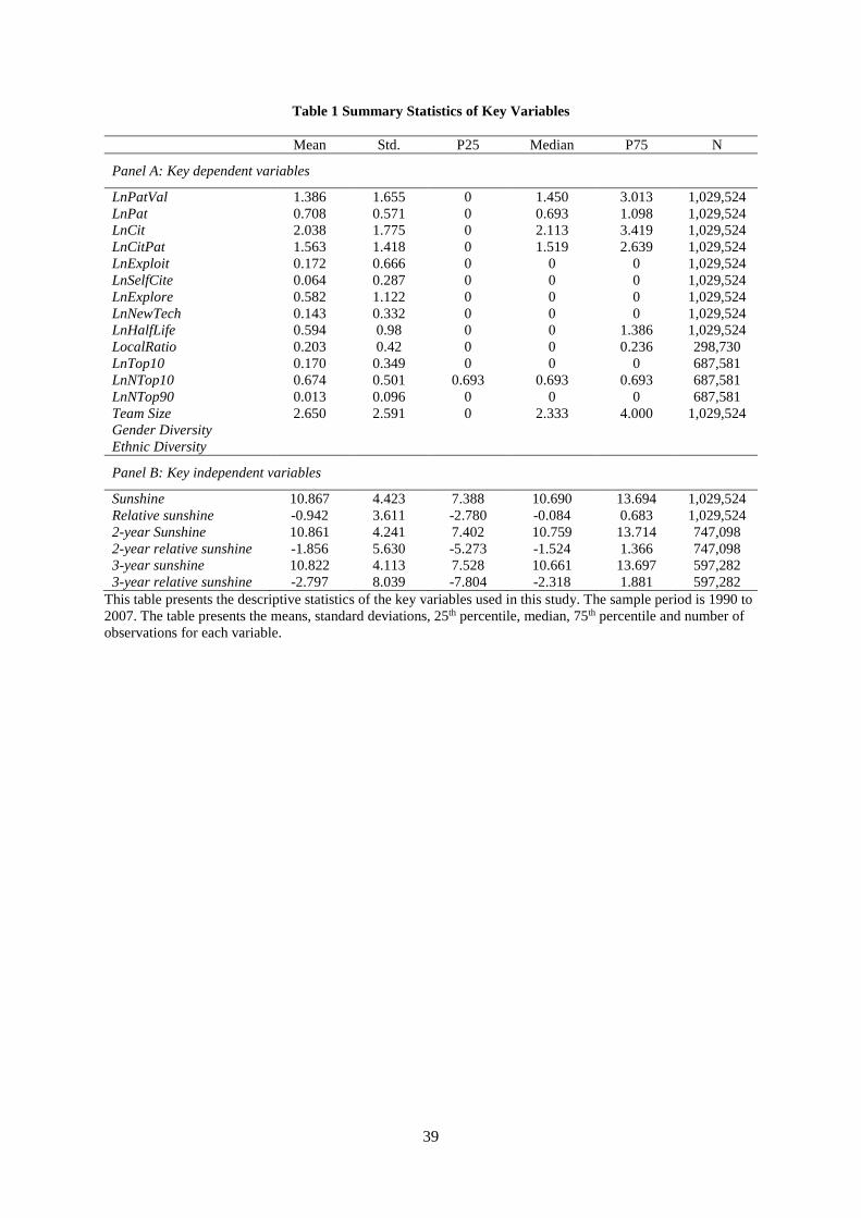
39

Table 1 Summary Statistics of Key Variables Mean Std. P25 Median P75 N

Panel A: Key dependent variables

LnPatVal 1.386 1.655 0 1.450 3.013 1,029,524 LnPat 0.708 0.571 0 0.693 1.098 1,029,524 LnCit 2.038 1.775 0 2.113 3.419 1,029,524 LnCitPat 1.563 1.418 0 1.519 2.639 1,029,524 LnExploit 0.172 0.666 0 0 0 1,029,524 LnSelfCite 0.064 0.287 0 0 0 1,029,524 LnExplore 0.582 1.122 0 0 0 1,029,524 LnNewTech 0.143 0.332 0 0 0 1,029,524 LnHalfLife 0.594 0.98 0 0 1.386 1,029,524 LocalRatio 0.203 0.42 0 0 0.236 298,730 LnTop10 0.170 0.349 0 0 0 687,581 LnNTop10 0.674 0.501 0.693 0.693 0.693 687,581 LnNTop90 0.013 0.096 0 0 0 687,581 Team Size 2.650 2.591 0 2.333 4.000 1,029,524 Gender Diversity Ethnic Diversity

Panel B: Key independent variables

Sunshine 10.867 4.423 7.388 10.690 13.694 1,029,524 Relative sunshine -0.942 3.611 -2.780 -0.084 0.683 1,029,524 2-year Sunshine 10.861 4.241 7.402 10.759 13.714 747,098 2-year relative sunshine -1.856 5.630 -5.273 -1.524 1.366 747,098 3-year sunshine 10.822 4.113 7.528 10.661 13.697 597,282 3-year relative sunshine -2.797 8.039 -7.804 -2.318 1.881 597,282

This table presents the descriptive statistics of the key variables used in this study. The sample period is 1990 to 2007. The table presents the means, standard deviations, 25th percentile, median, 75th percentile and number of observations for each variable.

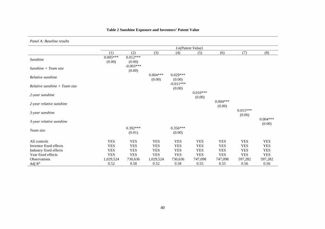
40

Table 2 Sunshine Exposure and Inventors’ Patent Value

Panel A: Baseline results

Ln(Patent Value) (1) (2) (3) (4) (5) (6) (7) (8)

Sunshine 0.005*** (0.00)

0.012*** (0.00)

Sunshine × Team size -0.003*** (0.00)

Relative sunshine 0.004*** (0.00)

0.029*** (0.00)

Relative sunshine × Team size -0.011*** (0.00)

2-year sunshine 0.010*** (0.00)

2-year relative sunshine 0.004*** (0.00)

3-year sunshine 0.015*** (0.00)

3-year relative sunshine 0.004*** (0.00)

Team size 0.392*** (0.01)

0.356*** (0.00)

All controls YES YES YES YES YES YES YES YES Inventor fixed effects YES YES YES YES YES YES YES YES Industry fixed effects YES YES YES YES YES YES YES YES Year fixed effects YES YES YES YES YES YES YES YES Observations 1,029,524 730,636 1,029,524 730,636 747,098 747,098 597,282 597,282 Adj R2 0.52 0.58 0.52 0.58 0.55 0.55 0.56 0.56

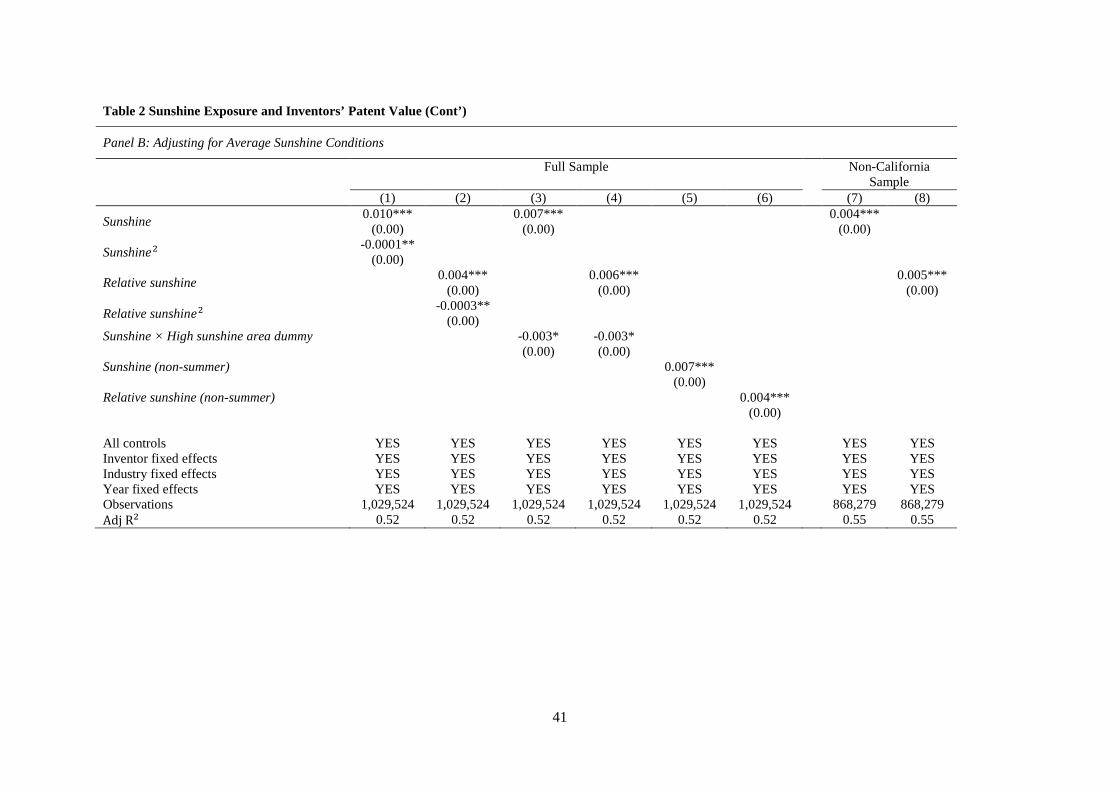
41

Table 2 Sunshine Exposure and Inventors’ Patent Value (Cont’)

Panel B: Adjusting for Average Sunshine Conditions

Full Sample Non-California Sample

(1) (2) (3) (4) (5) (6) (7) (8)

Sunshine 0.010*** (0.00)

0.007*** (0.00)

0.004*** (0.00)

Sunshin𝑒𝑒2 -0.0001** (0.00)

Relative sunshine 0.004*** (0.00)

0.006*** (0.00)

0.005*** (0.00)

Relative sunshin𝑒𝑒2 -0.0003** (0.00)

Sunshine × High sunshine area dummy -0.003* (0.00)

-0.003* (0.00)

Sunshine (non-summer) 0.007*** (0.00)

Relative sunshine (non-summer) 0.004*** (0.00)

All controls YES YES YES YES YES YES YES YES Inventor fixed effects YES YES YES YES YES YES YES YES Industry fixed effects YES YES YES YES YES YES YES YES Year fixed effects YES YES YES YES YES YES YES YES Observations 1,029,524 1,029,524 1,029,524 1,029,524 1,029,524 1,029,524 868,279 868,279 Adj R2 0.52 0.52 0.52 0.52 0.52 0.52 0.55 0.55

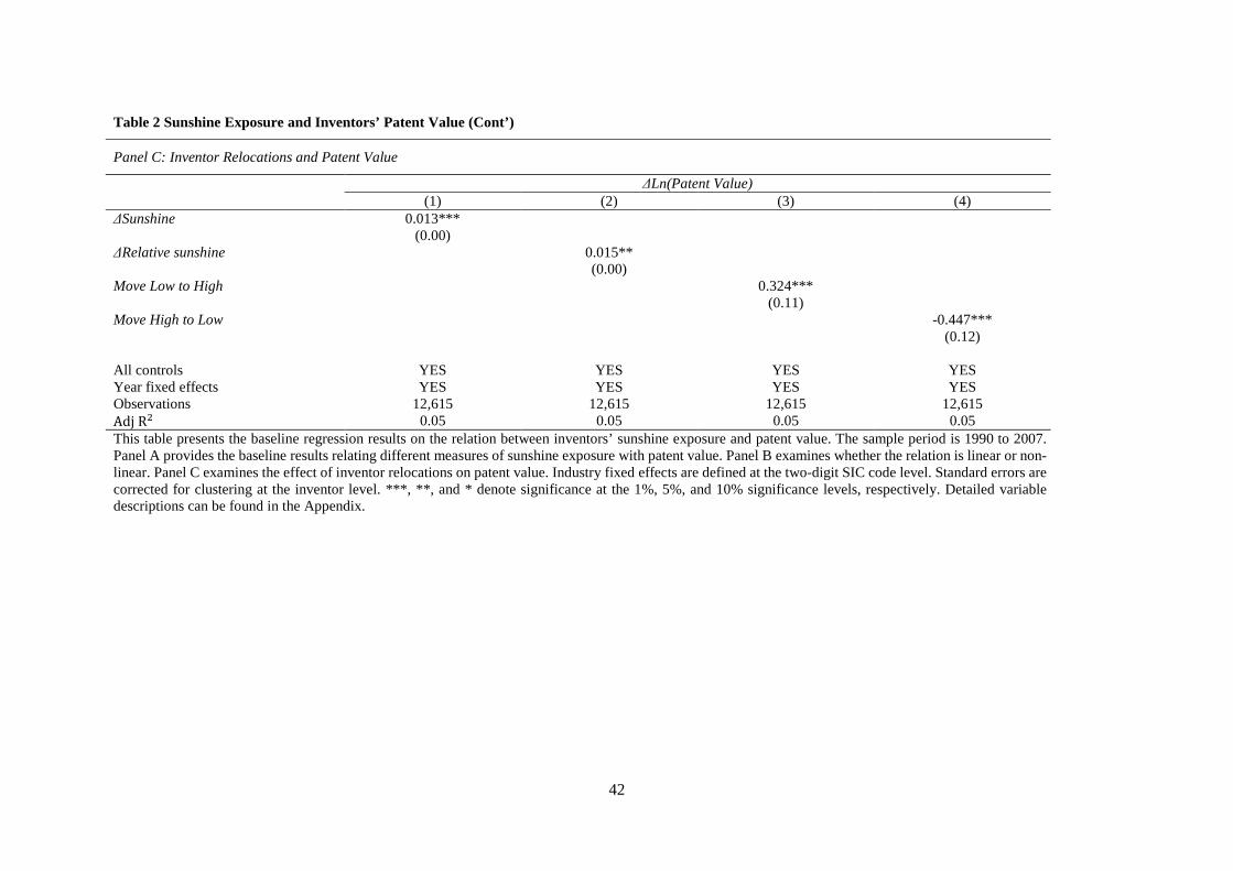
42

Table 2 Sunshine Exposure and Inventors’ Patent Value (Cont’)

Panel C: Inventor Relocations and Patent Value

ΔLn(Patent Value) (1) (2) (3) (4) ΔSunshine 0.013***

(0.00)

ΔRelative sunshine 0.015** (0.00)

Move Low to High 0.324*** (0.11)

Move High to Low -0.447*** (0.12)

All controls YES YES YES YES Year fixed effects YES YES YES YES Observations 12,615 12,615 12,615 12,615 Adj R2 0.05 0.05 0.05 0.05 This table presents the baseline regression results on the relation between inventors’ sunshine exposure and patent value. The sample period is 1990 to 2007. Panel A provides the baseline results relating different measures of sunshine exposure with patent value. Panel B examines whether the relation is linear or non-linear. Panel C examines the effect of inventor relocations on patent value. Industry fixed effects are defined at the two-digit SIC code level. Standard errors are corrected for clustering at the inventor level. ***, **, and * denote significance at the 1%, 5%, and 10% significance levels, respectively. Detailed variable descriptions can be found in the Appendix.

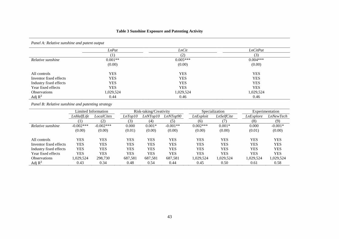
43

Table 3 Sunshine Exposure and Patenting Activity

Panel A: Relative sunshine and patent output

LnPat LnCit LnCitPat (1) (2) (3) Relative sunshine 0.001**

(0.00) 0.005***

(0.00) 0.004***

(0.00) All controls YES YES YES Inventor fixed effects YES YES YES Industry fixed effects YES YES YES Year fixed effects YES YES YES Observations 1,029,524 1,029,524 1,029,524 Adj R2 0.44 0.46 0.46

Panel B: Relative sunshine and patenting strategy

Limited Information Risk-taking/Creativity Specialization Experimentation LnHalfLife LocalCites LnTop10 LnNTop10 LnNTop90 LnExploit LnSelfCite LnExplore LnNewTech (1) (2) (3) (4) (5) (6) (7) (8) (9) Relative sunshine -0.002***

(0.00) -0.002***

(0.00) 0.000

(0.01) 0.001* (0.00)

-0.001** (0.00)

0.002*** (0.00)

0.001* (0.00)

0.000 (0.01)

-0.001* (0.00)

All controls YES YES YES YES YES YES YES YES YES Inventor fixed effects YES YES YES YES YES YES YES YES YES Industry fixed effects YES YES YES YES YES YES YES YES YES Year fixed effects YES YES YES YES YES YES YES YES YES Observations 1,029,524 298,730 687,581 687,581 687,581 1,029,524 1,029,524 1,029,524 1,029,524 Adj R2 0.43 0.34 0.48 0.54 0.44 0.45 0.50 0.61 0.58

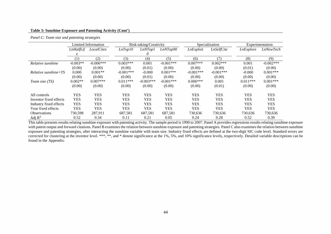
44

Table 3: Sunshine Exposure and Patenting Activity (Cont’)

Panel C: Team size and patenting strategies

Limited Information Risk-taking/Creativity Specialization Experimentation LnHalfLif

e LocalCites LnTop10 LnNTop1

0 LnNTop90 LnExploit LnSelfCite LnExplore LnNewTech

(1) (2) (3) (4) (5) (6) (7) (8) (9) Relative sunshine -0.003**

(0.00) -0.006***

(0.00) 0.003***

(0.00) 0.001 (0.01)

-0.001*** (0.00)

0.007*** (0.00)

0.002*** (0.00)

0.001 (0.01)

-0.002*** (0.00)

Relative sunshine×TS 0.000 (0.00)

0.001** (0.00)

-0.001*** (0.00)

-0.000 (0.01)

0.001*** (0.00)

-0.001*** (0.00)

-0.001*** (0.00)

-0.000 (0.00)

0.001*** (0.00)

Team size (TS) 0.002** (0.00)

0.007*** (0.00)

0.011*** (0.00)

-0.003*** (0.00)

-0.001*** (0.00)

0.006*** (0.00)

0.001 (0.01)

0.011*** (0.00)

0.001*** (0.00)

All controls YES YES YES YES YES YES YES YES YES Inventor fixed effects YES YES YES YES YES YES YES YES YES Industry fixed effects YES YES YES YES YES YES YES YES YES Year fixed effects YES YES YES YES YES YES YES YES YES Observations 730,598 287,911 687,581 687,581 687,581 730,636 730,636 730,636 730,636 Adj R2 0.52 0.34 0.11 0.21 0.05 0.24 0.28 0.52 0.39

This table presents results relating sunshine exposure with patenting activity. The sample period is 1990 to 2007. Panel A provides regressions results relating sunshine exposure with patent output and forward citations. Panel B examines the relation between sunshine exposure and patenting strategies. Panel C also examines the relation between sunshine exposure and patenting strategies, after interacting the sunshine variable with team size. Industry fixed effects are defined at the two-digit SIC code level. Standard errors are corrected for clustering at the inventor level. ***, **, and * denote significance at the 1%, 5%, and 10% significance levels, respectively. Detailed variable descriptions can be found in the Appendix.

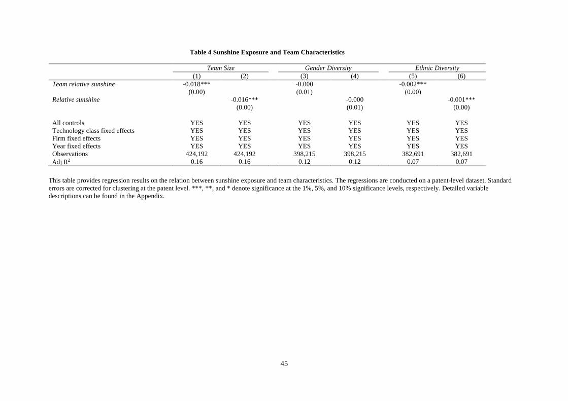
45

Table 4 Sunshine Exposure and Team Characteristics Team Size Gender Diversity Ethnic Diversity (1) (2) (3) (4) (5) (6) Team relative sunshine -0.018***

(0.00) -0.000

(0.01) -0.002***

(0.00)

Relative sunshine -0.016*** (0.00)

-0.000 (0.01)

-0.001*** (0.00)

All controls YES YES YES YES YES YES Technology class fixed effects YES YES YES YES YES YES Firm fixed effects YES YES YES YES YES YES Year fixed effects YES YES YES YES YES YES Observations 424,192 424,192 398,215 398,215 382,691 382,691 Adj R2 0.16 0.16 0.12 0.12 0.07 0.07

This table provides regression results on the relation between sunshine exposure and team characteristics. The regressions are conducted on a patent-level dataset. Standard errors are corrected for clustering at the patent level. ***, **, and * denote significance at the 1%, 5%, and 10% significance levels, respectively. Detailed variable descriptions can be found in the Appendix.

46

Table 5 Sunshine Exposure and Managerial Decisions

Panel A: Sunshine around firm’s headquarters

SG&A/Assets Employee Treatment R&D/Assets PPE/Assets (1) (2) (3) (4) (5) (6) (7) (8)

HQ Sunshine -0.000 (0.01)

0.000 (0.01)

0.000 (0.00)

0.000 (0.01)

HQ Sunshine × Dispersion 0.000 (0.01)

-0.000 (0.00)

-0.000 (0.00)

-0.000 (0.01)

HQ Relative sunshine 0.000 (0.01)

-0.003 (0.01)

0.000 (0.01)

0.000 (0.00)

HQ Relative sunshine × Dispersion -0.000 (0.01)

0.000 (0.00)

-0.001 (0.00)

-0.000 (0.00)

Dispersion -0.001 (0.01)

-0.000 (0.01)

0.002 (0.01)

0.000 (0.00)

0.001* (0.00)

0.000 (0.01)

0.001 (0.01)

0.000 (0.00)

All controls YES YES YES YES YES YES YES YES Firm fixed effects YES YES YES YES YES YES YES YES Year fixed effects YES YES YES YES YES YES YES YES Observations 10,131 10,131 4,063 4,063 11,536 11,536 11,536 11,536 Adj R2 0.81 0.81 0.56 0.56 0.82 0.82 0.89 0.89

Panel B: Sunshine around firm’s division location

SG&A/Assets Employee Treatment R&D/Assets PPE/Assets (1) (2) (3) (4) (5) (6) (7) (8)

Division sunshine -0.001 (0.01)

-0.001 (0.01)

0.000 (0.01)

-0.000 (0.01)

Division relative sunshine -0.001 (0.01)

0.005 (0.01)

-0.001 (0.01)

0.001 (0.01)

All controls YES YES YES YES YES YES YES YES Firm fixed effects YES YES YES YES YES YES YES YES Year fixed effects YES YES YES YES YES YES YES YES Observations 11,306 11,306 4,720 4,720 12,981 12,981 12,981 12,981 Adj R2 0.81 0.81 0.54 0.54 0.63 0.63 0.89 0.89

47

Table 5: Sunshine Exposure and Managerial Decisions (Cont’)

Panel C: Sub-sample of geographically dispersed firms

SG&A/Assets Employee Treatment R&D/Assets PPE/Assets (1) (2) (3) (4) (5) (6) (7) (8) HQ Sunshine -0.001

(0.01) -0.002

(0.01) -0.000

(0.00) -0.000

(0.01)

Division sunshine -0.002 (0.01)

0.003 (0.01)

-0.000 (0.01)

-0.000 (0.01)

HQ Relative sunshine -0.001 (0.01)

-0.002 (0.01)

-0.000 (0.01)

-0.000 (0.01)

Division relative sunshine 0.002 (0.01)

0.016 (0.01)

-0.002 (0.01)

0.000 (0.01)

All controls YES YES YES YES YES YES YES YES Firm fixed effects YES YES YES YES YES YES YES YES Year fixed effects YES YES YES YES YES YES YES YES Observations 4,508 4,508 1,932 1,932 4,993 4,993 4,993 4,993 Adj R2 0.83 0.83 0.56 0.56 0.78 0.78 0.91 0.91

This table provides regression results on the relation between firm-level sunshine exposure and key corporate strategies which have the ability to influence patenting activity. The sample period is 1990 to 2007. The regressions are conducted on a firm-level dataset. Panel A relates sunshine around a firm’s headquarters’ location and corporate strategies. Panel B relates average sunshine around firms’ divisions and corporate strategies. Panel C examines a sub-sample of geographically dispersed firms. Standard errors are corrected for clustering at the firm level. ***, **, and * denote significance at the 1%, 5%, and 10% significance levels, respectively. Detailed variable descriptions can be found in the Appendix.

48

Table 6 Sunshine Exposure and Local Spillovers

Panel A: Sunshine and migration trends

Overall Migration Inventor Migration Net migration Net migration/Population Ln(Number of Inventors) (1) (2) (3) (4) (5) (6) Sunshine 0.054

(0.05) 0.001

(0.01) -0.001

(0.01)

Relative sunshine -0.005 (0.08)

-0.001 (0.01)

-0.002 (0.01)

Ln (Median income) 15.130*** (1.94)

14.955*** (2.01)

0.147*** (0.02)

0.147*** (0.02)

0.497*** (0.19)

0.497*** (0.19)

State fixed effects YES YES YES YES NO NO County fixed effects NO NO NO NO YES YES Year fixed effects NO NO NO NO YES YES Observations 729 729 729 729 19,656 19,656 Adj R2 0.35 0.35 0.39 0.39 0.95 0.95

Panel B: Sunshine exposure and use of local information set

Ln(Local citations) Local Citations/Patent (1) (2) (3) (4) Sunshine -0.005***

(0.00) -0.055***

(0.00)

Relative sunshine -0.002* (0.00)

-0.045*** (0.00)

All controls YES YES YES YES Inventor fixed effects YES YES YES YES Industry fixed effects YES YES YES YES Year fixed effects YES YES YES YES Observations 732,081 732,081 732,081 732,081 Adj R2 0.46 0.46 0.42 0.42

This table presents the regression results on the effects of local spillovers. Panel A examines the relation between sunshine conditions and local net migration. Overall migrations utilizes county level data on the net migration figures over a ten year period and relates this figure with average sunshine and relative sunshine conditions over a ten year period. The results in columns (1) to (4) are based on a cross-sectional regression. Inventor migration utilized data from the patent data on inventor relocations, and related sunshine conditions in each county-year with net inventor migration in each county-year. In Panel A standard errors are corrected for clustering at the county level. Panel B examines the relation between sunshine conditions and the reliance of inventors on local knowledge. These regressions are conducted on the inventor-level dataset. Standard errors in Panel B are corrected for clustering at the inventor level. ***, **, and * denote significance at the 1%, 5%, and 10% significance levels, respectively. Detailed variable descriptions can be found in the Appendix.

49

Table 7 Sunshine Exposure and Local Economic Performance

County Level Analysis State Level Analysis Ln(Per-Capita Inc.) Ln(Local Sales) Ln(Real GDP) Ln(Income Tax) (1) (2) (3) (4) (5) (6) (7) (8)

Sunshine -0.001 (0.01)

0.015 (0.01)

-0.003* (0.00)

-0.001 (0.01)

Relative sunshine -0.001 (0.01)

-0.004 (0.02)

-0.001 (0.01)

-0.001 (0.01)

County fixed effects YES YES YES YES NO NO NO NO State fixed effects NO NO NO NO YES YES YES YES Year fixed effects YES YES YES YES YES YES YES YES Observations 4,830 4,830 4,830 4,830 822 822 580 580 Adj R2 0.98 0.98 0.87 0.87 0.99 0.99 0.99 0.98

This table presents regression results on the relation between local sunshine conditions and economic performance. The results presented in columns (1) to (4) are based on county-level economic data, while the results presented in columns (5) to (8) are based on state-level economic data. Standard errors in columns (1) to (4) are corrected for clustering at the county level, while standard errors in columns (5) to (8) are corrected for clustering at the state level. ***, **, and * denote significance at the 1%, 5%, and 10% significance levels, respectively. Detailed variable descriptions can be found in the Appendix.

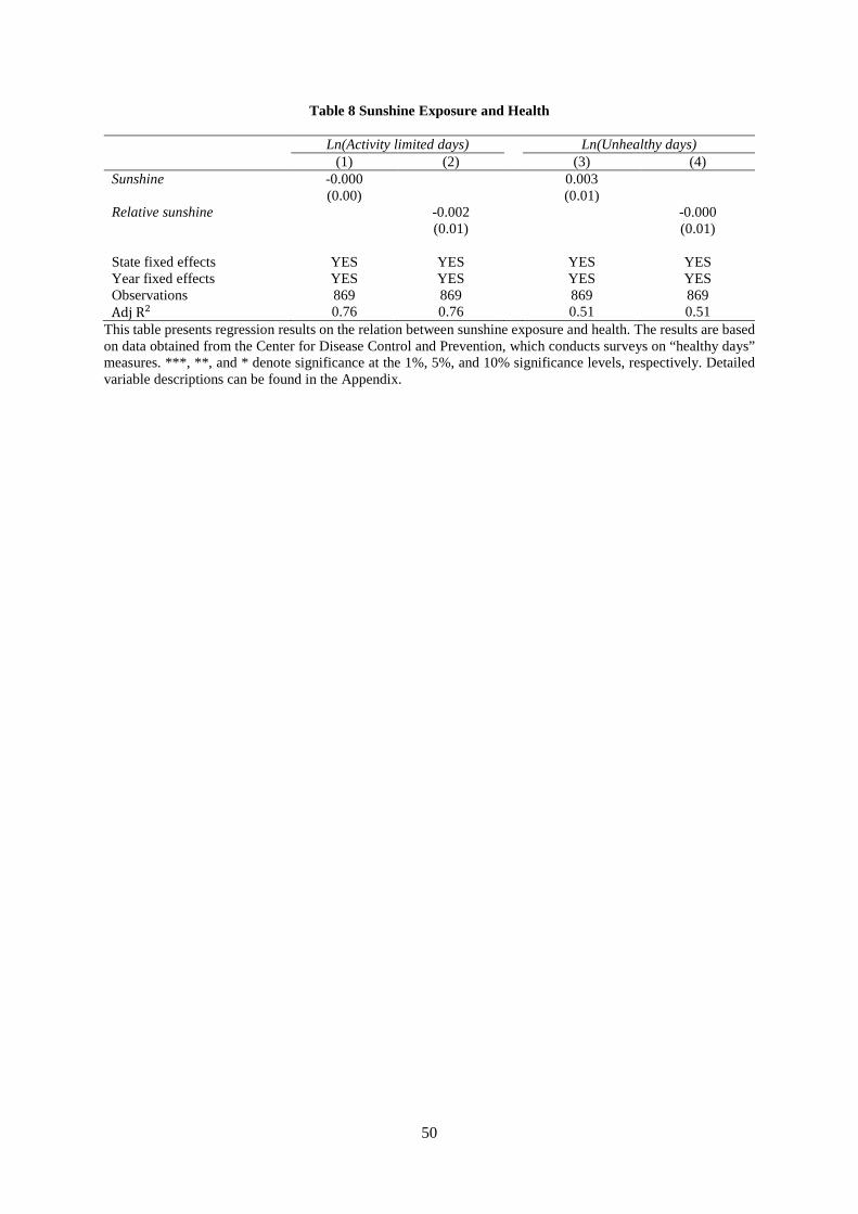
50

Table 8 Sunshine Exposure and Health

Ln(Activity limited days) Ln(Unhealthy days) (1) (2) (3) (4)

Sunshine -0.000 (0.00)

0.003 (0.01)

Relative sunshine -0.002 (0.01)

-0.000 (0.01)

State fixed effects YES YES YES YES Year fixed effects YES YES YES YES Observations 869 869 869 869 Adj R2 0.76 0.76 0.51 0.51

This table presents regression results on the relation between sunshine exposure and health. The results are based on data obtained from the Center for Disease Control and Prevention, which conducts surveys on “healthy days” measures. ***, **, and * denote significance at the 1%, 5%, and 10% significance levels, respectively. Detailed variable descriptions can be found in the Appendix.

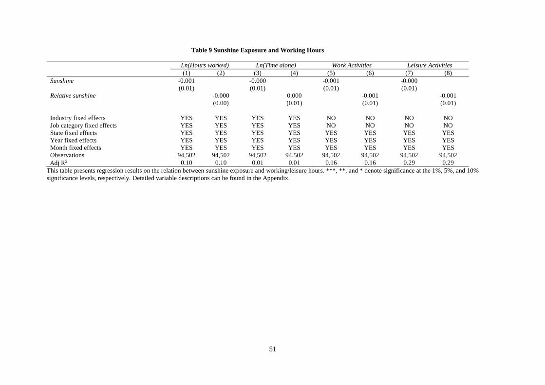
51

Table 9 Sunshine Exposure and Working Hours Ln(Hours worked) Ln(Time alone) Work Activities Leisure Activities (1) (2) (3) (4) (5) (6) (7) (8) Sunshine -0.001

(0.01) -0.000

(0.01) -0.001

(0.01) -0.000

(0.01)

Relative sunshine -0.000 (0.00)

0.000 (0.01)

-0.001 (0.01)

-0.001 (0.01)

Industry fixed effects YES YES YES YES NO NO NO NO Job category fixed effects YES YES YES YES NO NO NO NO State fixed effects YES YES YES YES YES YES YES YES Year fixed effects YES YES YES YES YES YES YES YES Month fixed effects YES YES YES YES YES YES YES YES Observations 94,502 94,502 94,502 94,502 94,502 94,502 94,502 94,502 Adj R2 0.10 0.10 0.01 0.01 0.16 0.16 0.29 0.29

This table presents regression results on the relation between sunshine exposure and working/leisure hours. ***, **, and * denote significance at the 1%, 5%, and 10% significance levels, respectively. Detailed variable descriptions can be found in the Appendix.

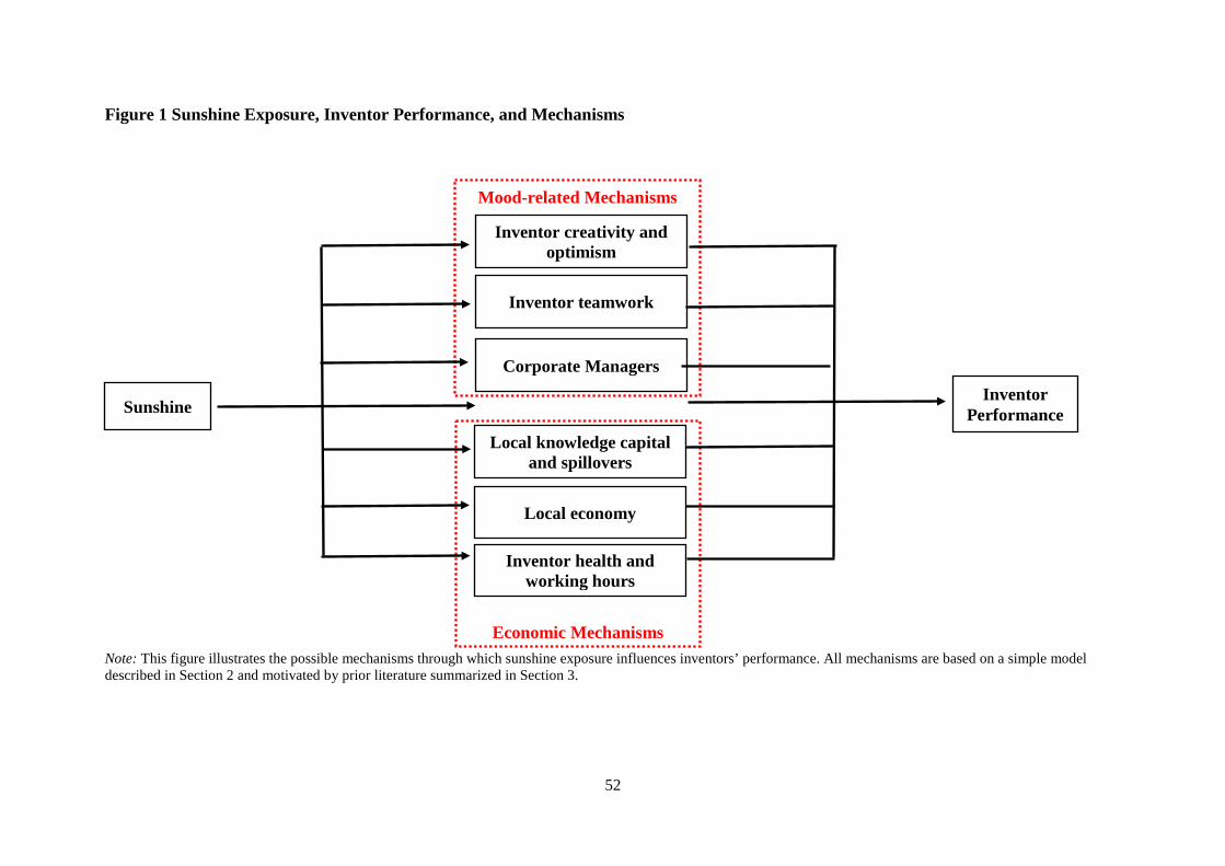
52

Figure 1 Sunshine Exposure, Inventor Performance, and Mechanisms

Note: This figure illustrates the possible mechanisms through which sunshine exposure influences inventors’ performance. All mechanisms are based on a simple model described in Section 2 and motivated by prior literature summarized in Section 3.

Inventor creativity and optimism

Inventor Performance Sunshine

Inventor teamwork

Corporate Managers

Local knowledge capital and spillovers

Local economy

Inventor health and working hours

Mood-related Mechanisms

Economic Mechanisms

53

In the Mood for Creativity: Weather-induced Mood, Inventor Productivity, and Firm Value

ONLINE APPENDIX

54

This online appendix reports additional tests referred to in the paper. Table OA.1

provides descriptive statics for our sunshine variables across states. An important question to

ask is whether annual sky cover varies sufficiently, both across time and locations, to be able

to influence innovation outcomes in an economically significant way. Table OA.1 reveals that

states differ significantly in terms of their average sunshine. For example, Alaska only has

roughly 5.80 sunny days per month, while Wyoming has roughly 19.25 sunny days per month.

Although we would expect that some states are sunnier than others, this assumption raises a

potential selection problem; for example, better quality inventors might flock to states with

more sunshine. To address this potential problem, we concentrate on relative sunshine in our

main analysis, which captures the unexpected level of sunshine.

[Insert Table OA.1 about here]

Table OA.2 reports the robustness tests for our baseline results reported in Table 2 of the

paper. In Panel A, we report baseline results for the full sample of inventors in the patent

database (ie. inventors who are both employed by publically listed firms and those that are not).

Since the primary dependent variable in Table 2, namely patent value (PatVal), is calculated

by observing the stock price reaction to patent grants, this measure of patent quality is not

available to us when examining inventors who are not employed by publically listed firms. As

such, in Panel A we use patent count (Pat), forward citations (Cit), and citations-per-patent

(CitPat) as the dependent variables. In addition, we cannot control for any firm-level

characteristics in our analysis, since this information is unavailable for inventors not employed

by publically listed firms. The model specification is therefore limited to regressing patent

output variables on sunshine exposure as well as inventor and year fixed effects. The results in

Panel A reveal a positive association between sunshine exposure and inventor’s patent output.

In Panel B, we examine the sub-sample of inventors that are not employed by publically

listed firms. We use the same empirical set-up as for the results reported in Panel A, and also

find a positive association between sunshine exposure and inventor productivity.

In Panel C, we exclude inventor-year observations from our sample where inventors do

not apply for any patents. In our baseline analysis, we follow common practice and replace

such “missing” years with zeros. We find that our results stay qualitatively unchanged in Panel

C.

In Panel D, we address the non-uniformity of inventors distributed geographically by

excluding from the sample all inventors who have ever resided in the rust belt states

(Pennsylvania, West Virginia, Ohio, Indiana, Michigan, Illinois, Iowa, and Wisconsin). It is

possible that our results are somehow contaminated by inventors moving away from rust belt

55

states and older industries to the west. We find consistent results. To address a similar concern,

in Panel E, we exclude from our sample those inventors that reside in California, Massachusetts,

and New York which are unusually innovative states. Finally, in Panel F we exclude from our

sample those inventors that have ever changed locations. This test helps us ensure that the

results are not driven by inventors relocating to more sunny areas (ie. California). The results

stay qualitatively unchanged.

In Panel G, we remove inventors from our sample that reside in close proximity to the

firm’s headquarters. In columns (1) and (2) we remove inventors that reside in the same county

as the firm is headquartered, while in columns (3) and (4) we remove inventors who reside in

the same state. Again, we find that the results stay qualitatively unchanged.

Finally, in Panel H we replace inventor fixed effects with firm fixed effects. This test

allows us to examine how inventors residing in different locations but employed by the same

firm react to changes in weather. Once again, we report a positive and significant association

between sunshine exposure and inventor productivity.

[Insert Table OA.2 about here]

In Table OA.3, we examine the characteristics of exploitative and exploratory patents.

Specifically, we utilize our patent-level dataset and run a linear probability model to examine

whether exploitative and exploratory patents are more or less likely to be “hits” or “flops”. We

include technology, firm, and year fixed effects in our regressions. We find that exploitative

patents are more likely to be “hits”, whereas exploratory patents are less likely to be “hits” and

more likely to be of “average” quality. In addition, we run an OLS model in which we regress

forward citations on exploitative and exploratory patents and find that exploitative patents

generate more forward citations while exploratory patents generate fewer forward citations.

Our results highlight that exploitative patents, while by definition not being as path-breaking

and “emergenative” as exploratory patents, cannot be considered as lower quality. In fact, by

all objective standards, it appears that exploitative patents are higher quality (on average)

compared with exploratory patents.

[Insert Table OA.3 about here]

In OA.4 we provide additional results on the effects that team dynamics have on inventor

productivity. Specifically, limiting the inventor-level sample to only those inventors that

produce at least one patent in a team, and relating team sunshine and team relative sunshine

with patent value, we find a weak positive relation for team sunshine and no relation for team

relative sunshine. In addition, we construct an indicator variable equal to one for inventor-year

observations where all co-inventors working on a patent have positive abnormal sunshine. We

56

find that inventor productivity is higher when his/her team members are affected by positive

weather, compared with when co-inventors are not similarly affected by good mood. Overall,

our result suggest that sunshine has a limited influence on inventor productivity via its effect

on teamwork. However, this does not appear to be the primary channel through which sunshine

affects productivity, with the effect appearing to be strongest for inventors working alone.

[Insert Table OA.4 about here]

Finally, in Table OA.5 we examine the effect that patent attorneys and patent examiners

have on the review process. Specifically, sunshine may improve the mood of patent attorneys,

who represent their client firms in preparing, filing, and prosecuting patent applications to

USPTO. Although patent attorneys cannot plausibly influence patent quality directly, sunshine

exposure might make them more efficient in developing the patent application from a legal

standpoint, with a higher quality patent application being less likely to be sent back due to

incomplete information and easier to process. As a consequence, the patent might be approved

faster, resulting in the technology being patented and brought to the market sooner.

In addition to patent attorneys, sunshine could also improve the mood of outside parties

in the patenting process. Patent examiners are employees of the USPTO who review patent

applications to determine whether the invention in each of the applications should be granted

a patent or not. Since the work of patent examiners involves certain extent of subjective

judgments, mood-induced behavioral traits of patent examiners may affect firm patenting

success. For example, when patent examiners are in good mood, they are more optimistic and

may have an upward bias in the subjective judgment of the quality of the patent application.

As a result, they are more likely to approve patent applications that are across-the-border,

which leads to greater firm patent output.

In Table OA.5, we examine whether sunshine conditions have the ability to influence the

patent review process or the efficiency of patent attorneys. The logic behind these tests is that

while patent reviewers and patent lawyers have little impact on the quality of inventions, they

do have the ability to slow down, or speed up the time it takes before a patent is granted. For

patent reviewers, we examine whether sunshine around the USPTO during the patent review

time has an effect on the review length of a patent. For each patent, we measure time under

review, as the time between patent application and patent granting. In Panel A, we relate time

under review with sunshine conditions around the USPTO during the review time.36F

36 We

36 For every patent, we measure the average sunshine exposure during the time when the patent is under review, since this is the time when sunshine exposure has the ability to influence patent reviewers. Towards this end, we

57

control for all firm level variables pertaining to the firm the patent is assigned to, and include

technology class, firm, and year fixed effects. We find that the coefficient estimate on both

sunshine variables are negative and significant, meaning that during sunnier periods, patent

office workers conduct their duties more efficiently, thus reducing the patent review time.

In Panel B, we relate time under review with sunshine conditions around the headquarters

during the review time. Although we have no way of knowing for sure, we assume that patent

lawyers work in the firm’s headquarters.37F

37 We also assume that patent lawyers can only have

an effect on the patent’s quality immediately prior to application, since this is when they will

be preparing the patent application. Sunshine exposure might make them more efficient in

developing the patent application from a legal standpoint, with a higher quality patent

application being less likely to be sent back due to incomplete information and easier to process.

The results reported in Panel B show that sunshine conditions around the firm’s headquarter

location in the month preceding the patent application has no effect on time under review. We

conclude that patent lawyers play a limited role in developing patent applications, or that their

work has little impact on how quickly the patent is assessed. In Panel C, we examine whether

the positive association between inventor sunshine exposure and patent value holds, even after

controlling for patent review time. Using the inventor-level sample in which we calculate the

average review time for the patents applied for in a given year, we find that the positive

association between inventor sunshine exposure and patent value holds, even though the

relation between review time and patent value is highly positive and significant. Another

important implication is that although sunshine around USPTO results in patent reviewers

working more efficiently, this factor does not explain the positive association between the

sunshine conditions of inventors and their improved productivity.

[Insert Table OA.5 about here]

measure the sunshine conditions within a 50-kilomemeter radius of the location of the USPTO in Alexandria, Virginia. 37 For patent attorneys, we measure the sunshine exposure within a 50-killometer radius of the firm’s headquarters during the month preceding the patent application.

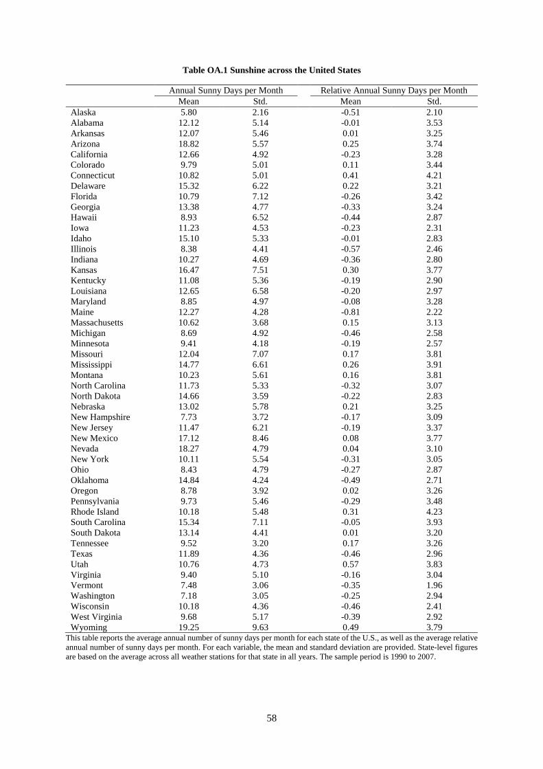
58

Table OA.1 Sunshine across the United States Annual Sunny Days per Month Relative Annual Sunny Days per Month Mean Std. Mean Std. Alaska 5.80 2.16 -0.51 2.10 Alabama 12.12 5.14 -0.01 3.53 Arkansas 12.07 5.46 0.01 3.25 Arizona 18.82 5.57 0.25 3.74 California 12.66 4.92 -0.23 3.28 Colorado 9.79 5.01 0.11 3.44 Connecticut 10.82 5.01 0.41 4.21 Delaware 15.32 6.22 0.22 3.21 Florida 10.79 7.12 -0.26 3.42 Georgia 13.38 4.77 -0.33 3.24 Hawaii 8.93 6.52 -0.44 2.87 Iowa 11.23 4.53 -0.23 2.31 Idaho 15.10 5.33 -0.01 2.83 Illinois 8.38 4.41 -0.57 2.46 Indiana 10.27 4.69 -0.36 2.80 Kansas 16.47 7.51 0.30 3.77 Kentucky 11.08 5.36 -0.19 2.90 Louisiana 12.65 6.58 -0.20 2.97 Maryland 8.85 4.97 -0.08 3.28 Maine 12.27 4.28 -0.81 2.22 Massachusetts 10.62 3.68 0.15 3.13 Michigan 8.69 4.92 -0.46 2.58 Minnesota 9.41 4.18 -0.19 2.57 Missouri 12.04 7.07 0.17 3.81 Mississippi 14.77 6.61 0.26 3.91 Montana 10.23 5.61 0.16 3.81 North Carolina 11.73 5.33 -0.32 3.07 North Dakota 14.66 3.59 -0.22 2.83 Nebraska 13.02 5.78 0.21 3.25 New Hampshire 7.73 3.72 -0.17 3.09 New Jersey 11.47 6.21 -0.19 3.37 New Mexico 17.12 8.46 0.08 3.77 Nevada 18.27 4.79 0.04 3.10 New York 10.11 5.54 -0.31 3.05 Ohio 8.43 4.79 -0.27 2.87 Oklahoma 14.84 4.24 -0.49 2.71 Oregon 8.78 3.92 0.02 3.26 Pennsylvania 9.73 5.46 -0.29 3.48 Rhode Island 10.18 5.48 0.31 4.23 South Carolina 15.34 7.11 -0.05 3.93 South Dakota 13.14 4.41 0.01 3.20 Tennessee 9.52 3.20 0.17 3.26 Texas 11.89 4.36 -0.46 2.96 Utah 10.76 4.73 0.57 3.83 Virginia 9.40 5.10 -0.16 3.04 Vermont 7.48 3.06 -0.35 1.96 Washington 7.18 3.05 -0.25 2.94 Wisconsin 10.18 4.36 -0.46 2.41 West Virginia 9.68 5.17 -0.39 2.92 Wyoming 19.25 9.63 0.49 3.79

This table reports the average annual number of sunny days per month for each state of the U.S., as well as the average relative annual number of sunny days per month. For each variable, the mean and standard deviation are provided. State-level figures are based on the average across all weather stations for that state in all years. The sample period is 1990 to 2007.

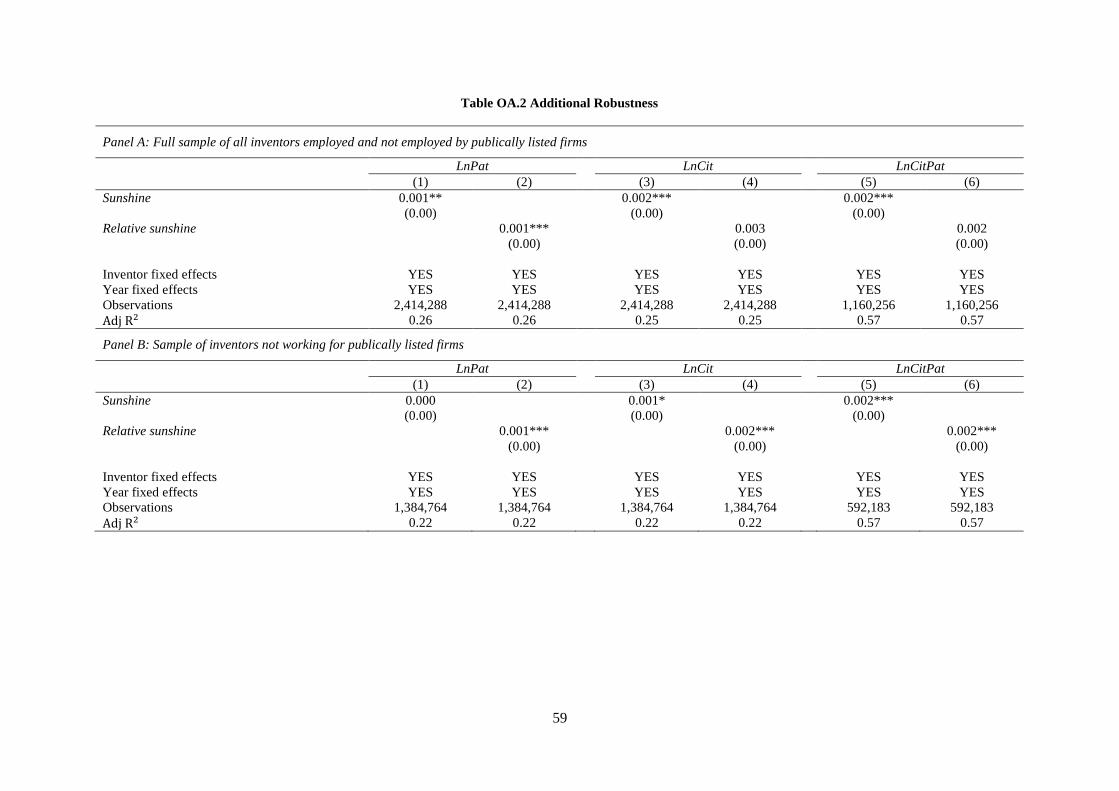
59

Table OA.2 Additional Robustness

Panel A: Full sample of all inventors employed and not employed by publically listed firms

LnPat LnCit LnCitPat (1) (2) (3) (4) (5) (6)

Sunshine 0.001** (0.00)

0.002*** (0.00)

0.002*** (0.00)

Relative sunshine 0.001*** (0.00)

0.003 (0.00)

0.002 (0.00)

Inventor fixed effects YES YES YES YES YES YES Year fixed effects YES YES YES YES YES YES Observations 2,414,288 2,414,288 2,414,288 2,414,288 1,160,256 1,160,256 Adj R2 0.26 0.26 0.25 0.25 0.57 0.57

Panel B: Sample of inventors not working for publically listed firms

LnPat LnCit LnCitPat (1) (2) (3) (4) (5) (6)

Sunshine 0.000 (0.00)

0.001* (0.00)

0.002*** (0.00)

Relative sunshine 0.001*** (0.00)

0.002*** (0.00)

0.002*** (0.00)

Inventor fixed effects YES YES YES YES YES YES Year fixed effects YES YES YES YES YES YES Observations 1,384,764 1,384,764 1,384,764 1,384,764 592,183 592,183 Adj R2 0.22 0.22 0.22 0.22 0.57 0.57

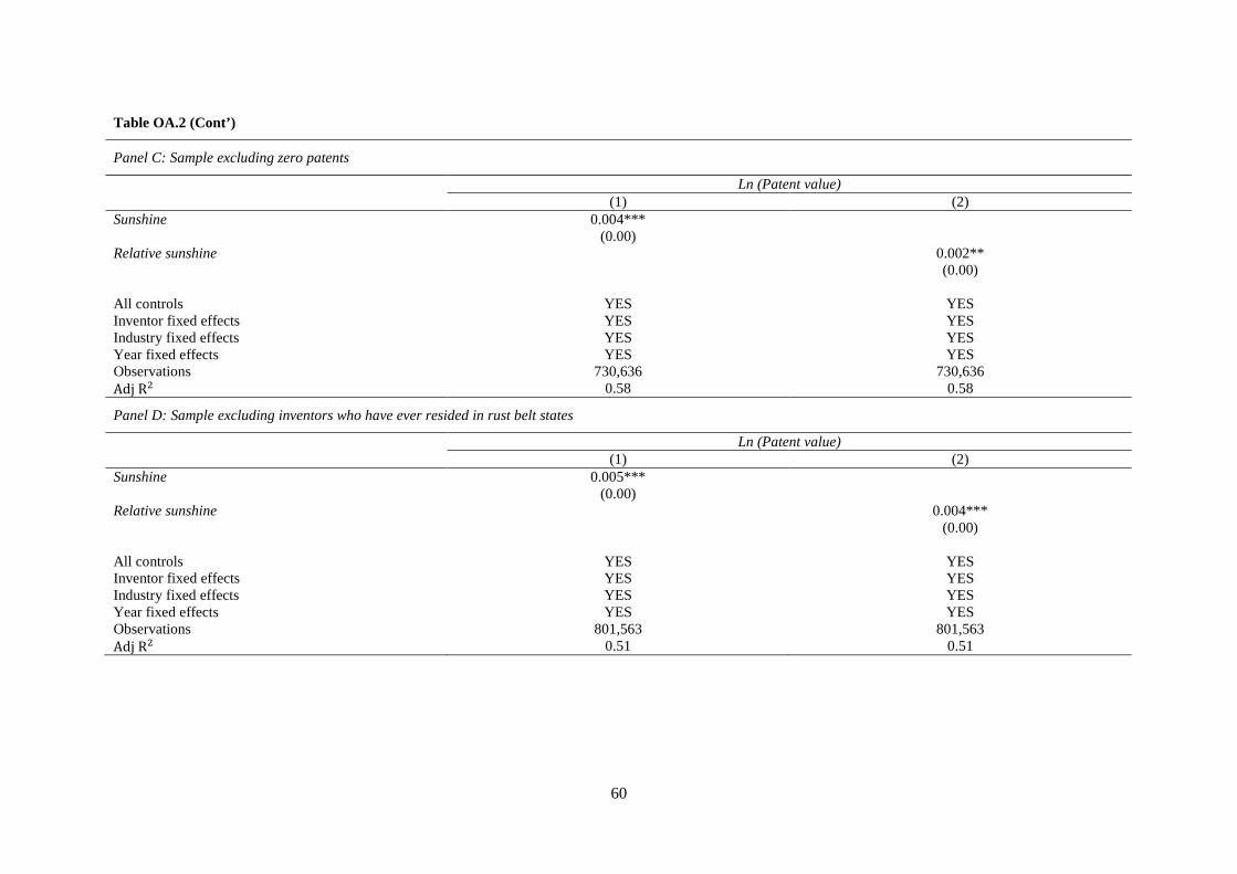
60

Table OA.2 (Cont’)

Panel C: Sample excluding zero patents

Ln (Patent value) (1) (2)

Sunshine 0.004*** (0.00)

Relative sunshine 0.002** (0.00)

All controls YES YES Inventor fixed effects YES YES Industry fixed effects YES YES Year fixed effects YES YES Observations 730,636 730,636 Adj R2 0.58 0.58

Panel D: Sample excluding inventors who have ever resided in rust belt states

Ln (Patent value) (1) (2)

Sunshine 0.005*** (0.00)

Relative sunshine 0.004*** (0.00)

All controls YES YES Inventor fixed effects YES YES Industry fixed effects YES YES Year fixed effects YES YES Observations 801,563 801,563 Adj R2 0.51 0.51

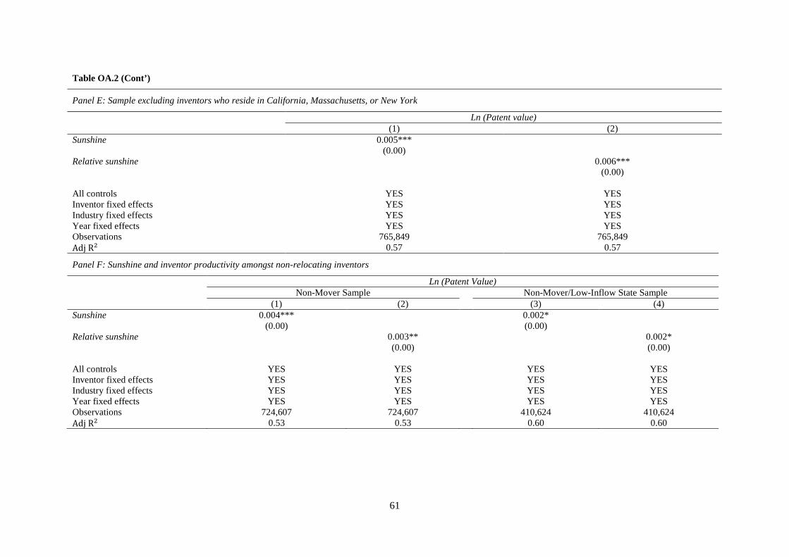
61

Table OA.2 (Cont’)

Panel E: Sample excluding inventors who reside in California, Massachusetts, or New York

Ln (Patent value) (1) (2)

Sunshine 0.005*** (0.00)

Relative sunshine 0.006*** (0.00)

All controls YES YES Inventor fixed effects YES YES Industry fixed effects YES YES Year fixed effects YES YES Observations 765,849 765,849 Adj R2 0.57 0.57

Panel F: Sunshine and inventor productivity amongst non-relocating inventors

Ln (Patent Value) Non-Mover Sample Non-Mover/Low-Inflow State Sample (1) (2) (3) (4) Sunshine 0.004***

(0.00) 0.002*

(0.00)

Relative sunshine 0.003** (0.00)

0.002* (0.00)

All controls YES YES YES YES Inventor fixed effects YES YES YES YES Industry fixed effects YES YES YES YES Year fixed effects YES YES YES YES Observations 724,607 724,607 410,624 410,624 Adj R2 0.53 0.53 0.60 0.60

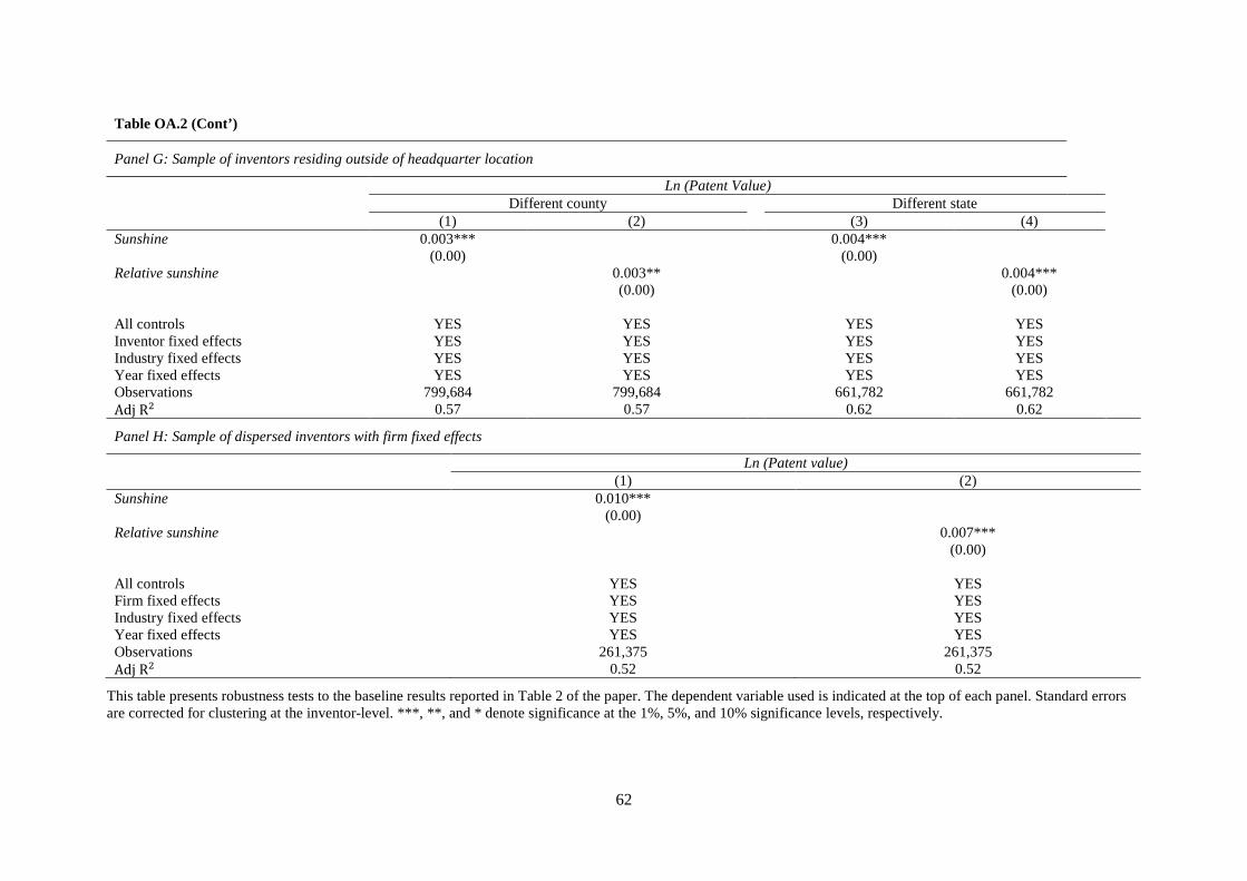
62

Table OA.2 (Cont’)

Panel G: Sample of inventors residing outside of headquarter location

Ln (Patent Value) Different county Different state (1) (2) (3) (4)

Sunshine 0.003*** (0.00)

0.004*** (0.00)

Relative sunshine 0.003** (0.00)

0.004*** (0.00)

All controls YES YES YES YES Inventor fixed effects YES YES YES YES Industry fixed effects YES YES YES YES Year fixed effects YES YES YES YES Observations 799,684 799,684 661,782 661,782 Adj R2 0.57 0.57 0.62 0.62

Panel H: Sample of dispersed inventors with firm fixed effects

Ln (Patent value) (1) (2)

Sunshine 0.010*** (0.00)

Relative sunshine 0.007*** (0.00)

All controls YES YES Firm fixed effects YES YES Industry fixed effects YES YES Year fixed effects YES YES Observations 261,375 261,375 Adj R2 0.52 0.52

This table presents robustness tests to the baseline results reported in Table 2 of the paper. The dependent variable used is indicated at the top of each panel. Standard errors are corrected for clustering at the inventor-level. ***, **, and * denote significance at the 1%, 5%, and 10% significance levels, respectively.

63

Table OA.3 Exploitative/Exploratory Patents and Patent Quality Top10 NTop10Cited Ntop90Cited LnCit (1) (2) (3) (4) Exploit 0.008***

(0.00) -0.003 (0.01)

-0.002 (0.00)

0.051*** (0.00)

Explore -0.021*** (0.00)

0.005** (0.00)

0.004 (0.00)

-0.116*** (0.01)

All controls YES YES YES YES Technology class fixed effects YES YES YES YES Firm fixed effects YES YES YES YES Year fixed effects YES YES YES YES Observations 424,192 424,192 424,192 422,881 Adj R2 0.05 0.14 0.03 0.39

This table presents results relating exploitative and exploratory patents with a number of quality indicators. The tests are conducted at the patent level. Columns (1) to (3) are linear probability models, where the dependent variable tables a value of 1 or zero, depending on how the patents forward citations compare with similar patents. ***, **, and * denote significance at the 1%, 5%, and 10% significance levels, respectively.

64

Table OA.4 Teams’ Sunshine Exposure and Patent Value Ln (Patent value) (1) (2) (3) (4) Team sunshine 0.002***

(0.00)

Team relative sunshine 0.001 (0.00)

Sunshine 0.000 (0.00)

Sunshine × All positive 0.004*** (0.00)

Relative sunshine -0.007*** (0.00)

Relative sunshine × All positive 0.023*** (0.00)

All controls YES YES YES YES Inventor fixed effects YES YES YES YES Industry fixed effects YES YES YES YES Year fixed effects YES YES YES YES Observations 677,196 677,196 677,196 677,196 Adj R2 0.54 0.54 0.54 0.54

This table presents regressions results on how team characteristics influence patent value. The tests are conducted on the inventor-level dataset limited to those inventor-years where at least one patent was developed in a team. Standard errors are corrected for clustering at the inventor-level. ***, **, and * denote significance at the 1%, 5%, and 10% significance levels, respectively.

65

Table OA.5 Sunshine Exposure and Patent Processing Times

Panel A: Sunshine around patent office during review

Ln(Days under review) (1) (2) Sunshine during review -0.012***

(0.00)

Relative sunshine during review -0.032*** (0.00)

All controls YES YES Technology class fixed effects YES YES Firm fixed effects YES YES Year fixed effects YES YES Observations 230,022 230,022 Adj R2 0.35 0.35

Panel B: Sunshine around firm’s headquarters prior to patent application

Ln(Days under review) (1) (2) Pre-application sunshine -0.000

(0.01)

Pre-application relative sunshine 0.000 (0.01)

All controls YES YES Technology class fixed effects YES YES Firm fixed effects YES YES Year fixed effects YES YES Observations 273,336 273,336 Adj R2 0.26 0.26

Panel C: Patent value after controlling for average patent review time

Ln(Patent Value) (1) (2) Sunshine 0.007***

(0.00)

Relative sunshine 0.005** (0.00)

Ln(Days under review) 0.081*** (0.01)

0.081*** (0.01)

All controls YES YES Inventor fixed effects YES YES Industry fixed effects YES YES Year fixed effects YES YES Observations 1,029,524 1,029,524 Adj R2 0.56 0.56

This table presents the results on the effect of patent office reviewers and corporate patent attorneys on patent review times. The sample period is 1990 to 2007. The regressions are conducted on a patent-level dataset. Panel A relates the average sunshine conditions around the patent office during each patent’s review and the review time. Panel B relates sunshine conditions around the firm’s headquarters in the month preceding the patent application and the patent review time. Panel C relates inventor’s sunshine exposure with patent value after controlling for each patents time under review. Standard errors are corrected for clustering at the patent level. ***, **, and * denote significance at the 1%, 5%, and 10% significance levels, respectively. Detailed variable descriptions can be found in the Appendix.