In-Place Computation of the Discrete Haar

Wavelet Transform

By Madeline Schuster and Sam Van Fleet

Target Audience

Our project is focused on improving an image compression method for grayscale images. Image

compression is a process that encodes an image in bits; this means each pixel is represented by

strings of binary code composed of bits (0s or 1s). An ideal method of image compression

reduces the number of total bits needed, and thus reduces the file size, making the image file

easier to store or send electronically.

There are two types of image compression: lossy and lossless. Lossy compression is a process

that does not maintain the quality of the original image. The image will still look recognizable,

and may not even appear different from the original file, but data from the original file is altered

and the quality of the image is technically lower. Lossless compression is a process that does

maintain the quality of the original image. The file size may be smaller, but none of the data

from the original file is changed. Our project is considered with lossless compression, but could

be expanded with further work to lossy compression.

Several image compression methods utilize Huffman coding.1 Without Huffman coding, each

pixel in a grayscale image is assigned a byte--a byte is 8 bits, where each bit is a 0 or a 1. This

means that an image with 200 pixels would be composed of 200 bytes or 1600 bits. Huffman

coding assigns each pixel a number of bits based on how frequently it occurs. If the same gray

pixel occurs more often, the number of bits encoding that pixel is smaller. However, this method

is only very efficient if a picture contains a large number of the same color pixels. For images

with many uniquely colored pixels, Huffman coding does not reduce the size of the image file by

any significant amount.

Problem Statement

Image compression is able to be done in a variety of ways. The method of image compression we

are interested Utilizes the Haar Wavelet Transformation (HWT) to improve the efficiency of

Huffman Coding. Let A be a matrix with numbers 0 to 255 assigned to each pixel of an image, 0

representing black and 255 representing white. Then the HWT can be written as WAWT, where

W is a matrix the same size as A. The HWT matrix we use for our research looks like the

following:

1 JPEG uses an embellished version of Huffman Coding.

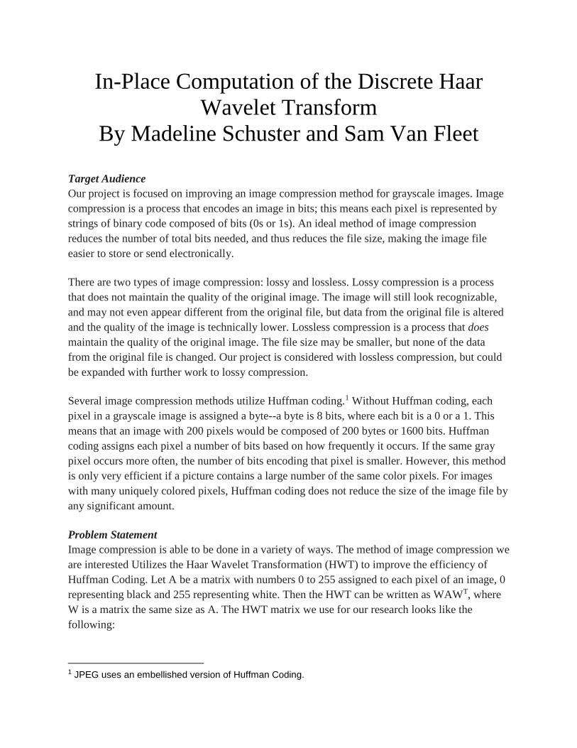
2x2 matrix 4x4 matrix 8x8 matrix

An HWT for one iteration on a generic 4x4 A matrix would look like this:

W A WT

=

Answer

The resulting image from the same WAWT transformation applied on a photo with a much larger

file size would look like this:

Original One iteration of WAWT

The second iteration is done using the upper left block image created in the previous iteration.

Then a WAWT transformation is applied to that image and then replaces the upper left block.

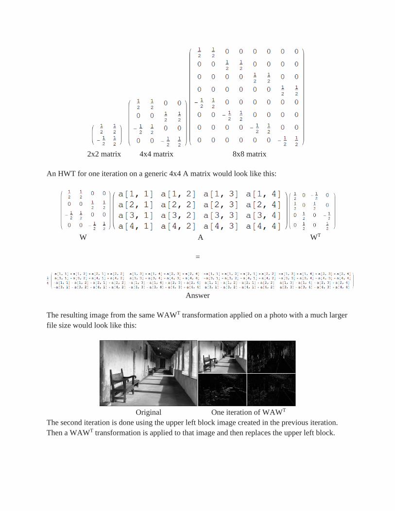
Second Iteration

W A WT

First iteration

W Upper left quadrant of first iteration WT

Upper left quadrant of second iteration

↓

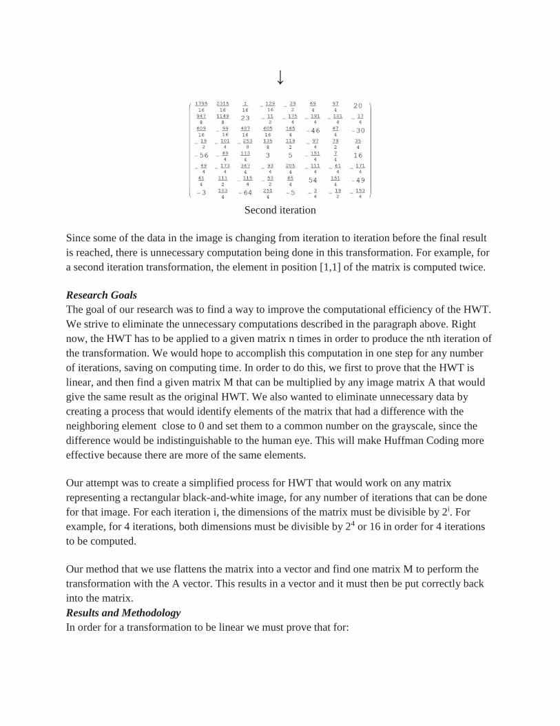
Second iteration

Since some of the data in the image is changing from iteration to iteration before the final result

is reached, there is unnecessary computation being done in this transformation. For example, for

a second iteration transformation, the element in position [1,1] of the matrix is computed twice.

Research Goals

The goal of our research was to find a way to improve the computational efficiency of the HWT.

We strive to eliminate the unnecessary computations described in the paragraph above. Right

now, the HWT has to be applied to a given matrix n times in order to produce the nth iteration of

the transformation. We would hope to accomplish this computation in one step for any number

of iterations, saving on computing time. In order to do this, we first to prove that the HWT is

linear, and then find a given matrix M that can be multiplied by any image matrix A that would

give the same result as the original HWT. We also wanted to eliminate unnecessary data by

creating a process that would identify elements of the matrix that had a difference with the

neighboring element close to 0 and set them to a common number on the grayscale, since the

difference would be indistinguishable to the human eye. This will make Huffman Coding more

effective because there are more of the same elements.

Our attempt was to create a simplified process for HWT that would work on any matrix

representing a rectangular black-and-white image, for any number of iterations that can be done

for that image. For each iteration i, the dimensions of the matrix must be divisible by 2i. For

example, for 4 iterations, both dimensions must be divisible by 24 or 16 in order for 4 iterations

to be computed.

Our method that we use flattens the matrix into a vector and find one matrix M to perform the

transformation with the A vector. This results in a vector and it must then be put correctly back

into the matrix.

Results and Methodology

In order for a transformation to be linear we must prove that for:

i) M(u + v) = M(u) + M(v) for all u, v in the domain of M;

ii) M(cu) = cM(u) for all scalars c and all u in the domain of M.

First condition: M(u + v) = M(u) + M(v)

W(A + B)WT = (W(A + B))WT = (WA + WB)WT = WAWT + WBWT

Second condition:M(cu) = cM(u) for all scalars c and all u in the domain of M

W(cA)WT = (WcA)WT = (cWA)WT = cWAWT

This shows that the transformation is linear. Knowing this information and the following

theorem to be true:

Let T: Rn → Rm be a linear transformation. Then there exists a unique matrix M such that

T(A) = M𝒂 for all 𝒂 in Rn.

Then there exists a unique matrix, M, that completes the transformation WAWT. So now the

transformation can be written as MA for all A, where 𝒂 is a concatenated vector built from A.

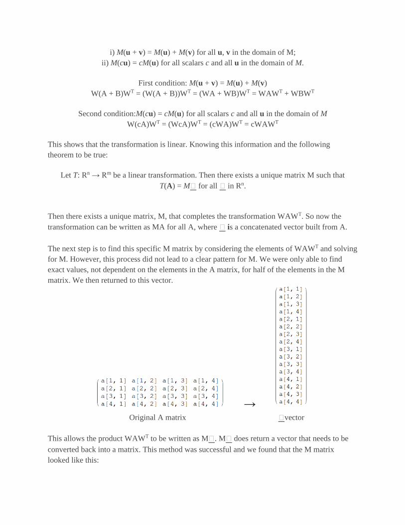
The next step is to find this specific M matrix by considering the elements of WAWT and solving

for M. However, this process did not lead to a clear pattern for M. We were only able to find

exact values, not dependent on the elements in the A matrix, for half of the elements in the M

matrix. We then returned to this vector.

→

Original A matrix 𝒂vector

This allows the product WAWT to be written as M𝒂. M𝒂 does return a vector that needs to be

converted back into a matrix. This method was successful and we found that the M matrix

looked like this:

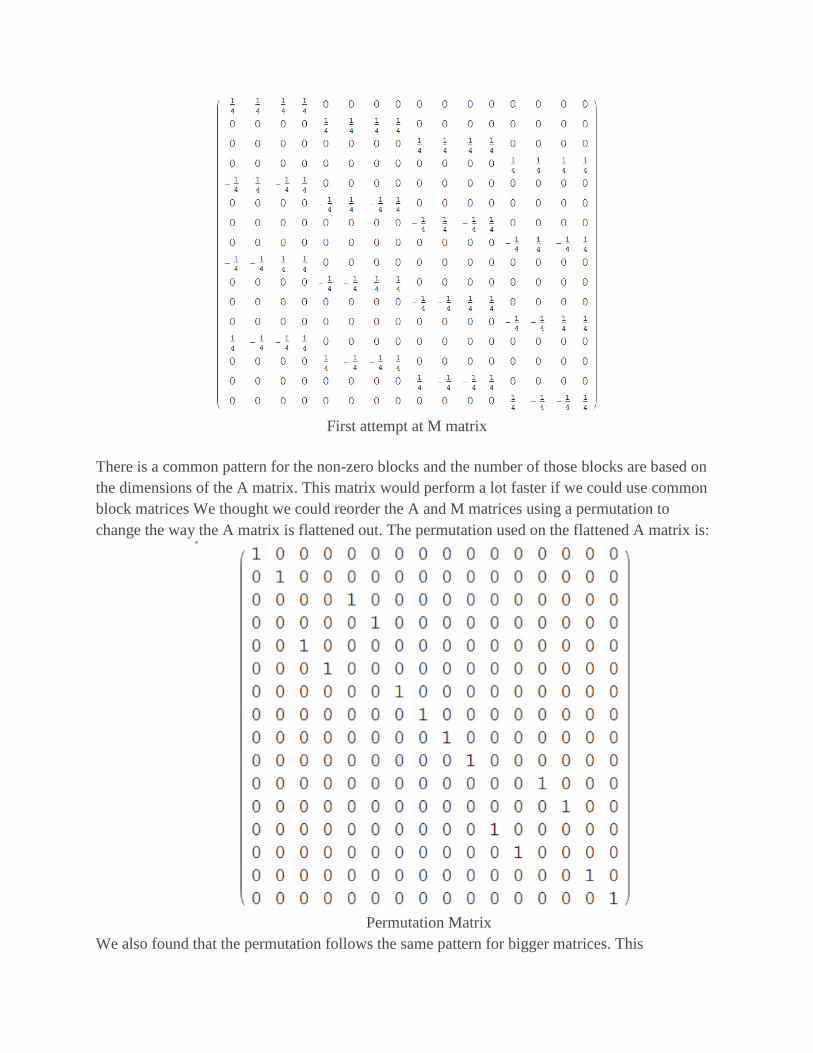
First attempt at M matrix

There is a common pattern for the non-zero blocks and the number of those blocks are based on

the dimensions of the A matrix. This matrix would perform a lot faster if we could use common

block matrices We thought we could reorder the A and M matrices using a permutation to

change the way the A matrix is flattened out. The permutation used on the flattened A matrix is:

Permutation Matrix

We also found that the permutation follows the same pattern for bigger matrices. This

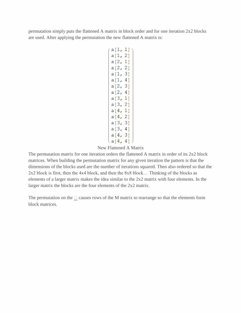
permutation simply puts the flattened A matrix in block order and for one iteration 2x2 blocks

are used. After applying the permutation the new flattened A matrix is:

New Flattened A Matrix

The permutation matrix for one iteration orders the flattened A matrix in order of its 2x2 block

matrices. When building the permutation matrix for any given iteration the pattern is that the

dimensions of the blocks used are the number of iterations squared. Then also ordered so that the

2x2 block is first, then the 4x4 block, and then the 8x8 block… Thinking of the blocks as

elements of a larger matrix makes the idea similar to the 2x2 matrix with four elements. In the

larger matrix the blocks are the four elements of the 2x2 matrix.

The permutation on the 𝒂 causes rows of the M matrix to rearrange so that the elements form

block matrices.

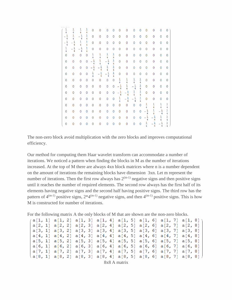
The non-zero block avoid multiplication with the zero blocks and improves computational

efficiency.

Our method for computing them Haar wavelet transform can accommodate a number of

iterations. We noticed a pattern when finding the blocks in M as the number of iterations

increased. At the top of M there are always 4xn block matrices where n is a number dependent

on the amount of iterations the remaining blocks have dimension 3xn. Let m represent the

number of iterations. Then the first row always has 2(m-1) negative signs and then positive signs

until it reaches the number of required elements. The second row always has the first half of its

elements having negative signs and the second half having positive signs. The third row has the

pattern of 4(m-1) positive signs, 2*4(m-1) negative signs, and then 4(m-1) positive signs. This is how

M is constructed for number of iterations.

For the following matrix A the only blocks of M that are shown are the non-zero blocks.

8x8 A matrix

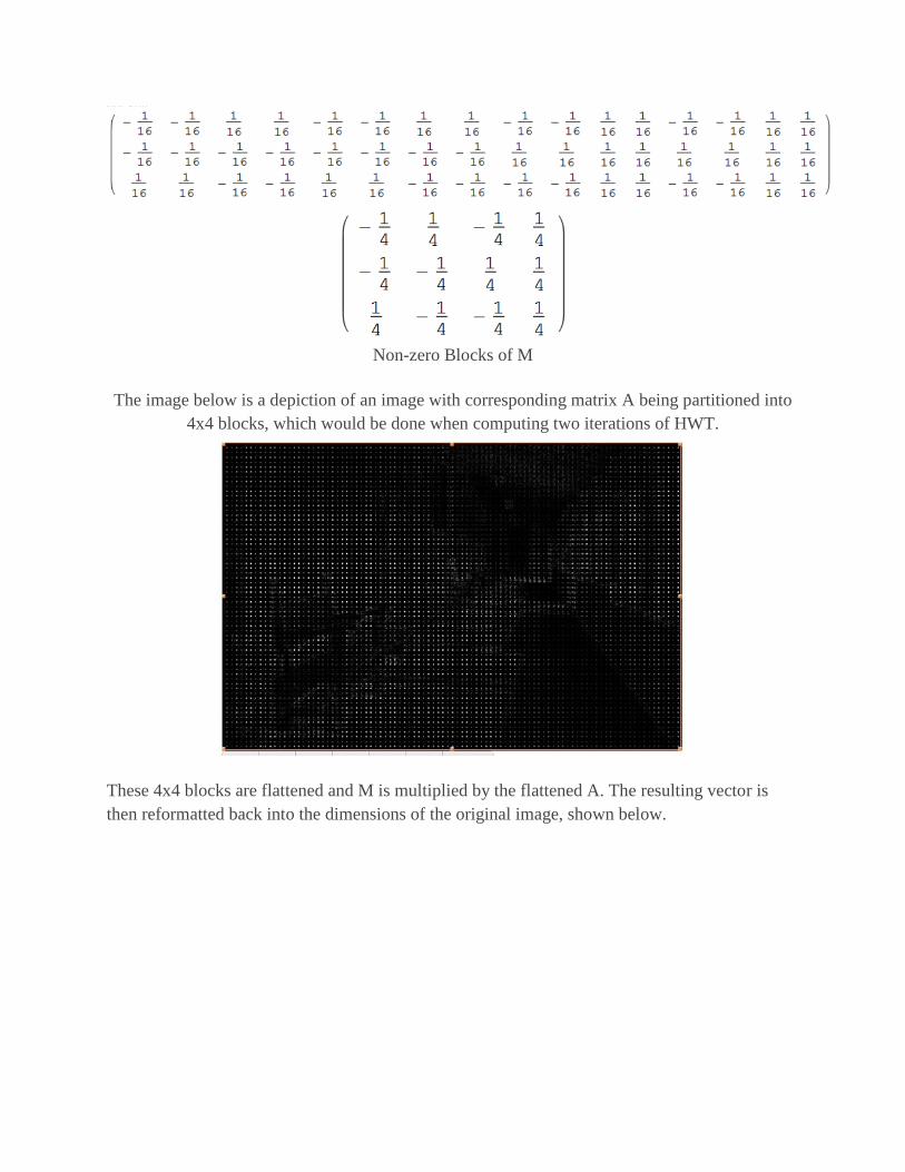
Non-zero Blocks of M

The image below is a depiction of an image with corresponding matrix A being partitioned into

4x4 blocks, which would be done when computing two iterations of HWT.

These 4x4 blocks are flattened and M is multiplied by the flattened A. The resulting vector is

then reformatted back into the dimensions of the original image, shown below.

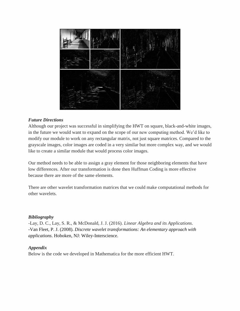
Future Directions

Although our project was successful in simplifying the HWT on square, black-and-white images,

in the future we would want to expand on the scope of our new computing method. We’d like to

modify our module to work on any rectangular matrix, not just square matrices. Compared to the

grayscale images, color images are coded in a very similar but more complex way, and we would

like to create a similar module that would process color images.

Our method needs to be able to assign a gray element for those neighboring elements that have

low differences. After our transformation is done then Huffman Coding is more effective

because there are more of the same elements.

There are other wavelet transformation matrices that we could make computational methods for

other wavelets.

Bibliography

-Lay, D. C., Lay, S. R., & McDonald, J. J. (2016). Linear Algebra and its Applications.

-Van Fleet, P. J. (2008). Discrete wavelet transformations: An elementary approach with

applications. Hoboken, NJ: Wiley-Interscience.

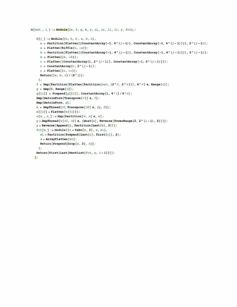
Appendix

Below is the code we developed in Mathematica for the more efficient HWT.