Embed Size (px)
Citation preview

Improving EEG-based Driver Fatigue Classification using Sparse-Deep
Belief Networks
Rifai Chai1*
, Sai Ho Ling1, Phyo Phyo San
2, Ganesh R. Naik
1, Tuan N. Nguyen
1, Yvonne 1
Tran1,3
, Ashley Craig3, Hung T. Nguyen
1 2
1Centre for Health Technologies, Faculty of Engineering and Information Technology, University of 3
Technology, Sydney, NSW 2007, Australia 4
2Data Analytic Department, Institute for Infocomm Research, A*STAR, Singapore 5
3Kolling Institute of Medical Research, Sydney Medical School, The University of Sydney 6
* Correspondence: 7 Dr. Rifai Chai 8
Keywords: electroencephalography, driver fatigue, autoregressive model, deep belief networks, 10
sparse-deep belief networks 11
Abstract 12
This paper presents an improvement of classification performance for electroencephalography 13
(EEG)-based driver fatigue classification between fatigue and alert states with the data collected from 14
43 participants. The system employs autoregressive (AR) modeling as the features extraction 15
algorithm, and sparse-deep belief networks (sparse-DBN) as the classification algorithm. Compared 16
to other classifiers, sparse-DBN is a semi supervised learning method which combines unsupervised 17
learning for modeling features in the pre-training layer and supervised learning for classification in 18
the following layer. The sparsity in sparse-DBN is achieved with a regularization term that penalizes 19
a deviation of the expected activation of hidden units from a fixed low-level prevents the network 20
from overfitting and is able to learn low-level structures as well as high-level structures. For 21
comparison, the artificial neural networks (ANN), Bayesian neural networks (BNN) and original 22
deep belief networks (DBN) classifiers are used. The classification results show that using AR 23
feature extractor and DBN classifiers, the classification performance achieves an improved 24
classification performance with a of sensitivity of 90.8%, a specificity of 90.4%, an accuracy of 25
90.6% and an area under the receiver operating curve (AUROC) of 0.94 compared to ANN 26
(sensitivity at 80.8%, specificity at 77.8%, accuracy at 79.3% with AUC-ROC of 0.83) and BNN 27
classifiers (sensitivity at 84.3%, specificity at 83%, accuracy at 83.6% with AUROC of 0.87). Using 28
the sparse-DBN classifier, the classification performance improved further with sensitivity of 93.9%, 29
a specificity of 92.3% and an accuracy of 93.1% with AUROC of 0.96. Overall, the sparse-DBN 30
classifier improved accuracy by 13.8%, 9.5% and 2.5% over ANN, BNN and DBN classifiers 31
respectively. 32
33
34
35

2
36
1 Introduction 37
Fatigue during driving is a major cause of road accidents in transportation, and therefore poses a 38
significant risk of injury and fatality, not only to the drivers themselves but also to other road users 39
such as passengers, motorbike users, other drivers and pedestrians (Desmond et al., 2012). Driver 40
fatigue reduces the ability to perform essential driving skills such as vehicle steering control, tracking 41
vehicle speed, visual awareness and sufficient selective attention during a monotonous driving 42
condition for a long period of time (Lal and Craig, 2001; Wijesuriya et al., 2007; Craig et al., 2012; 43
Jurecki and Stańczyk, 2014). As a result an automated countermeasure for a driver fatigue system 44
with reliable and improved fatigue classification/detection accuracy is needed to overcome the risk of 45
driver fatigue in transportation (Lal et al., 2003; Vanlaar et al., 2008; Touryan et al., 2013; Touryan et 46
al., 2014; Chai et al., 2016). 47
In the digital age, machine learning can be used to provide automated prediction of driver fatigue. 48
Two approaches can be used in machine learning, which are the regression and classification 49
methods. The goal of regression algorithms is the prediction of continuous values to estimate driving 50
performance (Lin et al., 2005; Touryan et al., 2013; Touryan et al., 2014). The outcome of 51
classification algorithms is to predict the target class, such as the classification between fatigue and 52
non-fatigue/alert states (Lin et al., 2010; Zhang et al., 2014; Chai et al., 2016; Xiong et al., 2016). 53
The aim of this study is to improve the accuracy of the prediction of fatigue and non-fatigue states. 54
As a result, this study focuses on using an advanced classification method for enhancing the accuracy 55
of a fatigue classification system previously studied (Chai et al., 2016). 56
As described in a previous paper (Chai et al., 2016), possible driver fatigue assessment includes 57
psychological and physiological measurements (Lal and Craig, 2001; Borghini et al., 2014). For 58
instance, psychological measurement of driver fatigue involves the need for frequent self-report of 59
fatigue status via brief psychometric questionnaires (Lai et al., 2011). Such an approach would be 60
difficult to implement and may well be biased given its subjective nature (Craig et al., 2006). 61
Physiological measurement of the driver fatigue includes video measurement of the face (Lee and 62
Chung, 2012), brain signal measurement using electroencephalography (EEG) (Lal et al., 2003; Lin 63
et al., 2005; Craig et al., 2012; Chai et al., 2016), eye movement tracking system using camera and 64
electrooculography (EOG) (Hsieh and Tai, 2013) and heart rate measurement using 65
electrocardiography (ECG) (Tran et al., 2009; Jung et al., 2014). 66
Physiological assessment of facial or eye changes using video recording of the driver’s face may lead 67
to privacy issues. Physiological measurement strategies like monitoring eye blink rates using EOG 68
and heart rate variability (HRV) using ECG have been shown to reliably detect fatigue (Tran et al., 69
2009; Hsieh and Tai, 2013). EEG has also been shown to be a reliable method of detecting fatigue, 70
as it directly measures neurophysiological signals that are correlated with mental fatigue (Wijesuriya 71
et al., 2007; Craig et al., 2012; Zhang et al., 2014; Chuang et al., 2015; He et al., 2015; Xiong et al., 72
2016). Recently, we have shown a classification of EEG-based driver fatigue with the inclusion of 73
new ICA based pre-processing with a promising classification result (Chai et al., 2016), however, it 74
was concluded the classification accuracy needs to be improved. As a result, this paper will extend 75
the work on a potential EEG-based countermeasure driver fatigue system with an improved 76
classification of fatigue vs. alert states. 77

3
An EEG-based classification countermeasure system requires several components including EEG 78
signal measurement, signal pre-processing, feature extraction, and classification modules. For feature 79
extraction in EEG analysis, frequency domain data has been widely explored (Lal and Craig, 2001; 80
Craig et al., 2012). Power spectral density (PSD) methods are popular for converting the time domain 81
of EEG signal into the frequency domain (Demandt et al., 2012; Lin et al., 2014). Alternatively, an 82
autoregressive (AR) modelling parametric approach can also be used for feature extraction in an EEG 83
classification system (McFarland and Wolpaw, 2008; Chai et al., 2016; Wang et al., 2016). The 84
advantage of AR modelling is its inherent capacity to model the peak spectra that are characteristic of 85
the EEG signals and it is an all-pole model making it efficient for resolving sharp changes in the 86
spectra. In our previous finding, an AR modelling feature extractor provided superior classification 87
results compared to PSD for EEG-based driver fatigue classification (Chai et al., 2016). Therefore, in 88
this paper, we present the results of applying AR for modeling feature extraction in order to improve 89
the accuracy the classification algorithm. The PSD method is also included for comparison. For the 90
classification, non-linear methods, such as artificial neural networks (ANN), have been used widely 91
in a variety of applications involving EEG (Nguyen, 2008; Casson, 2014). Bayesian neural networks 92
(BNN) have also been used in EEG-based driver fatigue classification (Chai et al., 2016). The 93
Bayesian regularization framework is able to enhance the generalization of neural networks training 94
regardless of finite and/or noisy data. 95
Recent attention has been focused on improvement of an ANN approach called deep belief networks 96
(DBN) (Hinton et al., 2006; Hinton and Salakhutdinov, 2006; Bengio, 2009; LeCun et al., 2015), 97
which involves a fast, unsupervised learning algorithm for the deep generative model and supervised 98
learning for a discriminative model. The key advantage of this algorithm is the layer-by-layer training 99
for learning a deep hierarchical probabilistic model efficiently as well as a discriminative fine tuning 100
algorithm to optimize performance on the classification problems (Bengio, 2009; LeCun et al., 2015). 101
A DBN classifier is a promising strategy for improving classification of problems including hand-102
writing character classification (Hinton et al., 2006), speech recognition (Mohamed et al., 2010; 103
Hinton et al., 2012), visual object recognition (Krizhevsky et al., 2012) and other biomedical 104
applications (O'Connor et al., 2013; Stromatias et al., 2015). The training of the DBN is based on the 105
restricted Boltzmann machine (RBM) with layers-wise training of the network per layer at a time 106
from the bottom up (Hinton et al., 2006). Furthermore, the original RBM approach tended to learn a 107
distributed non-sparse representation. A modified version of the RBM using sparse-RBM to form a 108
sparse-deep belief network (sparse-DBN) has shown promising results for modelling low-order 109
features as well as higher-order features for the application of image classification with improved 110
accuracy (Lee et al., 2008; Ji et al., 2014). As a result of this promising advance in classification of 111
complex features, this paper further investigates the classification of EEG signals associated with 112
driver fatigue using the sparse-DBN. For comparison purposes, the results from several different 113
classifiers are included to determine which algorithms are superior with the highest classification 114
performance. 115
The main contribution of this paper is the combination of the AR modelling feature extractor and 116
sparse-DBN classifier which have not been explored previously for EEG-based driver fatigue 117
classification, with the objective of enhancing the classification performance over past attempts (Chai 118
et al., 2016). The motivation to utilize the sparse-DBN classifier was to investigate its potential 119
superiority for classifying fatigue, in comparison to other classifiers. Sparse-DBN is a semi 120
supervised learning method that combines unsupervised learning for modelling the feature in the pre-121
training layer and supervised learning for discriminating the feature in the following layer. 122
Incorporating the sparsity in sparse-DBN, achieved with a regularization term that penalizes a 123
deviation of the expected activation of hidden units from a fixed low-level, prevents the network 124

4
from overfitting and is able to learn low-level structures as well as high-level structures (Ji et al., 125
2014). The structure of this paper is as follows: section II covers the background and methodology 126
including general structure, EEG experiment and pre-processing, feature extraction and classification. 127
Section III describes results, followed by section IV for discussion and section V for the conclusions. 128
2 Background and Methodology 129
2.1 General Structure 130
The general structure for the EEG-based driver fatigue classification used in this paper is shown in 131
FIGURE 1 which is divided into four components: (i) the first component involves EEG data 132
collection in a simulated driver fatigue environment; (ii) the second component involves data pre-133
processing for removing EEG artifact and the moving window segmentation; (iii) the third 134
component involves the features extraction module that converts the signals into useful features; (iv) 135
the fourth component involves the classification module to process the feature and which translates 136
into output via training and classification procedures. The output of the classification comprises two 137
states: fatigue state and alert (non-fatigue) state. 138
FIGURE 1 | General structure EEG-based driver fatigue classification in this study 139
2.2 EEG Data Collection 140
The EEG data collection has been described in a previous paper (Chai et al., 2016). The study was 141
approved by the Human Research Ethics Committee of the University of Technology Sydney (UTS) 142
obtained from previous experiments of driver fatigue study (Craig et al., 2006; Wijesuriya et al., 143
2007; Craig et al., 2012). The dataset contains electrophysiological data from 43 healthy participants 144
aged between 18 and 55 years who had a current driver’s licence. The study involved continuous 145
measurement taken during a monotonous simulated driving task followed by post EEG measures and 146
post-subjective self-report of fatigue. For the simulated driving task, the divided attention steering 147
simulator (DASS) from Stowood scientific instruments was used (Craig et al., 2012). Participants 148
were asked to keep driving at the centre of the road in the simulation task. The participants were also 149
required to respond to a target number that appeared in any of the four corners of the computer screen 150
in front of the participants when they were driving in the experiment, so as to record reaction time. 151
FIGURE 2 | Moving window segmentation for driver fatigue study 152
The simulation driving task was terminated if the participant drove off the simulated road for greater 153
than 15 seconds, or if they showed consistent facial signs of fatigue such as head nodding and 154
extended eyes closure, both determined by analysis of participants’ faces that occurred throughout 155
the experiment. Three methods were used to validate fatigue occurrence: (i) using video monitoring 156
for consistent physiological signs of fatigue such as tired eyes, head nodding and extended eye 157
closure, verified further by EOG analysis of blink rate and eye closure; (ii) using performance 158
decrements such as deviation off the road, and (iii) using validated psychometrics such as the Chalder 159
Fatigue Scale and the Stanford Sleepiness Scale. Two participants who did not meet the criterion of 160
becoming fatigued were excluded from the dataset. The validation of fatigue versus non-fatigue in 161
these participants has been reported in prior studies (Craig et al., 2006; Craig et al., 2012). The EEG 162
signals were recorded using a 32-channel EEG system, the Active-Two system (Biosemi) with 163
electrode positions at: FP1, AF3, F7, F3, FC1, FC5, T7, C3, CP1, CP5, P7, P3, PZ, PO3, O1, OZ, 164
O2, PO4, P4, P8, CP6, CP2, C4, T8, FC6, FC2, F4, F8, AF4, FP2, FZ and CZ. The recorded EEG 165
data was down sampled from 2048Hz to 256Hz. 166

5
2.3 Data Pre-processing and Segmentation 167
For the alert status, the first 5 mins of EEG data was selected when the driving simulation task began. 168
For the fatigue status, the data was selected from the last 5 mins of EEG data before the task was 169
terminated, after consistent signs of fatigue were identified and verified. Then in each group of data 170
(alert and fatigue), 20s segments were taken with the segment that was chosen being the first 20 171
seconds where EEG signals were preserved. For the sample this was all within the first 1 minute of 172
the 5 minutes selected. Further artifact removal using an ICA-based method was used to remove 173
blinks, heart and muscle artifact. As a result, 20s of the alert state and 20s of the fatigue state data 174
were available from each participant. 175
In the pre-processing module before feature extraction, the second-order blind identification (SOBI) 176
and canonical correlation analysis (CCA) were utilized to remove artifacts of the eyes, muscle and 177
heart signals. The pre-processed data were segmented by applying a moving window of 2s with 178
overlapping 1.75s to the 20s EEG data which provided 73 overlapping segments for each state 179
(fatigue and alert states) as shown in FIGURE 2. The pre-processing segments were used in the 180
feature extraction module as described in next section. 181
2.4 Feature Extraction 182
For comparison purposes and validity of previous work, a feature extractor using the power spectral 183
density (PSD), a widely used spectral analysis of feature extractor in fatigue studies, is provided in 184
this paper. 185
An autoregressive (AR) model was also applied as a features extraction algorithm in this study. AR 186
modelling has been used in EEG studies as an alternative to Fourier-based methods, and has been 187
reported to have improved classification accuracy in previous studies compared to spectral analysis 188
of the feature extractor (Brunner et al., 2011; Chai et al., 2016). The advantage of AR modelling is its 189
inherent capacity to model the peak spectra that are characteristic of the EEG signals and it is an all-190
pole model making it efficient for resolving sharp changes in the spectra. The fast Fourier transform 191
(FFT) is a widely used nonparametric approach that can provide accurate and efficient results, but it 192
does not have acceptable spectral resolution for short data segments (Anderson et al., 2009). AR 193
modelling requires the selection of the model order number. The best AR order number requires 194
consideration of both the signal complexity and the sampling rate. If the AR model order is too low, 195
the whole signal cannot be captured in the model. On the other hand, if the model order is too high, 196
then more noise is captured. In a previous study, the AR order number of five provided the best 197
classification accuracy (Chai et al., 2016). The calculation of the AR modelling was as follows: 198
�̂�(𝒕) = ∑ 𝒂(𝒌)�̂�(𝒕 − 𝒌) + 𝒆(𝒕)
𝑷
𝒌=𝟏
(𝟏)
where �̂�(𝒕) denotes EEG data at time (t), P denotes the AR order number, e(t) denotes the white 199
noise with zero means error and finite variance, and a(k) denotes the AR coefficients. 200
2.5 Classification Algorithm 201
The key feature of DBN is the greedy layer-by-layer training to learn a deep, hierarchical model 202
(Hinton et al., 2006). The main structure of the DBN learning is the restricted Boltzmann machine 203
(RBM). A RBM is a type of Markov random field (MRF) which is a graphical model that has a two-204

6
layer architecture in which the observed data variables as visible neurons are connected to hidden 205
neurons. A RBM is as shown in which m visible neuron (v=(v1, v2, v3,…,vm)) and n hidden neurons 206
(h=(h1, h2,…, hn)) are fully connected via symmetric undirected weights and there is no intra-layer 207
connections within either the visible or the hidden layer. 208
The connections weights and the biases define a probability over the joint states of visible and hidden 209
neurons through energy function E(v,h), defined as follows: 210
𝑬(𝒗, 𝒉; 𝜽) = − ∑
𝒎
𝒊=𝟏
∑ 𝒘𝒊𝒋𝒗𝒊
𝒏
𝒋=𝟏
𝒉𝒋 − ∑ 𝒂𝒊𝒗𝒊
𝒎
𝒊=𝟏
− ∑ 𝒃𝒋𝒉𝒊
𝒏
𝒋=𝟏
(𝟐)
where wij denotes the weight between vi and hj for all i {1,…, m} and j {1,…, n}; ai and bj are 211
the bias term associated with the ith
and jth
visible and hidden neurons; {W,b,a} is the model 212
parameter with symmetric weight parameters Wnm. 213
For RBM training, the gradient of log probability of a visible vector (v) over the weight wij with the 214
updated rule calculated by constructive divergence (CD) method is as follows: 215
∆𝒘𝒊𝒋 = (⟨𝒗𝒊𝒉𝒋⟩𝒅𝒂𝒕𝒂 − ⟨𝒗𝒊𝒉𝒋⟩𝒓𝒆𝒄𝒐𝒏) (𝟑)
where is a learning rate, ⟨𝒗𝒊𝒉𝒋⟩𝒓𝒆𝒄𝒐𝒏 is the reconstruction of original visible units which is calculated 216
by setting the visible unit to a random training vector. The updating of the hidden and visible states is 217
considered as follows: 218
𝒑(𝒉𝒋 = 𝟏 | 𝒗) = 𝝈 (𝒃𝒋 + ∑ 𝒗𝒊𝒘𝒊𝒋
𝒊
) (𝟒)
𝒑(𝒗𝒊 = 𝟏 | 𝒉) = 𝝈 (𝒂𝒊 + ∑ 𝒉𝒋𝒘𝒊𝒋
𝒊
) (𝟓)
where is the logistic sigmoid function. 219
The original RBM tended to learn a distributed, non-sparse representation of the data, however 220
sparse-RBM is able to play an important role in learning algorithms. In an information-theoretic 221
sense, sparse representations are more efficient than the non-sparse ones, allowing for varying of the 222
effective number of bits per example and able to learn useful low-level and high-level feature 223
representations for unlabeled data (ie. unsupervised learning) (Lee et al., 2008; Ji et al., 2014). 224
This paper uses the sparse-RBM to form the sparse-DBN for EEG-based driver fatigue classification. 225
The sparsity in sparse-DBN is achieved with a regularization term that penalizes a deviation of the 226
expected activation of hidden units from a fixed low-level, which prevents the network from 227
overfitting, as well as allowing it to learn low-level structures as well as high-level structures (Ji et 228
al., 2014). The sparse-RBM is obtained by adding a regularization term to the full data negative log 229
likelihood with the following optimization: 230
𝐦𝐢𝐧{𝒘𝒊𝒋𝒂𝒊𝒃𝒋}
𝑬(𝒗, 𝒉, 𝜽) − ∑ 𝐥𝐨 𝐠 ∑ 𝑷(𝒗(𝒍), 𝒉(𝒍))
𝒉
𝒎
𝒍=𝟏
+ 𝝀 ∑ |𝒑 −𝟏
𝒎∑ 𝔼 [𝒉𝒋
(𝒍)|𝒗(𝒍)]
𝒎
𝒍=𝟏
|
𝟐𝒏
𝒋=𝟏
(𝟔)

7
where 𝔼[.] is the conditional expectation given the data, λ is a regularization constant and p is a 231
constant controlling the sparseness of the hidden neurons hj. The DBN is constructed by stacking a 232
predefined number of RBMs to allow each RBM model in the sequence to receive a different 233
representation of the EEG data. The modelling between visible input (v) and N hidden layer hk is as 234
follows: 235
𝑷(𝒗, 𝒉𝟏, … , 𝒉𝒍) = (∏ 𝑷([𝒉(𝒌)|𝒉(𝒌+𝟏)])
𝒍−𝟐
𝒌=𝟎
) 𝑷(𝒉𝒍−𝟏, 𝒉𝒍) (𝟕)
where v = h0, P(h
k|h
k+1) is a conditional distribution for the visible units conditioned on the hidden 236
units of the RBM at level k and P(hl-1
,hl) is the visible-hidden joint distribution at the top-level RBM. 237
Two training types of the RBM can be used: generative and discriminative. The generative training 238
of RBM is used as pre-training with un-supervised learning rule. After greedy layer-wise 239
unsupervised learning, the DBN can be used for discriminative ability using the supervised learning. 240
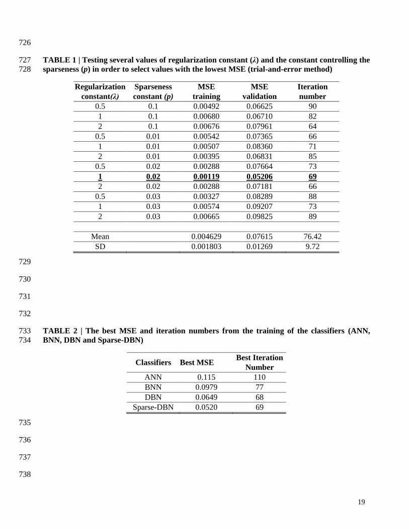
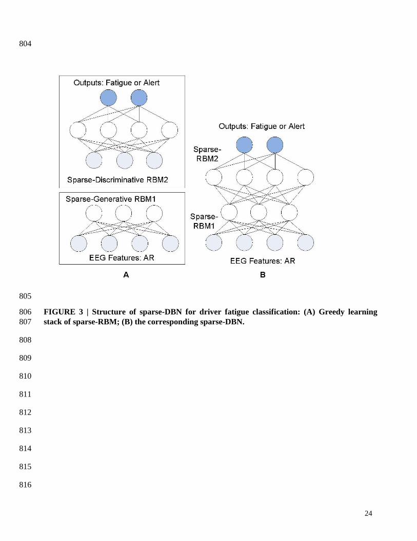
This paper uses a sparse variant of DBN with 2 layers of semi supervised sparse-DBN as shown in 241
FIGURE 3 with the first layer using the sparse-RBM for generative mode (un-supervised learning) 242
and the second layer using the sparse-RBM in discriminative mode (supervised learning). After 243
layer-by-layer training in DBN, an ANN with back-propagation method is used through the whole 244
classifier to fine-tune the weights for optimal classification. 245
FIGURE 3 | Structure of sparse-DBN for driver fatigue classification: (A) Greedy learning 246
stack of sparse-RBM; (B) the corresponding sparse-DBN. 247
The performance indicators, including, sensitivity or true positive rate (TPR= TP/(TP+FN)), 248
specificity or true negative rate (TNR=TN/(TN+FP)) and accuracy (TP+TN)/(TP+TN+FP+FN), were 249
used for the performance measurement. TP (true positive) denotes the number of the fatigue data 250
correctly classified as fatigue state. FP (false positive) is the number of alert datasets classified as a 251
fatigue state. TN (true negative) is number of alert datasets correctly classified as an alert state. FN 252
(false negative) is the fatigue datasets classified as an alert state. 253
For network learning generalization, we presented the results based on two cross-validation 254
techniques: an early stopping technique and k-fold cross-validation. The early stopping technique 255
used the ‘hold-out cross validation’ – one of the widely used cross validations techniques. Basically, 256
it divided the dataset into three subsets (training, validation and testing sets). The model is trained 257
using the training set while the validation set is periodically used to evaluate the model performance 258
to avoid over-fitting/over-training. The accuracy of the testing set is used as the result of the model’s 259
performance. Another cross validation technique is known as k-fold cross-validation (k=3). In k-fold 260
cross-validation (k=3), the dataset is divided into three equal (or near equal) sized folds. The training 261
of the network uses 2 folds and the testing the network uses the remaining fold. The process of 262
training and testing is repeated for three possible choices of the subset omitted from the training. The 263
average performance on the three omitted subsets is then used as an estimate of the generalization 264
performance. 265
Furthermore, a receiver operating characteristic (ROC) graph is used to evaluate further the 266
performance of the proposed method with the compared method for this study. The areas under the 267
curve of the ROC (AUROC) were also computed to evaluate quantitatively the classification 268
performance. 269

8
270
3 Results 271
From the 32-EEG channel dataset for the 43 participants (2 participants who did not meet the 272
criterion of becoming fatigued were excluded from original 45 participants), 20s of alert state and 20s 273
of fatigue state data were available from each participant. This was fed to the pre-processing module 274
including artifact removal and a 2s moving window segmentation with overlapping 1.75s to the 20s 275
EEG data, providing 73 overlapping segments for each state. As a result, from the 43 participants, a 276
total 6278 units of datasets were formed for the alert and fatigue states (each state having 3139 units). 277
The segmented datasets were fed to the feature extraction module. AR modelling with the order 278
number of 5 was used for the feature extractor as it provided an optimum result from the previous 279
study (Chai et al., 2016). The size of the AR features equaled the AR order number multiplied with 280
32 units of EEG channels, thus the AR order number of 5 resulted in 160 units of the AR features. 281
For comparison and validity purposes, this paper includes the PSD, a popular feature extractor in the 282
EEG classification for driver fatigue classification. The spectrum of EEG bands consisted of: delta 283
(0.5-3Hz), theta (3.5-7.5Hz), alpha (8-13Hz) and beta activity (13.5-30Hz). The total power for each 284
EEG activity band was used for the features that were calculated using the numerical integration 285
trapezoidal method, providing 4 units of power values. This resulted in 128 units of total power of 286
PSD for the 32 EEG channels used. 287
The variant of standard DBN algorithm, sparse-DBN with semi supervised learning used in this 288
paper, comprised of one layer of sparse-RBM with the generative type learning and the second layer 289
of sparse-RBM with discriminative type of learning. The training of the sparse-DBN is done layer-290
by-layer. The ANN with back-propagation method was used to fine-tune the weights for optimal 291
classification. 292
TABLE 1 | Testing several values of regularization constant (λ) and the constant controlling the 293
sparseness (p) in order to select values with the lowest MSE (trial-and-error method) 294
For the discriminative learning of sparse-DBN, the total 6278 datasets were divided into three 295
subsets with similar amounts of number sets: training (2093 sets) validation (2093 sets) and testing 296
sets (2092 sets). The generative learning of sparse-DBN uses unlabeled data from the training sets. 297
For the training of the sparse-DBN using the learning rate () of 0.01, the maximum epoch is set to 298
200, with a regularization constant (λ) of 1, and the constant controlling the sparseness (p) of 0.02. 299
The selection of these training parameters was chosen by trial-and-error, with the chosen values 300
achieving the best training result. TABLE 1 shows the selection of the regularization constant (λ), 301
with the chosen value of 1 and the constant controlling the sparseness (p) with the chosen value of 302
0.02, providing lowest the mean square error (MSE) values of 0.00119 (training set) and 0.0521 303
(validation set) with the iteration number of 69. The average of the MSE values was 0.0046±0.0018 304
(training set), and 0.0760±0.0124. 305
FIGURE 4 |Plot of the training and validation MSE for early stopping of classifiers: (A) MSE 306
training and validation of ANN. (B) MSE training of BNN. (C) MSE training of DBN in hidden 307
layer 1 (Generative mode). (D) MSE training of sparse-DBN in hidden layer 1 (Generative 308
mode). (E) MSE training and validation of DBN in hidden layer 2 (Discriminative mode). (F) 309
MSE training and validation of DBN in hidden layer 2 (Discriminative mode). 310

9
TABLE 2 | The best MSE and iteration numbers from the training of the classifiers (ANN, 311
BNN, DBN and Sparse-DBN) 312
In order to prevent overfitting/over-training in the network, a validation-based early stopping method 313
was used for the proposed classifier of sparse-DBN. The plot of the mean square error (MSE) 314
training set and validation set are shown in FIGURE 4 for classification using AR and sparse-DBN. 315
TABLE 2 shows the best performance of the training in term of the MSE values and iteration 316
numbers. For comparison, the results for ANN, BNN and DBN classifier are also included. 317
ANN, DBN and sparse-DBN classifiers utilized the early stopping framework (with the dataset 318
divided into training validation and test sets) to prevent the overfitting problem, except for BNN 319
(where the dataset was divided into training and testing). The BNN used a different framework for 320
preventing the overfitting problem utilizing adaptive hyper-parameters in the cost function to prevent 321
the neural network weight from being too large, which would have resulted in poor generalization. 322
As a result, the validation set is not required for the BNN. A detailed analysis of BNN for EEG based 323
driver fatigue classification has been addressed in our previous study (Chai et al., 2016). The core 324
parameters for the training classifiers (ANN, BNN, DBN and sparse-DBN) are the ANN-based 325
classifier which includes the number of hidden nodes, an activation function and learning rate. In the 326
BNN classifier, an additional hyper-parameter is introduced to fine tune the optimal structure of the 327
ANN. Further, in the sparse-DBN classifier, the regulation constant and constant controlling of 328
sparseness were introduced for the training the DBN classifier. The DBN and sparse-DBN used two 329
hidden layers: the first hidden layer as generative mode (un-supervised learning) and second hidden 330
layer as discriminative mode (supervised learning). 331
The mean square error (MSE) of the training set decreased smoothly. Using ANN classifier, the 332
training network stopped after 100 iterations as the MSE validation set reached a maximum fail of 10 333
times the increment value to ensure no over-training happened with the best validation MSE at 0.115. 334
Using a BNN classifier, the training network stopped after 77 iterations as the conditions are met 335
with the BNN parameters with the best validation MSE at 0.0979. Using a DBN classifier in the first 336
hidden layer (generative mode), the training network stopped after 200 iterations with best MSE at 337
0.434. Using a DBN classifier in the second hidden layer (discriminative mode), the training 338
network stopped after 68 iterations as the MSE validation set reached maximum fail of 10 times 339
increment value to ensure no over-training happened with the best validation MSE at 0.0649. Using 340
the proposed method of sparse-DBN classifier in the first hidden layer (generative mode), the training 341
network stopped after 200 iterations with the best of MSE at 0.388. Using the proposed method of 342
sparse-DBN classifier in the second hidden layer (discriminative mode), the training network stopped 343
after 69 iterations as the MSE validation set reached maximum fail of 10 times increment value to 344
ensure no over-training happened, with the best validation MSE at 0.0520. 345
Using the classification results from the validation set, the optimal number of hidden neurons of the 346
sparse-DBN is shown in FIGURE 5. For the PSD feature extraction, using 10 hidden nodes resulted 347
in the best classification performance. For the AR feature extraction, using 15 hidden nodes produced 348
the best classification performance. These optimal hidden nodes were then used for the training of the 349
network to classify the test set. Also, the results using a different number of layers (two layers, three 350
layers, five layers and ten layers) are also provided in FIGURE 5, with the 2 layers (generative mode 351
for the first layer and discriminative mode for second layer) providing the optimal number of layers 352
in this study. This figure shows that using a higher number of layers (three layers, five layers and ten 353
layers) results in a lower accuracy compared to results of using only two layers. Therefore, the two 354
layers sparse-DBN was the chosen architecture providing the higher accuracy. The optimal size of 355

10
sparse-DBN to classify the PSD features of the EEG-based driver fatigue is [128-10-10-2] and the 356
optimal size of sparse DBN to classify the AR feature is [160-15-15-2]. TABLE 3 shows the results 357
for the classification of the fatigue state vs. alert state using AR feature extractor and sparse-DBN 358
classifier. For a feature extractor comparison and validity of previous result, the result of the 359
classification using PSD feature extractor method is included. Also for classifier comparison, the 360
classification results using original DBN, BNN and ANN are given. 361
FIGURE 5 | Plot of the optimal number hidden nodes and layers 362
First, for the artificial neural network (ANN) classifier: (i) ANN with PSD, for the fatigue data, of a 363
total with 1046 units of actual fatigue dataset, 782 units were correctly classified as fatigue states 364
(true positive: TP), resulting in a sensitivity of 74.8%. For the alert group, of a total of 1046 units of 365
actual alert dataset, 731 units of alert data were correctly classified as alert state (true negative: TN), 366
resulting in a specificity of 69.9%. The combination of ANN and PSD resulted in an accuracy of 367
72.3%. (ii) ANN with AR, for the fatigue group, of a total of 1046 units of actual fatigue dataset, 845 368
units of fatigue data were correctly classified as fatigue states (TP), resulting in a sensitivity of 369
80.8%. For the alert group, of a total of 1046 units of actual alert dataset, 814 units of alert data were 370
correctly classified as alert states (TN), resulting in a specificity of 77.8%, while the combination of 371
ANN with AR resulted in an improved accuracy of 79.3% compared to ANN with PSD. 372
Second, for the Bayesian neural networks (BNN) classifier: (i) BNN with PSD achieved an 373
improvement compared to ANN with PSD, and for the fatigue group, of a total of 1046 units of 374
actual fatigue dataset, 808 units of fatigue data were correctly classified as fatigue states (TP), 375
resulting in a sensitivity of 77.2%. For the alert state, of a total of 1046 units of actual alert dataset, 376
791 units of alert data were correctly classified as alert state (TN), resulting in a specificity of 75.6%. 377
The combination BNN with PSD resulted in an accuracy of 76.4%. (ii) BNN with AR achieved an 378
improvement compared to ANN with AR, and ANN with PSD. BNN with PSD, for the fatigue state, 379
of a total of 1046 units of actual fatigue data, 882 units were correctly classified as fatigue states 380
(TP), resulting in a sensitivity of 84.3%. For the alert state, of a total of 1046 units of actual alert 381
data, 868 units of alert data were correctly classified as alert states (TN), resulting in a specificity of 382
83%. The combination BNN with AR resulted in an accuracy of 83.6%. 383
TABLE 3 | Results classification fatigue state versus alert state for the test set on different 384
feature extractors and classifiers 385
Third, when using the deep belief network (DBN) classifier: (i) DBN with PSD achieved a further 386
improvement compared to BNN with PSD, ANN with PSD and ANN with AR; for the fatigue state, 387
of a total of 1046 units of actual fatigue data, 873 units of fatigue data were correctly classified as 388
fatigue states (TP), resulting in a sensitivity of 83.5%. For the alert state, of a total of 1046 units of 389
actual alert data, 833 units of alert data were correctly classified as alert state (TN), resulting in a 390
specificity of 79.6%. The combination DBN with PSD resulted in an accuracy of 81.5%. (ii) DBN 391
with AR achieved further improvement compared to BNN with AR, ANN with AR, DBN with PSD, 392
BNN with PSD and ANN with PSD, for the fatigue state, of a total of 1046 units of actual fatigue 393
data, 950 units of fatigue data were correctly classified as fatigue states (TP), resulting in a sensitivity 394
of 90.8%. For the alert state, of a total of 1046 units of actual alert data, 946 units of alert data were 395
correctly classified as alert states (TN), resulting in a specificity of 90.4%. The combination of DBN 396
with AR resulted in an accuracy of 90.6%. 397

11
Fourth, using sparse deep belief networks (sparse-DBN): (i) sparse-DBN with PSD achieved 398
additional improvements compared to DBN with PSD, BNN with PSD, ANN with PSD, BNN with 399
AR and ANN with AR; for the fatigue state, of a total of 1046 units of actual fatigue data, 919 units 400
of fatigue data were correctly classified as fatigue states (TP), resulting in a sensitivity of 87.9%. For 401
the alert state, of a total of 1046 units of actual alert dataset, 855 units of alert data were correctly 402
classified as alert state (TN), resulting in a specificity of 81.7%. The combination sparse-DBN with 403
PSD resulted in an accuracy of 84.8%. (ii) sparse-DBN with AR achieved the most superior result to 404
the other classifier and feature extractor combination with the fatigue state, of a total of 1046 units 405
of actual fatigue data, 982 units of fatigue data were correctly classified as fatigue states (TP), 406
resulting in a sensitivity of 93.9%. For the alert state, of a total of 1046 units of actual alert data, 965 407
units of alert data were correctly classified as alert states (TN), resulting in a specificity of 92.3%. 408
The combination sparse-DBN with AR resulted in best accuracy of 93.1% compared to the other 409
classifier and feature extractor combinations. 410
4 Discussion 411
In summary, using the PSD feature extractor: (i) compared to the ANN classifier, the sparse-DBN 412
classifier improved the classification performance with sensitivity by 13.1% (from 74.8% to 87.9%), 413
specificity by 11.8% (from 69.9% to 81.7%) and accuracy by 12.5% (from 72.3% to 84.8%); (ii) 414
compared to the BNN classifier, the sparse-DBN resulted in improved performance indicators for 415
sensitivity by 10.7% (from 77.2% to 87.9%), specificity by 6.1% (from 75.6% to 81.7%) and 416
accuracy by 8.4% (from 76.4% to 84.8%); (iii) compared to the DBN classifier, the sparse-DBN 417
resulted in improved performance indicators for sensitivity by 4.4% (from 83.5% to 87.9%), 418
specificity by 2.1% (from 79.6% to 81.7%) and accuracy by 3.3% (from 81.5% to 84.8%). 419
Further, using the AR feature extractor: (i) compared to the ANN classifier, the sparse-DBN 420
classifier improved the classification performance with sensitivity by 13.1% (from 80.8% to 93.9%), 421
specificity by 14.5% (from 77.8% to 92.3%) and accuracy by 13.8% (from 79.3% to 93.1%); (ii) 422
compared to the BNN classifier, the sparse-DBN resulted in improved performance indicators for 423
sensitivity by 9.6% (from 84.3% to 93.9%), specificity by 9.3% (from 83.0% to 92.3%) and accuracy 424
by 9.5% (from 83.6% to 93.1%); (iii) compared to the DBN classifier, the sparse-DBN resulted in 425
improved performance indicators for sensitivity by 3.1% (from 90.8% to 93.9%), specificity by 1.9% 426
(from 90.4% to 92.3%) and accuracy by 2.5% (from 90.6% to 93.1%). 427
The result of sensitivity (TPR) and specificity (TNR) analyses can also be viewed as the false 428
positive rate (FPR=1−specificity) and false negative rate (FNR = 1−sensitivity). The FPR is the rate 429
of the non-fatigue (alert) state being incorrectly classified as fatigue state. The FNR is the rate of 430
fatigue state being incorrectly classified as an alert state. As a result, the proposed classifier (sparse-431
DBN) with the AR feature extractor resulted in a sensitivity (TPR) of 93.9%, FNR of 6.1%, 432
specificity (TNR) of 92.3% and FPR of 7.7%. For a real-time implementation, an additional 433
debounce algorithm could be implemented. By adding a debounce component, it masks multiple 434
consecutive false positive detection that may decrease the FPR (Bashashati et al., 2006). The real-435
time implementation with a debounce algorithm will be a future direction in this area of our study. 436
TABLE 4 | Results of classification accuracy fatigue state versus alert state with chosen AR 437
feature extractors and different classifiers – k-fold cross validation (3 folds) approach 438
For the early stopping classifier comparison, a k-fold cross-validation, a popular method for EEG 439

12
machine learning, is evaluated as well (Billinger et al., 2012). As a result, this study used k-fold 440
cross-validation (k = 3) with the mean value of ten results of accuracies on each fold. A total of 6278 441
datasets were divided into three folds (first fold=2093 sets, second fold=2093 sets and third fold= 442
2092 sets). Overall, the mean value accuracy of three folds was reported. TABLE 4 shows results 443
using k-fold cross validation approach with the chosen AR feature extraction and different classifiers. 444
The result shows that the mean accuracy using the k-fold cross validation approach is comparable to 445
the early stopping approach with the proposed classifier of sparse-DBN as the best classifier 446
(94.8%±0.011 of sensitivity, 93.3%±0.012 of specificity and 94.1%±0.011 of accuracy) and followed 447
by DBN (90.9%±0.005 of sensitivity, 90.5%±0.005 of specificity and 90.7%±0.005 of accuracy), 448
BNN (84.8%±0.012 of sensitivity, 83.6%±0.015 of specificity and 84.2%±0.014 of accuracy) and 449
ANN (81.4%±0.010 of sensitivity, 78.4%±0.012 of specificity and 79.9%±0.011 of accuracy). 450
451
TABLE 5 | Result of Statistical significance of Tukey−Kramer HSD in pairwise comparison 452
One-way ANOVA was used to compare the four classifiers (ANN, BNN, DBN and sparse-DBN) and 453
the resultant p-value was 9.3666e-07. This p-value corresponding to the F-statistic of one-way 454
ANOVA is much lower than 0.05, suggesting that one or more classifiers are significantly different 455
for which Tukey’s HSD test (Tukey−Kramer method) was used to detect where the differences were. 456
The critical value of the Tukey−Kramer HSD Q statistic based on the four classifiers and v = 8 457
degree of freedom for the error term, were significance levels of α = 0.01 and 0.05 (p-value). The 458
critical value for Q, for α of 0.01 (Qα=0.01
) is 6.2044 and the critical value for Q for α of 0.05 (Qα=0.05
) 459
is 4.5293. The Tukey HSD Q-statistic (Qi,j) values were calculated for pairwise comparison of the 460
classifiers. In each pair, the statistical significance is found when Qi,j is more than the critical value of 461
Q. TABLE 5 presents the Tukey HSD Q-statistic (Qi,j) and Tukey HSD p-value and Tukey HSD 462
inference of the pairwise comparisons. The results in TABLE 5 show all six pairwise combinations 463
reached statistical significance (*p<0.05 and **p<0.01). In addition, to compare the proposed 464
classifier (sparse-DBN) and other classifiers (DBN, BNN, ANN), the sparse-DBN vs. DBN resulted 465
in a p-value of 0.021 (*p<0.05), while sparse-DBN vs. BNN and sparse-DBN vs. ANN resulted in a 466
p-value of 0.001 (**p<0.01). 467
Overall, the combination of the AR feature extractor and sparse-DBN achieved the best result with 468
improved sensitivity, specificity and accuracy for the classification fatigue vs. alert states in a 469
simulated driving scenario. 470
471
FIGURE 6 | ROC plot with AUC values for AR feature extractor and ANN, BNN, DBN and 472
sparse-DBN classifiers of early stopping (hold-out cross-validation) technique. 473
FIGURE 7 | ROC plot with AUC values for AR feature extractor and ANN, BNN, DBN and 474
sparse-DBN classifiers of k-fold cross validation (k=3) technique. 475
476
FIGURE 6 shows the results displayed in the receiver operating characteristic (ROC) curve analyses 477
with AR feature extractor and ANN, BNN, DBN and sparse-DBN classifiers of early stopping (hold-478
out cross-validation) techniques. The ROC graph is a plot of true positive rate or sensitivity (TPR) on 479
the Y axis and false positive rate (FPR) or 1 specificity on the X axis by varying different threshold 480

13
ratios as the sweeping variable. A random performance of a classifier would have a straight line 481
connecting (0, 0) to (1, 1). A ROC curve of the classifier appearing in the lower right triangle suggest 482
it performs worse than random guessing and if the ROC curve appears in the upper left, the classifier 483
is believed to have a superior performance classification (Huang and Ling, 2005; Castanho et al., 484
2007). All ROC curves in FIGURE 6 for ANN, BNN, DBN and sparse-DBN classifier shows the 485
curves plotted in the upper left or above random guess classification. The result also shows that the 486
ROC curve for sparse-DBN classifier achieved the best upper left curve compared to DBN, BNN and 487
ANN. 488
The areas under the curve of ROC (AUROC) were also computed to evaluate quantitatively the 489
classification performance. AUROC represents the probability that the classifier will rank a randomly 490
chosen positive example higher than a randomly chosen negative example, and it exhibits several 491
interesting properties compared to accuracy measurement (Huang and Ling, 2005). The AUROC 492
value lies between 0 and 1 with a higher AUROC value indicating a better classification 493
performance. Fig. 6 shows that the classifier using sparse-DBN and AR feature extractor achieved 494
the best performance result with the highest AUROC of 0.9624 compared to original DBN classifier 495
with AUROC of 0.9428, BNN classifier with AUROC 0.8725 and conventional ANN with AUROC 496
of 0.8306. 497
FIGURE 7 shows the results displayed in the receiver operating characteristic (ROC) curve analyses 498
with AR feature extractor and ANN, BNN, DBN and sparse-DBN classifiers of k-fold cross-499
validation (3 folds) technique with three subplots for each fold. Similar with the ROC plot from the 500
hold-out cross validation technique, all ROC curves in FIGURE 7 for ANN, BNN, DBN and sparse-501
DBN classifier shows the curves plotted in the upper left or above random guess classification, and 502
the ROC curve for the sparse-DBN classifier again had best upper left curve compared to DBN, BNN 503
and ANN. For the area under the curve analysis, in first fold (k=1), sparse-DBN achieved the best 504
AUROC of 0.9643 compared to DBN classifier with AUROC of 0.9484, BNN classifier with 505
AUROC of 0.8879 and ANN classifier with AUROC of 0.8419. For second fold (k=2), the sparse-506
DBN achieved the best AUROC of 0.9673 compared to DBN classifier with AUROC of 0.9520, 507
BNN classifier with AUROC of 0.8968 and ANN classifier with AUROC of 0.8458. For third fold 508
(k=3), the sparse-DBN achieved the best AUROC of 0.9627 compared to DBN classifier with 509
AUROC of 0.9434, BNN classifier with AUROC of 0.8858 and ANN classifier with AUROC of 510
0.8372. 511
Our previous work in (Chai et al., 2016) showed a promising result with the inclusion of an 512
additional pre-processing component using a recent independent component analysis (ICA) 513
algorithm, AR feature extractor and BNN classifier. However, it was concluded that the performance 514
of the classification needed to be improved. The findings presented in this paper, strongly suggests 515
that the use of an AR feature extractor provides superior results compared to PSD method, and also 516
extends further the study by improving the reliability including the sensitivity, specificity and 517
accuracy using sparse-DBN classifier in combination with the AR feature extractor, even without the 518
need to include the ICA pre-processing component. 519
TABLE 6 | Comparison of the training time and testing time for different classifiers 520
Using chosen classifier parameters, TABLE 6 shows the comparison of computation times between 521
the proposed classifier (sparse-DBN) and other classifiers (ANN, BNN and DBN). The 522
computational time is estimated using the MATLAB tic/toc function, where the tic function was 523
called before the program and the toc function afterward on the computer (Intel Core i5−4570 524

14
processor 3.20 GHz, 8-GB RAM). The result shows that for the training time, the sparse-DBN 525
required 169.23±0.93s which was slower compared to other classifiers (86.79±0.24s for DBN, 526
55.82±2.77s for BNN and 24.02±1.04 for ANN). In terms of the testing (classification) time, all 527
classifiers required the same amount of time of 0.03s or less than a second to complete the task. 528
Although the proposed sparse-DBN required more time to complete the training process, the 529
classifier was able to perform as fast as other classifiers during the testing process. The reason that 530
the testing times of the classifier are comparable to each other was because, after the training process, 531
the final weights were used as constants and in the classification process all classifiers used the same 532
ANN feed-forward classification routine. For the operation of real-time classification, there is no 533
necessity to perform the classifier training again. The classifier just needs to compute the feed 534
forward ANN routine with the saved weight parameters. Thus, sparse-DBN classification time in the 535
runtime mode (execution) is fast, taking less than a second. 536
The potential future direction of this research includes: (i) real-time driver fatigue with the active 537
transfer learning approach for new user adaptation (Wu et al., 2014; Marathe et al., 2016; Wu, 2016), 538
(ii) improvement of the classification result through an intelligent fusion algorithm, and (iii) testing 539
the efficacy of hybrid driver fatigue detection systems using a combination of physiological 540
measurement strategies known to be related to fatigue status, such as brain signal measurement using 541
electroencephalography (EEG), eye movement and facial tracking systems using camera and 542
electrooculography (EOG) and heart rate variability measurement using electrocardiography (ECG). 543
544
5 Conclusions 545
In this paper, the EEG-based classification of fatigue vs. alert states during a simulated driving task 546
was applied with 43 participants. The AR was used for feature extractor and the sparse-DBN was 547
used as a classifier. For comparison, the PSD feature extractor and ANN, BNN, original DBN were 548
included. 549
Using the early stopping (hold-out cross validation) evaluation, the results showed that for a PSD 550
feature extractor, the sparse-DBN classifier achieved a superior classification result (sensitivity at 551
87.9%, specificity at 81.7% and accuracy at 84.8%) compared to the DBN classifier (sensitivity at 552
83.5%, specificity at 79.6% and accuracy at 81.6%), BNN classifier (sensitivity at 77.2%, specificity 553
at 75.6% and accuracy at 76.4%) and ANN classifier (sensitivity at 74.8%, specificity at 69.9% and 554
accuracy at 72.3%). Further, using an AR feature extractor and the sparse-DBN achieves a 555
significantly superior classification result (sensitivity at 93.9%, specificity at 92.3% and accuracy at 556
93.1% with AUROC at 0.96) compared to DBN classifier (sensitivity at 90.8%, specificity at 90.4% 557
and accuracy at 90.6% with AUROC at 0.94), BNN classifier (sensitivity at 84.3%, specificity at 558
83% and accuracy at 83.6% with AUROC at 0.87) and ANN classifier (sensitivity at 80.8%, 559
specificity at 77.8% and accuracy at 79.3% with AUROC at 0.83). 560
Overall the findings strongly suggest that a combination of the AR feature extractor and sparse-DBN 561
provides a superior performance of fatigue classification, especially in terms of overall sensitivity, 562
specificity and accuracy for classifying the fatigue vs. alert states. The k-fold cross-validation (k=3) 563
also validated that the sparse-DBN with the AR features extractor is the best algorithm compared to 564
the other classifiers (ANN, BNN and DBN), confirmed by a significance of a p-value < 0.05. 565
It is hoped these results provide a foundation for the development of real-time sensitive fatigue 566
countermeasure algorithms that can be applied in on-road settings where fatigue is a major 567

15
contributor to traffic injury and mortality (Craig et al., 2006; Wijesuriya et al., 2007). The challenge 568
for this type of technology to be implemented will involve valid assessment of EEG and fatigue 569
based on classification strategies discussed in this paper, while using an optimal number of EEG 570
channels (that is, the minimum number that will result in valid EEG signals from relevant cortical 571
sites) that can be easily applied. These remain the challenges for detecting fatigue using brain signal 572
classification. 573
574
6 Author Contributions 575
RC performed all data analysis and wrote the manuscript. SL, PS, GN and TN advised the analysis 576
and edited the manuscript. YT and AC conceptualized the experiment and edit the manuscript, HN 577
supervised the study, advised the analysis and edited the manuscript. 578
7 Funding 579
This study is funded by ‘non-invasive prediction of adverse neural events using brain wave activity’ 580
from Australian Research Council (DP150102493). 581
8 Acknowledgments 582
The authors would like to thank Dr Nirupama Wijesuriya for her contribution to the work for 583
collecting the data in this study. 584
9 References 585
Anderson, N.R., Wisneski, K., Eisenman, L., Moran, D.W., Leuthardt, E.C., Krusienski, D.J., et al. 586
(2009). An Offline Evaluation of the Autoregressive Spectrum for Electrocorticography. 587
IEEE Trans. Biomed. Eng. 56(3), 913-916. doi: 10.1109/tbme.2009.2009767. 588
Bashashati, A., Fatourechi, M., Ward, R.K., and Birch, G.E. (2006). User customization of the 589
feature generator of an asynchronous brain interface. Annals of Biomedical Engineering 590
34(6), 1051-1060. doi: 10.1007/s10439-006-9097-5. 591
Bengio, Y. (2009). Learning deep architectures for AI. Foundations and trends® in Machine 592
Learning 2(1), 1-127. doi: 10.1561/2200000006. 593
Billinger, M., Daly, I., Kaiser, V., Jin, J., Allison, B.Z., Müller-Putz, G.R., et al. (2012). "Is it 594
significant? Guidelines for reporting BCI performance," in Towards Practical Brain-595
Computer Interfaces. Springer), 333-354. 596
Borghini, G., Astolfi, L., Vecchiato, G., Mattia, D., and Babiloni, F. (2014). Measuring 597
neurophysiological signals in aircraft pilots and car drivers for the assessment of mental 598
workload, fatigue and drowsiness. Neurosci. Biobehav. Rev. 44, 58-75. doi: 599
10.1016/j.neubiorev.2012.10.003. 600
Brunner, C., Billinger, M., Vidaurre, C., and Neuper, C. (2011). A comparison of univariate, vector, 601
bilinear autoregressive, and band power features for brain–computer interfaces. Med. Biol. 602
Eng. Comput. 49(11), 1337-1346. doi: 10.1007/s11517-011-0828-x. 603

16
Casson, A.J. (2014). Artificial Neural Network classification of operator workload with an 604
assessment of time variation and noise-enhancement to increase performance. Frontiers in 605
Neuroscience 8(372). doi: 10.3389/fnins.2014.00372. 606
Castanho, M.J., Barros, L.C., Yamakami, A., and Vendite, L.L. (2007). Fuzzy receiver operating 607
characteristic curve: an option to evaluate diagnostic tests. IEEE Trans. Inf. Technol. Biomed. 608
11(3), 244-250. doi: 10.1109/TITB.2006.879593. 609
Chai, R., Naik, G.R., Nguyen, T.N., Ling, S.H., Tran, Y., Craig, A., et al. (2016). Driver Fatigue 610
Classification with Independent Component by Entropy Rate Bound Minimization Analysis 611
in an EEG-based System. IEEE J. Biomed. Health Informat. PP(99), 1-1. doi: 612
10.1109/jbhi.2016.2532354. 613
Chuang, C.-H., Huang, C.-S., Ko, L.-W., and Lin, C.-T. (2015). An EEG-based perceptual function 614
integration network for application to drowsy driving. Knowledge-Based Systems 80, 143-615
152. doi: 10.1016/j.knosys.2015.01.007. 616
Craig, A., Tran, Y., Wijesuriya, N., and Boord, P. (2006). A controlled investigation into the 617
psychological determinants of fatigue. Biol. Psychol. 72(1), 78-87. doi: 618
10.1016/j.biopsycho.2005.07.005. 619
Craig, A., Tran, Y., Wijesuriya, N., and Nguyen, H. (2012). Regional brain wave activity changes 620
associated with fatigue. Psychophysiology 49(4), 574-582. doi: 10.1111/j.1469-621
8986.2011.01329.x. 622
Demandt, E., Mehring, C., Vogt, K., Schulze-Bonhage, A., Aertsen, A., and Ball, T. (2012). 623
Reaching Movement Onset- and End-Related Characteristics of EEG Spectral Power 624
Modulations. Frontiers in Neuroscience 6(65). doi: 10.3389/fnins.2012.00065. 625
Desmond, P.A., Neubauer, M.C., Matthews, G., and Hancock, P.A. (2012). The Handbook of 626
Operator Fatigue. Ashgate Publishing, Ltd. 627
He, Q., Li, W., Fan, X., and Fei, Z. (2015). Driver fatigue evaluation model with integration of multi-628
indicators based on dynamic Bayesian network. IET Intelligent Transport Systems 9(5), 547-629
554. doi: 10.1049/iet-its.2014.0103. 630
Hinton, G., Deng, L., Yu, D., Dahl, G.E., Mohamed, A.r., Jaitly, N., et al. (2012). Deep Neural 631
Networks for Acoustic Modeling in Speech Recognition: The Shared Views of Four Research 632
Groups. IEEE Signal Process. Mag. 29(6), 82-97. doi: 10.1109/msp.2012.2205597. 633
Hinton, G.E., Osindero, S., and Teh, Y.-W. (2006). A fast learning algorithm for deep belief nets. 634
Neural Comput. 18(7), 1527-1554. doi: 10.1162/neco.2006.18.7.1527. 635
Hinton, G.E., and Salakhutdinov, R.R. (2006). Reducing the dimensionality of data with neural 636
networks. Science 313(5786), 504-507. doi: 10.1126/science.1127647. 637
Hsieh, C.-S., and Tai, C.-C. (2013). An improved and portable eye-blink duration detection system to 638
warn of driver fatigue. Instrum. Sci. Technol. 41(5), 429-444. doi: 639
10.1080/10739149.2013.796560. 640
Huang, J., and Ling, C.X. (2005). Using AUC and accuracy in evaluating learning algorithms. IEEE 641
Trans. Knowl. Data Eng. 17(3), 299-310. doi: 10.1109/TKDE.2005.50. 642
Ji, N.-N., Zhang, J.-S., and Zhang, C.-X. (2014). A sparse-response deep belief network based on rate 643
distortion theory. Pattern Recognit. 47(9), 3179-3191. doi: 10.1016/j.patcog.2014.03.025. 644

17
Jung, S.j., Shin, H.s., and Chung, W.y. (2014). Driver fatigue and drowsiness monitoring system with 645
embedded electrocardiogram sensor on steering wheel. IET Intell. Transp. Syst. 8(1), 43-50. 646
doi: 10.1049/iet-its.2012.0032. 647
Jurecki, R.S., and Stańczyk, T.L. (2014). Driver reaction time to lateral entering pedestrian in a 648
simulated crash traffic situation. Transportation research part F: traffic psychology and 649
behaviour 27, 22-36. doi: 10.1016/j.trf.2014.08.006. 650
Krizhevsky, A., Sutskever, I., and Hinton, G.E. (2012). "Imagenet classification with deep 651
convolutional neural networks", in: Adv. Neural Inf. Process. Syst., 1097-1105. 652
Lai, J.-S., Cella, D., Choi, S., Junghaenel, D.U., Christodoulou, C., Gershon, R., et al. (2011). How 653
item banks and their application can influence measurement practice in rehabilitation 654
medicine: a PROMIS fatigue item bank example. Arch. Phys. Med. Rehabil. 92(10), S20-S27. 655
doi: 10.1016/j.apmr.2010.08.033. 656
Lal, S.K., and Craig, A. (2001). A critical review of the psychophysiology of driver fatigue. Biol. 657
Psychol. 55(3), 173-194. doi: 10.1016/S0301-0511(00)00085-5. 658
Lal, S.K., Craig, A., Boord, P., Kirkup, L., and Nguyen, H. (2003). Development of an algorithm for 659
an EEG-based driver fatigue countermeasure. J. Saf. Res. 34(3), 321-328. doi: 660
10.1016/S0022-4375(03)00027-6. 661
LeCun, Y., Bengio, Y., and Hinton, G. (2015). Deep learning. Nature 521(7553), 436-444. doi: 662
10.1038/nature14539. 663
Lee, B.G., and Chung, W.Y. (2012). Driver Alertness Monitoring Using Fusion of Facial Features 664
and Bio-Signals. IEEE Sensors J. 12(7), 2416-2422. doi: 10.1109/jsen.2012.2190505. 665
Lee, H., Ekanadham, C., and Ng, A.Y. (2008). "Sparse deep belief net model for visual area V2", in: 666
Adv. Neural Inf. Process. Syst., 873-880. 667
Lin, C.-T., Wu, R.-C., Jung, T.-P., Liang, S.-F., and Huang, T.-Y. (2005). Estimating driving 668
performance based on EEG spectrum analysis. EURASIP Journal on Applied Signal 669
Processing 2005, 3165-3174. doi: 10.1155/ASP.2005.3165. 670
Lin, C.T., Chang, C.J., Lin, B.S., Hung, S.H., Chao, C.F., and Wang, I.J. (2010). A Real-Time 671
Wireless Brain-Computer Interface System for Drowsiness Detection. IEEE Transactions on 672
Biomedical Circuits and Systems 4(4), 214-222. doi: 10.1109/TBCAS.2010.2046415. 673
Lin, C.T., Chuang, C.H., Huang, C.S., Tsai, S.F., Lu, S.W., Chen, Y.H., et al. (2014). Wireless and 674
Wearable EEG System for Evaluating Driver Vigilance. IEEE Trans. Biomed. Circuits Syst. 675
8(2), 165-176. doi: 10.1109/tbcas.2014.2316224. 676
Marathe, A.R., Lawhern, V.J., Wu, D., Slayback, D., and Lance, B.J. (2016). Improved Neural Signal 677
Classification in a Rapid Serial Visual Presentation Task Using Active Learning. IEEE 678
Transactions on Neural Systems and Rehabilitation Engineering 24(3), 333-343. doi: 679
10.1109/TNSRE.2015.2502323. 680
McFarland, D.J., and Wolpaw, J.R. (2008). Sensorimotor rhythm-based brain–computer interface 681
(BCI): model order selection for autoregressive spectral analysis. J. Neural Eng. 5(2), 155. 682
doi: 10.1088/1741-2560/5/2/006. 683
Mohamed, A.-r., Yu, D., and Deng, L. (2010). "Investigation of full-sequence training of deep belief 684
networks for speech recognition", in: INTERSPEECH, 2846-2849. 685

18
Nguyen, H.T. (2008). Intelligent technologies for real-time biomedical engineering applications. Int. 686
J. Autom. Control 2(Nos.2/3), 274-285. doi: 10.1504/IJAAC.2008.022181. 687
O'Connor, P., Neil, D., Liu, S.-C., Delbruck, T., and Pfeiffer, M. (2013). Real-time classification and 688
sensor fusion with a spiking deep belief network. Frontiers in Neuroscience 7(178). doi: 689
10.3389/fnins.2013.00178. 690
Stromatias, E., Neil, D., Pfeiffer, M., Galluppi, F., Furber, S.B., and Liu, S.-C. (2015). Robustness of 691
spiking Deep Belief Networks to noise and reduced bit precision of neuro-inspired hardware 692
platforms. Frontiers in Neuroscience 9(222). doi: 10.3389/fnins.2015.00222. 693
Touryan, J., Apker, G., Kerick, S., Lance, B., Ries, A.J., and McDowell, K. (2013). "Translation of 694
EEG-based performance prediction models to rapid serial visual presentation tasks", in: 695
International Conference on Augmented Cognition, 521-530. 696
Touryan, J., Apker, G., Lance, B.J., Kerick, S.E., Ries, A.J., and McDowell, K. (2014). Estimating 697
endogenous changes in task performance from EEG. Frontiers in Neuroscience 8(155). doi: 698
10.3389/fnins.2014.00155. 699
Tran, Y., Wijesuriya, N., Tarvainen, M., Karjalainen, P., and Craig, A. (2009). The relationship 700
between spectral changes in heart rate variability and fatigue. J. Psychophysiol. 23(3), 143-701
151. doi: 10.1027/0269-8803.23.3.143. 702
Vanlaar, W., Simpson, H., Mayhew, D., and Robertson, R. (2008). Fatigued and drowsy driving: A 703
survey of attitudes, opinions and behaviors. J. Saf. Res. 39(3), 303-309. doi: 704
10.1016/j.jsr.2007.12.007. 705
Wang, G., Sun, Z., Tao, R., Li, K., Bao, G., and Yan, X. (2016). Epileptic Seizure Detection Based 706
on Partial Directed Coherence Analysis. IEEE J. Biomed. Health Informat. 20(3), 873-879. 707
doi: 10.1109/jbhi.2015.2424074. 708
Wijesuriya, N., Tran, Y., and Craig, A. (2007). The psychophysiological determinants of fatigue. Int. 709
J. Psychophysiol. 63(1), 77-86. doi: 10.1016/j.ijpsycho.2006.08.005. 710
Wu, D. (2016). Online and Offline Domain Adaptation for Reducing BCI Calibration Effort. IEEE 711
Transactions on Human-Machine Systems PP(99), 1-14. doi: 10.1109/THMS.2016.2608931. 712
Wu, D., Lance, B., and Lawhern, V. (2014). "Transfer learning and active transfer learning for 713
reducing calibration data in single-trial classification of visually-evoked potentials", in: 2014 714
IEEE International Conference on Systems, Man, and Cybernetics (SMC), 2801-2807. 715
Xiong, Y., Gao, J., Yang, Y., Yu, X., and Huang, W. (2016). Classifying Driving Fatigue Based on 716
Combined Entropy Measure Using EEG Signals. International Journal of Control and 717
Automation 9(3), 329-338. doi: 10.14257/ijca.2016.9.3.30. 718
Zhang, C., Wang, H., and Fu, R. (2014). Automated Detection of Driver Fatigue Based on Entropy 719
and Complexity Measures. IEEE Transactions on Intelligent Transportation Systems 15(1), 720
168-177. doi: 10.1109/TITS.2013.2275192. 721
722
723
724
725
19
726
TABLE 1 | Testing several values of regularization constant (λ) and the constant controlling the 727
sparseness (p) in order to select values with the lowest MSE (trial-and-error method) 728
Regularization
constant(λ)
Sparseness
constant (p)
MSE
training
MSE
validation
Iteration
number
0.5 0.1 0.00492 0.06625 90
1 0.1 0.00680 0.06710 82
2 0.1 0.00676 0.07961 64
0.5 0.01 0.00542 0.07365 66
1 0.01 0.00507 0.08360 71
2 0.01 0.00395 0.06831 85
0.5 0.02 0.00288 0.07664 73
1 0.02 0.00119 0.05206 69
2 0.02 0.00288 0.07181 66
0.5 0.03 0.00327 0.08289 88
1 0.03 0.00574 0.09207 73
2 0.03 0.00665 0.09825 89
Mean 0.004629 0.07615 76.42
SD 0.001803 0.01269 9.72
729
730
731
732
TABLE 2 | The best MSE and iteration numbers from the training of the classifiers (ANN, 733
BNN, DBN and Sparse-DBN) 734
Classifiers Best MSE Best Iteration
Number
ANN 0.115 110
BNN 0.0979 77
DBN 0.0649 68
Sparse-DBN 0.0520 69
735
736
737
738

20
739
TABLE 3 | Results classification fatigue state versus alert state for the test set on different 740
feature extractors and classifiers – early stopping approach 741
Feature
Extraction
Methods:
Classification
Results
Classification Methods:
ANN BNN DBN Sparse-
DBN
PSD
TP 782 808 873 919
FN 264 238 173 127
TN 731 791 833 855
FP 315 255 213 191
Sensitivity (%) 74.8% 77.2% 83.5% 87.9%
Specificity (%) 69.9% 75.6% 79.6% 81.7%
Accuracy (%) 72.3% 76.4% 81.5% 84.8%
AR
TP 845 882 950 982
FN 201 164 96 64
TN 814 868 946 965
FP 232 178 100 81
Sensitivity (%) 80.8% 84.3% 90.8% 93.9%
Specificity (%) 77.8% 83.0% 90.4% 92.3%
Accuracy (%) 79.3% 83.6% 90.6% 93.1%
742
743
744
TABLE 4 | Results of classification accuracy fatigue state versus alert state with chosen AR 745
feature extractors and different classifiers – k-fold cross validation (3 folds) approach 746
Classification
Results
Classification Methods:
ANN
(Mean±SD)
BNN
(Mean±SD)
DBN
(Mean±SD)
Sparse-DBN
(Mean±SD)
TP 852.0±10.583 888.0±13.229 951.3±4.933 992±11.930
FN 194.7±10.408 158.7±13.051 95.3±4.726 54.3±11.719
TN 820.3±13.051 874.7±15.308 947.0±5.292 976.0±12.288
FP 225.7±13.051 171.3±15.308 99.0±5.292 70.0±12.288
Sensitivity 81.4%±0.010 84.8%±0.012 90.9%±0.005 94.8%±0.011
Specificity 78.4%±0.012 83.6%±0.015 90.5%±0.005 93.3%±0.012
Accuracy 79.9%±0.011 84.2%±0.014 90.7%±0.005 94.1%±0.011
747
748
749

21
750
TABLE 5 | Result of Statistical significance of Tukey−Kramer HSD in pairwise comparison 751
Pairwise
Comparison
Tukey HSD
Q statistic
Tukey HSD
p-value
Tukey HSD
inference
Sparse DBN vs. DBN 5.376 0.021 *p<0.05
Sparse DBN vs. BNN 15.795 0.001 **p<0.01
Sparse DBN vs. ANN 22.733 0.001 **p<0.01
DBN vs. BNN 10.419 0.001 **p<0.01
DBN vs. ANN 17.357 0.001 **p<0.01
BNN vs. ANN 6.938 0.005 **p<0.01
752
753
TABLE 6 | Comparison of the training time and testing time for different classifiers 754
Classifiers Training time (s)
(Mean±SD)
Testing time (s)
(Mean±SD)
ANN 24.02±1.04 0.0371±0.0023
BNN 55.82±2.77 0.0381±0.0082
DBN 86.79±0.24 0.0334±0.0016
Sparse-DBN 169.23±0.93 0.0385±0.0043
755
756
757
758
759
760
761
762
763
764
765
766

22
Figure Legends 767
768
769
FIGURE 1 | General structure EEG-based driver fatigue classification in this study 770
771
772
773
774
775
776
777
778
779
780
781
782
783
784

23
785
786
787
FIGURE 2 | Moving window segmentation for driver fatigue study 788
789
790
791
792
793
794
795
796
797
798
799
800
801
802
803
24
804
805
FIGURE 3 | Structure of sparse-DBN for driver fatigue classification: (A) Greedy learning 806
stack of sparse-RBM; (B) the corresponding sparse-DBN. 807
808
809
810
811
812
813
814
815
816

25
817
818
FIGURE 4 |Plot of the training and validation MSE for early stopping of classifiers: (A) MSE 819
training and validation of ANN. (B) MSE training of BNN. (C) MSE training of DBN in hidden 820
layer 1 (Generative mode). (D) MSE training of sparse-DBN in hidden layer 1 (Generative 821
mode). (E) MSE training and validation of DBN in hidden layer 2 (Discriminative mode). (F) 822
MSE training and validation of DBN in hidden layer 2 (Discriminative mode). 823
824
825
826

26
827
828
FIGURE 5 | Plot of the optimal number hidden nodes and layers 829
830
831
832
833
834
835
836
837
838
839
840
841

27
842
843
FIGURE 6 | ROC plot with AUC values for AR feature extractor and ANN, BNN, DBN and 844
sparse-DBN classifiers of early stopping (hold-out cross-validation) technique. 845
846

28
847
FIGURE 7 | ROC plot with AUC values for AR feature extractor and ANN, BNN, DBN and 848
sparse-DBN classifiers of k-fold cross validation (k=3) technique. 849
850