Improved heavy-duty vehicle fuel efficiency in India · Improved heavy-duty vehicle fuel efficiency in India Benefits, costs and environmental impacts Authors: ... Operational characteristics

LBNL-2001017

Improved heavy-duty vehicle fuel efficiency in India

Benefits, costs and environmental impacts

Authors:

Nihan Karali and Anand R. Gopal

Energy Analysis and Environmental Impacts Division

International Energy Studies Group

Lawrence Berkeley National Laboratory

Ben Sharpe, Oscar Delgado, Anup Bandivadekar, and Mehul Garg

The International Council on Clean Transportation

April 2017

This work was jointly supported by the Assistant Secretary, Office of Energy Efficiency and Renewable Energy, U.S. Department of Energy and by the Assistant Secretary, Bureau of Oceans and International Environmental and Scientific Affairs, U.S. Department of State under Contract No. DE-AC02-05CH11231 to the Lawrence Berkeley National Laboratory.

ii

DISCLAIMER

This document was prepared as an account of work sponsored by the United States Government. While this document is believed to contain correct information, neither the United States Government nor any agency thereof, nor The Regents of the University of California, nor any of their employees, makes any warranty, express or implied, or assumes any legal responsibility for the accuracy, completeness, or usefulness of any information, apparatus, product, or process disclosed, or represents that its use would not infringe privately owned rights. Reference herein to any specific commercial product, process, or service by its trade name, trademark, manufacturer, or otherwise, does not necessarily constitute or imply its endorsement, recommendation, or favoring by the United States Government or any agency thereof, or The Regents of the University of California. The views and opinions of authors expressed herein do not necessarily state or reflect those of the United States Government or any agency thereof, or The Regents of the University of California.

Ernest Orlando Lawrence Berkeley National Laboratory is an equal opportunity employer.

iii

CONTENTS

FIGURES ........................................................................................................................ V

TABLES ......................................................................................................................... VI

ABBREVIATIONS ......................................................................................................... VII

EXECUTIVE SUMMARY ................................................................................................. 1

1 INTRODUCTION ...................................................................................................... 6

2 BENEFIT COST ANALYSIS .................................................................................... 9

2.1 Vehicle classes and technology packages .................................................................................. 9

2.2 Baseline Vehicle Characteristics ................................................................................................. 11

2.3 Powertrain technologies .............................................................................................................. 13

2.3.1 Engine technologies ................................................................................................................ 13 2.3.2 Transmission technologies ...................................................................................................... 16

2.4 Road load reduction technologies .............................................................................................. 17

2.4.1 Tire technologies ..................................................................................................................... 17 2.4.2 Aerodynamic technologies ...................................................................................................... 19 2.4.3 Weight reduction technologies ................................................................................................ 20

2.5 Technology package fuel consumption reduction and costs .................................................. 21

2.6 Benefit cost analysis methodology and key assumptions ....................................................... 25 2.6.1 Baseline fuel efficiency values................................................................................................. 27 2.6.2 Annual vehicle kilometers traveled .......................................................................................... 28 2.6.3 Diesel prices ............................................................................................................................ 29 2.6.4 Other parameters .................................................................................................................... 30

2.7 BCA results .................................................................................................................................... 31 2.7.1 BCA fuel efficiency scenario results ........................................................................................ 31 2.7.2 BCA sensitivity analysis results ............................................................................................... 35

3 OIL AND CO2 EMISSIONS PROJECTIONS .......................................................... 41

3.1 HDV energy model and key assumptions................................................................................... 41

3.1.1 Demand projection .................................................................................................................. 43 3.1.2 Scrappage function ................................................................................................................. 45 3.1.3 Vehicle fuel consumption ........................................................................................................ 46 3.1.4 Others parameters .................................................................................................................. 46 3.1.5 Model calibration ..................................................................................................................... 46

iv

3.2 Oil and CO2 emissions results ..................................................................................................... 47 3.2.1 Fuel efficiency scenario results ............................................................................................... 49 3.2.2 Sensitivity analysis results ....................................................................................................... 61

4 CONCLUSIONS AND RECOMMENDATIONS ....................................................... 63

REFERENCES .............................................................................................................. 66

APPENDIX A ................................................................................................................ 70

APPENDIX B ................................................................................................................ 75

v

Figures

Figure 1: Total diesel consumption in India between 2002 and 2015 6 Figure 2: End-use share of diesel consumption in India 7 Figure 3: Summary of methodology 8 Figure 4: Process employed in developing vehicle baselines and evaluating fuel consumption reduction

technology potential 10 Figure 5: Vehicle speed-time trace for the World Harmonized Vehicle Cycle (WHVC) and WHVC-India

cycle 11 Figure 6: Engine and transmission characteristics for each technology package and vehicle type 15 Figure 7: Road load characteristics for each technology package and vehicle type 19 Figure 8: Cost curves of improved fuel efficiency technology packages for Indian HDVs. Note: Incremental

retail price includes manufacturing cost, tax, and markup. 24 Figure 9: General structure of the HDV BCA model 26 Figure 10: The trend of vehicle fuel consumption for HDVs 28 Figure 11: Future diesel price developments forecasted for India 30 Figure 12: Payback periods for each technology package and vehicle type, assuming one-time upfront

payment 32 Figure 13: NPV results for each technology package and HDV category, assuming one-time upfront

payment 33 Figure 14: Payback periods for each technology package and vehicle type with a 5-year loan 33 Figure 15: NPV results for each technology package and HDV category with a 5-year loan 34 Figure 16: Cumulative benefits for a tractor-trailer with TP1 (left chart) and TP7 (right chart), assuming a

one-time upfront payment 34 Figure 17: Cumulative benefits for a rigid truck with TP2 (left chart) and TP6 (right chart), assuming a one-

time upfront payment 35 Figure 18: Cumulative benefits for a transit bus with TP2 (left chart) and TP6 (right chart), assuming a

one-time upfront payment 35 Figure 19: Sensitivity of the payback period to ± 20% increase in incremental cost 36 Figure 20: Sensitivity of the NPV to ± 20% increase of incremental cost 37 Figure 21: Sensitivity of the payback period to lower and higher diesel prices 38 Figure 22: Sensitivity of net present value (NPV) to lower and higher diesel prices 39 Figure 23: HDV fleet energy model 42 Figure 24: Correlation of HDV stock with per-capita GDP using data from 2000 to 2014 44 Figure 25: HDV demand projection (see Appendix B for details of regression models) 45 Figure 26: New HDV sales, 2001 – 2014: model results versus historical data 46 Figure 27: Total diesel consumption of HDVs, 2010 to 2014: model results versus historical data 47 Figure 28: Stock growth by HDV category over the study period 48 Figure 29: Annual VKT by HDV type 48 Figure 30: Baseline (business-as-usual, BAU) HDV diesel consumption 49 Figure 31: HDV populations with and without the efficiency technology packages over the study period 50 Figure 32: Diesel consumption and CO2 emissions reduction from each technology package (TP) 51 Figure 33: HDV fleet diesel consumption in 2030 52 Figure 34: HDV fleet diesel consumption in 2040 52 Figure 35: HDV fleet diesel consumption in 2050 53 Figure 36: Total national diesel and oil consumption 53 Figure 37: 2030 HDV diesel savings relative to total Indian consumption 54 Figure 38: 2040 HDV diesel savings relative to total Indian consumption 54 Figure 39: 2030 HDV crude oil savings relative to total Indian consumption 55 Figure 40: 2040 HDV crude oil savings relative to total Indian consumption 55 Figure 41: Contribution of each major technology area to overall technology package fuel savings 56 Figure 42: Costs (lakhs) per percent reduction in fuel consumption for each of the major technology areas

in the seven technology packages 58 Figure 43: CO2 emissions reductions from each technology package (TP) over the study period 60 Figure 44: Total fleet NPV for the tractor-trailer fleet in TP1 and TP7 60 Figure 45: Total fleet NPV for the rigid truck fleet in TP2 and TP6 61

vi

Figure 46: Total fleet NPV for the transit bus fleet in TP2 and TP6

Tables

61

Table 1: Weighting factors used for the urban, rural, and motorway portions of the WHVC-India cycle 11 Table 2: Baseline vehicle characteristics 12 Table 3: Engine technology progression 14 Table 4: Percentage reduction in fuel consumption due to improved accessories 15 Table 5: Percentage reduction in fuel consumption due to axle and lubrication improvements 17 Table 6: Tire technology progression 18 Table 7: Fuel consumption reduction and costs of each technology package (TP) 21 Table 8: Sources for technology cost estimates 23 Table 9: Fuel efficiency of HDVs used in BCA calculations 28 Table 10: Operational characteristics of HDVs in India 31 Table 11: Sensitivity of the payback period to various rates of VKT rebound 39 Table 12: Correlation of gross domestic product and total road length to vehicle stock, 2000-2014 44 Table 13: Total annual HDV diesel demand (MTOE) and reduction versus the Baseline (%) 51 Table 14: Fleet-wide average fuel efficiency values in 2030 and 2050 (km/liter) 59 Table 15: Diesel savings at different demand growth rates (MTOE) 62 Table 16: Diesel savings at different rates of VKT decline as a function of vehicle age (MTOE) 62 Table 17: Technology package fuel savings, costs, and payback times 63 Table 18: Annual diesel and CO2 reductions of each technology package in 2030 and 2050 64

vii

Abbreviations

AMT Automated manual transmission ATIS Automatic tire inflation system BCA Benefit cost analysis BS Bharat Stage (emissions standards) CAA Clean Air Asia CAFE Corporate average fuel economy CD Coefficient of aerodynamic drag CRR Coefficient of rolling resistance CRRI Central Road Research Institute CSIR Council of Scientific and Industrial Research DOC Diesel oxidation catalyst EGR Exhaust gas recirculation EU European Union FC Fuel consumption FE Fuel efficiency (or fuel economy) GDP Gross domestic product GHG Greenhouse gas GVW Gross vehicle weight HCV Heavy commercial vehicle HDB Heavy-duty bus HDT Heavy-duty truck HDV Heavy-duty vehicle ICAT International Centre for Automotive Technology ICCT International Council on Clean Transportation IEA International Energy Agency LBNL Lawrence Berkeley National Laboratory LCV Light commercial vehicle LRR Low rolling resistance MoPNG Ministry of Petroleum and Natural Gas MMT Million metric tonnes MTOE Million tonnes of oil equivalent NDC Nationally Determined Contribution (under the Paris Climate Agreement) NOx Nitrogen oxides NPV Net present value PCRA Petroleum Conservation Research Association PEMS Portable emissions measurement system PM Particulate matter PPAC Petroleum Planning and Analysis Cell RT Rigid truck RTC Road Transport Corporation SCR Selective catalytic reduction SRTU State Road Transport Undertakings TB Transit bus TP Technology package TPMS Tire pressure monitoring system TT Tractor-trailer UNEP United National Environment Programme US United States USD US dollar VKT Vehicle kilometers traveled WHR Waste heat recovery WHTC World harmonized transient cycle WHVC World harmonized vehicle cycle

1

Executive Summary

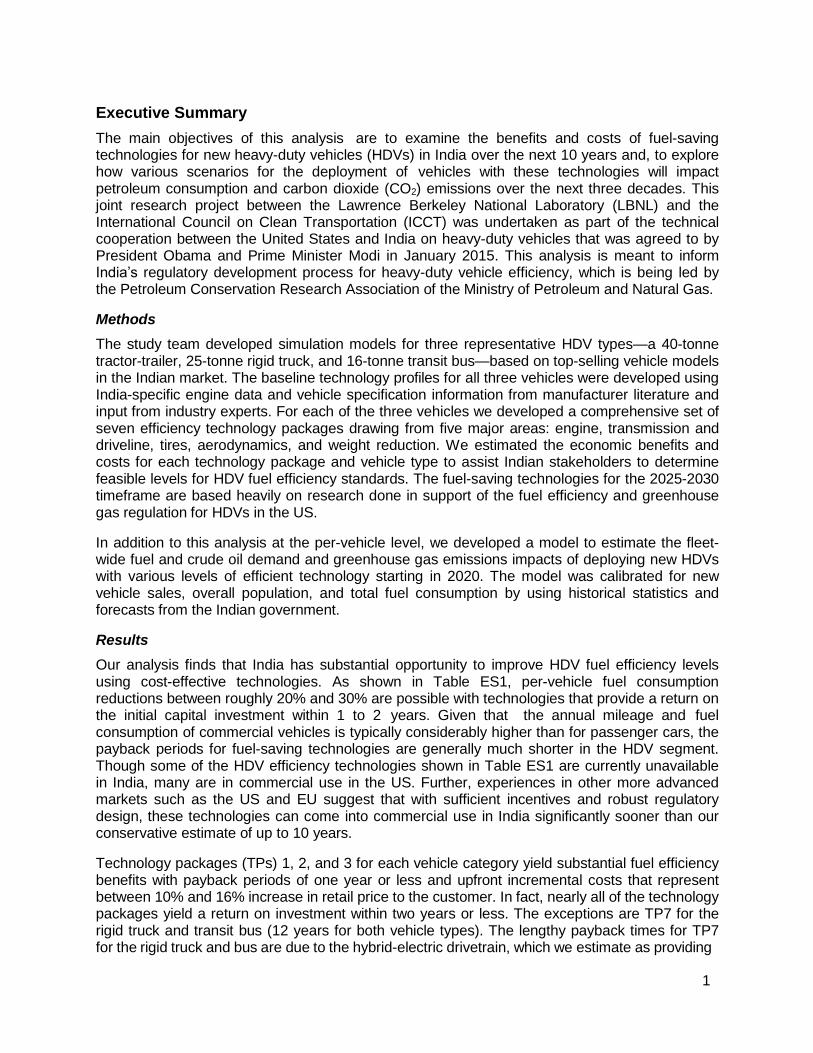
The main objectives of this analysis are to examine the benefits and costs of fuel-saving technologies for new heavy-duty vehicles (HDVs) in India over the next 10 years and, to explore how various scenarios for the deployment of vehicles with these technologies will impact petroleum consumption and carbon dioxide (CO2) emissions over the next three decades. This joint research project between the Lawrence Berkeley National Laboratory (LBNL) and the International Council on Clean Transportation (ICCT) was undertaken as part of the technical cooperation between the United States and India on heavy-duty vehicles that was agreed to by President Obama and Prime Minister Modi in January 2015. This analysis is meant to inform India’s regulatory development process for heavy-duty vehicle efficiency, which is being led by the Petroleum Conservation Research Association of the Ministry of Petroleum and Natural Gas.

Methods

The study team developed simulation models for three representative HDV types—a 40-tonne tractor-trailer, 25-tonne rigid truck, and 16-tonne transit bus—based on top-selling vehicle models in the Indian market. The baseline technology profiles for all three vehicles were developed using India-specific engine data and vehicle specification information from manufacturer literature and input from industry experts. For each of the three vehicles we developed a comprehensive set of seven efficiency technology packages drawing from five major areas: engine, transmission and driveline, tires, aerodynamics, and weight reduction. We estimated the economic benefits and costs for each technology package and vehicle type to assist Indian stakeholders to determine feasible levels for HDV fuel efficiency standards. The fuel-saving technologies for the 2025-2030 timeframe are based heavily on research done in support of the fuel efficiency and greenhouse gas regulation for HDVs in the US.

In addition to this analysis at the per-vehicle level, we developed a model to estimate the fleet- wide fuel and crude oil demand and greenhouse gas emissions impacts of deploying new HDVs with various levels of efficient technology starting in 2020. The model was calibrated for new vehicle sales, overall population, and total fuel consumption by using historical statistics and forecasts from the Indian government.

Results

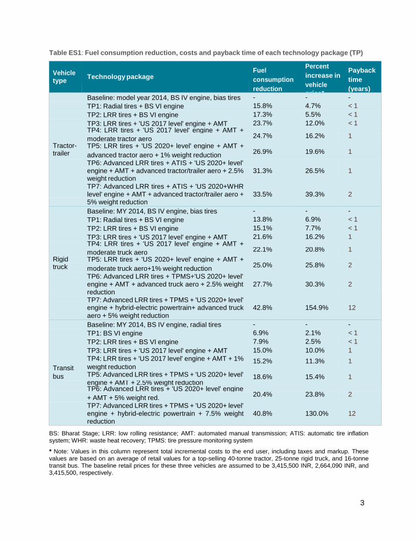
Our analysis finds that India has substantial opportunity to improve HDV fuel efficiency levels using cost-effective technologies. As shown in Table ES1, per-vehicle fuel consumption reductions between roughly 20% and 30% are possible with technologies that provide a return on the initial capital investment within 1 to 2 years. Given that the annual mileage and fuel consumption of commercial vehicles is typically considerably higher than for passenger cars, the payback periods for fuel-saving technologies are generally much shorter in the HDV segment. Though some of the HDV efficiency technologies shown in Table ES1 are currently unavailable in India, many are in commercial use in the US. Further, experiences in other more advanced markets such as the US and EU suggest that with sufficient incentives and robust regulatory design, these technologies can come into commercial use in India significantly sooner than our conservative estimate of up to 10 years.

Technology packages (TPs) 1, 2, and 3 for each vehicle category yield substantial fuel efficiency benefits with payback periods of one year or less and upfront incremental costs that represent between 10% and 16% increase in retail price to the customer. In fact, nearly all of the technology packages yield a return on investment within two years or less. The exceptions are TP7 for the rigid truck and transit bus (12 years for both vehicle types). The lengthy payback times for TP7 for the rigid truck and bus are due to the hybrid-electric drivetrain, which we estimate as providing

2

substantial fuel savings (20-25%), though the costs are significantly higher than any of the other technologies examined in this study. Importantly, when the incentive for hybrid buses under the FAME India scheme is included, the payback period drops to zero. In other words, the FAME incentive is large enough to eliminate the difference in cost between a hybrid bus and an equivalent conventional diesel bus.

Across all of the technology packages and vehicle types, engine and tire technologies provide the most cost-effective efficiency improvements. The high degree of cost-effectiveness for these two technology areas is primarily driven by two factors: 1) under India-specific driving conditions (i.e., low average speeds and large prevalence of over-loading), the combined energy losses due to the engine and tires represent between 75% and 85% of the total losses, and 2) engine and tire technologies are relatively inexpensive compared to advancements in other technology areas.

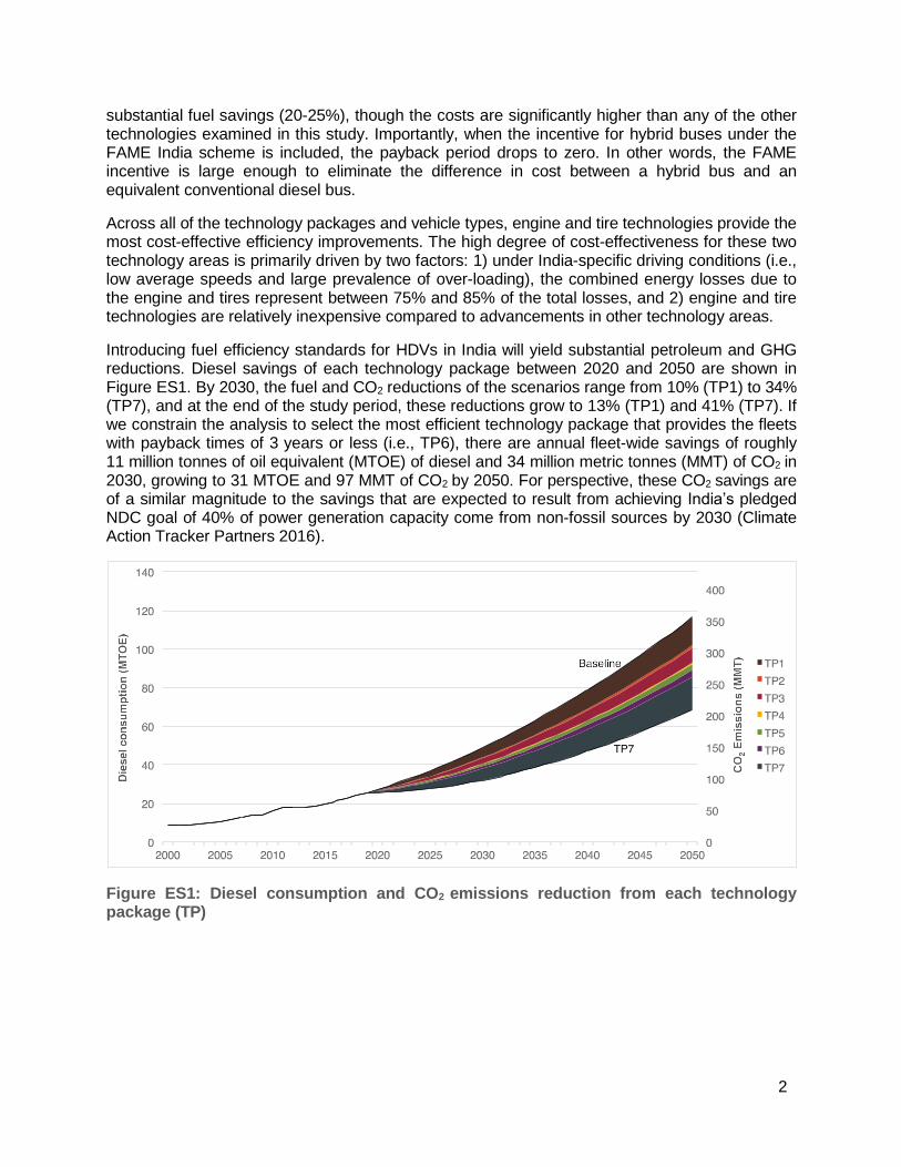
Introducing fuel efficiency standards for HDVs in India will yield substantial petroleum and GHG reductions. Diesel savings of each technology package between 2020 and 2050 are shown in Figure ES1. By 2030, the fuel and CO2 reductions of the scenarios range from 10% (TP1) to 34% (TP7), and at the end of the study period, these reductions grow to 13% (TP1) and 41% (TP7). If we constrain the analysis to select the most efficient technology package that provides the fleets with payback times of 3 years or less (i.e., TP6), there are annual fleet-wide savings of roughly 11 million tonnes of oil equivalent (MTOE) of diesel and 34 million metric tonnes (MMT) of CO2 in 2030, growing to 31 MTOE and 97 MMT of CO2 by 2050. For perspective, these CO2 savings are of a similar magnitude to the savings that are expected to result from achieving India’s pledged NDC goal of 40% of power generation capacity come from non-fossil sources by 2030 (Climate Action Tracker Partners 2016).

Figure ES1: Diesel consumption and CO2 emissions reduction from each technology package (TP)

3

Table ES1: Fuel consumption reduction, costs and payback time of each technology package (TP)

Vehicle type

Technology package

Fuel Percent

Payback

consumption increase in

time

reduction vehicle

(years) price*

Baseline: model year 2014, BS IV engine, bias tires - - -

TP1: Radial tires + BS VI engine 15.8% 4.7% < 1

TP2: LRR tires + BS VI engine 17.3% 5.5% < 1

TP3: LRR tires + 'US 2017 level' engine + AMT 23.7% 12.0% < 1

TP4: LRR tires + 'US 2017 level' engine + AMT + moderate tractor aero 24.7% 16.2% 1

Tractor- TP5: LRR tires + 'US 2020+ level' engine + AMT + trailer advanced tractor aero + 1% weight reduction 26.9% 19.6% 1

TP6: Advanced LRR tires + ATIS + 'US 2020+ level' engine + AMT + advanced tractor/trailer aero + 2.5% 31.3% 26.5% 1 weight reduction TP7: Advanced LRR tires + ATIS + 'US 2020+WHR level' engine + AMT + advanced tractor/trailer aero + 33.5% 39.3% 2 5% weight reduction Baseline: MY 2014, BS IV engine, bias tires - - -

TP1: Radial tires + BS VI engine 13.8% 6.9% < 1


TP3: LRR tires + 'US 2017 level' engine + AMT 21.6% 16.2% 1

TP4: LRR tires + 'US 2017 level' engine + AMT + moderate truck aero 22.1% 20.8% 1

Rigid TP5: LRR tires + 'US 2020+ level' engine + AMT + truck moderate truck aero+1% weight reduction 25.0% 25.8% 2

TP6: Advanced LRR tires + TPMS+'US 2020+ level' engine + AMT + advanced truck aero + 2.5% weight 27.7% 30.3% 2 reduction TP7: Advanced LRR tires + TPMS + 'US 2020+ level' engine + hybrid-electric powertrain+ advanced truck 42.8% 154.9% 12

aero + 5% weight reduction Baseline: MY 2014, BS IV engine, radial tires - - -

TP1: BS VI engine 6.9% 2.1% < 1


TP3: LRR tires + 'US 2017 level' engine + AMT 15.0% 10.0% 1

TP4: LRR tires + 'US 2017 level' engine + AMT + 1% 15.2% 11.3% 1 Transit weight reduction bus TP5: Advanced LRR tires + TPMS + 'US 2020+ level' 18.6% 15.4% 1

engine + AMT + 2.5% weight reduction TP6: Advanced LRR tires + 'US 2020+ level' engine + AMT + 5% weight red. 20.4% 23.8% 2

TP7: Advanced LRR tires + TPMS + 'US 2020+ level' engine + hybrid-electric powertrain + 7.5% weight 40.8% 130.0% 12 reduction

BS: Bharat Stage; LRR: low rolling resistance; AMT: automated manual transmission; ATIS: automatic tire inflation system; WHR: waste heat recovery; TPMS: tire pressure monitoring system

* Note: Values in this column represent total incremental costs to the end user, including taxes and markup. These values are based on an average of retail values for a top-selling 40-tonne tractor, 25-tonne rigid truck, and 16-tonne transit bus. The baseline retail prices for these three vehicles are assumed to be 3,415,500 INR, 2,664,090 INR, and 3,415,500, respectively.

4

Recommendations

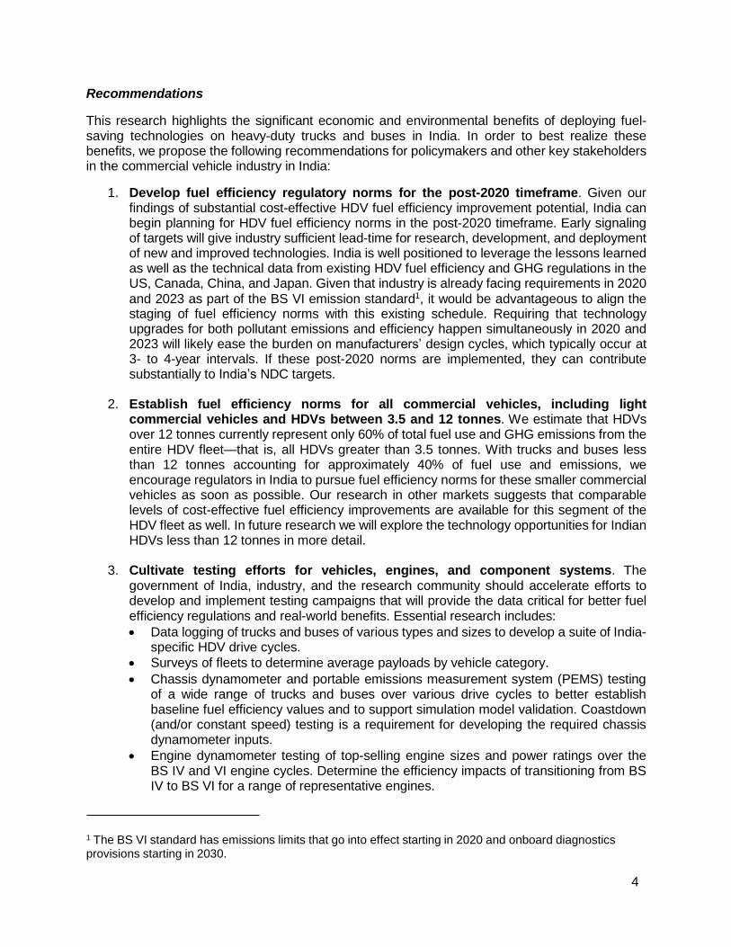
This research highlights the significant economic and environmental benefits of deploying fuel- saving technologies on heavy-duty trucks and buses in India. In order to best realize these benefits, we propose the following recommendations for policymakers and other key stakeholders in the commercial vehicle industry in India:

1. Develop fuel efficiency regulatory norms for the post-2020 timeframe. Given our findings of substantial cost-effective HDV fuel efficiency improvement potential, India can begin planning for HDV fuel efficiency norms in the post-2020 timeframe. Early signaling of targets will give industry sufficient lead-time for research, development, and deployment of new and improved technologies. India is well positioned to leverage the lessons learned as well as the technical data from existing HDV fuel efficiency and GHG regulations in the US, Canada, China, and Japan. Given that industry is already facing requirements in 2020

and 2023 as part of the BS VI emission standard1, it would be advantageous to align the staging of fuel efficiency norms with this existing schedule. Requiring that technology upgrades for both pollutant emissions and efficiency happen simultaneously in 2020 and 2023 will likely ease the burden on manufacturers’ design cycles, which typically occur at 3- to 4-year intervals. If these post-2020 norms are implemented, they can contribute substantially to India’s NDC targets.

2. Establish fuel efficiency norms for all commercial vehicles, including light commercial vehicles and HDVs between 3.5 and 12 tonnes. We estimate that HDVs over 12 tonnes currently represent only 60% of total fuel use and GHG emissions from the entire HDV fleet—that is, all HDVs greater than 3.5 tonnes. With trucks and buses less than 12 tonnes accounting for approximately 40% of fuel use and emissions, we encourage regulators in India to pursue fuel efficiency norms for these smaller commercial vehicles as soon as possible. Our research in other markets suggests that comparable levels of cost-effective fuel efficiency improvements are available for this segment of the HDV fleet as well. In future research we will explore the technology opportunities for Indian HDVs less than 12 tonnes in more detail.

3. Cultivate testing efforts for vehicles, engines, and component systems. The government of India, industry, and the research community should accelerate efforts to develop and implement testing campaigns that will provide the data critical for better fuel efficiency regulations and real-world benefits. Essential research includes:

Data logging of trucks and buses of various types and sizes to develop a suite of India- specific HDV drive cycles.

Surveys of fleets to determine average payloads by vehicle category.

Chassis dynamometer and portable emissions measurement system (PEMS) testing of a wide range of trucks and buses over various drive cycles to better establish baseline fuel efficiency values and to support simulation model validation. Coastdown (and/or constant speed) testing is a requirement for developing the required chassis dynamometer inputs.

Engine dynamometer testing of top-selling engine sizes and power ratings over the BS IV and VI engine cycles. Determine the efficiency impacts of transitioning from BS IV to BS VI for a range of representative engines.

1 The BS VI standard has emissions limits that go into effect starting in 2020 and onboard diagnostics provisions starting in 2030.

5

Testing of a broad range of bias and radial tires for rolling resistance and wet grip performance.

6

1 Introduction

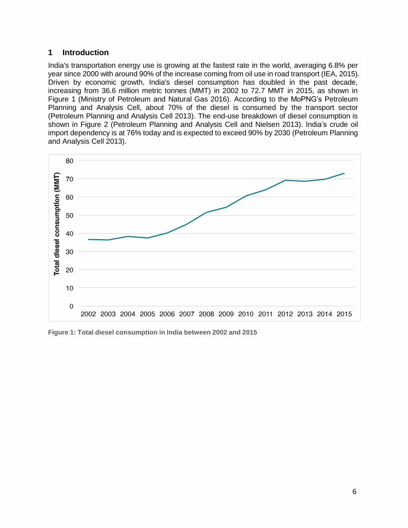
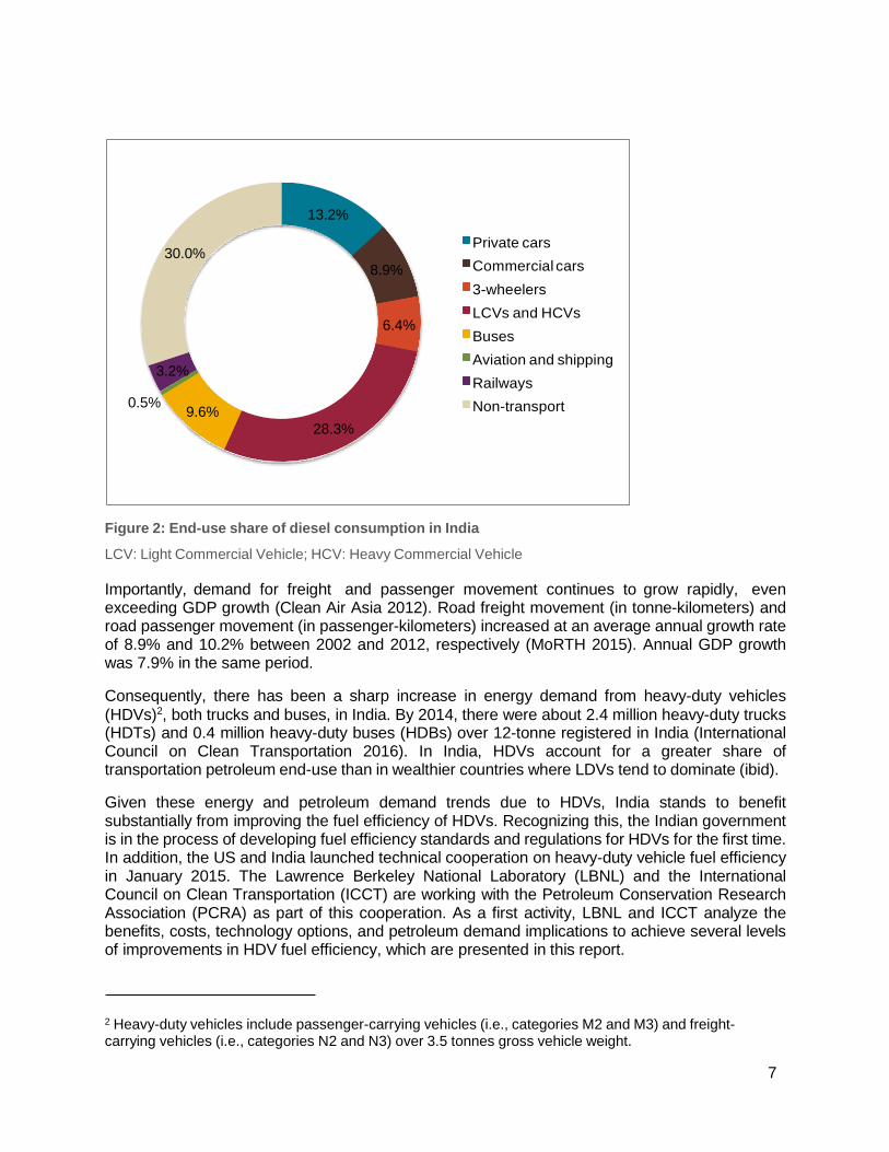
India's transportation energy use is growing at the fastest rate in the world, averaging 6.8% per year since 2000 with around 90% of the increase coming from oil use in road transport (IEA, 2015). Driven by economic growth, India's diesel consumption has doubled in the past decade, increasing from 36.6 million metric tonnes (MMT) in 2002 to 72.7 MMT in 2015, as shown in Figure 1 (Ministry of Petroleum and Natural Gas 2016). According to the MoPNG’s Petroleum Planning and Analysis Cell, about 70% of the diesel is consumed by the transport sector (Petroleum Planning and Analysis Cell 2013). The end-use breakdown of diesel consumption is shown in Figure 2 (Petroleum Planning and Analysis Cell and Nielsen 2013). India’s crude oil import dependency is at 76% today and is expected to exceed 90% by 2030 (Petroleum Planning and Analysis Cell 2013).

Figure 1: Total diesel consumption in India between 2002 and 2015

7

Figure 2: End-use share of diesel consumption in India

LCV: Light Commercial Vehicle; HCV: Heavy Commercial Vehicle

Importantly, demand for freight and passenger movement continues to grow rapidly, even exceeding GDP growth (Clean Air Asia 2012). Road freight movement (in tonne-kilometers) and road passenger movement (in passenger-kilometers) increased at an average annual growth rate of 8.9% and 10.2% between 2002 and 2012, respectively (MoRTH 2015). Annual GDP growth was 7.9% in the same period.

Consequently, there has been a sharp increase in energy demand from heavy-duty vehicles

(HDVs)2, both trucks and buses, in India. By 2014, there were about 2.4 million heavy-duty trucks (HDTs) and 0.4 million heavy-duty buses (HDBs) over 12-tonne registered in India (International Council on Clean Transportation 2016). In India, HDVs account for a greater share of transportation petroleum end-use than in wealthier countries where LDVs tend to dominate (ibid).

Given these energy and petroleum demand trends due to HDVs, India stands to benefit substantially from improving the fuel efficiency of HDVs. Recognizing this, the Indian government is in the process of developing fuel efficiency standards and regulations for HDVs for the first time. In addition, the US and India launched technical cooperation on heavy-duty vehicle fuel efficiency in January 2015. The Lawrence Berkeley National Laboratory (LBNL) and the International Council on Clean Transportation (ICCT) are working with the Petroleum Conservation Research Association (PCRA) as part of this cooperation. As a first activity, LBNL and ICCT analyze the benefits, costs, technology options, and petroleum demand implications to achieve several levels of improvements in HDV fuel efficiency, which are presented in this report.

2 Heavy-duty vehicles include passenger-carrying vehicles (i.e., categories M2 and M3) and freight- carrying vehicles (i.e., categories N2 and N3) over 3.5 tonnes gross vehicle weight.

13.2%

30.0% 8.9%

6.4%

3.2%

0.5% 9.6%

Private cars

Commercial cars

3-wheelers

LCVs and HCVs

Buses

Aviation and shipping

Railways

Non-transport

28.3%

8

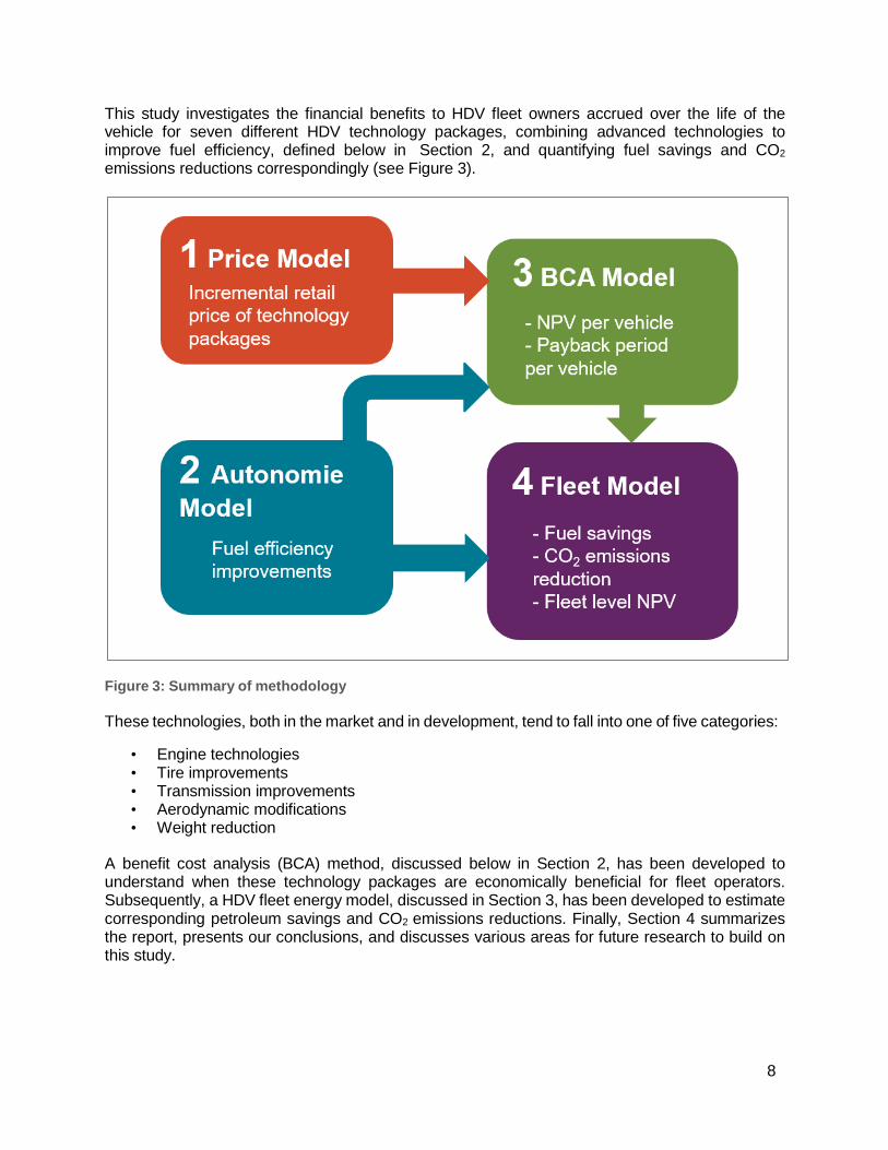
This study investigates the financial benefits to HDV fleet owners accrued over the life of the vehicle for seven different HDV technology packages, combining advanced technologies to improve fuel efficiency, defined below in Section 2, and quantifying fuel savings and CO2

emissions reductions correspondingly (see Figure 3).

Figure 3: Summary of methodology

These technologies, both in the market and in development, tend to fall into one of five categories:

• Engine technologies • Tire improvements • Transmission improvements • Aerodynamic modifications • Weight reduction

A benefit cost analysis (BCA) method, discussed below in Section 2, has been developed to understand when these technology packages are economically beneficial for fleet operators. Subsequently, a HDV fleet energy model, discussed in Section 3, has been developed to estimate corresponding petroleum savings and CO2 emissions reductions. Finally, Section 4 summarizes the report, presents our conclusions, and discusses various areas for future research to build on this study.

9

2 Benefit cost analysis

This section describes the representative vehicle models and technology areas that were explored in this analysis. After discussing the baseline vehicle technology levels and the methods utilized to project the future opportunities for efficiency technologies, we estimate the fuel consumption reduction potential for seven technology packages for three HDV types. Finally, we perform a comprehensive assessment of the costs and benefits associated with each of these technology packages.

2.1 Vehicle classes and technology packages

The primary objective of this paper is to estimate the efficiency gains from technologies that will be available over the next 10 years for HDVs in India and how various scenarios for the deployment of these fuel-saving technologies will impact fleet-wide fuel consumption and costs. This section describes our methodology for developing baseline technology levels and a set of increasingly fuel efficient technology packages for three representative HDV types: a tractor truck, rigid truck, and transit bus. In addition, we provide per-vehicle cost estimates for each of the technologies and technology packages.

In this paper, the term ‘tractor’ and ‘tractor truck’ are used interchangeably to represent an articulated freight truck that can haul a cargo-carrying trailer, which can be detached from the truck chassis. Rigid truck includes all other non-articulated freight trucks in which the cargo- carrying body is permanently attached to the truck chassis. Transit bus refers to buses that primarily operate within cities on fixed routes.

For this analysis, we developed vehicle simulation models for three representative HDV types based on popular models in the Indian market. Each of these three representative vehicles is modeled using data on vehicle characteristics from a sales database that we acquired for fiscal year 2013-2014. Based on that sales market database, the HDV models that we chose to analyze were specified in the simulation tool to resemble the top-selling models in their respective vehicle

segments.3

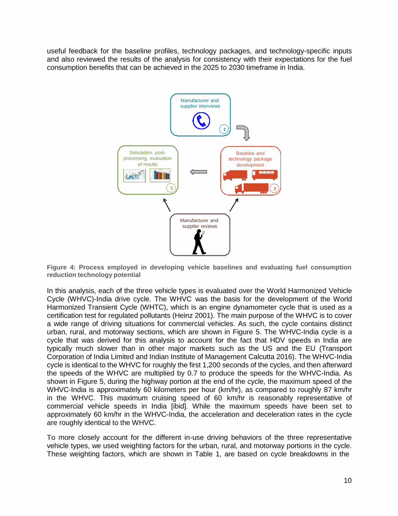
Figure 4 shows the process that was utilized to establish and verify the baseline vehicle models, develop a set of technology packages, and estimate the fuel consumption reduction potential of each of these technology packages. As shown, the first step involved a number of interviews with some of the leading component suppliers in the HDV market in India. All three of the companies expressed a preference for anonymity. Without revealing any specifics, each company has a sizable market share of the HDV engine, transmission, and tire sales, respectively. For each of the three vehicle types, these suppliers were able to provide valuable insights on the current state of technology and what advances are reasonably possible over the next 10 years in India. Using the responses from suppliers as well as information available from manufacturer data sheets, we assembled baseline profiles and a set of technology packages with increasing levels of fuel- saving technologies, as described in the subsequent section. In the final step, we simulated each of the technology packages in Autonomie, which is a vehicle performance evaluation software platform that was developed by the US Department of Energy’s Argonne National Laboratory (UChicago Argonne LLC 2016). Due to resource constraints, we were unable to model improvements in certain systems such as the transmission and driveline, so the fuel consumption benefits of advancements in these technology areas were accounted for in the post-processing of the simulation results. Throughout the study, our component manufacturer colleagues provided

3 For a more in-depth study of the Indian HDV market, see: http://www.theicct.org/market-analysis-heavy- duty-vehicles-india

http://www.theicct.org/market-analysis-heavy-duty-vehicles-india

http://www.theicct.org/market-analysis-heavy-duty-vehicles-india

10

Simulation, post- processing, evaluation

of results Tract or-trail er

100% 80

84% 83%

9

0%

80

%

7

0

%

6

0

%

5

0%

4

0%

30

%

2

0

%

1

0%

0

%

76%

75%

74%

7

0

60

68%

65% 50

4

0

30

10

0

T ime ( s econds) 1 2 3 4

5 6 7 8

Package number WH VC WH VC -I nd i a

3

useful feedback for the baseline profiles, technology packages, and technology-specific inputs and also reviewed the results of the analysis for consistency with their expectations for the fuel consumption benefits that can be achieved in the 2025 to 2030 timeframe in India.

Figure 4: Process employed in developing vehicle baselines and evaluating fuel consumption reduction technology potential

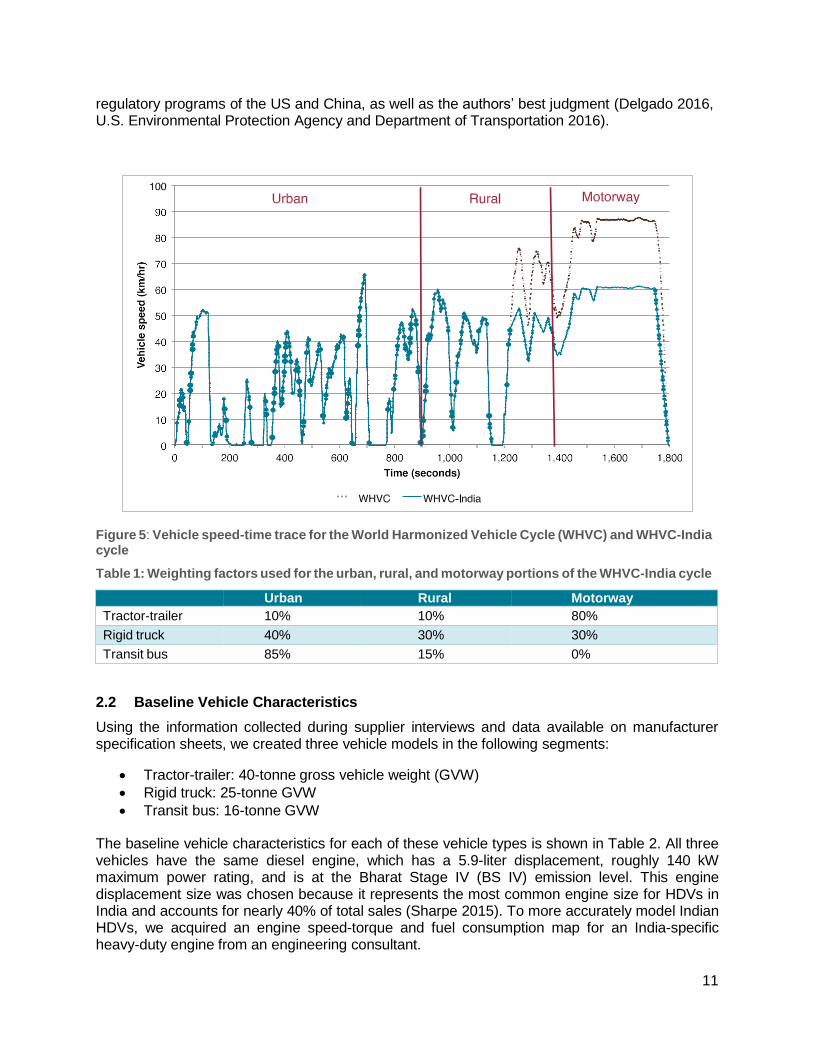
In this analysis, each of the three vehicle types is evaluated over the World Harmonized Vehicle Cycle (WHVC)-India drive cycle. The WHVC was the basis for the development of the World Harmonized Transient Cycle (WHTC), which is an engine dynamometer cycle that is used as a certification test for regulated pollutants (Heinz 2001). The main purpose of the WHVC is to cover a wide range of driving situations for commercial vehicles. As such, the cycle contains distinct urban, rural, and motorway sections, which are shown in Figure 5. The WHVC-India cycle is a cycle that was derived for this analysis to account for the fact that HDV speeds in India are typically much slower than in other major markets such as the US and the EU (Transport Corporation of India Limited and Indian Institute of Management Calcutta 2016). The WHVC-India cycle is identical to the WHVC for roughly the first 1,200 seconds of the cycles, and then afterward the speeds of the WHVC are multiplied by 0.7 to produce the speeds for the WHVC-India. As shown in Figure 5, during the highway portion at the end of the cycle, the maximum speed of the WHVC-India is approximately 60 kilometers per hour (km/hr), as compared to roughly 87 km/hr in the WHVC. This maximum cruising speed of 60 km/hr is reasonably representative of commercial vehicle speeds in India [ibid]. While the maximum speeds have been set to approximately 60 km/hr in the WHVC-India, the acceleration and deceleration rates in the cycle are roughly identical to the WHVC.

To more closely account for the different in-use driving behaviors of the three representative vehicle types, we used weighting factors for the urban, rural, and motorway portions in the cycle. These weighting factors, which are shown in Table 1, are based on cycle breakdowns in the

Manufacturer and

supplier reviews

Baseline and technology package

development

2

Manufacturer and supplier interviews

1

Ve

hic

le

sp

ee

d

(km

/hr)

fu

el

co

ns

um

ptio

n

re

du

ctio

n

vs

. B

as

elin

e

11

regulatory programs of the US and China, as well as the authors’ best judgment (Delgado 2016, U.S. Environmental Protection Agency and Department of Transportation 2016).

Figure 5: Vehicle speed-time trace for the World Harmonized Vehicle Cycle (WHVC) and WHVC-India cycle

Table 1: Weighting factors used for the urban, rural, and motorway portions of the WHVC-India cycle

Urban Rural Motorway Tractor-trailer 10% 10% 80%

Rigid truck 40% 30% 30%

Transit bus 85% 15% 0%

2.2 Baseline Vehicle Characteristics

Using the information collected during supplier interviews and data available on manufacturer specification sheets, we created three vehicle models in the following segments:

Tractor-trailer: 40-tonne gross vehicle weight (GVW)

Rigid truck: 25-tonne GVW

Transit bus: 16-tonne GVW

The baseline vehicle characteristics for each of these vehicle types is shown in Table 2. All three vehicles have the same diesel engine, which has a 5.9-liter displacement, roughly 140 kW maximum power rating, and is at the Bharat Stage IV (BS IV) emission level. This engine displacement size was chosen because it represents the most common engine size for HDVs in India and accounts for nearly 40% of total sales (Sharpe 2015). To more accurately model Indian HDVs, we acquired an engine speed-torque and fuel consumption map for an India-specific heavy-duty engine from an engineering consultant.

12

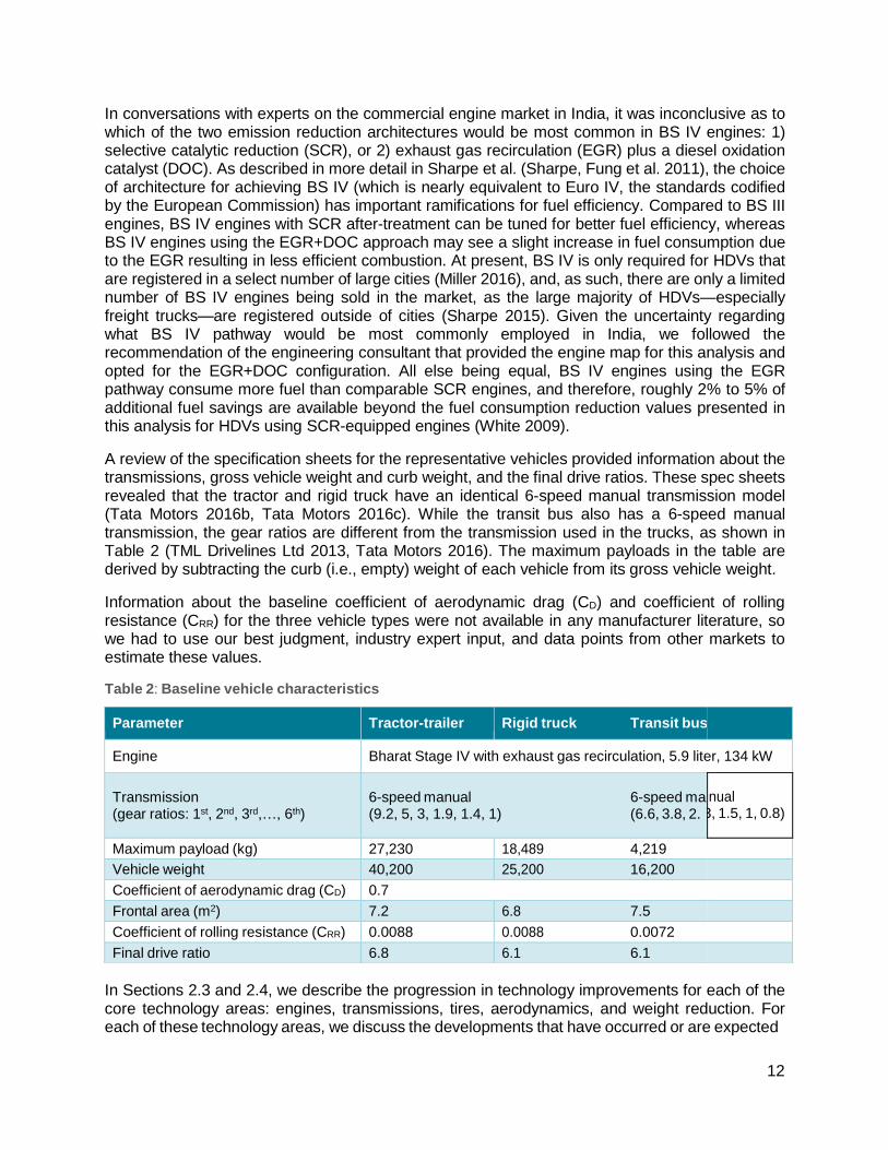
In conversations with experts on the commercial engine market in India, it was inconclusive as to which of the two emission reduction architectures would be most common in BS IV engines: 1) selective catalytic reduction (SCR), or 2) exhaust gas recirculation (EGR) plus a diesel oxidation catalyst (DOC). As described in more detail in Sharpe et al. (Sharpe, Fung et al. 2011), the choice of architecture for achieving BS IV (which is nearly equivalent to Euro IV, the standards codified by the European Commission) has important ramifications for fuel efficiency. Compared to BS III engines, BS IV engines with SCR after-treatment can be tuned for better fuel efficiency, whereas BS IV engines using the EGR+DOC approach may see a slight increase in fuel consumption due to the EGR resulting in less efficient combustion. At present, BS IV is only required for HDVs that are registered in a select number of large cities (Miller 2016), and, as such, there are only a limited number of BS IV engines being sold in the market, as the large majority of HDVs—especially freight trucks—are registered outside of cities (Sharpe 2015). Given the uncertainty regarding what BS IV pathway would be most commonly employed in India, we followed the recommendation of the engineering consultant that provided the engine map for this analysis and opted for the EGR+DOC configuration. All else being equal, BS IV engines using the EGR pathway consume more fuel than comparable SCR engines, and therefore, roughly 2% to 5% of additional fuel savings are available beyond the fuel consumption reduction values presented in this analysis for HDVs using SCR-equipped engines (White 2009).

A review of the specification sheets for the representative vehicles provided information about the transmissions, gross vehicle weight and curb weight, and the final drive ratios. These spec sheets revealed that the tractor and rigid truck have an identical 6-speed manual transmission model (Tata Motors 2016b, Tata Motors 2016c). While the transit bus also has a 6-speed manual transmission, the gear ratios are different from the transmission used in the trucks, as shown in Table 2 (TML Drivelines Ltd 2013, Tata Motors 2016). The maximum payloads in the table are derived by subtracting the curb (i.e., empty) weight of each vehicle from its gross vehicle weight.

Information about the baseline coefficient of aerodynamic drag (CD) and coefficient of rolling resistance (CRR) for the three vehicle types were not available in any manufacturer literature, so we had to use our best judgment, industry expert input, and data points from other markets to estimate these values.

Table 2: Baseline vehicle characteristics

nual 3, 1.5, 1, 0.8)

In Sections 2.3 and 2.4, we describe the progression in technology improvements for each of the core technology areas: engines, transmissions, tires, aerodynamics, and weight reduction. For each of these technology areas, we discuss the developments that have occurred or are expected

Parameter Tractor-trailer Rigid truck Transit bus

Engine Bharat Stage IV with exhaust gas recirculation, 5.9 liter, 134 kW

Transmission (gear ratios: 1st, 2nd, 3rd,…, 6th)

6-speed manual 6-speed ma (9.2, 5, 3, 1.9, 1.4, 1) (6.6, 3.8, 2.

Maximum payload (kg) 27,230 18,489 4,219 Vehicle weight 40,200 25,200 16,200

Coefficient of aerodynamic drag (CD) 0.7

Frontal area (m2) 7.2 6.8 7.5

Coefficient of rolling resistance (CRR) 0.0088 0.0088 0.0072

Final drive ratio 6.8 6.1 6.1

13

to occur in the more advanced markets of the US and the EU over the next 10-15 years in terms of the technology pathways that are most applicable in the Indian context. We then outline how the progressions in technology cascade through each of the seven technology packages from the baseline for each vehicle type.

2.3 Powertrain technologies

Sections 2.3.1 and 2.3.2 describe the fuel-saving technologies that were investigated for the engine and transmission.

2.3.1 Engine technologies

Starting in 2000, India implemented emission standards for HDVs that were harmonized with the Euro regulatory pathway (Central Pollution Control Board 2008). With Bharat Stage IV (BS IV) emissions standards going into effect nationwide starting in model year 2017, this was the assumed baseline level for engine technology. As discussed in more detail in Sharpe and Delgado (2016), the transition from BS III to IV in diesel engines involves the introduction of electronically- controlled common rail fuel injection at increased pressure (typically around 1,600 bar), improved combustion and calibration for particulate matter (PM) control, turbocharging with intercooling, as well as improvements to other engine systems.

In early 2016, the Ministry of Road Transport and Highways issued a draft notification of leapfrogging BS V to go directly to BS VI emission standards for all major on-road vehicle categories in India (The Gazette of India 2016). As proposed, the BS VI standards will go into effect for all HDVs manufactured on or after April 1, 2020. The shift from BS III to IV to VI is going to require that manufacturers invest in a number of technologies to achieve the target brake- specific levels of nitrogen oxides (NOx) and PM emissions. The most significant technology addition in the transition to BS VI is the introduction of diesel particular filters (DPFs) for PM control. In bringing down PM to very low levels, DPFs impact the fuel consumption of an engine in a number of ways. Comparing BS IV to VI engines (which, in this analysis, is assumed to be equivalent to comparing Euro IV to VI), the fuel usage rates of an engine are negatively impacted with the introduction of DPFs by up to 2-3%, though efficiency improvements to various other areas of the engine result in a net reduction in fuel consumption (Sharpe, Fung et al. 2011, Sharpe and Delgado 2016). For this study, we assume that BS VI engines consume 5% less fuel than comparable BS IV engines based on the available literature and our best judgment.

Table 3 shows the three additional steps in engine technology advancement beyond BS VI assumed in this analysis. These levels of engine efficiency improvements borrow from the methodology employed in Delgado and Lutsey (2015), and based on interview responses from industry experts in India, we assume that roughly comparable engine technologies can be employed in the India HDV market. These engine technology areas include:

Friction reduction

On-demand accessories

Combustion system optimization

Advanced engine controls

After-treatment improvements

Turbocharger improvements

Waste heat recovery (WHR) systems, including turbocompounding and Rankine bottoming cycles

14

The percentage reduction in fuel consumption values in Table 3 are approximations based on the Delgado and Lutsey study (Delgado and Lutsey 2015). Delgado and Lutsey assume a US model year 2010 baseline, which is roughly equivalent to a BS VI (or Euro VI) engine, as both emission levels require nearly the same emissions control technologies that achieve about the same emission benefits (Sharpe and Delgado 2016). The Delgado and Lutsey analysis is centered around tractor-trailers, but we assume that similar levels of engine improvements are applicable for rigid trucks and transit buses, though the specific technology pathways vary based on differences in load and duty cycle. Roughly equivalent levels of fuel efficiency technology potential have been evidenced in engines across the various HDV classes in the US regulatory program (US Environmental Protection Agency and Department of Transportation 2016).

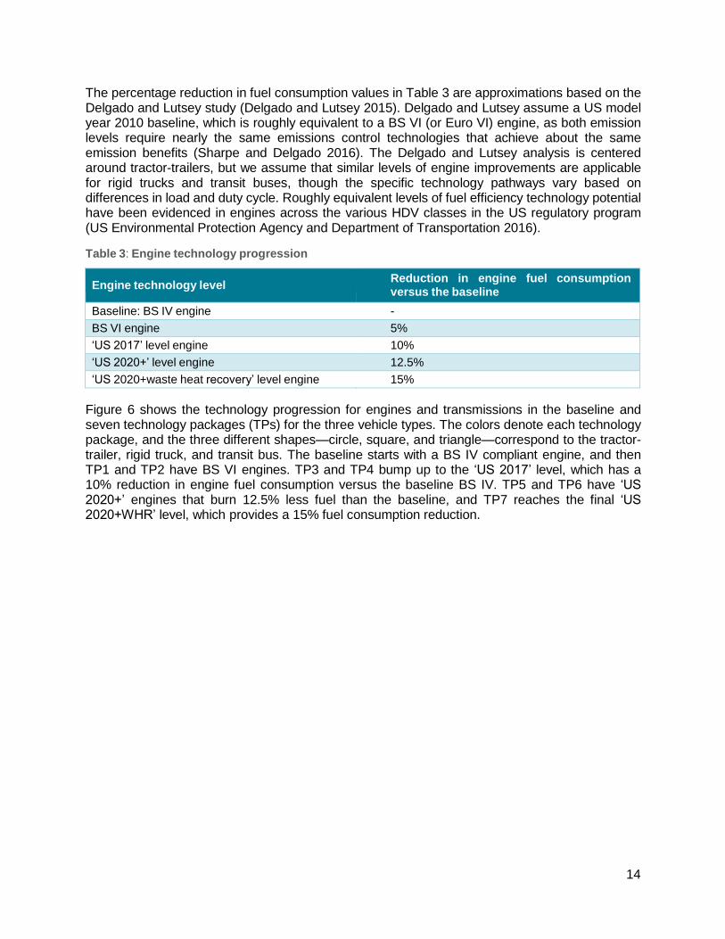
Table 3: Engine technology progression

Engine technology level Reduction in engine fuel consumption versus the baseline

Baseline: BS IV engine -

BS VI engine 5%

‘US 2017’ level engine 10%

‘US 2020+’ level engine 12.5%

‘US 2020+waste heat recovery’ level engine 15%

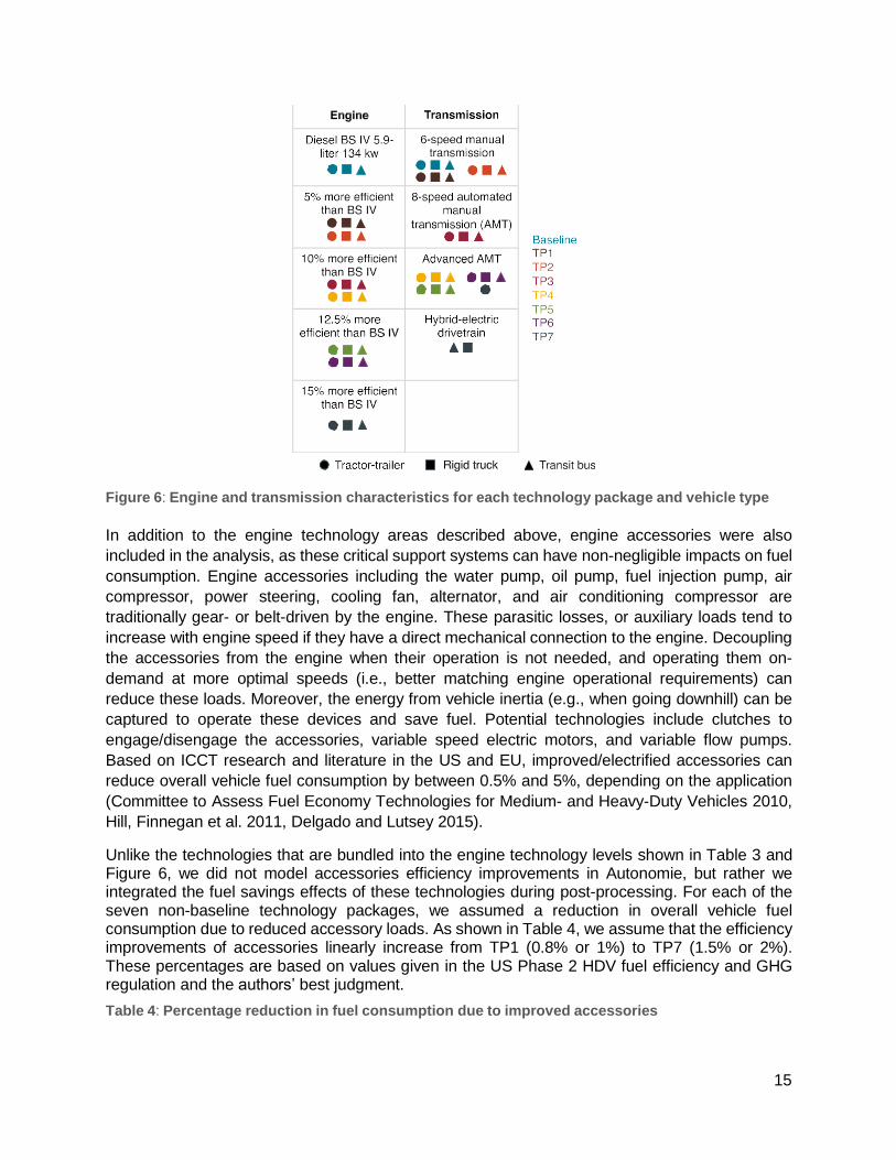
Figure 6 shows the technology progression for engines and transmissions in the baseline and seven technology packages (TPs) for the three vehicle types. The colors denote each technology package, and the three different shapes—circle, square, and triangle—correspond to the tractor- trailer, rigid truck, and transit bus. The baseline starts with a BS IV compliant engine, and then TP1 and TP2 have BS VI engines. TP3 and TP4 bump up to the ‘US 2017’ level, which has a 10% reduction in engine fuel consumption versus the baseline BS IV. TP5 and TP6 have ‘US 2020+’ engines that burn 12.5% less fuel than the baseline, and TP7 reaches the final ‘US 2020+WHR’ level, which provides a 15% fuel consumption reduction.

15

Figure 6: Engine and transmission characteristics for each technology package and vehicle type

In addition to the engine technology areas described above, engine accessories were also

included in the analysis, as these critical support systems can have non-negligible impacts on fuel

consumption. Engine accessories including the water pump, oil pump, fuel injection pump, air

compressor, power steering, cooling fan, alternator, and air conditioning compressor are

traditionally gear- or belt-driven by the engine. These parasitic losses, or auxiliary loads tend to

increase with engine speed if they have a direct mechanical connection to the engine. Decoupling

the accessories from the engine when their operation is not needed, and operating them on-

demand at more optimal speeds (i.e., better matching engine operational requirements) can

reduce these loads. Moreover, the energy from vehicle inertia (e.g., when going downhill) can be

captured to operate these devices and save fuel. Potential technologies include clutches to

engage/disengage the accessories, variable speed electric motors, and variable flow pumps.

Based on ICCT research and literature in the US and EU, improved/electrified accessories can

reduce overall vehicle fuel consumption by between 0.5% and 5%, depending on the application

(Committee to Assess Fuel Economy Technologies for Medium- and Heavy-Duty Vehicles 2010,

Hill, Finnegan et al. 2011, Delgado and Lutsey 2015).

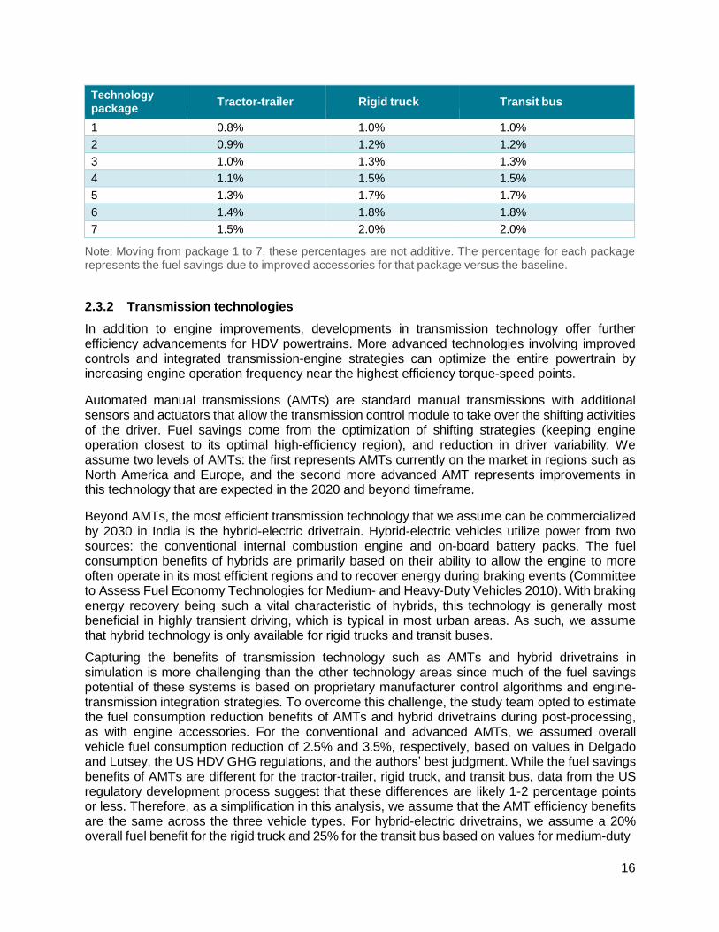
Unlike the technologies that are bundled into the engine technology levels shown in Table 3 and Figure 6, we did not model accessories efficiency improvements in Autonomie, but rather we integrated the fuel savings effects of these technologies during post-processing. For each of the seven non-baseline technology packages, we assumed a reduction in overall vehicle fuel consumption due to reduced accessory loads. As shown in Table 4, we assume that the efficiency improvements of accessories linearly increase from TP1 (0.8% or 1%) to TP7 (1.5% or 2%). These percentages are based on values given in the US Phase 2 HDV fuel efficiency and GHG regulation and the authors’ best judgment.

Table 4: Percentage reduction in fuel consumption due to improved accessories

16

Technology package

Tractor-trailer Rigid truck Transit bus

1 0.8% 1.0% 1.0%

2 0.9% 1.2% 1.2%

3 1.0% 1.3% 1.3%

4 1.1% 1.5% 1.5%

5 1.3% 1.7% 1.7%

6 1.4% 1.8% 1.8%

7 1.5% 2.0% 2.0%

Note: Moving from package 1 to 7, these percentages are not additive. The percentage for each package represents the fuel savings due to improved accessories for that package versus the baseline.

2.3.2 Transmission technologies

In addition to engine improvements, developments in transmission technology offer further efficiency advancements for HDV powertrains. More advanced technologies involving improved controls and integrated transmission-engine strategies can optimize the entire powertrain by increasing engine operation frequency near the highest efficiency torque-speed points.

Automated manual transmissions (AMTs) are standard manual transmissions with additional sensors and actuators that allow the transmission control module to take over the shifting activities of the driver. Fuel savings come from the optimization of shifting strategies (keeping engine operation closest to its optimal high-efficiency region), and reduction in driver variability. We assume two levels of AMTs: the first represents AMTs currently on the market in regions such as North America and Europe, and the second more advanced AMT represents improvements in this technology that are expected in the 2020 and beyond timeframe.

Beyond AMTs, the most efficient transmission technology that we assume can be commercialized by 2030 in India is the hybrid-electric drivetrain. Hybrid-electric vehicles utilize power from two sources: the conventional internal combustion engine and on-board battery packs. The fuel consumption benefits of hybrids are primarily based on their ability to allow the engine to more often operate in its most efficient regions and to recover energy during braking events (Committee to Assess Fuel Economy Technologies for Medium- and Heavy-Duty Vehicles 2010). With braking energy recovery being such a vital characteristic of hybrids, this technology is generally most beneficial in highly transient driving, which is typical in most urban areas. As such, we assume that hybrid technology is only available for rigid trucks and transit buses.

Capturing the benefits of transmission technology such as AMTs and hybrid drivetrains in simulation is more challenging than the other technology areas since much of the fuel savings potential of these systems is based on proprietary manufacturer control algorithms and engine- transmission integration strategies. To overcome this challenge, the study team opted to estimate the fuel consumption reduction benefits of AMTs and hybrid drivetrains during post-processing, as with engine accessories. For the conventional and advanced AMTs, we assumed overall vehicle fuel consumption reduction of 2.5% and 3.5%, respectively, based on values in Delgado and Lutsey, the US HDV GHG regulations, and the authors’ best judgment. While the fuel savings benefits of AMTs are different for the tractor-trailer, rigid truck, and transit bus, data from the US regulatory development process suggest that these differences are likely 1-2 percentage points or less. Therefore, as a simplification in this analysis, we assume that the AMT efficiency benefits are the same across the three vehicle types. For hybrid-electric drivetrains, we assume a 20% overall fuel benefit for the rigid truck and 25% for the transit bus based on values for medium-duty

17

urban vehicles in the US Phase 2 rule (US Environmental Protection Agency and Department of Transportation 2016).

As shown in Figure 6, the transmission technology assumptions in this analysis are the same across the three vehicle types for Packages 1 through 6, and in Package 7, the rigid truck and transit bus have a hybrid-electric drivetrain, while the tractor-trailer retains the advanced AMT.

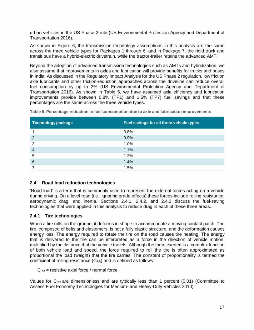
Beyond the adoption of advanced transmission technologies such as AMTs and hybridization, we also assume that improvements in axles and lubrication will provide benefits for trucks and buses in India. As discussed in the Regulatory Impact Analysis for the US Phase 2 regulation, low friction axle lubricants and other friction-reduction approaches across the driveline can reduce overall fuel consumption by up to 2% (US Environmental Protection Agency and Department of Transportation 2016). As shown in Table 5, we have assumed axle efficiency and lubrication improvements provide between 0.8% (TP1) and 1.5% (TP7) fuel savings and that these percentages are the same across the three vehicle types.

Table 5: Percentage reduction in fuel consumption due to axle and lubrication improvements

Technology package Fuel savings for all three vehicle types

1 0.8%

2 0.9%

3 1.0%

4 1.1%

5 1.3%

6 1.4%

7 1.5%

2.4 Road load reduction technologies

‘Road load’ is a term that is commonly used to represent the external forces acting on a vehicle during driving. On a level road (i.e., ignoring grade effects) these forces include rolling resistance, aerodynamic drag, and inertia. Sections 2.4.1, 2.4.2, and 2.4.3 discuss the fuel-saving technologies that were applied in this analysis to reduce drag in each of these three areas.

2.4.1 Tire technologies

When a tire rolls on the ground, it deforms in shape to accommodate a moving contact patch. The tire, composed of belts and elastomers, is not a fully elastic structure, and the deformation causes energy loss. The energy required to rotate the tire on the road causes tire heating. The energy that is delivered to the tire can be interpreted as a force in the direction of vehicle motion, multiplied by the distance that the vehicle travels. Although the force exerted is a complex function of both vehicle load and speed, the force required to roll the tire is often approximated as proportional the load (weight) that the tire carries. The constant of proportionality is termed the coefficient of rolling resistance (CRR) and is defined as follows:

CRR = resistive axial force / normal force Values for CRR are dimensionless and are typically less than 1 percent (0.01) (Committee to Assess Fuel Economy Technologies for Medium- and Heavy-Duty Vehicles 2010).

18

There are two broad categories of tire construction: bias and radial. A bias tire consists of multiple rubber plies overlapping each other, and the crown and sidewalls are interdependent. The overlapped plies form a thick layer that is less flexible and more sensitive to overheating. In radial tires, the casing ply runs perpendicular to the circumference of the tire, thereby increasing the flexibility of tires. Inextensible layers (belts) are placed underneath the tread in order to improve fuel efficiency and comfort during driving. In general, the most significant advantage of bias tires is that they are less expensive. On the other hand, radial tires tend to have longer useful life and yield better fuel efficiency and performance. From interviews with a number of tire suppliers, vehicle manufacturers, and fleets, bias tires make up roughly 80% of the HDV market in India (Malik, Karpate et al. 2016). According to industry experts, the continued dominance of bias tires is driven primary by the cost sensitivity of the Indian market. In contrast, the radialization transition for HDVs is virtually complete in regions such as North America, Europe, and Japan, where radial tires account for virtually the entire market [ibid].

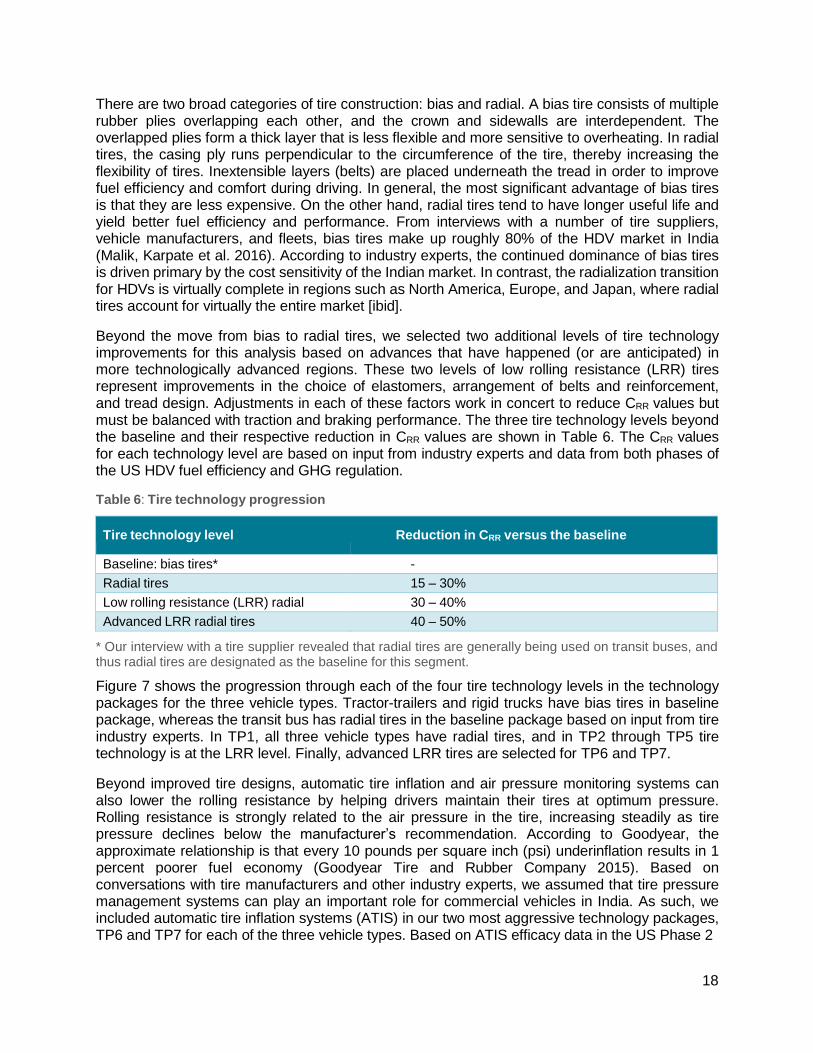
Beyond the move from bias to radial tires, we selected two additional levels of tire technology improvements for this analysis based on advances that have happened (or are anticipated) in more technologically advanced regions. These two levels of low rolling resistance (LRR) tires represent improvements in the choice of elastomers, arrangement of belts and reinforcement, and tread design. Adjustments in each of these factors work in concert to reduce CRR values but must be balanced with traction and braking performance. The three tire technology levels beyond the baseline and their respective reduction in CRR values are shown in Table 6. The CRR values for each technology level are based on input from industry experts and data from both phases of the US HDV fuel efficiency and GHG regulation.

Table 6: Tire technology progression

Tire technology level Reduction in CRR versus the baseline

Baseline: bias tires* -

Radial tires 15 – 30%

Low rolling resistance (LRR) radial 30 – 40%

Advanced LRR radial tires 40 – 50%

* Our interview with a tire supplier revealed that radial tires are generally being used on transit buses, and thus radial tires are designated as the baseline for this segment.

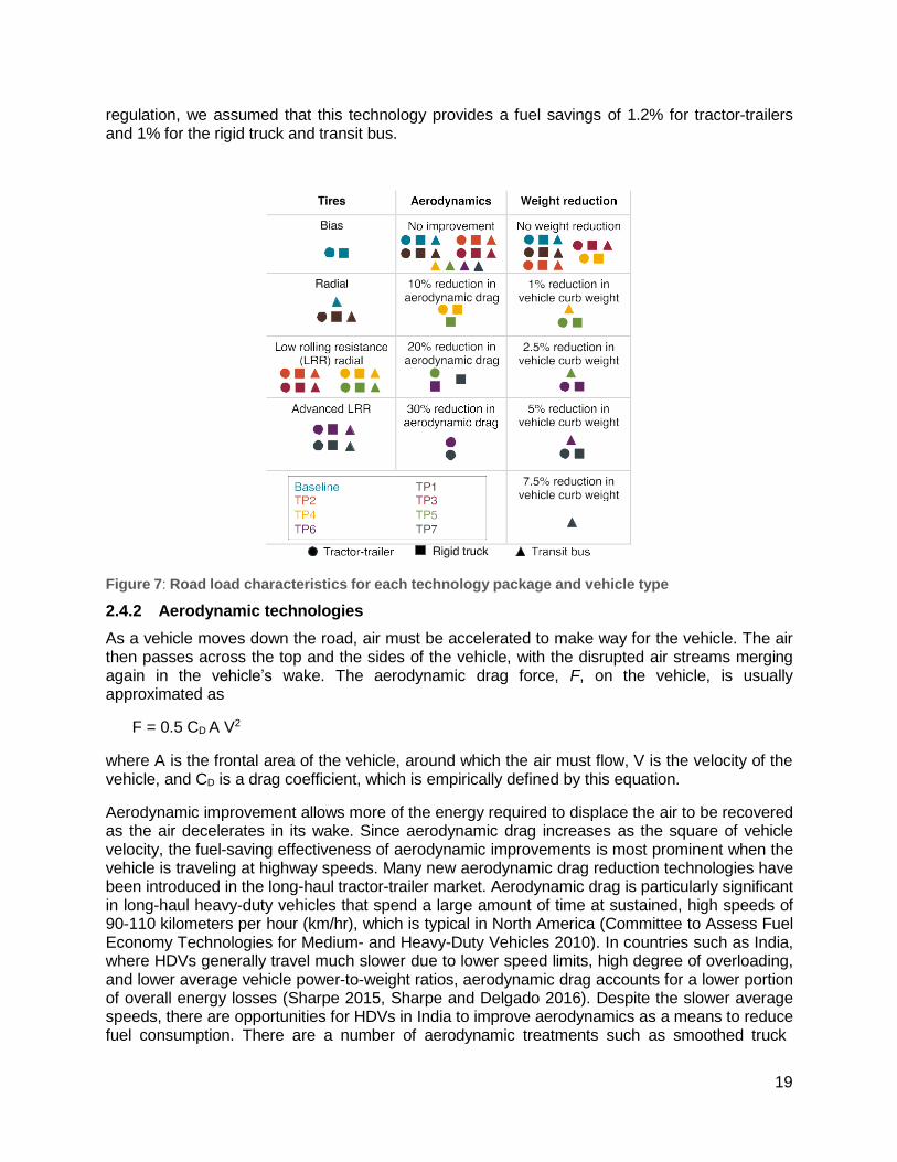
Figure 7 shows the progression through each of the four tire technology levels in the technology packages for the three vehicle types. Tractor-trailers and rigid trucks have bias tires in baseline package, whereas the transit bus has radial tires in the baseline package based on input from tire industry experts. In TP1, all three vehicle types have radial tires, and in TP2 through TP5 tire technology is at the LRR level. Finally, advanced LRR tires are selected for TP6 and TP7.

Beyond improved tire designs, automatic tire inflation and air pressure monitoring systems can also lower the rolling resistance by helping drivers maintain their tires at optimum pressure. Rolling resistance is strongly related to the air pressure in the tire, increasing steadily as tire pressure declines below the manufacturer’s recommendation. According to Goodyear, the approximate relationship is that every 10 pounds per square inch (psi) underinflation results in 1 percent poorer fuel economy (Goodyear Tire and Rubber Company 2015). Based on conversations with tire manufacturers and other industry experts, we assumed that tire pressure management systems can play an important role for commercial vehicles in India. As such, we included automatic tire inflation systems (ATIS) in our two most aggressive technology packages, TP6 and TP7 for each of the three vehicle types. Based on ATIS efficacy data in the US Phase 2

19

regulation, we assumed that this technology provides a fuel savings of 1.2% for tractor-trailers and 1% for the rigid truck and transit bus.

Figure 7: Road load characteristics for each technology package and vehicle type

2.4.2 Aerodynamic technologies

As a vehicle moves down the road, air must be accelerated to make way for the vehicle. The air then passes across the top and the sides of the vehicle, with the disrupted air streams merging again in the vehicle’s wake. The aerodynamic drag force, F, on the vehicle, is usually approximated as

F = 0.5 CD A V2

where A is the frontal area of the vehicle, around which the air must flow, V is the velocity of the vehicle, and CD is a drag coefficient, which is empirically defined by this equation.

Aerodynamic improvement allows more of the energy required to displace the air to be recovered as the air decelerates in its wake. Since aerodynamic drag increases as the square of vehicle velocity, the fuel-saving effectiveness of aerodynamic improvements is most prominent when the vehicle is traveling at highway speeds. Many new aerodynamic drag reduction technologies have been introduced in the long-haul tractor-trailer market. Aerodynamic drag is particularly significant in long-haul heavy-duty vehicles that spend a large amount of time at sustained, high speeds of 90-110 kilometers per hour (km/hr), which is typical in North America (Committee to Assess Fuel Economy Technologies for Medium- and Heavy-Duty Vehicles 2010). In countries such as India, where HDVs generally travel much slower due to lower speed limits, high degree of overloading, and lower average vehicle power-to-weight ratios, aerodynamic drag accounts for a lower portion of overall energy losses (Sharpe 2015, Sharpe and Delgado 2016). Despite the slower average speeds, there are opportunities for HDVs in India to improve aerodynamics as a means to reduce fuel consumption. There are a number of aerodynamic treatments such as smoothed truck

20

features; integrated tractor-trailer design; tractor-trailer gap reduction; and trailer side, rear, or underbody devices that offer potential to reduce aerodynamic drag.

Given that each of the three vehicle types are somewhat unique in terms of their configuration and opportunities for fuel savings from aerodynamic technologies, the level of technology progression for aerodynamic is defined in terms of percent reduction in CD rather than the application of particular sets of technologies. As shown in Figure 7, the four aerodynamic levels selected for this analysis are no improvement (i.e., the baseline), and 10%, 20%, and 30% reduction in CD, respectively.

With the efficacy of aerodynamic improvements being so intimately tied to vehicle speed, advancements in this technology area are assumed to be most applicable to tractor-trailers. When compared to rigid trucks and transit buses, tractor-trailers spend the largest percentage of their time operating at near-constant highway speeds. Figure 7 illustrates the progression through the three non-baseline aerodynamic levels for tractor-trailers: 10% CD reduction in TP4, 20% for TP5, and 30% for TP6 and TP7. Aerodynamic technologies are also applied to rigid trucks, though not as aggressively, since these vehicles are assumed to spend much more of their time in lower- speed urban driving (see Table 1). Rigid trucks are at the 10% CD reduction in TP4 and TP5 and then max out at the 20% level in the final two packages. For this analysis, we assume that transit buses spend all of their time in slow, stop-and-go driving and therefore would not reap any cost- effective benefits from aerodynamic improvements. As such, all of the packages for the transit bus are at the ‘no improvement’ level in terms of aerodynamics. This assumption regarding the inapplicability of aerodynamic improvements to transit buses is congruent with other studies (Committee to Assess Fuel Economy Technologies for Medium- and Heavy-Duty Vehicles 2010, US Environmental Protection Agency 2011, Committee on Assessment of Technologies and Approaches for Reducing the Fuel Consumption of Medium- and Heavy-Duty Vehicles - Phase Two 2014, US Environmental Protection Agency and Department of Transportation 2016).

2.4.3 Weight reduction technologies

From a fundamental physics perspective, decreasing the weight of a vehicle reduces the forces needed to accelerate or decelerate the vehicle as well as the forces needed to overcome rolling resistance, which, as described above, are approximately proportional to the load on the tires. Across all types of HDVs—but particularly for tractor-trailers— manufacturers have commercialized and continue to develop products that utilize alternative materials such as aluminum and composites that lower the curb weight of the vehicle.

In addition to reducing inertial and rolling resistance forces, the efficiency benefits of weight reduction are compounded if the end user is able to increase the payload as a direct result of decreasing the empty weight of the vehicle. This dual benefit is most common in freight trucks that ‘weigh-out,’ i.e., reach the maximum allowable weight limit.

As with aerodynamics, improvements in weight reduction are expressed as a percent reduction, rather than an application of specific technologies. The five levels in this technology area are no weight reduction (i.e., the baseline), and then 5%, 10%, 15%, and 20% reduction in curb weight, respectively. For tractor-trailers and rigid trucks, the technology packages are identical in terms of weight reduction, with TP5, TP6, and TP7 having 5%, 10%, and 15% curb weight reduction, respectively. The progression for the transit bus is more aggressive, starting with a 5% reduction in TP4 and then incrementally reaching a 20% reduction by TP7. The somewhat more ambitious weight reduction assumption for the transit bus compared to the two truck types is supported in the literature (Committee to Assess Fuel Economy Technologies for Medium- and Heavy-Duty

21

Vehicles 2010) and also aims to make up for the fact that aerodynamics improvements are not incorporated in the transit bus in this study.

2.5 Technology package fuel consumption reduction and costs

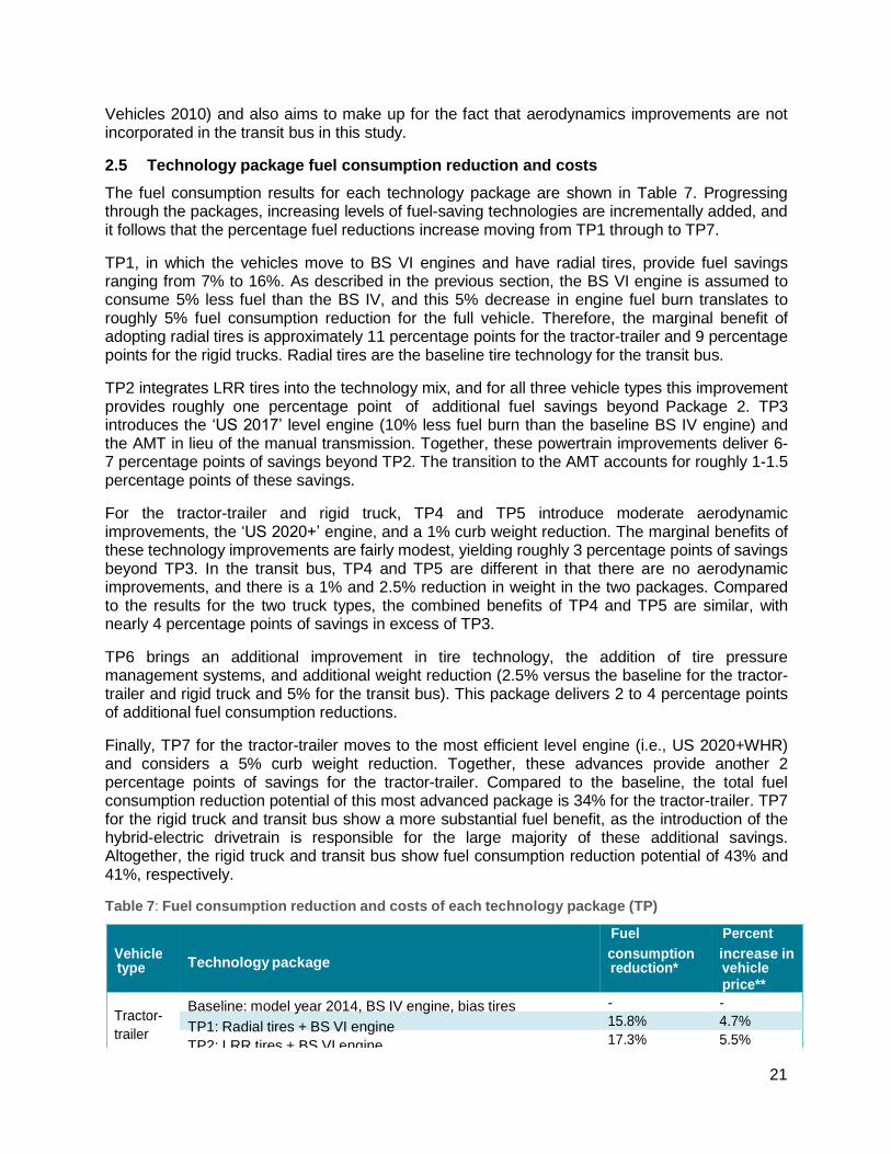
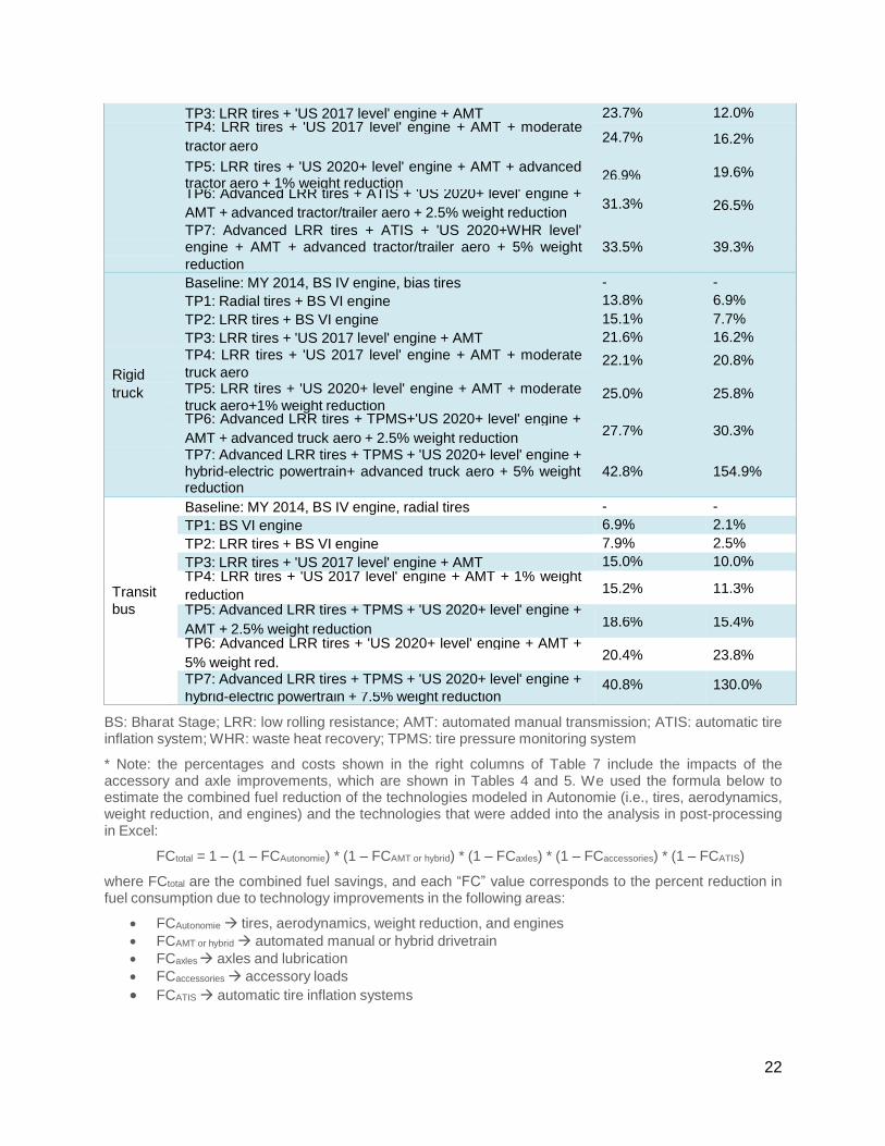
The fuel consumption results for each technology package are shown in Table 7. Progressing through the packages, increasing levels of fuel-saving technologies are incrementally added, and it follows that the percentage fuel reductions increase moving from TP1 through to TP7.

TP1, in which the vehicles move to BS VI engines and have radial tires, provide fuel savings ranging from 7% to 16%. As described in the previous section, the BS VI engine is assumed to consume 5% less fuel than the BS IV, and this 5% decrease in engine fuel burn translates to roughly 5% fuel consumption reduction for the full vehicle. Therefore, the marginal benefit of adopting radial tires is approximately 11 percentage points for the tractor-trailer and 9 percentage points for the rigid trucks. Radial tires are the baseline tire technology for the transit bus.

TP2 integrates LRR tires into the technology mix, and for all three vehicle types this improvement provides roughly one percentage point of additional fuel savings beyond Package 2. TP3 introduces the ‘US 2017’ level engine (10% less fuel burn than the baseline BS IV engine) and the AMT in lieu of the manual transmission. Together, these powertrain improvements deliver 6- 7 percentage points of savings beyond TP2. The transition to the AMT accounts for roughly 1-1.5 percentage points of these savings.

For the tractor-trailer and rigid truck, TP4 and TP5 introduce moderate aerodynamic improvements, the ‘US 2020+’ engine, and a 1% curb weight reduction. The marginal benefits of these technology improvements are fairly modest, yielding roughly 3 percentage points of savings beyond TP3. In the transit bus, TP4 and TP5 are different in that there are no aerodynamic improvements, and there is a 1% and 2.5% reduction in weight in the two packages. Compared to the results for the two truck types, the combined benefits of TP4 and TP5 are similar, with nearly 4 percentage points of savings in excess of TP3.

TP6 brings an additional improvement in tire technology, the addition of tire pressure management systems, and additional weight reduction (2.5% versus the baseline for the tractor- trailer and rigid truck and 5% for the transit bus). This package delivers 2 to 4 percentage points of additional fuel consumption reductions.

Finally, TP7 for the tractor-trailer moves to the most efficient level engine (i.e., US 2020+WHR) and considers a 5% curb weight reduction. Together, these advances provide another 2 percentage points of savings for the tractor-trailer. Compared to the baseline, the total fuel consumption reduction potential of this most advanced package is 34% for the tractor-trailer. TP7 for the rigid truck and transit bus show a more substantial fuel benefit, as the introduction of the hybrid-electric drivetrain is responsible for the large majority of these additional savings. Altogether, the rigid truck and transit bus show fuel consumption reduction potential of 43% and 41%, respectively.

Table 7: Fuel consumption reduction and costs of each technology package (TP)

Fuel Percent

Vehicle Technology package

consumption increase in type reduction* vehicle

price**

Tractor- Baseline: model year 2014, BS IV engine, bias tires

trailer TP1: Radial tires + BS VI engine

TP2: LRR tires + BS VI engine

-

15.8%

17.3%

-

4.7%

5.5%

22

TP3: LRR tires + 'US 2017 level' engine + AMT 23.7% 12.0% TP4: LRR tires + 'US 2017 level' engine + AMT + moderate

tractor aero 24.7%

16.2%

TP5: LRR tires + 'US 2020+ level' engine + AMT + advanced 26.9%

tractor aero + 1% weight reduction 19.6%

TP6: Advanced LRR tires + ATIS + 'US 2020+ level' engine +

AMT + advanced tractor/trailer aero + 2.5% weight reduction 31.3%

26.5%

TP7: Advanced LRR tires + ATIS + 'US 2020+WHR level' engine + AMT + advanced tractor/trailer aero + 5% weight 33.5% 39.3% reduction

Baseline: MY 2014, BS IV engine, bias tires - -

TP1: Radial tires + BS VI engine 13.8% 6.9%

TP2: LRR tires + BS VI engine 15.1% 7.7%

TP3: LRR tires + 'US 2017 level' engine + AMT 21.6% 16.2%

TP4: LRR tires + 'US 2017 level' engine + AMT + moderate 22.1% 20.8% Rigid truck aero truck TP5: LRR tires + 'US 2020+ level' engine + AMT + moderate 25.0% 25.8%

truck aero+1% weight reduction TP6: Advanced LRR tires + TPMS+'US 2020+ level' engine + AMT + advanced truck aero + 2.5% weight reduction 27.7% 30.3%

TP7: Advanced LRR tires + TPMS + 'US 2020+ level' engine + hybrid-electric powertrain+ advanced truck aero + 5% weight 42.8% 154.9% reduction Baseline: MY 2014, BS IV engine, radial tires - -

TP1: BS VI engine 6.9% 2.1%

TP2: LRR tires + BS VI engine 7.9% 2.5%

TP3: LRR tires + 'US 2017 level' engine + AMT 15.0% 10.0%

TP4: LRR tires + 'US 2017 level' engine + AMT + 1% weight Transit reduction 15.2% 11.3%

bus TP5: Advanced LRR tires + TPMS + 'US 2020+ level' engine + AMT + 2.5% weight reduction 18.6% 15.4%

TP6: Advanced LRR tires + 'US 2020+ level' engine + AMT + 5% weight red. 20.4% 23.8%

TP7: Advanced LRR tires + TPMS + 'US 2020+ level' engine + 40.8% 130.0% hybrid-electric powertrain + 7.5% weight reduction BS: Bharat Stage; LRR: low rolling resistance; AMT: automated manual transmission; ATIS: automatic tire inflation system; WHR: waste heat recovery; TPMS: tire pressure monitoring system

* Note: the percentages and costs shown in the right columns of Table 7 include the impacts of the accessory and axle improvements, which are shown in Tables 4 and 5. We used the formula below to estimate the combined fuel reduction of the technologies modeled in Autonomie (i.e., tires, aerodynamics, weight reduction, and engines) and the technologies that were added into the analysis in post-processing in Excel:

FCtotal = 1 – (1 – FCAutonomie) * (1 – FCAMT or hybrid) * (1 – FCaxles) * (1 – FCaccessories) * (1 – FCATIS)

where FCtotal are the combined fuel savings, and each “FC” value corresponds to the percent reduction in fuel consumption due to technology improvements in the following areas:

FCAutonomie tires, aerodynamics, weight reduction, and engines

FCAMT or hybrid automated manual or hybrid drivetrain FCaxles axles and lubrication

FCaccessories accessory loads

FCATIS automatic tire inflation systems

23

** Costs represent full costs to the end user and include taxes (12.5% for trucks and 30% per buses) and a 20% markup.

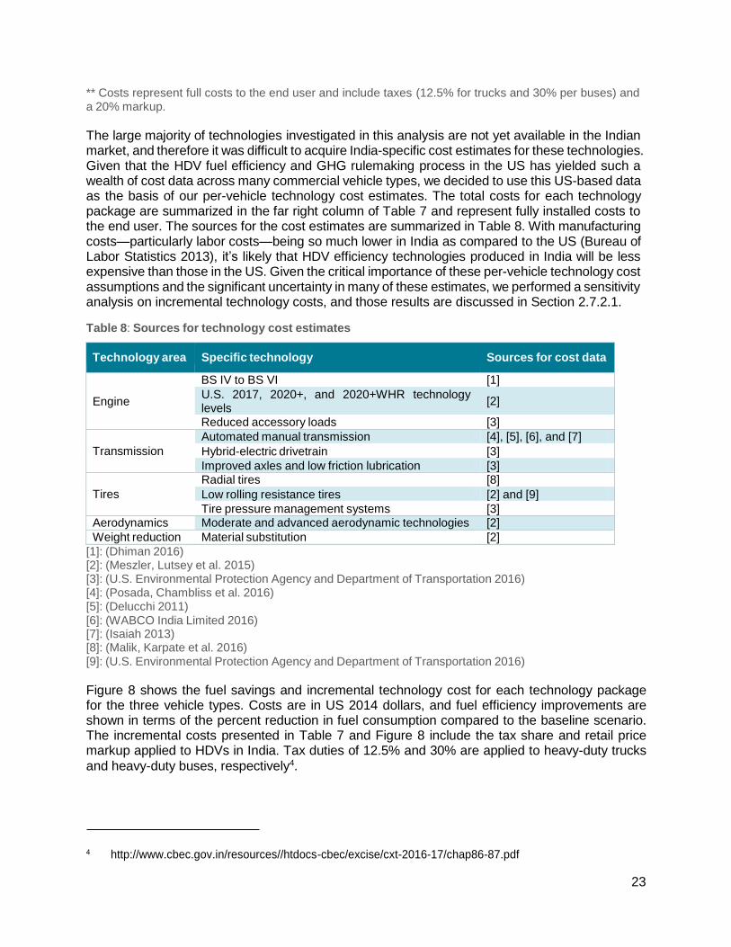
The large majority of technologies investigated in this analysis are not yet available in the Indian market, and therefore it was difficult to acquire India-specific cost estimates for these technologies. Given that the HDV fuel efficiency and GHG rulemaking process in the US has yielded such a wealth of cost data across many commercial vehicle types, we decided to use this US-based data as the basis of our per-vehicle technology cost estimates. The total costs for each technology package are summarized in the far right column of Table 7 and represent fully installed costs to the end user. The sources for the cost estimates are summarized in Table 8. With manufacturing costs—particularly labor costs—being so much lower in India as compared to the US (Bureau of Labor Statistics 2013), it’s likely that HDV efficiency technologies produced in India will be less expensive than those in the US. Given the critical importance of these per-vehicle technology cost assumptions and the significant uncertainty in many of these estimates, we performed a sensitivity analysis on incremental technology costs, and those results are discussed in Section 2.7.2.1.

Table 8: Sources for technology cost estimates

Technology area Specific technology Sources for cost data

BS IV to BS VI [1]

Engine U.S. 2017, 2020+, and 2020+WHR technology levels

[2]

Reduced accessory loads [3] Transmission

Automated manual transmission [4], [5], [6], and [7] Hybrid-electric drivetrain [3] Improved axles and low friction lubrication [3]

Tires

Radial tires [8] Low rolling resistance tires [2] and [9] Tire pressure management systems [3]

Aerodynamics Moderate and advanced aerodynamic technologies [2] Weight reduction Material substitution [2]

[1]: (Dhiman 2016) [2]: (Meszler, Lutsey et al. 2015) [3]: (U.S. Environmental Protection Agency and Department of Transportation 2016) [4]: (Posada, Chambliss et al. 2016) [5]: (Delucchi 2011) [6]: (WABCO India Limited 2016) [7]: (Isaiah 2013) [8]: (Malik, Karpate et al. 2016) [9]: (U.S. Environmental Protection Agency and Department of Transportation 2016)

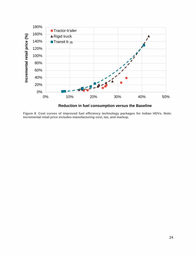
Figure 8 shows the fuel savings and incremental technology cost for each technology package for the three vehicle types. Costs are in US 2014 dollars, and fuel efficiency improvements are shown in terms of the percent reduction in fuel consumption compared to the baseline scenario. The incremental costs presented in Table 7 and Figure 8 include the tax share and retail price markup applied to HDVs in India. Tax duties of 12.5% and 30% are applied to heavy-duty trucks

and heavy-duty buses, respectively4.

4 http://www.cbec.gov.in/resources//htdocs-cbec/excise/cxt-2016-17/chap86-87.pdf

http://www.cbec.gov.in/resources/htdocs-cbec/excise/cxt-2016-17/chap86-87.pdf

24

180%

160%

140%

120%

100%

80%

60%

40%

20%

0%

0% 10% 20% 30% 40% 50%

Reduction in fuel consumption versus the Baseline

Figure 8: Cost curves of improved fuel efficiency technology packages for Indian HDVs. Note: Incremental retail price includes manufacturing cost, tax, and markup.

Tractor-tr ailer

k

us

Rigid truc

Transit b

Inc

rem

en

tal re

tail p

ric

e (

%)

25

2.6 Benefit cost analysis methodology and key assumptions

Benefit cost analysis (BCA) is calculated by summing the costs and benefits of each technology package over the lifetime of the vehicle and converted into a net present value (NPV) using a discount rate. The payback period (in years) for each technology package is calculated using the annual fuel savings provided by that technology package relative to the baseline.

The overall structure of the HDV BCA model is shown in Figure 9, which displays the benefits included: (1) Fuel cost savings, (2) Economic value of reduced greenhouse gas emissions and air pollution, (3) Reduction in refueling time, and (4) Improvements in energy security due to oil import reductions. The analysis includes the following parameters: annual vehicle kilometers traveled (VKT), vehicle fuel efficiency, vehicle lifetimes, fuel prices, driver labor rates, vehicle taxes, discount and interest rates, and incremental technology costs.

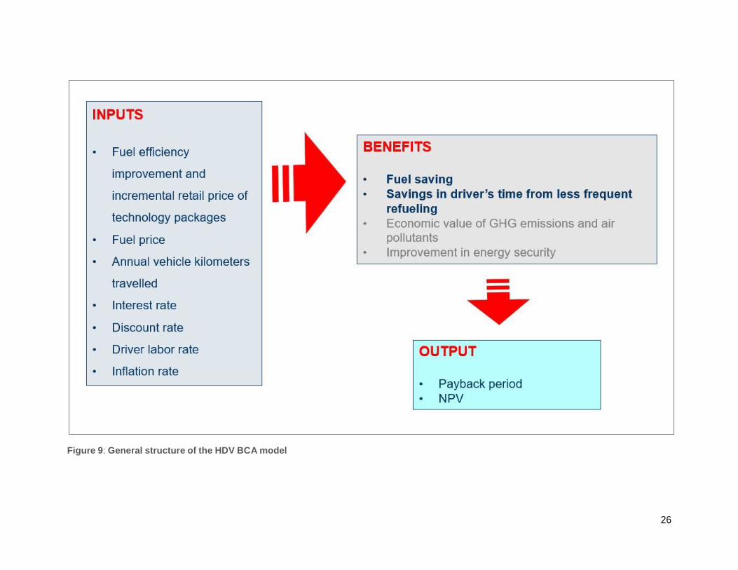
Figure 9: General structure of the HDV BCA model

26

27

Assumed values for the parameters used in this study are defined in detail later in this section. The impacts of varying the most significant parameters are assessed in the sensitivity analysis. Upon analyzing benefit cost results, attention is paid to the NPV of technology packages. NPV is used to identify the technology packages that create net positive economic value for the end user over the lifetime of the vehicle. The four benefits listed in the previous paragraph (and shown in Figure 9) are calculated as the change between the baseline scenario and the TP scenario, e.g., comparing the total cost of fuel in the baseline scenario and the TP scenario:

� � � � � � � (� )1≤� ≤5, = � � � � � � � � � (� )� 𝑎� � � 𝑖� � − � � � � � � � � � (� )𝑇𝑃 (Eq.1)

𝑁𝑃𝑉 = ∑�

𝑁 � � � � � � � 𝑖�

� =1 (1+� 𝑖� � � � � � )𝑡−1

(Eq.2)

where discount is the discount rate x represents the five benefits included in BCA framework t is the time in years

Total costs are subtracted from total benefits to calculate net benefit. Refer to Appendix A for mathematical modeling of variables, costs, and benefits.

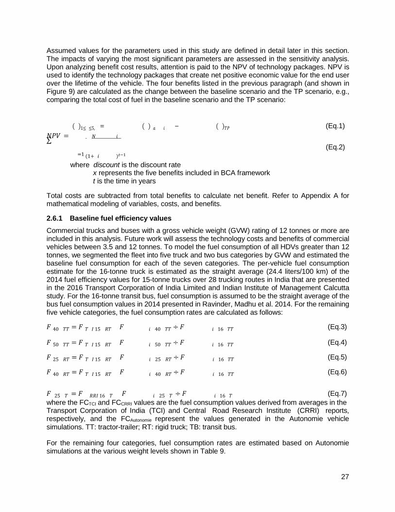
2.6.1 Baseline fuel efficiency values

Commercial trucks and buses with a gross vehicle weight (GVW) rating of 12 tonnes or more are included in this analysis. Future work will assess the technology costs and benefits of commercial vehicles between 3.5 and 12 tonnes. To model the fuel consumption of all HDVs greater than 12 tonnes, we segmented the fleet into five truck and two bus categories by GVW and estimated the baseline fuel consumption for each of the seven categories. The per-vehicle fuel consumption estimate for the 16-tonne truck is estimated as the straight average (24.4 liters/100 km) of the 2014 fuel efficiency values for 15-tonne trucks over 28 trucking routes in India that are presented in the 2016 Transport Corporation of India Limited and Indian Institute of Management Calcutta study. For the 16-tonne transit bus, fuel consumption is assumed to be the straight average of the bus fuel consumption values in 2014 presented in Ravinder, Madhu et al. 2014. For the remaining five vehicle categories, the fuel consumption rates are calculated as follows:

𝐹 40� 𝑇𝑇 = 𝐹 𝑇� 𝐼 15� 𝑅𝑇 � 𝐹 � � � � � � � 𝑖� 40� 𝑇𝑇 ÷ 𝐹 � � � � � � � 𝑖� 16� 𝑇𝑇 (Eq.3)

𝐹 50� 𝑇𝑇 = 𝐹 𝑇� 𝐼 15� 𝑅𝑇 � 𝐹 � � � � � � � 𝑖� 50� 𝑇𝑇 ÷ 𝐹 � � � � � � � 𝑖� 16� 𝑇𝑇 (Eq.4)

𝐹 25� 𝑅𝑇 = 𝐹 𝑇� 𝐼 15� 𝑅𝑇 � 𝐹 � � � � � � � 𝑖� 25� 𝑅𝑇 ÷ 𝐹 � � � � � � � 𝑖� 16� 𝑇𝑇 (Eq.5)

𝐹 40� 𝑅𝑇 = 𝐹 𝑇� 𝐼 15� 𝑅𝑇 � 𝐹 � � � � � � � 𝑖� 40� 𝑅𝑇 ÷ 𝐹 � � � � � � � 𝑖� 16� 𝑇𝑇 (Eq.6)

𝐹 25� 𝑇 = 𝐹 � 𝑅𝑅𝐼 16� 𝑇 � 𝐹 � � � � � � � 𝑖� 25� 𝑇 ÷ 𝐹 � � � � � � � 𝑖� 16� 𝑇 (Eq.7) where the FCTCI and FCCRRI values are the fuel consumption values derived from averages in the Transport Corporation of India (TCI) and Central Road Research Institute (CRRI) reports, respectively, and the FCAutonomie represent the values generated in the Autonomie vehicle simulations. TT: tractor-trailer; RT: rigid truck; TB: transit bus.

For the remaining four categories, fuel consumption rates are estimated based on Autonomie simulations at the various weight levels shown in Table 9.

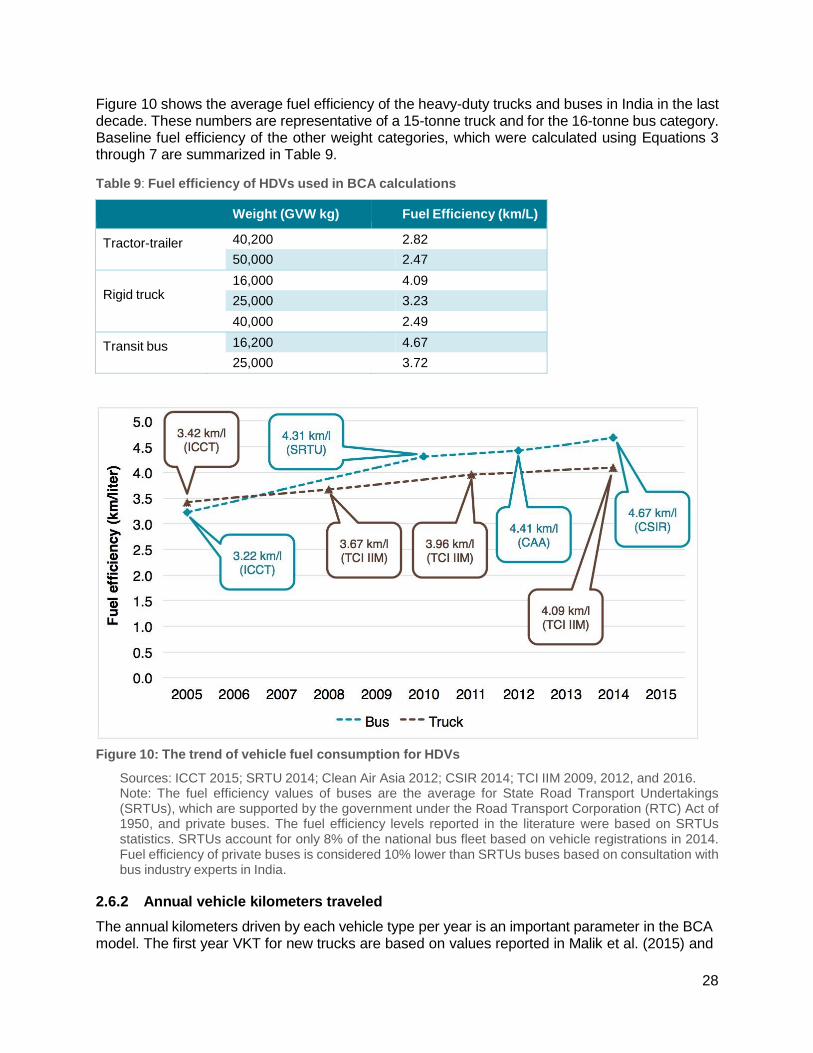
28

Figure 10 shows the average fuel efficiency of the heavy-duty trucks and buses in India in the last decade. These numbers are representative of a 15-tonne truck and for the 16-tonne bus category. Baseline fuel efficiency of the other weight categories, which were calculated using Equations 3 through 7 are summarized in Table 9.

Table 9: Fuel efficiency of HDVs used in BCA calculations

Weight (GVW kg) Fuel Efficiency (km/L)

Tractor-trailer 40,200 2.82

50,000 2.47

16,000 4.09 Rigid truck

25,000 3.23

40,000 2.49

Transit bus 16,200 4.67

25,000 3.72

Figure 10: The trend of vehicle fuel consumption for HDVs

Sources: ICCT 2015; SRTU 2014; Clean Air Asia 2012; CSIR 2014; TCI IIM 2009, 2012, and 2016. Note: The fuel efficiency values of buses are the average for State Road Transport Undertakings (SRTUs), which are supported by the government under the Road Transport Corporation (RTC) Act of 1950, and private buses. The fuel efficiency levels reported in the literature were based on SRTUs statistics. SRTUs account for only 8% of the national bus fleet based on vehicle registrations in 2014. Fuel efficiency of private buses is considered 10% lower than SRTUs buses based on consultation with bus industry experts in India.

2.6.2 Annual vehicle kilometers traveled

The annual kilometers driven by each vehicle type per year is an important parameter in the BCA model. The first year VKT for new trucks are based on values reported in Malik et al. (2015) and

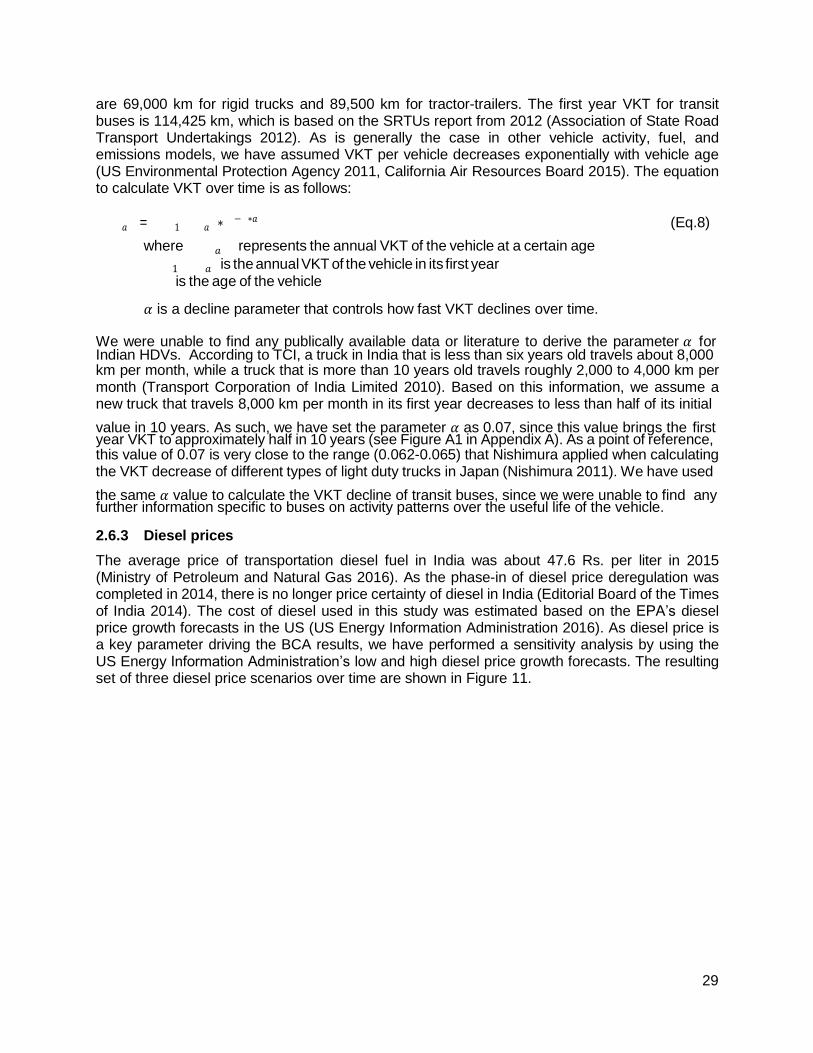
29

are 69,000 km for rigid trucks and 89,500 km for tractor-trailers. The first year VKT for transit buses is 114,425 km, which is based on the SRTUs report from 2012 (Association of State Road Transport Undertakings 2012). As is generally the case in other vehicle activity, fuel, and emissions models, we have assumed VKT per vehicle decreases exponentially with vehicle age (US Environmental Protection Agency 2011, California Air Resources Board 2015). The equation to calculate VKT over time is as follows:

� � � 𝑎� � = � � � 1� � � � 𝑎� ∗ � −� ∗𝑎� � (Eq.8)

where � � � 𝑎� � represents the annual VKT of the vehicle at a certain age

� � � 1� � � � 𝑎� is the annual VKT of the vehicle in its first year

� � � is the age of the vehicle

𝛼 is a decline parameter that controls how fast VKT declines over time.

We were unable to find any publically available data or literature to derive the parameter 𝛼 for Indian HDVs. According to TCI, a truck in India that is less than six years old travels about 8,000 km per month, while a truck that is more than 10 years old travels roughly 2,000 to 4,000 km per month (Transport Corporation of India Limited 2010). Based on this information, we assume a new truck that travels 8,000 km per month in its first year decreases to less than half of its initial

value in 10 years. As such, we have set the parameter 𝛼 as 0.07, since this value brings the first year VKT to approximately half in 10 years (see Figure A1 in Appendix A). As a point of reference, this value of 0.07 is very close to the range (0.062-0.065) that Nishimura applied when calculating the VKT decrease of different types of light duty trucks in Japan (Nishimura 2011). We have used

the same 𝛼 value to calculate the VKT decline of transit buses, since we were unable to find any further information specific to buses on activity patterns over the useful life of the vehicle.

2.6.3 Diesel prices

The average price of transportation diesel fuel in India was about 47.6 Rs. per liter in 2015 (Ministry of Petroleum and Natural Gas 2016). As the phase-in of diesel price deregulation was completed in 2014, there is no longer price certainty of diesel in India (Editorial Board of the Times of India 2014). The cost of diesel used in this study was estimated based on the EPA’s diesel price growth forecasts in the US (US Energy Information Administration 2016). As diesel price is a key parameter driving the BCA results, we have performed a sensitivity analysis by using the US Energy Information Administration’s low and high diesel price growth forecasts. The resulting set of three diesel price scenarios over time are shown in Figure 11.

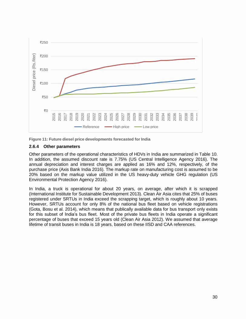
30

₹250

₹200

₹150

₹100

₹50

₹0

Reference High price Low price

Figure 11: Future diesel price developments forecasted for India

2.6.4 Other parameters

Other parameters of the operational characteristics of HDVs in India are summarized in Table 10. In addition, the assumed discount rate is 7.75% (US Central Intelligence Agency 2016). The annual depreciation and interest charges are applied as 16% and 12%, respectively, of the purchase price (Axis Bank India 2016). The markup rate on manufacturing cost is assumed to be 20% based on the markup value utilized in the US heavy-duty vehicle GHG regulation (US Environmental Protection Agency 2016).

In India, a truck is operational for about 20 years, on average, after which it is scrapped (International Institute for Sustainable Development 2013). Clean Air Asia cites that 25% of buses registered under SRTUs in India exceed the scrapping target, which is roughly about 10 years. However, SRTUs account for only 8% of the national bus fleet based on vehicle registrations (Gota, Bosu et al. 2014), which means that publically available data for bus transport only exists for this subset of India’s bus fleet. Most of the private bus fleets in India operate a significant percentage of buses that exceed 15 years old (Clean Air Asia 2012). We assumed that average lifetime of transit buses in India is 18 years, based on these IISD and CAA references.

Die

se

l p

rice (

Rs./

lite

r)

2015

2016

2017

2018

2019

2020

2021

2022

2023

2024

2025

2026

2027

2028

2029

2030

2031

2032

2033

2034

2035

2036

2037

2038

2039

2040

31

Table 10: Operational characteristics of HDVs in India

Average lifetime (years)

Driver labor rate* Rs/hour)

Tank volume** (liters)

Fuel dispensing rate*** (liter/min)

Refueling fixed time*** (min/refill)

Tractor-trailer 20 ₹63 400 76 3.5

Rigid truck 20 ₹63 350 38 3.5

Transit bus 18 ₹63 250 38 3.5

* Source: TCI, 2016. The driver labor rate was increased by the inflation rate of 5.4% (Ministry of Statistics and Programme Implementation 2016) ** Source: Assumption based on vehicle specification sheets (Tata Motors 2016, Tata Motors 2016, Tata Motors 2016) *** Source: Assumption based on refueling rates presented in (US Environmental Protection Agency and Department of Transportation 2016)

Please note that we have not included any GHG damage costs or monetary benefits from increasing energy security in determining the technology package benefits in this analysis. This analysis purely focuses on the costs and benefits imposed on truck and bus owners and operators in India. However, the BCA model is capable of including these benefits in the BCA calculation. In this case, a careful analysis would be required to determine monetary value of GHGs and energy security increase in India. In addition, the model can also capture benefits of increased

vehicle use due to rebound effect5. Based on expert judgements, this analysis assumes that there would be no rebound effect in India due to lower fuel consumption. However, we evaluate the sensitivity of results to the rebound effect (see Section 2.7.2). The benefits that we include in our analysis are 1) fuel cost savings and 2) reduction in refueling time. The results are presented in the following section.

2.7 BCA results

2.7.1 BCA fuel efficiency scenario results

Seven different technology packages, summarized earlier in Table 7, were analyzed as fuel efficiency scenarios. We assumed that the packages can be deployed on new trucks and buses starting in 2020.

The overview of payback periods of the technology packages compared to the baseline scenario are illustrated in Figure 12 for the three primary weight categories that we analyzed in this project. Please see Appendix A for the results of the four other weight categories. The payback period for tractor-trailers is less than or equal to 1 year in the first six technology packages, i.e., TP1 to TP6, and the remaining package, i.e., TP7, repays the initial investment within 2 years. The payback periods for rigid trucks are less than or equal to 1 year in TP1, TP2, TP3, and TP4, and 2 years in the remaining packages. The exception is TP7 (payback time of 12 years), which adds the hybrid-electric system that is considerably more expensive than the other technologies included in the analysis. For transit buses, the first five packages payback within the first year of ownership; TP6 in 2 years; and TP7 in 12 years, respectively. The payback period and NPV (see Figures 12 and 13) are calculated assuming the vehicle is purchased with an initial one-time upfront payment.

5 Economic theory suggests that the resulting lower fuel consumption rates will lower the cost of driving and thus increase vehicle km traveled. The resulting increase in trucking km traveled is commonly referred to as the rebound

effect.

32

If we assume that the hybrid bus avails of the FAME incentive currently on offer, the payback period drops to zero (shown by the last bar in figure 12).

To finance vehicle acquisition, truck operators in India typically take a loan for 3 to 5 years (International Institute for Sustainable Development 2013). Once the loan has been repaid, truck operators tend to use the truck for two to three more years and then sell it in the second-hand truck market. Thus, in this study, we assume that the technology packages with a payback period of 3 years or less are cost competitive for the trucking industry, as well as the bus industry since we don’t have any further information for buses. We also performed a sensitivity analysis assuming a 5-year loan (see Figures 14 and 15). As expected, vehicle acquisition with a 5-year loan shortens the payback periods while decreasing the NPV results. However, results indicate that the decrease in NPV is fairly small for TP1 through TP6—between 0.3 and 1.8 lakhs. Total NPV of HDV fleet is also calculated by using the stock and sales forecasts discussed in the following section.

14 45%

12 40%

35%

10 30%

8 25%

6 20%

15% 4

10%

2 5%

0 0%

TP1 TP2 TP3 TP4 TP5 TP6 TP7


Figure 12: Payback periods for each technology package and vehicle type, assuming one-time upfront payment

Note: Bars represent payback and markers represent fuel consumption reduction. HDV categories illustrated here represents a 40-tonne tractor-trailer, 25-tonne rigid truck, and 16-tonne transit bus. See Appendix A for the other weight categories.

Fu

el co

nsu

mp

tio

n r

ed

ucti

on

(%

)

Payb

ack

(y

ears

)

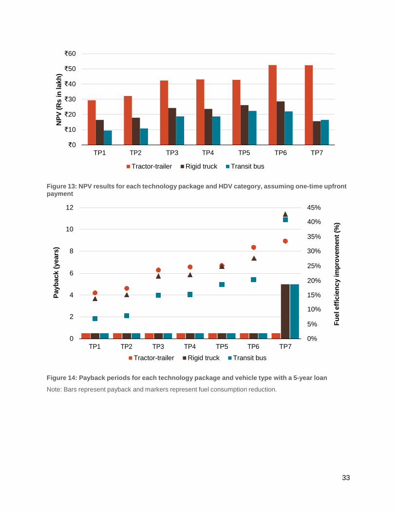
33

₹60

₹50

₹40

₹30

₹20

₹10

₹0 TP1 TP2 TP3 TP4 TP5 TP6 TP7


Figure 13: NPV results for each technology package and HDV category, assuming one-time upfront payment

12 45%

40% 10

35%

8 30%

25% 6

20%

4 15%

10% 2

5%

0 0% TP1 TP2 TP3 TP4 TP5 TP6 TP7


Figure 14: Payback periods for each technology package and vehicle type with a 5-year loan

Note: Bars represent payback and markers represent fuel consumption reduction.

NP

V (

Rs

in

lakh

)

Fu

el e

ffic

ien

cy

im

pro

vem

en

t (%

)

Payb

ack

(y

ears

)

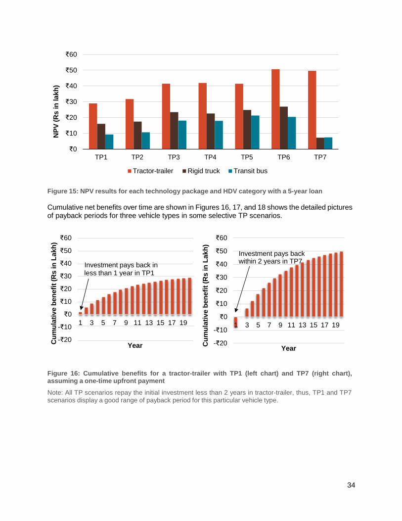
34

Cu

mu

lati

ve

ben

efi

t (R

s in

La

kh

)

Investment pays back within 2 years in TP7

1 3 5 7 9 11 13 15 17 19

₹60

₹50

₹40

₹30

₹20

₹10

₹0 TP1 TP2 TP3 TP4 TP5 TP6 TP7


Figure 15: NPV results for each technology package and HDV category with a 5-year loan

Cumulative net benefits over time are shown in Figures 16, 17, and 18 shows the detailed pictures of payback periods for three vehicle types in some selective TP scenarios.

₹60

₹50

₹40

₹30

₹20

₹10

₹0

-₹10

-₹20

Investment pays back in

less than 1 year in TP1

1 3 5 7 9 11 13 15 17 19

Year

₹60

₹50

₹40

₹30

₹20

₹10

₹0

-₹10

-₹20

Year

Figure 16: Cumulative benefits for a tractor-trailer with TP1 (left chart) and TP7 (right chart), assuming a one-time upfront payment

Note: All TP scenarios repay the initial investment less than 2 years in tractor-trailer, thus, TP1 and TP7 scenarios display a good range of payback period for this particular vehicle type.

NP

V (

Rs

in

la

kh

)

Cu

mu

lati

ve

ben

efi

t (R

s in

La

kh

)

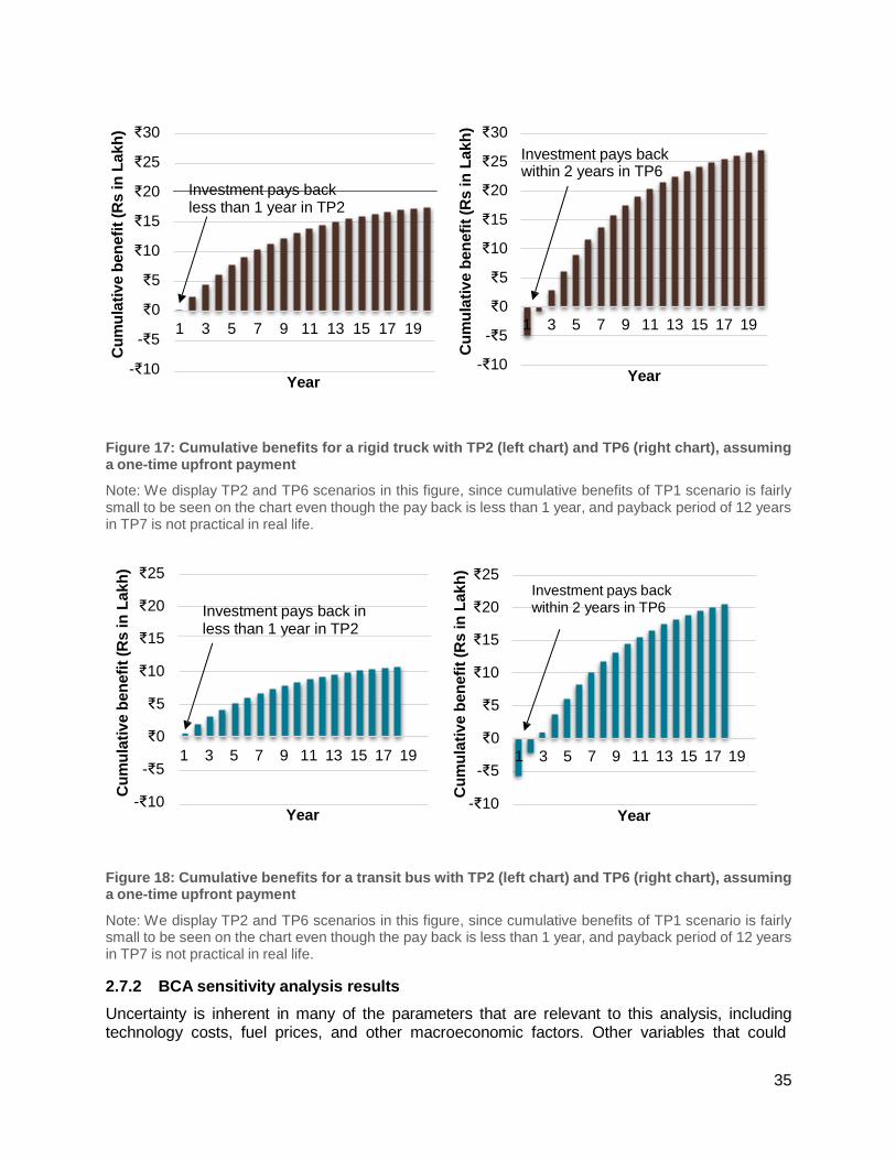
35


1 3 5 7 9 11 13 15 17 19

Cu

mu

lati

ve

ben

efi

t (R

s in

La

kh

)

₹30

₹25

₹20

₹15

₹10

₹5

₹0

-₹5

-₹10

Investment pays back less than 1 year in TP2

1 3 5 7 9 11 13 15 17 19

Year

₹30

₹25

₹20

₹15

₹10

₹5

₹0

-₹5

-₹10

Year

Figure 17: Cumulative benefits for a rigid truck with TP2 (left chart) and TP6 (right chart), assuming a one-time upfront payment

Note: We display TP2 and TP6 scenarios in this figure, since cumulative benefits of TP1 scenario is fairly small to be seen on the chart even though the pay back is less than 1 year, and payback period of 12 years in TP7 is not practical in real life.

₹25

₹20

₹15

₹10

₹5

₹0

-₹5

-₹10

Investment pays back in less than 1 year in TP2

1 3 5 7 9 11 13 15 17 19

Year

₹25

₹20

₹15

₹10

₹5

₹0

-₹5

-₹10


1 3 5 7 9 11 13 15 17 19

Year

Figure 18: Cumulative benefits for a transit bus with TP2 (left chart) and TP6 (right chart), assuming a one-time upfront payment

Note: We display TP2 and TP6 scenarios in this figure, since cumulative benefits of TP1 scenario is fairly small to be seen on the chart even though the pay back is less than 1 year, and payback period of 12 years in TP7 is not practical in real life.

2.7.2 BCA sensitivity analysis results

Uncertainty is inherent in many of the parameters that are relevant to this analysis, including technology costs, fuel prices, and other macroeconomic factors. Other variables that could

Cu

mu

lati

ve

ben

efi

t (R

s in

La

kh

)

Cu

mu

lati

ve

ben

efi

t (R

s in

La

kh

)

Cu

mu

lati

ve

ben

efi

t (R

s in

La

kh

)

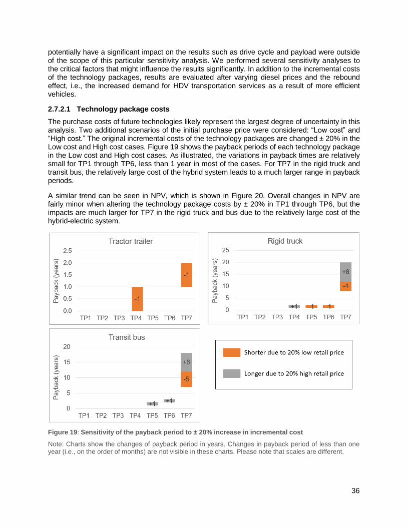
36

potentially have a significant impact on the results such as drive cycle and payload were outside of the scope of this particular sensitivity analysis. We performed several sensitivity analyses to the critical factors that might influence the results significantly. In addition to the incremental costs of the technology packages, results are evaluated after varying diesel prices and the rebound effect, i.e., the increased demand for HDV transportation services as a result of more efficient vehicles.

2.7.2.1 Technology package costs

The purchase costs of future technologies likely represent the largest degree of uncertainty in this analysis. Two additional scenarios of the initial purchase price were considered: “Low cost” and “High cost.” The original incremental costs of the technology packages are changed ± 20% in the Low cost and High cost cases. Figure 19 shows the payback periods of each technology package in the Low cost and High cost cases. As illustrated, the variations in payback times are relatively small for TP1 through TP6, less than 1 year in most of the cases. For TP7 in the rigid truck and transit bus, the relatively large cost of the hybrid system leads to a much larger range in payback periods.

A similar trend can be seen in NPV, which is shown in Figure 20. Overall changes in NPV are fairly minor when altering the technology package costs by ± 20% in TP1 through TP6, but the impacts are much larger for TP7 in the rigid truck and bus due to the relatively large cost of the hybrid-electric system.

Figure 19: Sensitivity of the payback period to ± 20% increase in incremental cost

Note: Charts show the changes of payback period in years. Changes in payback period of less than one year (i.e., on the order of months) are not visible in these charts. Please note that scales are different.

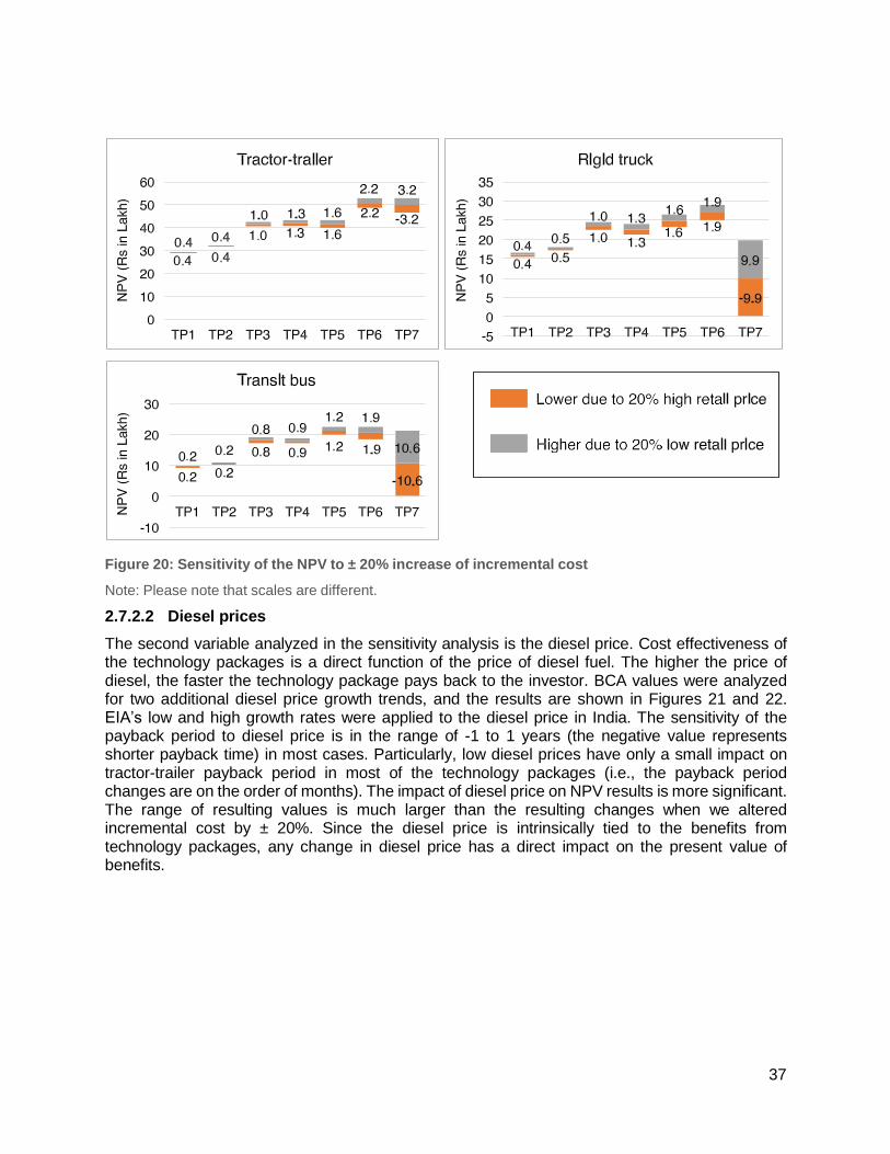
37

Figure 20: Sensitivity of the NPV to ± 20% increase of incremental cost

Note: Please note that scales are different.

2.7.2.2 Diesel prices

The second variable analyzed in the sensitivity analysis is the diesel price. Cost effectiveness of the technology packages is a direct function of the price of diesel fuel. The higher the price of diesel, the faster the technology package pays back to the investor. BCA values were analyzed for two additional diesel price growth trends, and the results are shown in Figures 21 and 22. EIA’s low and high growth rates were applied to the diesel price in India. The sensitivity of the payback period to diesel price is in the range of -1 to 1 years (the negative value represents shorter payback time) in most cases. Particularly, low diesel prices have only a small impact on tractor-trailer payback period in most of the technology packages (i.e., the payback period changes are on the order of months). The impact of diesel price on NPV results is more significant. The range of resulting values is much larger than the resulting changes when we altered incremental cost by ± 20%. Since the diesel price is intrinsically tied to the benefits from technology packages, any change in diesel price has a direct impact on the present value of benefits.

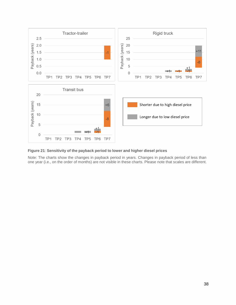
38

Figure 21: Sensitivity of the payback period to lower and higher diesel prices

Note: The charts show the changes in payback period in years. Changes in payback period of less than one year (i.e., on the order of months) are not visible in these charts. Please note that scales are different.

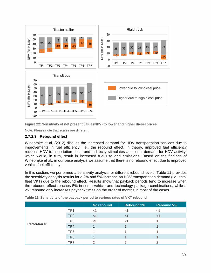
39

Tractor-trailer

Figure 22: Sensitivity of net present value (NPV) to lower and higher diesel prices

Note: Please note that scales are different.

2.7.2.3 Rebound effect

Winebrake et al. (2012) discuss the increased demand for HDV transportation services due to improvements in fuel efficiency, i.e., the rebound effect. In theory, improved fuel efficiency reduces HDV transportation costs and indirectly stimulates additional demand for HDV activity, which would, in turn, result in increased fuel use and emissions. Based on the findings of Winebrake et al., in our base analysis we assume that there is no rebound effect due to improved vehicle fuel efficiency.

In this section, we performed a sensitivity analysis for different rebound levels. Table 11 provides the sensitivity analysis results for a 2% and 5% increase on HDV transportation demand (i.e., total fleet VKT) due to the rebound effect. Results show that payback periods tend to increase when the rebound effect reaches 5% in some vehicle and technology package combinations, while a 2% rebound only increases payback times on the order of months in most of the cases.

Table 11: Sensitivity of the payback period to various rates of VKT rebound

No rebound Rebound 2% Rebound 5%

TP1 <1 <1 <1

TP2 <1 <1 <1

TP3 <1 <1 1

TP4 1 1 1

TP5 1 1 1

TP6 1 1 1

TP7 2 2 2

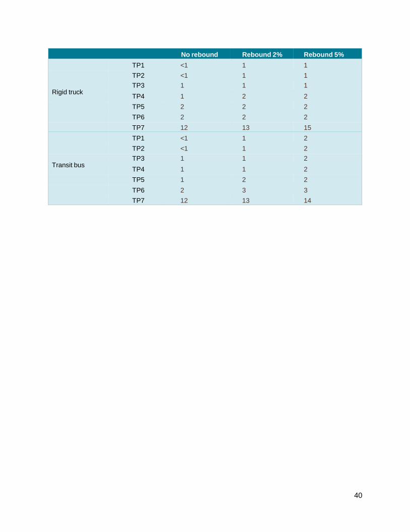
40

No rebound Rebound 2% Rebound 5%

TP1 <1 1 1

TP2 <1 1 1

TP3 1 1 1 Rigid truck

TP4 1 2 2

TP5 2 2 2

TP6 2 2 2

TP7 12 13 15

TP1 <1 1 2

TP2 <1 1 2

TP3 1 1 2 Transit bus

TP4 1 1 2

TP5 1 2 2

TP6 2 3 3

TP7 12 13 14

41

3 Oil and CO2 emissions projections

This section investigates the fuel savings and CO2 emissions reduction potential of the fuel efficiency improvements in the seven different HDV technology packages.

3.1 HDV energy model and key assumptions

The HDV fleet energy model estimates and projects annual vehicle sales and stock, annual total vehicle kilometers traveled, annual fuel consumption, average fleet efficiency, and GHG and air pollutant emissions of HDVs. The model includes the years 2000 to 2050 and has annual time- steps. The initial year of our fleet analysis is 2015, and the model is calibrated against the historical data between 2000 and 2014.

The model is built upon three modules; (1) a demand module, (2) a vehicle stock turnover module, and (3) an efficient technology module. The details of the modules are explained below. The overall structure of the HDV fleet model is given in Figure 23, which shows the input requirements and the flow of inputs and outputs.

Figure 23: HDV fleet energy model

42

43

The model begins by generating annual vehicle demand in the Demand Module based on annual demand growth and scrappage of existing HDVs greater than 12 tonnes GVW for three types of vehicles: tractor-trailers, rigid trucks, and transit buses. The annual demand growth rate for each vehicle type is defined based on a regression analysis where GDP growth was used as a dependent variable. The literature around scrappage rates of motor vehicles, particularly HDVs, is very limited. For this study, India-specific scrappage rates are calculated through logistic functions. Vehicle demand in the calibration period, i.e., 2000-2014, is based on stock statistics from the ICCT. The Stock Turnover Module determines the new vehicle fleet based on annual vehicle demand, scrappage of existing stock, and exogenous market penetration of technology packages, inputted from the Efficient Technology Module. The stock turnover module includes the annual stock of trucks and buses, VKTs by vehicle type and age, fuel consumption, and GHG emissions. The rate of decline in VKT by vehicle age, fleet utilization, fuel economy, and emission factors are key parameters that are considered in this module. The assumptions and formulas used in the model are explained in detail in the following sections and Appendix B.

3.1.1 Demand projection

Annual HDV demand (in number of vehicles in stock) in India was projected from the 2015 baseline to 2050 using regression analysis. The projections were disaggregated at the level of HDV type—i.e., tractor-trailer, rigid truck, and transit bus—and used as an input for the HDV stock turnover module.

HDV stock (in number of vehicles) increased at an average annual growth rate of 7.2%, between 2002 and 2012, while GDP grew at an average rate of 7.9%. The total length of roads increased at an average growth rate of 3.3% over this same period. Figure 24 shows the relationship between annual HDV stock and GDP in India between 2000 and 2014. As shown, the growth trends are very similar, which makes sense given that HDV activity—particularly that of freight trucks—is directly tied to economic productivity. In addition, Table 12 indicates that growth in HDV stock is significantly correlated with growth in GDP. Based on these findings, we have assumed that GDP is the key driver of annual HDV demand.

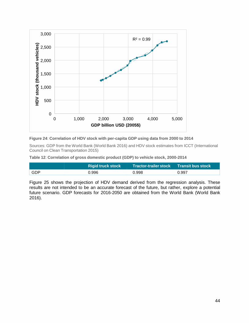
44

3,000

R² = 0.99

2,500

2,000

1,500

1,000

500

0 0 1,000 2,000 3,000 4,000 5,000

GDP billion USD (2005$)

Figure 24: Correlation of HDV stock with per-capita GDP using data from 2000 to 2014

Sources: GDP from the World Bank (World Bank 2016) and HDV stock estimates from ICCT (International Council on Clean Transportation 2015)

Table 12: Correlation of gross domestic product (GDP) to vehicle stock, 2000-2014

Rigid truck stock Tractor-trailer stock Transit bus stock

GDP 0.996 0.998 0.997

Figure 25 shows the projection of HDV demand derived from the regression analysis. These results are not intended to be an accurate forecast of the future, but rather, explore a potential future scenario. GDP forecasts for 2016-2050 are obtained from the World Bank (World Bank 2016).

HD

V s

toc

k (

tho

us

an

d v

eh

icle

s)

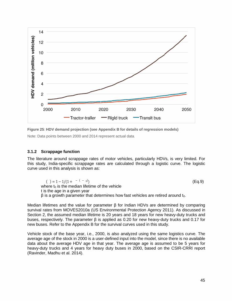
45

Figure 25: HDV demand projection (see Appendix B for details of regression models)

Note: Data points between 2000 and 2014 represent actual data.

3.1.2 Scrappage function

The literature around scrappage rates of motor vehicles, particularly HDVs, is very limited. For this study, India-specific scrappage rates are calculated through a logistic curve. The logistic curve used in this analysis is shown as:

� � � � � � � � (� ) = 1 − 1/(1 + � −� (� −� 0)) (Eq.9) where t0 is the median lifetime of the vehicle t is the age in a given year β is a growth parameter that determines how fast vehicles are retired around t0.

Median lifetimes and the value for parameter β for Indian HDVs are determined by comparing survival rates from MOVES2010a (US Environmental Protection Agency 2011). As discussed in Section 2, the assumed median lifetime is 20 years and 18 years for new heavy-duty trucks and buses, respectively. The parameter β is applied as 0.20 for new heavy-duty trucks and 0.17 for new buses. Refer to the Appendix B for the survival curves used in this study.

Vehicle stock of the base year, i.e., 2000, is also analyzed using the same logistics curve. The average age of the stock in 2000 is a user-defined input into the model, since there is no available data about the average HDV age in that year. The average age is assumed to be 5 years for heavy-duty trucks and 4 years for heavy duty buses in 2000, based on the CSIR-CRRI report (Ravinder, Madhu et al. 2014).

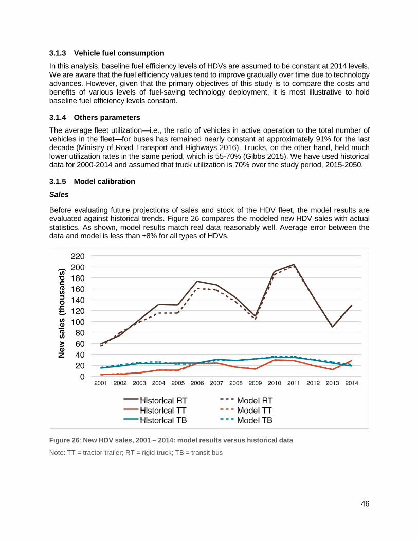
46

3.1.3 Vehicle fuel consumption

In this analysis, baseline fuel efficiency levels of HDVs are assumed to be constant at 2014 levels. We are aware that the fuel efficiency values tend to improve gradually over time due to technology advances. However, given that the primary objectives of this study is to compare the costs and benefits of various levels of fuel-saving technology deployment, it is most illustrative to hold baseline fuel efficiency levels constant.

3.1.4 Others parameters

The average fleet utilization—i.e., the ratio of vehicles in active operation to the total number of vehicles in the fleet—for buses has remained nearly constant at approximately 91% for the last decade (Ministry of Road Transport and Highways 2016). Trucks, on the other hand, held much lower utilization rates in the same period, which is 55-70% (Gibbs 2015). We have used historical data for 2000-2014 and assumed that truck utilization is 70% over the study period, 2015-2050.

3.1.5 Model calibration

Sales

Before evaluating future projections of sales and stock of the HDV fleet, the model results are evaluated against historical trends. Figure 26 compares the modeled new HDV sales with actual statistics. As shown, model results match real data reasonably well. Average error between the data and model is less than ±8% for all types of HDVs.

Figure 26: New HDV sales, 2001 – 2014: model results versus historical data

Note: TT = tractor-trailer; RT = rigid truck; TB = transit bus

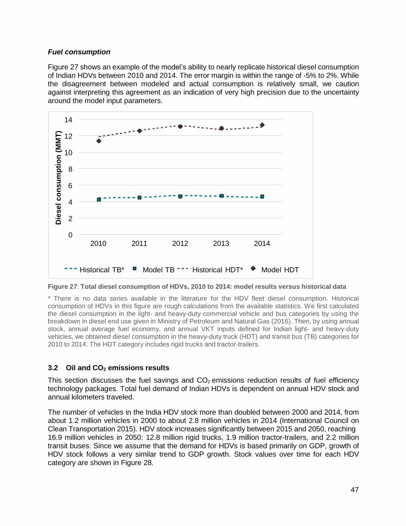
47

14

12

10

8

6

4

2

0 2010 2011 2012 2013 2014

Historical TB* Model TB Historical HDT* Model HDT

Fuel consumption

Figure 27 shows an example of the model’s ability to nearly replicate historical diesel consumption of Indian HDVs between 2010 and 2014. The error margin is within the range of -5% to 2%. While the disagreement between modeled and actual consumption is relatively small, we caution against interpreting this agreement as an indication of very high precision due to the uncertainty around the model input parameters.

Figure 27: Total diesel consumption of HDVs, 2010 to 2014: model results versus historical data

* There is no data series available in the literature for the HDV fleet diesel consumption. Historical consumption of HDVs in this figure are rough calculations from the available statistics. We first calculated the diesel consumption in the light- and heavy-duty commercial vehicle and bus categories by using the breakdown in diesel end use given in Ministry of Petroleum and Natural Gas (2016). Then, by using annual stock, annual average fuel economy, and annual VKT inputs defined for Indian light- and heavy-duty vehicles, we obtained diesel consumption in the heavy-duty truck (HDT) and transit bus (TB) categories for 2010 to 2014. The HDT category includes rigid trucks and tractor-trailers.

3.2 Oil and CO2 emissions results

This section discusses the fuel savings and CO2 emissions reduction results of fuel efficiency technology packages. Total fuel demand of Indian HDVs is dependent on annual HDV stock and annual kilometers traveled.

The number of vehicles in the India HDV stock more than doubled between 2000 and 2014, from about 1.2 million vehicles in 2000 to about 2.8 million vehicles in 2014 (International Council on Clean Transportation 2015). HDV stock increases significantly between 2015 and 2050, reaching 16.9 million vehicles in 2050: 12.8 million rigid trucks, 1.9 million tractor-trailers, and 2.2 million transit buses. Since we assume that the demand for HDVs is based primarily on GDP, growth of HDV stock follows a very similar trend to GDP growth. Stock values over time for each HDV category are shown in Figure 28.

Die

sel

co

ns

um

pti

on

(M

MT

)

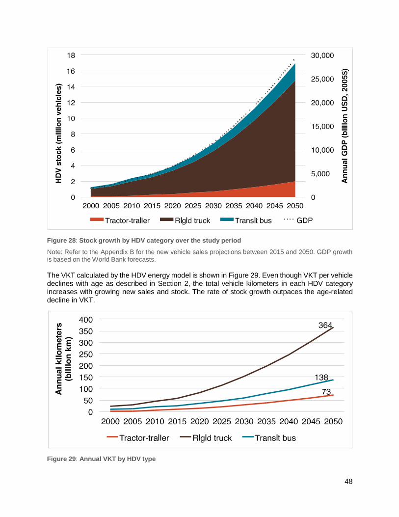
48

Figure 28: Stock growth by HDV category over the study period

Note: Refer to the Appendix B for the new vehicle sales projections between 2015 and 2050. GDP growth is based on the World Bank forecasts.

The VKT calculated by the HDV energy model is shown in Figure 29. Even though VKT per vehicle declines with age as described in Section 2, the total vehicle kilometers in each HDV category increases with growing new sales and stock. The rate of stock growth outpaces the age-related decline in VKT.

Figure 29: Annual VKT by HDV type

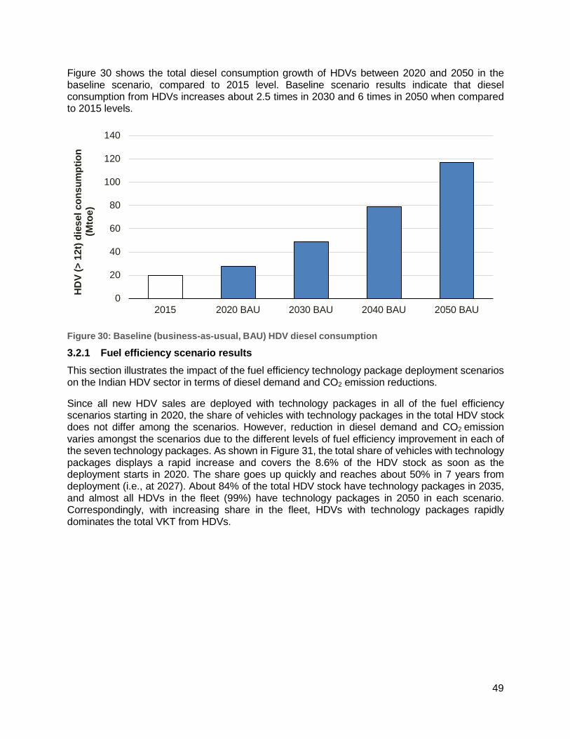
49

Figure 30 shows the total diesel consumption growth of HDVs between 2020 and 2050 in the baseline scenario, compared to 2015 level. Baseline scenario results indicate that diesel consumption from HDVs increases about 2.5 times in 2030 and 6 times in 2050 when compared to 2015 levels.

140

120

100

80

60

40

20

0 2015 2020 BAU 2030 BAU 2040 BAU 2050 BAU

Figure 30: Baseline (business-as-usual, BAU) HDV diesel consumption

3.2.1 Fuel efficiency scenario results

This section illustrates the impact of the fuel efficiency technology package deployment scenarios on the Indian HDV sector in terms of diesel demand and CO2 emission reductions.

Since all new HDV sales are deployed with technology packages in all of the fuel efficiency scenarios starting in 2020, the share of vehicles with technology packages in the total HDV stock does not differ among the scenarios. However, reduction in diesel demand and CO2 emission varies amongst the scenarios due to the different levels of fuel efficiency improvement in each of the seven technology packages. As shown in Figure 31, the total share of vehicles with technology packages displays a rapid increase and covers the 8.6% of the HDV stock as soon as the deployment starts in 2020. The share goes up quickly and reaches about 50% in 7 years from deployment (i.e., at 2027). About 84% of the total HDV stock have technology packages in 2035, and almost all HDVs in the fleet (99%) have technology packages in 2050 in each scenario. Correspondingly, with increasing share in the fleet, HDVs with technology packages rapidly dominates the total VKT from HDVs.

HD

V (

> 1

2t)

die

se

l co

nsu

mp

tio

n

(Mto

e)

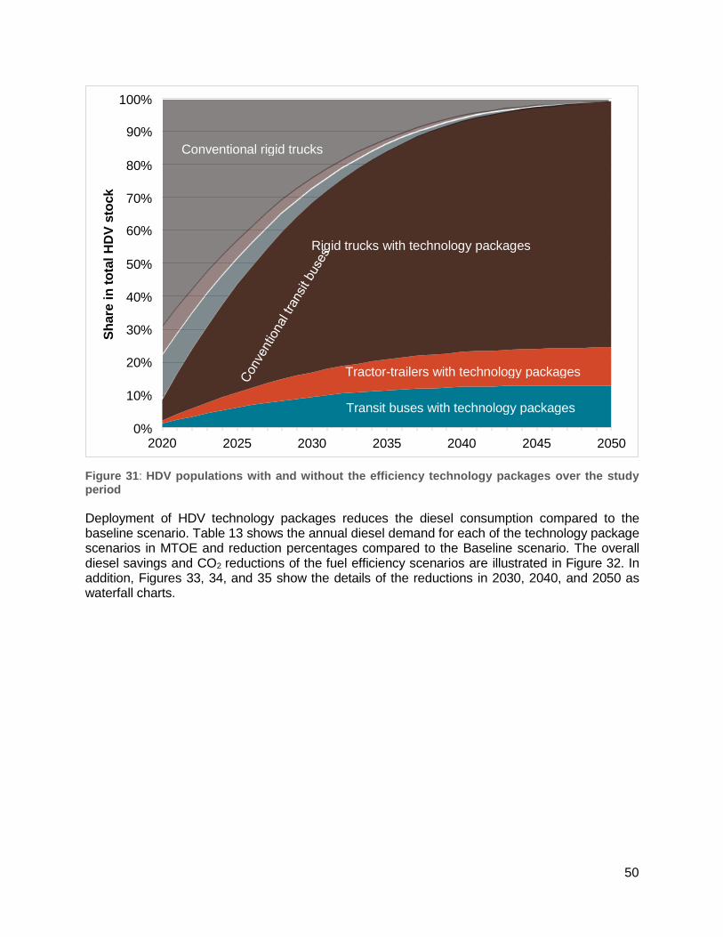
50

100%

90%

Conventional rigid trucks

80%

70%

60%

Rigid trucks with technology packages

50%

40%

30%

20%

Tractor-trailers with technology packages

10% Transit buses with technology packages

0% 2020 2025 2030 2035 2040 2045 2050

Figure 31: HDV populations with and without the efficiency technology packages over the study period

Deployment of HDV technology packages reduces the diesel consumption compared to the baseline scenario. Table 13 shows the annual diesel demand for each of the technology package scenarios in MTOE and reduction percentages compared to the Baseline scenario. The overall diesel savings and CO2 reductions of the fuel efficiency scenarios are illustrated in Figure 32. In addition, Figures 33, 34, and 35 show the details of the reductions in 2030, 2040, and 2050 as waterfall charts.

Sh

are

in

to

tal

HD

V s

tock

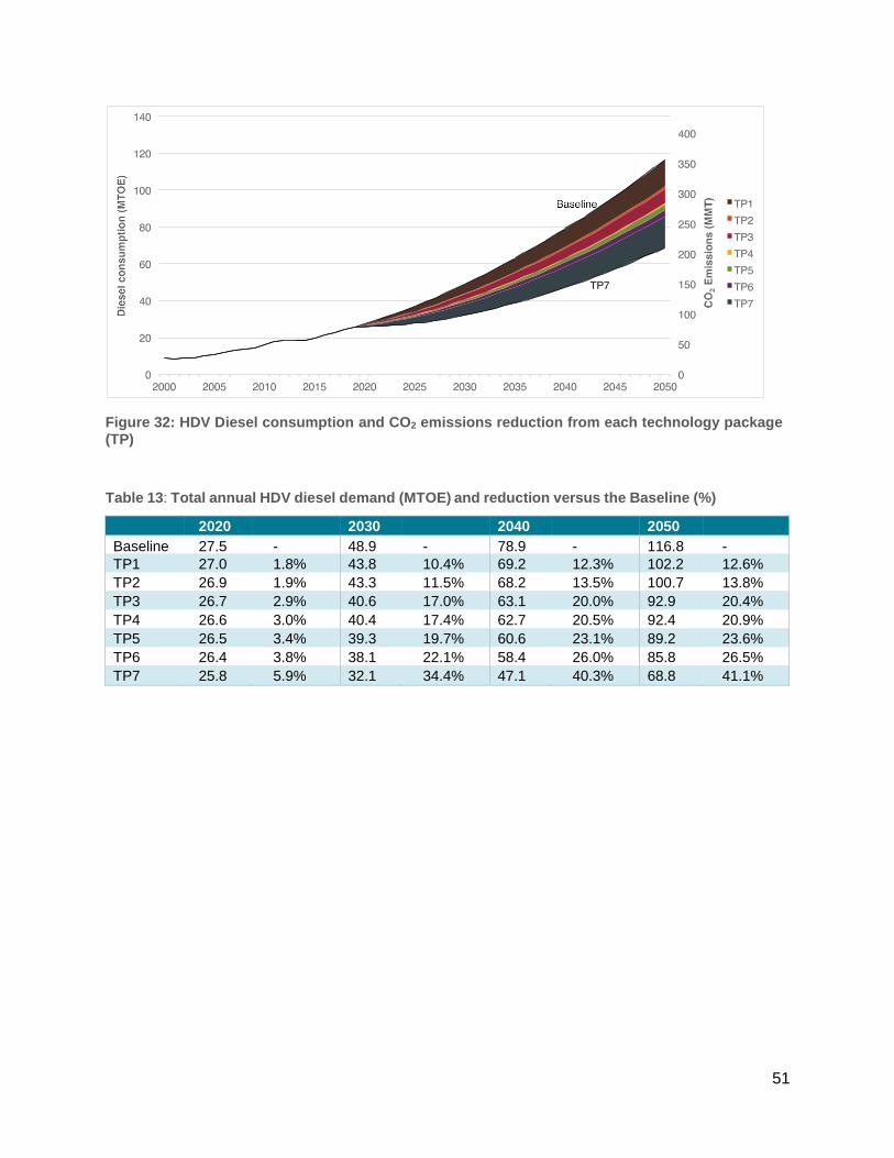
51

Figure 32: HDV Diesel consumption and CO2 emissions reduction from each technology package (TP)

Table 13: Total annual HDV diesel demand (MTOE) and reduction versus the Baseline (%)

2020 2030 2040 2050 Baseline 27.5 - 48.9 - 78.9 - 116.8 - TP1 27.0 1.8% 43.8 10.4% 69.2 12.3% 102.2 12.6% TP2 26.9 1.9% 43.3 11.5% 68.2 13.5% 100.7 13.8% TP3 26.7 2.9% 40.6 17.0% 63.1 20.0% 92.9 20.4% TP4 26.6 3.0% 40.4 17.4% 62.7 20.5% 92.4 20.9% TP5 26.5 3.4% 39.3 19.7% 60.6 23.1% 89.2 23.6% TP6 26.4 3.8% 38.1 22.1% 58.4 26.0% 85.8 26.5% TP7 25.8 5.9% 32.1 34.4% 47.1 40.3% 68.8 41.1%

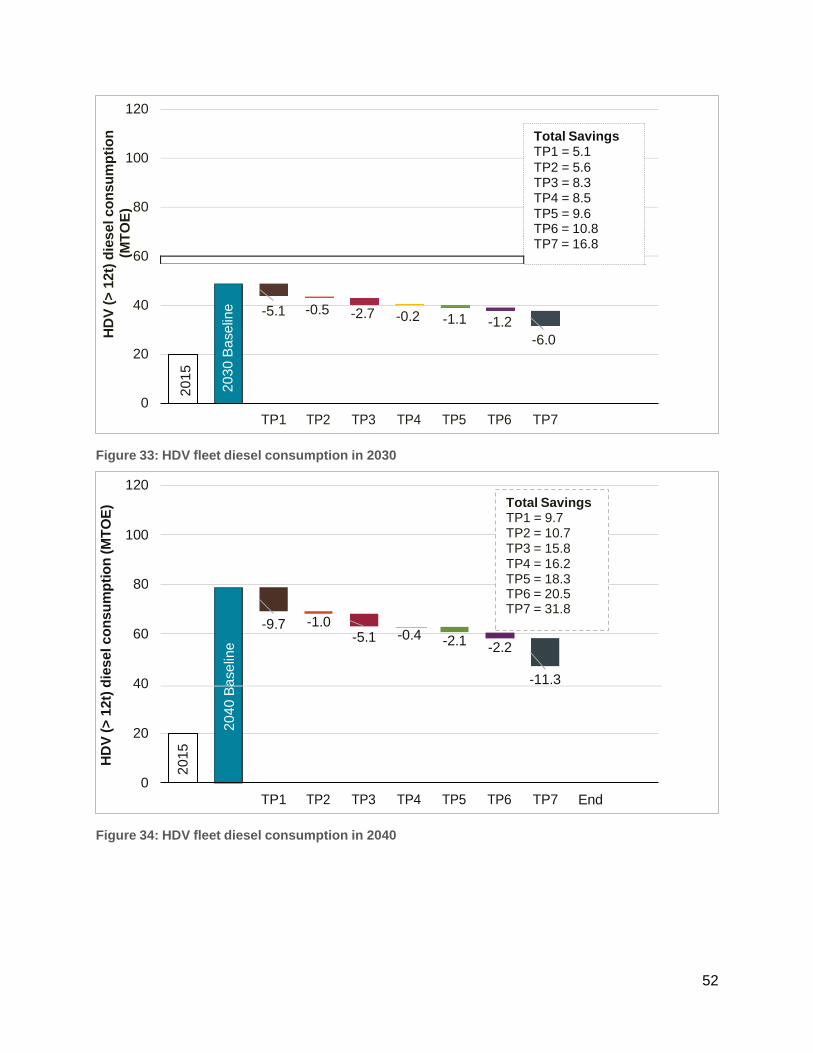
52

End

120

100

80

60

40 -5.1 -0.5 -2.7 -0.2 -1.1 -1.2

-6.0 20

0


120

100

80

Total Savings TP1 = 9.7 TP2 = 10.7 TP3 = 15.8 TP4 = 16.2 TP5 = 18.3 TP6 = 20.5 TP7 = 31.8

-1.0 60

-9.7 -5.1

-0.4 -2.1

-2.2

40 -11.3

20

0

TP1 TP2 TP3 TP4 TP5 TP6 TP7 End

Figure 33: HDV fleet diesel consumption in 2030


Total Savings TP1 = 5.1

TP2 = 5.6 TP3 = 8.3 TP4 = 8.5

TP5 = 9.6 TP6 = 10.8 TP7 = 16.8

HD

V (

> 1

2t)

die

se

l co

nsu

mp

tio

n (

MT

OE

) H

DV

(>

12

t) d

ies

el co

nsu

mp

tio

n

(MT

OE

)

20

15

20

30

Ba

se

line

20

40

Ba

se

line

20

15

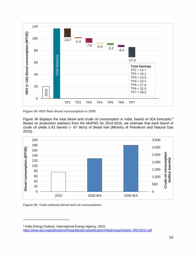
53

End

120

100 -14.7 -1.4

-7.8

-0.5 80

-3.2 -3.4

60

40

20

-17.0

Total Savings TP1 = 14.7 TP2 = 16.1 TP3 = 23.9 TP4 = 24.4 TP5 = 27.6 TP6 = 31.0 TP7 = 48.0

0



Figure 36 displays the total diesel and crude oil consumption in India, based on IEA forecasts.6

Based on production statistics from the MoPNG for 2014-2015, we estimate that each barrel of crude oil yields 0.42 barrels (~ 67 liters) of diesel fuel (Ministry of Petroleum and Natural Gas 2016).

200

180

160

140

120

100

80

60

40

20

0

2015 2030 IEA 2040 IEA

3,500

3,000

2,500

2,000

1,500

1,000

500

0

Figure 36: Total national diesel and oil consumption

6 India Energy Outlook, International Energy Agency. 2015 https://www.iea.org/publications/freepublications/publication/IndiaEnergyOutlook_WEO2015.pdf

HD

V (

> 1

2t)

die

se

l co

nsu

mp

tio

n (

MT

OE

)

20

15

Die

se

l co

nsu

mp

tio

n (

MT

OE

)

Cru

de

oil c

on

su

mp

tio

n

(millio

n b

arr

els

)

20

50

Ba

se

line

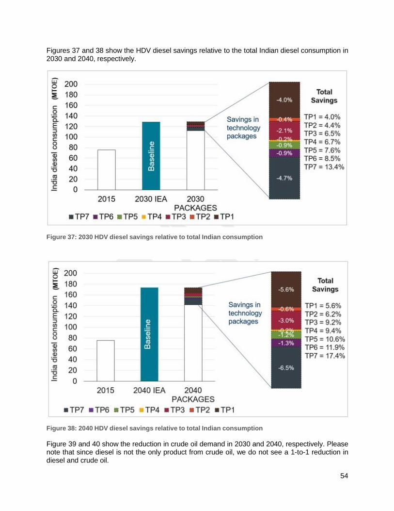
https://www.iea.org/publications/freepublications/publication/IndiaEnergyOutlook_WEO2015.pdf

https://www.iea.org/publications/freepublications/publication/IndiaEnergyOutlook_WEO2015.pdf

54

Figures 37 and 38 show the HDV diesel savings relative to the total Indian diesel consumption in 2030 and 2040, respectively.

Figure 37: 2030 HDV diesel savings relative to total Indian consumption

Figure 38: 2040 HDV diesel savings relative to total Indian consumption

Figure 39 and 40 show the reduction in crude oil demand in 2030 and 2040, respectively. Please note that since diesel is not the only product from crude oil, we do not see a 1-to-1 reduction in diesel and crude oil.

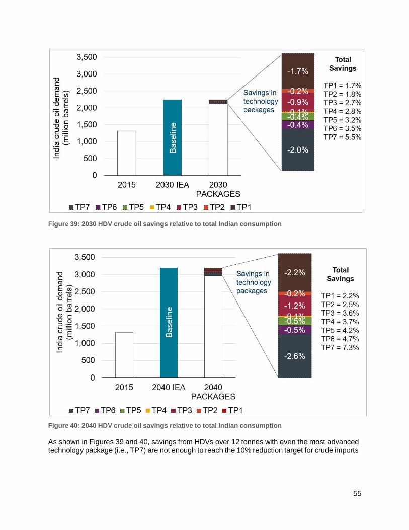
55

Figure 39: 2030 HDV crude oil savings relative to total Indian consumption

Figure 40: 2040 HDV crude oil savings relative to total Indian consumption

As shown in Figures 39 and 40, savings from HDVs over 12 tonnes with even the most advanced technology package (i.e., TP7) are not enough to reach the 10% reduction target for crude imports

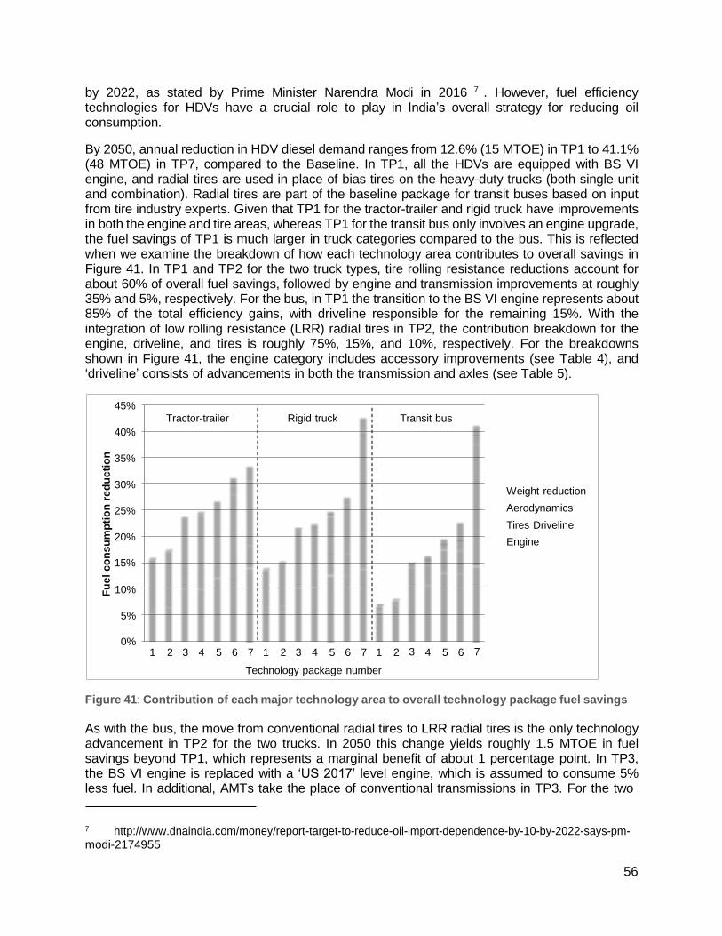
56

45%


40%

35%

30%

25%

20%

15%

Weight reduction

Aerodynamics

Tires Driveline

Engine

10%

5%

0%

1 2 3 4 5 6 7 1 2 3 4 5 6 7 1 2 3 4 5 6 7

Technology package number

by 2022, as stated by Prime Minister Narendra Modi in 2016 7 . However, fuel efficiency technologies for HDVs have a crucial role to play in India’s overall strategy for reducing oil consumption.

By 2050, annual reduction in HDV diesel demand ranges from 12.6% (15 MTOE) in TP1 to 41.1% (48 MTOE) in TP7, compared to the Baseline. In TP1, all the HDVs are equipped with BS VI engine, and radial tires are used in place of bias tires on the heavy-duty trucks (both single unit and combination). Radial tires are part of the baseline package for transit buses based on input from tire industry experts. Given that TP1 for the tractor-trailer and rigid truck have improvements in both the engine and tire areas, whereas TP1 for the transit bus only involves an engine upgrade, the fuel savings of TP1 is much larger in truck categories compared to the bus. This is reflected when we examine the breakdown of how each technology area contributes to overall savings in Figure 41. In TP1 and TP2 for the two truck types, tire rolling resistance reductions account for about 60% of overall fuel savings, followed by engine and transmission improvements at roughly 35% and 5%, respectively. For the bus, in TP1 the transition to the BS VI engine represents about 85% of the total efficiency gains, with driveline responsible for the remaining 15%. With the integration of low rolling resistance (LRR) radial tires in TP2, the contribution breakdown for the engine, driveline, and tires is roughly 75%, 15%, and 10%, respectively. For the breakdowns shown in Figure 41, the engine category includes accessory improvements (see Table 4), and ‘driveline’ consists of advancements in both the transmission and axles (see Table 5).

Figure 41: Contribution of each major technology area to overall technology package fuel savings

As with the bus, the move from conventional radial tires to LRR radial tires is the only technology advancement in TP2 for the two trucks. In 2050 this change yields roughly 1.5 MTOE in fuel savings beyond TP1, which represents a marginal benefit of about 1 percentage point. In TP3, the BS VI engine is replaced with a ‘US 2017’ level engine, which is assumed to consume 5% less fuel. In additional, AMTs take the place of conventional transmissions in TP3. For the two

7 http://www.dnaindia.com/money/report-target-to-reduce-oil-import-dependence-by-10-by-2022-says-pm- modi-2174955

Fu

el

co

ns

um

pti

on

re

du

cti

on

http://www.dnaindia.com/money/report-target-to-reduce-oil-import-dependence-by-10-by-2022-says-pm-

57

trucks in Figure 41, there is an increased contribution of engines (~ 40-50%) and driveline (~ 15%) in TP3, with tires accounting for the remaining 35-45% of overall fuel consumption reduction. For the buses, TP3 fuel savings contribution roughly breaks down as follows: engines – 70%; driveline – 25%; tires – 5%. The engine and transmission technologies of TP3 result in roughly 6.6% (i.e., 7.7 MTOE) of additional diesel savings compared to TP2 in 2050.

TP4 involves a moderate decrease in aerodynamic drag (10% reduction in CD) for the two trucks and a 1% reduction in curb weight for the bus, and this results in 0.6 MTOE of fuel savings beyond TP3. We see in Figure 41 that the respective contributions of aerodynamic and weight reduction improvements are fairly small at 5% or less. TP5 marks the introduction of the ‘US 2020+’ engine, which is nearly 3% more efficient than the ‘US 2017’ engine and 12.5% more efficient than the baseline BS IV. In addition, TP5 for the two trucks includes another step down in aerodynamic drag (20% reduction in CD versus the baseline) and a 1% reduction in vehicle empty weight. The bus also gets a ‘US 2020+’ engine in TP5, but has a further reduction in weight (2.5% versus the baseline) instead of aerodynamic improvements. The marginal impact of TP5 is an additional fuel reduction of 3.1 MTOE in 2050, and this is primarily driven by the transition to the ‘US 2020+’ engine, as aerodynamics and weight reduction still represent less than 5% of overall savings, despite the incremental advances in both of these areas. With TP6, there is the transition to advanced LRR tires, which provide a 10% reduction in CRR beyond LRR tires, as well as the introduction of tire pressure management systems. Maintaining proper air pressure in tires is assumed to provide 1% overall fuel savings for each of the three HDV types. For the tractor-trailer, there is another 10 percentage points of reduction in CD (30% total CD reduction versus the baseline) in TP6 that represents aerodynamic interventions on the trailer in addition to the tractor truck. TP6 also ratchets down in the weight reduction category: 2.5% versus the baseline for the trucks and 5% for the bus. Together, TP6 results in additional diesel savings of 3.4 MTOE in 2050.

In the most aggressive technology package, TP7, we reach the most efficient level of engine technology, which consumes 15% less fuel than the baseline BS IV engine. Moreover, for the rigid truck and bus, which are assumed to have significant portions of driving in stop-and-go urban conditions, we introduce a hybrid-electric system. The hybrid system is by far the most impactful individual technology and is assumed to provide 20% and 25% fuel savings in the rigid truck and bus, respectively. As shown in Figure 41, the increase in the ‘driveline’ portion is almost entirely responsible for outsize increase in total fuel reduction in TP7 for these two vehicle types. Finally, TP7 moves to a 5% weight reduction for the two trucks and 7.5% for the bus. With the fuel savings surge provided mostly by the introduction of hybrid vehicles, TP7 generates 17.0 MTOE of additional diesel savings.

Figure 42 illustrates the cost-effectiveness of each of the five major technology areas in terms of costs per percent reduction in fuel consumption for each of the three vehicle types across the seven technology packages. Across the three vehicle types, tire technologies provide the most cost-effective fuel savings, ranging from approximately 0.1 – 0.4 lakh/[% reduction]. The transition to radial tires and the further reduction in rolling resistance encompassed in TP1 through TP5 is particularly cost-effective, with values around 0.1 lakh/[% reduction]. Integration of tire pressure management systems in TP6 and TP7 bumps this range up to 0.2 – 0.4 lakh/[% reduction].

Engine technologies rank next after tires in terms of cost-effectiveness across all of the technology packages. Enhancements in engine efficiency and accessory loads yield savings for between 0.3 – 0.4 lakh/[% reduction].

Following engines, the next most cost-effective technology area is the transmission and axles (“Driveline” in the figure 42). Prior to the introduction of AMTs in TP3, TP1 and TP2 have improvements in axle efficiency and lubrication, which yield roughly 1% fuel savings for all three

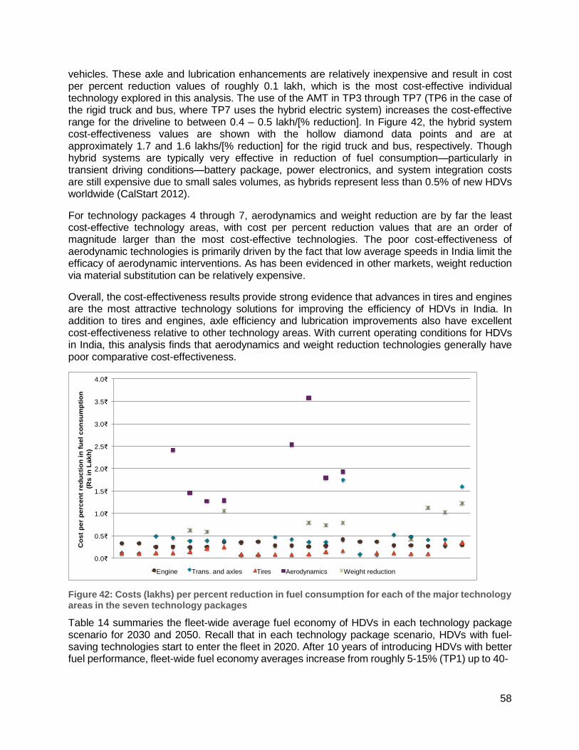
58

4.0₹

3.5₹

3.0₹

2.5₹

2.0₹

1.5₹

1.0₹

0.5₹

0.0₹

Engine Trans. and axles Tires Aerodynamics Weight reduction

vehicles. These axle and lubrication enhancements are relatively inexpensive and result in cost per percent reduction values of roughly 0.1 lakh, which is the most cost-effective individual technology explored in this analysis. The use of the AMT in TP3 through TP7 (TP6 in the case of the rigid truck and bus, where TP7 uses the hybrid electric system) increases the cost-effective range for the driveline to between 0.4 – 0.5 lakh/[% reduction]. In Figure 42, the hybrid system cost-effectiveness values are shown with the hollow diamond data points and are at approximately 1.7 and 1.6 lakhs/[% reduction] for the rigid truck and bus, respectively. Though hybrid systems are typically very effective in reduction of fuel consumption—particularly in transient driving conditions—battery package, power electronics, and system integration costs are still expensive due to small sales volumes, as hybrids represent less than 0.5% of new HDVs worldwide (CalStart 2012).

For technology packages 4 through 7, aerodynamics and weight reduction are by far the least cost-effective technology areas, with cost per percent reduction values that are an order of magnitude larger than the most cost-effective technologies. The poor cost-effectiveness of aerodynamic technologies is primarily driven by the fact that low average speeds in India limit the efficacy of aerodynamic interventions. As has been evidenced in other markets, weight reduction via material substitution can be relatively expensive.

Overall, the cost-effectiveness results provide strong evidence that advances in tires and engines are the most attractive technology solutions for improving the efficiency of HDVs in India. In addition to tires and engines, axle efficiency and lubrication improvements also have excellent cost-effectiveness relative to other technology areas. With current operating conditions for HDVs in India, this analysis finds that aerodynamics and weight reduction technologies generally have poor comparative cost-effectiveness.

Figure 42: Costs (lakhs) per percent reduction in fuel consumption for each of the major technology areas in the seven technology packages

Table 14 summaries the fleet-wide average fuel economy of HDVs in each technology package scenario for 2030 and 2050. Recall that in each technology package scenario, HDVs with fuel- saving technologies start to enter the fleet in 2020. After 10 years of introducing HDVs with better fuel performance, fleet-wide fuel economy averages increase from roughly 5-15% (TP1) up to 40-

Co

st

pe

r p

erc

en

t re

du

cti

on

in

fu

el

co

ns

um

pti

on

(Rs

in

La

kh

)

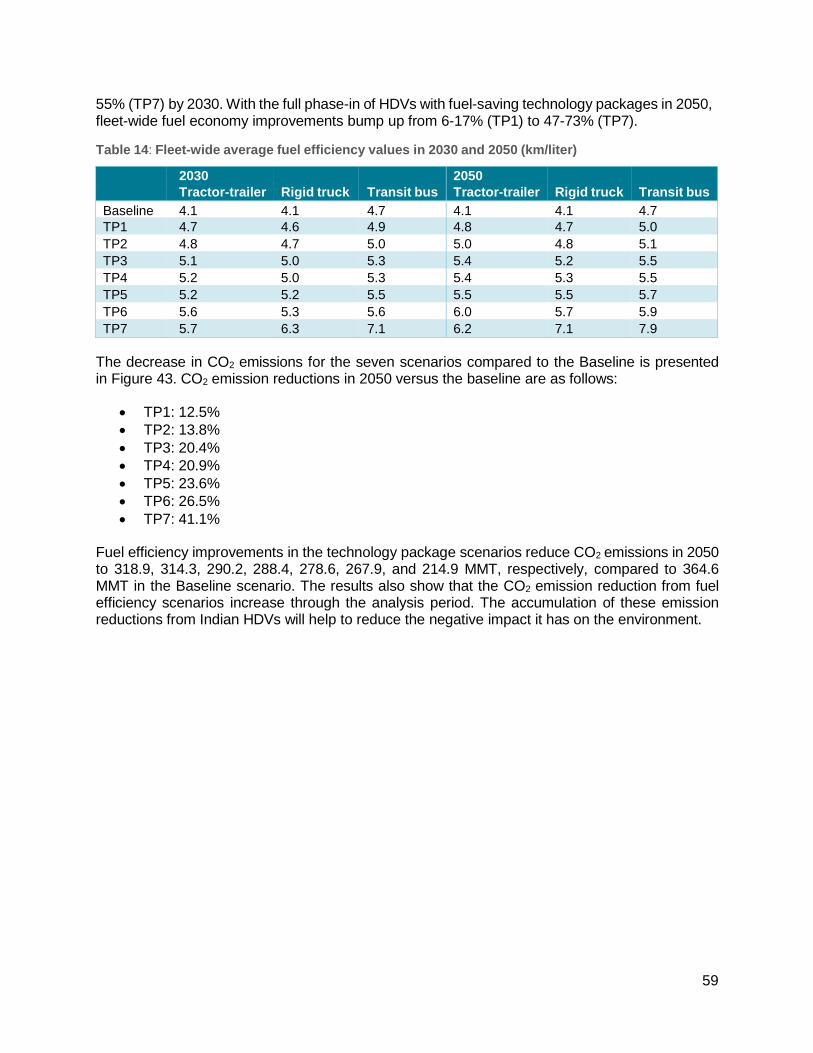
59

55% (TP7) by 2030. With the full phase-in of HDVs with fuel-saving technology packages in 2050, fleet-wide fuel economy improvements bump up from 6-17% (TP1) to 47-73% (TP7).

Table 14: Fleet-wide average fuel efficiency values in 2030 and 2050 (km/liter)

2030 2050 Tractor-trailer Rigid truck Transit bus Tractor-trailer Rigid truck Transit bus

Baseline 4.1 4.1 4.7 4.1 4.1 4.7 TP1 4.7 4.6 4.9 4.8 4.7 5.0 TP2 4.8 4.7 5.0 5.0 4.8 5.1 TP3 5.1 5.0 5.3 5.4 5.2 5.5 TP4 5.2 5.0 5.3 5.4 5.3 5.5 TP5 5.2 5.2 5.5 5.5 5.5 5.7 TP6 5.6 5.3 5.6 6.0 5.7 5.9 TP7 5.7 6.3 7.1 6.2 7.1 7.9

The decrease in CO2 emissions for the seven scenarios compared to the Baseline is presented in Figure 43. CO2 emission reductions in 2050 versus the baseline are as follows:

TP1: 12.5%

TP2: 13.8%

TP3: 20.4%

TP4: 20.9%

TP5: 23.6%

TP6: 26.5%

TP7: 41.1%

Fuel efficiency improvements in the technology package scenarios reduce CO2 emissions in 2050 to 318.9, 314.3, 290.2, 288.4, 278.6, 267.9, and 214.9 MMT, respectively, compared to 364.6 MMT in the Baseline scenario. The results also show that the CO2 emission reduction from fuel efficiency scenarios increase through the analysis period. The accumulation of these emission reductions from Indian HDVs will help to reduce the negative impact it has on the environment.

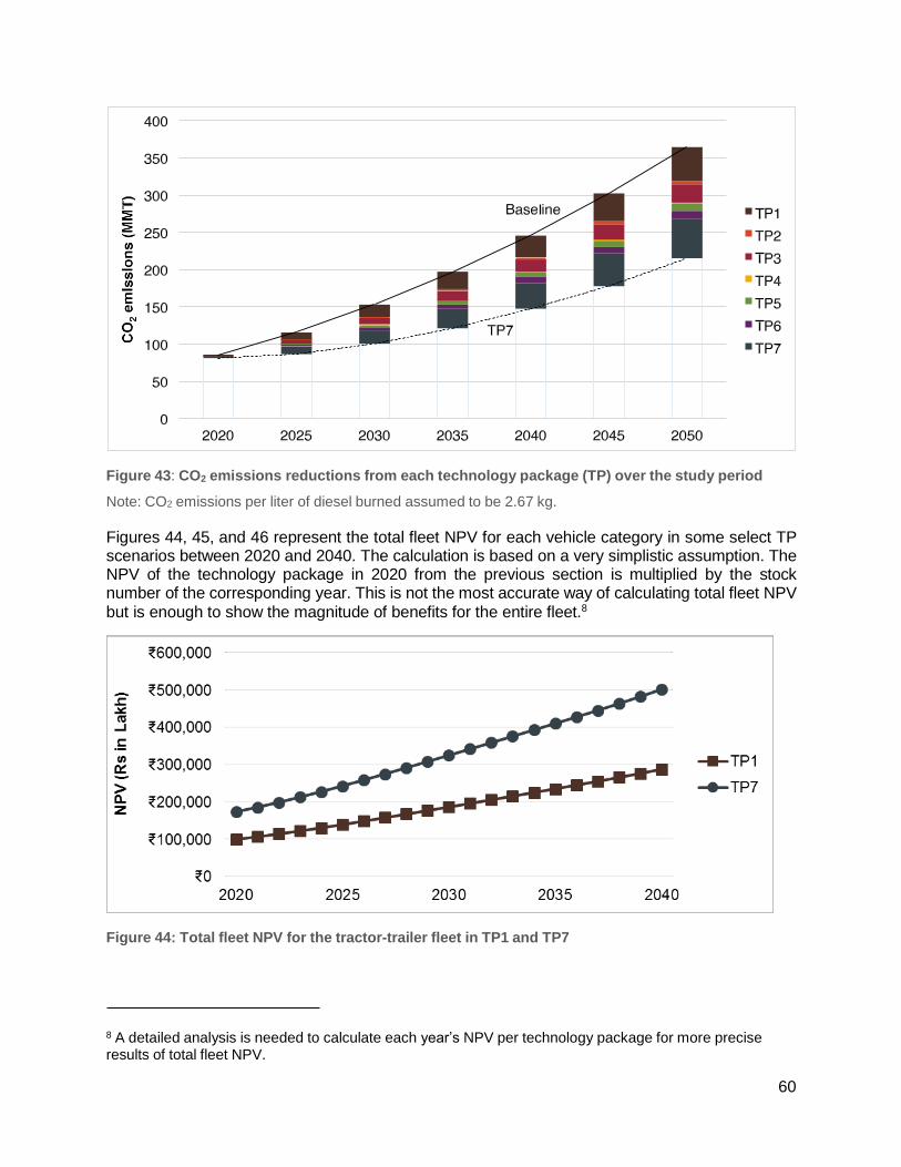
60

Figure 43: CO2 emissions reductions from each technology package (TP) over the study period

Note: CO2 emissions per liter of diesel burned assumed to be 2.67 kg.

Figures 44, 45, and 46 represent the total fleet NPV for each vehicle category in some select TP scenarios between 2020 and 2040. The calculation is based on a very simplistic assumption. The NPV of the technology package in 2020 from the previous section is multiplied by the stock number of the corresponding year. This is not the most accurate way of calculating total fleet NPV

but is enough to show the magnitude of benefits for the entire fleet.8

Figure 44: Total fleet NPV for the tractor-trailer fleet in TP1 and TP7

8 A detailed analysis is needed to calculate each year’s NPV per technology package for more precise results of total fleet NPV.

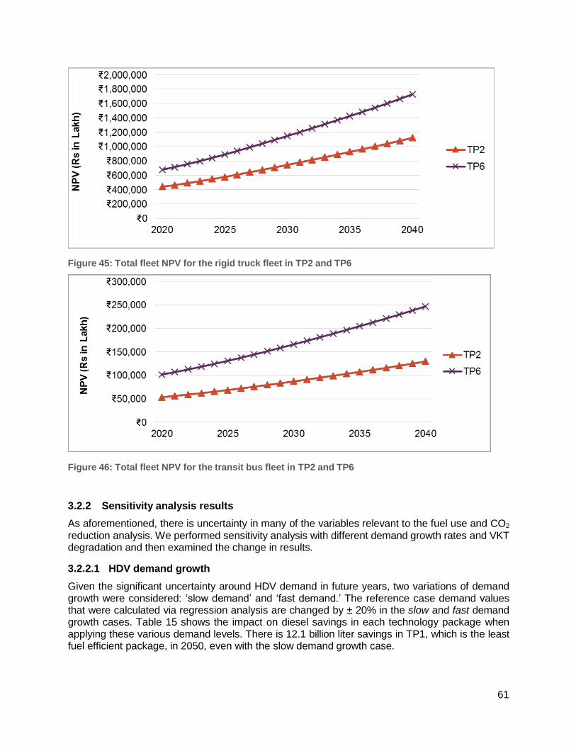
61

Figure 45: Total fleet NPV for the rigid truck fleet in TP2 and TP6

Figure 46: Total fleet NPV for the transit bus fleet in TP2 and TP6

3.2.2 Sensitivity analysis results

As aforementioned, there is uncertainty in many of the variables relevant to the fuel use and CO2

reduction analysis. We performed sensitivity analysis with different demand growth rates and VKT degradation and then examined the change in results.

3.2.2.1 HDV demand growth

Given the significant uncertainty around HDV demand in future years, two variations of demand growth were considered: ‘slow demand’ and ‘fast demand.’ The reference case demand values that were calculated via regression analysis are changed by ± 20% in the slow and fast demand growth cases. Table 15 shows the impact on diesel savings in each technology package when applying these various demand levels. There is 12.1 billion liter savings in TP1, which is the least fuel efficient package, in 2050, even with the slow demand growth case.

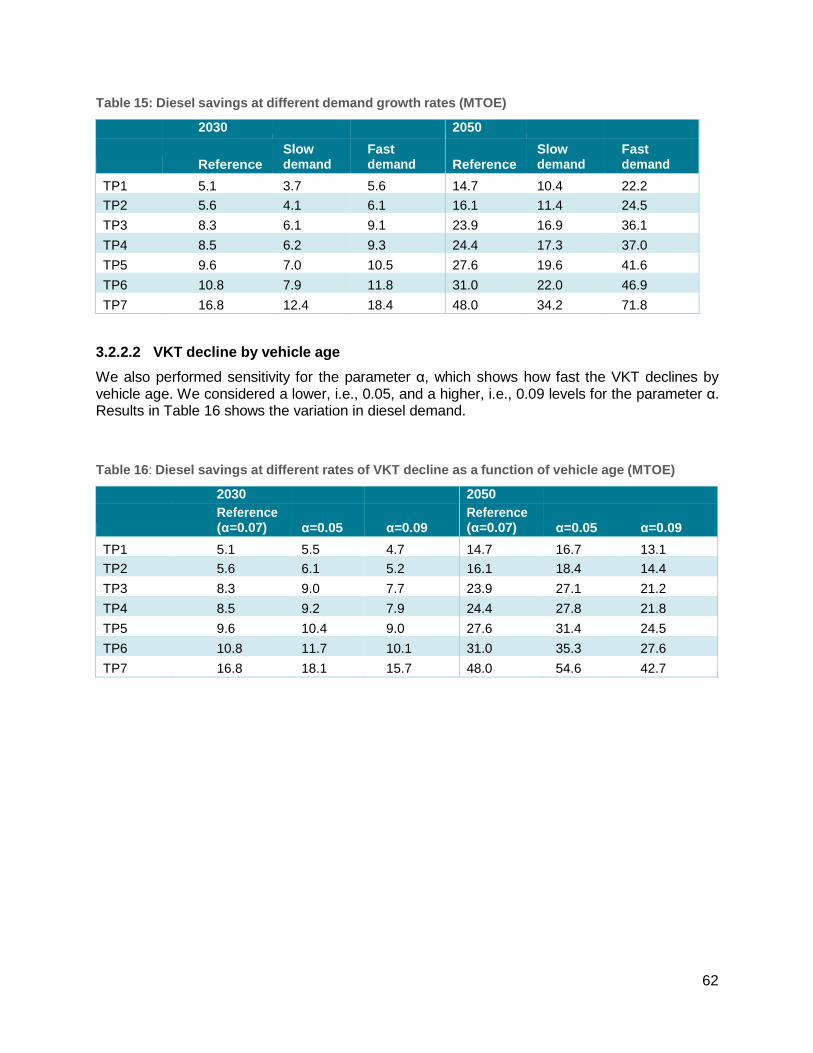
62

Table 15: Diesel savings at different demand growth rates (MTOE)

2030 2050

Reference

Slow demand

Fast demand

Reference

Slow demand

Fast demand

TP1 5.1 3.7 5.6 14.7 10.4 22.2

TP2 5.6 4.1 6.1 16.1 11.4 24.5

TP3 8.3 6.1 9.1 23.9 16.9 36.1

TP4 8.5 6.2 9.3 24.4 17.3 37.0

TP5 9.6 7.0 10.5 27.6 19.6 41.6

TP6 10.8 7.9 11.8 31.0 22.0 46.9

TP7 16.8 12.4 18.4 48.0 34.2 71.8

3.2.2.2 VKT decline by vehicle age

We also performed sensitivity for the parameter α, which shows how fast the VKT declines by vehicle age. We considered a lower, i.e., 0.05, and a higher, i.e., 0.09 levels for the parameter α. Results in Table 16 shows the variation in diesel demand.

Table 16: Diesel savings at different rates of VKT decline as a function of vehicle age (MTOE)

2030 2050 Reference

(α=0.07) α=0.05

α=0.09

Reference (α=0.07)

α=0.05

α=0.09

TP1 5.1 5.5 4.7 14.7 16.7 13.1

TP2 5.6 6.1 5.2 16.1 18.4 14.4

TP3 8.3 9.0 7.7 23.9 27.1 21.2

TP4 8.5 9.2 7.9 24.4 27.8 21.8

TP5 9.6 10.4 9.0 27.6 31.4 24.5

TP6 10.8 11.7 10.1 31.0 35.3 27.6

TP7 16.8 18.1 15.7 48.0 54.6 42.7

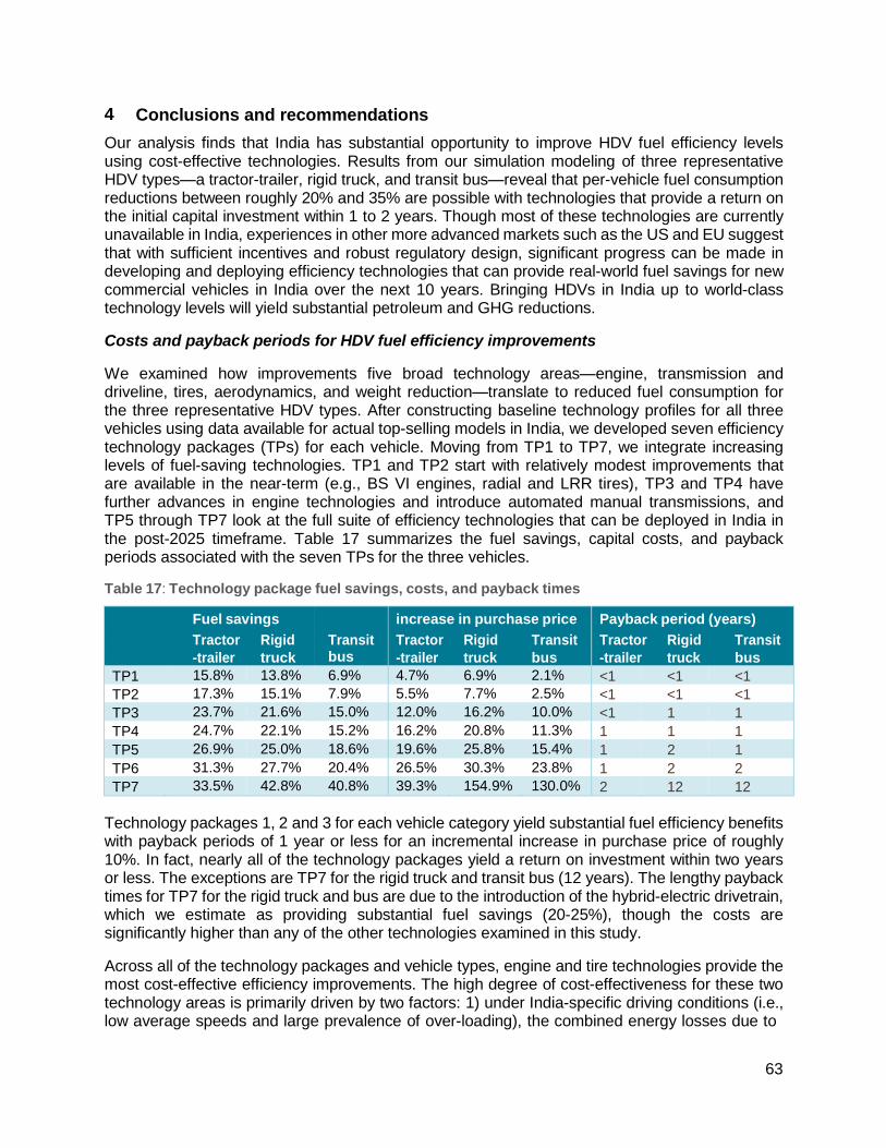
63

4 Conclusions and recommendations

Our analysis finds that India has substantial opportunity to improve HDV fuel efficiency levels using cost-effective technologies. Results from our simulation modeling of three representative HDV types—a tractor-trailer, rigid truck, and transit bus—reveal that per-vehicle fuel consumption reductions between roughly 20% and 35% are possible with technologies that provide a return on the initial capital investment within 1 to 2 years. Though most of these technologies are currently unavailable in India, experiences in other more advanced markets such as the US and EU suggest that with sufficient incentives and robust regulatory design, significant progress can be made in developing and deploying efficiency technologies that can provide real-world fuel savings for new commercial vehicles in India over the next 10 years. Bringing HDVs in India up to world-class technology levels will yield substantial petroleum and GHG reductions.

Costs and payback periods for HDV fuel efficiency improvements

We examined how improvements five broad technology areas—engine, transmission and driveline, tires, aerodynamics, and weight reduction—translate to reduced fuel consumption for the three representative HDV types. After constructing baseline technology profiles for all three vehicles using data available for actual top-selling models in India, we developed seven efficiency technology packages (TPs) for each vehicle. Moving from TP1 to TP7, we integrate increasing levels of fuel-saving technologies. TP1 and TP2 start with relatively modest improvements that are available in the near-term (e.g., BS VI engines, radial and LRR tires), TP3 and TP4 have further advances in engine technologies and introduce automated manual transmissions, and TP5 through TP7 look at the full suite of efficiency technologies that can be deployed in India in the post-2025 timeframe. Table 17 summarizes the fuel savings, capital costs, and payback periods associated with the seven TPs for the three vehicles.

Table 17: Technology package fuel savings, costs, and payback times

Fuel savings

Tractor Rigid

-trailer truck

Transit bus

increase in purchase price

Tractor Rigid Transit

-trailer truck bus

Payback period (years)

Tractor Rigid Transit

-trailer truck bus TP1 15.8% 13.8% 6.9% 4.7% 6.9% 2.1% <1 <1 <1 TP2 17.3% 15.1% 7.9% 5.5% 7.7% 2.5% <1 <1 <1 TP3 23.7% 21.6% 15.0% 12.0% 16.2% 10.0% <1 1 1 TP4 24.7% 22.1% 15.2% 16.2% 20.8% 11.3% 1 1 1 TP5 26.9% 25.0% 18.6% 19.6% 25.8% 15.4% 1 2 1 TP6 31.3% 27.7% 20.4% 26.5% 30.3% 23.8% 1 2 2 TP7 33.5% 42.8% 40.8% 39.3% 154.9% 130.0% 2 12 12

Technology packages 1, 2 and 3 for each vehicle category yield substantial fuel efficiency benefits with payback periods of 1 year or less for an incremental increase in purchase price of roughly 10%. In fact, nearly all of the technology packages yield a return on investment within two years or less. The exceptions are TP7 for the rigid truck and transit bus (12 years). The lengthy payback times for TP7 for the rigid truck and bus are due to the introduction of the hybrid-electric drivetrain, which we estimate as providing substantial fuel savings (20-25%), though the costs are significantly higher than any of the other technologies examined in this study.

Across all of the technology packages and vehicle types, engine and tire technologies provide the most cost-effective efficiency improvements. The high degree of cost-effectiveness for these two technology areas is primarily driven by two factors: 1) under India-specific driving conditions (i.e., low average speeds and large prevalence of over-loading), the combined energy losses due to

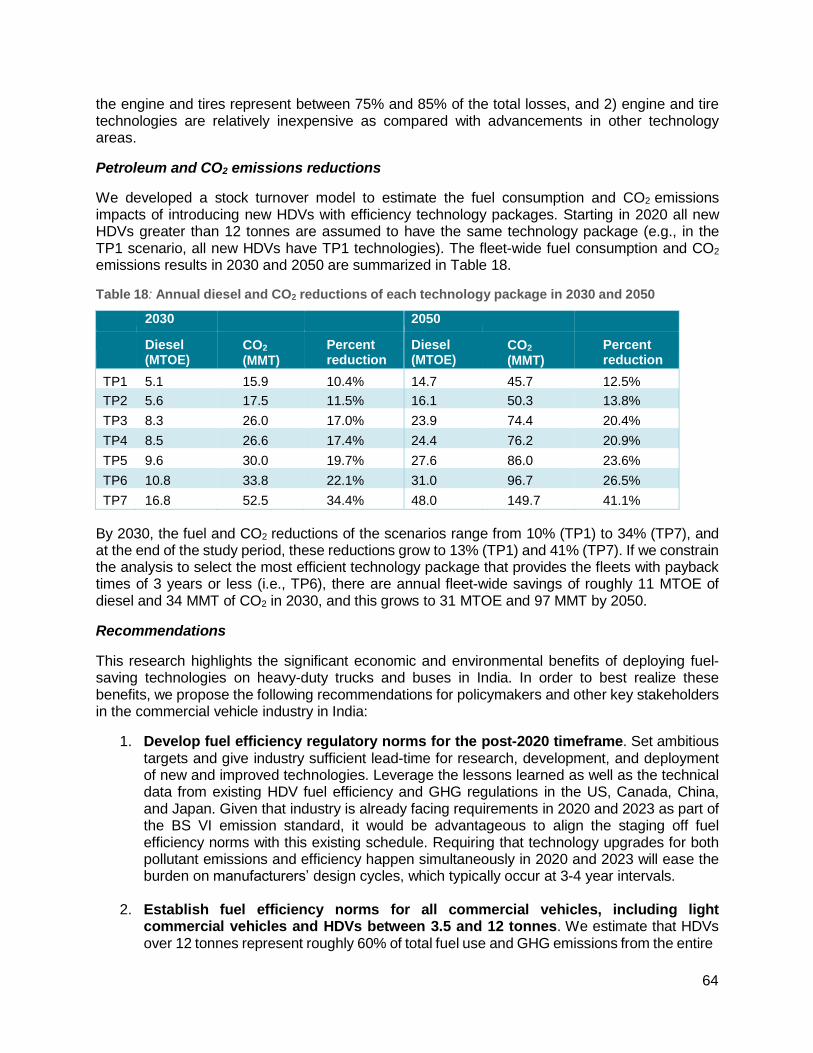
64

the engine and tires represent between 75% and 85% of the total losses, and 2) engine and tire technologies are relatively inexpensive as compared with advancements in other technology areas.

Petroleum and CO2 emissions reductions

We developed a stock turnover model to estimate the fuel consumption and CO2 emissions impacts of introducing new HDVs with efficiency technology packages. Starting in 2020 all new HDVs greater than 12 tonnes are assumed to have the same technology package (e.g., in the TP1 scenario, all new HDVs have TP1 technologies). The fleet-wide fuel consumption and CO2

emissions results in 2030 and 2050 are summarized in Table 18.

Table 18: Annual diesel and CO2 reductions of each technology package in 2030 and 2050

2030 2050

Diesel (MTOE)

CO2

(MMT) Percent reduction

Diesel (MTOE)

CO2

(MMT) Percent reduction

TP1 5.1 15.9 10.4% 14.7 45.7 12.5%

TP2 5.6 17.5 11.5% 16.1 50.3 13.8%

TP3 8.3 26.0 17.0% 23.9 74.4 20.4%

TP4 8.5 26.6 17.4% 24.4 76.2 20.9%

TP5 9.6 30.0 19.7% 27.6 86.0 23.6%

TP6 10.8 33.8 22.1% 31.0 96.7 26.5%

TP7 16.8 52.5 34.4% 48.0 149.7 41.1%

By 2030, the fuel and CO2 reductions of the scenarios range from 10% (TP1) to 34% (TP7), and at the end of the study period, these reductions grow to 13% (TP1) and 41% (TP7). If we constrain the analysis to select the most efficient technology package that provides the fleets with payback times of 3 years or less (i.e., TP6), there are annual fleet-wide savings of roughly 11 MTOE of diesel and 34 MMT of CO2 in 2030, and this grows to 31 MTOE and 97 MMT by 2050.

Recommendations

This research highlights the significant economic and environmental benefits of deploying fuel- saving technologies on heavy-duty trucks and buses in India. In order to best realize these benefits, we propose the following recommendations for policymakers and other key stakeholders in the commercial vehicle industry in India:

1. Develop fuel efficiency regulatory norms for the post-2020 timeframe. Set ambitious targets and give industry sufficient lead-time for research, development, and deployment of new and improved technologies. Leverage the lessons learned as well as the technical data from existing HDV fuel efficiency and GHG regulations in the US, Canada, China, and Japan. Given that industry is already facing requirements in 2020 and 2023 as part of the BS VI emission standard, it would be advantageous to align the staging off fuel efficiency norms with this existing schedule. Requiring that technology upgrades for both pollutant emissions and efficiency happen simultaneously in 2020 and 2023 will ease the burden on manufacturers’ design cycles, which typically occur at 3-4 year intervals.

2. Establish fuel efficiency norms for all commercial vehicles, including light commercial vehicles and HDVs between 3.5 and 12 tonnes. We estimate that HDVs over 12 tonnes represent roughly 60% of total fuel use and GHG emissions from the entire

65

HDV fleet—that is, all HDVs greater than 3.5 tonnes. With such a sizable contribution from trucks and buses less than 12 tonnes, we encourage regulators in India to pursue fuel efficiency norms for these smaller commercial vehicles as soon as possible. Our research in other markets suggests that comparable levels of cost-effective fuel efficiency improvements are available for this segment of the HDV fleet as well. In future research we will explore the technology opportunities for HDVs less than 12 tonnes in more detail.

3. Cultivate testing efforts for vehicles, engines, and component systems. The government of India, industry, and the research community should accelerate efforts to develop and implement testing campaigns that will provide the data that is critical to establishing more robust fuel efficiency norms that provide real-world benefits to fleets and society at large. Essential research includes:

Data logging of trucks and buses of various types and sizes to develop a suite of India- specific HDV drive cycles.

Surveys of fleets and analysis of payload data to determine average payloads by vehicle category.

Chassis dynamometer and PEMS testing of a wide range of trucks and buses over various drive cycles to better establish baseline fuel efficiency values and to support simulation model validation. Coastdown (and/or constant speed) testing is a requirement for developing the required chassis dynamometer inputs.

Engine dynamometer testing of top-selling engine sizes and power ratings over the BS IV and VI engine cycles. Determine the efficiency impacts of transitioning from BS IV to BS VI for a range of representative engines.

Testing of a broad range of bias and radial tires for rolling resistance and wet grip performance.

66

Acknowledgments

The authors are grateful to the Petroleum Conservation Research Association of the Ministry of Petroleum and Natural Gas for their support during this work. We are also grateful to our reviewers, Rashid Waraich, Nina Khanna, Rachel Muncrief, Felipe Rodriguez, Prashant Rawat, Sumant Kumar, Subrojit Pal, and Ravi Gadepalli for reviewing earlier drafts of this report.

References

Association of State Road Transport Undertakings (2012). Report of the Sub-Group on State Road Transport Undertakings Formed Under the Working Group on Road Transport Constituted by the Planning Commission. New Delhi, India.

Axis Bank India. (2016). "Commercial Vehicle & Construction Equipment Interest Rates." Retrieved October 26, 2016, from http://web2.axisbank.com/personal/loans/commercial-vehicle-and- construction-equipment-loans/fees-charges.aspx.

Bureau of Labor Statistics. (2013, August 28). "India's organized manufacturing sector: Average hourly compensation for all employees in manufacturing, selected economies and regions, 2000- 2010." Retrieved October 24, 2016, from http://www.bls.gov/fls/india.htm - Chart05.

California Air Resources Board. (2015, May 12). "EMFAC2014 Volume III - Technical Documentation." Retrieved October 24, 2016, from https://www.arb.ca.gov/msei/downloads/emfac2014/emfac2014-vol3-technical-documentation- 052015.pdf

CalStart (2012). Demand Assessment of First-Mover Hybrid and Electric Truck Fleets. Pasadena, CA.

Central Pollution Control Board. (2008). "Vehicular Exhaust: Emission Norms for Heavy Diesel Vehicles." Retrieved November 17, 2015, from http://cpcb.nic.in/Vehicular_Exhaust.php.

Clean Air Asia (2012). Development of Clean Fleet Bus Program for India. Pasig City, Philippines, Shakti Foundation.

Climate Action Tracker Partners (2016, November 2). "Cliamte Action Tracker: India." Retrieved November 21, 2016, from http://climateactiontracker.org/countries/india.

Committee on Assessment of Technologies and Approaches for Reducing the Fuel Consumption of Medium- and Heavy-Duty Vehicles - Phase Two (2014). Reducing the Fuel Consumption and Greenhouse Gas Emissions of Medium- and Heavy-Duty Vehicles, Phase Two - First Report. Washington, DC, National Research Council of the National Academies.

Committee to Assess Fuel Economy Technologies for Medium- and Heavy-Duty Vehicles (2010). Technologies and Approaches to Reducing the Fuel Consumption of Medium- and Heavy-Duty Vehicles. Washington, DC, National Research Council of the National Academies.

Delgado, O. (2016). Stage 3 China fuel consumption standard for commercial heavy-duty vehicles. Washington, DC, The International Council on Clean Transportation.

Delgado, O. and N. Lutsey (2015). Advanced Tractor-Trailer Efficiency Technology Potential in the 2020-2030 Timeframe. Washington, DC, The International Council on Clean Transportation.

Delucchi, M. A. (2011). Advanced-Vehicle Cost and Energy Use Model (AVCEM).

http://web2.axisbank.com/personal/loans/commercial-vehicle-and-construction-equipment-loans/fees-charges.aspx

http://web2.axisbank.com/personal/loans/commercial-vehicle-and-construction-equipment-loans/fees-charges.aspx

http://www.bls.gov/fls/india.htm#Chart05

https://www.arb.ca.gov/msei/downloads/emfac2014/emfac2014-vol3-technical-documentation-052015.pdf

https://www.arb.ca.gov/msei/downloads/emfac2014/emfac2014-vol3-technical-documentation-052015.pdf

http://cpcb.nic.in/Vehicular_Exhaust.php

http://climateactiontracker.org/countries/india

67

Dhiman, R. (2016). The impact of upcoming emissions legislation on the technology changes, cost and customer challenges. ICAT Powertrain Conference. Gurgaon, India, Escorts Agri Machinery.

Editorial Board of the Times of India (2014). Oil ministry to seek Cabinet nod on diesel deregulation. The Times of India. Delhi, India, Times Group.

Gibbs, N. (2015). Return of India's trucks. Automotive Manufacturing Solutions. London, United Kingdom, Ultima Media.

Goodyear Tire and Rubber Company. (2015). "Factors Affecting Truck Fuel Economy." Retrieved November 3, 2015, from http://www.goodyeartrucktires.com/resources/factors-fuel-economy.aspx

Gota, S., P. Bosu and S. K. Anthapur (2014). "Improving Fuel Efficiency and Reducing Carbon Emissions from Buses in India." Journal of Public Transportation 17(3): 3.

Heinz, S. (2001). Development of a World-wide Harmonised Heavy-duty Engine Emissions Test Cycle. Geneva, Switzlerland, ECE-GRPE WHDC Working Group.

Hill, N., S. Finnegan, J. Norris, C. Brannigan, D. Wynn, H. Baker and I. Skinner (2011). Reduction and Testing of Greenhouse Gas (GHG) Emissions from Heavy Duty Vehicles – Lot 1: Strategy. London, England, Ricardo-AEA.

International Council on Clean Transportation (2015). India Model v3s.xlsm. Washington, DC.

International Energy Agency (IEA) 2015. "India Energy Outlook. "… Retrieved December 1, 2016, from https://www.iea.org/publications/freepublications/publication/IndiaEnergyOutlook_WEO2015.pdf

International Institute for Sustainable Development (2013). The Impacts of India’s Diesel Price Reforms on the Trucking Industry. New Delhi, India.

Isaiah, D. (2013). AMT: the future of Indian truck transmissions? Automotive World. Penarth, United Kingdom.

Malik, J., Y. Karpate, A. Datta, S. Sharma and B. Sharpe (2016). Tire technologies and their impact on heavy-duty vehicle fuel efficiency in India. Delhi, India, The Energy and Resources Institute.

Meszler, D., N. Lutsey and O. Delgado (2015). Cost effectiveness of advanced efficiency technologies for long-haul tractor-trailers in the 2020-2030 timeframe. Washington, DC, The International Council on Clean Transportation.

Miller, J. (2016, April 4). "India: Heavy-duty emissions." Retrieved August 15, 2016, from http://transportpolicy.net/index.php?title=India:_Heavy-duty:_Emissions.

Ministry of Petroleum and Natural Gas. (2016, October 17). "Petroleum Prices." Retrieved October 18, 2016, from http://ppac.org.in/content/149_1_PricesPetroleum.aspx.

Ministry of Petroleum and Natural Gas (2016, August 17). "Petroleum Production." Retrieved November 21, 2016, from http://ppac.org.in/content/146_1_ProductionPetroleum.aspx

Ministry of Petroleum and Natural Gas. (2016, July 11). "Petroleum Consumption." Retrieved November 11, 2016, from http://ppac.org.in/content/147_1_ConsumptionPetroleum.aspx.

http://www.goodyeartrucktires.com/resources/factors-fuel-economy.aspx

https://www.iea.org/publications/freepublications/publication/IndiaEnergyOutlook_WEO2015

https://www.iea.org/publications/freepublications/publication/IndiaEnergyOutlook_WEO2015

http://transportpolicy.net/index.php?title=India%3A_Heavy-duty%3A_Emissions

http://ppac.org.in/content/149_1_PricesPetroleum.aspx

http://ppac.org.in/content/147_1_ConsumptionPetroleum.aspx

68

Ministry of Road Transport and Highways (MoRTH) (2015). Freight and Passenger Movement by Road Transport and Railways during 1999-2000 to 2011-12. New Delhi, India. Retrieved December 1, 2016, from https://data.gov.in/catalog/freight-and-passenger-movement-road-transport-and- railways

Ministry of Road Transport and Highways (2016). Review of the Performance of State Road Transport Undertakings (Passenger Services) for April 2014 to March 2015. New Delhi, India.

Ministry of Statistics and Programme Implementation. (2016). "Press Release: Consumer Price Index." Retrieved October 26, 2016, from http://mospi.nic.in/Mospi_New/upload/cpi_pr_12may16th.pdf

Nishimura, E. (2011). Assessing the Fuel Use and Greenhouse Gas Emissions of Future Light-Duty Vehicles in Japan. Masters, Massachusetts Institute of Technology.

Petroleum Planning and Analysis Cell and Nielsen (2013). All India Study on Sectoral Demand of Diesel and Petrol. Delhi, India, Ministry of Petroleum and Natural Gas.

Posada, F., S. Chambliss and K. Blumberg (2016). Costs of emission reduction technologies for heavy-duty diesel vehicles. Washington, DC, The International Council on Clean Transportation.

Ravinder, K., E. Madhu, D. Ravinder, J. Jangpangi, D. Mutreja and S. Ummat (2014). Fuel Efficiency Standards of Heavy Duty Vehicles in India. New Delhi, India, Central Road Research Institute.

Sharpe, B. (2015). Market analysis of heavy-duty vehicles in India. Washington, DC, The International Council on Clean Transportation.

Sharpe, B. and O. Delgado (2016). Engine technology pathways for heavy-duty vehicles in India. Washington, DC, The International Council on Clean Transportation.

Sharpe, B., F. Fung, F. Kamakate, F. Posada and D. Rutherford (2011). Developing a World Class Technology Pathways Program in China: International Practices for Vehicle Emission Standards. Washington, DC, The International Council on Clean Transportation.

Tata Motors. (2016a). "LPO 1618 specification sheet." Retrieved April 1, 2016, from http://www.buses.tatamotors.com/products/City-Bus/pdf/lpo-1618-bs3-non-ac.pdf.

Tata Motors. (2016b). "LPS 4018 TC EX BS III specification sheet." Retrieved April 1, 2016, from http://tatatrucks.tatamotors.com/downloads/pdf/lps-4018-bsIII.pdf.

Tata Motors. (2016c). "LPT 2518 TC BS III specification sheet." Retrieved April 1, 2016, from http://tatatrucks.tatamotors.com/downloads/pdf/lpt-2518-tc-bsIII.pdf.

The Gazette of India. (2016, February 22). "PART II—Section 3—Sub-section (i)." Retrieved August 25, 2016, from http://egazette.nic.in/WriteReadData/2016/168300.pdf.

TML Drivelines Ltd. (2013). "G600: 6 Speed Synchromesh Transmission." Retrieved April 4, 2016, from http://www.tmldrivelines.com/product/transmission-g600.aspx.

Transport Corporation of India Limited. (2010). "Highways’ Efficiency a Must for Economic Growth." Retrieved October 17, 2016, from http://www.tcil.com/enroute/Highway_Efficiecy_Must for Economic Growth Jan-Mar 10_point 1.pdf.

https://data.gov.in/catalog/freight-and-passenger-movement-road-transport-and-railways

https://data.gov.in/catalog/freight-and-passenger-movement-road-transport-and-railways

http://mospi.nic.in/Mospi_New/upload/cpi_pr_12may16th.pdf

http://www.buses.tatamotors.com/products/City-Bus/pdf/lpo-1618-bs3-non-ac.pdf

http://tatatrucks.tatamotors.com/downloads/pdf/lps-4018-bsIII.pdf

http://tatatrucks.tatamotors.com/downloads/pdf/lpt-2518-tc-bsIII.pdf

http://egazette.nic.in/WriteReadData/2016/168300.pdf

http://www.tmldrivelines.com/product/transmission-g600.aspx

http://www.tcil.com/enroute/Highway_Efficiecy_Must%20for%20Economic%20Growth%20Jan-Mar%2010_point%201.pdf

http://www.tcil.com/enroute/Highway_Efficiecy_Must%20for%20Economic%20Growth%20Jan-Mar%2010_point%201.pdf

69

Transport Corporation of India Limited and Indian Institute of Management Calcutta (2009). Operational efficiency of national highways for freight transportation in India: Gurgaon, India.

Transport Corporation of India Limited and Indian Institute of Management Calcutta (2012). Operational efficiency of freight transportation by road in India: 2011-12 (2rd edition). Gurgaon, India.

Transport Corporation of India Limited and Indian Institute of Management Calcutta (2016). Operational efficiency of freight transportation by road in India: 2014-15 (3rd edition). Gurgaon, India.

US Central Intelligence Agency. (2016). "The World Factbook: Central Bank Discount Rates." Retrieved October 26, 2016, from https://www.cia.gov/library/publications/the-world- factbook/fields/2207.html.

US Energy Information Administration. (2016). "Annual Energy Outlook 2016: Energy Prices by Sector and Source." Retrieved October 17, 2016, from http://www.eia.gov/forecasts/aeo/data/browser/ - /?id=3-AEO2016&region=1- 0&cases=ref2016~highprice~lowprice~aeo2015ref&start=2013&end=2040&f=A&sourcekey=0.

US Environmental Protection Agency (2011). Greenhouse Gas Emissions Standards and Fuel Efficiency Standards for Medium- and Heavy-Duty Engines and Vehicles. Federal Register, Vol. 76, Number 179. U.S. Government Printing Office. Washington, DC.

US Environmental Protection Agency (2011). Motor Vehicle Emission Simulator (MOVES2010a).

US Environmental Protection Agency and Department of Transportation (2016). Greenhouse Gas Emissions and Fuel Efficiency Standards for Medium- and Heavy-Duty Engines and Vehicles - Phase 2: Regulatory Impact Analysis. Washington, DC.

US Environmental Protection Agency and Department of Transportation (2016). Greenhouse Gas Emissions Standards and Fuel Efficiency Standards for Medium- and Heavy-Duty Engines and Vehicles - Phase 2 Final Rule. Washington, DC.

UChicago Argonne LLC. (2016). "Welcome to Autonomie." Retrieved May 10, 2016, from http://www.autonomie.net/.

WABCO India Limited. (2016). "OptiDrive." Retrieved October 24, 2016, from http://www.wabco- auto.com/products/category-type/driveline-control/optidrive/.

White, J. (2009). Euro 4 & 5 Emissions. Diesel Emissions Conference and AdBlue Forum. Beijing, China, Cummins.

World Bank. (2016). "Country data for India." Retrieved October 26, 2016, from http://data.worldbank.org/country/india.

World Bank. (2016). "GDP growth in India." Retrieved October 26, 2016, from http://data.worldbank.org/indicator/NY.GDP.MKTP.KD.ZG?locations=IN.

https://www.cia.gov/library/publications/the-world-factbook/fields/2207.html

https://www.cia.gov/library/publications/the-world-factbook/fields/2207.html

http://www.eia.gov/forecasts/aeo/data/browser/%23/?id=3-AEO2016&region=1-0&cases=ref2016%7Ehighprice%7Elowprice%7Eaeo2015ref&start=2013&end=2040&f=A&sourcekey=0

http://www.eia.gov/forecasts/aeo/data/browser/%23/?id=3-AEO2016&region=1-0&cases=ref2016%7Ehighprice%7Elowprice%7Eaeo2015ref&start=2013&end=2040&f=A&sourcekey=0

http://www.autonomie.net/

http://www.wabco-auto.com/products/category-type/driveline-control/optidrive/

http://www.wabco-auto.com/products/category-type/driveline-control/optidrive/

http://data.worldbank.org/country/india

http://data.worldbank.org/indicator/NY.GDP.MKTP.KD.ZG?locations=IN

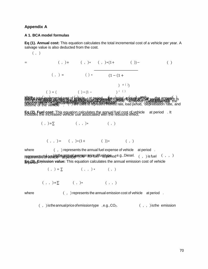
70

Appendix A

A 1. BCA model formulas

Eq (1). Annual cost: This equation calculates the total incremental cost of a vehicle per year. A salvage value is also deducted from the cost.

� � � � (� , � )

= � � � � � � � � � � � � � � (� , � ) + � � � � � (� , � ) ∗ � � � (� , � ) ∗ (1 + � � � � � � � (� )) − � � � � � � � � � � � (� )

� � � � � � � � � � � � � � (� , � ) = � � � � � � � � � � � (� ) ∗

� � � � � � � �

(1 − (1 +

� � � � � � � � )� � 𝑎� (� ))

� � � � � � � � � � � (� ) = (� � � � � � � � � � � (� ) ∗ (1 − � � � � � � � � � � � � )� 𝑖� � (� )

where � � � � (� , � ), � � � � � � � � � � � (� ), � � � � � � � � � � � � � � (� , � ), � � � � � (� , � ), and � � � � � � � � � � � (� ) are the total incremental cost of vehicle � at period � , the capital cost of vehicle � , the annual capital payments of vehicle � at period � , maintenance cost of vehicle � at period � , which is defined as dollar per km, and salvage cost of vehicle � when its life is over, respectively. � � � (� , � ) represents the vehicle kilometer traveled by vehicle � at period � , and based on the exponential decline formula defined earlier in the main text. � � � � � � � (� , � ) represents the rebound effect, i.e., annual increase rate of VKT, for vehicle � . � � � � � � � � , � � � � (� ), � � � � � � � � � � � � , and � � � � (� ) are used to represent interest rate, load period, depreciation rate, and lifetime of the vehicle � .

Eq (2). Fuel cost: This equation calculates the annual fuel cost of vehicle � at period � . It includes the increased vehicle use associated with the rebound effect.

� � � � � � � � (� , � ) = ∑ � � � � � � � � � � (� , � , � ) ∗ � � � � � � � � � (� , � )

�

� � � � � � � � � � (� , � , � ) = � � � (� , � ) ∗ (1 + � � � � � � � (� )) ∗ � � � � � � � (� , � )

where � � � � � � � � (� , � ) represents the annual fuel expense of vehicle � at period � .

� � � � � � � � � (� , � ) is the annual average price of fuel type, � , e.g., Diesel. � � � � � � � � � � (� , � , � ) represents the total demand of vehicle � for fuel � at period � . � � � � � � � (� , � ) is fuel � requirement of vehicle � at period � . Eq (3). Emission value: This equation calculates the annual emission cost of vehicle � at period � .

� � � � � � � � � � � � (� , � ) = ∑ � � � � � � � � � (� , � , � ) ∗ � � � � � � (� , � )

�

� � � � � � � � (� , � , � ) = ∑ � � � � � � (� , � ) ∗ � � � � � � � � � � (� , � , � )

�

where � � � � � � � � � � � � (� , � ) represents the annual emission cost of vehicle � at period � .

� � � � � � (� , � ) is the annual price of emission type � , e.g., CO2. � � � � � � � � � (� , � , � ) is the emission

71

level of emitter � from vehicle � at period � and � � � � � � (� , � ) is the quantity of emission type �

per unit of fuel � consumption at period � . Eq (4). Refilling cost: This equation calculates the cost spend for refilling the vehicle tank.

� � � � � � � � � � � � � (� , � ) � � � (� , � ) ∗ (1 + � � � � � � � (� )) ∗

� � � � � � � (� , � ) =

� � � � � � (� )

� � � � � � (� )

∗ (� � � � � � � � (� ) + � � � � � � � ) ∗ � � � � � � � � � � (� , � )

where � � � � � � � � � � � � � (� , � ) represents the cost of refilling the vehicle tank per hour. � � � � � � (� ) is the vehicle tank volume in liter, � � � � � � � � (� ) is the fuel dispense rate from fuel pump in a minute, e.g., liter per min, � � � � � � � is the fixed time spent per refill, and � � � � � � � � � � (� , � ) is the labor cost.

Eq (5). Rebound travel benefit: This equation calculates the benefits of increased vehicle use

associated with the rebound effect.

� � � � � � � � � � � � � (� , � ) = � � � (� , � ) ∗ � � � � � � � (� ) ∗ � � � � � � � � � � � � (� , � )

where � � � � � � � � � � � � � (� , � ) represents the economic benefits that become accessible with additional travel. � � � � � � � � � � � � (� , � ) is the profit of the company per unit distance traveled, e.g., dollar profit per km.

Eq (5). Energy security benefit: This equation defines the economic benefit of improvements in the India energy security.

� � � � � � � � � � � � � � 𝑇𝑃(� ) = (� � � � � � � � � � � 𝑎� � � 𝑖� � (� ) − � � � � � � � � � � 𝑇𝑃(� )) ∗ � � � _� � � � (� )

where � � � � � � � � � � � � � � 𝑇𝑃(� ) is the energy security premium, the avoided Indian macroeconomic disruption and adjustment cost, in period � and � � � _� � � � (� ) is the adjustment cost per unit of fuel reduction, e.g., dollar per liter fuel savings.

A 2. VKT decline by age with parameter α

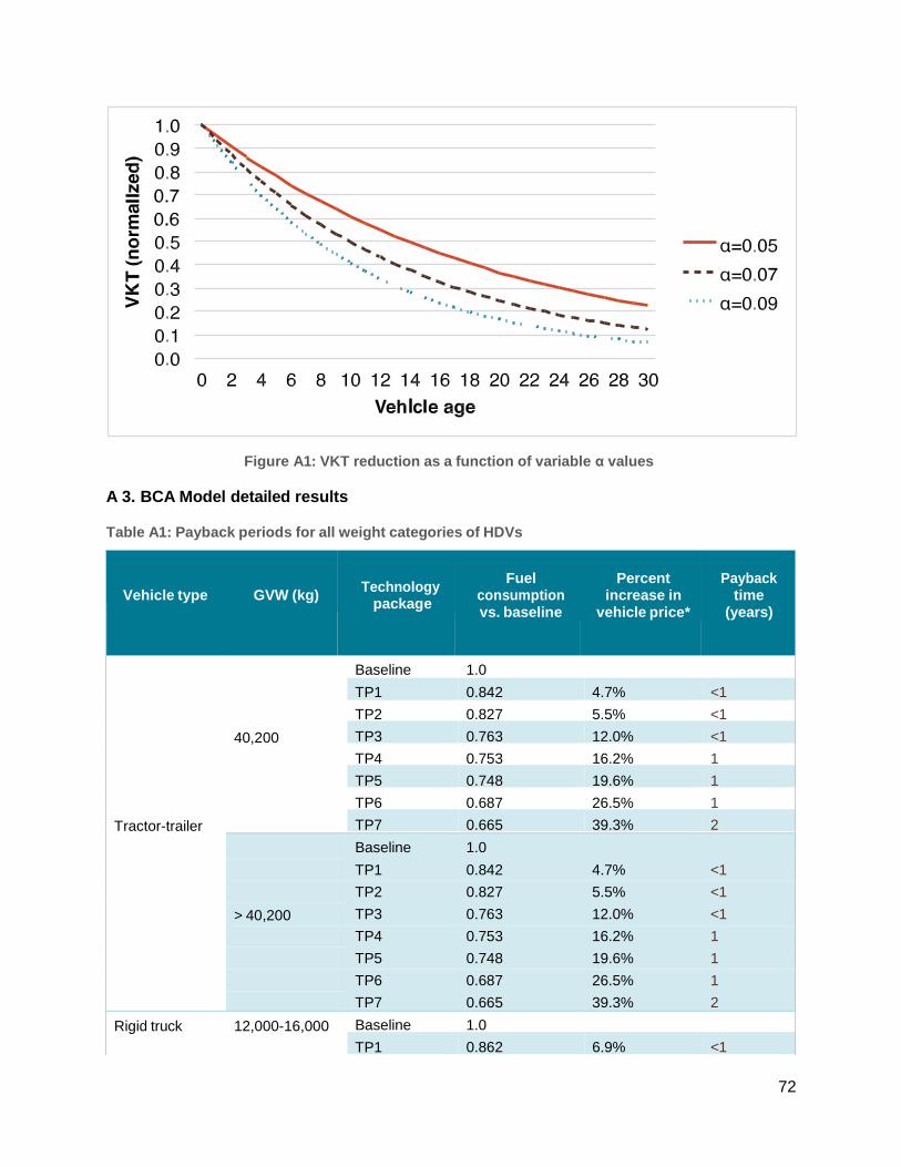
72

Figure A1: VKT reduction as a function of variable α values

A 3. BCA Model detailed results Table A1: Payback periods for all weight categories of HDVs

Vehicle type

GVW (kg)

Technology package

Fuel

consumption vs. baseline

Percent

increase in vehicle price*

Payback

time (years)

Tractor-trailer

Baseline 1.0

TP1 0.842 4.7% <1

TP2 0.827 5.5% <1

40,200 TP3 0.763 12.0% <1

TP4 0.753 16.2% 1

TP5 0.748 19.6% 1

TP6 0.687 26.5% 1

TP7 0.665 39.3% 2 Baseline 1.0

TP1 0.842 4.7% <1

TP2 0.827 5.5% <1

> 40,200 TP3 0.763 12.0% <1

TP4 0.753 16.2% 1

TP5 0.748 19.6% 1

TP6 0.687 26.5% 1

TP7 0.665 39.3% 2

Rigid truck 12,000-16,000 Baseline

TP1

1.0

0.862

6.9%

<1

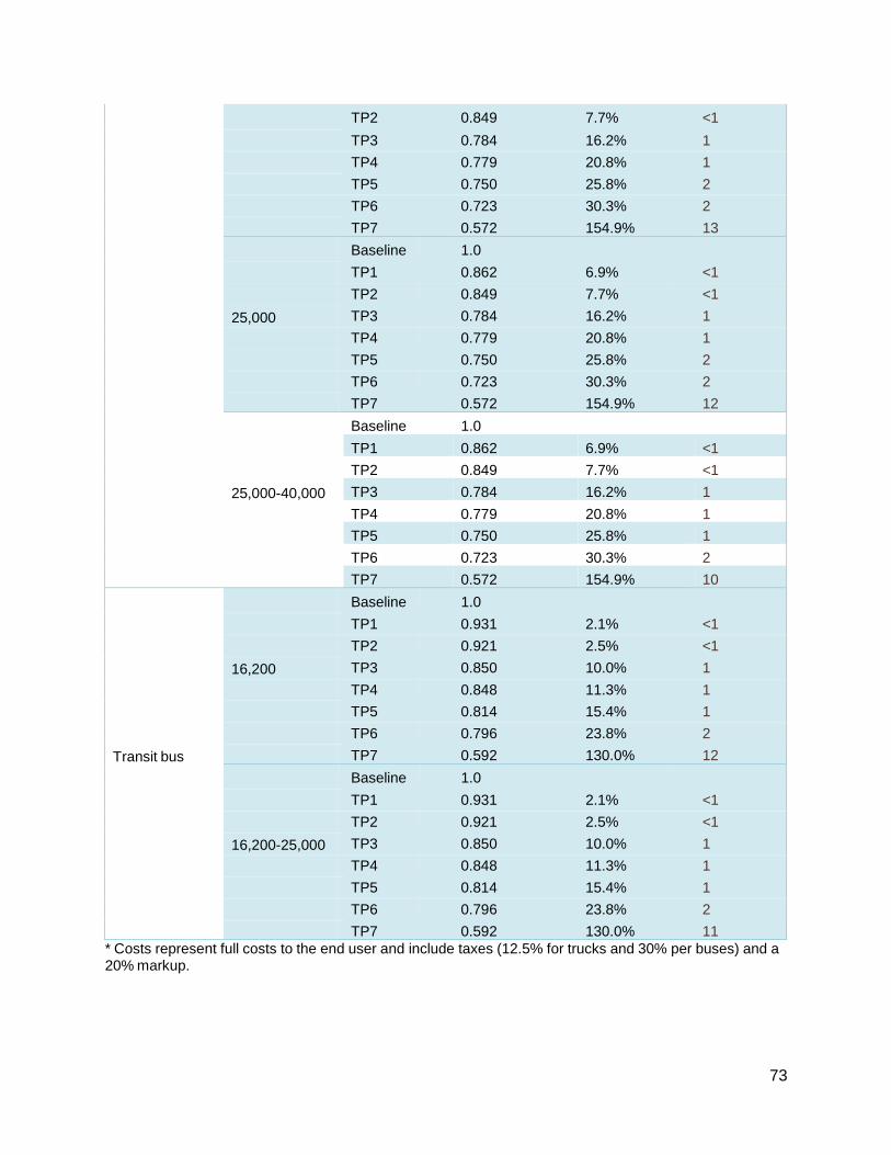
73

TP2 0.849 7.7% <1

TP3 0.784 16.2% 1

TP4 0.779 20.8% 1

TP5 0.750 25.8% 2

TP6 0.723 30.3% 2

TP7 0.572 154.9% 13 Baseline 1.0

TP1 0.862 6.9% <1

TP2 0.849 7.7% <1

25,000 TP3 0.784 16.2% 1

TP4 0.779 20.8% 1

TP5 0.750 25.8% 2

TP6 0.723 30.3% 2

TP7 0.572 154.9% 12 Baseline 1.0

TP1 0.862 6.9% <1

TP2 0.849 7.7% <1

25,000-40,000 TP3 0.784 16.2% 1

TP4 0.779 20.8% 1

TP5 0.750 25.8% 1

TP6 0.723 30.3% 2

TP7 0.572 154.9% 10

Transit bus

Baseline 1.0

TP1 0.931 2.1% <1

TP2 0.921 2.5% <1

16,200 TP3 0.850 10.0% 1

TP4 0.848 11.3% 1

TP5 0.814 15.4% 1

TP6 0.796 23.8% 2

TP7 0.592 130.0% 12 Baseline 1.0

TP1 0.931 2.1% <1

TP2 0.921 2.5% <1

16,200-25,000 TP3 0.850 10.0% 1

TP4 0.848 11.3% 1

TP5 0.814 15.4% 1

TP6 0.796 23.8% 2

TP7 0.592 130.0% 11 * Costs represent full costs to the end user and include taxes (12.5% for trucks and 30% per buses) and a 20% markup.

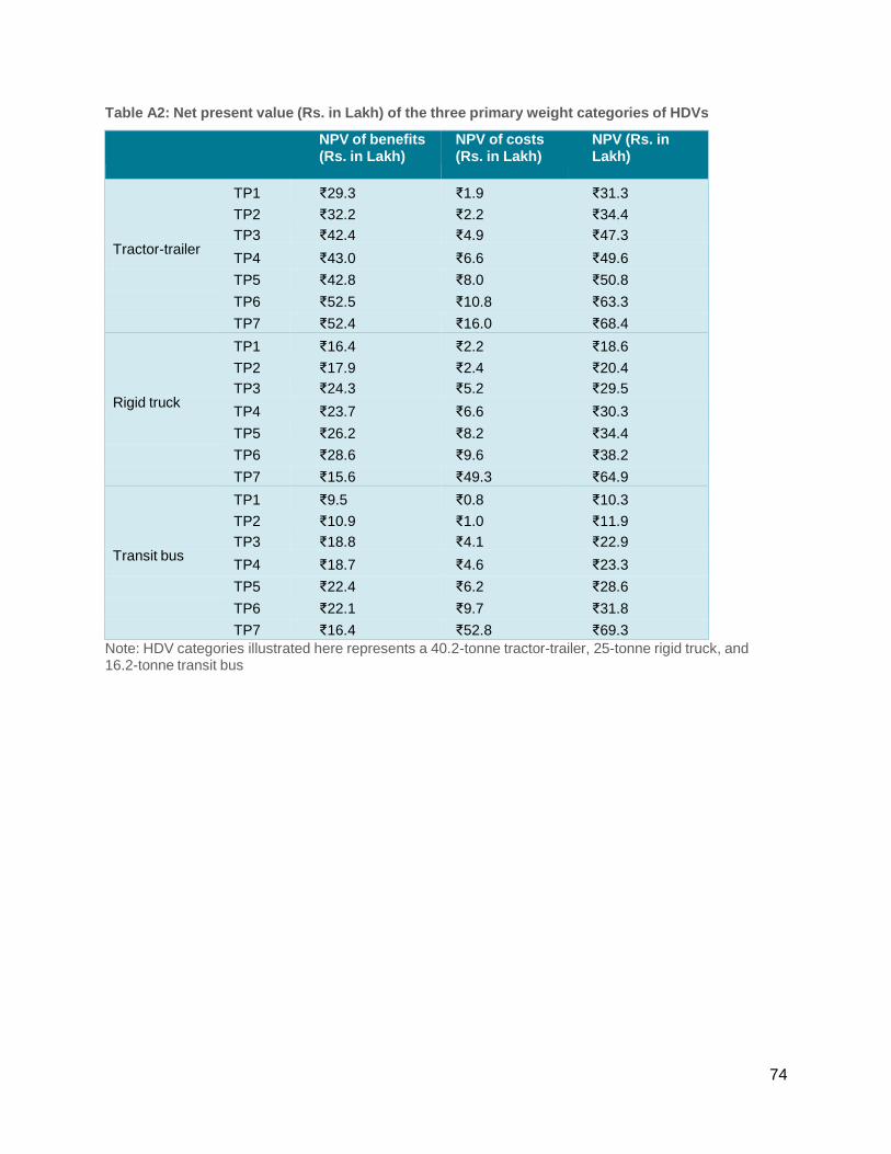
74

Table A2: Net present value (Rs. in Lakh) of the three primary weight categories of HDVs

NPV of benefits (Rs. in Lakh)

NPV of costs (Rs. in Lakh)

NPV (Rs. in Lakh)

TP1 ₹29.3 ₹1.9 ₹31.3

TP2 ₹32.2 ₹2.2 ₹34.4

TP3 ₹42.4 ₹4.9 ₹47.3 Tractor-trailer

TP4 ₹43.0 ₹6.6 ₹49.6

TP5 ₹42.8 ₹8.0 ₹50.8

TP6 ₹52.5 ₹10.8 ₹63.3

TP7 ₹52.4 ₹16.0 ₹68.4

TP1 ₹16.4 ₹2.2 ₹18.6

TP2 ₹17.9 ₹2.4 ₹20.4

TP3 ₹24.3 ₹5.2 ₹29.5 Rigid truck

TP4 ₹23.7 ₹6.6 ₹30.3

TP5 ₹26.2 ₹8.2 ₹34.4

TP6 ₹28.6 ₹9.6 ₹38.2

TP7 ₹15.6 ₹49.3 ₹64.9

TP1 ₹9.5 ₹0.8 ₹10.3

TP2 ₹10.9 ₹1.0 ₹11.9

TP3 ₹18.8 ₹4.1 ₹22.9 Transit bus

TP4 ₹18.7 ₹4.6 ₹23.3

TP5 ₹22.4 ₹6.2 ₹28.6

TP6 ₹22.1 ₹9.7 ₹31.8

TP7 ₹16.4 ₹52.8 ₹69.3 Note: HDV categories illustrated here represents a 40.2-tonne tractor-trailer, 25-tonne rigid truck, and 16.2-tonne transit bus

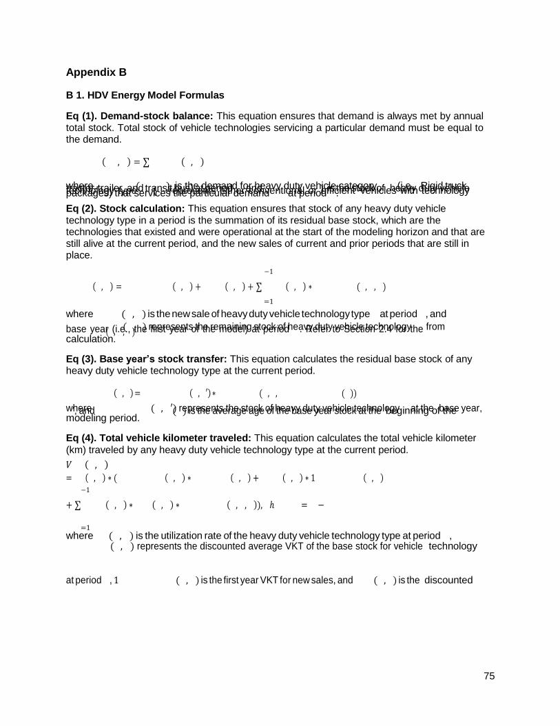
75

Appendix B

B 1. HDV Energy Model Formulas

Eq (1). Demand-stock balance: This equation ensures that demand is always met by annual total stock. Total stock of vehicle technologies servicing a particular demand must be equal to the demand.

� � � � � � (� � , � ) = ∑ � � � � � (� , � )

� where � � � � � � (� � , � ) is the demand for heavy duty vehicle category � � (i.e., Rigid truck, tractor-trailer, and transit bus) at period � , and � � � � � (� , � ) is the stock of heavy duty vehicle technology type � (� represents either conventional or efficient vehicles with technology packages) that services the particular demand � � at period � .

Eq (2). Stock calculation: This equation ensures that stock of any heavy duty vehicle technology type in a period is the summation of its residual base stock, which are the technologies that existed and were operational at the start of the modeling horizon and that are still alive at the current period, and the new sales of current and prior periods that are still in place.

� −1

� � � � � (� , � ) = � � � � � � � � � (� , � ) + � � � � (� , � ) + ∑ � � � � (� , � ) ∗ � � � � � � � � (� , � , � )

� =1

where � � � � (� , � ) is the new sale of heavy duty vehicle technology type � at period � , and

� � � � � � � � � (� , � ) represents the remaining stock of heavy duty vehicle technology � from base year (i.e., the first year of the model) at period � . Refer to Section 2.4 for the � � � � � � � � (� , � , � ) calculation.

Eq (3). Base year’s stock transfer: This equation calculates the residual base stock of any heavy duty vehicle technology type at the current period.

� � � � � � � � � (� , � ) = � � � � � � � � � (� , � ′) ∗ � � � � � � � � (� , � , � � � � � � � � � � � � (� ))

where � � � � � � � � � (� , � ′) represents the stock of heavy duty vehicle technology � at the base year, � ’, and � � � � � � � � � � � � (� ) is the average age of the base year stock at the beginning of the modeling period.

Eq (4). Total vehicle kilometer traveled: This equation calculates the total vehicle kilometer

(km) traveled by any heavy duty vehicle technology type at the current period.

𝑉� � (� , � )

= � � (� , � ) ∗ (� � � � � � � � � (� , � ) ∗ � � � � � � � (� , � ) + � � � � (� , � ) ∗ 1� � � � � � � � � (� , � ) � −1

+ ∑ � � � � (� , � ) ∗ � � � (� , � ) ∗ � � � � � � � � (� , � , � )), � ℎ� � � � = � − �

� =1 where � � (� , � ) is the utilization rate of the heavy duty vehicle technology type at period � , � � � � � � � (� , � ) represents the discounted average VKT of the base stock for vehicle technology �

at period � , 1� � � � � � � � � (� , � ) is the first year VKT for new sales, and � � � (� , � ) is the discounted

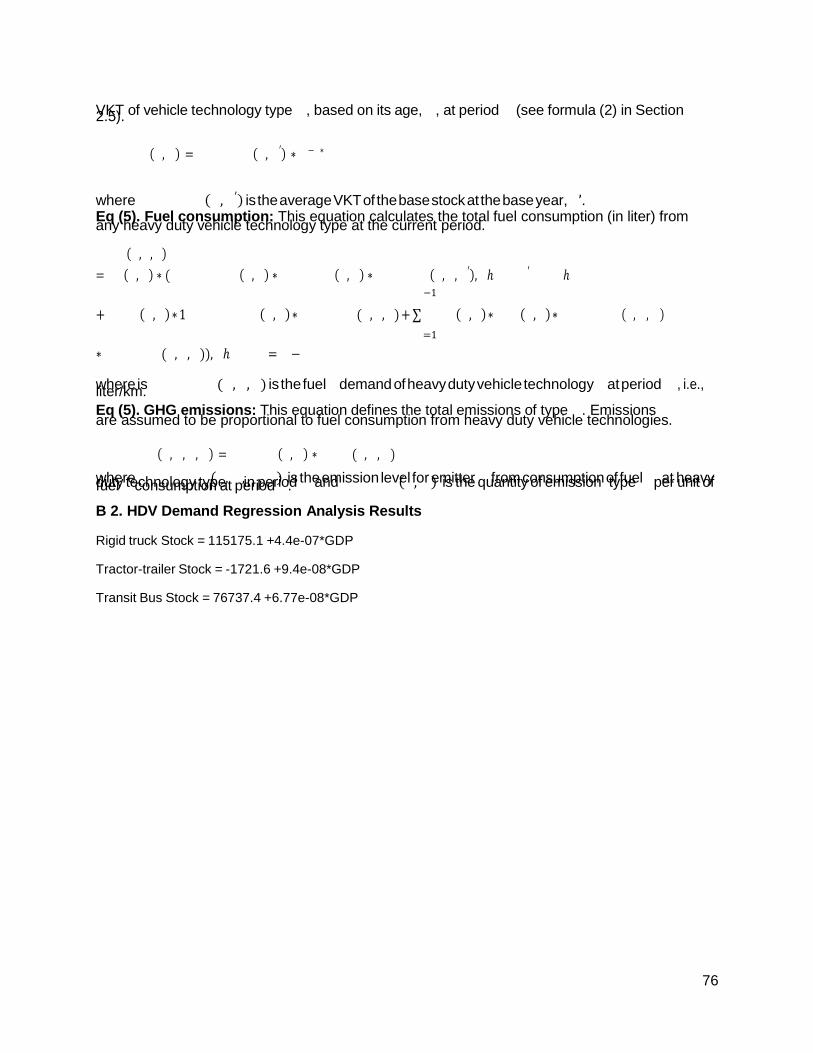
76

VKT of vehicle technology type � , based on its age, � , at period � (see formula (2) in Section 2.5).

� � � � � � � (� , � ) = � � � � � � � (� , � ′) ∗ � −� ∗�

where � � � � � � � (� , � ′) is the average VKT of the base stock at the base year, � ’. Eq (5). Fuel consumption: This equation calculates the total fuel consumption (in liter) from any heavy duty vehicle technology type at the current period.

� � � � (� , � , � )

= � � (� , � ) ∗ (� � � � � � � � � (� , � ) ∗ � � � � � � � (� , � ) ∗ � � � � � � � (� , � , � ′), � ℎ� � � � ′ � � � ℎ� � � � � � � � � � −1

+ � � � � (� , � ) ∗ 1� � � � � � � � � (� , � ) ∗ � � � � � � � (� , � , � ) + ∑ � � � � (� , � ) ∗ � � � (� , � ) ∗ � � � � � � � � (� , � , � )

� =1

∗ � � � � � � � (� , � , � )), � ℎ� � � � = � − �

where is � � � � � � � (� , � , � ) is the fuel � demand of heavy duty vehicle technology � at period � , i.e., liter/km.

Eq (5). GHG emissions: This equation defines the total emissions of type � . Emissions are assumed to be proportional to fuel consumption from heavy duty vehicle technologies.

� � � � � � � � (� , � , � , � ) = � � � � � � (� , � ) ∗ � � � � (� , � , � )

where � � � � � � � � (� , � , � , � ) is the emission level for emitter � from consumption of fuel � at heavy duty technology type � in period � and � � � � � � (� , � ) is the quantity of emission type � per unit of fuel � consumption at period � .

B 2. HDV Demand Regression Analysis Results

Rigid truck Stock = 115175.1 +4.4e-07*GDP

Tractor-trailer Stock = -1721.6 +9.4e-08*GDP

Transit Bus Stock = 76737.4 +6.77e-08*GDP

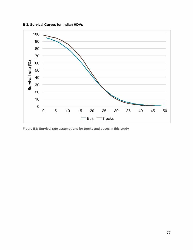
77

B 3. Survival Curves for Indian HDVs

Figure B1: Survival rate assumptions for trucks and buses in this study

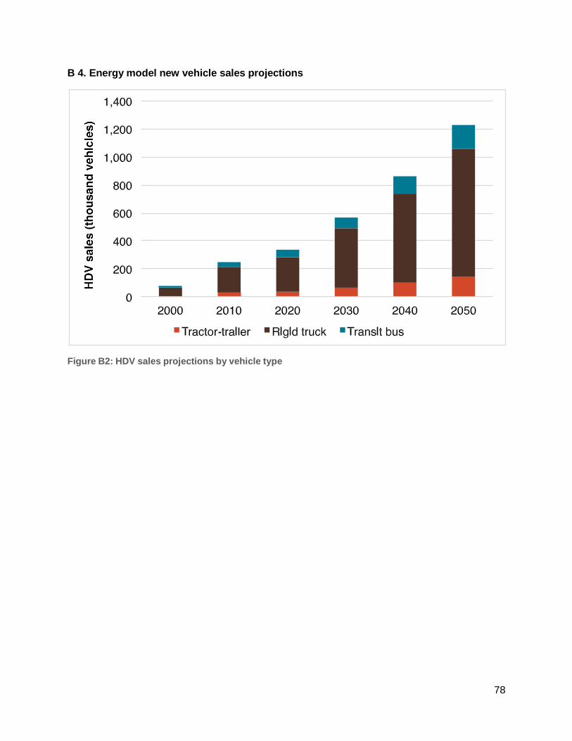
78

B 4. Energy model new vehicle sales projections

Figure B2: HDV sales projections by vehicle type

Documents

Improved heavy-duty vehicle fuel efficiency in India · Improved heavy-duty vehicle fuel efficiency in India Benefits, costs and environmental impacts Authors: ... Operational characteristics