Importance Sampled Learning Ensembles

Jerome H. Friedman∗ Bogdan E. Popescu†

September 9, 2003

Abstract

Learning a function of many arguments is viewed from the perspective of high–dimensional numerical quadrature. It is shown that many of the popular ensemblelearning procedures can be cast in this framework. In particular randomized methods,including bagging and random forests, are seen to correspond to random Monte Carlointegration methods each based on particular importance sampling strategies. Nonrandom boosting methods are seen to correspond to deterministic quasi Monte Carlointegration techniques. This view helps explain some of their properties and suggestsmodifications to them that can substantially improve their accuracy while dramaticallyimproving computational performance.

Keywords and phrases: learning ensembles, bagging, random forests, boosting, gra-dient boosting, AdaBoost, MART

1 Introduction

Approximating a function of many arguments is central to supervised learning problems indata mining, machine learning, and pattern recognition. The goal is to predict (estimate)likely values y for the unknown value y of a particular attribute (variable) associated with asystem under study, given the known joint values of other attributes x = (x1, x2, ···, xn) alsoassociated with that system. The prediction rule can be regarded as defining a functiony = F (x) that maps points x in the space χ of all joint values, x ∈χ, to values in thecorresponding space of y–values, (y, y) ∈ Y .

Defining a loss L(y, y) that characterizes the cost of predicting a value y when the truevalue is y, the lack of quality of the prediction rule is often taken to be the average orexpected loss (“risk”) over all future predictions

R(F ) = Eqt(z)L(y, F (x)) (1)

where z = (x, y) and qt(z) is is the joint distribution of future (“test”) attribute values. Inthis case the optimal “target” function is the one that minimizes prediction risk

F ∗(x) = arg minF (x)

Eqt(z)L(y, F (x)). (2)

∗Department of Statistics and Stanford Linear Accelerator Center, Stanford University, Stanford, CA94305 (jhf@stanford.edu)

†Department of Statistics, Stanford University, Stanford, CA 94305 (bogdan@stat.stanford.edu)

1

In the predictive learning problem one is given a collection of previously solved cases{zi = (xi, yi)}N

1 where for each individual case (observation) the values of all of the at-tributes have been observed. The prediction rule is constructed from this “learning” data

y = F (x) = F(x; {zi}N

1

).

The learning observations are often regarded as being a random sample drawn from someprobability distribution ql(z), where ql(z) ' qt(z) (1). Situations where ql(z) 6= qt(z) arereferred to as “concept drift” in the machine learning literature.

When ql(z) = qt(z) = q(z) the learning problem can be viewed as estimating F ∗(x) (2)given its approximate value

yi = F ∗(xi) + εi

at a set of randomly realized {xi}N1 . Here εi is a random variable with probability distri-

bution εi ∼ q(yi − F ∗(xi) |xi). The “distance” criterion to be minimized is

D(F, F ∗) = Eq(z) [L(y, F (x))− L(y, F ∗(x))] . (3)

2 Approximating Model

There are a great many methods proposed for predictive learning. (See for example, Hastie,Tibshirani, and Friedman 2001.) Here the focus in on linear prediction models of the form

F (x; a) = a0 +∫

Pa(p) f(x;p) dp, (4)

where f(x;p) (“base learner”) is a specified (often simple) function of the predicting vari-ables x, characterized by a set of parameters p = (p1, p2, · · ·pK). A specific set of jointparameter values p ∈P indexes a particular function of x from the set of all such functions{f(x;p)}p∈P , and a(p) is its corresponding coefficient in the linear model (4). Thus, givena particular base learner f(x;p), the coefficient function a(p) (along with the intercept pa-rameter a0) specifies the predicting model F (x; a). From (3) the optimal coefficient functionis given by

a∗ = arg mina

Eq(z)L(y, F (x; a)) (5)

and the corresponding function of x, F (x; a∗), is the optimal one for prediction among thosein the class of functions defined by the base learner through (4). If the target function F ∗(x)(2) resides in this class then F ∗(x) = F (x; a∗); otherwise F (x; a∗) represents the closestfunction to F ∗(x) in this class with distance defined by (3).

Popular base learners include sigmoids of linear combinations

f(x;p) =[1 + exp(ptx)

]−1 (6)

used in neural networks (Rumelhart, Hinton and Williams 1985), multivariate spline func-tions where the parameters are the knot locations on the respective variables (Friedman1991), and decision trees (Breiman, Friedman, Olshen and Stone 1981, Quinlan 1991) wherethe parameters are the splitting variables and values that define the partition of the pre-dictor variable space χ, and the values assigned to the terminal nodes.

2

3 Numerical quadrature

Computing F (x; a) (4) for any given x requires the evaluation of a multidimensional integralof the form ∫

PI(p) dp, (7)

where here the integrand is I(p) = a(p) f(x;p). It is unlikely that this integral can berepresented by an easily computable closed form. Thus numerical quadrature rules mustbe employed. Numerical quadrature approximates (7) by

∫

PI(p) dp '

M∑

m=1

wmI(pm) (8)

where I(pm) is the integrand evaluated at pm ∈ P , and wm is a corresponding weightapplied to the evaluation.

Specific quadrature rules are defined by choice of evaluation points {pm}M1 and corre-

sponding weights {wm}M1 . For (4) the quadrature rule becomes

F (x; a) ' a0 +M∑

m=1

wm a(pm) f(x;pm) = F(x; {cm}M

0

)= c0 +

M∑

m=1

cm f(x;pm) (9)

with c0 = a0 and cm = wm a(pm), since wm and a(pm) are not separately identifiable. Fora given set of evaluation points {pm}M

1 the optimal coefficient values, averaged over all xvalues, are (from (3)) given by

{c∗m}M0 = arg min

{cm}M0

Eq(z)L(y, F

(x; {cm}M

0

)). (10)

Thus, knowing the joint distribution q(z), the problem becomes one of choosing a good setof evaluation points {pm}M

1 for constructing the approximating quadrature rule (9). Ofcourse q(z) is not known; only a random sample {zi}N

1 drawn from this distribution is avail-able. This complication is addressed in Section 5. For now we only consider the idealized(computational) problem of choosing a good quadrature rule given the joint distributionq(z).

4 Monte Carlo methods

Most useful base learners f(x;p) (4) involve several to many parameters. Thus, the in-tegration problem (7) is high dimensional. Among the most successful high dimensionalquadrature rules are those based on Monte Carlo methods. The set of evaluation points{pm}M

1 are randomly drawn from some probability distribution r(p) defined on the param-eter space p ∈ P . This distribution defines the Monte Carlo integration rule. The simplestrule chooses r(p) to be constant so that any point p ∈ P is equally likely to be selected ateach of the M draws. Other choices for r(p) define alternative Monte Carlo rules; the bestchoice as judged by (3) will depend on the target function F ∗(x) (2).

3

4.1 Importance sampling

The goal of importance sampling Monte Carlo is to increase accuracy by using informationknown about a particular problem to choose a good sampling probability distribution r(p)for that problem. The cardinality M of the selected points is generally a small fractionof all p ∈ P so that judicious choices for {pm}M

1 can often dramatically increase accuracyover simple constant probability sampling. The challenge is to identify what informationis known, or easily obtained, about the problem at hand and then using it to constructan appropriate sampling distribution r(p). To be effective, this distribution should assignrelatively high mass to points in the parameter space p ∈ P that are more relevant orimportant to achieving a high accuracy integration rule when used with a relatively smallnumber of other evaluation points, and with the coefficients (weights) given by (10).

In general, the incremental value of any selected point pm for reducing approximationerror (3) will depend on the other points included with it in the quadrature rule. Therefore,importance values should be assigned to groups of points taken together as being propor-tional to the accuracy of the rule based on those points. Unfortunately, even approximatelydetermining such group importances, for all possible groupings, is very difficult to do inpractice for any given problem. Approximate sequential sampling strategies, based on es-timating the importance of a single point pm conditional on the previously selected points{pm′}m′<m can sometimes be employed. This is discussed in Section 7.

We begin by considering the simplest importance sampling strategies for which theimportance or relevance of an evaluation point pm is estimated without regard to the otherpoints that might be used with it in the integration rule. As discussed in Section 6, thisis the strategy used by bagging (Breiman 1996a), random forests (Ho 1995 and Breiman2001), and Bayesian model averaging (Denison, Holmes, Mallik and Smith 2002, Chipman,George and McCullagh 1998). Although less than ideal, such strategies can often result indramatic gains in accuracy over naive constant probability sampling.

4.2 Partial importance

Given only a single potential evaluation point p ∈ P , without knowledge of the other pointsthat will be used with it in the integration rule, one measure of its lack of relevance is

J(p) = minα0,α

Eq(z)L(y, α0 + α f(x,p)). (11)

This is the prediction risk of using p alone in a single point (M = 1) rule (9). The optimalsingle point rule is obtained by using

p∗ = arg minp∈P

J(p). (12)

Although this optimal single point rule is unlikely to be as accurate as one involving manyevaluation points, it is commonly used in practice. This is the case, for example, when asingle decision tree or logistic regression is employed.

This measure (11) is clearly an imperfect reflection of the (inverse) value of a point whenit is used together with other points in a quadrature rule. It is possible for a particularpoint p to have a small value of J(p) but still contribute little toward increasing accuracyin the presence of a given set of other evaluation points. Although perhaps less likely, itis also possible for J(p) to be relatively large for evaluation points that can significantly

4

aid in increasing accuracy when used in conjunction with particular sets of other points.However, (11) represents an easily computable importance surrogate. The assumption(hope) is that a collection of such evaluation points {pm}M

1 , each with relatively smallvalues of J(pm), will result in a integration rule with higher accuracy than with either asimilar sized collection of points sampled with constant probability, or the best single pointrule (12). As evidenced by the success of bagging and random forests, this is often the casein practice.

4.3 Partial importance sampling

In order to apply importance sampling Monte Carlo based on J(p) (11), one must derivea sampling probability density r(p) that gives higher probability to points p ∈ P withsmaller values of J(p). That is

r(p) = g(J(p)) (13)

with g(·) a monotonically decreasing function of its argument. This density will be centeredat or near p∗ (12) and have correspondingly decreasing values for points p increasinglydistant from p∗. Here the relevant distance measure is

d(p,p∗) =J(p)− J(p∗). (14)

In addition to its location, it is well known that a critical parameter of any probabilitydensity used for importance sampling is its characteristic scale

σ =∫

Pd(p,p∗) r(p) dp. (15)

If σ is too large then too few points of high importance will be sampled, thereby decreasingthe accuracy of the resulting integration rule. In the extreme limit of very large values of σthe result will be similar to that of naive constant probability Monte Carlo. If the value ofσ is too small then each sampled point provides little additional information beyond thatprovided by the other nearby sampled points used with it. In the extreme limit of σ = 0,r(p) = δ(p − p∗), where δ(·) is the Dirac delta function. In this case the integration rulewill have the same accuracy as that of the best single point (M = 1) rule (12) regardless ofthe number of sampled points actually used. In any particular problem there is an unknownoptimal value for σ. It will depend on M and the detailed nature of the problem at hand,namely the joint distribution of the attributes q(z) and the choice of base learner f(x;p).

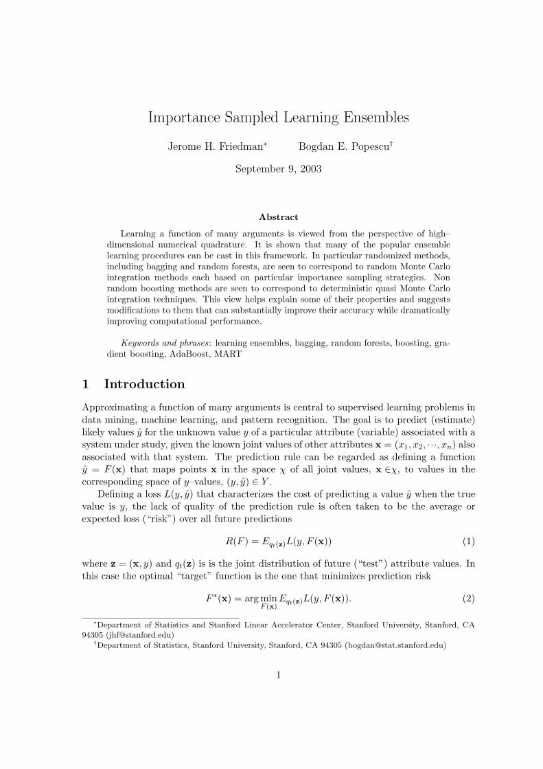
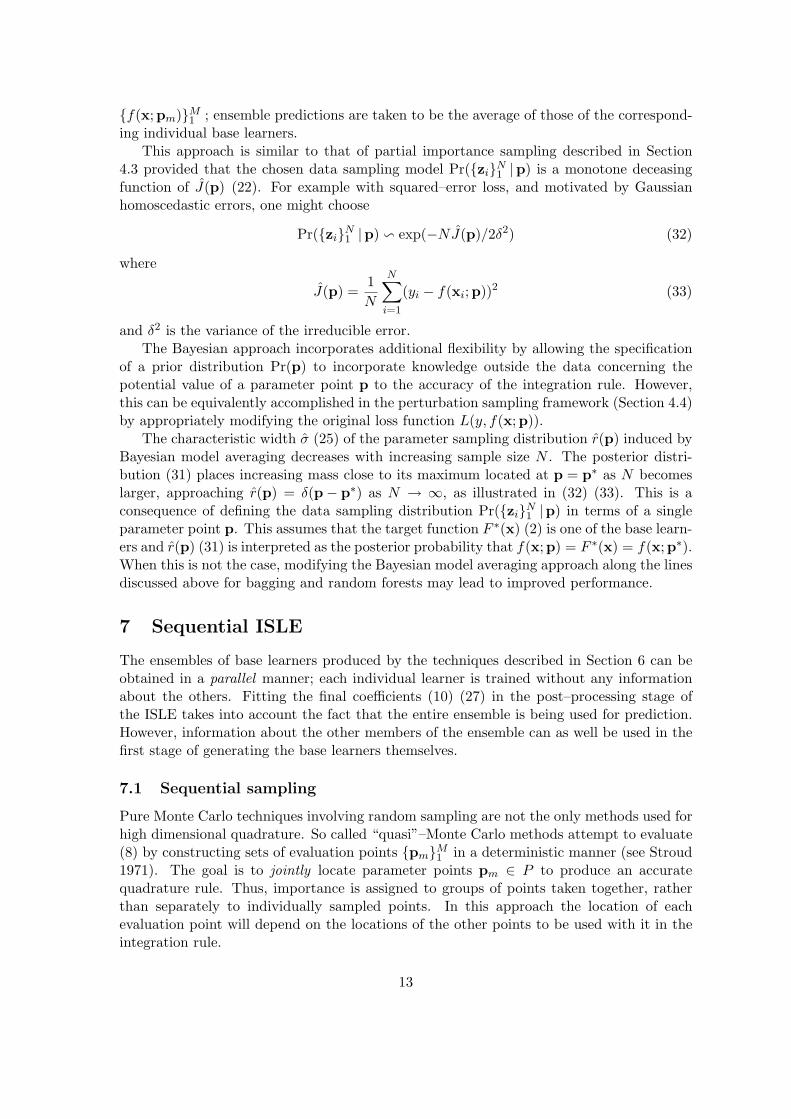
These concepts are illustrated in the context of simple importance sampling Monte Carlointegration in Fig. 1. The upper (black) curve represents a function F (p) to be integratedover the real line −∞ < p < ∞, and the lower (colored) curves represent several potentialsampling distributions r(p). Each distribution is characterized by a respective location andscale. The almost constant (lower orange) curve is located near the maximum of F (p) buthas a very large scale thereby placing only a small fraction of sampled points where theintegrand is large (important). The (blue) curve to the right has the proper scale but isnot located near the important region of F (p), thereby also producing a small fraction ofimportant evaluation points. The narrow (red) distribution is centered near the maximumof F (p) and produces all of its evaluation points where F (p) is large. However, its small scalecauses very few points to be sampled in other regions where F (p) also assumes substantial

5

−1.0 −0.5 0.0 0.5 1.0

05

1015

2025

Figure 1: Various importance sampling distributions (lower colored curves) for integratingthe function represented by the upper (black) curve. The (blue) curve with location andscale similar to that of the integrand represents the most efficient among these importancesampling distributions.

values, thereby leading to an inaccurate result. The broader (green) distribution has boththe proper location and scale for integrating F (p) by covering the entire region where F (p)assumes substantial values while producing relatively few points in other regions. It therebyrepresents the most efficient sampling distribution for this particular problem.

Although very simple, the example shown in Fig. 1 illustrates the concepts relevant toimportant sampling Monte Carlo. Both the location and scale of the parameter samplingdistribution r(p) must be chosen appropriately so as to place most of its mass in all regionswhere the integrand realizes important values, and relatively small mass elsewhere. Forpartial importance sampling (11) (13) the parameter sampling distribution r(p) is locatednear the optimal single point rule p∗ (12). Its scale σ (15) is determined by the choice ofg(·) (13) which in turn is controlled by the details of the sampling strategy as discussedbelow.

Choosing the width (15) of r(p) is related to the empirically observed trade-off be-tween the “strength” of the individual learners and the correlations among them (Breiman2001). The strength of a base learner f(x,p) is directly related to its partial importance(inversely related to its lack of importance J(p) (11)). An ensemble of strong base learners{f(x,pm)}M

1 , all of which have J(pm) ' J(p∗) is well known to perform poorly, as doesan ensemble consisting of all very weak learners J(pm) À J(p∗). Best results are obtainedwith ensembles of moderately strong base learners whose predictions are not very highlycorrelated with each other.

A narrow sampling distribution (small σ (15)), produces base learners {f(x,pm)}M1 all

of which having similar strength to the strongest one f(x,p∗) (12), and thereby yieldingsimilar highly correlated predictions. This is analogous to the narrow (red) curve in Fig. 1.

6

A very broad r(p) (large σ) produces highly diverse base learners, most of which have largervalues of J(p) (smaller strength) and less correlated predictions. This corresponds to thealmost constant lower (orange) curve in Fig. 1. Thus, finding a good strength-correlationtrade-off for a learning ensemble can be understood in terms of seeking an appropriatewidth for an importance sampling parameter distribution (13) (15). As seen above, thebest width and thus best strength-correlation trade-off point, will depend on the particularproblem at hand as characterized by its true underlying target function F (x∗) (2).

4.4 Perturbation sampling

For any given problem finding, and then sampling from, an appropriate density r(p) onthe parameter space p ∈ P is usually quite difficult. However, there is a simple trick thatcan indirectly approximate this process. The idea is to repeatedly modify or perturb in arandom way some aspect of the problem, and then find the optimal single point rule (12) foreach of the modified problems. The collection of these single point solutions is then usedfor the quadrature rule. The characteristic width σ (15) of the corresponding samplingdistribution r(p) is controlled by the size of the perturbations. Aspects of the problem thatcan be modified are the loss criterion L(y, y), the joint distribution of the variables q(z),and the specifics of the algorithm used to solve the optimization problem (12).

For example, one could repeatedly perturb the loss criterion by

Lm(y, y) = L(y, y) + η · lm(y, y) (16)

where each lm(y, y) is a different randomly constructed function of its arguments. Thesampled points are obtained by

{pm = arg min

α0,α,p∈PEq(z)Lm(y, α0 + αf(x;p))

}M

1

. (17)

Alternately, one could repeatedly modify the argument to the loss function in a randomway, for example taking

{pm = arg min

α0,α,p∈PEq(z)L(y, α0 + αf(x;p) + ηgm(x))

}M

1

. (18)

Here each gm(x) is a different randomly constructed function of x. In both cases, theexpected size of the perturbations is controlled by the value of η which thereby indirectlycontrols the width σ of the corresponding sampling distribution r(p).

Another approach is to repeatedly modify the joint distribution of the variables byrandom reweighting

qm(z) = q(z) · [wm(z)]η (19)

where each wm(z) is a different randomly constructed (weighting) function of z. Thecollection of sampled points {pm}M

1 are the respective solutions to{pm = arg min

α0,α,p∈PEqm(z)L(y, α0 + αf(x;p))

}M

1

. (20)

Again the width σ of the corresponding sampling distribution r(p) is controlled by thevalue chosen for η.

7

Another method for perturbation sampling involves directly modifying in a random wayvarious aspects of the algorithm used to solve (12). The collection of outputs {pm}M

1 fromeach of these randomly perturbed algorithms is then used in the quadrature rule (9) (10).Most algorithms for solving (12) iteratively perform repeated partial optimizations oversubsets of the parameters as they converge to a solution. At each iteration the solutionvalues for each of these internal partial optimizations are replaced by alternative randomlychosen values. The degree to which these alternative values are constrained to be close totheir corresponding optimal solution values (indirectly) controls the width σ of the samplingdistribution r(p). For example, Dietterich 2000 replaces the optimal split at each recursivestep of decision tree construction by a random selection among the k best splits. Here thevalue chosen for k controls the width σ. Breiman 2001 chooses the optimal split among arandomly chosen subset of the predictor variables. The size of this subset inversely controlsthe degree of the perturbations, thereby regulating the width of r(p).

The implicit goal of all of these perturbation techniques is to produce a good set ofparameter points p ∈ P to be used with a quadrature rule (9) (10) for approximatingthe optimal predictor F (x; a∗) (4) (5). Their guiding principle is the notion of partialimportance sampling (11) (13), which produces a parameter sampling distribution r(p)that puts higher mass on points p that tend to have smaller risk when used in a MonteCarlo integration rule to evaluate (9). A critical meta–parameter of such procedures isthe characteristic width σ (15) of the indirectly induced sampling distribution r(p). Thisaspect is discussed in detail below.

5 Finite data

The discussion so far has presumed that the joint distribution q(z) of the variables z = (x, y)is known, and the expected values in (10) (11) can be calculated. As noted in Section 1,this is not the case in practice. Instead one has a collection of previously solved cases {zi}N

1

drawn from that distribution representing an empirical point mass approximation

q(z) =1N

N∑

i=1

δ(z− zi). (21)

This must serve as a surrogate for the unknown population distribution q(z). Becauseq(z) 6= q(z), complications emerge when the goal is to approximate the target functionF ∗(x) (2) by F (x, a∗) (4) (5), since both are based on the population distribution q(z).

5.1 Sampling

One such complication involves the sampling procedure. The partial importance J(p) (11)of a parameter point p ∈ P is unknown and must be approximated by

J(p) = minα0,α

Eq(z)L(y, α0 + αf(x;p)) (22)

with the corresponding optimal single point rule (12) approximated by

p = arg minp∈P

J(p). (23)

8

Equivalently, perturbation sampling (Section 4.4) must be based on the empirical distri-bution q(z) (21) rather than q(z), yielding an empirical parameter sampling distributionr(p).

Implementation of perturbation sampling (Section 4.4) on the data distribution (21) isstraight forward. The strategies corresponding to randomizing the loss criterion or randomalgorithm modification are unaltered. One simply substitutes q(z) for q(z) respectively in(17), (18), or the distribution to which an randomized algorithm is applied. Modificationof the joint distribution (19) can be accomplished by randomly weighting the observations

qm(z) =N∑

i=1

wim · δ(z− zi) (24)

where {wim}Ni=1 are randomly drawn from some probability distribution with E(wim) =

1/N . For a given sample size N , the scale (coefficient of variation) of the weight distributioncontrols the characteristic width σ (25) of the parameter sampling distribution r(p).

To the extent that the parameter estimates p (23) approach their corresponding popu-lation values p∗ (12) as the sample size N increases, the characteristic width

σ =∫

P[J(p)− J(p)] r(p)dp (25)

of r(p) will become smaller with increasing N for a given coefficient of variation of theweights. Therefore as N → ∞, r(p) → δ(p − p∗), and the Monte Carlo integration rulereduces to that of the optimal single point (M = 1) rule. As noted in Section 4.3, this isunlikely to produce the best results except in the unlikely event that the target functionF ∗(x) (2) is a member of the set of base learners; that is F ∗(x) = f(x;p∗). This suggeststhat the coefficient of variation of the weights should increase with increasing sample sizein order to maintain the width σ of the corresponding parameter sampling distribution r(p).

From a computational perspective, the most efficient random weighting strategy (24) isto restrict the weight values to wim ∈ {0, 1/K}, where K ≤ N is the number of non–zeroweight values. This can be accomplished by randomly selecting K observations, withoutreplacement from the collection of all N observations, to have non–zero weights. Thecoefficient of variation of all weight values is

C({wim}Ni=1) = (N/K − 1)1/2, (26)

so that, for a given sample of size N , reducing K increases the characteristic σ of r(p)while also reducing computation by a factor of K/N . Also, as discussed in the precedingparagraph, the value of K should grow more slowly than linearly with increasing N in orderto maintain the width σ of the corresponding parameter sampling distribution r(p).

5.2 Quadrature coefficients

A second problem caused by finite data is determining the quadrature coefficients {cm}M0

(9) given a set of evaluation points {pm}M1 . The optimal coefficient values are given by

(10). These are based on the unknown population distribution q(z) and therefore must beestimated by using the empirical distribution q(z) (21). This is a standard linear regression

9

problem where y is the response (outcome) variable and the “predictors” are the baselearners {f(x;pm)}M

1 corresponding to the selected parameter evaluation points.There are a wide variety of linear regression procedures, many of which take the form

{cm}M0 = arg min

{cm}M0

1N

N∑

i=1

L

(yi, c0 +

M∑

m=1

cmf(xi;pm)

)+ λ ·

M∑

m=1

h(| cm − c(0)m |). (27)

The first term in (27) is the empirical risk on the learning data obtained by simply sub-stituting q(z) (21) for q(z) in (10). By including the second “regularization” term, oneattempts to increase accuracy through reduced variance of the estimated coefficient valuesby “shrinking” them towards a prespecified set of values {c(0)

m }M1 . This is accomplished by

choosing the function h(·) to be a monotone increasing function of its argument; usually

h(u) = uγ , γ ≥ 0. (28)

Popular choices for the value of γ are γ = 2 (“ridge regression”, Hoerl and Kannard 1971),and γ = 1 (“ShureShrink”, Donoho and Johnstone 1996 and “Lasso”, Tibshirani 1996). Theamount of shrinkage is regulated by λ ≥ 0 which is a model selection “meta” parameter ofthe regression procedure. Its value is chosen to minimize estimated future prediction risk.The most popular choice for the shrinkage targets is {c(0)

m = 0}M1 , reflecting prior lack of

knowledge concerning the signs of the population coefficient values {c∗m}M1 (10).

In the present application, the shrinkage implicit in (27) has the important functionof reducing bias of the coefficient estimates as well as variance. The importance samplingprocedure selects predictors f(x;pm) that have low empirical risk J(p) (22) and therebypreferentially high values for their empirical partial regression coefficients

αm = arg minα0,α

Eq(z)L(y, α0 + αf(x;pm)). (29)

If the multiple regression coefficients {cm}M1 were estimated using data independent of that

used to select {pm}M1 , then using (27) with λ = 0 would produce unbiased estimates.

However, using the same data for selection and estimation produces coefficient estimatesthat are biased towards high absolute values (see Copas 1983). The shrinkage provided by(27) for λ > 0 helps compensate for this bias.

The value chosen for the exponent γ in the penalty function (28) reflects one’s prior beliefconcerning the relative values of {| c∗m−c

(0)m |}M

1 . Higher values for γ produce more accurateestimates to the extent these absolute differences have equal values. For {c(0)

m = 0}M1 , this

implies that all of the f(x;pm) are equally relevant predictors. When this is not the case,smaller values of γ will give rise to higher accuracy. In the context of partial importancesampling (Section 4.3), the dispersion of importances among the respective f(x;pm) isroughly controlled by the characteristic width σ (25) of the empirical parameter samplingdistribution r(p). Thus, there is a connection between choice of regularizer h(u) in (27)and the sampling strategy used to select the predictors {f(x;pm)}M

1 .

6 ISLE

The previous sections outline in general terms the ingredients comprising an importancesampled learning ensemble (ISLE). They consist of an importance sampling strategy (Sec-tion 4.3), implemented by perturbation sampling (Section 4.4), on the empirical data dis-tribution (Section 5.1) to select a set of parameter evaluation points {pm}M

1 for a numerical

10

integration quadrature rule. The corresponding coefficients (weights) {cm}M1 assigned to

each of the evaluation points are calculated by a regularized linear regression (27) using thecorresponding selected base learners {f(x;pm)}M

1 as predictor variables. In this section weshow how several popular ensemble learning methods can be cast within this framework.This in turn helps explain some of their properties and suggests improvements to them thatcan (often dramatically) increase both their statistical and especially their computationalproperties.

6.1 Bagging

Bagging (Breiman 1996a) is an elegantly simple ensemble learning method. Each member ofthe learning ensemble is obtained by fitting the base learner to a different booststrap sample(Efron and Tibshirani 1993) drawn from the data. Ensemble predictions are taken to bethe average of those of the individually fitted base learners. In many applications baggedensembles achieve considerably lower prediction risk than the single estimated optimal baselearner (23). This is especially the case when the base learners are decision trees (Breimanet al 1983, Quinlan 1992).

The learning ensemble produced by bagging is clearly an ISLE. The parameter eval-uation points {pm}M

1 are obtained by (20), substituting (24) for qm(z) with the weights{wim}N

i=1 independently drawn from a multinomial distribution wim ∈ {0, 1, · · ·, N} withprobability 1/N . The quadrature coefficients are obtained from (27) with {c(0)

m = 1/M}M1

and λ = ∞, thereby reducing the quadrature rule (9) to being a simple average.When viewed form this perspective some of the properties of bagged ensembles are

easily understood. As with any ISLE, one should not expect substantial gains in accuracyfor base learners that are linear in the parameters

f(x,p) = p0 +∑

pjxj ,

since from (4) the ensemble spans the same space of functions as does the base learner, andthus does not enlarge that space.

It is also apparent that for any base learner f(x;p), the learning capacity of a baggedensemble does not increase with its size M . This is a consequence of using λ = ∞ in (27).The quadrature regression coefficients are set to prespecified constants rather than beingfit to the data. Thus bagging does not “over fit” the data when M is arbitrarily increased.In fact, the learning capacity of a bagged ensemble is generally less than that of the singlebest base learner (23) since the individual ensemble members (20) are optimized on qm(z)(24) rather than q(z) (21).

Viewing bagging as an ISLE suggests several straight forward modifications that mightimprove its performance. First, the use of bootstrap sampling induces a particular expectedlevel of perturbation on the learning sample. The expected coefficient of variation of thebootstrap observation weights is

E CB({wim}Ni=1) = (1− 1/N)1/2. (30)

Comparing this with (26), one sees that bagging with bootstrap samples is roughly equiv-alent to half–sampling without replacement. This in turn indirectly specifies a particularcharacteristic width σ (25) of the parameter sampling distribution r(p). As discussed inSection 5.1, this width will decrease with increasing sample size N . It is not clear that the

11

particular width induced by bagging is optimal for any given situation. Other perturbationstrategies that induce different characteristic widths might perform better. Second, thetotal regularization implied by λ = ∞ in (27) may not be optimal. Setting λ < ∞ andthereby allowing some level of coefficient fitting to the data may improve performance.

6.2 Random forests

Random forests (Breiman 2001) represents a hybrid approach involving random modifica-tions to both the joint distribution qm(z) (24) and the algorithm used to solve (22) (23).The base learners f(x,p) are taken to be decision trees grown to largest possible size withno pruning. As with bagging, each member of the learning ensemble is obtained by con-structing such a tree on a different bootstrap sample drawn from the data. In addition, ateach successive split during tree construction the optimal splitting variable is chosen from arandomly chosen subset of the predictor variables rather than from all of them. Ensemblepredictions are taken to be the average of those over all of the individual trees.

Including the random splitting has the effect of increasing the characteristic width σ(25) of the parameter sampling distribution r(p) beyond that obtained by using baggingalone. Here the parameters are the identities of the splitting variables and the splittingvalues. The degree of increase in σ is inversely controlled by the size ns of the selectedvariable subset at each split. Breiman 1998 suggests choosing ns = blog2(n) + 1c, wheren is the total number of predictor variables. Subset splitting has the additional effect ofreducing computation by a factor of ns/n.

Like a bagged ensemble, a random forest is clearly an ISLE sharing the same basicproperties discussed in Section 6.1. In particular, its learning capacity (less than baggedtrees of the same size) does not increase with its size M (number of trees). Its distinguishingcharacteristic is a broader parameter sampling distribution r(p) controlled by the numberof variables ns used to determine each split. Since the optimal width σ (25) is problemdependent, the relative accuracy of the two approaches will depend on the problem at hand.Also, random forests are amenable to the same potential improvements discussed in the lastparagraph of Section 6.1. In addition to adjusting ns, one can as well control σ by alteringthe data sampling strategy. Also setting λ < ∞ in (27), allowing the tree weights to be(partially) fit to the data, may improve performance.

6.3 Bayesian model averaging

Bayesian methods produce a parameter sampling distribution r(p) by proposing a samplingmodel Pr({zi}N

1 |p) for the data {zi}N1 given a parameter evaluation point p, and a prior

distribution Pr(p) for the parameters p ∈ P . The parameter sampling distribution is takento be the corresponding posterior distribution of p given the data

r(p) = Pr(p | {zi}N1 ) =

Pr({zi}N1 |p) Pr(p)∫

P Pr({zi}N1 |p) Pr(p) dp

. (31)

The sampled points {pm}M1 are intended to be independent draws from this distribution.

In practice this is approximated by Markov chain Monte Carlo methods which use a se-quence of dependent draws that converge to a stationary distribution identical to r(p) (31).The realized set of parameter points produce a corresponding ensemble of base learners

12

{f(x;pm)}M1 ; ensemble predictions are taken to be the average of those of the correspond-

ing individual base learners.This approach is similar to that of partial importance sampling described in Section

4.3 provided that the chosen data sampling model Pr({zi}N1 |p) is a monotone deceasing

function of J(p) (22). For example with squared–error loss, and motivated by Gaussianhomoscedastic errors, one might choose

Pr({zi}N1 |p) v exp(−NJ(p)/2δ2) (32)

where

J(p) =1N

N∑

i=1

(yi − f(xi;p))2 (33)

and δ2 is the variance of the irreducible error.The Bayesian approach incorporates additional flexibility by allowing the specification

of a prior distribution Pr(p) to incorporate knowledge outside the data concerning thepotential value of a parameter point p to the accuracy of the integration rule. However,this can be equivalently accomplished in the perturbation sampling framework (Section 4.4)by appropriately modifying the original loss function L(y, f(x;p)).

The characteristic width σ (25) of the parameter sampling distribution r(p) induced byBayesian model averaging decreases with increasing sample size N . The posterior distri-bution (31) places increasing mass close to its maximum located at p = p∗ as N becomeslarger, approaching r(p) = δ(p− p∗) as N → ∞, as illustrated in (32) (33). This is aconsequence of defining the data sampling distribution Pr({zi}N

1 |p) in terms of a singleparameter point p. This assumes that the target function F ∗(x) (2) is one of the base learn-ers and r(p) (31) is interpreted as the posterior probability that f(x;p) = F ∗(x) = f(x;p∗).When this is not the case, modifying the Bayesian model averaging approach along the linesdiscussed above for bagging and random forests may lead to improved performance.

7 Sequential ISLE

The ensembles of base learners produced by the techniques described in Section 6 can beobtained in a parallel manner; each individual learner is trained without any informationabout the others. Fitting the final coefficients (10) (27) in the post–processing stage ofthe ISLE takes into account the fact that the entire ensemble is being used for prediction.However, information about the other members of the ensemble can as well be used in thefirst stage of generating the base learners themselves.

7.1 Sequential sampling

Pure Monte Carlo techniques involving random sampling are not the only methods used forhigh dimensional quadrature. So called “quasi”–Monte Carlo methods attempt to evaluate(8) by constructing sets of evaluation points {pm}M

1 in a deterministic manner (see Stroud1971). The goal is to jointly locate parameter points pm ∈ P to produce an accuratequadrature rule. Thus, importance is assigned to groups of points taken together, ratherthan separately to individually sampled points. In this approach the location of eachevaluation point will depend on the locations of the other points to be used with it in theintegration rule.

13

In the context of learning ensembles, the lack of importance of a set of parameterevaluation points {pm}M

1 is

J({pm}M1 ) = min

{αl}M0

Eq(z)L

(y, α0 +

M∑

l=1

αl f(x,pl)

).

As noted in Section 4.1, this is difficult to evaluate for all possible sets of evaluation points.A more computable approximation is sequential sampling in which the relevance of eachsuccessive individual evaluation point is judged in the context of the (fixed) previouslysampled points. In the interest of further reducing computation, this can be approximatedby

Jm(p | {pl}m−11 ) = min

α0,αEq(z)L

(y, α0 + αf(x,p) +

m−1∑

l=1

αlf(x,pl)

)(34)

where the values of the coefficients {αl}m−11 are each fixed at their minimizing value of

(34) when their corresponding point pl was entered. Each sequentially selected parameterevaluation point pm is taken to be the solution to

pm = arg minp∈P

Jm(p | {pl}m−11 ). (35)

This criterion (34) is similar to (18) with η = 1 and

gm(x) =m−1∑

l=1

αlf(x,pl). (36)

Here however each gm(x) is not a random function, but rather is deterministically generatedby the sequential sampling process (34) (35). The characteristic width σ of this (non–random) sampling distribution is given by (15) with r(p) being a set of point masses atthe corresponding selected evaluation points. It will tend to increase with the number Mof sampled points since the successive loss criteria (18) (36) increasingly differ from (11)as the sampling proceeds. This causes the respective sampled points pm to be increasinglydistant from the first one p1 = p∗ (12) where distance is given by (14). For a given M , thewidth σ (15) can be controlled by choosing values for η in (18) (36) other than η = 1 (34).As seen in Sections 9 and 10, smaller values η << 1 generally provide superior performancein the context of finite samples. Implementation of sequential sampling on finite data isstraight forward. One simply substitutes the empirical data distribution q(z) (21) in placeof the population distribution q(z) in (34), or its analog with η < 1 (18), (36).

7.2 Boosting

A sequentially sampled learning ensemble can be viewed as an ISLE in which the parameterevaluation points {pm}M

1 are chosen deterministically through (18) (36) rather than inde-pendently by random sampling (Section 4.4). There is a connection between the sequentialsampling strategy described here and boosting.

AdaBoost (Freund and Schapire 1996) produces a learning ensemble {f(x,pm)}M1 by

repeatedly solving (34) (35) using a exponential loss criterion L(y, y) = exp(−y · y) fory ∈ {−1, 1} (Breiman 1997, Schapire and Singer 1998, and Friedman, Hastie and Tibshirani

14

2000). In the finite data context, this translates into a sequential strategy where the datadistribution is deterministically perturbed. At step m, the modified data distribution isgiven by (24) with

wim = e−yi·gm(xi),

where

gm(x) =m−1∑

l=1

αl · f(x,pl), m = 1, ..,M.

Here αl is the data estimate of αl (36) at each sequential step. Ensemble predictions aretaken to be

FM (x) = sign

(α0 +

M∑

l=1

αl · f(x;pl)

).

Gradient boosting (MART, Friedman 2001) approximately solves (18) (36) using asmall value for η (“shrinkage parameter”). Each base learner is fit to the gradient of thecorresponding loss criterion by least–squares. The respective coefficients are taken to beαm = η·αm. Instead of modifying the data distribution by reweighting, this implementationsequentially modifies the loss function in a deterministic manner. The ensemble predictionsare taken to be

FM (x) = α0 +M∑

l=1

αl · f(x;pl).

As discussed in Hastie, Tibshirani, and Friedman 2001, this methodology can be viewed asapproximately solving (27) (28), with γ = 1 and {c(0)

m = 0}M1 , where {pm}M

1 represent allrealizable parameter values (M . ∞).

7.3 Hybrid strategies

From a purely computational perspective the strategy outlined in Section 7.1 is less effi-cient than the random sampling without replacement strategy (Section 5.1, last paragraph)since all of the data are used to compute each parameter evaluation point pm. In Sections9 and 10, hybrid strategies that combine these two approaches are seen to achieve compa-rable accuracy to sequential sampling alone, while substantially reducing computation. Ingenerating the base learners, a hybrid ISLE will solve at step m

pm = arg minα0,α,p∈P

Eqm(z)Lm(y, α0 + α · f(x,p)), (37)

where qm(z) is obtained, at each step by sampling without replacement ν% of the data,and Lm is defined as before, through (18) (36). For fixed number M of base learnersgenerated, the dispersion of the ensemble increases when the fraction ν of observationssampled decreases (see (26)). Another parameter that controls the degree of dispersion is η(18), (36) which controls the rate of change of Lm throughout the sequence; the dispersiondecreases as η decreases. Thus, to maintain a given dispersion, the value of η should be

15

reduced as ν is decreased to gain computational efficiency. This is illustrated in Sections 9and 10. Further perturbation and increase in computational performance can be obtainedby randomizing the algorithm used to solve (37) as well (e.g also sampling the input variablesas in Section 6.2).

8 Post-processing algorithms

The second stage of any ISLE involves estimating the final quadrature coefficients througha regularized regression, as described in Section 5.2. Various algorithms correspond todifferent loss functions L and penalties h in (27). The empirical evidence suggests that, infinite data context, the best ISLEs ( computational performance as well as accuracy) areobtained by generating diverse ensembles with a large characteristic width σ, and using anl1 (lasso) penalty that shrinks the coefficients of the base learners towards zero:

{cm(λ)}M0 = arg min

{cm}M0

1N

N∑

i=1

L

(yi, c0 +

M∑

m=1

cmf(xi;pm)

)+ λ ·

M∑

m=1

| cm |. (38)

By generating an ensemble with large characteristic width (σ), the individual predictors(base learners) for the post-processing stage will be highly diverse and the ensemble willthereby contain relevant as well as many non relevant predictors (base learners). As notedin Donoho et al. 1995 and Tibshirani 1996, the l1 penalty is especially appropriate in suchsituations. The amount of regularization (λ) should be chosen using a separate test set (orcross validation); therefore the entire coefficient paths may need to be estimated (i.e. allthe values of {cm(λ)}M

0 corresponding to all λ ∈ (0,∞) in (38)). Since the post–processingstage involves solving large optimization problems (one usually deals with hundreds orthousands of predictors (base learners) and tens to hundreds of thousands observations),fast algorithms are a necessity.

For regression problems where the outcome y assumes numeric values and the losscriterion is squared error

L(y, y) = (y − y)2, (39)

the minimization (38) is approximated in the interest of computational efficiency by the in-cremental forward-stagewise approach described in Hastie, Tibshirani, and Friedman 2001,Section 10.12.2. (see also Efron et al. 2002). There exist updating strategies that make thisforward-stagewise algorithm very fast. The determination of the optimal coefficients in (38)for the loss (39) involves estimating the optimal value for λ. With the forward–stagewisealgorithm this can be done in less time than that required to compute the coefficients ina single least squares fit. Details and the actual algorithm are provided in Friedman andPopescu 2003.

Sections 9 and 10 present results for ISLEs that use, besides the least–squared loss (39),other loss criteria for robust regression and classification.The Huber-M loss (Huber 1964)

L(y, F ) ={

12(y − F )2, |y − F | ≤ δδ(|y − F | − δ/2), |y − F | > δ

(40)

16

is a compromise between the squared-error loss (39) and least absolute deviation lossL(y, y) = |y − y|. The values of the “transition” point δ in (40) differentiates the residualsthat are treated as “outliers” being subject to the absolute loss, from the other residualsthat are subject to the squared error loss. The parameter δ is chosen adaptively as theforward–stagewise algorithm proceeds, in the same manner as in Friedman 2001. A compu-tationally efficient forward–stagewise algorithm for the loss (40) is described in Friedmanand Popescu 2003 and Popescu 2003.

For binary classification, ISLE algorithms used in Sections 9 and 10 are based on theloss function:

L(y, F ) = [y −R(F )]2 (41)

where y ∈ {−1, 1} and R(F ) is a ramp function that truncates the values of F at ±1,

R(F ) = max(−1, min(1, F )).

The population minimizer of this squared–error ramp loss (41) is

F ∗(x) = 2 · P (y = 1|x)− 1.

This loss (41) is attractive both in terms of the computational properties of the derivedalgorithm and the robustness against output noise (label misspecification). In the absence oflabel misspecification it compares favorably, in terms of accuracy, with other loss functionscommonly used for classification. Details are discussed in Friedman and Popescu 2003 andPopescu 2003.

9 Simulation study

As discussed in the previous sections, there are a wide variety of methods for produc-ing importance sampled learning ensembles. Additionally, these various approaches canbe combined to produce hybrid strategies in an attempt to improve accuracy and/or re-duce computation. As with any learning method, there are also a variety of choices forbase learners f(x;p), loss criteria L(y, y), and regularization methods for estimating thequadrature coefficients (27) (28). In this section we attempt to gain some understandinginto the characteristics of several such approaches through a systematic simulation study.Applications to actual data are illustrated in Section 10.

In all applications presented here the base learners f(x;p) are taken to be decision trees(Breiman et al, 1983). For any loss criterion L the sequential ISLEs used in Sections 9 and10 are built with the methodology described in Section 7 by fitting at each step a regressiontree to the gradient of this loss, evaluated at the current model:

pm = arg minα0,α,p∈P

Eqm(z)(ym − α0 − α · f(x,p))2, (42)

where

ym = −[∂L(y, F (x))

∂F (x)

]

F (x)=ηgm(x)

,

17

with gm(x) by (36). This procedure can be obtained from (18), (36) following a derivationin Friedman 2001.

We first focus on (regression) problems where the outcome variable y assumes numericvalues y ∈ R and the loss criterion is squared–error (39). Robust regression results areshown in Section 10.1 in a real data context. Binary classification, y ∈ {−1, 1}, is treated inSections 9.6 (simulation context) and 10.2 (real data). The quadrature coefficients are esti-mated by approximately solving (38) using the computationally efficient forward–stagewisealgorithms mentioned in Section 8 and described in Friedman and Popescu 2003.

In order to gauge the value of any estimation method it is necessary to accurately evalu-ate its performance over many different situations. This is most conveniently accomplishedthrough Monte Carlo simulation where data can be generated according to a wide varietyof prescriptions, and resulting performance accurately calculated.

9.1 Random function generator

One of the most important characteristics of any problem affecting performance is the trueunderlying target function F ∗(x) (2). Every method has particular targets for which it ismost appropriate and others for which it is not. Since the nature of the target function canvary greatly over different problems, and is seldom known, we compare the merits of severallearning ensemble methods on a variety of different randomly generated targets (Friedman2001). Each target function takes the form

F ∗(x) =20∑

l=1

alhl(xl). (43)

The coefficients {al}201 are randomly generated from a uniform distribution al v U [−1, 1].

Each hl(xl) is a function of a randomly selected subset, of size nl, of the n–input variablesx. Specifically,

xl = {xPl(j)}nlj=1

where each Pl is a separate random permutation of the integers {1, 2, · · ·, n}. The size ofeach subset nl is itself taken to be random, nl = b1.5 + rc, with r being drawn from anexponential distribution with mean λ = 2. Thus, the expected number of input variablesfor each hl(xl) is between three and four; however, more often there will be fewer thanthat, and somewhat less often, more. This reflects a bias against strong very high orderinteraction effects. However, for any realized F ∗(x) there is a good chance that at least afew of the 20 functions hl(xl) will involve higher order interactions. In any case, F ∗(x) willbe a function of all, or nearly all, of the input variables.

Each hl(xl) is an nl–dimensional Gaussian function

hl(xl) = exp(−12((xl − µl)TV−1

l (xl − µl)), (44)

where each of the mean vectors {µl}201 is randomly generated from the same distribution as

that of the input variables x. The nl×nl covariance matrix Vl is also randomly generated.Specifically,

Vl = UlDlUTl

18

where Ul is a random orthonormal matrix (uniform on Haar measure) and Dl = diag{d1l · ··dnll}. The square–roots of the eigenvalues are randomly generated from a uniform distribu-tion

√djl v U [a, b], where the limits a, b depend on the distribution of the input variables

x.For all of the studies presented here the number of variables input to F ∗(x) was ten,

and their joint distribution was taken to be standard normal x v N(0, I). The eigenvaluelimits were a = 0.1 and b = 2.0.

In the simulation studies below, 100 target functions F ∗(x) were randomly generatedaccording to the above prescription (43) (44). This approach allows a wide variety ofquite different target functions to be generated in terms of the shapes of their contoursin the ten–dimensional input space. Although lower order interactions are favored, thesefunctions are not especially well suited to additive regression trees. Decision trees producetensor product basis functions, and the components hl(xl) of the targets F ∗(x) are nottensor product functions.

For each of the 100 target functions, data sets {xi, yi}N1 of size N were randomly gen-

erated. Each xi was generated from a n = 40 dimensional standard normal distribution.The corresponding responses yi were obtained from

yi = F ∗(x′i) + εi (45)

where x′ = (x1, ..., x10) represents the first ten input variables. Thus, there are 30 “noise”variables unrelated to the response y. Each εi is generated from a normal distribution withvariance chosen to produce a one–to–one signal–to–noise ratio, var{εi}N

1 = var{F ∗(xi)}N1 .

9.2 Regression

For each data set {xi, yi}N1 , the performance is evaluated in terms of the standardized root–

mean–square error in approximating its respective target function F ∗l , l = 1, ..., 100

eRMS(Fjl) =

(Ex(F ∗

l (x)− Fjl(x))2

V arx(F ∗l (x))

)1/2

, (46)

where Fjl(x) is the approximating function obtained by applying a method j under consid-eration to the data corresponding to F ∗

l (x) (45). Datasets with N = 10, 000 observationswere used in training the ensembles and (46) was estimated with independent test sets of10,000 observations.

Different methods can be evaluated by comparing their respective distributions of (46)obtained over the 100 data sets. The comparative root–mean–square error

eCRMS(Fjl) = eRMS(Fjl)/minkeRMS(Fkl) (47)

facilitates comparison between methods. It is the ratio of the error (46) of a givenalgorithm j to the error of the best algorithm being compared with it on a particular dataset. Therefore, the best method receives a value of 1.0 and the others will have larger values.An ensemble of five hundred trees was generated for each method. For the post–processing

19

0.4

0.5

0.6

0.7

0.8

Bag Bag_P Bag_5% Bag_5%_P Bag_6_5% Bag_6_5%_P

Standardiz

ed R

MS

E

rror

Bagging Standardized RMS Error

1.0

1.2

1.4

1.6

1.8

Bag Bag_P Bag_5% Bag_5%_P Bag_6_5% Bag_6_5%_PC

om

parativ

e R

MS

E

rror

Bagging Comparative RMS Error

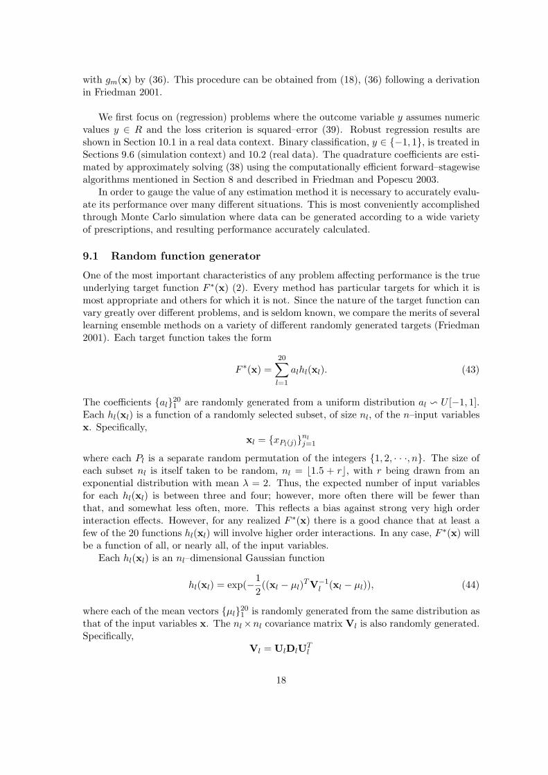
Figure 2: Distributions of standardized (left) and comparative (right) root mean squarederror for several bagged and corresponding post–processed bagged ensembles (suffix “P”)over the 100 data sets in the regression Monte Carlo study. Post-processing provides thegreatest improvement for the most diverse ensembles based on the weakest base learners.

stage, as well as for all sequential ensembles a separate set, from the training data, is leftaside for model selection. The resulting distributions of (46) (47) over the 100 data sets foreach method are summarized by boxplots.

9.3 Bagged ISLEs

Figure 2 displays results for various bagged tree ensembles and post-processed bagged en-sembles. One can see, in the plot of relative root–mean–square error (46) distributions (leftpanel), that the 100 targets represent a fairly wide spectrum of difficulty for all the meth-ods. The right panel shows the comparative RMS error (47) among these methods. Bagginglarge trees (fully grown on the 10,000 observation bootstrap training set, labelled as Bag)does better than bagging trees built on small 5% samples without replacement (labelledas Bag 5% ), and much better than bagging shallow (six terminal node) trees built on 5%samples (Bag 6 5% ). For these methods the ensemble prediction is taken to be the averageof the individual base learner (tree) predictions. The respective adjacent distributions inFig. 2 with labels ending in suffix “P” represent results for the corresponding method usingthe estimated optimal quadrature coefficients (38) (“post–processing”). These results showthat with post–processing the relative ranking of the corresponding ensembles is reversed.Using the optimal estimated quadrature weights transforms the poorest performing ensem-ble (Bag 6 5% ) to being the best. Comparing (26) with (30), one sees that an ensembleof trees, each constructed on randomly drawn 5% samples, is far more diverse (larger σ

20

(25)) than the trees built on bootstrap samples. It will thus contain many trees that arenot highly relevant to predicting the outcome variable y. It will also likely contain sometrees that are highly relevant. Simple averaging gives all trees equal weight so that theless relevant trees dilute the effect of the more relevant ones. Post–processing the ensemblewith an l1 penalty (38) tends to assign larger coefficients (weights) to the relevant predictors(trees) thereby mitigating this dilution effect.

Another element that accounts for the larger dispersion is the size of the trees. Bag 5%uses the largest possible trees that can be built on a 5% sample. These are considerablysmaller than the large trees that can be built on a bootstrap sample, and therefore lesscorrelated with the response; this leads to a more diverse ensemble. Bag 6 5% uses sixterminal nodes trees, and thus provides even greater dispersion through this mechanism.

Post-processing with the l1 penalty provides the greatest improvement when the dis-persion of the ensemble is the greatest. For the case for shallow trees each fitted on 5%samples post-processing improved the accuracy of the ensemble by about 50%, ultimatelycausing it to be the most accurate of all the competitors shown in Fig. 2. It is importantto note that, besides being the most accurate, Bag 6 5% P brings a huge improvement inspeed as compared with the classic bagging of large trees. The generation of the ensembleis few hundreds times faster and subsequent prediction is roughly five times faster.

Post–processing bagged large trees (ensemble labelled Bag P) does not produce an im-provement in accuracy over straightforward bagging. The large trees are highly correlatedand the dispersion of the ensemble is low. Fitting the coefficients in the post–processingregression is a bias reduction technique where the l1 penalization reduces variance throughshrinkage and feature selection. These ingredients do not seem to help much in settingswhere each individual base learner (tree) has low bias, in this case comparable with the biasof the ensemble as a whole. The averaging involved in the classic bagging is an aggressivevariance reduction technique that is appropriate in the context of high variance and lowbias. The very large trees being highly correlated on the training set are roughly equallyrelevant as predictors; the l1 regularization is best suited when the predictors do not haveequal importance. In fact the best settings for the l1 penalty are sparse situations whererelatively few of the predictors have non-zero coefficients (Donoho et al. (1995). While thisregularization seems to be appropriate for the predictors from highly diverse ensembles likeBag 6 5%, it does not seem well suited for the large bagged trees.

9.4 Random Forests ISLEs

The left panel of Fig. 3 deals with random forests (RF ) like ensembles. At each split, dur-ing tree construction ns = blog2n + 1c input predictor variables are randomly selected (thedefault suggested by Breiman 2001) and the best split variable is chosen among them. Thisdefault is used in all the results of the simulation study and real data experiments. Post–processing (38) improves the classic random forests (RF ) that build large (fully grown onthe bootstrap samples) trees by around 10%, and the forests that build trees on 5% (withoutreplacement) of the data (RF 5% ) by 30%. The biggest improvement with post–processing(80%) is obtained, as with bagging, for the random forest ensemble using shallow (six ter-minal node) trees built on 5% of the data (RF 5% P), again making it the most accurateamong these competitors. The dispersion of the random forest ensembles is, overall, larger

21

1.0

1.2

1.4

1.6

1.8

2.0

2.2

2.4

RF RF_P RF_5% RF_5%_P RF_6_5% RF_6_5%_P

Com

parativ

e R

MS

E

rror

Random Forests Comparative RMS Error

1.0

1.1

1.2

1.3

1.4

Bag RF Bag_6_5%_P RF_6_5%_PC

om

pa

ra

tive

R

MS

E

rro

r

Bag/RF Comparative RMS Error

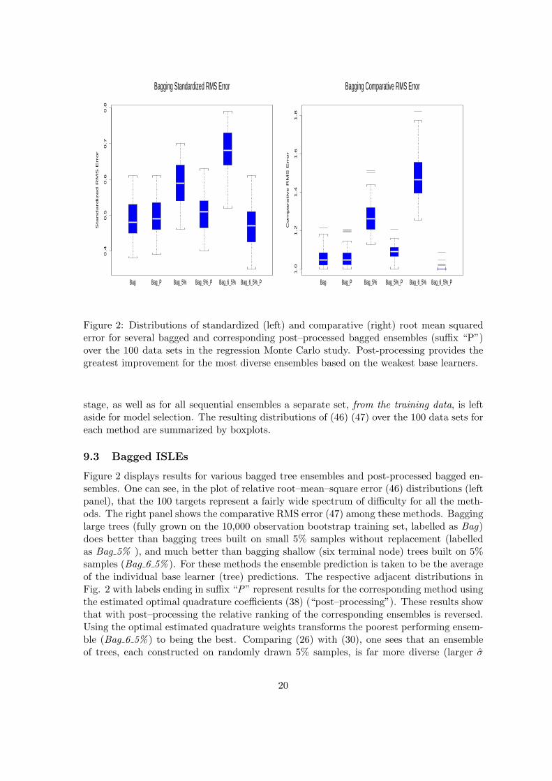
Figure 3: Distributions (left panel) of comparative root mean squared error over the 100data sets in the regression Monte Carlo study for various random forest ensembles andcorresponding post–processed ensembles (suffix “P”). Qualitative results are similar tothat of bagged ensembles (Fig. 2). The right panel compares results from selected baggedand random forest ensembles.

than that with bagging (as noted in Section (6.2)) and post-processing here provides moreimprovement.

Bagging, random forests, and their two corresponding fast post-processed winning en-sembles (Bag 6 5% P and RF 6 5% P) are compared on the right panel of Fig. 3. Herestraight bagging is better than random forests: the presence of the spurious variables seemsto limit the performance of the randomized trees that choose relatively small random sub-sets of features at each split. The degradation is even more pronounced when one dealswith shallow trees built on small fractions of data. This is the case with RF 6 5% (leftpanel). However, post-processing (RF 6 5% P) transforms this ensemble to be the overallwinner. It is also the overall winner in terms of training speed: it is more than 100 timesfaster than the classic random forests and more than 1,000 times faster than bagging.

9.5 Sequential ISLEs

The relative performance of several sequential ISLEs (Section 7.1) is displayed in the leftpanel of Fig. 4. The base learners for all sequential ISLEs are taken to be the small sixterminal nodes trees. The leftmost boxplot corresponds to the sequential ensemble Seq 0.1generated as in Section 7.2 with η = 0.1 in (18) (36). This is the default value giving rise

22

1.0

1.1

1.2

1.3

1.4

1.5

Seq_0.1 Seq_0.1_P Seq_0.01_10% Seq_0.01_10%_P Seq_0.01_20%_P

Co

mp

ara

tive

R

MS

Err

or

Err

or

Sequential ISLE: Comparative RMS Error

1.0

1.2

1.4

1.6

1.8

2.0

BaggLarg Bag_6_5%_P RF RF_6_5%_P SRF_10%_P Mart Seq.01_20%_P C

om

parativ

e R

MS

Bag/RF/Seq: Comparative RMS Error

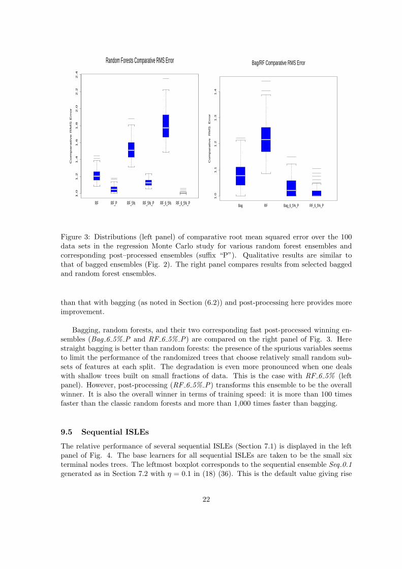
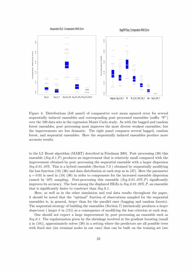
Figure 4: Distributions (left panel) of comparative root mean squared error for severalsequentially induced ensembles and corresponding post–processed ensembles (suffix “P”)over the 100 data sets in the regression Monte Carlo study. As with the bagged and randomforest ensembles, post–processing most improves the most diverse weakest ensembles, butthe improvements are less dramatic. The right panel compares several bagged, randomforest, and sequential ensembles. Here the sequentially induced ensembles produce moreaccurate results.

to the L2–Boost algorithm (MART) described in Friedman 2001. Post–processing (38) thisensemble (Seq 0.1 P) produces an improvement that is relatively small compared with theimprovement obtained by post–processing the sequential ensemble with a larger dispersionSeq 0.01 10%. This is a hybrid ensemble (Section 7.3 ) obtained by sequentially modifyingthe loss function (18) (36) and data distribution at each step as in (37). Here the parameterη = 0.01 is used in (18) (36) in order to compensate for the increased ensemble dispersioncaused by 10% sampling. Post-processing this ensemble (Seq 0.01 10% P) significantlyimproves its accuracy. The best among the displayed ISLEs is Seq 0.01 20% P, an ensemblethat is significantly faster to construct than Seq 0.1.

Here, as well as in the other simulation and real data results throughout the paper,it should be noted that the “optimal” fraction of observations sampled for the sequentialensembles is, in general, larger than for the parallel ones (bagging and random forests).The sequential strategy of building the ensembles (Section 7) intrinsically produces a largerdispersion ( larger σ in (15)) as a consequence of modifying the loss criterion at each step.

One should not expect a large improvement by post–processing an ensemble such asSeq 0.1. The regularization given by the shrinkage involved in the gradient boosting (smallη in (18)), approximately solves (38) in a setting where the predictors are all possible treeswith fixed size (six terminal nodes in our case) that can be built on the training set (see

23

Hastie, Tibshirani and Friedman 2001, Chapter 10.12.2). The approximation involves agreedy search strategy in place of an “optimal” exhaustive search for finding the best treeto add to the ensemble at each step. Here post–processing can help a little by re–adjustingthe coefficients for each tree. The hybrid strategies that sample data (and sometimes fea-tures as well) represent a further departure from the optimal exhaustive search. For thesestrategies post–processing can provide a dramatic improvement, often leading to higheraccuracy than the pure sequential approach.

The right plot of Fig. 4 shows an overall comparison for the parallel and sequentialensembles under study. The ensemble labelled Mart is the default L2–Boost (Friedman2001) MART algorithm that uses (39) as a loss function; it corresponds to the Seq 0.1 50%ensemble. The ensemble labelled SRF 10% P (sequential random features ISLE) is obtainedby post-processing a hybrid (Section 7.3) that perturbs all aspects of the problem: the datadistribution, by sampling 10% of the data at each step, the loss function as in (18) (36),and also the algorithm used to construct each individual tree, by sampling six features atrandom at each split as described in Section 6.2. The overall picture shows that here thesequential ISLEs tend to perform better than the parallel ones. This is consistent withresults observed in classical Monte Carlo integration where quasi-Monte carlo methodstend to outperform those based on purely random Monte Carlo sampling. In all casespost-processing the ensembles with large dispersion (large σ in (15)) tend to produce moreaccurate results.

9.6 Classification

To simulate an environment for testing the various types of ISLEs in a classification frame-work, 100 randomly generated target functions were simulated as in Section 9.1 and theclass labels (y ∈ {−1, 1}) were obtained by thresholding each target at its median. In thisway, 100 different training data sets of size 10,000 were obtained and the misclassificationerror rate for each ensemble under study was estimated on separate corresponding test setsof size 10,000. Although the Bayes error rate is zero for all of these problems, the decisionboundaries are fairly complex and the nature of the targets can make the classificationproblems difficult.

The sequential ISLEs are generated as in Section 7, using the loss criterion (41); thisloss was also used for post–processing all the ensembles. This criterion, unlike others usedfor classification such as the logistic–likelihood loss (Friedman 2001, Friedman, Hastie andTibshirani 2000) allows for updates that lead to a computationally fast and numericallystable post–processing algorithm (Friedman and Popescu 2003). When used in conjunctionwith η << 1 in (18) (36), the ramp loss (41) compares favorably to the logistic–likelihoodloss in terms of accuracy when generating the sequential ensembles.

As in Section 9.2, all sequential ISLEs use 6 terminal nodes trees. As before, whenfeatures are sampled, a subset of 6 out of 40 attributes are randomly selected at each split.

In general, the relative performance of the parallel and sequential classification ISLEsis similar to that obtained in the regression setting. The results closely correspond to theones presented in Sections 9.3–9.5 and summarized in Fig. 2–4. Figure 5 shows the overallpicture of various ISLEs for classification. In the left plot of the actual misclassification

24

0.0

60.0

80.1

00.1

20.1

40.1

60.1

80.2

0

Bag Bag_6_5%_P RF RF_6_5%_P Mart Seq_0.05_20%_P

Actu

al M

iscla

ssific

ation E

rror

ISLE for Classification: Misclassification Error

1.0

1.2

1.4

1.6

1.8

2.0

2.2

2.4

Bag Bag_6_5%_P RF RF_6_5%_P Mart Seq_0.05_20%_P C

om

parative M

iscla

ssific

ation E

rror

ISLE for Classification: Comparative Misclassification Error

Figure 5: Distributions of misclassification (left) and comparative (right) error rates forseveral bagged, random forrest, and sequential ensembles over the 100 data sets in theclassification Monte Carlo study. The results parallel those obtained in the regressionMonte Carlo study.

error rate it is seen that the degree of difficulty for the 100 problems varies. The right plotusing the analog of (47) facilitates a comparison among these methods. Random forestsare not as accurate as bagging, an artifact of the spurious variables; however the fast post–processed forest–like ensemble RF 6 5% P achieves the best accuracy among the parallelISLEs. The sequential ISLEs (quasi-Monte Carlo) are here much better than the parallelones. The ensemble labelled Mart corresponds to a sequential ensemble generated withthe logistic–likelihood loss (the algorithm K2–Boost from Friedman 2001). Here the overallwinner is Seq 0.05 20% P, being slightly more accurate than MART.

10 Real Data Experiments

This section presents experiments on actual data. Five hundred trees were generated foreach ensemble. Shallow tree base learners have ten terminal nodes, while the large trees usedfor classic bagging and random forests are fully grown. For random forests the number ofrandom features are always taken to be blog2n+1c, where n is the total number of features,as suggested in Breiman 2001.

25

Algorithm/MAE (2· stdev) data target=RF target=MARTBagging 0.563(0.008) 0.328(0.013) 0.465(0.007)Bagging P 0.552(0.008) 0.375(0.005) 0.378(0.011)Bagging 10 nodes 5% 0.885 (0.016) 0.550(0.010) 0.756(0.013)Bagging 10 nodes 5% P 0.537 (0.010) 0.321(0.006) 0.274(0.007)Random Forests 0.560 (0.008) 0.272(0.013) 0.500(0.007)Random Forests P 0.502 (0.008) 0.312(0.013) 0.344(0.007)RF 10 nodes 5 % 0.863 (0.014) 0.592(0.010) 0.779(0.011)RF 10 nodes 5 % P 0.495 (0.014) 0.297(0.009) 0.222(0.006)MART 0.473(0.009) 0.280(0.005) 0.145(0.002)Seq 0.01 5% 0.615(0.010) 0.429(0.009) 0.492(0.015)Seq 0.01 5% P 0.487(0.020) 0.301(0.007) 0.173(0.003)

Table 1: Scaled median absolute error of several bagged, random forest, and sequentiallyinduced ensembles, along with their corresponding post–processed counterparts (suffix “P”)on the census data (second column). Qualitatively, the results reflect those obtained inthe regression Monte Carlo study. The third and fourth columns respectively representcorresponding results for the random forest and MART created target functions (see text).Most ensembles do comparatively well on the random forest generated target, whereasthe sequentially induced ensembles seem to have a competitive edge on the MART targetfunction.

10.1 Robust regression: census data

The data set used here was obtained from the IPUMS (http://www.ipums.umn.edu/usa)census database. There are 71 variables selected from the 2000 Supplementary Survey(CS2SS). The goal here is to predict the total personal income of a given individual from theother 70 variables. These consist of a mixture of categorical (e.g. “occupation”, “industry”)and of orderable (e.g. “grade level attending”, “family size”) features. There are manymissing values. The dataset is an IPUMS sample of size 46,937 from the United Statespopulation. The observations come with individual weights that reflect the distribution ofthe United States population. These weights are used both in training and in reporting theresults.

Unlike the datasets presented in the simulation study, severe response (income) out-liers were present in the census data. Therefore, the Huber-M loss (40) was used in thepost-processing as well as in generating the sequential ensembles (following the genericmethodology described in Section 7). Also the test error reported in every case is thescaled median absolute error (MAE):

MAE = median(y − y)/median(y −median(y)). (48)

The data set was randomly partitioned into a learning (training) set consisting of 36,000and a test set of 10,937 observations. The quantities from Table 1 are test errors averagedover five such partitions. The numbers in parentheses are two times the standard deviationsof the means that assess the significance of the differences. The error of a single ten node

26

tree is 0.805 (0.041) and the error of the largest possible tree grown on the training data is0.687 (0.006).

The second column in Table 1 present the results obtained by various ISLE methods(first column) on these data. The post–processed ensembles performances are shown initalics. The results are consistent with those from the simulation study. The largest im-provement by post-processing (38) among the parallel (bagging and random forest) ISLEsappears for the ensembles with the highest dispersion that employ shallow (10 nodes) trees,each built on 5% of the data (improvement of 65% for bagging and 74% for random forests).The overall winner among these parallel ISLEs is a fast post-processed random forest en-semble that builds shallow trees on small fractions (5%) of the data. The sequential ISLESeq 0.01 5% P that generates 10 terminal node trees built each on 5% samples with the lossfunction (40) performs comparably in accuracy with MART (the algorithm Huber–M–Boostof Friedman 2001). As in the simulation study, the sequential (quasi Monte Carlo) ISLEsappear to have a performance edge, but the differences here are much less pronounced.

It is important to note that measure (48), unlike (46), includes the irreducible errorε (45), and, therefore, the fractional differences in estimating the actual underlying tar-get function are much greater. In order to get an idea of such differences, two “target”functions were defined on these data. The first is taken to be the random forest approxima-tion, F ∗

1 (x) = FRF (x), obtained on the census data as averaged over the five replications(learning–test partitions). The second target is the Seq 0.1 50% (MART) approximationF ∗

2 (x) = FMART (x), obtained in the same manner. For each of these targets five data sets{yi,xi}N

1 were constructed by forming the residuals from the corresponding target

{ril = yi − F ∗l (xi)}N

i=1, l = 1, 2, (49)

randomly permuting them among the observations, and then adding them to each corre-sponding target value

{yil = F ∗l (xi) + rP (i)l}N

i=1 , l = 1, 2. (50)

Here P (·) is a random permutation of the integers {1, ..., N}. This process was repeatedfive times with five different random perturbations.

The last two columns of Table 1 show the scaled median error in approximating thesetwo targets

median[F ∗l (x)− Fl(x)]/median[F ∗

l (x)−median(F ∗l (x))], l = 1, 2,

as averaged over the five replications. Here Fl(x) represents the approximation obtained bythe respective methods as applied to the “data” (49) (50), constructed from F ∗

l (x), l = 1, 2.

As would be expected the sequential ISLEs (including MART) perform best when ap-proximating the MART target function F ∗

2 (x). The parallel ISLEs based on bagging andrandom forests do relatively poorly when compared to the sequential ones. Nevertheless,post–processing brings significant improvements. For example, post–processing the fastrandom forest ensemble that builds shallow trees on 5% samples leads to an ISLE that ismore than tree times as accurate as the corresponding non post–processed ensemble, and

27

more than twice as accurate as the classic random forest ensemble!

For the random forest target function F ∗1 (x), the parallel ISLEs perform relatively well

(especially random forests itself). However the sequential ISLEs also tend to do compara-tively well on the random forest target function.

MART produces approximations that emphasize low order interactions and, when ap-propriate, relatively few input predictors variables. By contrast random forests tend toproduce higher order interaction models involving many predictors. The correspondingderived targets F ∗

2 (x) and F ∗1 (x) will reflect these properties. The results shown in the

last two columns of Table 1 suggest that sequential ISLEs achieve their greatest advan-tage for low interaction targets involving relatively few relevant predictor variables. Thiswas the case for the simulation study presented in Section 9. In situations where the trueunderlying target function F ∗(x) (2) tends to involve many relevant variables and/or highorder interactions, the sequential ISLE strategy does not seem to have an advantage (nordisadvantage) with respect to the parallel ISLEs based on bagging and random forests.

10.2 Classification: spam 2003 data

The spam prediction problem considered here has its goal to discriminate the spam emailsfrom the non-spam ones. The database consists in 19,177 emails. Each email is charac-terized by 833 binary features among which are the presence in the email text of variousstrings like “cash bonus”, “guarantee”, characteristics of the email header such as InvalidDate or “From” yahoo.com does not match “Received” headers, URL features such as: Usesa numeric IP address in URL or Uses non-standard port number for HTTP etc. Detailsand the actual dataset are available at http://www.data-mining-cup.com/.

A test set of 4,000 emails was randomly chosen; the remaining emails were used fortraining each ensemble. This experiment was repeated five times with different randompartitions. The sequential ensembles for the classification experiments in this section aregenerated as in Section 7 using the least-squares ramp loss function (41). The same lossfunction is also used in post–processing for all the ensembles.

Table 2 presents the test misclassification errors (average and two standard deviations).Although the base error (predicting majority class) is 39%, many of the ensembles consid-ered here achieve very low misclassification errors (less than 0.01=1%). The misclassifica-tion error of a single 10 terminal nodes tree is 0.0303 (2 · stdev = 0.0008) and the errorfor a 15,177 terminal node tree (the largest possible trees that can be built on the trainingdata) is 0.0120 (2 · stdev = 0.0012).

One can see from Table 2 that the ensemble Bag 10 1% P obtained from postprocess-ing the widely dispersed ensemble using 10 terminal node trees built on 1% subsamples(Bag 10 1% ) produces an improvement by a factor of three and comes close to the errorrate achieved by bagging large trees while being 700 times faster to construct.

The random forests use 10 out of the total of 833 features randomly sampled at eachsplit. Post–processing random forests helps; the improvement in accuracy is dramatic when

28

Algorithm Error(2·stdev)Bagging 0.0085(0.0011)Bagging P 0.0089(0.0012)Bagging 10 nodes 1% 0.0327(0.0013)Bagging 10 nodes 1% P 0.0103(0.0020)Random Forests 0.0147(0.0012)Random Forests P 0.0086(0.0011)RF 10 nodes 1% 0.0837(0.0048)RF 10 nodes 1 % P 0.0091(0.0010)Seq 0.1 50% 0.0083(0.0005)Seq 0.01 5% 0.0120(0.0013)Seq 0.01 5% P 0.0080(0.0010)SRF 0.01 5% 0.0256(0.0016)SRF 0.01 5% P 0.0084(0.0006)

Table 2: Misclassification error rates of various ensembles and their post–processed coun-terparts (suffix “P”) on the spam 2003 data. Error rates for all methods are quite small.Bagging and all fast post–processed ensembles have comparable performance.

post–processing the ensemble RF 10 1% : here a factor of nine! The ensemble RF 10 1% Pthat is competitive with the best ensembles in Table 2 builds 10 terminal nodes trees ononly 1% of the data while selecting at each split a very small fraction of features. Fur-thermore, ensemble construction based on bagging and random forests can be parallelized,thereby allowing training to be done on databases involving a huge number of emails. Post-processing helps the sequential ensembles built on small fraction of the data (5%) (as it isthe case for Seq 0.01 5% ) and leads to a big improvement (a factor of three) for the hybridSRF 0.01 5% that sequentially builds randomized trees (10 random features at each split)on 5% of the data.

Unlike the simulation examples (Section 9.6), and the census regression problem (Section10.1) in the real data classification example presented here there is no signifficant differencebetween the best parallel and sequential ensembles. Here the ISLE methodology producesoverall competitive ensembles in terms of accuracy while giving rise to huge computationalreductions in training time. The post-processed ensembles also have a substantial advantagein time required for subsequent prediction (see below). This can be very important forservers that receive email messages at high rates.

The fractions used here for sampling the training data (1% for the parallel ISLEs and5% for the sequential ones) are smaller than those used in Section 9.3. This is due to thelarger sized training data sets involved (see Section 5.1).

11 Discussion

A two–stage strategy for creating a final model has been previously considered in the contextof prediction ensembles. Breiman 1996b suggests forming linear combinations of variouslearners to improve accuracy. This methodology has its roots in the idea of stacking, intro-

29

duced in Wolpert 1992. The stacking methodology is used also in Wolpert and Macready1996. They employ various post–processing strategies applied to classic regression baggedensembles (built on bootstrap samples) and report improvements in accuracy when com-pared with classic bagging.

The present paper presents classic ensemble prediction methodologies such as bagging,random forests, boosting (and bayesian model averaging) in a unifying framework basedon numerical integration with importance sampling. This helps explain some of their prop-erties. In particular, the empirically observed trade-off between the strength of individualbase learners and the correlations among them (Breiman 2001) is related to the width ofthe corresponding parameter sampling distribution (15) used by the integration rule (9). Itis seen that estimating the optimal coefficients (10) for the integration rule through (38),rather than simply averaging the integrand values, allows for the use of much weaker lesscorrelated base learners (more diverse ensembles), often leading to substantial gains in pre-diction accuracy and dramatic reductions in training time. As in classical Monte Carlointegration, the sequential strategy (Section 7) corresponding to quasi Monte Carlo tendsto outperform the parallel strategy (Section 6) that corresponds to purely random samplingMonte Carlo. However, the parallel implementation can result in a strong computationaladvantage for very large data sets.

Estimating the optimal coefficients through (38) also results in reduced computationfor subsequent predictions; the regularized l1 regression-like algorithms used for post–processing produce sparse models, with many zero coefficients. Therefore, the correspond-ing (zero coefficient) base learners need not be evaluated for prediction. Another ingredientthat helps here is the use of the shallow trees with a considerably faster look-up speed thanthe large trees used in ensembles like bagging or random forests. Prediction speed can bevery important for some real time applications (e.g. spam recognition, fraud detection,automatic target recognition etc).

The methodology presented in this paper is not restricted to decision tree ensembles.One could use the ISLE methodology to create ensembles formed by sigmoids of linear com-binations of the predictor variables (6), or radial basis functions, thereby creating singlelayer neural or radial basis function networks. One could combine base learners from differ-ent classes (trees, linear functions of the original features, sigmoids, etc) to obtain MISLEs(Multiple Importance Sampled Learning Ensembles). This can be especially useful whenthe base learners from a given class have difficulty in estimating particular functional (input-output) dependencies.

Finally, it should be noted that all comparisons presented in this paper (Sections 9 and10) are made on moderate to large data sets (number of observations) commonly encoun-tered in data mining applications. It is in these settings that the computational advantagesassociated with the post–processing strategy achieve their greatest significance. The partic-ular trade–offs suggested by these examples may or may not extend to applications involvingrelatively small data sets.

30

12 Acknowledgements

The work of Jerome Friedman was partially supported by the Department of Energy undercontract DE-AC03-76SF00515 and the National Science Foundation under grant DMS-97-64431. The work of Bogdan Popescu was partially supported by the National ScienceFoundation under grant DMS-97-64431.

References

[1] Breiman,L. (1996a). Bagging Predictors. Machine Learning, 26 123-140.

[2] Breiman,L. (1996b). Stacked Regressions. Machine Learning, 24 51-64.

[3] Breiman,L. (2001). Random Forests, random features. Technical Report, University of Califor-nia, Berkeley.

[4] Breiman,L., Friedman, J. H., Olshen, R., and Stone, C. (1983). Classification and RegressionTrees. Wadsworth.

[5] Freund, Y. and Scahpire, R.E. (1996). Experiments with a new boosting algorithm. MachineLearning: Proceedings of the Thirteenth International Conference, Morgan Kauffman, San Fran-cisco, 148-156.

[6] Copas, J. B. (1983). Regression, prediction and shrinkage (with discussion). J.R. Statist. Soc.B 45, 311-354.

[7] Chipman H., George E., McCullagh R. (1998). Bayesian CART model search (with discussion).Journal of Am. Stat. Assoc. 93 (6), 937-960.

[8] Denison, D. G. T., Holmes, C. C. , Mallik, B. K. and Smith, A. F. M. (2002). Bayesian nonlinearmethods for classification and regression. Chichester: John Wiley.

[9] Dietterich, T. G. (2000). An experimental comparison of three methods for constructing en-sembles of decision trees: bagging, boosting and randomization. Machine Learning, 40 (2)139-158.

[10] Donoho, D., Johnstone, I. (1993). Ideal spatial adapdation by wavelet shrinkage. Biometrika81, 425-455.

[11] Donoho, D., Johnstone, I., Kerkuacharian, G. and Picard, D. (1995) Wavelet shrinkage; asymp-totya? (with discussion). J. Royal. Statist. Soc 57: 201-337.

[12] Efron, B. and Tibshirani, R. (1993). An introduction to the bootstrap, Chapman and Hall,London.

[13] Efron, B., Hastie, T., Johnstone, I. and Tibshirani, R. (2002). Least Angle Regression. Annalsof Statistics. To appear.

[14] Friedman, J. H. (2001). Greedy function approximation: A gradient boosting machine. Annalsof Statistics, Vol. 29, No. 5.

[15] Friedman, J. H., Hastie, T. and Tibshirani, R. (2000). Additive logistic regression: a statisticalview of boosting (with discussion). Annals of Statistics, 28, 337-407.

[16] Friedman, J. H., and Popescu, B. E. (2003). Gradient directed regularization for regression andclassification. Stanford University, Department of Statistics. Preprint.

[17] Hastie, T., Tibshirani, R. and Friedman, J.H. (2001). Elements of Statistical Learning.Springer-Verlag.

31

[18] Ho, T. K. (1995). Random Decision Forests. Proceedings of the 3rd International Conferenceon Document Analysis and Recognition 278-282.

[19] Hoerl, A. E. and Kennard, R. (1970). Ridge Regression: Biased estimation for nonorthogonalproblems. Technometrics 12, 55-67.

[20] Huber, P. (1964). Robust estimation of a location parameter Annals of Math. Stat, 53, 73-101.

[21] Popescu,B.E. (2003). Ensemble Learning. Ph.D Thesis. Stanford University.

[22] Quinlan, R. (1991). C4.5: Programs for Machine Learning. Morgan Kaufmann, San Mateo.

[23] Rumelhart, D.E.,Hinton, G. E., Williams, R. J. (1986). Learning representations by back-propagating errors. Nature 323, 533-536.

[24] Schapire, R. and Singer, Y. (1998). Improved boosting algorithms using confidence-rated pre-dictions. Proceedings of the Eleventh Annual Conference on Computational Learning Theory.

[25] Stroud (1971). Approximate calculation of multiple integrals. Prentice Hall, Englewood Cliffs,New Jersey.

[26] Tibshirani, R. (1996). Regression shrinkage and selection via the lasso J. Royal. Statist. Soc.B. 58: 267-288.

[27] Wolpert, D. H. (1992). Stacked Generalization Neural Networks 5: 241-259.

[28] Wolpert, D. H. and Macready W. G. (1996). Combining stacking with bagging to improve alearning algorithm. Technical Report SFI-TR-96-03-123, Santa Fe Institute, Santa Fe, NewMexico.

32