Impacts of Data Call Characteristics on

Multi-Service CDMA System Capacity

Yujing Wu, Carey Williamson

Department of Computer Science, University of Calgary,2500 University Drive NW, Calgary, AB, Canada T2N1N4

Abstract

The capacity of multi-service Code-Division Multiple Access (CDMA) systems hasbeen extensively studied in the literature. However, few studies address the funda-mental issue of how the stochastic properties of non-Poisson data traffic affect thesystem capacity. This paper studies a CDMA system supporting voice and datatraffic. Results show that increased variability in the data call arrival process de-creases the system capacity, while increased variability in data call holding timesincreases the system capacity. The extent of these effects depends on other systemparameters, such as transmission rates and communication quality requirements.These observations motivate a simple buffer-based resource management schemethat enhances the system capacity in the presence of high-variability data traf-fic, providing controllable performance tradeoffs between voice and data calls. Thisstudy uses both simulation and theoretical analysis, which is based on a MarkovRegenerative Process (MRGP) model.

Key words: CDMA, Capacity Planning, Loss System, Markov RegenerativeProcess, Variability of Stochastic Processes

1 Introduction

Mobile service providers have recently made substantial investments to deploy3G CDMA networks in North America. For example, CDMA2000 1xRTT net-works have been available for several years, while data-optimized CDMA20001xEV-DO networks are being rolled out now.

Email address: ywu,carey@cpsc.ucalgary.ca(Yujing Wu, Carey Williamson).

Preprint submitted to Elsevier Science 20 June 2005

Despite the large-scale and rapid deployment of these networks, capacityplanning for CDMA data networks is not well understood. Current planningonly supports the availability of high-speed data services. However, given thegrowth trends in data traffic volume and the inherent scarcity of radio spec-trum resources, better capacity planning tools are required.

In voice-only 2G cellular networks, the Erlang B formula has been used forcapacity planning for many years. The success of this simple tool lies in thefact that voice traffic is well-modeled by a Poisson process. Internet-like datatraffic, however, exhibits high variability over many timescales, which is notconducive to Poisson-based modeling [12]. This makes capacity planning in3G networks a challenging task.

Current research on multi-service CDMA network capacity falls into two maincategories. The first category is the analytical approach [1,2,5,6,8]. In most ofthese models, data traffic differs from voice traffic only in the transmission rateand quality of service (QoS) requirements, not in the stochastic traffic behav-ior. The Poisson assumption is still made for the data call arrival process. Thesecond category is the simulation approach. Traffic generators are integratedinto the simulation environment, which models the CDMA protocol stack andthe radio channel. Traffic models are used to emulate data applications, suchas WWW, email, and WAP. Simulation results show the relationship betweenoffered traffic load and required radio resources. These two types of stud-ies, however, have not addressed the fundamental issue of how the stochasticproperties of non-Poisson data traffic affect the overall system capacity.

In this paper, we study a multi-service CDMA system supporting voice andnon-Poisson data traffic over dedicated channels. Our results show that thevariability of the data call arrival process adversely affects the system capacity,while the variability of data call holding times increases the system capacity.The extent of these effects depends on system configurations, such as trafficmix, transmission rates, and QoS requirements. Based on these observations,we propose and evaluate a simple buffer-based resource management schemethat effectively increases the system capacity in the presence of high-variabilitydata traffic. Our study is carried out by simulation and theoretical analysisbased on a Markov Regenerative Process (MRGP) model.

The rest of the paper is structured as follows. Section 2 introduces the keyconcepts of CDMA network capacity and the system model. Section 3 presentsthe analytic study for a simple system. Section 4 is devoted to the simulationstudy for a more general model. Section 5 presents and evaluates the data callbuffering scheme. Finally, Section 6 concludes the paper.

2

2 Capacity and System Model

2.1 CDMA Network Capacity

A CDMA network consists of base stations (BS) each providing service tomobile stations (MS). Transmissions from the home BS to a MS traverse theforward link, while transmissions from a MS to the home BS traverse thereverse link.

One of the principal characteristics of a CDMA network is that the capacityin each direction depends on the total interference experienced by an MSor the BS. The interference level depends on the cell layout, the MS spatialdistribution, and the radio propagation characteristics. To facilitate capacityanalysis, an approximate model for the interference is often employed. Theapproximation is based on the following assumptions: the network cells arehomogeneous; the MSs are uniformly placed within the cell; Rayleigh fadingis ignored; and shadow fading is modeled by the lognormal distribution.

This paper uses two types of capacity measures. The first one, referred toas the capacity bound, is the maximum number of concurrent users that thesystem can support at a specified transmission rate and communication qualityEb/No (the ratio of bit energy to noise plus interference density). The boundis calculated assuming a fixed number of active MSs in each traffic class. Thesecond type of measure, referred to as Erlang capacity, is the average trafficload that can be supported at a given communication quality and serviceavailability probability. The Erlang capacity is evaluated in a dynamic userscenario, with calls initiated and terminated according to stochastic processes.Next we summarize the capacity bounds for the reverse and forward links, andthen discuss the relationship between the Erlang capacity and a loss system.

We introduce common notation for the analysis of both link directions. Assumethat the system supports N > 1 traffic classes. For the i-th class, let ni

be the number of active users, ri be the transmission bit rate, αi be thetraffic activity factor, and ηi be the required Eb/No. Let W be the spreadingbandwidth, and let Q−1(x) denote the inverse Q-function defined by Q(x) =∫∞x (1/

√2πe−y2/2)dy.

The reverse-link capacity bound [2,8] is given by:

N−1∑

i=0

niriαiηi ≤⟨

1

1 + f

⟩

W × 10Q−1(β)σx/10.0−aσ2x (1)

where 〈 11+f

〉 is the average frequency reuse factor, σx is the standard devia-

tion of the received signal to noise power ratio (SIR) in dB, a is a constant

3

with typical value 0.012, and β is the required system reliability such thatPr ((Eb/No)i ≥ ηi) = β. The term 10Q−1(β)σx/10.0−aσ2

x reflects the impact ofthe power control error. The standard deviation σx has a typical value be-tween 0.3 dB and 2 dB.

Next, we express the forward-link capacity bound based on the work by Leeet al. [10]. Let Pi represent the BS transmission power for a class i MS at thecell edge, and Ptot be the total transmission power of the home BS. The Eb/No

for a class i MS at the edge of the cell must satisfy:

(

Eb

No

)

i

=W

ri

Pi

KfPtot≥ ηi × 10−

Q−1(β)σy

10 , (2)

where σy is the standard deviation of the lognormally distributed propaga-tion loss in dB, β is the required system reliability and Kf is the ratio ofthe received power at the edge MS from other cells and from the home cell.Typically, Kf = 2.778. The transmission power at the home BS satisfies:Ptot = Kt

∑N−1i=0 niαiPi, where the average forward-link power factor Kt < 1

accounts for the fact that not all MSs are located at the cell boundary (i.e.,closer MSs require less BS transmission power). We assume that Ptot is notlarger than the BS power limit [10]. The maximum number of users are sup-ported when constraint (2) achieves equality. The forward-link capacity boundis given by:

N−1∑

i=0

niriαiηi ≤W

KfKt10Q−1(β)σy/10.0 . (3)

The capacity bounds in each direction (1) and (3) have the common form:

N−1∑

i=0

niwi ≤ ξ , (4)

where ξ > 0, wi > 0, and ni ≥ 0, ∀i = 0, . . . , N − 1. The right hand side of (4)can be viewed as the total system effective bandwidth and wi as the effectivebandwidth required by a call of the i-th class. The effective bandwidth dependson the assigned transmission rate, traffic activity factor, and required Eb/No.An admissible state (n0, . . . , nN−1) satisfies the bound (4). The admissionregion Ω is the set of all admissible states. A call arrival that would movethe system state out of the admissible region is blocked and cleared from thesystem. Otherwise, the call is accepted, and it consumes its effective bandwidthfor the holding time of the call. The maximum tolerable blocking probabilityof the system determines the average traffic load that can be accommodated.This probability can be a maximum aggregate blocking probability, or a vectorwhere the ith element is the maximum blocking probability for class i. Erlangcapacity can be expressed as an arrival rate vector producing the maximumtolerable blocking probability.

4

By using the capacity bounds, we convert the capacity analysis in either direc-tion of a CDMA system to the study of a loss system, where multiple trafficclasses completely share the resources subject to the admission requirement(4). Modeling a CDMA cell as a loss system is not new. Several authors haveused this approach especially for the reverse-link capacity analysis [1,2,6,7].Many of these studies assume that the call arrival process for each class isPoisson, and then model the system as a multi-dimensional continuous timeMarkov chain.

A Poisson arrival process may adequately model data traffic at the sessionlevel [12]. However, CDMA data calls do not necessarily correspond to suchsessions. For example, consider Web browsing in a CDMA2000 1xRTT system.A down-link data call may transmit a Web page or several successive Webobjects. The arrival process of data calls is not that of browsing sessions. Sincedata traffic exhibits high variability over many timescales, it is questionableto use the Poisson model for the traffic at levels other than the session level.In this paper, we assess the impact of non-Poisson data traffic on the CDMAsystem capacity.

2.2 System Model

There is a correspondence between the Erlang capacity of a multi-serviceCDMA system and a loss system. As a consequence, we study a loss sys-tem whose parameters are configured based on the capacity bounds of theCDMA system. Specifically, the system is characterized as follows:

• The system supports two types of calls: data (class 0) and voice (class 1).They have different transmission rates ri and Eb/No requirements ηi.

• Data calls are generated as a renewal process with rate λ0. The inter-arrivaltime X0 has a general cumulative distribution function G(x). The numberof bits Y0 transmitted by a data call, referred to as the workload size, is ani.i.d. random variable with a general distribution.

• Voice calls are generated according to a Poisson process with rate λ1, andhave exponentially distributed workload sizes Y1.

• Once a call is accepted into the system, it remains in the system for durationYi/(riαi), where αi is the traffic activity factor. The mean service rate forclass i calls is µi, where µi = riαi/E[Yi].

Table 1 lists the model parameters for the forward link. Substituting the corre-sponding values into (3), the capacity bound is obtained. All simulations andnumerical studies use the values listed in Table 1 unless otherwise specified.The mean workload size of voice calls is based on a mean call holding time of120 seconds, a typical value in cellular networks. The mean workload size of

5

Table 1Model Parameters

System parameters Value

Spreading bandwidth W 1.2288 MHz

Kf 2.778

Kt 0.35

σy 0

Traffic parameters Data calls (Class 0) Voice calls (Class 1)

Transmission rate ri (kbps) 100 9.6

Traffic activity factor αi 1.0 0.5

Eb/No requirement ηi (dB) 3 4

Arrival rate ratio λi

λ0+λ120% 80%

Mean workload size E[Yi] (bits) 440,000 576,000

Target blocking (case I) aggregate blocking 2%

Target blocking (case II) 5% 2%

data calls is based on a mean Web page size of about 50 KB. We assume that80% of the calls offered to the system are voice calls, and 20% are data calls.Since this ratio is fixed, the maximum aggregate arrival rate denoted by Λ de-termines the Erlang capacity as [0.2Λ, 0.8Λ]. We use this maximum aggregaterate to indicate the system capacity, and all the following studies are based onthis performance measure. We consider two different blocking requirements asindicated in Table 1. The first case concerns the overall blocking rate whilethe second case considers class-specific blocking rates.

Our study focuses on the impact of the variability of inter-arrival times X0

and workload sizes Y0 of data calls. Coefficient of Variation (CV) is a measureof variability for a random variable. CV is defined as the ratio of the standarddeviation to the mean. Let ca (arrival) and cs (size) denote the CV of X0 andY0, respectively. Our studies illustrate the relationship between the systemcapacity Λ and these two parameters. We use second-order hyperexponentialdistributions to model interarrival times and workload sizes with CV > 1.

3 Theoretical Analysis via MRGP

We use a Markov Regenerative Process (MRGP) to study the system describedin Section 2.2. However, there is a restriction on the data call model: the

6

holding time must be exponentially distributed. We leave the study of a moregeneral system to Section 4, where simulation is used.

Trivedi et al. [3] developed solution methods for MRGPs, and applied themto the performance and reliability analysis of various computer systems. Ourstudy is another effort along this line. For the details of MRGP theory andsolution techniques, the reader may refer to [4,9]. We briefly introduce theMRGP technical background here, and then describe the MRGP model for asimple CDMA system.

3.1 Introduction to MRGP

In a MRGP, there exist time points where the process satisfies the Markovproperty [3]. These time points are referred to as regeneration points. Thestochastic evolution between two successive regeneration points depends onlyon the state at regeneration, not on the evolution before regeneration. Further-more, due to the time homogeneity of the embedded Markov renewal process,the evolution of the MRGP becomes a probabilistic replica after each regener-ation. The key concepts of MRGP are given in the following two definitions [3].

Definition 3.1 A sequence of bivariate random variables (un, tn), n ≥ 0 iscalled a Markov renewal sequence if: (I) t0 = 0, tn+1 ≥ tn; un ∈ Ψ ⊂ Ω, whereΩ is a countable set represented by 0, 1, 2, . . .; and (II) ∀n ≥ 0,

Pun+1 = j, tn+1 − tn ≤ t|un = i, tn, . . . , u0, t0= Pun+1 = j, tn+1 − tn ≤ t|un = i (Markov property)

= Pu1 = j, t1 ≤ t|u0 = i (time homogeneity).

(5)

Definition 3.2 A stochastic process z(t), t ≥ 0 on Ω is called a Markovregenerative process if there exists a Markov renewal sequence (un; tn), n ≥ 0of random variables such that all conditional finite-dimensional distributionsof z(tn + t); t ≥ 0 given z(v); 0 ≤ v ≤ tn; un = i are the same as those ofz(t), t ≥ 0 given u0 = i, i ∈ Ψ ⊂ Ω.

The above definition implies that z(t+n ), n ≥ 0 or z(t−n ), n ≥ 0 is anembedded Markov chain (EMC), and that tn is a regeneration point of z(t).

The global kernel K(t) and the local kernel E(t) determine the evolution of aMRGP. Kernel K(t) describes the behavior of z(t) at the regeneration instantswhile kernel E(t) describes it between two consecutive regeneration instants.Entries of matrix K(t) = [Ki;j(t)], i, j ∈ Ψ, are given by (5). Matrix K(∞)is the one-step transition probability matrix of the EMC. Entries of matrixE(t) = [Ei;j(t)], i ∈ Ψ, j ∈ Ω, are given by Ei;j(t) = Pz(t) = j, t1 > t|u0 =

7

i . If local state transitions (between two consecutive regeneration points)are governed by a homogenous continuous time Markov chain (CTMC), theMRGP has a subordinate CTMC.

Knowledge of the kernels allows us to obtain three new variables, which lead tothe solution of the steady state probabilities of the MRGP. The first variableαi;j is given by

αi;j =∫ ∞

0Ei;j(τ)dτ , i ∈ Ψ, j ∈ Ω . (6)

This variable is the mean time that z(t) spends in state j between two suc-cessive regeneration instants, given that it started in state i after the lastregeneration. The second one is defined as βi = E[t1|u0 = i], i ∈ Ψ . It is themean duration of the next state of the renewal sequence given that the currentstate is i. The third variable is the steady state probability vector ~ν = (νk) ofthe EMC, which satisfies:

~ν = ~νK(∞),∑

k∈Ψ

νk = 1. (7)

Theorem 1 in the book by Kulkarni [9] gives the steady state probabilities ofthe MRGP based on αi;j, βi and ~ν.

3.2 MRGP Analysis of a CDMA System

3.2.1 MRGP Model

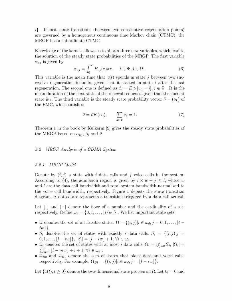
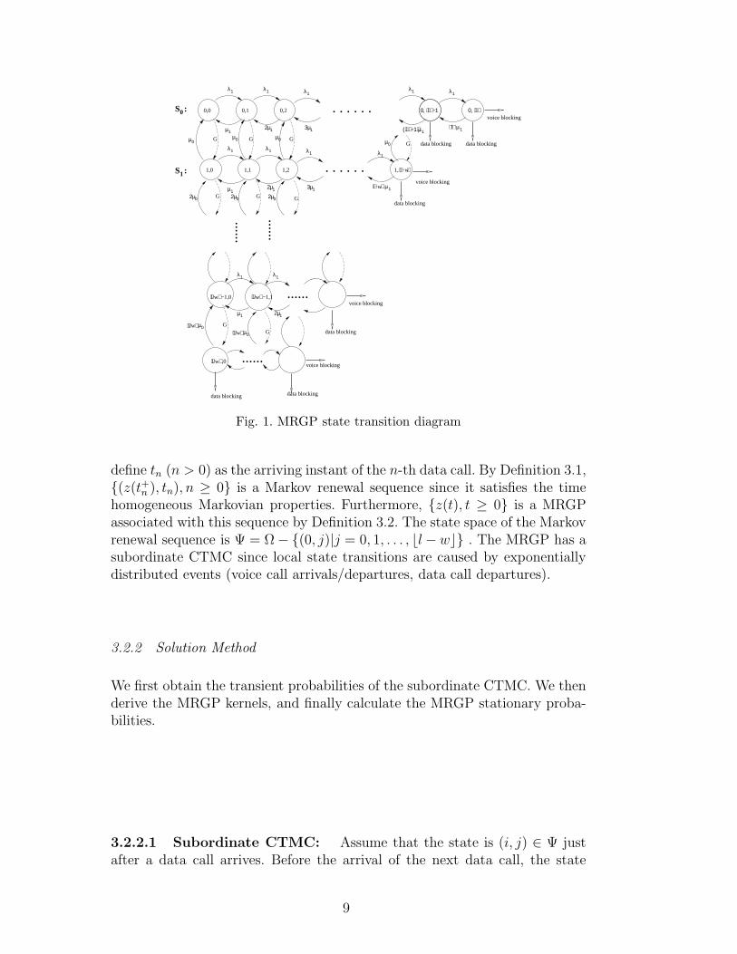
Denote by (i, j) a state with i data calls and j voice calls in the system.According to (4), the admission region is given by i × w + j ≤ l, where wand l are the data call bandwidth and total system bandwidth normalized tothe voice call bandwidth, respectively. Figure 1 depicts the state transitiondiagram. A dotted arc represents a transition triggered by a data call arrival.

Let b·c and | · | denote the floor of a number and the cardinality of a set,respectively. Define ωd = 0, 1, . . . , bl/wc . We list important state sets:

• Ω denotes the set of all feasible states. Ω = (i, j)|i ∈ ωd, j = 0, 1, . . . , bl −iwc.

• Si denotes the set of states with exactly i data calls. Si = (i, j)|j =0, 1, . . . , bl − iwc, |Si| = bl − iwc+ 1, ∀i ∈ ωd.

• Ωi denotes the set of states with at most i data calls. Ωi =⋃i

j=0 Sj, |Ωi| =∑i

m=0bl −mwc+ i + 1, ∀i ∈ ωd .• ΩB0 and ΩB1 denote the sets of states that block data and voice calls,

respectively. For example, ΩB1 = (i, j)|i ∈ ωd, j = bl − iwc.

Let z(t), t ≥ 0 denote the two-dimensional state process on Ω. Let t0 = 0 and

8

λ1 λ1

l0, −1 0, l

µ1l ( −1) l µ1

1, l−w

l−w µ1

λ1

µ0

1,1

µ1

1,2

λ1 λ1

2µ 1 3µ 1

0,0 0,1

λ1

µ1

0,2

λ1 λ1

2µ 1 3µ 1

1,0

λ1

µ0µ0 µ0

2µ 0 2µ 02µ 0

G

G

G

G

G

G

λ1 λ1

2µ 1

µ0 l/w

l/w −1,0

µ1

l/w −1,1

S :0

S :1

l/w ,0

µ0 l/w

. . . . . .

. . . . . .

......

......

G

......

G data blocking

voice blocking

voice blocking

data blocking

voice blocking

data blocking

voice blocking

data blockingdata blocking

......

data blocking

G

Fig. 1. MRGP state transition diagram

define tn (n > 0) as the arriving instant of the n-th data call. By Definition 3.1,(z(t+n ), tn), n ≥ 0 is a Markov renewal sequence since it satisfies the timehomogeneous Markovian properties. Furthermore, z(t), t ≥ 0 is a MRGPassociated with this sequence by Definition 3.2. The state space of the Markovrenewal sequence is Ψ = Ω− (0, j)|j = 0, 1, . . . , bl− wc . The MRGP has asubordinate CTMC since local state transitions are caused by exponentiallydistributed events (voice call arrivals/departures, data call departures).

3.2.2 Solution Method

We first obtain the transient probabilities of the subordinate CTMC. We thenderive the MRGP kernels, and finally calculate the MRGP stationary proba-bilities.

3.2.2.1 Subordinate CTMC: Assume that the state is (i, j) ∈ Ψ justafter a data call arrives. Before the arrival of the next data call, the state

9

evolves as a CTMC on Ωi with the infinitesimal matrix Qi given by

Qi =

B0

A1 B1

A2 B2

. . .. . .

Ai Bi

, ∀i ∈ ωd , (8)

where Ak (k ∈ ωd−0), a |Sk|×|Sk−1| block matrix, refers to the departure ofa data call when there are k data calls in the system; Bk (k ∈ ωd), a |Sk|×|Sk|matrix, refers to no change in the number of data calls when there are k datacalls in the system.

Entry Ak(m, n) of Ak is the transition rate from state (k, m) to state (k−1, n)before the arrival of the next data call. The transition is due to exponentiallydistributed events. Therefore, Ak(m, n) = kµ0 if m = n; otherwise Ak(m, n) =0. Then ∀k ∈ ωd − 0,

Ak = [kµ0Ik 0] ,

where Ik is a |Sk| × |Sk| identity matrix and 0 is a |Sk| × (|Sk−1| − |Sk|) blockmatrix with all zeros. Entry Bk(m, n) of matrix Bk is the transition rate fromstate (k, m) to (k, n) before the arrival of the next data call. When m 6= n,the transition is due to the arrival and departure of voice calls. The rate canbe easily determined. When m = n, Bk(m, n) is the rate of staying in state(k, m), which needs to be calculated. Note that matrix Qi has the propertyQie = 0 , where e is a column vector with all ones. Utilizing this propertyand the expression for Ak, we get Bk as follows: ∀k ∈ ωd,

Bk =

−λ1 λ1

µ1 −λ1 − µ1 λ1

2µ1 −λ1 − 2µ1 λ1

. . .. . .

. . .

bl − kwcµ1 −bl − kwcµ1

− kµ0Ik . (9)

With Qi known, we can obtain the transient probabilities of the subordinateCTMC. Let P(i,j);(i′,j′)(t), (i′, j ′) ∈ Ωi, be the probability that the CTMC willbe in state (i′, j ′) at time t given that it was in state (i, j) initially. Define

~P(i,j)(t) =[

~P(i,j);S0(t) ~P(i,j);S1

(t) . . . ~P(i,j);Si(t)

]

, (10)

where ~P(i,j);Sk(t) =

[

P(i,j);(k,0)(t) P(i,j);(k,1)(t) . . . P(i,j);(k,bl−kwc)(t)]

. We

10

have, ∀(i, j) ∈ Ψ:d

dt~P(i,j)(t) = ~P(i,j)(t)Qi , (11)

with the initial condition: P(i,j);(i′,j′)(0) = 1 if (i′, j ′) = (i, j); P(i,j);(i′,j′)(0) = 0

if (i′, j ′) 6= (i, j) . The transient solution is ~P(i,j)(t) = ~P(i,j)(0)× eQit .

3.2.2.2 Kernels and Performance Measures: Entries of global kernelK(t) are defined by (5). In this specific system, the entry K(i,j);(i′,j′)(t) is theprobability that the system will be in state (i′, j ′) immediately after the nextdata call arrives at time t, given that the system was in state (i, j) just afterthe previous data call arrived at time 0. Depending on the new state, theprobability has different expressions as follows: ∀(i, j) ∈ Ψ, ∀(i′, j ′) ∈ Ψ,

K(i,j);(i′,j′)(t) =

∫ t0 P(i,j);(i′,j′)(τ)dG(τ) , i′ = 0 ,

∫ t0 P(i,j);(i′−1,j′)(τ)dG(τ) , 1 ≤ i′ ≤ i, (i′, j ′) /∈ ΩB0 ,

∫ t0

[

P(i,j);(i′−1,j′)(τ) + P(i,j);(i′,j′)(τ)]

dG(τ) , 1 ≤ i′ ≤ i, (i′, j ′) ∈ ΩB0 ,∫ t0 P(i,j);(i′−1,j′)(τ)dG(τ) , i′ = i + 1 ,

0 , otherwise .

(12)

The entry E(i,j);(i′,j′)(t) of local kernel E(t) is the probability that the systemwill be in state (i′, j ′) at time t and the next data call will arrive after t, giventhat the system was in state (i, j) just after the previous data call arrived attime 0. Thus, ∀(i, j) ∈ Ψ and ∀(i′, j ′) ∈ Ω,

E(i,j);(i′,j′)(t) =

P(i,j);(i′,j′)(t)(1−G(t)) , (i′, j ′) ∈ Ωi ,

0, otherwise .(13)

We are ready to obtain the performance measures. Let s = (i, j) ∈ Ψ ands′ = (i′, j ′) ∈ Ω. Variable αs;s′ and the EMC steady state probability vector~ν = (νs) are calculated according to (6) and (7), respectively. By Theorem 1 in[9], the steady state probabilities (at an arbitrary time point) follow: ∀s′ ∈ Ω,

Pz(t) = s′ =

∑

s∈Ψ νsαs;s′∑

s∈Ψ νsβs=

λ0∑

s∈Ψ νsαs;s′∑

s∈Ψ νs. (14)

The latter step is due to βs = 1/λ0.

The arrival process for voice calls is Poisson. By PASTA (Poisson Arrivals SeeTime Average), the blocking probability for voice calls is PBv =

∑

s∈ΩB1Pz(t) =

s . The blocking probability for data calls PBd is the probability that the

11

0.5

0.55

0.6

0.65

0.7

0.75

0.8

0.85

0.9

0.95

1

1 1.5 2 2.5 3 3.5 4

Nor

mal

ized

Max

imum

Agg

rega

te A

rriv

al R

ate

c_a: CV of Data Call Inter-Arrival Time

Normalized Capacity versus Variability of Data Call Arrival Process

Fig. 2. Normalized capacity ΛΛp

versus CV of data call inter-arrival times (2% ag-

gregate blocking)

system is in the data call blocking set ΩB0 just before a data call arrives.PBd =

∑

s′∈ΩB0

∑

s∈Ψ νs ×∫∞0 Ps;s′(τ)dG(τ) .

We summarize the procedure to calculate the blocking probabilities.1. Obtain Ps;s′, K(∞) and E(t) according to (11), (12) and (13), respectively;2. Obtain αs;s′ based on (6) and solve (7) for ~ν ;3. Obtain the steady state probability based on (14);4. Obtain the blocking probabilities of voice and data calls, respectively.

Once the blocking probabilities are calculated, the Erlang capacity or themaximum aggregate arrival rate Λ (given the traffic mix ratio) can be obtainednumerically.

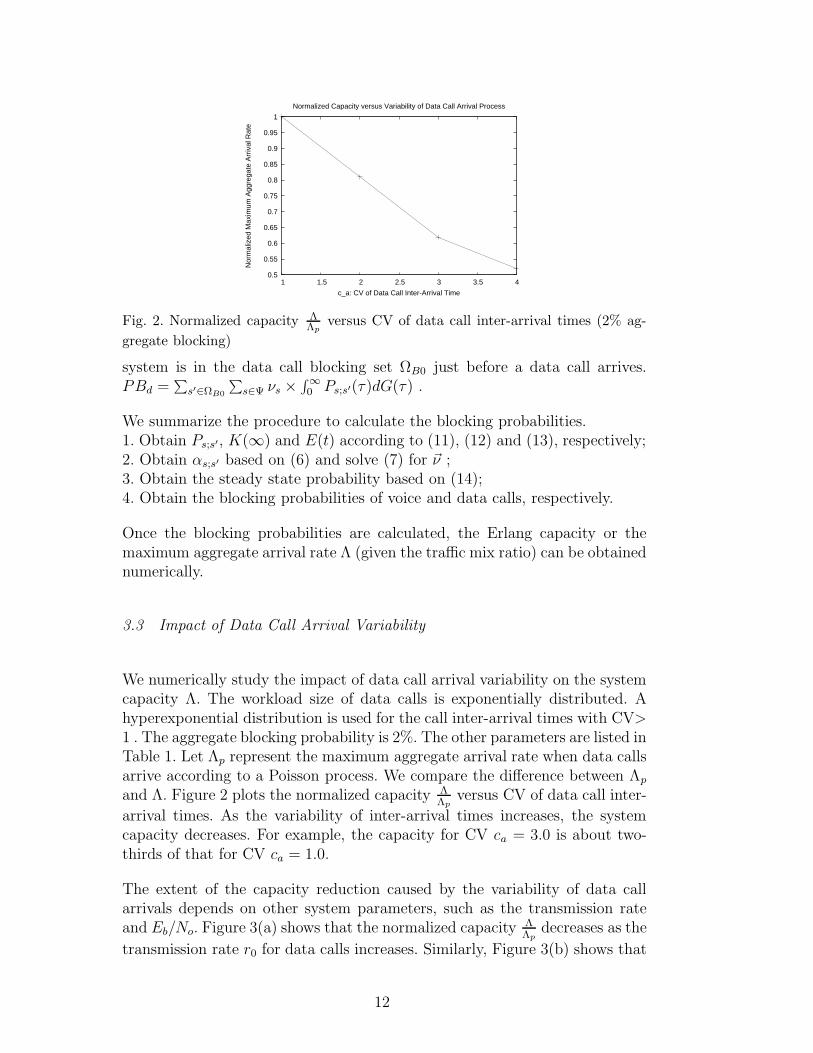
3.3 Impact of Data Call Arrival Variability

We numerically study the impact of data call arrival variability on the systemcapacity Λ. The workload size of data calls is exponentially distributed. Ahyperexponential distribution is used for the call inter-arrival times with CV>1 . The aggregate blocking probability is 2%. The other parameters are listed inTable 1. Let Λp represent the maximum aggregate arrival rate when data callsarrive according to a Poisson process. We compare the difference between Λp

and Λ. Figure 2 plots the normalized capacity ΛΛp

versus CV of data call inter-

arrival times. As the variability of inter-arrival times increases, the systemcapacity decreases. For example, the capacity for CV ca = 3.0 is about two-thirds of that for CV ca = 1.0.

The extent of the capacity reduction caused by the variability of data callarrivals depends on other system parameters, such as the transmission rateand Eb/No. Figure 3(a) shows that the normalized capacity Λ

Λpdecreases as the

transmission rate r0 for data calls increases. Similarly, Figure 3(b) shows that

12

0.4

0.5

0.6

0.7

0.8

0.9

1

0 20 40 60 80 100 120

Rel

ativ

e S

yste

m C

apac

ity

Transmission Rate r_0 per Data Call in Kbps

Relative System Capacity versus Data Call Transmission Rate

Hyperexponential(c_a = 2.0)

Hyperexponential(c_a = 3.0)

0.4

0.5

0.6

0.7

0.8

0.9

1

2 2.5 3 3.5 4 4.5 5

Rel

ativ

e S

yste

m C

apac

ity

Eb/No Requirement for Data Calls in dB

Relative System Capacity versus Eb/No for Data Call

Hyperexponential(c_a = 2.0)

Hyperexponential(c_a = 3.0)

(a) (b)

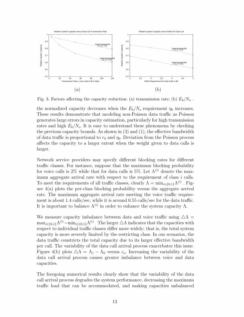
Fig. 3. Factors affecting the capacity reduction: (a) transmission rate; (b) Eb/No .

the normalized capacity decreases when the Eb/No requirement η0 increases.These results demonstrate that modeling non-Poisson data traffic as Poissongenerates large errors in capacity estimation, particularly for high transmissionrates and high Eb/No. It is easy to understand these phenomena by checkingthe previous capacity bounds. As shown in (3) and (1), the effective bandwidthof data traffic is proportional to r0 and η0. Deviation from the Poisson processaffects the capacity to a larger extent when the weight given to data calls islarger.

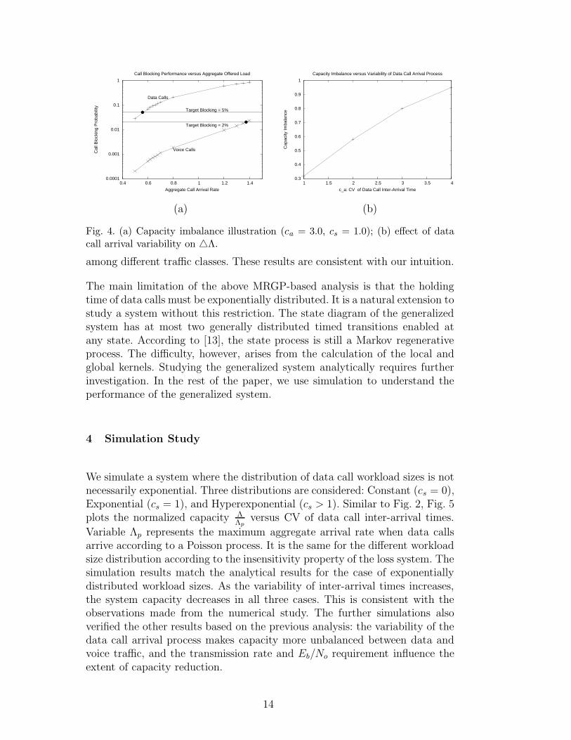
Network service providers may specify different blocking rates for differenttraffic classes. For instance, suppose that the maximum blocking probabilityfor voice calls is 2% while that for data calls is 5%. Let Λ(i) denote the max-imum aggregate arrival rate with respect to the requirement of class i calls.To meet the requirements of all traffic classes, clearly Λ = mini∈0,1Λ

(i) . Fig-ure 4(a) plots the per-class blocking probability versus the aggregate arrivalrate. The maximum aggregate arrival rate meeting the voice traffic require-ment is about 1.4 calls/sec, while it is around 0.55 calls/sec for the data traffic.It is important to balance Λ(i) in order to enhance the system capacity Λ.

We measure capacity imbalance between data and voice traffic using 4Λ =maxi∈0,1Λ

(i)−mini∈0,1Λ(i) . The larger4Λ indicates that the capacities with

respect to individual traffic classes differ more widely; that is, the total systemcapacity is more severely limited by the restricting class. In our scenarios, thedata traffic constricts the total capacity due to its larger effective bandwidthper call. The variability of the data call arrival process exacerbates this issue.Figure 4(b) plots 4Λ = Λ1 − Λ0 versus ca. Increasing the variability of thedata call arrival process causes greater imbalance between voice and datacapacities.

The foregoing numerical results clearly show that the variability of the datacall arrival process degrades the system performance, decreasing the maximumtraffic load that can be accommodated, and making capacities unbalanced

13

0.0001

0.001

0.01

0.1

1

0.4 0.6 0.8 1 1.2 1.4

Cal

l Blo

ckin

g P

roba

bilit

y

Aggregate Call Arrival Rate

Call Blocking Performance versus Aggregate Offered Load

Data Calls

Voice Calls

Target Blocking = 5%

Target Blocking = 2%

0.3

0.4

0.5

0.6

0.7

0.8

0.9

1

1 1.5 2 2.5 3 3.5 4

Cap

acity

Imba

lanc

e

c_a: CV of Data Call Inter-Arrival Time

Capacity Imbalance versus Variability of Data Call Arrival Process

(a) (b)

Fig. 4. (a) Capacity imbalance illustration (ca = 3.0, cs = 1.0); (b) effect of datacall arrival variability on 4Λ.

among different traffic classes. These results are consistent with our intuition.

The main limitation of the above MRGP-based analysis is that the holdingtime of data calls must be exponentially distributed. It is a natural extension tostudy a system without this restriction. The state diagram of the generalizedsystem has at most two generally distributed timed transitions enabled atany state. According to [13], the state process is still a Markov regenerativeprocess. The difficulty, however, arises from the calculation of the local andglobal kernels. Studying the generalized system analytically requires furtherinvestigation. In the rest of the paper, we use simulation to understand theperformance of the generalized system.

4 Simulation Study

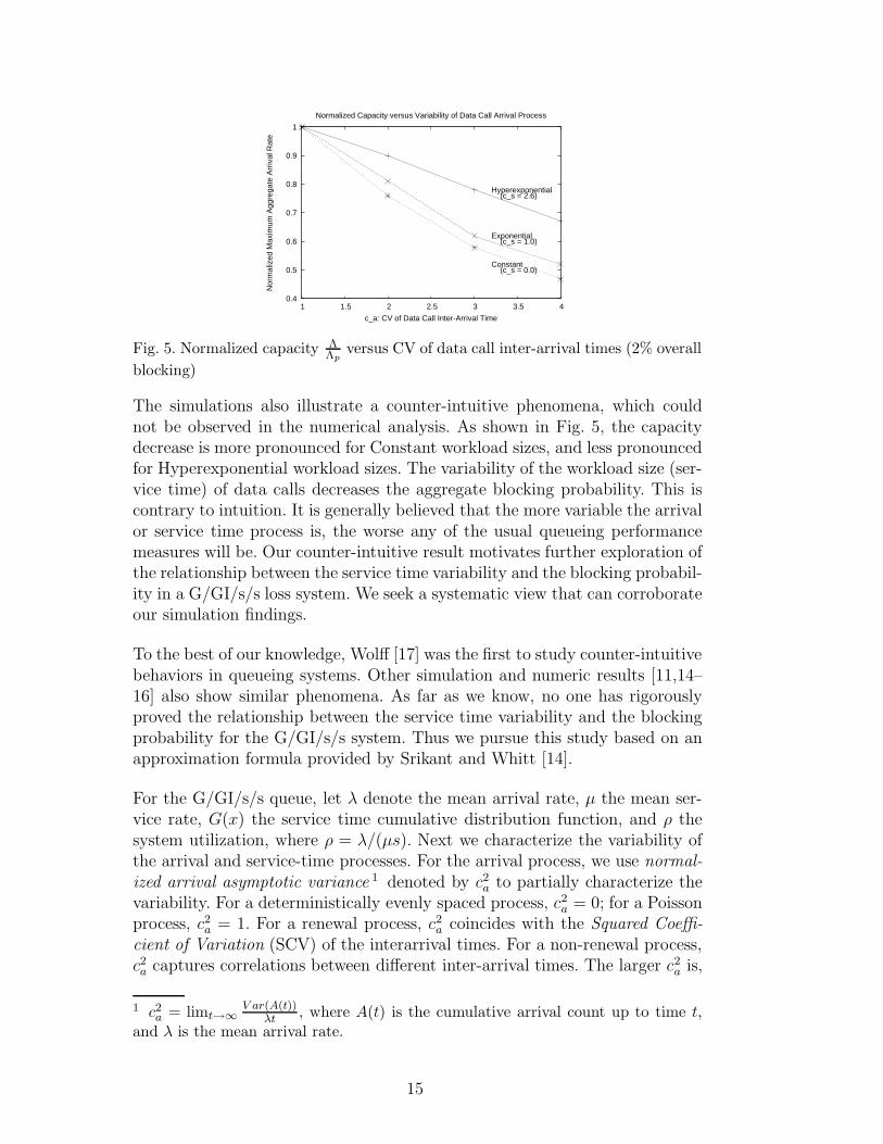
We simulate a system where the distribution of data call workload sizes is notnecessarily exponential. Three distributions are considered: Constant (cs = 0),Exponential (cs = 1), and Hyperexponential (cs > 1). Similar to Fig. 2, Fig. 5plots the normalized capacity Λ

Λpversus CV of data call inter-arrival times.

Variable Λp represents the maximum aggregate arrival rate when data callsarrive according to a Poisson process. It is the same for the different workloadsize distribution according to the insensitivity property of the loss system. Thesimulation results match the analytical results for the case of exponentiallydistributed workload sizes. As the variability of inter-arrival times increases,the system capacity decreases in all three cases. This is consistent with theobservations made from the numerical study. The further simulations alsoverified the other results based on the previous analysis: the variability of thedata call arrival process makes capacity more unbalanced between data andvoice traffic, and the transmission rate and Eb/No requirement influence theextent of capacity reduction.

14

0.4

0.5

0.6

0.7

0.8

0.9

1

1 1.5 2 2.5 3 3.5 4

Nor

mal

ized

Max

imum

Agg

rega

te A

rriv

al R

ate

c_a: CV of Data Call Inter-Arrival Time

Normalized Capacity versus Variability of Data Call Arrival Process

Constant(c_s = 0.0)

Exponential(c_s = 1.0)

Hyperexponential(c_s = 2.6)

Fig. 5. Normalized capacity ΛΛp

versus CV of data call inter-arrival times (2% overall

blocking)

The simulations also illustrate a counter-intuitive phenomena, which couldnot be observed in the numerical analysis. As shown in Fig. 5, the capacitydecrease is more pronounced for Constant workload sizes, and less pronouncedfor Hyperexponential workload sizes. The variability of the workload size (ser-vice time) of data calls decreases the aggregate blocking probability. This iscontrary to intuition. It is generally believed that the more variable the arrivalor service time process is, the worse any of the usual queueing performancemeasures will be. Our counter-intuitive result motivates further exploration ofthe relationship between the service time variability and the blocking probabil-ity in a G/GI/s/s loss system. We seek a systematic view that can corroborateour simulation findings.

To the best of our knowledge, Wolff [17] was the first to study counter-intuitivebehaviors in queueing systems. Other simulation and numeric results [11,14–16] also show similar phenomena. As far as we know, no one has rigorouslyproved the relationship between the service time variability and the blockingprobability for the G/GI/s/s system. Thus we pursue this study based on anapproximation formula provided by Srikant and Whitt [14].

For the G/GI/s/s queue, let λ denote the mean arrival rate, µ the mean ser-vice rate, G(x) the service time cumulative distribution function, and ρ thesystem utilization, where ρ = λ/(µs). Next we characterize the variability ofthe arrival and service-time processes. For the arrival process, we use normal-ized arrival asymptotic variance 1 denoted by c2

a to partially characterize thevariability. For a deterministically evenly spaced process, c2

a = 0; for a Poissonprocess, c2

a = 1. For a renewal process, c2a coincides with the Squared Coeffi-

cient of Variation (SCV) of the interarrival times. For a non-renewal process,c2a captures correlations between different inter-arrival times. The larger c2

a is,

1 c2a = limt→∞

V ar(A(t))λt , where A(t) is the cumulative arrival count up to time t,

and λ is the mean arrival rate.

15

the more variable the arrival process is. The service times are independent,and thus we use SCV (c2

s) to measure service time variability.

Since it is difficult to study the G/GI/s/s system directly, the loss systemis often associated with the G/GI/∞ model with the same arrival and ser-vice time processes. The system variability is partially characterized by thepeakedness parameter z, which is defined as the ratio of the variance to themean number of busy servers in the associated G/GI/∞. The heavy-trafficapproximation [14] for the peakedness is:

z = 1 + µ(c2a − 1)

∫ ∞

0[1−G(x)]2 dx . (15)

The value of∫∞0 [1−G(x)]2 dx decreases as the service time distribution gets

more variable.

According to [14], the blocking probability can be approximated by:

B ≈√

z

ρs

φ(−γ/√

z)

Φ(γ/√

z), (16)

where γ =√

s(1 − ρ)/√

ρ, and φ(·) and Φ(·) are the density and cumulativedistribution functions of the standard normal distribution. Formula (16) isasymptotically correct under the constraint

√s(1 − ρ)/

√ρ → γ as s → ∞ .

When this constraint is satisfied, the system must be in the heavy trafficregion. Peakedness z expressed by (15) can be used as an approximation. Thisapproximation is reasonable if z is not very large.

We combine (15) and (16) to study the qualitative behavior of the blockingprobability as a function of the service-time variability. Use ↑ for ‘increases’, ↓for ‘decreases’ and ⇒ for ‘results in’. From (15), we have: c2

s ↑⇒ z ↓, if c2a > 1;

c2s ↑⇒ z = 1, if c2

a = 1; c2s ↑⇒ z ↑, if c2

a < 1. Also from (16), we have z ↑⇒B ↑ since φ(−γ/

√z) and Φ(γ/

√z) are increasing and decreasing functions of

z, respectively. Combining the relationships among c2s, z, and B, we have:

c2s ↑⇒B ↓, if c2

a > 1, (17)

c2s ↑⇒B no change, if c2

a = 1, (18)

c2s ↑⇒B ↑, if c2

a < 1. (19)

Expression (17) is consistent with our simulations and (18) is consistent withthe insensitivity property of the M/GI/s/s system. As shown by (19), thecounter-intuitive phenomenon does not occur when the arrival process is lessvariable than a Poisson process.

This analysis corroborates our simulation results, and enhances our under-standing of the fundamental issues. It is generally believed that data traffic

16

is much variable than voice traffic. We conclude that increased variability indata call holding times decreases the blocking probability and increases theeffective system capacity.

5 Data Call Buffering

Our previous results show that increased variability in the data call arrival pro-cess reduces the system capacity and exacerbates capacity imbalance amongtraffic classes. These observations motivate a simple buffer-based resourcemanagement scheme for data calls. The rationale for the data call buffer-ing scheme is three-fold. First, data traffic is generally more tolerant to delaythan voice traffic. Second, buffering can effectively mitigate the variability inthe data call arrival process. Third, buffering data calls temporarily ratherthan immediately blocking them provides these calls a better opportunity toenter the system later. In other words, buffering can provide a controllableperformance tradeoff between voice and data calls.

The buffering scheme works as follows. Arriving data calls that encounter afull system must enter a FIFO queue. The buffer size is infinite, so no datacall is blocked due to insufficient buffer space. Each of the buffered calls hasan associated timer set to a maximum delay tB. The timer starts when thecall enters the queue. When a call releases a channel from the system, thesystem checks whether it has room for buffered data calls. If there are M2

data calls in the buffer, and there is room for M1 calls, then min(M1, M2)data calls are removed from the buffer to access channels. Otherwise, no datacall is accepted at that moment. A call is cleared from the buffer once itstimer expires. Thus, data call blocking can occur tB seconds after arriving.Furthermore, only unexpired data calls can access channels. For voice calls,the system works as an ordinary loss system. If there are available resourcesat the time of arrival, the call is accepted. Otherwise, the call is blocked rightaway. Voice calls have priority over buffered data calls to access channels.

Buffering reduces the aggregate blocking rate by slightly increasing the datacall delay. We measure its efficiency by the relative capacity increase Λ(b)−Λ

Λ,

where Λ(b) is the maximum aggregate arrival rate when data call buffering isapplied. Simulation is employed to study the impact of the stochastic proper-ties of data calls on the efficiency of the buffering strategy.

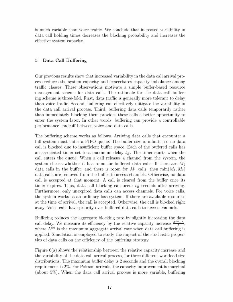
Figure 6(a) shows the relationship between the relative capacity increase andthe variability of the data call arrival process, for three different workload sizedistributions. The maximum buffer delay is 2 seconds and the overall blockingrequirement is 2%. For Poisson arrivals, the capacity improvement is marginal(about 5%). When the data call arrival process is more variable, buffering

17

0

0.05

0.1

0.15

0.2

0.25

0.3

1 1.5 2 2.5 3 3.5 4

Rel

ativ

e C

apac

ity In

crea

se

c_a: CV of Data Call Inter-Arrival Time

Relative Capacity Increase versus Variability of Data Call Arrival Process

Constant(c_s = 0)

Exponential(c_s = 1)

Hyperexponential(c_s = 2.6)

0

0.2

0.4

0.6

0.8

1

1 1.5 2 2.5 3 3.5 4

Cap

acity

Imba

lanc

e

c_a: CV of Data Call Inter-Arrival Time

Capacity Imbalance versus Variability of Data Call Arrival Process

No Buffering

Buffering

Constant

Exponential

Constant

Exponential

(a) (b)

Fig. 6. Effect of data call buffering (2s maximum delay) on (a) relative capacity

increase Λ(b)−ΛΛ ; (b) capacity imbalance ∆Λ = Λ1 − Λ0 .

offers capacity improvements of 10-25%. The greatest capacity improvementis observed for the Constant workload size distribution.

The buffering scheme also provides control over the tradeoff between block-ing rates for different traffic classes. In our earlier results, capacity imbalancebetween voice and data traffic is inherent due to the higher effective band-width of data calls. This imbalance is further aggravated by data call arrivalvariability. However, the buffering scheme gives data calls more chances to en-ter the system. The blocking probability of data traffic is thus reduced, whilethat of voice traffic increases. As a result, this scheme balances the capacityrestrictions from different traffic class requirements. Figure 6(b) compares thecapacity imbalance, ∆Λ, for cases with and without buffering. In all cases,buffering mitigates the capacity imbalance between data and voice traffic, andthus enhances the overall capacity of the CDMA system.

In Section 4, we observed a counter-intuitive phenomenon with respect tothe variability of data call workload sizes. The phenomenon still exists whendata call buffering is applied. However, this effect is less pronounced when themaximum buffer delay increases.

Though simple, the data call buffering scheme can effectively enhance thesystem capacity when the data traffic arrival process is highly variable. Ad-justing the maximum buffer delay provides controllable performance tradeoffsbetween blocking probability and delay, and between voice and data traffic.

6 Conclusions

This paper studies a multi-service CDMA system supporting voice and datatraffic. The main emphasis in our work is on understanding the impacts of

18

non-Poisson data traffic on overall CDMA system capacity.

We first study the system based on a Markov Regenerative Process (MRGP)model, and then explore a more general system using simulation. Our resultsshow that increased variability in the data call arrival process decreases thesystem capacity, while increased variability in data call holding times increasesthe capacity. The extent of the phenomena observed depends on other systemparameters, such as transmission rates and Eb/No requirements. We also studya buffer-based resource management scheme that enhances the system capacityin the presence of high-variability data traffic.

Ongoing work is exploring the impact of correlated data call interarrival timesand workload sizes on the capacity. We also plan to investigate the capacityof the CDMA2000-1xEVDO system using more realistic traffic models.

References

[1] E. Altman, “Capacity of Multi-service Cellular Networks with TransmissionRate Control: A Queueing Analysis”, Proceedings of ACM MOBICOM, Atlanta,GA, pp. 205-214, September 2002.

[2] X. Bo and Z. Chen, “On Call Admission and Performance Evaluation forMultiservice CDMA Networks”, ACM SIGMOBILE Mobile Computing andCommunications Review, Vol. 8, No. 1, pp. 98-108, 2004.

[3] S. Dharmaraja, D. Logothetis, and K. Trivedi, “Performance Modelling ofWireless Networks with Generally Distributed Handoff Interarrival Times”,Computer Communications, Vol. 26, pp. 1747-1755, 2003.

[4] R. German, Performance Analysis of Communication Systems: Modeling withNon-Markovian Stochastic Petri Nets, Wiley, 2000.

[5] N. Hegde and E. Altman, “Capacity of Multiservice WCDMA Networks withVariable GoS”, IEEE Wireless Communications and Networking Conference,Vol. 4, No. 1, pp. 1402-1407, March 2003.

[6] Y. Ishikawa and N. Umeda, “Capacity Design and Performance of CallAdmission Control in Cellular CDMA Systems”, IEEE Journal on SelectedAreas in Communications, Vol. 15, No. 8, pp. 1627-1635, 1997.

[7] W. Jeon and D. Jeong, “Call Admission Controlfor CDMA Mobile Communications Systems Supporting Multimedia Services”,IEEE Transactions on Wireless Communications, Vol. 1, No. 4, pp. 649-659,October 2002.

[8] I. Koo, J. Ahn, J. Lee, and K. Kim, “Analysis of Erlang Capacity forthe Multimedia DS-CDMA Systems”, IEICE Transactions on Fundamentals,Vol. E82-A, No. 5, pp. 849-855, 1999.

19

[9] V. Kulkarni, Modeling and Analysis of Stochastic Systems, Chapman & Hall,London, 1995.

[10] J. Lee and L. Miller, “Solutions for Minimum Required Forward Link ChannelPower in CDMA Cellular and PCS Systems”, Journal of Communications andNetworks, Vol. 1, No. 1, pp. 42-51, March 1999.

[11] H. Masuyama and T. Takine, “Analysis of an Infinite-Server Queue with BatchMarkovian Arrival Streams”, Queueing Systems, Vol. 42, No. 3, pp. 269-296,2002.

[12] V. Paxson and S. Floyd, “Wide Area Traffic: The Failure of Poisson Modeling”,IEEE/ACM Transactions on Networking, Vol. 3, No. 3, pp. 226-244, 1994.

[13] A. Puliafito, M. Scarpa, and K. Trivedi, “Petri Nets with k SimultaneouslyEnabled Generally Distributed Timed Transitions”, Performance Evaluation,Vol. 32, No. 1, pp. 1-34, 1998.

[14] R. Srikant and W. Whitt, “Simulation Run Lengths to Estimate BlockingProbabilities”, ACM Transactions on Modeling and Computer Simulation,Vol. 6, pp. 7-52, January 1996.

[15] W. Whitt, “Heavy Traffic Approximations for Service Systems with Blocking”,Bell Labs Technical Journal, Vol. 63, pp. 689–708, 1984.

[16] W. Whitt, “A Diffusion Approximation for the G/GI/n/m Queue”, OperationResearch, Vol. 52, No. 6, pp. 922-941, November/December 2004.

[17] R. Wolff, “The Effect of Service Time Regularity on System Performance”,Computer Performance (edited by K. Chandy and M. Reiser), pp. 297-304,North-Holland, 1977.

Yujing Wu received the Ph.D. degree in Electrical and Computer Engineeringfrom the University of Massachusetts at Amherst. She is a postdoctoral fellowin the Department of Computer Science at the University of Calgary, whereshe does research on capacity planning of 3G cellular networks.

Carey Williamson is an iCORE Professor in the Department of ComputerScience at the University of Calgary, specializing in Wireless Internet TrafficModeling. He holds a B.Sc.(Honours) in Computer Science from the Universityof Saskatchewan, and a Ph.D. in Computer Science from Stanford University.His research interests include Internet protocols, wireless networks, networktraffic measurement, network simulation, and Web server performance.

20