Embed Size (px)
Citation preview
Derived categories. Winter 2008/09
Igor V. Dolgachev
May 5, 2009

ii
Contents
1 Derived categories 11.1 Abelian categories . . . . . . . . . . . . . . . . . . . . . . . . . . 11.2 Derived categories . . . . . . . . . . . . . . . . . . . . . . . . . . 91.3 Derived functors . . . . . . . . . . . . . . . . . . . . . . . . . . . 241.4 Spectral sequences . . . . . . . . . . . . . . . . . . . . . . . . . . 381.5 Exercises . . . . . . . . . . . . . . . . . . . . . . . . . . . . . . . 44
2 Derived McKay correspondence 472.1 Derived category of coherent sheaves . . . . . . . . . . . . . . . . 472.2 Fourier-Mukai Transform . . . . . . . . . . . . . . . . . . . . . . 592.3 Equivariant derived categories . . . . . . . . . . . . . . . . . . . . 752.4 The Bridgeland-King-Reid Theorem . . . . . . . . . . . . . . . . 862.5 Exercises . . . . . . . . . . . . . . . . . . . . . . . . . . . . . . . 100
3 Reconstruction Theorems 1053.1 Bondal-Orlov Theorem . . . . . . . . . . . . . . . . . . . . . . . . 1053.2 Spherical objects . . . . . . . . . . . . . . . . . . . . . . . . . . . 1133.3 Semi-orthogonal decomposition . . . . . . . . . . . . . . . . . . . 1213.4 Tilting objects . . . . . . . . . . . . . . . . . . . . . . . . . . . . 1283.5 Exercises . . . . . . . . . . . . . . . . . . . . . . . . . . . . . . . 131
iii

iv CONTENTS
Lecture 1
Derived categories
1.1 Abelian categories
We assume that the reader is familiar with the concepts of categories and func-tors. We will assume that all categories are small , i.e. the class of objects Ob(C)in a category C is a set. A small category can be defined by two sets Mor(C) andOb(C) together with two maps s, t : Mor(C)→ Ob(C) defined by the source andthe target of a morphism. There is a section e : Ob(C)→ Mor(C) for both mapsdefined by the identity morphism. We identify Ob(C) with its image under e.The composition of morphisms is a map c : Mor(C) ×s,t Mor(C) → Mor(C).There are obvious properties of the maps (s, t, e, c) expressing the axioms ofassociativity and the identity of a category. For any A,B ∈ Ob(C) we denoteby MorC(A,B) the subset s−1(A) ∩ t−1(B) and we denote by idA the elemente(A) ∈ MorC(A,A).
A functor from a category C defined by (Ob(C),Mor(C), s, t, c, e) to a cate-gory C′ defined by (Ob(C′),Mor(C′), s′, t′, c′, e′) is a map of sets F : Mor(C)→Mor(C′) which is compatible with the maps (s, t, c, e) and (s′, t′, c′, e′) in theobvious way. In particular, it defines a map Ob(C) → Ob(C ′) which we alsodenote by F .
For any category C we denote by Cop the dual category , i.e. the category(Mor(C),Ob(C), s′, t′, c, e), where s′ = t, t′ = s. A contravariant functor fromC to C′ is a functor from Cop to C. For any two categories C and D we denoteby DC (or by Funct(C,D)) the category of functors from C to D. Its set ofobjects are functors F : C → D. Its set of morphisms with source F1 andtarget F2 are natural transformation of functors, i.e. maps Φ = (Φ1,Φ2) :Mor(C) → Mor(D) × Mor(D) such that (s × t) Φ = (s × t) (F1, F2) and(t × s) Φ = (t × s) (F1, F2), and Φ2 F1 = F2 Φ1. It is also required thatΦi(u v) = Φi(u) Φi(v) and Φi(idA) = idFi(A), for any A ∈ Ob(C).
Let Sets be the category of small sets (i.e. subset of some set which wecan always enlarge if needed). We denote by C the category SetsC
op. A typical
example is when we take C = Open(X) to be the category of open subsets of
1
2 LECTURE 1. DERIVED CATEGORIES
a topological space X with inclusions as morphisms, a contravariant functorF : Open(X) → Sets is a presheaf on X. For this reason, the objects of C arecalled presheaves on C.
Any A ∈ Ob(C) defines the presheaf
hA : (φ : X → Y )→ (MorC(Y,A)φ−→ MorC(X,A))
For any morphism u : A → A′ in C and any A ∈ Ob(C), composing on the leftdefines a map hA(A)→ hA′(A), and the set of such maps makes a morphism offunctors hA → hA′ . This defines a functor
h : C→ C, MorC(A,A′)→ MorbC(hA, hA′)
called the Yoneda functor or the representation functor . According to theYoneda lemma this functor is fully faithful , i.e. defines a bijection
MorC(A,A′)→ MorbC(hA, hA′).
Via the Yoneda functor, the category C becomes equivalent to a full subcategoryof the category C (a subcategory C′ is full if MorC′(A,B) = MorC(A,B)). Alsorecall that a category C′ is equivalent to a category C if there exist functorsF : C′ → C, G : C→ C′ such that the compositions F G,G F are isomorphic(in the category of functors) to the identity functors. A presheaf F ∈ C iscalled representable if it is isomorphic to a functor of the form hS for someS ∈ C. We say that F and G are quasi-inverse functors. The object S iscalled the representing object of F . It is defined uniquely, up to isomorphism.Dually, one defines the functor hA : C → Sets whose value at an object X isequal to MorC(A,X). A functor C→ Sets isomorphic to a functor hA is calledcorepresentable.
Let S be a subcategory of the category Sets. A category C is called an S-category if for any X ∈ Ob(C) the presheaf hX takes values in S and for any(A → B) ∈ Mor(C), the map hX(A) → hXB) is a morphism in S. We willbe interested in the case when S = Ab is the category of abelian groups. Inthis case an Ab-category is called a Z-category . It follows from the definitionthat the sets of morphisms is equipped with a structure of an abelian group,moreover, the left composition map MorC(A,B) → MorC(A,C) and the rightcomposition map MorC(B,C)→ MorC(A,C) are homomorphisms of groups.
Another useful example is when A is the category of linear spaces over afield K. This allows to equip the sets of morphism with compatible structuresof linear spaces. In this case a category is called K-linear .
From now on, whenever we deal with a Z-category category we set HomC(A,B) :=MorC(A,B).
Let Cab
be the category of abelian presheaves on C, i.e. the category ofcontravariant functors from C to Ab. If C is a Z-category, the Yoneda functoris the functor from C to C
ab. For any abelian group A one defines the constant
presheaf AC (or just A if no confusion arises) by
AC(S) = A, (S → S′)→ idA.
1.1. ABELIAN CATEGORIES 3
In particular, we have the zero presheaf 0. For any F ∈ Cab
, we have HombCab(0, F ) =0 and the zero represents the unique morphism 0→ F .
A zero object of a Z-category is an object representing the functor 0. It maynot exist, but when they exist all of them are isomorphic and can be identifiedwith one object denoted by 0. The zero object 0 is characterized by the propertythat HomC(0, 0) = 0. This immediately implies that 0 is the initial and thefinal object in C, i.e., for any X ∈ Ob(C) there exists a unique morphism0 → X (resp. X → 0). It represents the zero element in HomC(0, X) (resp. inHomC(X, 0)).
For any morphism u : F → G of abelian presheaves we can define the kernelker(u) by
ker(u)(A) = ker(F (A)→ G(A)).
It can be characterized by the following universal property: there is a morphismker(u)→ F such that the composition ker(u)→ F → G is the zero morphism,and any morphism K → F with this property factors through the morphismker(u)→ F . We say that C has kernels if, for any X → Y the kernel of hX → hY
in Cab
is representable. By the Yoneda Lemma, the kernel ker(X → Y ) satisfiesthe universal property from above, and this can be taken as the equivalentdefinition.
The definition of the cokernel coker(u) of a morphism X → Y in a pre-additive category is obtained by reversing the arrows. It comes with a uniquemorphism Y → coker(u) such that any morphism Y → K with the zero com-position F → G→ K factors through G→ coker(u)→ K. In other words,
coker(u) = ker(uop)op,
where uop : G → F is a morphism in the dual category Cop and ker(uop)op isthe morphism ker(u0) → G in Cop considered as a morphism G → ker(uop) inC.
Note that Cab
has cokernels defined by
coker(F → G)(S) = coker(F (S)→ G(S)).
However, even when C = Ab where kernels and cokernels are the usual ones,coker(hA → hB) may not be representable. For example, if we take [n] : Z→ Zthe multiplication by n > 1 in Ab and u = h([n]) : hZ → hZ, then we get
coker(u)(Z/nZ) = coker(hZ(Z/nZ)→ hZ(Z/nZ)) = coker(0→ 0) = 0,
because Hom(Z/nZ,Z) = 0. On the other hand,
hcoker([n])(Z/nZ) = hZ/nZ(Z/nZ) = Hom(Z/nZ,Z/nZ) 6= 0.
It follows from the definition that there is a canonical morphism
coker(ker(u)→ s(u)) α→ ker(t(u)→ coker(u)), (1.1)

4 LECTURE 1. DERIVED CATEGORIES
where u : s(u)→ t(u) is a morphism in C (provided that all the objects in aboveexist). The morphism u factors as
s(u)→ coker(ker(u)→ s(u))→ ker(t(u)→ coker(u))→ t(u).
The category Cab
contains finite direct products over the final object 0 de-fined by the standard universality property. We have
(∏i∈I
Fi)(A) ∼=∏i∈I
Fi(A).
It also contains finite direct sums ⊕i∈IFi over the initial object 0C, defined asthe direct product in the dual category. Moreover,∏
i∈IFi ∼=
⊕i∈I
Fi.
It follows from the Yoneda Lemma that the object representing the direct prod-ucts (sums) of representable presheaves is the direct product (sum) of the rep-resenting objects.
Definition 1.1.1. An additive category is a Z-category such that
(i) the zero presheaf 0 is representable;
(ii) finite direct sums and direct products in Cab
are representable;
An additive category is called abelian if additionally
(iii) kernels and cokernels exist;
(iv) for any morphism u,
coker(ker(u)→ s(u)) = ker(t(u)→ coker(u)),
and the canonical morphism α in (1.1) is an isomorphism. The objectcoker(ker(u) → s(u)) is denoted by im(u) and is called the image of themorphism u.
Recall that a morphism u : s(u) → t(u) is called a monomorphism if thecorresponding morphism h(u) : hs(u) → ht(u) in C is injective on its values. Inother words, for any S ∈ Ob(C) the map of sets hs(u)(S) = MorC(S, s(u)) u−→MorC(S, t(u)) is injective. By reversing the arrows one defines the notion of anepimorphism. If C is an abelian category, then u is a monomorphism (resp.epimorphism) if and only if ker(u) = 0 (resp. coker(u) = 0). Also u is anisomorphism (i.e. the left and the right inverses exist) if and only if it is amonomorphism and an epimorphism.
In an abelian category short exact sequences make sense. Also one can definethe cochain complexes as sequences K• = (un : Kn → Kn+1)n∈I of morphisms
1.1. ABELIAN CATEGORIES 5
with un+1 un = 0 ∈ HomC(Kn,Kn+2). Here n runs an interval I (finite orinfinite) in the set of integers. Also one can define the cohomology of complexesas the complex
(Hn(K•), 0) = coker(im(un)→ ker(un+1))
with the zero morphisms Hn → Hn+1. By reversing the arrows one defineschain complexes and the notion of homology of a complex K• = (un : Kn →Kn−1)n∈I .
Finally, let us give some examples of abelian categories. Of course the firstexample must be the category Ab of abelian groups, it is the motiviating exampleof the whole theory. If A is an abelian category, then the category ACop
of A-valued presheaves on C is an abelian category. In particular, the category C
ab
is an abelian category.Let Shab
X be the category of abelian sheaves on a topological space (or ona Grothendieck topology) considered as a full subcategory of the category of
abelian presheaves PShabX = C
ab. It is not a trivial fact that it is an abelian
category. One uses the fact that the forgetting functor ι : ShabX → PShab
X admitsthe left inverse functor as : PShab
X → ShabX (i.e. asι is isomorphic to the identity
functor in ShabX ). The functor as is defined by the standard construction of the
sheafication F# of a presheaf F . For any morphism u : F → G of abeliansheaves one has
ker(u) = ker(ι(u)))#, coker(u) = coker(ι(u))#
(in fact, ι(ker(u)) = ker(ι(u))).Another example is the category Mod(R) of (left) modules over a ring R
(all rings will be assumed to be associative and contain 1). It is consideredas a subcategory of Ab. The kernels and cokernels in Ab of a morphism inMod(R) can be equipped naturally with a stricture of R-modules and representthe kernels and cokernels in Mod(R).
A generalization of this example is the category of sheaves of modules over aringed space (X,OX). The most important for us example will be the categoryQcoh(X) of qusi-coherent sheaves and its full subcategory CohX of coherentsheaves on a scheme X.
Another frequently used example of an abelian category is the category ofquivers with values in an abelian category A (or the category of diagrams in Aas defined by Grothendieck). We fix any oriented graph Γ and assign to eachits vertex v an object X(v) from A. To each arrow a with tail t(a) and headh(a) we assign a morphism from u(a) : X(t(a))→ X(h(a)) in A.
A morphism of diagrams (X(v), u(a))→ (X ′(v), u′(a)) is a set of morphismsφv : X(v)→ X ′(v) such that, for any arrow a the diagram
X(t(a))φt(a) //
u(a)
X ′(t(a))
u′(a)
X(h(a))
φh(a) // X ′(h(a))
6 LECTURE 1. DERIVED CATEGORIES
is commutative.One can consider different natural subcategories of the category Diag(Γ,A)
of the category of diagrams in A with fixed graph Γ. A diagram is calledcommutative if for any path p = (a1, . . . , ak) the composition u(p) = u(a1) · · · u(ak) depends only on t(p) := t(ak) and h(p) := h(a1). It is easy tocheck that commutative diagrams form an abelian subcategory of the categoryof diagrams. A commutative diagram is called a diagram complex if for any pathdifferent from an arrow, the morphism u(p) is the zero morphism. A complex inA defined in above corresponds to a linear graph. All diagram complexes forman abelian subcategory of the category Diag(Γ,A). In particular, the categoryof cochain complexes in an abelian category is an abelian category.
Here are some examples of additive but not abelian categories. Obviouslyan additive subcategory of an abelian category is not abelian in general. Forexample, the category of projective modules over a ring R is additive but hasno kernels or cokernels for some homomorphisms of projective R-modules. Anadditive subcategory may have kernels or cokernels but (1.1) may not be an iso-morphism. The most notorious example is the category of filtered abelian groupsA = ∪i∈NA
i, Ai ⊂ Ai+1 with morphisms compatible with filtrations. Changingthe filtration by ′Ai := Ai+1 and considering the identity morphism we obtaina non-invertible morphism that is an monomorphism and an epimorphism.
Let us consider the category Mod(R) of left modules over a ring R. Notethat the category of right R-modules is the category Mod(Rop), where Rop isthe opposite ring. The category Mod(R) is obviously an abelian category. Itsatisfies the following properties
(i) For each set (Mi)i∈I of objects in Mod(R) indexed by any set of I thereexists the direct sum ⊕i∈IMi. It corepresents the functor
∏i∈I h
Mi .
(ii) The ring R considered as a module over itself is a generator P of Mod(R)(i.e. any object M admits an epimorphism RI →M for some set I, whereRI denotes the direct sum ⊕i∈IRi of objects Ri isomorphic to R).
(iii) the generator P is a projective object (i.e. the functor M → HomA(R,M)sends epimorphisms to epimorphisms;
(iv) the functor hP commutes with arbitrary set-indexed direct sums.
Theorem 1.1.1. Let A be an abelian category satisfying the conditions (i) −(iv) from above where Mod(R) is replaced with A. Then A is equivalent to thecategory Mod(R), where R = End(P ) := HomA(P, P )
Proof. For any ring R we define the new category Mod(R,A). Its objects arehomomorphisms of rings φ : R→ EndA(X), X ∈ Ob(A). The set of morphismsfrom φ : R → End(X) to ψ : R → End(Y ) is the subset of morphisms f ∈HomA(X,Y ) such that ψ(r) f = f φ(r) for any r ∈ R. It is easy to checkthat Mod(R,A) is an abelian category. For example, if f ∈ HomA(X,Y ) is amorphism in Mod(R,A), then its kernel consists of homomorphisms from R toEnd(ker(f)). Obviously Mod(R,Ab) ≈ Mod(R).
1.1. ABELIAN CATEGORIES 7
Let R = EndA(U)op, where U is a fixed object of A. The composition ofmorphisms defines a map
R×HomA(U,X)→ HomA(U,X).
It is easy to see that it equips the abelian group hU (X) = HomA(U,X) with astructure of a R-module. Also it is easy to check that hU : A → Sets factorsthrough the subcategory Mod(R) of Sets, i.e. defines a functor
S = hU : A→ Mod(R).
For any Rop-module M , any X ∈ Ob(Mod(R,A)) and any Y ∈ Ob(A) we canconsider the set HomRop(M,hX(Y )). The assignment Y → HomRop(M,hX(Y ))is a presheaf on Aop with values in the category of Rop-modules. When it isrepresentable, a representing object is denoted by M⊗RX. Replacing R by Rop
we have the notation X ⊗RM , where M is a R-module, and X ∈ Mod(Rop,A).This agrees with the usual notation of the tensor product A ⊗R B of a rightR-module A and a left R-module B.
Now we assume that U is a projective generator of A. Let us consider U as anobject of Mod(Rop) defined by the identity homomorphism Rop → EndA(U).One proves that under the conditions of the theorem, U ⊗R M exists. Todo so we first consider the case M = R, where we get a natural bijectionHomRop(R, hU (Y )) → HomA(U, Y ). Then we consider the case when M = RI
by considering the bijection HomRop(RI , hU (Y )) → HomA(U I , Y ). Finally, ifM = coker(RJ → RI) we take U ⊗M to be the cokernel of UJ → U I .
We choose a representing object and denote it by U ⊗R M . Now we candefine a functor
T : Mod(R)→ A, M → U ⊗RM.
By definition, for any A ∈ Ob(A) and any M ∈ Mod(R), there is a naturalbijection
HomR(M,S(A)) = HomR(M,HomA(U,N))→ HomA(T (M), A).
In particular, the functor T is the left adjoint functor to the functor S. Recallthat a functor G : C′ → C is called a left adjoint functor to the functor F : C→C′ (and F is the right adjoint to G) if there is an isomorphism of bifunctors onC× C′op defined by
(X,Y )→ MorC(G(X), Y ), (X,Y )→ MorC′(X,F (Y )).
I leave to the reader to define the product of two categories and a bifunctordefined on the product. By taking Y = G(X), the image of the identity idYdefines a morphism X → F G(X). All such morphisms define a morphism offunctors idC′ → F G. Similarly we define a morphism of functors GF → idC.Conversely, a pair of morphisms of functors
α : idC′ → F G, β : G F → idC
8 LECTURE 1. DERIVED CATEGORIES
satisfying the property that the compositions
GGα−→ G F G βG−→ G, F
αF−→ F G F Fβ−→ F
are the identity morphisms of the functors make G left adjoint to F . In partic-ular, an equivalence of categories is defined by a pair of adjoint functors.
Note that a pair (G,F ) of adjoint functors, in general, do not define anequivalence of categories, i.e. neither α : G F → idC nor β : idC′ → F G isan equivalence of categories. However, if F is an equivalence of categories thenany quasi-inverse functor to F is a left and a right adjoint functor.
An example of a pair of adjoint functors is (G,F ) = (f∗, f∗), where f : X →Y is a morphism of schemes and (C,C′) = (Qcoh(Y ),Qcoh(X)), the categoriesof quasicoherent sheaves. Another example is the functor
HomR(B, ?) : Mod(S)→ Mod(R), N → HomS(B,N)
and its left adjoint functor
?⊗R B : Mod(R)→ Mod(S), M →M ⊗R B,
where R,S are rings and B is a (R − S)-bimodule (i.e. a left R-module and aright S-module).
Recall that a functor F : C → C′ is called left exact (resp. right exact) ifit transforms monomorphisms (resp. epimorphisms) to monomorphisms (resp.epimorphimsm). It is called exact if is left and right exact. Suppose F ad-mits a left adjoint functor G. Then F is left exact and G is right exact.Let us see it in the case of functors of abelian categories. It is enough toshow that F transforms kernels to kernels. Let K = ker(u : X → Y ) andY → ker(F (X) → F (Y ) be a morphism in A′. Applying G we get a mor-phism G(Y ) → ker(G(F (X)), G(F (Y ))). Composing G(Y ) → G(F (X)) withG(F (X)) → X we get a morphism G(Y ) → X which as is easy to see factorsthrough G(Y )→ ker(X → Y ). This shows that there is a morphism G(Y )→ Kand applying F we get a morphism Y → F (G(Y )) → F (K). This shows thatF (K) is the kernel of F (u).
Since T is the left adjoint of S, we obtain that S is left exact. Since U is aprojective object in A, we obtain that S is right exact, hence exact , i.e. left andright exact. Condition (iv) implies that S(U I) = S(U)I . It is easy to see that
HomA(U I , U j) =∏i
⊕j∈IHomC(Ui, Uj) =∏i∈I⊕j∈IHomR(S(Ui),S(Uj))
= HomR(⊕i∈IS(Ui),⊕j∈IS(Uj)) = Hom(R,S(⊕i∈IUi),⊕j∈IF (Uj))).
This shows that S defines an equivalence from the subcategory of A formed byobjects isomorphic to direct sums U I and the subcategory of Mod(R) formedby free modules. Since U and R are projective generators this easily allows toextend the equivalence to an equivalence between the categories A and Mod(R).
1.2. DERIVED CATEGORIES 9
Example 1.1.2. Let A = PShab(X) be the category of abelian presheaves ona topological space X. For any open subset V denote by ZV the sheaf equalto the constant sheaf Z on V and zero outside U . Then ⊕V ∈Ob(Open(X))ZV isa generator of A. The generator U is not projective, however if we pass to thecategory of sheaves and replace U with the associated sheaf U# we obtain aprojective generator.
More generally, consider the category of abelian presheaves Cab
on a categoryC. Then U = ⊕X∈Ob(C)ZhX is a generator of this category.
Definition 1.1.2. An abelian category satisfying properties from the assertionof the previous theorem is called a Grothendieck category.
Corollary 1.1.3. For any abelian category A there exists a fully faithful additiveexact functor to a a category Mod(R) (an additive functor of abelian categoriesis a functor which is a functor of the corresponding abelian presheaves).
Proof. It is enough to construct such a functor with values in a Grothendieckcategory. We first embed A in the category of abelian presheaves A
ab. Then
we consider a canonical Grothendieck topology on A where all representablepresheaves become automatically sheaves. We take B be the category of sheaveson A with respect to the canonical topology. The product of representablesheaves will serve as a projective generator. The Yoneda functor h : A → Bwill be an additive fully faithful exact functor. Then we apply the previoustheorem.
Suppose F : Mod(R) → A is an equivalence of abelian categories. ThenU = F (R) is a projective generator of A and R ∼= End(U). For example,we may take A = Mod(S) for some other ring S. Then Mod(R) ≈ Mod(S)implies that there exists a projective S-module U generating Mod(S) such thatEnd(S) ∼= R. In fact, the proof of the previous theorem shows that U has astructure of S −R-bimodule and the equivalence of categories is defined by thefunctor M →M ⊗S U . Two rings are called Morita equivalent if the categoriesMod(R) and Mod(S) are equivalent. A good example is the equivalence betweenthe category Mod(R) and the category Mod(S), where S = End(Rn).
1.2 Derived categories
Let Cp(A) denote the category of cochain complexes K• = (Kn, dnK)n∈Z in anabelian category A. We can always assume that the interval parametrizing Kn
is the whole Z by adding the zero objects and the zero differentials.
We shall denote by Cp(A)+ (resp. Cp(A)−) the full subcategory formed bycomplexes such that there exists N such that Ki = 0 for i < N (resp. Ki = 0for i > N). They are called bounded from below (resp. from above). A boundedcomplex is a complex bounded from below and from above. The category of
10 LECTURE 1. DERIVED CATEGORIES
those is denoted by Cpb(A). The category Cp(A) comes with the shift functorT : Cp(A)→ Cp(A), defined by T (K•) = K•[1], where
K•[1]n = Kn+1, dnT (K•) = −dn+1K .
We set K•[n] = Tn(K•), where Tn denotes the composition of functors. Notethat T has the obvious inverse, so we may define K[n] for any integer n. Bydefinition,
diK•[n] = (−1)ndi+nK• .
The differentials (dnK) define a morphism d : K → K[1] such that the composi-tion T (d) d : K → K[1]→ K[2] is the zero morphism.
Recall that a simplicial complex is a presheaf on the category whose ob-jects are natural numbers and morphisms are non-decreasing maps of intervals
f : [0, n] → [0,m]. A simplicial complex X = (XmX(f)−→ Xn)n≤m defines a
topological space |X| called the geometric realization. One considers the sets
∆n = (x0, . . . , xn) ∈ Rn+1 : x0 + . . .+ xn = 1, xi ≥ 0,
and let
|X| =∞∐n=0
∆n ×Xn/R,
where R is the minimal equivalence relation which identifies the points (s, x) ∈∆n×Xn and (t, y) ∈ ∆m×Xm if y = X(f)(x), s = ∆(f)(t) for some morphismf : m → n. Here ∆(f) is the unique affine map that sends the vertex eito the vertex ef(i). The topology is the factor-topology. For example, ∆n
is homeomorphic to the topological realization of the simplicial complex h[n]
whose value on [m] is equal to the set of non-decreasing maps [m]→ [n].A topological space is called triangulazable if it is homeomorphic to |X| for
some simplicial set X. A chosen homeomorphism is called a triangulation. LetCn(X) = ZXn and let ιin : [n − 1] → [n] whose image omits i. The mapX(ιin) : Xn → Xn−1 defines a homomorphism of abelian groups δin : Cn(X) →Cn−1(X) and we set dn : Cn(X)→ Cn−1(X) to be equal to the alternating sum∑ni=0(−1)nδin of the homomorphisms δin. One checks that (Cn(X), dn) is a chain
complex. One defines the homology group of a triangulizable topological spaceX by choosing a triangulation |X| → X and setting Hn(X ,Z) = Hn(C•(X)).Dually one defines the cohomology , as the cohomology of the dual complexC•(X), where Cn(X) = Hom(Cn(X),Z) and dn is the transpose of dn. It doesnot depend on a choice of a triangulation. Passing to homology or cohomologylosses some information about the topology of |X|. For example, two simplicialsets may have the same homology but their topological realizations may not behomotopy equivalent. However, one has an important theorem of Whiteheadthat states that |X| is homotopy equivalent to |Y | if and only if there is a
1.2. DERIVED CATEGORIES 11
diagram of simplicial maps (i.e. morphisms of functors)
Z
~~~~~~
~~~
@@@
@@@@
X Y
inducing the isomorphism of the homologies of the corresponding chain com-plexes. Note that a morphism of simplicial complexes f : X → Y defines amorphism f∗ = (fn) of the chain complexes. One defines a homotopy betweentwo morphisms of simplicial complexes f, g : X → Y as a morphism of simplicialcomplexes h[1]×X → Y such that the composition of this map with h[0] → h[1]
defined by sending 0 to 0 (resp. 0 to 1) is equal to f (resp. g). It induces themaps hi : Ci(X) → Ci+1(Y ) such that fi − gi = dXi+1 hi + hi−1 dYi for alli ∈ Z. This easily implies that f∗ and g∗ induce the same maps on homology.This allows one to introduce the category of hopotopy types of simplicial com-plexes, define a functor to the category of complexes of abelian groups modulohomotopy of complexes, and use the derived category of complexes to interpretWhitehead’s Theorem by stating that two triangulizable spaces are homotopyequivalent if and only if their derived categories of chain complexes are equiva-lent.
After this brief motivation let us proceed with the categorical generalizationsof the previous discussion.
Let Cp(A) be the category of complexes in an abelian category A.
Definition 1.2.1. Two morphisms f, g : (K•, d•K)→ (L•, d•L) are called homo-topy equivalent if there exist morphisms h : K• → L•[−1] such that
f − g = h dK• + dL• h.
Here we view the differential dX• of a complex X• as a morphism dX• : X• →X•[1]. In components, h = (hi : Ki → Li−1) and
f i − gi = hi+1diK• + di−1L• h
i.
In pictures
. . . // Ki−1
di−1K // Ki
diK //
ki
||yyyy
yyyy
Ki+1di+1
K //
ki+1
||yyyyyyyy. . .
. . . // Li−1di−1
L // Lidi
L // Li+1di+1
L // . . .
It is clear that the homotopy to zero morphisms form a subgroup in the groupHomCp(A)(K•, L•) . Thus the homotopy equivalence is an equivalence relation.Let HomK(A)(K•, L•) be the quotient group by the subgroup of morphismswhich are homotopy to zero.
12 LECTURE 1. DERIVED CATEGORIES
Let f : K• → L•, g : L• → M• be two morphisms of complexes. Assumethat f is homotopy to 0. Then g f is homotopy to zero. To see this we checkthat, if (ki) define a homotopy for f to the zero morphism, then g(ki) will definethe homotopy for g f .
This allows one to introduce the category K(A) whose objects are compexesin A and morphisms are equivalence classes of morphisms in Cp(A) modulo thehomotopy equivalence relation.
It is easy to verify that the cohomology functor
H : Cp(A)→ Cp(A), K• → (Hn(K•))
factors through the category K(A).To imitate the Whitehead Theorem we need to convert morphisms in K(A)
that induce the isomorphism of the cohomology into isomorphisms. This canbe done using the general notion of localization in a category.
Theorem 1.2.1. Let C be a small category and S be a set of its morphisms.There exists a category CS and a functor Q : C → CS satisfying the followingproperties:
(L1) for any f ∈ S, Q(f) is an isomorphism;
(L2) if F : C→ C′ is a functor satisfying property (i), then there exists a uniquefunctor G : CS → C′ such that F = G Q.
Proof. The idea is simple, we have to formally add the inverses of all s ∈ S. Letus consider an oriented graph Γ′ whose vertices are objects of C and whose arrowsfrom A to B are morphisms from A to B. For each s ∈ S from t(s) to h(s) thathas no inverse, we add an arrow from t(s) to h(s). Let Γ be the new graph. Nowdefine the category CS as follows. Its objects are vertices of Γ. Its morphismscorrespond to paths in Γ modulo the following equivalence relation: two loopsare equivalent if they obtained from each other by the following elementaryoperations:
(a) two edges u, v with h(u) = t(v) can be replaced by the edge correspondingto the composition u v;
(b) the loop (t(s), h(s), t(s)) (resp. (h(s), t(s), h(s))) corresponding to anedge s ∈ S are equivalent to the loop (t(s), t(s)) (resp. (h(s), h(s))) correspond-ing to the identity morphisms idt(s) (resp. idt(s)).
The functor Q : C→ CS is defined by considering the inclusion of the graphsΓ′ ⊂ Γ. The properties (L1) and (L2) are checked immediately.
Definition 1.2.2. The category CS is called the localization of C with respectto the set of morphisms S.
Now we take C = Cp(A) and let S be a set of morphisms f : K• → L• suchthat H•(f) is an isomorphism (such morphisms are called quasi-isomorphisms.
Definition 1.2.3. The derived category is the category D(A) = Cp(A)[S−1],where S is the set of quasi-isomorphims. Similarly one defines the categoriesD+(A), D−(A) and Db(A).
1.2. DERIVED CATEGORIES 13
Unfortunately, after localizing an additive category, we will get in general anon-additive category. In order that this does not happen we need impose someadditional properties of the set of localizing morphisms S.
Definition 1.2.4. A set S of morphisms in a category C is called a localizableset if it satisfies the following properties:
(L1) S is closed under compositions and contains the identity morphisms;
(L1)’ If s ∈ S and f s or s f ∈ S, then f ∈ S;
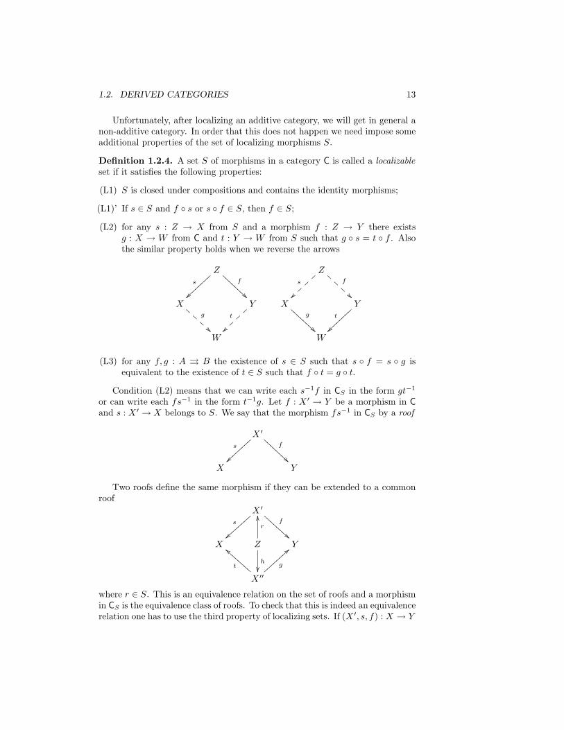
(L2) for any s : Z → X from S and a morphism f : Z → Y there existsg : X → W from C and t : Y → W from S such that g s = t f . Alsothe similar property holds when we reverse the arrows
Zs
~~
f
AAA
AAAA
A
Xg
BB
BB Y
t
~~
W
Zs
~~
f
AA
AA
Xg
BBB
BBBB
B Yt
~~
W
(L3) for any f, g : A ⇒ B the existence of s ∈ S such that s f = s g isequivalent to the existence of t ∈ S such that f t = g t.
Condition (L2) means that we can write each s−1f in CS in the form gt−1
or can write each fs−1 in the form t−1g. Let f : X ′ → Y be a morphism in Cand s : X ′ → X belongs to S. We say that the morphism fs−1 in CS by a roof
X ′
s
~~||||
|||| f
AAA
AAAA
A
X Y
Two roofs define the same morphism if they can be extended to a commonroof
X ′
s
||||
|||| f
!!BBB
BBBB
B
X Z
r
OO
h
Y
X ′′t
aaBBBBBBBB g
==||||||||
where r ∈ S. This is an equivalence relation on the set of roofs and a morphismin CS is the equivalence class of roofs. To check that this is indeed an equivalencerelation one has to use the third property of localizing sets. If (X ′, s, f) : X → Y
14 LECTURE 1. DERIVED CATEGORIES
is equivalent to (X ′′, t, g) by means of (Z ′, r, h) and (X ′′, t, g) is equivalent to(X ′′′, u, e) by means of (Z ′′, p, i), then we first define sr : Z ′ → X, tp : Z ′′ → X,then take v : W → Z ′, k : W → Z ′′ such that srv = tpk. Then f1 = hv, f2 = pksatisfy tf1 = tf2. Thus we find w : Z ′′′ → W such that f1w = f2w. If wetake q = rvw : Z ′′′ → X ′ and j = ikw : Z ′′′ → X ′′′ we get the equivalence(X ′, s, t) ∼ (X ′′′, u, e).
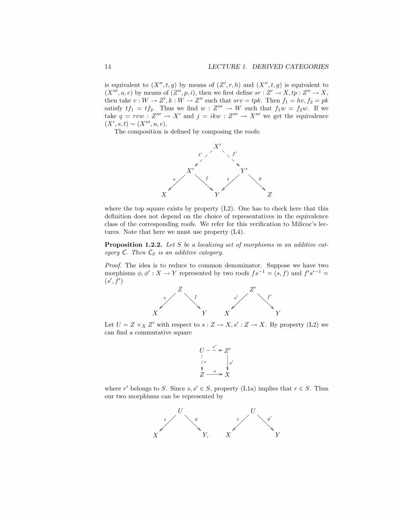
The composition is defined by composing the roofs:
X ′
t′
||
||
f ′
BB
BB
X ′
s
~~||||
|||| f
!!CCC
CCCC
C Y ′
t
||||
|||| g
AAA
AAAA
X Y Z
where the top square exists by property (L2). One has to check here that thisdefinition does not depend on the choice of representatives in the equivalenceclass of the corresponding roofs. We refer for this verification to Milicoc’s lec-tures. Note that here we must use property (L4).
Proposition 1.2.2. Let S be a localizing set of morphisms in an additive cat-egory C. Then CS is an additive category.
Proof. The idea is to reduce to common denominator. Suppose we have twomorphisms φ, φ′ : X → Y represented by two roofs fs−1 = (s, f) and f ′s′−1 =(s′, f ′)
Zs
~~~~~~
~~~
f
@@@
@@@@
X Y
Z ′
s′
~~
f ′
AAA
AAAA
X Y
Let U = Z ×X Z ′ with respect to s : Z → X, s′ : Z → X. By property (L2) wecan find a commutative square
Ur′ //___
r
Z ′
s′
Z
s // X
where r′ belongs to S. Since s, s′ ∈ S, property (L1a) implies that r ∈ S. Thusour two morphisms can be represented by
Ut
~~~~
~~~~ g
@@@
@@@@
X Y,
Ut
~~~~~~
~~~
g′
@@@
@@@@
X Y
1.2. DERIVED CATEGORIES 15
where t = sr = s′ r′, g = f r, g′ = f ′ r′. It remains to define the sum φ+φ′
as the morphism represented by the roof X t←− U g+g′−→ Y .Next observe that the zero morphism 0 : X → Y is equivalent to any roof of
the formXs←− X ′ 0−→ Y . They are related by the morphismX ′ 1←− X ′ f−→ X.
In particular, the zero object 0 in C is the zero object in CS since EndCS(0) =
0. Finally, the direct sum in CS is represented by the direct sum in C andthe canonical injections and the projections are defined by the correspondingmorphisms in C.
Note that one can prove the proposition without using property (F1a) (seeMilicic’s Lectures, www.math.utah.edu/ milicic/dercat.pdf). However it greatlysimplifies the proof and it is checked in the case of derived categories.
Since replacing a morphism of complexes by a homotopy equivalent mor-phism does not change the map on the cohomology, the definition of a quasi-isomorphism extends to the category K(A).
It turns out that the set of quasi-isomorphisms in K(A) is a localizing set(but not in Cp(A)). We will see later that the corresponding localization ofK(A) is equivalent to the derived category D(A).
Before we show that the set of quasi-isomorphisms in K(A) is a localizingset we have to introduce some constructions familiar from homotopy theory.
Recall the cone construction from algebraic topology. Let f : X → Y bea continuous map of topological spaces. We define the cone C(f) of f as thetopological space
C(f) = Y∐
X × [0, 1]/ ∼,
where (x, 1) ∼ f(x) and (x, 0) ∼ (x0, 0) for some fixed x0 ∈ X. In the caseY is a point, C(f) = ΣX is the suspension of X (ΣX is a ‘double cone’, it isobtained from X × [0, 1] with X × 0 and X × 1 identified with a point).In the case when X → Y is an inclusion, C(f) is homotopy equivalent to Y/X(the space obtained by contracting Y to a point). So in this case C(f) is ananalog of a cokernel. Also note that there is an inclusion Y → C(f) and if weapply the cone construction to this we get that C(f)/Y is homotopy equivalentto ΣX. Thus we have a sequence of morphisms in the homotopy category:
X → Y → C(f)→ ΣX.
Recall that we have the suspension isomorphism:
Hi+1(ΣX) ∼= Hi(X),
andHi(C(f)) = Hi(Y,X).
This gives a long exact sequence
. . .→ Hi(X)→ Hi(Y )→ Hi(Y,X)→ Hi−1(X)→ Hi−1(Y )→ . . .
16 LECTURE 1. DERIVED CATEGORIES
There is an analogous construction of the cone C(f) of a morphism f : X →Y of simplicial complexes which is I am not going to remind. The cochaincomplex of C(f) is
C•(C(f)) = C•(X)[1]⊕ C•(Y ), d =(dX [1] 0f [1] dY
)in the sense that (a, b) ∈ Ci+1(X)⊕Ci(Y ) goes to (di+1
X (a), f i+1(a) + diY (b)) ∈Ci+2(X) ⊕ Ci+1(Y ). This can be taken for the definition of the cone C(f) forany morphism of cochain complexes f : X• → Y • in Cp(A).
Definition 1.2.5. Let f : X• → Y • be a morphism in Cp(A). Define the coneof f as the complex
C(f) = X•[1]⊕ Y •, d =(dX•[1] 0f [1] dY •
).
Define the cylinder Cyl(f) as the complex
Cyl(f) = X• ⊕X•[1]⊕ Y •, d =
dX• −1 00 dX•[1] 00 f [1] dY •
.
Example 1.2.3. Let f : X → Y be a morphism in A considered as a morphismof complexes with support at 0. Then (C(f))−1 = X,C(f)0 = Y and d = f .Thus H0(C(f)) = ker(f) and H1(C(f)) = coker(f).
Example 1.2.4. Take f = idK• : K• → K•. Let ki : Xi+1 ⊕Xi → Xi ⊕Xi−1
defined by (xi+1, xi) → (xi, 0) This defines the homotopy between idC(f) and0C(f). In particular, all cohomology of the complex C(f) vanish.
Lemma 1.2.5. Let f : X• → Y • be a morphism of complexes. There is acommutative diagram in Cp(A):
0 // Y •if //
α
C(f)pf // X•[1] // 0
0 // X• //
f
Cyl(f) //
β
C(f) // 0
X• f // Y •
Its rows are exact and the vertical arrows are quasi-isomorphisms.
Proof. Let us describe the morphisms in this diagram. The morphism if : Y • →C(f) = X•[1]⊕Y • is the direct sum inclusion. The morphism pf : C(f)→ X•[1]is the projection to the first summand. The morphism Cyl(f) = X• ⊕X•[1]⊕Y • → X•[1]⊕ Y • is the projection to the last two summands. We take α to be
1.2. DERIVED CATEGORIES 17
the direct sum inclusion and β = (f,⊕idY •). The morphism f : X• → Cyl(f)is the direct sum inclusion. We leave to the reader to check that this definesmorphisms of complexes, the diagram is commutative and its rows are exact.
Obviously, βα = idY • Let us check that αβ is homotopy equivalent to theidentity. We define the homotopy hi : Cyl(f)ii → Cyl(f)i−1 by (xi, xi+1, li) =(0, xi, 0). We have
α β(xi, xi+1, li) = (0, 0, f(xi+1) + li),
(di−1Cyl(f)h
i+hidiCyl(f))(xi, xi+1, li) = (−xi,−diX•(xi), f(xi))+(0, diK(xi)−xi+1, 0) =
(−xi,−xi+1, f(xi+1)) = (α β − idCyl(f))(xi, xi+1, li).
This checks that α β ∼ idY • .
Corollary 1.2.6. Let f : X• → Y • be a morphism in K(A). Then it can beextended to a sequence
X• f // Y •g // C(f) h // X•[1] ,
where the composition of any two morphisms is zero.
Proof. We define g : Y • → C(f) = X•[1] ⊕ Y • and h : C(f) → X•[1] as inthe first row of the diagram from the lemma. By the proof of the previouslemma, the composition g f : X• → Y • → C(f) is homotopy equivalentto the composition X• → Cyl(f) → C(f) which is zero. The compositionhg : Y • → C(f)→ X•[1] is zero because the top row in the lemma is an exactsequence.
Definition 1.2.6. A triangle in Cp(A) is a diagram of the form
X• → Y • → Z• → X•[1].
A distinguished triangle is a triangle which is quasi-isomorphic to the triangle
X• f−→ Y •if−→ C(f)
pf−→ X•[1].
It follows from Lemma 1.2.5 that a distinguished triangle is quasi-isomorphicto the triangle
X• → Cyl(f)→ C(f)→ X•[1]
with morphisms defined in the lemma.
Lemma 1.2.7. Any short exact sequence of complexes is quasi-isomorphic tothe middle row of the diagram from Lemma 1.2.5.
Proof. Let
0→ X• f→ Y •g→ Z• → 0
18 LECTURE 1. DERIVED CATEGORIES
be an exact sequence in Cp(A). We define β : Cyl(f) → Y • to be equal toβ from Lemma 1.2.5 and γ : C(f) → Z• by composing the natural projectionC(f)→ Y • with g. We have ker(γ) = X•[1]⊕ im(f) = X•[1]⊕X• = C(idX•).By Example 1.2.4, the latter complex has trivial cohomology. Thus, using theexact sequence 0 → ker(γ) → C(f) → Z• → 0 we obtain that γ is a quasi-isomorphism.
Theorem 1.2.8. Any distinguished triangle
X• → Y • → Z• → X•[1]
defines an exact sequence of cohomology:
. . .→ Hi(X•)→ Hi(Y •)→ Hi(Z•)→ Hi(X•[1]) = Hi+1(X•)→ . . . . (1.2)
Proof. It is enough to prove it for the distinguished triangle:
X• → Cyl(f)→ C(f)g→ X•[1].
We have the exact sequence
0→ X• → Cyl(f)→ C(f)→ 0.
It gives the exact sequence of cohomology
. . .→ Hi(X•)→ Hi(Cyl(f))→ Hi(C(f)) δ→ Hi+1(X•)→ . . . .
It remains to identify the coboundary morphism δ with Hi(g). We use thatCyl(f)i = Xi ⊕ C(f)i and check the definitions.
Theorem 1.2.9. In the category K(A) quasi-isomorphims form a localizing setof morphisms.
Proof. Properties (L1) and (L1’) are obvious.Let t : Y • → W • and g : X• → W •, where t is a quasi-isomorphism. We
have to find a quasi-isomorphism s : Z• → X• and a morphism of complexesf : Z• → Y • such that f t = s g. Let X• → C(t) be the composition it g,where it : W → C(t) is the canonical inclusion. Let s : C(it g)[−1] → X• bethe morphism pitg[−1], where pitg : C(it g) = X•[1] ⊕ C(f) → X•[1] is thecanonical projection. We have the following diagram
C(it g)[−1]
f
s // X• itg //
g
C(t) // C(it g)
f [1]
Y •
t // W • it // C(t) // Y •[1]
where the morphism f is constructed as follows. An element from C(it g)[−1]is a triple (xi, yi, wi−1) ∈ Xi⊕Y i⊕W i−1. We set f(xi, yi, wi−1) = −yi. I claim
1.2. DERIVED CATEGORIES 19
that this diagram is commutative in the category K(A) (but not in Cp(A)!). Wehave
g s− t f(xi, yi, wi−1) = g(xi)− t(yi),
Let χ = χi, where χi : C(it g)[−1]i = C(it g)i−1 → W i−1 is given byχi(xi, yi, wi−1) = −wi−1. We have
(χ dC(itg)[−1] + dW• χ)((xi, yi, wi−1)
= χ((dX•(xi), dY •(yi),−dW•(wi−1)− t(xi)− g(xi)) + dW•(−wi−1) =
dW•(wi−1)− t(xi) + g(xi)− dW•(wi−1) = g(xi)− t(yi).
This shows that g s− t f is homotopy to zero. It remains to show that s isa quasi-isomorphism. Since t is a quasi-isomorphism, exact sequence of coho-mology (1.2) implies that all cohomology of C(f) are equal to zero. Applyingthe same exact sequence to the top row of the diagram, we obtain that s is aquasi-isomorphism.
To finish the verification of property (L2) we have also verify that a pairs : Z• → X•, f : Z• → Y •, where s is a quasi-isomorphism, defines a pairg : X• → W •, t : Y • → W •, where t is a quasi-isomorphism, and g s = t f .This follows from a similar argument using the following commutative diagramin K(A):
C(s)[−1] τ // Z•s //
f
X• //
g
C(s)
C(s)[−1]fτ // Y •
t // C(f τ) // C(s)
We leave it to the reader.Finally we have to check property (L3). Let f : X• → Y • be a morphism in
K(A). Assume s f = 0 in K(A) for some quasi-isomorphism s : Y • → Z•. Lethi : X• → Z•[−1] defines a homotopy between s f and the zero morphism.We have to find a quasi-isomorphism t : W • → X• and a homotopy betweenf t and the zero morphism. Consider the following commutative diagram:
C(s)[−1] // Y •s // Z•
C(s)[−1] X•goo_ _ _
f
OO
C(g)[−1]too_ _ _
where the morphism g : X• → C(s)[−1] is defined by gi(xi) = (f i(xi),−hi(xi))and t is the natural projection. Then t f = 0 because t g = 0. Also t is aquasi-isomorphism because s is a quasi-isomorphism and hence C(s) has trivialhomology. A similar assertion with the roles of s and t reversed can be provenin analogous manner.
20 LECTURE 1. DERIVED CATEGORIES
It remains to show that the localization of K(A) with respect to the localizingset of quasi-isomorphisms is equivalent to the derived category D(A). By theuniversality property we have a functor from D(A) → K(AS), where S is theset of quasi-isomorphisms. This functor is bijective on the sets of objects andsurjective on the set of morphisms. It remains to show that it is injective onthe set of morphisms. This follows from the following lemma.
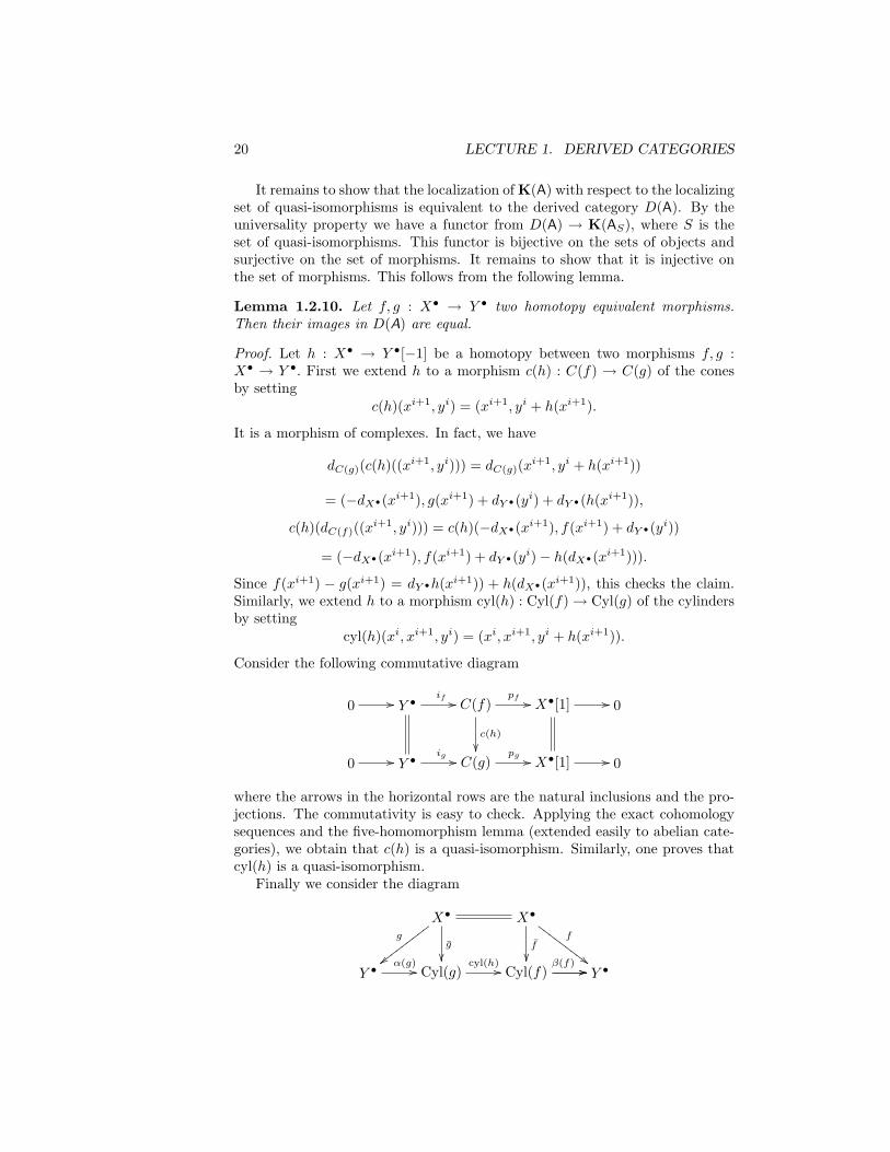
Lemma 1.2.10. Let f, g : X• → Y • two homotopy equivalent morphisms.Then their images in D(A) are equal.
Proof. Let h : X• → Y •[−1] be a homotopy between two morphisms f, g :X• → Y •. First we extend h to a morphism c(h) : C(f) → C(g) of the conesby setting
c(h)(xi+1, yi) = (xi+1, yi + h(xi+1).
It is a morphism of complexes. In fact, we have
dC(g)(c(h)((xi+1, yi))) = dC(g)(xi+1, yi + h(xi+1))
= (−dX•(xi+1), g(xi+1) + dY •(yi) + dY •(h(xi+1)),
c(h)(dC(f)((xi+1, yi))) = c(h)(−dX•(xi+1), f(xi+1) + dY •(yi))
= (−dX•(xi+1), f(xi+1) + dY •(yi)− h(dX•(xi+1))).
Since f(xi+1) − g(xi+1) = dY •h(xi+1)) + h(dX•(xi+1)), this checks the claim.Similarly, we extend h to a morphism cyl(h) : Cyl(f)→ Cyl(g) of the cylindersby setting
cyl(h)(xi, xi+1, yi) = (xi, xi+1, yi + h(xi+1)).
Consider the following commutative diagram
0 // Y •if // C(f)
pf //
c(h)
X•[1] // 0
0 // Y •ig // C(g)
pg // X•[1] // 0
where the arrows in the horizontal rows are the natural inclusions and the pro-jections. The commutativity is easy to check. Applying the exact cohomologysequences and the five-homomorphism lemma (extended easily to abelian cate-gories), we obtain that c(h) is a quasi-isomorphism. Similarly, one proves thatcyl(h) is a quasi-isomorphism.
Finally we consider the diagram
X•
g
g
wwww
wwww
wX•
f
f
##GGG
GGGG
GG
Y •α(g) // Cyl(g)
cyl(h) // Cyl(f) //β(f) // Y •
1.2. DERIVED CATEGORIES 21
Here we employ the notation α(f), β(f) and α(g), β(g)f , g from Lemma1.2.5. One easily checks that the square and the right triangle are commutative.The left triangle becomes commutative in D(A). In fact we know from Lemma1.2.5 that α(g) has the inverse β(g). Since g = β(g) g, we have α(g) g = gin D(A). This implies that left triangle is commutative in D(A). Finally onechecks that β(f) cyl(h) α(g) = idY • , hence the images of f and g in D(A)are equal.
A generalization of the notion of the derived category of an abelian categoryis the notion of a triangulated category.
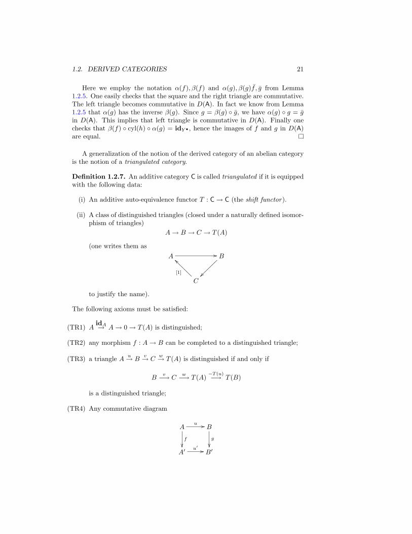
Definition 1.2.7. An additive category C is called triangulated if it is equippedwith the following data:
(i) An additive auto-equivalence functor T : C→ C (the shift functor).
(ii) A class of distinguished triangles (closed under a naturally defined isomor-phism of triangles)
A→ B → C → T (A)
(one writes them asA // B
~~~~
~~~
C
[1]
__@@@@@@@
to justify the name).
The following axioms must be satisfied:
(TR1) AidA→ A→ 0→ T (A) is distinguished;
(TR2) any morphism f : A→ B can be completed to a distinguished triangle;
(TR3) a triangle A u→ Bv→ C
w→ T (A) is distinguished if and only if
Bv−→ C
w−→ T (A)−T (u)−→ T (B)
is a distinguished triangle;
(TR4) Any commutative diagram
Au //
f
B
g
A′
u′ // B′
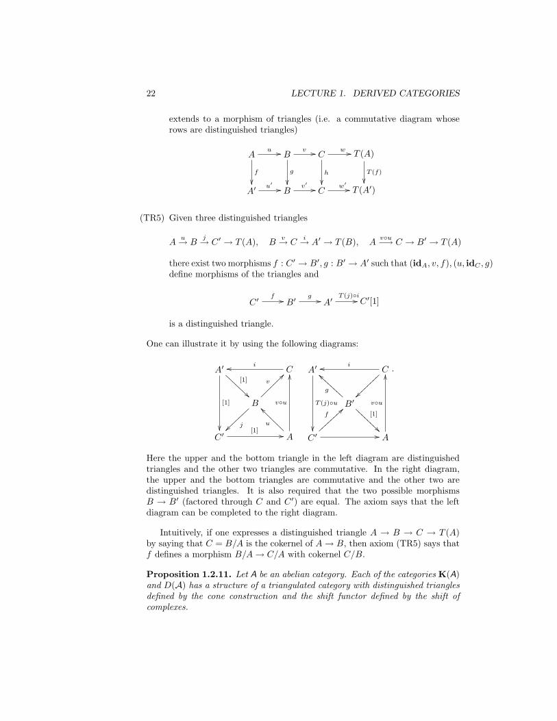
22 LECTURE 1. DERIVED CATEGORIES
extends to a morphism of triangles (i.e. a commutative diagram whoserows are distinguished triangles)
Au //
f
Bv //
g
Cw //
h
T (A)
T (f)
A′
u′ // Bv′ // C
w′ // T (A′)
(TR5) Given three distinguished triangles
Au→ B
j→ C ′ → T (A), Bv→ C
i→ A′ → T (B), Avu−→ C → B′ → T (A)
there exist two morphisms f : C ′ → B′, g : B′ → A′ such that (idA, v, f), (u, idC , g)define morphisms of the triangles and
C ′f // B′
g // A′T (j)i// C ′[1]
is a distinguished triangle.
One can illustrate it by using the following diagrams:
A′
[1]
AAA
AAAA
[1]
Cioo
B
v
??~~~~~~~
j~~
C ′[1] // A
u
__@@@@@@@
vu
OO A′
T (j)u
Cioo
~~~~~~
~~~~
B′
g
``BBBBBBBB
[1]
AAA
AAAA
A
C ′
f>>||||||||
// A
vu
OO .
Here the upper and the bottom triangle in the left diagram are distinguishedtriangles and the other two triangles are commutative. In the right diagram,the upper and the bottom triangles are commutative and the other two aredistinguished triangles. It is also required that the two possible morphismsB → B′ (factored through C and C ′) are equal. The axiom says that the leftdiagram can be completed to the right diagram.
Intuitively, if one expresses a distinguished triangle A → B → C → T (A)by saying that C = B/A is the cokernel of A→ B, then axiom (TR5) says thatf defines a morphism B/A→ C/A with cokernel C/B.
Proposition 1.2.11. Let A be an abelian category. Each of the categories K(A)and D(A) has a structure of a triangulated category with distinguished trianglesdefined by the cone construction and the shift functor defined by the shift ofcomplexes.
1.2. DERIVED CATEGORIES 23
Proof. Let us first check that K(A) is a triangulated category. Axiom (TR1)follows from Example 1.2.4 since the cone C(idA) of the identity morphism ishomotopy to zero morphism, hence C(idA) ∼= 0 in K(A).
Axiom (TR2) follows from Corollary 1.2.6.Axiom (TR3) follows from Lermma 1.2.5 where we replace the morphism f
with the morphism f [−1] : X•[−1]→ Y •[−1] and apply Corollary 1.2.6.Axiom (TR4) is immediate. We may assume that C = C(u), C ′ = C(u′)
and take h = f [1]⊕ g.We skip the verification of axiom (TR5) since we are not going to use this
property (see [Gelfand-Manin] or [Kashiwara]).To check that D(A) is a triangulated category, we use a more general asser-
tion. Suppose C is a triangulated category and S is a localizing set of morphismsin C satisfying the following additional properties
(L4) s ∈ S if and only if s[1] belongs to S;
(L5) if in axiom (TR4) the morphisms f, g belong to S, the morphism h belongsto S.
Then we claim that CS inherits the structure of a triangulated category. For any
morphism u in CS represented by a roof A A′soo f // B we can define the
shift T (u) as the morphism represented by the roof A[1] A′[1]s[1]oo f [1] // B[1] .
It is easy to check that it does not depend on the choice of a representative roof.This defines the shift functor in CS . We define distinguished triangles in CS astriangles A → B → C → A[1] isomorphic (in CS) to distinguished triangles inC.
Now, axiom (TR1) becomes obvious. Suppose u : A→ B is represented by
a roof (s, f) as above. Let A′f→ B
v→ C → A′[1] be a distinguished trianglein C. Then it is isomorphic to the triangle A u→ B
v→ C → A′[1] in CS . Thischecks axion (TR2). Axiom (TR3) follows immediately from Axiom (TR3) inC.
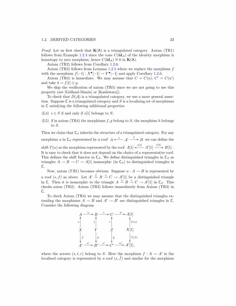
To check Axiom (TR4) we may assume that the distinguished triangles ex-tending the morphisms A → B and A′ → B′ are distinguished triangles in C.Consider the following diagram
Au // B
v // Cw // A[1]
X
s
OO
f
Y
t
OO
g
Z
r
OO
h
X[1]
T (s)
OO
T (f)
A′
u′ // B′v′ // C ′
w′ // A′[1],
where the arrows (s, t, r) belong to S. Here the morphism f : A → A′ in thelocalized category is represented by a roof (s, f) and similar for the morphism
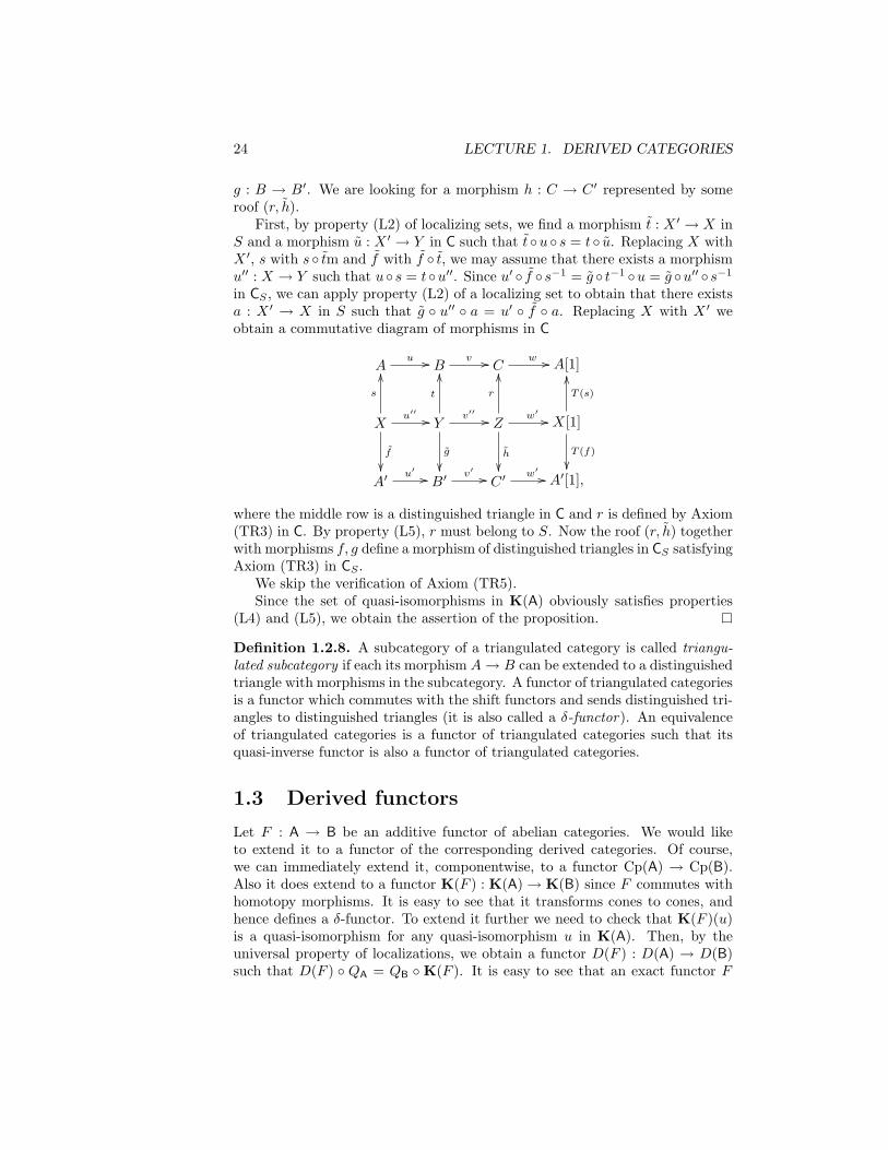
24 LECTURE 1. DERIVED CATEGORIES
g : B → B′. We are looking for a morphism h : C → C ′ represented by someroof (r, h).
First, by property (L2) of localizing sets, we find a morphism t : X ′ → X inS and a morphism u : X ′ → Y in C such that t u s = t u. Replacing X withX ′, s with s tm and f with f t, we may assume that there exists a morphismu′′ : X → Y such that u s = tu′′. Since u′ f s−1 = g t−1 u = g u′′ s−1
in CS , we can apply property (L2) of a localizing set to obtain that there existsa : X ′ → X in S such that g u′′ a = u′ f a. Replacing X with X ′ weobtain a commutative diagram of morphisms in C
Au // B
v // Cw // A[1]
X
s
OO
f
u′′ // Y
t
OO
g
v′′ // Z
r
OO
h
w′ // X[1]
T (s)
OO
T (f)
A′
u′ // B′v′ // C ′
w′ // A′[1],
where the middle row is a distinguished triangle in C and r is defined by Axiom(TR3) in C. By property (L5), r must belong to S. Now the roof (r, h) togetherwith morphisms f, g define a morphism of distinguished triangles in CS satisfyingAxiom (TR3) in CS .
We skip the verification of Axiom (TR5).Since the set of quasi-isomorphisms in K(A) obviously satisfies properties
(L4) and (L5), we obtain the assertion of the proposition.
Definition 1.2.8. A subcategory of a triangulated category is called triangu-lated subcategory if each its morphism A→ B can be extended to a distinguishedtriangle with morphisms in the subcategory. A functor of triangulated categoriesis a functor which commutes with the shift functors and sends distinguished tri-angles to distinguished triangles (it is also called a δ-functor). An equivalenceof triangulated categories is a functor of triangulated categories such that itsquasi-inverse functor is also a functor of triangulated categories.
1.3 Derived functors
Let F : A → B be an additive functor of abelian categories. We would liketo extend it to a functor of the corresponding derived categories. Of course,we can immediately extend it, componentwise, to a functor Cp(A) → Cp(B).Also it does extend to a functor K(F ) : K(A)→ K(B) since F commutes withhomotopy morphisms. It is easy to see that it transforms cones to cones, andhence defines a δ-functor. To extend it further we need to check that K(F )(u)is a quasi-isomorphism for any quasi-isomorphism u in K(A). Then, by theuniversal property of localizations, we obtain a functor D(F ) : D(A) → D(B)such that D(F ) QA = QB K(F ). It is easy to see that an exact functor F
1.3. DERIVED FUNCTORS 25
transforms quasi-isomorphism to quasi-isomorphisms, but this is a very specialcase.
Let F : K(A)→ K(A) be a functor of triangulated categories in the sense ofDefinition 1.2.8. Note that we do not assume that F is of the form K(F ). Ob-viously, F extends to derived categories if it transforms quasi-isomorphisms toquasi-isomorphisms, and, in particularly, acyclic complexes (i.e. with zero coho-mology) to acyclic complexes. In this case it becomes a functor of triangulatedcategories. Also by considering
Conversely, suppose F is a functor of triangulated categories. Let f : X• →Y • be a quasi-isomorphism of complexes from K(A). Extending it to a dis-tinguished triangle X• → Y • → C(f) → X•[1] we obtain an acyclic complexC(f) (apply the exact cohomology sequence). Consider the distinguished tri-angle F(X)• → F(Y )• → F(C(f)) → F(X)•[1]. If moreover we know that Ftransforms acyclic complexes to acyclic complexes, then F(C(f)) is acyclic, andF(X)• → F(Y )• is a quasi-isomorphism. The idea of defining the derived func-tor is to find a sufficiently large subcategory of K(A) such that the restrictionof F to it transforms acyclic complexes to acyclic complexes.
In the following Cp∗(A) denotes either Cp(A), or Cp±(A), or Cpb(A) andsimilar definitions for K∗(A), D∗(A).
Definition 1.3.1. A full triangulated subcategory K∗(A)′ of K∗(A) is calledleft (right) adapted for a left (right) exact functor F if the following propertiesare satisfied
(A1) F(X•) is acyclic for any acyclic complex X• in K∗(A)′;
(A2) for any object in X• in K∗(A) there is a quasi-isomorphism X• → R•
(R• → X•), where R• is an object in K∗(A)′;
(A3) the inclusion of categories ι : K∗(A)′ → K∗(A) defines an equivalence oftriangulated categories Ψ : K∗(A)′qis → D∗(A), where qis is the set ofquasi-isomorphisms.
By property (A1), F ι transforms acyclic complexes to acyclic complexes.By the universality property of localizations this defines a functor F : K∗(A)′qis →D∗(A) such thatQBFι = FQ′A. Let Φ : D∗(A)→ K∗(A)′qis be a quasi-inversefunctor. We set
D∗(F)′ = F Φ.
By property (A3), the functor D∗(F)′ is a functor of triangulated categories.
26 LECTURE 1. DERIVED CATEGORIES
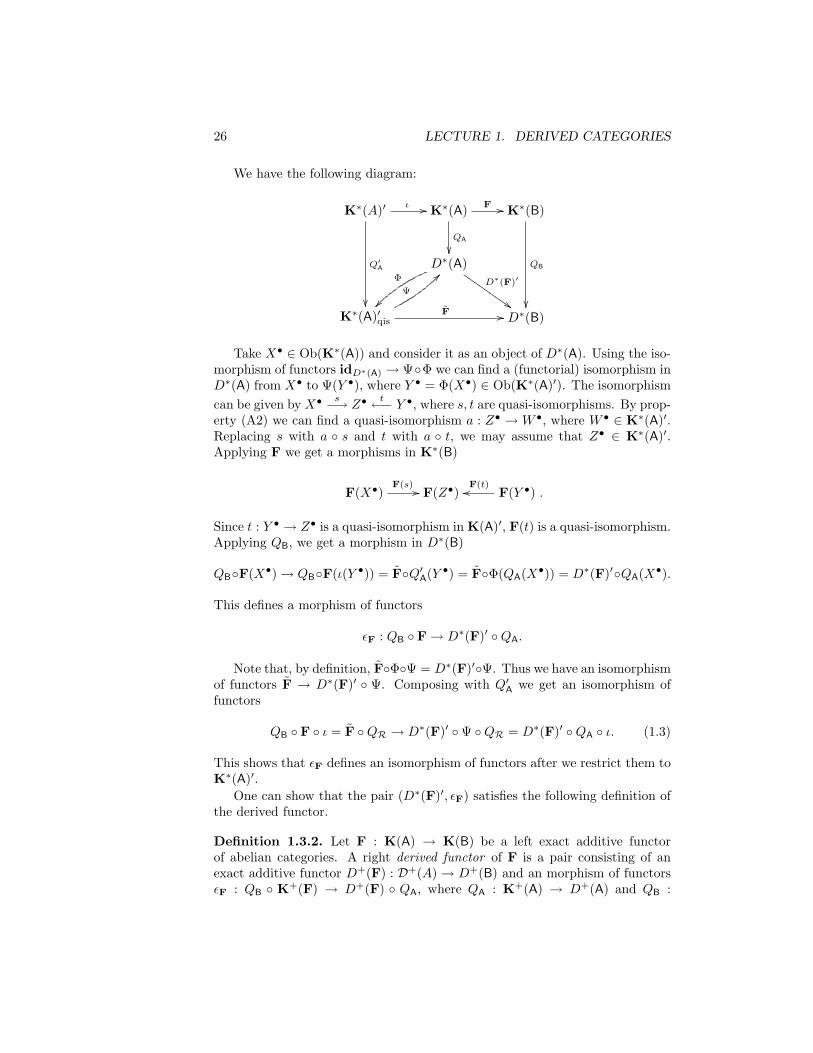
We have the following diagram:
K∗(A)′ ι //
Q′A
K∗(A) F //
QA
K∗(B)
QB
D∗(A)D∗(F)′
$$IIIIIIIII
Φ
K∗(A)′qis
Ψ
??
F // D∗(B)
Take X• ∈ Ob(K∗(A)) and consider it as an object of D∗(A). Using the iso-morphism of functors idD∗(A) → ΨΦ we can find a (functorial) isomorphism inD∗(A) from X• to Ψ(Y •), where Y • = Φ(X•) ∈ Ob(K∗(A)′). The isomorphismcan be given by X• s−→ Z•
t←− Y •, where s, t are quasi-isomorphisms. By prop-erty (A2) we can find a quasi-isomorphism a : Z• → W •, where W • ∈ K∗(A)′.Replacing s with a s and t with a t, we may assume that Z• ∈ K∗(A)′.Applying F we get a morphisms in K∗(B)
F(X•)F(s) // F(Z•) F(Y •)
F(t)oo .
Since t : Y • → Z• is a quasi-isomorphism in K(A)′, F(t) is a quasi-isomorphism.Applying QB, we get a morphism in D∗(B)
QBF(X•)→ QBF(ι(Y •)) = FQ′A(Y •) = FΦ(QA(X•)) = D∗(F)′QA(X•).
This defines a morphism of functors
εF : QB F→ D∗(F)′ QA.
Note that, by definition, FΦΨ = D∗(F)′Ψ. Thus we have an isomorphismof functors F → D∗(F)′ Ψ. Composing with Q′A we get an isomorphism offunctors
QB F ι = F QR → D∗(F)′ Ψ QR = D∗(F)′ QA ι. (1.3)
This shows that εF defines an isomorphism of functors after we restrict them toK∗(A)′.
One can show that the pair (D∗(F)′, εF) satisfies the following definition ofthe derived functor.
Definition 1.3.2. Let F : K(A) → K(B) be a left exact additive functorof abelian categories. A right derived functor of F is a pair consisting of anexact additive functor D+(F) : D+(A)→ D+(B) and an morphism of functorsεF : QB K+(F) → D+(F) QA, where QA : K+(A) → D+(A) and QB :
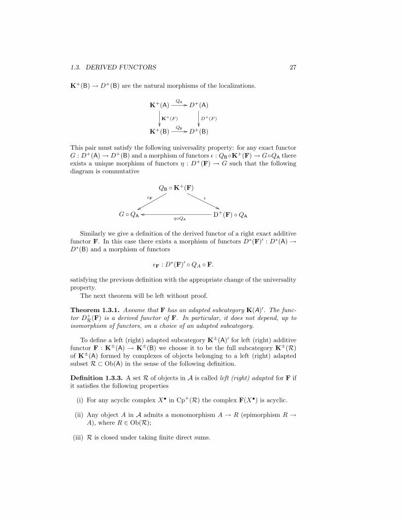
1.3. DERIVED FUNCTORS 27
K+(B)→ D+(B) are the natural morphisms of the localizations.
K+(A)QA //
K+(F )
D+(A)
D+(F )
K+(B)
QB // D+(B)
This pair must satisfy the following universality property: for any exact functorG : D+(A)→ D+(B) and a morphism of functors ε : QBK+(F)→ GQA thereexists a unique morphism of functors η : D+(F) → G such that the followingdiagram is commutative
QB K+(F)εF
xxqqqqqqqqqqqε
''OOOOOOOOOOO
G QA D+(F) QAηQA
oo
Similarly we give a definition of the derived functor of a right exact additivefunctor F. In this case there exists a morphism of functors D∗(F)′ : D∗(A) →D∗(B) and a morphism of functors
εF : D∗(F)′ QA F.
satisfying the previous definition with the appropriate change of the universalityproperty.
The next theorem will be left without proof.
Theorem 1.3.1. Assume that F has an adapted subcategory K(A)′. The func-tor D+
R(F) is a derived functor of F. In particular, it does not depend, up toisomorphism of functors, on a choice of an adapted subcategory.
To define a left (right) adapted subcategory K±(A)′ for left (right) additivefunctor F : K±(A) → K±(B) we choose it to be the full subcategory K±(R)of K±(A) formed by complexes of objects belonging to a left (right) adaptedsubset R ⊂ Ob(A) in the sense of the following definition.
Definition 1.3.3. A set R of objects in A is called left (right) adapted for F ifit satisfies the following properties
(i) For any acyclic complex X• in Cp+(R) the complex F(X•) is acyclic.
(ii) Any object A in A admits a monomorphism A → R (epimorphism R →A), where R ∈ Ob(R);
(iii) R is closed under taking finite direct sums.
28 LECTURE 1. DERIVED CATEGORIES
We will show that K±(R) is an adapted subcategory for F : K+(A) →K+(B). This will allow us to define the derived functor
D+R(F) : D+(A)→ D+(B).
By above we obtain a morphism of functors
εF : QB K+(F)→ D+R(F) QA.
Lemma 1.3.2. Any X• ∈ K+(A) admits a quasi-isomorphism to an object inK+(R).
Proof. Without loss of generality we may assume that Xp = 0, p < 0. Leti0 : X0 → R0 be a monomorphism of X0 to an object from R. Let R0 qX0 X1
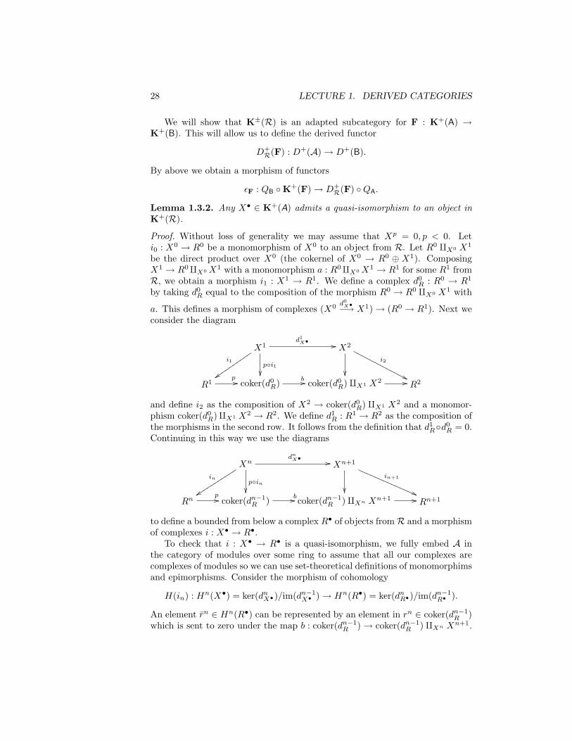
be the direct product over X0 (the cokernel of X0 → R0 ⊕ X1). ComposingX1 → R0qX0X1 with a monomorphism a : R0qX0X1 → R1 for some R1 fromR, we obtain a morphism i1 : X1 → R1. We define a complex d0
R : R0 → R1
by taking d0R equal to the composition of the morphism R0 → R0 qX0 X1 with
a. This defines a morphism of complexes (X0 d0X•−→ X1)→ (R0 → R1). Next weconsider the diagram
X1
i1
zzuuuuuuuuuupi1
d1X• // X2
i2
''NNNNNNNNNNNNN
R1p // coker(d0
R) b // coker(d0R)qX1 X2 // R2
and define i2 as the composition of X2 → coker(d0R) qX1 X2 and a monomor-
phism coker(d0R)qX1 X2 → R2. We define d1
R : R1 → R2 as the composition ofthe morphisms in the second row. It follows from the definition that d1
Rd0R = 0.
Continuing in this way we use the diagrams
Xn
in
yytttttttttttpin
dnX• // Xn+1
in+1
((QQQQQQQQQQQQQQ
Rnp // coker(dn−1
R ) b// coker(dn−1R )qXn Xn+1 // Rn+1
to define a bounded from below a complex R• of objects fromR and a morphismof complexes i : X• → R•.
To check that i : X• → R• is a quasi-isomorphism, we fully embed A inthe category of modules over some ring to assume that all our complexes arecomplexes of modules so we can use set-theoretical definitions of monomorphimsand epimorphisms. Consider the morphism of cohomology
H(in) : Hn(X•) = ker(dnX•)/im(dn−1X• )→ Hn(R•) = ker(dnR•)/im(dn−1
R• ).
An element rn ∈ Hn(R•) can be represented by an element in rn ∈ coker(dn−1R )
which is sent to zero under the map b : coker(dn−1R )→ coker(dn−1
R ) qXn Xn+1.
1.3. DERIVED FUNCTORS 29
Since coker(dn−1R ) qXn Xn+1 = coker(Xn → coker(dn−1
R ) ⊕ Xn+1), we obtainthat (rn, 0) must be the image of some element from Xn, in particular rn =p(in(xn)) for some xn ∈ Xn. Obviously, xn ∈ ker(dnX•). This checks that H(in)is surjective. We leave to the reader to check that H(in) is injective.
Proposition 1.3.3. Let R be an adapted set of objects for a left exact functorF. Then the subcategory K+(R) of K+(A) is an adapted subcategory.
Proof. Since the cone of a morphism of complexes in K+(R) is an object fromK+(R), the subcategory K+(R) is a triangulated subcategory of K+(A).
Property (A1) follows from the definition. Property (A2) follows from Lemma1.3.2.
It remains to verify (A3). Let us first show that the functor K+(R)qis →D+(A) is an equivalence of categories. Applying Lemma 1.3.2, it suffices toprove that this functor is fully faithful. Any morphism u : X• → Y • in D+(A)of objects from K+(R) is represented by a roof g : X• → Z•, t : Y • → Z•,where Z• is an object of K(A) and t is a quasi-isomorphism. Applying Lemma1.3.2, we find a quasi-isomorphism s : Z• →W •, where W ∈ K+(R). The roof(s t, s g) is a morphism u′ : X• → Y • in K+
qis such that Ψ(u′) = u. We leaveto the reader to check the injectivity of the map on Hom’s defined by Ψ. Thisproves the assertion.
Obviously, the set of quasi-isomorhisms in K+(A) is a localizing set satisfy-ing the additional properties (L4) and (L5). Thus K+(R)qis is a triangulatedcategory and the inclusion functor K+(R)→ K+(A) defines a functor of trian-gulated categories. To show that it is an equivalence of triangulated categories,we have to verify that its quasi-inverse functor is a functor of triangulated cat-egories. This follows from the lemma below.
Lemma 1.3.4. A triangle in K+(R)qis isomorphic to a distinguished trianglein D+(A) is isomorphic to a distinguished triangle with objects in R.
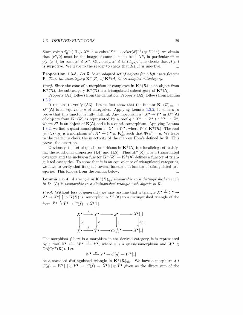
Proof. Without loss of generality we may assume that a triangle X• f→ Y • →Z• → X•[1] in K(R) is isomorphic in D+(A) to a distinguished triangle of the
form X• f→ Y • → C(f)→ X•[1].
X•
φ
f // Y • //
ψ
Z• //
γ
X•[1]
φ[1]
X•
f // Y • // C(f)• // X•[1]
The morphism f here is a morphism in the derived category, it is representedby a roof X• s←− W • g−→ Y •, where s is a quasi-isomorphism and W • ∈Ob(Cp+(R)). Let
W • g−→ Y • → C(g)→W •[1]
be a standard distinguished triangle in K+(R)qis. We have a morphism δ :C(g) = W •[1] ⊕ Y • → C(f) = X•[1] ⊕ Y • given as the direct sum of the
30 LECTURE 1. DERIVED CATEGORIES
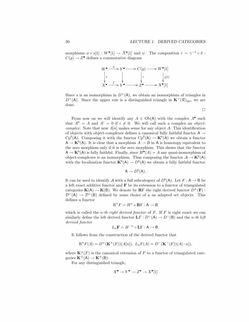
morphisms φ s[1] : W •[1] → X•[1] and ψ. The composition r = γ−1 δ :C(g)→ Z• defines a commutative diagram
W •
s
g // Y • //
C(g) //
r
W •[1]
g[1]
X• f // Y • // Z• // X•[1]
Since s is an isomorphism in D+(A), we obtain an isomorphism of triangles inD+(A). Since the upper row is a distinguished triangle in K+(R)qis, we aredone.
From now on we will identify any A ∈ Ob(A) with the complex A• suchthat A0 = A and Ai = 0 if i 6= 0. We will call such a complex an object-complex . Note that now A[n] makes sense for any object A. This identificationof objects with object-complexes defines a canonical fully faithful functor A →Cpb(A). Composing it with the functor Cpb(A) → Kb(A) we obtain a functorA→ Kb(A). It is clear that a morphism A→ B in A is homotopy equivalent tothe zero morphism only if it is the zero morphism. This shows that the functorA→ Kb(A) is fully faithful. Finally, since H•(A) = A any quasi-isomorphism ofobject-complexes is an isomorphism. Thus composing the functor A → Kb(A)with the localization functor Kb(A)→ Db(A) we obtain a fully faithful functor
A→ Db(A).
It can be used to identify A with a full subcategory of Db(A). Let F : A→ B bea left exact additive functor and F be its extension to a functor of triangulatedcategories K(A)→ K(B). We denote by RF the right derived functor D+(F) :D+(A) → D+(B) defined by some choice of a an adapted set objects. Thisdefines a functor
RnF = Hn RF : A→ B
which is called the n-th right derived functor of F . If F is right exact we cansimilarly define the left derived functor LF : D−(A)→ D−(B) and the n-th leftderived functor
LnF = H−n LF : A→ B.
It follows from the construction of the derived functor that
RnF (A) = D+(K+(F ))(A[n]), LnF (A) = D−(K−(F ))(A[−n]),
where K±(F ) is the canonical extension of F to a functor of triangulated cate-gories K±(A)→ K±(B).
For any distinguished triangle,
X• → Y • → Z• → X•[1]
1.3. DERIVED FUNCTORS 31
we have the distinguished triangle
RF(X•)→ RF(X•)→ RF(X•)→ RF(X•)[1]
that defines a long exact sequence of cohomology
· · · → Hn(RF(X•))→ Hn(RF(Y •))→ Hn(RF(Z•))→ Hn+1(RF(X•))→ · · · .
In particular, a short exact sequence of objects in A
0→ Af→ B → C → 0
considered as the distinguished triangle (see Lemma 1.2.7)
A→ Cyl(f)→ C(f)→ A[1]
defines a long exact sequence
0→ F (A)→ F (B)→ F (C)→ R1F (A)→ R1F (B)→ R1F (C)→ · · · .
Similarly, a right exact functor defines a long exact sequence
· · · → L1F (A)→ L1F (B)→ L1F (C)→ F (A)→ F (B)→ F (C)→ 0.
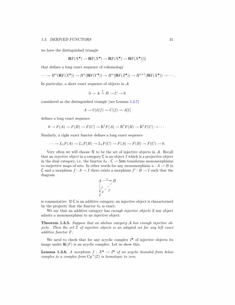
Very often we will choose R to be the set of injective objects in A. Recallthat an injective object in a category C is an object I which is a projective objectin the dual category, i.e. the functor hI : C→ Sets transforms monomorphismsto surjective maps of sets. In other words for any monomorphism u : A→ B inC and a morphism f : A→ I there exists a morphism f ′ : B → I such that thediagram
Au //
f
B
f ′~~
~~
I
is commutative. If C is an additive category, an injective object is characterizedby the property that the functor hI is exact.
We say that an additive category has enough injective objects if any objectadmits a monomorphism to an injective object.
Theorem 1.3.5. Suppose that an abelian category A has enough injective ob-jects. Then the set I of injective objects is an adapted set for any left exactadditive functor F .
We need to check that for any acyclic complex I• of injective objects itsimage under K(F ) is an acyclic complex. Let us show this.
Lemma 1.3.6. A morphism f : X• → I• of an acyclic bounded from belowcomplex to a complex from Cp+(I) is homotopic to zero.
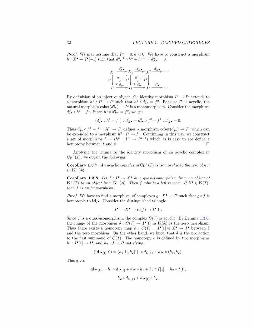
32 LECTURE 1. DERIVED CATEGORIES
Proof. We may assume that In = 0, n < 0. We have to construct a morphismh : X• → I•[−1] such that dn−1
I• hn + hn+1 dnX• = 0.
X0
f0
d0X• // X1
d1X• //
f1
h1
X2
f2
d2X• //
h2
· · ·
I0d0I• // I1
d1I• // I2d2I• // · · ·
By definition of an injective object, the identity morphism I0 → I0 extends toa morphism h1 : I1 → I0 such that h1 d0
I• = f0. Because I• is acyclic, thenatural morphism coker(d0
I•)→ I2 is a monomorphism. Consider the morphismd0I• h1 − f1. Since h1 d0
X• = f0, we get
(d0I• h1 − f1) d0
X• = d0I• f0 − f1 d0
X• = 0.
Thus d0I• h1 − f1 : X1 → I1 defines a morphism coker(d0
I•) → I1 which canbe extended to a morphism h2 : I2 → I1. Continuing in this way, we constructa set of morphisms h = (hn : In → In−1) which as is easy to see define ahomotopy between f and 0.
Applying the lemma to the identity morphism of an acyclic complex inCp+(I), we obtain the following.
Corollary 1.3.7. An acyclic complex in Cp+(I) is isomorphic to the zero objectin K+(A).
Corollary 1.3.8. Let f : I• → X• be a quasi-isomorphism from an object ofK+(I) to an object from K+(A). Then f admits a left inverse. If X• ∈ K(I),then f is an isomorphism.
Proof. We have to find a morphism of complexes g : X• → I• such that g f ishomotopic to idI• . Consider the distinguished triangle
I• → X• → C(f)→ I•[1].
Since f is a quasi-isomorphism, the complex C(f) is acyclic. By Lemma 1.3.6,the image of the morphism δ : C(f) → I•[1] in K(A) is the zero morphism.Thus there exists a homotopy map h : C(f) = I•[1] ⊕ X• → I• between δand the zero morphism. On the other hand, we know that δ is the projectionto the first summand of C(f). The homotopy h is defined by two morphismsh1 : I•[1]→ I•, and h2 : J → I• satisfying
(idI•[1], 0) = (h1[1], h2[1]) dC(f) + dI• (h1, h2).
This gives
idI•[1],= h1 dI•[1] + dI• h1 + h2 f [1] = h2 f [1],
h2 dC(f) + dI•[1] h2.
1.3. DERIVED FUNCTORS 33
This implies that h2 is a morphism of complexes and becomes the left inverseof f in K(A).
Suppose thatX• ∈ K(I). Since f has the left inverse, it must be a monomor-phism and h2 : X• → I• must be an epimorphism. Now we replace f with h2.Since f is a quasi-morphism, we get that h2 is a quasi-isomorphism. The previ-ous argument shows that h2 admits a left inverse, hence h2 is a monomorphismand, since it was an epimorphism, it must be an isomorphism. Therefore f isan isomorphism.
Remark 1.3.9. The same argument shows that all epimorphisms in K(A), andin particular in A, split if the category K(A) is abelian. In fact, assume f :X• → Y • is an epimorphism. Since K(A) is abelian, and the exact sequence0 → X → Cyl(f) → C(f) → 0 is isomorphic to the sequence X → Y →C(f) → 0 (see Lemma 1.2.5), we obtain that C(f) = 0 in K(A). This impliesthat C(f) → X•[1] is the zero morphism in K(A). Now we us the homotopyand the previous argument to construct the left inverse of u.
The previous corollary shows that the localization morphism K(I)→ K+(I)qis
is an equivalence of categories. Thus we obtain
Theorem 1.3.10. Assume that A has enough injective objects. Then
K+(I) ≈ D+(A).
An object-complex A is a special case of a complex X• ∈ Cp(A)+ suchthat Hi(X•) = 0, i 6= 0. A complex of this sort with Xi = 0 for i < 0 andH0(X•) ∼= X0 is called a resolution of X0. If R is a set of objects and allXi, i 6= 0, belong to R we call it an R-resolution. For example, we can defineinjective resolutions.
Let X• be a resolution of A. A choice of an isomorphism A → H0(X•)defines an acyclic complex
0→ A→ X0 → X1 → · · · → Xn → · · · .
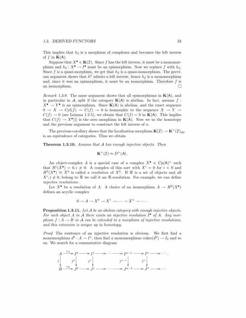
Proposition 1.3.11. Let A be an abelian category with enough injective objects.For each object A in A there exists an injective resolution I• of A. Any mor-phism f : A → B in A can be extended to a morphism of injective resolutions,and this extension is unique up to homotopy.
Proof. The existence of an injective resolution is obvious. We first find amonomorphism d0 : A→ I1, then find a monomorphism coker(d0)→ I2 and soon. We search for a commutative diagram
AeA //
f
I0 //
f0
I1 //
f1
· · · // In−1 //
fn−1
In //
fn
· · ·
BeB // J0 // J1 // · · · // Jn−1 // Jn // · · ·
.
34 LECTURE 1. DERIVED CATEGORIES
Since eA : A → I0 is a monomorphism, and J0 is injective, the compositioneB f : A→ J0 extends to a morphism f0 : I0 → J0 such that f0 eA = eB f .Assume that we can define fn in this way. Since dnJ fn d
n−1I = dnJ d
n−1J
fn−1 = 0 we see that fn defines a morphism from im(dnI ) to Jn+1. Since In+1
is injective we can extend it to a morphism fn+1 : In+1 → Jn+1. This extendsf to a morphism fn+1. This proves the existence of an extension.
Let us prove the second assertion. Let f , g be two extensions of f : A → Bto morphisms of the resolutions I• → J•. Obviously, f − g induce the zeromorphism on the cohomology. Then f − g is an extension of the zero morphismA → B. So, we may assume that f : A → B is the zero morphism. We needto show that the extension f is homotopy to zero. Since A → B → J0 iszero, we have a morphism coker(d0
I) → J0. Since J0 is injective, it extendsto a morphism h2 : I1 → J0. Clearly, f0 = h2 d1
I + h1 d0J , where h1 = 0.
Assume we can construct homotopy morphisms (hi), i ≤ n : In → Jn−1. Thusfn = hn+1 dnI +dn−1
J hn. Let α = fn+1−hn+1 dnI : In+1 → Jn+1. It is easyto see that dnJ α = 0. Thus α factors through im(dn+1
I ) and then extends tohn+1 : In+1 → Jn. We have fn+1 = kn+1 dn+1
I + dnJ tn+1 and, by induction,we are done.
Corollary 1.3.12. Suppose A has enough injective objects. Then A is equivalentto the full subcategory of K+(I) that consists of injective resolutions.
Proposition 1.3.13. Let F : A→ B be a left exact additive functor of abeliancategories. Suppose A has enough injective objects. There is an isomorphism offunctors
F ∼= R0F.
Proof. We take the set of injective objects as an adapted set of F and define thederived functor accordingly. Let I• be an injective resolution of A. It followsfrom the definitions that R0F (A) = H0(F (I•)). Since F is left exact, F (I0) =F (A) → F (I1) is a monomorphism. This shows that H0(F (I•)) ∼= F (A). Tomake this isomorphism functorial, we use that any morphism A → A′ in Adefines a unique morphism in K(A) of their injective resolutions. Since takingcohomology H0 is a functor K(A)→ B we see that R0F is isomorphic to F .
Note that, if the derived functor is defined by using an adapted set of ob-jects, we always have an isomorphism R0F (A) ∼= F (A) but we do not have anisomorphism of functors.
Example 1.3.14. We assume that A has enough injective objects. Considerthe additive functor F = HomA(A, ?) : B → HomA(A,B) from A to Ab. Bydefinition of a monomorphism, F is a left exact functor. We denote by
RHom(A, ?) : D+(A)→ D+(Ab)
its right derived functor. The functors Exti(A, ?) : A→ Ab are defined by
ExtiA(A, ?) := RiHomA(A, ?).
1.3. DERIVED FUNCTORS 35
Let us recall the definition. First we extend the functor HomA(A, ?) to a functorKHomA(A, ?) : K+(A)→ K+(Ab). By definition,
KHomA(A,X•) = Hom•(A,X•),
where Homi(A,X•) = HomA(A,Xi) = HomK(A)(A,X•[i]). To extend it to aderived functor, we replace X• with a quasi-isomorphic complex of injectiveobjects I• and apply the extended functor to I• to get
HomiA(A,X•) := Hi(RHom(A, I•)) ∼= HomK(A)(A, I•[n]))
∼= HomD+(A)(A,X•[n])).
If X• = B is an object-complex, then I• is an injective resolution of B, andHomi
A(A,B) coincides with the familiar definition of ExtiA(A,B) from homolog-ical algebra.
More generally, let A• and B• be two complexes in A, we define the complexof abelian groups Hom•(A•, B•) = (Hom•(A•, B•)n, dn) in A by setting
Hom•(A•, B•)n =∏i∈Z
HomA(Ai, Bi+n),
dn(fi) = dB• fi − (−1)nfi dA• , fi : Ai → Bi+n.
Note that the kernel of dn consists of morphisms A• → B•[n] in Cp(A) and theimage of dn−1 consists of morphisms of complexes homotopic to zero. Thus
Hn(Hom•(A•, B•)) ∼= HomK(A)(A•, B•[n]) ∼= HomK(A)(A•[−n], B•).
Via the composition of morphisms in Cp(A) we get a bi-functor
Hom•(?, ?) : Cp(A)op × Cp(A)→ Cp(A)
that can be extended to a bifunctor
Hom•(?, ?) : K(A)op ×K(A)→ K(Ab).
It follows easily from the definition that both partial functors are δ-functors.If A has a set of right adapted objects for the first partial functor (e.g. A hasenough projective objects), then we can extend Hom•(?, ?) to a bi-functor
RHom•(?, ?) : D−(A)op ×D+(A)→ Db(Ab).
The composition of both partial functors with the cohomology functor Hi :Db(Ab)→ Ab are isomorphic functors (so we may choose one, if only one partialfunctor is defined) and we set
HomiA(A•, B•) := Hi(Hom•(A•, B•)).
If the second partial derived functor exists, we have
HomiA(A•, B•) = HomD+(A)(A•, B•[i]).
36 LECTURE 1. DERIVED CATEGORIES
If the second partial derived functor exists, we have
HomiA(A•, B•) = HomD−(A)(A•[−i], B).
The restriction of the bifunctors HomiA(?, ?) to Aop×A and taking the cohomol-
ogy, we get the familiar bifunctors ExtiA(?, ?).
Example 1.3.15. Let (X,OX) be a ringed space. For any sheaf of right OX -modulesM and a sheaf of left OX -modules N one can define its tensor productM⊗OX
N . This is a just an abelian sheaf on X. If furthermore, M (resp.N ) has a structure of a OX -bimodule, then the tensor product is a sheaf ofleft (resp. right) OX -modules. In particular, this is true if OX is a sheaf ofcommutative rings. FixM and consider the functor
M⊗OX: Mod(OX)→ Shab
X , N →M⊗OXN .
This functor is right exact and, after passing to the homotopy category of com-plexes defines a δ-functor. Similarly, we define the right exact functor
⊗OXN : Mod(Oop
X )→ ShabX , M→M⊗OX
N .
A sheaf of OX -modules is called flat if the functorM⊗OXis exact. An example
of a flat sheaf is a locally free sheaf (maybe of infinite rank). Any sheaf of OX -modules admits a flat resolution. One uses the sheaves OU defined by
(OU )x =
OX,x if x ∈ U ,
0 otherwise,
where U is an open subset. Since we have a natural bijection HomOX(OU ,F)→
F(U), it is easy to see that the sheaf ⊕UOU is a projective generators inMod(OX).
The set of flat sheaves is a right adapted set for the functorM⊗OXand one
defines its left derived functor
ML⊗OX
: D−(Mod(OX))→ D−(ShabX ).
By definition,
TorOXn (M, ?) = H−n(M
L⊗OX
).
Replacing N by its flat resolution
· · · → P2 → P1 → P0 → N → 0,
we obtain
TorOXn (M,N ) = H−n(· · · → M⊗P2 →M⊗P1 →M⊗P0 →M⊗N ).
If X is a point and OX = R is a commutative ring, this is a familiar definitionfrom commutative algebra.
1.3. DERIVED FUNCTORS 37
For any two bounded complexes M•,N • in Cp∗(Mod(OX)), one definestheir tensor product by
M• ⊗A N • = ((M• ⊗A N •)n, dn), (1.4)
where (M• ⊗A N •)n = ⊕i+j=nMi ⊗ N j , and dn(xi ⊗ yj) = dM•(xi) ⊗ yj +(−1)nxi ⊗ dN•(yj). If A has enough flat objects, we can extend this definitionto the derived category to define
M• L⊗N • ∈ D−(Shab
X ).
IfM• =M,N • = N are object-complexes, we define
TorAi (M,N ) := H−i(ML⊗N ) = H−i(M
L⊗N ).
It follows from the definitions that the left derived functor
ML⊗OX
: D−(Mod(OX))→ D(ShabX )
of the functor M⊗OXcoincides with the functor N • →M
L⊗N •. We also get
thatTorAi (M,N ) = H−i(M
L⊗OX
N ).
Note that one can compute TorOXi (M,N ) by using either flat resolutions of
M or N , the result is the same.
Example 1.3.16. Let f : X → Y be a morphism of ringed spaces and
f∗ : Mod(OX)→ Mod(OY )
be the direct image functor, where f∗(M) is the sheaf U →M(f−1(U)). Thisfunctor is left exact. An injective object in Mod(OX) is a sheaf I whose stalksIx are injective OX,x-modules. The category Mod(OX) admits enough injectiveobjects (see [Hartshorne], Chap. III, Prop.2.2 ). Also an injective OX -moduleis flabby , i.e. the restriction maps F(U)→ F(V ) are surjective. It follows fromthe definition of f∗F that f∗ is exact on the subcategory of flabby sheaves. Thuswe can define the right derived functor
Rf∗ : D(Mod(OX)→ D(Mod(OY )).
Specializing to object-complexes we define the right derived functors
Rif∗ : Mod(OX)→ Mod(OX), F → Hi(Rf∗(F)).
In particular, taking Y to be a point so that OY is defined by a ring R, we obtainthat f∗(F) = Γ(X,F) is the R-module of global sections. Also Rif∗(F) =Hi(X,F), is the i-th cohomology R-module. One can show that Rif∗(M) is thesheaf associated with the presheaf U → Hi(f−1(U),M).
38 LECTURE 1. DERIVED CATEGORIES
We also have the inverse image functor
f∗ : Mod(OY )→ Mod(OX), M→M⊗OYOX .
Since we can compute Tor’s by using either of its two arguments, we check thatflat sheaves is an adapted set of objects for f∗. This allows one to define theleft derived functor
Lf∗ : D−(Mod(OX))→ D−(Mod(OX)).
1.4 Spectral sequences
Suppose we have two left exact additive functors F : A → B, G : B → Cof abelian categories. We would like to compare the functors R(G F ) withRG RF, provided that both of them are defined.
Theorem 1.4.1. Suppose A has a left adapted set of objects RA for a left exactfunctor F , and F (RA) is contained in an adapted set of objects RB with respectto G. In this case there is natural isomorphism of functors
R(G F)→ RG RF.
Proof. It follows from the definition that RA is adapted for G F . Thus thederived functor of the composition exists. We have canonical morphism of func-tors
QA K(G F ) = QA K(G) K(F )→ RG QB K(F )→ RG RF QA.
On the other hand, we have a canonical morphism of functors QA K(GF )→R(G F) QA. By the universality property we obtain a canonical morphismof functors R(G F) → RG RF. By construction of the derived functor, wereplace any complex X• in K(A) by quasi-isomorphic complex from K(RA) andsend it to K(B) via F . Since F (X•) belongs to K(RB), the value of RG onF (X•) is equal to G(F (X•)). Also it coincides with (G F )(K•F ) since RA isadapted for G F . This defines an isomorphism of the functors.
To compute explicitly Rn(G F ) in terms of RqG RpF one uses spectralsequences.
Recall the definition of a spectral sequence. Let A be an abelian category.A spectral sequence in A is a collection (E•r ,H
n), r, n ∈ Z, r ≥ 1 of complexes(E•r , dr) and a collection of objects Hn, called the limit of the spectral sequence,with filtration of subobjects F • = (· · · → F i(Hn) ui−→ F i−1(Hn)→ · · · ), whereui are monomorphisms. The following properties must be satisfied:
(SS1) each Enr ∼= ⊕p,q∈Z,p+q=nEp,qr ;
(SS2) the composition of Ep,qr → Er with dr defines a morphism
dp,qr : Ep,qr → Ep+r,q−r+1r ;
1.4. SPECTRAL SEQUENCES 39
(SS3) there are isomorphisms
αp,qr : ker(coker(dp−r,q+r−1r )→ Ep+r,q−r+1
r ) ∼= Ep,qr+1.
(SS4) there exists r0 such that dp,qr and dp−r,q+r−1r are equal to zero for r ≥ r0,
thus Ep,qr ∼= Ep,qr0 for r ≥ r0 (we say that the spectral sequence degeneratesat Er0). The isomorphic objects Er, t ≥ r0, are denoted by Ep,q∞
(SS5) for each p, q ∈ Z, there is an isomorphism βp,q : Ep,q∞ → Grp(Hp+q) :=coker(F p+1(Hp+q)→ F p(Hp+q)).
One often uses the following notation for a spectral sequence
Ep,qr =⇒ Hn.
We leave to the reader to define morphisms of spectral sequences.
Example 1.4.2. A double complex or a bicomplex in an abelian category A isa diagram in A on the graph with set of vertices Z × Z and the set of arrowsfrom (i, j)→ (i, j+1) and (i, j)→ (i+1, j). Each arrow defines the differentialdi,jI : Xi,j → Xi+1,j with di+1,j
I di,jI = 0 and di,jII : Xi,j → Xi,j+1 withdi,j+1II di,jII = 0. We impose the commuting relation
di+1,jII di,jI = di,j+1
I di,jII . (1.5)
// Xi,j+1di,j+1
I //
OO
Xi+1,j+1di+1,j+1
I //
OO
Xi+2,j+1 //
OO
// Xi,jdi,j
I //
di,jII
OO
Xi+1,jdi+1,j
I //
di+1,jII
OO
Xi+2,j //
di+2,jII
OO
// Xi,j−1di,j−1
I //
di,j−1II
OO
Xi+1,j−1di+1,j−1
I //
di+1,j−1II
OO
Xi+2,j−1 //
di+2,j−1II
OO
OO OO OO
Restricting the diagram to the set Z × q we obtain a complex X•,q with(horizontal) differentials dqI : X•,q → X•,q[1] formed by dp,qI : Xp,q → Xp+1,q.Restricting the diagram to the set p × Z we obtain a complex Xp,• with(vertical) differentials dpII : Xp,• → Xp,•[1] formed by dp,qII : Xp,q → Xp,q+1.
The relation (1.5) allows one to consider a double complex as a two-way com-plex in the category Cp(A). The first complex X•,•
I is formed by the “column”complexes Xp,• with differentials dqI : Xp,• → Xp+1,•. The second complex X•,•
II
if formed by the “row” complexes X•,q with differentials dpII : X•,q → X•,q+1.A double complex defines the associated diagonal complex or total complex
tot(X•,•) = (Xn, dn), Xn = ⊕p+q=nXp,q,
40 LECTURE 1. DERIVED CATEGORIES
dn(xp,q) = dp,qI (xp,q) + (−1)pdp,qII (xp,q).
Note that we need the sign change in order to get
d2 = (dI + dII)(dI + dII) = 0,
where dp,qII = (−1)pdp,qII .Let
HI(X•,•) = (Hp(X•,•I )), HII(X•,•) = (Hq(X•,•
II )),
where the cohomology are taken in the category of complexes Cp(A). By defi-nition, Hp
I (X•,•) = (Hp,q
I , q ∈ Z), where
Hp,qI = ker(coker(dp,qI )→ Xp+1,q).
Similarly, HpII(X
•,•) = (Hp,qII (X•,•), p ∈ Z), where
Hp,qII (X•,•) = ker(coker(dp,qII )→ Xp,q+1).
The differential morphisms dp,qII induce a differentialHp,qI → Hp,q+1
I inHpI (X
•,•)and we can take the cohomology of this complex to define the objectsHq
II(HpI (X
•,•)).Similarly we define the cohomology objects Hp
I (HqII(X
•,•).Next we define a decreasing filtration in the total complex tot(X•,•). First
set
F pI (tot(X•,•)n) =⊕
i+j=n,i≥p
Xi,j , F qII(tot(X•,•)n) =⊕
i+j=n,j≥q
Xi,j ,
and let F pI (En) be the image of F pI (X•)n under the morphismHn(F p(tot(X•,•)n)→tot(X•,•)n). This defines the complexes F pI (tot(X•,•))• and F qII(tot(X•,•)•.Their differentials are induced by the differential of the total complex. Alsothese differentials define the complexes
IGrpr = coker(F p+rI (tot(X•,•)•)→ F pI (tot(X•,•)•),
IIGrqr = coker(F q+rII (tot(X•,•)•)→ F qII(tot(X•,•)•)
For example, IGrp1 ∼= Xp,•, IIGrq1 ∼= X•,q. Let
IZp,qr = im(Hp+q(IGrpr)→ Hp+q(IGrp1)),IBp,qr = im(Hp+q−1(IGrp−r+1
r−1 )→ Hp+q(IGrp1)),IEp,qr = coker(Bp,qr → Zp,qr ).
Similarly, we define IIEp,qr . The projections F pI (tot(X•,•)• → IGrpr induce themorphisms of the cohomology IZp,qr → IZp+r,q−r+1
r and define the differentials
Idp,qr : IEp,qr → IEp+r,q−r+1r .
Assume now that there exist p+(n) and p−(n) such that
Fp+(n)I (tot(X•,•)n) = tot(X•,•)n, F
p−(n)I (tot(X•,•)n) = 0.
1.4. SPECTRAL SEQUENCES 41
Then for any (p, q) and r0 = maxp+(p + q + 1) − p−(p + q) + 1, p+(p + q) −p−(p+ q − 1) + 1
dp,qr = dp−r,q+r−1r = 0, r ≥ r0.
Thus we can define the groups IEp,q∞ . We have
IEp,q∞∼= coker(F p+1
I Hp+q → F pIHp+q).
This defines the spectral sequences of the double complex
IEp,q1 =⇒ En, IIEq,p1 =⇒ En.
It follows from the definition that
IEp,q1 = HII(X•,•)p,q, IIEq,p1 = HI(X•,•)p,q. (1.6)
Also we have
IEp,q2 = HpI (H
qII(X
•,•)), IIEq,p2 = HqII(H
pI (X
•,•)).
Example 1.4.3. Let V be a compact complex manifold, and EnV be the sheaf ofsmooth complex differential n-forms on V . By writing the coordinate functionszi as zi = xi+
√−1yi we can express each local section of EnV as as a sum of forms
of type (p, q) of type∑aI,J(z, z)dzI ∧ dzJ , where dzI = dzi1 ∧ · · · ∧ dzip , dzJ =
dzi1 ∧ · · · ∧ dzjq . This gives a direct sum decomposition of sheaves
EnV =⊕p+q+n
Ep,qV .
The differential d : EnV → En+1V can be written in the form d = d′+ d′′, where d′
is the composition of d and the projection to the (p+1, q)-summand. Similarly,d′′ is the composition of d and the projection to the (p, q + 1)-summand. Sinced2 = 0, we get d′ d′′ + d′′ d′ = 0. This shows that (Ep,qV , d′, (−1)pd′′) is adouble complex in the category of abelian sheaves with total complex (EnV , d).By Dolbeault Theorem, each column complex Ep,•V represents a resolution of thesheaf ΩpV of holomorphic p-forms on V . Each row complex E•,qV represents aresolution of the sheaf ΩqV of anti-holomorphic q-forms on V .
The total complex tot(Ω•,•X ) defines the De Rham complex , a resolution ofthe constant sheaf
0→ (C)Vd→ E1 d→ E2 d→ · · · .
Applying the functor of global sections, we obtain a double complex Γp,q =Γ(Ωp,qV ) and its total complex
0→ Cd→ Γ(E1) d→ Γ(E2) d→ · · · .
By De Rham’s Theorem, its nth cohomology are the cohomology Hn(M,C).By Dolbeault Theorem, we have
Hp,qI (Γ•,•) ∼= Hq(V,ΩpV ), Hp,q
II (Γ•,•) ∼= Hp(V, ΩqV ).
42 LECTURE 1. DERIVED CATEGORIES
This gives the spectral sequence (the Frolicher spectral sequence)
Ep,q1 = Hq(V,ΩpV ) =⇒ Hn(V,C).
If V is a Kahler manifold (e.g. a smooth projective algebraic variety), thespectral sequence degenerates in the first term (i.e. Ep,q∞ ∼= Ep,q1 ) and gives theHodge decomposition
Hn(V,C) ∼= ⊕p+q=nHq(V,ΩpV ).
Since Ωp,q
V∼= Ωq,pV , we also get isomorphisms Hq(V,ΩpV ) ∼= Hq(V,ΩpV ). The
numbershp,q(V ) = dimC H
q(V,ΩpV )
are called the Hodge numbers of V . They satisfy
bn(V ) = dimHn(V,C) =∑
p+q=n
hp,q, hp,q = hq,p.
For examples it implies that bodd(V ) are even numbers. so a complex manifoldwith odd b1 is not Kahler.
Theorem 1.4.4. Under the assumption of Theorem 1.4.1, for any object A• inD+(A), there exists a functorial in A• spectral sequence
Ep,q2 = RpG(RqF (A•)) =⇒ Rn(G F )(A•).
Here is a sketch of a proof. To compute Rn(G F)(A•) we apply G F toan complex R• of adapted objects quasi-isomorphic to A• and take the n-thcohomology of G(F (R•)). Here we use that RA is adapted for G F so youdon’t need to replace it by a quasi-isomorphic complex with objects from R.On the other hand, to compute RpG(RqF(A•)) we need to find a resolution ofRqF (A•) in Cp(RB), send it to K(C) and apply p-th cohomology.
We will consider the case when R are injective objects and A has enough ofthem. We will consider double complexes X•,• with X•,q = 0 for q < 0.
LetK• → L•,0 → L•,0 → · · · (1.7)
be a resolution of K• in the category Cp(A). This means that H0I (L
•,•) ∼= K•
and HnI (L•,•) = 0, n > 0. For any complex X• let
0→ B(X•) = im(dX• : X• → X•[1]), (1.8)0→ Z(X•) = ker(dX• : X• → X•[1]),0→ H(X•) = coker(B(X•)→ Z(X•)).
The resolution (1.7) defines the following complexes
B(K•) → BII(L0,•)→ BII(L1,•)→ · · · , (1.9)Z(K•) → ZII(L0,•)→ ZII(L1,•)→ ·,H(K•) → HII(L0,•)→ HII(L1,•)→ · · · .
1.4. SPECTRAL SEQUENCES 43
Definition 1.4.1. A resolution (1.7) is called a A Cartan-Eilenberg resolutionif the following properties are satisfied:
(CE1) All complexes L•,i, p ≥ 0 are injective resolutions of Ki.
(CE2) The complexes (1.9) are resolutions.
(CE3) The exact sequences
0 → BII(L•,q)→ ZII(L•,q)→ HII(L•,q)→ 0, (1.10)0 → Z•,qII → L•,q → B•,q+1
II → 0 (1.11)
split.
Since a direct summand of an injective object is injective, property (CE3)implies that all complexes (1.9) are injective resolutions. In particular, for anyleft exact functor G for which injective objects are adapted, one can computeRpG(Hq(K•)) by using the injective resolution
Hq(K•)→ Hq(L0,•)→ Hq(L1,•)→ · · · .
Let us apply the second spectral sequence of the double complex L•,• (1.6).Since Hn
I (L•,•) = 0, n > 0,H0I (L
•,•) = K•, we obtain that Ep,q2 = 0, p >
0, E0,n2 = Kn. By Exercise 3.4, we have an isomorphism E0,n
2∼= Gn(Hn) =
Hn. This shows that the canonical monomorphism K• → tot(L•,•) is a quasi-isomorphism.
Let us apply this to our situation. We take K• = F (I•), where I• is aninjective resolution of an object A. We consider its Cartan-Eilenberg resolutiondefining a double complex L•,•. All its objects Lp,q are injective and all coho-mology Hp,q
II (L•,•) are injective. In particular, we have an injective resolution
RqF (A) = Hq(K•)→ H0,qII (L•,•)→ H1,q
II (L•,•)→ · · · .
Applying the functor G we obtain Gp(RqF (A)) = Hp(G(H•,qII )). By condi-
tion (CE3), we have Hp(G(H•,qII )) = Hp
IHqII(G(L•,•)). Using the first spectral
sequence of the double complex G(L•,•) we obtain that it converges to
Hn(G(tot(L•,•)) = Hn(G(F (I•)) = Rn(F G).
Remark 1.4.5. For any additive functor F : A → B and a double complex L•,•
in A, the cohomology of tot(F (L•,•)) are called the hypercohomology of L•,•
with respect to the functor F . For example, the hypercohomology of the doublecomplex (Ep,qV , d′, (−1)pd′′) from Example 1.4.3 with respect to the functor ofglobal sections are isomorphic to the cohomology H•(X,C).Remark 1.4.6. Similarly, one shows that there exists a spectral sequence for leftderived factors. Let F± : A → B, G± : B → C be derived factors, where +means right and − means left derived factor. Then there is a spectral sequence
Ep,q2 = R±pG R±qF (A•) =⇒ Rp+q(G F )(A•) (1.12)
functorial in A• ∈ Ob(D±(A)).
44 LECTURE 1. DERIVED CATEGORIES
Example 1.4.7. Let (X,OX) be a ringed space. Let R = OX(X). Considerthe global section functor
ΓX : Shab → Mod(R), M→M(X) = HomMod(OX)(OX ,M).
The set of injective OX -modules is an adapted set for ΓX . This defines the rightderived functor
RΓX : D+(Mod(OX)→ D+(Mod(R)).
By definition, for any sheaf of OX -modules M, we have
Hn(X,M) := RnΓX(M),
the nth cohomology of X with coefficients in M. Of course, this is the specialcase of the direct image functor from Example 1.3.16, where we take Y to bea point equipped with the sheaf defined by the ring R. Let f : X → Y be amorphism of ringed spaces as in this example. We have
ΓY f∗ = ΓX , RΓX = Rf∗ RΓY . (1.13)
The spectral sequence of the composition of functors
Ep,q2 = Hp(Y,Rqf∗M) =⇒ Hn(X,M)
is called the Leray spectral sequence.
Example 1.4.8. Let f : X → Y be a smooth projective morphism of com-plex varieties. Instead of Qcoh(X) we can take the category of local coefficientsystems on X, i.e. sheaves of complex vector spaces locally isomorphic to theconstant sheaf CrX . We have the spectral sequence
Ep,q2 = Hp(Y,Rqf∗L) =⇒ Hn(X,L). (1.14)
According to a fundamental result of P. Deligne this spectral sequence degener-ates at E2.
1.5 Exercises
1.1 Consider the functor from the category of R-modules Mod(R) to the cat-egory of R-algebras which assigns to M its exterior algebra. Find its rightadjoint. Does it have a left adjoint?1.2 Find the left and the right adjoints for the forgetful functor Mod(R)→ Ab.1.3 Give a direct proof that the categories Mod(R) and Mod(EndR(Rn)) areequivalent.1.4 An abelian category A is called semi-simple if each exact sequence 0 →A → B → C → 0 splits, i.e. there exists a section C → B of the morphismB → C. Prove that the category D(A) is equivalent to the full subcategory ofCp(A) consisting of acyclic complexes.
1.5. EXERCISES 45
1.5 Show that for any abelian category A, the category K(A) is abelian.1.6 Let f : X• → Y • be a morphism of complexes that induces the zero mor-phism of the cohomology complexes. Is it isomorphjic to the zero morphism inD(A)?1.7 A differential graded additive category is an additive category A such thatany HomA(A,B) has a grading HomA(A,B) = ⊕n∈ZHomn
A(A,B), the composi-tion defines a pairing
HomiA(A,B)×Homj
A(B,C)→ Homi+jA (A,C).
and there is a differential d : HomA(A,B)→ HomA(A,B) of degree 1 satisfyingd2 = 0 and d(f g) = df g+(−1)deg ff dg. The homotopy category Ho(A) of Ais the category with the same set of objects and morphisms HomHo(A)(A,B) =H0(HomA(A,B)). Show that the category of complexes Cp(A) has a structure ofa differential graded category if we take Homn(X•, Y •) = HomCp(A)(X•, Y •[n])and d defined by df = dY • f + (−1)deg ff dX• . Show that the correspondinghomotopy category coincides with the category K(A).1.8 Let (X,OX) be a ringed space with the sheaf of commutative rings OX .Consider the functor
Hom(M, ?) : Mod(OX)→ Mod(OX), N → HomOX(M,N ),
where HomOX(M,N ) is the sheaf of OX -modules defined by
U → HomOX(U)(M(U),N (U)).
Show that the functorHom(M, ?) admits the right derived functor RHomOX(M•, ?) :
D+(Mod(OX))→ D+(Shab). For any sheaves of OX -modulesM,N we define
ExtnOX(M,N ) = RnHom(M,N ).
Consider the global section functor ΓX from Example 2.2.3. Show that thereexists a spectral sequence
Ep,q2 = Hp(X, ExtqOX(M,N )) =⇒ ExtnOX
(M,N ).
1.9 In the notation of the previous example, show that, for any M•,N • inDb(Mod(OX) there is an isomorphism in Db(Mod(OX))
RHomOX(M•,N •) ∼= RHomOX
(M•,OX)L⊗N •
functorial inM• and N . Specializing to object-complexes, show that there is aspectral sequence
Ep,q2 = TorOXp (ExtqOX
(M,OX)) =⇒ ExtnOX(M,N ).
1.10 Let F : A → B, G : B → A be a pair of additive functors of abeliancategories such that G is left adjoint to F . Assume that RF : D+(A)→ D+(B)
46 LECTURE 1. DERIVED CATEGORIES
and RG : D−(B)→ D−(A) exist. Show that the restriction of these functors toDb(A), Db(B) are adjoint to each other.1.11 Let χ : Ob(A) → Z be a function satisfying the following properties: forany short exact sequence 0→ A→ B → C → 0 in A we have
χ(B) = χ(A) + χ(C).
Prove that ∑p,q
(−1)p+qχ(Ep,qr ) =∑n
χ(En).
provided all the sums contain only finitely many non-zero terms.1.12 Assume that Ep,q2 = 0 unless p ≥ 0, q = 0 (or Ep,q2 = 0 unless q ≥ 0, p = 0).Prove that Ep,02
∼= Gp(Hp) (resp. E0,q2∼= Gq(Hq).).
1.13 Assume that Ep,q2 = 0 when p, q < 0 and F i(Hn) = 0 for i > n, Hn =F 0(Hn). Show that there exists the following five-term exact sequence:
0→ E1,02 → H1 → E0,1
2 → E2,02 → H2.
1.14 Prove that a Cartan-Eilenberg resolution of a complex K• is an injectiveresolution of K• in the category Cp(A) and converse is also true.
Lecture 2
Derived McKaycorrespondence
2.1 Derived category of coherent sheaves
Let X be a noetherian scheme of finite Krull dimension. We will consider it as ascheme over SpecR, where R is any subring of OX(X). We denote by Qcoh(X)the category of quasi-coherent OX -modules and by Coh(X) its full subcategoryof coherent sheaves. We make the following rather mild assumption on X
• Each coherent sheaf on X is a quotient of a locally free OX -module.
This happens, for example, when X is a quasi-projective over an affinescheme. We use that such schemes carry ample locally free sheaves of rank1. By definition (see [Hartshorne], Chap. II, §7), for any coherent sheaf F andan ample sheaf L, the tensor product F ⊗ Ln is generated by global sections ifn is sufficiently large. This gives a surjection ONX → F ⊗L⊗n, and tensoring bythe dual sheaf of L⊗n, we get that F is the quotient of a locally free sheaf.
Proposition 2.1.1. The natural functor
Db(Coh(X))→ Db(Qcoh(X)) (2.1)
is a fully faithful functor of triangulated categories. It defines an equivalencebetween Db(Coh(X)) and the full subcategory of Db(Qcoh(X)) of bounded com-plexes with coherent cohomology sheaves.
Proof. The first assertion is obvious. To prove the second one, we use that forany surjection G → F in Qcoh(X), where F is coherent, there is a coherent sub-sheaf G′ of G that is mapped surjectively onto F . Let G• be a bounded complexof quasi-coherent sheaves with coherent cohomology Hi = ker(di)/im(di−1). Wemay assume that Gi = 0, i > a. Suppose Gi are coherent for i > r for some r (forexample, we take r = a+1). Then im(dr) ⊂ Gr+1 is coherent. Thus there exists
47
48 LECTURE 2. DERIVED MCKAY CORRESPONDENCE
a coherent subsheaf Fr1 of Gr with dr(Fr1 ) = im(dr). We also have a surjectionker(dr)→ Hr which gives a surjection of some coherent subsheaf Fr2 of ker(dr)onto Hr. Now replace Gr with the coherent sheaf Fr ⊂ Gr generated by Fr1 andFr1 and replace Gr−1 with (dr−1)−1(Fr). Since im(dr) = dr(Fr) we have notchanged the cohomology Hr+1. It is also clear that we have not changed thecohomology Hr. By induction on r, we have been able to replace the complexG• with a quasi-isomorphic complex of coherent sheaves.
Note that one can prove a similar assertion where Db is replaced with D−
(see [SGA 6]).A bounded complex of locally free sheaves is called perfect .
Proposition 2.1.2. Let X be a regular scheme. Then any bounded complex ofcoherent sheaves is quasi-isomorphic to a perfect complex.
Proof. An argument dual to one used in the proof of Lemma 1.3.2 shows thatany bounded from above complex F • of coherent sheaves is quasi-isomorphicto a bounded from above complex L• of locally free sheaves. Now assumeF• is a bounded complex. Without loss of generality we may assume thatHi(E•) = 0, i < 0. Since X is regular, im(E−1 → E0) admits a finite locally freeresolution 0 → M−n → . . . → M−1 (see [Hartshorne], Chapter III, Exercise6.9). Replacing E• with the qusi-isomorphic complex of locally free sheaves
0→M−n → . . .→M−1 →M−1 → E0 → E1 → . . .
we get the assertion.
Let F : D∗(Qcoh(X)) → D∗(A) be any functor of triangulated categories,We can compose it with the functor (2.1) to get a functor of triangulated cate-gories
F : D∗(Coh(X))→ D∗(A).
Let us consider some examples. From now on we set
D∗(X) = D∗(Coh(X)), D∗qc(X) = D∗(Qcoh(X)).
Note that the category Qcoh(X) is a R-linear category, i.e. its each Hom isequipped with a natural structure of a R-module. In other words the Yonedafunctor factors through the subcategory ofR-modules. Extending this to derivedcategories, we obtain that D(Qcoh(X)) is an additive R-linear category.
Example 2.1.3. Consider the functor
ΓX : Qcoh(X)→ Mod(R), F → F(X).
Since injective sheaves are flabby, they form an adapted set for ΓX . This definesa functor
RΓX : D+qc(X)→ D+(Mod(R)).
2.1. DERIVED CATEGORY OF COHERENT SHEAVES 49
For any complex F• ∈ Ob(D+qc(X))
RΓX(F•) = (ΓX(I•)),
where I• is an object of injective sheaves quasi-isomorphic to F•. Applying,cohomology we can define
Hi(X,F•) = Hi(RΓ(F•)).
LetHi(F•) = Hi(F•).
For any complex F• quas-isomorphic to a complex of coherent sheaves thesheaves Hi(F•) are coherent. There is a spectral sequence
Ep,q2 = Hp(X,Hq(F•)) =⇒ Hn(X,F•). (2.2)
It is the first spectral sequence for the double complex ΓX(L•,•) = (ΓX(Lp,q)),where L•,• is a Cartan-Eilenberg resolution of the complex of the injective com-plex quasi-isomorphic to F•. For this reason, the cohomology groupsHn(X,F•)are called sometimes the hyper-cohomology of F• and denoted by Hi(X,F•) (seeRemark 1.4.5).
Suppose F• = F [m], where F is an object-complex. Then Hn(F•) = F ifn = −m and zero otherwise. The spectral sequence degenerates, and we obtain
Hp(X,F [m]) ∼= Hp+m(X,F).
Assume X is proper over Spec R, for example X is a projective variety overa field k. Then Hp(X,Hq(F•)) are finitely generated R-modules ([EGA III],3.2.1). It follows from the construction of the spectral sequence (2.2) thatHn(X,F•) are finitely generated R-modules. Also we know that for any co-herent sheaf F the cohomology Hi(X,F) vanish for i > dimX ([Hartshorne],Chap. III, Theorem 2.7). Thus we obtain a functor
RΓ : Db(X)→ Db(Mod(R)fg)).
More generally, let f : X → Y be a morphism of schemes. The direct imagefunctor f∗ defined on the category Mod(OX) restricts to the category Qcoh(X)to define the functor
f∗ : Qcoh(X)→ Qcoh(Y )
(see [Hartshorne], Chap. II, Prop. 5.8). By using injective sheaves we define afunctor
Rf∗ : D+qc(X)→ D+
qc(Y ). (2.3)
For any quasi-coherent sheaf F , the sheaf Rif∗(F) = Hi(Rf∗(F)) is the sheafassociated with the presheaf U → Hi(f−1(U),F|f−1(U)) ([Hartshorne], Chap.3, Prop. 8.1). It follows that Rnf∗(F) = 0, n > dimX.
We have the spectral sequence similar to (2.2)
Ep,q2 = Rpf∗(Hq(F•)) =⇒ Rnf∗(F•) := Hn(Rf∗(F•)). (2.4)
50 LECTURE 2. DERIVED MCKAY CORRESPONDENCE
The vanishing of Rpf∗ for p > dimX implies that the functor (2.3) restricts tothe functor
Rf∗ : Dbqc(X)→ Db
qc(Y ). (2.5)
Assume f ;X → Y is a proper morphism, e.g. a projective morphism. ByGrothendieck’s theorem the sheaves Rif∗(F) are coherent for any coherent sheafF (([EGA III], 3.2.1), for projective morphisms see [Hartshorne], Chap. 3, Thm8.8). This shows that in this case the functor (2.6) restricts to the functor
Rf∗ : Db(X)→ Db(Y ). (2.6)
The spectral sequence for the composition of functors ΓY f∗ = ΓX givesthe Leray spectral sequence
Ep,q2 = Hp(Y,Rqf∗(F•)) =⇒ Hn(X,F•). (2.7)
Example 2.1.4. Consider the left exact functor
HomX(F , ?) : Mod(X))→ Mod(OX), G → HomOX(F ,G),
from Exercise 3.1. The sheaf HomOX(F ,G) is defined by
U → HomOU(F|U,G|U)
([Hartshorne], Chap. II, Exercise 1.15). For any quasi-cohrent (coherent)sheaves F and G, the sheafHomOX
(F ,G) is quasi-coherent (coherent) ([Hartshorne],Chap. II, Exercise 6.3). Thus we obtain the functor
HomX(F , ?) : Coh(X)→ Coh(X).
Using injective sheaves as adapted objects for this functor, we can define thederived functor
RHomX(F , ?) : D+qc(X)→ D+
qc(X)
and then restrict it to D+(X) to get a functor
RHomX(F , ?) : D+(X)→ D+(X).
By definition, for any quasi-coherent sheaf F and G• ∈ Ob(D+qc(X)),
ExtiX(F ,G•) = RiHomX(F ,G•) ∼= R0HomX(F ,G•[i]).
In particular, we have defined the sheaves HomiX(F ,G), and the definition co-
incides with the one given in [Hartshorne], Chap. III, §6) for Exti(F ,G). Wehave an isomorphism
HomiX(F ,G)x ∼= ExtiOX,x
(Fx,Gx) (2.8)
(see [Hartshorne], Chapter III, Prop. 6.8), where in the right-hand side the Extis defined in commutative algebra.
2.1. DERIVED CATEGORY OF COHERENT SHEAVES 51
To compute HomiX(F ,G•) one uses the spectral sequence
Ep,q2 = HompX(G,Hq(G•)) =⇒ Homi
X(F ,G•).
In particular, taking p = q = 0, we obtain
Hom0X(F ,G•) ∼= Hom0
X(G,H0(G•)) ∼= HomX(F ,H0(G•)),
henceExtiX(F ,G•) ∼= HomX(F ,Hi(G•)).
For any quasi-coherent sheaf G, the functor E → HomX(E ,G) is exact on thecategory formed by locally free sheaves (so E is sort of “locally projective object”in Qcoh(X)). Since we assume that Qcoh(X) has enough of locally free sheaves,we obtain that they form a set of adapted objects for the functor HomX(?,G),and we can define the left derived functors
RHomX(?,G) : D−(X)→ D−(X).
We also have a bifunctor
Hom•(?, ?) : K(Qcoh(X))op ×K(Qcoh(X))→ K(Qcoh(X))
defined byHomn
X(F•,G•) =∏i∈ZHomX(F i,Gi+n)
with differential d = dF − (−1)ndG . One easily checks that
Hi(HomX(F•,G•))(U) = HomK(Qcoh(U)(F•|U,G•[i]|U)
= HomK(Qcoh(U)(F•[−i]|U,G•|U). (2.9)
Using injective complexes one extends the second partial functcor to a functorof derived categories of bounded complexes from below. One can show that, ifG is injective, then locally free sheaves form an adapted set for the functor inthe first partial functor. Thus we obtain a bi-functor
RHom(?, ?) : D−(X)op ×D+(X)→ D(X). (2.10)
It follows from the definitions that, for any F•,G•Ob(D−(X)), the complexRHom(F•,G•) is the sheaf of complexes on X given by
U → HomDqc(U)(F•|U,G•|U).
We define the hyperext sheaves by setting
HomiX(F•,G•) := Hi(RHomX(F•,G•)) = HomX(F•,G•[i]) ∼= HomX(F•[−i],G•)
where we consider the right derived functor of the partial functor in the secondargument.
52 LECTURE 2. DERIVED MCKAY CORRESPONDENCE
We have two spectral sequences
Ep,q2 = Homp(F•,Hq(G•)) =⇒ Homp+q(F•,G•), (2.11)Ep,q2 = Homp(H−q(G•),G•)) =⇒ Homp+q(F•,G•), (2.12)
Suppose F• ∈ Ob(D−(X)). Then the second spectral sequence implies thatHomi
X(F•,G•) are equal to zero for i << 0. Thus the bifunctor (2.10) takesvalues in D+(X). Moreover, assume that X is regular (i.e. its local ringsare regular local rings in sense of commutative algebra). Since any finitelygenerated module over a local regular rings A admits a finite free resolution oflength ≥ dimA, we can use (2.8) to obtain that Homi
X(F ,G) = 0 for i > dimXfor any coherent sheaves F ,G. Using the spectral sequences this allows us todefine the bi-functor
RHomX(?, ?) : Db(X)op ×Db(X)→ Db(X). (2.13)
We define the dual complex by
F•∨ := RHomX(F•,OX). (2.14)
By definition,
Hi(F•∨) = ExtiX(F•,OX) = HomX(F•,OX [i]).
If F• consists of locally free sheaves, we apply spectral sequence (2.17) to com-pute Hi(F•∨). In particular, if the cohomology of F• are locally-free, thespectral sequence degenerates and we obtain
Hi(F•∨) = Hom(H−i(F•),OX). (2.15)
For example, this applies to the case when F• is a complex-object made ofa locally free sheaf E . In this case, F•∨ is quas-isomorphic to the dual sheafE∨ = HomOX
(E ,OX).Composing the functor RHomX(F•, ?) with the functor RΓX we get the
functorRHomX(F•, ?) : D+
qc(X)→ D+(Mod(R)).
We define the hyperext modules
HomiX(F•,G•) = Hi(RHomX(F•,G•)).
It follows from (2.2.3) that
RHomX(F•,G•) = HomDqc(X)(F•,G•), (2.16)
Homi(F•,G•) ∼= HomDqc(X)(F•,G•[i]).
The spectral sequence of composition of derived functors gives
Ep,q2 = Hp(X,HomqX(F•,G•)) =⇒ Homn
X(F•,G•). (2.17)
2.1. DERIVED CATEGORY OF COHERENT SHEAVES 53
Similarly, one defines the functor
RHomX(?,G•) : D−(X)→ D−(Mod(R)).
If F•,G• are bounded complexes, we can compute the hyperext modules byusing either of these two functors.
The spectral sequence of the composition of the derived functors gives thespectral sequence
Ep,q2 = Hp(X,HomqX(F•,G•)) =⇒ Homn
X(F•,G•). (2.18)
If X is proper over R, it shows that the R-modules HomnX(F•,G•) are finitely
generated, and we get a bi-functor
RHomX(?, ?) : D−(X)op ×D+(X)→ D+(Mod(R)fg).
If X is regular, we get the bi-functor
RHomX(?, ?) : Db(X)op ×Db(X)→ Db(Mod(R)fg).
More generally, let f : X → Y be a morphism of schemes. We set
Rf∗ HomX(?, ?) := RHomX/Y (?, ?) : D−qc(X)op ×D+qc(X)→ D+
qc(Y ).
We define the relative hyperexts
HomiX/Y (F•,G•) := Hi(RHomX/Y (F•,G•)).
They are quasi-coherent sheaves on Y . One can show that HomiX/Y (F•,G•) is
the sheaf associated to the presheaf on Y given by
V → HomDqc(f−1(V )(F•|f−1(V ),G[i]•|f−1(V )).
If f : X → Y is proper, then we have a bi-functor
RHomX/Y (?, ?) : Db(X)op ×Db(X)→ D+(Y ).
When dealing with object complexes, the functors Homi and Homi are usu-ally denoted by Exti and Exti. They are zero for i < 0. Let us explain thenotation Ext, short for extension. Suppose we have a distinguished triangleX• → Y • → Z• → X•[1] in D(A), where A is an abelian category. Applyingthe functor HomD(A)(Z•, ?) we get an exact sequence
0→ HomD(A)(Z•, X•)→ HomD(A)(Z•, Y •)→ HomD(A)(Z•, Z•)
→ Ext1D(A)(Z•, X•) = HomD(A)(Z•, X•[1]).
The image of idZ• defines an element in Ext1D(A(Z•, X•), called the class ofthe extension. If it is equal to zero, then there exists a morphism Z• → Y •
which is the left inverse of Y • → Z• (see the proof of Corollary 1.3.8). We saythat the triangle splits in this case. In particular, if Ext1D(A)(A,B) = 0 for allobject-complexes A,B, then all exact sequences in A split. The converse is alsotrue.
54 LECTURE 2. DERIVED MCKAY CORRESPONDENCE
Example 2.1.5. We can restrict the operation of tensor product of complexesof OX -modules (1.4) to define a bifunctor
⊗ : K−(Qcoh(X))⊗K−(Qcoh(X))→ K(Qcoh(X)).
One checks that complexes of locally free sheaves are adapted objects for thefunctor F•⊗?. This allows one to define the derived bi-functor
L⊗ : D−qc(X)×D−qc(X)→ D−(X).
Using locally free sheaves of finite rank, we get the bi-functor
L⊗ : D−(X)×D−(X)→ D−(X).
If additionally, X is regular, we can use finite locally free finite resolutions (seeExercise 4.10) to define the left bi-functor
L⊗ : Db(X)×Db(X)→ Db(X).
We setT ori(F•,G•) = H−i(F•
L⊗ G•).
These are coherent sheaves on X. There is a spectral sequence
Ep,q2 = T or−p(Hq(F•),G•) =⇒ T or−p−q(F•,G•). (2.19)
Recall that for any three modules L,M,N over a commutative ring A there arecanonical isomorphisms
L⊗A (M ⊗A N) ∼= (L⊗AM)⊗A N,M ⊗A N ∼= N ⊗AM.
This can be extended to the derived tensor product. We have isomorphisms inthe derived category Dqc(X)
(F•L⊗ G•)
L⊗ E ∼= F•
L⊗ (G•
L⊗ E), (2.20)
F•L⊗ G ∼= G•
L⊗F (2.21)
One first establishes the corresponding isomorphisms in the category K(Qcoh(X))and then extend them to the derived category.
We also have the adjoint isomorphisms of A-modules
HomA(L⊗M,N) ∼= HomA(L,HomA(M,N))HomA(L,M)⊗A N ∼= HomA(L,M ⊗A N)
This can be generalized to derived categories. We have isomorphisms
RHomX(L•L⊗M•, N•) ∼= RHomX(L•,RHomX(M•, N•)) (2.22)
RHomX(L•,M•)L⊗N• ∼= RHomX(L•,M• L
⊗N•) (2.23)
2.1. DERIVED CATEGORY OF COHERENT SHEAVES 55
RHomX(L•L⊗M•, N•) ∼= RHomX(L•,RHomX(M•, N•)) (2.24)
RHomX(L•,M•)L⊗N• ∼= RHomX(L•,M• L
⊗N•) (2.25)
In particular, (2.23) gives an isomorphism
RHomX(F ,G•) ∼= F•∨L⊗ G•. (2.26)
Also, we obtain a natural isomorphism of complexes
F• ∼= (F•∨)∨ (2.27)
Example 2.1.6. Consider the functor
f∗ : Qcoh(Y )→ Qcoh(X), F → F ⊗OYOX .
It is the left adjoint functor to the functor f∗. Restricting it to Coh(X) we geta functor f∗ : Coh(Y ) → Coh(X). Assume that each coherent sheaf admits alocally free resolution in Coh(X). Then we can define the derived functor
Lf∗ : D−(Y )→ D−(X),
If f is of finite Tor-dimension (e.g. f is a flat morphism or Y is regular), thenthis defines a functor
Lf∗ : Db(Y )→ Db(X).
We setLif
∗ : Db(Y )→ Coh(X), F• → H−i(Lf∗(F∗)).
Moreover, if f is a flat morphism, then Lf∗ = f∗. We have a spectral sequence
Ep,q2 = Lpf∗(Hq(F•)) =⇒ Lp+qf
∗(F•). (2.28)
Now everything is ready to state the Grothendieck-Serre-Verdier DualityTheorem. We will state it not in full generality.
Theorem 2.1.7. Let f : X → Y be a proper morphism of schemes of finitetype over a field k. There exists a right adjoint functor f ! : Db(Y )→ Db(X) tothe functor Rf∗ and a morphism
θf : Rf∗ RHomX(F•, f !G•)→ RHomY (Rf∗F∗,Rf∗f !G•)
whose composition with the morphism
Trf : RHomY (Rf∗F∗,Rf∗f !G•)→ RHomY (Rf∗F•,G•)
defined by the adjunction morphism of functors Rf∗f ! → idDb(Y ) is an isomor-phism
Rf∗ RHomX(F•, f !G•)∼=−→ RHomY (Rf∗F•,G•).
This isomorphism is functorial in F•,G•.
56 LECTURE 2. DERIVED MCKAY CORRESPONDENCE
Example 2.1.8. Assume that f : X → Y is a proper smooth morphism ofrelative dimension r. In this case the sheaf of relative differentials Ω1
X/Y islocally free of rank r. Its maximal exterior power ωf = Λr(Ω1
X/k) is the relativecanonical sheaf . The functor f ! is defined in this case by
f ! = (L⊗ωf [r]) Lf∗ = (⊗ωf [r]) Lf∗.
Since a smooth morphism is flat, by definition, the functor L is just the usualf∗ extended to complexes. This gives the duality isomorphism
Rf∗ RHomX(F•, f∗(G•)⊗ ωf [r]) −→ RHomY (Rf∗F•,G•).
Taking the cohomology and using the definition of relative hyperext, we canrewrite it in the form
RHomX/Y (F•, f∗G• ⊗ ωf [r]) ∼= RHom(Rf∗F•,G•).
Taking G = OY , we obtain an isomorphism
RHomX/Y (F•, ωf [r]) ∼= (Rf∗F•)∨. (2.29)
Passing to cohomology, and using (2.15) we get the spectral sequence
Ep,q2 = HompY (R−qf∗F•,OY ) =⇒ Homn
X/Y (F•, ωf [r])) ∼= Extn+rX/Y ((F•, ωf )).
Suppose all sheaves Rqf∗F• are locally free on Y (e.g. Y = Spec k). ThenEp,q2 = 0 if p 6= 0, the spectral sequence degenerates, and we get an isomorphism
Extr−qX/Y (F•, ωf ) ∼= HomY (Rqf∗F•,OY ).
Taking F• = F , we get the relative version of Serre’s Duality isomorphism
Extr−qX/Y (F , ωf ) ∼= HomY (Rqf∗F ,OY ). (2.30)
Taking Y = Spec k, we get the classical Serre Duality Theorem
Extr−qX/k(F , ωX/k) ∼= Homk(Hq(X,F), k).
If moreover, F is locally free, we use the spectral sequence (2.4) to get theisomorphism
Extr−qX/k(F , ωX/k) ∼= Hr−q(X,F∨ ⊗ ωX/k).
Example 2.1.9. Let f : X → Y be a proper Cohen-Macaulay morphism (i.e.it is proper, flat, of finite type and its fibres are Cohen-Macaulay varieties), thenwe take
f !(G•) = f∗(G•)⊗ ωX/Y ,where ωX/Y is a certain coherent sheaf, called the relative canonical sheaf . Forexample, if X is normal, and the locus of points x ∈ X such that f is not smoothat x is a closed subset of X of codimension ≥ 2, we can take
ωf = j∗ωof ,
2.1. DERIVED CATEGORY OF COHERENT SHEAVES 57
where j : X \ S → X is the open embedding, ωof = ωfo , and fo : X \ Z →Y − f(S). Specializing, the duality isomorphism to the case Y = Spec k,F• =F [i],G• = OY , we obtain the Serre Duality Isomorphism from [Hartshorne],Chap. III, §7).
Let X be a smooth projective scheme over a field k. Consider X as a mor-phism f : X → Y = Spec k and take G• = OY = k and F• = HomX(A•,B•) ∼=A•∨
L⊗ B•. Using the adjunction formulas (2.24), (2.14), (2.27) and the duality
isomorphism (2.29), we get isomorphism
RHomX/k(A•∨L⊗ B•, ωX/k[r])) ∼= RHomX/k(B•,A•
L⊗ ωX/k[r]))
∼= RHomX/k(A•,B•)∨
Passing to the duals, we get an isomorphism
RHomX/k(A•,B•) ∼= RHomX/k(B•,A•L⊗ ωX/k[r])∨. (2.31)
Taking the cohomology we get
ExtiX/k(A•,B•) ∼= Extr−iX/k(B•,A•
L⊗ ωX/k)∨
Also recall that H0(RHomX/k(F•,G•)) = HomD(X)(F•,G•). Consider thefunctor
S : Db(X)→ Db(X), F• → F• ⊗ ωX/k]r].It is called the Serre functor. The duality isomorphism gives an isomorphism
HomDb(X)(B•,A•)∼=−→ HomDb(X)(A•, S(B•))∨ (2.32)
functorial in A•,B•.More generally, an equivalence of k-linear categories S : C → C is called a
Serre functor if there is an isomorphism of bifunctors
η : Cop × C→ Ab, (A,B)→ HomC(A,B), (A,B)→ HomC(B,S(A))∗. (2.33)
Note that two Serre functors S, S′ : C→ C are isomorphic functors since, forany objectA inD, we have Hom(A,A) ∼= Hom(A,S1(A)∨ ∼= Hom(S1(A), S2(A)).The image of idA defines an isomorphism S1(A)→ S2(A), functorial in A .
Also note that a Serre functor of triangulated categories is automatically aδ-functor (see [Bondal-Kapranov], Prop. 3.3).
Example 2.1.10. Let f : Y → X be a closed embedding of smooth varietiesover k. Let c be the codimension of f(Y ). Let ωf = f∗(ωX) ⊗OY
ω∨Y . In thiscase
f !(F•) = Lf∗(F•)⊗ ωf .Note that Rf∗(F•) is quasi-isomorphic to the complex f∗F• = (f∗(F i)). Theduality gives an isomorphism
HomY (F•,Lf∗(G•)⊗ ωf [−c]) ∼= HomX(f∗F•,G•).
58 LECTURE 2. DERIVED MCKAY CORRESPONDENCE
Definition 2.1.1. Let A be an abelian category. Its homological dimensionis the smallest number dh(A) such that Exti(A,B) = 0 i > dh(A) and allA,B ∈ Ob(A).
Example 2.1.11. If A = Mod(R), then dh(A) is the homological or projectivedimension dh(R) of the ring R as defined in any text-book on ring theory. Sofor any affine scheme X = Spec A the homological dimension of Coh(X) isequal to dh(A). Let X be a nonsingular projective variety of dimension r.Then dh(Coh(X)) = n. In fact, it follows from the duality that Exti(F ,G) =Extr−i(G,F ⊗ωX/k). This shows that dh(X) ≤ r. On the other hand, again byduality,
Extr(ωX/k,OX) ∼= Ext0(ωX/k, ωX/k)∨ ∼= Hr(X,ωX/k) ∼= k,
hence dh(Coh(X))) ≥ r.
Proposition 2.1.12. Let A be an abelian category with dh(A) ≤ 1. Then anycomplex in Db(A) is isomorphic to the direct sum of shifted object-complexes.
Proof. Let X• be a bounded complex in an abelian category A and let n bethe smallest integer such that Hn(X•) 6= 0. We would like to prove that X• isisomorphic o the dircect sum of shifted object-complexes. We will use inductionon n. Consider the following commutative diagram of morphism of complexes.
X•
// Xn−2 //
Xn−1 //
dn−1
Xn //
Xn+1
τ≥n(X•) // 0 // im(dn−1) // Xn // Xn+1
τ≤n(X•)
OO
// Xn−2 //
OO
Xn−1 //
dn−1
OO
ker(dn) //
OO
0
OO
Hn(X•)[−n] // 0 // 0 // Hn(X•) // 0
The first morphismX• → τ≥n(X•) and the last morphism τ≤n(X•)→ Hn(X•)[n]are quasi-isomorphisms. Thus this diagram defines a morphism f : Hn(X•)[−n]→X• in the derived category. It is easy to see that this morphism is a monomor-phism (because it is a monomorphism on the cohomology). Consider the dis-tinguished triangle
Hn(X•)[−n]f→ X• → Y • → Hn(X•)[−n+ 1].
Here Hi(Y •) = 0 for i ≤ n. By induction, Y • is quasi-isomorphic to the directsum of shifted object-complexes which must be isomorphic to Hi(Y )[−i], i ≥n+ 1. We have
Ext1(Y •,Hn(X•[−n])) = Hom(Y •,Hi(X•)[1− n]
2.2. FOURIER-MUKAI TRANSFORM 59
∼=⊕i>n
Hom(Hi(Y •)[−i],Hn(X•))[1− n]
∼=⊕i>n
Exti+1−n(Hi(Y •),Hn(X•)) = 0.
This shows that the triangle splits in the derived category. Thus X• ∼= Y • ⊕Hn(X•[−n]), and, by induction we are done.
Corollary 2.1.13. Let X be a nonsingular projective curve over a field k. Thenany object in Db(X) is isomorphic to the direct sum of shifted object-complexes.
2.2 Fourier-Mukai Transform
Let C be a category with finite fibred products. Suppose we have a contravariantfunctor F : C → D, and a covariant functor G : C → D. For any morphismf : X → Y in C we set F (f) = f∗ and G(f) = f∗. Suppose also we have amorphism in D
K : F (X × Y )→ G(X × Y ).
Let p : X × Y, q : X × Y → Y be the two projections. Then we can form thecomposition
ΦK : p∗ K q∗ : F (Y )q∗−→ F (X × Y ) K−→ G(X × Y )
p∗−→ G(Y ).
This is called the integral transform from F (Y ) to G(X) with kernel K.
Example 2.2.1. Let LC be the category whose objects are locally compacttopological spaces X with a choice of a Radon measure µX (a linear functionalµX on the linear space Cc(X) of functions with compact support such thatµX(φ) ≥ 0 if φ ≥ 0). By definition, a morphism f : (X,µX) → (Y, µY )is a continuous map f : X → Y such that the pull-back of µY -measurablefunction on Y is a µX -measurable function on X. The space LC has directproducts (X × Y, µX × µY ) with the product topology. Fix a function K(x, y)on X × Y such that K(x, y)φ(x, y) is measurable for any measurable functionφ(x, y). Consider the functor F : LC → VectR which assigns to each (X,µX)the linear space L2(X,µX) of functions with µX -measurable square and to amorphism f : (X,µX) → (Y, µY ) the pull-back transform f∗. Consider thefunctor G with the same values on the objects and morphisms f∗ defined by theformula
f∗(φ(x))(y) =∫f−1(y)
φ(x)dµX .
Take for K : F (X × Y ) → G(X × Y ) the operator of multiplication by thefunction K(x, y). Then we have the integral transform ΦK : F (Y ) → G(X)with kernel K.
For example, take X = Y = R with the Lebesque measure. Take K(x, y) =1√2πeixy. This is the classical Fourier transform. It satisfies the additional
property that ΦK ΦK−1 = id.
60 LECTURE 2. DERIVED MCKAY CORRESPONDENCE
Example 2.2.2. Let C = AV/C be the category of complex algebraic varieties.A function f : X → Z is called constructible if its level sets are constructiblesubset ofX (see [Hartshorne], Chap. II, Exercise 3.18). Consider the functor F :C→ Ab which assigns toX the abelian group Cons(X) of constructible functionson X and to a morphism f : X → Y the homomorphism f∗ : Cons(Y ) →Cons(X). Since level sets of f are closed subsets, f∗(φ) = φ f is constructibleif φ is constructible. By a result of MacPherson (Ann. Math. v. 100) thereexists a unique covariant functor
f∗ : Cons : AV/C→ Ab, (Xf→ Y )→ (Cons(X)
f∗→ Cons(Y ))
that satisfiesf∗(χW )(y) = Eu(W ∩ f−1(y)),
where χS is the characteristic function of a subvariety S of X, and Eu(S) is itstopological Euler-Poincare characteristic. Let i : Z → X × Y be a morphismof complex algebraic varieties. Define KZ : Cons(X × Y )→ Cons(X × Y to bethe multiplication with the function i∗(χZ). This gives the integral transform
ΦZ : p∗ ΦZ q∗ : Cons(Y )→ Cons(X).
It is easy to see that, if Z = Γf is the graph of a morphism f : X → Y , thenΦZ = f∗.
Example 2.2.3. Let C be the subcategory of AV/C formed by nonsingularprojective varieties. Consider the functor F : C → Ab which assigns to X thecohomology groupH∗(X,C) and we take f∗ to be the usual push-back. ConsiderG : C → Ab to be the covariant functor which assigns the homology group H∗with push-forward maps f∗. Take Z as above, and consider K : H∗(X × Y )→H∗(X×Y ) defined by taking the cup-product with the fundamental class [i∗(Z)]and applying the Poincare duality. We get the Fourier transform. We can alsocompose it with the Poincare duality on Y to get a transform H∗(X)→ H∗(Y )(with some shift of the grading).
Note that by MacPherson’s theory, there is a morphism of functors Cons→H∗ on the category AV/C which assigns to a constructible function α on anonsingular X an element c∗(α) ∈ H∗(X) such that c∗(χX) is the Poiincaredual of the total Chern class of X. By Deligne’s definition, the total Chernclass of any complex algebraic variety V is equal to c∗(χV ).
Now let us generalize. Recall the definition of a fibred category D over acategory C. Roughly speaking it is a functor on a category C with values ina category whose objects are categories and morphisms are functors betweencategories. For each objects S in C, it assigns a category DS and to eachmorphism f : S′ → S in C, it assigns a functor f∗ : DS → DS′ . We requirethat for any two composable morphisms f : S′ → S and g : S′′ → S′ there is anisomorphism of functors cf,g : g∗ f∗ → (g f)∗. The isomorphisms cf,g (calledcleavages) must satisfy some compatibility conditions:
2.2. FOURIER-MUKAI TRANSFORM 61
• cf,idS′ = cidS ,f = idf∗ ,
• cf,gh cg,h(f∗(a)) = cfg,h h∗(cf,g(a)), for any h : S′′′ → S′′, g : S′′ →S′, f : S′ → S, and a ∈ Ob(DS).
A fibred category can be viewed as a category D together with a functor D→ Csuch that the objects in D mapped to an object S ∈ C form a category DS .Its objects are denoted by (A,S), where S ∈ Ob(C) and A ∈ DS . A morphism(S,A) → (S′, B) in DS is a morphism f : S′ → S and a morphism B → f∗(A)in DS′ . The composition (C,S′′)→ (B,S′)→ (A,S) is defined by
C → g∗(B)→ g∗(f∗(A))cf,g(A)−→ (f g)∗(A).
We define the cofibred category by reversing the arrows, this time we assignfunctors f∗ : DS′ → DS to each morphism f : S′ → S in C. A morphism ofthe pair (S,A) → (S′, B) is a morphism f : S′ → S in C and a morphismf∗(B)→ A.
We leave to the reader to define a functor F : D→ D′ of (co)-fibred categoriesover a category C . The composition
(S′f→ S)→ (DS
f∗→ DS′)→ (D′SF (f∗)−→ D′S′)
must coincide with f∗ in D′.Now suppose there is a given a fibred category D over C and a cofibred
category D′ over C. Let K : D(X × Y )→ D′(X × Y ) be a functor between thecategories. We define the categorical integral transform with kernel K as thecomposition
ΦK : p∗ K q∗ : D(Y )→ D′(X). (2.34)
We say that ΦK is a Fourier transform if ΦK is an equivalence of categories.Let F1 : Dop → A, F2 : D′ → A be some functors with values in an
abelian category. We view A as a (co)-fibred category over C with A(S) =Fi(S), idFi(S) and require that Fi is a functor of (co)-fibred categories. Bydefinition, for any morphism f : S′ → S in C, the following diagrams are com-mutative
DS′F1(S
′) // A
DS
f∗
OO
F1(S) // A
F1(f∗)
OO , D′S′F2(S
′) //
f∗
A
F2(f∗)
D′S
F2(S) // A
.
It is also a part of definition that the isomorphisms of functors cf,g in D andc′f,g in D′ define the isomorphisms
F1(cf,g) : F1((f g)∗)→ F1(g∗)F1(f∗), F2(c′f,g) : F2((f g)∗)→ F2(f∗)F1(g∗)
and Fi(idS) = idAi. The definition shows that the composition S → DS
F1(S)−→ A
defines a contravariant functor F1 : C→ A and the composition S → D′SF2(S)−→ A
defines a functor F2 : C→ A.
62 LECTURE 2. DERIVED MCKAY CORRESPONDENCE
Choose an additive functor K : A→ A such that F2(X × Y ) K = F1(X ×Y ) K. Applying F1 and F2 to (2.34), we obtain the commutative diagram
Y
X × Yqoo
X × Yp //
X
DY
q∗ //
F1(Y )
DX×YK //
F1(X×Y )
D′X×Yp∗ //
F2(X×Y )
D′X
F2(X)
A
F1(q∗) // A
K // AF2(p∗) // A
For any A ∈ DY , it defines the integral transform
ΦK = F2(p∗) K F2(q∗) : F1(Y )→ F2(X)
compatible with the categorical integral transform.Now let us specialize. Take for C the category PAV/k of projective varieties
over a field k. Consider the fibred category S → Db(S) with f∗ := Lf∗ andthe cofibred category S → Db(S) with f∗ := Rf∗. We choose some cleavagesLf∗ Lg∗ ∼= L(g f)∗ and Rg∗ Rf∗ ∼= R(g f)∗. For any E• ∈ Ob(Db(X×Y ))
consider the functor KE• : Db(X × Y )→ Db(X × Y ) defined by E•L⊗?. Now we
can define the integral transform with kernel E•
ΦY→XE• : Db(Y )→ Db(X) : G• → Rp∗(E•L⊗ q∗(G•)), (2.35)
Note that Lq∗ = q∗ since the projections Xp→ X × Y q→ Y are flat morphisms.
We define the inverse integral transform by
ΦX→YE• : Db(X)→ Db(Y ) : F• → Rq∗(E•L⊗ p∗(F•)), (2.36)
We must warn that, in general, the inverse transform is not the inverse asfunctors.
Note that the integral transform is a composition of exact functors, hence isan exact functor of derived categories.
Proposition 2.2.4. Let X and Y be smooth projective varieties and n =dimX,m = dimY . The functors
ΦX→YE•∨⊗q∗(ωY/k[m]), ΦX→YE•∨⊗p∗(ωX/k[n])
are right and left adjoints to the functor ΦY→XE• .
Proof. Let us show that ΦX→YE•∨⊗p∗(ωX/k)[n] is a left adjoint of ΦY→XE• . We haveisomorphisms in the corresponding derived categories
HomX/k(A•,Rp∗(E•L⊗ q∗(B•)) ∼= HomX×kY (p∗(A•), E
L⊗ q∗(B•))
2.2. FOURIER-MUKAI TRANSFORM 63
∼= HomX×kY (E•L⊗ q∗(B•), p∗(A•)⊗ ωX×kY [n+m])∨
∼= HomX×kY (q∗(B• ⊗ ωY/k[m]∨), E•∨L⊗ p∗(A• ⊗ ωX/k[n])∨
∼= HomY/k(B• ⊗ ωY/k[m]∨,Rq∗(E•∨L⊗ p∗(A• ⊗ ωX/k[n])∨
∼= HomY/k(B•,Rq∗(E•∨L⊗ p∗(A• ⊗ ωX/k[n])⊗ ωY/k[m])∨
∼= HomY/k(Rq∗(E•∨ ⊗ p∗(ωX/k[n]))L⊗ p∗(A•),B•).
Here we used that Lp∗ is a left adjoint to Rp∗ (the first isomorphism),the Serre functor (the second and the last isomorphism), and the adjunctionisomorphisms (2.24) in the rest. The obtained isomorphism shows that thefunctor ΦX→YE•∨⊗p∗(ωX/k)[n] a left adjoint of ΦY→XE• .
Similarly, we check that ΦX→YE•∨⊗q∗(ωY/k[m]) is a right adjoint.
Definition 2.2.1. An integral transform ΦE is called a Fourier-Mukai transformif it is an equivalence of categories.
The proof of the following fundamental theorem is omitted (see [Orlov], J.Math.Sci. 84 (1997), or Russian Math. Surveys, 58:3 (2003)).
Theorem 2.2.5. Let X,Y be two smooth projective varieties over a field k andF : Db(Y )→ Db(X) be a fully faithfully functor of triangulated categories whichadmits a left and a right adjoint. Then there exists a unique (up to isomorphism)object E• of Db(X ×k Y ) such that F is isomorphic to the integral transformΦY→XE• .
Since an equivalence of categories satisfies the assumptions of the theorem,any equivalence of categories between two smooth complete varieties is realizedby a Fourier-Mukai transform with a unique (up to isomorphism) kernel.
Corollary 2.2.6. Let E• ∈ Ob(X ×k Y ) be the kernel of a Fourier-Mukaitransform. Then
E•∨ ⊗ ωX [dimX] ∼= E•∨ ⊗ ωY [dimY ].
In particular, Db(X) ≈ Db(Y ) implies dimX = dimY .
Recall that a correspondence over two objects X and Y is a morphism τ :R → X × Y . An example of a correspondence is the canonical projectionΓf → X×Y , where f : X → Y is the graph of f . One can define the compositionR1 R2 of a correspondence τ1 : R1 → X × Y , and τ2 : R2 → Y × Z as thecomposition of the fibre product of τ1 × idZ : R1 × Z → X × Y × Z andidY × τ2 : Y ×R2 → X × Y ×Z with the projection p13 : X × Y ×Z → X × Y .
In the category of sets, if R1 ⊂ X × Y,R2 ⊂ Y×Z, then
R1 R2 = p13(p−112 (R1) ∩ p−1
23 (R2)).
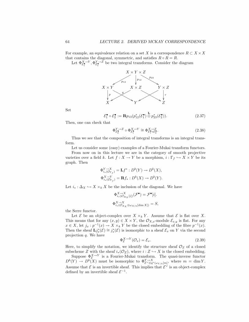
64 LECTURE 2. DERIVED MCKAY CORRESPONDENCE
For example, an equivalence relation on a set X is a correspondence R ⊂ X×Xthat contains the diagonal, symmetric, and satisfies R R = R.
Let ΦX→YE•1,ΦY→ZE•1
be two integral transforms. Consider the diagram
X × Y × Zp23
&&MMMMMMMMMMM
p12xxppppppppppp12
X × Y
p
q
&&NNNNNNNNNNNN X × Z
xxpppppppppppp
&&NNNNNNNNNNNN Y × Z
r
xxpppppppppppp
X Y Z
SetE•1 E•2 := Rp13(p∗12(E•1 )
L⊗ p∗23(E•2 )). (2.37)
Then, one can check that
ΦY→ZE•2 ΦX→YE•1∼= ΦX→ZE•1 E•2 . (2.38)
Thus we see that the composition of integral transforms is an integral trans-form.
Let us consider some (easy) examples of a Fourier-Mukai transform functors.From now on in this lecture we are in the category of smooth projective
varieties over a field k. Let f : X → Y be a morphism, i : Γf → X × Y be itsgraph. Then
ΦY→Xi∗(OΓf) = Lf∗ : Db(Y )→ Db(X),
ΦX→Yi∗(OΓf) = Rf∗ : Db(X)→ Db(Y ).
Let i∗ : ∆X → X ×k X be the inclusion of the diagonal. We have
ΦX→Xi∗(O∆X[i])(F
•) = F•[i].
ΦX→Xi∗(O∆X⊗ωX/k[dimX]) = S,
the Serre functor.Let E be an object-complex over X ×k Y . Assume that E is flat over X.
This means that for any (x, y) ∈ X × Y , the OX,x-module Ex,y is flat. For anyx ∈ X, let jx : p−1(x) → X ×k Y be the closed embedding of the fibre p−1(x).Then the sheaf Lj∗x(E) ∼= j∗x(E) is isomorphic to a sheaf Ex on Y via the secondprojection q. We have
ΦX→YE (Ox) = Ex. (2.39)
Here, to simplify the notation, we identify the structure sheaf OZ of a closedsubscheme Z with the sheaf i∗(OZ), where i : Z → X is the closed embedding.
Suppose ΦX→YE is a Fourier-Mukai transform. The quasi-inverse functorDb(Y ) → Db(X) must be isomorphic to ΦY→XE∨⊗q∗(ωY/k[m], where m = dimY .Assume that E is an invertible sheaf. This implies that E∨ is an object-complexdefined by an invertible sheaf E−1.
2.2. FOURIER-MUKAI TRANSFORM 65
Example 2.2.7. Let us take X = Y = E, where E is an elliptic curve over afield k. Let x0 ∈ E(k). Consider the invertible sheaf P = OE×E(−p−1(x0) −q−1(x0) + ∆E). Let
P = −p−1(x0)− q−1(x0) + ∆E .
It follows from (2.39), for any closed point x ∈ E,
ΦE→EP (Ox) ∼= OE(x− x0). (2.40)
Recall, that a choice of a point x0 ∈ E(k) defines an isomorphism of abeliangroups
E → Pic0(E), x 7→ OX(x− x0), (2.41)
where the group law on E is defined by x ⊕ y ∼ x + y − x0, where we use theRiemann-Roch Theorem and Serre’s duality that give
h0(OE(D)− h0(OE(−D)) = degD, (2.42)
giving in particular that h0(OE(x+y−x0)) = 1. Thus we see that the bijection(2.41) can be defined by the integral transform ΦP .
Let us us see that ΦP is a Fourier-Mukai transform. In fact, this exampleappears in the paper of Mukai, where the Fourier-Mukai transform was intro-duced.
Before doing this let us compute explicitly some of the transforms.We will use the following result from [Hartshorne[, Chap. III, Theorem
12.11) to compute the higher direct images of coherent sheaves. Let f : X → Ybe a projective morphism of noetherian schemes and F be a coherent sheaf onX, flat over Y . Suppose Ri+1f∗F is locally free, then
Rif∗F(y) := Rif∗F ⊗Y Spec k(y) ∼= Hi(Xy,Fy),
where Xy = f−1(y) is the scheme-theoretical fibre of f over y and Fy = F ⊗OX
OXy.
Let us apply this result to our morphism q : E × E → E and use thatR2f∗F = 0 because the relative dimension of q is equal to 1. We obtain that,for any coherent sheaf F on E × E, flat over E, we have
R1q∗(F)(y) ∼= H1(q−1(y),F|q−1(y)).
For any y ∈ E we have
P ⊗ p∗(OE(D)) ∼= OE×E(P + p∗(D)).
Hence
P ⊗ p∗(OE(D))|q−1(y) ∼= OE((P + p∗(D)) ∩ q−1(y)) = OE(D + y − x0).
Thus we obtain
R1q∗(P⊗p∗(OE(D))(x) = H1(E,OE(D+x−x0)) ∼= H0(E,OE(−D+x0−x)).
66 LECTURE 2. DERIVED MCKAY CORRESPONDENCE
Applying (2.42), this gives
R1q∗(P ⊗ p∗(OE(D))(x) = 0, if degD ≥ 0, D + x− x0 6∼ 0,
Assume D + x− x0 ∼ 0. Note that this can happen only for a unique point x.Then R1q∗(P ⊗ p∗(OE(D))(x) ∼= H1(E,OE) ∼= k, and we get
H1(ΦE→EP (OE(D))) = Ox,
H0(ΦE→EP (OE(D)))(y) = 0, y 6= x.
We have
H0(ΦE→EP (OE(D))(x) ∼= H0(E, q∗(OE×E(P + p∗(D)))
∼= H0(E × E,OE×E(P + p∗(D)).
Since degD = 0, using the intersection theory on the surface E × E, we get
(P + q∗(D))2 = P 2 + 2P · q∗(D) = (∆− p−1(x0)− q−1(x0))2 = −2 (2.43)
(we use that ∆2 = Eu(E) = 0). Since the canonical class of E×E is equal to 0,the adjunction formula gives C2 = 2h1(OC)− 2 for any irreducible curve C onE ×E. Since C projects surjectively to E, h1(OC) > 0. Thus C2 ≥ 0. SupposeH0(E × E,OE×E(P + p∗(D))) 6= 0, then P + p∗(D) is linearly equivalent toan effective divisor, and it follows from above that its self-intersection is non-negative. This contradiction with (2.43) shows that H0(E × E,OE×E(P +p∗(D))) = 0. Collecting all of this together we obtain
ΦE→EP (OE(D))) = Ox[−1] if D ∼ x0 − x. (2.44)
Comparing with (2.40), we find that
ΦE→EP ΦE→EP (Ox) = Ox[−1], (2.45)
where x means the negative of x in the group law on E.Now consider the distinguished triangle corresponding to the exact sequence
0→ OE(−x)→ OE → Ox → 0.
Applying ΦE→EP , we obtain the distinguished triangle
ΦE→EP (OE(−x))→ Ox0 [−1]→ OE(x− x0)→ ΦE→EP (OE(−x))[1].
It implies that
ΦE→EP (OE(−x)) ∼= Ox0 [−1]⊕OE(x− x0).
Finally, if F = O2x, then the extension
0→ Ox → O2x → Ox → 0
2.2. FOURIER-MUKAI TRANSFORM 67
implies that ΦE→EP (O2x) fits in the extension
0→ OE(x− x0)→ ΦE→EP (O2x)→ OE(x− x0)→ 0.
It corresponds to a non-trivial element in the space
Ext1E(OE(x− x0),OE(x− x0)) ∼= Ext1E(OE ,OE) ∼= H1(E,OE) ∼= k.
After these concrete computations, let us start proving that ΦE→EP is aFourier-Mukai transform. In fact, we will prove that
ΦE→EP ΦE→EP∼= ι∗ [−1], (2.46)
where ι : E → E is the automorphism of E defined by the negation automor-phism x→ x, and [−1] is the shift automorphism. This agrees with (2.45).
To prove (2.46), it suffices to prove that
P P ∼= OΓ(ι)[−1]. (2.47)
We will use the following well-known seesaw principle.
• Let f : X → Y be a smooth projective morphism of algebraic varietiesover a field k admitting a section s : Y → X. Assume that the functiony → dimk(y)H
i(Xy,OXy) is constant for any i ≥ 0. Let L and M be
invertible sheaves such that L|Xy∼=M|Xy for all closed points y ∈ Y and
s∗(L) ∼= s∗(M). Then L ∼=M.
To prove it consider the invertible sheaf N = L ⊗ M−1. For any closedpoint y ∈ Y we have an isomorphism N|Xy
∼= OXy . Since f is smooth,starting with Rdim f+1f∗(N ) = 0, we obtain that the fibres Rif∗N (y) are iso-morphic to Hi(Xy,Oy) and, by assumption, their dimension is independent ofy. This implies that the sheaves (Rif∗N )(y) are locally free of rank equal todimk(y)H
i(Xy,OXy). In particular, we obtain that the sheaf K = f∗(N ) is an
invertible sheaf on Y . Consider the homomorphism f∗f∗N → N . Restricting tofibres, we obtain an isomorphism. Thus N ∼= f∗(K). Now the second assump-tion on L,M implies that OY ∼= s∗(N ) ∼= s∗(f∗(K)) ∼= K. This gives N ∼= OXand hence L ∼=M.
We will apply the seesaw principle to the case when f : X×Y → Y is the pro-jection. Since all fibres are isomorphic, the assumption on dimk(y)H
i(Xy,OXy)
is obviously satisfied. Note that the assumption is always satisfied if k = C.
Consider the addition map
µ : E × E → E, (x, y) 7→ x⊕ y.
We have µ−1(z)|q−1(x) = z x, and the same is true for another projection.Restricting the divisor µ−1(x)− µ−1(x0) to fibres of p and q, and applying theseesaw principle to any of the two projections E × E → E, we easily obtain
µ−1(x)− µ−1(x0) ∼= p∗(OE(x− x0))⊗ q∗(OE(x− x0)).
68 LECTURE 2. DERIVED MCKAY CORRESPONDENCE
Now, using this, we make similar comparison and the seesaw principle to obtainan isomorphism
p∗12(P)⊗ p∗13(P) ∼= π∗(P),
whereπ : E × E × E → E × E, (x, y, z) 7→ (y, x+ z).
This impliesP P ∼= Rp13∗(π∗(P)).
Applying the base-change formula for higher direct images (see [Hartshorne],Chap. III, §9) to the Cartesian diagram
E × E × E π //
p12
E × Eq
E × E
µ // E
we find thatRp13∗(π∗(P)) ∼= µ∗(Rq∗(P)).
By our previous computations (2.44), we have
Rq∗(P) ∼= ΦE→EP (OE) ∼= Ox0 [−1].
This givesP P ∼= µ∗(Ox0 [−1]) = OΓ(ι)[−1].
This checks (2.47).
Recall that any abelian category A defines the Grothendieck group K(A).By definition
K(A) = ZOb(A)/H,
where H is the subgroup generated by elements C − A − B = 0, where 0 →A→ C → B → 0 is an exact sequence in A. The canonical map Ob(A)→ K(A)has the following universality property: any function χ on Ob(A) satisfyingχ(C) = χ(A) + χ(B) for any exact sequence as above, extends to a uniquefunction on K(A). We denote by [X] the image of an object X of A in K(A).
Since Cpb(A) is an abelian category, we can define K0(Cpb(A)). Consideringthe inclusion functor A → Cpb(A) and applying the universality property ofK(A), we obtain a homomorphism of groups φ : K(A) → K(Cpb(A)). Definethe homomorphism K(Cpb(A))→ K(A) by sending [X•] to
∑i(−1)i[Xi]. It is
checked that this is well-defined and is equal to the inverse of φ. Notice that[X•[1]] = −[X•].
Next consider the categories Kb(A) and Db(A). We define K(K(A)) =ZOb(K(A)/H, where H is generated by C• − A• − B• whenever we have a dis-tinguished triangle A• → C• → B• → A•[1]. Similar definition is given forK(Db(A)). It is immediately checked that [X•[1]] = −[X•] (consider the zeromap X• → 0 and take the corresponding distinguished triangle, its cone is
2.2. FOURIER-MUKAI TRANSFORM 69
X•[1]). Also an exact sequence of complexes in Cpb(A) defines a distinguishedtriangle, so that this definition agrees with the definition of K(Cpb(A)) in thesense that the universality property of K defines a unique homomorphism ofgroups K(A) ∼= K(Cpb(A))→ K(Kb(A)). The exact sequences in Cpb(A))
0→ ker(d)→ X• → im(d)→ 0,
0→ im(d)[−1]→ ker(d)→ H → 0
yield[H•] = [X•].
This shows that the image of quasi-isomorphic complexes inK(Kb(A)) are equal.This shows that
K(Db(A)) ∼= K(Kb(A)).
Also the exact sequences of object-complexes
0→ ker(di)→ Xi → im(di)→ 0,
0→ im(di−1)→ ker(di)→ Hi → 0
give∑i(−1)i[Xi] =
∑i(−1)[Hi]. Since H• =
∑iH
i[−i], we obtain
[X•] = [H•] =∑i
[Hi[−i]] =∑i
(−1)i[Hi] =∑i
(−1)i[Xi]. (2.48)
The map Ob(Kb(A)) → K(A) sending X• →∑i(−1)i[Xi] factors through
K(Kb(A)) and defines the inverse of the map K(A) → K(Kb(A)). Thus wehave
K(Db(A)) ∼= K(Kb(A)) ∼= K(A).
Note how everything agrees with finite resolution complexes K•. We have
[H0(K•)] = [K•] =∑i
(−1)[Ki].
We setK0(X) = K(Coh(X)), K0(X) = K(Qcoh(X))
AssumeX is a smooth projective variety. By taking finite locally free resolutionsPF of objects of coh(X) we can define the ring structure on K0(X) by
[F ][G] = [PF ⊗ PG ],
and then, extending to any complexes, to get
[F•] · [G•] = [FL⊗ G].
The assignment X → Db(X) → K0(X) defines a fibred functor on the fi-bred category X → Db(X), where we take K0(f∗) := f∗ to be defined by
70 LECTURE 2. DERIVED MCKAY CORRESPONDENCE
[F•] → [f∗(F•)]. Also the same assignment defines a cofibred functor if weset K0(f∗) := f! to be defined by [F ] → [Rf∗(F•)]. Thus we can combine itwith the categorical integral transform ΦY→XP by taking K = ·[P], to obtainthe K-theoretic integral transform
[Φ]K,Y→X[P] : K0(Y )→ K0(X), [Φ]K,X→Y[P] : K0(X)→ K0(Y )
such that the diagram
Db(Y )ΦY→XP //
[?]
Db(X)
[?]
K0(Y )
[Φ]Y→XP // K0(X)
is commutative.Finally we can extend Example 2.2.3 to our situation. Let PAVsm/C be the
category of smooth projective varieties over k. We take the functors
F : (PAVsm/C)op → Mod(F), X → H∗(X,F),
G : PAVsm/C→ Mod(F), X → H∗(X,F),
where F = Z,Q,R, or C. For any morphism f : X → Y we have F (f) =f∗ : H∗(Y ) → H∗(X) and G(f) := f∗ is defined by using the Poincare dualityH∗(X) → H2 dimX−∗ on X, then composing it with f∗ : H2 dimX−∗(X) →H2 dimY−∗(Y ) and using the Poincare duality again H2 dimY−∗(Y ) ∼= H∗(Y ).
For any cohomology class α ∈ H∗(X×Y ), we define the kernel Kα : H∗(X×Y ) → H∗(X × Y ) as the cup-product with α. This defines the cohomologicalintegral transform
ΦH,Y→Xα : H∗(Y )→ H∗(X), ΦH,X→Yα : H∗(X)→ H∗(Y ).
We also take K : H∗(X × Y,F) → H2n+2m−∗(X × Y,F) to be the Poincare-duality map, and q∗ : H2n+2m−∗(X × Y,F) → H2n−∗(X × Y,F) and composeit with the Poincare duality H2n−∗(X × Y,F) → H∗(X,F) on X to obtain acofibred functor f∗ : H∗(X,F)→ H∗(Y,Q).
Next recall the Grothendieck-Riemann-Roch Theorem (see [Hartshorne], Ap.A, §4).
Theorem 2.2.8. There exists a homomorphism of abelian groups ch : K0(X)→H∗(X,Q) such that for any e ∈ K0(X),
ch(f!(e)) · td(Y ) = f∗(ch(e) · td(X)).
Here, ch(e) and td(X), td(Y ) are defined as follows (see [Hartshorne], Ap-pendix 4). For any locally-free sheaf of rank r, we write (formally) the Chernpolynomial ct(E) in the form
ct(E) = 1 +r∑i=1
ci(E)ti =r∏i=1
(1 + ait).
2.2. FOURIER-MUKAI TRANSFORM 71
It follows from the definition that ct(E) depends only on e = [E ] ∈ K0(X). Weput
ch(E) =r∑i=1
eai , td(E) =r∏i=1
ai1− e−ai
wherex
1− e−x= 1 +
12x+
112x2 − 1
720x4 + · · · .
(all operations are taken in the cohomology rings). We set td(X) = td(TX),where TX is the tangent sheaf of X. Since any coherent sheaf has a locally freeresolution, we can extend the definition of ch(e) to any e ∈ K0(X).
For any complex E• ∈ Db(X) we have
e = [E•] =∑i
(−1)i[Hi(E•)] =∑i
(−1)i[Hi(E i)].
Soch(E•) = ch([E•]) =
∑i
(−1)ich(Hi(E•)) =∑i
(−1)ich(E i).
In this way we extend the Grothenidieck-Riemann-Roch formula to complexes.
Remark 2.2.9. One can extend everything to the case of nonsingular projec-tive varieties over any field k. To do this one replaces the cohomology ringwith the Chow ring A∗(X) of algebraic cycles modulo rational equivalence (see[Hartshorne], Appendix A, [Fulton]).
Definition 2.2.2. The Mukai vector of a class e ∈ K0(X) is defined to be thecohomology class
Mu(e) = ch(e) ·√
td(X).
We setMu(E•) := v([E•]).
With this definition we have the following.
Theorem 2.2.10. For any e ∈ K0(X × Y ) and a ∈ K0(Y ), we have
ΦH,Y→XMu(e) (Mu(a)) = Mu(ΦK0,Y→Xe (a)).
Proof. Consider the commutative diagram
K0(Y )q∗ //
Mu
K0(X × Y ) ·e //
Mu√p∗(td(X))
−1
K0(X × Y )p! //
Mu√q∗(td(Y ))
K(X)
Mu
H∗(Y )
q∗ // H∗(X × Y )·Mu(e)// H∗(X × Y )
p∗ // H∗(X)
To check the commutativity of the first square, we use that
td(X × Y ) = p∗(td(X)) · q∗(td(Y ))
72 LECTURE 2. DERIVED MCKAY CORRESPONDENCE
because TX×Y ) ∼= p∗(TX)⊕ q∗(TY ) and the Todd class of the direct sum is theproduct, i.e. td(E ⊕F) = td(E) ·td(F). The commutativity of the second squareuses the same and the multiplicativity property of ch, i.e. ch(x.y) = ch(x)ch(y).The commutativity of the third square is the GRR Theorem applied to theprojection p.
In the special case when Y = Spec C, the Grothendieck-Riemann-RochTheorem gives the Hirzebruch-Riemann-Roch formula
χ(F) :=dimX∑i=0
(−1)q dimkHq(X,F) =
∫X
ch([F ]) · td(X),
where the integral means taking the projection to H2 dimX(X,Q). We statedit for object-complexes only. But, it is immediately extended to complexes byadditivity
χ(F•) =∑i
(−1)iχ(F i), χ([F•]) =∑i
(−1)iχ([F i]).
If F is a coherent sheaf, we take its locally free resolution R•, and apply theformula to the complex R• by first computing the Chern polynomial. Note thattaking F = OX , we get
χ(X,OX) =∫X
td(X) =
1− g if,dimX = 1c2X+c2(X)
12 if dimX = 2c1(X)c2(X)
24 if dimX = 3.
(2.49)
Example 2.2.11. Assume X is a curve of genus g. By Corollary 2.1.13, anycomplex is isomorphic in the derived category to the direct sum of twistedobject-complexes. We know that [F•[i]] = (−1)i[F•]. So χ(F•[i]) = (−1)iχ(F•)and ch(F•[i]) = (−1)ich(F•), so we need only to compute χ(F), where F iseither a locally free sheaf or a torsion sheaf. We have H∗(X,Z) = H0(X,Z) ⊕H2(X,Z) = Z ⊕ Z. Any closed point x defines its fundamental cycle [x] ∈H2(X,Z) that we can identify with number 1. By additivity, this assigns toany divisor D =
∑nixi its fundamental class [D] ∈ H2(X,Z) identified with
deg(D). We have
c1(OX(D)) = degD, ch(OX(D)) = [X] + deg(D),
td(X) = [X] +12
degKX = [X] + 1− g.
Any locally free sheaf E of rank r fits in an exact sequence of locally free sheaves
0→ E1 → E → E2 → 0 (2.50)
where rank(E1) = 1, rank(E2) = r − 1. In fact we first tensor E with someOX(D) with degD >> 0 to assume that E has a section. This defines an
2.2. FOURIER-MUKAI TRANSFORM 73
injective homomorphism of sheaves OX → E ⊗ OX(D). Then we untwist bytensoring with OX(−D) to obtain an injection OX(−D)→ E . Then we saturatethis injection, by taking the largest invertible subsheaf of E that contains OX(D)such that the quotient sheaf has no torsion, hence locally free. By using locallyfree resolutions, we obtain that K0(X) is generated by the classes [OX(D)] ofinvertible sheaves.
We can do better. Consider the map
det : K0(X)→ Pic(X), E → det(E) := ΛrankE(E),
where E is a locally free sheaf, and we use that K0(X) is generated by theclasses of those. An exact sequence (2.50) of locally free sheaves gives det(E) =det(E1) ⊗ det(E2). This shows that the map is well-defined and is a homomor-phism of abelian groups. Consider the map
α : K0(X)→ Z⊕ Pic(X), E → (rank(E),det(E)).
It is obviously a surjective map. It is not a trivial fact that α is an isomorphism.In fact, this homomorphism is defined for varieties of any dimension, and itskernel is isomorphic to F 2(K0(X)), where F i(K0(X)) is the subgroup generatedby the classes of sheaves with support in a closed subscheme of codimension ≥ i(see [Manin, Russ. Math. Survey, 1969).
In the case when E is locally free, the Riemann-Roch gives
χ(X, E) = deg det(E) + rank(E)(1− g).
For any two complexes F•,G• ∈ Ob(Db(X)) define
χ(F•,G•) =∑i
(−1)i dimk Extik(F•,G•) = χ(F∨L⊗ G•).
Define the Mukai pairing on H∗(X,Q) by
〈v, v′〉X =∫X
exp(c1(X)/2) · v∨ · v′,
where, for any v =∑vs ∈ ⊕H2s(X,Q), we set v∨ =
∑s(−1)svs.
Proposition 2.2.12.
χ(F•,G•) = 〈Mu(E•),Mu(G•)〉.
Proof. By Riemann-Roch,
χ(F•,G•) = χ(F•∨L⊗ G•) =
∫X
ch(E•∨) · ch(F•) · td(X) (2.51)
=∫X
(ch(E•∨) ·√
td(X)) · (ch(F•) ·√
td(X)).
74 LECTURE 2. DERIVED MCKAY CORRESPONDENCE
If ct(F•) =∏
(1 + ait), then ch(F•∨) =∏
(1 − ait). This gives ch(F•) =∑i e−ai = ch(E•)∨. Now it is easy to see that
td(X)∨ · exp(c1(X)) =∏ −γi
1− eγi·∏
eγi ,
where ct(TX) =∏i(1 + γit
i). Thus we can rewrite (2.51) in the form
χ(F•,G•) =∫X
exp(c1(X)/2) ·Mu(F•)∨ ·Mu(G•).
This proves the assertion.
Example 2.2.13. Assume dimX = 1. Let v = v0 + v1 ∈ H∗(X). Then v∨ =v0−v1 and td(X) = [X]+td(X)1,
√td(X) = [X]+ 1
2 td1. Let f = [F•], g = [G•],then
χ(F•,G•) = 〈Mu(f)∨,Mu(g)〉
=∫X
([X] + (1− g))(ch0(f)− ch1(f)(ch0(g) + ch1(g)([X]− 12td1)([X] +
12td1)
= ch(f)0ch(g)0(1− g) + ch(f)ch1(g)− ch(g)ch(f))1
= rank(E•)rank(G•)(1− g) + rank(F•) deg det(G•)− rank(G•) deg(det(F•)).
Hererank[K•] =
∑i
(−1)irankKi =∑i
(−1)irankHi(K•),
and the rank of a coherent sheaf is equal to the dimension of its stalk at thegeneral point η over k(η).
Example 2.2.14. Let F• = G• = E , where E is an object-complex correspond-ing to a locally free sheaf of rank r. We get
χ(E , E) = χ(E∨ ⊗ E) = Mu(E)2 := 〈Mu(E),Mu(E)〉.
We have dimH0(E∨ ⊗ E) = dimk Endk(E). A locally free sheaf (or the corre-sponding vector bundle) is called simple if Endk(E) = k. Using the deformationtheory one can show that m = dimH1(X, E∨ ⊗ E) is equal to the dimension ofthe moduli space of simple vector bundles at the point corresponding to E . IfdimX = 1, we get the formula
m = rank(E)2(g − 1) + 1.
In the case rank(E) = 1, we obtain m = g = dim Picd(X), where d = deg(E).If dimX = 2 and ωX ∼= OX (i.e. X is an abelian surface or a K3 surface),
we can use the Serre duality, to obtain dimH2(X, E∨ ⊗ E) = dim End(E). Thisgives the formula
m = 2−Mu(E)2.
2.3. EQUIVARIANT DERIVED CATEGORIES 75
In particular, simple bundles which are rigid, i.e. m = 0, satisfy Mu(E) = 2.For example, let rank E = r, ci(E) = ci. We have ch(E) = r + c1(E) + 1
2c21 − c2,
td(X)1 = 0, td(X)2 = χ(X,OX),√
td(X) = 1 + 12χ(X,OX). This gives
Mu(E) = (Mu(E)0,Mu(E)1,Mu(E)2) = (r, c1(E),12(rχ(X,OX) + c21)− c2),
Mu(E)2 = (r − 1)c21 − 2rc2 + r2χ(X,OX). (2.52)
Assume r = 1. We get Mu(E)2 = 0 if X is an abelian surface, so that m = 2,and Mu(E)2 = 2 if X is a K3 surface, so that m = 0.
Remark 2.2.15. For a K3 surface X one defines the Mukai lattice by Mu(X) =H0(X,Z)⊕ Pic(X)⊕H4(X,Z) with inner product
(a, b, c) · (a′, b′, c′)〉 = b · b′ − a′ · c− a′ · c.
We have〈Mu(e),Mu(e′)〉X = −Mu(e) ·Mu(e′).
2.3 Equivariant derived categories
Let C be a category and G be a group object in C, i.e. a Gr-object in C, whereGr is the category of groups (see section 1.1). For any S ∈ Ob(C), the setG(S) := hG(S) = MorC(S,G) is a group and, for any morphism S′ → S inC, the maps G(S) → G(S′) are homomorphism of groups. Assume that C hasproducts and the functor S → eG(S) ⊂ G(S), where eG(S) is the neutralelement in G(S), is represented by a final object e in C. By Yoneda’s Lemma,there is a morphism µ : G×G→ G (the group law) such that, for any S ∈ Ob(C),the map of sets µ(S) : G(S) × G(S) → G(S) is a group law on the set G(S).There is a morphism ε : e→ G defined by he(S)→ G(S) with the image equal toeG(S). Also there is morphism ι : G→ G with G(S)→ G(S) expressing takingthe inverse. The morphisms µ, ε, ι must satisfy certain natural commutativediagrams describing the group axioms.
An action of G on X ∈ Ob(C) is a morphism σ : G×X → X such that thecorresponding map of pre-sheeaves hG×hX → hX is an action in the category ofpresheaves. For any S ∈ C we have a group action σ(S) : G(S)×X(S)→ X(S)in the category of sets, where X(S) = hX(S). These actions must be functorialin S. For any g, h ∈ G(S), x ∈ X(S) we write g·h = µ(S)(g, h), g·x = σ(S)(g, x).
Let (X,σ) be a pair consisting of an object X and a G-action σ : G×X → X.A G-equivariant morphism (X,σ) → (X ′, σ′) is a morphism f : X → X ′ suchthat the diagram
G×X σ //
idG×f
X
f
G×X ′ σ′ // X ′
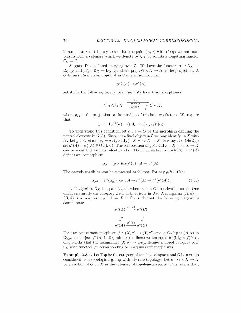
76 LECTURE 2. DERIVED MCKAY CORRESPONDENCE
is commutative. It is easy to see that the pairs (A, σ) with G-equivariant mor-phisms form a category which we denote by CG. It admits a forgetting functorCG → C.
Suppose D is a fibred category over C. We have the functors σ∗ : DX →DG×X and pr∗X : DX → DX×G, where prX : G ×X → X is the projection. AG-linearization on an object A in DX is an isomorphism
pr∗X(A)→ σ∗(A)
satisfying the following cocycle condition. We have three morphisms
G×G×XtidG×σ //
tp23 //
µ×idX // G×X,
where p23 is the projection to the product of the last two factors. We requirethat
(µ× idX)∗(α) = ((idG × σ) p12)∗(α).
To understand this condition, let α : e → G be the morphism defining theneutral elements inG(S). Since e is a final object in C we may identify e×X withX. Let g ∈ G(e) and σg = σ(g×idX) : X = e×X → X. For any A ∈ Ob(DX)set g∗(A) = σ∗g(A) ∈ Ob(DX). The composition prX(g×idX) : X = e×X → Xcan be identified with the identity idX . The linearization α : pr∗X(A)→ σ∗(A)defines an isomorphism
αg = (g × idX)∗(σ) : A→ g∗(A).
The cocycle condition can be expressed as follows. For any g, h ∈ G(e)
αg·h = h∗(αg) αh : A→ h∗(A)→ h∗(g∗(A)). (2.53)
A G-object in DX is a pair (A,α), where α is a G-linearization on A. Onedefines naturally the category DX,σ of G-objects in DX . A morphism (A,α)→(B, β) is a morphism φ : A → B in DX such that the following diagram iscommutative
σ∗(A)σ∗(φ) //
α
σ∗(B)
β
q∗(A)
q∗(φ) // q∗(B)
For any equivariant morphism f : (X,σ) → (Y, σ′) and a G-object (A,α) inDY,σ, the object f∗(A) in DX admits the linearization equal to (idG × f)∗(α).One checks that the assignment (X,σ) → DX,σ defines a fibred category overCG with functors f∗ corresponding to G-equivaraint morphisms.
Example 2.3.1. Let Top be the category of topological spaces andG be a groupconsidered as a topological group with discrete topology. Let σ : G ×X → Xbe an action of G on X in the category of topological spaces. This means that,
2.3. EQUIVARIANT DERIVED CATEGORIES 77
for any g ∈ G, the map g : X → X,x → g · x, is continuous. Let Shab be thefibred category over Top that assigns to each X the category Shab
X of abeliansheaves on X with the pull-back functors f∗. As above we form the categoryTopG of topological spaces with an action of the group G and consider thefibred category X → Shab
G (X) of G-linearized abelian sheaves, or just abelianG-sheaves. Taking for the final object e in Top a singleton e, we see that a G-linearization is defined by isomorphisms αg : A → g∗(A) satisfying the cocyclecondition (2.53).
One can also express the linearization as follows. Recall the original defini-tion of a sheaf F in terms of its espace etale. It is a topological space Es(F)which, as a set, is equal to the union
∐x∈X Fx of stalks. It comes with the
projection Es(F)→ X by sending Fx to x. We equip the set with the strongesttopology such that all local sections s : U → Es(F) defined by s → sx ∈ Fxare continuous maps. In this way F is reconstructed from Es(F) by expressingF(U) as the set of all continuous sections U → Es(F). Now one can check thata G-linearization on F is a lift of the action of G on X to Es(F) compatiblewith the projection.
Recall that a morphism of ringed spaces (X,OX) → (Y,OY ) consists of acontinuous map f : X → Y and a map of sheaves f# : OY → f∗OX . Weconsider a group G as a discrete topological space with the constant sheaf ofrings ZG. The product (G,ZG) × (X,OX) can be identified with the disjointsum
∐g∈GXg of copies of X together with the sheaf of ring equal to OX on each
component Xg. An action of G on (X,OX) consists of an action G×X → X inthe category Top together with a morphism of sheaves σ# : OX → σ∗(OG×X).It is easy to see that it is defined by a collection of automorphisms g : (X,OX)→(X,OX) satisfying the cocycle condition. By definition of a morphism of ringedspace, for any open subset U ⊂ X, there is an isomorphism of rings g∗OX(U)→OX(g−1(U)), these isomorphisms must define a G-linearization on the sheafOX .
This defines a category RTopG whose objects are ringed topological spacestogether with a G-action. Now we can consider a fibred category over RTopG byassigning to each (X,OX) the category ModG(OX) of G-linearized OX -modules.We call its objects G−OX -modules.
For example, suppose G acts trivially on X and on OX . Then a G − OX -module is defined by a set of isomorphisms αg : A → g∗(A) = A of OX -modulessuch that αg·g′ = αg αg′ . In other words it defines a homomorphism of groupsG → AutOX
(A), g → αg. Specialing more, we take for X a point so thatOX is a ring R and A is a R-module M . Then a G − OX -module becomes arepresentation of G in M , i.e. a homomorphism G→ AutR(M).
More generally, suppose G acts trivially on X but not necessary triviallyon OX . We can define a new sheaf of rings OX#G whose sections on an opensubset U is the skew group algebra OX(U)#G. Recall that for any ring R witha group action G → Aut(R), (g, r) 7→ gr, one defines the skew group algebraR#G. It is the free abelian group RG of formal linear combinations
∑g∈G rgg
with product defined by
(rg · g)(rg′g′) = rggrg′gg
′.
78 LECTURE 2. DERIVED MCKAY CORRESPONDENCE
One can show that ModG(OX) is equivalent to the category Mod(OX#G).It is easy to check that the category ofG−OX -modules is an abelian category.
It also has enough of injective objects. Here is the proof due to A. Grothendieck.Let Mx be a collection of OX,x-modules for all x ∈ X. It defines a sheaf
by setting M(U) =∏x∈U Mx. In other words M =
∏x∈X(ix)∗Mx, where
ix : x → X is the inclusion map and Mx is the sheaf on x with value Mx. Forany OX -module F a map of F toM is defined by a family of homomorphismsFx → Mx, x ∈ X. Let Y = X/G be the set of orbits of G. For each x ∈ Xlet Ux = OX,x#Gx, where Gx is the stabilizer of x. For each y ∈ Y choosea representative ξ(y) ∈ G · x and let Uy = Uξ(y). Define the sheaf of algebrasU =
∏y∈Y (iy)∗(Uy). Let A be the sheaf defined by a collection (Ay)y∈Y of
Uy-modules. Now define a G−OX -sheaf A on X by the collection of modulesAx = Ay where x = g(ξ(y)). The group G acts naturally on A via its naturalaction on Es(A). For any G − OX -sheaf M on X let M be the sheaf of U-modules defined by the Uy-modules Mξ(y). Then
HomU (M,A) = HomOX(M, A).
Indeed an element in the first set is defined by a collection of homomorphismsMx → Ax = gAξ(y) which is determined uniquely by homomorphismsMξ(y) →Ay.
Now it remains to take A to be defined by a collection of injective Ux-modules. The corresponding sheaf A is an injective G-sheaf of OX -modules.Since Mod(U) has enough injective modules, we can embed M in an injectiveA, to get an embedding ofM in an injective OX -module A.
Let S = Sch/k be the category of schemes over a field k. A group object Gin Sch/k is called a group scheme over k. Consider the fibred category X →Qcoh(X). Let σ : G × X → X be an action. For any field extension K/k wehave an action GK×XK → XK , where the subscript denotes the base extension.Now an element g ∈ G(K) defines an automorphism g : XK → XK and thefunctor g∗ : Qcoh(XK) → Qcoh(XK). A G-object in Qcoh(X) is a sheaf Fsuch that for all K/k there is an isomorphism αg : FK → g∗(FK) satisfying thecocycle condition. These isomorphisms should be compatible with compositionof extensions.
From now on we will restrict ourselves with the special case when S is thecategory AV/k of algebraic varieties over a field k and G a finite group, con-sidered as a constant group scheme over k (i.e. the Yoneda functor hG is theconstant presheaf with values equal to G). In this case the action of G onX is determined by a homomorphism G → Autk(X). A linearization on aquasi-coherent sheaf F is a family of isomorphisms of sheaves αg : F → g∗(F)satisfying the cocycle condition. Let QcohG(X) be the category of G-linearizedquasi-coherent sheaves.
Example 2.3.2. Suppose E is a G-linearized locally free sheaf of rank r ona scheme X over a field k. Let V(E) = Spec Sym•(E∨) be the corresponding
2.3. EQUIVARIANT DERIVED CATEGORIES 79
vector bundle. The sheaf of local sections of V(E) is isomorphic to E . A G-linearization defines isomorphisms αg : E → g∗(E), and hence their transposesg∗(E)∨ = g∗(E∨)→ E∨. Taking the symmetric powers we obtain isomorphismsg∗(Sym•(E∨)) → Sym•(E∨) which define isomorphisms of vector bundles αg :g∗(V(E)) = X ×X V(E)→ V(E), the base change with respect to the morphismg : X → X. For each point x ∈ X the morphism αg defines a k(x)-linearisomorphism of the fibres V(E)g−1(x) → V(E)x. Thus a G-linearization on Eallows one to lift the action of G on X to the action of G on V(E), compatiblewith the natural projection morphism V(E)→ X. The converse is also true.
Example 2.3.3. LetX be an integral scheme with an action of a constant groupscheme G. Let Pic(X) be the group of isomorphism classes of invertible sheaveson X, or, equivalently the group of Cartier divisors modulo principal divisors.Let L = OX(D) be the invertible sheaf defined by a Cartier divisor D on X.The group G acts naturally on the constant sheaf k(X) of rational functionson X. We denote the action by f → gf . If f is considered as a morphism toP1, then gf = f g−1. Via the action of G on k(X)∗, the group G acts on thegroup of Cartier divisors CDiv(X) = Γ(k(X)∗/O∗X) (by transforming the localequation φ = 0 on U into the local equation gφ = 0 on g−1(U)).
Suppose D is a G-invariant divisor, i.e. g∗(D) = D (considered as a sectionsof k(X)∗/O∗X). Then OX(D)(U) = f ∈ k(X)∗ : fDU ∈ OX(U)/OX(U)∗.Thus f → gf defines an isomorphism OX(D)(U) → OX(D)(g−1(U)), f → gf .These isomorphisms define a linearization αg : g∗(OX(D)) → OX(D). Thisdefines a homomorphism from the group Div(X)G ofG-invariant Cartier divisorsto the group PicG(X) of isomorphism classes G-linearized invertible sheaves.An element of the kernel corresponds to a principal G-invariant Cartier divisorD = div(f). The function f must satisfy div(gf) = div(f) and hence satisfygf = cgf , where cg ∈ OX(X)∗ is an invertible global section of OX . Theassignment g → cg defines a homomorphism of groups χ : G → OX(X)∗.It is clear that OX(D) belongs to the kernel of the forgetting homomorphismr : PicG(X) → Pic(X). Although as an element of PicG(X) it is trivial if andonly if χ is the trivial homomorphism. In this case D = div(f), where f is aG-invariant section of k(X)∗.
Now start with any G-linearized invertible sheaf L defining an element ofPicG(X). Choose an isomorphism L ∼= OX(D) for some Cartier divisor Dand transfer the linearization to OX(D). An isomorphism αg : g∗(OX(D)) →OX(D) is defined by a rational function fg such that D+div(fg) = g∗(D). Thecocycle condition implies that fg′g = gfg′fg for any g, g′ ∈ G. In other wordsthe collection fgg∈G is a 1-cocycle of G with values in k(X)∗. If we considerk(X) as a Galois extension of its field of invariants k(X)G with the Galois groupG, then the famous Hilbert’s Theorem 90 implies that H1(G, k(X)∗) = 0. Thuswe can write fg = ga/a for some a ∈ k(X)∗ independent of g. Replacing D withD′ = D − div(a), we obtain g∗(D′) = D′ for any g ∈ G. Thus L is isomorphicas a G-sheaf to a sheaf OX(D) corresponding to G-invariant divisor.
To sum up we obtain that PicG(X) is isomorphic to the group of G-invariant
80 LECTURE 2. DERIVED MCKAY CORRESPONDENCE
divisors modulo principal divisors. We have an exact sequence
0→ Hom(G,OX(X)∗)→ PicG(X) r→ PicG(X)→ H2(G,OX(X)∗).
One can prove that the last homomorphism is surjective when X is a smoothprojective curve.
Let us specialize. Take X to be a smooth projective curve over an alge-braically closed field k. A Cartier divisor D can be identified with a Weil divisorD =
∑x nxx. It is G-invariant if the function x → nx is constant on G-orbits.
Thus any G-invariant divisor is an integral linear combination of orbits. Letπ : X → Y = X/G be the projection to the orbit space (which is a smoothprojective curve). A G-invariant principal divisor is a linear combination ofscheme-theoretical fibres of π. Let y1, . . . , yr be the orders with non-trivial sta-bilizers of orders e1, . . . , en. Assume Y = P1. Let PicG(X)0 be the subgroupof isomorphism classes of G-linearized invertible sheaves of degree 0. It is equalto the kernel of the homomorphism deg : PicG(X) → Z defined by the degreeof a divisor. The image of PicG(X) under this homomorphism is equal to acyclic group (m). Since the canonical sheaf ωX admits a G-linearization (thecorresponding G-invariant divisor can be defined by using the Hurwitz formulaKX = π∗(KP1) + R, where R =
∑diyi is the ramification divisor), we have
m|2g − 2.By above any element of PicG(X) is represented by a sum D =
∑nyy,
where y ∈ Y is considered as an effective divisor on X representing the orbitdefined by y. For any y 6∈ y1, . . . , yn, we can find a rational function f onP1 such that y − e1y1 = div(f). This shows that that we may represent anelement of PicG(X)0 by a linear combination
∑niyi with
∑ni = 0. Its kernel
consists of linear combinations∑mieiyi, where
∑mi = 0. This defines a
natural isomorphismPicG(X)0 → A(e1, . . . , er),
where A(e1, . . . , er) is the abelian group defined by generators g1, . . . , gr andrelations g1 + . . .+ gr = 0, eigi = 0, i = 1, . . . , r. Using the theory of elementarydivisors in the theory of abelian groups, we obtain
A(e1, . . . , er) ∼= Z/a1Z⊕ . . .⊕ Z/arZ,
where ai = ci/ci−1, c0 = 1, and
ck = g.c.d.((ei1 · · · eik)1≤i1<···<ik≤r), k = 1, . . . , r − 1.
For example, if g.c.d.(e1, . . . , er) = 1 we get PicG(X)0 = 0. On the otherhand, let X = P1 and G = Z/2Z that acts by (t0 : t1)→ (−t0, t1). We assumethat char(k) 6= 2. The exceptional orbits are 0 = (1 : 0) and ∞ = (0 : 1) withe1 = e2 = 2. A field of invariant rational functions is equal to k(x2), wherex = t1/t0. Thus we see that OX admits two non-isomorphic linearizationscorresponding to the divisors D = 0 −∞ and D = 0. They correspond to thegroup of characters Hom(Z/2Z, k∗) ∼= Z/2Z. Every sheaf OX(n) admits twonon-isomorphic linearizations corresponding to the divisors n·0 and (n+1)·0−∞.
2.3. EQUIVARIANT DERIVED CATEGORIES 81
Lemma 2.3.4. Let G be a group scheme. The category QcohG(X) is an abeliancategory. If G is a constant group scheme then QcohG(X) has enough injectiveobjects.
Proof. Let σ : G × X → X be the action. It is equal to the composition ofthe morphisms prX (idG, σ) : G × X → G × X → X. The first morphismis an automorphism and the second map is a flat morphism. Thus σ is a flatmorphism. This implies that σ∗, q∗ are exact functors. Let K = ker(F → G)be the kernel of a morphism of G-bundles. Then σ∗(K) = ker(σ∗(F)→ σ∗(G)),q∗(K) = ker(q∗(F) → q∗(G)) and the isomorphisms α : σ∗(F) → q∗(F), β =σ∗(G) → q∗(G) restrict to an isomorphism σ∗(K) → q∗(K) defining a lineariza-tion on K. Similarly we prove that the cokernels exist in QcohG(X).
The statement about sufficiently many injective objects follows from theprevious example. It is easy to see that the injective sheaves of modules weused are quasi-coherent.
Example 2.3.5. Assume X = Spec A and G = Spec O(G) are affine schemes.An action of G on X is defined by a structure of a Hopf algebra on A. It is agroup object in the dual category. In particular, it comes with a homomorphismµ# : O(G)→ O(G)⊗O(G) defining the group law on G and a homomorphismσ# : A→ O(G)⊗A defining the action onX. For any ringK and x ∈ X(K), g ∈G(K), we have µ(g, x) is defined by a homomorphism A → O(G) ⊗ A
g⊗x−→K ⊗K → K, where the last homomorphism is the multiplication. Assume Gis a constant affine group scheme defined by an abstract group G. This meansthat O(G) = ZG with multiplication law of functions. An action of G on Xis defined by a homomorphism of groups φ : G → Aut(A). In terms µ# thisis defined by the homomorphism A → O(G) ⊗ A = AG, a → fa : g → ga,where φ(g)(a) = ga. For any A-module M let gM denote the A-module Mwith scalar multiplication defined by a ·m = gm. Let gA be the structure of anA-algebra on A defined by the homomorphism of rings A→ A, a→ gaA. ThengM ∼= M ⊗A gA. Geometrically, gM∼ ∼= g∗(M∼), where g : SpecA → SpecAdefined by the homomorphism of algebras A→ gA.
A G-linearization onM consists of a collection of isomorphisms of A-modulesαg : M → gM . Note that, for any g ∈ G, a ∈ A,m ∈ M , we have αg(am) =gaαg(m). For any h ∈ G the automorphisms αh defines the automorphismgM → hgM which we denote by g∗(αh). The collection of automorphisms αgmust satisfy the cocycle condition αgh = h∗(αg) αh.
Let A#G be the skew algebra. A G-linearized A-module M defines a moduleover A#G by setting
(∑g∈G
agg)m =∑g∈G
agαg(m).
We haveagg((ahh)m) = ag(αg(ahαh(m)) = ag
gahαg(αh(m))
= aggahh
∗(αg)(αh(m)) = aggahαgh(m) = ((agag)(αhh))m.
82 LECTURE 2. DERIVED MCKAY CORRESPONDENCE
Conversely any A#G-module M defines a G-linearized module by restrictingthe scalars to the subring a1, a ∈ A ∼= A of A#G. In this way we get anequivalence of categories
Mod(A#G) ≈ QcohG(X).
Remark 2.3.6. More generally assume that X is a scheme on which a constant fi-nite group scheme G acts by automorphisms. Then there exists a coherent sheafof algebras OX#G on X such that Mod(OX#G) is equivalent to QcohG(X).For any G-invariant open affine set U the restriction of OX#G to U is isomor-phic to the sheaf of algebras associated to the OX(U)-algebra OX(U)#G (seeD. Chan, G. Ingallis, Proc. L.M.S. 88 (2004)).
Definition 2.3.1. Let X be a smooth projective variety over a field k togetherwith an action σ : G × X → X of a constant finite group G. We define theequivariant derived categories by setting
DG(X) = Db(cohG(X)), DGqc(X) = Db(QcohG(X)).
Remark 2.3.7. By definition, objects of DG(X) are bounded complexes of coher-ent G-sheaves with invertible quasi-isomorphisms. It is clear that each complexdefines a G-linearization on the corresponding object of Db(X) with respect tothe functor σ∗ : Db(X)→ Db(G×X). This defines a functor DG(X)→ Db
G(X).If |G| is invertible in k this functor is an equivalence of categories. Since takinginvariants is the exact functor, one easily sees that a G-equivariant morphism ofcomplexes F• → G• defines a G-invariant morphism of its components F i → Gi.This implies that the functor is fully faithful. A choice of a bounded resolutionφ : F• → I• of a G-invariant complex, allows one to transfer a G-linearizationon I• defined by α′g = φ αg φ−1 : I• → g∗I•. Since morphisms of injectivecomplexes in the derived category are ordinary morphisms of complexes, wesee that the linearized injective resolution is an object of DG(X). This showsthat our functor is an equivalence of categories (see D. Ploog, Adv. Math. 216(2007)).
Let F ,G ∈ Ob(QcohG(X)). The groupG acts on HomX(F ,G) in the obviousway by gφ = β−1
g g∗(φ) αg, where αg : F → g∗(F), βg : G → g∗(G) define thelinearizations on F ,G. It follows from the definition that
HomG(F ,G) := HomQcohG(X)(F ,G) ∼= HomX(F ,G)G,
where for any set S on which a group G acts
SG = s ∈ S : g · s = s,∀g ∈ G.
The structure sheafOX admits a canonical G-linearization which comes froma canonical isomorphism σ∗(OX) → OG×X equal to the composition of thehomomorphisms σ∗(OX → σ∗OG×X) and σ∗(σ∗OG×X)→ OG×X and similarlyfor q∗(OX)→ OG×X .
2.3. EQUIVARIANT DERIVED CATEGORIES 83
Taking in particular, F = OX with its canonical linearization, we see thatG acts k-linearly on HomX(OX ,F) = F(X). In particular,
HomG(OX ,F) = F(X)G,
the subspace of invariant elements.Consider the functor ΓG : F → F(X)G from QcohG(X) → Vect(k). By
taking injective resolutions in the category QcohG(X) we can define the de-rived functor. Its values on F are denoted by Hi
G(X,F) and called the equiv-ariant cohomology . The functor ΓG is equal to the composition of functorsQcohG(X) → VectG(k) → Vect(k), where the first functor is taking the globalsections and the second functor is taking the subspace of G-invariant elements.For any G-module M (i.e. a module over the group algebra Z[G]) we denote byHi(G,M) the cohomology group of G with values in M . It can be defined as thevalue of the ith left derived functor of the functor M →MG. If M arises from amodule over R[G] for some commutative ring R, then M → Hi(G,M) is a func-tor with values in Mod(A). The derived functors are defined by using injectiveobjects in Mod(k[G]) which acyclic with respect to the functor H0(G, ?). SinceF(X) is an injective module for any injective sheaf, we can apply the spectralsequence of the composition of functors to obtain a spectral sequence
Ep,q2 = Hp(G,Hq(X,F) =⇒ HnG(X,F). (2.54)
Assume that |G| is invertible in k, then the functor V → V G in VectG(k)is exact since any G-vector space V has V G as the direct summand in thecategory VectG(k) (use the averaging operator |G|−1
∑g∈G g
∗). This showsthat the spectral sequence of the composition of functors degenerates and weget an isomorphism
HiG(X,F) ∼= Hi(X,F)G. (2.55)
Similarly, we can define equivariant ExtiG(F ,G) as the derived functors of thefunctor G → HomG(F ,G) from QcohG(X) to Vect(k) and get a spectral se-quence prove that
Ep,q2 = Hp(G,Extq(F ,G)) =⇒ ExtnG(F ,G). (2.56)
If |G| is invertible in k, we get an isomorphism
ExtnG(F ,G) ∼= Extn(F ,G)G.
Let us replace QcohG(X) with ShabG (X). This time we have a functor ΓG :
ShabG (X)→ Ab which is the composition of the functors Shab
G (X)→ AbG → Abas above. The functor A → A(X)G is not exact anymore for any group G 6= 1.There is a spectral sequence similar to (2.54).
Suppose G acts trivially on X. For any G-invariant open subset j : U ⊂ X,the sheaf j∗F = F|U is equipped with a natural G-linearization, the pull-backj∗(α) of the linearization α : σ∗F → q∗F . Thus G acts on H0(U,F) = F(U)and we can take invariants F(U)G. The assignment U → F(U)G defines a
84 LECTURE 2. DERIVED MCKAY CORRESPONDENCE
sheaf on X which we denote by FG. Recall that the category QcohG(X) isequivalent to the category Mod(OX [G]). An injective G-sheaf F correspondsto an injective sheaf of modules over OX [G]. Its subsheaf of invariant elementsis a flasque sheaf on X. In fact, for any sheaf of modules G and an injectivesheaf of modules F , the sheaf HomOX [G](F ,G) is flasque (the proof is similarto the proof of Lemma 2.4 in Chapter III of [Hartshorne]). Taking G = OXconsidered as a OX [G]-module, we get the assertion. Thus we can construct aspectral sequence of composition of functors F → FG → F(X)G = F(X)G
Ep,q2 = Hp(X,Hq(G,F)) =⇒ HnG(X,F). (2.57)
Again, if |G| is coprime to the characteristic, we get Hq(G,F) = 0, q > 0 andobtain an isomorphism
HnG(X,F) ∼= Hn(X,FG).
All of this generalizes to objects in DGqc(X). The group G acts on the vec-
tor space HomDqc(X)(F•,G•) and we get (assuming that |G| is invertible, serRemark 2.3.7)
HomG(F•,G•) := HomDGqc(X)(F•,G•) ∼= HomDqc(F•,G•)G.
Since the linearization commutes with the shift, we get
ExtiDGqc(X)(F•,G•) := HomG(F•,G•[i]) = ExtiDqc
(F•,G•)G.
This implies that
RHomG(F•,G•) ∼= RHomG(F•,G•)G.
If |G| is not invertible in k, we have to compute ExtiG(F•,G•) by using twospectral sequences
Ep,q2 = ExtpG(F•,Hq(G•)) =⇒ ExtiG(F•,G•)
Ep,q2 = ExtpG(H−q(F•),Hi(G•)) =⇒ ExtnG(F•,Hi(G•))together with spectral sequence (2.56).
Let G act on X and G′ act on Y . Let f : X → Y be a φ-equivariantmorphism with respect to a surjective homomorphism of groups φ : G→ G′, g →g, with kernel K. Let F• be an object of DG
qc(X). We can equip Rf∗F• ∈Db
qc(Y ) with aG′-linearizations as follows. Consider the morphism σY = σ′(φ×idY ) : G×Y → Y , where σ′ : G′×Y → Y is the action of G′ on Y . It describesthe action of G′ on Y . The base change (G×Y )×σY ,fX is isomorphic to G×X.The isomorphism is defined on points by ((g, y), x) = ((g, g−1(f(x)), x)→ (g, x).Now we have a commutative diagram
G×X σ //
idG×f
X
f
G× Y
σY // Y
.
2.3. EQUIVARIANT DERIVED CATEGORIES 85
Since the morphism σY is flat and higher direct images commute with flat basechanges, we obtain
R(idG × f)∗(pr∗X(F•)) ∼= pr∗Y (Rf∗(F•)),
R(idG × f)∗(σ∗(F•)) ∼= σ∗Y (Rf∗(F•)).
Let α be a G-linearization on F•. Now R(φ× f)∗(α) defines a G-linearizationon Rf∗(F•). Since the group K acts trivially on Y in the action σY : G× Y →Y , we can take the invariants Rf∗(F•)K . This comes equipped with the G′-linearization and defines the push-forward functor
RfK∗ : DGqc(X)→ DG′
qc (Y ).
If |G| is coprime with the characteristic, we get
Hi(RfK∗ (F)) ∼= (Rif∗F)K .
Note the special case, when K = G and f : X → Y is an equivariant, where Gacts trivially on Y .
On the other hand we can consider the left derived functors RifK∗ of thefunctor F• → (f∗F•)K . Since the functor fK∗ = R0fK∗ is equal to the composi-tion of the functors f∗ and the functor F → FK and as noticed before the sheafof invariants of an injective sheaf is flasque, we obtain a spectral sequence
Ep,q2 = Hp(K,Rqf∗F) =⇒ RnfK∗ (F),
where F → Hp(K,Rqf∗F) are the left derived functors of the functor F → FK .If |G| is coprime to the characteristic, this functor is exact, and we obtain anisomorphism
(Rnf∗F)K ∼= RnfK∗ (F).
Another spectral sequence can be obtained by considering the composi-tion of functors F• → (f∗F•)K → Γ(Y, (f∗F•)K) equal to the functor F• →Γ(X,F•)K . The spectral sequence is
Ep,q2 = Hp(Y,RqfK∗ F•) =⇒ HnK(X,F•).
One can show that, for any coherent sheaf
(RqfK∗ F)y ∼= Hq(Kx,Fx),
where x is any point in the fibre f−1(y). In particular, when |K| is coprime tothe characteristic, (RqfK∗ F) = 0, q > 0, and we obtain an isomorphism
Hn(Y, (f∗F)K) ∼= HnK(X,F).
Also, for any F• from DGqc(X), the spectral sequence
Ep,q2 = RpfK∗ (Hq(F•)) =⇒ RnfK∗ (F•)
86 LECTURE 2. DERIVED MCKAY CORRESPONDENCE
degenerates in this case, and we obtain
RnfK∗ (F•) ∼= fK∗ (Hq(F•)).
Note that we have another spectral sequence (2.2) with the same limit. Whenboth of them degenerate, we get an isomorphism
Hn(X,F)G ∼= Hn(Y, (f∗F)G).
For example, take F = OX and f : X → Y = X/G, to obtain
Hn(X,OX)G ∼= Hn(Y,OY ).
2.4 The Bridgeland-King-Reid Theorem
From now on we will be considering G-actions on irreducible quasi-projectivealgebraic varieties, where G is a finite constant group scheme of order primeto the characteristic of the ground field k. We assume that k is algebraicallyclosed. Now we are in a position to define an integral transform
ΦY→XP• : DGqc(X)→ DG′
qc (Y ),
where P• ∈ Ob(DG×G′(X × Y )). It is equal to the composition of functors
ΦY→XP• = RpG×1X (P•
L⊗) p∗Y .
Here we equip the derived tensor product P•L⊗pr∗Y F• with the canonical G×G′-
linearization defined by the tensor product of linearizations which we leave tothe reader to define.
Similarly we define
ΦX→YP• : DG′
qc (Y )→ DGqc(X),
by
ΦX→YP• = Rp1×G′Y (P•
L⊗) p∗X .
We say that ΦY→XP• is an equivariant Fourier-Mukai transform if there existsQ• ∈ Ob(DG×G′(X ×Y )) such that ΦX→YQ• is a quasi-inverse functor of ΦY→XP• .
We leave the proof of the next proposition to the reader. It is an equivariantversion of (2.38).
Proposition 2.4.1. Let (X,G), (Y,G′), (Z,G′′) be three varieties with groupactions. Let P• ∈ Ob(DG×G′(X × Y )) and Q• ∈ Ob(DG′×G′′(Y × Z)). Then
ΦY→ZQ• ΦX→YP• = ΦX→ZQ•P• ,
where Q• P• ∈ Ob(DG(X × Z)) is defined by
Q• P• = Rp1×G2×113∗ (p∗12(P)
L⊗ p∗23(Q)),
2.4. THE BRIDGELAND-KING-REID THEOREM 87
where the tensor product is equipped with the (G1×G2×G2)-linearization equalto the tensor product of G1 × G2 × G3 linearizations corresponding to the p23-equivariant morphism pr23 : X × Y × Z → Y × Z and the p12-equivariantmorphism pr12 : X × Y × Z → X × Y (here pij : G1 × G2 × G3 → Gi × Gj isthe projection homomorphism).
Proposition 2.4.2. Let φ : G → G′ be a surjective homomorphism of groupswith kernel Kand f : X → Y be a φ-equivariant morphism. Then the functorf∗ : DG′
qc (Y ) → DGqc(X) is a left adjoint of the functor RfK∗ : DG
qc(X) →DG′
qc (Y ).
Proof. We know that HomDGqc(X)(F•,G•) = HomDqc(X)(F•,G•)G and the func-
tors f∗ and Rf∗ are adjoint. Taking G-invariants in the isomorphism
HomDqc(X)(f∗F•,G•) ∼= HomDqc(Y )(F•,Rf∗G•)
we getHomDG
qc(X)(f∗F•,G•) ∼= HomDqc(Y )(F•,Rf∗G•)G
∼= HomDqc(Y )(F•,RfK∗ G•)G′ ∼= HomDG′
qc (Y )(F•,RfK∗ G•).
This proves the assertion.
We leave to the reader the proof of an equivariant version of Proposition2.2.4 that uses Proposition 2.4.2.
Proposition 2.4.3. Assume ΦY→XP• : DG′(Y ) → DG(X) is an equivariant in-tegral transform. Assume X,Y are smooth projective varieties. Then the func-tors ΦX→YP•∨⊗pr∗Y ωY [dimY ] is its its right adjoint functor and ΦX→YP•∨⊗pr∗XωX [dimX] isits left-adjoint functor. Here the tensor product is equipped with the G × G′-linearization of the tensor product.
Example 2.4.4. Assume a finite group G acts freely on a smooth quasi-projective variety X of dimension n. Let Y = X/G be the quotient andf : X → Y be the canonical projection. Consider f as the equivariant mor-phism with respect to the trivial homomorphism of groups G → 1. Thefunctor f∗ : D(Y )→ DG(X) is equal to the integral transform ΦY→XP• with thekernel P• = OΓf
, where Γf is the graph of f . The functor fG∗ = RfG∗ is theintegral transform ΦX→YP• with the same kernel. The composition fG∗ f∗ is theintegral transform with the kernel
K = RpG13(p∗12(OΓτ
f)
L⊗ p∗23(OΓf
)),
where pij are the projection maps of Y × X × Y and τ : X × Y → Y × X isthe switch. We have p∗12(OΓτ
f) = OΓτ
f×Y , and p∗23(OΓf) = OY×Γf
. Since G actsfreely, the morphismX → Y is etale, hence Y is smooth and Y ×Γf → Y ×X×Yis a regular closed embedding (i.e. locally complete intersection of codimension
88 LECTURE 2. DERIVED MCKAY CORRESPONDENCE
n). The same is true for the embedding Γτf × Y → Y × X × Y . This impliesthat all Tori vanish and
p∗12(OΓτf)
L⊗ p∗23(OΓf
) ∼= p∗12(OΓτf)⊗ p∗23(OΓf
) ∼= O(Γτf×Y )∩(Y×Γf )
∼= OX ,
where X is embedded in Y ×X×Y by (f, idX , f). Since p13 restricts to a finitemap, we obtain
K ∼= fG∗ (OX) ∼= OY .
This shows that fG∗ f∗ = idQcohG(Y ).Next we prove that f∗fG∗ = idDG(X). We use a similar argument. Consider
X × Y ×X and show that
p∗12(OΓf) ∩ p∗23(OΓτ
f) ∼= OX×Y X ,
where X ×Y X is embedded in X × Y × X by (idX , f, idX). The restrictionof the projection p13 to X ×Y X can be identified with the closed embeddingi : X ×Y X → X ×X. Thus the composition f∗ fG∗ is given by the integraltransform ΦX→XP : DG(X)→ DG(X) with kernel isomorphic to i∗(OX×Y X). Itis equal to the composition pG1 p∗2, where pi are the projections X ×Y X → X.Since G acts freely, we have a G×G-equivariant isomorphism (σ,prX) : G×X →X ×Y X. This easily implies that ΦX→XP (F•) = σG∗ (pr∗X(F•)) ∼= F•. Herepr∗X(F•) is considered as a G×G-sheaf on G×X.
Definition 2.4.1. Let G act faithfully (i.e. with trivial kernel) on a varietyX. A 0-dimensional G-invariant closed subscheme Z of X is called a G-clusterif the linear representation of G in H0(X,OZ) is isomorphic to the regularrepresentation of G.
Let Z be a cluster which is a reduced closed subscheme. Then h0(OZ) =dim k[G] = |G|, i.e. Z consists of |G| closed points. Obviously, it must be a freeorbit of G, i.e. an orbit with with trivial stabilizer. Let X//G be the closureof the set of points in the Hilbert scheme Hilb[|G|](X) representing reduced G-clusters. Since X is quasi-projective, the quotient π : X → X/G exists asa quasi-projective varieties X, it is obtained by gluing together the rings ofinvariants OX(Ui)G, where (Ui)i∈I is a G-invariant affine open covering of X(it exists because X is quasi-projective). We assume that G acts freely on anopen Zariski subset of X. This shows that free orbits are parameterized by anirreducible variety, an open subset of X/G, hence X//G is an irreducible varietybirationally isomorphic to X/G. In fact, one can construct a proper birationalmorphism τ : X//G → X/G which is an isomorphism over the open subset ofX/G parametrizing free orbits. All other points of X//G represent non-reducedclusters on X. Let q : Z → X//G be the restriction of the universal scheme overHilb[|G|](X) to X//G and p : Z → X be its natural projection to X. We have
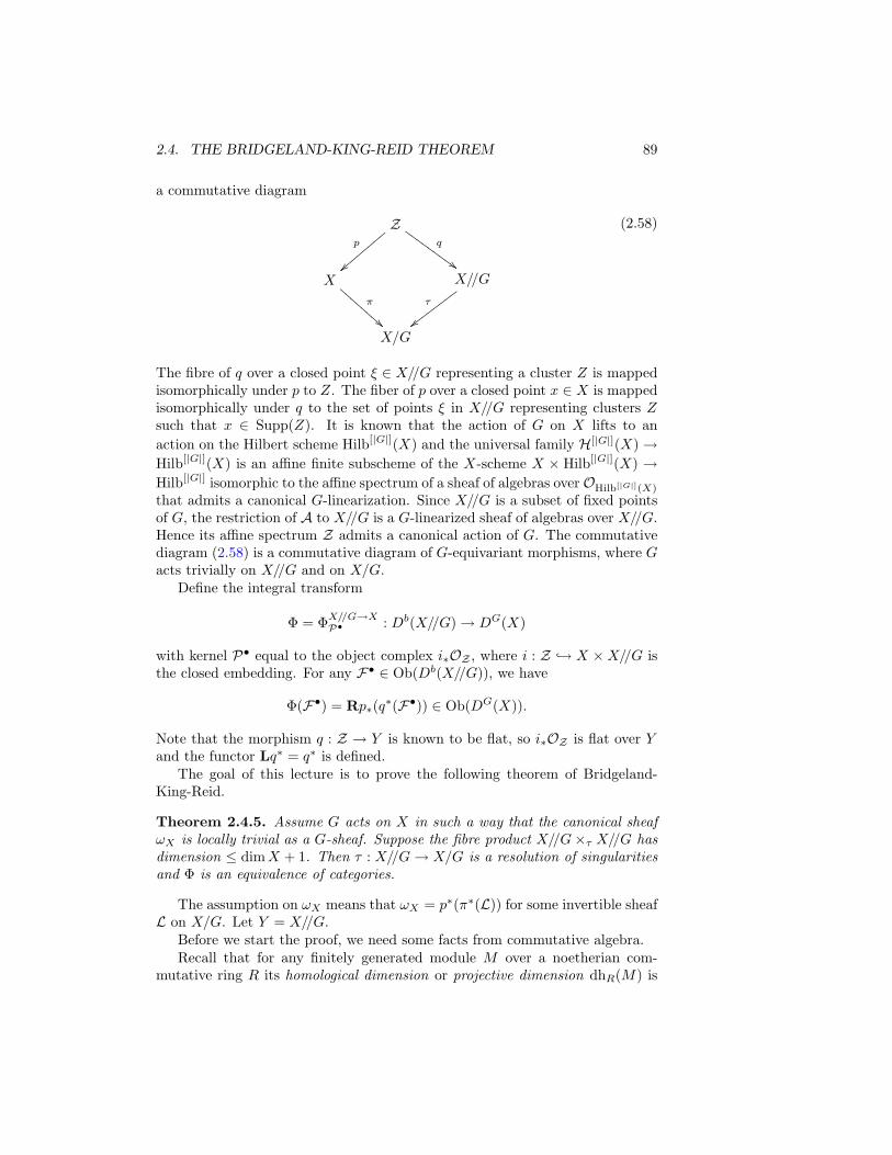
2.4. THE BRIDGELAND-KING-REID THEOREM 89
a commutative diagram
Zp
zzzzzzzzq
##HHHHHHHHH
X
π
!!CCC
CCCC
C X//G
τ
wwwwwwww
X/G
(2.58)
The fibre of q over a closed point ξ ∈ X//G representing a cluster Z is mappedisomorphically under p to Z. The fiber of p over a closed point x ∈ X is mappedisomorphically under q to the set of points ξ in X//G representing clusters Zsuch that x ∈ Supp(Z). It is known that the action of G on X lifts to anaction on the Hilbert scheme Hilb[|G|](X) and the universal family H[|G|](X)→Hilb[|G|](X) is an affine finite subscheme of the X-scheme X × Hilb[|G|](X) →Hilb[|G|] isomorphic to the affine spectrum of a sheaf of algebras overOHilb[|G|](X)
that admits a canonical G-linearization. Since X//G is a subset of fixed pointsof G, the restriction of A to X//G is a G-linearized sheaf of algebras over X//G.Hence its affine spectrum Z admits a canonical action of G. The commutativediagram (2.58) is a commutative diagram of G-equivariant morphisms, where Gacts trivially on X//G and on X/G.
Define the integral transform
Φ = ΦX//G→XP• : Db(X//G)→ DG(X)
with kernel P• equal to the object complex i∗OZ , where i : Z → X ×X//G isthe closed embedding. For any F• ∈ Ob(Db(X//G)), we have
Φ(F•) = Rp∗(q∗(F•)) ∈ Ob(DG(X)).
Note that the morphism q : Z → Y is known to be flat, so i∗OZ is flat over Yand the functor Lq∗ = q∗ is defined.
The goal of this lecture is to prove the following theorem of Bridgeland-King-Reid.
Theorem 2.4.5. Assume G acts on X in such a way that the canonical sheafωX is locally trivial as a G-sheaf. Suppose the fibre product X//G×τ X//G hasdimension ≤ dimX + 1. Then τ : X//G→ X/G is a resolution of singularitiesand Φ is an equivalence of categories.
The assumption on ωX means that ωX = p∗(π∗(L)) for some invertible sheafL on X/G. Let Y = X//G.
Before we start the proof, we need some facts from commutative algebra.Recall that for any finitely generated module M over a noetherian com-
mutative ring R its homological dimension or projective dimension dhR(M) is
90 LECTURE 2. DERIVED MCKAY CORRESPONDENCE
defined to be the largest n such that ExtnR(M,N) 6= 0 for some finitely gener-ated R-module N . We have dhR(M) ≤ n if and only if M admits a projectiveresolution
0→Mn → . . .→M1 →M0.
Recall that the depth depthR(I) of an ideal I is defined as the maximal lengthof a regular sequence in R. If R is a Cohen-Macaulay ring, then depthRI =dimR/I ([Eisenbud], Chap. 18). We have (loc. cit., Corollary 18.5)
dhR(M) ≥ depthR(Ann(M),
where Ann(M) is the annihilator ideal of M . If (R,m) is a regular local ring,then the equality always takes place. In particular, we have dh(R/m) = dimR.The next very deep result, known as the Intersection Theorem (see P. Roberts,Intersection theorems, in Commutative algebra (Berkeley, 1987), MSRI Publ.15, Springer, 1989) shows that the converse is true.
Theorem 2.4.6. Let (R,m) be a local algebra of dimension d. Suppose that
0→M−s →M−s+1 → . . .→M0 → 0
is a complex of finitely generated free R-modules with homology module Hi(M•) =H−i(M•) of finite length over R. Then s ≥ d and s = d and H0(M•) ∼= R/mimplies that M• is a free resolution of R/m and R is regular.
Now we have to extend all of this to complexes of coherent sheaves. Wedefine the support Supp(F•) of a bounded complex F• of coherent sheaves on aschemeX as the union of supports of the homology sheavesHi(F•) := H−i(F•).The homological dimension dh(F•) of a non-zero F• is the smallest i such thatF• is quasi-isomorphic to a complex of locally free sheaves of length i+ 1. Forexample, dh(F•) = 0 if and only if F• is quasi-isomorphic to E [r], where E isa locally free sheaf. The spectral sequence (2.17) gives, for any closed pointx ∈ X, the spectral sequence
Ep,q2 = ExtpX(Hq(F•),Ox) =⇒ Homp+qD(X)(F
•,Ox).
It shows that
x ∈ Supp(F•)⇔ HomiD(X)(F•,Ox) 6= 0 for some i ∈ Z.
Consider the inclusion map i : x → X and apply the adjunction of the functorsLi∗ and Ri∗ to obtain
RHomx(F•L⊗Ox) ∼= RHomi
D(X)(F•,Li∗Ox)
(here we consider Ox as a sky-scraper sheaf on X and also as a sheaf on x).Taking cohomology, and using spectral sequence (2.17), we get
Hi(F•L⊗Ox)∨ ∼= Homi
D(X)(F•,Ox). (2.59)
2.4. THE BRIDGELAND-KING-REID THEOREM 91
It is clear that if dh(F•) ≤ s, then Hi(F•L⊗ Ox) = 0 for all x ∈ X unless
j ≤ i ≤ s+ j for some j. One can show that the converse is also true. We skipthe proof (see T. Bridgeland, A. Maciocia, JAG, 11 (2002)). Let η be a genericpoint of an irreducible component Si of Supp(F•). Take a complex of locallyfree sheaves E• of length ≤ s quasi-isomorphic to F•. Restricting E• to OX,η,we obtain a non-zero complex of free OX,η-modules of length m ≤ s + 1 withfinite cohomology modules. Applying the Intersection Theorem, we obtain thats+ 1 ≥ dimOX,η = codimSi. This implies the following.
Corollary 2.4.7.codim(Supp(F•)) ≤ dh F•.
Next we need a general result (due to Bridgeland) on equivalence of derivedcategories.
Definition 2.4.2. A subset of objects Ω of a derived category is called a span-ning set if Homi(A,X) = 0 for all i ∈ Z and all A ∈ Ω implies that X ∼= 0 andHomi(X,A) = 0 for all i ∈ Z and all A ∈ Ω implies that X ∼= 0.
Lemma 2.4.8. Let F : D → D′ be a functor of derived categories with a rightadjoint H and a left adjoint G. Assume that for a spanning set Ω in D andany A,B ∈ Ω, we have Homi
D(A,B) = HomiD′(F (A), F (B)), i ∈ Z. Then F is
a fully faithful functor.
Proof. By adjunction, we have the commutative diagram
HomiD(A,B) //
δ
HomiD(A,H F (B))
β
Homi
D(G F (A), B) // HomiD′(F (A), F (B)),
(2.60)
where the bottom and the right arrows are the adjunction isomorphisms, andthe left and the top arrows are defined by applying Homi to the adjunctionmorphism of functors idD → H F and G F → idD. If A,B ∈ Ω, thediagonal map Homi
D(A,B) → HomD′(F (A), F (B)) is a bijection, so all mapsin the diagram are bijective.
For any A ∈ Ω, consider a distinguished triangle G F (A) δ→ A → C →G F (A)[1]. Applying the functor Hom(A, ?), we get the exact sequence
Hom−1(A,B)→ Hom−1(G F (A), B)→ Hom(C,B)→ Hom(A,B)
→ Hom(G F (A), B)→ . . . .
By the above, we infer that Homi(C,B) = 0 for all B ∈ Ω. Hence C ∼=0 and G F (A) → A is an isomorphism. Now take any B ∈ Ob(D) andconsider a distinguished triangle B → H F (B) → C → B[1]. Since G F (A) → A is an isomorphism, the commutative diagram (2.60) implies thatthe homomorphism Homi
D(A,B) → HomiD(A,H F (B)) is an isomorphism.
92 LECTURE 2. DERIVED MCKAY CORRESPONDENCE
The long exact sequence shows that HomiD(A,C) = 0 for all A ∈ Ω, hence
C ∼= 0, and B → H F (B) is an isomorphism for any B. Thus HomD(A,B) ∼=HomD(A,H F (B)) = HomD′(F (A), F (B)) implies that F is fully faithful.
Definition 2.4.3. A triangulated category D is called decomposable if thereexists two full subcategories D1 and D2, each containing objects non-isomorphicto the zero object, such that
(i) any object X in D is isomorphic to the bi-product of an object A1 fromD1 and an object A2 from D2;
(ii) HomiD(A1, A2) = Homi
D(A2, A1) = 0 for all i ∈ Z and allA1 ∈ Ob(D1), A2 ∈Ob(D2).
Recall that the biproduct of objects A,B in an additive category is an objectwhich is the direct sum and the direct product of A and B (i.e. corepresentsthe product of hA × hB and represents the product hA × hB).
Note that, if Ai ∈ Ob(Di) in the definition, then Ai[r] ∈ Di for any r ∈ Z.In fact, obviously Homi
D(A2, Ai[r]) = Homi+r(A2, A1) = 0 for all i ∈ Z. If A1[r]is the bi-product of A ∈ Ob(D1) and B ∈ Ob(D2) with B 6∼= 0, then there is anon-zero morphism B → A1[r]. Thus B must be a zero-object, and hence A1[r]is an object of D1.
One can restate the condition about the biproduct by saying that for anyobject X in D there is a distinguished triangle A1 → X → A2 → A1[1], whereAi ∈ Ob(Di). Since A1[1] ∈ Ob(D1), the morphism A2 → A1[1] is the zeromorphism. One can prove that this implies that the triangle splits, i.e. there isa section A2 → B. Applying the functors Hom(X, ?) and Hom(?, X), we obtainthat B is the bi-product of A1 and A2.
Example 2.4.9. Let X be a connected scheme. Let us prove that Db(X) isindecomposable. Suppose it is decomposable with subcategories D1 and D2
satisfying the definition. We may assume that OX is an object of D1. Since Xis connected, Hom(OX ,Ox) 6= 0, for all x ∈ X, hence OX belongs to D1. Forany A• ∈ Ob(D2), x ∈ X and any i ∈ Z, we must have Hom(A•,Ox[i]) = 0.Consider the spectral sequence
Ep,q2 = Homp(H−q(A•),Ox) =⇒ Homp+q(A•,Ox)
and choose q minimal with H−q(A•) 6= 0. For any point x in the support ofH−q(A•) we have Hom(H−q(A•),Ox) 6= 0. Then the term E0,q0
2 survives in thelimit and we get Homq0(A•,Ox) 6= 0. This contradiction shows that all objectsin D2 are isomorphic to zero.
Example 2.4.10. Let X be a quasi-projective irreducible variety and G be aconstant finite group of order prime to the characteristic acting faithfully onX. Then DG(X) is irreducible. In fact, suppose we have two full subcategoriesD1 and D2 as in the definition. If F is an irreducible G-sheaf , i.e it is notisomorphic to the direct sum of two non-zero sheaves, then F belongs to one
2.4. THE BRIDGELAND-KING-REID THEOREM 93
of the categories, say D1. Take F to be OZ , where Z is a free orbit. It isobviously an irreducible sheaf. Consider the surjection OX → OZ . Recall thatH0(OZ) ∼= k[G] as linear representations. Let Vρ be an irreducible k[G]-modulecorresponding to some irreducible representation of G. We consider it as a freesheaf of rank dim ρ. Then we have a nontrivial G-morphism Vρ → OZ . Thussheaves isomorphic to Vρ, they are obviously irreducible, belong to the samecategory D1. Any G-sheaf supported at a point has a section, so we can mapone of Vρ non-trivially to such a sheaf. Thus all such sheaves belong to D1.Finally, for any G-sheaf F with x ∈ Supp(F), we have a canonical non-trivialG-homomorphism F → i∗i
∗F , where i : x → X. Thus all non-zero G-sheavesare isomorphic to sheaves in D1. We know that all their shifts F [i] belong toD1. Suppose we have an object (F•, d) in D which is not isomorphic to the zeroobject. Then the complex ker(ds)[−s] is mapped to F • and the correspondingmap on the cohomology is not-trivial. Thus this is not the zero morphism inthe derived category, hence F• is an object of D1. Thus D2 consists of onlyzero objects. This proves the assertion.
Corollary 2.4.11. Under assumption of Lemma 2.4.8 assume that not everyobject in D is isomorphic to the zero object and D′ is indecomposable (i.e. notdecomposable). Suppose H(B) = 0 implies G(B) = 0. Then F is an equivalenceof categories.
Proof. Consider a full subcategoryD′1 ofD′ that consists of objects A1 such thatF H(A1) ∼= A1 and a full subcategory D′2 of objects A2 such that H(A2) ∼= 0.For any A1, A2 as above, we have
HomiD′(A1, A2) ∼= Homi
D′(F H(A1), A2) ∼= HomiD(H(A1),H(A2)) = 0,
HomiD′(A2, A1) = Homi
D′(A2, F H(A1)) ∼= HomiD(G(A2),H(A1)) = 0,
where we used the assumption H(A2) = 0 implies G(A2) = 0. For any objectB in D′, consider a distinguished triangle
F H(B)→ B → C → F H(B)[1] (2.61)
Since F is fully faithful and is left adjoint to H, the canonical morphism offunctors H F → idD is an isomorphism. Applying H, we get (H F ) H(B) ∼= H(B) → H(B) is an isomorphism. This implies H(C) ∼= 0 and henceC ∈ Ob(D′2). Also F H(F H(B)) ∼= F (H F ) H(B) ∼= F H(B). Thisimplies that F H(B) ∈ Ob(D′1). Since the morphism C → F H(B)[1] iszero, there is a left inverse of B → C (see the proof of Corollary 1.3.8). Thisimplies that B is isomorphic to the bi-product of F H(B) and C. Since B wasan arbitrary object, this contradicts the assumption that D′ is indecomposable.Thus D′2 or D′1 must consist of zero objects. If D′1 consists of zero objects, thenany object is isomorphic to an object from D′2, hence H sends all objects to thezero objects. However, we know that H F ∼= idD, and we assumed that Dcontains non-zero objects. Thus D′2 consists of zero objects. Consider again thetriangle (2.61). Since H(C) = 0 implies C ∼= 0, we get that F H(B) → B isalways an isomorphism. Thus F is an equivalence of categories.
94 LECTURE 2. DERIVED MCKAY CORRESPONDENCE
We will also need the following known result from the deformation theory.We skip its proof.
Lemma 2.4.12. Let Q be a sheaf on X × Y flat over Y . For any closed pointy ∈ Y , let Q(y) = pr∗Y (Oy)⊗Q. Then the homomorphism
pr∗Y : Ext1Y (Oy,Oy)→ Ext1X(Qy,Qy)
is the Kodaira-Spencer map TyY → Ext1X(Qy,Qy) at the point y to the schemeQuot(Y ) parameterizing sheaves on Y with Hilbert polynomial equal to the Hilbertpolynomial of Qy.
Now we are ready to start proving Theorem 2.4.5. We first start with thecase when X is projective. Let Y = X//G and n = dimX = dimY .
Step 1 : Since Z → Y is flat and X is smooth, the sheaf OZ on X×Y is of finitehomological dimension (i.e. has a finite locally free resolution). This implies thatthe complex O∨Z is of finite homological dimension. This allows one to define theintegral transform Ψ : DG(X) → Db(Y ) with kernel P• = O∨Z ⊗ pr∗XωX [n] ∈Db(X×Y ). It is equal to the composition of three functors G1 G2 G3, whereG1 = RprGY ∗, G2 = O∨Z⊗?, and G3 = pr∗X . The functor Φ is the composition ofthree functors F3 F2 F1, where F1 = pr∗Y , F2 = OZ⊗?, F3 = RprX∗. If weprove that Gi is left adjoint to Fi, then we prove that Ψ is a left adjoint to Φ.We go in all these troubles because we do not know whether Y is nonsingular.Otherwise we can apply directly Proposition 2.4.3. Clearly, G3 is left adjoint toF3. Applying (2.23) , we obtain that G2 is a left adjoint of F2. The morphismf = prY : X×Y → Y is smooth and the relative canonical sheaf ωf is isomorphicto pr∗XωX . Applying the relative duality theorem from Example 2.1.8 and takingthe invariants, we obtain that G1 is left adjoint to F1.
If Φ is a Fourier-Mukai transform, then Ψ must be its quasi-inverse functor.So we have to prove that Ψ is a quasi-inverse of Φ. Let Ψ Φ = ΦY→YQ• , whereQ• ∈ Ob(Db(Y × Y )).
Step 2 : Let y be a closed point of Y and iy : y×Y = Y → Y ×Y be the closedembedding of the fibre pr−1
1 (y) identified with Y . The restriction of the secondprojection p2 : Y × Y → Y to pr−1
1 (y) is an isomorphism, hence
ΦQ•(Oy) = (pr2)∗(Q•L⊗ pr∗1(Oy)) ∼= (pr2)∗(Li
∗y(Q•)) ∼= Li∗y(Q).
We also have O(y1,y2)∼= iy1,∗Oy2 . Using the adjunction of the functors Li∗y and
iy,∗ and of the functors Φ,Ψ, we obtain
HomiD(Y×Y )(Q•,O(y1,y2)) = Homi
D(Y×Y )(Q•, iy1,∗Oy2) = HomiD(Y×Y )(Li
∗y1Q,Oy2)
∼= HomiD(Y )(ΨΦ(Oy1),Oy2) ∼= Homi
DG(X)(Φ(Oy1),Φ(Oy2)) ∼= ExtiX(OZy1,OZy2
)G.
Step 3 : We show that
HomDG(X)(OZy1,OZy2
) ∼=
k if, Zy1 = Zy20 otherwise.
.
2.4. THE BRIDGELAND-KING-REID THEOREM 95
We have
HomDG(X)(OZy1,OZy2
) ⊂ HomX(OX ,OZy2)G = HomG(k, k[G]) ∼= k.
If y1 6= y2, there are no maps, if y1 = y2 there are only constant maps. Byassumption that ωX ∼= OX as a G-sheaf, we obtain OZy
⊗ ωX ∼= OZy(because
π maps Zy to a closed point on X/G). Applying Serre’s functor, we have
HomnDG(X)(OZy1
,OZy2) ∼= HomDG(X)(OZy2
,OZy1)∨.
Since any coherent sheafM on Y ×Y \∆Y has a composition series with quotientisomorphic to sheaves of the form O(y1,y2), we obtain that
HomiD(Y×Y )(Q•,O(y1,y2)) = 0, i ≤ 0, i ≥ n,
for all (y1, y2) ∈ Y ×Y \∆Y . Hence Q• restricted to Y ×Y \∆Y has homologicaldimension ≤ n− 2.
Step 4 : Since HomiD(Y×Y )(Q,O(y1,y2)) ∼= ExtiX(OZy1
,OZy2) = 0 for all i ∈ Z
when Zy1 is disjoint from Zy2 (i.e. when τ(y1) 6= τ(y2)), we obtain that thesupport of Q• is contained in Y ×X/G Y . By assumption, this fibre product isof codimension ≥ n − 1 in Y × Y . Thus codim(Supp(Q•)) ≥ n − 1. Since thehomological dimension of Q• restricted to Y ×Y \∆Y is less or equal than n−2,applying Corollary 2.4.7, we obtain that Q• is supported on the diagonal.
Step 5 : Let E• = ΨΦ(Oy). It follows from Steps 1 and 3 that ExtiD(Y )(E•,Oy′) =0 unless y′ = y. This implies that E• is supported at the point y. Thusdh(E•) ≥ n. On the other hand, (2.59) and Step 3 imply that dh(E•) ≤ n. Sup-pose we prove that H0(E•) ∼= Oy. Then the Intersection Theorem will implythat Y is nonsingular at y and E• ∼= Oy.
Step 6 : Let us prove that H0(E•) ∼= Oy. We have a canonical map of complexesE• = Ψ(Φ(OY )) → Oy. Let C• → E• → Oy → C•[1] be the correspondingdistinguished triangle in D(Y ) and let
. . .HomD(Y )(Oy,Oy)→ HomD(Y )(E•,Oy) = HomDG(X)(Φ(Oy),Φ(Oy))
→ HomD(Y )(C•,Oy)→ Ext1D(Y )(Oy,Oy))→ Ext1DG(X)(Φ(Oy),Φ(Oy))→ . . .
be the corresponding long exact sequence. By Lemma 2.4.12, the last map is theKodaira-Spencer map to the tangent space of the Hilbert scheme at the pointrepresented by the cluster Zy. Since the Hilbert scheme is a fine moduli spacethis map is injective. Since the first two terms in the sequence are isomorphicto k and the map is not trivial, this implies that HomD(Y )(C
•,Oy) = 0. Thespectral sequence (2.17) implies that H0(C•) = 0, hence H0(E•) ∼= Oy.
Step 7 : We have proved that E• ∼= Oy. By adjunction,
HomiD(Y )(Oy1 ,Oy2) = Homi
D(Y )(ΨΦ(Oy1),Oy2) ∼= HomiD(Y )(Φ(Oy1),Φ(Oy2)).
96 LECTURE 2. DERIVED MCKAY CORRESPONDENCE
Step 8 : We prove that the sheaves Oy form a spanning set in Db(Y ). We usethe spectral sequence (2.17)
Ep,q2 = Extp(H−q(F•),Oy) =⇒ Extn(F•,Oy).
Since its limit is zero for al y ∈ Y , taking p = 0, we get H−q(F•) = 0 for all q,hence F• is quasi-isomorphic to 0. Applying the Serre functor, we get the otherproperty too.
Step 9 : By Step 7 and Lemma 2.4.8, Φ is fully faithful. By Example 2.4.10,DG(X) is an indecomposable category. By Lemma 2.4.2, Φ admits a left adjointfunctor G = Ψ. Composing it with the Serre functor we get the right adjointH = S G S−1. Obviously H(F•) ∼= 0 implies G(F•) ∼= 0. Thus we can applyCorollary 2.4.11 and obtain that Φ is an equivalence of categories.
This concludes the proof in the case when X is projective.It remains to consider the quasi-projective case. Since we used several times
the Serre duality, the proof does not immediately extends to non-projective case.It follows from the proof that we have an equivalence of categories
Φc : Dc(Y )→ DGc (X), (2.62)
where the subscript indicates that we considering the derived category of com-plexes whose cohomology sheaves have compact support. Here we use somesmooth compactification of X to be able to apply the Serre functor to objectsin Db
c(X) as well as the adjunction isomorphisms. Consider the functor
Υ = RprGY ∗(ωZ/XL⊗ pr∗X(?))
It is a right adjoint of the functor Φ (the proof is similar to the proof that G1 isleft adjoint to F1 in Step 1). Since Φc is an equivalence of categories ΥΦ(Oy) ∼=Oy for any closed point y ∈ Y . This immediately implies that the complex Q•defining the kernel of the composition of the corresponding integral transformsis isomorphic to i∗(L), where L is an invertible sheaf on Y and i : Y → Y × Yis the diagonal morphism. Let s : OY → L = Υ Φ(OY ) be a map of sheavescorresponding to the adjunction morphism of functors δ : idY → Ψ Φ. Forany surjection φ : OY → Oy the map δ(φ) : Oy = OY ⊗ Oy → L ⊗ Oy isan isomorphism (because of equivalence (2.62)). This easily implies that thesection s is an isomorphism.
Since Υ : DG(X) → Db(Y ) is a right adjoint functor of Φ, we obtain thatΦ extends to a fully faithful functor Φ : Db(Y )→ DG(X). By the argument inthe proof of Lemma, it suffices to prove that Υ(F•) ∼= 0 implies that F• ∼= 0.By adjunction, Homi
DG(X)(Φ(G•),F•) = 0 for all i and all G• ∈ Db(Y ). Sinceany object in DG
c (X) is isomorphic to an object of the form Φ(G•), and objectsof the form OG·x is a spanning set (proven by a similar argument that Oy is aspanning set in Db(Y )), we obtain the assertion.
Remark 2.4.13. One can also prove that, under the assumption of the Theorem,the morphism τ : X//G→ X/G is crepant, i.e. τ∗(ωX/G) ∼= ωX//G.
2.4. THE BRIDGELAND-KING-REID THEOREM 97
Also it follows from Step 6 that the tangent space of X//G at a point y isisomorphic to the tangent space of the G-Hilbert scheme G−Hilb[|G|(X) at thepoint y. Since X//G is smooth this implies that X//G is a connected componentof G−Hilb[|G|(X). One can prove that in the case when dimX ≤ 3, the schemeG−Hilb[|G|(X) is connected (see [BKR]). This was conjectured by Nakamura.
Example 2.4.14. Let X = Spec R be an affine G-variety. Let ρ : G→ GL(V )be a finite-dimensional linear representation of G over k. For any G-variety Tconsider the morphism T → Spec k as an equivariant morphism where G actstrivially on Spec k. Let VT,ρ be the pull-back of V considered as a G-sheafon Spec k. If we identify V with the fibre of the corresponding trivial vectorbundle, then the group acts on its total space by g : (t, v)→ (g · t, ρ(g−1)(v)).
Let Z ⊂ X × Y be as above, i.e. the universal family over Y = X//G withprojections p : Z → X and q : Z → Y . We have
p∗(VX,ρ) ∼= VZ,ρ ∼= q∗VY,ρ.
Let Ψ : DG(X) → Db(Y ) be the Fourier-Mukai transform given by the kernelOZ . Then
Ψ(Vρ) ∼= qG∗ (VZ,ρ).
Let ρ∨ denote the dual representation. Obviously, V∨ρ ∼= Vρ∨ . By adjunction
HomGY (VY,ρ∨ , q∗OZ) ∼= qG∗ HomZ(VZ,ρ∨ ,OZ) ∼= qG∗ VZ,ρ.
LetR := q∗OZ , Rρ := HomG
Y (VY,ρ∨ ,R).
We haveΨ(Vρ) ∼= Rρ
andR ∼=
⊕ρ∈Ir(G)
Rρ ⊗ VY,ρ
where Ir(G) is the set of isomorphism classes of irreducible finite-dimensionallinear representations of G over k. Indeed the sum is a subsheaf of E and theirranks are equal to |G| = dim k[G]. Applying q∗ we get an isomorphism of freesheaves of rank |G|. Thus the sum is isomorphic to R.
Let X = C2 and G ⊂ SL2(C). Then X/G is an affine normal surface andthe orbit of 0 ∈ C2 is its unique singular (if G is not trivial) point of typeT = An, Dn, or En (a rational double point). The resolution τ : X//G →X/G is a minimal resolution of singularities, and τ−1(0) is the union of smoothrational curves E1, . . . , En with self-intersection equal to (−2). Let Ir(G)′ =ρ1, . . . , ρm be the set of non-trivial irreducible representations of G and aij =c1(Rρi
)[Ej ]. The classical McKay correspondence asserts that m = n and thematrix C = (−aij)+2In is the Cartan matrix of the simple root system of typeT .
98 LECTURE 2. DERIVED MCKAY CORRESPONDENCE
Let KG(X) denote the Grothendieck group of the category CohG(X) of G-linearized coherent sheaves. As we explained in Lecture 5, the Fourier-Mukaitransform ΦY→XP• : DG′(Y )→ DG(X) defines an isomorphism
ΦKG,Y→XP• : KG′(Y )→ KG(X).
Applying Theorem 2.4.5, we obtain
Corollary 2.4.15. Under assumptions of Theorem 2.4.5, the Fourier-Mukaitransform defines an isomorphism of abelian groups
KG(X) ∼= K(X//G).
Example 2.4.16. Suppose X = Cn and G ⊂ SLn(C). By Proposition 2.1.2,any bounded complex of coherent G-sheaves on X is quasi-isomorphic to abounded complex of locally free G-sheaves on X. Since any locally free sheafon X is free, it is isomorphic to the sheaf VX,ρ, where ρ is a linear represen-tation of G (see Example 2.4.14). This easily implies that KG(X) ∼= Rep(G),where Rep(G) = K(Mod(C[G])). This is a free abelian group of rank c equalto the number of isomorphism classes of irreducible representations of G, or,equivalently, the number of conjugacy classes of elements of G. It follows fromExample 2.4.14 that the generators Vρ, ρ ∈ Ir(G) are mapped to the classes [Rρ]of locally free sheaves on Y = X//G.
Let Kc(X//G) be the subgroup of K(X//G) formed by sheaves with supportin τ−1(0), where 0 is the orbit of 0 ∈ Cn. We have a natural biadditive pairing
Kc(X//G)×K(X//G)→ Z, 〈[E], [F ]〉 → p∗([E ⊗ F ]), (2.63)
where we represent [E] by a locally free sheaf and p∗ : K(Y )→ K(point).Let R = C[z1, . . . , zn] be the coordinate ring of X and DerR be its module
of derivations (the dual of Ω1R). Let α =
∑zi
∂∂zi∈ DerR be the Euler tangent
field . Consider the Koszul complex
K• : 0→ R→ DerR → Λ2DerR → . . .→ ΛnDerR
where the differentials are ω → ω ∧ α. The dual complex K•∨ is equal to
K•∨ : 0→ ΩnR → Ωn−1R → . . .→ Ω1
R → R,
with differentials δs : ΩsR → Ωs−1R defined by δs(ω) = 〈ω, α〉. Explicitly,
δs(dzj1 ∧ . . . ∧ dzjs) =s∑i=1
(−1)i+1zjidzj1 ∧ . . . ∧ dzji ∧ . . . ∧ dzjs .
The reader recognizes in these formulas the usual definition of the Koszul com-plex (see [Hartshorne], p. 245) for the set (z1, . . . , zn). Note that the sheaf onPn = Proj R associated with the module Ker(δs), s ≥ 1, is isomorphic to thesheaf ΩsPn .
2.4. THE BRIDGELAND-KING-REID THEOREM 99
We know that zi is transformed under g ∈ SLn(C) to∑aizi, where (a1, . . . , an)
is the i-th row of the matrix g−1. Also ∂∂zi
is transformed to∑bi
∂∂zi
, where(b1, . . . , bn) is the i-th column of the matrix g. This shows that α is G-invariantand the Koszul complex K• is an object of DG(Mod(R)). It is a free resolutionof the object complex R/(z1, . . . , zn) = C, i.e. H−i(K•) = 0 and H0(K•) ∼= C.We have
(Der1R)∼ = (Ω1X)∨ ∼= VX,ρ0 ,
where ρ0 is the representation of G in Cn defined by the inclusion G ⊂ SLn(C).Let
K• : 0→ OX → VX,ρ0 → . . .→ Λn(VX,ρ0)
be the complex of coherent sheaves corresponding to K•. Obviously Λi(VX,ρ0) ∼=VX,Λi(ρ0). Since G ⊂ SLn(C), the representation Λn(ρ0) is trivial, hence the lastterm in the complex is isomorphic to OX as a G-sheaf. Applying the functor p∗
we get a complex on Z
p∗(K•) : OZ → VZ,ρ0 → . . .→ VZ,Λi(ρ0) → . . .→ OZ .
Since VZ,ρ = q∗(VY , ρ), applying the projection formula, we get a complex onY = X//G
S• = q∗(p∗(K•)) : R → VY,ρ0 ⊗R → . . .→ VY,Λi(ρ0) ⊗R → . . .→ R.
Note that the complex K• is exact when restricted to Cn \ 0. Thus p∗(K•) issupported on p−1(0). Since q∗ is exact, the complex S• is supported on τ−1(0).
Now we decompose S• into direct sum of complexes corresponding to anirreducible representations ρi ∈ Ir(G) = ρ1, . . . , ρc.
q∗(K•) ∼=c⊕
k=1
S•k ,
where
S•k : Rk →c⊕i=1
R⊕a(1)ki
i → . . .→c⊕i=1
R⊕a(j)ki
i → . . .→ Rk, (2.64)
and
Λj(ρ0)⊗ ρk =c⊕i=1
a(j)ki ρi, j = 1, . . . , n− 1,
is the decomposition of the tensor product of the exterior power of ρ0 with ρkinto the direct sum of irreducible representations with multiplicities a(j)
ki . Foreach j = 1, . . . , n − 1, we can define the Mckay graph Γ(G, j) with vertices vicorresponding to irreducible representations of G and a
(j)ki edges from vk to vi.
For n = 2, this is the usual McKay graph equal to the extended Dynkin diagramof type ADE.
Now we have c complexes S•k whose cohomology are supported in p−1(0).Consider the pairing (2.63).
100 LECTURE 2. DERIVED MCKAY CORRESPONDENCE
Conjecture 2.4.17.〈[Ri], [S•j ∨]〉 = δij . (2.65)
This is known two be true for n = 2 (Gonzales-Sprinberg and Verdier) andn = 3 (Ito and Nakajima).
2.5 Exercises
2.1 Prove the existence of the spectral sequence
Ep,q2 = Ext(F•,Hq(G•)) =⇒ Ext(F•,G•).
2.2 Prove the existence of the spectral sequence
Ep,q2 = T or−p(Hq(F•),G•) =⇒ T or−p−q(F•,G•).
2.3 Prove the adjunction isomorphisms in (2.24).
2.4 Prove that an abelian category has homological dimension equal to 0 if andonly if all exact sequences split in A.
2.5 Prove the following projection formula. For any proper morphism f : X →Y of projective schemes over a field k, there is an isomorphism
Rf∗(F•)L⊗ G• ∼= Rf∗(F•
L⊗ Lf∗(G•).
2.6 Let ix : x → X be the inclusion morphism of a closed point x in a schemeX. Show that, for any complex F• one has F•(x) := Li∗x(F•) 6= 0 if and onlyif x ∈ Supp(F∗) := ∪iSupp(Hi(F∗)).2.7 Let X• be an object of Db(A) and m = maxi : Hi(X•) 6= 0. Show thatthere is an epimorphism from X• → Hm(X•)[−m] in the derived category.
2.8 Let Vectk be the category of finite-dimensional vector spaces over a field k.Show that the identity functor is a Serre functor.
2.9 Let F : C→ C′ be a functor between k-linear categories endowed with Serrefunctors S : C→ C, S′ : C′ → C′.
(i) Prove that the functors F S and S′ F are isomorphic.
(ii) Assume that F admits a left adjoint functor G : C′ → C. Then SGS′−1
is a right adjoint of F .
2.10 Let f : X ′ → X, g : Y ′ → Y be proper morphisms of schemes andf × g : X ′ × Y ′ → X × Y be their Cartesian product. Show that there exists amorphism of functors Db(Y )→ Db(X)
ΦY→XE• → Rf∗ ΦY′→X′
L(f×g)∗(E•) Lg∗.
2.5. EXERCISES 101
2.11 Consider the category C with objects schemes and morphisms MorC(X,Y )equal to Ob(Db(X×Y )). Take for compositions the composition F•G• definedin (2.37). Check that it is indeed a category and that it admits products. LetfE : X → Y be a morphism in C and f∗E = ΦY→XE• , fE∗ ∗ = ΦX→YE• . Show thatthis defines a fibred and cofibred categories over C.2.12 Let Db(X)tor be the full subcategory of Db(X) formed by complexes X•
such that Hi(X•) are torsion sheaves. Suppose ΦX→XE• is a Fourier-Mukai trans-form. Does it transform Db(X)tor to itself?2.13 Suppose c1(X) = 0. Show that the Mukai pairing is symmetric if dimXis even and alternating otherwise.2.14 Let ΦX→YK• and ΦX→YL• be two Fourier-Mukai transforms. Prove thatΦX→YK•
L⊗L•
is a Fourier-Mukai transform.
2.15 Let C be a small category defined by R,X, s, t, c, e), where R = Mor(C)and X = Ob(C) (see section 1.1). The axioms of a category are equivalent tothe following properties:
c (c× idR) = c (idR × c), s ε = idX = t ε, (2.66)c (c× idR) = idR = c (idR × ε),
(R×s,t R)×pr1,pr1 (R×s,t R) ∼= R×s,t ×R×s,t R
A category G is called a groupoid if each a ∈ R is an isomorphism. In thiscase there is a map ι : R → R defined by ι(a) = a−1 satisfying the followingconditions
c (idR × ι) = e s, c (ι× idR) = ε s, (2.67)
(i) Show that any group G defines a groupoid G with Ob(G) consisting ofone element.
(ii) Show that, for any group object G in a category S, the assignment S →G(S) defines a fibred category with values in groupoids.
(iii) Show that an equivalence relation R ⊂ X×X on a setX defines a groupoidwith ε equal to the diagonal map and i equal to the switch of the factorsmap.
2.16 A pair of objects (R,X) in a category C with fibred products is called angroupoid or a pre-equivalence relation on X if there are morphisms R s→ X,R
t→X, c : R×X R→ R, e : X → R, i : R→ R satisfying (2.66) and (2.67).
(i) Show that the Yoneda functor applied to (R,X, s, t, c, e, i) defines a fibredcategory in groupoids.
(ii) Show that, for any P ∈ Ob(C), the image of (s(P ), t(P )) : hR(P ) →hX(P )× hX(P ) is an equivalence relation on the set hX(P ).
(iii) Show that a group action σ : G×X → X in a category C defines a groupoidwith R = G×X,X = X, s = σ, t = prX and R×X R ∼= G×G×X.
102 LECTURE 2. DERIVED MCKAY CORRESPONDENCE
(iv) Show that for any P ∈ Ob(C) such that hX(P ) is a singleton, the data(hR(P ), hX(P ), hs(P ), ht(P ), hι(P ), he(P ) defines a group structure onthe set hR(T ).
(iv) Let C be a topological space and (Ui)i∈I be its open covering. SetX =
∐i∈I Ui and R =
∐i,j∈I Ui∩Uj . Define two projections s, t : R→ X
by considering the maps Ui ∩ Uj → Ui ⊂ X,Ui ∩ Uj → Uj . Showthat (R,X, s, t) generate a groupoid in Top (the groupoid generated bythe cover).
2.17 For any groupoid E = (R,X, s, t, c, ε, ι) in a category S and a fibredcategory C over S define the category of descent data. Its objects are pairs(A,α), where A ∈ C(X) and α is an isomorphism α : s∗(A) → t∗(A) satisfyingthe following conditions
c∗(α) = pr∗1(α) pr∗2(α), e∗(α) = idA. (2.68)
(i) Show that in the case when (R,X) is defined by a group action, thedefinition of a descent datum (A,α) coincides with the definition of aG-linearized object.
(ii) Consider an example of a groupoid in Top from Exercise 6.2 (iv) andthe fibred category Shab of abelian sheaves over Top. Show that for anysheaf
∐i∈I Fi over X =
∐i∈I Ui equipped with a descent data (called
in this case the gluing data there exists a unique sheaf F on X (up toisomorphism) such that F|Ui ∼= Fi, i ∈ I.
2.18 Let s, t : X → Y be two morphisms in a category C. A morphism p : Y →Z is called the co-equalizer of the pair (s, t) if the compositions p s and p tare equal, and, for any p′ : Y → Z ′ with this property there exists a morphismq : Z → Y ′ such that p′ = q p.
(i) Show that the co-equalizer of s, t : X → Y always exists in the categoryof sets and in the category of presheaves of sets on any category.
(ii) Let (X,R, s, t, c, ε, ι) be a groupoid in a category C. Let X/R be the co-equilizer of the pair (s, t) (it may not exist). Show that there exists acanonical map of presheaves hX/hR → hX/R, where hX/hR is the co-equalizer of h(s), h(t) : hR → hX in the category presheaves of sets. Givean example showing that it is not necessary an isomorphism.
2.19 Let C be a k-linear category. An object A is called simple if the naturalmap k → EndC(A) is an isomorphism. Assume that a k-linear category is fibredover a category S and let G be a constant group object in S and (X,σ) ∈ SG.
(i) Show that the set of G-linearizations on an object A ∈ C(X,σ) is a torsor(=principal homogeneous space) over the group Hom(G, k∗).
2.5. EXERCISES 103
(ii) Let A ∈ C(X,σ) be a G-invariant object (i.e. there exists an isomorphismpr∗X(A) ∼= σ∗(A)). Show that one can assign to A the cohomology class[A] ∈ H2(G, k∗) such that a G-invariant object admits a G-linearizationif and only if [A] = 0.
2.20 Let X be a projective variety over a field k and x be its closed point.Suppose F is a coherent sheaf such that HomX(F ,Ox) ∼= k. Prove that F isisomorphic to the structure sheaf of a closed subscheme of X.2.21 Suppose ΦX→YK• is an equivariant Fourier-Mukai transform. Then its kernelK• is a simple object of the category DG(X × Y ) (see Exercise 6.5).2.22 Let G = Z/2Z act on X = C2 as (x, y) → (−x,−y). Check the lastassertion from Example 2.4.14.2.23 Let H be a normal subgroup of G. Suppose there is an equivariant Fourier-Mukai transform Φ : DG(X)→ Db(X//G). Show that it defines an equivariantFourier-Mukai transform DG/H(X//H)→ Db(X//G).2.24 Suppose a non-trivial finite group of acts trivially on a quasi-projectivevariety X over a field of characteristic prime to the order of G . Show that thecategory DG(X) is always decomposable.

104 LECTURE 2. DERIVED MCKAY CORRESPONDENCE
Lecture 3
Reconstruction Theorems
3.1 Bondal-Orlov Theorem
In this section we will prove that a smooth projective variety X with amplecanonical or anti-canonical sheaf can be reconstructed from the derived categoryDb(X). We denote by n the dimension of X
First we see how to reconstruct closed points of X.
Definition 3.1.1. Let D be a k-linear derived category of some abelian category.Suppose D admits a Serre functor S : D → D. An object P in D is called apoint-like object of codimension c if
(i) S(P ) ∼= P [c];
(ii) Homi(P, P ) = 0, i < 0;
(iii) Hom(P, P ) := k(P ) is a field.
Proposition 3.1.1. Suppose X has an ample canonical or anti-canonical sheaf.Then an object F• in Db(X) is a point-like object if and only if F• ∼= Ox[r],where x is a closed point of X and r ∈ Z.
Proof. Let x be a closed point of X. Then S(Ox[r]) = (Ox ⊗ ωX)[r + n] ∼=Ox[n + r], thus (i) holds. Since Homi
X(F•(r),G•(r)) ∼= HomiX(F•,G•) and
Homi(Ox,Ox) = 0, i < 0, property (ii) holds too. We have
HomX(Ox(r],Ox[r]) ∼= HomX(Ox,Ox) ∼= HomOX,x(k(x), k(x)) ∼= k(x).
This checks (iii).Suppose P• is a point-like object in Db(X). Since Hi(S(P•)) = Hi(P• ⊗
ωX [n]) ∼= Hi+n(P•⊗ωX), condition (i) implies thatHi+n(P•⊗ωX) ∼= Hi+s(P•).Since the cohomology of P• and P ⊗ ωX both vanish or not vanish, tak-ing the largest possible j such that Hj(P•) 6= 0 and obtain that s = n andHi(P•) ∼= Hi(P• ⊗ ω) ∼= Hi(P•) ⊗ ωX for all i. Let us show that the coho-mology sheaves are supported in codimension n = dimX. Let F be a coherent
105
106 LECTURE 3. RECONSTRUCTION THEOREMS
sheaf on X such that F ⊗ ωX ∼= F . Tensoring with ω we get an isomorphismF ⊗ωX ∼= F ⊗ω⊗2
X . Continuing in this way we obtain that F ∼= F ⊗ω⊗sX , whereω⊗sX is very ample if ωX was ample. If ω−1
X were ample, we use a similar argumentby showing that F ∼= F ⊗ ω⊗−sX , where L = ω⊗−sX is very ample. Use ω⊗±sX tofind a closed embedding i : X → PN . Since i∗(F⊗L) ∼= i∗(OPN (1)) ∼= i∗(F)(1),we may assume that X ∼= PN ∼= Projk[T0, . . . , TN ] and F = M∼ for somegraded module over k[T0, . . . , TN ]. Let PM (t) be the Hilbert polynomial of M .Recall that PM (n) = dimkMn, n 0. Its degree is equal to the dimension ofthe support of F ([Hartshorne], Chap. I, Theorem 7.5). Since F ∼= F(1), wehave PM (n+ 1) = PM (n) for n large. This is possible only if the degree of thepolynomial is equal to zero. Thus dim Supp(F) = 0.
Applying this to our situation we obtain that Supp(P•) is a 0-dimensionalclosed subset Z. By property (iii), Z must be a single point. This follows fromthe following fact whose proof we leave to the reader: if Supp(F•) = Z1
∐Z2
then F• ∼= F•1 ⊕F•1 with Supp(F•1 ) = Z1 and Supp(F•2 ) = Z2.Now we combine the spectral sequences (2.12) and (2.17) to obtain a spectral
sequence
Ep,q2 =⊕k−j=q
Extp(Hj(P•),Hk(P•)) =⇒ Homp+q(P•,P•).
For any two sheaves F1 and F2 supported at a closed point x there exists anonzero homomorphism of sheaves F1 → F2. This follows from the fact that forany two modules M1,M2 over a local ring R supported at the maximal ideal mthere is a non-trivial homomorphism M1 →M2 (consider the filtrations on M1
and M2 with quotients isomorphic to R/m, then get a surjective homomorphismM1 → R/m and an injective homomorphism R/m→M2). Take q minimal suchthat E0,q
2 6= 0. By interchanging i and j, we may assume that q ≤ 0. Thenthe term E0,q
2 survives in the limit, hence Homq(P•,P•) 6= 0. By property (ii),we obtain q = 0. By property (iii), Hom(P•,P•) is a field. This implies thatthere is only one j with Hj(P•) 6= 0. Also End(Hj(P•)) must be a field, henceHj(P•) ∼= Ox, and we are done.
Example 3.1.2. The condition that ω±1X is ample is essential. Assume X is a
smooth projective variety with ωX ∼= OX . Take any closed reduced connectedsubvariety i : Y → X. Then the structure sheaf i∗OY is a point-like objectof codimension dimX. In fact, properties (i) and (ii) are obvious. We haveHomX(i∗OY , i∗OY ) = HomY (i∗i∗OX ,OY ) = HomY (OY ,OY ) is a field.
Another example is the following. Suppose we are in the situation of Theo-rem 2.4.5. It follows from the proof of this theorem that, for any closed pointy ∈ X//G, we have Φ(Oy) = OZy
, where Zy is a cluster on X correspondingto y. Since an equivalence of categories sends point-like objects to point-likeobjects, all objects OZ [s], where Z is a cluster, are point-like objects.
Definition 3.1.2. An object L of a k-linear triangulated category D is calledinvertible if for any point-like objects P in D there exists an integer s such that
3.1. BONDAL-ORLOV THEOREM 107
(i) Homs(L,P ) ∼= k(P );
(ii) Homi(L,P ) = 0, i 6= s.
Proposition 3.1.3. Let X be a smooth irreducible variety over k. Assumethat all point-like objects in Db(X) are isomorphic to complexes Ox[s] for somex ∈ X and s ∈ Z (e.g. if ω±1
X is ample). Then an object L• in Db(X) isinvertible if and only if L• ∼= L[t] for some invertible sheaf L and t ∈ Z.
Proof. Obviously L[t] is an invertible object in Db(X). Let L• be an invertibleobject from Db(X). Let P = Ox[s] be a point-like object. We have a spectralsequence
Ep,q2 = Hom(H−q(L•),Ox[p]) =⇒ Homp+q(L•,Ox).
Let Hq0 = Hq0(L•) be the nonzero cohomology sheaf with maximal possibleq. The terms E0,q0
2 and E1,q02 do not change in the limit (nothing goes in and
nothing goes out). Since Homi(L•,Ox) is allowed to be non-zero only for onei, and E0,q0
2 is not zero, we obtain that Hom(Hq0 ,Ox) = Homq0(L•,Ox) is afield and Ext1(Hq0 ,Ox) = 0. The second condition gives dh(Hq0) = 0, i.e.Hq0 is locally free ([Bourbaki, Commutative Algebra], Chap. 10, Prop. 4).The first condition gives that Hq0 is of rank 1. Since Hq0 is locally free, allEp,q02 = Extp(Hq0 ,Ox) = 0, p 6= 0, hence E0,q0−1
2 = Hom(Hq0−1,Ox) survivesin the limit and Homq0−1(L•,Ox) 6= 0. Since Homi(L•,Ox) is not zero only forone i, we get that Hq0−1(L•) = 0. Repeating the argument, we show that allcohomology sheaves vanish except Hq0 . Since the latter is an invertible sheaf,we are done.
Now we are ready to state and prove the Bondal-Orlov Theorem.
Theorem 3.1.4. Let X be a smooth irreducible projective variety with amplecanonical or anti-canonical sheaf. If Db(X) is equivalent to Db(Y ) for somesmooth irreducible projective variety, then X ∼= Y .
Proof. The proof will consist of several steps.Step 1 : As always we assume that the equivalence is an equivalence of de-
rived categories, i.e. it commutes with the shift functor and sends distinguishedtriangles to distinguished triangles. Let F : Db(X)→ Db(X) be an equivalenceof categories. Let G be its quasi-inverse functor. If S is a Serre functor inDb(X), then S′ = F S G is a Serre functor in Db(Y ). We also have theSerre functor SY = ⊗ωY [n]. We know that two Serre functors are isomorphic.This implies that F defines a bijection on the set of point-like objects. Sincewe do not assume that ω±1
Y is ample, we do not know whether all point-likeobjects in Db(Y ) are really shifted Oy, y ∈ Y . Suppose we have a point-likeobject P • in Db(Y ) which is not isomorphic to any object of the form Oy[i].Let x0 ∈ X such that F (Ox0 [a]) ∼= P • for some a ∈ Z. We know that x0 6= xfor any point x ∈ X such that G(Oy) ∼= Ox[j] for some j. This implies thatHomi
Db(Y )(P•,Oy) ∼= HomjDb(X)
(Ox0 ,Ox) = 0. Since the sheaves Oy span
108 LECTURE 3. RECONSTRUCTION THEOREMS
Db(Y ), we obtain that P • ∼= 0. Thus all point-like objects in Db(Y ) look likeOy[i].
Step 2 :By Step 1, we can apply Proposition 3.1.3. It follows that all in-vertible objects in Db(Y ) are isomorphic to objects of the form L[i], where Lis an invertible sheaf. The functor F transforms invertible objects to invertibleobjects.
Step 3 : Applying the shift functor we may assume that F (OX) ∼= L0 forsome invertible sheaf L0 on Y . But then HomX(OX ,Ox) = HomY (L,Oy[j]) =ExtjY (L,Oy) implies that j = 0. Thus F (Ox) ∼= Oy and k(x) ∼= k(y). Thisestablishes a set-theoretical bijection f between closed points of X and Y .
Step 4 : By composing the functor F with the functor ? ⊗ L−10 , we may
assume that F (OY ) ∼= OY in Db(Y ). Since dh(Ox) = n = dh(F (Ox)) = dimYwe obtain that dimX = dimY . We have
F (ωkX) = F (SkX(OX)[−kn] ∼= SkY (F (OX)[−kn] ∼= SkY (OY )[−kn] ∼= ωkY .
Since F is fully faithful, we get
H0(X,ωiX) ∼= HomX(OX , ωiX) ∼= HomY (F (OX), F (ωiX))
∼= HomY (OY , ωiY ) ∼= H0(Y, ωiY ),
for all i.The product in the canonical algebra
A(X) =∞⊕i=0
H0(X,ωiX)
can be expressed by the composition of s1 ∈ H0(X,ωiX), s2 ∈ H0(X,ωiX),
s1 · s2 = SiX(s2)[−in] s1.
Thus we see implies that F defines an isomorphism of graded canonical ringsA(X)→ A(Y ). If ω±1
Y were ample, we are done.Step 5 : It remains to show that ω±Y is ample. We give two proofs. The first
one uses an original argument of Bondal and Orlov. For any section s of aninvertible sheaf L, its set of zeroes (s)0 can be homologically described as theset of points x ∈ X such that the composition of the homomorphisms OX
s→L → Ox is zero. Thus we have a homological definition of a set Xs = X \ (s)0.In our situation, we obtain that F sends Ox to Of(x) and for any x ∈ (s)0,
it sends the complex OXs→ L → Ox to a complex OY
F (s)→ F (L) → Of (y).Thus the bijection f sends subsets of X of the form Xs to subsets of Y of theform YF (s). Since among sets Xf there are affine open subsets defining a baseof topology of X (take L any ample invertible sheaf), we see that the sets Xs
form a base of topology and our bijection f : X → Y is a homeomorphism.Now, on Y the open sets Yt, t ∈ Γ(Y, ω±m) are the images of open affine setsXs, s ∈ Γ(Y, ω±m) forming a base of topology of X. Hence the open sets Yt
3.1. BONDAL-ORLOV THEOREM 109
form a basis of topology in Y . It is known that this implies that ω±1Y is ample
([EGA, II 4.5.2 and 4.5.5).The second proof assumes that k is algebraically closed. We may assume
that ωX is very ample. By the argument from above the linear system |KY |separates points. In fact, if all sections of ωY vanish at y1, y2, then all sections ofωX vanish at f−1(y1), f−1(y2). Let φ : Y → Proj A(Y ) be the regular map fromY to its canonical model. Since φ separates points, no curves on Y are blowndown to points. Applying Moishezon-Nakai criterion of ampleness, we obtainthat ωY is ample. We could also prove this without appealing to the latter resultby showing that the canonical linear system |KY | separates tangent directions.We leave the argument to the reader. Similarly, we consider the case when ω−1
X
is ample.
Corollary 3.1.5. Let X be a smooth projective variety with ample canonicalor anti-canonical sheaf. Then any equivalence of derived categories Db(X) →Db(X) is a composition of f∗, where f ∈ Aut(X), a twist by an invertible sheaf,and the shift functor. More precisely, there is an isomorphism of groups
Auteq(Db(X)) ∼= (Pic(X) o Aut(X))× Z.
Proof. This follows from the proof of the previous theorem. After we shiftand twist by L = F (OX) we proved that F (OX) = OX , and then defined anautomorphism of the canonical algebra A(X). This defines an automorphism ofX.
Definition 3.1.3. Two smooth projective varieties are called derived equivalentif the exists an equivalence of their derived categories of coherent sheaves.
Using Orlov’s Theorem 2.2.5, one can also prove the following.
Theorem 3.1.6. Suppose X and Y are derived equivalent algebraic varieties.Then their canonical algebras are isomorphic. In particular, their Kodaira di-mensions are equal
Proof. Let ΦX→YP• : Db(X)→ Db(Y ) be a Fourier-Mukai transform and ΦY→XQ•
be its quasi-inverse with P• Q• ∼= OY in Db(Y ). Use A• = p∗13(P•)L⊗ p∗24(Q•)
to define the Fourie-Mukai transform ΦA• : Db(X × X) → Db(Y × Y ). LetX → X ×X and Y → Y × Y denote the diagonal morphisms. For brevity ofnotation we identify any sheaf on X or on Y with its direct image under thediagonal morphism. Let R• = ΦA•(ωsX) ∈ Db(Y × Y ). Then ΦY→YR• can becomputed as the composition of functors
Db(Y )ΦQ• // Db(X)
ΦωsX // Db(X)
ΦP• // Db(Y )
We know that ΦX→XωsX
= SX [−sdimX]. Since an equivalence of functors com-mutes with the Serre functor, we obtain that ΦA• = SY [−sdimY ]. By the
110 LECTURE 3. RECONSTRUCTION THEOREMS
uniqueness statement in Orlov’s Theorem, we obtain A• ∼= ωsX . Since ΦA is anequivalence of categories, we obtain that an isomorphism
HomiX×X(ωsX , ω
tX) ∼= Homi
Y×Y (ωsY , ωtY ),
for all s, t, i ∈ Z. Since the direct image functor under the diagonal morphismis exact, we have and isomorphism of vector spaces
HomiX(ωtX , ω
sX) ∼= Homi
Y (ωtY , ωsY ).
taking s = 0 we get an isomorphism of vector spaces H0(X,ωsX) ∼= H0(Y, ωsY ).As before we also show the isomorphism of the canonical rings.
Let us see what else the derived category detects. Recall that the cohomologyof a smooth projective variety over k = C come with the Hodge decomposition
Hi(X,C) =∑ ⊕
p+q=i
Hp,q(X)
satisfying hp,q := dimHp,q = hq,p.A cocycle γ ∈ H2p(X,Z) represented by an integer combination of fun-
damental classes of closed algebraic subvarieties of codimension p is called analgebraic cycle. It is known that, for any algebraic cycle γ its cohomology class[γ] belongs to H2p(X,Z) ∩Hp,p. It follows from the definition of Chern classesthat, for any coherent sheaf F its Chern classes ci(F) are cohomology classes ofalgebraic cycles in H2i(X,Z). In particular, the Mukai vector Mu([F ]) belongsto ⊕pHp,p ∩H2p(X,Q).
Proposition 3.1.7. Let ΦX→YP• be a Fourier-Mukai transform. Then the corre-sponding Fourier-Mukai transform in cohomology ΦH,X→YP• defines an isomor-phism ⊕
p−q=iHp,q(X)→
⊕p−q=i
Hp,q(Y ), −dimX ≤ i ≤ dimX.
Proof. Let δ = Mu([P•]) ∈ H∗(X ×Y,Q). Combining the Kunneth decomposi-tion
Hs(X × Y,Q) ∼=⊕i+j=s
Hi(X,Q)⊗Hj(X × Y,Q),
with the Hodge decomposition, we obtain that
δ =∑
αp′,q′ βr,s, p′ + r = q′ + s.
Let γ = γp,q ∈ Hp,q(X). It follows from the definition of the cohomologyintegral transform that
ΦH,X→YP• (γ) =dimX∑p=0
∑p′,q′,r,s
∫X
γp,q ∧ αp′,q′)βr,s ∈
⊕r,s
Hr,s(Y ).
The integral is equal to zero unless (p, q) + (p′, q′) = (dimX,dimX). Hencep− q = q′ − r′ = r − s.
3.1. BONDAL-ORLOV THEOREM 111
Remark 3.1.8. Let
HHi(X) =⊕p−q=i
Hp,q(X), HH∗(X) =⊕i
HHi(X),
HHi(X) =⊕p+q=i
Hp(X,Λq(TX)), HH∗(X) =⊕i
HH∗i(X),
where TX = (Ω1X)∨ is the tangent sheaf of X. The graded s[ace HH∗(X)
acquires a structure of a graded k-algebra and is called the Hochshild cohomologyalgebra. The graded vector space HH∗(X) is a module over HH∗(X) and iscalled the Hochshild homology space . The previous proposition asserts that theHochshild homology is invariant with respect to the Fourier-Mukai transfrom.The same is true for the Hochshild cohomology.
We have seen already in Example 2.2.7 that the assertion of Corollary 3.1.5is not true for elliptic curves whose canonical class is trivial. We state thefollowing theorem due to Polishchuk and Orlov.
Theorem 3.1.9. Two abelian varieties A and B are derived equivalent if andonly if there exists an isomorphism f : A× A→ B × B, where the hat denotesthe dual abelian variety defined as the Picard variety of linear equivalence classesof divisors algebraically equivalent to zero.
Recall that a smooth algebraic surface X is called a K3-surface if KX = 0and the first Betti number b1(X) is equal to zero (this makes sense over anyfield). If k = C, all K3 surfaces are diffeomorphic as compact 4-manifolds. Wehave H2(X,Z) ∼= Z22 and the intersection form on H2(X,Z) defined by thecup-product has signature (3, 19). It is isomorphic over Z to the orthogonalsum of even unimodular quadartic forms E⊥2
8 ⊥ U⊥3, where E8 is given bythe negative of the Cartan matrix with Dynkin diagram of type E8 and U isa hyperbolic plane. The Neron-Severi group NS(X) is a free abelian group ofsome rank 20 ≥ ρ ≥ 1. The intersection form restricted to NS(X) has signature(1, ρ − 1). The first Chern class c1 : NS(X) → H2(X,Z) is an embedding ofquadratic lattices (i.e. free abelian groups equipped with quadratic forms). Wewill identify NS(X) with its image. Its orthogonal complement in H2(X,Z) isa free abelian group T (X) of rank 22 − ρ, called the lattice of transcendentalcycles. The Hodge decomposition
H2(X,C) = H2,0(X)⊕H1,1(X)⊕H0,2(X)
has the Hodge numbers h2,0 = h0,2 = 1, h1,1 = 20. The subspace H1,1(X) isorthogonal to H2,0(X) with respect to the intersection form on H2(X,C). SinceNS(X) is contained in H1,1(X) we see that H2,0(X) ⊂ T (X)C = TX ⊗ C.
An isometry σ : T (X)→ T (X) of quadratic lattices (defined by the intersec-tion forms) that sends H2,0(X) to H2,0(Y ) under the induced map T (X)C →T (Y )C is called a Hodge isometry . The Global Torelli Theorem due to I.Piatetski-Shapiro and I. Shafarevich asserts that any Hodge isometry that canbe extended to an isometry σ of H2(X,Z)→ H2(Y,Z) that sends the effective
112 LECTURE 3. RECONSTRUCTION THEOREMS
cone of X to the effective cone (or equivalently an ample class to an ampleclass) of Y under the induced map H2(X,R)→ H2(Y,R) is equal to g∗, whereg : Y → X is an isomorphism of surfaces. By applying some isometry ofH2(X,Z) identical on T (X) one can assume that σ sends the effective cone tothe effective cone. This implies that the surfaces X and Y are isomorphic.
The following result is due to Orlov.
Theorem 3.1.10. Let X and Y be two complex algebraic K3 surfaces. ThenDb(X) is equivalent to Db(Y ) if and only if there is a Hodge isometry H2(X,Z)→H2(Y,Z).
We will prove only the ‘only if’ part.
Proof. Again we use Orlov’s Theorem to assume that our equivalence of cate-gories is a Fourier-Mukai transform with some kernel E• ∈ Db(X×Y ). One cancheck that the Mukai vector Mu(E•) of any E• belongs toH∗(X,Z) ⊂ H2(X,Q).By Proposition 3.1.7, taking i = 0, we obtain that the Mukai transform in co-homology sends the subspace
H0,0(X)⊕H1,1(X)⊕H2,2(X) = H0(X,C)⊕H1,1(X)⊕H2(X,C).
to the similar subspace of H∗(Y,C). It also sends the intersection of this sub-space with H2(X,Z) equal to
NS(X) = H0(X,Z)⊕NS(X)⊕H4(X,Z).
to NS(Y ). Since KX = KY = 0, it follows from Proposition 2.2.12 that theFourier-Mukai defines an isometry H∗(X,Z) → H2(Y,Z). Thus it defines anisometry of the orthogonal complements
σ : T (X) = (NS(X))⊥ → T (Y ) = NS(Y ))⊥.
Applying Proposition 3.1.7 with i = 2, we see that σC(H2,0(X)) = H2,0(Y ).Thus σ is a Hodge isometry.
Definition 3.1.4. Two K3 surfaces with equivalent derived categories of co-herent sheaves are called Fourier-Mukai partners.
Proposition 3.1.11. A K3 surface has only finitely many non-isomorphicFourier-Mukai partners.
Proof. Let Yi, i ∈ I be the set of representatives of isomorphism classes ofFourier-Mukai partners of a K3 surface X. Assume this set if infinite. It fol-lows from the proof of Theorem 3.1.10 that an equivalence of derived categoriesDb(Yi) → Db(X) defines an isomorphism of lattices NS(Yi) → NS(X) and aHodge isometry σ : T (Yi)→ T (X). Since the lattice H0(X,Z)+H4(X,Z) is iso-morphic to a hyperbolic plane, a theorem from the theory of integral quadraticforms implies that the lattices NS(X) and NS(Y ) are in the same genus (i.e.isomorphic over any ring of p-adic numbers Zp). It is known that there are only
3.2. SPHERICAL OBJECTS 113
finitely many non-isomorphic forms in the same genus. Thus there are infinitelymany Fourier-Mukai partners Yi with the Neron-Severi lattices NS(Yi) isomor-phic to NS(X). Let H = H2(X,Z),M = NS(X), T = T (X)⊥ considered asabstract lattices. The lattice T is equipped with a Hodge structure, i.e a linein H ⊗ C. For any non-degenerate lattice N let N∨ = Hom(N,Z) be the duallattice. It is equipped with the symmetric bilinear form induced from the latticeN ⊗Q ∼= Hom(N,Q). Since the lattices M and T are non-degenerate, the natu-ral map (M ⊥ T )→ (M ⊥ T )∨, v 7→ (v, ?) has finite cokernel. Its order is equalto the absolute value of the discriminant of the quadratic form on M ⊥ T . Wehave an inclusion of lattices N = M ⊥ T ⊂ H ⊂ N∨ = (M ⊥ T )∨. The numberof intermediate lattices between N and N∨ is finite and is equal to the numberof subgroups of coker(M ⊥ T ) → (M ⊥ T )∨). Thus we can find an infiniteset of Yj , j ∈ J ⊂ I, such that the isomorphism NS(Yi) ⊥ T (Yi) → M ⊥ Tlifts an isomorphism H2(Yi,Z) → H ′, where H ′ lies between M ⊥ T and(M ⊥ T )∨. Replacing X with one of the Yj , we see that there are infinitelymany Yi’s such that the Hodge isometry T (Yi) → T (X) lifts to an isometry ofH2(Yi,Z) → H2(X,Z). Applying the Global Torelli Theorem, we obtain thatall such Yi’s are isomorphic to X. This contradiction proves the assertion.
One can give an explicit formula for the number of Fourier-Mukai partnersin terms of the structure of the Neron-Severi lattice NS(X).
3.2 Spherical objects
Corollary 3.1.5 on auto-equivalences of the derived category of a variety withample canonical or anti-canonical sheaf does not extend to varieties which donot satisfy this condition. For example, in the case of a K3 surface, many newanti-equivalences arise from spherical objects.
Definition 3.2.1. An object E in a k-linear triangulated category D with aSerre functor S is called spherical if
(i) S(E) ∼= E[n], for some n ∈ Z;
(ii)
HomD(E,E[i]) =
k if, i = 0, n0 otherwise.
Example 3.2.1. Assume KX = 0 and hi(OX) = 0, 0 < i < n = dimX (i.e. Xis a Calabi-Yau manifold). Any invertible sheaf is a spherical object. Condition(i) holds obviously with n = 2. We have
Hom(L,L[i]) = Hom(OX ,OX [i]) ∼= Hi(X,OX).
This is not equal to zero only if i = 0,dimX.
114 LECTURE 3. RECONSTRUCTION THEOREMS
Also let R be a smooth rational curve on X such that the normal bundleNR/X is isomorphic to OP1(−1)⊕n−1. Let i : R → X be the closed embedding.Let us see whether i∗OR is a spherical object. We have an isomorphism
ExtiX(i∗OR, i∗OR) ∼= ΛiNR/X . (3.1)
In fact, consider the exact sequence
0→ JR → OX → i∗OR → 0
and apply HomX(?, i∗OR) to get an exact sequence
0→ HomX(i∗OR, i∗OR)→ HomX(OX , i∗OR)→ HomX(JR, i∗OR)
→ Ext1X(i∗OR, i∗OR)→ 0.
It is easy to see that HomX(JR, i∗OR) ∼= NR/X ∼= (JR/J 2R)∨. This gives an
isomorphism (3.1) for i = 0, 1. For i > 1, we consider the induced isomorphism
ΛiNR/X → ExtiX(i∗OR, i∗OR),
where the target is given by the cup-product of Ext1X(i∗OR, i∗OR)’s. Now weuse the spectral sequence
Ep,q2 = Hp(X, ExtqX(i∗OR, i∗OR)) =⇒ Extp+q(i∗OR, i∗OR)).
We haveΛqNR/X ∼=
⊕Λq(OP1(−1)⊕n−1) ∼= OP1(−q)⊕(n−1
q ).
This implies that Ep,q2 6= 0 only if p = q = 0 and p = 1, q ≥ 2. This easilyimplies that i∗OR is a spherical objects if and only if n = 3.
If n = 2, and R is a smooth rational curve, the sheaf OR is a sphericalobject. We use that R is a (−2)-curve, i.e. R ∼= P1 and R2 = −2. We havek = H0(OR,OR) ∼= H2(OR,OR) and playing with the exact sequence
0→ OX(−R)→ OX → OR → 0
gives easily Ext1(OR,OR) = 0 (use that Hom(OX(−R),OR) ∼= Hom(OX ,OR(R)) ∼=H0(R,OX(−2)) = 0).
Another example of a spherical object on a K3 surface X is a simple rigidvector bundle (see Example 2.2.14). As we remarked earlier in Lemma 2.4.12,the space Ext1(E , E) is the tangent space to the moduli space of simple bundlesat the point [E].
Definition 3.2.2. A triangulated k-linear category D is called to be of finitetype if, for any objects A and B in D,
dimk Hom•D(A,B) <∞ (3.2)
whereHom•
D(A,B) =⊕i∈Z
HomiD(A,B),
3.2. SPHERICAL OBJECTS 115
For example, D = Db(X), where X is projective, satisfies this condition.For any objects E,F ∈ Ob(D) define the objects LE(F ) and RE(F ) in D by
means of the distinguished triangles
LE(F )→ Hom•D(E,F )⊗ E ev→ F → LE(F )[1], (3.3)
Fev→ Hom•
D(F,E)∗ ⊗ E[i]→ RE(F )→ F [1]. (3.4)
Here the tensor product means the complex whose j-th component is equalto the direct sum of complexes ⊕iE[−i]⊕di , where di = dimk Homi
D(E,F ). Themorphism ev is defined by means of an isomorphism Homi
D(E,F ) ∼= HomD(E(−i), F )and sending the copy of E[−i] with index φ ∈ Homi
D(E,F ) to F by means ofφ. Similrly one defines the tensor product and the evaluation morphism in thesecond triangle.
One can show that the operations LE and RE define functor of triangulatedcategories.
Assume E is a spherical object in D. Our first observation is that
LE(E) ∼= E[−n], RE(E) ∼= E[n]. (3.5)
Indeed we have a distinguished triangle
LE(E)→ E ⊕ E[−n]→ E → LE(E)[1].
It is easy to see that it is isomorphic to the direct sum of the distinguished
triangles 0 → E → E → 0[1]→ 0 and E[−n] → E → 0 → E[1 − n]. A similar
argument applies to RE .Our second observation is that
LE(F ) ∼= F [−1], RE(F ) ∼= F ]1] (3.6)
if HomD(E,F [i]) = 0 for all i ∈ Z.Our third observation is that there are isomorphisms of functors
LE[1]∼= LE , RE[1]
∼= RE (3.7)
From now on, let D = Db(X), where X is a smooth projective n-dimensionalvariety. Let i : ∆ → X × X be the diagonal map. Consider the naturalhomomorphism
p∗E•L⊗ q∗E•∨ → O∆
defined as the composition
p∗E•L⊗ q∗E•∨ → i∗i
∗(p∗E•L⊗ q∗E•∨) = i∗(E•∨
L⊗ E•) tr−→ O∆,
where tr : E•L⊗ E•∨ → OX is the trace map. Let
p∗E•L⊗ q∗E•∨ → O∆ → E• → p∗E
L⊗ q∗E•∨[1] (3.8)
116 LECTURE 3. RECONSTRUCTION THEOREMS
be a distinguished triangle.We claim that
LE• := ΦX→XE• = Rq∗ E•L⊗ p∗
To see this explicitly, we apply the integral transform to the distinguished tri-angle (3.8) to get the distinguished triangle
Rp∗(p∗(E•)L⊗ q∗(E•∨
L⊗F•))→ Rp∗(O∆
L⊗F•) ∼= F• → LE•(F•)
[1]→
Using the projection formula, we obtain
Rp∗(p∗(E•)⊗ q∗(E•∨L⊗F•)) ∼= E• ⊗RHom(E•,F•),
where RHom•(E•,F•) is considered as a complex of free sheaves. Writing downthe tensor product explicitly, we obtain a distinguished triangle⊕
i∈ZHomi(E•,F•)⊗ E•[−i]→ F• → LE•(F•)
[1]→ (3.9)
Our first observation is that
LE•(E•) ∼= E•[1− n] (3.10)
Indeed, we have a distinguished triangle
E• ⊕ E•[−n]→ E• → LE•(E•)[1]→
We have a morphism LE•(E•) → E•[1] ⊕ E•[1 − n] → E•[1 − n]. Applying thecohomology we see that it defines a quasi-isomorphism.
Our second observation is that
LE•(F•) ∼= F• (3.11)
if Hom(E•,F•[i]) = 0 for all i ∈ Z.Our third observation is that
LE•[1] ∼= LE• (3.12)
Example 3.2.2. Assume dimX = 1. For any closed point x ∈ X the sheafOx is a spherical object (use the Serre duality). Suppose F• = F is a locallyfree sheaf of rank r. We have Homi(Ox,F) = 0, i 6= 1 and Hom1(Ox,F) ∼=Hom(F ,Ox)∨. The distinguished triangle becomes
Hom(F ,Ox)∨ ⊗Ox[−1]→ F → LOx(F)→ Hom(F ,Ox)∨ ⊗Ox
This easily implies that LOx(F) is a locally free sheaf and, passing to duals, we
get an exact sequence of sheaves
0→ LOx(F)∨ → F∨ → F∨(x)→ 0,
3.2. SPHERICAL OBJECTS 117
where for any sheaf G we denote by G(x) its fibre at x (not the stalk), i.e.Gx/mX.xGx). For any non-zero linear function α : F∨(x)→ k(x) the pre-imagein F∨ of the kernel of α is a locally free subsheaf of F∨ of rank r. The data(x, α) defines the classical elementary operation elmx,α on locally free sheaves.Assume r > 1 and consider the vector bundle V(F) associated to F , then αdefines a nonzero point in the fibre V(F)x. Passing to the projective bundlesPV(F) = Proj Sym•(F) we consider α as a point in the fibre PV(F)x. We canblow-up this point, and then blow down the proper transform of the fibre, theresult is a projective bundle isomorphic to PV(elmx,α(F)).
Note that if r = 1 and F = OX(D) for some divisor D, then TOx(F) ∼=
OX(D − x).
Assume E is a spherical object. The twist functors LE and RE is called thespherical twists.
We want to show the spherical twist is a Fourier-Mukai transform. We needthe following.
Lemma 3.2.3. Suppose ΦX→YP• is a fully faithful integral transform with kernelP•. Then it is a Fourier-Mukai transform if and only if dimX = dimY and
P• ⊗ p∗ωX ∼= P• ⊗ q∗ωY .
Proof. We have seen already that these conditions are necessary. To provethe sufficiency, we use that F = ΦX→YP• has the right adjoint functor H andthe left adjoint functor G defined by the integral transforms with kernel P• ⊗p∗ωX [dimX] and P• ⊗ q∗ωY [dimY ], respectively. It follows from Corollary2.4.11 that F is an equivalence of categories if H(B) = 0 implies G(B) = 0.Since, by assumption, G ∼= B, the assertion follows.
Theorem 3.2.4. Let E• be a spherical object in Db(X). Then
LE• := ΦX→XE•
is a Fourier-Mukai transform.
Proof. Applying the previous lemma, it suffices to show that
E• ⊗ p∗ωX ∼= E• ⊗ q∗ωX .
and that LE• is fully faithful. The first claim is rather obvious since a distin-guished triangle (3.8) defines a distinguished triangle
q∗(E•∨ ⊗ ωX)L⊗ p∗E• → O∆ ⊗ q∗ωX → E• ⊗ q∗ωX
[1]→ . . .
and the same is true if we exchange the roles of the projections p and q.We use Proposition 2.4.8, taking for the spanning set Ω the set of objects
in Db(X) that consists of E• and the set E•⊥ consisting of all objects G• suchthat HomDb(X)(E•,G•[i]) = 0 for all i ∈ Z. Let us prove that it is a spanning
118 LECTURE 3. RECONSTRUCTION THEOREMS
set. Obviously, if HomDb(X)(G•,F•[i]) = 0 for all G• ∈ Ω and all i ∈ Z, thenF• must be in E⊥. But then HomDb(X)(F•,F•) = 0 implies F• ∼= 0. Nowsuppose HomDb(X)(F•,G•[i]) = 0 for all G• in Ω and all i ∈ Z. Applying theSerre functor, we get 0 = HomDb(X)(F•, E•[i]) = HomDb(X)(F•, S(E•[i−n])) =HomDb(X)(E•[i−n],F•) for all i. This implies that F• ∈ E•⊥, and we finish asbefore.
Next we need to show that
LE• : Hom(G•1 ,G•2 [i])→ Hom(LE•(G•1 ), LE•(G•2 [i]))
is a bijection for all i ∈ Z. This is obviously true if G•1 = E• and G•2 ∈ E•⊥. Byusing observations (3.10) and (3.11), we see that this is true if G•1 = G•2 and ifG•1 ,G•2 ∈ E•⊥.
Let us see how the spherical twist LE• acts on the cohomology. Let v ∈H∗(X,Q) and [E•] be the class of E• inK0(X×X). It follows from the definitionthat [E•,•] = [O∆] − p∗([E•∨] ⊗ q∗([E•]). Its Mukai vector in H∗(X ×X,Q) isequal to [∆]− p∗(Mu(E•∨) · q∗(Mu(E•)). We know that
LHE•(v) := ΦH,X→XE•,• (v) = q∗(Mu([E•]) · p∗(v))
= v −(∫X
v ·Mu(E•∨))v = v −
(∫X
exp(c1(X)/2)v ·Mu(E•)∨)v
= v − 〈Mu(E•), v〉Mu(E•).
Applying proposition 2.2.12, we get
〈Mu(E•),Mu(E•)〉 = χ(E•, E•) = dim Hom(E•, E•) + (−1)n dim Homn(E•, E•)
=
2 if n is even0 otherwise.
When n is even, we obtain that LHE• acts as a reflection in the vector Mu(E•), i.e.it sends this vector to its opposite, and leaves invariant any vector orthogonal toMu(E•) with respect to the pairing 〈, 〉. If KX = 0, and Mu(E•) ∈ H2(X×X,Z)(e.g. if X is a K3 surface), then the pairing is a symmetric bilinear form onH∗(X,Z) and LHE• is a reflection isometry of the corresponding lattice. Recallthat a reflection with respect to a vector α in a quadratic lattice M is itsisometry defined by the formula
rα(x) = x− 2(x, α)α, α
α,
where one assumes that (v, v) divides 2(x, v) for any x ∈M (e.g. if (α, α) = ±2).Observe that L2
E• = idH∗ but L2E•(E•) = E•[1 − n], so L2
E• belongs to thekernel of the action of Auteq(Db(X)) on the cohomology.
3.2. SPHERICAL OBJECTS 119
Example 3.2.5. Let X be a complex algebraic K3-surface. It is known thatno non-identity automorphism can act trivially on the cohomology. Thus L2
E•cannot be induced by an automorphism of X. Consider the natural homo-morphism a : Aut(X) → Aut(NS(X)). Its kernel is a finite group since itpreserves the class of any ample line bundle and, its is known, that no alge-braic group of positive dimension can act on X. Let WX be the subgroup ofO(NS(X)) generated by reflections in vector [R], where R is a smooth rationalcurve on X. It is a normal subgroup of O(X) and we can compose a withthe quotient map O(NS(X)) → O(NS(X))/WX to obtain a homomorphisma′ : Aut(X) → O(NS(X))/WX . It follows from the Global Torelli Theoremthat the cokernel of this homomorphism is a finite group. Let E• = OR, whereR as above. Then LE• acts on NS(X) as the reflection with respect to the vector[R] (note that [OR] = [R] in K0(X) and R2 = −〈Mu([R], [R]〉 = −2). Thus theimage of the subgroup of Auteq(Db(X) generated by the spherical twists LOR
in O(NS(X)) coincides with WX . Thus together with Aut(X) the cohomologyspherical twists generate a finite index subgroup of O(NS(X)).
Let us see how different spherical twists compose.
Lemma 3.2.6. Let Φ : Db(X) → Db(X) be an auto-equivalence of derivedcategories. For any spherical object E• in Db(X),
Φ LE• = LΦ(E•) Φ.
Proof. We have a distinguished triangle
RHom(Φ(E•),Φ(F•))L⊗ Φ(E•)→ F• → LΦ(E•)(Φ(F•)) [1]→ (3.13)
Since Φ is an equivalence of categories, RHom(Φ(E•),Φ(F•)) ∼= RHom(E•,F•),and applying Φ to the distinguished triangle defining LE• , we get a distinguishedtriangle
RHom(E•,F•)L⊗ Φ(E•)→ F• → Φ(LE•(F•))
[1]→ (3.14)
Comparing the two triangles, we find LΦ(E•)(Φ(F•)) ∼= Φ(LE•(F•)). Thereis a subtlety here. Although we have an isomorphism for each F•, this maynot define an isomorphism of functors. Assuming that Φ is a Fourier-Mukaitransform (e.g. applying Orlov’s Theorem), one can show that, in fact, there isan isomorphism of functors (see [Huybrechts], p. 176).
We apply this lemma, by taking Φ = LF• for some spherical object F•. Weget
LF• LE• = LLF• (E•) LF• . (3.15)
This immediately implies that LE• and LF• commute if F• ∈ E•⊥ (for example,if E• = OR,F• = OR′ , where R,R′ are two disjoint smooth rational curves ona K3 surface).
Let E•1 , . . . , E•N be a collection of spherical objects satisfying
aij = ⊕p dim Homp(E•i , E•j ) ≤ 1, i 6= j. (3.16)
120 LECTURE 3. RECONSTRUCTION THEOREMS
Let LE•i = Li. Assume aij = 1. After shifting Ei, using (3.12), we may assumethat dim Hom(E•i , E•j ) = 1. We have a distinguished triangle
E•i → E•j → Li(E•j )→ E•i [1].
Applying Lj we get a distinguished triangle
Lj(E•i )→ Lj(E•j ) = E•j [1− n]→ Lj(Li(E•j ))→ Lj(E•i )[1], (3.17)
where dimX = n. Since dim Hom(E•j , E•i ) = dimHomn(E•j , E•i ), we get a distin-guished triangle
E•j [−n]→ E•i → Lj(E•i )→ E•j [1− n].
After shifting, we have the triangle
Lj(E•i )→ E•j [1− n]→ E•i [1]→ Lj(E•i )[1].
Comparing it with triangle (3.17), we get Lj(Li(E•j )) ∼= E•i [1]. Thus LLj(Li(E•j )∼=
Li. Applying (3.15) twice, we have
Lj Li Lj = Lj LLi(E•j ) Li = LLj(Li(E•j )) Lj Li = Li Lj Li.
Summing up, we obtain the relationsLi Lj = Lj Li if aij = 0,Li Lj Li = Lj Li Lj otherwise.
(3.18)
Recall the definition of the Artin-Brieskorn braid group. Let S be a sym-metric matrix of size S with integer entries sij ≥ 2 off the diagonal and sii = 0.The Artin-Brieskorn braid group B(S) is defined by generators g1, . . . , gN withdefining relations
gi · gj · gi · · · = gj · gi · gj · · · , i 6= j,
where in each side there are sij factors. The quotient of B(S) by the normalsubgroup generated by g2
1 , . . . , g2N is the Coxeter group defined by the matrix S.
The matrix S can be defined by the Coxeter-Dynkin diagram. It is a graph withvertices vi, i = 1, . . . , N, joined by sij−2 edges. Conversely such diagram definesa matrix S as above. For example, the Coxeter group with the Coxeter-Dynkindiagram
• • • •
is the symmetric group SN+1. The corresponding Artin-Brieskorn group is theclassical braid group BN+1 introduced by E. Artin. In our case, we take S =(sij), where Sij = aij+2, to obtain that the subgroup of Auteq(Db(X) generatedby L1, . . . , LN satisfies the braid relations of the Artin-Brieskorn group B(S).In particular, we have a homomorphism
ρ : B(A)→ Auteq(Db(X)).
In the case when S is of type AN , i.e. described by the Coxeter-Dynkin diagramof type AN from above, Seidel and Thomas have proved that ρ is injective ifdimX ≥ 2, i.e. the braid relations (3.18) are defining relations.
3.3. SEMI-ORTHOGONAL DECOMPOSITION 121
Example 3.2.7. Let X be a K3 surface, and R1, . . . , RN be a set of smoothrational curves such that aij = Ri ·Rj ≤ 1 for i 6= j. Using the exact sequence
0→ OX(−Ri)→ OX → ORj → 0
and applying the functor HomX(ORi, ?), we easily get
Hom2(ORj,ORi
) ∼= Ker(Ext2(ORi,OX(−Rj))→ Ext2(ORi
,OX))
= Ker(Hom(OX(−Rj)),ORi)∨ → Hom(OX ,ORj )
∨)
∼= Ker(H0(X,ORi(1))∨ → H0(X,ORi
)∨) = Ker(k2 → k) ∼= k.
All other Homi vanish. Thus the spherical objects satisfy condition (3.16) andwe have an action of the corresponding Artin-Brieskorn braid group B(A) onDb(X), where A = (aij). Note that we have a commutative diagram
B(A) //
Autoeq(Db(X))
Mu
C(A) // O(H∗(X,Z))
,
where C(A) is the Coxeter group corresponding to B(A) and O(H∗(X,Z)) isthe group of isometries of the Mukai lattice (see Example 2.2.14).
The same is true if we replace a collection of (−2)-curves Ri as above witha collection of rigid simple vector bundles Ei with dim Ext1(Ei, Ej) ≤ 1.
3.3 Semi-orthogonal decomposition
In this section we discuss how a triangulated category could be described as asort of span of its finitely many objects.
Let D be a triangulated category of finite type. We assume that it is equippedwith a Serre functor S : D→ D.
Definition 3.3.1. A full triangulated subcategory D′ of D is called right (left)admissible if the inclusion functor has a right (left) adjoint. The right (left)orthogonal D′⊥ (⊥D′) of an admissible subcategory is the full category formedby objects B such that HomD(A,B) = 0 (HomD(B,A) = 0) for all A ∈ Ob(D′).We say that D′ is admissible if it is right and left admissible.
Note that D′⊥ is a triangulated subcategory as it is easy to see by usingthat HomD(A,B[i]) = HomD(A[−i], B) = 0 and applying the functor Hom to adistinguished triangle B1 → B2 → C → B1[1] with B1, B2 ∈ Ob(D′⊥).
The meaning of being right admissible is the following. For any objectC ∈ D there exists a distinguished triangle A → C → B → A[1], where A ∈Ob(D′), B ∈ Ob(D′⊥). In fact we set A = i!(C) where i! is a right adjoint ofthe inclusion functor i : D′ → D. The identity morphism A → A defines, by
122 LECTURE 3. RECONSTRUCTION THEOREMS
the property of adjoint functors, a morphism A → C that can be extended toa distinguished triangle A→ C → B → A[1]. For any A′ ∈ Ob(D′) we have anexact sequence
Hom(A′, A) = Hom(A′, i!(C)) a→ Hom(A′, C)→ Hom(A′, B)→
Hom(A′, A[1])a[1]→ Hom(A′, C[1]),
where the morphisms a and a[1] are isomorphisms. This gives Hom(A′, B) = 0for all A′ ∈ Ob(D′), hence B ∈ D′⊥.
Conversely, suppose each C ∈ Ob(D) can be realized as the midterm ofa distinguished triangle A → C → B → A[1], where A ∈ Ob(D′) and B ∈Ob(D′⊥) for some full triangulated category D′. Then D′ is right admissible. Infact, we can can set i!(C) = A. In order this to be defined we have to show thatthe triangle is unique up to a unique isomorphism. Let A′ → C ′ → B′ → A′[1]be a distinguished triangle and f : C → C ′ be a morphism. Let us construct aunique morphism φ : B′ → B such that the following diagram is commutative
A′g //
φ
C ′ //
f
B //
A′[1]
φ[1]
A // C // B // A[1]
Since Hom∗(A′, B) = 0, applying Hom(A′, ?) to the bottom triangle, we get anisomorphism Hom(A′, A) → Hom(A′, C). The morphism φ is the pre-image off g under this isomorphism. If C ′ = C and f = idC we get the uniquenessof the isomorphism φ. For any C ∈ Ob(D) we get a distinguished triangle0 → i!C → C → B → i!(C)[1]., where B ∈ Ob(D′⊥). Applying HomD(A, ?) weget
0→ HomD(A, i!(C))→ HomD(i(A), C)→ HomD(A,B) = 0.
This shows that i! is a right adjoint to i.Our final observation is that a right (left) admissible subcategory is admis-
sible if D admits a Serre functor.For any set S of objects in D let 〈S〉 to be the smallest full triangulated
subcategory containing S among its objects. We say that S generates D ifD = 〈S〉. We say that a subcategory D′ generates D if its objects generate D.
Proposition 3.3.1. Let D′ be an admissible subcategory of D. Then D′ andD′⊥ generate D.
Proof. Any C can be included in a distinguished triangle A→ C → B → A[1],where A ∈ Ob(D′) and B ∈ Ob(D′⊥). This triangle defines the distinguishedtriangle B[−1]→ A→ C → B. By definition of a triangulated subcategory, Cmust be an object of 〈D′,D′⊥〉.
3.3. SEMI-ORTHOGONAL DECOMPOSITION 123
Remark 3.3.2. The notion of an admissible category is a generalization of thetorsion theory in an abelian category. It is a pair of full subcategories T andF of an abelian category A such that HomA(T, F ) = 0 for all A ∈ Ob(T) andF ∈ Ob(F) and any object X in A admits a subobject T ∈ Ob(T) with quotientisomorphic to an object from F. A motivating example is the category of abeliangroups, where T is the subcategory of finite abelian groups, and F is the categoryof free abelian groups.
Definition 3.3.2. A sequence (D1, . . . ,Dm) of admissible subcategories is calledsemi-orthogonal if Di ⊂ D⊥j for 1 ≤ i < j ≤ m. We say that (D1, . . . ,Dm) definesa semi-orthogonal decomposition of D if 〈D1, . . . ,Dm〉⊥ consists of zero objects,or, equivalently, D = 〈D1, . . . ,Dm〉.
A way to construct semi-orthogonal sequences is by using exceptional objectsin the category.
Definition 3.3.3. An object E of a k-linear derived category D is called ex-ceptional object if Hom•
D(E,E) ∼= k. An exceptional sequence is a sequenceE1, . . . , Es of exceptional objects such that Hom•
D(Ej , Ei) ∼= k if i < j. An ex-ceptional sequence (E1, . . . , Em) is called strong if additionally Homs(Ei, Ej) =0 for i < j and s 6= 0.
Example 3.3.3. Let E be an exceptional curve of the first kind (or a (−1)-curve) on a smooth projective algebraic surface X (i.e. E ∼= P1 and E2 = −1).Then OE , considered as a sheaf on X is an exceptional object in Db(X). This ischecked in the same way as we checked that a (−2)-curve R defines a sphericalobject OR.
Example 3.3.4. Let X = Pn and Ei = OPn(−i), where i = 0, . . . , n. Let uscheck that it is an exceptional sequence. Since Homt(Ei, Ei) ∼= Homt(OXOX) ∼=Homt(X,OX) = 0, j 6= 0, the sheaves Ei are exceptional. We also have
Homt(Ei, Ej) ∼= Homt(OX , Ej−i) ∼= Ht(X,OX(i− j)) = 0
for t 6= 0 (because i− j ≥ −n).
Suppose (E,F ) form an exceptional sequence. Let LE be the left twist func-tor defined in (3.3). Then (LE(F ), E) is an exceptional sequence. This easilyfollows from applying Hom(E.?) to the distinguished triangle (3.3). Startingfrom an exceptional collection E = (E1, . . . , En) one can replace it with theexceptional collection
Li(E) = (E1, . . . , Ei−1, LEi(Ei+1), Ei, Ei+2, . . . , En)
The new collection is called the left left mutation of E at Ei. Similarly onedefines the right mutation at Ei.
Ri(E) = (E1, . . . , Ei−1, Ei+1, REi+1(Ei), Ei+2, . . . , En)
We omit the proof of the following proposition (see [Bondal], Izv. Math.USSR, v. 53 (1989)).
124 LECTURE 3. RECONSTRUCTION THEOREMS
Proposition 3.3.5. Consider Ri, Li as transformations on the set of excep-tional collections of length n. Then
(i) Ri = L−1i ;
(ii) Ri Ri+1 Ri = Ri+1 Ri Ri+1.
Note that the action braid group action described by this proposition is onthe set of exceptional sequences but not on the category D, as was the casewith spherical twists in D = Db(X). For example, one immediately checks thatRE(E) ∼= LE(E) ∼= 0 if E is an exceptional object, so neither RE nor LE is anequivalence of categories.
Proposition 3.3.6. Let (E1, . . . , Em) be an exceptional sequence, then 〈E1, . . . , Em〉is an admissible subcategory.
Proof. We have to show that, for any C ∈ D one can find a distinguished triangleA→ C → B → A[1], whereA ∈ Ob(〈E1, . . . , Em〉) andB ∈ Ob(〈E1, . . . , Em〉⊥).We use induction on m. Assume m = 1. We use the right twist functor RE .Consider the distinguished triangle
HomD(E1, C)⊗ E1[−i]→ C → RE1(C)[1]→ .
The first object belongs to 〈E1〉. Applying HomD(E1, ?) we get an exact se-quence
→⊕i
HomiD(E1, C)⊗kHomj
D(E1, E1[−i])→ HomjD(E1, C)→ Homj
D(E1, RE1(C)).
Since E1 is exceptional, the first term is equal HomjD(E1, C)⊗ k. This immedi-
ately implies that HomjD(E1, RE1(C)) = 0 for all j.
By induction, we have a distinguished triangle A → Cβ→ B → A[1], where
A is an object of 〈E1, . . . , Em−1〉 and B belongs to 〈E1, . . . , Em−1〉⊥. In fact, wecan also include in the induction the assertion that B = Rm−1(C) := REm−1 · · ·RE1(C)[m−1]. Consider the morphism γ = α[m−1]β, where α is definedfrom the triangle defining
Rm(C)[−1]→⊕i
Homi(Em, Rm−1(C))⊗Rm−1[−i]→ Rm−1(C) α→ Rm(C).
Then it defines a distinguished triangle
A′ → Cγ→ Rm(C)[m]→ A′[1],
with A′ ∈ Ob(A) and Rm(C)[m] ∈ Ob(A⊥).
Definition 3.3.4. An exceptional sequence (E1, . . . , Em) is called full if D =〈E1, . . . , Em〉.
3.3. SEMI-ORTHOGONAL DECOMPOSITION 125
It follows from the definition that 〈E1, . . . , Em〉⊥ consists of zero objects,if (E1, . . . , Em) is a full exceptional sequence. If D admits a Serre functor, weobtain that ⊥〈E1, . . . , Em〉 consists of zero objects, hence E1, . . . , Em is aspanning set.
The following was the first non-trivial example of a full strongly exceptionalsequences due to A. Beilinson.
Theorem 3.3.7. Let X = Pn and ΩiPn = Λi(Ω1Pn) be the sheaves of regular
differential i-forms. The sequences
(OPn ,OPn(1), . . . ,OPn(n)), (3.19)
(ΩnPn(n), . . . ,Ω1Pn(1),OPn) (3.20)
are strong full exceptional sequences.
Proof. Let Pn = P(V ) (lines in V ), where V is a vector space of dimension n+1over k. The standard facts about cohomology of projective spaces easily give
Hom(OPi(−i),OPj (−j)) ∼= Si−j(V ∗), Extt(OPi(−i),OPj (−j)) = 0, t 6= 0.
This implies that (3.19) is a strongly exceptional sequence. To show the samefor the second sequence we use the inductive description of the sheaves ΩiPn bymeans of short exact sequences
0→ ΩiPn → V ∗(−1)→ Ωi−1Pn → 0.
It easily implies that
Hom(ΩiPn(i),ΩjPn(j)) ∼= Λi−j(V ), Extt(ΩiPn(i),ΩjPn(j)) = 0, t 6= 0.
Let X = Pn and ∆ be the diagonal in X × X, we use that O∆ admits thefollowing locally free resolution
0→ Λn(OX(−1) Ω1X(1))→ . . .→ OX(−1) Ω1
X(1)→ OX OX → O∆ → 0(3.21)
This is the combination of two standard constructions. First we consider theEuler exact sequence
OX → V ⊗OX(1)→ TX → 0,
where TX = (Ω1X)∨ is the tangent bundle. Twisting by OX(−1), we get
H0(X, TX(−1)) ∼= V . We also have H0(X,OX(1)) ∼= V ∨. Consider the lo-cally free sheaf E on X × X equal to OX(1) TX(−1). Its dual sheaf isOX(−1) Ω1
X(1). We have H0(X × X, E) ∼= V ∗ ⊗ V . Let s be its sectiondefined by idV ∈ V ∗ ⊗ V = Hom(V, V ). If e1, . . . , en is a basis in V ande−1, . . . , e−n is its dual basis, then s =
∑e−i⊗ei. It is easy to see that the zero
126 LECTURE 3. RECONSTRUCTION THEOREMS
scheme Z(s) of s is equal to the diagonal. Now we use the Koszul resolution ofthe zero scheme of a section of a locally free sheaf on a regular scheme
0→ Λn(E∨)→ . . .→ E∨ → OX×X → O∆ → 0.
Let F be a coherent sheaf on ∆ = X considered as a sheaf on X×X. Tensoringit with the complex (3.21) we obtain a complex on X×X quasi-isomorphic to F .Applying the derived functor Rpr2∗ we obtain a complex X quasi-isomorphicto F . This gives a spectral complex of the double complex
Ep,q1 = Hp(Pn,F(r))⊗ Ω−qX (−q) =⇒ Ep+q =
F p+ q = 00 p+ q 6= 0
(3.22)
A similar argument applied to the first projection gives a spectral sequence
Ep,q1 = Hp(Pn,Ω−qX (−q))⊗OX(q) =⇒ Ep+q =
F p+ q = 00 p+ q 6= 0
(3.23)
The spectral sequences (3.21) and (3.23) are called the Beilinson spectral se-quences.
Let us first show that any coherent sheaf F orthogonal to our exceptionalsequence must be zero. In fact, 0 = Homi(OX(a),F) = Hi(X,F(−a)), a =0, . . . , n, implies that Ep,q1 = 0 in (3.23) for all p, q, hence F = 0. Now, for acomplex F• we use the spectral sequence
Ep,q2 = Homp(OX(a),Hq(F•)) =⇒ Homp+q(O(a),F•)
If the limit is equal to zero for all a = 0, . . . , n, then all Ep,q2 = 0, hence Hq(F•)is ortogonal to our exceptional sequence and therefore equal to zero for all q.
Using spectral sequence (3.23) we prove that the sequence (3.20) is a fullstrongly exceptional sequence.
It follows from the definition that a full exceptional sequence freely generateK0(D). In fact, the Gram matrix G of the Euler form
〈[E], [F ]〉 = χ(E,F ) =∑i
(−1)i dimk Homi(F,E)
with respect to ([E1], . . . , [Em]) is an upper triangular unipotent matrix. Sup-pose also that D admits a Serre functor S. Let A be the matrix of the corre-sponding operator in K0(D) in the basis defined by the exceptional sequence.Then χ(E,F ) = χ(F, S(E)) implies A = G−1Gt.
Proposition 3.3.8. The matrix (−1)dA is a unipotent matrix.
Proof. Let d = dimX. It is known that the group K0(X) admits a filtration
0 ⊂ F d(X) ⊂ . . . F 1(X) ⊂ K0(X),
3.3. SEMI-ORTHOGONAL DECOMPOSITION 127
where F i(X) is spanned by the classes of coherent sheaves with support incodimension ≥ i. We have F 1(X)/F 2(X) ∼= Pic(X) and K0(X)/F 2(X) ∼=Pic(X) ⊕ Z. It is known that F i(X) · F j(X) ⊂ F i+j(X) with respect to themultiplication in the ring K0(X).
The filtration in K0(X) corresponds to a filtration in K0(Db(X)) ∼= K0(X).For any two invertible sheaves L1 and L2, considered as subsheaves of the con-stant sheaf k(X), we have [L1] − [L1 ∩ L2], [L2] − [L1 ∩ L2] ∈ F 1(X), hence[L1]− [L2] ∈ F 1(X). In particular [ωX ]− [OX ] ∈ F 1(X). Since [OX ] is the unitin the ring structure on K0(X) and the shift operator in Db(X) is the operator(−1)dimX idK0(X), we obtain that, for any x ∈ F i(X),
((−1)dS − idK0(X))(x) = ([ωX ]− [OX ] · x ∈ F i+1(X).
This gives ((−1)dS − idK0(X))d = 0, hence ((−1)dA− 1)d = 0.
Example 3.3.9. Suppose Db(X) is generated by a strongly exceptional se-quence (E1, E2, E3). Then the Gram matrix
G =
1 x y0 1 z0 0 1
and
A = G−1Gt =
1− x2 − z2 = xyz −x+ xy2 − yz xy − zx− yz 1− y2 −yz y 1
The trace of A − I3 is equal to xyz − x2 − y2 − z2, so the necessary conditionfor A− I3 to be nilpotent is that
xyz − x2 − y2 − z2 = 0 (3.24)
If this holds, then computing the other coefficients of the characteristic polyno-mial we find that all of them are equal to zero. Thus (3.24) is a necessary andsufficient condition for A to be unipotent. This shows that in the case when dis even and Db(X) is generated by a strong exceptional sequence (E1, E2, E3),then the dimensions
x = dim Hom(E2, E1), y = dim Hom(E3, E1), z = dim Hom(E3, E2)
satisfy the equation (3.24) (called the Markov equation). For example, it appliesto the case when X = P2. Taking (E1, E2, E3) = (OP2(2),OP2(1),OP2 , weget a solution (x, y, z) = (3, 6, 3). Applying the mutations, we generate othersolutions.
Note that, by Riemann-Roch, if (E1, E2) is a part of a strongly exceptionalcollection, hence
0 = χ(E2, E1) = 〈Mu([E2]),Mu([E1])〉.
128 LECTURE 3. RECONSTRUCTION THEOREMS
A direct computation in the case X = P2 and Ei are locally free sheaves, gives
dimχ(E2, E1) = r1r2(1 +32(µ1 − µ2) +
12(µ1 − µ2)2 −∆1 −∆2),
where ri is the rank of Ei, µi = ki
ri, ki = c1(Ei) · c1(OP2(1) is the slope of Ei and
∆i =1ri
(c2(Ei)−(ri − 1)
2ric21(Ei))
is the discriminant of Ei. Since Ei are exceptional, 1 = χ(Ei, Ei) = r2i − 2∆i,hence ∆i = r2i−1
2r2i. This easily gives
0 = r21 + r22 + δ212 − 3δ12r1r2,
where δ12 = k2r1−k1r2. Thus 13 (r1, r2, δ12) is a solution of the Markov equation
(3.24). Suppose that r1 = r2 = r, solving the quadratic equation we obtain thatδ12/r
2 = (k2 − k1)/r = 4 or −1.
Example 3.3.10. Starting from one of the two exceptional sequences describedin Beilinson’s Theorem, we may obtain new exceptional sequences via mutation.For example, we have
LOP(V )(OP(V )(1)) = ker(V ∗ → OP(V )(1)) ∼= TP(V )(−1) ∼= Ωn−1P(V )(n)),
so that the mutation of the first exceptional sequence at its first term gives theexceptional sequence
(TP(V )(−1),OP(V )(1), . . . ,OP(V )(n)).
Similarly, we get ROP(V )(Ω1P(V )(1)) ∼= OP(V )(1) and we get the mutated excep-
tional sequence
(ΩnP(V )(n), . . . ,Ω2P(V )(2),OP(V ),OP(V )(1)). (3.25)
3.4 Tilting objects
Recall that an abelian Grothendieck category A is equivalent to the category ofmodules over the ring EndA(U), where U is a generator of the category. In thissection we will discuss a generalization of this fact to a derived category. Firstwe consider the analogs of a generator.
Let A be an abelian category with enough injective objects. For any objectE ∈ A consider the ring R = EndA(E)op and the functor A→ Mod(R) definedby A → HomA(E,A). Let Φ : D+(A) → D+(Mod(R)) be its derived functor.We say that E is a tilting object if its restriction to Db(A) defines an equivalenceof triangulated categories
Db(A)→ Db(Mod(R)fg)).
3.4. TILTING OBJECTS 129
Definition 3.4.1. A tilting object in A is an object E satisfying
(i) ExtiA(E,E) = 0, i 6= 0;
(ii) for any F • ∈ D−(A), RHomA(E,F •) = 0 implies F • = 0;
(iii) for any F • ∈ D−(A), HomDb(A)(E,F •) is a finitely generated module overEndA(E).
Theorem 3.4.1. Let E is a tilting object in an abelian category A and R =EndA(E)op. Then the derived functor RHom(E, ?) : Db(A)→ Db(Mod(Rfg)) ofHomA(E, ?) is an an equivalence of triangulated categories.
Proof. We know from section 1.1 that the functor Φ = Hom(E, ?) : A →Mod(Rfg) has the right adjoint functor Mod(Rfg) → A, M → E ⊗M . It iseasy to see that its derived functor Ψ : D−(Mod(Rfg)) → D−(A) is the rightadjoint functor for RHom(E, ?) : D−(A)→ D−(Mod(Rfg)). Since E is a tiltingobject, we have Φ Ψ(R) = RHom(E) ∼= Hom(E,E) = R. By adjunction,
Ψ : HomD−(Mod(Rfg))(R,M•) ∼→ HomD−(A)(E,E ⊗M•).
Since R is a generator of the category Mod(Rfg) this easily implies that Ψ isfully faithful. Let
EL⊗RHom(E,F •) α→ F • → G•
[1]→
be the distinguished triangle corresponding to the adjunction morphism α. Ap-plying RHom(E, ?), and using that Ψ is fully faithful, we obtain that RHom(E,G•) =0. By definition of a tilting object, we obtain G• ∼= 0. This implies that F • ∼=Ψ(Φ(F •)), hence (Φ,Ψ) define an equivalence of categoriesD−(A), D−(Mod(Rfg)).Therefore, Ψ is also a left adjoint functor to Φ, i.e. we have an isomorphism
Φ : Hom(EL⊗M•, F •) ∼= Hom(M•,Hom(E,F •).
This shows that Φ sends a bounded complex to a bounded complex and hencedefines an equivalence of derived categories D−(Mod(Rfg))→ Db(A).
Assume that A is a k-linear category of finite type. Let E be a tilting object.The ring R = EndA(E,E) is a finite-dimensional k-algebra. This implies thatR considered as a left module over itself is isomorphic to the direct sum ofindecomposable left idealsR = P1⊕. . .⊕Pn. If 1 = e1+. . .+en with ei ∈ Pi, thenei are orthogonal idempotents in R, i.e. e2i = ei and eiej = 0, i 6= j. The ideal Piis equal to Rei. Being a direct summand of R, it is a projective R-module. Forany left R-module M , the canonical homomorphism Hom(Rei,M) → M, φ 7→φ(ei) = eiφ(ei) defines an isomorphism of R-modules HomR(Pi,M) ∼= eiM . Inparticular, we have
HomR(Pi, Pj) ∼= eiRej .
We assume that R is a basic algebra in the sense that the modules Pi are allnon-isomorphic. One can always replace R by a basic algebra (by collecting
130 LECTURE 3. RECONSTRUCTION THEOREMS
idempotents from each isomorphism class) such that the categories of modulesare equivalent.
The quiver QR assigned to any basic finite-dimensional algebra is defined asfollows. We assign a vertex vi to each idempotent ei of R. The set of arrowsbetween vi and vj is a basis of the vector space HomR(Pi, Pj)/K(i, j), whereK(i, j) is the subspace generated by the images of the composition maps
HomR(Pi, Pt)×HomR(Pt, Pj)→ HomR(Pi, Pj), t 6= i, j.
We consider the zero arrow from vi to vi corresponding to ei ∈ eiRei. ThusQR has no loops if and only if eiRiei ∼= k. Let k[Q] be the path algebra ofQR. A two-sided ideal in k[QR] is called admissible if it is generated by a linearcombination of paths of length > 1 with the same source and the tail. One canshow that any basic algebra R is isomorphic to the quotient of the path algebraof QR by some admissible ideal ([Gabriel]).
We leave the proof of the next proposition to the reader.
Proposition 3.4.2. Let E be a tilting object in A, assume that R = EndA(E)is a basic algebra and let R = Re1 ⊕ . . . ⊕ Ren. Suppose QR does not containloops and there are no two arrows a, b with s(a) = t(b), t(a) = s(b). Then
Ei = EL⊗ Pi is an exceptional object in Db(A), after reindexing (E1, . . . , En) is
a strong exceptional sequence and E = E1 + . . .+ En.
Let Q be a quiver with n vertices satisfying the conditions from the previousproposition and R = k[Q]/I be its path algebra with some relations. Considerthe grading on R with Ri generated by the paths of length i. For example, R0
is generated by zero arrows attached to each vertex. The graded algebra R isgenerated by R0 and R1 if and only if the arrows exist only between adjacentvertices. The vector space R0 is the subalgebra of R isomorphic to the directproduct of n− 1 copies of the algebras k[x]/(x(x− 1)). The vector space R1 isa bimodule over R0. Let T (R1) be the tensor algebra of the R0-bimodule R1.The algebra R is the quotient of T (R1) by some homogeneous ideal J . Assumethat J is quadratic ideal , i.e. a two-sided ideal generated by a subspace of J2
of R1 ⊗R0 R1 (in this case a graded R0-algebra R is called quadratic. Then onedefines the dual of R as the graded algebra B = T (R∗1)/(J
⊥2 ), where J⊥2 is the
annihilator of J2 in the dual vector space (R1 ⊗R0 R1)∗ = R∗1 ⊗R0 R∗1.
Example 3.4.3. Let X = P1 and (E•1 , E•2 ) = (OP1(1),OP1). The algebra R =End(E•1 ⊕ E•2 ) is 4-dimensional with e1Re2 ∼= H0(OP1(1) = kx + ky. We writeR in the form of triangular matrices
R =[k 0k2 k
],
where the multiplication is defined in the natural way[a 0
(x, y) b
]·[
a′ 0(x′, y′) b′
]=
[aa′ 0
(xa′, yb′) + (ax′, by′) bb′
].
3.5. EXERCISES 131
The quiver is the Kronecker quiver
• x **y
44 •
A finitely generated R-module M is a finite-dimensional representation of thequiver with M1 ⇒ M2, where Mi = eiM are vector spaces over k of dimensionsni. the two morphisms are given by two matrices A,B of size n1 × n2. Amorphism from a representation defined by (A,B) to a representation definedby (A′, B′) is a pair of matrices C1, C2 such that C1AC2 = A′, C1BC2 = B′.
Note that R is a quadratic algebra isomorphic to the non-commutativegraded algebra R0[x, y]/(x2, xy, yx, y2), where R0 = k[t]/(t2 − t) (note thatxe = x but ex = 0, where e = t mod (t2 − t)). Its dual algebra is isomorphicto the algebra of non-commutative polynomials in two variables over R0.
When X = P2 and (E•1 , E•2 , E•3 ) = (OP2(2),OP2(1)),OP2), we get the quiver
• x **z
44y // • x **z
44y // •
In this case the ring R is the path algebra of the quiver with relations of typexy = yx, and so on.
A similar quiver with n+ 1 vertices correspond to the exceptional sequence(OPn(n),OPn(1)),OPn). Let Pn = P(V ). For n > 1, the algebra R is a quadraticalgebra is generated over R0 by R1 = V ∗ with a basis x0, . . . , xn and relationsxixj − xjxi = 0, i 6= j.
Consider the exceptional sequence (3.20). Let the vertex vi of the quiver cor-responds to i-th term in this sequence. We know that Hom(Pi, Pj) = Λi−j(V ),where Pn = P(V ). The algebra R is generated by V with the basis e0, . . . , endual to the basis x0, . . . , xn of V ∗. Its relations are eiej + ejei = 0. The quiverQR coincides with the quiver for the exceptional sequence (3.19). Thus we seethat R is a quadratic algebra isomorphic to the Grassmann algebra of the R0-module R1 (if char(k) 6= 2) dual to the algebra corresponding to exceptionalsequence (3.19).
If we take the mutated sequence (3.25) with n = 2, we get again the samequiver but different algebra. Its multiplication Hom(R1, R2)×Hom(R2, R3)→Hom(R1, R3) is isomorphic to the multiplication Λ2V ×Λ∗V → V . The algebracorresponding to (3.19) is defined by the multiplication V ∗×V ∗ → S2(V ∗) andthe algebra corresponding to (3.20) is defined by V × V → Λ2(V ).
3.5 Exercises
3.1 Show that the ideal sheaf of a smooth rational curve R on a Calabi-Yau3-fold X with normal bundle OR(−1)⊕2 is a spherical object.3.2 Show the dual, or a shift of a spherical object is a spherical object.3.3 Show that the condition E• × ωX ∼= E• can be replaced by the conditionthat the pairing Homi(F•, E•) × Homn−i(E•,F•) → Homn(E•, E•) ∼= k is anon-dgenerate pairing for all F• and and all i ∈ Z.
132 LECTURE 3. RECONSTRUCTION THEOREMS
3.4 Let E be an elliptic curve and x 6= y be its closed points. Show that thesheaves Ox,Oy,OC are spherical objects satisfying (3.16) with Coxeter-Dynkindiagram of type A3.3.5 In the situation of the classical McKay correspondence from Example 2.4.14,m = 2, show that the objects Vρi
⊗ R/(z1, z2)R are transformed by the Mckaycorrespondence to the sheaves OEi
, where Ei is an irreducible component ofτ−1(0) or to OX//G, if ρi is trivial. Using this prove that these objects arespherical.3.6 Let E•1 , . . . , E•N be a set of spherical objects in Db(X) satisfying condition(3.16). Show that the action of LE•i in H∗(X,Q) is induced from the naturalhomomorphism of the Artin-Brieskoen braid group to the Coxeter group.
Index
G-linearization, 76δ-functor, 24
abelian categorysemi-simple, 44
acyclic complex, 25adapted set of objects, 27adjoint functor, 7admissible ideal, 130algebra
basic, 129algebraic cycle, 110Artin-Briskorn braid group, 120
Beilinson spectral sequences, 126bicomplex, 39biproduct
in a category, 92bounded complex, 9
canonical algebra, 108canonical sheaf
relative, 56Cartan-Eilenberg resolution, 43category
Z-category, 2abelian, 4adapted, 25additive, 4dual, 1linear, 2of diagrams, 5of quivers, 5small, 1with enough injective objects,
31chain complex, 5
co-equilizer, 102cochain complexes, 4cocycle condition, 76cofibred category, 61Cohen-Macaulay morphism, 56cohomology, 10
of a sheaf of modules, 44of compexes, 5
cohomology functor, 12complex
diagonal, 39homology, 5perfect, 48
complex total, 39complexes
bounded, 9cone
of a morphism, 16cone construction, 15constant presheaf, 2constructible function, 60correspondence, 63
composition, 63Coxeter group, 120cylinder, 16
De Rham complex, 41De Rham Theorem, 41derived category
decomposable, 92equivariant, 82
derived equivalent, 109derived functor, 26descent datum, 102diagram
commutative, 6diagram complex, 6
133
134 INDEX
differential graded, 45Dolbeault Theorem, 41double complex, 39dual complex, 52
elementary operation, 117epimorphism, 4equivalence
of triangulated categories, 24equivalent categories, 2equivariant cohomology, 83equivariant morphism, 75Euler form, 126Euler tangent field, 98exceptional object, 123exceptional sequence, 123
full, 124strong, 123
extensionclass, 53
fibred categoriesfuncto of, 61
fibred category, 60cleavage, 60
five-term exact sequence, 46flabby sheaf, 37flat
sheaf, 36Fourier transform, 61Fourier-Mukai partners, 112Fourier-Mukai transform, 63
equivariant, 86fully faithful, 2functor, 1
n-th left derived functor, 30n-th right derived functor, 30contravariant, 1additive, 9corepresentable, 2exact, 8Ext, 34left exact, 8of triangulated categories, 24quasi-inverse, 2representable, 2
representing object, 2right exact, 8
G-object, 76generating set
of a category, 122generator
in a category, 6gluing data, 102graph
of a morphism, 63Grothendieck-Riemann-Roch Theo-
rem, 70Grothendieck-Verdier Duality The-
orem, 55group action
in a category, 75group object
in a category, 75group scheme, 78
constant, 78groupoid, 101
generated by a cover, 102in a category, 101
Hirzebruch-Riemann-Roch formula,72
Hochshild cohomology, 111Hochshild homology, 111Hodge decomposition, 42Hodge isometry, 111Hodge numbers, 42homological dimension, 90
of a module, 89of an abelian category, 58
homology group, 10homotopy
of morphisms of complexes, 11of morphisms of simplicial com-
plexes, 11Hopf algebra, 81hyper-cohomology, 49hypercohomology, 43hyperext
relative, 53hyperext modules, 52
INDEX 135
hyperext sheaf, 51
idempotentsorthogonal, 129
injective object, 31integral transform, 62
K-theoretic, 70categorical, 61cohomological, 70inverse, 62kernel, 59, 61, 62
Intersection Theorem, 90
K3 surface, 111K3-surface
Global Torelli Theorem, 111Kronecker quiver, 130
Leray spectral equence, 44local coefficient system, 44localizable, 13localization
of a category, 12
Markov equation, 127McKay graph, 99monomorphism, 4Morita equivalennce, 9morphism
image, 4Mukai lattice, 75Mukai vector, 71mutation, 123
objectfinal, 3initial, 3invertible, 106point-like, 105simple, 102
object-complex, 30
pre-equivalence relation, 101presheaves, 2projective dimension, 89projective object
in a category, 6
quadratic algebradual, 130
quadratic ideal, 130quadratic lattice, 111quasi-isomorphism
of complexes, 12quiver
morphism of diagrams, 5of a basic algebra, 129
reflection, 118relative canonical sheaf, 56representation functor, 2resolution, 33
injective, 33roof, 13
seesaw principle, 67semi-orthogonal sequence, 123Serre Duality Theorem, 56Serre functor
uniqueness, 57shift functor, 10, 21simplicial complex, 10simplicial set
geometric realization, 10skew group algebra
sheaf, 77spanning set
in a derived category, 91spectral sequence, 38
degenerate, 39limit of, 38morphisms of, 39of Frolicher, 42of the double complex, 41
spherical object, 113spherical twists, 117subcategiry
admissible, 121subcategory
full, 2triangulated, 24
supportof a sheaf complex, 90
suspension, 15
136 INDEX
tensor productof complexes, 37of sheaves, 36
tilting object, 128torsion theory, 123total Chern class, 60transcendental cycles, 111triangle
distinguished, 17in the category of complexes,
17triangulated category, 21
of finite type, 114triangulation, 10triangulazable topological space, 10
vector bundlesimple, 74
Whitehead Theorem, 10
Yoneda functor, 2Yoneda lemma, 2
zero presheaf, 3


![Enriques Surfaces II - University of Michiganidolga/EnriquesTwo.pdf · algebraic surfaces and the theory of Enriques surfaces over the complex numbers (see, for example [44]), our](https://img.dokumen.tips/doc/110x75/608ee9f568e334662318f35d/enriques-surfaces-ii-university-of-idolgaenriquestwopdf-algebraic-surfaces.jpg)
![Enriques Surfaces I - University of Michiganidolga/EnriquesOne.pdf · 2020. 11. 2. · surfaces, which is widely discussed and used in the modern literature, see, for example, [44],](https://img.dokumen.tips/doc/110x75/60a65531ad8baa7ae961b331/enriques-surfaces-i-university-of-idolgaenriquesonepdf-2020-11-2-surfaces.jpg)