IEEE TRANSACTIONS ON WIRELESS …szm0001/papers/TWC2746689.pdfneous network (HetNet) with massive MIMO, ... Switching sTrategy) to maximize the EE of a massive MIMO HetNet, by jointly

IEEE TRANSACTIONS ON WIRELESS COMMUNICATIONS, VOL.XXX, NO.XXX, MONTH YEAR 1

BOOST: Base Station ON-OFF Switching Strategy

for Green Massive MIMO HetNetsMingjie Feng, Student Member, IEEE, Shiwen Mao, Senior Member, IEEE, and, Tao Jiang Senior Member, IEEE

Abstract—We investigate the problem of base station (BS) ON-OFF switching, user association, and power control in a heteroge-neous network (HetNet) with massive MIMO, aiming to turn offunder-utilized BS’s and maximize the system energy efficiency.With a mixed integer programming problem formulation, wefirst develop a centralized scheme to derive the near optimal BSON-OFF switching, which is an iterative framework with provenconvergence. We further propose two distributed schemes basedon game theory, with a bidding game between users and BS’s,and a pricing game between wireless service provider and users.Both games are proven to achieve a Nash Equilibrium. Simulationstudies demonstrate the efficacy of the proposed schemes.

Index Terms—5G wireless; massive MIMO; heterogeneousnetwork (HetNet); green communications.

I. INTRODUCTION

To meet the 1000x mobile data challenge in the near

future [1], aggressive spectrum reuse and high spectral effi-

ciency must be achieved to significantly boost the capacity

of wireless networks. To this end, massive MIMO (Multiple

Input Multiple Output) and small cell are regarded as two key

technologies for emerging 5G wireless systems [2], [3], [5].

Massive MIMO refers to a wireless system with more than

100 antennas equipped at the base station (BS), which serves

multiple users with the same time-frequency resource [6]. Due

to highly efficient spatial multiplexing, massive MIMO can

achieve dramatically improved energy and spectral efficiency

over traditional wireless systems [7], [8]. Small cell is another

promising approach for capacity enhancement. With short

transmission range and small coverage area, high signal to

noise ratio (SNR) and dense spectrum reuse can be achieved,

resulting in increased spectral efficiency.

Due to their high potential, the combination of massive

MIMO and small cells is expected in future wireless networks,

where multiple small cell BS’s (SBS) coexist with a macrocell

BS (MBS) equipped with a large number of antennas, forming

Manuscript received Feb. 6, 2017; revised June 26, 2017; accepted Aug. 14,2017. This work was supported in part by the US National Science Foundationunder Grants CNS-1320664 and CNS-1702957, the Wireless EngineeringResearch and Engineering Center (WEREC) at Auburn University, and inpart by the National Science Foundation for Distinguished Young Scholars ofChina with Grant number 61325004.

M. Feng and S. Mao are with the Department of Electrical and Com-puter Engineering, Auburn University, Auburn, AL 36849 USA. T. Jiang iswith the School of Electronic Information and Communications, HuazhongUniversity of Science and Technology, Wuhan, 430074 China. Email:[email protected], [email protected], [email protected]. This work waspresented in part at IEEE INFOCOM 2016, San Francisco, CA, Apr. 2016.

Copyright c©2017 IEEE. Personal use of this material is permitted. However,permission to use this material for any other purposes must be obtained fromthe IEEE by sending a request to [email protected].

Digital Object Identifier XXXX/YYYYYY

a heterogeneous network (HetNet) with massive MIMO [3],

[4]. The two technologies are inherently complementary. On

one hand, the MBS with massive MIMO has a large number

of degrees of freedom (DoF) in the spatial domain, which

can be exploited to avoid cross-tier interference. On the other

hand, as traffic load grows, the throughput of a massive

MIMO system will be limited by factors such as channel

estimation overhead and pilot contamination [6]. By offloading

some macrocell users to small cells, the complexity and

overhead of channel estimation at the MBS can be greatly

reduced, resulting in better performance of macrocell users.

Due to these great benefits, massive MIMO HetNet has drawn

considerable attention recently [2], [5], [9]–[14].

However, another advantage of massive MIMO HetNet

has not been well considered in the literature, which is its

high potential for energy savings. With the rapid growth of

wireless traffic and development of data-intensive services,

the power consumption of wireless networks has significantly

increased, which not only generates more CO2 emission, but

also raises the operating expenditure of wireless operators. As

a result, energy saving, or energy efficiency (EE), becomes

a rising concern for the design of wireless networks [15].

A few schemes have been proposed to improve the EE of

massive MIMO HetNets, such as optimizing the beamforming

weights [9] or optimizing user association [12].

In this paper, we aim to improve the EE of massive MIMO

HetNets from the perspective of dynamic ON-OFF switching

of BS’s. Due to the high potential for spatial-reuse, SBS’s

are expected to be densely deployed, resulting in considerable

energy consumption. As the traffic demand fluctuates over time

and space [16], [17], many SBS’s are under-utilized for certain

periods of a day, and can be turned off to save energy and

improve EE. A unique advantage of massive MIMO HetNet

is that the MBS can provide good coverage for users that are

initially served by the turned-off SBS’s. However, as more

SBS’s are turned off, more users will be served by the MBS.

As these users need to send pilot to the MBS, the number

of symbols dedicated to the pilot in the transmission frame

will be increased, resulting in decreased data rate [14]. Due

to this trade-off, the SBS ON-OFF switching strategy should

be carefully determined to balance the tension between energy

saving and data rate performance.

We propose a scheme called BOOST (i.e., BS ON-OFF

Switching sTrategy) to maximize the EE of a massive MIMO

HetNet, by jointly optimizing BS ON-OFF switching, user

association, and power control. We fully consider the special

properties of massive MIMO HetNet in problem formulation,

develop effective cross-layer optimization algorithms, and pro-

This is the author's version of an article that has been published in this journal. Changes were made to this version by the publisher prior to publication.The final version of record is available at http://dx.doi.org/10.1109/TWC.2017.2746689

Copyright (c) 2017 IEEE. Personal use is permitted. For any other purposes, permission must be obtained from the IEEE by emailing [email protected].


vide insights on the solution algorithms.

The joint SBS ON-OFF switching, user association, and

power control is formulated as a mixed integer programming

problem by taking account of the key design factors. We first

propose a centralized solution algorithm, in which an iterative

framework with proven convergence is developed With given

BS transmit power, the original problem becomes an integer

programming problem. To solve the problem with two sets

of variables, we relax the integer constraints and transform

it into a convex optimization problem. Then, we decompose

the relaxed problem into two levels of problems. The lower

level problem determines the user association strategy that

maximizes the sum rate under given SBS ON-OFF states,

the higher level problem updates the SBS ON-OFF strategy

based on user association. We derive the optimal solution

to the lower level problem with a series of transforms and

Lagrangian dual methods. At the higher level problem, we

update the SBS ON-OFF states with a subgradient approach.

The iteration between the two levels is proven to converge with

a guaranteed speed. We then round up the solutions of SBS

ON-OFF states to obtain a near-optimal solution to the original

problem. With given BS ON-OFF states and user association,

the BS transmit power can be optimized with an iterative

water-filling approach. To reduce complexity and enhance

implementation feasibility, we also propose two distributed

schemes based on a user bidding approach and a wireless

service provider (WSP) pricing approach, respectively. We

show that both games converge to the Nash Equilibrium (NE).

The proposed schemes are compared with three benchmarks

through simulations, where their performance is validated.

In the remainder of this paper, we present the system model

and problem formulation in Section II. The centralized and

distributed schemes are presented in Sections III and IV,

respectively. The simulation results are discussed in Section V.

We conclude this paper in Section VI.

II. PROBLEM FORMULATION

The system considered in this paper is based on a non-

cooperative multi-cell network, and we focus on a tagged

macrocell. The macrocell is a two-tier HetNet consisting of

an MBS with a massive MIMO (indexed by j = 0) and JSBS’s (indexed by j = 1, 2, . . . , J), which collectively serve

K mobile users (indexed by k = 1, 2, . . . ,K).

We define binary variables for user association as

xk,j.=

{

1, user k is connected to BS j0, otherwise,

k = 1, 2, . . . ,K, j = 0, 1, . . . , J. (1)

The MBS is always turned on to guarantee coverage for

users in the macrocell. On the other hand, the SBS’s can be

dynamically switched on or off for energy savings.

The SBS ON-OFF indicator, denoted as yj , is defined as

yj.=

{

1, SBS j is turned on

0, SBS j is turned off,j = 1, 2, . . . , J. (2)

The MBS is equipped with M0 antennas and adopts lin-

ear zero-forcing beamforming. The SBS is equipped with

single-antenna and serves multiple users with different time-

frequency resources. We consider orthogonal spectrum alloca-

tion between the two tiers, where macrocell and small cells

operate on different spectrum bands [18]–[20].

In the transmission frames of a macrocell user equipment

(MUE), a certain number of symbols are dedicated for pilot

transmission [6], [21]. Suppose there are N symbols in a frame

and B symbols are used as pilot, then the proportion of time

for data transmission is 1−BN

. According to [21], [22], the total

number of users that can served by a massive MIMO system

is determined by the number of available uplink (UL) pilots,

and B is proportional to the number of MUEs.1 Specifically,

B = β∑K

k=1 xk,0, where β is the pilot reuse factor across

different macrocells. Without loss of generality, we assume

β = 1. Let γk,0 be the average SNR of user k connecting to

the MBS. In this paper, we focus on a widely used model based

on zero-forcing precoding. More sophisticated SINR models

can be found in [21], [24]–[26]. The downlink normalized

average achievable data rate of user K, when it connects to

the MBS, is given as [10], [11], [27]

Ck,0 = (3)(

1−K∑

k=1

xk,0

(

T ′

T

)

)

(

TuT ′

)

log

(

1 +M0 − S0 + 1

S0γk,0

)

,

where T is the duration of a frame and T ′ is the interval of

a symbol, which corresponds to the time spent to transmit

pilot for one user. The interval of a symbol consists of Tu for

useful symbol and Tg = T ′ − Tu for guard interval. M0 is

the number of antennas at MBS, S0 is the beamforming size,

which serves as an upper bound for the number of users that

can be simultaneously served by the MBS. Then, M0−S0+1S0

is the antenna array gain of massive MIMO. We assume that

the channel state information (CSI) is collected by the MBS

via uplink pilot (i.e., a time division duplex (TDD) system),

so that the MBS can obtain {γk,0}.

We assume that the SBS’s adopt frequency division multiple

access (FDMA), in which the spectrum of SBS j is divided

into Sj channels and each of its user is allocated with at least

one channel. Thus, the number of users that can be served

by SBS j is upper bounded by Sj . In general, proportional

fairness is considered as the objective for intra-cell resource

allocation. Then equal spectrum allocation is optimal, where

each user uses a proportion 1∑

Kk=1 xk,j

of the entire spec-

trum [27], [28]. Let PTj be the transmit power of SBS j, then

the SINR of user k served by SBS j is γk,j =PT

j Hk,j

N0+∑

l 6=jPlHk,l

,

where Hk,j is the average channel gain between BS j and

user k [27], [28]. Thus, for a user k connecting to SBS j, the

1Consider a cellular network with frequency use factor 1 as an example.To guarantee the orthogonality between pilots of different UEs, one caneither assign mutually orthogonal sequences that span over all available time-frequency blocks to the pilots of UEs, or assign one unique time-frequencyblock (which should be no larger than a coherence block) to each UE. In bothcases, the number of UEs that can be simultaneously served is no larger thanB · Nsmooth, where Nsmooth is the number of subcarriers in a coherencefrequency. In prior works [21]–[23], the pilot of each user is assigned with

one OFDM symbol, then∑K

k=1 xk,0 ≤ B. To fully utilize all pilot symbols,

we further have∑K

k=1 xk,0 = B.




downlink normalized achievable data rate of the user can be

written as

Ck,j =log (1 + γk,j)∑K

k=1 xk,j=

Rk,j∑K

k=1 xk,j, j = 1, 2, . . . , J, (4)

where Rk,j.= log (1 + γk,j), j = 1, 2, . . . , J .

In this paper, we consider three time scales: the period of

BS on-off switching, T1; the period of user association and

power control update, T2; and the period of CSI acquisition,

T3. Since it is infeasible to turn on/off a BS frequently, T1 is

much large than T2. Before the update user association, the

time averaged SNR or SINR of each user is measured within

an interval of T3 to offset the effect of fast fading.

The power consumption model of HetNets is studied in [29].

The power consumption of a BS consists of a static part and

a dynamic part. The static part is the power required for the

operation of a BS once it is turned on, e.g., used by the cooling

system, power amplifier, and baseband units. The dynamic

part is mainly used by the radio frequency unit. Thus, the

power consumption of each BS is given as Pj = PSj + PT

j ,

j = 0, 1, . . . , J , where PSj is the constant power consumption

when a BS is turned on, PTj is the transmit power. Then, the

total power consumption of the HetNet is P0 +∑J

j=1 yjPj .

In this paper, we aim to dynamically switch off under-

utilized SBS’s and maximize the EE of a HetNet with massive

MIMO. The EE of a HetNet, defined by the sum rate divided

by the total power, has been widely considered as the objective

function in prior works [30], [31]. In particular, such objective

was used in a recent study on the achievable EE of massive

MIMO HetNet [22]. Theoretically, the EE can be maximized

if we turn on an SBS whenever there is a user to be served and

allocate all channels to the user, and then turn off the SBS after

the transmission is finished. However, this results in frequent

on-off switching of BS, which is not practical since the on-off

switching is time-consuming and introduces additional power

consumption. As the SBS on-off switching is performed at a

much larger timescale than that of user association, an SBS is

expected to serve a certain number of users during its active

period. Due to this fact, a BS is turned on when the traffic load

or user requests exceed a threshold in many previous works

such as in [32], [33]. On the other hand, if we directly use EE

as the objective, the aggregated data rate of users in a small

cell would remain at a high level even when there are only

a small number of users in the small cell, since each user is

allocated with a large bandwidth. Then, an SBS would not be

turned off even if its traffic is low. To this end, we adjust the

expression of EE by replacing Ck,j with its worst case value,

Ck,j =log(1+γk,j)

Sj.

Let x, y and PT denote the {xk,j} matrix, the {yj}vector, and the {PT

j } vector, respectively. The problem can

be formulated as

P1 : max{x,y,PT}

∑Kk=1 xk,0Ck,0 +

∑Kk=1

∑Jj=1 xk,jCk,j

P0 +∑J

j=1 yjPj

(5)

s.t.:

J∑

j=0

xk,j ≤ 1, k = 1, 2, . . . ,K (6)

K∑

k=1

xk,j ≤ Sj , j = 0, 1, . . . , J (7)

xk,j ≤ yj , k = 1, 2, . . . ,K, j = 1, 2, . . . , J (8)

PTj ≤ PT

max, j = 1, . . . , J (9)

xk,j ∈ {0, 1} , k = 1, 2, . . . ,K, j = 0, 1, . . . , J (10)

yj ∈ {0, 1} , j = 1, 2, . . . , J. (11)

In problem P1, constraint (6) is due to the fact that each user

can connect to at most one BS; constraint (7) enforces the

upper bound on the number of users that can be served by

BS j; and constraint (8) is because users can connect to SBS

j only when it is turned on. PTmax is the maximum transmit

power of an SBS.

III. CENTRALIZED SOLUTION

Usually small cells are deployed by the operator and can

use the X2 interface, which is the interface used between

eNodeBs [34], to communicate with each other as well as the

MBS. A centralized algorithm can be useful in this context

to coordinate their operations. In this section, we solve the

formulated problem with a centralized scheme and show that

near-optimal solution can be achieved. Since Problem P1 is

a mixed integer non-convex problem with 3 sets of coupled

variables, we propose an iteratively approach to solve {x,y}and PT . With given PT , we obtain the near optimal y with a

subgradient approach and derive the optimal x with given y.

With given x and y, we derive the power control solution PT

that mitigates mutual interference. We show that the iteration

between {x,y} and PT converges.

A. Near Optimal BS ON-OFF Switching with Given Transmit

Power: A Subgradient Approach

With given PT , Problem P1 becomes an integer program-

ming problem, which is still NP-hard. To develop an effective

solution algorithm, we relax the integer constraints by allowing

xk,j and yj to take values in [0, 1]. However, the objective

function of the relaxed problem of P1 is non-convex, the global

optimum is not achievable. To this end, we define substitution

variables yj = log yj and transform the objective function into

an equivalent form. Then, we have the following problem.

P2 : max{x,y}

log

K∑

k=1

xk,0Ck,0 +

K∑

k=1

J∑

j=1

xk,jCk,j

− log

P0 +

J∑

j=1

eyjPj

(12)

s.t.:

J∑

j=0

xk,j ≤ 1, k = 1, 2, . . . ,K (13)

K∑

k=1

xk,j ≤ Sj , j = 0, 1, . . . , J (14)

log xk,j ≤ yj , k = 1, 2, . . . ,K, j = 1, 2, . . . , J (15)

0 ≤ xk,j ≤ 1, k = 1, 2, . . . ,K, j = 0, 1, . . . , J (16)

yj ≤ 0, j = 1, 2, . . . , J. (17)




We first show that problem P2 is a convex problem so that

dual methods can be applied.

Lemma 1: Problem P2 is a convex optimization problem.

Proof: The objective function of problem P2

has two parts. In the first part, we first consider

the sum rate expression inside the log function,∑K

k=1 xk,0Ck,0 +∑K

k=1

∑Jj=1 xk,jCk,j . It is a combination

of two parts: a linear function of x and the term

E.= −Tu

T

(

∑Kk=1 xk,0

)(

∑Kk=1 xk,0Rk,0

)

, where Rk,0 =

log(1 + M0−S0+1S0

γk,0). The Hessian of E is given by

HK×K =

− TuT

2R1,0 R1,0+R2,0 · · · R1,0+RK,0

R1,0+R2,0 2R2,0 · · · R2,0+RK,0

......

. . ....

R1,0+RK,0 R2,0+RK,0 · · · 2RK,0

.

Let z = [z1, z2, . . . , zk]T

be an arbitrary

non-zero vector. We have zTHz(a)< − 2T ′

T

[∑K

k=1 z2kRk,0 +

∑Kk=1

∑

k′ 6=k

zkzk′

(

2√

Rk,0Rk′,0

)

] =

− 2T ′

T

(

∑Kk=1 zk

√

Rk,0

)2

< 0, where inequality (a) results

from the fact that for two positive numbers, m+ n ≥ 2√mn

and the equality holds when m = n.

We conclude that E is a concave function. Then,∑K

k=1 xk,0Ck,0 +∑K

k=1

∑Jj=1 xk,jCk,j is also concave. As

log (·) is a concave function, the first part of the objective

function of problem P2 is a concave function.

The second part, given as − log(

P0 +∑J

j=1 eyjPj

)

, is a

log-sum-exp, which is concave according to [35]. Therefore,

the objective function is concave. Constraint log xk,j − yj ≤ 0is a concave function, the other constraints are linear functions.

Thus, problem P2 is a convex optimization problem.

In problem P2, the decision variables xk,j and yj are cou-

pled in the constraints, which are difficult to handle directly.

Besides, the objective function includes a weighted sum of

quadratic expressions, which is highly complex. To obtain the

optimal solution of problem P2, we introduce an auxiliary

variable Q0.=∑K

k=1 xk,0. Then, both Q0 and yj are coupling

variables with xk,j . To decouple the variables, we decompose

problem P2 into two levels of subproblems. At the lower-

level subproblem, we find the optimal solution of x for given

values of y and Q0. Based on the solution at the lower-level

subproblem, we obtain the optimal values of y and Q0 at the

higher-level subproblem through a subgradient approach.

1) Lower-level of Problem P2: The Optimal Solution of x

with Given y and Q0: For given values of y and Q0, the

lower-level subproblem of problem P2 is given as

P3 : max{x}

log

K∑

k=1

xk,0Ck,0 +

K∑

k=1

J∑

j=1

xk,jCk,j

− log

P0 +

J∑

j=1

eyjPj

(18)

s.t.: (13)− (17) and

K∑

k=1

xk,0 = Q0. (19)

We take a partial relaxation on the constraints on Q0 and

yj , i.e., (17) and (19). The dual problem of P3 is given by

P3-Dual: min{λ,µ}

g(λ, µ), (20)

where λ and µ are the Lagrangian multipliers for con-

straints (15) and (19), respectively; and g(λ, µ) is given by

g(λ, µ) = max{x}

log

K∑

k=1

xk,0Ck,0 +K∑

k=1

J∑

j=1

xk,jCk,j

− log

P0 +

J∑

j=1

eyjPj

+

K∑

k=1

J∑

j=1

λk,j (yj − log xk,j)

+µ

(

Q0 −K∑

k=1

xk,0

)}

.

The optimal solution of P3-Dual can be obtained with the

following subgradient method.

λ[t+1]k,j =

[

λ[t]k,j +

g(λ[t],µ[t])−g(λ∗,µ[t])

‖δ[t]λ

‖2

(

log x[t]k,j − y

[t]j

)

]+

,

∀ k, jµ[t+1] = µ[t] +

g(λ[t],µ[t])−g(λ[t],µ∗)|Q0

[t]−∑

Kk=1 x

[t]k,0|

(

∑Kk=1 x

[t]k,0 −Q

[t]0

)

,

(21)

where [z]+ .

= max {0, z}, and t is the index of itera-

tion. δ[t]λ is the vector of gradients of {λk,j} given as

[

y[t]1 − log x

[t]1,1, ..., y

[t]J − log x

[t]K,J

]T

. Since λ∗ and µ∗ are

unknown before solving the problem, we use the mean of

objective values of the primal and dual problems as an estimate

for g(λ∗, µ[t]) and g(λ[t], µ∗) [28]. g(λ, µ) can be obtained

by solving the following problem

P4 : max{x}

L (x,λ, µ) s.t. (13), (14), and (16), (22)

where L(·) is the Lagrangian function. With given λk,j , µ, and

Q0, problem P4 is a standard convex optimization problem

which can be solved using KKT conditions.

Lemma 2: The sequence g(λ[t], µ[t]) converges to

g(λ∗, µ∗) with a speed faster than{

1/√t}

as t goes to

infinity.

Proof: The vector form of (21) is given as λ[t+1] =[

λ[t] + g(λ[t],µ[t])−g(λ∗,µ[t])∥

∥

∥δ[t]λ

∥

∥

∥

2 δ[t]λ

]+

. Consider the optimality

gap of λ, we have

‖λ[t+1] − λ∗‖2

≤∥

∥

∥

∥

∥

λ[t] +g(λ[t], µ[t])− g(λ∗, µ[t])

‖δ[t]λ ‖

2

δ[t]λ − λ∗

∥

∥

∥

∥

∥

2




+

(

g(λ[t], µ[t])− g(λ∗, µ[t])

‖δ[t]λ ‖2

)2

‖δ[t]λ ‖2

(a)

≤ ‖λ[t] − λ∗‖2 − 2

(

g(λ[t], µ[t])− g(λ∗, µ[t]))2

‖δ[t]λ ‖2

+

(

g(λ[t], µ[t])− g(λ∗, µ[t])

‖δ[t]λ ‖2

)2

‖δ[t]λ ‖2

≤ ‖λ[t] − λ∗‖2 −

(

g(λ[t], µ[t])− g(λ∗, µ[t]))2

δ2

λ

,

where inequality (a) is due to convexity of problem P3-

dual, δλ is an upper bound for δ[t]λ . Since limt→∞ λ[t+1] =

limt→∞ λ[t], it follows that limt→∞ g(λ[t], µ[t]) = g(λ∗, µ[t]).Summing the above inequality over t, we have

∞∑

t=1

(

g(λ[t], µ[t])− g(λ∗, µ[t]))2

≤ δ2

λ

∥

∥

∥λ[1] − λ∗

∥

∥

∥

2

. (23)

Suppose limt→∞

(

g(λ[t], µ[t])− g(λ∗, µ[t]))√

t > 0 for con-

tradiction. There must be a sufficiently large t′ and a positive

number ξ such that(

g(λ[t], µ[t])− g(λ∗, µ[t]))√

t ≥ ξ,∀t ≥t′. Taking the square sum from t′ to ∞, we have

∞∑

t=t′

(

g(λ[t], µ[t])− g(λ∗, µ[t]))2

≥ ξ2∞∑

t=t′

1

t= ∞. (24)

It is obvious that (24) contradicts with (23). Thus, the assump-

tion does not hold and we have

limt→∞

g(λ[t], µ[t])− g(λ∗, µ[t])

1/√t

= 0, (25)

this indicates that the convergence speed of the sequence

g(λ[t], µ[t]) is faster than that of 1/√t.

Note that, the updates of λ and µ are independent, and

are performed in parallel. Applying the same analysis to µ,

we conclude that g(λ[t], µ[t]) converges to g(λ∗, µ∗) with a

speed faster than that of 1/√t as well.

2) Higher-level of Problem P2: The Optimal Solution of y

and Q0: We first show that the duality gap between the lower

level subproblem P3 and its dual, problem P3-Dual, is zero.

Lemma 3: Strong duality holds for problem P3.

Proof: It can be easily verified that there exists a feasible

x such that all linear constraints are satisfied while inequalities

hold(15), the problem is strictly feasible. Thus, the Slater’s

condition is satisfied and strong duality holds.

Let f(x) be the objective function of problem P3 for a given

x. In the higher-level subproblem of problem P2, we find the

optimal y and Q0 by solving the following problem.

P5 : max{y,Q0}

f(x(y, Q0)). (26)

Lemma 4: Problem P5 can be solved with the following

subgradient method.

Q[t+1]0 = Q

[t]0 +

f(y[t],Q[t]0 )−f(y[t],Q∗

0)

|γ[t]| γ[t]

y[t+1] = y[t] +f(y[t],Q

[t]0 )−f(y∗,Q

[t]0 )

‖ν[t]‖2 ν [t],(27)

with ν [t] =

K∑

k=1

λ∗k,1[t]− P1e

y1 [t]

P0+J∑

j=1Pje

yj[t], ...,

K∑

k=1

λ∗k,J[t]−

PJeyJ

[t]

P0+J∑

j=1Pje

yj[t]

T

and γ[t] = µ∗[t] −T ′

T

K∑

k=1

x[t]k,0Rk,0

K∑

k=1

J∑

j=0x[t]k,j

Ck,j

.

Note that, Q0 has to be an integer no greater than S0 due

to constraint (7). After Q0 converges, the final value of Q0 is

rounded up to the integer which achieves a greater value of

objective function and no larger than S0. The update given by

(27) should project to the feasible regions of Q0 and y, and

terminates if the boundary values are obtained.

Proof: In (27), y and Q0 are updated in parallel and

independently. We first show that Q0 can updated with the

subgradient approach given in (27).

Let x∗(Q0′) be the optimal solution to problem P4 for a

given value of Q0′ =

∑Kk=1 x

∗k,0, and f∗(Q0

′) be the opti-

mal objective value with solution x∗(Q0′). Consider another

feasible solution x to problem P4 with Q0 =∑K

k=1 xk,0, the

following equalities and inequalities hold.

f∗(Q0′)

(a)= L

(

x∗(Q0′),λ∗(Q0

′), µ∗(Q0′))

(b)

≥ L(

x(Q0′),λ∗(Q0

′), µ∗(Q0′))

(c)

≥ f(x(Q0))−T ′

T

K∑

k=1

xk,0Rk,0

K∑

k=1

xk,0Ck,0

(Q0′ −Q0)

+

K∑

k=1

J∑

j=1

λ∗k,j(yj − log xk,j) + µ∗

(

Q0′ −

K∑

k=1

xk,0

)

(d)

≥ f (x(Q0))

+

(

µ∗ − T ′

T

K∑

k=1

xk,0Rk,0/

K∑

k=1

xk,0Ck,0

)

(

Q0′ −Q0

)

,

where equality (a) is due to strong duality, inequality

(b) is due to the optimality of x∗, inequality (c) is be-

cause −T ′

T

∑Kk=1 xk,0Rk,0/

∑Kk=1 xk,0Ck,0 is a gradient of

f(x(Q0)) as a function of Q0 with given x, and inequality

(d) is due to the constraints of problem P4 and the non-

negativity of λ. Note that, (d) holds for any x such that∑K

k=1 xk,0 = Q0.

In particular, we have

f∗(Q0′) ≥ max

{x|∑

Kk=1 xk,0=Q0}

{f(x)

+

(

µ∗ − T ′

T

∑Kk=1 xk,0Rk,0

∑Kk=1 xk,0Ck,0

)

(Q0′ −Q0)

}




= f∗(Q0) +

(

µ∗ − T ′

T

∑Kk=1 xk,0Rk,0

∑Kk=1 xk,0Ck,0

)

(Q0′ −Q0). (28)

It follows (28) that f∗(Q0) ≤ f∗(Q0′) +

(

µ∗(Q0′)−

T ′

T

∑Kk=1 xk,0(Q0

′)Rk,0∑

Kk=1 xk,0(Q0

′)Ck,0

)

(Q0−Q0′). By definition,

µ∗(Q0′) −

T ′

T

∑Kk=1 xk,0(Q0

′)Rk,0∑

Kk=1 xk,0(Q0

′)Ck,0is a subgradient of f∗(Q0).

Therefore Q0 can be updated with the approach given in (27).

Then, we consider the update of y. The objective

function of problem P2 has two parts. The first part,

log(∑K

k=1

∑Jj=0 xk,jCk,j), is an indirect function of y; the

second part, given as − log(P0 +∑J

j=1 eyjPj), is a differ-

entiable function of y. Then, a primal decomposition can be

applied to maximize the two parts separately.

Denote D∗(y) as the optimal value of the first part with

given y. Let x∗(y′) be the optimal solution to problem P2

for a given y′ and x be another feasible solution for given y.

Then, we have the following inequalities and equalities.

D∗(y′) = D(x∗(y′)) = L(x∗,λ∗(y′)) ≥ L(x,λ∗(y′))

= D(x) +

K∑

k=1

λ∗k(y

′)(y′ −ϕk)

= D(x) +

K∑

k=1

λ∗k(y

′)(y −ϕk) +

K∑

k=1

λ∗k(y

′)(y′ − y)

≥ D(x) +

K∑

k=1

λ∗k(y

′)(y′ − y), (29)

where ϕk = [log xk,1, log xk,2, . . . , log xk,J ]T

and λ∗k(y

′) is

the kth row of λ∗(y′). In particular, we have

D∗(y′) ≥ max{x|ϕ≤y}

{

D(x) +

K∑

k=1

λ∗k(y

′ − y)

}

= D∗(y) +

K∑

k=1

λ∗k(y

′ − y). (30)

Thus,[

∑Kk=1 λ

∗k,1

[t], ...,∑K

k=1 λ∗k,J

[t]]T

is a subgradient of y

as a function of D∗(y).

The second part of the objective function of problem P2 is

a differentiable concave function. We have

− log

P0 +J∑

j=1

eyjPj

(31)

≤ − log

P0 +J∑

j=1

ey′jPj

+J∑

j=1

eyjPj(y′j − yj)

P0 +∑J

j=1 eyjPj

.

According to the principles of primal decomposition, y can

be updated by combining (30) and (31) to achieve its optimal

value. Thus, ν is a subgradient of the objective function of

problem P2 as a function of y. We conclude that problem P5

can be solved with (27).

Using the same approach for λ and µ, we can also prove

that y and Q0 converge faster than the sequence {1/√t}.

Theorem 1: The complexity of solving problem P2 is upper

bounded by 1/(ε21ε22ε

23), where ε1 is the threshold of conver-

gence for y and Q0; ε2 is the threshold of convergence for

λ and µ; and ε3 is the threshold of convergence for the dual

variables of problem P4.

Proof: According to Lemma 2 and (25), for a sufficiently

large t and a sufficiently small ε2, the optimality gap is

smaller than 1/√t. Thus, when 1/

√t > ε2, the optimality

gap, g(λ[t], µ[t])− g(λ∗, µ∗), is guaranteed to be smaller than

ε2. Consequently, we have t < 1/ε22, it takes less than 1/ε22steps for the sequence g(λ[t], µ[t]) to achieve a optimality gap

that is less than ε2. In the same way, the number of updates

for {y,Q0} and the dual variables in problem P4 are upper

bounded by 1/ε21 and 1/ε23, respectively.

In the proposed scheme, each update of y and Q0 requires

a set of optimal λ and µ under the current y and Q0; each

update of λ and µ requires the solution of problem P4 under

the current λ and µ. Thus, the total number of variable updates

is upper bounded by 1/(ε21ε22ε

23). Therefore, the complexity of

solving problem P2 is upper bounded by 1/(ε21ε22ε

23).

3) Near Optimal Solution of y: With the optimal solution

of y for problem P2, the optimal y with 0 ≤ yj ≤ 1 j =1, 2, ..., J can be obtained. However, it is highly possible that

not all the values of {yj} are 0-1 integers. To determine the

actual SBS ON-OFF states, we develop a heuristic scheme to

obtain a near optimal integer solutions of y.

Consider the update of y[t]j , the subgradient is given as

∑Kk=1 λ

∗k,j

[t] − Pjeyj

[t]

P0+∑

Jj=1 Pje

y

j

[t] . The first part can be inter-

preted as a measure for the sum rate of all users served by

SBS j with the current value of yj . This is because the value

of λk,j is determined by the value of xk,j as indicated in (21),

and a large xk,j indicates that a large rate can be achieved if

user k connects to BS j. The second part is a measure of the

power consumption of SBS j. Thus, an SBS with large value

of yj has a better capability of providing high sum rate with

relatively small power, i.e., being more energy efficient.

Based on this observation, we propose a heuristic scheme to

find the set of SBS’s to be turned on that achieve the highest

EE. Denote the number of SBS’s that are turned on as κ, which

is an integer between 0 and J . For a given κ, we choose to

turn on the first κ SBS’s with the largest values of yj , i.e., set

yj = 1 for these SBS’s and yj = 0 for other SBS’s. Then, we

evaluate the system EE under different values of κ, and find

the one with the largest value. Note that, to calculate the EE,

we need to acquire the user association strategy under integral

y, which will be discussed in the following part. Once the

optimal κ is obtained, the corresponding set of SBS’s that are

turned on is determined, we have a near-optimal solution of

y. The procedure is summarized in Algorithm 1.

The solution produced by Algorithm 1 is expected to be

very close to the optimal solution, or be the optimal solution

for a network that is not ultra-dense. In such a network, the

overlap of coverages of different SBS’s is small. Thus, for

most users, there is one SBS that can provide a much higher

data rate than other SBS’s. The mutual impact of ON-OFF

states of different SBS’s is very limited. As a result, the case

of partial user association, 0 < xk,j < 1, would be rare; due

to the constraint xk,j ≤ yj , the number of yj’s in (0, 1) would




Algorithm 1: Centralized BS ON-OFF Switching Strategy

1 Initialize Q0, y,λ, and µ ;2 do3 do4 Solve problem P4 with the standard Lagrangian dual

method ;5 Update λ, µ as in (21) ;6 while (λ, µ do not converge);7 Update y and Q0 as in (27) ;8 while (y and Q0 do not converge);9 for κ = 1 : J do

10 Find the first κ SBS’s with largest values of yj ;11 Set yj = 1 for these SBS’s ;12 Calculate the EE ;13 end14 Select the κ that achieves the largest value of EE ;15 Set yj = 1 for the corresponding κ SBS’s.

be small. Since the SBS’s can be regarded as independent to

each other, turning on the SBS’s with the largest values of yjwould achieve the highest EE. In particular, when the powers

of all SBS’s are the same, the proposed approach is optimal,

since the set of SBS’s that provide most performance gain

are turned on. Based on Theorem 1, an upper bound for the

complexity of Algorithm 1 is J/(ε21ε22ε

23).

B. Optimal User Association with Given BS ON-OFF States

and SBS Transmit Power

Considering that the timescale for updating of user asso-

ciation is much smaller than that of BS ON-OFF switching,

user association is performed with a given set of BS ON-OFF

states. With given SBS transmit power, the user association

problem is formulated as

P6 : max{x}

K∑

k=1

J∑

j=0

xk,jCk,j (32)

s.t.: (6)− (10)

Since {xk,j} and {yj} are 0-1 integers, a special property

can be used to simplify the problem. Consider the constraint

xk,j ≤ yj . When yj = 1, xk,j ≤ yj is always satisfied, and

this constraint can be removed; when yj = 0, xk,j must be

0 for all k. Thus, the SBS’s that are turned off, i.e., yj = 0,

can be excluded from the problem formulation. Define Θ as

the set of active SBS’s, Θ = {j |yj = 1}. We re-index the

active SBS’s by {j = 1, ..., |Θ|}. Same as P2, we relax the

integer constraints on xk,j and introduce the auxiliary variable

Q0 =∑K

k=1 xk,0. Problem P6 can be reformulated as

P7 : max{x}

K∑

k=1

|Θ|∑

j=1

xk,jRk,j

∑Kk=1 xk,j

+K∑

k=1

xk,0Rk,0TuT ′

−K∑

k=1

xk,0Rk,0Q0TuT

}

(33)

s.t.:

|Θ|∑

j=0

xk,j ≤ 1, k = 1, 2, . . . ,K (34)

K∑

k=1

xk,j ≤ Sj , j = 0, 1, . . . , |Θ| (35)

K∑

k=1

xk,0 = Q0 (36)

0 ≤ xk,j ≤ 1, k = 1, . . . ,K, j = 0, . . . , |Θ|. (37)

In the objective function (33), the first term is non-convex.

Based on the mobility of users, we consider the following two

approaches to solve problem P7.

1) Low Mobility: In this case, we can use the value of

Qj =∑K

k=1 xk,j in the previous period as an accurate

approximation to the Qj is the current period. Then, P7

becomes a convex problem. We next show that the solution

variables of problem P7 are actually integers, although with

the relaxed constraint (37).

As in problem P2, we use the Lagrangian dual method by

taking a partial relaxation on the constraint∑K

k=1 xk,0 = Q0.

Then, the optimal value of Q0 can be obtained with (27). With

a given Q0, problem P7 is transformed to an LP, denoted

as problem P8. We then apply the same procedure as in

Algorithm 1 to solve for x.

Lemma 5: All the decision variables in the optimal solution

to the LP, problem P8, are integers in {0, 1}The proof is omitted, as it is similar to that in [11], [37],

[38].

2) High Mobility: We first introduce auxiliary variables Qj ,

j = 1, 2, ..., J and add∑K

k=1 xk,j = Qj as constraints. Then,

we take partial relaxations on the constraints∑K

k=1 xk,0 = Qj ,

j = 0, 1, ..., J . Then, the local optimal Qj for j = 1, 2, ..., Jcan be obtained with the same subgradient approach in (27).

With given Qj , j = 0, ..., J , we solve the LP P8 and obtain

the suboptimal solution of P7.

C. Power Control with Given SBS ON-OFF States and User

Association

The interference between different small cells is a major fac-

tor that impacts the EE, especially when the SBS’s are densely

deployed. To mitigate such interference, we employ a power

control approach called iterative water-filling (IWF) [36]. As

the multi-cell power control problem is non-convex, the IWF

method uses the first-order derivative condition to derive the

relations of powers of different BS’s. The transmit power of

SBS j on channel n, PTj (n), is given as

PTj (n) =

(

1

νj + ψj(n)− Ij(n) + σ2

Hj(n)

)+

, (38)

where νj is the Lagrangian multiplier corresponding to the

constraint PTj ≤ PT

max, ψj(n) summarizes the effect of

interference caused by SBS j to users in other SBS’s, Ij(n)accounts for the interference from other SBS’s, Hj(n) is the

channel power gain between SBS j and the user that uses

channel n. In each small cell, the channels are randomly

allocated to users.

We begin the iteration between {x,y} and PT with the case

that all SBS’s are turned on, in which the interference level

is maximized. With the initial y, we then obtain the initial x

and PT . In the next iteration, we use the initial PT to obtain

{x,y} by considering the SBS’s that are still active. Thus,




as the iterative process continues, more SBS’s are turned off.

As we can see from (38), PTj (n) increases as the interference

level decreases, and vice versa. Thus, PTj (n) increases as more

SBS’s are turned off. With constraint PTj ≤ PT

max, PTj (n) is

bounded for all n. Thus, the iteration process is guaranteed to

converge.

IV. DISTRIBUTED SOLUTIONS

In this section, we propose two distributed schemes based

on a user bidding approach and a wireless service provider

(WSP) pricing approach, respectively.

A. User Bidding Approach

We assume that the utility of each user k is positively

correlated to the achievable rate Ck,j and user k always

seeks to maximize Ck,j . The preference list of user k is

determined by the Ck,j values for different j. For instance, if

j∗ = argmaxj{Ck,j}, BS j∗ is on top of user k’s preference

list. The preference list of BS j is also determined by Ck,j in

a similar way. Denote the price paid by user k to BS j as pk,j .

It is reasonable to assume that pk,j is an increasing function of

Ck,j . The utility of BS j is defined as the payments made by

all its connected users subtract the cost of power consumption

qj , given by

K∑

k=1

xk,jpk,j − qj . (39)

To maximize the total utility under the constraint∑K

k=1 xk,j = Sj , each BS keeps the top Sj bids in its waiting

list and reject the others. The repeated bidding game has two

stages. In the first stage, each user bids for the top BS in its

preference list. Receiving the bids, the BS’s decide whether to

hold or reject and bids and feedback the decision to users.

In the second stage, if a user has been rejected, the BS that

rejected it would be deleted from its preference list. Then, the

user bids for the most desirable BS among the remaining ones.

Upon receiving the bids, each BS compares the new bids with

those in its waiting list, and makes decisions on holding or

rejecting the new bids. The rejected users then make another

round of bids following the order of their preference lists, and

the BS’s again make decisions and feedback to users, and so

forth. The bidding procedure is continued until convergence is

achieved, i.e., the users in the waiting list of each BS do not

change anymore. An upper bound for the complexity of the

bidding process is J ·K, which corresponds to the case that

every user bids to every BS.

After convergence of the user association result, each SBS

determines the value of its ON-OFF decision variable by

comparing the payments and energy cost as follows.

yj =

{

1, if∑K

k=1 xk,jpk,j > qj0, otherwise,

j = 1, 2, . . . , J. (40)

It can be seen from (40) that SBS j chooses to be turned on

only when it is profitable to do so. If SBS j is turned off, the

users in the waiting list of SBS j will propose to the MBS.

If the number of users in the waiting list of MBS exceeds S0,

the MBS would serve the top S0 users with the largest SINRs.

It is obvious that the value of qj impacts the system

performance. When qj is large, only the SBS’s with a sufficient

number of users to be served would be turned on due to the

high energy cost; when qj is small, more SBS’s would be

turned on, which potentially result in a low EE. We assume

that qj is predetermined using a database to find the value that

maximizes the EE for a given relation between pk,j and Ck,j

and the traffic pattern.

We next prove that the repeated game converges and an NE

can be achieved. Some proofs are omitted due to page limit,

refer to [3] for details.

Lemma 6: The sequence of bids made by a user is non-

increasing in its preference list.

Lemma 7: The sequence of bids in the waiting list of a BS

is non-decreasing in its preference list.

Theorem 2: The repeated game converges.

Proof: Suppose the game does not converge. Then, there

must be a user k and a BS j such that: (i) user k prefers BS

j to its current connecting BS j′, (ii) BS j prefers user k to

user k′, who is currently in the waiting list of BS j. Under this

circumstance, user k is a better choice and BS j can accept

the bid of user k. User k will bid for BS j.

Based on Lemma 7, the sequence of bids received by BS jis non-decreasing. As user k is a better choice than user k′ for

BS j while user k is not in the waiting list, it must be the case

that user k has never bidden for BS j. Since user k prefers

BS j to BS j′, user k must bid for BS j prior to BS j′. We

conclude that user k also has never bidden for BS j′. However,

user k is currently in the waiting list of BS j′, indicating that

user k has bidden for BS j′ before, which is a contradiction.

Thus, we conclude that the repeated game converges.

Lemma 8: During any round of the repeated game, if user

k bids for BS j, it cannot have a better choice than BS j.

Theorem 3: The repeated game converges to an NE that is

optimal for each user and BS.

Proof: Based on the strategy of BS’s, each BS holds the

set of users with the maximum sum payments. For an SBS,

if the sum of user payments is less than its power cost, the

optimal strategy is to sleep so that the utility is increased from

a negative value to zero.

From Lemma 8, if a user is currently in the waiting list of

a BS, this BS is the best possible option for the user. Thus,

when the game converges, the outcome is the best response of

each user. Following Theorem 2, we conclude that the repeated

bidding game converges to an NE.

B. Service Provider Pricing Approach

Although the proposed user bidding based approach can be

implemented by each user and SBS in a distributed manner,

the bidding process generates frequent information exchange

between users and SBS’s. To avoid such overhead, we propose

a WSP pricing approach in this part by formulating a game

between users and WSP. In the pricing game, the WSP sets the

price of each BS for each user, with the objective of maximize

its utility. Then, each user decides which BS to connect to




based on the achievable rate and price. Finally, the SBS’s de-

termine their ON-OFF states by comparing the total payments

with energy cost. Compared to the user bidding approach, the

WSP pricing approach has a lower communication overhead,

but requires more computation at the MBS.

Since the MBS is always turned on to guarantee the basic

communication requirements of users, we assume all users pay

a pre-determined, constant price p0 for connecting to MBS,

i.e., pk,0 = p0, for all k. Based on p0, user k pays an additional

fee of ηk,j for connecting to SBS j, with the expectation of

achieving a higher rate. Thus, if user k choose to connect to

SBS j, the total price would be pk,j = p0+ηk,j , j = 1, 2, ..., J.Let the satisfaction level of a user be a logarithmic function

of the achievable rate to capture the diminishing marginal

effect [28], then the utility of user k is

Uk =J∑

j=0

xk,j {wk log (Ck,j)− pk,j}, (41)

where wk is a weight that interprets user’s satisfaction level

to monetary utility.

Due to the constraint∑J

j=0 xk,j ≤ 1, the strategy of a

user is to choose the BS that provides the maximum utility.

Compared to connecting to the MBS, the additional utility of

user k obtained by connecting to SBS j is wk log (Ck,j) −wk log (Ck,0)− ηk,j .

Denote the SBS that provides the maximal utility to user kas j∗, which can be expressed as

j∗ = argmax{j=1,...,J}

{wk log (Ck,j)− ηk,j} . (42)

Thus, the strategy of user k is given as{

xk,j∗ = 1, if wk log (Ck,j)− wk log (Ck,0) ≥ ηk,jxk,0 = 1, otherwise.

(43)

Here, we assume that a user chooses the SBS when the

achievable utility is equal to that of the MBS. From (43),

it can be easily verified that the highest payment obtained by

SBS j from user k is wk log (Ck,j)− wk log (Ck,0).

Define the utility of WSP as the total payments obtained

from users subtract the cost of BS power consumption,

UWSP =∑K

k=1

∑Jj=0 xk,jpk,j −

∑Jj=1 yjqj . We assume qj

and wk are the same for all j and k, respectively. Then,

the performance is directly determined by wk/qj . We also

assume that the optimal wk/qj that achieves the highest EE

is predetermined using a database. Since the MBS is always

turned on, and each user pays a fixed amount for MBS

connection, the utility maximization of WSP is equivalent to

the following problem.

P9 : max{η,x,y}

K∑

k=1

J∑

j=1

xk,jηk,j −J∑

j=1

yjqj (44)

s.t.: (6)− (11) and

ηk,j ≤ wk log (Ck,j)− wk log (Ck,0) ,

k = 1, 2, . . . ,K, j = 1, 2, . . . , J. (45)

Problem P9 is difficult to solve directly since x is coupled

with both η and y. However, using the property of the user

association strategy given in (43), it is possible for decouple

x and η through pricing strategy.

Lemma 9: The user association can be controlled by WSP

with the following pricing strategy.

ηk,j =

{

∆k,j , if xk,j = 1∆k,j + ε, otherwise

, (46)

where ∆k,j = wk log (Ck,j)−wk log (Ck,0), ε is an arbitrary

positive number.

Proof: For a user-SBS pair (k, j) desired by the WSP,

the price ηk,j is set to the additional utility achieved by the

increased data rate, ∆k,j . The additional utility that can be

achieved by the user is 0. As in (43), this user-SBS pair would

be associated. For a user-SBS pair (k, j) not selected, the WSP

sets the price ηk,j to a value larger than ∆k,j . Hence, user kwould not connect to SBS j since less utility can be obtained

than connecting to either the MBS or another SBS.

Denote the objective value of problem P9 as U ′WSP , since

ηk,j ≤ ∆k,j holds for all k and j, an upper bound of U ′WSP

is given as U ′ =∑K

k=1

∑Jj=1 xk,j∆k,j −

∑Jj=1 yjqj .

Lemma 10: The upper bound of U ′WSP is achievable if the

WSP adopts the pricing strategy given in (46).

Proof: With the pricing strategy described in (46), the

equality ∆k,j = ηk,j holds for all the (k, j) pairs with

xk,j = 1. Thus, with x and y as variables and other constraints

remaining the same, the maximum value of U ′WSP equals to

the maximum value of U ′.

From Lemma 10, we can see that maximizing U ′WSP is

equivalent to maximizing U ′ with the pricing strategy given

in (46). Problem P9 is reduced to the following problem.

P10 : max{x,y}

K∑

k=1

J∑

j=1

xk,j∆k,j −J∑

j=1

yjqj (47)

s.t.: (6)− (11).

Since ∆k,j is coupled with xk,j , we use an iterative ap-

proach to decouple these two variables with proven optimality.

Let C0 = [C1,0, C2,0, ..., CK,0]T

. At each iteration, we solve

problem P10 for given values of C0. Then, C0 is updated after

each iteration until convergence. For fixed values of log (Ck,0),∆k,j are also fixed for all k and j. Problem P10 has a similar

structure with the ones presented in Section III. Therefore,

we can apply the same decomposition approach to obtain the

optimal solution for x and y. Given the solution of x, the

optimal pricing strategy for WSP can be determined by (46).

The iterative approach is described in Algorithm 2.

The idea of Algorithm 2 is to search different values of

C0 and obtain the corresponding x. The search terminates

until x matches the expressions of C0. At the beginning,

we set C[0]k,0 = max

{(

1− KT ′

T

)

Tu

T ′ log (1 + γk,0) , 0}

, which

corresponds to the case that all users are connected to MBS.

Given the initial C0, we solve problem P10 and select a

certain set of users to be served by SBS’s based on the

solution. As the initial Ck,0 is set to the lowest possible value

for each k, such a solution achieves the maximum value of∑K

k=1

∑Jj=1 xk,j∆k,j . This is because a maximum number

of users are selected to connect to SBS so that each ∆k,j




becomes its largest possible value. Then, for each user, Ck,0

is updated to a higher value in the first iteration with (3).

After updating {Ck,0}, we solve problem P10 in the second

iteration. With a higher value of Ck,0, ∆k,j is decreased for

all k and j and some the user-SBS pairs would have negative

∆k,j . Then, these user-SBS pairs would not be selected by

WSP due to their negative utilities. As a result, these users

would switch to the MBS, and the updated values of {Ck,0}would be decreased compared to the ones in the first iteration.

In the next iteration, some users would be selected to connect

to the SBS’s again due to the decreased values of {Ck,0},

which in turn increases the values of {Ck,0} since fewer users

are connected to the MBS. Such a process is repeated with all

Ck,0 increase and decrease alternatively until C0 converges.

Lemma 11: Algorithm 2 converges to a solution with (3)

holds for all k.

Proof: Case 1 (Special Case): With the initial C0, the

solution of problem P10 already satisfies the relation between

C0 and x given by (3). Since there is only one iteration, it is

obvious that Lemma 11 holds under this case.

Case 2 (General Case): Suppose more than one iterations are

required, then C0 would be updated for more than one times.

As the initial values of {Ck,0} are set to the lowest, we have

C[0]0 ≺ C

[t]0 for t ≥ 1. In particular, C

[0]0 ≺ C

[2]0 . This indicates

that some users that are connected to SBS’s in the first iteration

would not switch to the MBS in the second iteration. Thus,

the number of users that switch between SBS and MBS is

decreased from the first to the second iteration. Regarding C[2]0

as a set of initial values and applying the same analysis, we

have C[0]0 ≺ C

[2]0 ≺ C

[4]0 ≺ C

[6]0 ≺ · · · . The same result holds

for the case when t is an odd number using a similar analysis.

Thus, the number of users that switch between SBS and MBS

is decreasing for t ≥ 1, and the number would become zero

after a finite number of iterations. This means the solution of

x will converge.

Lemma 12: Suppose C0 converges after the t∗th iteration.

Then, C[t∗]0 is the unique vector that satisfies (3) for all k.

Proof: Suppose there is another C[t′]0 that satisfies (3).

Without loss of generality, we assume C[t′]0 ≻ C

[t∗]0 . On

one hand, with (3), we have∑K

k=1 x[t′]k,0 <

∑Kk=1 x

[t∗]k,0 .

Then, we have∑K

k=1

∑Jj=1 x

[t′]k,j >

∑Kk=1

∑Jj=1 x

[t∗]k,j . On

the other hand, since C[t′]0 ≻ C

[t∗]0 , we have ∆

[t′]k,j < ∆

[t∗]k,j ,

k = 1, 2, ...,K, j = 1, 2, ..., J . As a result, the number of

user-SBS pairs with ∆[t′]k,j < 0 is no less than the number of

user-SBS pairs with ∆[t∗]k,j < 0. As discussed, the user-SBS

pairs with negative ∆k,j would not be selected to connect

to the SBS due to their negative utilities. Thus, we have∑K

k=1

∑Jj=1 x

[t′]k,j <

∑Kk=1

∑Jj=1 x

[t∗]k,j , a contradiction.

For the case C[t′]0 ≺ C

[t∗]0 , we will also get a contradiction.

Combine these two cases, we conclude that C[t∗]0 is the only

feasible vector.

Theorem 4: Algorithm 2 achieves the optimal solution to

problem P10.

Proof: According to Lemma 12, when C0 converge, the

relation between C0 and x described in (3) holds for all k.

Algorithm 2: WSP Pricing based User Association andSBS ON/OFF Strategy

1 Initialize t = 0 ;2 for k = 1 : K do

3 C[0]k,0 = max

{(

1− KT ′

T

)

Tu

T ′ log(1 + γk,0), 0}

;

4 end5 Obtain Ck,j , k = 1, 2, ...,K, j = 1, 2, ..., J from SBS’s ;6 do7 for k = 1 : K do8 for j = 1 : J do

9 ∆[t+1]k,j = wk log (Ck,j)− wk log

(

C[t]k,0

)

;

10 end11 end12 Obtain the optimal x[t+1] and y[t+1] by solving problem

P10 ;13 for k = 1 : K do14 Update C0 as

C[t+1]k,0 =

(

1−K∑

k=1

x[t+1]k,0

(

T ′

T

)

)

Tu

T ′ log (1 + γk,0) ;

15 end16 t = t+ 1 ;17 while (x does not converge);18 for k = 1 : K do19 for j = 1 : J do20 WSP sets ∆k,j according to (46) ;21 end22 end23 for k = 1 : K do24 Each user determines which BS to connect to according

to (43) ;25 end

Thus, we can solve problem P10 by fixing C0. Since such

C0 is unique, the optimal solution of problem P10 can be

obtained with the procedure in Algorithm 2. Since both user

and the WSP achieve the maximum utility, we conclude the

proposed pricing game achieves an NE.

In Algorithm 2, each user determines which BS to connect

in a distributed way. However, the SBS ON-OFF decision is

still made by WSP with a centralized approach. To enable

each SBS to make its own decision in a distributed pattern,

we propose a modified pricing-based user association and SBS

ON-OFF strategy. In the modified pricing scheme, we adopt

the same iterative approach as the original pricing scheme

to decouple x and C0 so that the process is guaranteed to

converge. Different from the original pricing scheme, the user

association is determined by solving the following problem.

P11 : max{x}

K∑

k=1

J∑

j=1

xk,j∆k,j , s.t.: (6)− (10). (48)

As discussed in Section III, the constraint matrix of prob-

lem P11 is unimodular, the optimal solution of P11 can be

obtained by relaxing the integer constraint and solving the

linear programming problem. With the solution of x, each

SBS determines its ON-OFF state with the same strategy as

we presented in the bidding game, which is given in (30).

Compared to problem P10, the objective of problem P11 is

to maximize the total payments received by WSP, which does

not account for the cost of BS power consumption. Thus, the

modified pricing scheme does not achieve an NE for the users

and WSP since the WSP may not achieve the maximum utility.

However, we will show in simulations that the performances

of the modified pricing scheme are close to that of the original




pricing scheme.

V. SIMULATION STUDY

We evaluate the proposed centralized and distributed

schemes with MATLAB simulations. We use the path loss

and SINR models in [10]. The path loss is (1 +(

d40

)3.5)−1

between MBS and a user and (1 +(

d40

)4)−1 between an

SBS and a user, and the channel experience Rayleigh fading

with unit mean power [10]. A 1000m × 1000m area is used.

The massive MIMO BS is located at the center, the SBS’s

are randomly distributed in the area. We consider two cases

for user distribution. In the first case, users are uniformly

distributed across the area. In the second case, we divide the

area into 8 subareas, the number of users in each subarea is

a Poisson random variable and the users in each subarea are

randomly distributed. Then, we have different user densities in

these subareas. The maximum powers of the MBS and SBS’s

are set to 40 dBm and 30 dBm, respectively. The number of

channels is 50 for SBS’s, thus Sj = 50 for j = 1, 2, . . . , J .

We also set S0 = 100.

We compare with two heuristic schemes for BS ON-OFF

switching strategy. Heuristic 1 is based on a load-aware

strategic BS sleeping mode proposed in [39]. Specifically, SBS

j is turned on with probability min {θj/Sj , 1}, where θj is

the number of users within the coverage of SBS j. Heuristic

2 is based on a scheme presented in [40], where an SBS is

activated whenever there is a user enters its coverage area. We

also consider the case that all the SBS’s are always active as a

benchmark (termed Always ON). For the Always ON and two

heuristic schemes, the user association strategy is determined

by the solution in Section III-B. For the distributed schemes,

the parameters wk and qj are set to be the optimal values that

achieve the highest EE.

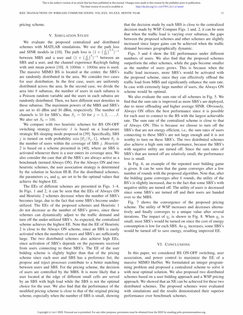
The EEs of different schemes are presented in Figs. 1–4.

In Figs. 1 and 2, it can be seen that the EEs of Always ON

and Heuristic 2 schemes decrease when the number of SBS’s

becomes large, due to the fact that some SBS’s become under-

utilized. The EEs of the proposed schemes and Heuristic 1

do not decrease as the number of SBS’s grows, since these

schemes can dynamically adjust to the traffic demand and

turn off the under-utilized SBS’s. As expected, the centralized

scheme achieves the highest EE. Note that the EE of Heuristic

2 is close to the Always ON scheme, since an SBS is easily

activated when the numbers of users and SBS’s are sufficiently

large. The two distributed schemes also achieve high EEs,

since activation of SBS’s depends on the payments received

from users connecting to these SBS’s. The EE of the user

bidding scheme is slightly higher than that of the pricing

scheme since each user and SBS has a preference list, the

propose and reject processes contribute to a better matching

between users and SBS. For the pricing scheme, the decision

of users are controlled by the MBS. It is more likely that a

user located at the edge of different small cells are served

by an SBS with high load while the SBS is not the optimal

choice for the user. We also find that the performance of the

modified pricing scheme is close to that of the original pricing

scheme, especially when the number of SBS is small, showing

that the decision made by each SBS is close to the centralized

decision made by WSP. Compare Figs. 1 and. 2, it can be seen

that when the traffic load is varying over subareas, the gaps

between the proposed schemes and other schemes are slightly

increased since larger gains can be achieved when the traffic

demand becomes geographically dynamic.

Figs. 3 and 4 show the EE performance under different

numbers of users. We also find that the proposed schemes

outperform the other schemes, while the gaps become smaller

as the number of users grows. This is because when the

traffic load increases, more SBS’s would be activated with

the proposed scheme, since they can effectively offload the

traffic load from MBS and significantly enhance the sum rate.

In case with extremely large number of users, the Always ON

scheme would be optimal.

We also evaluate the sum rate of all schemes in Fig. 5. We

find that the sum rate is improved as more SBS’s are deployed,

due to more offloading and higher average SINR. Obviously,

Always ON offers the best performance since it is possible

for each user to connect to the BS with the largest achievable

rate. The sum rate of the centralized scheme is close to that

of Always ON. This is because we choose to turn off the

SBS’s that are not energy efficient, i.e., the sum rates of users

connecting to these SBS’s are not large enough and it is not

worthy to turn on these SBS’s. The two distributed schemes

also achieve a high sum rate performance, because the SBS’s

with negative utility are turned off. Since the sum rates of

SBS’s that are turned off are relatively small, the performance

loss is small.

In Fig. 6, an example of the repeated user bidding game

is given. It can be seen that the game converges after a few

number of rounds with the proposed algorithm. Note that, after

the bidding game converges after 6 rounds, the utility of the

BS’s is slightly increased, due to the fact that some SBS’s with

negative utility are turned off. The utility of users is decreased

since some SBS’s are turned off and their users are handed

over to the MBS.

Fig. 7 shows the convergence of the proposed pricing

scheme. The utility of WSP increases and decreases alterna-

tively and finally converges to a unique value after several

iterations. The impact of qj is shown in Fig. 8. When qj is

small, most SBS’s would be turned on since the cost of energy

consumption is low for each SBS. As qj increases, some SBS’s

would be turned off to save energy, resulting improved EE.

VI. CONCLUSIONS

In this paper, we considered BS ON-OFF switching, user

association, and power control to maximize the EE of a

massive MIMO HetNet. We formulated an integer program-

ming problem and proposed a centralized scheme to solve it

with near optimal solution. We also proposed two distributed

schemes based on a user bidding approach and a WSP pricing

approach. We showed that an NE can be achieved for these two

distributed schemes. The proposed schemes were evaluated

with simulations and the results demonstrated their superior

performance over benchmark schemes.




5 10 15 204.3

4.4

4.5

4.6

4.7

4.8

4.9

5x 10

6

Number of SBS

Aver

age

ener

gy e

ffic

iency

(bit

s/Jo

ule

)

Centralized

User bidding

Heuristic1

Heuristic2

Always ON

WSP pricing

Modified WSP pricing

Fig. 1. Average system EE versus number of SBS’s for different BS ON-OFFswitching strategies: 100 users, uniformly distributed.

5 10 15 204.3

4.4

4.5

4.6

4.7

4.8

4.9

5

5.1x 10

6

Number of SBS

Aver

age

ener

gy e

ffic

iency

(bit

s/Jo

ule

)

Centralized

User bidding

Heuristic1

Heuristic2

Always ON

WSP pricing


Fig. 2. Average system EE versus number of SBS’s for different BS ON-OFFswitching strategies: 100 users, non-uniformly distributed.

50 100 150 2003.8

4

4.2

4.4

4.6

4.8

5

5.2

5.4

5.6x 10

6

Number of users

Aver

age

ener

gy e

ffic

iency

(bit

s/Jo

ule

)

Centralized

User bidding

Heuristic1

Heuristic2

Always ON

WSP pricing


Fig. 3. Average EE efficiency versus number of users for different BS ON-OFFswitching strategies: uniformly distributed users, 10 SBS’s.

50 100 150 2003.8

4

4.2

4.4

4.6

4.8

5

5.2

5.4

5.6x 10

6

Average number of users

Aver

age

ener

gy e

ffic

iency

(bit

s/Jo

ule

)

Centralized

User bidding

Heuristic1

Heuristic2

Always ON

WSP pricing


Fig. 4. Average system EE versus average number of users for different BSON-OFF switching strategies: non-uniformly distributed users, 10 SBS’s.

5 10 15 202

3

4

5

6

7

8

9

10

11x 10

8

Number of SBS

Aver

age

sum

rat

e (b

ps)

Centralized

User bidding

Heuristic1

Heuristic2

Always ON

WSP pricing


Fig. 5. Average sum rate versus number of SBS’s for different BS OF-OFFswitching strategies: 100 users, uniformly distributed.

0 1 2 3 4 5 6 7 80

0.5

1

1.5

2

2.5

3

3.5

4

Round of game

No

rmali

zed

uti

lity

Sum utility of users

Sum utility of BS’s

Fig. 6. Convergence of the repeated bidding game: 100 users and 10 SBS’s.

REFERENCES

[1] Qualcomm, “The 1000x data challenge,” [online] Available:https://www.qualcomm.com/1000x.

[2] M. Feng and S. Mao, “Harvest the potential of massive MIMOwith multi-layer technologies,” IEEE Network, vol.30, no.5, pp.40–45,Sept./Oct. 2016.

[3] M. Feng, S. Mao, and T. Jiang, “BOOST: Base station on-off switching




0 1 2 3 4 5 6 7 80

1

2

3

4

5

6

Number of iteration

Norm

aliz

ed u

tili

ty o

f W

SP

Fig. 7. Convergence of the iterative pricing scheme: 100 users and 10 SBS’s.

0 5 10 15 20 25 30 35 402

2.5

3

3.5

4

4.5x 10

6

qj

Aver

age

ener

gy e

ffic

iency

(bit

s/Jo

ule

)

User bidding

Fig. 8. Average system EE versus different values of qj : 100 users and 10

SBS’s, pk,j = 1.

strategy for energy efficient massive MIMO HetNets,” in Proc. IEEE

INFOCOM’16, San Francisco, CA, Apr. 2016, pp.1395–1403.

[4] A. Adhikary, H.S. Dhillon, and G. Caire, “Massive-MIMO meetsHetNet: Interference coordination through spatial blanking,” IEEE J.

Select. Areas Commun., vol.33, no.6, pp.1171–1186, June 2015.

[5] K. Zheng, L. Zhao, J. Mei, B. Shao, W. Xiang, and L. Hanzo, “Surveyof large-scale MIMO systems,” IEEE Commun. Sur. & Tut., vol.17, no.3,pp.1738–1760, Third Quarter 2015.

[6] T.L. Marzetta, “Noncooperative cellular wireless with unlimited numbersof base station antennas,” IEEE Trans. Wireless Commun., vol.9, no.11,pp.3590–3600, Nov. 2010.

[7] H.Q. Ngo, E.G. Larsson, and T.L. Marzetta, “Energy and spectral effi-ciency of very large multiuser MIMO systems,” IEEE Trans. Commun.,

vol.61, no.4, pp.1436–1449, Apr. 2013.

[8] Y. Xu, G. Yue, and S. Mao, “User grouping for massive MIMO in FDDsystems: New design methods and analysis,” IEEE Access Journal, vol.2,no.1, pp.947–959, Sept. 2014.

[9] E. Bjornson, M. Kountouris, and M. Debbah, “Massive MIMO and smallcells: Improving energy efficiency by optimal soft-cell coordination,” inProc. ICT’13, Casablanca, Morocco, May 2013, pp.1–5.

[10] D. Bethanabhotla, O.Y. Bursalioglu, H.C. Papadopoulos, and G. Caire,“User association and load balancing for cellular massive MIMO,” inProc. IEEE Inf. Theory Appl. Workshop 2014, San Diego, CA, Feb.2014, pp.1–10.

[11] Y. Xu and S. Mao, “User Association in Massive MIMO HetNets,” IEEE

Systems Journal, vol.11, no.1, pp.7–19, Mar. 2017.

[12] D. Liu, et al., “Distributed energy efficient fair user association inmassive MIMO enabled HetNets,” IEEE Comm. Lett., vol.19, no.10,pp.1770–1773, Oct. 2015.

[13] M. Feng and S. Mao, “Interference management and user association fornested array-based massive MIMO HetNets,” IEEE Trans. Veh. Technol.,

to appear. DOI: 10.1109/TVT.2017.2741900.

[14] M. Feng and S. Mao, “Adaptive pilot design for massive MIMO HetNetswith wireless backhaul,” in Proc. IEEE SECON’17, San Diego, CA, June2017, pp.1–9.

[15] Y. Chen, S. Zhang, S. Xu, and G.Y. Li, “Fundamental tradeoffs on greenwireless networks,” IEEE Commun., vol.49, no.6, pp. 30–37, June 2011.

[16] E. Oh, B. Krishnamachari, X. Liu, and Z. Niu, “Toward dynamic energy-efficient operation of cellular network infrastructure,” IEEE Commun.,

vol.49, no.6, pp.56–61, June 2011.

[17] M. Feng, S. Mao, and T. Jiang, “Base station ON-OFF switchingin 5G wireless networks: Approaches and challenges,” IEEE Wireless

Commun., vol.24, no.4, pp.46–54, Aug. 2017.

[18] V. Chandrasekhar and J.G. Andrews, “Spectrum allocation in tieredcellular networks,” IEEE Trans. Commun., vol.57, no.10, pp.3059–3068,Oct. 2009.

[19] S. Zhang, J. Gong, S. Zhou, and Z. Niu, “How many small cells can beturned off via vertical offloading under a separation architecture?” IEEE

Trans. Wireless Commun., vol.14, no.10, pp.5440–5453, Oct. 2015.

[20] S. Cai, Y. Che, L. Duan, J. Wang, S. Zhou, and R. Zhang, “Green 5Gheterogeneous networks through dynamic small-cell operation,” IEEE J.

Sel. Areas Commun., vol.34, no.5, pp.1103–1115, May 2016.

[21] E. Bjornson, E.G. Larsson, and M. Debbah, “Massive MIMO formaximal spectral effciency: How many users and pilots should beallocated?” IEEE Trans. Wireless Commun., vol.15, no.2, pp.1293–1308,Feb. 2016.

[22] E. Bjornson, L. Sanguinetti, and M. Kountouris, “Deploying densenetworks for maximal energy efficiency: Small cells meet massiveMIMO,” IEEE J. Select. Areas Commun., vol.34, no.4, pp.832–847, Apr.2016.

[23] H. Ngo, H. Suraweera, M. Matthaiou, and E. Larsson, “Multipair full-duplex relaying with massive arrays and linear processing,” IEEE J. Sel.

Areas Commun., vol.32, no.9, pp.1721–1737, June 2014.

[24] D. Bethanabhotla, O.Y. Bursalioglu, H.C. Papadopoulos, and G. Caire,“Optimal user-cell association for massive MIMO wireless networks,”IEEE Trans. Wireless Commun., vol.15, no.3, pp.1835–1850, Mar. 2016.

[25] Q. Ye, O.Y. Bursalioglu, H.C. Papadopoulos, C. Caramanis, and J.G.Andrews, “User association and interference management in massiveMIMO hetNets,” IEEE Trans. Wireless Commun., vol.64, no.5, pp.2049–2065, May 2016.

[26] F. Fernandes, A. Ashikhmin, and T.L. Marzetta, “Inter-cell interferencein noncooperative TDD large scale antenna systems,” IEEE J. Select.

Areas Commun., vol.31, no.2, pp.192–201, Feb. 2013.

[27] N. Wang, E. Hossain, and V.K. Bhargava, “Joint downlink cell as-sociation and bandwidth allocation for wireless backhauling in two-tier hetNets with large-scale antenna arrays,” IEEE Trans. Wireless

Commun., vol.15, no.5, pp.3251–3268, May 2016.

[28] Q. Ye, B. Rong, Y. Chen, M.A.-Shalash, C. Caramanis, and J.G.Andrews, “User association for load balancing in heterogeneous cellularnetworks,” IEEE Trans. Wireless Commun., vol.12, no.6, pp.2706–2716,June 2013.

[29] O. Arnold, F. Richter, G. Fettweis, and O. Blume, “Power consumptionmodeling of different base station types in heterogeneous cellularnetworks,” in Proc. Future Netw. Mobile Summit, Florence, Italy, June2010, pp.1–8.

[30] Y. Huang, et al., “Energy-efficient design in heterogeneous cellularnetworks based on large-scale user behavior constraints,” IEEE Trans.

Wireless Commun., vol.13, no.9, pp.4746–4757, Sept. 2014.

[31] L. Chen, et al., “Green full-duplex self-backhaul and energy harvestingsmall cell networks with massive MIMO,” IEEE J. Sel. Areas Commun.,

vol.34, no.12, pp.3709–3724, Dec. 2016.

[32] E. Oh, K. Son, and B. Krishnamachari, “Dynamic base station switching-on/off strategies for green cellular networks,” IEEE Trans. Wireless

Commun., vol.12, no.5, pp.2126–2136, May 2013.

[33] X. Guo, Z. Niu, S. Zhou, and P.R. Kumar, “Delay-constrained energy-optimal base station sleeping control,” IEEE J. Sel. Areas Commun.,

vol.34, no.5, pp.1073–1085, May 2016.

[34] 3GPP TS 36.420, “Evolved universal terrestrial radio access network(EUTRAN); X2 general aspects and principles,” Dec. 2008.

[35] S. Boyd and L. Vandenberghe, Convex Optimization,, Cambridge Uni-versity Press, 2004.

[36] W. Yu, “Multiuser water-flling in the presence of crosstalk,” in Proc.

IEEE ITA Workshop, San Diego, CA, Jan. 2007, pp.414–420.




[37] A. Schrijver, Theory of Linear and Integer Programming, John Wiley& Sons, June 1998.

[38] C. Berenstein and R. Gay, Complex Variables: An Introduction, Springer,1997.

[39] Y.S. Soh, T.Q.S. Quek, M. Kountouris, and H. Shin, “Energy efficientheterogeneous cellular networks,” IEEE J. Select. Areas Commun.,

vol.31, no.5, pp.840–850, May 2013.[40] I. Ashraf, L.T.W. Ho, and H. Claussen, “Improving energy efficiency of

femtocell base stations via user activity detection,” in Proc. WCNC’10,

Sydney, Austrilia, Apr. 2010, pp.1–5.

Mingjie Feng [S’15] received his B.E. and M.E.degrees from Huazhong University of Science andTechnology in 2010 and 2013, respectively, both inelectrical engineering. He was a visiting student inthe Department of Computer Science, Hong KongUniversity of Science and Technology, in 2013. He iscurrently a Ph.D. student in the Department of Elec-trical and Computer Engineering, Auburn University,AL. His research interests include cognitive radionetworks, heterogeneous networks, massive MIMO,mmWave network, and full-duplex communication.

He is a recipient of a Woltosz Fellowship at Auburn University.

Shiwen Mao [S’99-M’04-SM’09] received hisPh.D. in electrical and computer engineering fromPolytechnic University, Brooklyn, NY in 2004. Heis the Samuel Ginn Distinguished Professor andDirector of the Wireless Engineering Research andEducation Center (WEREC) at Auburn University,Auburn, AL. His research interests include wirelessnetworks and multimedia communications. He isa Distinguished Lecturer of the IEEE VehicularTechnology Society. He received the 2015 IEEEComSoc TC-CSR Distinguished Service Award, the

2013 IEEE ComSoc MMTC Outstanding Leadership Award, and the NSFCAREER Award in 2010. He is a co-recipient of the Best Demo Awardfrom IEEE SECON 2017, the Best Paper Awards from IEEE GLOBECOM2016 & 2015, IEEE WCNC 2015, and IEEE ICC 2013, and the 2004IEEE Communications Society Leonard G. Abraham Prize in the Field ofCommunications Systems.

Tao Jiang [M’06-SM’10] is currently a Chair Pro-fessor in the School of Electronics Information andCommunications, Huazhong University of Scienceand Technology, Wuhan, P. R. China. He receivedPh.D. degree in information and communicationengineering from Huazhong University of Scienceand Technology, Wuhan, P.R. China, in Apr. 2004.He has authored or co-authored over 200 technicalpapers in major journals and conferences and 9books/chapters in the areas of communications andnetworks. He has served or is serving as associate

editor of some technical journals in communications, including in IEEE Trans-actions on Signal Processing, IEEE Communications Surveys and Tutorials,IEEE Transactions on Vehicular Technology, IEEE Internet of Things Journal,and he is the associate editor-in-chief of China Communications. He is arecipient of the NSFC Distinguished Young Scholars Award in 2013. He wasawarded as the Most Cited Chinese Researchers announced by Elsevier in2014, 2015 and 2016. He is a senior member of IEEE.



Documents

IEEE TRANSACTIONS ON WIRELESS …szm0001/papers/TWC2746689.pdfneous network (HetNet) with massive MIMO, ... Switching sTrategy) to maximize the EE of a massive MIMO HetNet, by jointly