Idiosyncratic Return Volatility, Cash Flows, and Product ... · Idiosyncratic Return Volatility, Cash Flows, and Product Market Competition The paper is organized as follows. Section

Idiosyncratic Return Volatility, Cash Flows,and Product Market Competition

Paul J. IrvineTerry College of Business, University of Georgia

Jeffrey PontiffCarroll School of Management, Boston College

Over the past 40 years, the volatility of the average stock return has drastically outpacedtotal market volatility. Thus, idiosyncratic return volatility has dramatically increased. Weestimate this increase to be 6% per year. Consistent with an efficient market, this resultis mirrored by an increase in the idiosyncratic volatility of fundamental cash flows. Weargue that these findings are attributable to the more intense economy-wide competition.Various cross-sectional and time-series tests support this idea. Economic competitivenessfacilitates reinterpretation of the results from the cross-country R2 literature, as well as theUS idiosyncratic risk literature. (JEL G12, G14).

Idiosyncratic stock-return volatility varies across countries as well as throughtime. Morck, Yeung, and Yu (2000) focus on cross-country differences inmarket model return R2s, and show that stock-return R2s are higher in countrieswith more opaque information environments. Campbell et al. (2001) reportthat stock-return volatility increased dramatically over the 1962–1997 period,although aggregate market volatility did not change during this time period,implying that the idiosyncratic risk of the typical stock has increased.

In a rational market, stock prices equate to the present value of future-expected cash flows. This basic formulation yields three fundamental expla-nations for both cross-country differences and the time trend in idiosyncraticrisk: (1) discount rate shocks increase idiosyncratic return volatility; (2) cash-flow streams have become more idiosyncratic; or (3) the market is inefficient.The first explanation is not very persuasive, since on theoretical grounds it isquestionable whether discount rate news can cause idiosyncratic risk. Discountrate shocks are determined by the true asset pricing model. Modern risk-basedasset pricing theories (e.g., Sharpe, 1964) maintain that idiosyncratic risk isnot priced, and thus the source of idiosyncratic return variation is not a risk

We thank Randy Becker, Pierluigi Balduzzi, Sam Choi, John Campbell, David Chapman, Wayne Ferson, EdieHotchkiss, Jeffry Netter, Ed Rice, Matt Spiegel, Yexiao Xu, and seminar participants at Boston College, Cornell,Drexel, Georgia, Ohio State, UNLV, and the 2005 Western Finance Association Annual Meeting for helpfulcomments. We also thank Jim Linck for providing additional historical segment data, and Yong Chen, RonHarris, Karthik Krishnan, and Ivonne Moya for research assistance. Send correspondence to Paul Irvine, TerryCollege of Business, University of Georgia, Athens, GA, 30602. E-mail: [email protected].

C© The Author 2008. Published by Oxford University Press on behalf of The Society for Financial Studies.All rights reserved. For Permissions, please e-mail: [email protected]:10.1093/rfs/hhn039 Advance Access publication April 15, 2008

The Review of Financial Studies / v 22 n 3 2009

factor. Of course, the parameters of the underlying asset pricing model could besubject to idiosyncratic variation that, in turn, causes idiosyncratic shocks tostock returns. For example, in the case of the capital asset pricing model(CAPM), variation in beta could create idiosyncratic changes in discount rates,which are then reflected in idiosyncratic return risk. Since Campbell et al.(2001) examine monthly risk measures using daily data, this explanation seemsimplausible, since it requires drastic intramonth parameter variation.

The two remaining fundamental explanations are either that idiosyncraticnews in cash flows is sufficient to explain the trend of higher idiosyncraticvolatility or that the market is inefficient, or both. The first goal of our paper isto examine the US time series of idiosyncratic volatility to assess these explana-tions. Using various measures of fundamental cash-flow volatility, we find thatthe trend in idiosyncratic cash-flow volatility mirrors the trend in idiosyncraticstock-return volatility, consistent with market efficiency. Idiosyncratic returnvolatility forecasts idiosyncratic cash-flow volatility in the following two quar-ters. This finding leads to another quandary: What has changed in the economyto make firms subject to greater idiosyncratic risk in fundamental cash flows?Our second goal is to investigate explanations for this puzzling trend.

The mosaic of evidence suggests that the recent upward trend in idiosyncraticvolatility is related to an increasingly competitive environment in which firmshave less market power. When the success of one firm in an industry comes atthe expense of another firm in that industry, competition contributes to negativecovariance in firm performance. In general, markets reflect an environmentwith less consumer loyalty to a specific firm, perhaps due to better access toinformation or the reduction of other search costs. Our results coincide withthe findings of economics research that indicates increased competition in theUS economy (e.g., Blinder, 2000; London, 2004; and Bils and Klenow, 2004).

Our finding of a relation of between idiosyncratic stock-return volatility andfundamental volatility, as well as our associating this effect with increased com-petition, provides a new interpretation of evidence from international studiessuch as Morck, Yeung, and Yu (2000). We recognize that opaque informa-tion deters a country’s product-market competition. We offer a challenge to theconclusion that information opacity affects stock-return R2s through stock trad-ing. Rather, we argue that information opacity affects a country’s fundamentalbusiness environment, which in turn affects stock-return R2s.

Our findings offer new evidence on the importance of financial market inno-vation with regard to economic advancement. Brown and Kapadia (2007) claimthat the increase in idiosyncratic risk is related to more volatile firms being listedthrough initial public offerings, and Bennett and Sias (2006) show that the pro-portion of firms with small market capitalizations has increased. In light ofthese studies, our finding of an association between idiosyncratic risk and eco-nomic competitiveness leads to an interesting conjecture—financial innovationallows small, risky firms to raise capital, thus inducing greater economy-widecompetition.

1150

Idiosyncratic Return Volatility, Cash Flows, and Product Market Competition

The paper is organized as follows. Section 1 describes the sample and dis-cusses our measure of earnings volatility. Section 2 replicates the results ofCampbell et al. (2001) for the intersection of firms in the Center for Researchin Security Prices (CRSP) and Compustat databases. Section 3 examines theidiosyncratic volatility of earnings, cash flows, and sales over time. Section 4examines increased competitiveness (including deregulation) as an explanationfor increased idiosyncratic volatility, and Section 5 concludes.

1. Framework and Data

Since our investigation focuses on the direct link between cash-flow shocksand return volatility, we first outline the link between these two variables witha simple one-period model of stock returns. Specifically,

p0 =∞∑

i=1

E0(C Fi )

(1 + k)i, (1)

where CFi is the cash flow at time i, k is the appropriate discount rate, andE0 (·) is the expectations operator as of time 0. If cash flows follow a randomwalk, then

E0 (C Fi ) = C F0, ∀i ≥ 0. (2)

Equations (1) and (2) imply that

p0 = C F0

k. (3a)

Similarly,

p1 = C F1

k= C F0 + e1

k. (3b)

In this case, e1 is the random unexpected cash-flow shock at time 1. Therealized return at time 1 is then a random variable given by

r1 = p1 − p0

p0= e1

kp0, (4)

with variance

σ2 (r1) = σ2 (e1)

k2 p20

. (5)

Since k and p0 are predetermined at time 0, the source of the variance ofthe stock-return process comes directly from the variance of unexpected cash

1151


flows. This analysis implies that a comparison of cash-flow shock variabilityto stock market return variability necessitates the use of a cash-flow shock thatis scaled by the product of the price and the discount rate.

A recent study by Wei and Zhang (2006) compares idiosyncratic stock marketvolatility to the volatility of the level of earnings divided by the book value ofshareholder equity. This comparison does not directly illustrate the source ofcash-flow volatility, since return volatility is determined by unexpected shocksto the cash-flow stream, not by the cash-flow stream itself. Scaling by the bookvalue of equity instead of price adds noise to the variance estimation, the bias orimpact of which is unclear. Inference from their results is also impeded by thefact that they present evidence of total rather than idiosyncratic ROE volatility.Comin and Philippon (2005) examine sales growth volatility. Their measure isan improvement on Wei and Zhang (2006) in that they do not scale by bookvalue, although like Wei and Zhang (2006), the idiosyncratic component of riskis left unexamined.

1.1 CRSP-Compustat databaseOur data come from the intersection of the CRSP/Compustat merged databases.In general, Compustat coverage is a subset of CRSP coverage. We must furtherlimit our data as the persistence in time-series accounting data in our analysisof idiosyncratic cash-flow shocks requires at least twelve consecutive quartersof Compustat data for each firm in the sample. For each firm, we also requirethat each quarter have all of the following Compustat data items: sales (2),depreciation and amortization (5), end-of-quarter stock price (14), number ofcommon shares used to calculate earnings per share (15), and earnings pershare excluding extraordinary items (19).

The empirical analysis of cash-flow volatility examines three separate cash-flow measures: (i) earnings per share, for which we use Compustat data item19; (ii) cash flow per share, which we compute by adding depreciation (dataitem 5) per share to earnings per share; and (iii) sales per share, for whichwe divide Compustat data item 2 by data item 15. We expect that these threemeasures should sufficiently reflect any fundamental cash-flow shocks affectinga corporation.

To alleviate the effect of outliers, we winsorize the data. We first divideper-share earnings, cash flows, and sales by price. If the resulting value of anyof these three variables is above (below) its respective top (bottom) percentile,we assign to it the value of the observation at the top (bottom) percentile, andthen retransform the variable by multiplying by price. This procedure enablesus to limit the effect of potentially misleading accounting numbers, without themeasurement error sometimes associated with firms with extreme stock-pricelevels. Table 1 presents winsorized summary information on the sample firms.1

1 In unreported results, we simply delete the outliers instead of winsorizing them and obtain lower point estimatesof the growth in idiosyncratic volatility for all cash-flow proxies. Significance of these estimates is similar to that

1152


Table 1Univariate sample statistics

N Mean σ 25th percentile Median 75th percentile

Earnings per share ($) 577,322 0.19 0.92 −0.03 0.11 0.40Cash-flow per share ($) 577,315 0.44 1.40 0.00 0.25 0.68Sales per share (million dollars) 577,315 6.35 14.96 0.70 2.84 7.30Earnings-to-price 577,322 −0.02 0.14 −0.01 0.01 0.02Cash-flow-to-price 577,315 0.01 0.12 0.00 0.02 0.04Sales-to-price 577,315 0.61 1.06 0.10 0.26 0.63

Aggregate statistics for earnings, cash flow, and sales on the CRSP-Compustat merged database, 1962–2003. If the ratio of any of these three variables divided by price is in the top or bottom 1% of thedistribution, the variable is winsorized by setting the price-normalized value equal to the appropriate1% value and then multiplying by price.

1.2 Measuring earnings shocksBrown and Rozeff (1979), and Brown (1993) report that the levels of accountingmeasures of cash flows exhibit persistence. To measure the unexpected cash-flow shock correctly in our accounting measures of cash flows, we need tocontrol for the documented persistence in cash flows. A preliminary empiricalanalysis of our data reveals that all three of our cash-flow measures demonstratestrong time-series persistence. We therefore focus on the differences of thesecash-flow variables as the correct measure of innovations in each series. Asthe residuals of the differences can still exhibit some persistence, as well asseasonal variation, we estimate the following pooled cross-sectional time-seriesmodel:

Eit − Eit−4 = α + β1(Eit−1 − Eit−5) + β2(Eit−2 − Eit−6)

+ β3 (Eit−3 − Eit−7) + eit . (6)

This model is estimated at the industry level for each of the 49 Fama-French(1997) industry groups, thus allowing intercepts and slopes to vary dependingon the industry. The Eit are vectors of either firm-level earnings, cash flows,or sales at quarter t. In this model, the residuals eit are vectors of unexpectedinnovations in a firm’s cash flow per share. The dependent variable is thedifference between the current quarter’s earnings and the earnings that werereported in the same quarter of the preceding year.

The primary advantage of the estimation in Equation (6) is that it imposesonly limited restrictions on the firm-level residuals. For any particular firm, theunexpected cash-flow innovations do not have to sum to zero, so the modelpermits a firm to outperform or underperform over time. Also, at any pointin time, the cross-sectional vector of unexpected innovations to earnings pershare does not have to sum to zero, so the model permits all firms to outperform(underperform) the model’s benchmark if economic conditions are particularlystrong (weak) in that period.

reported below in Table 3 (earnings and cash-flow idiosyncratic volatility are statistically significant), whereasthe trend in idiosyncratic sales volatility is weaker.

1153


Estimation of Equation (6) requires that up to nine lags of earnings existin the CRSP-Compustat database. This constraint reduces the sample sizefrom approximately 577,300 firm-specific observations reported in Table 1to approximately 469,000 firm-specific observations. Due to cross-sectionalvariation in the number of missing Compustat data items, the reported numberof observations is slightly different for earnings, cash flow, and sales.

We use the residuals from Equation (6) to calculate idiosyncratic cash-flowshocks at time t. For each firm quarter, we divide its Equation (6) residual bythe end-of-quarter stock price in the previous quarter. Ideally, we would alsoscale earnings by the discount rate as in Equation (4). However, since discountrates must be estimated, scaling by discount rates would introduce noise to ourcash-flow shock measures.

1.3 EstimationUsing our sample of firms with data in both CRSP and Compustat, we constructa daily equal-weighted index. This index is used to compute monthly totalmarket variance from daily return data. Specifically,

σ (ret)2mt =

(n

n − 1

) n∑s=1

(Rms − um)2, (7)

where σ2mt is our estimate for monthly variance, s corresponds to days within

a month, n is the total number of days in a given month, Rms is the dailyreturn of the equal-weighted market index, and um is the average daily returnof the index for month m. We examine equal-weighted idiosyncratic volatilityas opposed to value-weighted idiosyncratic volatility for two reasons. First,if idiosyncratic volatility is caused by trading behavior that is not related tofundamentals, then it should be easier to observe in stocks that have smallmarket capitalizations. These stocks have higher transaction costs, so rationalinvestors will be less likely to induce corrective price pressure (Pontiff, 1996).Second, we are concerned with examining the association between competitionand idiosyncratic volatility. Value weighting is less likely to reflect the conditionof more competitive companies, since the present value of monopoly rents willbe reflected in market values. However, the results (available from the authors)are similar when we use a value-weighted estimation.

Similarly, our monthly idiosyncratic risk measure is estimated from

σ(ret)2Idio,t = 1

j

(n

n − 1

) j∑i=1

n∑s=1

(Ris − Rms)2, (8)

where j is the total number of firms represented in a given month and n isthe number of days in a given month. Campbell et al. (2001) show that thismeasure of idiosyncratic volatility is very close to the idiosyncratic volatil-ity that one can measure from a market model. The advantage of using

1154


Equation (8) to measure idiosyncratic volatility is that it does not requireestimation of beta.

Computation of idiosyncratic cash-flow volatility is analogous. First, wecreate an equal-weighted index of monthly cash-flow shocks. Because firms’fiscal periods vary, a different sample of firms report quarterly earnings in aparticular month. We address nonsynchronicity in the cash-flow reporting byconstructing an index that includes cash-flow shocks from the previous month,the current month, and the following month. Therefore, our index is a rollingaverage of all firms’ cash-flow shocks. Denoting the market cash-flow shockindex in month t as emt, and the cash-flow shock of firm i at time t as eit, amonthly index of the idiosyncratic volatility of cash-flow shocks is constructedas follows:

σ2 (C F)Idio,t =(

1

3

) (1

k

) k∑i=1

(π

2

)(eit − emt)

2, (9)

where k is the total number of firms that report earnings at time t, time t − 1,or time t + 1. Similarly, eit is firm i’s cash-flow shock at time t. If time t doesnot correspond to the end of the firm’s quarter, eit reflects either the quarterlycash flow that was announced in the previous month or the quarterly cash flowthat was announced in the following month. Assuming that eit − emt has a zeromean, multiplying the squared deviation by π

2 gives us an estimate of the firm’sidiosyncratic volatility at time t.2 Since our earnings data are quarterly andwe compare our estimate to monthly stock returns, we multiply our estimateof average idiosyncratic cash-flow risk by 1/3, to produce a monthly estimate.This procedure produces a rolling time-series estimate of monthly fundamentalvolatility, analogous to Campbell et al.’s (2001) calculation of idiosyncraticreturn volatility, from January 1964 through December 2003. The resultingtime series consists of 480 months of idiosyncratic volatility of earnings, cashflows, and sales.

2. Idiosyncratic Return Volatility in the CRSP-Compustat Merged Data

Our three cash-flow measures require Compustat data, thus restricting our datato a subset of the sample used by Campbell et al. (2001). To ensure that theresults obtained from our sample are relevant to the conclusions in Campbellet al., we first examine whether idiosyncratic volatility increases over time inour subsample.

We estimate idiosyncratic volatility for the CRSP-Compustat sample by cal-culating market-adjusted abnormal returns for each firm month and estimating

2 Schwert and Seguin (1990) estimate the volatility of monthly returns in a similar fashion. Equation (9) uses thefact that the formula for the absolute value of a normally distributed variable contains a standard deviation termand the fact that the sample-wide mean of eit is equal to zero.

1155


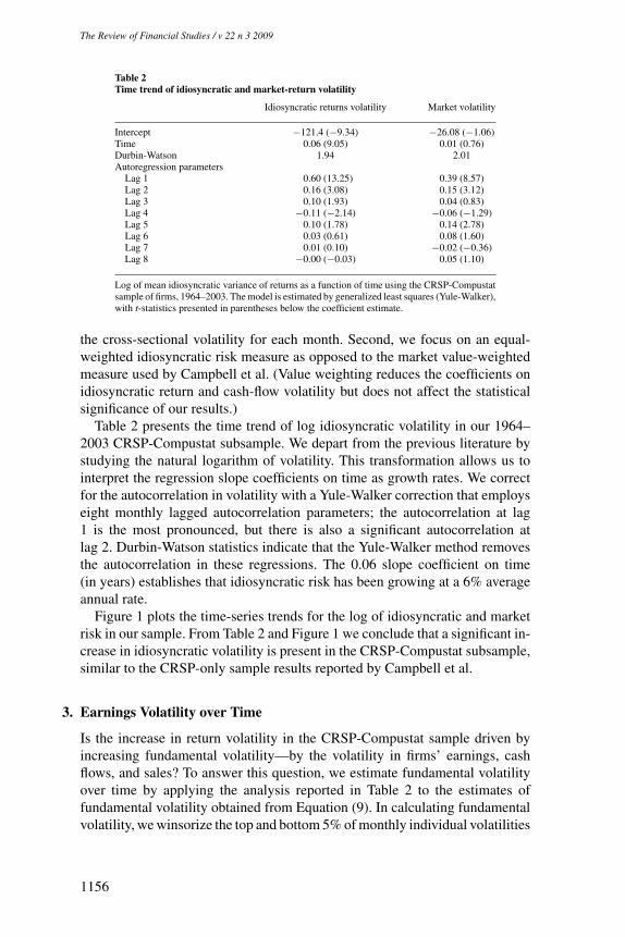
Table 2Time trend of idiosyncratic and market-return volatility

Idiosyncratic returns volatility Market volatility

Intercept −121.4 (−9.34) −26.08 (−1.06)Time 0.06 (9.05) 0.01 (0.76)Durbin-Watson 1.94 2.01Autoregression parameters

Lag 1 0.60 (13.25) 0.39 (8.57)Lag 2 0.16 (3.08) 0.15 (3.12)Lag 3 0.10 (1.93) 0.04 (0.83)Lag 4 −0.11 (−2.14) −0.06 (−1.29)Lag 5 0.10 (1.78) 0.14 (2.78)Lag 6 0.03 (0.61) 0.08 (1.60)Lag 7 0.01 (0.10) −0.02 (−0.36)Lag 8 −0.00 (−0.03) 0.05 (1.10)

Log of mean idiosyncratic variance of returns as a function of time using the CRSP-Compustatsample of firms, 1964–2003. The model is estimated by generalized least squares (Yule-Walker),with t-statistics presented in parentheses below the coefficient estimate.

the cross-sectional volatility for each month. Second, we focus on an equal-weighted idiosyncratic risk measure as opposed to the market value-weightedmeasure used by Campbell et al. (Value weighting reduces the coefficients onidiosyncratic return and cash-flow volatility but does not affect the statisticalsignificance of our results.)

Table 2 presents the time trend of log idiosyncratic volatility in our 1964–2003 CRSP-Compustat subsample. We depart from the previous literature bystudying the natural logarithm of volatility. This transformation allows us tointerpret the regression slope coefficients on time as growth rates. We correctfor the autocorrelation in volatility with a Yule-Walker correction that employseight monthly lagged autocorrelation parameters; the autocorrelation at lag1 is the most pronounced, but there is also a significant autocorrelation atlag 2. Durbin-Watson statistics indicate that the Yule-Walker method removesthe autocorrelation in these regressions. The 0.06 slope coefficient on time(in years) establishes that idiosyncratic risk has been growing at a 6% averageannual rate.

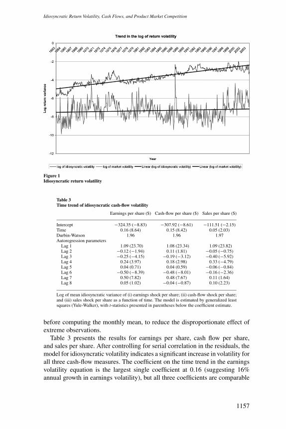
Figure 1 plots the time-series trends for the log of idiosyncratic and marketrisk in our sample. From Table 2 and Figure 1 we conclude that a significant in-crease in idiosyncratic volatility is present in the CRSP-Compustat subsample,similar to the CRSP-only sample results reported by Campbell et al.

3. Earnings Volatility over Time

Is the increase in return volatility in the CRSP-Compustat sample driven byincreasing fundamental volatility—by the volatility in firms’ earnings, cashflows, and sales? To answer this question, we estimate fundamental volatilityover time by applying the analysis reported in Table 2 to the estimates offundamental volatility obtained from Equation (9). In calculating fundamentalvolatility, we winsorize the top and bottom 5% of monthly individual volatilities

1156


Figure 1Idiosyncratic return volatility

Table 3Time trend of idiosyncratic cash-flow volatility

Earnings per share ($) Cash-flow per share ($) Sales per share ($)

Intercept −324.35 (−8.83) −307.92 (−8.61) −111.51 (−2.15)Time 0.16 (8.64) 0.15 (8.42) 0.05 (2.03)Durbin-Watson 1.96 1.96 1.97Autoregression parameters

Lag 1 1.09 (23.70) 1.08 (23.34) 1.09 (23.82)Lag 2 −0.12 (−1.94) 0.11 (1.81) −0.05 (−0.75)Lag 3 −0.25 (−4.15) −0.19 (−3.12) −0.40 (−5.92)Lag 4 0.24 (3.97) 0.18 (2.98) 0.33 (−4.79)Lag 5 0.04 (0.71) 0.04 (0.59) −0.06 (−0.84)Lag 6 −0.50 (−8.39) −0.48 (−8.01) −0.16 (−2.36)Lag 7 0.50 (7.82) 0.48 (7.67) 0.11 (1.64)Lag 8 0.05 (1.02) −0.04 (−0.87) 0.10 (2.23)

Log of mean idiosyncratic variance of (i) earnings shock per share; (ii) cash-flow shock per share;and (iii) sales shock per share as a function of time. The model is estimated by generalized leastsquares (Yule-Walker), with t-statistics presented in parentheses below the coefficient estimate.

before computing the monthly mean, to reduce the disproportionate effect ofextreme observations.

Table 3 presents the results for earnings per share, cash flow per share,and sales per share. After controlling for serial correlation in the residuals, themodel for idiosyncratic volatility indicates a significant increase in volatility forall three cash-flow measures. The coefficient on the time trend in the earningsvolatility equation is the largest single coefficient at 0.16 (suggesting 16%annual growth in earnings volatility), but all three coefficients are comparable

1157


Figure 2Idiosyncratic fundamental volatility

to or larger than the coefficient on the time trend (0.06) in the idiosyncraticreturns volatility regression in Table 2.

Figure 2 plots the time series of all three measures of fundamental idiosyn-cratic volatility over the sample period. The scale of the growth in fundamentalvolatility is large enough to explain the growth in the volatility of idiosyncraticreturns. If anything, the market seems to underreact relative to the idiosyn-cratic volatility in cash flows. This finding has important implications for thetrading-based behavioral explanations of the increase in idiosyncratic volatility.For example, the activity of retail traders, characterized by the rapid increaseof day-trading activity in the 1990s, has been proffered as an explanation forincreased return volatility (Brandt, Brav, and Graham, 2005). Along these lines,Chordia, Roll, and Subrahmanyam (2001) suggest that declining transactioncosts are responsible for increased volatility and volume.

In contrast to the day-trading argument, several papers suggest that institu-tions are more strongly associated with increased idiosyncratic volatility thanare individual investors. Malkiel and Xu (2003) and Dennis and Strickland(2004) find a positive cross-sectional relation between idiosyncratic volatilityand institutional ownership. Malkiel and Xu interpret these results as sug-gesting that institutional trading causes idiosyncratic risk. Bennett, Sias, and

1158


Starks (2003) contend that institutional investors’ changing preferences forsmall stocks have contributed to greater idiosyncratic volatility, particularly forsmall stocks.

Our results suggest that the trend in idiosyncratic fundamental volatility issufficient to explain the increase in idiosyncratic stock-return volatility. Thus,appeals to trading-based explanations are unnecessary. Since it is unlikelythat institutional trading causes higher fundamental volatility, we assert thatinstitutional turnover responds to idiosyncratic volatility—i.e., the causal linkbetween institutional ownership and idiosyncratic volatility runs in the oppositedirection to that put forth by Malkiel and Xu (2003) and Dennis and Strickland(2004). Furthermore, in light of Malkiel and Xu’s Granger causality test, ourresults imply that institutional trading anticipates future changes in idiosyn-cratic volatility. Our explanation is consistent with the paradigm that the roleof some financial institutions such as mutual funds is to provide economiesof scale for investors seeking diversification. If so, these financial institutionsshould hold more idiosyncratic firms, since they have a comparative advantagein managing large portfolios.

3.1 The influence of firm compositionOne explanation for the increase in idiosyncratic risk is that Compustat-CRSPcoverage has changed. Perhaps rather than firms becoming more volatile, morevolatile firms have entered the sample. Such a finding might coincide with therelaxation of the requirements needed for a firm to list on an exchange (Brownand Kapadia, 2007).

We investigate four versions of this explanation. First, is the increase involatility attributable to a larger proportion of smaller firms? Second, has therebeen an increase in the proportion of firms in more volatile industries? Third,irrespective of size and industry, are new listings or new data coverage thesource of the increase in volatility? Fourth, to what extent can the increase involatility be attributable to a trend toward less firm-level diversification?

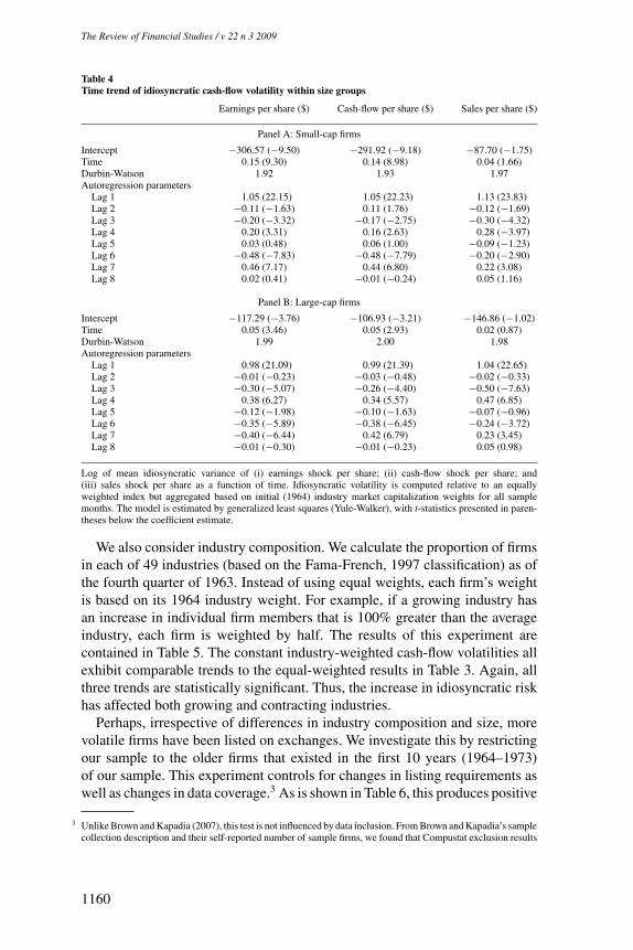
For the first investigation we separate all firms into a small and large marketcapitalization sample. Inclusion into these samples depends on whether thefirm has market capitalization that is greater or less than the inflation-adjustedmedian market capitalization for the sample in the fourth quarter of 1963. Iflisting requirements have enabled smaller firms to list, this methodology wouldleave the large market capitalization sample unaffected since it is determinedby the market capitalization distribution in the beginning of the sample. PanelA of Table 4 shows that the small firm sample has an increase in idiosyncraticcash flows that is similar to that of the full sample, although idiosyncratic salesvolatility is now insignificant. Panel B shows that the large firms still have anincrease in idiosyncratic volatility that is lower than that of small firms, butthe increase in large-firm idiosyncratic volatility is statistically significantly forboth earnings and cash flows.

1159


Table 4Time trend of idiosyncratic cash-flow volatility within size groups


Panel A: Small-cap firms


Lag 1 1.05 (22.15) 1.05 (22.23) 1.13 (23.83)Lag 2 −0.11 (−1.63) 0.11 (1.76) −0.12 (−1.69)Lag 3 −0.20 (−3.32) −0.17 (−2.75) −0.30 (−4.32)Lag 4 0.20 (3.31) 0.16 (2.63) 0.28 (−3.97)Lag 5 0.03 (0.48) 0.06 (1.00) −0.09 (−1.23)Lag 6 −0.48 (−7.83) −0.48 (−7.79) −0.20 (−2.90)Lag 7 0.46 (7.17) 0.44 (6.80) 0.22 (3.08)Lag 8 0.02 (0.41) −0.01 (−0.24) 0.05 (1.16)

Panel B: Large-cap firms


Lag 1 0.98 (21.09) 0.99 (21.39) 1.04 (22.65)Lag 2 −0.01 (−0.23) −0.03 (−0.48) −0.02 (−0.33)Lag 3 −0.30 (−5.07) −0.26 (−4.40) −0.50 (−7.63)Lag 4 0.38 (6.27) 0.34 (5.57) 0.47 (6.85)Lag 5 −0.12 (−1.98) −0.10 (−1.63) −0.07 (−0.96)Lag 6 −0.35 (−5.89) −0.38 (−6.45) −0.24 (−3.72)Lag 7 −0.40 (−6.44) 0.42 (6.79) 0.23 (3.45)Lag 8 −0.01 (−0.30) −0.01 (−0.23) 0.05 (0.98)

Log of mean idiosyncratic variance of (i) earnings shock per share; (ii) cash-flow shock per share; and(iii) sales shock per share as a function of time. Idiosyncratic volatility is computed relative to an equallyweighted index but aggregated based on initial (1964) industry market capitalization weights for all samplemonths. The model is estimated by generalized least squares (Yule-Walker), with t-statistics presented in paren-theses below the coefficient estimate.

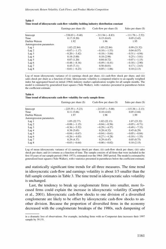
We also consider industry composition. We calculate the proportion of firmsin each of 49 industries (based on the Fama-French, 1997 classification) as ofthe fourth quarter of 1963. Instead of using equal weights, each firm’s weightis based on its 1964 industry weight. For example, if a growing industry hasan increase in individual firm members that is 100% greater than the averageindustry, each firm is weighted by half. The results of this experiment arecontained in Table 5. The constant industry-weighted cash-flow volatilities allexhibit comparable trends to the equal-weighted results in Table 3. Again, allthree trends are statistically significant. Thus, the increase in idiosyncratic riskhas affected both growing and contracting industries.

Perhaps, irrespective of differences in industry composition and size, morevolatile firms have been listed on exchanges. We investigate this by restrictingour sample to the older firms that existed in the first 10 years (1964–1973)of our sample. This experiment controls for changes in listing requirements aswell as changes in data coverage.3 As is shown in Table 6, this produces positive

3 Unlike Brown and Kapadia (2007), this test is not influenced by data inclusion. From Brown and Kapadia’s samplecollection description and their self-reported number of sample firms, we found that Compustat exclusion results

1160


Table 5Time trend of idiosyncratic cash-flow volatility holding industry distribution constant



Lag 1 1.02 (22.84) 1.05 (22.84) 0.99 (21.52)Lag 2 −0.07 (−1.17) −0.10 (−1.53) 0.04 (0.57)Lag 3 −0.20 (−3.42) −0.18 (−3.04) −0.31 (−4.94)Lag 4 0.18 (3.00) 0.18 (2.98) 0.25 (−3.81)Lag 5 0.07 (1.20) 0.04 (0.72) −0.07 (−1.15)Lag 6 −0.48 (−8.16) −0.49 (−8.41) −0.18 (−2.90)Lag 7 0.45 (7.11) 0.50 (8.01) 0.17 (−2.63)Lag 8 −0.01 (−0.23) −0.05 (−1.06) 0.10 (2.13)

Log of mean idiosyncratic variance of (i) earnings shock per share; (ii) cash-flow shock per share; and (iii)sales shock per share as a function of time. Idiosyncratic volatility is computed relative to an equally weightedindex but aggregated based on initial (1964) industry market capitalization weights for all sample months. Themodel is estimated by generalized least squares (Yule-Walker), with t-statistics presented in parentheses belowthe coefficient estimate.

Table 6Time trend of idiosyncratic cash-flow volatility for early sample firms



Lag 1 1.05 (22.77) 1.02 (22.13) 1.07 (23.32)Lag 2 −0.08 (−1.15) −0.04 (−0.56) −0.05 (−0.71)Lag 3 −0.36 (−5.52) −0.29 (−4.57) −0.49 (−7.33)Lag 4 0.38 (5.65) 0.28 (4.32) 0.45 (6.29)Lag 5 −0.04 (−0.67) −0.04 (−0.61) −0.05 (−0.84)Lag 6 −0.26 (−4.03) −0.27 (−4.28) −0.10 (−1.55)Lag 7 0.29 (4.37) 0.29 (4.47) 0.05 (0.75)Lag 8 −0.03 (−0.64) −0.00 (−0.02) 0.10 (2.15)

Log of mean idiosyncratic variance of (i) earnings shock per share; (ii) cash-flow shock per share; (iii) salesshock per share; and (iv) returns as a function of time. The sample consists of all firms that were included in thefirst 10 years of our sample period (1964–1973), estimated over the 1964–2003 period. The model is estimated bygeneralized least squares (Yule-Walker), with t-statistics presented in parentheses below the coefficient estimate.

and statistically significant time trends for all three measures. The time trendin idiosyncratic cash-flow and earnings volatility is about 1/3 smaller than thefull sample estimates in Table 3. The time trend in idiosyncratic sales volatilityis unchanged.

Last, the tendency to break up conglomerate firms into smaller, more fo-cused firms could explain the increase in idiosyncratic volatility (Campbellet al., 2001). Idiosyncratic cash-flow shocks to one division of a diversifiedconglomerate are likely to be offset by idiosyncratic cash-flow shocks to an-other division. Because the proportion of diversified firms in the economydecreased with the conglomerate breakups of the 1980s, such dampening of

in a dramatic loss of observations. For example, including firms with no Compustat data increases their 1997sample by 39.1%.

1161


typical firm volatility should have become less prevalent, resulting in higheraverage idiosyncratic volatility.

We test whether the breakup of diversified firms explains our results byexamining the change in fundamental volatility over time for firms with andwithout multiple lines of business. Lines of business can be obtained fromthe Compustat Industrial Segment database. We obtain the number of businesssegments for the period 1980–2002.4 Unfortunately, the data are disrupted byFinancial Accounting Standards Board Statement (FASB) No. 131, issued in1997, on the reporting of segment information. FASB 131 changed the focusof segment reporting from industries to internal reporting lines. As a result, thereported number of business segments increased and the reported number ofsingle-segment firms initially decreased precipitously (Berger and Hann, 2003).Because of this structural break, the segment data are unreliable after 1997,and we thus analyze only the 1980–1997 time series of business information.

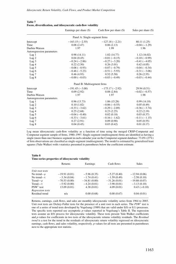
Table 7 examines idiosyncratic cash-flow volatility over the 1980–1997 pe-riod for single-segment and multisegment firms separately. We find that id-iosyncratic volatility increased significantly for both single-segment and mul-tisegment firms. Over this subperiod, the coefficients on the time trend ofearnings and cash flow are significant, and comparable for both types of firms,though the sales coefficient is insignificant. These findings are consistent withRoll (1988), who constructs portfolios of smaller firms to match NYSE andAMEX firms in aggregate size; Roll’s portfolios exhibit much larger R2s thantheir corresponding size-matched firms, indicating that diversification fails toexplain larger firms’ higher observed R2s.

3.2 Time-series propertiesTable 3 reports that all three cash-flow series have large and persistent auto-correlation coefficients, suggesting that the series might be integrated and,therefore, our conclusions could be based on inappropriate test statistics.Table 8 investigates whether our conclusions are appropriate given the time-series properties of idiosyncratic cash flows and returns.

Table 8 presents three different time-series tests. The unit root tests areDickey-Fuller test statistics for each series. The “no trend” results model eachseries as following a first-order autoregressive process with no trend, whereasthe “trend” results incorporate a time trend in the autoregressive process. Sincewe expect a trend in our series, we expect the “no trend” results to provide thestrongest support for a unit root. This is in fact the case that two separate testson the first-order autoregressive series fail to reject the hypothesis of a unit rootfor idiosyncratic earnings and cash flows, although the tests reject the null foridiosyncratic sales volatility. Alternatively, when the time-series specificationcontains a trend, the hypothesis that the series contains a unit root is strongly

4 Business segment data begin in 1978, although Compustat reports a rolling 19-year window, dropping olderyears as new years are added, so currently the oldest reported year is 1985. With the help of other researcherswe were able to recover data going back to 1980.

1162


Table 7Focus, diversification, and idiosyncratic cash-flow volatility

Earnings per share ($) Cash flow per share ($) Sales per share ($)

Panel A: Single-segment firms

Intercept −163.15 (−2.55) −127.18 (−2.21) 80.11 (1.25)Time 0.08 (2.47) 0.06 (2.13) −0.04 (−1.29)Durbin-Watson 1.97 1.99 1.96Autoregression parameters

Lag 1 0.98 (14.11) 1.02 (14.77) 1.12 (16.02)Lag 2 0.04 (0.45) −0.01 (−0.15) −0.10 (−0.99)Lag 3 −0.24 (−2.86) −0.27 (−3.20) −0.41 (−4.05)Lag 4 0.22 (2.50) 0.26 (3.01) 0.42 (4.05)Lag 5 −0.08 (−0.93) −0.07 (−0.79) −0.04 (−0.34)Lag 6 −0.46 (−5.23) −0.51 (−5.93) −0.31 (−3.06)Lag 7 0.46 (4.93) 0.52 (5.58) 0.26 (2.55)Lag 8 −0.00 (−0.03) −0.03 (−0.49) −0.03 (−0.44)

Panel B: Multisegment firms

Intercept −191.45 (−3.00) −175.17 (−2.92) 29.94 (0.51)Time 0.09 (2.92) 0.08 (2.84) −0.02 (−0.57)Durbin-Watson 1.97 1.97 1.98Autoregression parameters

Lag 1 0.96 (13.73) 1.06 (15.28) 0.99 (14.18)Lag 2 0.10 (1.02) −0.06 (−0.55) 0.05 (0.49)Lag 3 −0.33 (−3.62) −0.29 (−2.89) −0.36 (−3.74)Lag 4 0.25 (2.68) 0.23 (2.25) 0.22 (2.19)Lag 5 −0.04 (−0.40) 0.02 (0.18) 0.03 (0.37)Lag 6 −0.33 (−3.61) −0.16 (−1.62) −0.11 (−1.15)Lag 7 0.27 (2.91) 0.09 (0.90) 0.05 (0.55)Lag 8 0.04 (0.45) 0.03 (0.42) 0.01 (0.17)

Log mean idiosyncratic cash-flow volatility as a function of time using the merged CRSP-Compustat andCompustat segment sample of firms, 1980–1997. Single-segment (multisegment) firms are identified as having asingle (more than one) business segment in each calendar year on the Compustat segment database: 73.0% (27%)of firm observations are classified as single-segment (multisegment). The model is estimated by generalized leastsquares (Yule-Walker) with t-statistics presented in parentheses below the coefficient estimate.

Table 8Time-series properties of idiosyncratic volatility

Returns Earnings Cash flows Sales

Unit root testsNo trend-–ρ −19.91 (0.01) −5.96 (0.35) −5.27 (0.40) −12.94 (0.06)No trend-–τ −3.34 (0.04) −1.74 (0.41) −1.59 (0.49) −2.58 (0.10)Trend—ρ −70.53 (0.00) −34.81 (0.00) −31.26 (0.01) −19.88 (0.07)Trend—τ −5.92 (0.00) −4.24 (0.01) −3.98 (0.01) −3.13 (0.10)PSW1 test 13.09 (0.01) 4.38 (0.01) 4.09 (0.01) 0.43 (>0.10)Regression testsResidual trend n/a 0.00 (0.68) 0.00 (0.67) 0.04 (0.01)

Returns, earnings, cash flows, and sales are monthly idiosyncratic volatility series from 1964 to 2003.Unit root tests are Dickey-Fuller tests for the presence of a unit root in each series. The PSW1 test isone of a series of trend tests developed by Vogelsang (1989) that are valid under I(0) or I(1) processes.The specific tests reported use asymptotic p-values reported in Vogelsang’s Table II. The regressiontests assume an I(0) process for idiosyncratic volatility. These tests present Yule-Walker coefficientsand p-values for coefficients in two tests of the idiosyncratic returns volatility residuals. The Residualtrend is a test for the trend in the residuals of idiosyncratic return volatility regressed on idiosyncraticearnings, cash flows, and sales volatility, respectively. p-values for all tests are presented in parenthesesnext to the appropriate test statistic.

1163


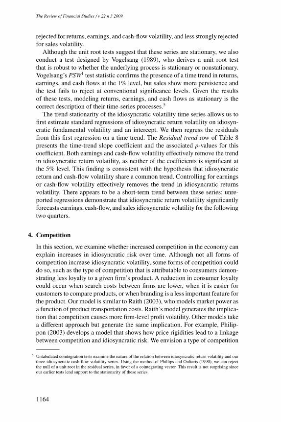
rejected for returns, earnings, and cash-flow volatility, and less strongly rejectedfor sales volatility.

Although the unit root tests suggest that these series are stationary, we alsoconduct a test designed by Vogelsang (1989), who derives a unit root testthat is robust to whether the underlying process is stationary or nonstationary.Vogelsang’s PSW1 test statistic confirms the presence of a time trend in returns,earnings, and cash flows at the 1% level, but sales show more persistence andthe test fails to reject at conventional significance levels. Given the resultsof these tests, modeling returns, earnings, and cash flows as stationary is thecorrect description of their time-series processes.5

The trend stationarity of the idiosyncratic volatility time series allows us tofirst estimate standard regressions of idiosyncratic return volatility on idiosyn-cratic fundamental volatility and an intercept. We then regress the residualsfrom this first regression on a time trend. The Residual trend row of Table 8presents the time-trend slope coefficient and the associated p-values for thiscoefficient. Both earnings and cash-flow volatility effectively remove the trendin idiosyncratic return volatility, as neither of the coefficients is significant atthe 5% level. This finding is consistent with the hypothesis that idiosyncraticreturn and cash-flow volatility share a common trend. Controlling for earningsor cash-flow volatility effectively removes the trend in idiosyncratic returnsvolatility. There appears to be a short-term trend between these series; unre-ported regressions demonstrate that idiosyncratic return volatility significantlyforecasts earnings, cash-flow, and sales idiosyncratic volatility for the followingtwo quarters.

4. Competition

In this section, we examine whether increased competition in the economy canexplain increases in idiosyncratic risk over time. Although not all forms ofcompetition increase idiosyncratic volatility, some forms of competition coulddo so, such as the type of competition that is attributable to consumers demon-strating less loyalty to a given firm’s product. A reduction in consumer loyaltycould occur when search costs between firms are lower, when it is easier forcustomers to compare products, or when branding is a less important feature forthe product. Our model is similar to Raith (2003), who models market power asa function of product transportation costs. Raith’s model generates the implica-tion that competition causes more firm-level profit volatility. Other models takea different approach but generate the same implication. For example, Philip-pon (2003) develops a model that shows how price rigidities lead to a linkagebetween competition and idiosyncratic risk. We envision a type of competition

5 Untabulated cointegration tests examine the nature of the relation between idiosyncratic return volatility and ourthree idiosyncratic cash-flow volatility series. Using the method of Phillips and Ouliaris (1990), we can rejectthe null of a unit root in the residual series, in favor of a cointegrating vector. This result is not surprising sinceour earlier tests lend support to the stationarity of these series.

1164


in which consumers shift their demand between firms within an industry, asopposed to changing their total demand for the industry’s product.6 When aparticular consumer ceases to purchase the product from one firm and initiatesa relationship with a second firm, the first firm loses product to the benefit ofthe second firm, inducing a lower correlation between the firms’ cash flows,and therefore, more idiosyncratic risk. Some examples of this type of competi-tion include charge card solicitations that entice a consumer to transfer balancesfrom a competitor, long-distance carrier promotions that pay customers to leavea competitor, and search engines that enable Internet consumers to compareprices from several vendors.

4.1 Analytical exampleThe impact of easier substitution between products can be illustrated with anexample. Consider a two-firm industry in which the firms have the followingcost functions:

C1 = w1

2q2

1 (10)

and

C2 = w2

2q2

2 . (11)

The parameters w1 and w2 can be considered as either input costs or atechnological parameter that affects productivity. We assume that the w’s arestochastic and thus a source of volatility shocks to the production process. Theprices of the two firms’ products are denoted by

p1 = θ − q1 − kq2 (12)

and

p2 = θ − q2 − kq1, (13)

where θ is an industry demand shock that is common to both firms, and k is aparameter assumed to lie between zero and unity that is related to how closelyconsumers view the two products as substitutes. When k = 0, no substitutionoccurs and both firms produce as monopolists. For positive k, each firm’sproduction decision is determined by a Cournot equilibrium, in which eachfirm solves for optimal production treating the other firm’s production decisionas given. For the case of k = 1, the standard case of Cournot competitionmaintains.

6 One example is provided by Agarwal, Baranth, and Viswanathan (2004), who document a link between eCom-merce adoption and volatility, which they attribute to increased demand uncertainty as well as product marketcompetition following eCommerce adoption.

1165


We assume that both firms observe the shocks to θ, w1, and w2 at the beginningof each period, and choose optimal production within the time period based onthis knowledge.

We can write firm 1’s profit function as

π1 = (θ − q1 − kq2) q1 − w1

2q2

1 . (14)

The first-order condition to maximize profit can be written as

0 = θ − kq2 − q1 (2 + w1) . (15)

Solving for q1,

q1 = θ − kq2

2 + w1. (16)

Appealing to the definition of Cournot equilibrium and to the fact that thefirms are isomorphic, the optimal quantities are given by

q1 = θ (2 + w2 − k)

(2 + w1) (2 + w2) − k(17)

and

q2 = θ (2 + w1 − k)

(2 + w1) (2 + w2) − k. (18)

Substituting (17) and (18) into (14) yields the optimal profit for firm 1,

π1 = θ2 (2 + w2 − k) (2k2 + (2 + w1) (2 + w2) − k (4 + w1))

2 (k − (2 + w1) (2 + w2))2 .

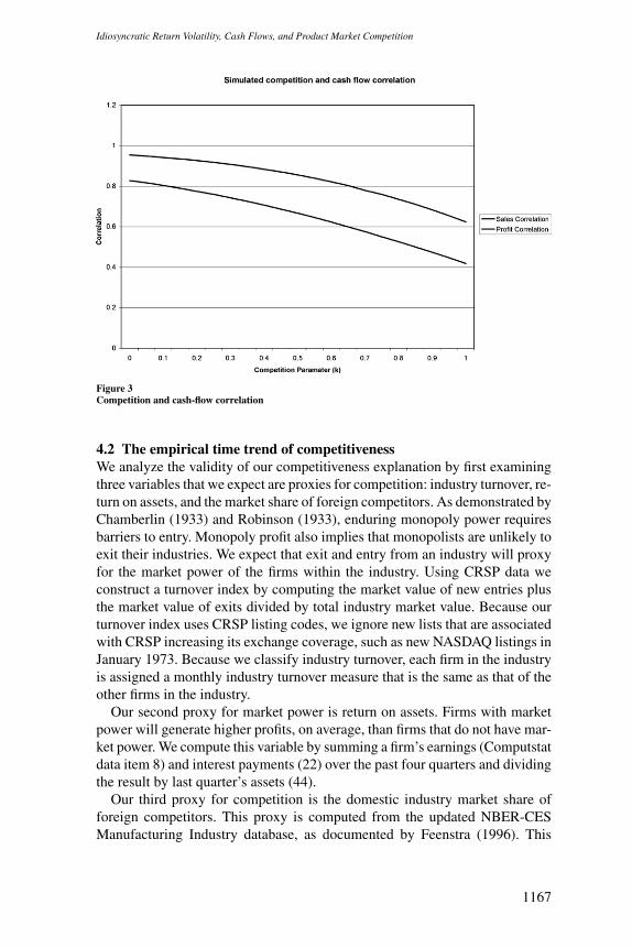
The analogous formula can be solved for firm 2’s profit. From these equationswe investigate the impact of shocks to θ, w1, and w2 on the correlation betweenthe firms’ profits. Specifically, we assume that θ can be 0.8, 1.0, or 1.2, each withprobability 1/3, and w1 and w2 can be 0.5, 1.0, or 1.5, again each with probability1/3. We assume that all three shocks are independent. This framework creates27 (3 × 3 × 3) distinct states, each with equal probability. For each individualstate we compute both firms’ profits. Using the production and profit outcomefrom all possible states, we compute the correlation between profits.

Figure 3 graphs the relation between the competition parameter k and thecorrelation between the two firms’ profits and sales. The source of positivecorrelation between firms comes from the industry-wide shocks θ, whereasthe negative correlation is induced from the input price shocks w1 and w2. Asthe industry becomes more competitive (k increases), both correlations fall.

1166


Figure 3Competition and cash-flow correlation

4.2 The empirical time trend of competitivenessWe analyze the validity of our competitiveness explanation by first examiningthree variables that we expect are proxies for competition: industry turnover, re-turn on assets, and the market share of foreign competitors. As demonstrated byChamberlin (1933) and Robinson (1933), enduring monopoly power requiresbarriers to entry. Monopoly profit also implies that monopolists are unlikely toexit their industries. We expect that exit and entry from an industry will proxyfor the market power of the firms within the industry. Using CRSP data weconstruct a turnover index by computing the market value of new entries plusthe market value of exits divided by total industry market value. Because ourturnover index uses CRSP listing codes, we ignore new lists that are associatedwith CRSP increasing its exchange coverage, such as new NASDAQ listings inJanuary 1973. Because we classify industry turnover, each firm in the industryis assigned a monthly industry turnover measure that is the same as that of theother firms in the industry.

Our second proxy for market power is return on assets. Firms with marketpower will generate higher profits, on average, than firms that do not have mar-ket power. We compute this variable by summing a firm’s earnings (Computstatdata item 8) and interest payments (22) over the past four quarters and dividingthe result by last quarter’s assets (44).

Our third proxy for competition is the domestic industry market share offoreign competitors. This proxy is computed from the updated NBER-CESManufacturing Industry database, as documented by Feenstra (1996). This

1167


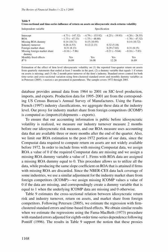
Table 9Cross-sectional and time-series influence of return on assets on idiosyncratic stock-returns volatility

Independent variable Specification

Intercept −4.73 (−147.32) −4.79 (−153.92) −4.25 (−19.93) −4.20 (−28.55)ROA −1.73 (−47.33) −1.75 (−48.80) −1.70 (−47.32)Missing ROA dummy 0.14 (10.71) 0.15 (10.95) 0.14 (10.72)Industry turnover 0.26 (4.53) 0.12 (2.13) 0.32 (5.18)Foreign market share 0.31 (8.13) 0.29 (7.02) 0.31 (8.15)Missing foreign market share

dummy−0.16 (−7.86) −0.21 (−9.64) −0.16 (−7.83)

Monthly fixed effects Yes Yes Yes YesR2% 16.89 16.08 12.28 16.89

Estimation of the effect of firm level idiosyncratic volatility on (1) the reported four-quarter return on assetsfrom quarterly statements that ended at least 3 months in the past; (2) a dummy variable that equals 1 if returnon assets is missing; and (3) the 2-month prior turnover of the firm’s industry. Standard errors control for bothtime-series and cross-sectional variation using firm-clustered standard errors and monthly dummy variables asin Petersen (2005). t-statistics are presented in parentheses. The sample covers 1972 through 2001.

database provides annual data from 1964 to 2001 on SIC-level production,imports, and exports. Production data for 1995–2001 are from the correspond-ing US Census Bureau’s Annual Survey of Manufactures. Using the Fama-French (1997) industry classifications, we aggregate these data at the industrylevel. Our proxy for industry market share from foreign competitors (ICOMP)is computed as (imports)/(shipments – exports).

To ensure that our accounting information is public before idiosyncraticvolatility is realized, we measure our industry turnover measure 2 monthsbefore our idiosyncratic risk measure, and our ROA measure uses accountingdata that are available three or more months after the end of the quarter. Also,we limit our ROA estimation to the post-1972 portion of our data, since theCompustat data required to compute return on assets are not widely availablebefore 1972. In order to include firms with missing Compustat data, we assignROA a value of 0 if the required Compustat data are missing and we assign amissing ROA dummy variable a value of 1. Firms with ROA data are assigneda missing ROA dummy equal to 0. This procedure allows us to utilize all thedata, while producing the same slope coefficient on ROA that is attained if firmswith missing ROA are discarded. Since the NBER-CES data lack coverage ofsome industries, we use a similar adjustment for the industry market share fromforeign competitors (ICOMP)—we assign missing ICOMP values a value of0 if the data are missing, and correspondingly create a dummy variable that isequal to 1 when the underlying ICOMP data are missing and 0 otherwise.

Table 9 estimates the cross-sectional relation between idiosyncratic returnrisk and industry turnover, return on assets, and market share from foreigncompetitors. Following Petersen (2005), we estimate the regression with firm-clustered standard errors and time-based fixed effects. We obtain similar resultswhen we estimate the regressions using the Fama-MacBeth (1973) procedurewith standard errors adjusted for eighth-order time-series dependence followingPontiff (1996). The results in Table 9 support the notion that these proxies

1168


for market power relate to idiosyncratic volatility. There is a strong negativerelation between ROA and future idiosyncratic volatility and there is a strongpositive relation between industry turnover and future idiosyncratic volatility.As predicted, there is a statistically significant positive relation between marketshare from foreign competitors and idiosyncratic return volatility. Our proxiesfor competition have a strong cross-sectional effect on idiosyncratic volatility.

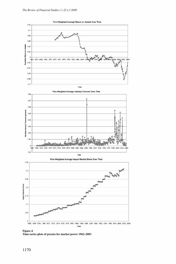
A time-series analysis is needed to ascertain whether our competition proxiessuggest a trend toward more competition. Unlike in the cross-sectional tests,we do not use a missing variable transformation, and thus our ROA and ICOMPvariables sometimes have missing data. Each data point represents an averageacross all firms with data. Since ICOMP and turnover are calculated at theindustry level, industries with larger numbers of firms will have a larger influ-ence on the time-series plot. Figure 4 examines the time-series properties ofthe cross-sectional averages of all three of our proxies. As the top plot demon-strates, there has been a trend toward lower ROA. In fact, since the late 1980s,the average ROA has tended to be negative, consistent with a trend toward moreaggressive competition. The second plot is consistent with increases in indus-try turnover, especially in the 1999–2002 period. The last plot demonstratesa notable increase in foreign competition. Over this time period, the typicaldomestic industry experienced a sevenfold increase in foreign market share.This plot is marked by substantial annual variation and minor monthly variationsince information on industry sales and import data is generated annually, yetthe monthly averages vary as the number of firms shifts within the year.

4.3 Evidence from deregulated industriesSeveral industry groups have experienced significant deregulation over the past40 years. Since deregulation reduces the barriers to entry that enable marketpower, we test for the impact of deregulation on idiosyncratic risk by exam-ining whether deregulated industries experience higher or lower than normalincreases in idiosyncratic volatility. We use the seven industries that Andrade,Mitchell, and Stafford (2001) list as having undergone a discrete deregulatoryexperience: airlines (deregulated in 1978), banks and thrifts (1994), entertain-ment (1984), natural gas (1978), telecommunications (1996), trucking (1980),and utilities (1992).

We form industries using an extension of the Fama-French (1997) 49 industrygroup classifications, in which we create new subindustries that correspond tothe Andrade, Mitchell, and Stafford (2001) deregulated industries. Specifically,we form an airline industry (AIR) from firms with SIC codes between 4500 and4599 that were previously included in the transportation industry (TRANS); anentertainment industry (ENTR) from firms with SIC codes between 7800 and7841 that were previously included in the broader Fama-French entertainmentindustry (FUN); a natural gas industry (NTGAS) from firms with SIC codesbetween 1310 and 1389 that were previously included in petroleum and naturalgas (ENRGY); a trucking industry from firms with SIC codes between 4210 and

1169


Figure 4Time-series plots of proxies for market power 1962–2003

1170


Table 10Idiosyncratic volatility and deregulation

Before deregulation After deregulation Difference

N Mean N Mean

Panel A: Log-relative idiosyncratic volatility of deregulated industries, where idiosyncratic risk is definedrelative to an equal-weighted market indexAir transport 156 0.001 324 −0.1338 −0.135Banks and thrifts 228 −1.182 252 −0.910 0.272Entertainment 228 0.429 252 0.561 0.132Natural gas 156 0.304 324 0.275 −0.029Telecommunications 372 −0.275 108 0.115 0.390Trucking 180 −0.344 300 −0.161 0.181Utilities 324 −1.292 156 −0.868 0.425Average difference t-test 0.177 (2.26)Panel B: Log-relative idiosyncratic volatility of deregulated industries, where idiosyncratic risk is definedrelative to an equal-weighted industry indexAir transport 156 −0.108 324 −0.161 −0.0532Banks and thrifts 228 −1.266 252 −0.918 0.349Entertainment 228 0.404 252 0.551 0.148Natural gas 156 0.309 324 0.266 −0.04Telecommunications 372 −0.276 108 0.119 0.395Trucking 180 −0.394 300 −0.183 0.211Utilities 324 −1.328 156 −0.880 0.448Average difference t-test 0.208 (2.71)

This table presents data on the magnitude of the log ratio of mean idiosyncratic volatility in deregulated industriesdivided by the magnitude of mean idiosyncratic volatility in the market. There are a total of 480 industry monthsin the sample from 1964 to 2003. The t-test presents a test of whether relative idiosyncratic volatility in thederegulated industry increases subsequent to the passage of the deregulation legislation.

4219 that were previously included in transportation (TRANS); and a bankingand thrift industry (B&THR) for firms with SIC codes between 6000 and 6036that were previously a subset of the Fama-French banking industry (BANKS).This produces a total of 53 industries.

We consider idiosyncratic risk measures relative to both the market and theparticular industry. As described in Section 1, market (industry) idiosyncraticrisk is calculated for each firm by computing the variance of the firm’s stockreturn less the return of the equal-weighted market (industry) index in a givenmonth. In order to control for marketwide trends in idiosyncratic risk, we dividethis measure by the average idiosyncratic risk of all firms in that month. Thisratio is transformed by the natural log operator and an industry average logratio is computed using all the firms in the industry.

Table 10 presents results using the log relative market (panel A) and log rel-ative industry (panel B) idiosyncratic risk measures. The results in both panelsare similar—five of seven industries experience increases in idiosyncratic riskafter deregulation. Since our risk variable is measured in logs, we can interpretthe difference as a percentage change in risk. The mean change for the log rel-ative market (industry) idiosyncratic risk is 17.7% (20.8%) after deregulation,statistically significant at the 5% (1%) level. These results are consistent withdecreases in market power coinciding with increases in idiosyncratic risk.

1171


4.4 Evidence from international competitionThe previous section argues that more competitive industries (deregulated in-dustries) have higher idiosyncratic volatility. This section examines whetherour cross-sectional conclusion on competitiveness and idiosyncratic volatilitycan be expanded across countries: do countries whose market environments aremore competitive have higher idiosyncratic volatility?

We obtain data on idiosyncratic volatility trends for the G-7 countries fromGuo and Savickas (2004). Competitiveness data come from the World Eco-nomic Forum. Each year the World Economic Forum produces the GlobalCompetitiveness Index (GCI), which is a rank of country competitiveness. TheGCI has an advantage relative to a single-industry deregulation event in thatit is extremely broad; it incorporates a great number of factors that can affectthe competitive environment in a particular country (Blanke, Paua, and Sala-I-Martin, 2004). The index is disaggregated into three components: technology(50%), public institutions (25%), and macroeconomic environment (25%).

The Guo and Savickas data begin in 1962 for the United States, 1965 forthe United Kingdom, and 1973 for all other G-7 countries, and end in 2003.From World Economic Forum published documents we obtain overall countrycompetitiveness ranks for 2003. Our competitiveness explanation implies thatboth positive changes in competitiveness and positive changes in technologywill be associated with positive changes in idiosyncratic risk. A direct test ofeconomy-wide competitiveness changes is not possible as the GCI index didnot exist for much of the Guo and Savickas sample period. Rather, we use the2003 GCI rank as a proxy for the change in economy-wide competitiveness overtime. This substitution induces an errors-in-variables problem, which will biasour test statistic toward the null. However, we can directly test our explanationby obtaining data on the change in rank (1973–2003) of a key component ofthe GCI technology subindex: US patents per capita. While patents per capitarepresent only part of the GCI, the data are available back to 1973, the firstyear all G-7 countries had returns data. Thus, the patent data can be usedto determine whether changes over time in technological competitiveness arecorrelated with changes over time in idiosyncratic volatility.

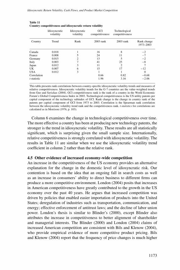
The CI ranks the most competitive environment as 1, and all other countriesthat are less competitive have higher ranks. Table 11 presents the trend inidiosyncratic volatility for G-7 countries in column 2 and the rank of volatilitygrowth for each country in column 3. Column 4 presents the 2003 overallcountry competitiveness rank. Column 5 presents the 2003 patents per capita(technological competitiveness) rank, and column 6 presents the change intechnological competitiveness from 1973 to 2003.

Spearman’s rank correlations between idiosyncratic volatility and competi-tiveness are presented at the bottom of columns 4, 5, and 6. The large positivecorrelations between volatility growth and both the 2003 competitiveness rankand the technology rank indicate that more competitive economies have expe-rienced greater increases in idiosyncratic risk.

1172


Table 11Country competitiveness and idiosyncratic return volatility

Idiosyncraticvolatility

Idiosyncraticvolatility

GCIcompetitiveness

Technologicalcompetitiveness

Country Trend Rank 2003 rank 2003 rank Rank change1973–2003

Canada 0.018 1 16 8 −2France 0.008 5 24 11 −7Germany 0.015 2 13 5 −2Italy 0.003 7 41 25 −8Japan 0.012 3 11 2 7UK 0.007 6 15 17 −12USA 0.012 3 1 1 0Correlation 0.66 0.82 −0.68t-statistic 1.96 3.16 −2.06

This table presents rank correlations between country-specific idiosyncratic volatility trends and measures ofrelative competitiveness. Idiosyncratic volatility trends for the G-7 countries are the value-weighted trendsfrom Guo and Savickas (2004). GCI competitiveness rank is the rank of a country in the World EconomicForum’s Global Competitiveness Index in 2003. Technological competitiveness is the US utility patents percapital component of the technology subindex of GCI. Rank change is the change in country rank of thepatents per capital component of GCI from 1973 to 2003. Correlation is the Spearman rank correlationbetween the idiosyncratic volatility trend rank and the competitiveness rank. t-statistics for correlations arecalculated as in Morrison (1976, p. 103).

Column 6 examines the change in technological competitiveness over time.The more effective a country has been at producing new technology patents, thestronger is the trend in idiosyncratic volatility. These results are all statisticallysignificant, which is surprising given the small sample size. Internationally,relative competitiveness is strongly correlated with idiosyncratic volatility. Theresults in Table 11 are similar when we use the idiosyncratic volatility trendcoefficient in column 2 rather than the relative rank.

4.5 Other evidence of increased economy-wide competitionAn increase in the competitiveness of the US economy provides an alternativeexplanation for the change in the domestic level of idiosyncratic risk. Ourcontention is based on the idea that an ongoing fall in search costs as wellas an increase in consumers’ ability to direct business to different firms canproduce a more competitive environment. London (2004) posits that increasesin American competitiveness have greatly contributed to the growth in the USeconomy over the past 40 years. He argues that increased competition wasdriven by policies that enabled easier importation of products into the UnitedStates; deregulation of industries such as transportation, communication, andenergy; effective enforcement of antitrust laws; and the decline of labor unionpower. London’s thesis is similar to Blinder’s (2000), except Blinder alsoattributes the increase in competitiveness to better alignment of shareholderand managerial interests. The Blinder (2000) and London (2004) claims ofincreased American competition are consistent with Bils and Klenow (2004),who provide empirical evidence of more competitive product pricing. Bilsand Klenow (2004) report that the frequency of price changes is much higher

1173


in the mid-1990s than that in earlier published reports. Logically linked tocompetitiveness, price changes were most frequent for consumer nondurablesand products that experienced higher introduction of substitutes, consistent withgreater consumer choice in the recent economy. Chun et al. (2004) generallyconcur with our arguments and contend that the rapid diffusion of informationtechnology plays a major role in the acceleration of Schumpeter’s (1942) forcesof creative destruction in the economy and the resulting increase in firm-levelvolatility.

4.6 The competitiveness explanation and other studiesThe idiosyncratic risk literature has examined two broad areas: cross-sectionaland time-series differences in idiosyncratic risk in the US markets, and cross-sectional differences among idiosyncratic risk levels in foreign markets. Thecompetitiveness explanation, along with our findings of increases in funda-mental idiosyncratic volatility, provides a new interpretation of these streamsof literature.

Papers in the first stream of the literature have attributed the rise in idiosyn-cratic return volatility to other variables. For example, Brown and Kapadia(2007) show that initial public offerings have resulted in the listing of morevolatile firms on exchanges. They argue that this trend explains much of thetrend in idiosyncratic volatility. Bennett and Sias (2006) relate the increase inidiosyncratic volatility to the increased presence of small stocks. Our resultsshow that these explanations only explain about 1/3 of the time trend of fun-damental volatility, whereas competitiveness provides an explanation that cancoexist with these studies and can explain the remaining increase.

The second stream of idiosyncratic risk literature investigates differencesin cross-country levels of R2s. These papers commonly attribute idiosyncraticrisk levels to the efficiency of financial markets. Morck, Yeung, and Yu (2000)show that systematic risk and price synchronicity are higher in countries withpoor corporate governance, even after controlling for obvious cross-countrydifferences in industrial structure and economic activity. They argue that theirfindings are consistent with strong investor protection. Specifically, sophisti-cated investors have a lower incentive to impute firm-specific information instock prices through their trading when investor protection is weak. Jin andMyers (2006) extend the Morck et al. (2000) argument by considering theeffects of opacity on the relation between country-specific R2s and corporategovernance. They maintain that opacity is required to confirm the Morck et al.(2000) results because more opaque environments, combined with poor cor-porate governance, enable insiders to capture a larger proportion of the firm’soperating cash flows. This leads to lower firm-specific risk for investors andhigher country R2s.

These papers provide tenable arguments for cross-sectional differences in theimportance of idiosyncratic volatility in a particular country’s market. Cross-sectional differences in legal environments can be obvious and noticeable,

1174


and they should have important effects. However, there are problems applyingsome of these ideas to the time-series trend in domestic idiosyncratic volatility,particularly in the past 20 years when the growth of idiosyncratic volatilityhas accelerated. It is doubtful that legal protection provided to investors in theUnited States has changed significantly in the past 20 years. We argue thatdomestic changes in the above set of cross-sectional explanations are unlikelyto be sufficient, by themselves, to explain the increase in idiosyncratic volatilityin the United States.

Carlin (2006) shows that firms can use opaqueness to create a less com-petitive product market. Countries with better information environments andbetter legal systems will have greater transparency, which makes it more dif-ficult for firms to protect monopoly profits. Our exploratory findings in Table11 lend support to the idea that competition is related to cross-country differ-ences in idiosyncratic risk. Both the competitiveness explanation and Morcket al.’s (2000) trading-information hypothesis predict a relation between marketopaqueness and idiosyncratic volatility. Competition is a broader explanationof cross-country differences in R2s than the trading information explanation,since it is also consistent with differences in fundamental idiosyncratic risk.

5. Conclusion

This paper documents a significant increase over time in the idiosyncraticvolatility of firm-level earnings, cash flows, and sales. Over the period 1964–2003, the magnitude of the increase in the idiosyncratic volatility of earnings,cash flows, and sales is large enough to explain why a rational stock market’sidiosyncratic stock-return volatility has increased dramatically over the sameperiod. We rule out the possibility that this finding is explained entirely by newlistings, data provider coverage, higher proportions of smaller firms, changes inthe composition of industries, or a general trend among firms toward focusingon fewer lines of business.

We explore the possibility that increased competition is the source of theincrease in idiosyncratic volatility. We construct proxies for competition andconduct both cross-sectional and time-series tests. In support of our explana-tion, we find that return on assets, which is negatively related to idiosyncraticvolatility in the cross-section, has declined over our sample period. Industryturnover, defined as the proportion of industry market value that enters and exitsan industry in a given time period, is positively related to future idiosyncraticvolatility. Further, the overall market has demonstrated an increase in industryturnover. We find a similar pattern in the market shares of foreign competitors.Cross-sectionally, firms in industries with more foreign competition experiencemore idiosyncratic risk, and time-series plots show that the level of foreign com-petition faced by the typical domestic firm has dramatically increased. Finally,since deregulation is associated with increased competition, we examine in-dustries that have undergone significant deregulation. We find that deregulation

1175


is associated with significant increases in idiosyncratic volatility, even beyondthe general time trend that we document. Examining cross-country trends inidiosyncratic volatility, we show that countries with greater growth in idiosyn-cratic stock-return volatility tend to have more competitive economies andundergo faster change in technological innovation. This mosaic of evidencelends support to the notion that economy-wide competition plays a role in therecent trend toward higher levels of idiosyncratic stock-return risk.

ReferencesAgarwal, D., S. Baranth, and S. Viswanathan. 2004. Technological Change and Stock Return Volatility: Evidencefrom eCommerce Adoptions. Working Paper, University of Maryland.

Andrade, G., M. Mitchell, and E. Stafford. 2001. New Evidence and Perspectives on Mergers. Journal ofEconomic Literature 15:103–20.

Bennett, J., R. Sias, and L. Starks. 2003. Greener Pastures and the Impact of Dynamic Institutional Preferences.The Review of Financial Studies 16:1203–38.

Bennett, J., and R. Sias. 2006. Why Company-Specific Risk Changes over Time. Financial Analysts Journal62:89–100.

Berger, P., and R. Hann. 2003. The Impact of SFAS No. 131 on Information and Monitoring. Journal ofAccounting Research 41:1–61.

Bils, M., and P. Klenow. 2004. The Importance of Sticky Prices. Journal of Political Economy 112:947–85.

Blanke, J., F. Paua, and X. Sala-I-Martin. 2004. The Growth Competitiveness Index: Analyzing Key Componentsof Sustained Economic Growth. World Economic Forum and Columbia University.

Blinder, A. 2000. How the Economy Came to Resemble the Model. Business Economics 1:16–25.

Brandt, M. W., A. Brav, and J. Graham. 2005. The Idiosyncratic Volatility Puzzle: Time Trend or SpeculativeEpisodes. Working Paper, Duke University.

Brown, G., and N. Kapadia. 2007. Firm-Specific Risk and Equity Market Development. Working Paper, Universityof North Carolina.

Brown, L. 1993. Earnings Forecasting Research: Its Implications for Capital Markets Research. InternationalJournal of Forecasting 9:295–320.

Brown, L., and J. Rozeff. 1979. Univariate Time-Series Models of Earnings per Share: A Proposed Model.Journal of Accounting Research 17:179–89.

Campbell, J., M. Lettau, B. Malkiel, and Y. Xu. 2001. Have Individual Stock Returns Become More Volatile?An Empirical Exploration of Idiosyncratic Risk. Journal of Finance 56:1–43.

Carlin, B. 2006. Strategic Price Complexity in Retail Financial Markets. Working Paper, Duke University.

Chamberlin, E. H. 1933. Theory of Monopolistic Competition. Cambridge, MA: Harvard University Press.

Chordia, T., R. Roll, and A. Subrahmanyam. 2001. Market Liquidity and Trading Activity. Journal of Finance56:501–30.

Chun, H., J. Kim, J. Lee, and R. Morck. 2004. Patterns of Co-Movement: The Role of Information Technologyin the U.S. Economy. Working Paper, University of Alberta.

Comin, D., and T. Philippon. 2005. The Rise in Firm-Level Volatility: Causes and Consequences, in M. Gertlerand K. Rogoff (eds.), NBER Macroeconomics Annual 2005, vol. 20, MIT Press, Cambridge, MA. USA 02142.

Dennis, P., and D. Strickland. 2004. The Determinants of Idiosyncratic Volatility. Working Paper, University ofVirginia and University of North Carolina.

1176


Fama, E., and K. French. 1997. Industry Costs of Equity. Journal of Financial Economics 43:153–93.

Fama, E., and J. MacBeth. 1973. Risk, Return, and Equilibrium: Empirical Tests. Journal of Political Economy81:607–36.

Feenstra, R. C. 1996. U.S. Imports, 1972–1994: Data and Concordances. Working Paper Series, NBER.

Guo, H., and R. Savickas. 2004. Aggregate Idiosyncratic Volatility in G7 Countries. Working Paper, FederalReserve Bank of St Louis and George Washington University.

Jin, L., and S. Myers. 2006. R2 around the World: New Theory and New Tests. Journal of Financial Economics76:257–92.

London, P. A. 2004. Competition Solution. Washington, DC: AEI Press.

Malkiel, B., and Y. Xu. 2003. Investigating the Behavior of Idiosyncratic Volatility. Journal of Business 76:613–44.

Morck, R., B. Yeung, and W Yu. 2000. The Information Content of Stock Markets: Why Do Emerging MarketsHave Synchronous Stock Price Movements? Journal of Financial Economics 58:215–60.

Morrison, D. F. 1976. Multivariate Statistical Methods, New York: McGraw-Hill.

Petersen, M. 2005. Estimating Standard Errors in Finance Panel Data Sets: Comparing Approaches. WorkingPaper, Northwestern University.

Philippon, T. 2003. An Explanation for the Joint Evolution of Firm and Aggregate Volatility. Working Paper,New York University.

Phillips, P. C., and S. Ouliaris. 1990. Asymptotic Properties of Residual Based Tests for Co-Integration. Econo-metrica 58:165–93.

Pontiff, J. 1996. Costly Arbitrage: Evidence from Closed-End Funds. Quarterly Journal of Economics 111:1135–51.

Raith, Michael. 2003. Competition, Risk and Managerial Incentives. American Economic Review 93:1425–36.

Robinson, J. 1933. Economics of Imperfect Competition. London: Macmillan.

Roll, R. 1988. R2. Journal of Finance 43:541–66.

Schumpeter, J. 1942. Capitalism, Socialism and Democracy. New York: Harper.

Schwert, W., and P. Seguin. 1990. Heteroskedasticity in Stock Returns. Journal of Finance 45:1129–55.

Sharpe, W. 1964. Capital Asset Prices: A Theory of Market Equilibrium under Conditions of Risk. Journal ofFinance 19:425–42.

Vogelsang, T. 1989. Trend Function Hypothesis Testing in the Presence of Serial Correlation. Econometrica66:123–48.

United States Census Bureau. 1996–2002. Annual Survey of Manufactures: Statistics for Industry Groups andIndustries, 1995–2001.

Wei, S., and C. Zhang. 2006. Why Did Individual Stocks Become More Volatile? Journal of Business 76:259–92.

1177

Documents

Idiosyncratic Return Volatility, Cash Flows, and Product ... · Idiosyncratic Return Volatility, Cash Flows, and Product Market Competition The paper is organized as follows. Section