Identifying Causal Effects in Time Series Models

Aaron Smith

UC Davis

July 27, 2015

Slides and references will be posted on my websitehttp://asmith.ucdavis.edu

1

Identifying Causal Effects in Time Series ModelsIf all the “Metrics” I Understand is in Mostly

Harmless Econometrics, How Should I Think AboutTime Series Analysis?

Aaron Smith

UC Davis

July 27, 2015

Slides and references will be posted on my websitehttp://asmith.ucdavis.edu

2

Outline

1. Potential Outcomes and Ideal ExperimentsI Internal validity vs external validity

I Single discrete events

I Multiple discrete events

2. Potential events every time periodI Everything is autocorrelated and everything is endogenous

I The impulse response as an average treatment effect

I Identification

3. Conclusion

3

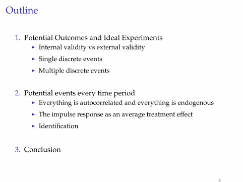
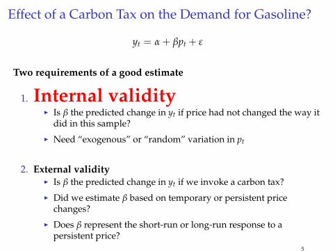
Effect of a Carbon Tax on the Demand for Gasoline?

yt = α + βpt + ε

Two requirements of a good estimate

1. Internal validityI Is β the predicted change in yt if price had not changed the way it

did in this sample?

I Need “exogenous” or “random” variation in pt

2. External validityI Is β the predicted change in yt if we invoke a carbon tax?

I Did we estimate β based on temporary or persistent pricechanges?

I Does β represent the short-run or long-run response to apersistent price?

4

Effect of a Carbon Tax on the Demand for Gasoline?

yt = α + βpt + ε

Two requirements of a good estimate

1. Internal validityI Is β the predicted change in yt if price had not changed the way it

did in this sample?

I Need “exogenous” or “random” variation in pt

2. External validityI Is β the predicted change in yt if we invoke a carbon tax?

I Did we estimate β based on temporary or persistent pricechanges?

I Does β represent the short-run or long-run response to apersistent price?

5

Case 1: Single Discrete Event

yt(Dt) =

yt(0) if Dt = 0 (untreated)

yt(1) if Dt = 1 (treated)

I Dt is the treatment variable

I Observation t has two potential outcomes depending onwhether the treatment is on or off.

I Average treatment effect is

ATE = E [yt(1)− yt(0)]

6

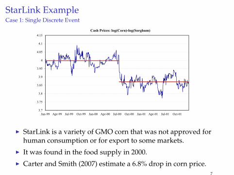
StarLink ExampleCase 1: Single Discrete Event

3.7

3.75

3.8

3.85

3.9

3.95

4

4.05

4.1

4.15

Jan-99 Apr-99 Jul-99 Oct-99 Jan-00 Apr-00 Jul-00 Oct-00 Jan-01 Apr-01 Jul-01 Oct-01

Cash Prices: log(Corn)-log(Sorghum)

I StarLink is a variety of GMO corn that was not approved forhuman consumption or for export to some markets.

I It was found in the food supply in 2000.

I Carter and Smith (2007) estimate a 6.8% drop in corn price.7

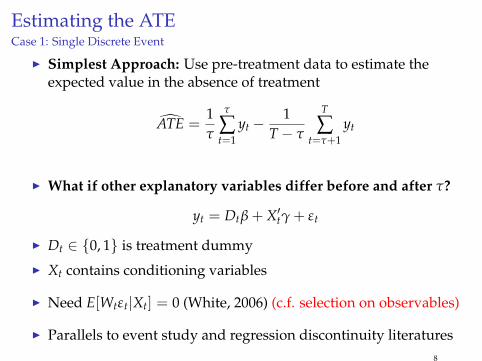
Estimating the ATECase 1: Single Discrete Event

I Simplest Approach: Use pre-treatment data to estimate theexpected value in the absence of treatment

ATE =1τ

τ

∑t=1

yt −1

T− τ

T

∑t=τ+1

yt

I What if other explanatory variables differ before and after τ?

yt = Dtβ + X′tγ + εt

I Dt ∈ 0, 1 is treatment dummy

I Xt contains conditioning variables

I Need E[Wtεt|Xt] = 0 (White, 2006) (c.f. selection on observables)

I Parallels to event study and regression discontinuity literatures8

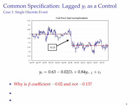
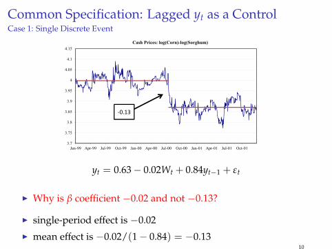
Common Specification: Lagged yt as a ControlCase 1: Single Discrete Event

3.7

3.75

3.8

3.85

3.9

3.95

4

4.05

4.1

4.15

Jan-99 Apr-99 Jul-99 Oct-99 Jan-00 Apr-00 Jul-00 Oct-00 Jan-01 Apr-01 Jul-01 Oct-01

Cash Prices: log(Corn)-log(Sorghum)

‐0.13

yt = 0.63− 0.02Dt + 0.84yt−1 + εt

I Why is β coefficient −0.02 and not −0.13?

I

I9

Common Specification: Lagged yt as a ControlCase 1: Single Discrete Event

3.7

3.75

3.8

3.85

3.9

3.95

4

4.05

4.1

4.15

Jan-99 Apr-99 Jul-99 Oct-99 Jan-00 Apr-00 Jul-00 Oct-00 Jan-01 Apr-01 Jul-01 Oct-01

Cash Prices: log(Corn)-log(Sorghum)

‐0.13

yt = 0.63− 0.02Wt + 0.84yt−1 + εt

I Why is β coefficient −0.02 and not −0.13?

I single-period effect is −0.02

I mean effect is −0.02/(1− 0.84) = −0.1310

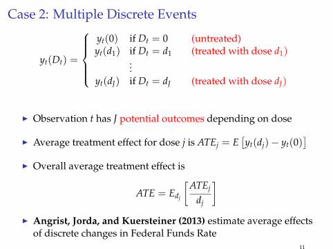
Case 2: Multiple Discrete Events

yt(Dt) =

yt(0) if Dt = 0 (untreated)yt(d1) if Dt = d1 (treated with dose d1)

...yt(dJ) if Dt = dJ (treated with dose dJ)

I Observation t has J potential outcomes depending on dose

I Average treatment effect for dose j is ATEj = E[yt(dj)− yt(0)

]I Overall average treatment effect is

ATE = Edj

[ATEj

dj

]I Angrist, Jorda, and Kuersteiner (2013) estimate average effects

of discrete changes in Federal Funds Rate11

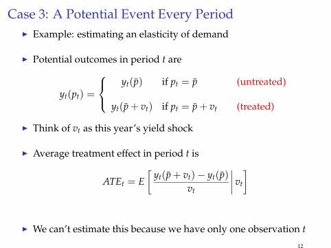
Case 3: A Potential Event Every PeriodI Example: estimating an elasticity of demand

I Potential outcomes in period t are

yt(pt) =

yt(p) if pt = p (untreated)

yt(p + vt) if pt = p + vt (treated)

I Think of vt as this year’s yield shock

I Average treatment effect in period t is

ATEt = E[

yt(p + vt)− yt(p)vt

∣∣∣∣ vt

]

I We can’t estimate this because we have only one observation t

12

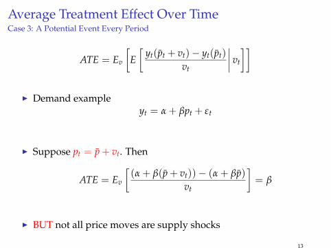
Average Treatment Effect Over TimeCase 3: A Potential Event Every Period

ATE = Ev

[E[

yt(pt + vt)− yt(pt)

vt

∣∣∣∣ vt

]]

I Demand exampleyt = α + βpt + εt

I Suppose pt = p + vt. Then

ATE = Ev

[(α + β(p + vt))− (α + βp)

vt

]= β

I BUT not all price moves are supply shocks

13

EndogeneityCase 3: A Potential Event Every Period

I Demand example

yt = α + βpt + εt

pt = p + vt + γεt

I Could use an instrumental variable zt with the properties

E[ztεt] = 0 and E[ztvt] 6= 0

I BUT instrument typically has persistent effect on vtI zt, zt−1, zt−2, ... all affect vt

I e.g., poor growing-season weather this year may affect prices for afew years

I AND instrument may be autocorrelatedI We aren’t getting a new, clean experiment every period

14

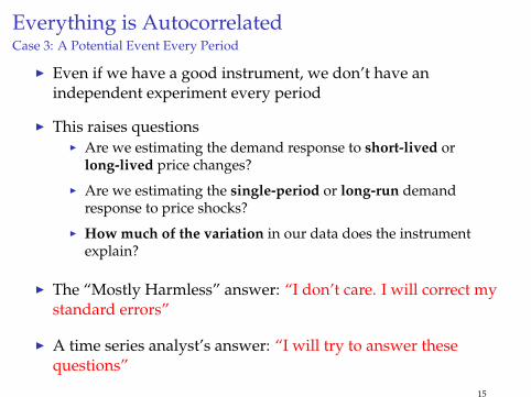
Everything is AutocorrelatedCase 3: A Potential Event Every Period

I Even if we have a good instrument, we don’t have anindependent experiment every period

I This raises questionsI Are we estimating the demand response to short-lived or

long-lived price changes?

I Are we estimating the single-period or long-run demandresponse to price shocks?

I How much of the variation in our data does the instrumentexplain?

I The “Mostly Harmless” answer: “I don’t care. I will correct mystandard errors”

I A time series analyst’s answer: “I will try to answer thesequestions”

15

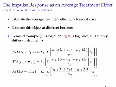
The Impulse Response as an Average Treatment EffectCase 3: A Potential Event Every Period

I Estimate the average treatment effect of a forecast error

I Estimate this object at different horizons

I Demand example (qt is log quantity, pt is log price, zt is supplyshifter (instrument))

ATE(zt zt+k) = Ev

[E[

zt+k(zt + vzt)− zt+k(zt)

vzt

∣∣∣∣ vzt

]]ATE(zt pt+k) = Ev

[E[

pt+k(zt + vzt)− pt+k(zt)

vzt

∣∣∣∣ vzt

]]ATE(zt yt+k) = Ev

[E[

yt+k(zt + vzt)− yt+k(zt)

vzt

∣∣∣∣ vzt

]]

16

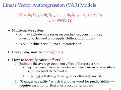
Linear Vector Autoregression (VAR) Models

Xt = Φ1Xt−1 + Φ2Xt−2 + ... + ΦpXt−p + c0 + c1t + εt

εt ∼ WN(0, Ω)

I Multivariate systemI Xt may include time series on production, consumption,

inventory, demand and supply shifters, and futuresI WN ≡ “white noise” ≡ no autocorrelation

I Everything may be endogenous

I How to identify causal effects?1. Estimate the average treatment effect of forecast errors

I requires assumptions on meaning of contemporaeous correlations,i.e., off-diagonal elements of Ω

I If E[ε1tε2t] 6= 0, did ε1t cause ε2t or the other way around?

2. “Granger causality,” which is another word for predictability —requires assumption that effects occur after causes

17

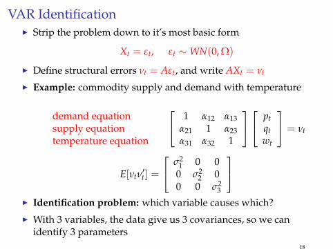
VAR IdentificationI Strip the problem down to it’s most basic form

Xt = εt, εt ∼ WN(0, Ω)

I Define structural errors νt = Aεt, and write AXt = νt

I Example: commodity supply and demand with temperature

demand equationsupply equationtemperature equation

1 α12 α13α21 1 α23α31 α32 1

ptqtwt

= νt

E[νtν′t ] =

σ21 0 0

0 σ22 0

0 0 σ23

I Identification problem: which variable causes which?

I With 3 variables, the data give us 3 covariances, so we canidentify 3 parameters

18

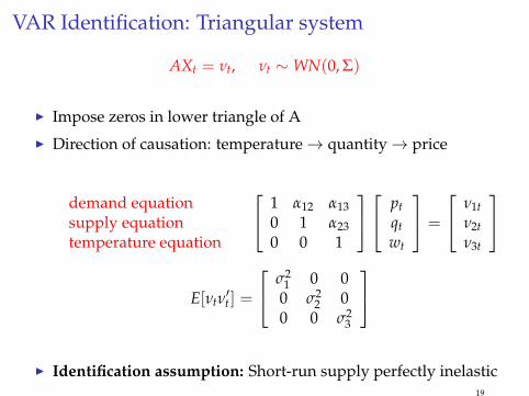
VAR Identification: Triangular system

AXt = νt, νt ∼ WN(0, Σ)

I Impose zeros in lower triangle of A

I Direction of causation: temperature→ quantity→ price

demand equationsupply equationtemperature equation

1 α12 α130 1 α230 0 1

ptqtwt

=

ν1tν2tν3t

E[νtν′t ] =

σ21 0 0

0 σ22 0

0 0 σ23

I Identification assumption: Short-run supply perfectly inelastic19

VAR Identification: Known Supply Elasticity

AXt = νt, νt ∼ WN(0, Σ)

I Impose a known value in A

I Could also get partial identification by specifying a range for α21

demand equationsupply equationtemperature equation

1 α12 α130.1 1 α230 0 1

ptqtwt

= νt

E[νtν′t ] =

σ21 0 0

0 σ22 0

0 0 σ23

I Identification assumption: Short-run supply elasticity equals 0.120

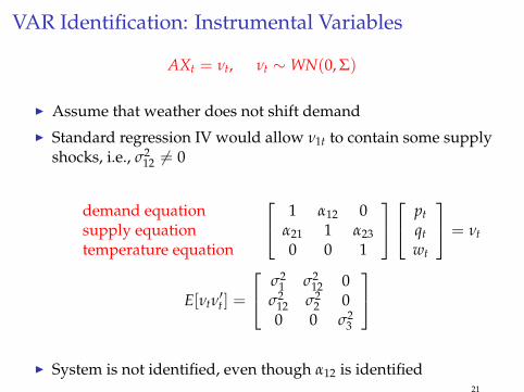
VAR Identification: Instrumental Variables

AXt = νt, νt ∼ WN(0, Σ)

I Assume that weather does not shift demand

I Standard regression IV would allow ν1t to contain some supplyshocks, i.e., σ2

12 6= 0

demand equationsupply equationtemperature equation

1 α12 0α21 1 α230 0 1

ptqtwt

= νt

E[νtν′t ] =

σ21 σ2

12 0σ2

12 σ22 0

0 0 σ23

I System is not identified, even though α12 is identified

21

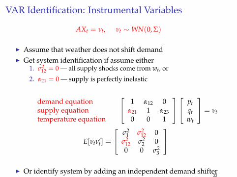
VAR Identification: Instrumental Variables

AXt = νt, νt ∼ WN(0, Σ)

I Assume that weather does not shift demandI Get system identification if assume either

1. σ212 = 0 — all supply shocks come from wt, or

2. α21 = 0 — supply is perfectly inelastic

demand equationsupply equationtemperature equation

1 α12 0α21 1 α230 0 1

ptqtwt

= νt

E[νtν′t ] =

σ21 σ2

12 0σ2

12 σ22 0

0 0 σ23

I Or identify system by adding an independent demand shifter

22

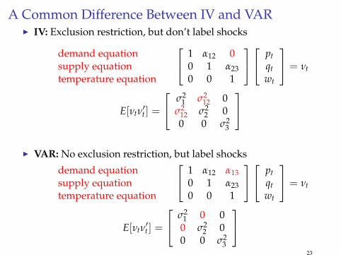
A Common Difference Between IV and VARI IV: Exclusion restriction, but don’t label shocks

demand equationsupply equationtemperature equation

1 α12 00 1 α230 0 1

ptqtwt

= νt

E[νtν′t ] =

σ21 σ2

12 0σ2

12 σ22 0

0 0 σ23

I VAR: No exclusion restriction, but label shocks

demand equationsupply equationtemperature equation

1 α12 α130 1 α230 0 1

ptqtwt

= νt

E[νtν′t ] =

σ21 0 0

0 σ22 0

0 0 σ23

23

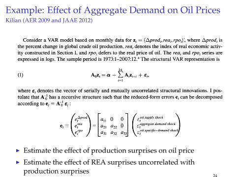
Example: Effect of Aggregate Demand on Oil PricesKilian (AER 2009 and JAAE 2012)

1058 THE AMERICAN ECONOMIC REVIEW JUNE 2009

strong demand for industrial commodities. Thus, one would want to be careful about associating the concurrent increases in the real price of oil with these events. This evidence underscores the

importance of disentangling the effects of demand shocks and supply shocks on the real price of oil.

II. Decomposing the Real Price of Oil

Numerous empirical and theoretical studies have investigated the response of macroeconomic

aggregates to changes in the price of oil. Implicit in this literature is the thought experiment that one can change the price of oil, while holding everything else constant, as would be the case if the price of oil were exogenous. To the extent that the price of oil is actually endogenous with

respect to the macroeconomic aggregates of interest, this thought experiment is violated. If there is no well defined cause, it becomes impossible to estimate its effect. This general principle has been recognized dating back to the Cowles Commission. As Thomas F. Cooley and Stephen F.

LeRoy (1985, 295) summarize, it is inadmissible to inquire about the effect of a change in one

endogenous variable on another, when the underlying experiment that led to the assumed varia tion in the endogenous variable is ambiguous.

This problem has not completely escaped attention. Implicitly or explicitly, many researchers have assumed that at least the major increases in the price of oil can be treated as exogenous. Recent research has demonstrated that this interpretation, which seemed reasonable at the time, does not hold up to scrutiny (see, e.g., Kilian 2008a). This means that without knowing what drove up the price of oil in the first place, it will be impossible to predict accurately the implica tions of higher oil prices. In this section, I present a methodology for decomposing unpredictable changes in the real price of oil into mutually orthogonal components with a structural economic

interpretation. This decomposition has immediate implications for how macroeconomists and

policymakers should think about oil price fluctuations.

A. The Structural VAR Model

Consider a VAR model based on monthly data for zt = (Aprodt,reat,rpot)', where Aprodt is the percent change in global crude oil production, reat denotes the index of real economic activ

ity constructed in Section I, and rpot defers to the real price of oil. The reat and rpot series are

expressed in logs. The sample period is 1973:1-2007:12.4 The structural VAR representation is

24

(1) A0z, = a + ? AiZt_i + et, i=i

where et denotes the vector of serially and mutually uncorrelated structural innovations. I pos tulate that A"0! has a recursive structure such that the reduced-form errors e, can be decomposed according to e,

= A~o et:

AA/^A ^^ q q I

eoil supply shock \

et=[er 1= a2l a22 0 I segregate demand shock

J \ r, rP? I n r, r, \ t~?M specific-demand shock! \et j ^a3l a32 a33j \et y

4 The starting date is dictated by the availability of the oil production data from the US Department of Energy. I

compute the log differences of world crude oil production in millions of barrels pumped per day (averaged by month). The real oil price series is obtained based on the refiner acquisition cost of imported crude oil, as provided by the US

Department of Energy since 1974:1 and extended backward as in Barsky and Kilian (2002). The nominal oil price has been deflated by the US CPI.

This content downloaded from 169.237.188.145 on Tue, 4 Feb 2014 13:04:27 PMAll use subject to JSTOR Terms and Conditions

I Estimate the effect of production surprises on oil price

I Estimate the effect of REA surprises uncorrelated withproduction surprises

24

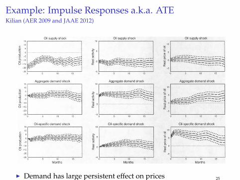
Example: Impulse Responses a.k.a. ATEKilian (AER 2009 and JAAE 2012)

VOL. 99 NO. 3 KILIAN: NOT ALL OIL PRICE SHOCKS AREALIKE 1061

Oil supply shock J -!-!-1-(-!-!

0.5 -

-1 I_I_i_I_I_l_i_ 1975 1980 1985 1990 1995 2000 2005

Aggregate demand shock 1 -(-!-(-(-(-]

-0.5 r

-1 I_I_I_I_I_I_I_I 1975 1980 1985 1990 1995 2000 2005

Oil-specific demand shock 1 -j-j-j-(-j-(

-1 I_I_I_I_I_I_I_ 1975 1980 1985 1990 1995 2000 2005

Figure 2. Historical Evolution of the Structural Shocks, 1975-2007

Note: Structural residuals implied by model (1), averaged to annual frequency.

Oil supply shock Oil supply shock Oil supply shock 15 I-i 10 i-1 1-1

10 10

3 o . f 5 * 5. g 5 #. s 8 .

-20*5*' ?-...---- i

_25 I-.-.-.-1 _5 I-.-,-.-1 1-.-1-1 0 5 10 15 0 5 10 15 0 5 10 15

Aggregate demand shock Aggregate demand shock Aggregate demand shock 15 i-1-1 10 i-1-1 I-1

10 _ _ 10

= S ?. . . . 5

? ? *-. . - - - -? * ". O -15 DC ?

-20 I _5 i _25 I-.-1 _5 I-.-.-.-1 I-1-.-I

0 5 10 15 0 5 10 15 0 5 10 15

Oil-specific demand shock Oil-specific demand shock Oil-specific demand shock 15 |- 10 |-,-1 I-,-1

10 ? 10 J>'-t'-Z..,

6-15 oc "***~^t $ -20 _5 .

0 5 10 15 0 5 10 15 0 5 10 15 Months Months Months

Figure 3. Responses to One-Standard-Deviation Structural Shocks

(Point estimates with one- and two-standard error bands)

Notes: Estimates based on model (1). The confidence intervals were constructed using a recursive-design wild

bootstrap.

This content downloaded from 169.237.188.145 on Tue, 4 Feb 2014 13:04:27 PMAll use subject to JSTOR Terms and Conditions

I Demand has large persistent effect on prices 25

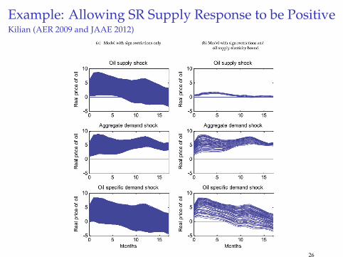
Example: Allowing SR Supply Response to be PositiveKilian (AER 2009 and JAAE 2012)

I Demand has large persistent effect on prices

26

Conclusion

I Time series analysts tend to ask questions that are less clean,perhaps because they have few clean experiments

I Rather than what is the effect of X and Y, askI What is the response of Y to an unexpected change in X? How

long does the response last?

I How does X vary?

I How much of the variation in Y does X explain?

I Think of the impulse respone as an average treatment effectI The treatment is a forecast error

I Track the response at various horizons

27