CRANFIELD UNIVERSITY

IBRAHIM NURUDDIN KATSINA

EFFECT OF WELDING THERMAL CYCLES ON THE HEAT

AFFECTED ZONE MICROSTRUCTURE AND TOUGHNESS OF

MULTI-PASS WELDED PIPELINE STEELS

SCHOOL OF APPLIED SCIENCES

WELDING ENGINEERING

PhD THESIS

Academic Year: 2011 - 2012

Supervisor: Dr Supriyo Ganguly and Mr David Yapp

September 2012

CRANFIELD UNIVERSITY

SCHOOL OF APPLIED SCIENCES

WELDING ENGINEERING

PhD

Academic Year 2011 - 2012

IBRAHIM NURUDDIN KATSINA

Effect of welding thermal cycles on the heat affected zone

microstructure and toughness of multi-pass welded pipeline steels

Supervisor: Dr Supriyo Ganguly and Mr David Yapp

September 2012

This thesis is submitted in fulfilment of the requirements for the

degree of PhD

© Cranfield University 2012. All rights reserved. No part of this

publication may be reproduced without the written permission of the

copyright owner.

i

ABSTRACT

This research is aimed at understanding the effect of thermal cycles on the

metallurgical and microstructural characteristics of the heat affected zone of a

multi-pass pipeline weld.

Continuous Cooling Transformation (CCT) diagrams of the pipeline steel grades

studied (X65, X70 and X100) were generated using a thermo mechanical

simulator (Gleeble 3500) and 10 mm diameter by 100 mm length samples. The

volume change during phase transformation was studied by a dilatometer, this

is to understand the thermodynamics and kinetics of phase formation when

subjected to such varying cooling rates. Samples were heated rapidly at a rate

of 400°C/s and the cooling rates were varied between t8/5 of 5.34°C/s to

1000°C/s. The transformation lines were identified using the dilatometric data,

metallographic analysis and the micro hardness of the heat treated samples.

Two welding processes, submerged arc welding (SAW) and tandem Metal Inert

Gas (MIG) Welding, with vastly different heat inputs were studied. An API-5L

grades X65, X70 and X100 pipeline steels with a narrow groove bevel were

experimented with both welding processes. The welding thermal cycles during

multi-pass welding were recorded using thermocouples.

The microstructural characteristics and metallurgical phase formation was

studied and correlated with the fracture toughness behaviour as determined

through the Crack Tip Opening Displacement (CTOD) tests on the welded

specimens. It was observed that SAW process is more susceptible to generate

undesirable martensite-austenite (M-A) phase which induce formation of

localised brittle zones (LBZ) which can adversely affect the CTOD performance.

Superimposition of the multiple thermal cycles, measured in-situ from the

different welding processes on the derived CCTs, helped in understanding the

mechanism of formation of localised brittle zones.

Charpy impact samples were machined from the two X65 and X70 grades, for

use in thermal simulation experiments using thermo mechanical simulator

(Gleeble). The real thermal cycles recorded from the HAZ of the SAW were

ii

used for the thermal simulations, in terms of heating and cooling rates. This is to

reproduce the microstructures of the welds HAZ in bulk on a charpy impact

sample which was used for impact toughness testing, hardness and

metallurgical characterisation.

The three materials used were showing different response in terms of the

applied thermal cycles and the corresponding toughness behaviours. The X65

(a) i.e. the seamless pipe was showing a complete loss of toughness when

subjected to the single, double and triple thermal cycles, while the X65 (b),

which is a TMCP material was showing excellent toughness in most cases

when subjected to the same thermal cycles at different test temperatures. The

X70 TMCP as well was showing a loss of toughness as compared to the X65

(b).

From the continuous cooling transformation diagrams and the thermally

simulated samples results it could be established that different materials

subjected to similar thermal cycle can produce different metallurgical phases

depending on the composition, processing route and the starting microstructure.

Keywords:

Thermal simulations, Gleeble 3500, submerged arc welding, Tandem MIG

welding, Continuous Cooling Transformation diagrams, Dilatometry, Phase

transformations, Charpy impact toughness, CTOD.

iii

ACKNOWLEDGEMENTS

In the name of Allah the beneficent the merciful. I wish to express my profound

gratitude to Allah (SWT) for his grace and mercy granted to me right form birth

to date, "Alhamdulillah."

My heartfelt gratitude goes to my parents, Alhaji Nuruddin Ibrahim and Hajiya

Binta Na'iya, and my wife Fadila and children Ja’afar and Muhammad Noor for

their support both morally and spiritually, and for their patience, love, guidance,

encouragement and prayers during this research period. May Allah have mercy

on them as they have mercy on me Ameen. Same goes to my brothers and

sisters for whose love, guidance, encouragement and prayers have seen me

through all the good and bad times.

My heartfelt gratitude goes to the Petroleum Technology Development Fund

(PTDF) and my employers Hassan Usman Katsina Polytechnic, Katsina for the

opportunity awarded to me to pursue a PhD at Cranfield University.

I wish to render my unreserved gratitude to my project supervisors Dr Supriyo

Ganguly and Mr David Yapp for their patience, care, guidance, and time given

to me during this research work. I will never forget it, thank you and God bless

you.

I will also like to show my appreciation to our technical staffs that have helped

me through the practical work, especially Mr Brian Brooks, Flemming Nielsen,

Andrew Dyer, Mathew Kershaw and Stuart Morse of University of Manchester

for his help with all the Gleeble machine experiments. I will also want to

acknowledge the help of Mr Alan Denney of Saipem UK, for his support during

this research.

My profound gratitude goes to my review chair, Dr Philip Longhurst and my

subject adviser Dr Paul Colegrove, and finally Professor Stewart Williams for

their care concern and support during the course of my research.

I wish to acknowledge the support and encouragement of my colleagues in the

office, especially Harry for his help with all the Matlab programs and Daniel for

iv

his help with office suite. Similar goes to Wojciech, Eurico, Mathew, Stephan,

Usani, Filomeno, Tamas, Craig, Isidro, Wang, Jibrin, Anthony, Adam, Fude,

Pedro, Goncalo and Sonia.

During the course of my stay at Cranfield I have met a lot of wonderful people,

some of whom I have shared my joys and sorrow with, noticeable among them

are Nuhu, Abdulkarim, B. Muneer, Muammer, Bello, Abba, Shinkafi, Murtala,

Sanusi, Sani, Abu, Abdussalam, Saif, Abu-Abdullah, Sami, Abdulmajid,

Sulaiman, Mubarak, Muhammad and Furjani (Rigima) among others numerous

to mention. I say to you all thank you very much and God bless you.

Finally, I am grateful to my lord Once again who has created me and makes it

possible with his mercy to witness this day and time, and to see the fruits of my

hard work and dedication.

"Alhamdu lillahil lazi bi ni’imatihi tatimmus-salihat".

v

TABLE OF CONTENTS

ABSTRACT ......................................................................................................... i

ACKNOWLEDGEMENTS................................................................................... iii

LIST OF FIGURES ............................................................................................. ix

LIST OF TABLES ............................................................................................. xix

LIST OF EQUATIONS ....................................................................................... xx

LIST OF ABBREVIATIONS .............................................................................. xxi

1 INTRODUCTION ............................................................................................. 1

2 LITERATURE REVIEW ................................................................................... 5

Background ............................................................................................... 5 2.1

Multi-pass welds, thermal cycles and microstructures .............................. 6 2.2

Martensite-Austenite constituents ........................................................... 10 2.3

2.3.1 M-A formation during multi-pass welding ......................................... 11

2.3.2 Identifying the M-A constituents ....................................................... 13

Phase transformation in pipeline steels .................................................. 24 2.4

2.4.1 Cooling rates during multi-pass welding and its effects on

metallurgical characteristics ...................................................................... 25

Inter-pass temperature ............................................................................ 26 2.5

Continuous cooling transformation (CCT) curve ..................................... 27 2.6

Dilatometric analysis ............................................................................... 29 2.7

HAZ simulation using Gleeble thermo mechanical simulator .................. 34 2.8

2.8.1 Modelling of weld simulation ............................................................ 35

Effect of different welding procedures on HAZ toughness ...................... 35 2.9

Effect of composition ............................................................................. 36 2.10

Recent advances .................................................................................. 38 2.11

Summary .............................................................................................. 39 2.12

3 AIMS AND OBJECTIVES .............................................................................. 41

Aim .......................................................................................................... 41 3.1

Specific research objectives ................................................................... 41 3.2

4 MATERIALS AND EQUIPMENTS ................................................................. 43

Materials ................................................................................................. 43 4.1

4.1.1 Pipeline steels .................................................................................. 43

4.1.2 Filler wires ........................................................................................ 45

4.1.3 Shielding gas .................................................................................... 45

4.1.4 Flux .................................................................................................. 46

Welding equipments ............................................................................... 47 4.2

4.2.1 Welding rig ....................................................................................... 47

4.2.2 Submerged arc welding power source ............................................. 48

4.2.3 Tandem MIG power source .............................................................. 49

Weld Instrumentation .............................................................................. 50 4.3

4.3.1 Thermal cycles acquisition during welding processes ...................... 50

vi

4.3.2 Capacitance discharge welder ......................................................... 52

4.3.3 Measurement of welding parameters ............................................... 52

Thermal simulation.................................................................................. 53 4.4

4.4.1 Gleeble machine .............................................................................. 53

4.4.2 Dilatometer ....................................................................................... 55

Characterisation ...................................................................................... 55 4.5

4.5.1 Metallographic examination .............................................................. 55

4.5.2 Micro hardness measurements ........................................................ 56

5 EXPERIMENTAL METHODS ........................................................................ 57

Dilatometric experiments (CCT Diagrams) ............................................. 58 5.1

Submerged arc welds ............................................................................. 60 5.2

5.2.1 Bead on plate welds ......................................................................... 60

5.2.2 Full submerged arc welds ................................................................ 63

Tandem MIG welds ................................................................................. 67 5.3

Thermal simulation (Gleeble) experiments ............................................. 70 5.4

5.4.1 Gleeble machine operation .............................................................. 72

Metallographic examination .................................................................... 73 5.5

Hardness measurements ........................................................................ 75 5.6

Tensile test ............................................................................................. 76 5.7

Charpy impact test .................................................................................. 77 5.8

Crack tip opening displacement test (CTOD) .......................................... 77 5.9

6 EXPERIMENTAL RESULTS ......................................................................... 79

Parent materials ...................................................................................... 79 6.1

6.1.1 Parent materials mechanical properties ........................................... 79

6.1.2 Parent materials microstructure ....................................................... 82

Dilatometric experiments (CCT Diagrams) ............................................. 86 6.2

6.2.1 Thermal cycles and dilatation curves ............................................... 86

6.2.2 Transformation start and finish temperatures ................................... 90

6.2.3 CCT Diagrams ................................................................................. 91

6.2.4 Microstructural characterisation of dilatometric samples .................. 93

6.2.5 Hardness versus t8/5 ....................................................................... 111

Submerged arc welding ........................................................................ 112 6.3

6.3.1 Bead on plate (BOP) welds ............................................................ 112

6.3.2 Full welds (Submerged arc welds) ................................................. 119

6.3.3 SAW hardness traverse across the welds ...................................... 135

6.3.4 Real thermal cycles of submerged arc welds HAZ ......................... 138

6.3.5 Crack tip opening displacement test (CTOD) results ..................... 139

6.3.6 Hardness maps of the notch area .................................................. 141

Tandem MIG welds ............................................................................... 144 6.4

6.4.1 Macrographs of tandem MIG welds ............................................... 144

6.4.2 Micrographs of tandem MIG welds ................................................. 145

6.4.3 Thermal cycles of the tandem MIG welds ...................................... 148

vii

6.4.4 Tandem MIG welds hardness traverses ......................................... 149

6.4.5 CTOD results of X70(a) tandem MIG welds ................................... 151

Thermal simulations .............................................................................. 153 6.5

6.5.1 Thermal cycles used for thermal simulation ................................... 153

6.5.2 Charpy impact test results .............................................................. 155

6.5.3 Fractography of the broken charpy impact samples ....................... 163

6.5.4 Microstructural characterisation of the charpy impact samples ...... 166

6.5.5 Hardness traverse of the charpy impact samples .......................... 170

6.5.6 Comparison of hardness (HV0.5) between the inner and the outer

surfaces................................................................................................... 173

7 DISCUSSION .............................................................................................. 175

Parent materials .................................................................................... 175 7.1

7.1.1 Parent materials mechanical and metallurgical analyses ............... 175

Dilatometric experiments (CCT Diagrams) ........................................... 177 7.2

7.2.1 Thermal cycles and dilatation for CCTs .......................................... 177

7.2.2 CCT Diagrams ............................................................................... 180

7.2.3 Hardness versus log t8/5 plots ......................................................... 190

7.2.4 Comparison between the four steels .............................................. 190

Submerged arc welding ........................................................................ 193 7.3

7.3.1 Bead on plate (BOP) welds ............................................................ 193

7.3.2 Full submerged arc welds .............................................................. 194

7.3.3 Effect of hardness on the CTOD .................................................... 198

7.3.4 SAW thermal cycles ....................................................................... 199

7.3.5 Superimposition of thermal cycles on the CCT curves to

understand phase evolution .................................................................... 202

7.3.6 Identifying M-A phases ................................................................... 206

Tandem MIG welds ............................................................................... 207 7.4

7.4.1 Tandem MIG macrostructures ........................................................ 207

7.4.2 Tandem MIG microstructures ......................................................... 207

7.4.3 Tandem MIG thermal cycles .......................................................... 208

7.4.4 CTOD results of the X70 tandem MIG welds ................................. 209

7.4.5 Probabilistic nature of the CTOD results ........................................ 209

Thermal simulations .............................................................................. 210 7.5

7.5.1 Thermal cycles used for the simulation .......................................... 210

7.5.2 Charpy impact results..................................................................... 211

7.5.3 Effect of cooling rates used on the charpy impact results .............. 215

7.5.4 Fractography of the broken charpy impact samples ....................... 215

7.5.5 Microstructural analysis of the broken charpy impact samples ...... 217

7.5.6 Characterization of M-A phase ....................................................... 220

7.5.7 Hardness traverses ........................................................................ 224

7.5.8 Comparison of hardness between inner and outer surfaces .......... 224

8 CONCLUSIONS .......................................................................................... 227

viii

9 RECOMMENDATIONS ............................................................................... 229

Recommendation to companies ........................................................... 229 9.1

Recommendation for future work .......................................................... 230 9.2

REFERENCES ............................................................................................... 231

APPENDICES ................................................................................................ 251

Appendix A Welding Parameters ................................................................ 251

Appendix B Gleeble experiments thermal cycles ........................................ 266

Appendix C MATLAB Programs ................................................................. 273

ix

LIST OF FIGURES

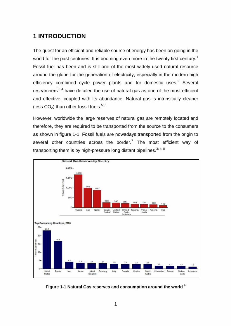
Figure 1-1 Natural Gas reserves and consumption around the world ................ 1

Figure 2-1 various microstructures produced by welding heat cycles ................ 6

Figure 2-2 Identification of microstructures of CTOD specimen (K-joint) ............ 8

Figure 2-3 Schematic comparison of the microstructures of (a) single run and (b) multi-run welds ....................................................................................... 9

Figure 2-4 SEM of an M-A constituent on the grain boundaries, 10,000× ........ 10

Figure 2-5 Illustration of fine structure of M-A island. ....................................... 12

Figure 2-6 TEM bright image of M-A island. ..................................................... 13

Figure 2-7 SEM micrograph after two step electrolytic etching showing (a) elongated M-A constituent, (b) Massive M-A constituent and (c) decomposed structure ............................................................................... 15

Figure 2-8 Typical mixed M-A island observed (after Villela etching) using FEG equipped scanning electron microscope operated at 1 kV ........................ 16

Figure 2-9 (a) High-strength dual-phase steel. 2% nital (b) same field as a, improved etchant. ...................................................................................... 18

Figure 2-10 (a) same sample as above 2% nital (b) same field as a, improved etchant. ..................................................................................................... 18

Figure 2-11 Three-dimensional optical micrograph showing, (a) as-deposited microstructure as revealed by 2% nital and (b) solidification segregation as revealed by modified LePèra Reagent. ..................................................... 19

Figure 2-12 Schematic illustration of Time-Resolved X-Ray Diffraction system set in the 46XU beam line in Spring-8. ...................................................... 21

Figure 2-13 Experimental setup for TRXRD experiments. ............................... 21

Figure 2-14 (a) is the schematic representation of static weld experiment where the arc was extinguished instantaneously, and (b) slope-down experiment where the arc current was reduced slowly from maximum value to zero in 25 s. Due to the decreasing current, arc movement took place and the weld pool shifted as shown in the inset. ............................................................ 22

Figure 2-15 Schematic diagram of high-temperature laser confocal microscope system ....................................................................................................... 23

Figure 2-16 Continuous cooling transformation diagram .................................. 27

Figure 2-17 A typical dilation curve at a cooling rate of 0.1°C/s with no clear vertices ...................................................................................................... 30

x

Figure 2-18 A DSC diagram at a cooling rate of 0.1°C/s showing clear transformation points ................................................................................. 30

Figure 2-19 A CCT diagram made by the use of dilatometric test, microstructural examination and DSC analyses. ....................................... 31

Figure 2-20 Dilatation curves of various cooling rates ...................................... 32

Figure 2-21 Heating dilatation curve of a low carbon steel at a very slow heating rate (0.05 K s-1) ......................................................................................... 32

Figure 2-22 Dilatometric representation of the splitting phenomena on the martensitic transformation of Cr13 and CrMoV14 stainless steels. ........... 33

Figure 2-23 Schematic layout of weld simulator equipment ............................. 34

Figure 3-1 Research flow chart ........................................................................ 42

Figure 4-1 Linear welding rig with an RMS welding head oscillator .................. 47

Figure 4-2 Travel speed calibration used for submerged arc welding .............. 48

Figure 4-3 STARMATIC 1300 DC submerged arc welding machine with a Subarc 5 and Mecacycle S controllers. ..................................................... 49

Figure 4-4 Fronius TPS 4000 thermo power welding machines ....................... 50

Figure 4-5 Thermocouple data acquisition device ............................................ 51

Figure 4-6 Capacitance discharge welder SR-48 ............................................. 51

Figure 4-7 AMV 4000 welding data logger ....................................................... 52

Figure 4-8 Gleeble 3500 thermal mechanical simulator ................................... 53

Figure 4-9 the heating chamber of the Gleeble 3500 simulator ........................ 54

Figure 4-10 QuickSim software window ........................................................... 54

Figure 4-11 High resolution dilatometer with a range of ± 2.5 mm ................... 55

Figure 4-12 Zwick Roell micro hardness testing machine ................................ 56

Figure 5-1 Outline of materials used for the various experiments .................... 57

Figure 5-2 Schematic of the dilatometric samples ............................................ 58

Figure 5-3 Dilatometer attached to the sample................................................. 59

Figure 5-4 Graphic representation of the dilatometric experiments .................. 59

Figure 5-5 Submerged arc welds bead on plate thermocouples positioning .... 61

Figure 5-6 Bead on plate welds set-up ............................................................. 63

Figure 5-7 Submerged arc welds narrow bevel design .................................... 64

xi

Figure 5-8 Submerged arc welds set-up .......................................................... 64

Figure 5-9 Submerged arc full welds thermocouples positioning ..................... 65

Figure 5-10 Thermocouples arrangements before submerged arc welding ..... 66

Figure 5-11 Flux holder .................................................................................... 67

Figure 5-12 Narrow groove (tandem MIG) bevel design .................................. 68

Figure 5-13 AutoCAD drawing of the tandem MIG welds thermocouple placement .................................................................................................. 69

Figure 5-14 Tandem MIG welds thermocouple arrangement ........................... 69

Figure 5-15 Schematic of the relative orientation of the samples with respect to the plates................................................................................................... 71

Figure 5-16 Schematic of the gleeble samples ................................................. 71

Figure 5-17 Gleeble thermocouple welder ....................................................... 72

Figure 5-18 Graphic representation of the gleeble experiments ....................... 73

Figure 5-19 Broken charpy sample showing where the metallographic samples were taken across section A – A ............................................................... 74

Figure 5-20 Schematic of full welds hardness traverse .................................... 75

Figure 5-21 Schematic of the full weld hardness map ...................................... 76

Figure 5-22 Gleeble sample hardness traverse ................................................ 76

Figure 6-1 Parent materials hardness values (HV0.5) ...................................... 79

Figure 6-2 Parent materials charpy impact toughness ..................................... 80

Figure 6-3 Parent materials tensile properties .................................................. 80

Figure 6-4 YS/UTS ratio of the parent materials ............................................... 81

Figure 6-5 Optical micrographs of all the parent materials (a) X65 (A), (b) X65 (B), (c) X70 and (d) X100 pipeline materials ............................................. 83

Figure 6-6 SEM Micrographs of all the parent materials (a) X65 (A), (b) X65 (B), (c) X70 and (d) X100 pipeline material ...................................................... 85

Figure 6-7 Thermal cycle recorded from the Gleeble machine for a fast cooling rate ............................................................................................................ 86

Figure 6-8 Thermal cycle recorded from the Gleeble machine for a slow cooling rate ............................................................................................................ 87

Figure 6-9 Dilatation curve recorded by a dilatometer for a fast cooling rate.... 87

Figure 6-10 Dilatation curve recorded by a dilatometer for a slow cooling rate 88

xii

Figure 6-11 A dilatation curve indicating the transformation start and finish, the AC1 and AC3 temperatures ......................................................................... 90

Figure 6-12 CCT diagram of X65 (A) ................................................................ 91

Figure 6-13 CCT diagram of X65 (B) ................................................................ 91

Figure 6-14 CCT diagram of X70 ..................................................................... 92

Figure 6-15 CCT diagram of X100 ................................................................... 92

Figure 6-16 Optical micrographs of X65 (A) steel after dilatometric cycles, cooled at t8/5 of (a) 6 s, (b) 6.4 s, (c) 15 s, (d) 25 s, (e) 50 s, (f) 90 s, (g) 250 s, (h) 1000 s, and their respective hardness HV0.5 .................................. 96

Figure 6-17 Optical micrographs of X65 (B) steel after dilatometric cycles, cooled at t8/5 of (a) 5.34 s, (b) 7.59 s, (c) 15 s, (d) 25 s, (e) 50 s, (f) 250 s, (g) 600 s, (h) 1000 s, and their respective hardness HV0.5 .................... 100

Figure 6-18 Optical micrographs of X70 steel after dilatometric cycles, cooled at t8/5 of (a) 7 s, (b) 7.8 s, (c) 10 s, (d) 15 s, (e) 25 s, (f) 90 s, (g) 400 s, (h) 1000 s and their respective hardness HV0.5........................................... 104

Figure 6-19 Optical micrographs of X100 steel after dilatometric cycles, cooled at t8/5 of (a) 5.34 s, (b) 6.29 s, (c) 15 s, (d) 25 s, (e) 50 s, (f) 250 s, (g) 600 s, (h) 1000 s, and their respective hardness HV0.5 ................................ 108

Figure 6-20 Optical micrographs of fast cooling rates (i) X65 (A) at t8/5 6s, (ii) X65 (B) at t8/5 5.34s, (iii) X70 at t8/5 7s and (iv) X100 at t8/5 5.34s ........... 109

Figure 6-21 Optical micrographs of slow cooling rates (i) X65 (A), (ii) X65 (B), (iii) X70 and (iv) X100 all at t8/5 of 1000s ................................................. 109

Figure 6-22 Optical micrographs of air quenched samples (a) X65 (A), (b) X65 (B), (c) X70 and (d) X100 ........................................................................ 110

Figure 6-23 Optical micrographs of oil quenched samples (a) X65 (A), (b) X65 (B), (c) X70 and (d) X100 ........................................................................ 110

Figure 6-24 Optical micrographs of Water quenched samples (a) X65 (A), (b) X65 (B), (c) X70 and (d) X100 ................................................................. 111

Figure 6-25 Hardness values against log of t8/5 .............................................. 111

Figure 6-26 Weld 1 BOP macrographs .......................................................... 112

Figure 6-27 Weld 2 BOP macrographs .......................................................... 113

Figure 6-28 Weld 3 BOP macrographs .......................................................... 113

Figure 6-29 Weld 4 BOP macrographs .......................................................... 113

Figure 6-30 SEM micrographs of the weld metal for (a) Weld 1, (b) Weld 2, (c) Weld 3 and (d) Weld 4 ............................................................................ 116

xiii

Figure 6-31 Hardness traverses along and across the weld beads ................ 117

Figure 6-32 Thermal cycles of the BOP welds for TC-1 at 10 mm and TC-5 at 17 mm from the bottom ........................................................................... 118

Figure 6-33 Macrographs of X65 (A) weld 1 ................................................... 119

Figure 6-34 Macrographs of X65 (A) weld 3 ................................................... 120

Figure 6-35 Macrographs of X65 (B) weld 1 ................................................... 120

Figure 6-36 Macrographs of X65 (B) weld 3 ................................................... 121

Figure 6-37 Macrograph of X70 weld 2 .......................................................... 121

Figure 6-38 Macrograph of X70 weld 3 .......................................................... 121

Figure 6-39 Optical micrographs of submerged arc welded X65 (A) showing from left to right; weld metal, fusion line and HAZ (15 mm from the bottom) at different magnifications ....................................................................... 122

Figure 6-40 Optical micrograph of SAW X65 (A) HAZ at 10 mm from the bottom ................................................................................................................ 123

Figure 6-41 Optical micrograph of SAW X65 (A) HAZ at 15 mm from the bottom ................................................................................................................ 123

Figure 6-42 SEM micrograph of SAW X65 (A) HAZ at 10 mm from the bottom ................................................................................................................ 124

Figure 6-43 SEM micrograph of SAW X65 (A) HAZ at 15 mm from the bottom ................................................................................................................ 124

Figure 6-44 Optical micrographs of SAW X65 (B) showing from left to right; weld metal, fusion line and HAZ (15 mm from the bottom) at different magnifications ......................................................................................... 125

Figure 6-45 SEM micrograph of SAW X65 (B) showing the HAZ ................... 126

Figure 6-46 SEM micrograph of SAW X65 (B) showing the microstructure of the thermocouple position ............................................................................. 126

Figure 6-47 Optical micrographs of SAW X70 showing from right to left; weld metal, fusion line and HAZ (15 mm from the bottom) at different magnifications ......................................................................................... 127

Figure 6-48 Optical Micrograph of SAW X70 showing fusion line and HAZ at 15 mm from the bottom ................................................................................ 128

Figure 6-49 Optical micrograph of SAW X70 showing the microstructure of the thermocouple position ............................................................................. 128

Figure 6-50 SEM micrograph of SAW X70 showing the HAZ at 15 mm from the bottom ..................................................................................................... 129

xiv

Figure 6-51 SEM micrograph of SAW X70 showing the microstructure of the thermocouple position ............................................................................. 129

Figure 6-52 Optical micrographs of X65 (A) SAW HAZ at 15 mm from the bottom, showing (a) Nital etch and (b) LePèra etched ............................ 130

Figure 6-53 Optical micrographs of X65 (B) SAW TC area at 10 mm from the bottom, showing (a) Nital etch and (b) LePèra etched ............................ 131

Figure 6-54 Optical micrographs of SAW X70 HAZ at 10 mm from the bottom, showing (a) Nital etch and (b) LePèra etched ......................................... 132

Figure 6-55 Optical micrographs of X70 tandem MIG HAZ at 10 mm from the bottom, showing (a) Nital etch and (b) LePèra etched ............................ 133

Figure 6-56 Optical micrographs of X100 tandem MIG HAZ at 10 mm from the bottom, showing (a) Nital etch and (b) LePèra etched ............................ 134

Figure 6-57 X65 (A) SAW hardness traverse across the welds...................... 135

Figure 6-58 X65 (B) SAW hardness traverse across the welds...................... 136

Figure 6-59 X70 SAW hardness traverse across the welds ........................... 137

Figure 6-60 Representative thermal cycles of SAW full welds on X70 pipes . 138

Figure 6-61 Macrographs of X70 SAW Welds CTOD (a) weld 1 and (b) weld 2 ................................................................................................................ 140

Figure 6-62 Pictures of the CTOD samples broken faces of X70 SAW (a) weld 1 and (b) weld 2 ......................................................................................... 140

Figure 6-63 X65 (A) SAW weld 1 hardness map ............................................ 141

Figure 6-64 X65 (A) SAW weld 3 hardness map ............................................ 141

Figure 6-65 X65 (B) SAW weld 1 hardness map ............................................ 142

Figure 6-66 X65 (B) SAW weld 3 hardness map ............................................ 142

Figure 6-67 X70 SAW weld 1 hardness map ................................................. 143

Figure 6-68 X70 SAW weld 2 hardness map ................................................. 143

Figure 6-69 Macrographs of tandem MIG X70 weld 1 .................................... 144

Figure 6-70 Macrographs of tandem MIG X70 weld 2 .................................... 144

Figure 6-71 Optical micrographs of X70 tandem MIG welds, showing from left to right; weld metal, fusion line and HAZ (15 mm from the top) at different magnifications ......................................................................................... 145

Figure 6-72 Optical micrograph of X70 tandem MIG weld showing the microstructure of the thermocouple position............................................ 146

xv

Figure 6-73 Optical micrograph of X100 tandem MIG weld, showing from left to right; weld metal, fusion line and HAZ at the middle of the weld ............. 146

Figure 6-74 SEM micrograph of X70 tandem MIG weld 1 HAZ at 15 mm from the top, showing (a) secondary electrons and (b) backscattered electrons ................................................................................................................ 147

Figure 6-75 Representative thermal cycles of narrow groove tandem MIG welds, on X100 pipe ................................................................................ 148

Figure 6-76 Hardness traverse across the narrow groove tandem MIG welds on X70 .......................................................................................................... 149

Figure 6-77 Hardness traverse across the narrow groove tandem MIG welds on X100 ........................................................................................................ 150

Figure 6-78 X70 tandem MIG weld 1 hardness map ...................................... 152

Figure 6-79 X70 tandem MIG weld 2 hardness map ...................................... 152

Figure 6-80 Single thermal cycle from the Gleeble machine data .................. 153

Figure 6-81 Double thermal cycle from the Gleeble machine data ................. 154

Figure 6-82 Triple thermal cycle from the Gleeble machine data ................... 154

Figure 6-83 Charpy impact results of the single thermal cycles for X65 (A), X65 (B) and X70 at the same cooling rates .................................................... 155

Figure 6-84 Charpy impact results of the double thermal cycles at intercritical temperatures (below AC3) for X65 (A) and X65 (B) at the same cooling rate ................................................................................................................ 156

Figure 6-85 Charpy impact results of the double thermal cycles at intercritical temperatures (below AC3) for X70 at a different cooling rate ................... 156

Figure 6-86 Charpy impact results of the double thermal cycles at supercritical temperatures (above AC3) for X65 (A), X65 (B) and X70 at the same cooling rates ........................................................................................................ 157

Figure 6-87 Charpy impact results of the triple thermal cycles for X65 (A), X65 (B) and X70 at the same cooling rates .................................................... 158

Figure 6-88 Comparison of the charpy impact results at different second peak temperatures with cooling rates for X65 (A) ............................................ 159

Figure 6-89 Comparison of the charpy impact results at different second peak temperatures with cooling rates for X65 (B) ............................................ 160

Figure 6-90 Comparison of the charpy impact results at different second peak temperatures with cooling rates for X70 .................................................. 161

Figure 6-91 Effect of cooling rate on the charpy impact results for X70 ......... 162

xvi

Figure 6-92 Fractographs of X65 (A) single thermal cycles at peak temperatures of (a) 1250°C and (b) 1000°C ................................................................. 163

Figure 6-93 Fractographs of X65 (B) single thermal cycles at peak temperatures of (a) 1250°C and (b) 1000°C ................................................................. 163

Figure 6-94 Fractographs of X70 single thermal cycles at peak temperatures of (a) 1250°C and (b) 1000°C ..................................................................... 163

Figure 6-95 Fractographs of X65 (A) second thermal cycles of 1000° at cooling rates of (a) 17.5°C/s and (b) 20°C/s ........................................................ 164

Figure 6-96 Fractographs of X65 (B) second thermal cycles of 1000° at cooling rates of (a) 17.5°C/s and (b) 20°C/s ........................................................ 164

Figure 6-97 Fractographs of X70 second thermal cycles of 1000° at cooling rates of (a) 17.5°C/s and (b) 20°C/s ........................................................ 164

Figure 6-98 Fractographs of X65 (A) third thermal cycles with peak temperatures of (a) 450°C and (b) 350°C ............................................... 165

Figure 6-99 Fractographs of X65 (B) third thermal cycles with peak temperatures of (a) 450°C and (b) 350°C ............................................... 165

Figure 6-100 Fractographs of X70 third thermal cycles with peak temperatures of (a) 450°C and (b) 350°C ..................................................................... 165

Figure 6-101 SEM micrographs of X65 (A) single thermal cycles at peak temperatures of (a) 1250°C and (b) 1000°C ........................................... 166

Figure 6-102 SEM micrographs of X65 (B) single thermal cycles at peak temperatures of (a) 1250°C and (b) 1000°C ........................................... 166

Figure 6-103 SEM micrographs of X70 single thermal cycles at peak temperatures of (a) 1250°C and (b) 1000°C ........................................... 166

Figure 6-104 Optical micrographs of X65 (A) single thermal cycles at peak temperatures of (a) 1250°C and (b) 1000°C ........................................... 167

Figure 6-105 Optical micrographs of X65 (B) single thermal cycles at peak temperatures of (a) 1250°C and (b) 1000°C ........................................... 167

Figure 6-106 Optical micrographs of X70 single thermal cycles at peak temperatures of (a) 1250°C and (b) 1000°C ........................................... 167

Figure 6-107 Optical micrographs of X65 (A) double thermal cycles with a second peak temperature of 1000°C, at cooling rates of (a) 17.5°C/s and (b) 20°C/s ................................................................................................ 168

Figure 6-108 Optical micrographs of X65 (B) double thermal cycles with a second peak temperature of 1000°C, at cooling rates of (a) 17.5°C/s and (b) 20°C/s ................................................................................................ 168

xvii

Figure 6-109 Optical micrographs of X70 double thermal cycles with a second peak temperature of 1000°C, at cooling rates of (a) 17.5°C/s and (b) 20°C/s ................................................................................................................ 168

Figure 6-110 Optical micrographs of X65 (A) triple thermal cycles with third peak temperatures of (a) 450°C and (b) 350°C ....................................... 169

Figure 6-111 Optical micrographs of X65 (B) triple thermal cycles with third peak temperatures of (a) 450°C and (b) 350°C ....................................... 169

Figure 6-112 Optical micrographs of X70 triple thermal cycles with third peak temperatures of (a) 450°C and (b) 350°C ............................................... 169

Figure 6-113 Hardness comparison on X65 (A) single thermal cycles, between inner and outer surfaces ......................................................................... 173

Figure 6-114 Hardness comparison on X65 (B) double thermal cycles, between inner and outer surfaces ......................................................................... 173

Figure 7-1 Continuous heating part of a dilatation curve ................................ 178

Figure 7-2 Cooling dilatation curve ................................................................. 180

Figure 7-3 X65 (a) CCT diagram with various transformation lines identified . 182

Figure 7-4 Optical micrograph of water quenched samples (a) X65 (A), (b) X65 (B), (c) X70 and (d) X100 ........................................................................ 183

Figure 7-5 X65 (b) CCT diagram with transformation lines identified ............. 184

Figure 7-6 X70 CCT diagram showing the transformation lines identified ...... 186

Figure 7-7 Micrographs of the fastest cooling rates for (i) X65 (a) at t8/5 = 6 s, (ii) X65 (b) at t8/5 = 5.34 s, (iii) X70 at t8/5 = 7 s, (iv) X100 at t8/5 = 5.34 s ...... 187

Figure 7-8 Micrographs of the slowest cooling rate (0.3°C/s) for (i) X65 (a), (ii) X65 (b), (iii) X70 and (iv) X100 all at t8/5 of 1000 s .................................. 188

Figure 7-9 X100 CCT diagram indicating the transformation lines identified .. 189

Figure 7-10 Relationship between the transformation start temperature of different materials and the cooling rates ................................................. 191

Figure 7-11 Relationship between the transformation finish temperature of different materials and the cooling rates ................................................. 192

Figure 7-12 Hardness traverse along the X70 SAW samples from top to bottom ................................................................................................................ 198

Figure 7-13 SAW TC arrangements showing thermocouples locations ......... 199

Figure 7-14 SAW X70 weld 3 TC-1 thermal cycles and the intercritical temperatures ........................................................................................... 200

xviii

Figure 7-15 SAW X70 weld 3 TC-3 thermal cycles and the intercritical temperatures ........................................................................................... 201

Figure 7-16 Superimposition of thermal cycles of weld 3 TC-1 on the CCT of the parent material ........................................................................................ 203

Figure 7-17 Superimposition of thermal cycles of weld 3 TC-3 on the CCT of the parent material ........................................................................................ 204

Figure 7-18 Relationship between heat input and peak temperature for X70 weld 3 TC-1 ............................................................................................. 205

Figure 7-19 Relationship between heat input and peak temperature for X70 weld 3 TC-3 ............................................................................................. 205

Figure 7-20 Optical micrographs of (a) real weld CGHAZ and (b) simulated CGHAZ for X65 (a) material .................................................................... 218

Figure 7-21 M-A phase on the fractographs of X70 triple thermal cycles (i) 450°C and (ii) 350°C ............................................................................... 221

Figure 7-22 SEM micrographs of X70, double thermal cycle samples at a second peak temperature of 1000°C and cooling rates of (i) 17.5°C/s and (ii) 20°C/s ................................................................................................ 222

Figure 7-23 Higher magnification SEM micrographs of X70, double thermal cycle samples at a second peak temperature of 1000°C and cooling rates of (i) 17.5°C/s and (ii) 20°C/s showing the M-A phases .......................... 223

Figure 7-24 Influence of second peak temperature on the hardness values of X65 (a), X65 (b) and X70 grades ............................................................ 225

xix

LIST OF TABLES

Table 4-1 Chemical composition of the pipeline steel grades. ......................... 44

Table 4-2 Chemical composition of the filler wires ........................................... 45

Table 4-3 Composition of Lincoln 888 flux from the manufacturer ................... 46

Table 4-4 Composition of OP 121TT flux from the manufacturer ..................... 46

Table 5-1 BOP weld names and number of passes on each weld ................... 61

Table 5-2 Submerged arc welds bead on plate welding parameters ................ 62

Table 6-1 Cooling rates, t8/5 and hardness values recorded from the CCT samples ..................................................................................................... 89

Table 6-2 Experimental and calculated transformation temperatures .............. 90

Table 6-3 Heat input for the BOP welds on X65 (A) ....................................... 114

Table 6-4 CTOD results of the HAZ from selected welds ............................... 139

Table 6-5 CTOD results of the HAZ from the X70 tandem MIG welds ........... 151

Table 6-6 Hardness traverse HV0.5 (Average) for the X65 (A) charpy impact samples ................................................................................................... 170

Table 6-7 Hardness traverse HV0.5 (Average) for the X65 (B) charpy impact samples ................................................................................................... 171

Table 6-8 Hardness traverse HV0.5 (Average) for the X70 charpy impact samples ................................................................................................... 172

Table 7-1 Mechanical properties requirements for the parent materials ......... 176

Table 7-2 X65 (a) thermal cycles and the corresponding hardness values .... 182

Table 7-3 X65 (b) thermal cycles and the corresponding hardness values .... 184

Table 7-4 X70 thermal cycles and the corresponding hardness values ......... 186

Table 7-5 X100 thermal cycles and the corresponding hardness values ....... 189

Table 7-6 Thermal cycles data from the BOP welds ...................................... 194

xx

LIST OF EQUATIONS

(2-1) .................................................................................................................... 7

(2-2) .................................................................................................................... 8

(2-3) .................................................................................................................. 24

(2-4) .................................................................................................................. 37

(2-5) .................................................................................................................. 37

(2-6) .................................................................................................................. 38

(2-7) .................................................................................................................. 38

xxi

LIST OF ABBREVIATIONS

a crack length

ac critical crack extension

B thickness of CTOD test specimen

CEV carbon equivalent

CR cooling rate

CTOD crack tip opening displacement

CTOA crack tip opening angle

CVN charpy V notch test

CGHAZ coarse grain heat affected zone

DJ double joint

FAD failure assessment diagram

FCGR fatigue crack growth rate

FGHAZ fine grain heat affected zone

GMAW gas metal arc welding

GTAW gas tungsten arc welding

HI heat input

HAZ heat affected zone

IR infrared

ICHAZ intercritical heat affected zone

ICRCGHAZ intercritically reheated coarse grain heat affected zone

J crack tip J-integral

Jc critical J at the onset of brittle crack extension when ∆a < 0.2 mm

xxii

JIc critical J near the onset of stable crack extension

Jm J at first attainment of maximum F plateau for full plastic behavior

Ju critical J at the onset of brittle crack extension when ∆a ≥ 0.2 mm

K stress intensity factor

KIc plane strain fracture toughness

LBZ local brittle zone

LM lamellar martensite

LVDT linear variable differential transducers

M-A martensite-austenite

MIG metal inert gas

RICC roughness induced crack closure

SAW submerged arc welding

SBCCGHAZ subcritical coarse grain heat affected zone

SCRCGHAZ supercritically reheated coarse grain heat affected zone

SENB single edge notched bend specimen

SPCCGHAZ supercritical coarse grain heat affected zone

SRXRD spatially resolved X-ray diffraction

t8/5 cooling time from 800°C to 500°C

TC thermocouples

TMCP thermo-mechanically controlled processing

TRXRD time resolved X-ray diffraction

UACGHAZ unaltered coarse grain heat affected zone

UFAF ultrafine acicular ferrite

xxiii

VHN vickers hardness number

V notch opening displacement

Vp plastic component of V

W CTOD specimen width

WM weld metal

XRD X-ray diffraction

δ crack tip opening displacement (CTOD)

δc critical δ at the onset of brittle crack extension when ∆a < 0.2 mm

δm δ at the first attainment of maximum F plateau for fully plastic

behavior

δu critical δ at the onset of brittle crack extension when ∆a ≥ 0.2 mm

1

1 INTRODUCTION

The quest for an efficient and reliable source of energy has been on going in the

world for the past centuries. It is booming even more in the twenty first century.1

Fossil fuel has been and is still one of the most widely used natural resource

around the globe for the generation of electricity, especially in the modern high

efficiency combined cycle power plants and for domestic uses.2 Several

researchers3; 4 have detailed the use of natural gas as one of the most efficient

and effective, coupled with its abundance. Natural gas is intrinsically cleaner

(less CO2) than other fossil fuels.5; 6

However, worldwide the large reserves of natural gas are remotely located and

therefore, they are required to be transported from the source to the consumers

as shown in figure 1-1. Fossil fuels are nowadays transported from the origin to

several other countries across the border.7 The most efficient way of

transporting them is by high-pressure long distant pipelines.3; 4; 8

Figure 1-1 Natural Gas reserves and consumption around the world 9

2

Welding is the most preferred and productive of all the joining process, to join

these long distant cross-country pipelines. However, unlike other joining

techniques, it produces an integrated structure with newly formed fusion and

heat affected zones. The metallurgical characteristics of the fusion and heat

affected zones are completely different from the parent material. This is due to

the heat from the process which causes grain growth, precipitates formation

and dissociation of carbides. This leads to formation of a graded structure.

The thermo mechanical controlled processing (TMCP) route, presents a

cheaper and more effective means of producing these pipeline steel. Therefore,

it was commonly adopted by pipeline manufactures, as a strengthening

technique.10; 11 The strength is achieved by producing very fine grains,12; 13 and

various carbides and nitrides or a combination of both within the microstructure.

These precipitates tend to reduce the grain size by hindering the grain boundary

movement, thereby making grain growth almost impossible.14

However, welding changes the microstructure of these steels due to the

formation of heat affected zone. Thermal cycles exceeding the transformation

temperatures in the HAZ, lead to a significant loss of toughness. This is due to

grain growth as a result of carbides dissolution, forming the coarse grain HAZ.

While in multi-pass welds, the intercritically re-heated coarse grain HAZ is

formed. The re-heated zones produce some unwanted islands, so called

martensite austenite (M-A) constituents, leading to the formation of local brittle

zones (LBZ). 15-19

Due to criticality (onshore, offshore, high pressures, natural and manmade

disasters etc.) of the application, it is required to understand how a crack or

defect will interact with the microstructure and propagate.20 The welded

structure has to undergo a stringent toughness, crack tip opening displacement

(CTOD) test. A small localised brittle zone in the entire weld can result in failure

to qualification of a weldment and in turn a welding process. To meet the set

standards, repairs are normally carried out on defective welds. This is costing

the industries both time and money.

3

In this research, we are trying to understand how the thermal cycles from a real

weld, can results in the formation of M-A phase, and its effect. Apprehend its

effect on the fracture toughness of the welds. Then simulate those thermal

cycles on charpy samples. This will produce a bulk microstructure with similar

properties for fracture toughness testing, and for both mechanical and

microstructural characterisations.

This thesis contains a total of nine chapters, where chapter 1 is the introduction.

Chapter 2 is the literature review, where the findings in this research area have

been discussed critically. Chapter 3 presents the aims and objectives of this

research work. This has been derived after synthesizing the data obtained from

the literature review.

Chapter 4 contains all the materials and equipments used in this research. The

experimental set-ups and how they were carried out was presented in chapter

5. The results were presented in chapter 6, and it contains the results obtained

from the experiments only. Chapter 7 presents a full discussion about the

results.

The conclusions and recommendations for future work are presented in

chapters 8 and 9 respectively. Finally the references and appendices are

presented at the end of the thesis.

5

2 LITERATURE REVIEW

Background 2.1

The search for even more efficient, reliable and cleaner source of energy has

been on for decades.21 Improvements through research and development have

been the main factor in achieving the desired results. A lot of research6; 22 has

taken place with regards to finding an economical and productive way of

transporting these natural resources. Pipelines have been the crucial answer to

the problem. They must be welded to one another and laid either onshore or

offshore to be able to transport these resources.23-25

The welding processes have been optimized in many respects such as process

parameters, shielding gas, consumables, weld preparation or bevel etc, in order

to get the most productive and cost effective means of joining these pipes.26-29

Modern steel manufacturing techniques has made it possible to optimize the

production routes. This requires changing the microstructures to obtain an

excellent combination of strength and toughness.30-35

There are certain problems associated with welding these pipeline steels,

especially the modern high strength low alloy steels (HSLA) or the thermo-

mechanically controlled processed steels (TMCP).6; 15; 36-40 41 This is due to their

production sequence which results in to very fine grains. It causes some

deleterious effects on the HAZ properties when welded.

Research papers15-19 over years have recognized that the loss in toughness of

the HAZ can be due to the following reasons.

(i) Formation of CGHAZ (Coarse grained heat affected zone)

(ii) Formation of ICCGHAZ (Intercritical coarse grained heat affected

zone)

(iii) Reheated ICCGHAZ (Reheated intercritical coarse grained HAZ)

These have been related to local brittle zone formation, and will be explained in

detail later in this review.

6

Multi-pass welds, thermal cycles and microstructures 2.2

The thermal cycles of multi-pass welds have a significant influence on the

mechanical and the metallurgical properties of the welded joints.42 They are

usually the cause of local brittle zones, which were believed to be due to the

presence of M-A islands.43; 44

Zalazar et al.45 evaluate the metallurgical phases that originate from pipeline

steel welds by using multi-pass welds at low heat inputs. Despite using low heat

input in their studies, local brittle zones could not be avoided. This is as a result

of the complex mechanism involving thermal cycles and compositional effects.

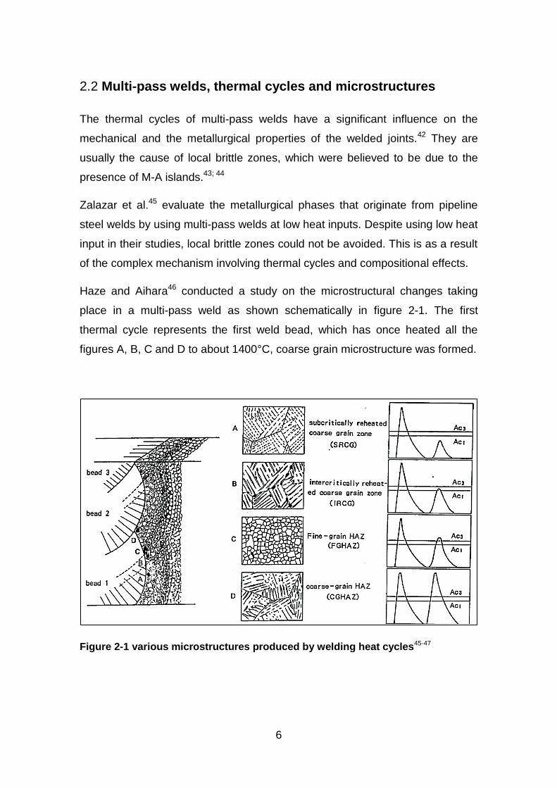
Haze and Aihara46 conducted a study on the microstructural changes taking

place in a multi-pass weld as shown schematically in figure 2-1. The first

thermal cycle represents the first weld bead, which has once heated all the

figures A, B, C and D to about 1400°C, coarse grain microstructure was formed.

Figure 2-1 various microstructures produced by welding heat cycles45-47

7

Figure A has been reheated just below the AC1 and is called the subcritically

reheated coarse grain (SRCG) zone. The base structure remains, but the

second phase may decompose, i.e. the microstructure is annealed.

In figure B the reheating temperature was between the inter-critical temperature

regions i.e. AC1 and AC3. It is called the intercritically reheated coarse grain

(IRCG) zone. Partial re-austenitization occurs at local regions with high carbon

contents, and there is a high tendency of forming brittle microstructures (M-A

island). This critical region normally exists at about 3 mm from the fusion line of

the first pass,45 depending on the welding process.

When the temperature crosses the AC3 line as seen in figure C, it is referred to

as supercritically reheated fine grain (SCFG) zone. Complete re-austenitization

occurs, but the peak temperature is not high enough to promote grain growth.

Therefore, the microstructure becomes normalised or refined.

At figure D, the reheating has gone well above AC3 line; the high temperature

promotes grain growth. This region is called the coarse grain (CG) zone, and

produces a coarse grained microstructure.

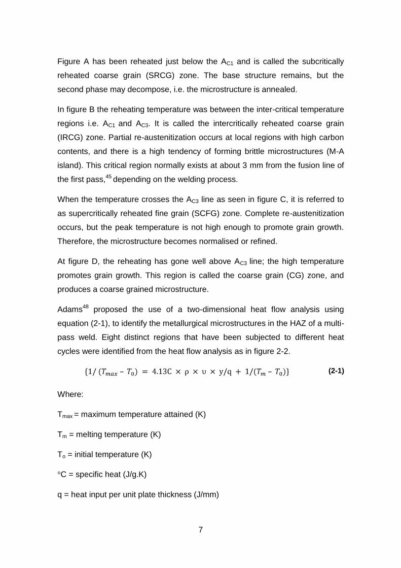
Adams48 proposed the use of a two-dimensional heat flow analysis using

equation (2-1), to identify the metallurgical microstructures in the HAZ of a multi-

pass weld. Eight distinct regions that have been subjected to different heat

cycles were identified from the heat flow analysis as in figure 2-2.

(2-1)

Where:

Tmax = maximum temperature attained (K)

Tm = melting temperature (K)

To = initial temperature (K)

°C = specific heat (J/g.K)

q = heat input per unit plate thickness (J/mm)

8

υ = welding speed (mm/s)

ρ = density (f/mm3)

y = distance from fusion line (mm)

Equation (2-1) was simplified to

(2-2)

Where A is a constant, determined using Tmax = 1173K, Tm =1823K, and y is the

HAZ width.47; 48 The following regions were classified as local brittle zones (LBZ)

sites:

1. The coarse grain HAZ (CGHAZ)

2. Subcritically reheated coarse grain HAZ (SRCG HAZ)

3. Intercritically reheated coarse grain HAZ (IRCG HAZ)

4. Tempered intercritically reheated coarse grain HAZ (TIRCG HAZ)

Figure 2-2 Identification of microstructures of CTOD specimen (K-joint) 47

9

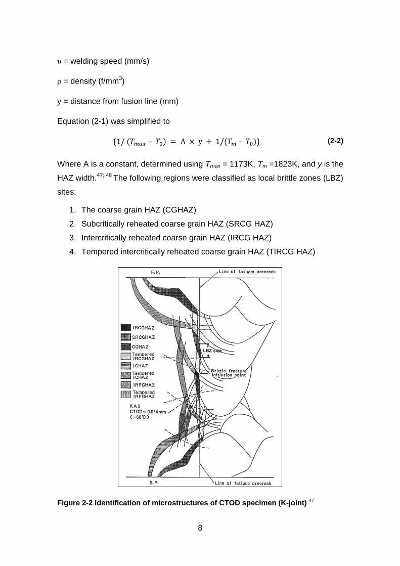
Multi-pass weld holds some excellent properties such as microstructural

refinement, better toughness and less residual stresses compared to single

pass weld. This is because: 49

- The thermal cycle from subsequent passes refine the grains from the

previous pass

- Total heat input per weld pass is reduced, therefore grain growth is

effectively reduced

- Previous passes provide some preheating effect that tends to extend the

critical cooling time of Δt8/5

- The subsequent passes has an annealing effect on the previous one,

thereby relieving residual stresses from the previous passes

Figure 2-3 is a schematic comparison between a single pass weld and a multi

pass weld.

The correct prediction of microstructure and hardness of the HAZ in multi-pass

welds of high strength steels are very important in optimizing the design of a

pipeline project with respect to weldability. The development of thermo-

microstructural models such as TENWELD© have been a welcome

development.50

Figure 2-3 Schematic comparison of the microstructures of (a) single run and (b)

multi-run welds49

10

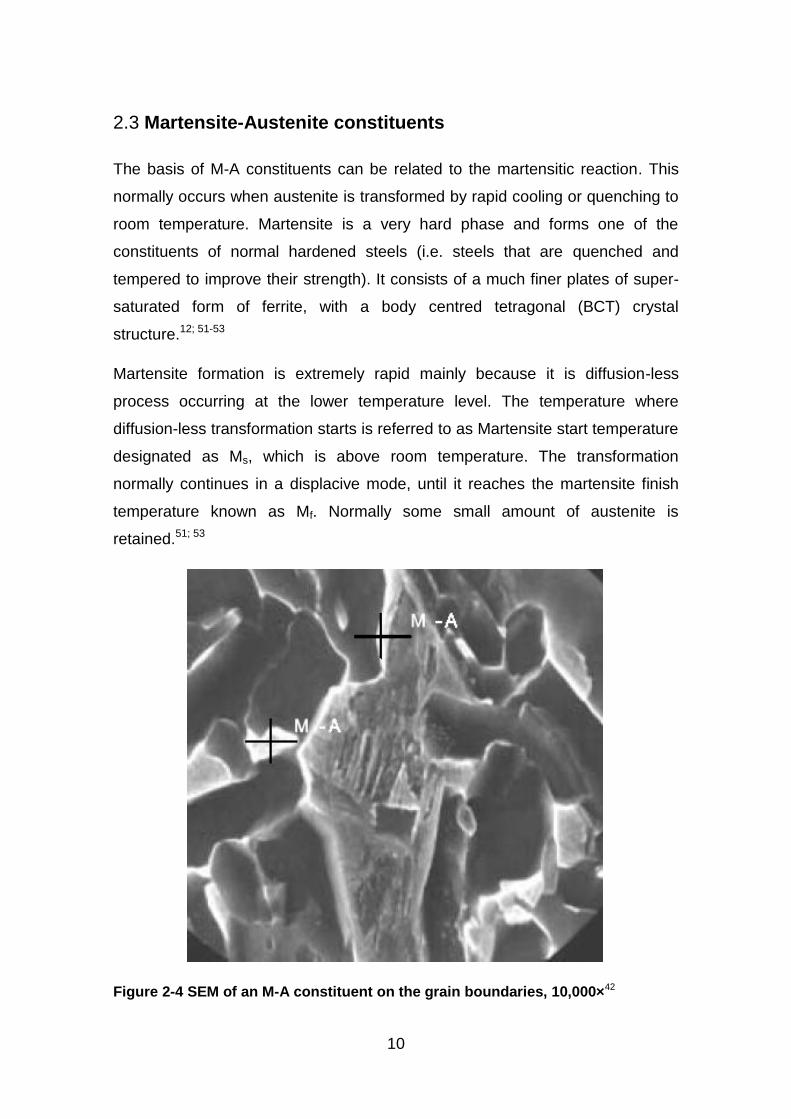
Martensite-Austenite constituents 2.3

The basis of M-A constituents can be related to the martensitic reaction. This

normally occurs when austenite is transformed by rapid cooling or quenching to

room temperature. Martensite is a very hard phase and forms one of the

constituents of normal hardened steels (i.e. steels that are quenched and

tempered to improve their strength). It consists of a much finer plates of super-

saturated form of ferrite, with a body centred tetragonal (BCT) crystal

structure.12; 51-53

Martensite formation is extremely rapid mainly because it is diffusion-less

process occurring at the lower temperature level. The temperature where

diffusion-less transformation starts is referred to as Martensite start temperature

designated as Ms, which is above room temperature. The transformation

normally continues in a displacive mode, until it reaches the martensite finish

temperature known as Mf. Normally some small amount of austenite is

retained.51; 53

Figure 2-4 SEM of an M-A constituent on the grain boundaries, 10,000×42

11

In welding, there is rapid cooling due to heat sink by the surrounding material

and the environment. Depending on the thermal cycles, formation of martensite

in the HAZ might be inevitable. This also varies from one material to another,

and depends on grain size, cooling rate, carbon equivalent and hardenability

among others. In the case of high strength steels their fine grained structure has

an influence on the transformation when subjected to different thermal cycles.

The mode by which martensite and bainite are formed has been found to affect

mechanical properties of materials. This has been explored by Bhadeshia.54

High magnification SEM micrograph with M-A phase identified on it is shown in

figure 2-4.

2.3.1 M-A formation during multi-pass welding

There has been an intensive research6; 38; 55; 56 which looked at the problems of

welding high strength steels. Emphasis was given to the formation of these

deleterious phase i.e. M-A phase or constituents. There are several theories of

formation and effects of M-A on the HAZ of pipeline welds.

For the past three decades, Ikawa et al.52 have made a scrupulous research in

identifying the theory behind the formation of M-A constituents. They come up

with an acceptable explanation of how the M-A phases are being formed upon

cooling of the material from austenitic state. Bainitic ferrite is obtained first,

while the remaining austenite becomes stable due to carbon enrichment.57; 58

This takes place at about 400-350°C, with a carbon content of about 0.5 - 0.8%.

Upon continuous cooling, at the range of 350-300°C part of the austenite tends

to transform in to ferrite and carbides. But under instantaneous cooling, this

process will never take place, whereby the un-decomposed austenite transform

in to twin and lath martensite at a lower temperature, while diminutive amount of

austenite is retained. Part of the reason been the compressive stresses

imposed by the surrounding acicular ferrite.42 In other words, the remaining

austenite is strained as the transformation induces volume change (increase in

volume). Therefore, the remaining austenite becomes strained. This is generally

referred to as the M-A constituents. 52; 59

12

Lambert et al.20 also explain the formation of M-A constituents in similar

manner, agreeing with the above theory, i.e. upon continuous cooling, there

was a partial transformation of the austenite in to martensite, leading to the

formation of M-A islands.

Chunming et al.5 investigate the formation of M-A islands in X70 pipeline steel

by using TEM. The result of their thermo-mechanical simulation test shows that

M-A islands were formed during the continuous cooling phase.

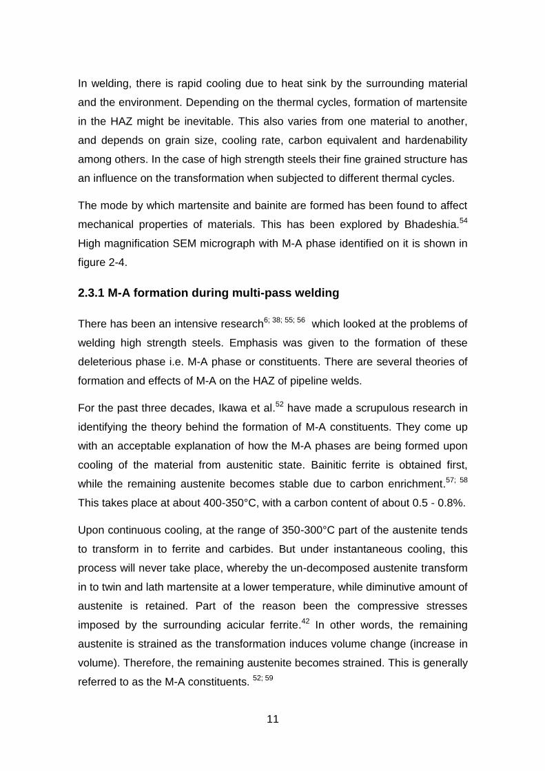
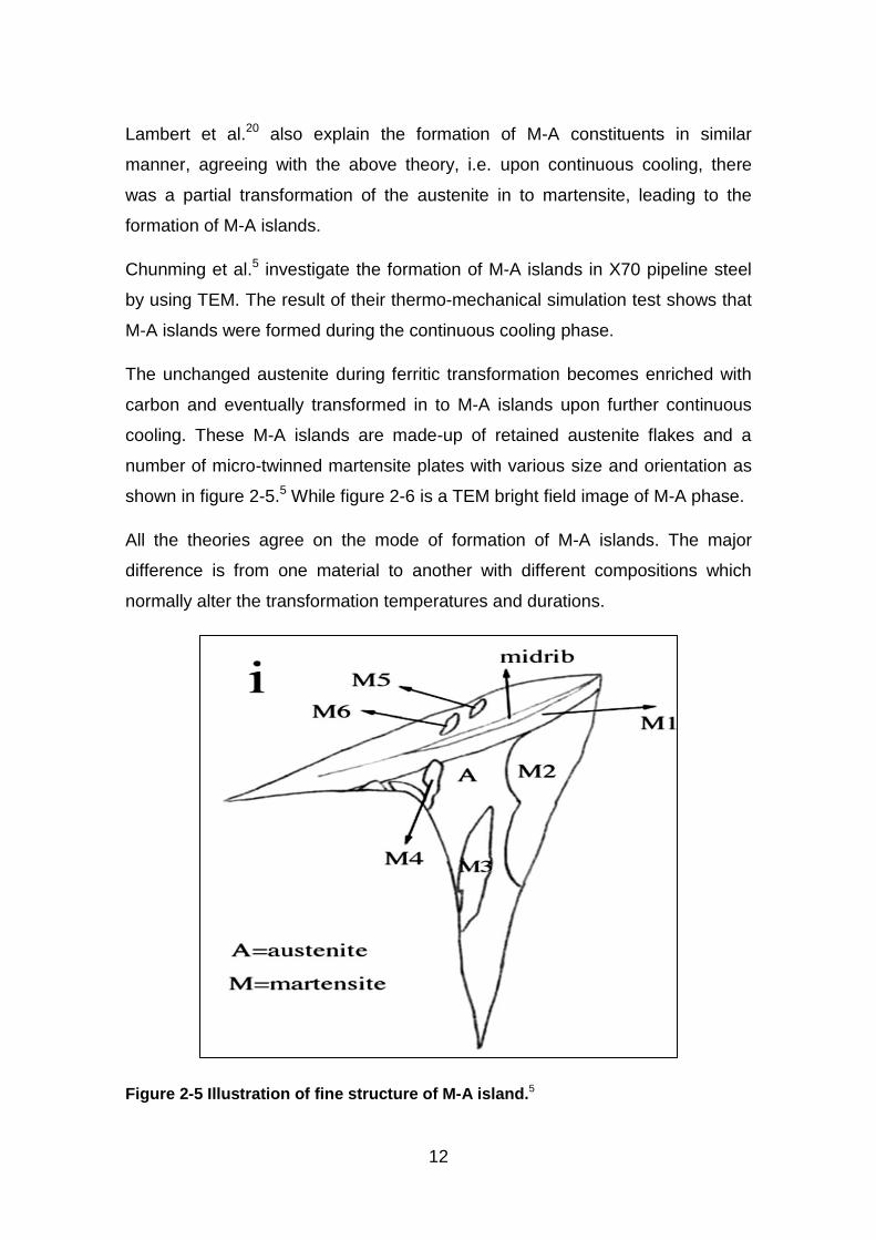
The unchanged austenite during ferritic transformation becomes enriched with

carbon and eventually transformed in to M-A islands upon further continuous

cooling. These M-A islands are made-up of retained austenite flakes and a

number of micro-twinned martensite plates with various size and orientation as

shown in figure 2-5.5 While figure 2-6 is a TEM bright field image of M-A phase.

All the theories agree on the mode of formation of M-A islands. The major

difference is from one material to another with different compositions which

normally alter the transformation temperatures and durations.

Figure 2-5 Illustration of fine structure of M-A island.5

13

Figure 2-6 TEM bright image of M-A island.5

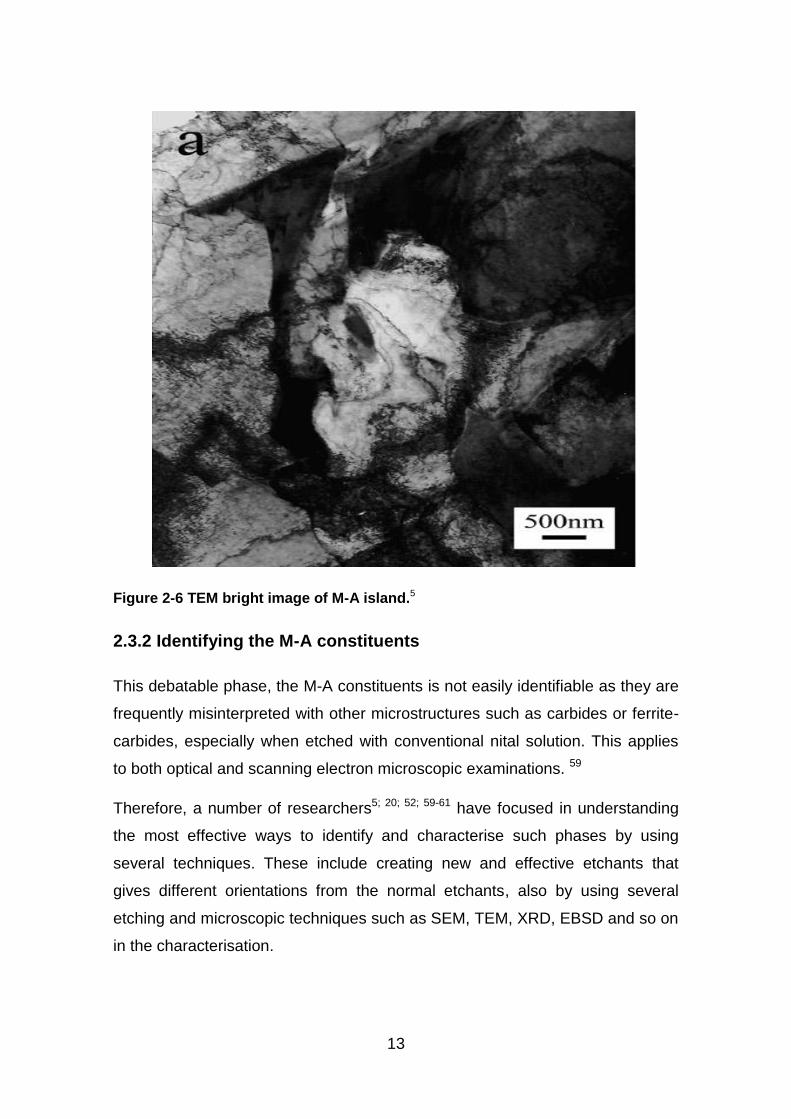
2.3.2 Identifying the M-A constituents

This debatable phase, the M-A constituents is not easily identifiable as they are

frequently misinterpreted with other microstructures such as carbides or ferrite-

carbides, especially when etched with conventional nital solution. This applies

to both optical and scanning electron microscopic examinations. 59

Therefore, a number of researchers5; 20; 52; 59-61 have focused in understanding

the most effective ways to identify and characterise such phases by using

several techniques. These include creating new and effective etchants that

gives different orientations from the normal etchants, also by using several

etching and microscopic techniques such as SEM, TEM, XRD, EBSD and so on

in the characterisation.

14

2.3.2.1 Etching techniques

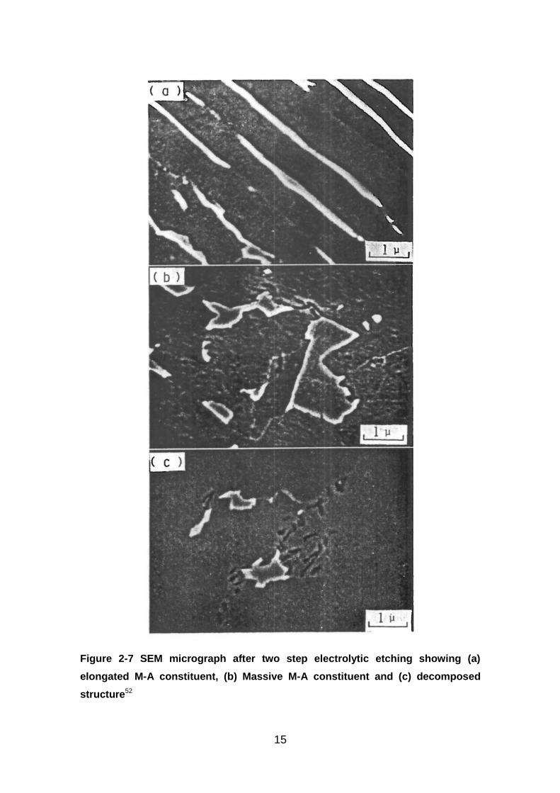
Two step electrolytic etching

Some of the researchers 52; 59 have demonstrated the possibility of using two-

step Metallographic etching technique in order to characterise between M-A

constituents and carbides. Ikawa et al.52 explained the technique behind the two

step electrolytic etching.

Ethylene diamine tetra acetic acid (EDTA) 5 g, sodium fluoride (NaF) 0.5 g and

distilled water 100 ml was used as the first etchant. 3 volts and 3 seconds were

used as the etching conditions. This method is excellent in etching the ferrite

while leaving the M-A constituents and carbides unetched.

Subsequently, picric acid 5 g, sodium hydroxide (NaOH) 25 g and distilled water

100 ml were used as electrolytes for the second stage etching, with 6 volts and

30 seconds etching conditions.

This second stage tends to etch carbides preferentially, such that after the two

stage etching, the M-A constituents are embossed and carbides are depressed

in a ferritic matrix. This makes it easier to distinguish between M-A constituents

and carbides when inspected in SEM as shown in figure 2-7.

15

Figure 2-7 SEM micrograph after two step electrolytic etching showing (a)

elongated M-A constituent, (b) Massive M-A constituent and (c) decomposed

structure52

16

Villela’s reagent

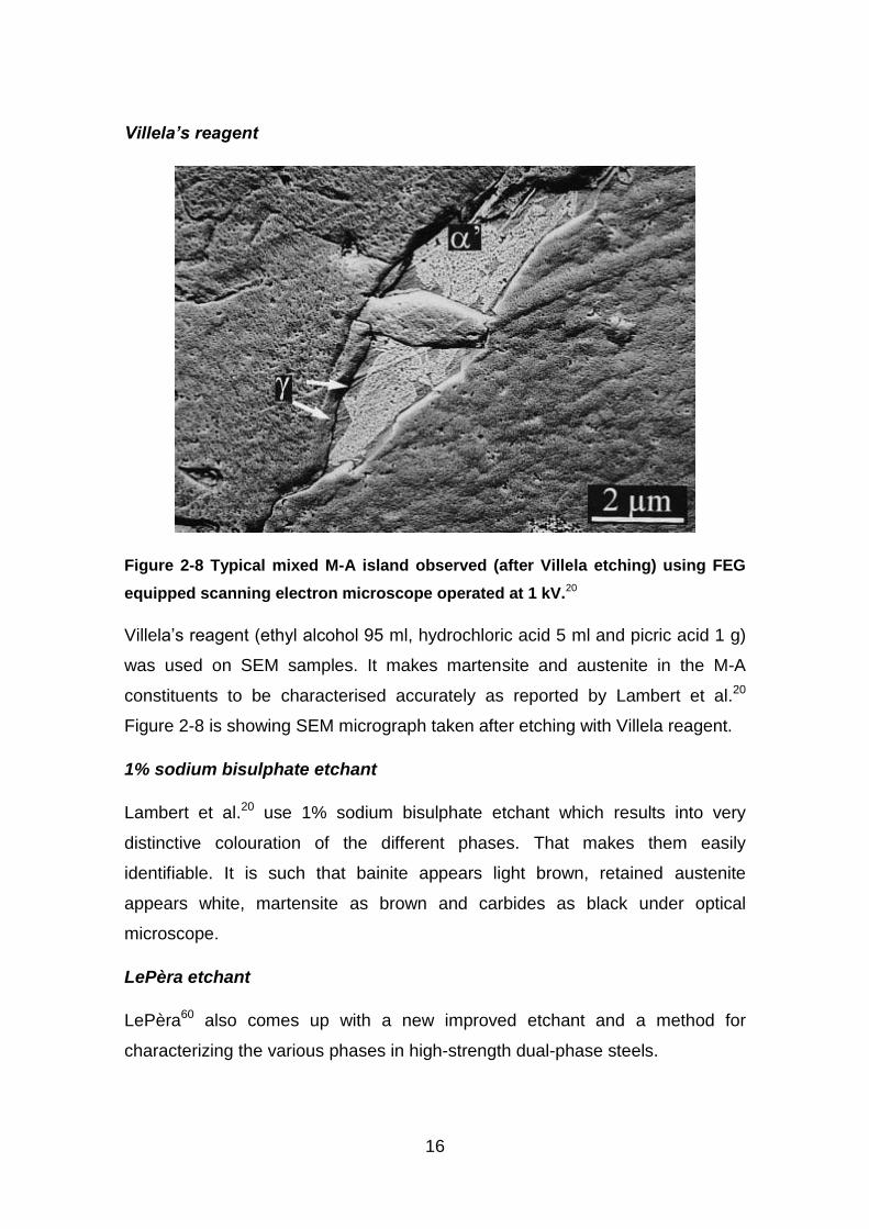
Figure 2-8 Typical mixed M-A island observed (after Villela etching) using FEG

equipped scanning electron microscope operated at 1 kV.20

Villela’s reagent (ethyl alcohol 95 ml, hydrochloric acid 5 ml and picric acid 1 g)

was used on SEM samples. It makes martensite and austenite in the M-A

constituents to be characterised accurately as reported by Lambert et al.20

Figure 2-8 is showing SEM micrograph taken after etching with Villela reagent.

1% sodium bisulphate etchant

Lambert et al.20 use 1% sodium bisulphate etchant which results into very

distinctive colouration of the different phases. That makes them easily

identifiable. It is such that bainite appears light brown, retained austenite

appears white, martensite as brown and carbides as black under optical

microscope.

LePèra etchant

LePèra60 also comes up with a new improved etchant and a method for

characterizing the various phases in high-strength dual-phase steels.

17

Conventional techniques and etching procedures have certain limitations when

micrographs were taken for electronic image analysis. In such circumstances,

often, specimens are tempered or over etched in order to get sufficient contrast

during image analysis. This may cause some of the phase constituents e.g.

bainite and grain boundaries to look similar (assume same shade) during

micrograph observation.

It was found that using 1% aqueous sodium-meta-bisulfite (Na2S2O) and 4%

picric acid in ethyl alcohol in a 1:1 ratio produced excellent contrast. This

eliminates the need for tempering or over etching.

The technique for preparing the specimen is such that the normal grinding

methods are used. But the final polishing is done in a series of polishing and

short etching treatments (5-7 sec) with 2% nital to remove any deformed metal.

Caution has to be taken to remove completely the nital etch before using

LePèra etchant. This is because any traces of the nital on the specimen

appears passive to the etchant. Therefore the final polishing needs to be done

twice longer to ensure there is no more nital on the specimen. The etchant is

then mixed and used immediately by immersing the sample for 7-12 seconds at

room temperature. This shows a kind of effervescent reaction at the surface

during the etching process. Finally the specimen is rinsed with ethyl alcohol and

blown dry. The surface should appear as blue-orange.

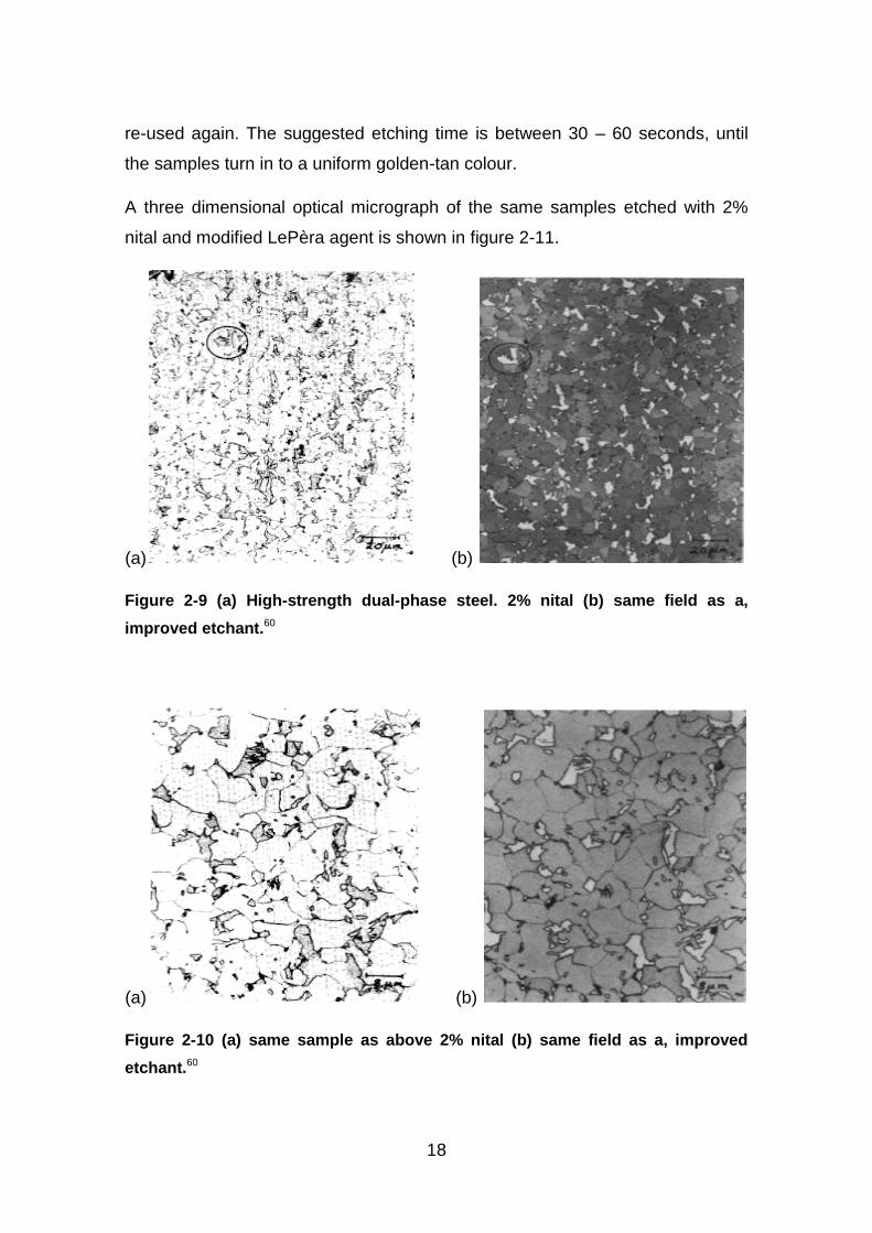
Figure 2-9 and figure 2-10 are showing optical micrographs of a high strength

dual phase steel etched with both nital and LePèra etchants. The same position

was etched with the two reagents for comparison.

Modified LePèra reagent

The quest for characterizing these phases leads Clark et al.62 to modify the

LePèra reagent. They use a new mixing formula with a volume ratio of 1:2 (4%

picral: 1% aqueous sodium-meta-bisulfite). This differs from LePèra with a

mixing ratio of 1:1. They found it to be more effective for HSLA 100 steel. The

mixture must be prepared just before etching, and discarded after, i.e. not to be

18

re-used again. The suggested etching time is between 30 – 60 seconds, until

the samples turn in to a uniform golden-tan colour.

A three dimensional optical micrograph of the same samples etched with 2%

nital and modified LePèra agent is shown in figure 2-11.

(a) (b)

Figure 2-9 (a) High-strength dual-phase steel. 2% nital (b) same field as a,

improved etchant.60

(a) (b)

Figure 2-10 (a) same sample as above 2% nital (b) same field as a, improved

etchant.60

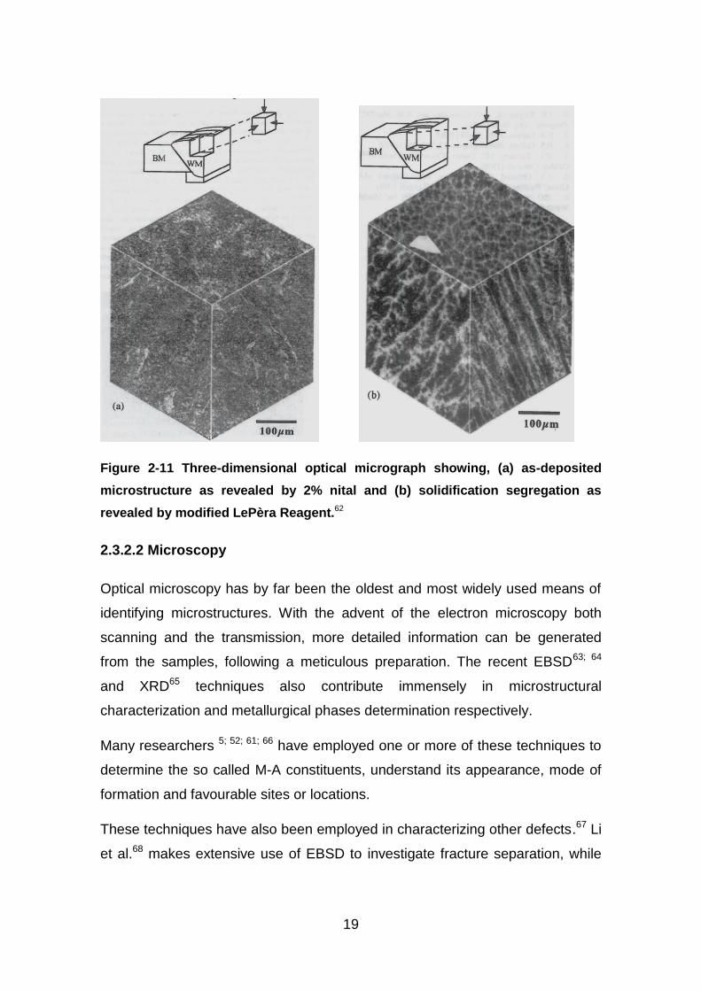
19

Figure 2-11 Three-dimensional optical micrograph showing, (a) as-deposited

microstructure as revealed by 2% nital and (b) solidification segregation as

revealed by modified LePèra Reagent.62

2.3.2.2 Microscopy

Optical microscopy has by far been the oldest and most widely used means of

identifying microstructures. With the advent of the electron microscopy both

scanning and the transmission, more detailed information can be generated

from the samples, following a meticulous preparation. The recent EBSD63; 64

and XRD65 techniques also contribute immensely in microstructural

characterization and metallurgical phases determination respectively.

Many researchers 5; 52; 61; 66 have employed one or more of these techniques to

determine the so called M-A constituents, understand its appearance, mode of

formation and favourable sites or locations.

These techniques have also been employed in characterizing other defects.67 Li

et al.68 makes extensive use of EBSD to investigate fracture separation, while

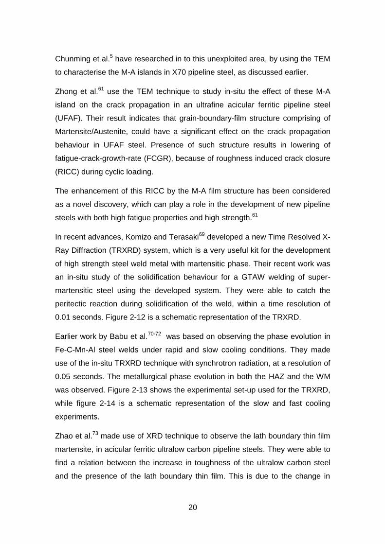
20

Chunming et al.5 have researched in to this unexploited area, by using the TEM

to characterise the M-A islands in X70 pipeline steel, as discussed earlier.

Zhong et al.61 use the TEM technique to study in-situ the effect of these M-A

island on the crack propagation in an ultrafine acicular ferritic pipeline steel

(UFAF). Their result indicates that grain-boundary-film structure comprising of

Martensite/Austenite, could have a significant effect on the crack propagation

behaviour in UFAF steel. Presence of such structure results in lowering of

fatigue-crack-growth-rate (FCGR), because of roughness induced crack closure

(RICC) during cyclic loading.

The enhancement of this RICC by the M-A film structure has been considered

as a novel discovery, which can play a role in the development of new pipeline

steels with both high fatigue properties and high strength.61

In recent advances, Komizo and Terasaki69 developed a new Time Resolved X-

Ray Diffraction (TRXRD) system, which is a very useful kit for the development

of high strength steel weld metal with martensitic phase. Their recent work was

an in-situ study of the solidification behaviour for a GTAW welding of super-

martensitic steel using the developed system. They were able to catch the

peritectic reaction during solidification of the weld, within a time resolution of

0.01 seconds. Figure 2-12 is a schematic representation of the TRXRD.

Earlier work by Babu et al.70-72 was based on observing the phase evolution in

Fe-C-Mn-Al steel welds under rapid and slow cooling conditions. They made

use of the in-situ TRXRD technique with synchrotron radiation, at a resolution of

0.05 seconds. The metallurgical phase evolution in both the HAZ and the WM

was observed. Figure 2-13 shows the experimental set-up used for the TRXRD,

while figure 2-14 is a schematic representation of the slow and fast cooling

experiments.

Zhao et al.73 made use of XRD technique to observe the lath boundary thin film

martensite, in acicular ferritic ultralow carbon pipeline steels. They were able to

find a relation between the increase in toughness of the ultralow carbon steel

and the presence of the lath boundary thin film. This is due to the change in

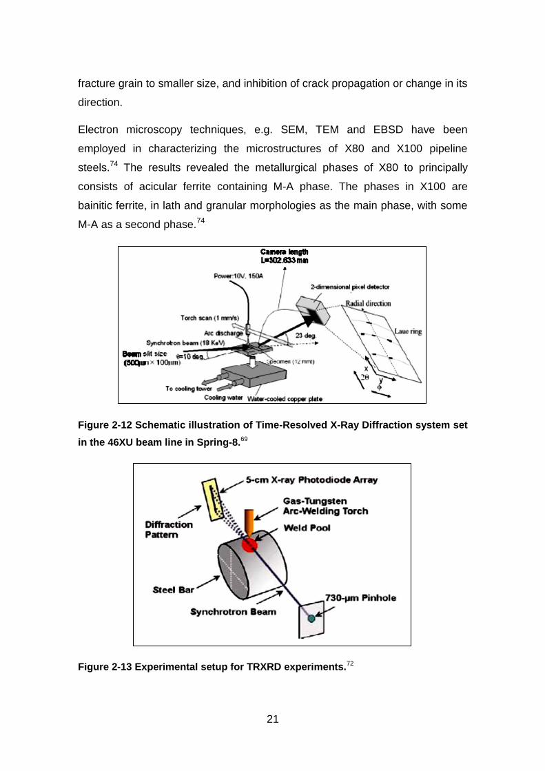
21

fracture grain to smaller size, and inhibition of crack propagation or change in its

direction.

Electron microscopy techniques, e.g. SEM, TEM and EBSD have been

employed in characterizing the microstructures of X80 and X100 pipeline

steels.74 The results revealed the metallurgical phases of X80 to principally

consists of acicular ferrite containing M-A phase. The phases in X100 are

bainitic ferrite, in lath and granular morphologies as the main phase, with some

M-A as a second phase.74

Figure 2-12 Schematic illustration of Time-Resolved X-Ray Diffraction system set

in the 46XU beam line in Spring-8.69

Figure 2-13 Experimental setup for TRXRD experiments.72

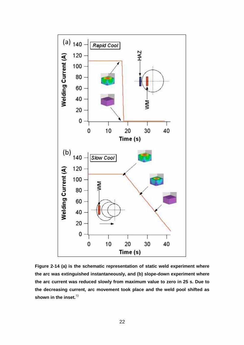
22

Figure 2-14 (a) is the schematic representation of static weld experiment where

the arc was extinguished instantaneously, and (b) slope-down experiment where

the arc current was reduced slowly from maximum value to zero in 25 s. Due to

the decreasing current, arc movement took place and the weld pool shifted as

shown in the inset.72

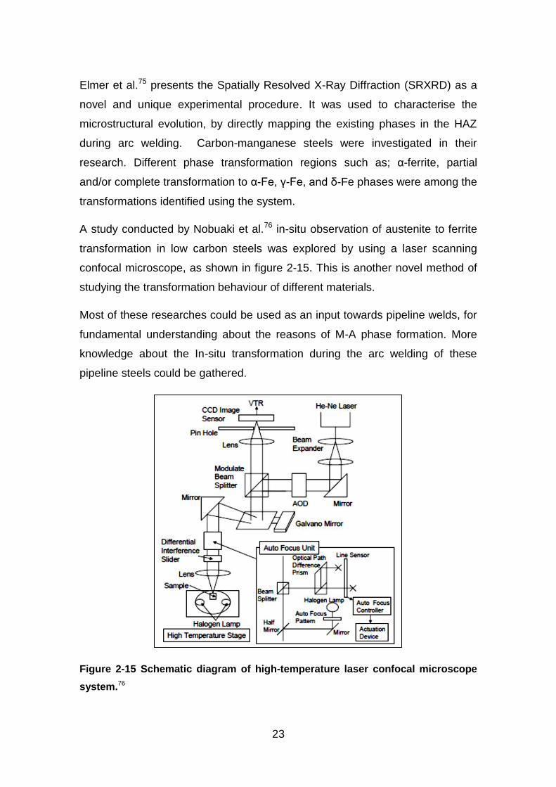
23

Elmer et al.75 presents the Spatially Resolved X-Ray Diffraction (SRXRD) as a

novel and unique experimental procedure. It was used to characterise the

microstructural evolution, by directly mapping the existing phases in the HAZ

during arc welding. Carbon-manganese steels were investigated in their

research. Different phase transformation regions such as; α-ferrite, partial

and/or complete transformation to α-Fe, γ-Fe, and δ-Fe phases were among the

transformations identified using the system.

A study conducted by Nobuaki et al.76 in-situ observation of austenite to ferrite

transformation in low carbon steels was explored by using a laser scanning

confocal microscope, as shown in figure 2-15. This is another novel method of

studying the transformation behaviour of different materials.

Most of these researches could be used as an input towards pipeline welds, for

fundamental understanding about the reasons of M-A phase formation. More

knowledge about the In-situ transformation during the arc welding of these

pipeline steels could be gathered.

Figure 2-15 Schematic diagram of high-temperature laser confocal microscope

system.76

24

Phase transformation in pipeline steels 2.4

The understanding of phase transformation in pipeline steels is vital.77 Due to

the nature of their applications, i.e. under different terrains and operational

conditions, pipeline steels requires a matching combination of strength and

toughness. These properties are achieved through various processing and heat

treatment routes, which gives different phase combinations and microstructural

condition. Therefore a sound knowledge of phase transformation is necessary

to understand the effect of welding heat on these pipeline steels.42; 78; 79

Knowledge of grain growth and nucleation during phase transformations help to

develop materials with excellent mechanical properties.57 Due to the nature of

welding thermal cycle, the weld metal cools very fast, losing heat to the

environment and the neighbouring base metal. This leads to the formation of

heat affected zones.

This rapid cooling leads to non-equilibrium conditions, resulting in strain induced

solid state phase transformation.70 In pipeline steels welds, the condition is like

normal solidification of a cast metal.80 A cellular-dendritic structure is obtained,

which consist of coarse and columnar austenitic grains that curve into the weld

centre line, with a fine cellular network within the grains.49

Grain nucleation and growth are very important in polycrystalline materials, i.e.

metals. During processing, they control the kinetics of different phase

transformations and recrystallization processes.

The final grain size determines the strength of the material. Generally smaller

average grain sizes results in a stronger material, such as these high strength

steels.57 This has been explained by equation (2-3) termed as Hall- Petch

equation. Where d is the average grain diameter, σo and ky are constants for a

particular material.81

(2-3)

25

Phase transformation during welding is generally controlled by a number of

factors which include, the composition of both the base and filler metals,

metallurgical processes occurring at different interfaces, and the thermo-

mechanical histories during the welding process.49

The general approaches for investigating phase transformations in welding

have been classified into two: In-vitro and In-situ.82

In-vitro, which simply means simulation of the welding thermal cycles on some

standard specimens that could be used for further mechanical and

microstructural analysis, have been in use since the late 40’s by Nippes and

Savage.83

While in-situ means using a real weld to measure the thermal history at a

particular point, with the use of thermocouples or other non-contact methods

such as infrared84 and/or thermal cameras. Accurate capturing of thermal cycles

(temperature vs. time) and differential analysis of the same are used in

determination of start and finish of the phase transformation.82

On-going researches have shown the viability of other thermal analysis

methods in determining the phase transformation temperatures in welding, such

as single sensor differential thermal analysis.85

2.4.1 Cooling rates during multi-pass welding and its effects on

metallurgical characteristics

Phase transformations are influenced by the cooling rates experienced by the

weld metal and associated HAZ from the different welding process variables.70

Given the wide range of cooling rates taking place during the solidification of

steel welds, it is likely that the first phase to form is not in an equilibrium

condition.70 This leads to the formation of different kinds of phases and thus

affects the mechanical properties.

Studies78; 86-90 have been carried out to understand the effect of different cooling

rates on metallurgical and mechanical properties of pipeline steel welds.

26

Recent work by Keehan et al.91 explores the effect of cooling rate on

microstructure and properties of high strength steel welds.

Shi and Han92 used simulated thermal cycle specimens to show the effect of

cooling time and peak temperatures on fracture toughness and microstructure.

They found in their work that the best toughness was obtained at a cooling time

t8/5 of 18 s. Also the volume fraction of M-A constituent increases with increase

in cooling time, while that of martensite decreases with increase in cooling time.

The microstructural characterisation of API 5L X80 pipeline steels subjected to

different thermal cycles was evaluated by Bott et al.93 they subjected the steels

samples to an austenitization temperature of 900°C for an hour, then cooled at

three different rates of 1.5°C/s, 30°C/s and 115°C/s using air, oil and water

respectively. They looked at the effects of these thermal cycles on the

hardness, tensile strength, grain size and phases.

Inter-pass temperature 2.5

Inter-pass temperature can be referred to as the temperature both minimum

and maximum, of the preceding pass and adjacent base metal just before the

successive pass during a multi-pass weld.94 It has a very strong relation with the

mechanical and metallurgical properties of a weld, it also influences the

distortions. Inter-pass temperature depends on the composition of the material

and the cooling rate of the weld.95

As explained by Jones and Luo96 the preheating range is based on various

factors such as; chemical composition and physical properties of the weld

piece, the thickness of the weld pieces, electrode type, heat input and the level

of standards needed. The control of preheat and inter-pass temperatures

reduces the effect of residual stress and cooling rates imposed by the welding

process, and thus the metallurgical phases formed.97 Preheating temperature

can be calculated using the carbon equivalent, which shows the possibility of

martensite formation in a particular material.98

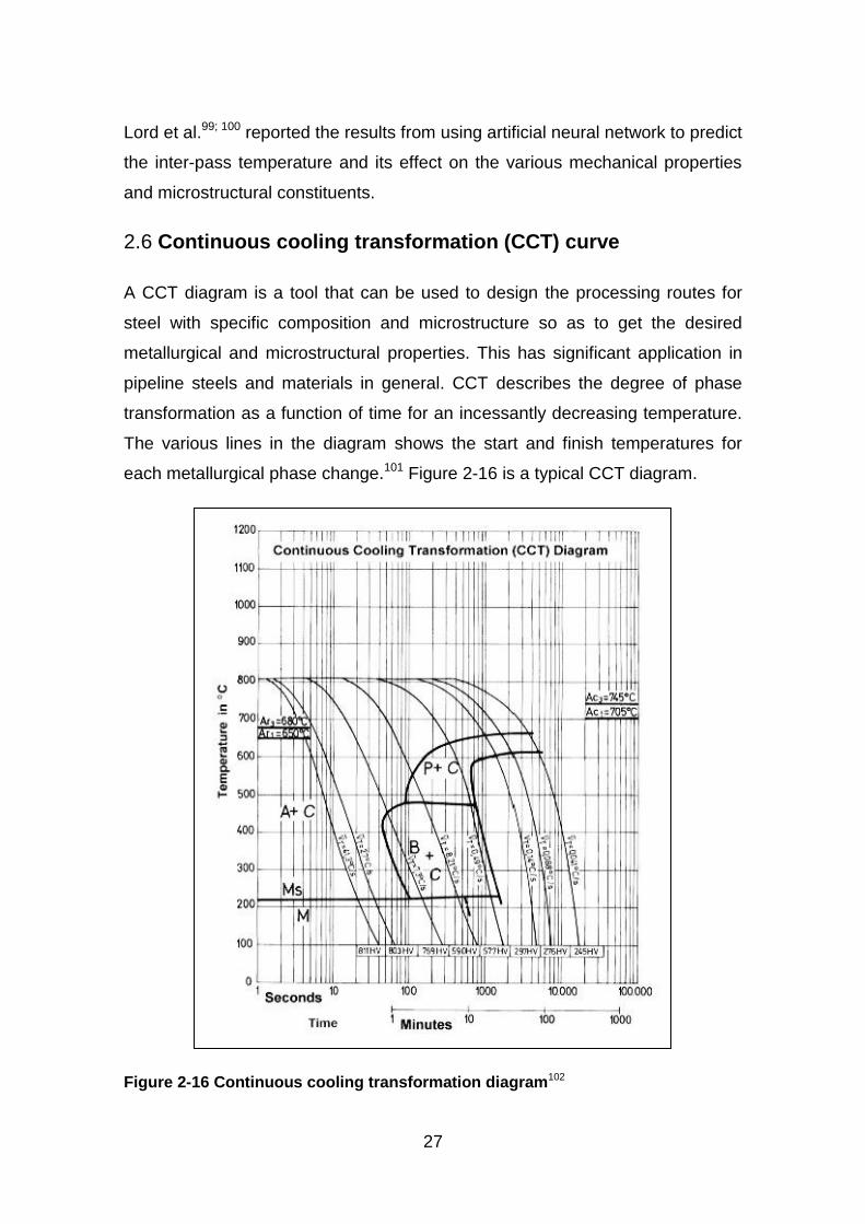
27

Lord et al.99; 100 reported the results from using artificial neural network to predict

the inter-pass temperature and its effect on the various mechanical properties

and microstructural constituents.

Continuous cooling transformation (CCT) curve 2.6

A CCT diagram is a tool that can be used to design the processing routes for

steel with specific composition and microstructure so as to get the desired

metallurgical and microstructural properties. This has significant application in

pipeline steels and materials in general. CCT describes the degree of phase

transformation as a function of time for an incessantly decreasing temperature.

The various lines in the diagram shows the start and finish temperatures for

each metallurgical phase change.101 Figure 2-16 is a typical CCT diagram.

Figure 2-16 Continuous cooling transformation diagram102

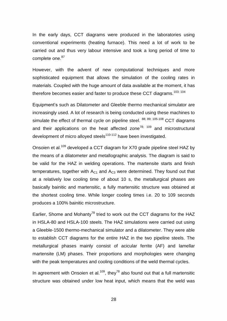
28

In the early days, CCT diagrams were produced in the laboratories using

conventional experiments (heating furnace). This need a lot of work to be

carried out and thus very labour intensive and took a long period of time to

complete one.87

However, with the advent of new computational techniques and more

sophisticated equipment that allows the simulation of the cooling rates in

materials. Coupled with the huge amount of data available at the moment, it has

therefore becomes easier and faster to produce these CCT diagrams.103; 104

Equipment’s such as Dilatometer and Gleeble thermo mechanical simulator are

increasingly used. A lot of research is being conducted using these machines to

simulate the effect of thermal cycle on pipeline steel. 88; 89; 105-108 CCT diagrams

and their applications on the heat affected zone78; 109 and microstructural

development of micro alloyed steels110-112 have been investigated.

Onsoien et al.109 developed a CCT diagram for X70 grade pipeline steel HAZ by

the means of a dilatometer and metallographic analysis. The diagram is said to

be valid for the HAZ in welding operations. The martensite starts and finish

temperatures, together with AC1 and AC3 were determined. They found out that

at a relatively low cooling time of about 10 s, the metallurgical phases are

basically bainitic and martensitic, a fully martensitic structure was obtained at

the shortest cooling time. While longer cooling times i.e. 20 to 109 seconds

produces a 100% bainitic microstructure.

Earlier, Shome and Mohanty78 tried to work out the CCT diagrams for the HAZ

in HSLA-80 and HSLA-100 steels. The HAZ simulations were carried out using

a Gleeble-1500 thermo-mechanical simulator and a dilatometer. They were able

to establish CCT diagrams for the entire HAZ in the two pipeline steels. The

metallurgical phases mainly consist of acicular ferrite (AF) and lamellar

martensite (LM) phases. Their proportions and morphologies were changing

with the peak temperatures and cooling conditions of the weld thermal cycles.

In agreement with Onsoien et al.109, they78 also found out that a full martensitic

structure was obtained under low heat input, which means that the weld was

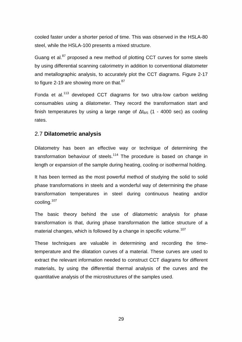
29

cooled faster under a shorter period of time. This was observed in the HSLA-80

steel, while the HSLA-100 presents a mixed structure.

Guang et al.87 proposed a new method of plotting CCT curves for some steels

by using differential scanning calorimetry in addition to conventional dilatometer

and metallographic analysis, to accurately plot the CCT diagrams. Figure 2-17

to figure 2-19 are showing more on that.87

Fonda et al.113 developed CCT diagrams for two ultra-low carbon welding

consumables using a dilatometer. They record the transformation start and

finish temperatures by using a large range of Δt8/5 (1 - 4000 sec) as cooling

rates.

Dilatometric analysis 2.7

Dilatometry has been an effective way or technique of determining the

transformation behaviour of steels.114 The procedure is based on change in

length or expansion of the sample during heating, cooling or isothermal holding.

It has been termed as the most powerful method of studying the solid to solid

phase transformations in steels and a wonderful way of determining the phase

transformation temperatures in steel during continuous heating and/or

cooling.107

The basic theory behind the use of dilatometric analysis for phase

transformation is that, during phase transformation the lattice structure of a

material changes, which is followed by a change in specific volume.107

These techniques are valuable in determining and recording the time-

temperature and the dilatation curves of a material. These curves are used to

extract the relevant information needed to construct CCT diagrams for different

materials, by using the differential thermal analysis of the curves and the

quantitative analysis of the microstructures of the samples used.

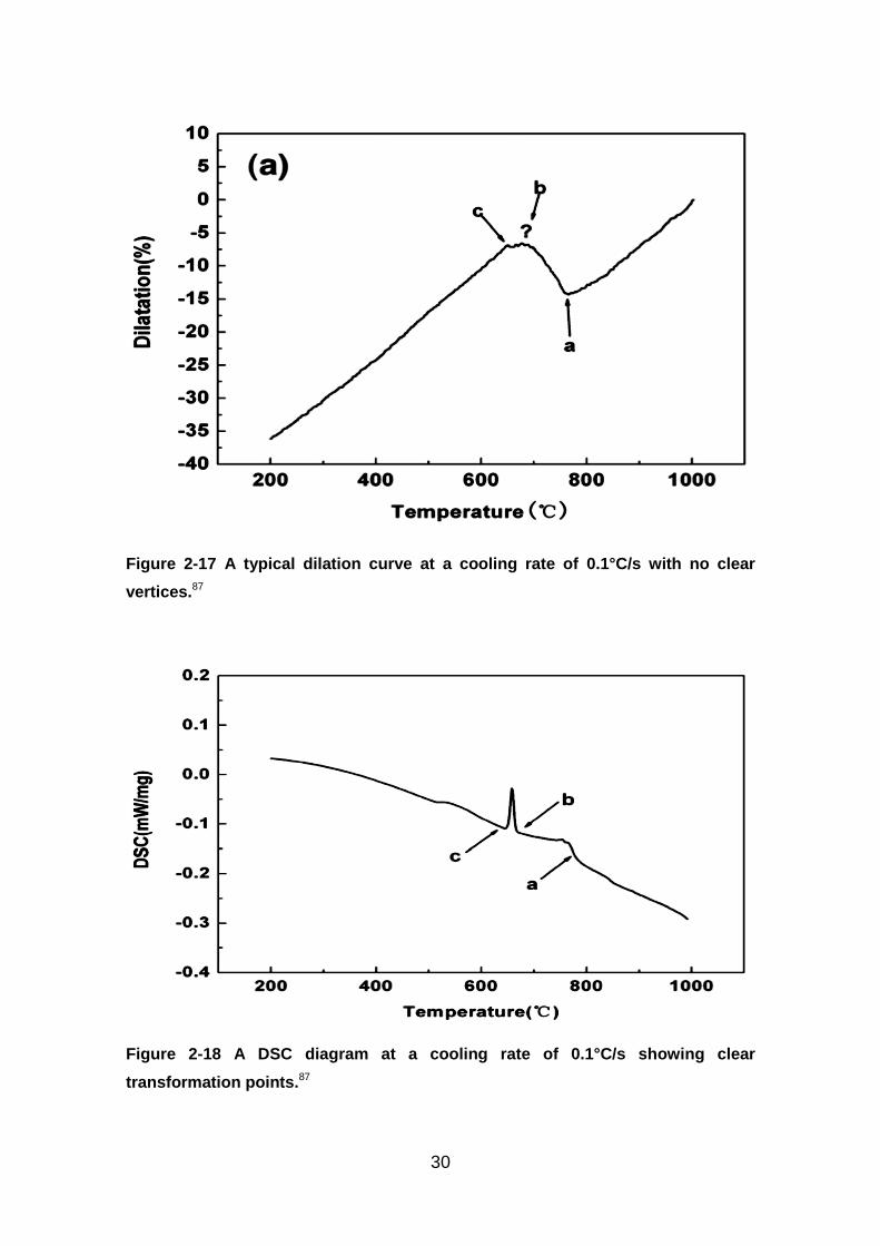
30

Figure 2-17 A typical dilation curve at a cooling rate of 0.1°C/s with no clear

vertices.87

Figure 2-18 A DSC diagram at a cooling rate of 0.1°C/s showing clear

transformation points.87

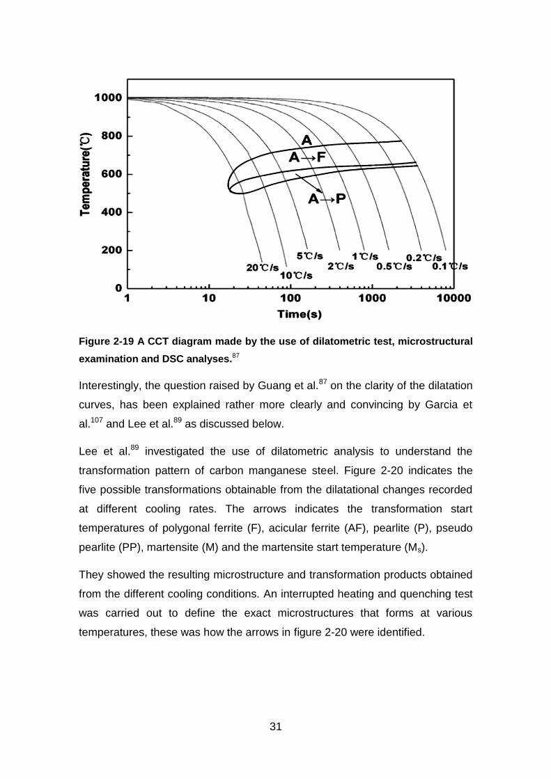
31

Figure 2-19 A CCT diagram made by the use of dilatometric test, microstructural

examination and DSC analyses.87

Interestingly, the question raised by Guang et al.87 on the clarity of the dilatation

curves, has been explained rather more clearly and convincing by Garcia et

al.107 and Lee et al.89 as discussed below.

Lee et al.89 investigated the use of dilatometric analysis to understand the

transformation pattern of carbon manganese steel. Figure 2-20 indicates the

five possible transformations obtainable from the dilatational changes recorded

at different cooling rates. The arrows indicates the transformation start

temperatures of polygonal ferrite (F), acicular ferrite (AF), pearlite (P), pseudo

pearlite (PP), martensite (M) and the martensite start temperature (Ms).

They showed the resulting microstructure and transformation products obtained

from the different cooling conditions. An interrupted heating and quenching test

was carried out to define the exact microstructures that forms at various

temperatures, these was how the arrows in figure 2-20 were identified.

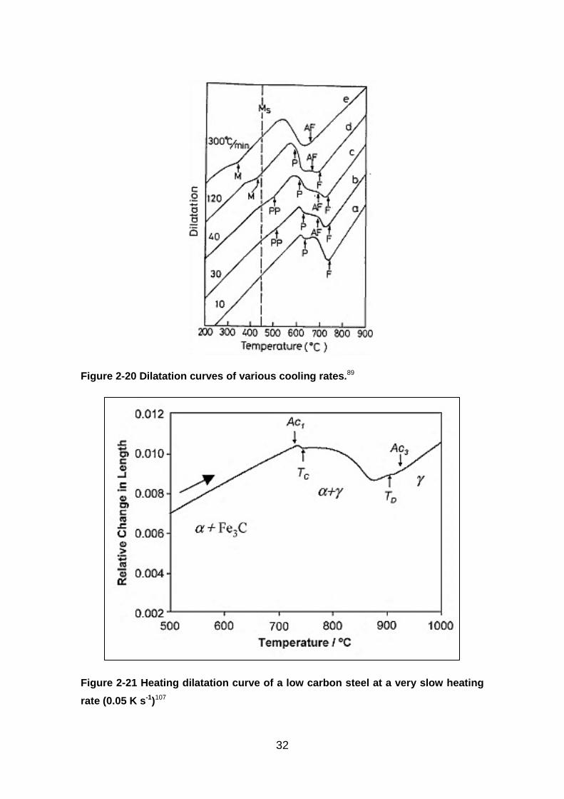
32

Figure 2-20 Dilatation curves of various cooling rates.89

Figure 2-21 Heating dilatation curve of a low carbon steel at a very slow heating

rate (0.05 K s-1)107

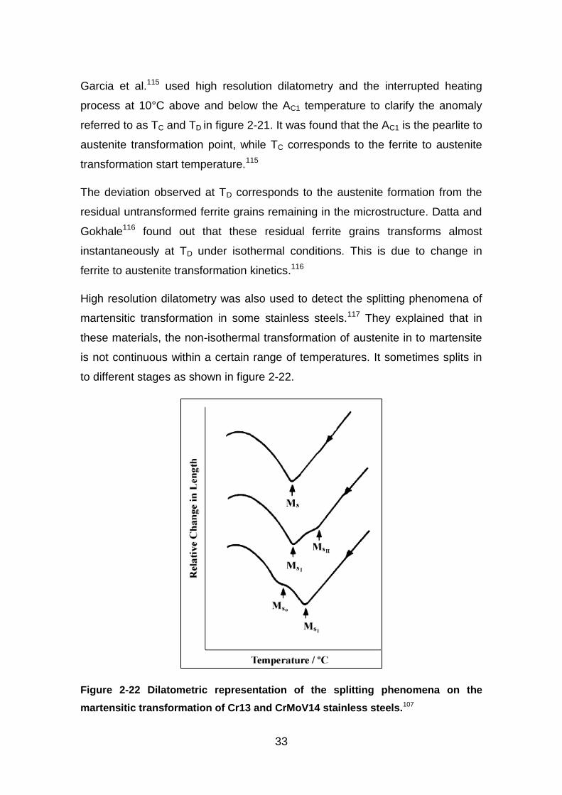
33

Garcia et al.115 used high resolution dilatometry and the interrupted heating

process at 10°C above and below the AC1 temperature to clarify the anomaly

referred to as TC and TD in figure 2-21. It was found that the AC1 is the pearlite to

austenite transformation point, while TC corresponds to the ferrite to austenite

transformation start temperature.115

The deviation observed at TD corresponds to the austenite formation from the

residual untransformed ferrite grains remaining in the microstructure. Datta and

Gokhale116 found out that these residual ferrite grains transforms almost

instantaneously at TD under isothermal conditions. This is due to change in

ferrite to austenite transformation kinetics.116

High resolution dilatometry was also used to detect the splitting phenomena of

martensitic transformation in some stainless steels.117 They explained that in

these materials, the non-isothermal transformation of austenite in to martensite

is not continuous within a certain range of temperatures. It sometimes splits in

to different stages as shown in figure 2-22.

Figure 2-22 Dilatometric representation of the splitting phenomena on the

martensitic transformation of Cr13 and CrMoV14 stainless steels.107

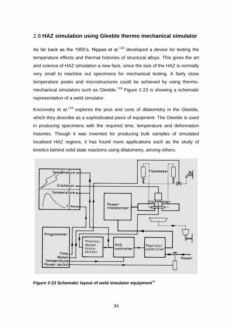
34

HAZ simulation using Gleeble thermo mechanical simulator 2.8

As far back as the 1950’s, Nippes et al.118 developed a device for testing the

temperature effects and thermal histories of structural alloys. This gives the art

and science of HAZ simulation a new face, since the size of the HAZ is normally

very small to machine out specimens for mechanical testing. A fairly close

temperature peaks and microstructures could be achieved by using thermo-

mechanical simulators such as Gleeble.119 Figure 2-23 is showing a schematic

representation of a weld simulator.

Knorovsky et al.119 explores the pros and cons of dilatometry in the Gleeble,

which they describe as a sophisticated piece of equipment. The Gleeble is used

in producing specimens with the required time, temperature and deformation

histories. Though it was invented for producing bulk samples of simulated

localised HAZ regions, it has found more applications such as the study of

kinetics behind solid state reactions using dilatometry, among others.

Figure 2-23 Schematic layout of weld simulator equipment49

35

They119 also outlined the common errors as bad laboratory practice, inadequate

personnel training and equipment condition (i.e. calibration, functionality and

general maintenance). The non-uniformity generally occurring in the material

and thermal distribution within the samples are other areas of concern.

2.8.1 Modelling of weld simulation

Models have been developed to simulate the thermal cycles, cooling rates and

phase transformation in both weld metal and HAZ, using various welding

processes such as GMAW tandem and dual tandem processes. These models

were developed to predict the mechanical properties of girth welds on pipelines

steels.120

Garcia et al.121 modelled the pearlite-to-austenite transformation in eutectoid

steel. They apply a mathematical model using the Avrami equation, which

successfully reproduce the kinetics involved in pearlite-to-austenite

transformation, during continuous heating. The Experimental transformation

temperatures AC1 and AC3, and the overall dilatometric behaviour due to

austenite formation were in good agreement with their predicted results. On the

other hand, austenite to ferrite phase transformation in low alloy steels was also

investigated by Gamsjager et al.122

Other researchers123-125 have also looked at the phase transformation kinetics in

relation to dilatation curves and the isothermal decomposition of austenite.

Effect of different welding procedures on HAZ toughness 2.9

The use of modern efficient and highly productive welding procedures has

become inevitable for the pipeline construction companies. High strength and

toughness is essential in both girth weld metal and the neighbouring heat

affected zones (HAZ). Especially in the application of strain based design, the

requirements for strength and toughness is becoming more stringent.126

Hamad et al.127 have looked at the effect of different GMAW procedures,

including dual, single and tandem torches on the HAZ toughness of X80 grade.

36

They use both crack tip opening displacement (CTOD) and Charpy impact test

to evaluate the HAZ toughness. Finally they conclude that lower heat input

coupled with lower t8/5 cooling times results in a considerable improvement of

the CTOD values.

Effect of composition 2.10

It has been established128; 129 long ago that chemical composition130 determines

the martensitic substructure, by influencing the Ms temperature and the strength

of the martensite formed. Due to the role of most alloying elements as solid

solution strengtheners in austenite, the thermodynamic driving force for initiating

martensitic shear transformation is increased, while the Ms temperature is

lowered.58

The results of McMahon and Thomas58 showed thin sheets of highly deformed

retained austenite surrounding some of the martensite laths in all the as-

quenched samples. Upon heating to a tempering temperature of about 200ºC,

the interlath austenite was reduced, while upon tempering at 400ºC, the

interlath disappears completely. This indicates that the tempering process has

transformed the retained austenite into ferrite, followed by precipitation of

interlath carbides, this leads to a loss in toughness.

The influence of niobium on the microstructure, mechanical properties and the

transformation kinetics of the coarse grain heat affected zone (CGHAZ), in high

strength low alloy steels (HSLA) using different heat inputs has been

investigated.131

Their results showed that the addition of 0.026% niobium decreased the

transformation start temperature of the steel by about 15°C to 30°C, when

compared with steel without niobium. They also showed that 0.026% niobium

addition can lead to a very significant deterioration of CGHAZ toughness, when

welded at high heat inputs. This was related to the formation of substantial

amount of granular bainite. But at low heat inputs the toughness decreases a

little.

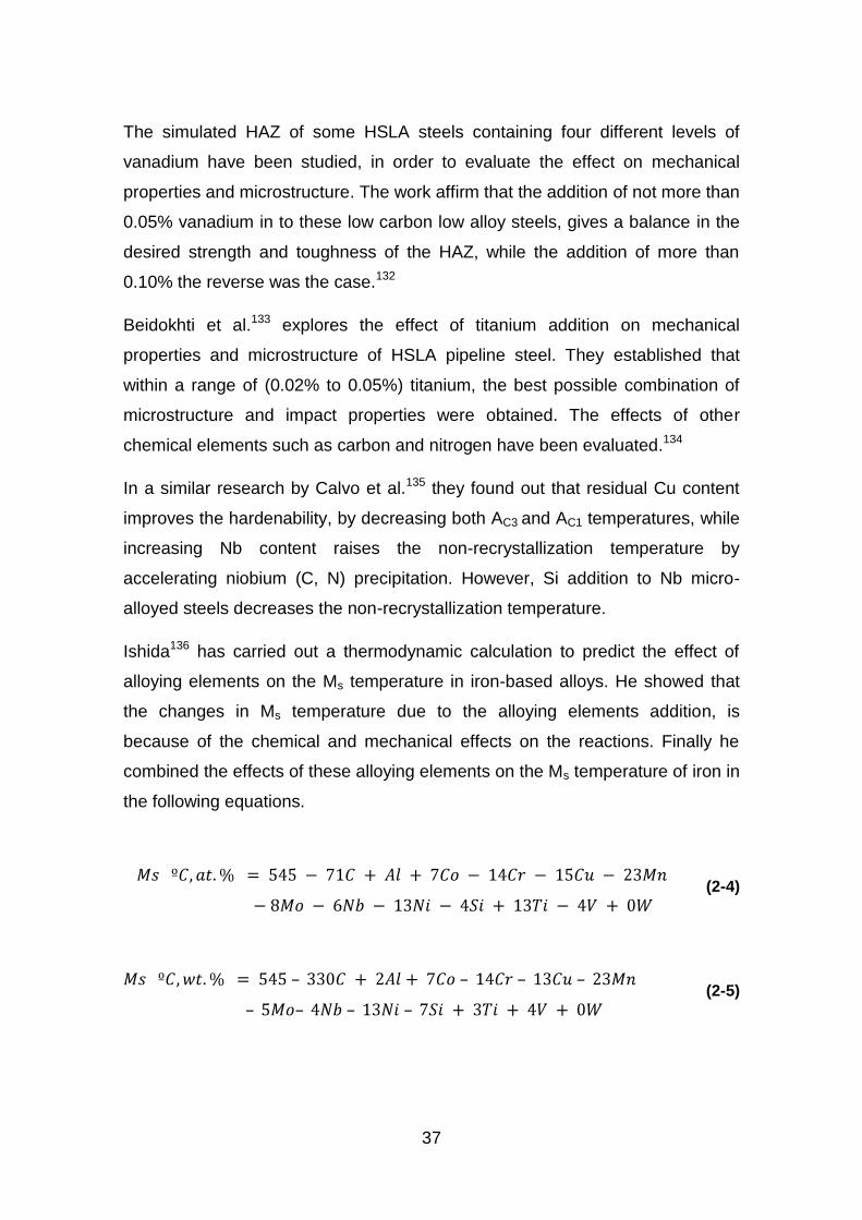
37

The simulated HAZ of some HSLA steels containing four different levels of

vanadium have been studied, in order to evaluate the effect on mechanical

properties and microstructure. The work affirm that the addition of not more than

0.05% vanadium in to these low carbon low alloy steels, gives a balance in the

desired strength and toughness of the HAZ, while the addition of more than

0.10% the reverse was the case.132

Beidokhti et al.133 explores the effect of titanium addition on mechanical

properties and microstructure of HSLA pipeline steel. They established that

within a range of (0.02% to 0.05%) titanium, the best possible combination of

microstructure and impact properties were obtained. The effects of other

chemical elements such as carbon and nitrogen have been evaluated.134

In a similar research by Calvo et al.135 they found out that residual Cu content

improves the hardenability, by decreasing both AC3 and AC1 temperatures, while

increasing Nb content raises the non-recrystallization temperature by

accelerating niobium (C, N) precipitation. However, Si addition to Nb micro-

alloyed steels decreases the non-recrystallization temperature.

Ishida136 has carried out a thermodynamic calculation to predict the effect of

alloying elements on the Ms temperature in iron-based alloys. He showed that

the changes in Ms temperature due to the alloying elements addition, is

because of the chemical and mechanical effects on the reactions. Finally he

combined the effects of these alloying elements on the Ms temperature of iron in

the following equations.

(2-4)

(2-5)

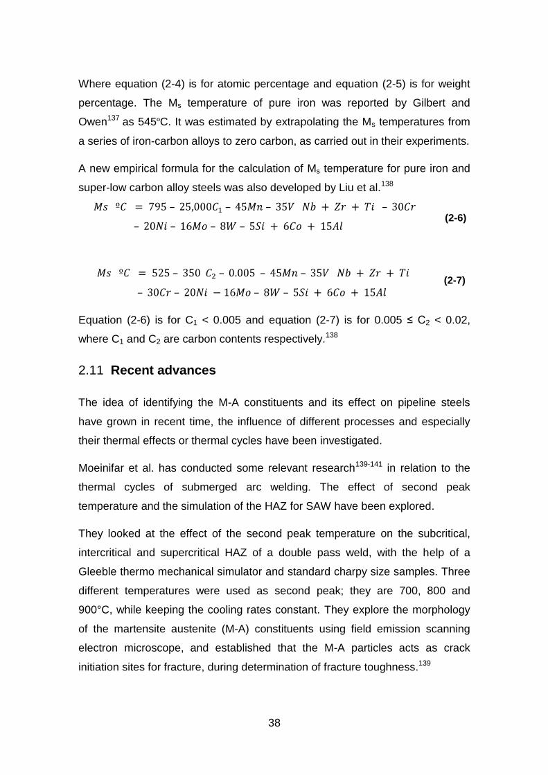
38

Where equation (2-4) is for atomic percentage and equation (2-5) is for weight

percentage. The Ms temperature of pure iron was reported by Gilbert and

Owen137 as 545ºC. It was estimated by extrapolating the Ms temperatures from

a series of iron-carbon alloys to zero carbon, as carried out in their experiments.

A new empirical formula for the calculation of Ms temperature for pure iron and

super-low carbon alloy steels was also developed by Liu et al.138

(2-6)

(2-7)

Equation (2-6) is for C1 < 0.005 and equation (2-7) is for 0.005 ≤ C2 < 0.02,

where C1 and C2 are carbon contents respectively.138

Recent advances 2.11

The idea of identifying the M-A constituents and its effect on pipeline steels

have grown in recent time, the influence of different processes and especially

their thermal effects or thermal cycles have been investigated.

Moeinifar et al. has conducted some relevant research139-141 in relation to the

thermal cycles of submerged arc welding. The effect of second peak

temperature and the simulation of the HAZ for SAW have been explored.

They looked at the effect of the second peak temperature on the subcritical,

intercritical and supercritical HAZ of a double pass weld, with the help of a

Gleeble thermo mechanical simulator and standard charpy size samples. Three

different temperatures were used as second peak; they are 700, 800 and

900°C, while keeping the cooling rates constant. They explore the morphology

of the martensite austenite (M-A) constituents using field emission scanning

electron microscope, and established that the M-A particles acts as crack

initiation sites for fracture, during determination of fracture toughness.139

39

Influence of thermal cycles on the properties of CGHAZ has been examined, it

was established that increase in hardness of the CGHAZ was because of the

fractional area of the M-A particles due to different cooling rates.140

Suzuki et al.142 made use of oversize charpy samples (11 × 11 mm) for thermal

simulation to check the influence of M-A islands on HAZ fracture due to high

heat input. The calculated and simulated thermal cycles used in their research

indicated that, the higher the heat input the longer it takes to reach the peak

temperature, this is far from the reality of a real weld thermal cycle, because in

a real weld, the heating is very fast.

It might be more logical to infer that during welding with a higher heat input the

heating will be more rapid when compared to lower heat input, where the rise in

temperature is less rapid.142

In another research conducted by Zhang et al.131 by using similar sample size

as used by Suzuki et al.142 very fast heating rate (500 °C/sec) was used. This

was a similar heating rate observed in a real weld, but a holding time of 3

seconds was used. This was not the case when compared to a real weld

thermal cycle.

Li et al. 143 also use oversized charpy samples (10.5 × 10.5 × 80 mm) to

thermally simulate the CGHAZ of X70 grade pipeline steel welds, made by

manual metal arc welding with a heat input of 1.2 kJ/mm. They use a heating

rate of 200 °C/sec and a peak temperature of 1350°C, they also hold at the

peak temperature for 1.2 seconds.

Summary 2.12

This literature review has critically looked in to the formation of local brittle

zones in the heat affected zone of a multi-pass weld. The theories behind the

formation of the M-A constituents and the techniques used in order to identify

the M-A phase was also reviewed. The inter-relationship between phase

transformation, inter-pass temperature and continuous cooling of a multi-pass

weld and their influence on formation of M-A phase was also discussed.

40

Techniques such as dilatometric analysis, heat affected zone simulation,

different etching techniques, optical and scanning electron microscopy

techniques has also been reviewed.

A substantial amount of research have gone in to identifying and characterizing

the M-A phase, which has been linked to the formation of local brittle zones.

There is a good understanding of the M-A phase formation in general and

especially on multi-pass welds, the theories supporting it are quite elaborate. A

good number of techniques have been developed for this purpose, but there is

no certainty in the mode of formation of the local brittle zones in a real weld, in

terms of phase transformation kinetics.

There is no comprehensive understanding of the thermal cycles responsible for

the formation of these brittle phases in a real weld. Most of the researches were

making some reasonable extrapolations of the simulated results on to the real

welds.

On the other hand, simulation of the various heat affected zones on charpy

impact samples in order characterize the effect of the various thermal cycles on

the HAZ toughness have been extensively researched. However, the thermal

cycles used in terms of heating and cooling are significantly different from a real

weld situation. Most of the researchers generate their simulated thermal cycles

from computer simulation and welding software.

In this research CCT diagrams were constructed using dilatometric analysis

techniques. Understanding welding thermal cycles through instrumented welds,

leads to precise knowledge of phase transformation products from the

constructed CCT diagrams.

It was shown that combining all these aspects of research would lead to the

understanding of M-A phase formation in real life multi-pass weld.

41

3 AIMS AND OBJECTIVES

Aim 3.1

The aim of this research is to develop fundamental understanding on the

underpinning process factors that lead to the formation of brittle phases in the

heat affected zones (HAZ) of multi-pass pipeline steels welds.

The research will try to derive a simpler methodology to characterise the effect

of multiple thermal cycle on the toughness of the high strength low alloy pipeline

steels. Derivation of CCT diagrams of the same steels composition would aid in

understanding the metallurgical phase formation in the HAZ.

Therefore, a correlation between the metallurgical phase formation and

toughness characteristics can be drawn for different multiple thermal cycles

representing different welding processes.

Specific research objectives 3.2

This research has been narrowed down to four pipeline steels some of which

are susceptible to LBZ formation. The following are the research objectives:

1. To record the real HAZ thermal cycles from submerged arc and tandem

MIG welds.

2. Carry out CTOD testing of the welds HAZ to check the presence of LBZ.

3. Simulate those thermal cycles in a thermo-mechanical simulator (Gleeble

Machine) using standard charpy samples.

4. Impact toughness determination of the thermally simulated specimens.

5. Mechanical and metallurgical characterisation of the welds mentioned in

bullet 1 above and the thermal simulation samples mentioned in bullet 3.

6. Identify the thermal cycles which lead to the formation of brittle

metallurgical phases resulting in loss of toughness.

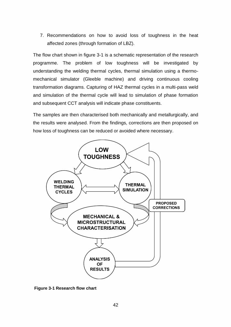
42

7. Recommendations on how to avoid loss of toughness in the heat

affected zones (through formation of LBZ).

The flow chart shown in figure 3-1 is a schematic representation of the research

programme. The problem of low toughness will be investigated by

understanding the welding thermal cycles, thermal simulation using a thermo-

mechanical simulator (Gleeble machine) and driving continuous cooling

transformation diagrams. Capturing of HAZ thermal cycles in a multi-pass weld

and simulation of the thermal cycle will lead to simulation of phase formation

and subsequent CCT analysis will indicate phase constituents.

The samples are then characterised both mechanically and metallurgically, and

the results were analysed. From the findings, corrections are then proposed on

how loss of toughness can be reduced or avoided where necessary.

Figure 3-1 Research flow chart

43

4 MATERIALS AND EQUIPMENTS

The materials used in this work are presented in this chapter. They comprise of

pipeline steels and consumables among others. Equipments used for welding

processes, weld instrumentation, thermal simulation and characterisation

(metallurgical and mechanical) are also presented.

Each of the above mentioned categories is presented as an independent

heading below. Only the most important materials and instruments used are

presented and discussed.

Materials 4.1

4.1.1 Pipeline steels

Three different grades of high-strength pipeline steels were used in this project.

They were X65, X70 and X100 grades, the chemical compositions are given in

table 4-1.

The X65 (a) is a seamless pipe, while the X65 (b) is a thermo-mechanically

controlled processed (TMCP) material, both materials have specified minimum

yield strength of 450 MPa.98; 144

The X70 and X100 pipes are thermo-mechanically controlled processed

(TMCP) materials. They both have specified minimum yield strengths of 485

MPa and 690 MPa respectively.98; 144 The outside diameters and wall

thicknesses of all the steel grades are given in table 4-1.

DNV-OS-F101 recommends that for pipes with carbon content ≤ 0.12%, the

carbon equivalent should be calculated using the Pcm formula, while for carbon

content > 0.12% the CE formula should be used.144

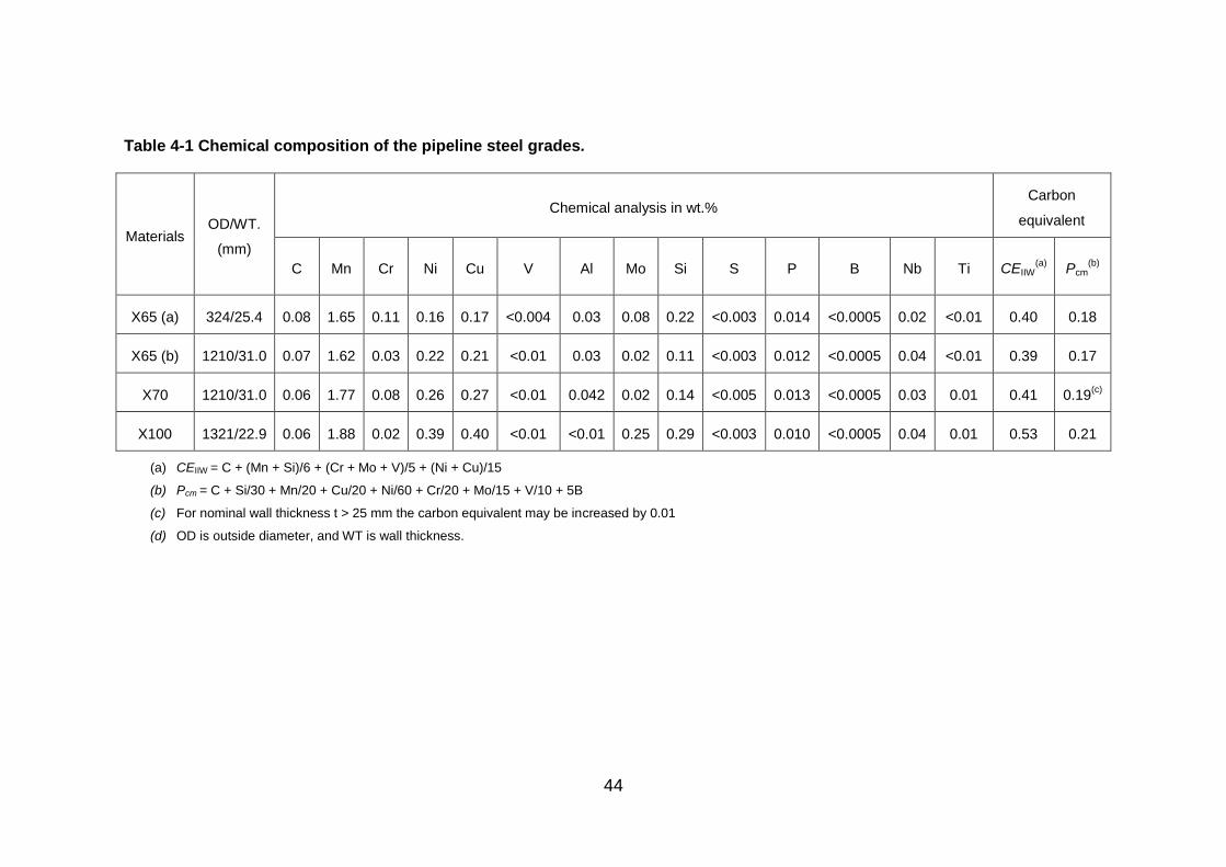
44

Table 4-1 Chemical composition of the pipeline steel grades.

Materials OD/WT.

(mm)

Chemical analysis in wt.% Carbon

equivalent

C Mn Cr Ni Cu V Al Mo Si S P B Nb Ti CEIIW(a)

Pcm(b)

X65 (a) 324/25.4 0.08 1.65 0.11 0.16 0.17 <0.004 0.03 0.08 0.22 <0.003 0.014 <0.0005 0.02 <0.01 0.40 0.18

X65 (b) 1210/31.0 0.07 1.62 0.03 0.22 0.21 <0.01 0.03 0.02 0.11 <0.003 0.012 <0.0005 0.04 <0.01 0.39 0.17

X70 1210/31.0 0.06 1.77 0.08 0.26 0.27 <0.01 0.042 0.02 0.14 <0.005 0.013 <0.0005 0.03 0.01 0.41 0.19(c)

X100 1321/22.9 0.06 1.88 0.02 0.39 0.40 <0.01 <0.01 0.25 0.29 <0.003 0.010 <0.0005 0.04 0.01 0.53 0.21

(a) CEIIW = C + (Mn + Si)/6 + (Cr + Mo + V)/5 + (Ni + Cu)/15

(b) Pcm = C + Si/30 + Mn/20 + Cu/20 + Ni/60 + Cr/20 + Mo/15 + V/10 + 5B

(c) For nominal wall thickness t > 25 mm the carbon equivalent may be increased by 0.01

(d) OD is outside diameter, and WT is wall thickness.

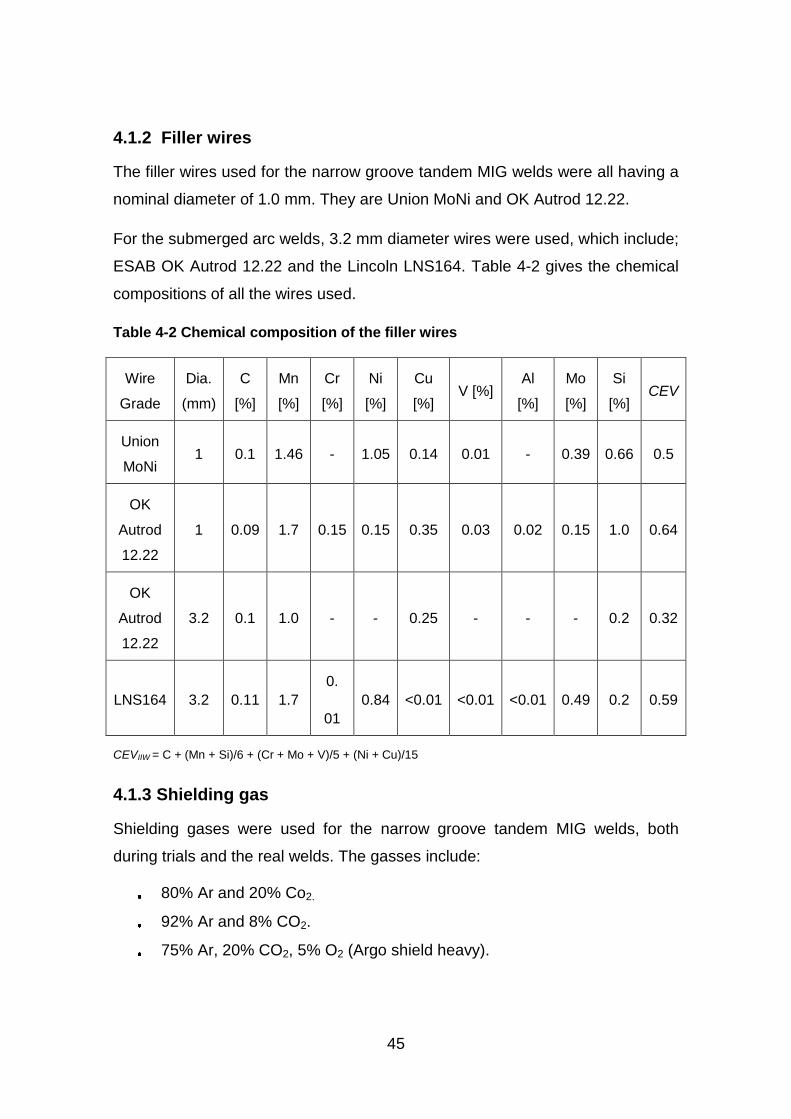
45

4.1.2 Filler wires

The filler wires used for the narrow groove tandem MIG welds were all having a

nominal diameter of 1.0 mm. They are Union MoNi and OK Autrod 12.22.

For the submerged arc welds, 3.2 mm diameter wires were used, which include;

ESAB OK Autrod 12.22 and the Lincoln LNS164. Table 4-2 gives the chemical

compositions of all the wires used.

Table 4-2 Chemical composition of the filler wires

Wire

Grade

Dia.

(mm)

C

[%]

Mn

[%]

Cr

[%]

Ni

[%]

Cu

[%] V [%]

Al

[%]

Mo

[%]

Si

[%] CEV

Union

MoNi 1 0.1 1.46 - 1.05 0.14 0.01 - 0.39 0.66 0.5

OK

Autrod

12.22

1 0.09 1.7 0.15 0.15 0.35 0.03 0.02 0.15 1.0 0.64

OK

Autrod

12.22

3.2 0.1 1.0 - - 0.25 - - - 0.2 0.32

LNS164 3.2 0.11 1.7

0.

01

0.84 <0.01 <0.01 <0.01 0.49 0.2 0.59

CEVIIW = C + (Mn + Si)/6 + (Cr + Mo + V)/5 + (Ni + Cu)/15

4.1.3 Shielding gas

Shielding gases were used for the narrow groove tandem MIG welds, both

during trials and the real welds. The gasses include:

80% Ar and 20% Co2.

92% Ar and 8% CO2.

75% Ar, 20% CO2, 5% O2 (Argo shield heavy).

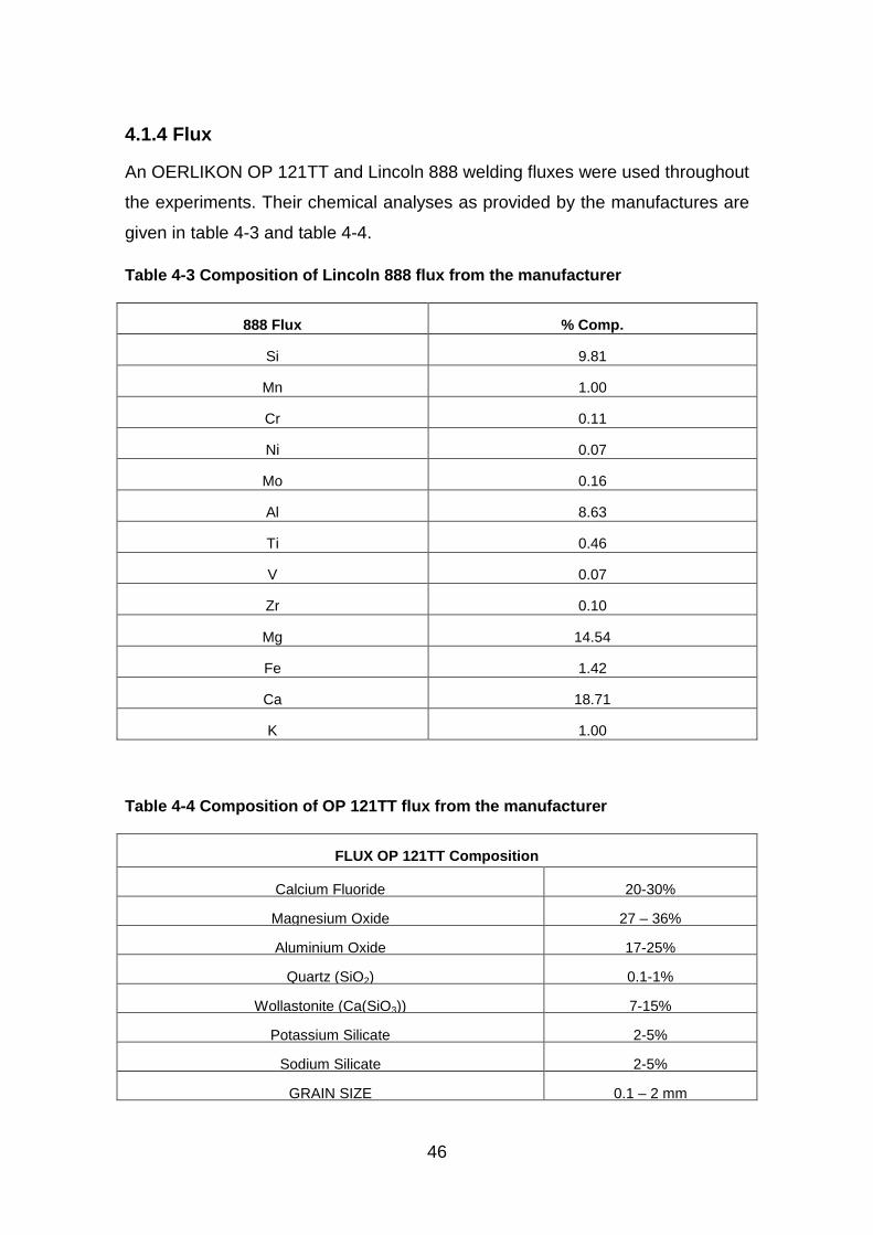
46

4.1.4 Flux

An OERLIKON OP 121TT and Lincoln 888 welding fluxes were used throughout

the experiments. Their chemical analyses as provided by the manufactures are

given in table 4-3 and table 4-4.

Table 4-3 Composition of Lincoln 888 flux from the manufacturer

888 Flux % Comp.

Si 9.81

Mn 1.00

Cr 0.11

Ni 0.07

Mo 0.16

Al 8.63

Ti 0.46

V 0.07

Zr 0.10

Mg 14.54

Fe 1.42

Ca 18.71

K 1.00

Table 4-4 Composition of OP 121TT flux from the manufacturer

FLUX OP 121TT Composition

Calcium Fluoride 20-30%

Magnesium Oxide 27 – 36%

Aluminium Oxide 17-25%

Quartz (SiO2) 0.1-1%

Wollastonite (Ca(SiO3)) 7-15%

Potassium Silicate 2-5%

Sodium Silicate 2-5%

GRAIN SIZE 0.1 – 2 mm

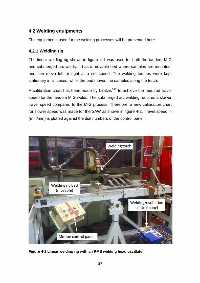
47

Welding equipments 4.2

The equipments used for the welding processes will be presented here.

4.2.1 Welding rig

The linear welding rig shown in figure 4-1 was used for both the tandem MIG

and submerged arc welds. It has a movable bed where samples are mounted,

and can move left or right at a set speed. The welding torches were kept

stationary in all cases, while the bed moves the samples along the torch.

A calibration chart has been made by Liratzis145 to achieve the required travel

speed for the tandem MIG welds. The submerged arc welding requires a slower

travel speed compared to the MIG process. Therefore, a new calibration chart

for slower speed was made for the SAW as shown in figure 4-2. Travel speed in

(mm/min) is plotted against the dial numbers of the control panel.

Figure 4-1 Linear welding rig with an RMS welding head oscillator

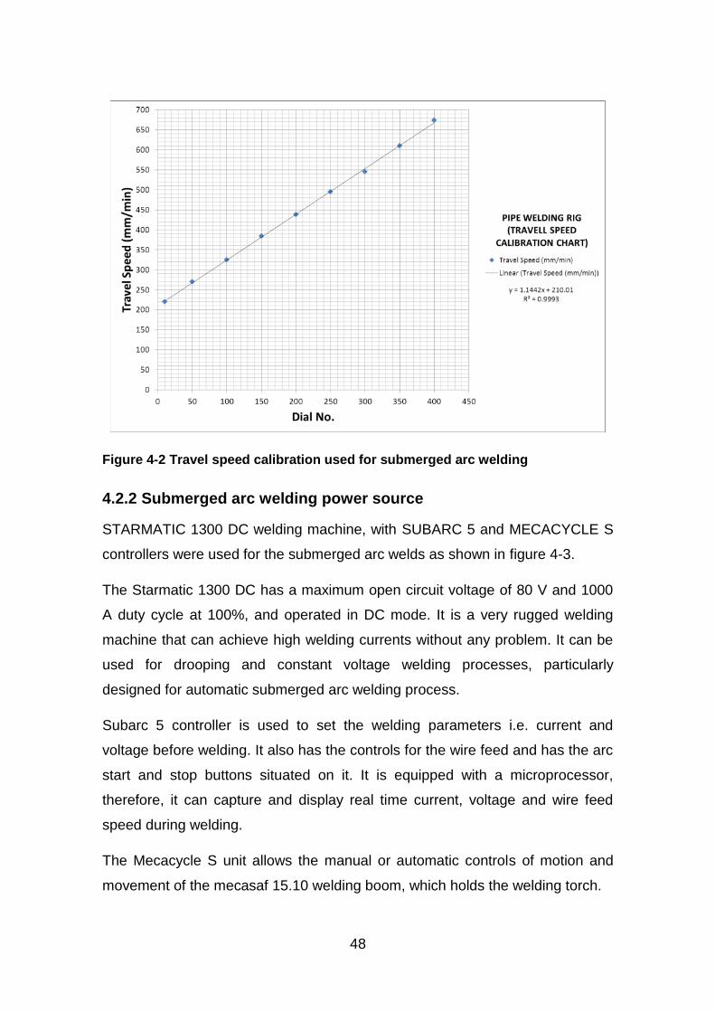
48

Figure 4-2 Travel speed calibration used for submerged arc welding

4.2.2 Submerged arc welding power source

STARMATIC 1300 DC welding machine, with SUBARC 5 and MECACYCLE S

controllers were used for the submerged arc welds as shown in figure 4-3.

The Starmatic 1300 DC has a maximum open circuit voltage of 80 V and 1000

A duty cycle at 100%, and operated in DC mode. It is a very rugged welding

machine that can achieve high welding currents without any problem. It can be

used for drooping and constant voltage welding processes, particularly

designed for automatic submerged arc welding process.

Subarc 5 controller is used to set the welding parameters i.e. current and

voltage before welding. It also has the controls for the wire feed and has the arc

start and stop buttons situated on it. It is equipped with a microprocessor,

therefore, it can capture and display real time current, voltage and wire feed

speed during welding.

The Mecacycle S unit allows the manual or automatic controls of motion and

movement of the mecasaf 15.10 welding boom, which holds the welding torch.

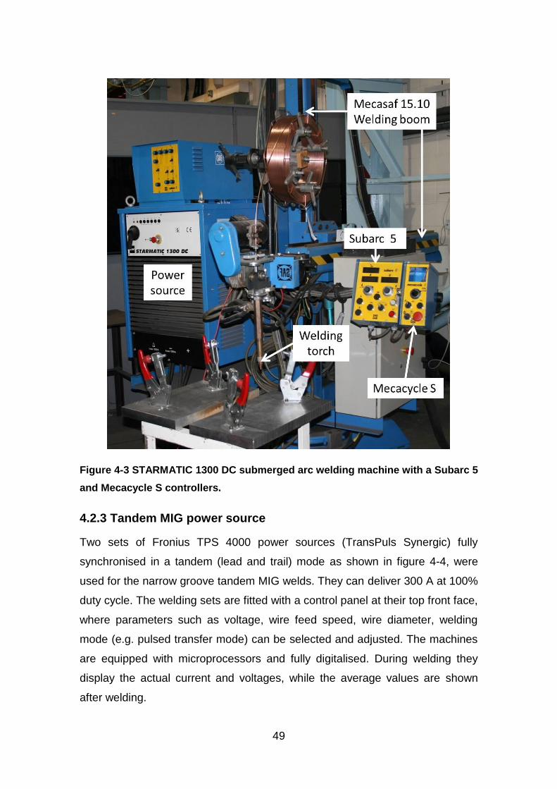
49

Figure 4-3 STARMATIC 1300 DC submerged arc welding machine with a Subarc 5

and Mecacycle S controllers.

4.2.3 Tandem MIG power source

Two sets of Fronius TPS 4000 power sources (TransPuls Synergic) fully

synchronised in a tandem (lead and trail) mode as shown in figure 4-4, were

used for the narrow groove tandem MIG welds. They can deliver 300 A at 100%

duty cycle. The welding sets are fitted with a control panel at their top front face,

where parameters such as voltage, wire feed speed, wire diameter, welding

mode (e.g. pulsed transfer mode) can be selected and adjusted. The machines

are equipped with microprocessors and fully digitalised. During welding they

display the actual current and voltages, while the average values are shown

after welding.

50

Figure 4-4 Fronius TPS 4000 thermo power welding machines

Weld Instrumentation 4.3

The instruments used in capturing the thermal cycles and the welding

parameters i.e. current, voltage and wire feed speed for the SAW and Narrow

groove tandem MIG welds are presented here.

4.3.1 Thermal cycles acquisition during welding processes

A data acquisition device was developed for the purpose of this research. This

was a modification to what Hudson146 built and used earlier at Cranfield

University. Standard office desktop computer and thermocouple data acquisition

device (NI PCIE-6351, X Series Multifunction DAQ) with a maximum frequency

of 100 MHz were used. They give the flexibility of capturing data at a very high

sampling rate. A SHC68-68-EPM Shielded cable was used to minimise the

noise. Figure 4-5 is a picture of the equipment. K-type (NiCr/Ni) thermocouples

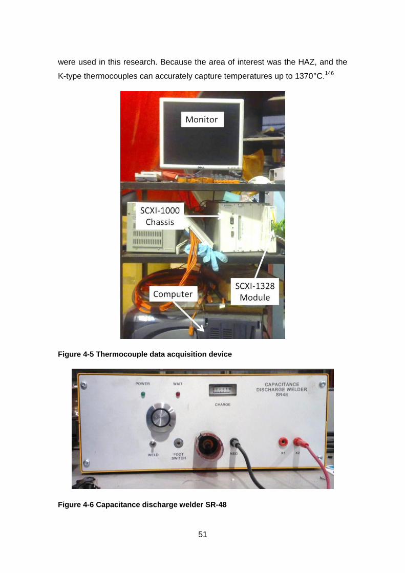
51

were used in this research. Because the area of interest was the HAZ, and the

K-type thermocouples can accurately capture temperatures up to 1370°C.146

Figure 4-5 Thermocouple data acquisition device

Figure 4-6 Capacitance discharge welder SR-48

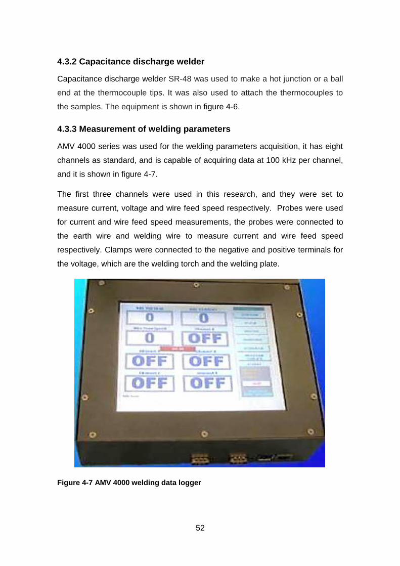
52

4.3.2 Capacitance discharge welder

Capacitance discharge welder SR-48 was used to make a hot junction or a ball

end at the thermocouple tips. It was also used to attach the thermocouples to

the samples. The equipment is shown in figure 4-6.

4.3.3 Measurement of welding parameters

AMV 4000 series was used for the welding parameters acquisition, it has eight

channels as standard, and is capable of acquiring data at 100 kHz per channel,

and it is shown in figure 4-7.

The first three channels were used in this research, and they were set to

measure current, voltage and wire feed speed respectively. Probes were used

for current and wire feed speed measurements, the probes were connected to

the earth wire and welding wire to measure current and wire feed speed

respectively. Clamps were connected to the negative and positive terminals for

the voltage, which are the welding torch and the welding plate.

Figure 4-7 AMV 4000 welding data logger

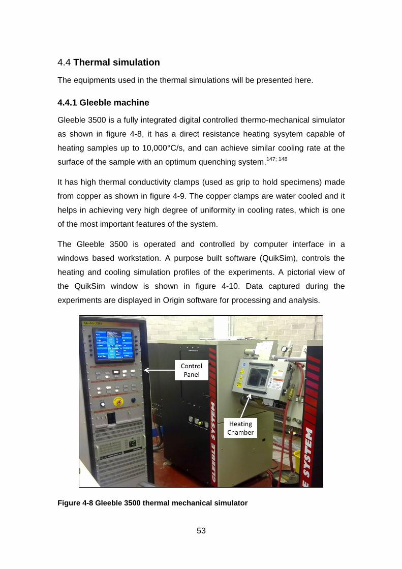
53

Thermal simulation 4.4

The equipments used in the thermal simulations will be presented here.

4.4.1 Gleeble machine

Gleeble 3500 is a fully integrated digital controlled thermo-mechanical simulator

as shown in figure 4-8, it has a direct resistance heating sysytem capable of

heating samples up to 10,000°C/s, and can achieve similar cooling rate at the

surface of the sample with an optimum quenching system.147; 148

It has high thermal conductivity clamps (used as grip to hold specimens) made

from copper as shown in figure 4-9. The copper clamps are water cooled and it

helps in achieving very high degree of uniformity in cooling rates, which is one

of the most important features of the system.

The Gleeble 3500 is operated and controlled by computer interface in a

windows based workstation. A purpose built software (QuikSim), controls the

heating and cooling simulation profiles of the experiments. A pictorial view of

the QuikSim window is shown in figure 4-10. Data captured during the

experiments are displayed in Origin software for processing and analysis.

Figure 4-8 Gleeble 3500 thermal mechanical simulator

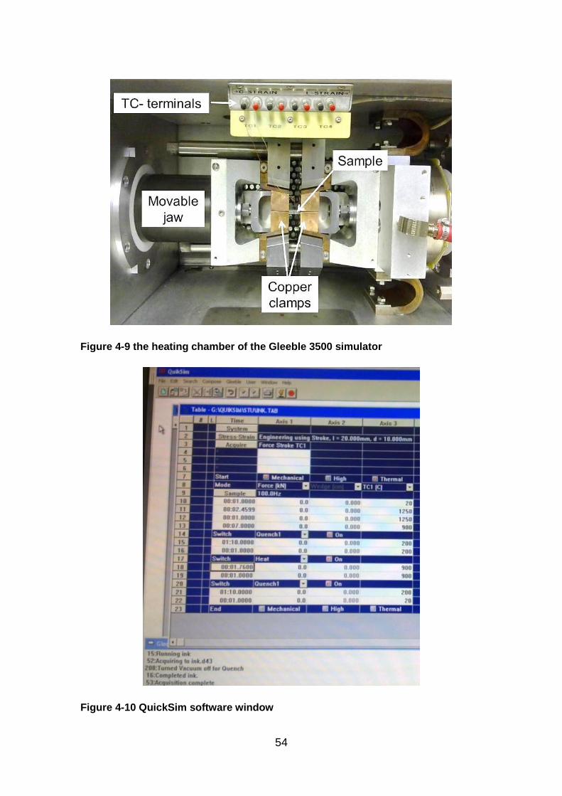
54

Figure 4-9 the heating chamber of the Gleeble 3500 simulator

Figure 4-10 QuickSim software window

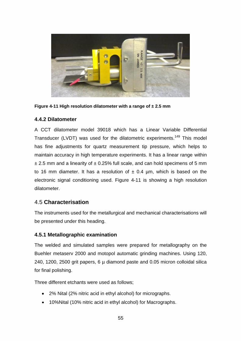
55

Figure 4-11 High resolution dilatometer with a range of ± 2.5 mm

4.4.2 Dilatometer

A CCT dilatometer model 39018 which has a Linear Variable Differential

Transducer (LVDT) was used for the dilatometric experiments.149 This model

has fine adjustments for quartz measurement tip pressure, which helps to

maintain accuracy in high temperature experiments. It has a linear range within

± 2.5 mm and a linearity of ± 0.25% full scale, and can hold specimens of 5 mm

to 16 mm diameter. It has a resolution of ± 0.4 µm, which is based on the

electronic signal conditioning used. Figure 4-11 is showing a high resolution

dilatometer.

Characterisation 4.5

The instruments used for the metallurgical and mechanical characterisations will

be presented under this heading.

4.5.1 Metallographic examination

The welded and simulated samples were prepared for metallography on the

Buehler metaserv 2000 and motopol automatic grinding machines. Using 120,

240, 1200, 2500 grit papers, 6 µ diamond paste and 0.05 micron colloidal silica

for final polishing.

Three different etchants were used as follows;

2% Nital (2% nitric acid in ethyl alcohol) for micrographs.

10%Nital (10% nitric acid in ethyl alcohol) for Macrographs.

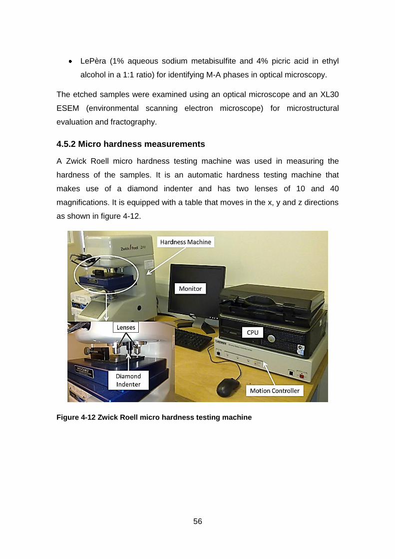
56

LePèra (1% aqueous sodium metabisulfite and 4% picric acid in ethyl

alcohol in a 1:1 ratio) for identifying M-A phases in optical microscopy.

The etched samples were examined using an optical microscope and an XL30

ESEM (environmental scanning electron microscope) for microstructural

evaluation and fractography.

4.5.2 Micro hardness measurements

A Zwick Roell micro hardness testing machine was used in measuring the

hardness of the samples. It is an automatic hardness testing machine that

makes use of a diamond indenter and has two lenses of 10 and 40

magnifications. It is equipped with a table that moves in the x, y and z directions

as shown in figure 4-12.

Figure 4-12 Zwick Roell micro hardness testing machine

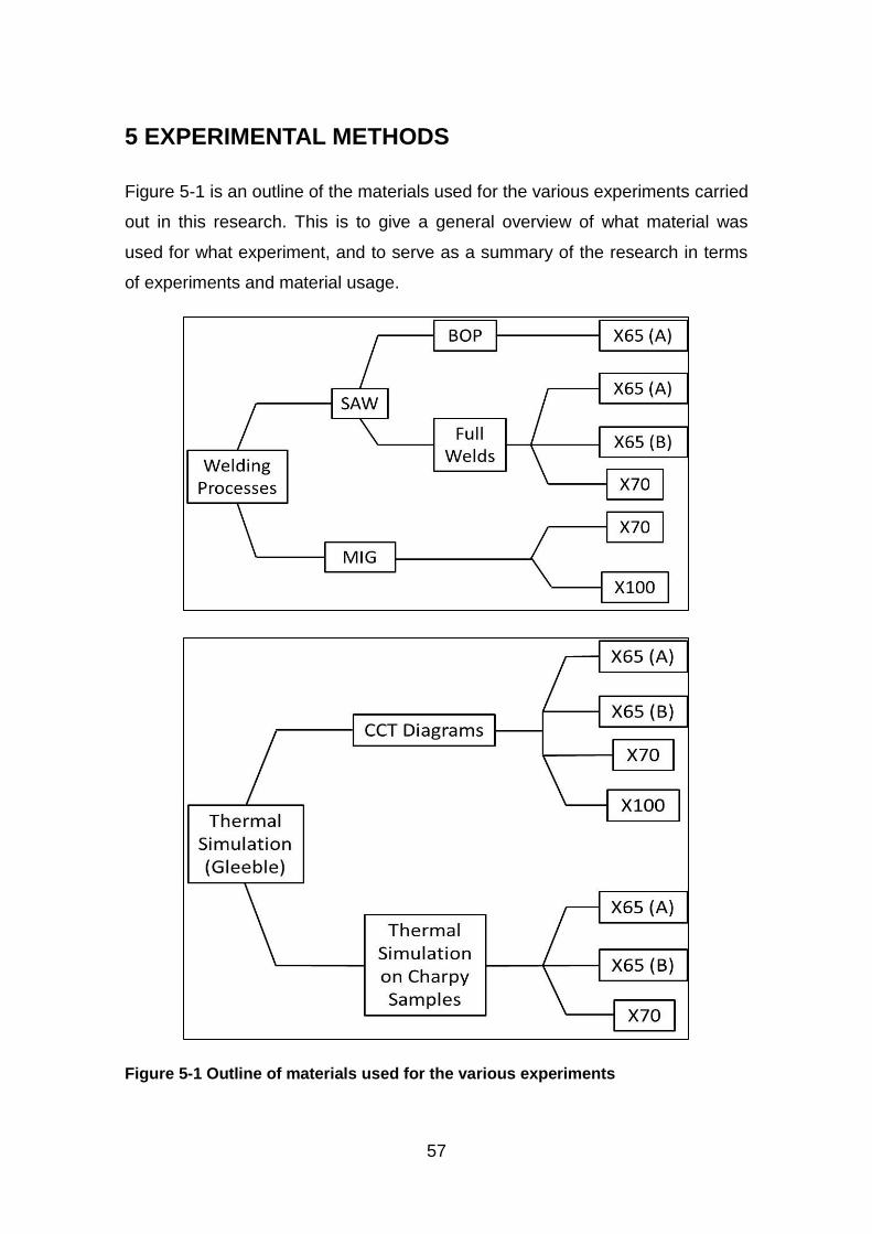
57

5 EXPERIMENTAL METHODS

Figure 5-1 is an outline of the materials used for the various experiments carried

out in this research. This is to give a general overview of what material was

used for what experiment, and to serve as a summary of the research in terms

of experiments and material usage.

Figure 5-1 Outline of materials used for the various experiments

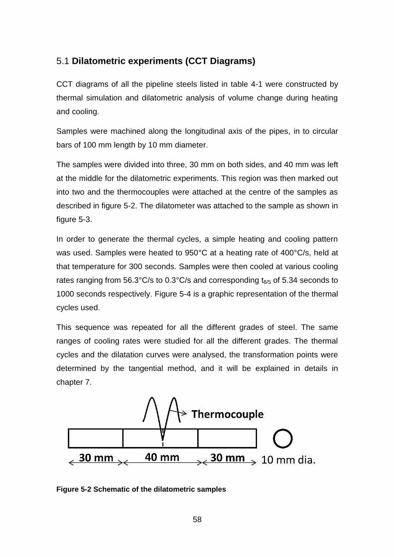
58

Dilatometric experiments (CCT Diagrams) 5.1

CCT diagrams of all the pipeline steels listed in table 4-1 were constructed by

thermal simulation and dilatometric analysis of volume change during heating

and cooling.

Samples were machined along the longitudinal axis of the pipes, in to circular

bars of 100 mm length by 10 mm diameter.

The samples were divided into three, 30 mm on both sides, and 40 mm was left

at the middle for the dilatometric experiments. This region was then marked out

into two and the thermocouples were attached at the centre of the samples as

described in figure 5-2. The dilatometer was attached to the sample as shown in

figure 5-3.

In order to generate the thermal cycles, a simple heating and cooling pattern

was used. Samples were heated to 950°C at a heating rate of 400°C/s, held at

that temperature for 300 seconds. Samples were then cooled at various cooling

rates ranging from 56.3°C/s to 0.3°C/s and corresponding t8/5 of 5.34 seconds to

1000 seconds respectively. Figure 5-4 is a graphic representation of the thermal

cycles used.

This sequence was repeated for all the different grades of steel. The same

ranges of cooling rates were studied for all the different grades. The thermal

cycles and the dilatation curves were analysed, the transformation points were

determined by the tangential method, and it will be explained in details in

chapter 7.

Figure 5-2 Schematic of the dilatometric samples

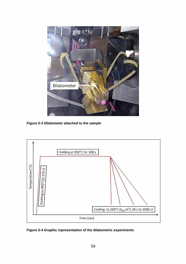
59

Figure 5-3 Dilatometer attached to the sample

Figure 5-4 Graphic representation of the dilatometric experiments

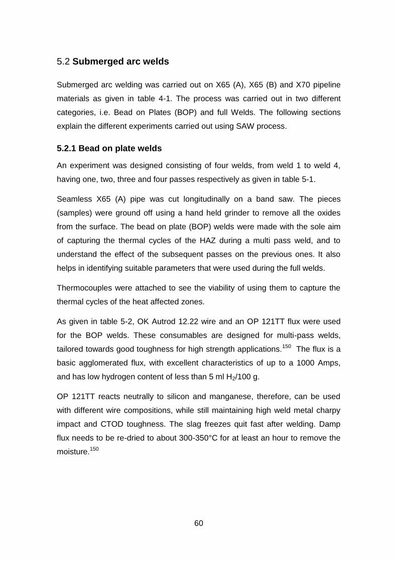
60

Submerged arc welds 5.2

Submerged arc welding was carried out on X65 (A), X65 (B) and X70 pipeline

materials as given in table 4-1. The process was carried out in two different

categories, i.e. Bead on Plates (BOP) and full Welds. The following sections

explain the different experiments carried out using SAW process.

5.2.1 Bead on plate welds

An experiment was designed consisting of four welds, from weld 1 to weld 4,

having one, two, three and four passes respectively as given in table 5-1.

Seamless X65 (A) pipe was cut longitudinally on a band saw. The pieces

(samples) were ground off using a hand held grinder to remove all the oxides

from the surface. The bead on plate (BOP) welds were made with the sole aim

of capturing the thermal cycles of the HAZ during a multi pass weld, and to

understand the effect of the subsequent passes on the previous ones. It also

helps in identifying suitable parameters that were used during the full welds.

Thermocouples were attached to see the viability of using them to capture the

thermal cycles of the heat affected zones.

As given in table 5-2, OK Autrod 12.22 wire and an OP 121TT flux were used

for the BOP welds. These consumables are designed for multi-pass welds,

tailored towards good toughness for high strength applications.150 The flux is a

basic agglomerated flux, with excellent characteristics of up to a 1000 Amps,

and has low hydrogen content of less than 5 ml H2/100 g.

OP 121TT reacts neutrally to silicon and manganese, therefore, can be used

with different wire compositions, while still maintaining high weld metal charpy

impact and CTOD toughness. The slag freezes quit fast after welding. Damp

flux needs to be re-dried to about 300-350°C for at least an hour to remove the

moisture.150

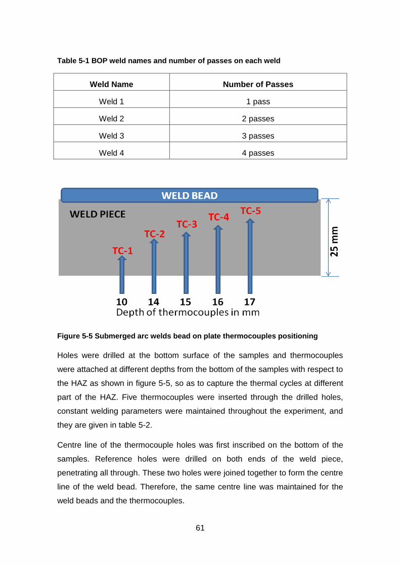
61

Table 5-1 BOP weld names and number of passes on each weld

Weld Name Number of Passes

Weld 1 1 pass

Weld 2 2 passes

Weld 3 3 passes

Weld 4 4 passes

Figure 5-5 Submerged arc welds bead on plate thermocouples positioning

Holes were drilled at the bottom surface of the samples and thermocouples

were attached at different depths from the bottom of the samples with respect to

the HAZ as shown in figure 5-5, so as to capture the thermal cycles at different

part of the HAZ. Five thermocouples were inserted through the drilled holes,

constant welding parameters were maintained throughout the experiment, and

they are given in table 5-2.

Centre line of the thermocouple holes was first inscribed on the bottom of the

samples. Reference holes were drilled on both ends of the weld piece,

penetrating all through. These two holes were joined together to form the centre

line of the weld bead. Therefore, the same centre line was maintained for the

weld beads and the thermocouples.

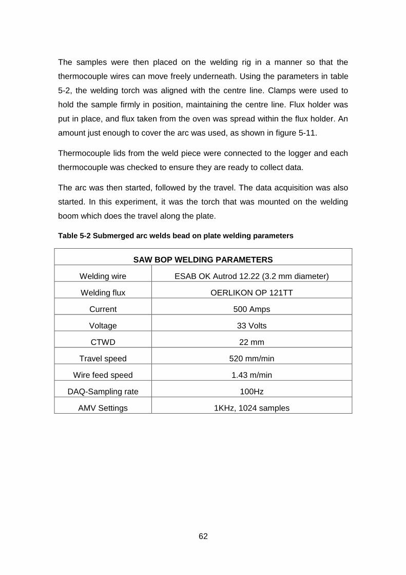
62

The samples were then placed on the welding rig in a manner so that the

thermocouple wires can move freely underneath. Using the parameters in table

5-2, the welding torch was aligned with the centre line. Clamps were used to

hold the sample firmly in position, maintaining the centre line. Flux holder was

put in place, and flux taken from the oven was spread within the flux holder. An

amount just enough to cover the arc was used, as shown in figure 5-11.

Thermocouple lids from the weld piece were connected to the logger and each

thermocouple was checked to ensure they are ready to collect data.

The arc was then started, followed by the travel. The data acquisition was also

started. In this experiment, it was the torch that was mounted on the welding

boom which does the travel along the plate.

Table 5-2 Submerged arc welds bead on plate welding parameters

SAW BOP WELDING PARAMETERS

Welding wire ESAB OK Autrod 12.22 (3.2 mm diameter)

Welding flux OERLIKON OP 121TT

Current 500 Amps

Voltage 33 Volts

CTWD 22 mm

Travel speed 520 mm/min

Wire feed speed 1.43 m/min

DAQ-Sampling rate 100Hz

AMV Settings 1KHz, 1024 samples

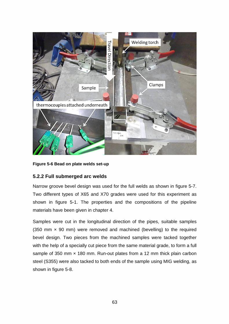
63

Figure 5-6 Bead on plate welds set-up

5.2.2 Full submerged arc welds

Narrow groove bevel design was used for the full welds as shown in figure 5-7.

Two different types of X65 and X70 grades were used for this experiment as

shown in figure 5-1. The properties and the compositions of the pipeline

materials have been given in chapter 4.

Samples were cut in the longitudinal direction of the pipes, suitable samples

(350 mm × 90 mm) were removed and machined (bevelling) to the required

bevel design. Two pieces from the machined samples were tacked together

with the help of a specially cut piece from the same material grade, to form a full

sample of 350 mm × 180 mm. Run-out plates from a 12 mm thick plain carbon

steel (S355) were also tacked to both ends of the sample using MIG welding, as

shown in figure 5-8.

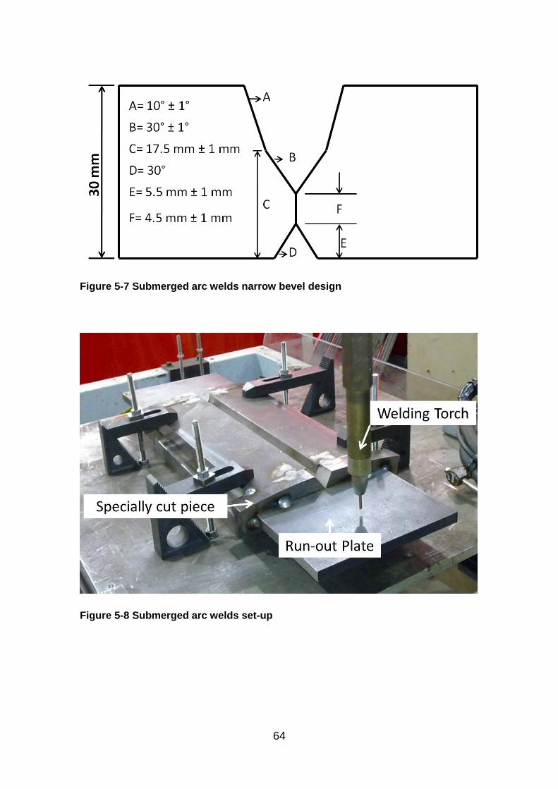
64

Figure 5-7 Submerged arc welds narrow bevel design

Figure 5-8 Submerged arc welds set-up

65

After been tacked together, the thermocouples holes were drilled on a milling

machine. The thermocouples were attached using a capacitance discharge

welder through the drilled holes.

Six thermocouples were used on each of the welds, two at a depth of 10 mm

from the bottom and four at 15 mm from the bottom. The thermocouples were

positioned at various distances to cover the areas of interest as indicated in

figure 5-9.

K-type thermocouples were used to capture the thermal cycles of the heat

affected zones. Ceramic sheaths of about 3 mm in diameter were used, it has

two holes where the thermocouples wires pass through. The ceramic protect

the thermocouple wires from the welding heat and from touching the sample to

avoid capturing of unwanted data. Capacitance discharge welder was used to

join the tips of the two wires to form a ball end. The wires were then welded to

the bottom of the holes firmly to avoid any unwanted temperature recording

(fluctuations).

Figure 5-9 Submerged arc full welds thermocouples positioning

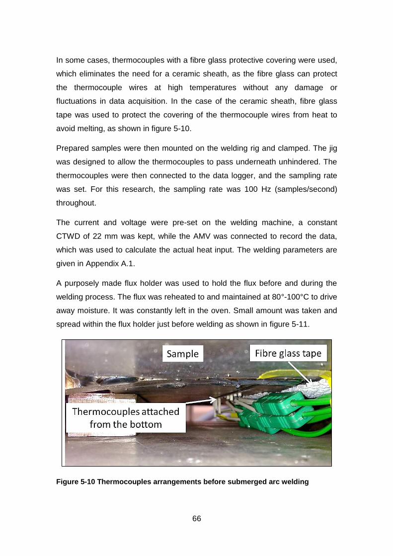
66

In some cases, thermocouples with a fibre glass protective covering were used,

which eliminates the need for a ceramic sheath, as the fibre glass can protect

the thermocouple wires at high temperatures without any damage or

fluctuations in data acquisition. In the case of the ceramic sheath, fibre glass

tape was used to protect the covering of the thermocouple wires from heat to

avoid melting, as shown in figure 5-10.

Prepared samples were then mounted on the welding rig and clamped. The jig

was designed to allow the thermocouples to pass underneath unhindered. The

thermocouples were then connected to the data logger, and the sampling rate

was set. For this research, the sampling rate was 100 Hz (samples/second)

throughout.

The current and voltage were pre-set on the welding machine, a constant

CTWD of 22 mm was kept, while the AMV was connected to record the data,

which was used to calculate the actual heat input. The welding parameters are

given in Appendix A.1.

A purposely made flux holder was used to hold the flux before and during the

welding process. The flux was reheated to and maintained at 80°-100°C to drive

away moisture. It was constantly left in the oven. Small amount was taken and

spread within the flux holder just before welding as shown in figure 5-11.

Figure 5-10 Thermocouples arrangements before submerged arc welding

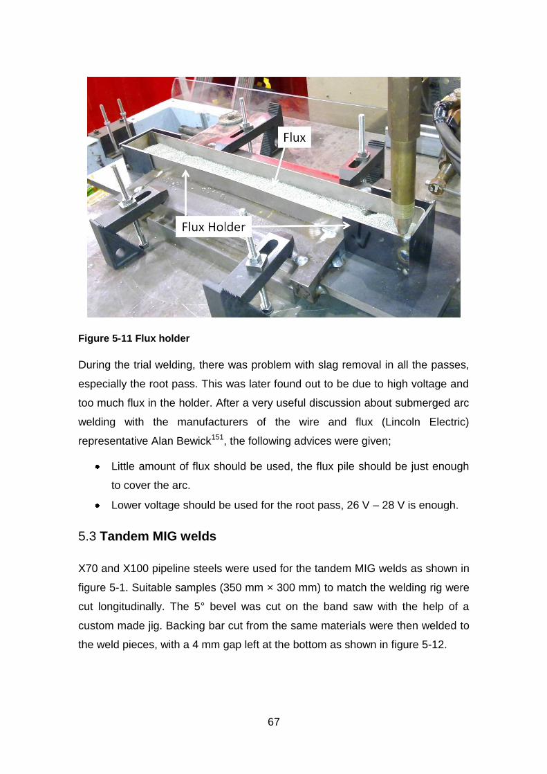
67

Figure 5-11 Flux holder

During the trial welding, there was problem with slag removal in all the passes,

especially the root pass. This was later found out to be due to high voltage and

too much flux in the holder. After a very useful discussion about submerged arc

welding with the manufacturers of the wire and flux (Lincoln Electric)

representative Alan Bewick151, the following advices were given;

Little amount of flux should be used, the flux pile should be just enough

to cover the arc.

Lower voltage should be used for the root pass, 26 V – 28 V is enough.

Tandem MIG welds 5.3

X70 and X100 pipeline steels were used for the tandem MIG welds as shown in

figure 5-1. Suitable samples (350 mm × 300 mm) to match the welding rig were

cut longitudinally. The 5° bevel was cut on the band saw with the help of a

custom made jig. Backing bar cut from the same materials were then welded to

the weld pieces, with a 4 mm gap left at the bottom as shown in figure 5-12.

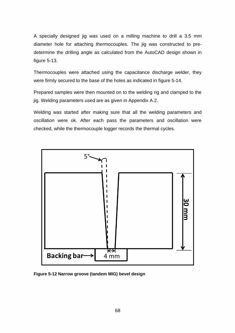
68

A specially designed jig was used on a milling machine to drill a 3.5 mm

diameter hole for attaching thermocouples. The jig was constructed to pre-

determine the drilling angle as calculated from the AutoCAD design shown in

figure 5-13.

Thermocouples were attached using the capacitance discharge welder, they

were firmly secured to the base of the holes as indicated in figure 5-14.

Prepared samples were then mounted on to the welding rig and clamped to the

jig. Welding parameters used are as given in Appendix A.2.

Welding was started after making sure that all the welding parameters and

oscillation were ok. After each pass the parameters and oscillation were

checked, while the thermocouple logger records the thermal cycles.

Figure 5-12 Narrow groove (tandem MIG) bevel design

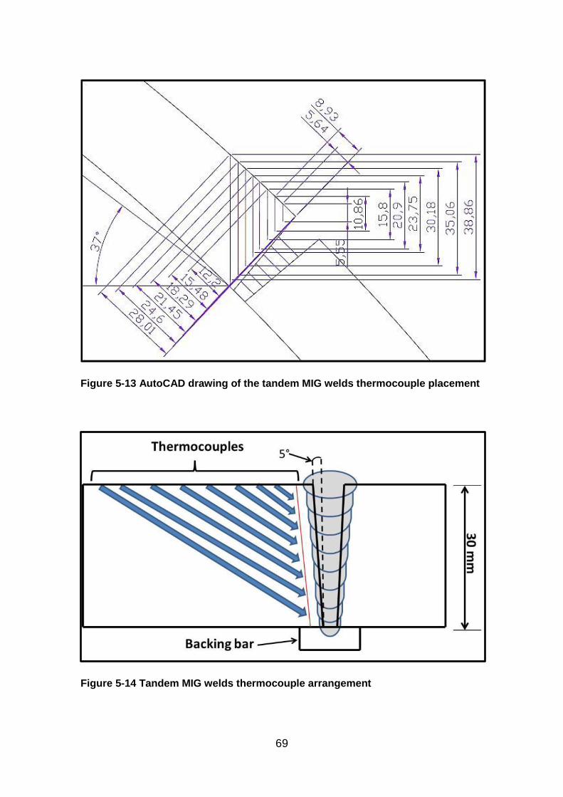
69

Figure 5-13 AutoCAD drawing of the tandem MIG welds thermocouple placement

Figure 5-14 Tandem MIG welds thermocouple arrangement

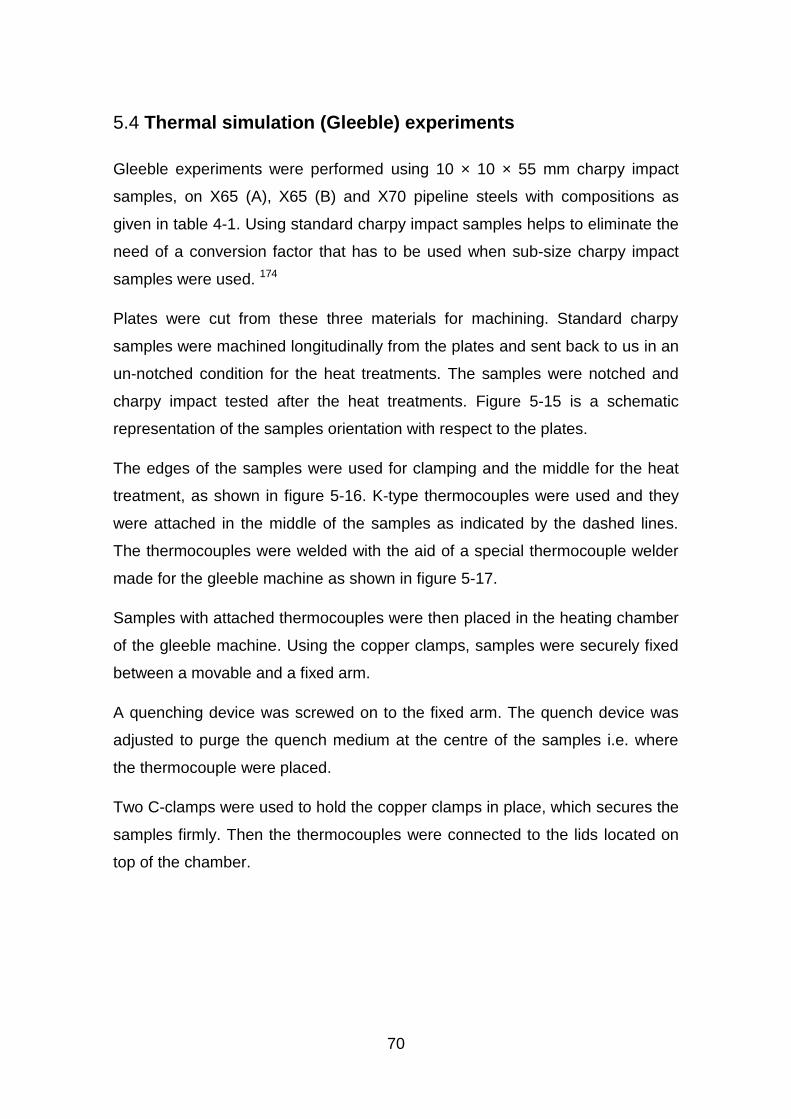
70

Thermal simulation (Gleeble) experiments 5.4

Gleeble experiments were performed using 10 × 10 × 55 mm charpy impact

samples, on X65 (A), X65 (B) and X70 pipeline steels with compositions as

given in table 4-1. Using standard charpy impact samples helps to eliminate the

need of a conversion factor that has to be used when sub-size charpy impact

samples were used. 174

Plates were cut from these three materials for machining. Standard charpy

samples were machined longitudinally from the plates and sent back to us in an

un-notched condition for the heat treatments. The samples were notched and

charpy impact tested after the heat treatments. Figure 5-15 is a schematic

representation of the samples orientation with respect to the plates.

The edges of the samples were used for clamping and the middle for the heat

treatment, as shown in figure 5-16. K-type thermocouples were used and they

were attached in the middle of the samples as indicated by the dashed lines.

The thermocouples were welded with the aid of a special thermocouple welder

made for the gleeble machine as shown in figure 5-17.

Samples with attached thermocouples were then placed in the heating chamber

of the gleeble machine. Using the copper clamps, samples were securely fixed

between a movable and a fixed arm.

A quenching device was screwed on to the fixed arm. The quench device was

adjusted to purge the quench medium at the centre of the samples i.e. where

the thermocouple were placed.

Two C-clamps were used to hold the copper clamps in place, which secures the

samples firmly. Then the thermocouples were connected to the lids located on

top of the chamber.

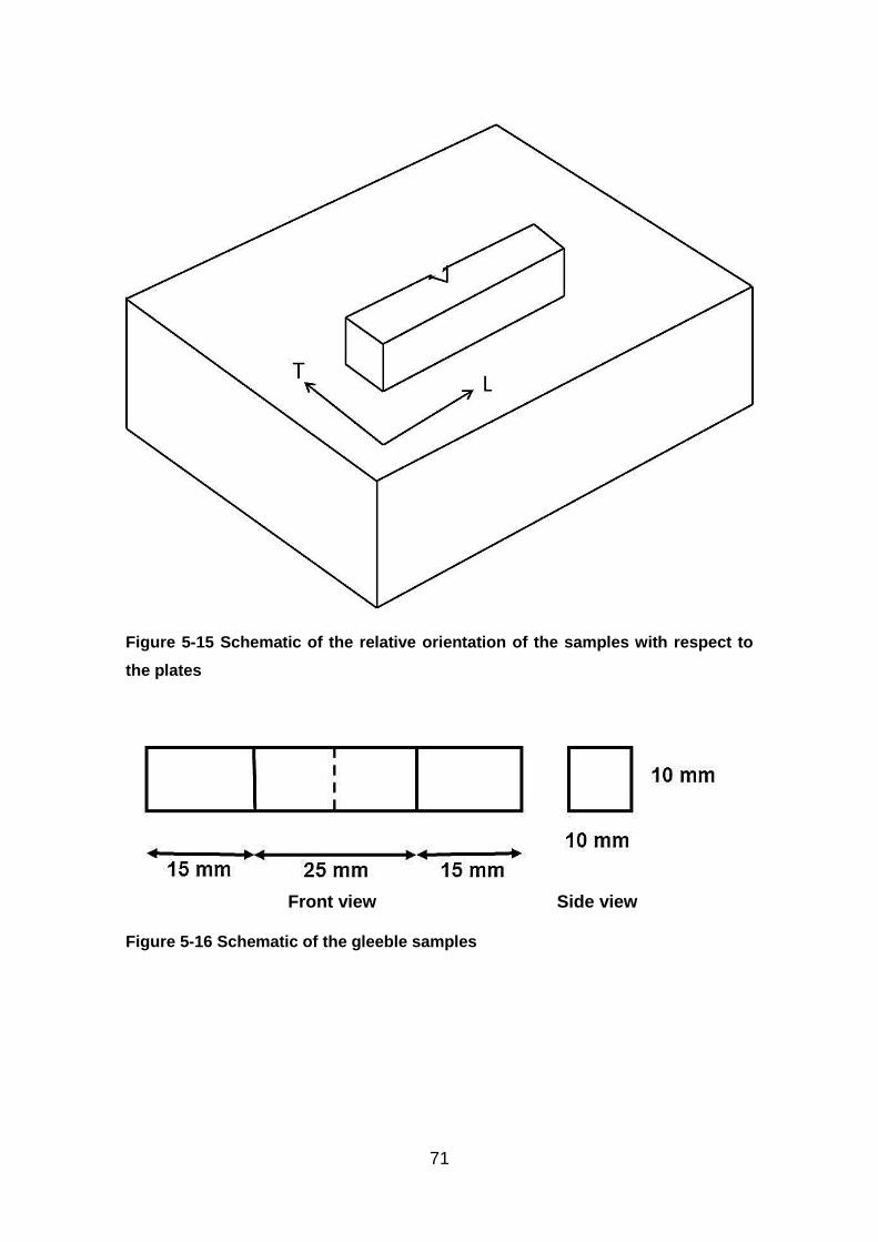
71

Figure 5-15 Schematic of the relative orientation of the samples with respect to

the plates

Figure 5-16 Schematic of the gleeble samples

Front view Side view

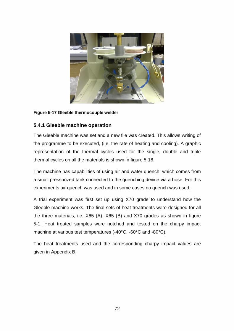
72

Figure 5-17 Gleeble thermocouple welder

5.4.1 Gleeble machine operation

The Gleeble machine was set and a new file was created. This allows writing of

the programme to be executed, (i.e. the rate of heating and cooling). A graphic

representation of the thermal cycles used for the single, double and triple

thermal cycles on all the materials is shown in figure 5-18.

The machine has capabilities of using air and water quench, which comes from

a small pressurized tank connected to the quenching device via a hose. For this

experiments air quench was used and in some cases no quench was used.

A trial experiment was first set up using X70 grade to understand how the

Gleeble machine works. The final sets of heat treatments were designed for all

the three materials, i.e. X65 (A), X65 (B) and X70 grades as shown in figure

5-1. Heat treated samples were notched and tested on the charpy impact

machine at various test temperatures (-40°C, -60°C and -80°C).

The heat treatments used and the corresponding charpy impact values are

given in Appendix B.

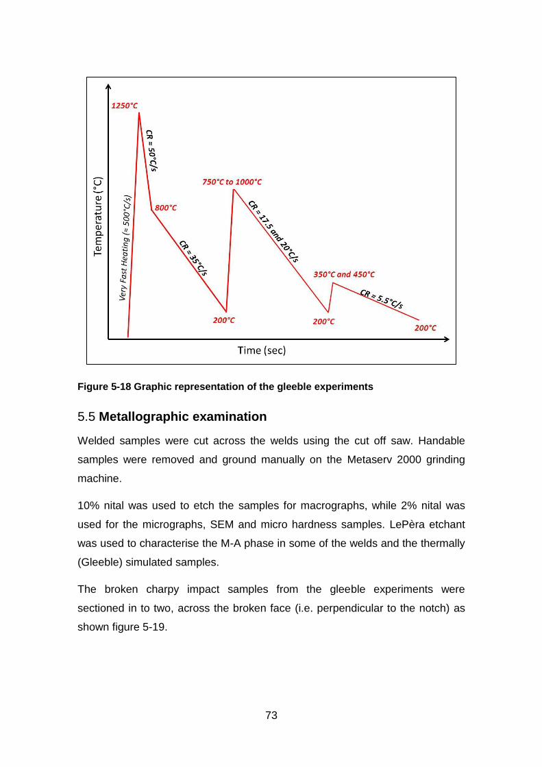
73

Figure 5-18 Graphic representation of the gleeble experiments

Metallographic examination 5.5

Welded samples were cut across the welds using the cut off saw. Handable

samples were removed and ground manually on the Metaserv 2000 grinding

machine.

10% nital was used to etch the samples for macrographs, while 2% nital was

used for the micrographs, SEM and micro hardness samples. LePèra etchant

was used to characterise the M-A phase in some of the welds and the thermally

(Gleeble) simulated samples.

The broken charpy impact samples from the gleeble experiments were

sectioned in to two, across the broken face (i.e. perpendicular to the notch) as

shown figure 5-19.

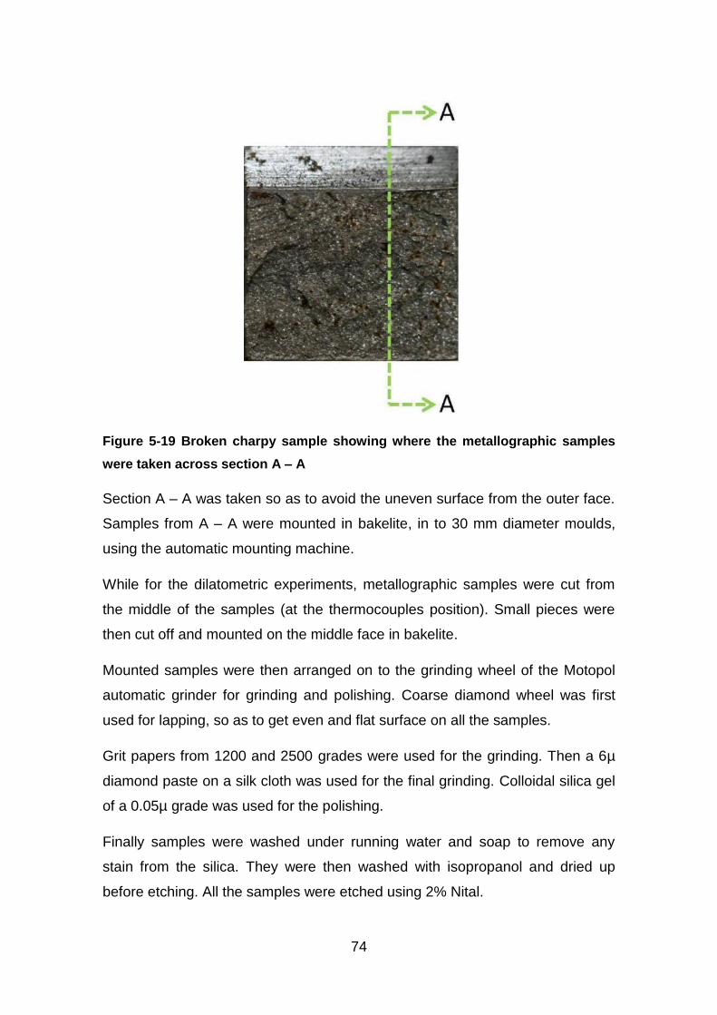
74

Figure 5-19 Broken charpy sample showing where the metallographic samples

were taken across section A – A

Section A – A was taken so as to avoid the uneven surface from the outer face.

Samples from A – A were mounted in bakelite, in to 30 mm diameter moulds,

using the automatic mounting machine.

While for the dilatometric experiments, metallographic samples were cut from

the middle of the samples (at the thermocouples position). Small pieces were

then cut off and mounted on the middle face in bakelite.

Mounted samples were then arranged on to the grinding wheel of the Motopol

automatic grinder for grinding and polishing. Coarse diamond wheel was first

used for lapping, so as to get even and flat surface on all the samples.

Grit papers from 1200 and 2500 grades were used for the grinding. Then a 6µ

diamond paste on a silk cloth was used for the final grinding. Colloidal silica gel

of a 0.05µ grade was used for the polishing.

Finally samples were washed under running water and soap to remove any

stain from the silica. They were then washed with isopropanol and dried up

before etching. All the samples were etched using 2% Nital.

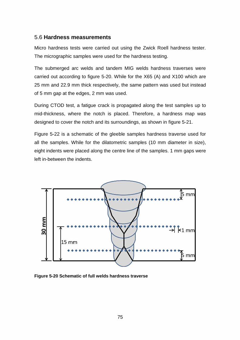
75

Hardness measurements 5.6

Micro hardness tests were carried out using the Zwick Roell hardness tester.

The micrographic samples were used for the hardness testing.

The submerged arc welds and tandem MIG welds hardness traverses were

carried out according to figure 5-20. While for the X65 (A) and X100 which are

25 mm and 22.9 mm thick respectively, the same pattern was used but instead

of 5 mm gap at the edges, 2 mm was used.

During CTOD test, a fatigue crack is propagated along the test samples up to

mid-thickness, where the notch is placed. Therefore, a hardness map was

designed to cover the notch and its surroundings, as shown in figure 5-21.

Figure 5-22 is a schematic of the gleeble samples hardness traverse used for

all the samples. While for the dilatometric samples (10 mm diameter in size),

eight indents were placed along the centre line of the samples. 1 mm gaps were

left in-between the indents.

Figure 5-20 Schematic of full welds hardness traverse

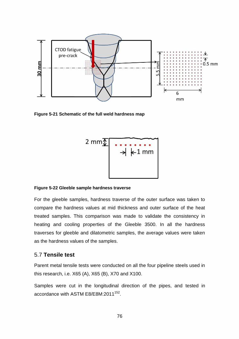
76

Figure 5-21 Schematic of the full weld hardness map

Figure 5-22 Gleeble sample hardness traverse

For the gleeble samples, hardness traverse of the outer surface was taken to

compare the hardness values at mid thickness and outer surface of the heat

treated samples. This comparison was made to validate the consistency in

heating and cooling properties of the Gleeble 3500. In all the hardness

traverses for gleeble and dilatometric samples, the average values were taken

as the hardness values of the samples.

Tensile test 5.7

Parent metal tensile tests were conducted on all the four pipeline steels used in

this research, i.e. X65 (A), X65 (B), X70 and X100.

Samples were cut in the longitudinal direction of the pipes, and tested in

accordance with ASTM E8/E8M:2011152.

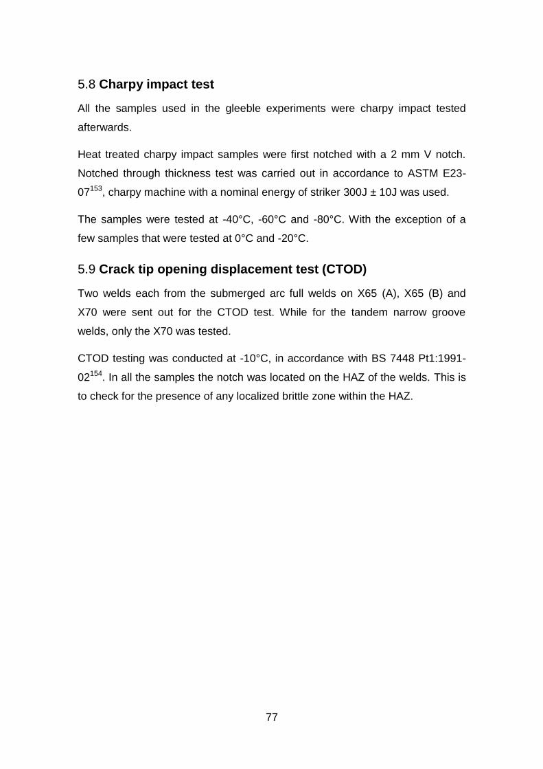
77

Charpy impact test 5.8

All the samples used in the gleeble experiments were charpy impact tested

afterwards.

Heat treated charpy impact samples were first notched with a 2 mm V notch.

Notched through thickness test was carried out in accordance to ASTM E23-

07153, charpy machine with a nominal energy of striker 300J ± 10J was used.

The samples were tested at -40°C, -60°C and -80°C. With the exception of a

few samples that were tested at 0°C and -20°C.

Crack tip opening displacement test (CTOD) 5.9

Two welds each from the submerged arc full welds on X65 (A), X65 (B) and

X70 were sent out for the CTOD test. While for the tandem narrow groove

welds, only the X70 was tested.

CTOD testing was conducted at -10°C, in accordance with BS 7448 Pt1:1991-

02154. In all the samples the notch was located on the HAZ of the welds. This is

to check for the presence of any localized brittle zone within the HAZ.

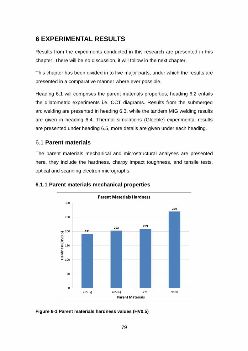
79

6 EXPERIMENTAL RESULTS

Results from the experiments conducted in this research are presented in this

chapter. There will be no discussion, it will follow in the next chapter.

This chapter has been divided in to five major parts, under which the results are

presented in a comparative manner where ever possible.

Heading 6.1 will comprises the parent materials properties, heading 6.2 entails

the dilatometric experiments i.e. CCT diagrams. Results from the submerged

arc welding are presented in heading 6.3, while the tandem MIG welding results

are given in heading 6.4. Thermal simulations (Gleeble) experimental results

are presented under heading 6.5, more details are given under each heading.

Parent materials 6.1

The parent materials mechanical and microstructural analyses are presented

here, they include the hardness, charpy impact toughness, and tensile tests,

optical and scanning electron micrographs.

6.1.1 Parent materials mechanical properties

Figure 6-1 Parent materials hardness values (HV0.5)

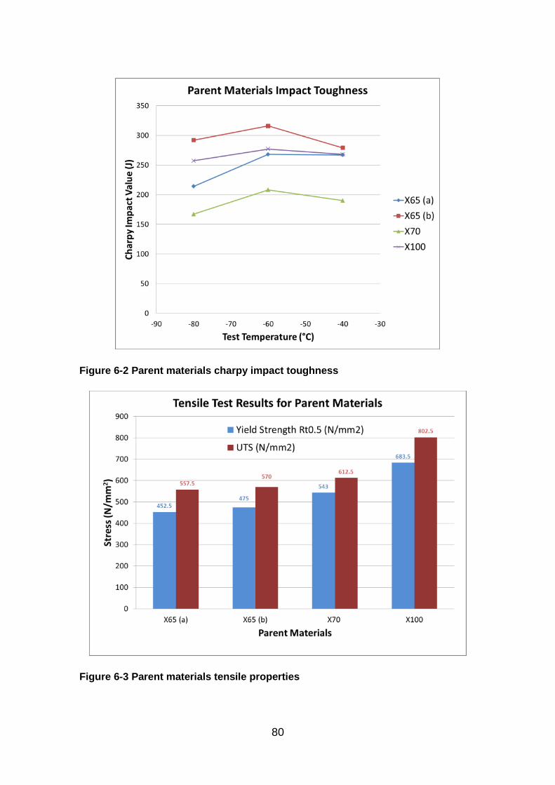
80

Figure 6-2 Parent materials charpy impact toughness

Figure 6-3 Parent materials tensile properties

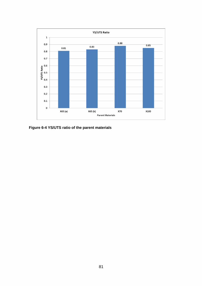
81

Figure 6-4 YS/UTS ratio of the parent materials

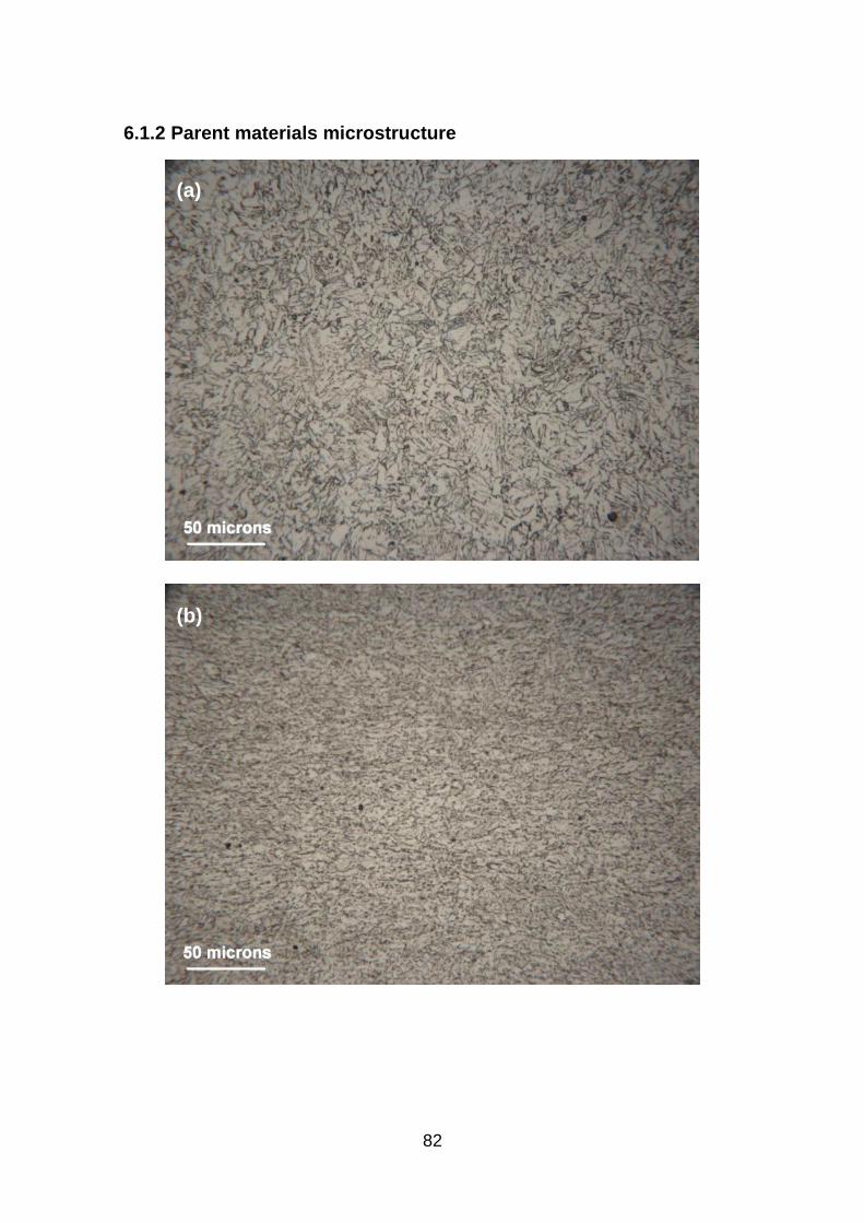
82

6.1.2 Parent materials microstructure

(a)

(b)

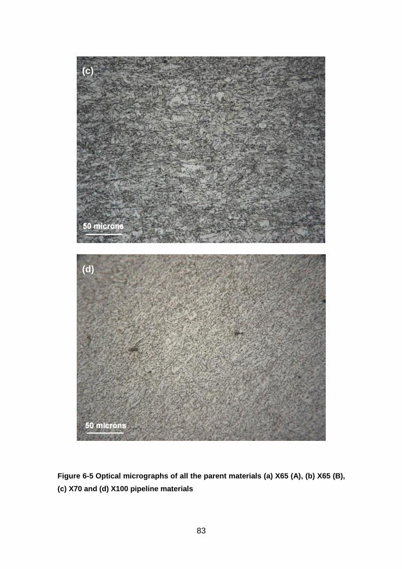
83

Figure 6-5 Optical micrographs of all the parent materials (a) X65 (A), (b) X65 (B),

(c) X70 and (d) X100 pipeline materials

(c)

(d)

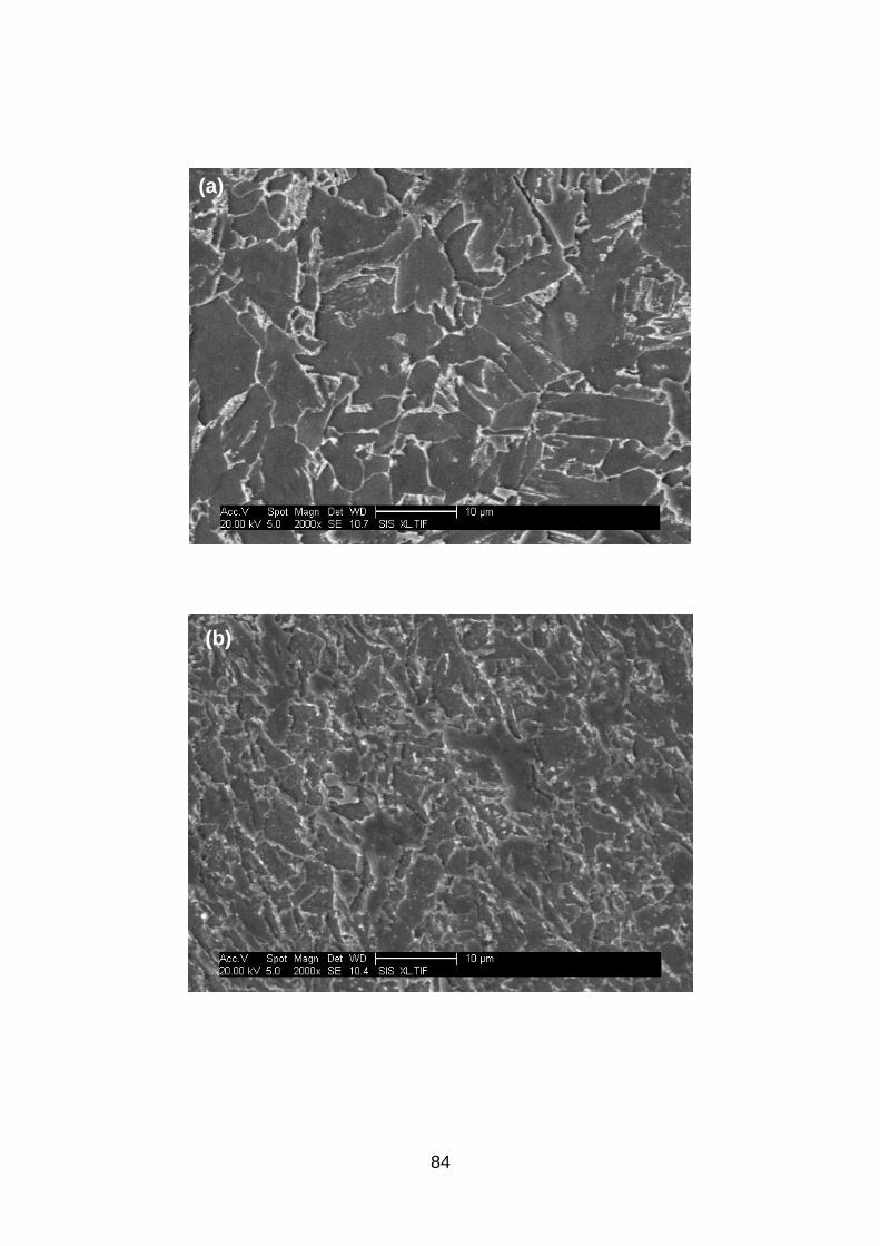
84

(a)

(b)

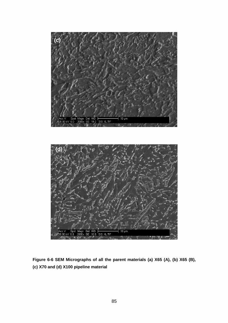
85

Figure 6-6 SEM Micrographs of all the parent materials (a) X65 (A), (b) X65 (B),

(c) X70 and (d) X100 pipeline material

(c)

(d)

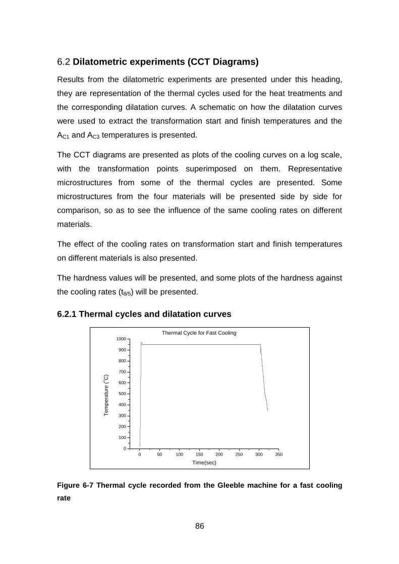
86

Dilatometric experiments (CCT Diagrams) 6.2

Results from the dilatometric experiments are presented under this heading,

they are representation of the thermal cycles used for the heat treatments and

the corresponding dilatation curves. A schematic on how the dilatation curves

were used to extract the transformation start and finish temperatures and the

AC1 and AC3 temperatures is presented.

The CCT diagrams are presented as plots of the cooling curves on a log scale,

with the transformation points superimposed on them. Representative

microstructures from some of the thermal cycles are presented. Some

microstructures from the four materials will be presented side by side for

comparison, so as to see the influence of the same cooling rates on different

materials.

The effect of the cooling rates on transformation start and finish temperatures

on different materials is also presented.

The hardness values will be presented, and some plots of the hardness against

the cooling rates (t8/5) will be presented.

6.2.1 Thermal cycles and dilatation curves

Figure 6-7 Thermal cycle recorded from the Gleeble machine for a fast cooling

rate

0 50 100 150 200 250 300 350

0

100

200

300

400

500

600

700

800

900

1000

Te

mp

era

ture

(oC

)

Time(sec)

Thermal Cycle for Fast Cooling

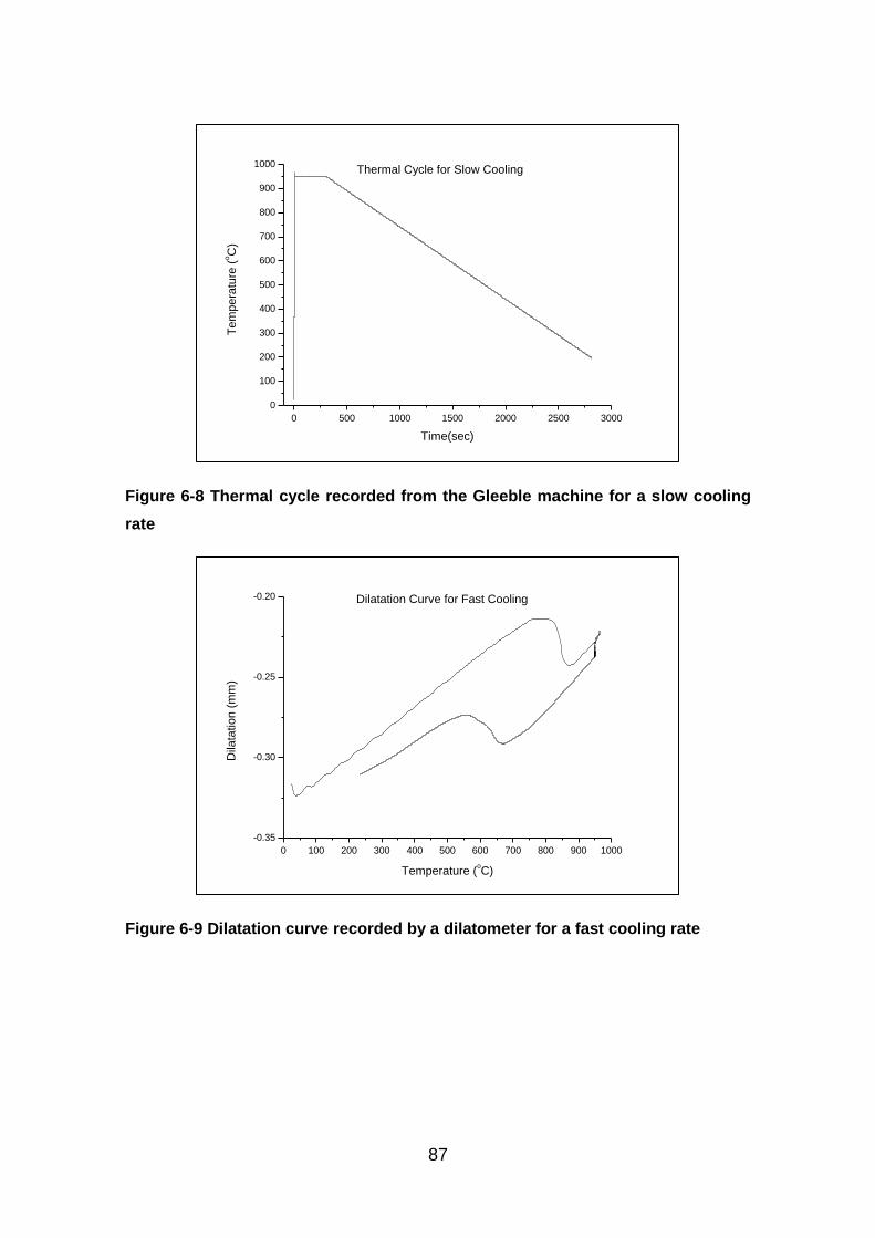
87

Figure 6-8 Thermal cycle recorded from the Gleeble machine for a slow cooling

rate

Figure 6-9 Dilatation curve recorded by a dilatometer for a fast cooling rate

0 500 1000 1500 2000 2500 3000

0

100

200

300

400

500

600

700

800

900

1000

Te

mp

era

ture

(oC

)

Time(sec)

Thermal Cycle for Slow Cooling

0 100 200 300 400 500 600 700 800 900 1000

-0.35

-0.30

-0.25

-0.20

Dila

tatio

n (

mm

)

Temperature (oC)

Dilatation Curve for Fast Cooling

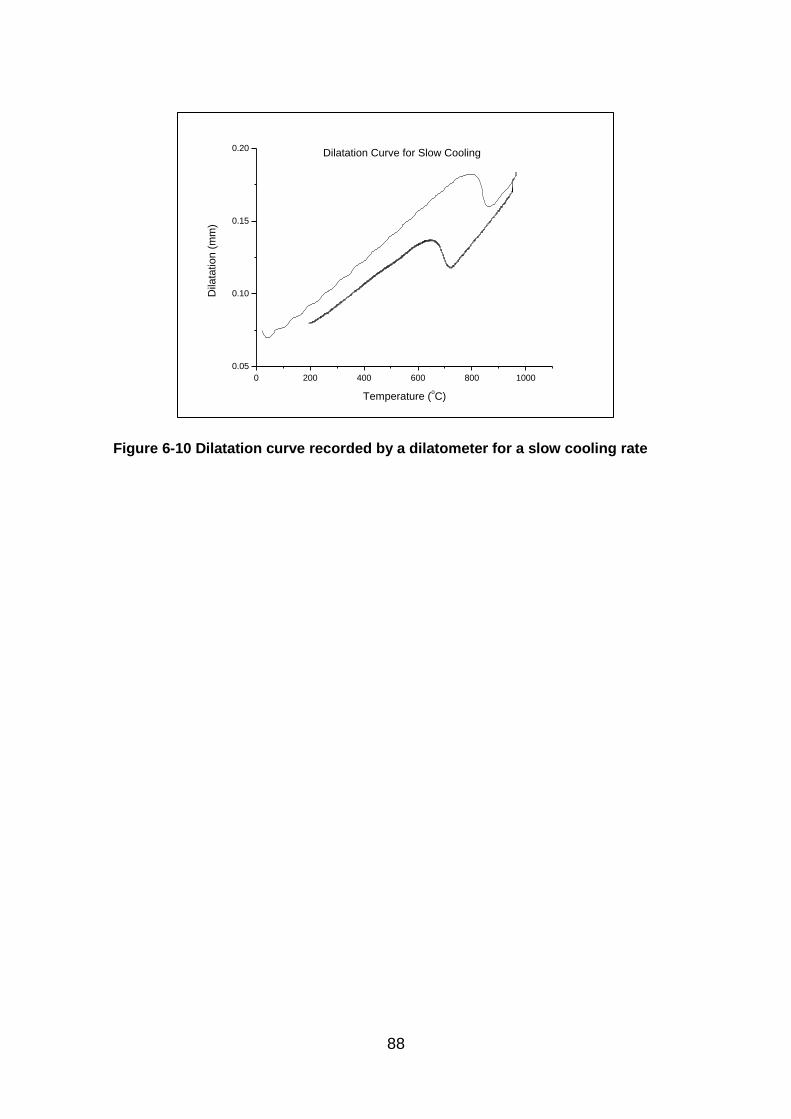
88

Figure 6-10 Dilatation curve recorded by a dilatometer for a slow cooling rate

0 200 400 600 800 1000

0.05

0.10

0.15

0.20

Dila

tatio

n (

mm

)

Temperature (oC)

Dilatation Curve for Slow Cooling

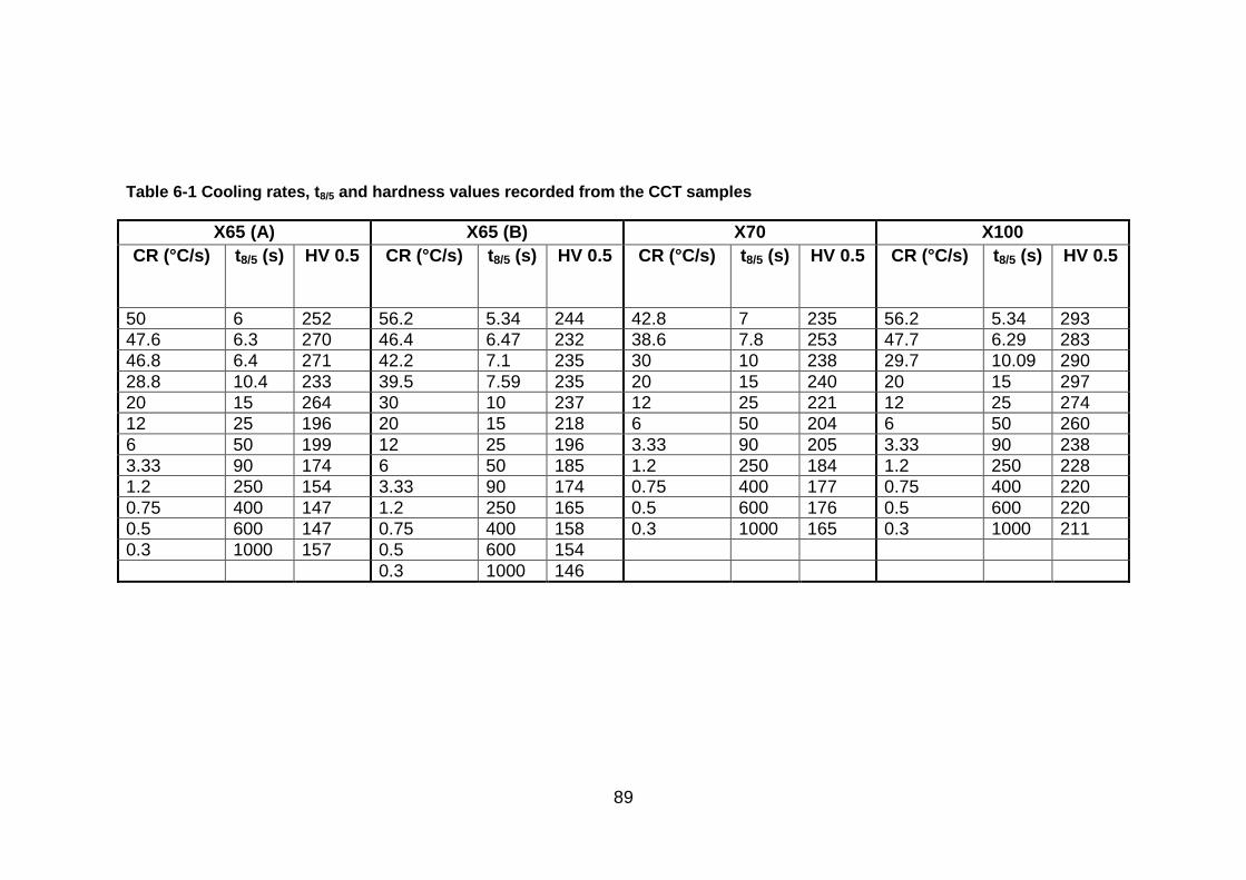
89

Table 6-1 Cooling rates, t8/5 and hardness values recorded from the CCT samples

X65 (A) X65 (B) X70 X100

CR (°C/s) t8/5 (s) HV 0.5 CR (°C/s) t8/5 (s) HV 0.5 CR (°C/s) t8/5 (s) HV 0.5 CR (°C/s) t8/5 (s) HV 0.5

50 6 252 56.2 5.34 244 42.8 7 235 56.2 5.34 293

47.6 6.3 270 46.4 6.47 232 38.6 7.8 253 47.7 6.29 283

46.8 6.4 271 42.2 7.1 235 30 10 238 29.7 10.09 290

28.8 10.4 233 39.5 7.59 235 20 15 240 20 15 297

20 15 264 30 10 237 12 25 221 12 25 274

12 25 196 20 15 218 6 50 204 6 50 260

6 50 199 12 25 196 3.33 90 205 3.33 90 238

3.33 90 174 6 50 185 1.2 250 184 1.2 250 228

1.2 250 154 3.33 90 174 0.75 400 177 0.75 400 220

0.75 400 147 1.2 250 165 0.5 600 176 0.5 600 220

0.5 600 147 0.75 400 158 0.3 1000 165 0.3 1000 211

0.3 1000 157 0.5 600 154

0.3 1000 146

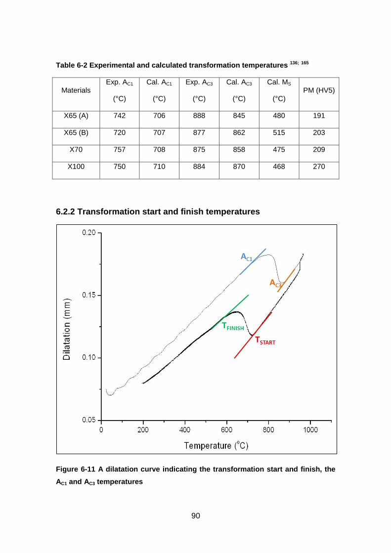
90

Table 6-2 Experimental and calculated transformation temperatures 136; 165

Materials Exp. AC1

(°C)

Cal. AC1

(°C)

Exp. AC3

(°C)

Cal. AC3

(°C)

Cal. MS

(°C) PM (HV5)

X65 (A) 742 706 888 845 480 191

X65 (B) 720 707 877 862 515 203

X70 757 708 875 858 475 209

X100 750 710 884 870 468 270

6.2.2 Transformation start and finish temperatures

Figure 6-11 A dilatation curve indicating the transformation start and finish, the

AC1 and AC3 temperatures

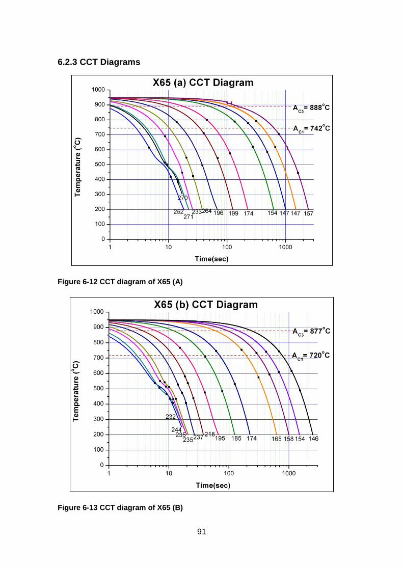
91

6.2.3 CCT Diagrams

Figure 6-12 CCT diagram of X65 (A)

Figure 6-13 CCT diagram of X65 (B)

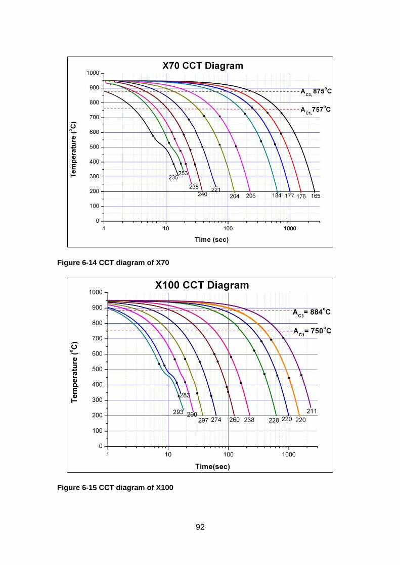
92

Figure 6-14 CCT diagram of X70

Figure 6-15 CCT diagram of X100

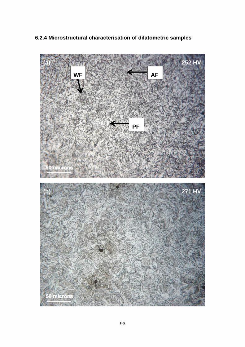
93

6.2.4 Microstructural characterisation of dilatometric samples

(a)

(b)

252 HV

271 HV

WF AF

PF

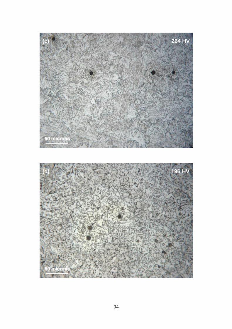
94

(d)

(c)

196 HV

264 HV

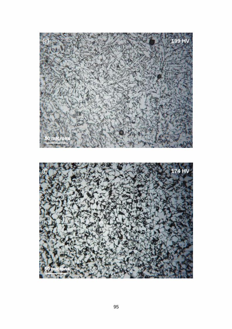
95

(e)

(f)

199 HV

174 HV

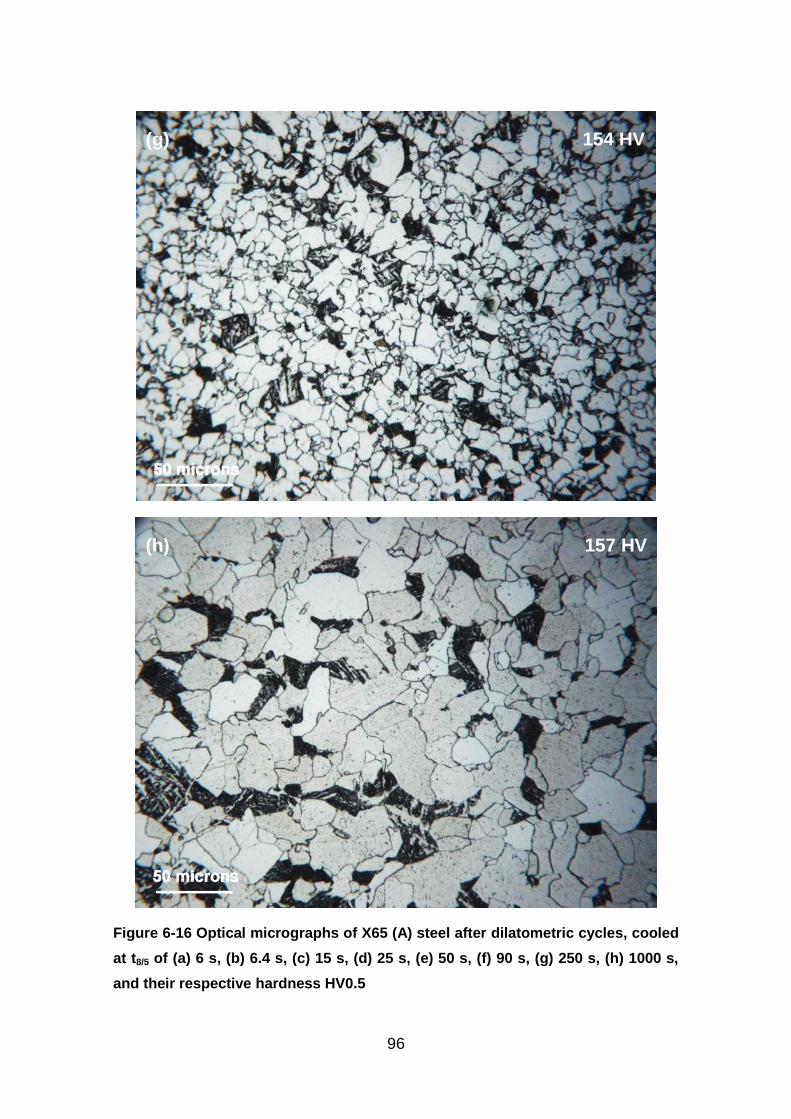
96

Figure 6-16 Optical micrographs of X65 (A) steel after dilatometric cycles, cooled

at t8/5 of (a) 6 s, (b) 6.4 s, (c) 15 s, (d) 25 s, (e) 50 s, (f) 90 s, (g) 250 s, (h) 1000 s,

and their respective hardness HV0.5

(h)

(g)

157 HV

154 HV

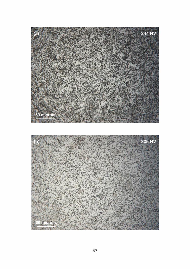
97

(b)

(a)

235 HV

244 HV

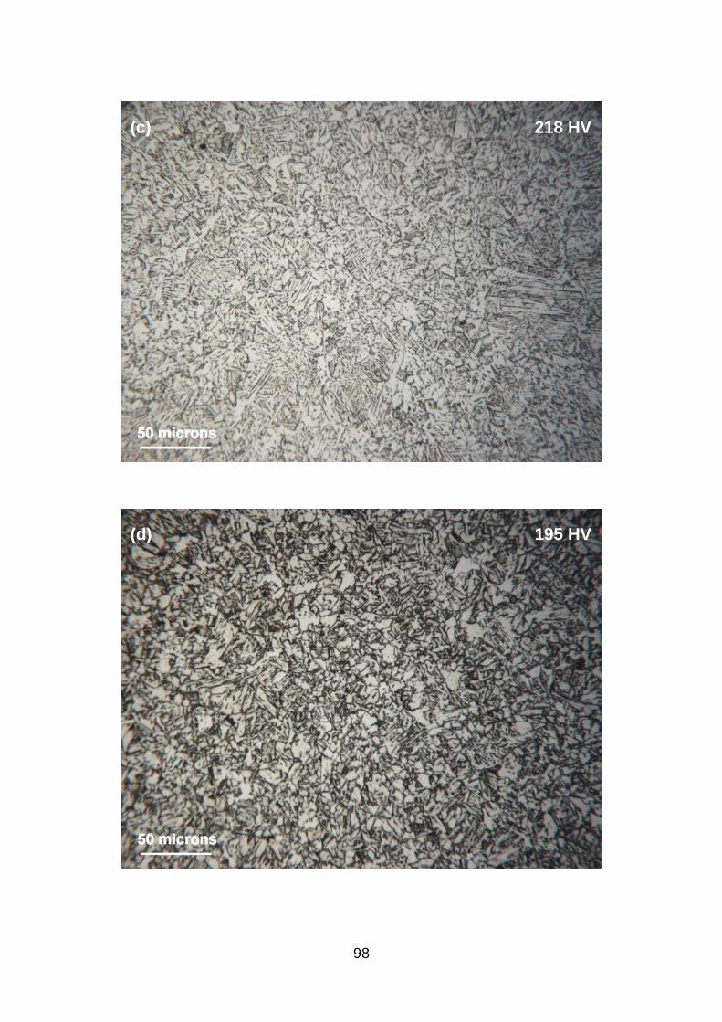
98

(d)

(c)

195 HV

218 HV

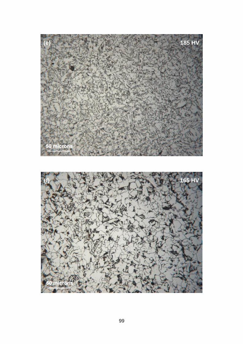
99

(f)

(e)

165 HV

185 HV

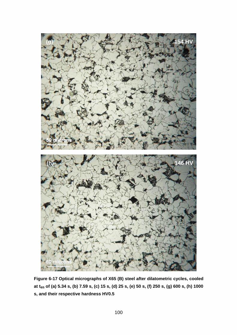
100

Figure 6-17 Optical micrographs of X65 (B) steel after dilatometric cycles, cooled

at t8/5 of (a) 5.34 s, (b) 7.59 s, (c) 15 s, (d) 25 s, (e) 50 s, (f) 250 s, (g) 600 s, (h) 1000

s, and their respective hardness HV0.5

(h)

(g)

146 HV

154 HV

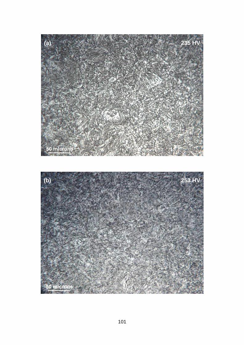
101

253 HV

235 HV

(b)

(a)

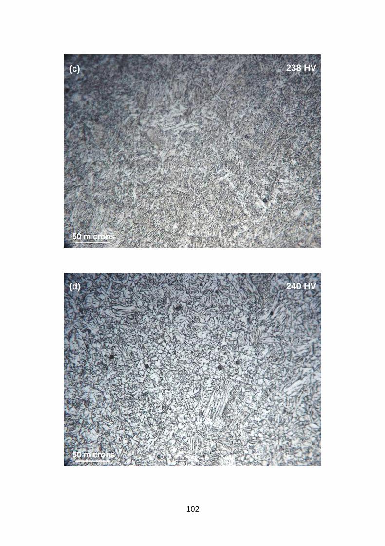
102

240 HV

238 HV

(d)

(c)

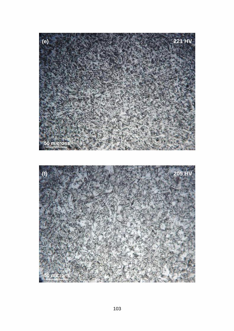
103

205 HV

221 HV

(f)

(e)

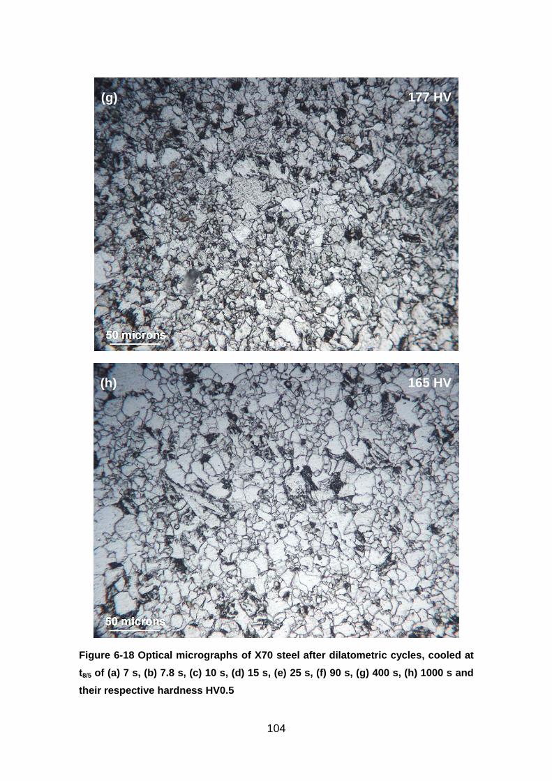
104

Figure 6-18 Optical micrographs of X70 steel after dilatometric cycles, cooled at

t8/5 of (a) 7 s, (b) 7.8 s, (c) 10 s, (d) 15 s, (e) 25 s, (f) 90 s, (g) 400 s, (h) 1000 s and

their respective hardness HV0.5

165 HV

177 HV

(h)

(g)

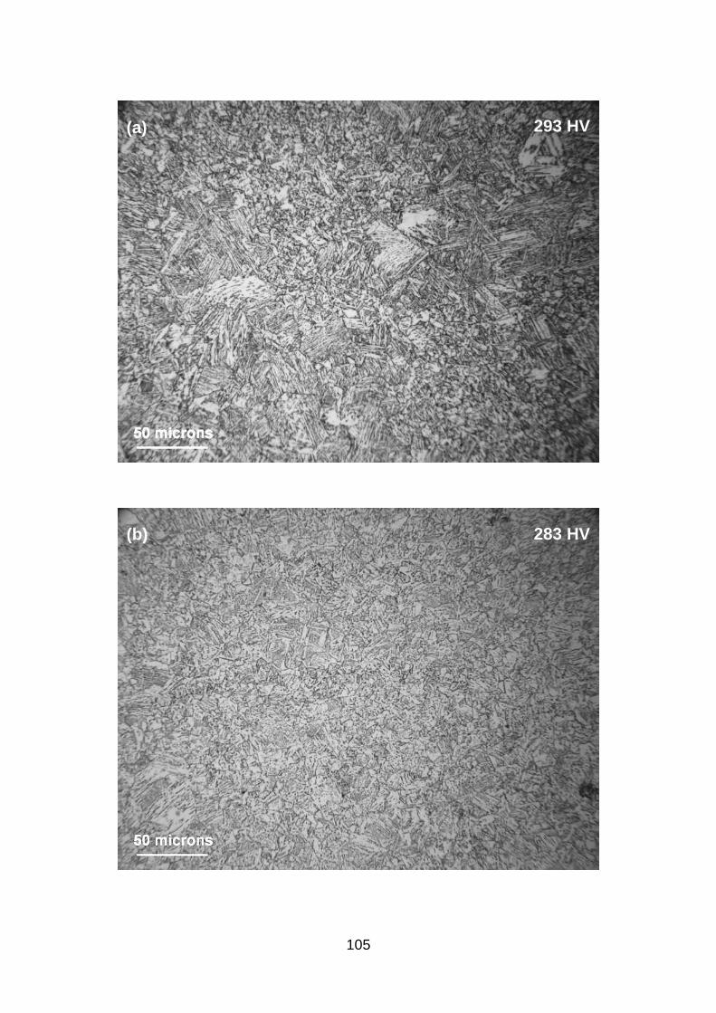
105

(b)

(a)

283 HV

293 HV

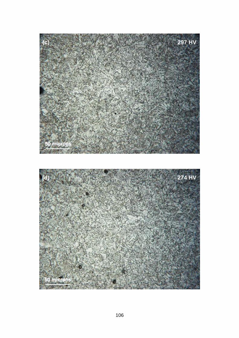
106

(d)

(c)

274 HV

297 HV

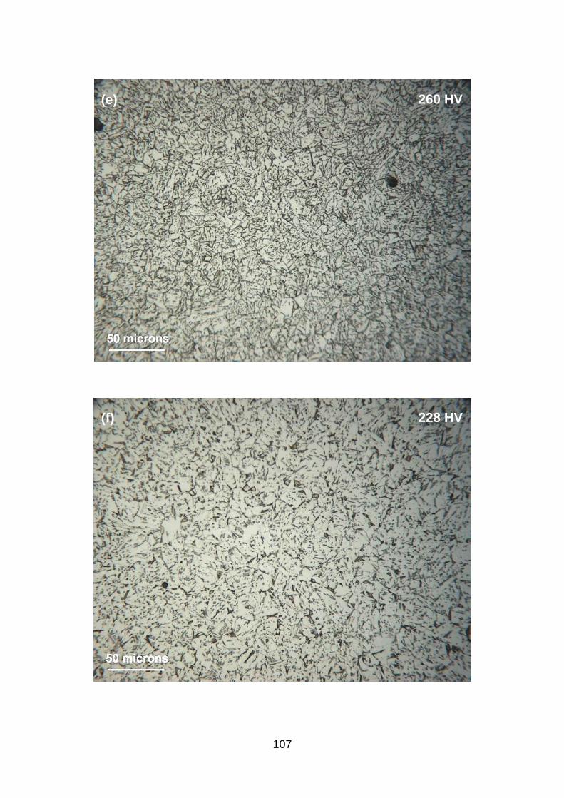
107

(f)

(e)

228 HV

260 HV

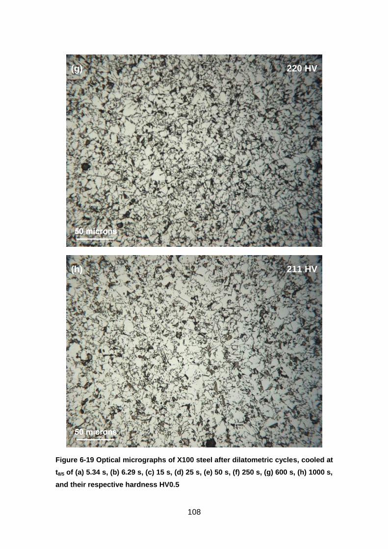
108

Figure 6-19 Optical micrographs of X100 steel after dilatometric cycles, cooled at

t8/5 of (a) 5.34 s, (b) 6.29 s, (c) 15 s, (d) 25 s, (e) 50 s, (f) 250 s, (g) 600 s, (h) 1000 s,

and their respective hardness HV0.5

(h)

(g)

211 HV

220 HV

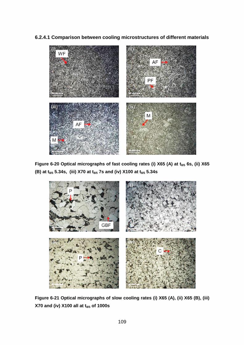
109

6.2.4.1 Comparison between cooling microstructures of different materials

Figure 6-20 Optical micrographs of fast cooling rates (i) X65 (A) at t8/5 6s, (ii) X65

(B) at t8/5 5.34s, (iii) X70 at t8/5 7s and (iv) X100 at t8/5 5.34s

Figure 6-21 Optical micrographs of slow cooling rates (i) X65 (A), (ii) X65 (B), (iii)

X70 and (iv) X100 all at t8/5 of 1000s

110

6.2.4.2 Heat treated microstructures

Figure 6-22 Optical micrographs of air quenched samples (a) X65 (A), (b) X65 (B),

(c) X70 and (d) X100

Figure 6-23 Optical micrographs of oil quenched samples (a) X65 (A), (b) X65 (B),

(c) X70 and (d) X100

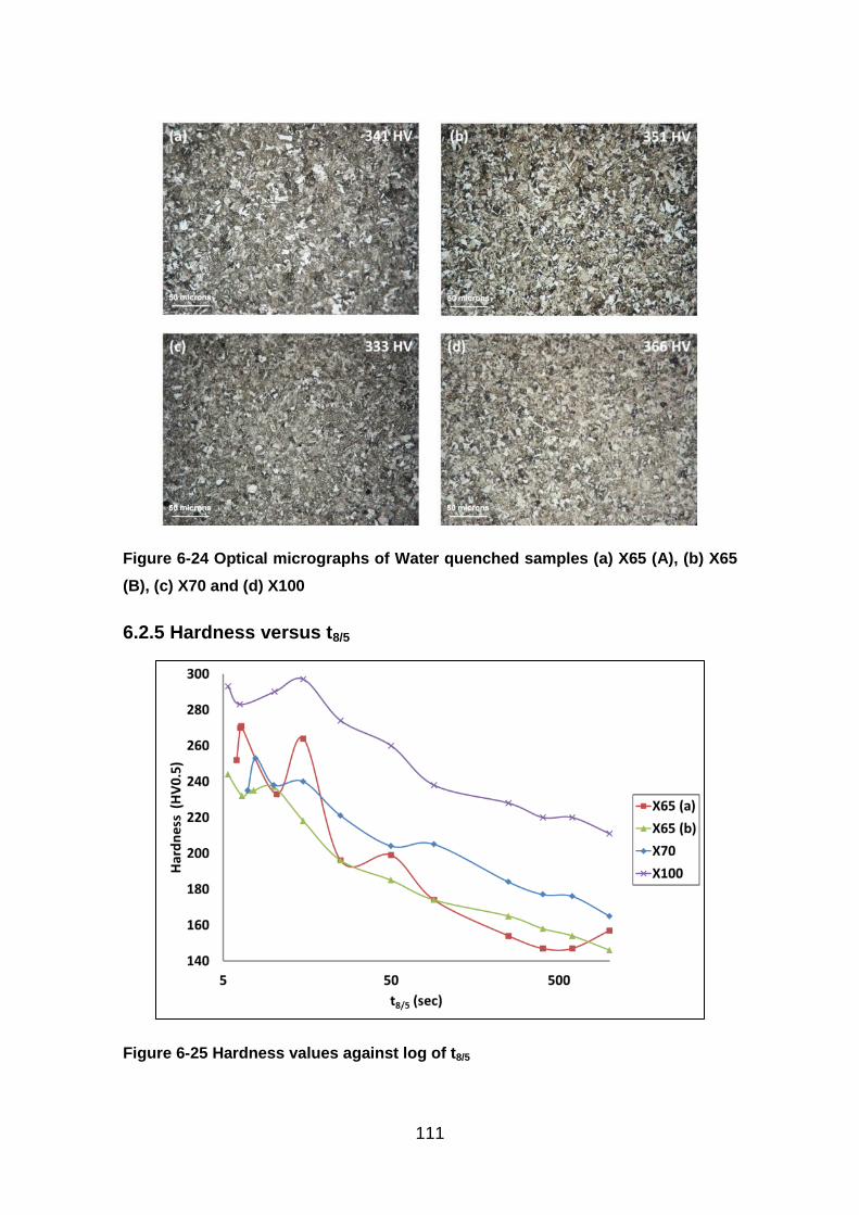
111

Figure 6-24 Optical micrographs of Water quenched samples (a) X65 (A), (b) X65

(B), (c) X70 and (d) X100

6.2.5 Hardness versus t8/5

Figure 6-25 Hardness values against log of t8/5

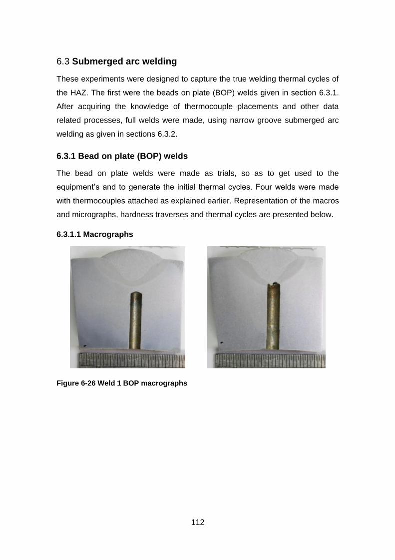
112

Submerged arc welding 6.3

These experiments were designed to capture the true welding thermal cycles of

the HAZ. The first were the beads on plate (BOP) welds given in section 6.3.1.

After acquiring the knowledge of thermocouple placements and other data

related processes, full welds were made, using narrow groove submerged arc

welding as given in sections 6.3.2.

6.3.1 Bead on plate (BOP) welds

The bead on plate welds were made as trials, so as to get used to the

equipment’s and to generate the initial thermal cycles. Four welds were made

with thermocouples attached as explained earlier. Representation of the macros

and micrographs, hardness traverses and thermal cycles are presented below.

6.3.1.1 Macrographs

Figure 6-26 Weld 1 BOP macrographs

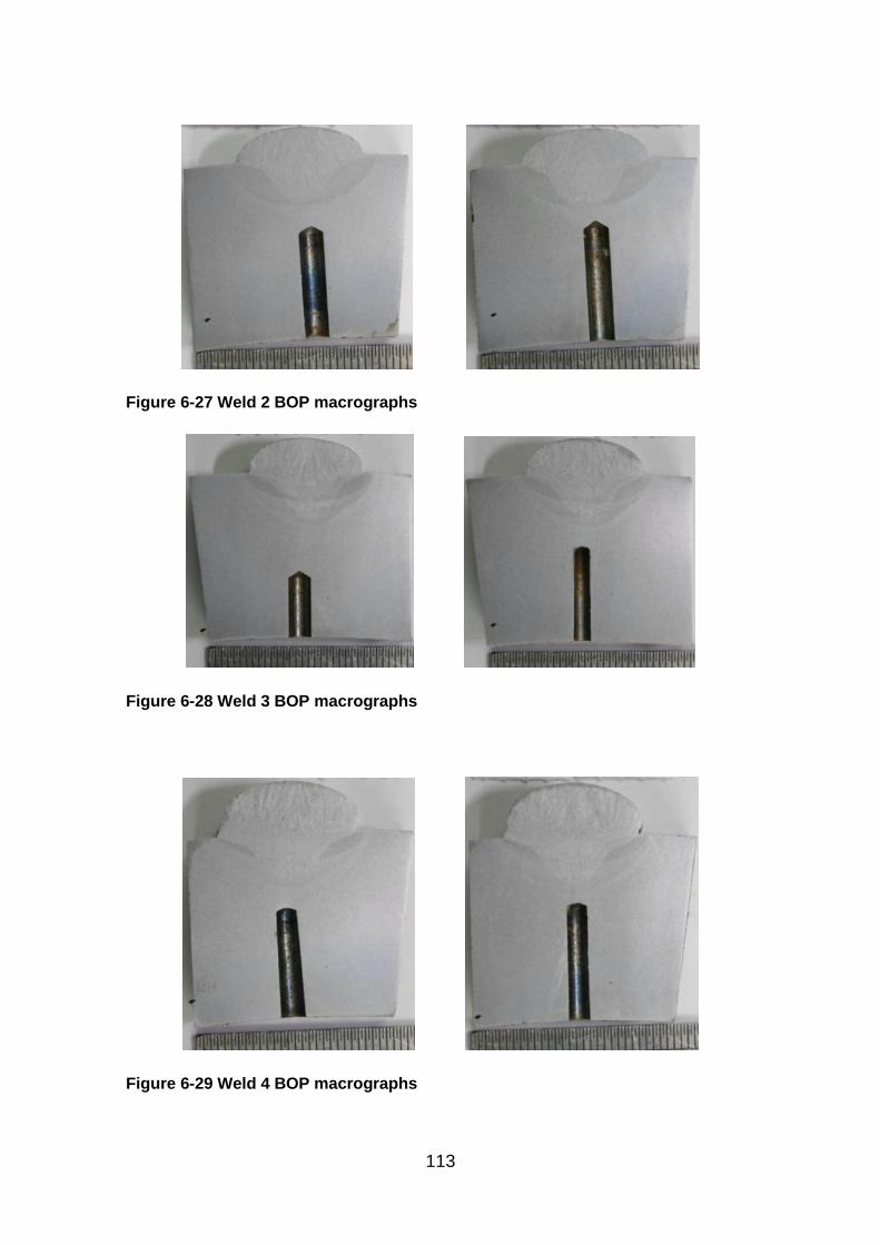
113

Figure 6-27 Weld 2 BOP macrographs

Figure 6-28 Weld 3 BOP macrographs

Figure 6-29 Weld 4 BOP macrographs

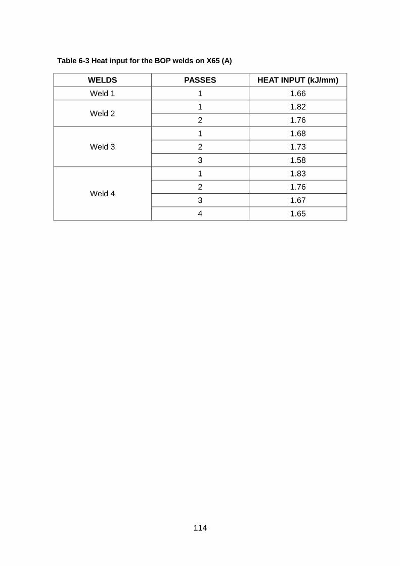
114

Table 6-3 Heat input for the BOP welds on X65 (A)

WELDS PASSES HEAT INPUT (kJ/mm)

Weld 1 1 1.66

Weld 2 1 1.82

2 1.76

Weld 3

1 1.68

2 1.73

3 1.58

Weld 4

1 1.83

2 1.76

3 1.67

4 1.65

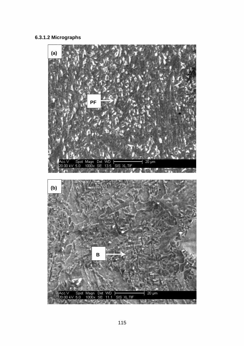
115

6.3.1.2 Micrographs

(a)

PF

B

(b)

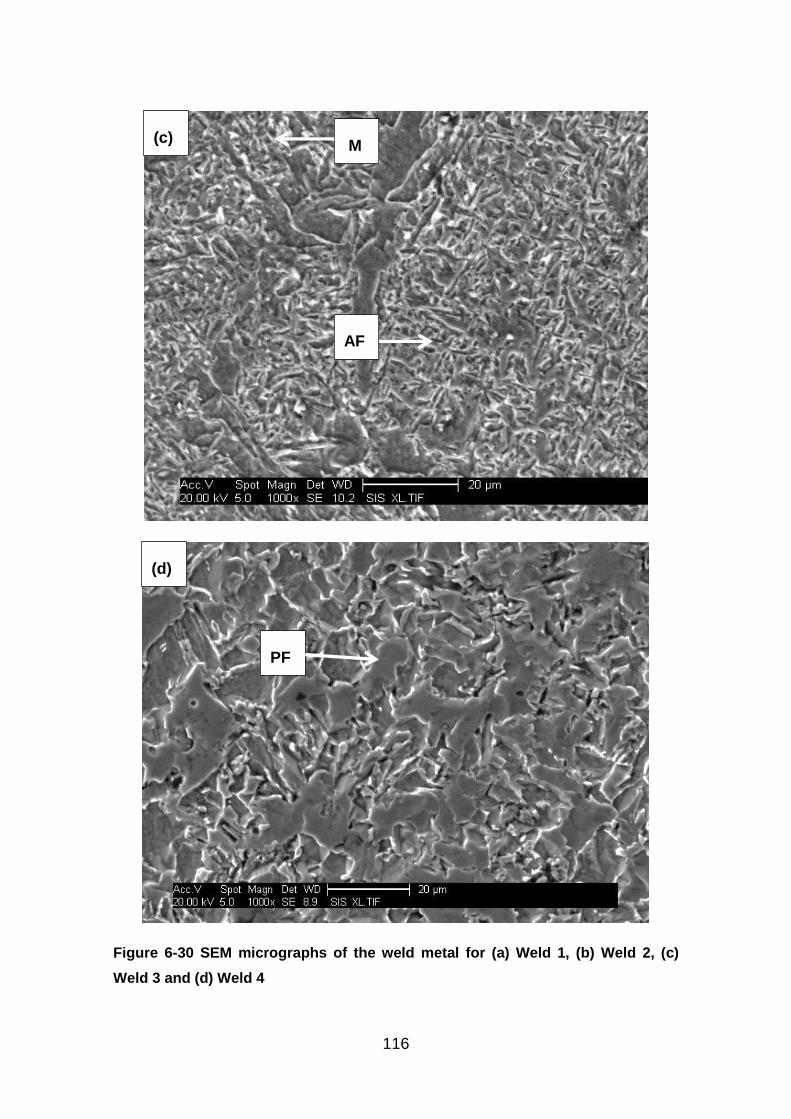
116

Figure 6-30 SEM micrographs of the weld metal for (a) Weld 1, (b) Weld 2, (c)

Weld 3 and (d) Weld 4

(c)

(d)

PF

AF

M

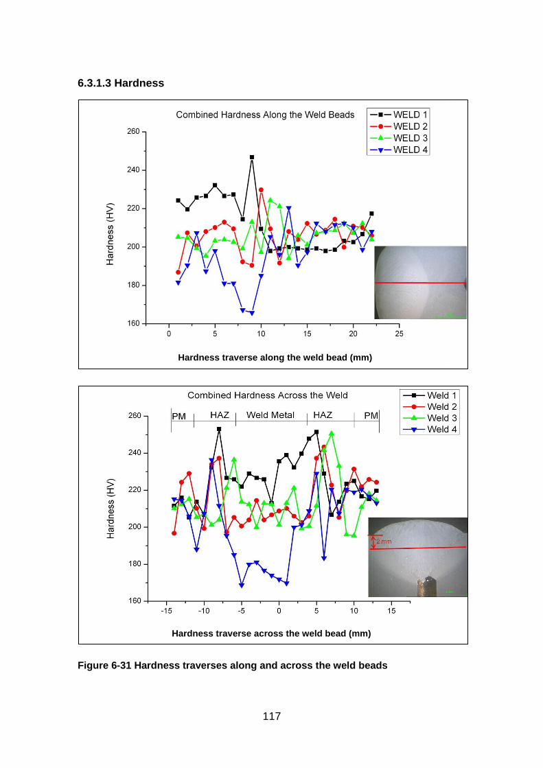
117

6.3.1.3 Hardness

Figure 6-31 Hardness traverses along and across the weld beads

Hardness traverse along the weld bead (mm)

Hardness traverse across the weld bead (mm)

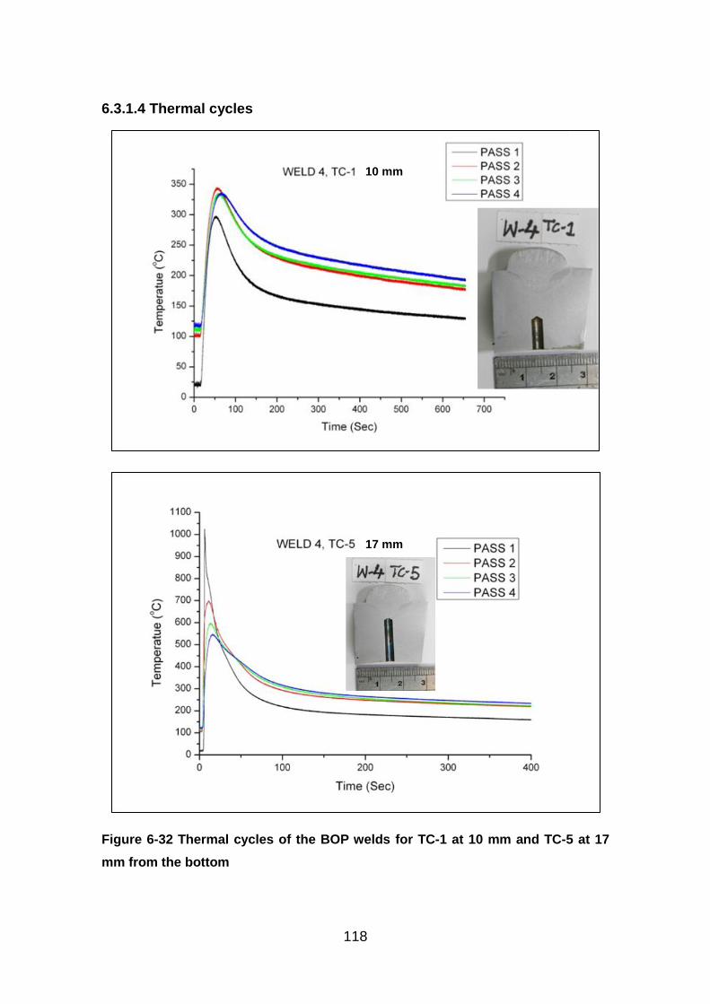
118

6.3.1.4 Thermal cycles

Figure 6-32 Thermal cycles of the BOP welds for TC-1 at 10 mm and TC-5 at 17

mm from the bottom

17 mm

10 mm

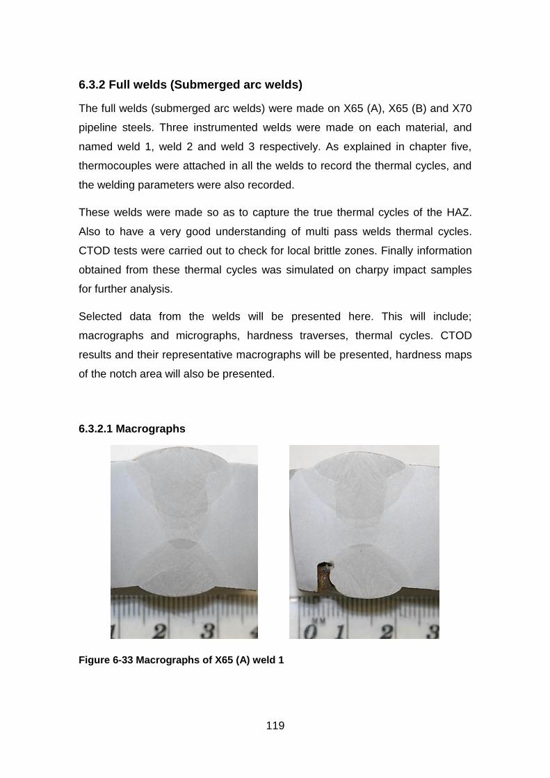
119

6.3.2 Full welds (Submerged arc welds)

The full welds (submerged arc welds) were made on X65 (A), X65 (B) and X70

pipeline steels. Three instrumented welds were made on each material, and

named weld 1, weld 2 and weld 3 respectively. As explained in chapter five,

thermocouples were attached in all the welds to record the thermal cycles, and

the welding parameters were also recorded.

These welds were made so as to capture the true thermal cycles of the HAZ.

Also to have a very good understanding of multi pass welds thermal cycles.

CTOD tests were carried out to check for local brittle zones. Finally information

obtained from these thermal cycles was simulated on charpy impact samples

for further analysis.

Selected data from the welds will be presented here. This will include;

macrographs and micrographs, hardness traverses, thermal cycles. CTOD

results and their representative macrographs will be presented, hardness maps

of the notch area will also be presented.

6.3.2.1 Macrographs

Figure 6-33 Macrographs of X65 (A) weld 1

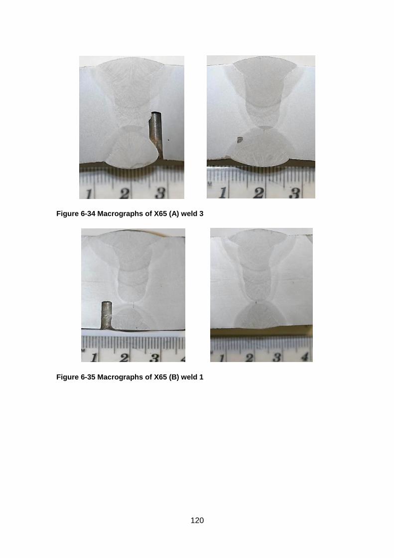
120

Figure 6-34 Macrographs of X65 (A) weld 3

Figure 6-35 Macrographs of X65 (B) weld 1

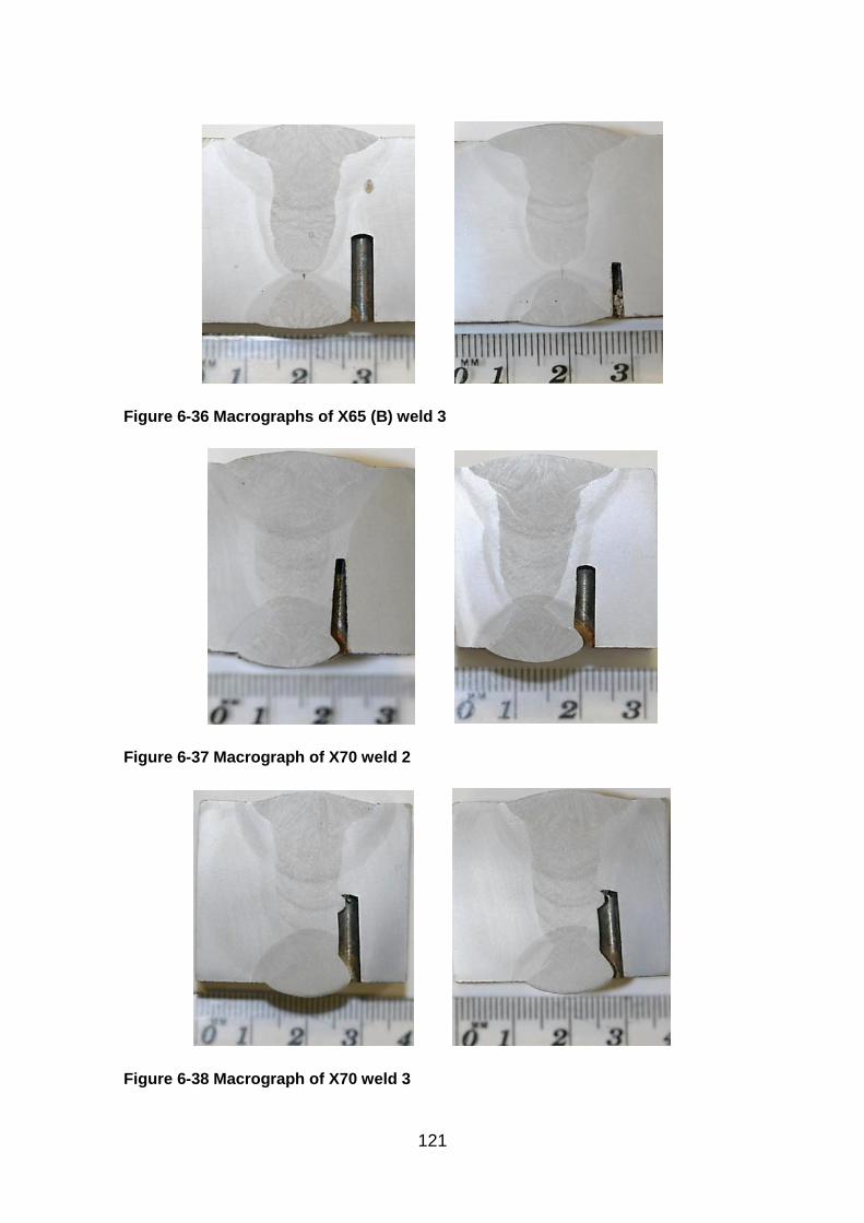
121

Figure 6-36 Macrographs of X65 (B) weld 3

Figure 6-37 Macrograph of X70 weld 2

Figure 6-38 Macrograph of X70 weld 3

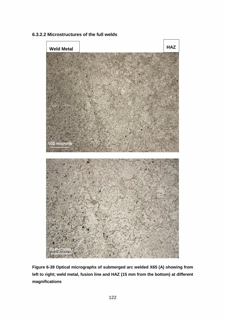
122

6.3.2.2 Microstructures of the full welds

Figure 6-39 Optical micrographs of submerged arc welded X65 (A) showing from

left to right; weld metal, fusion line and HAZ (15 mm from the bottom) at different

magnifications

Weld Metal HAZ

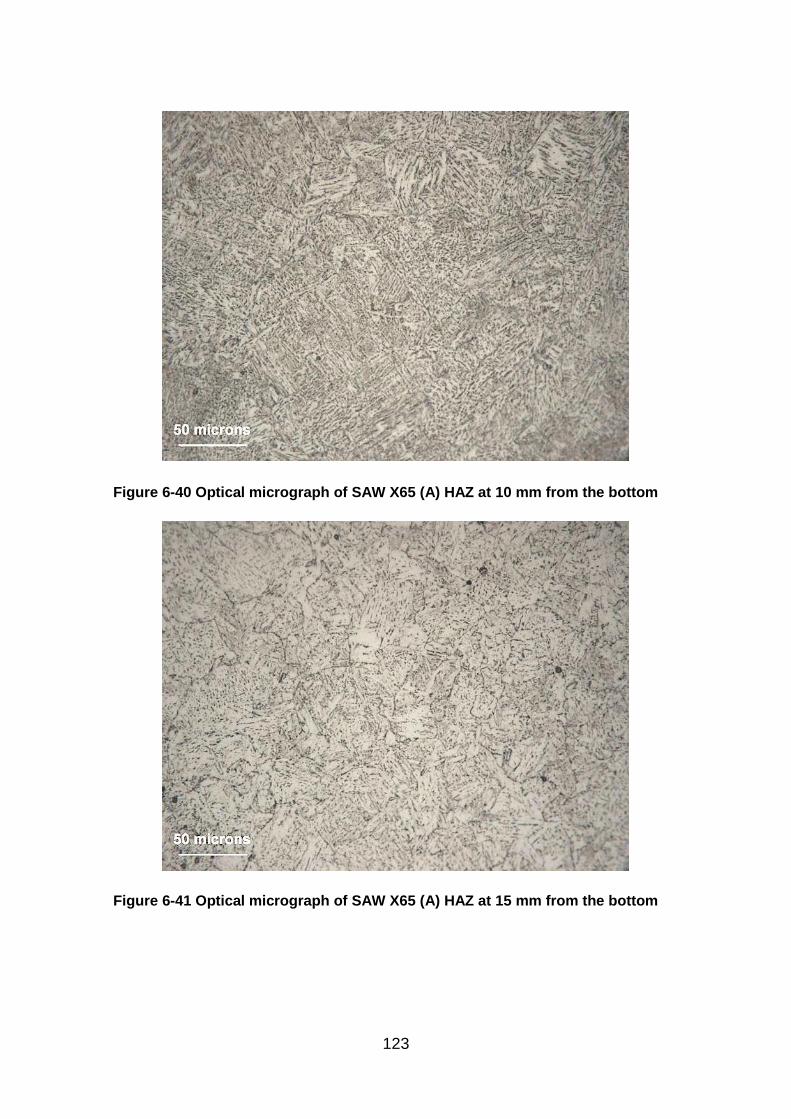
123

Figure 6-40 Optical micrograph of SAW X65 (A) HAZ at 10 mm from the bottom

Figure 6-41 Optical micrograph of SAW X65 (A) HAZ at 15 mm from the bottom

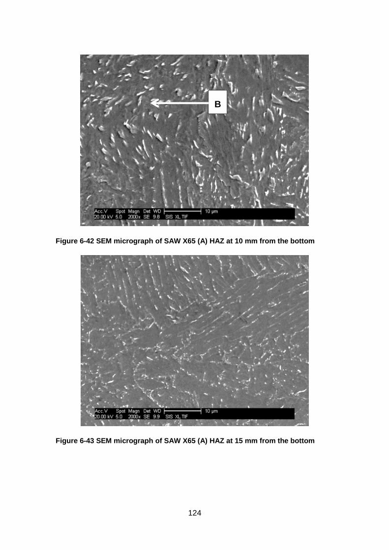
124

Figure 6-42 SEM micrograph of SAW X65 (A) HAZ at 10 mm from the bottom

Figure 6-43 SEM micrograph of SAW X65 (A) HAZ at 15 mm from the bottom

B

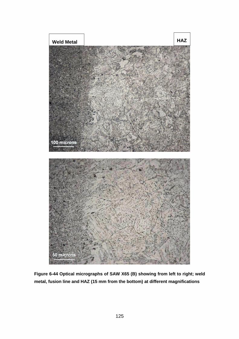
125

Figure 6-44 Optical micrographs of SAW X65 (B) showing from left to right; weld

metal, fusion line and HAZ (15 mm from the bottom) at different magnifications

Weld Metal HAZ

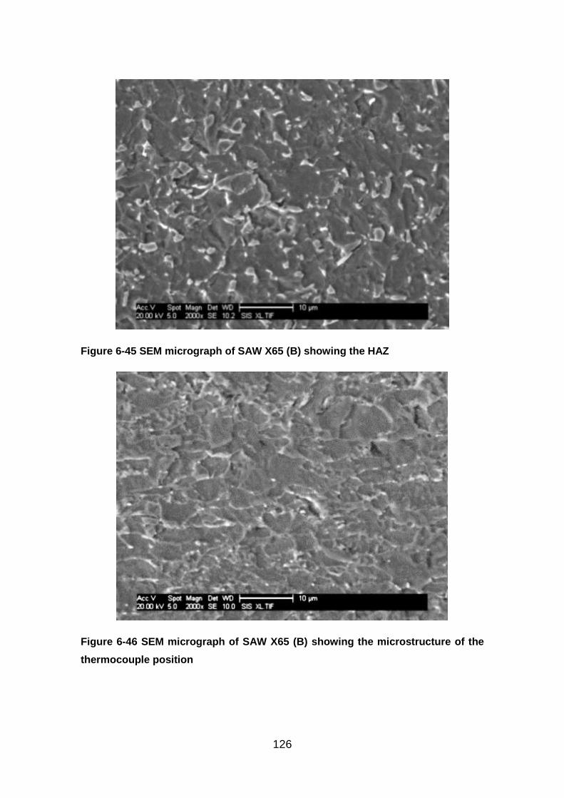
126

Figure 6-45 SEM micrograph of SAW X65 (B) showing the HAZ

Figure 6-46 SEM micrograph of SAW X65 (B) showing the microstructure of the

thermocouple position

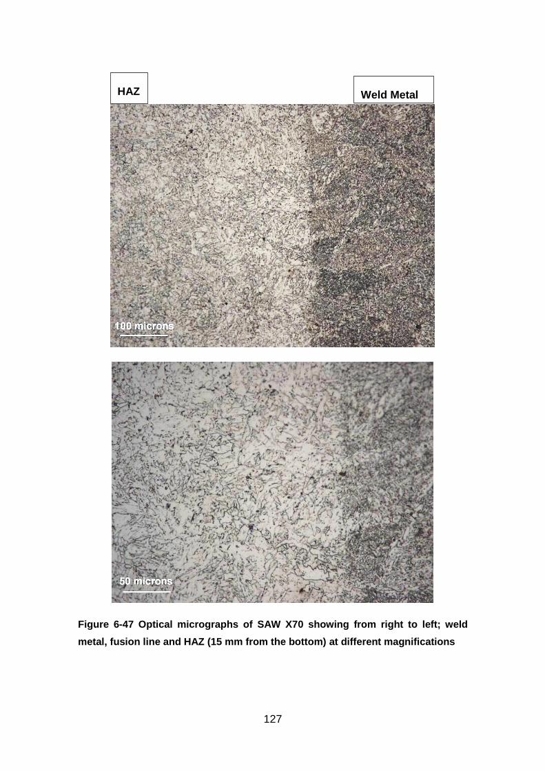
127

Figure 6-47 Optical micrographs of SAW X70 showing from right to left; weld

metal, fusion line and HAZ (15 mm from the bottom) at different magnifications

HAZ Weld Metal

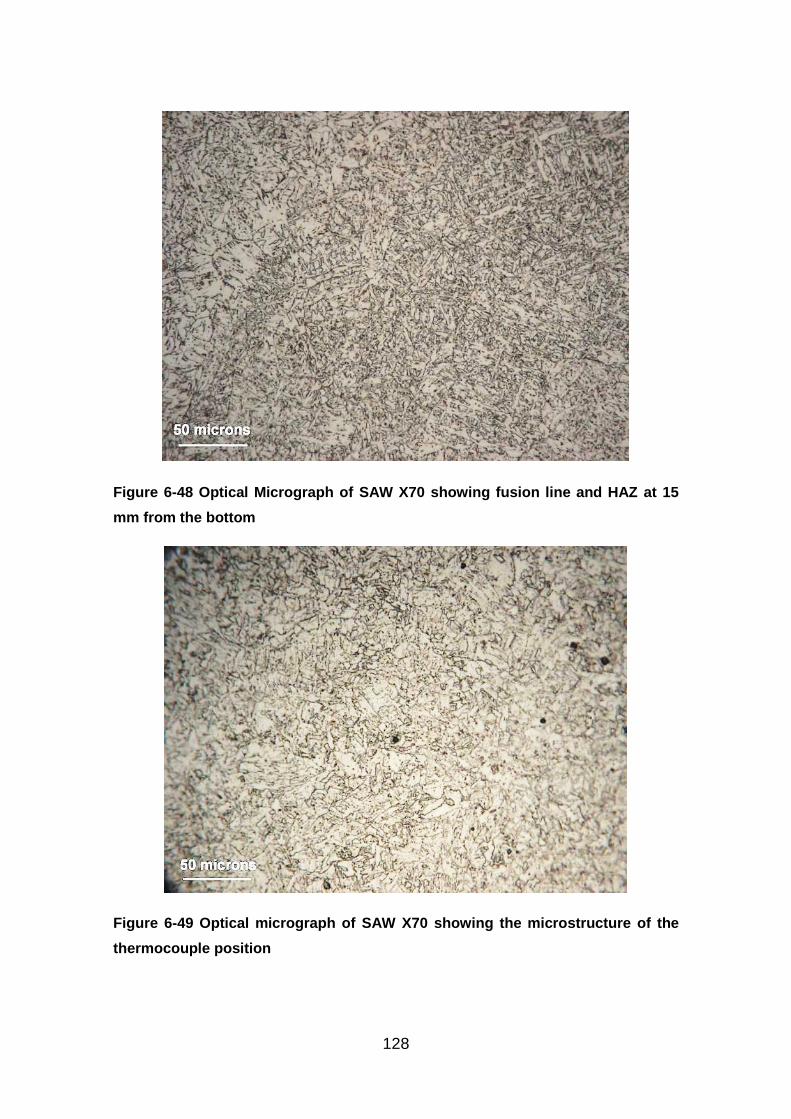
128

Figure 6-48 Optical Micrograph of SAW X70 showing fusion line and HAZ at 15

mm from the bottom

Figure 6-49 Optical micrograph of SAW X70 showing the microstructure of the

thermocouple position

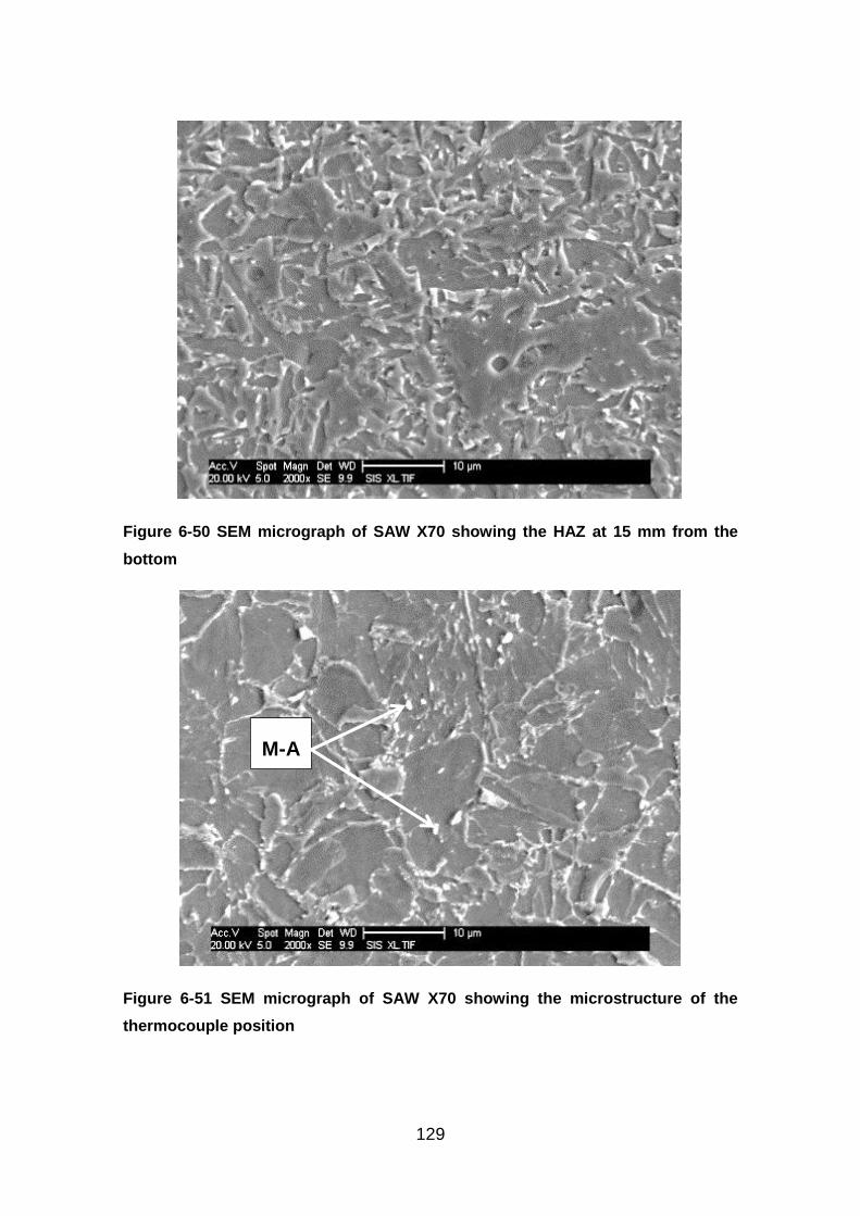
129

Figure 6-50 SEM micrograph of SAW X70 showing the HAZ at 15 mm from the

bottom

Figure 6-51 SEM micrograph of SAW X70 showing the microstructure of the

thermocouple position

M-A

130

6.3.2.3 Comparison between nital and LePèra etchants

Figure 6-52 Optical micrographs of X65 (A) SAW HAZ at 15 mm from the bottom,

showing (a) Nital etch and (b) LePèra etched

(a)

(b)

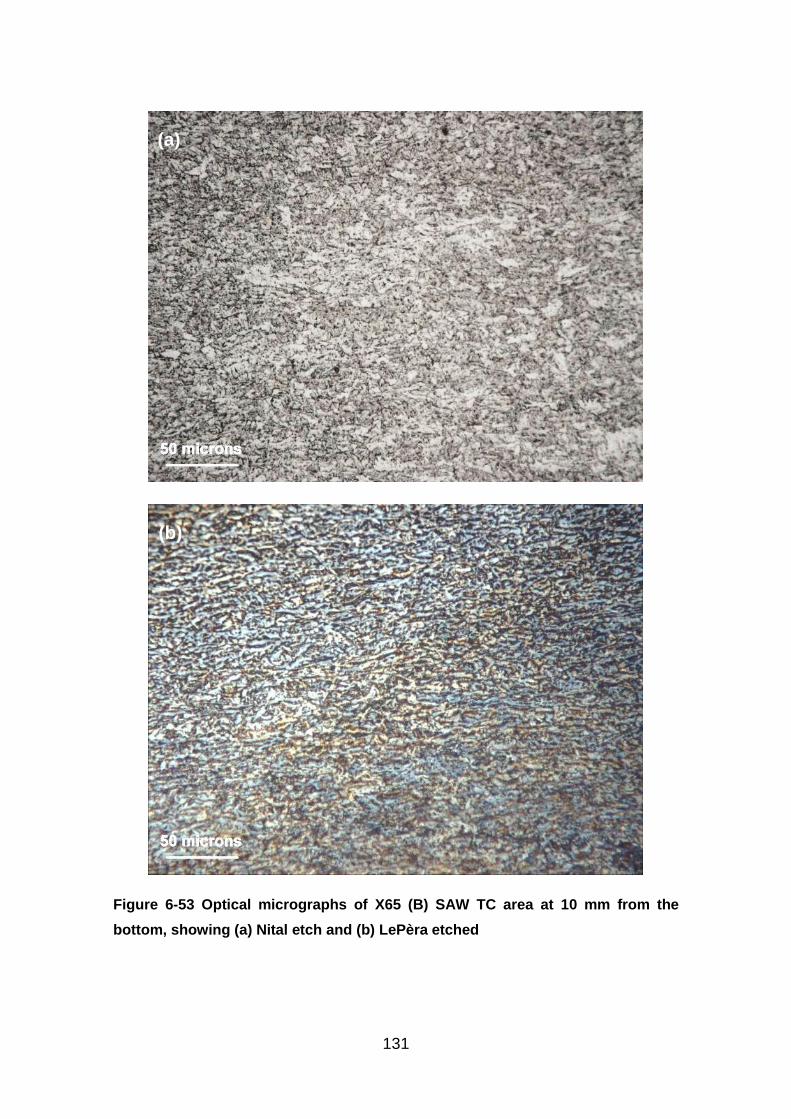
131

Figure 6-53 Optical micrographs of X65 (B) SAW TC area at 10 mm from the

bottom, showing (a) Nital etch and (b) LePèra etched

(b)

(a)

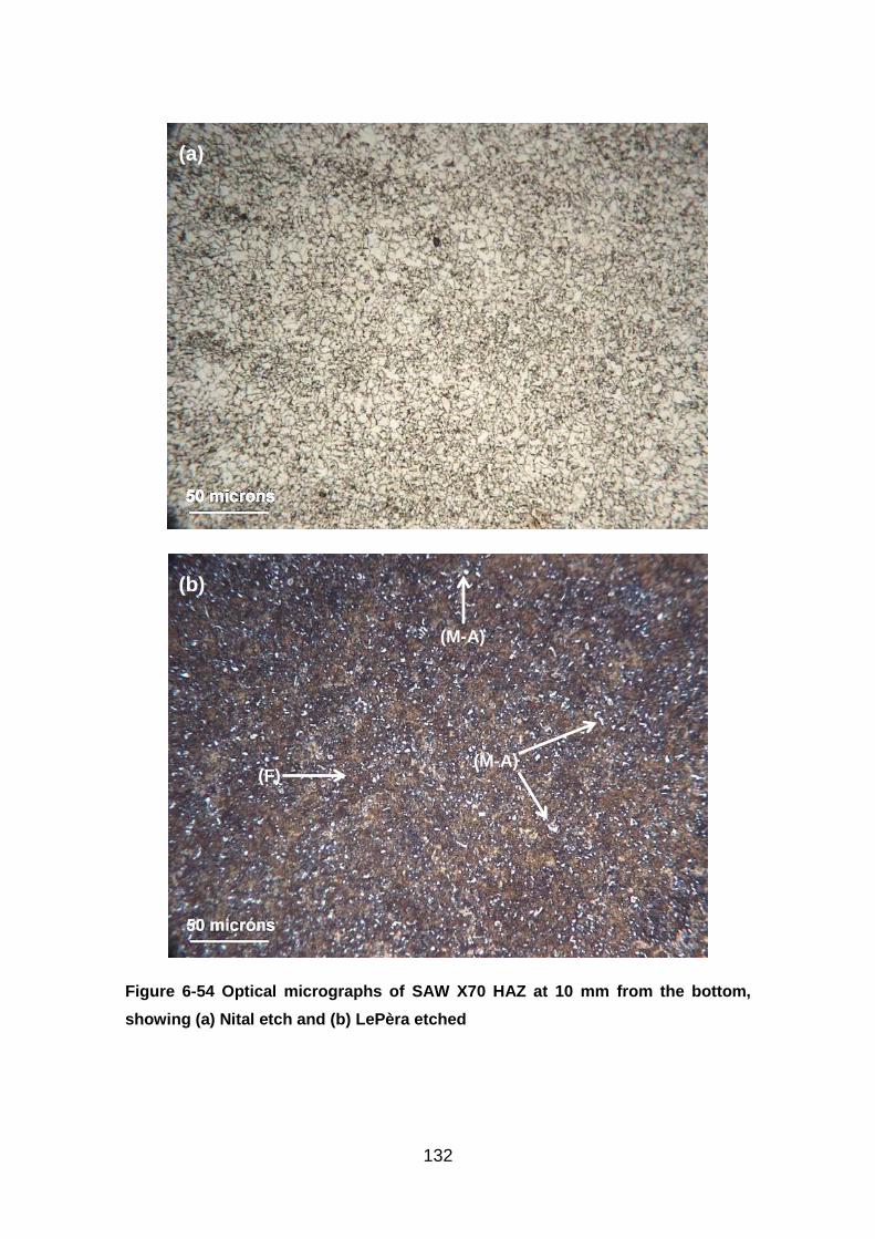
132

Figure 6-54 Optical micrographs of SAW X70 HAZ at 10 mm from the bottom,

showing (a) Nital etch and (b) LePèra etched

(a)

(b)

(F)

(M-A)

(M-A)

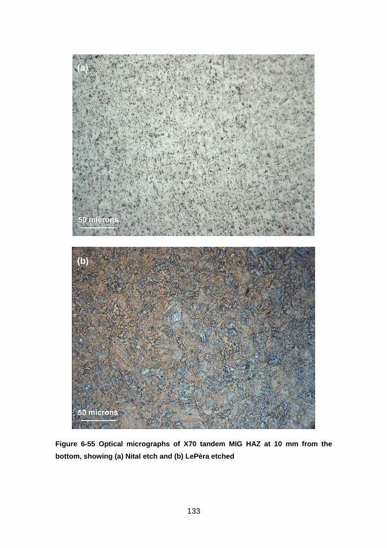
133

Figure 6-55 Optical micrographs of X70 tandem MIG HAZ at 10 mm from the

bottom, showing (a) Nital etch and (b) LePèra etched

(b)

(a)

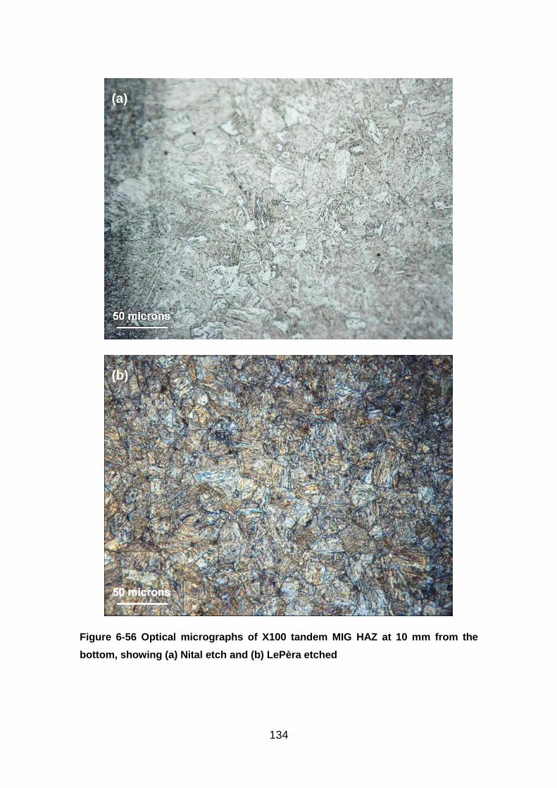
134

Figure 6-56 Optical micrographs of X100 tandem MIG HAZ at 10 mm from the

bottom, showing (a) Nital etch and (b) LePèra etched

(b)

(a)

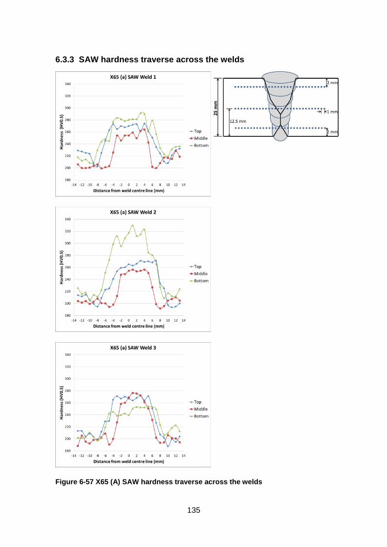
135

6.3.3 SAW hardness traverse across the welds

Figure 6-57 X65 (A) SAW hardness traverse across the welds

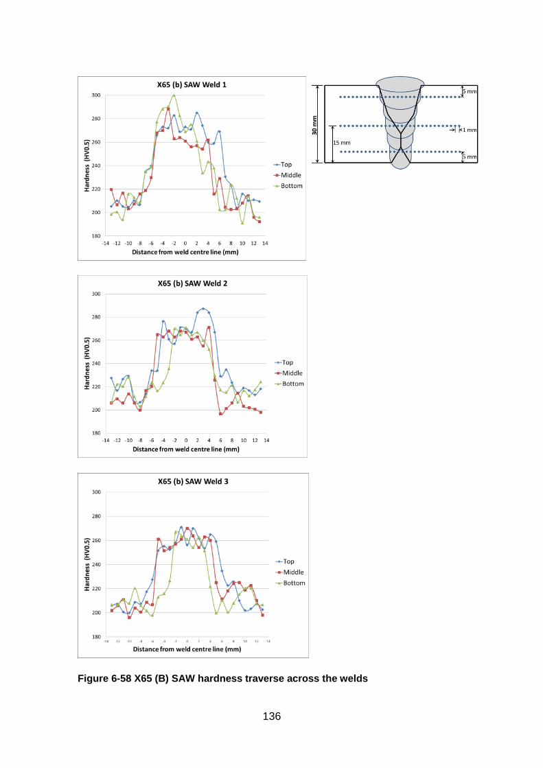
136

Figure 6-58 X65 (B) SAW hardness traverse across the welds

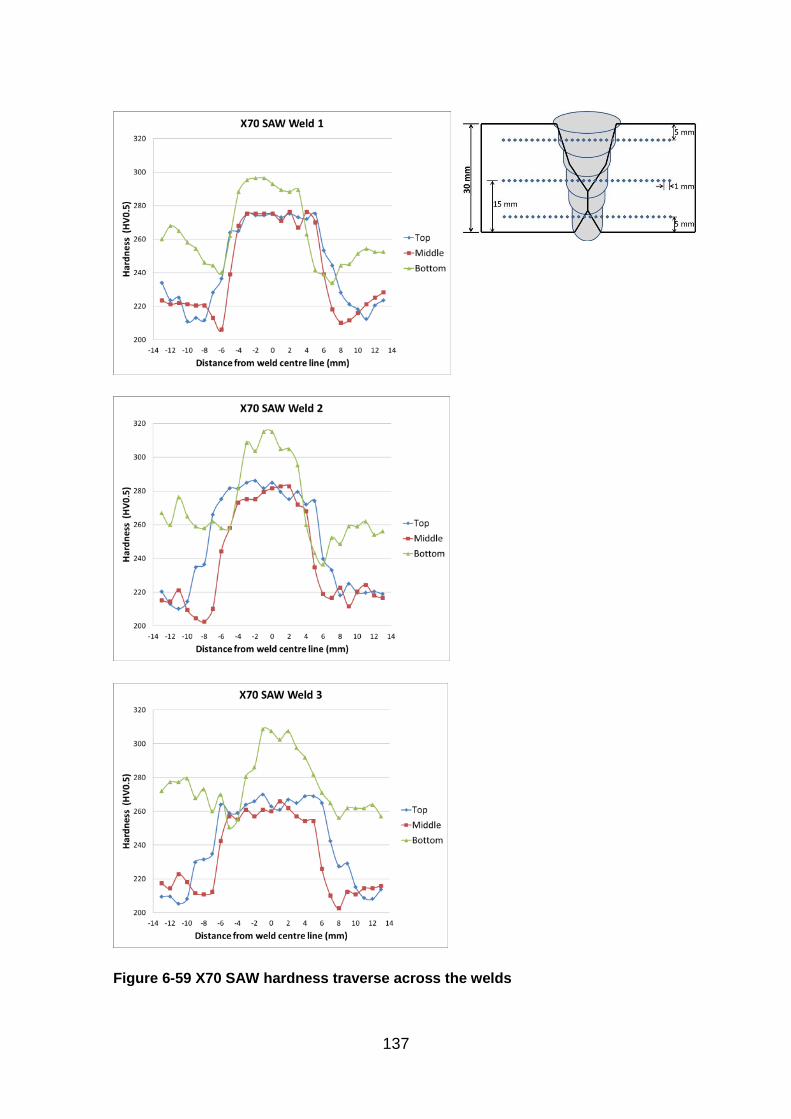
137

Figure 6-59 X70 SAW hardness traverse across the welds

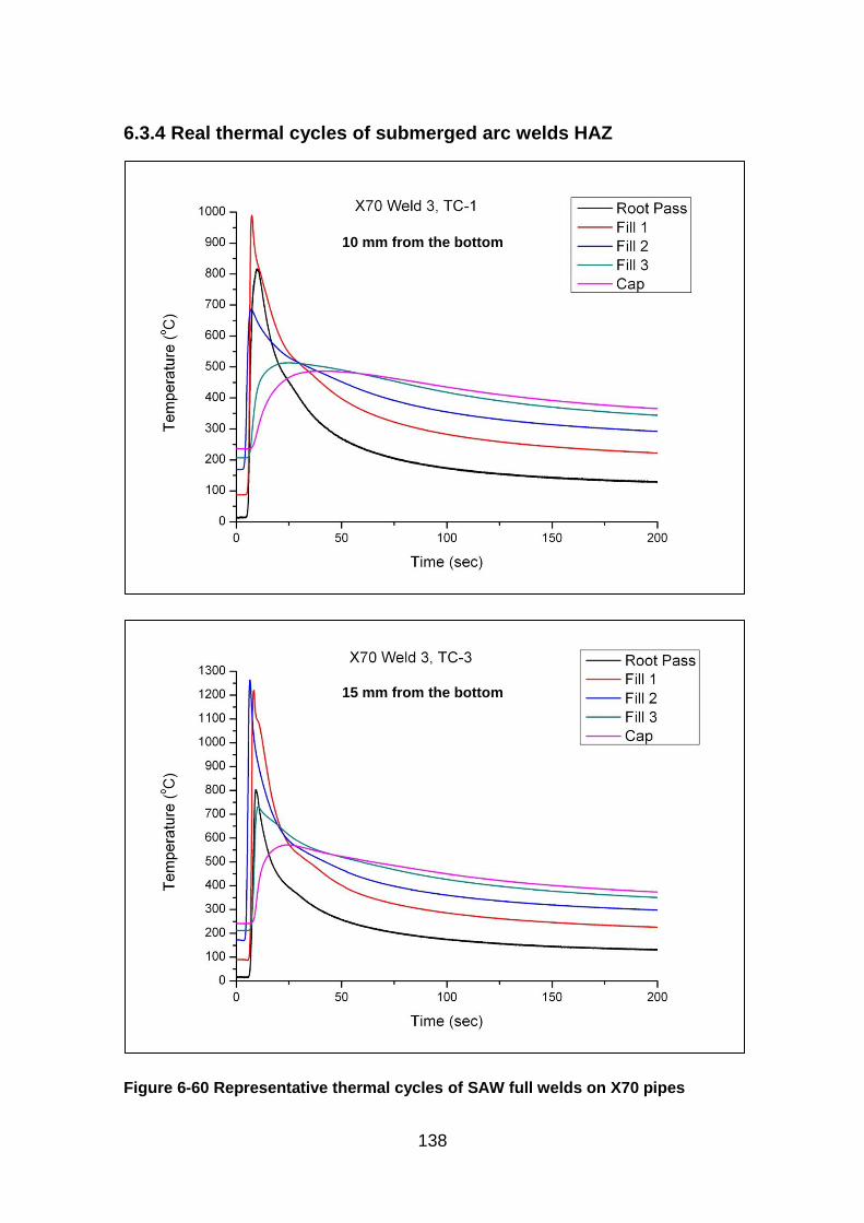
138

6.3.4 Real thermal cycles of submerged arc welds HAZ

Figure 6-60 Representative thermal cycles of SAW full welds on X70 pipes

10 mm from the bottom

15 mm from the bottom

139

6.3.5 Crack tip opening displacement test (CTOD) results

Table 6-4 CTOD results of the HAZ from selected welds

Weld Name HAZ CTOD (mm) Fracture Mode

SAW X65 (A) Weld 1 δ = 0.83 M

SAW X65 (A) Weld 3 δ = 0.88 M

SAW X65 (B) Weld 1 δ = 1.03 M(a)

SAW X65 (B) Weld 3 δ = 0.26 U(a)

SAW X70 Weld 1 δ = 0.098 C

SAW X70 Weld 2 δ = 0.69 U

(a) The pre-crack shape failed to satisfy the requirements of BS 7448-2, i.e. greater than 20%

variation in crack length and less than 1.3 mm minimum pre-crack length.

δ crack tip opening displacement (CTOD)

∆a Stable crack extension, including stretch zone width in mm

δc (C) critical δ at the onset of brittle crack extension when ∆a < 0.2 mm

δm (M) δ at the first attainment of maximum F (force) plateau for fully

plastic behaviour

δu (U) critical δ at the onset of brittle crack extension when ∆a ≥ 0.2 mm

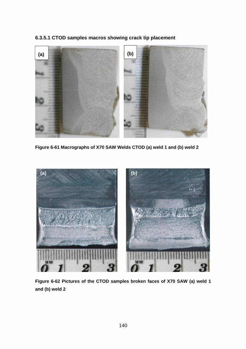
140

6.3.5.1 CTOD samples macros showing crack tip placement

Figure 6-61 Macrographs of X70 SAW Welds CTOD (a) weld 1 and (b) weld 2

Figure 6-62 Pictures of the CTOD samples broken faces of X70 SAW (a) weld 1

and (b) weld 2

(a) (b)

(a) (b)

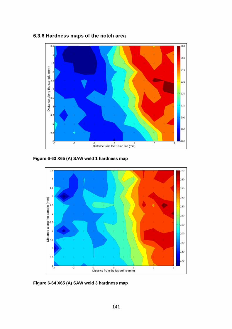
141

6.3.6 Hardness maps of the notch area

Figure 6-63 X65 (A) SAW weld 1 hardness map

Figure 6-64 X65 (A) SAW weld 3 hardness map

Distance from the fusion line (mm)

Dis

tance (

mm

)

-3 -2 -1 0 1 2 3

0.5

1

1.5

2

2.5

3

3.5

4

4.5

5

5.5

6 180

190

200

210

220

230

240

250

260

Distance from the fusion line (mm)

Dis

tance (

mm

)

-3 -2 -1 0 1 2 3

0.5

1

1.5

2

2.5

3

3.5

4

4.5

5

5.5

6

170

180

190

200

210

220

230

240

250

260

270

Dis

tance a

long the s

am

ple

(m

m)

Dis

tance a

long the s

am

ple

(m

m)

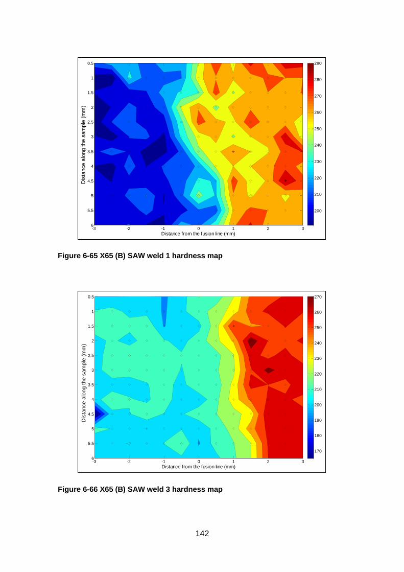
142

Figure 6-65 X65 (B) SAW weld 1 hardness map

Figure 6-66 X65 (B) SAW weld 3 hardness map

Distance from the fusion line (mm)

Dis

tance (

mm

)

-3 -2 -1 0 1 2 3

0.5

1

1.5

2

2.5

3

3.5

4

4.5

5

5.5

6

200

210

220

230

240

250

260

270

280

290

Distance from the fusion line (mm)

Dis

tance (

mm

)

-3 -2 -1 0 1 2 3

0.5

1

1.5

2

2.5

3

3.5

4

4.5

5

5.5

6

170

180

190

200

210

220

230

240

250

260

270

Dis

tance a

long the s

am

ple

(m

m)

Dis

tance a

long the s

am

ple

(m

m)

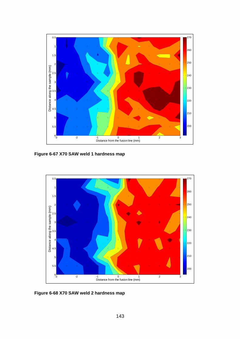
143

Figure 6-67 X70 SAW weld 1 hardness map

Figure 6-68 X70 SAW weld 2 hardness map

Distance from the fusion line (mm)

Dis

tance (

mm

)

-3 -2 -1 0 1 2 3

0.5

1

1.5

2

2.5

3

3.5

4

4.5

5

5.5

6

200

210

220

230

240

250

260

270

Distance from the fusion line (mm)

Dis

tance (

mm

)

-3 -2 -1 0 1 2 3

0.5

1

1.5

2

2.5

3

3.5

4

4.5

5

5.5

6

200

210

220

230

240

250

260

270

Dis

tance a

long the s

am

ple

(m

m)

Dis

tance a

long the s

am

ple

(m

m)

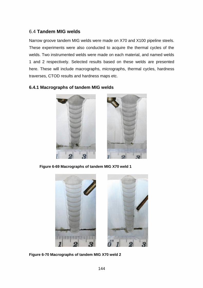
144

Tandem MIG welds 6.4

Narrow groove tandem MIG welds were made on X70 and X100 pipeline steels.

These experiments were also conducted to acquire the thermal cycles of the

welds. Two instrumented welds were made on each material, and named welds

1 and 2 respectively. Selected results based on these welds are presented

here. These will include macrographs, micrographs, thermal cycles, hardness

traverses, CTOD results and hardness maps etc.

6.4.1 Macrographs of tandem MIG welds

Figure 6-69 Macrographs of tandem MIG X70 weld 1

Figure 6-70 Macrographs of tandem MIG X70 weld 2

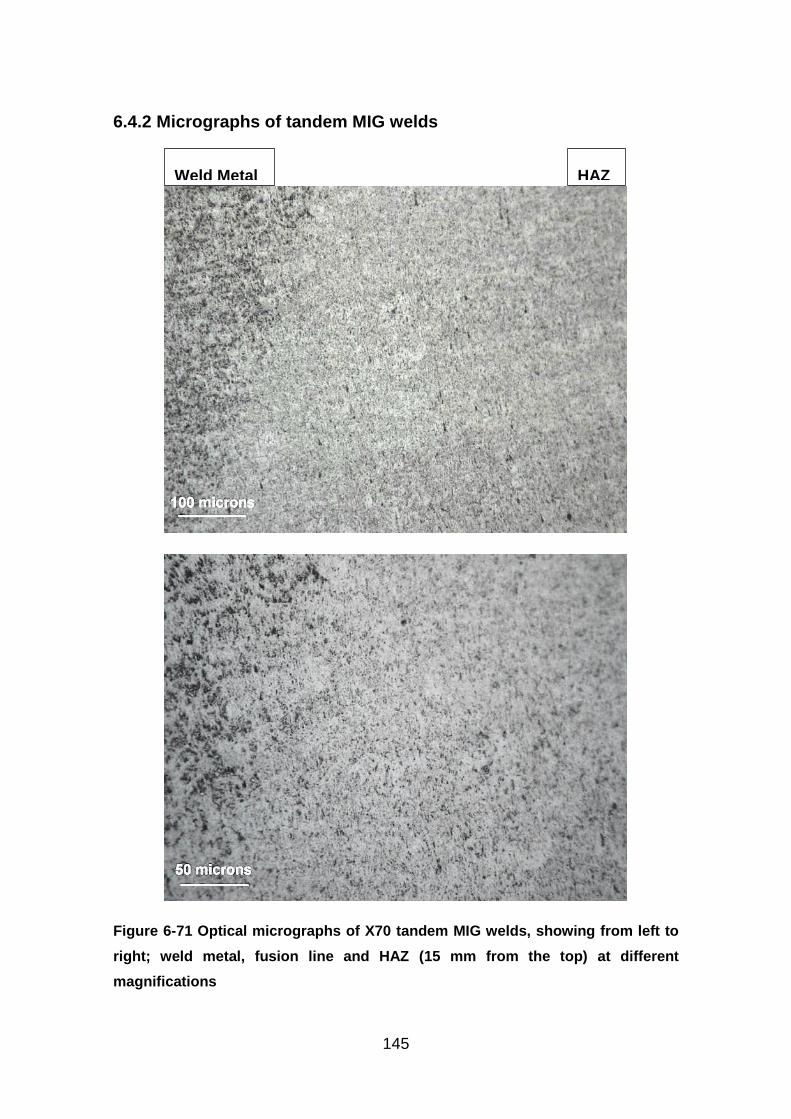
145

6.4.2 Micrographs of tandem MIG welds

Figure 6-71 Optical micrographs of X70 tandem MIG welds, showing from left to

right; weld metal, fusion line and HAZ (15 mm from the top) at different

magnifications

Weld Metal HAZ

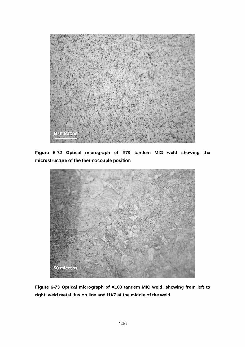
146

Figure 6-72 Optical micrograph of X70 tandem MIG weld showing the

microstructure of the thermocouple position

Figure 6-73 Optical micrograph of X100 tandem MIG weld, showing from left to

right; weld metal, fusion line and HAZ at the middle of the weld

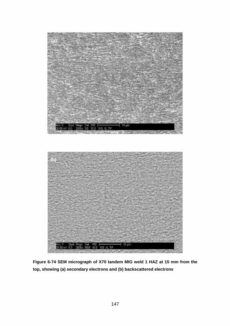
147

Figure 6-74 SEM micrograph of X70 tandem MIG weld 1 HAZ at 15 mm from the

top, showing (a) secondary electrons and (b) backscattered electrons

(a)

(b)

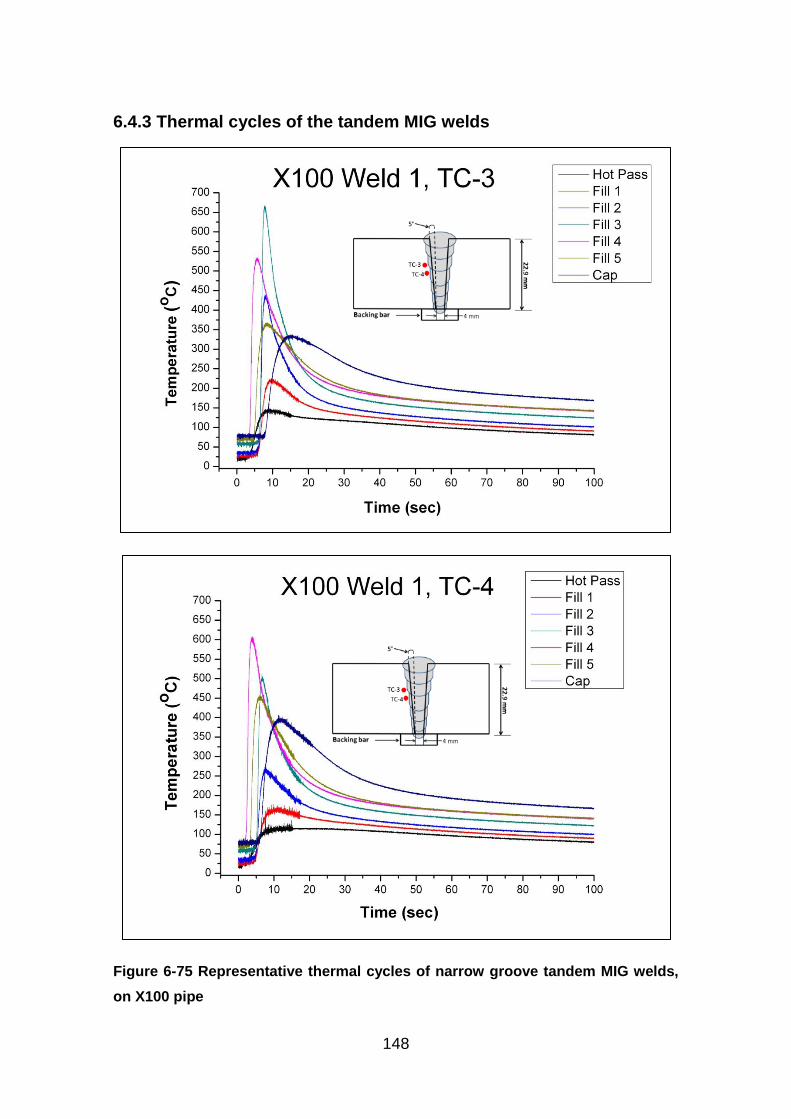
148

6.4.3 Thermal cycles of the tandem MIG welds

Figure 6-75 Representative thermal cycles of narrow groove tandem MIG welds,

on X100 pipe

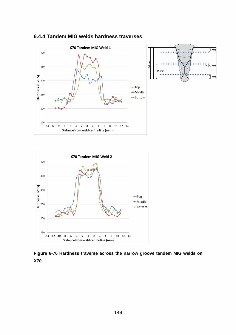
149

6.4.4 Tandem MIG welds hardness traverses

Figure 6-76 Hardness traverse across the narrow groove tandem MIG welds on

X70

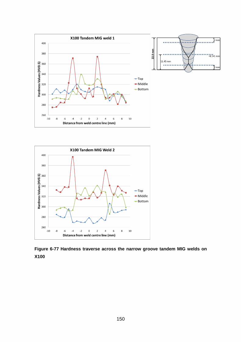
150

Figure 6-77 Hardness traverse across the narrow groove tandem MIG welds on

X100

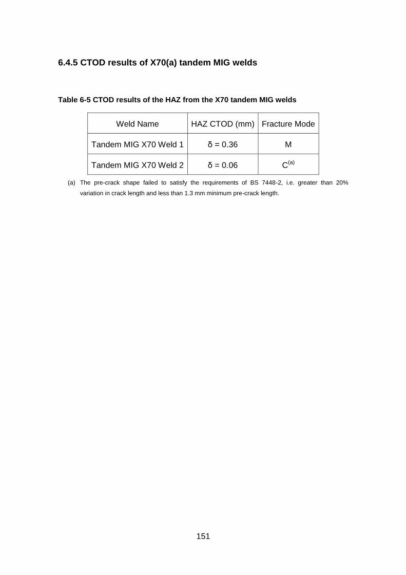
151

6.4.5 CTOD results of X70(a) tandem MIG welds

Table 6-5 CTOD results of the HAZ from the X70 tandem MIG welds

Weld Name HAZ CTOD (mm) Fracture Mode

Tandem MIG X70 Weld 1 δ = 0.36 M

Tandem MIG X70 Weld 2 δ = 0.06 C(a)

(a) The pre-crack shape failed to satisfy the requirements of BS 7448-2, i.e. greater than 20%

variation in crack length and less than 1.3 mm minimum pre-crack length.

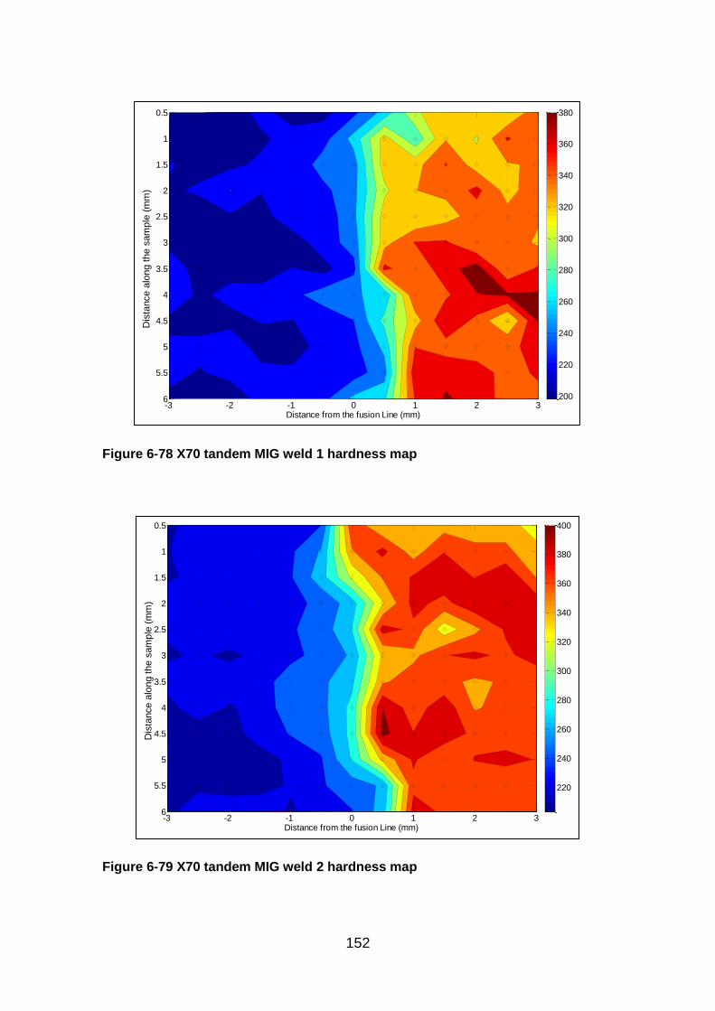
152

Figure 6-78 X70 tandem MIG weld 1 hardness map

Figure 6-79 X70 tandem MIG weld 2 hardness map

Distance from the fusion Line (mm)

Dis

tance (

mm

)

-3 -2 -1 0 1 2 3

0.5

1

1.5

2

2.5

3

3.5

4

4.5

5

5.5

6 200

220

240

260

280

300

320

340

360

380

Distance from the fusion Line (mm)

Dis

tance (

mm

)

-3 -2 -1 0 1 2 3

0.5

1

1.5

2

2.5

3

3.5

4

4.5

5

5.5

6

220

240

260

280

300

320

340

360

380

400

Dis

tance a

long the s

am

ple

(m

m)

Dis

tance a

long the s

am

ple

(m

m)

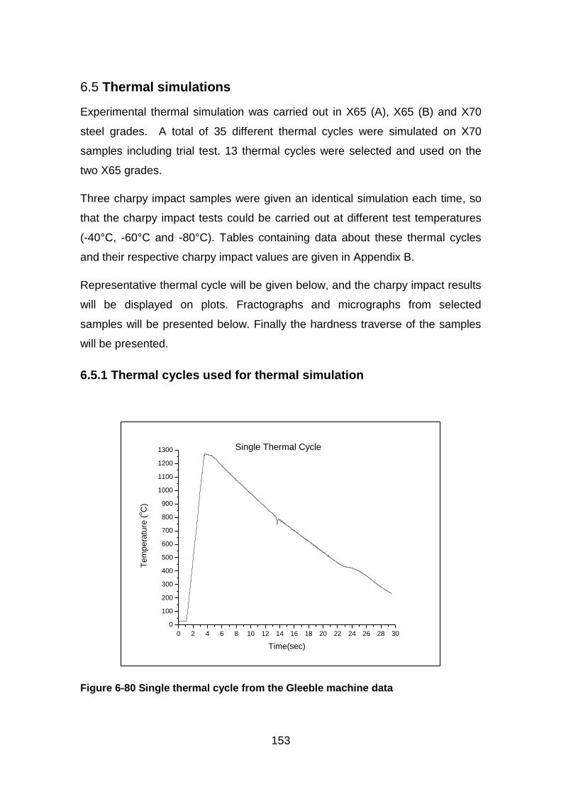
153

Thermal simulations 6.5

Experimental thermal simulation was carried out in X65 (A), X65 (B) and X70

steel grades. A total of 35 different thermal cycles were simulated on X70

samples including trial test. 13 thermal cycles were selected and used on the

two X65 grades.

Three charpy impact samples were given an identical simulation each time, so

that the charpy impact tests could be carried out at different test temperatures

(-40°C, -60°C and -80°C). Tables containing data about these thermal cycles

and their respective charpy impact values are given in Appendix B.

Representative thermal cycle will be given below, and the charpy impact results

will be displayed on plots. Fractographs and micrographs from selected

samples will be presented below. Finally the hardness traverse of the samples

will be presented.

6.5.1 Thermal cycles used for thermal simulation

Figure 6-80 Single thermal cycle from the Gleeble machine data

0 2 4 6 8 10 12 14 16 18 20 22 24 26 28 30

0

100

200

300

400

500

600

700

800

900

1000

1100

1200

1300 Single Thermal Cycle

Te

mp

era

ture

(oC

)

Time(sec)

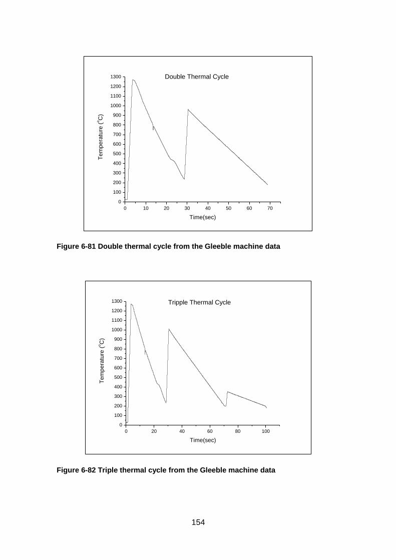
154

Figure 6-81 Double thermal cycle from the Gleeble machine data

Figure 6-82 Triple thermal cycle from the Gleeble machine data

0 10 20 30 40 50 60 70

0

100

200

300

400

500

600

700

800

900

1000

1100

1200

1300 Double Thermal Cycle

Te

mp

era

ture

(oC

)

Time(sec)

0 20 40 60 80 100

0

100

200

300

400

500

600

700

800

900

1000

1100

1200

1300 Tripple Thermal Cycle

Te

mp

era

ture

(oC

)

Time(sec)

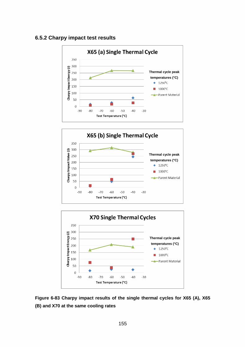
155

6.5.2 Charpy impact test results

Figure 6-83 Charpy impact results of the single thermal cycles for X65 (A), X65

(B) and X70 at the same cooling rates

Thermal cycle peak

temperatures (°C)

Thermal cycle peak

temperatures (°C)

Thermal cycle peak

temperatures (°C)

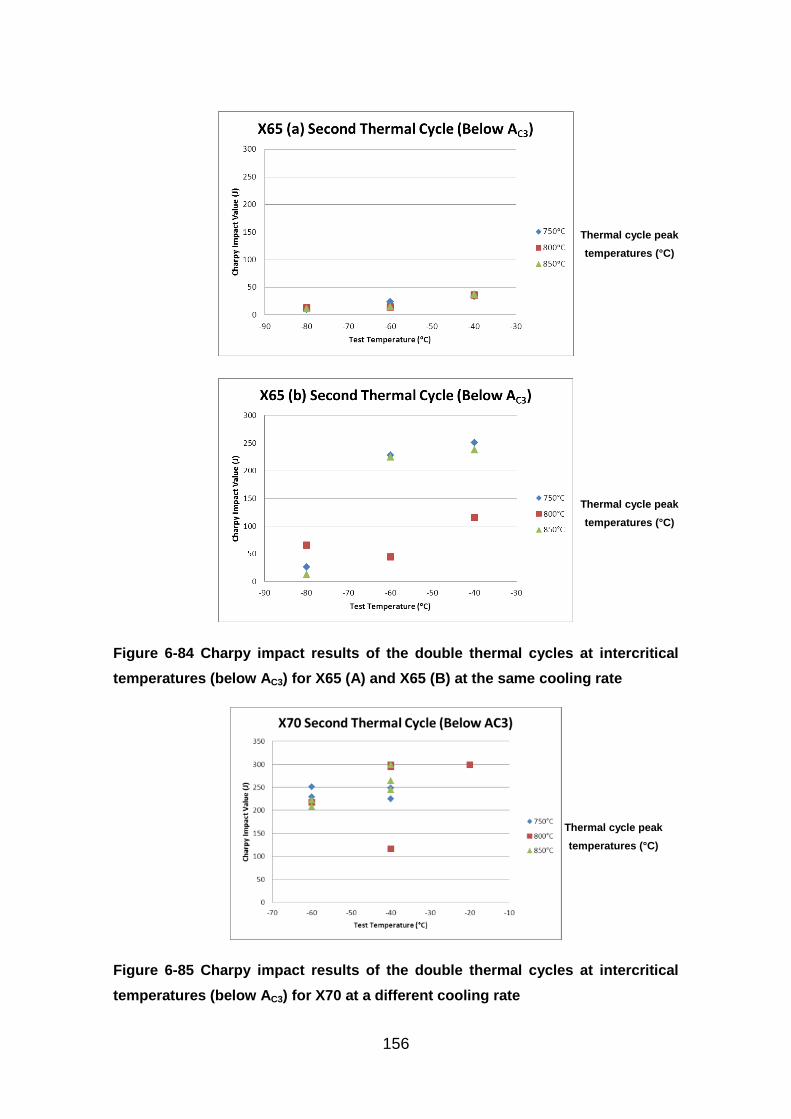
156

Figure 6-84 Charpy impact results of the double thermal cycles at intercritical

temperatures (below AC3) for X65 (A) and X65 (B) at the same cooling rate

Figure 6-85 Charpy impact results of the double thermal cycles at intercritical

temperatures (below AC3) for X70 at a different cooling rate

Thermal cycle peak

temperatures (°C)

Thermal cycle peak

temperatures (°C)

Thermal cycle peak

temperatures (°C)

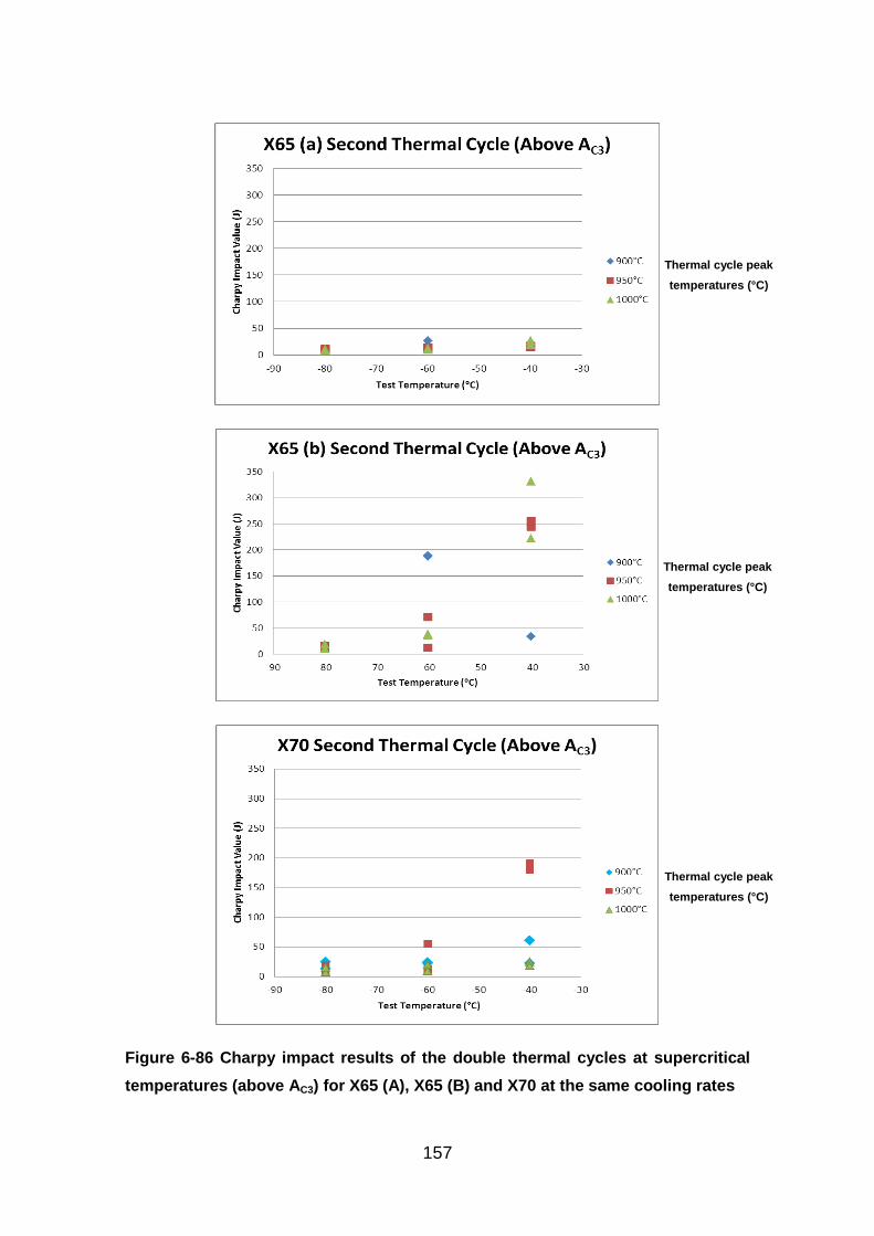
157

Figure 6-86 Charpy impact results of the double thermal cycles at supercritical

temperatures (above AC3) for X65 (A), X65 (B) and X70 at the same cooling rates

Thermal cycle peak

temperatures (°C)

Thermal cycle peak

temperatures (°C)

Thermal cycle peak

temperatures (°C)

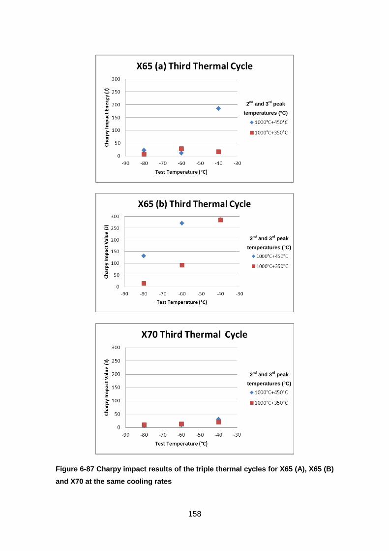
158

Figure 6-87 Charpy impact results of the triple thermal cycles for X65 (A), X65 (B)

and X70 at the same cooling rates

2nd

and 3rd

peak

temperatures (°C)

2nd

and 3rd

peak

temperatures (°C)

2nd

and 3rd

peak

temperatures (°C)

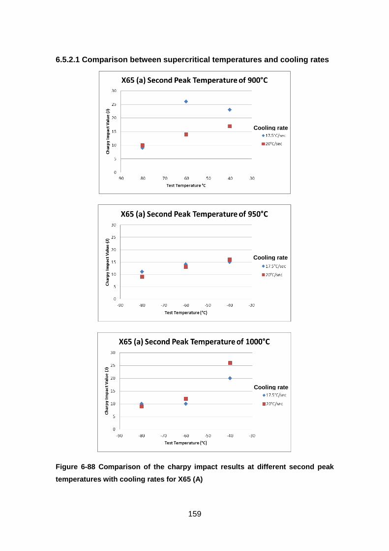
159

6.5.2.1 Comparison between supercritical temperatures and cooling rates

Figure 6-88 Comparison of the charpy impact results at different second peak

temperatures with cooling rates for X65 (A)

Cooling rate

Cooling rate

Cooling rate

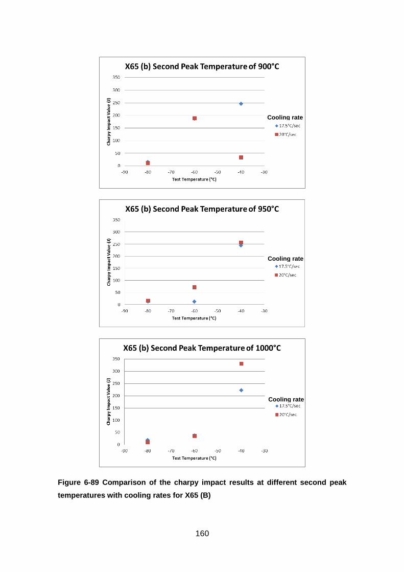
160

Figure 6-89 Comparison of the charpy impact results at different second peak

temperatures with cooling rates for X65 (B)

Cooling rate

Cooling rate

Cooling rate

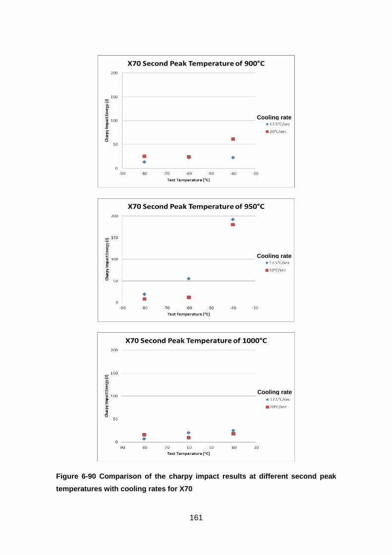
161

Figure 6-90 Comparison of the charpy impact results at different second peak

temperatures with cooling rates for X70

Cooling rate

Cooling rate

Cooling rate

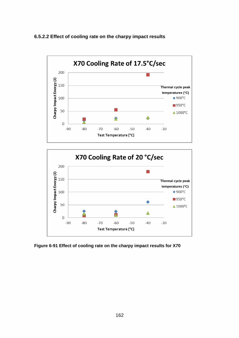
162

6.5.2.2 Effect of cooling rate on the charpy impact results

Figure 6-91 Effect of cooling rate on the charpy impact results for X70

Thermal cycle peak

temperatures (°C)

Thermal cycle peak

temperatures (°C)

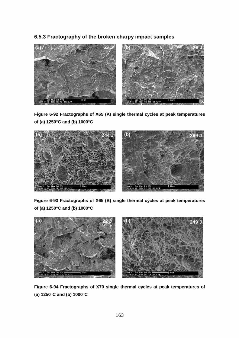
163

6.5.3 Fractography of the broken charpy impact samples

Figure 6-92 Fractographs of X65 (A) single thermal cycles at peak temperatures

of (a) 1250°C and (b) 1000°C

Figure 6-93 Fractographs of X65 (B) single thermal cycles at peak temperatures

of (a) 1250°C and (b) 1000°C

Figure 6-94 Fractographs of X70 single thermal cycles at peak temperatures of

(a) 1250°C and (b) 1000°C

(a) (b)

(b) (a)

(b) (a)

26 J

22 J

244 J

63 J

249 J

269 J

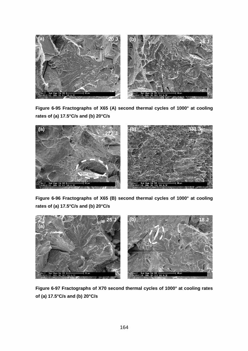
164

Figure 6-95 Fractographs of X65 (A) second thermal cycles of 1000° at cooling

rates of (a) 17.5°C/s and (b) 20°C/s

Figure 6-96 Fractographs of X65 (B) second thermal cycles of 1000° at cooling

rates of (a) 17.5°C/s and (b) 20°C/s

Figure 6-97 Fractographs of X70 second thermal cycles of 1000° at cooling rates

of (a) 17.5°C/s and (b) 20°C/s

(a) (b)

(b) (a)

(b)

(a)

20 J 26 J

331 J 222 J

25 J 18 J

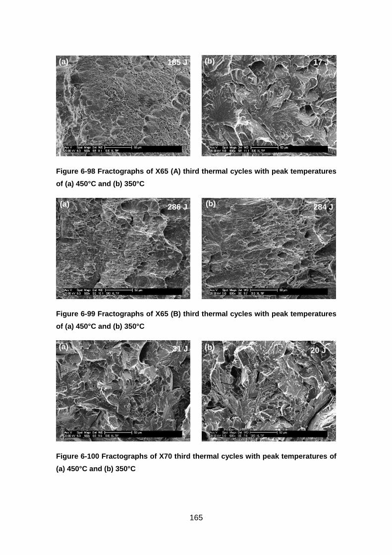
165

Figure 6-98 Fractographs of X65 (A) third thermal cycles with peak temperatures

of (a) 450°C and (b) 350°C

Figure 6-99 Fractographs of X65 (B) third thermal cycles with peak temperatures

of (a) 450°C and (b) 350°C

Figure 6-100 Fractographs of X70 third thermal cycles with peak temperatures of

(a) 450°C and (b) 350°C

(a)

(b) (a)

(b)

(b)

(a) 286 J

17 J 185 J

31 J 20 J

284 J

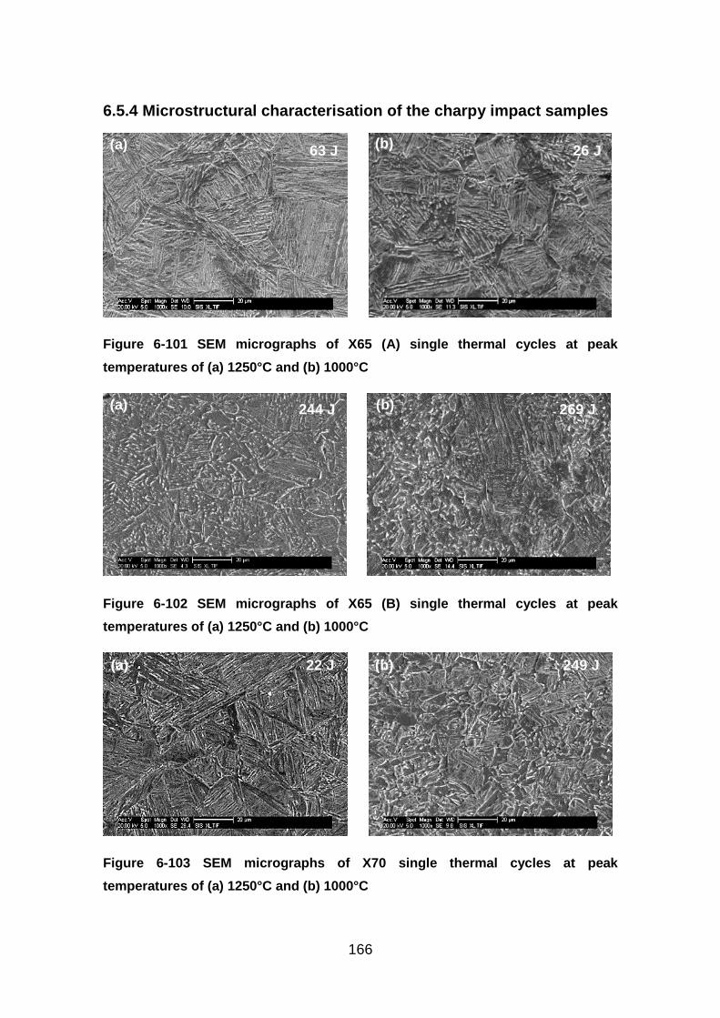
166

6.5.4 Microstructural characterisation of the charpy impact samples

Figure 6-101 SEM micrographs of X65 (A) single thermal cycles at peak

temperatures of (a) 1250°C and (b) 1000°C

Figure 6-102 SEM micrographs of X65 (B) single thermal cycles at peak

temperatures of (a) 1250°C and (b) 1000°C

Figure 6-103 SEM micrographs of X70 single thermal cycles at peak

temperatures of (a) 1250°C and (b) 1000°C

(b) (a)

(a)

(a) (b)

(b) 244 J 269 J

22 J 249 J

63 J 26 J

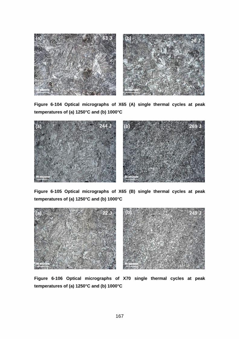
167

Figure 6-104 Optical micrographs of X65 (A) single thermal cycles at peak

temperatures of (a) 1250°C and (b) 1000°C

Figure 6-105 Optical micrographs of X65 (B) single thermal cycles at peak

temperatures of (a) 1250°C and (b) 1000°C

Figure 6-106 Optical micrographs of X70 single thermal cycles at peak

temperatures of (a) 1250°C and (b) 1000°C

(a)

(a)

(a) (b)

(b)

(b)

22 J 249 J

244 J

63 J

269 J

26 J

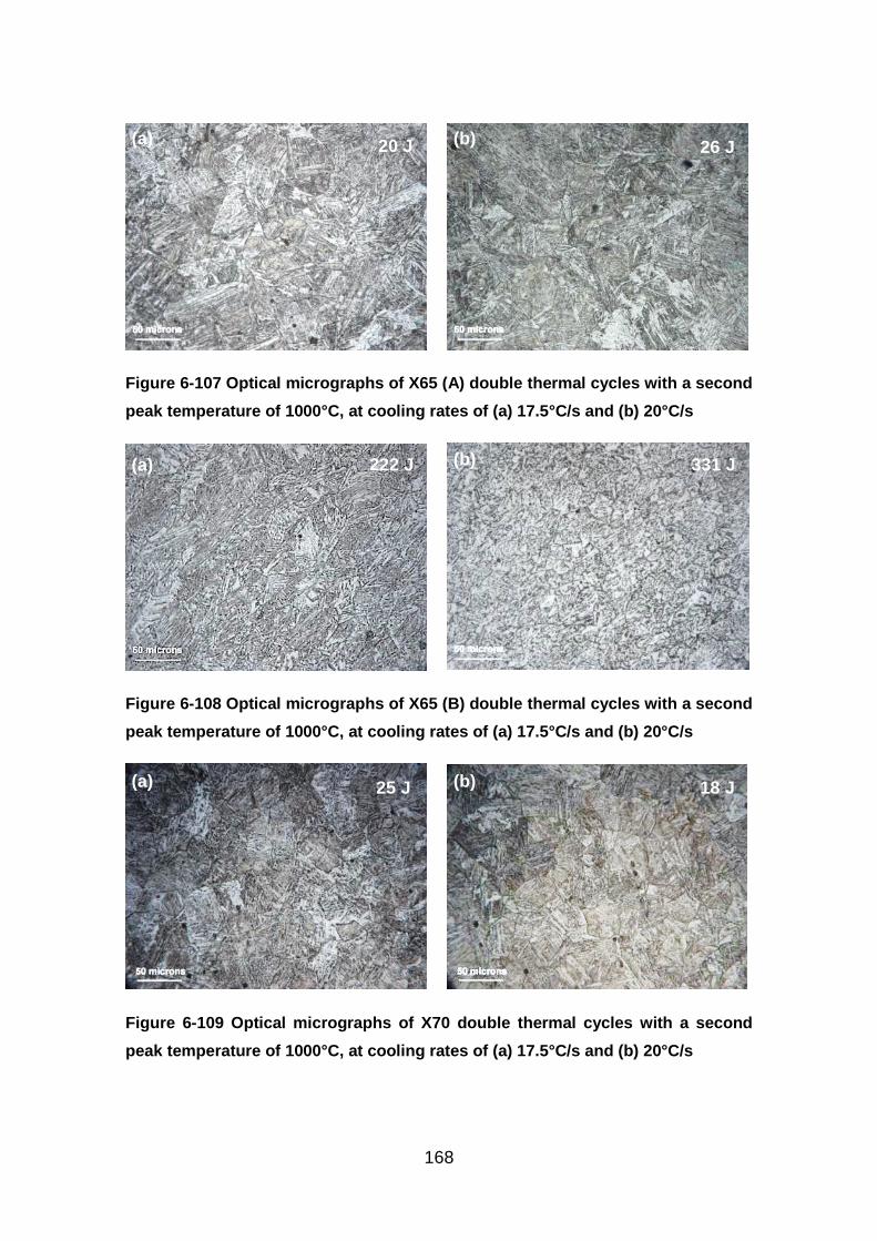
168

Figure 6-107 Optical micrographs of X65 (A) double thermal cycles with a second

peak temperature of 1000°C, at cooling rates of (a) 17.5°C/s and (b) 20°C/s

Figure 6-108 Optical micrographs of X65 (B) double thermal cycles with a second

peak temperature of 1000°C, at cooling rates of (a) 17.5°C/s and (b) 20°C/s

Figure 6-109 Optical micrographs of X70 double thermal cycles with a second

peak temperature of 1000°C, at cooling rates of (a) 17.5°C/s and (b) 20°C/s

(a)

(a)

(a)

(b)

(b)

(b)

331 J

20 J 26 J

18 J 25 J

222 J

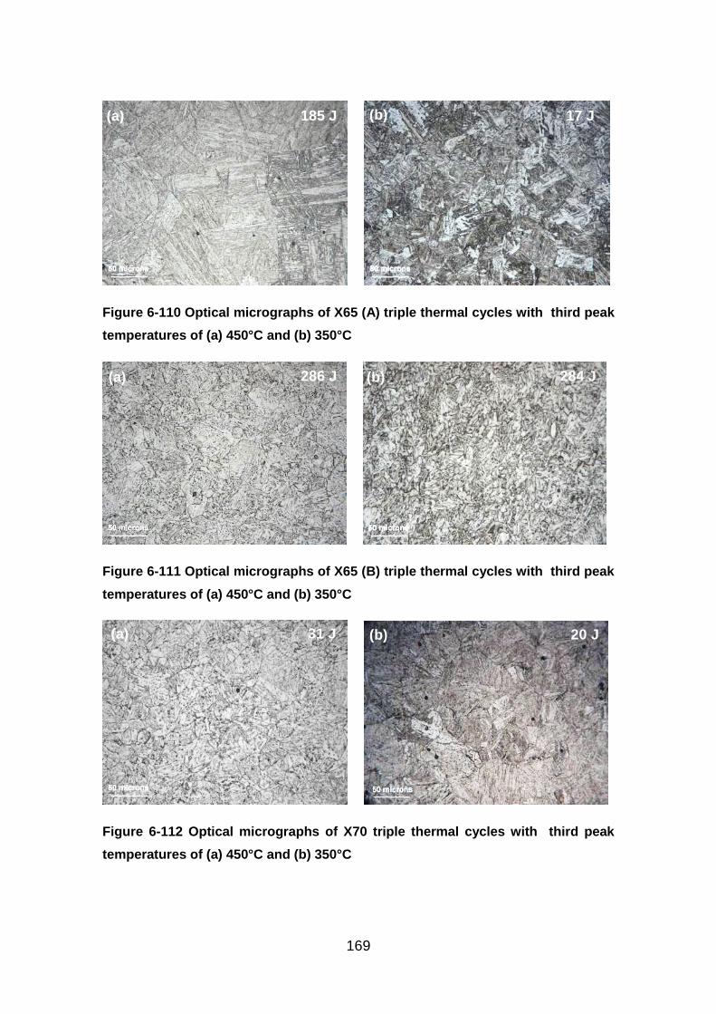
169

Figure 6-110 Optical micrographs of X65 (A) triple thermal cycles with third peak

temperatures of (a) 450°C and (b) 350°C

Figure 6-111 Optical micrographs of X65 (B) triple thermal cycles with third peak

temperatures of (a) 450°C and (b) 350°C

Figure 6-112 Optical micrographs of X70 triple thermal cycles with third peak

temperatures of (a) 450°C and (b) 350°C

(a)

(a)

(a)

(b)

(b)

(b)

284 J 286 J

185 J

31 J 20 J

17 J

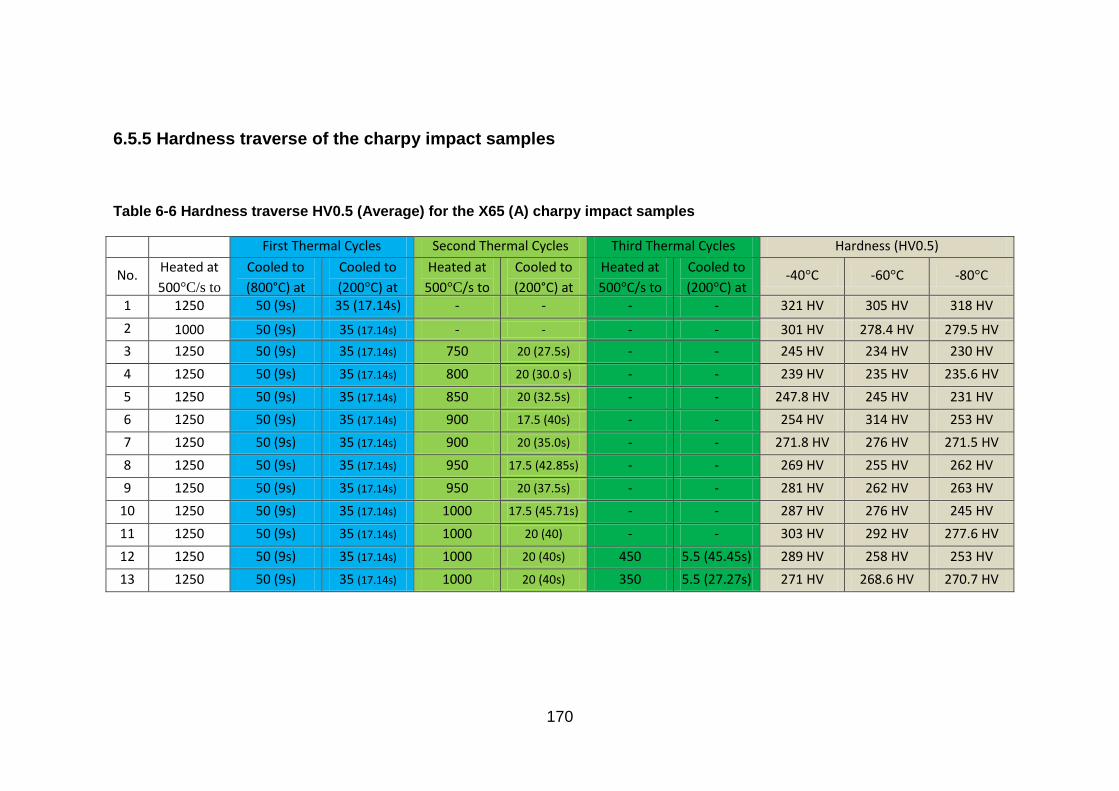
170

6.5.5 Hardness traverse of the charpy impact samples

Table 6-6 Hardness traverse HV0.5 (Average) for the X65 (A) charpy impact samples

First Thermal Cycles Second Thermal Cycles Third Thermal Cycles Hardness (HV0.5)

No. Heated at

500°C/s to

Cooled to

(800°C) at

°C/s

Cooled to

(200°C) at

°C/s

Heated at

500°C/s to

Cooled to

(200°C) at

°C/s

Heated at

500°C/s to

Cooled to

(200°C) at

°C/s

-40°C -60°C -80°C

1 1250 50 (9s) 35 (17.14s) - - - - 321 HV 305 HV 318 HV

2 1000 50 (9s) 35 (17.14s) - - - - 301 HV 278.4 HV 279.5 HV

3 1250 50 (9s) 35 (17.14s) 750 20 (27.5s) - - 245 HV 234 HV 230 HV

4 1250 50 (9s) 35 (17.14s) 800 20 (30.0 s) - - 239 HV 235 HV 235.6 HV

5 1250 50 (9s) 35 (17.14s) 850 20 (32.5s) - - 247.8 HV 245 HV 231 HV

6 1250 50 (9s) 35 (17.14s) 900 17.5 (40s) - - 254 HV 314 HV 253 HV

7 1250 50 (9s) 35 (17.14s) 900 20 (35.0s) - - 271.8 HV 276 HV 271.5 HV

8 1250 50 (9s) 35 (17.14s) 950 17.5 (42.85s) - - 269 HV 255 HV 262 HV

9 1250 50 (9s) 35 (17.14s) 950 20 (37.5s) - - 281 HV 262 HV 263 HV

10 1250 50 (9s) 35 (17.14s) 1000 17.5 (45.71s) - - 287 HV 276 HV 245 HV

11 1250 50 (9s) 35 (17.14s) 1000 20 (40) - - 303 HV 292 HV 277.6 HV

12 1250 50 (9s) 35 (17.14s) 1000 20 (40s) 450 5.5 (45.45s) 289 HV 258 HV 253 HV

13 1250 50 (9s) 35 (17.14s) 1000 20 (40s) 350 5.5 (27.27s) 271 HV 268.6 HV 270.7 HV

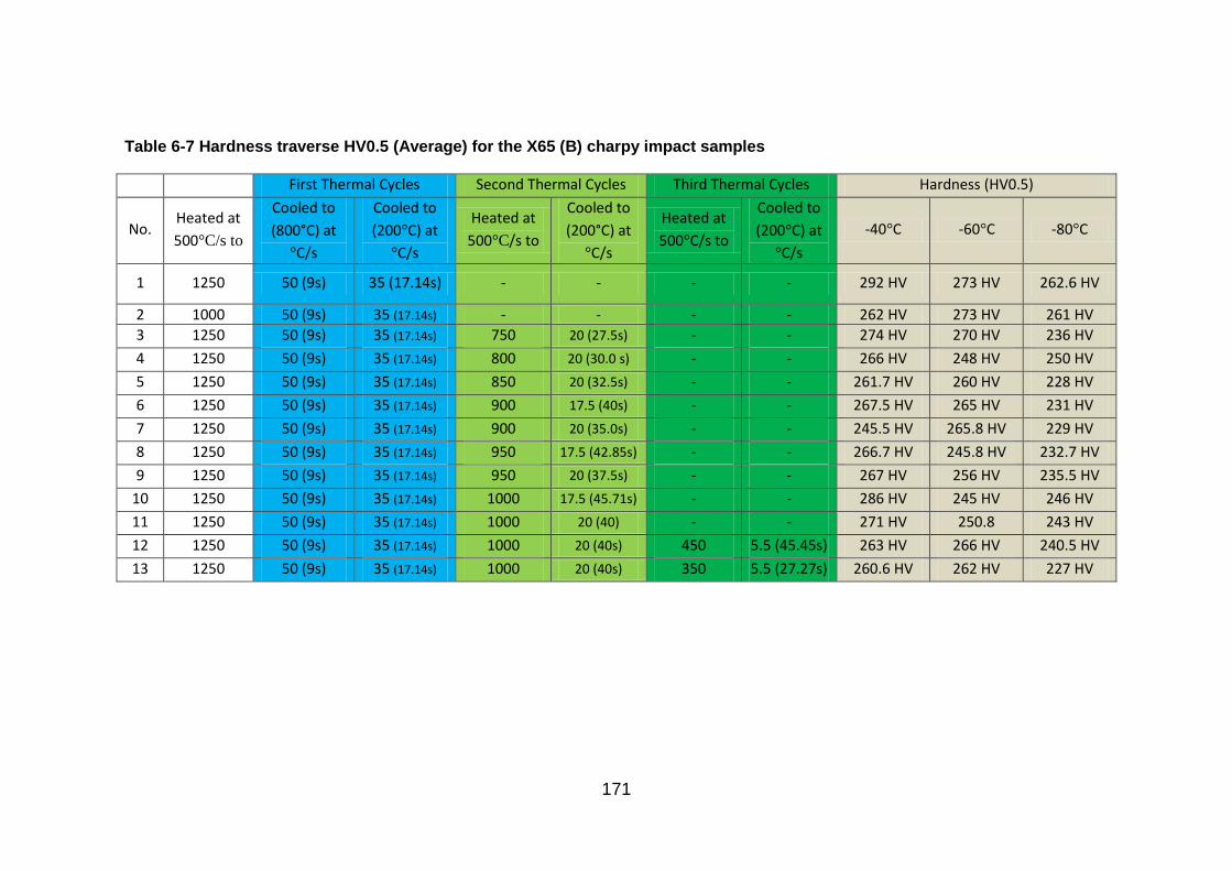
171

Table 6-7 Hardness traverse HV0.5 (Average) for the X65 (B) charpy impact samples

First Thermal Cycles Second Thermal Cycles Third Thermal Cycles Hardness (HV0.5)

No. Heated at

500°C/s to

Cooled to

(800°C) at

°C/s

Cooled to

(200°C) at

°C/s

Heated at

500°C/s to

Cooled to

(200°C) at

°C/s

Heated at

500°C/s to

Cooled to

(200°C) at

°C/s

-40°C -60°C -80°C

1 1250 50 (9s) 35 (17.14s) - - - - 292 HV 273 HV 262.6 HV

2 1000 50 (9s) 35 (17.14s) - - - - 262 HV 273 HV 261 HV

3 1250 50 (9s) 35 (17.14s) 750 20 (27.5s) - - 274 HV 270 HV 236 HV

4 1250 50 (9s) 35 (17.14s) 800 20 (30.0 s) - - 266 HV 248 HV 250 HV

5 1250 50 (9s) 35 (17.14s) 850 20 (32.5s) - - 261.7 HV 260 HV 228 HV

6 1250 50 (9s) 35 (17.14s) 900 17.5 (40s) - - 267.5 HV 265 HV 231 HV

7 1250 50 (9s) 35 (17.14s) 900 20 (35.0s) - - 245.5 HV 265.8 HV 229 HV

8 1250 50 (9s) 35 (17.14s) 950 17.5 (42.85s) - - 266.7 HV 245.8 HV 232.7 HV

9 1250 50 (9s) 35 (17.14s) 950 20 (37.5s) - - 267 HV 256 HV 235.5 HV

10 1250 50 (9s) 35 (17.14s) 1000 17.5 (45.71s) - - 286 HV 245 HV 246 HV

11 1250 50 (9s) 35 (17.14s) 1000 20 (40) - - 271 HV 250.8 243 HV

12 1250 50 (9s) 35 (17.14s) 1000 20 (40s) 450 5.5 (45.45s) 263 HV 266 HV 240.5 HV

13 1250 50 (9s) 35 (17.14s) 1000 20 (40s) 350 5.5 (27.27s) 260.6 HV 262 HV 227 HV

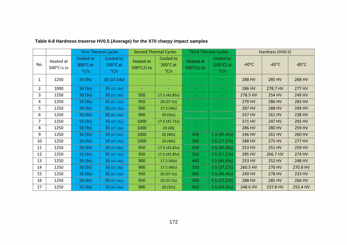
172

Table 6-8 Hardness traverse HV0.5 (Average) for the X70 charpy impact samples

First Thermal Cycles Second Thermal Cycles Third Thermal Cycles Hardness (HV0.5)

No. Heated at

500°C/s to

Cooled to

800°C at

°C/s

Cooled to

200°C at

°C/s

Heated at

500°C/s to

Cooled to

200°C at

°C/s

Heated at

500°C/s to

Cooled to

(200°C) at

°C/s

-40°C -60°C -80°C

1 1250 50 (9s) 35 (17.14s) - - - - 288 HV 285 HV 268 HV

2 1000 50 (9s) 35 (17.14s) - - - - 286 HV 278.7 HV 277 HV

3 1250 50 (9s) 35 (17.14s) 950 17.5 (42.85s) - - 278.5 HV 254 HV 249 HV

4 1250 50 (9s) 35 (17.14s) 950 20 (37.5s) - - 279 HV 286 HV 283 HV

5 1250 50 (9s) 35 (17.14s) 900 17.5 (40s) - - 287 HV 288 HV 249 HV

6 1250 50 (9s) 35 (17.14s) 900 20 (35s) - - 257 HV 261 HV 238 HV

7 1250 50 (9s) 35 (17.14s) 1000 17.5 (45.71s) - - 271 HV 247 HV 292 HV

8 1250 50 (9s) 35 (17.14s) 1000 20 (40) - - 286 HV 280 HV 259 HV

9 1250 50 (9s) 35 (17.14s) 1000 20 (40s) 450 5.5 (45.45s) 246 HV 261 HV 260 HV

10 1250 50 (9s) 35 (17.14s) 1000 20 (40s) 350 5.5 (27.27s) 288 HV 275 HV 277 HV

11 1250 50 (9s) 35 (17.14s) 950 17.5 (42.85s) 450 5.5 (45.45s) 253 HV 251 HV 259 HV

12 1250 50 (9s) 35 (17.14s) 950 17.5 (42.85s) 350 5.5 (27.27s) 285 HV 266.7 HV 274 HV

13 1250 50 (9s) 35 (17.14s) 900 17.5 (40s) 450 5.5 (45.45s) 253 HV 252 HV 248 HV

14 1250 50 (9s) 35 (17.14s) 900 17.5 (40s) 350 5.5 (27.27s) 260.5 HV 270 HV 270.8 HV

15 1250 50 (9s) 35 (17.14s) 950 20 (37.5s) 450 5.5 (45.45s) 249 HV 278 HV 233 HV

16 1250 50 (9s) 35 (17.14s) 950 20 (37.5s) 350 5.5 (27.27s) 288 HV 285 HV 266 HV

17 1250 50 (9s) 35 (17.14s) 900 20 (35s) 450 5.5 (45.45s) 248.6 HV 237.8 HV 255.4 HV

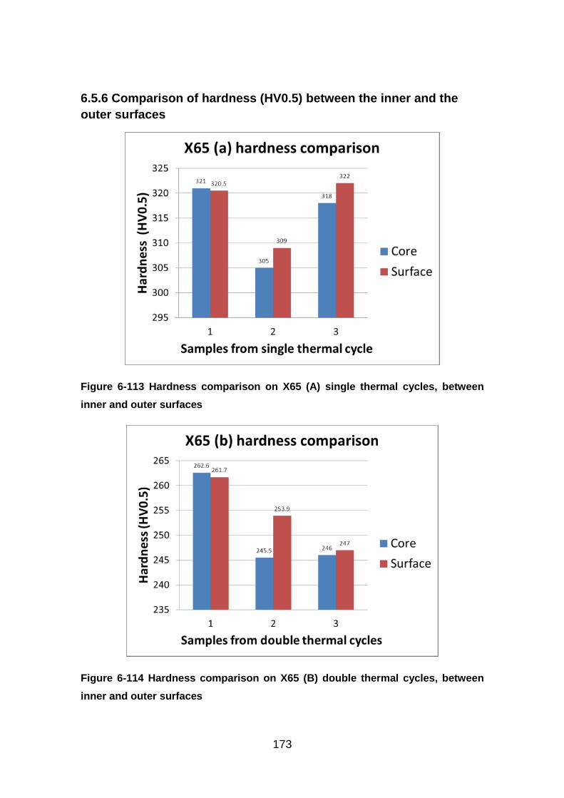
173

6.5.6 Comparison of hardness (HV0.5) between the inner and the

outer surfaces

Figure 6-113 Hardness comparison on X65 (A) single thermal cycles, between

inner and outer surfaces

Figure 6-114 Hardness comparison on X65 (B) double thermal cycles, between

inner and outer surfaces

175

7 DISCUSSION

This chapter will present a critical analysis and interpretation of the results.

Direct and indirect comparisons with previous research will be made, based on

the findings.

Parent materials 7.1

Under this heading, the parent materials will be discussed based on their

mechanical and microstructural differences.

7.1.1 Parent materials mechanical and metallurgical analyses

The four pipeline steels used in this research have been analysed both

mechanically and metallurgically. They all happen to be different from one

another in one way or the other.

The X65 (a) seamless pipes with a wall thickness of 25.4 mm in the as rolled

condition, is predominantly having polygonal ferrite (PF) and acicular ferrite (AF)

phases, with a very little pearlite.155; 156 While the thermo mechanically

processed X65 (b), with a wall thickness of 31 mm, is showing an accelerated

cooled structure, with very fine grains. Predominant phases are polygonal ferrite

(PF), acicular ferrite (AF) and some bainite (B).157

X70 pipeline steel is a TMCP material, the parent structures mainly constitute of

polygonal ferrite (PF) and bainite (B), with few acicular ferrite (AF) phases.158;

159 And the X100 grade is also a TMCP material, its main constituents are

acicular ferrite (AF) and bainite (B).159; 160

All the parent materials have satisfy the API 5L98 and DNV-OS-F101144 in terms

of microstructures, hardness, impact toughness and tensile properties as shown

in figure 6-1 to figure 6-6 on pages 79 - 85.

Hardness values (HV0.5) of the parent materials are given in figure 6-1 on page

79. X65 (a) has the lowest hardness of 191 HV0.5 and X65 (b) has 203 HV0.5.

This reflects the parent materials structures because the latter is produced

through TMCP route with a sub-micron grains structure, while the former is

176

having a rolled condition structure with larger grains. The X70 has a hardness of

209 HV0.5 and the X100 has 270 HV0.5. All the materials are within the

maximum hardness values recommended by DNV as given in table 7-1.

The yield strength (Rt0.5) and tensile strength (Rm) specified for pipeline

steels98; 144 is given in table 7-1. The average values from the samples tested

have been presented in figure 6-3 on page 80 for all the parent materials. The

maximum YS/UTS ratio has been given as 0.93 in table 7-1 for all grades.

Published data have shown that micro alloyed steels produced by accelerated

cooling generally have a lower YS/UTS ratio ranging from 0.80 to 0.90.13; 161

The X65 (a) and (b) have YS/UTS ratio of 0.81 and 0.83 respectively, while the

X70 has 0.88 and the X100 YS/UTS ratio was 0.85, as shown in figure 6-4.

Impact toughness is very important in these pipeline steels. Charpy impact

toughness (CVN) was used to characterise all the parent materials. The

average and minimum CVN for these materials at their operating temperatures

have been given in table 7-1.98; 144 The Charpy impact results for the parent

materials are shown in figure 6-2 on page 80.3; 162

As stated by the standards, the test temperatures for CVN should be the

operating temperatures, and varies from one application to another. In this

research, lower test temperatures were used throughout as worst case

scenarios, they were -40°C, -60°C and -80°C.

Table 7-1 Mechanical properties requirements for the parent materials144

Materials

Min. Yield

strength

Rt0.5

(MPa)

Min.

Tensile

Strength

Rm (MPa)

Max

Rt0.5 /

Rm

Ratio

Max. BM

Hardness

(HV10)

Average

Charpy V-

notch (J)

Min.

Charpy

V-notch

(J)

X65 450 535 0.93 270 45 38

X70 485 570 0.93 300 50 40

X100 555 625 0.93 300 56 45

177

All the four parent materials were showing an optimum CVN at -60°C, which

means that the ductile to brittle transition temperatures (DBTT) have not been

exceeded due to their excellent toughness.

Dilatometric experiments (CCT Diagrams) 7.2

Under this heading, the dilatation experiments will be explained, with respect to

dilatation curves and their interpretations. CCT diagrams will be discussed

together with the corresponding microstructures.

7.2.1 Thermal cycles and dilatation for CCTs

Total of forty seven samples from the investigated materials [12 of X65 (a), 13

of X65 (b), 11 of X70, and 11 of X100] were heated and cooled at different

cooling rates in a Gleeble 3500™ machine and a dilatometer with a resolution

of ± 2.5 mm. The samples were heated to 950°C at a distinctive heating rate of

400°C/s, this reflect the rate of heating from a real weld, as seen on the real

thermal cycles of a submerged arc weld in figure 6-60. The heating rate used in

these experiments differs from what has been reported in other papers.113; 163

Even those researchers that tried to simulate welding thermal cycles, only

heated their samples as fast as 150°C/s109 and 200°C/s164 heating rates.

The instantaneous heating normally observed in a weld is completely different

from conventional heat treatment process or slow heating. The heating rate and

the peak temperature, have a significant effect on the ferrite to austenite

transformation (α-γ), and influence the initial austenite grain size. This initial

austenite grain size condition is important in determining the final

microstructural and mechanical properties of the material.121

By using high heating rate, the material was not allowed to undergo an

equilibrium transformation. Therefore, in these experiments the samples were

taken to the austenitic region in less than 3 seconds. Depending on the initial

microstructure, there is no time for the dissolution of second phases before

crossing the AC1 and AC3 temperatures. Thereby instant transformation of areas

with higher carbon into austenite begins. Samples were then held for 300

seconds at 950°C for homogenization (austenitization).

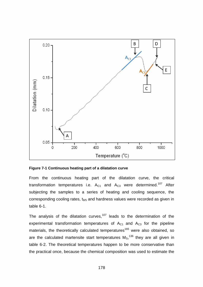
178

Figure 7-1 Continuous heating part of a dilatation curve

From the continuous heating part of the dilatation curve, the critical

transformation temperatures i.e. AC1 and AC3 were determined.107 After

subjecting the samples to a series of heating and cooling sequence, the

corresponding cooling rates, t8/5 and hardness values were recorded as given in

table 6-1.

The analysis of the dilatation curves,107 leads to the determination of the

experimental transformation temperatures of AC1 and AC3 for the pipeline

materials, the theoretically calculated temperatures165 were also obtained, so

are the calculated martensite start temperatures MS,136 they are all given in

table 6-2. The theoretical temperatures happen to be more conservative than

the practical once, because the chemical composition was used to estimate the

179

transformation temperatures using the empirical formulas. Therefore, the

available chemical analysis will influence the results, so also the present and

absent of some elements might have significant influence.136; 165

Figure 7-1 describes the continuous heating and holding part of the dilatation

curve. Points A-B represents the first part of the heating curve, at point B the

volumetric contraction due to austenite formation begins. This point is termed as

austenite transformation start (AC1). Due to increase in temperature, this

contraction compensates and reverses at point C, which is called the austenite

transformation finish (AC3). Point D represents the end of the instantaneous

heating, and corresponds to the maximum temperature. Finally, points D-E

represents the holding time of 300 seconds for austenitization.

Generally in steels, the cooling from austenitic region (γ-transformation) to room

temperature determines its final microstructure and properties. In this research,

CCT diagrams were constructed using a variety of cooling rates that covers

most of the thermal cycles in multi-pass welds. The cooling rates were selected

based on the information from the available published data.91; 109; 163; 164 The

various transformation start and finish temperatures from the austenitic

transformation were also identified.

The non-isothermal decomposition of austenite into ferrite and pearlite is shown

in figure 7-2. Points A and B were identified by extrapolating the linear portion of

the cooling part from the dilatation curve. They are considered as start and

finish points respectively. The tangential method was used to identify the

transformation points. This method makes use of tangent lines dropped on the

dilatation curve, and the point where deviation from linearity is observed, is

taken as the transformation points.107

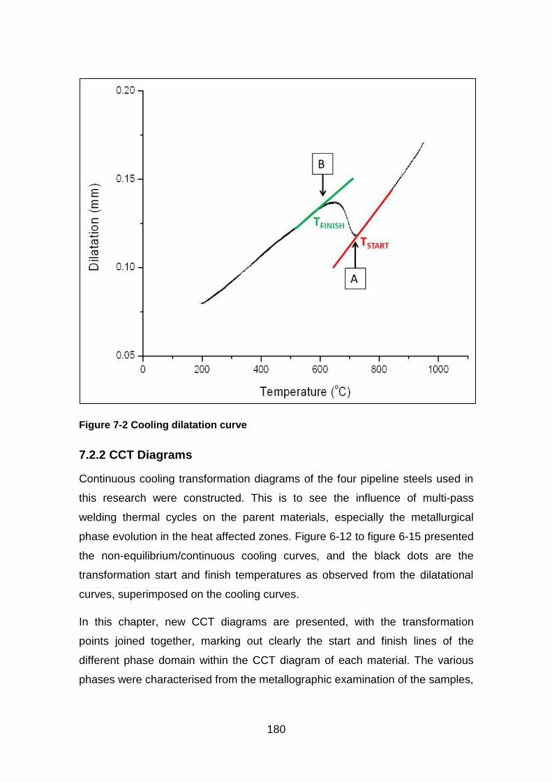
180

Figure 7-2 Cooling dilatation curve

7.2.2 CCT Diagrams

Continuous cooling transformation diagrams of the four pipeline steels used in

this research were constructed. This is to see the influence of multi-pass

welding thermal cycles on the parent materials, especially the metallurgical

phase evolution in the heat affected zones. Figure 6-12 to figure 6-15 presented

the non-equilibrium/continuous cooling curves, and the black dots are the

transformation start and finish temperatures as observed from the dilatational

curves, superimposed on the cooling curves.

In this chapter, new CCT diagrams are presented, with the transformation

points joined together, marking out clearly the start and finish lines of the

different phase domain within the CCT diagram of each material. The various

phases were characterised from the metallographic examination of the samples,

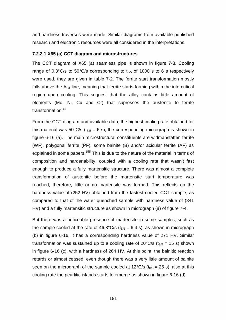
181

and hardness traverses were made. Similar diagrams from available published

research and electronic resources were all considered in the interpretations.

7.2.2.1 X65 (a) CCT diagram and microstructures

The CCT diagram of X65 (a) seamless pipe is shown in figure 7-3. Cooling

range of 0.3°C/s to 50°C/s corresponding to t8/5 of 1000 s to 6 s respectively

were used, they are given in table 7-2. The ferrite start transformation mostly

falls above the AC1 line, meaning that ferrite starts forming within the intercritical

region upon cooling. This suggest that the alloy contains little amount of

elements (Mo, Ni, Cu and Cr) that supresses the austenite to ferrite

transformation.13

From the CCT diagram and available data, the highest cooling rate obtained for

this material was 50°C/s (t8/5 = 6 s), the corresponding micrograph is shown in

figure 6-16 (a). The main microstructural constituents are widmanstätten ferrite

(WF), polygonal ferrite (PF), some bainite (B) and/or acicular ferrite (AF) as

explained in some papers.155 This is due to the nature of the material in terms of

composition and hardenability, coupled with a cooling rate that wasn’t fast

enough to produce a fully martensitic structure. There was almost a complete

transformation of austenite before the martensite start temperature was

reached, therefore, little or no martensite was formed. This reflects on the

hardness value of (252 HV) obtained from the fastest cooled CCT sample, as

compared to that of the water quenched sample with hardness value of (341

HV) and a fully martensitic structure as shown in micrograph (a) of figure 7-4.

But there was a noticeable presence of martensite in some samples, such as

the sample cooled at the rate of 46.8°C/s (t8/5 = 6.4 s), as shown in micrograph

(b) in figure 6-16, it has a corresponding hardness value of 271 HV. Similar

transformation was sustained up to a cooling rate of 20°C/s (t8/5 = 15 s) shown

in figure 6-16 (c), with a hardness of 264 HV. At this point, the bainitic reaction

retards or almost ceased, even though there was a very little amount of bainite

seen on the micrograph of the sample cooled at 12°C/s (t8/5 = 25 s), also at this

cooling rate the pearlitic islands starts to emerge as shown in figure 6-16 (d).

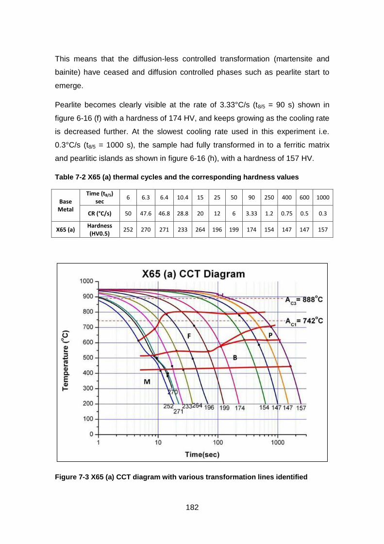
182

This means that the diffusion-less controlled transformation (martensite and

bainite) have ceased and diffusion controlled phases such as pearlite start to

emerge.

Pearlite becomes clearly visible at the rate of 3.33°C/s (t8/5 = 90 s) shown in

figure 6-16 (f) with a hardness of 174 HV, and keeps growing as the cooling rate

is decreased further. At the slowest cooling rate used in this experiment i.e.

0.3°C/s (t8/5 = 1000 s), the sample had fully transformed in to a ferritic matrix

and pearlitic islands as shown in figure 6-16 (h), with a hardness of 157 HV.

Table 7-2 X65 (a) thermal cycles and the corresponding hardness values

Base Metal

Time (t8/5) sec

6 6.3 6.4 10.4 15 25 50 90 250 400 600 1000

CR (°C/s) 50 47.6 46.8 28.8 20 12 6 3.33 1.2 0.75 0.5 0.3

X65 (a) Hardness (HV0.5)

252 270 271 233 264 196 199 174 154 147 147 157

Figure 7-3 X65 (a) CCT diagram with various transformation lines identified

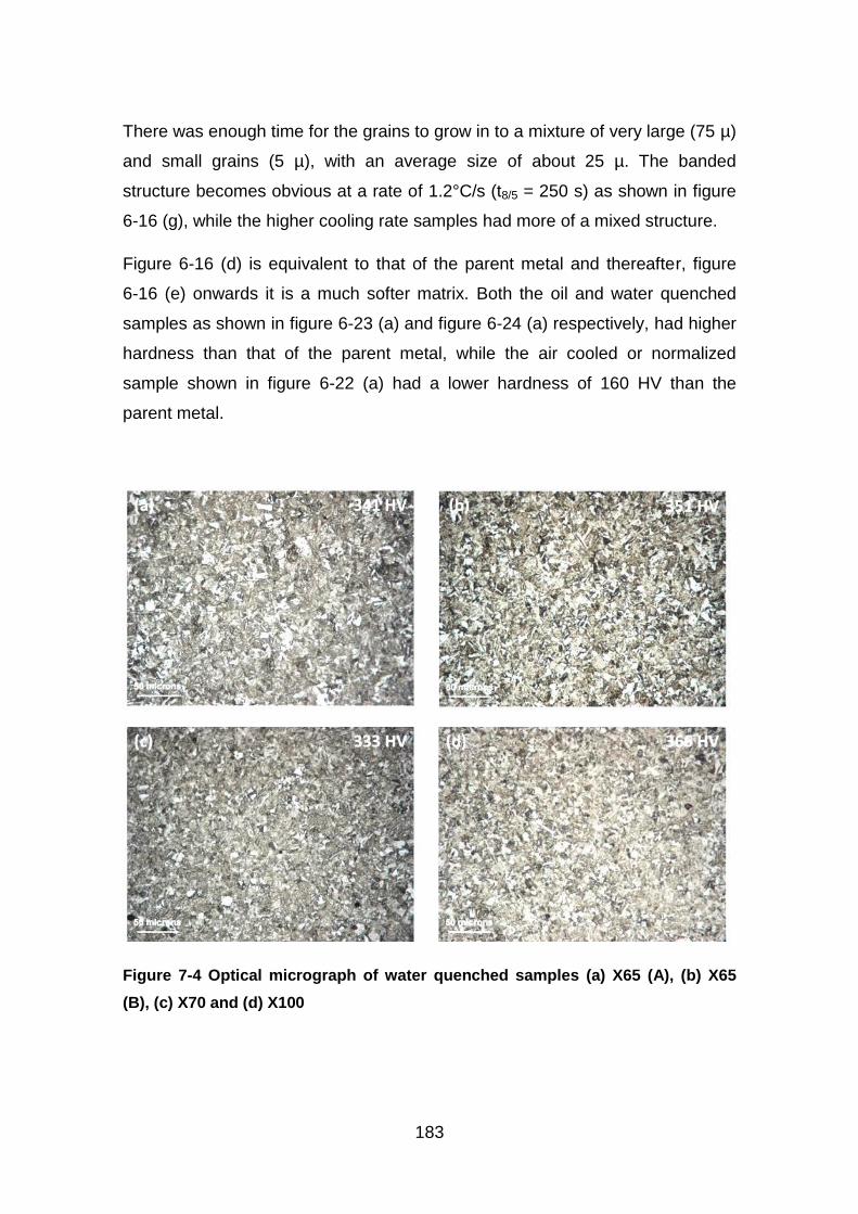
183

There was enough time for the grains to grow in to a mixture of very large (75 µ)

and small grains (5 µ), with an average size of about 25 µ. The banded

structure becomes obvious at a rate of 1.2°C/s (t8/5 = 250 s) as shown in figure

6-16 (g), while the higher cooling rate samples had more of a mixed structure.

Figure 6-16 (d) is equivalent to that of the parent metal and thereafter, figure

6-16 (e) onwards it is a much softer matrix. Both the oil and water quenched

samples as shown in figure 6-23 (a) and figure 6-24 (a) respectively, had higher

hardness than that of the parent metal, while the air cooled or normalized

sample shown in figure 6-22 (a) had a lower hardness of 160 HV than the

parent metal.

Figure 7-4 Optical micrograph of water quenched samples (a) X65 (A), (b) X65

(B), (c) X70 and (d) X100

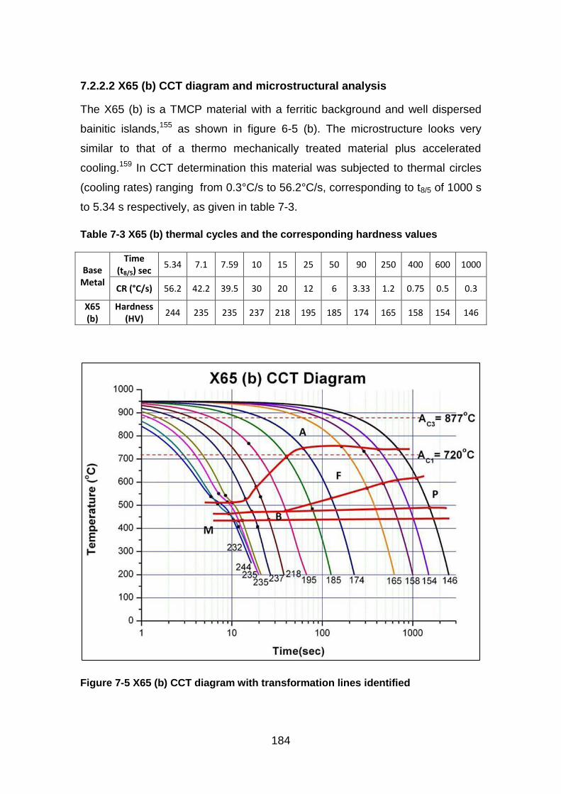
184

7.2.2.2 X65 (b) CCT diagram and microstructural analysis

The X65 (b) is a TMCP material with a ferritic background and well dispersed

bainitic islands,155 as shown in figure 6-5 (b). The microstructure looks very

similar to that of a thermo mechanically treated material plus accelerated

cooling.159 In CCT determination this material was subjected to thermal circles

(cooling rates) ranging from 0.3°C/s to 56.2°C/s, corresponding to t8/5 of 1000 s

to 5.34 s respectively, as given in table 7-3.

Table 7-3 X65 (b) thermal cycles and the corresponding hardness values

Base Metal

Time (t8/5) sec

5.34 7.1 7.59 10 15 25 50 90 250 400 600 1000

CR (°C/s) 56.2 42.2 39.5 30 20 12 6 3.33 1.2 0.75 0.5 0.3

X65 (b)

Hardness (HV)

244 235 235 237 218 195 185 174 165 158 154 146

Figure 7-5 X65 (b) CCT diagram with transformation lines identified

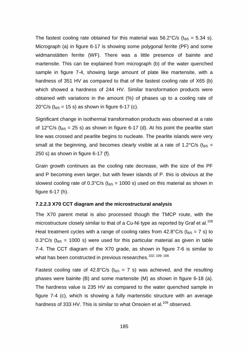
185

The fastest cooling rate obtained for this material was 56.2°C/s (t8/5 = 5.34 s).

Micrograph (a) in figure 6-17 is showing some polygonal ferrite (PF) and some

widmanstätten ferrite (WF). There was a little presence of bainite and

martensite. This can be explained from micrograph (b) of the water quenched

sample in figure 7-4, showing large amount of plate like martensite, with a

hardness of 351 HV as compared to that of the fastest cooling rate of X65 (b)

which showed a hardness of 244 HV. Similar transformation products were

obtained with variations in the amount (%) of phases up to a cooling rate of

20°C/s (t8/5 = 15 s) as shown in figure 6-17 (c).

Significant change in isothermal transformation products was observed at a rate

of 12°C/s (t8/5 = 25 s) as shown in figure 6-17 (d). At his point the pearlite start

line was crossed and pearlite begins to nucleate. The pearlite islands were very

small at the beginning, and becomes clearly visible at a rate of 1.2°C/s (t8/5 =

250 s) as shown in figure 6-17 (f).

Grain growth continues as the cooling rate decrease, with the size of the PF

and P becoming even larger, but with fewer islands of P. this is obvious at the

slowest cooling rate of 0.3°C/s (t8/5 = 1000 s) used on this material as shown in

figure 6-17 (h).

7.2.2.3 X70 CCT diagram and the microstructural analysis

The X70 parent metal is also processed though the TMCP route, with the

microstructure closely similar to that of a Cu-Ni type as reported by Graf et al.158

Heat treatment cycles with a range of cooling rates from 42.8°C/s (t8/5 = 7 s) to

0.3°C/s (t8/5 = 1000 s) were used for this particular material as given in table

7-4. The CCT diagram of the X70 grade, as shown in figure 7-6 is similar to

what has been constructed in previous researches.102; 109; 166

Fastest cooling rate of 42.8°C/s (t8/5 = 7 s) was achieved, and the resulting

phases were bainite (B) and some martensite (M) as shown in figure 6-18 (a).

The hardness value is 235 HV as compared to the water quenched sample in

figure 7-4 (c), which is showing a fully martensitic structure with an average

hardness of 333 HV. This is similar to what Onsoien et al.109 observed.

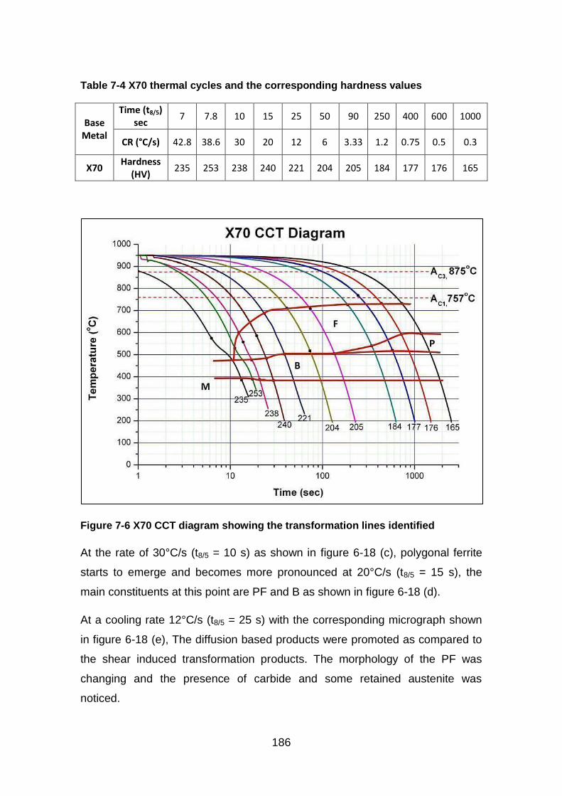
186

Table 7-4 X70 thermal cycles and the corresponding hardness values

Base Metal

Time (t8/5) sec

7 7.8 10 15 25 50 90 250 400 600 1000

CR (°C/s) 42.8 38.6 30 20 12 6 3.33 1.2 0.75 0.5 0.3

X70 Hardness

(HV) 235 253 238 240 221 204 205 184 177 176 165

Figure 7-6 X70 CCT diagram showing the transformation lines identified

At the rate of 30°C/s (t8/5 = 10 s) as shown in figure 6-18 (c), polygonal ferrite

starts to emerge and becomes more pronounced at 20°C/s (t8/5 = 15 s), the

main constituents at this point are PF and B as shown in figure 6-18 (d).

At a cooling rate 12°C/s (t8/5 = 25 s) with the corresponding micrograph shown

in figure 6-18 (e), The diffusion based products were promoted as compared to

the shear induced transformation products. The morphology of the PF was

changing and the presence of carbide and some retained austenite was

noticed.

187

Similar transformation products were observed with different morphologies up to

a rate of 3.33°C/s (t8/5 = 90 s) was reached, tiny islands of pearlite begin to

evolve as shown in figure 6-18 (f). These islands continue to grow with

decrease in cooling rate. The ferrite also changes in to large grains and keeps

growing, some grain boundary ferrite was also observed.

At the slowest cooling rate of 0.3°C/s (t8/5 = 1000 s), the sample had fully

transformed in to a well-defined structure of non-equiaxed ferrite grains of

various sizes, and pearlite colonies. This is shown in micrograph (iii) of figure

7-8, similar structures were observed by Thompson et al.167

Figure 7-7 Micrographs of the fastest cooling rates for (i) X65 (a) at t8/5 = 6 s, (ii)

X65 (b) at t8/5 = 5.34 s, (iii) X70 at t8/5 = 7 s, (iv) X100 at t8/5 = 5.34 s

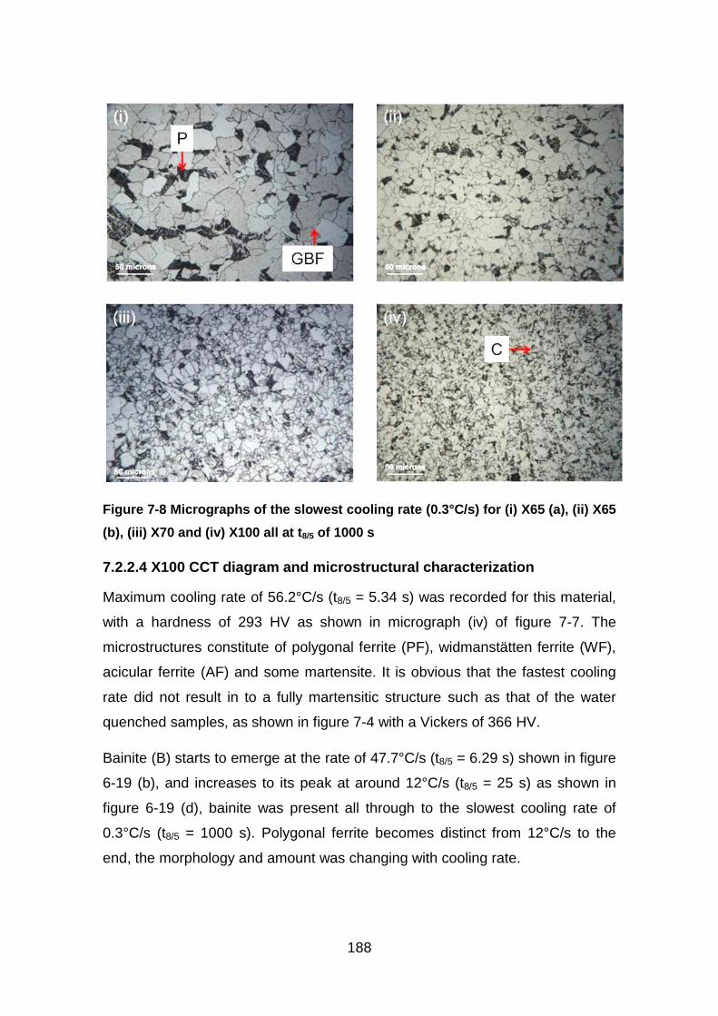
188

Figure 7-8 Micrographs of the slowest cooling rate (0.3°C/s) for (i) X65 (a), (ii) X65

(b), (iii) X70 and (iv) X100 all at t8/5 of 1000 s

7.2.2.4 X100 CCT diagram and microstructural characterization

Maximum cooling rate of 56.2°C/s (t8/5 = 5.34 s) was recorded for this material,

with a hardness of 293 HV as shown in micrograph (iv) of figure 7-7. The

microstructures constitute of polygonal ferrite (PF), widmanstätten ferrite (WF),

acicular ferrite (AF) and some martensite. It is obvious that the fastest cooling

rate did not result in to a fully martensitic structure such as that of the water

quenched samples, as shown in figure 7-4 with a Vickers of 366 HV.

Bainite (B) starts to emerge at the rate of 47.7°C/s (t8/5 = 6.29 s) shown in figure

6-19 (b), and increases to its peak at around 12°C/s (t8/5 = 25 s) as shown in

figure 6-19 (d), bainite was present all through to the slowest cooling rate of

0.3°C/s (t8/5 = 1000 s). Polygonal ferrite becomes distinct from 12°C/s to the

end, the morphology and amount was changing with cooling rate.

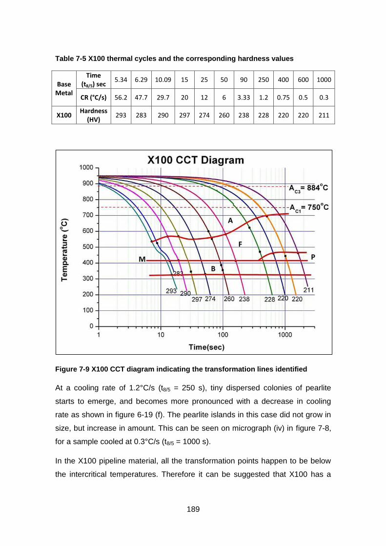
189

Table 7-5 X100 thermal cycles and the corresponding hardness values

Base Metal

Time (t8/5) sec

5.34 6.29 10.09 15 25 50 90 250 400 600 1000

CR (°C/s) 56.2 47.7 29.7 20 12 6 3.33 1.2 0.75 0.5 0.3

X100 Hardness

(HV) 293 283 290 297 274 260 238 228 220 220 211

Figure 7-9 X100 CCT diagram indicating the transformation lines identified

At a cooling rate of 1.2°C/s (t8/5 = 250 s), tiny dispersed colonies of pearlite

starts to emerge, and becomes more pronounced with a decrease in cooling

rate as shown in figure 6-19 (f). The pearlite islands in this case did not grow in

size, but increase in amount. This can be seen on micrograph (iv) in figure 7-8,

for a sample cooled at 0.3°C/s (t8/5 = 1000 s).

In the X100 pipeline material, all the transformation points happen to be below

the intercritical temperatures. Therefore it can be suggested that X100 has a

190

low temperature transformation all through.164 At a comparatively slower cooling

rate, the C-curve shifted to the right in the case of X100 grade, thereby more

diffusion-less transformation products are produced.

7.2.3 Hardness versus log t8/5 plots

Figure 6-25 presents the plot of the hardness against the cooling rate

represented by t8/5. As expected, the general trend was reduction in hardness

with decrease of the cooling rate.109; 168 The decrease was rapid from fast to

intermediate cooling rates, and becomes more steady at slower cooling rates.

This is as a result of the formation of larger amounts of ferrite, due to grain

growth and recrystallization that is increasing with decreasing cooling rates (i.e.

shift from diffusion-less to diffusion controlled transformation).113; 167; 169.

An interesting feature of the plot is the reversal in hardness distribution trends

observed at the higher cooling rates in all the steel grades used. This is similar

to what Fonda and Spanos163 and Yue et al.164 have observed. The latter

explained the hardness peaks to be where the martensitic transformation

finished, and the drop in hardness was defined as the point where bainitic

transformation replaces the martensitic transformation.

Another possible explanation is that at the higher cooling rates, where

martensitic transformation is feasible, the hardness is at its peak. When the

martensitic transformation is slow, then there will be more retained austenite

formed, while if the transformation product is entirely bainitic, then retained

austenite formation will decrease. This leads to the drop in hardness as retained

austenite is softer than bainite. As the cooling rate decreases bainitic

transformation will start, and more bainite is formed which is harder than

retained austenite, leading to the increase in hardness.

7.2.4 Comparison between the four steels

A fully martensitic structure wasn’t obtained in any of the four steel grades. This

is due to the nature of the samples size170 used, and the capability of the

thermal simulator (absence of a suitable quenching medium).109; 164 This make

the maximum cooling rate (300°C/s) that was targeted to be impossible.

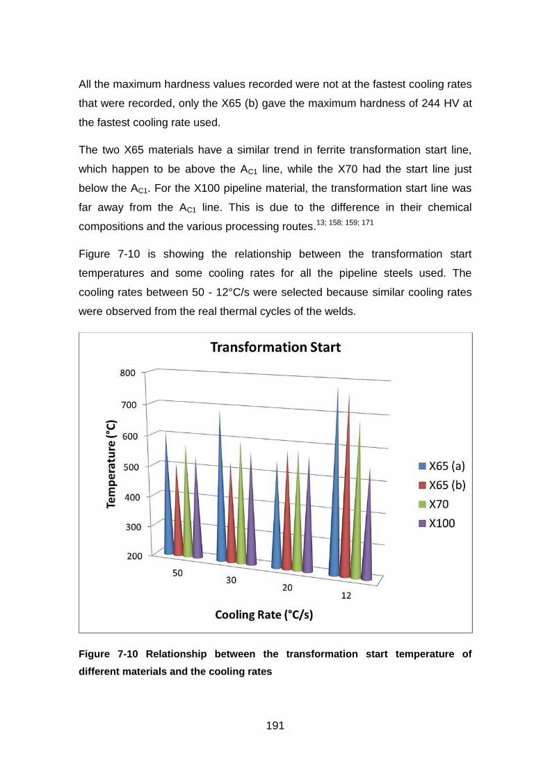
191

All the maximum hardness values recorded were not at the fastest cooling rates

that were recorded, only the X65 (b) gave the maximum hardness of 244 HV at

the fastest cooling rate used.

The two X65 materials have a similar trend in ferrite transformation start line,

which happen to be above the AC1 line, while the X70 had the start line just

below the AC1. For the X100 pipeline material, the transformation start line was

far away from the AC1 line. This is due to the difference in their chemical

compositions and the various processing routes.13; 158; 159; 171

Figure 7-10 is showing the relationship between the transformation start

temperatures and some cooling rates for all the pipeline steels used. The

cooling rates between 50 - 12°C/s were selected because similar cooling rates

were observed from the real thermal cycles of the welds.

Figure 7-10 Relationship between the transformation start temperature of

different materials and the cooling rates

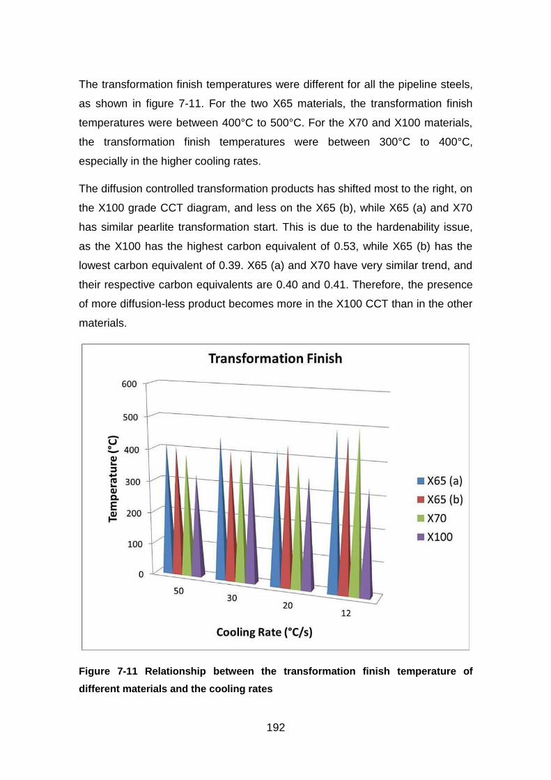
192

The transformation finish temperatures were different for all the pipeline steels,

as shown in figure 7-11. For the two X65 materials, the transformation finish

temperatures were between 400°C to 500°C. For the X70 and X100 materials,

the transformation finish temperatures were between 300°C to 400°C,

especially in the higher cooling rates.

The diffusion controlled transformation products has shifted most to the right, on

the X100 grade CCT diagram, and less on the X65 (b), while X65 (a) and X70

has similar pearlite transformation start. This is due to the hardenability issue,

as the X100 has the highest carbon equivalent of 0.53, while X65 (b) has the

lowest carbon equivalent of 0.39. X65 (a) and X70 have very similar trend, and

their respective carbon equivalents are 0.40 and 0.41. Therefore, the presence

of more diffusion-less product becomes more in the X100 CCT than in the other

materials.

Figure 7-11 Relationship between the transformation finish temperature of

different materials and the cooling rates

193

Submerged arc welding 7.3

Submerged arc welding has been known for its high productivity, high

deposition rate in excess of 27 – 45 kg/hour and high reliability.172 The

submerged arc welding experiments were carried out in two stages, i.e. the

bead on plate (BOP) welding and the full welds as was presented in chapter 6.

The discussion will be based on the welding processes and the results

obtained.

7.3.1 Bead on plate (BOP) welds

The bead on plate welds were made as trials towards the final welds, but a

significant amount of information was gathered from the data. The trials were

necessary, to see the possibility of using thermocouples to capture the true

thermal cycles of the welds. Figure 6-26 to figure 6-29 on pages 112 - 113 are

showing the macrographs of the BOP welds. It can be seen how the welds

beads interact with each other, and how the increase in penetration was caused

by the subsequent beads. Thermocouples positions are also visible on the

macrographs.

Figure 6-30 on page 116 is showing the SEM micrographs of the BOP weld

metal, at the hardness traverse positions. The micrographs were showing an

evidence of grain growth from figures (a) with a single pass toward (d) with four

passes, similar trend was observed by Keehan et al.91 The main constituents of

the weld metal are acicular ferrite (AF), polygonal ferrite (PF), bainite (B) and

some martensite (M).173 This is obvious from the hardness traverses both along

and across the welds as shown in figure 6-31 on page 117.

The hardness reduces with increase in number of passes and grain size.

Lowest hardness values were displayed by weld four as shown in figure 6-31,

which is a direct consequence of the reheating or tempering effect from the

subsequent weld beads.

The thermal cycles shown in figure 6-32 on page 118 were showing the thermal

cycle histories recorded from the same position after all the four passes have

been deposited.

194

Table 7-6 Thermal cycles data from the BOP welds

Weld and TC Numbers Max Temp (°C) t800

(sec) t500

(sec) t8/5

(sec)

Weld 1, Pass 1, TC-5 1396 16.79 30.99 14.50

Weld 2, Pass 1, TC-5 1414 22.57 37.62 15.05

Weld 3, Pass 1, TC-5 1089 8.083 22.36 14.28

Weld 4, Pass 1, TC-5 1025 9.7 25.62 15.92

The thermocouples relative positions at 10 mm and 17 mm are shown in figure

5-5 on page 61. The cooling rates represented by t8/5 are given in table 7-6.

They are not far from the range of t8/5 = 3 – 13 s suggested by Keehan et al.91

where good strength and toughness are achieved. While the reheated beads

especially in weld 4 were becoming coarser as the cooling rate decreases.

Rojko and Gliha174 reported that weld metals are generally more stable and not

affected very much by the thermal cycles of the subsequent passes, this is

because the kinetics of austenite transformation is faster in the HAZ than in the

weld metal.

7.3.2 Full submerged arc welds

The welding parameters used in these experiments were all developed and

tested at Cranfield University. They are given in the welding procedure

specifications in Appendix A.1 for all the SAW full welds made on X65 (a), X65

(b) and X70 pipeline steel grades.

There was a problem with slag removal at the beginning, which was attributed

to the welding parameters used. A high voltage of 33 V was used at the

beginning, which means reduced electrode melting rate and increased flux

consumption.175-177 Therefore, the more molten flux is in the groove, the more

difficult to remove the solidified slag, due to the nature of the groove (Narrow

groove).

The high voltage also leads to a concave deposited weld bead, which causes

the flux to get trapped and difficult to remove.

195

This problem was corrected by reducing the voltage from 33 V to 26 - 28 V and

reducing the amount of flux in the flux holder. Lower voltage results in a convex

weld bead, leading to an easy removal of the flux.26; 178

The macrographs shown in figure 6-33 to figure 6-38 on pages 119 - 121 are

the representative macrographs of the full submerged arc welds, showing the

thermocouples positions in some cases. They are all showing the interaction

and overlapping of the weld passes.

The optical micrographs of the different materials are presented in figure 6-39 to

figure 6-54 on pages 122 - 132. They are showing the microstructures at

different positions of the welds, including the heat affected zones, the fusion line

and part of the weld metal. They are indicating how the various parent materials

are responding to the welding thermal cycles, and the resulting phase

formations.

7.3.2.1 X65 (a) SAW analysis

The HAZ of the X65 (a) SAW is showing large prior austenite grains as shown

in figure 6-39 on page 122, this is the case for the HAZ at mid thickness (i.e. 15

mm from the bottom). The HAZ at 10 mm from the bottom differs from the

above, because it has been completely transformed by the internal pass. And

the structure becomes that of a bainitic phase with some widmanstätten ferrite.

The SEM micrograph of the HAZ at 10 mm is also showing the presence of

bainite as shown in figure 6-42.

Figure 6-57 on page 135, is showing the hardness traverses of the X65 (a),

which is supporting the microstructures of the HAZ at the 10 mm from the

bottom. This is because welds 1 and 2 were showing higher hardness at the

bottom than at the middle and the top. But in weld 3, the hardness at the bottom

drops, this can be related to the higher heat input recorded for the internal pass

in weld 3 (H.I. = 1.69 kJ/mm) as given in Appendix A.1. This leads to the

tempering of both the weld metal and the CGHAZ formed by the root pass,

thereby dropping the hardness lower than in the other welds.

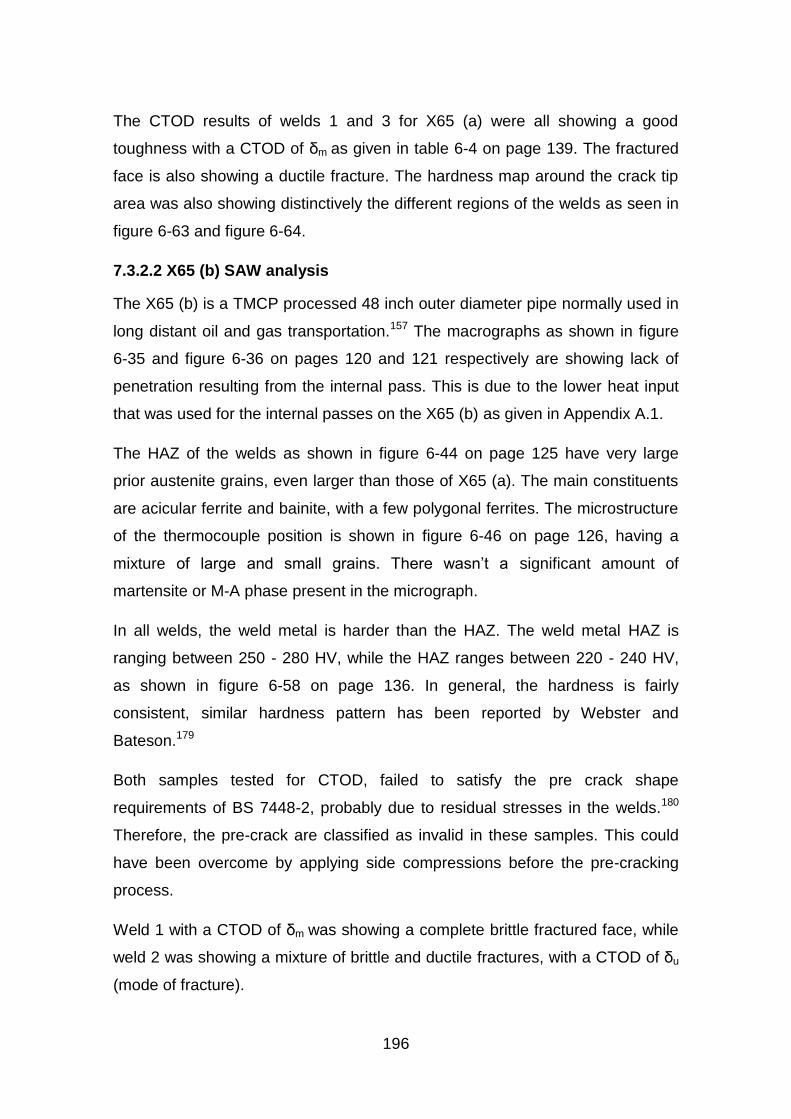
196

The CTOD results of welds 1 and 3 for X65 (a) were all showing a good

toughness with a CTOD of δm as given in table 6-4 on page 139. The fractured

face is also showing a ductile fracture. The hardness map around the crack tip

area was also showing distinctively the different regions of the welds as seen in

figure 6-63 and figure 6-64.

7.3.2.2 X65 (b) SAW analysis

The X65 (b) is a TMCP processed 48 inch outer diameter pipe normally used in

long distant oil and gas transportation.157 The macrographs as shown in figure

6-35 and figure 6-36 on pages 120 and 121 respectively are showing lack of

penetration resulting from the internal pass. This is due to the lower heat input

that was used for the internal passes on the X65 (b) as given in Appendix A.1.

The HAZ of the welds as shown in figure 6-44 on page 125 have very large

prior austenite grains, even larger than those of X65 (a). The main constituents

are acicular ferrite and bainite, with a few polygonal ferrites. The microstructure

of the thermocouple position is shown in figure 6-46 on page 126, having a

mixture of large and small grains. There wasn’t a significant amount of

martensite or M-A phase present in the micrograph.

In all welds, the weld metal is harder than the HAZ. The weld metal HAZ is

ranging between 250 - 280 HV, while the HAZ ranges between 220 - 240 HV,

as shown in figure 6-58 on page 136. In general, the hardness is fairly

consistent, similar hardness pattern has been reported by Webster and

Bateson.179

Both samples tested for CTOD, failed to satisfy the pre crack shape

requirements of BS 7448-2, probably due to residual stresses in the welds.180

Therefore, the pre-crack are classified as invalid in these samples. This could

have been overcome by applying side compressions before the pre-cracking

process.

Weld 1 with a CTOD of δm was showing a complete brittle fractured face, while

weld 2 was showing a mixture of brittle and ductile fractures, with a CTOD of δu

(mode of fracture).

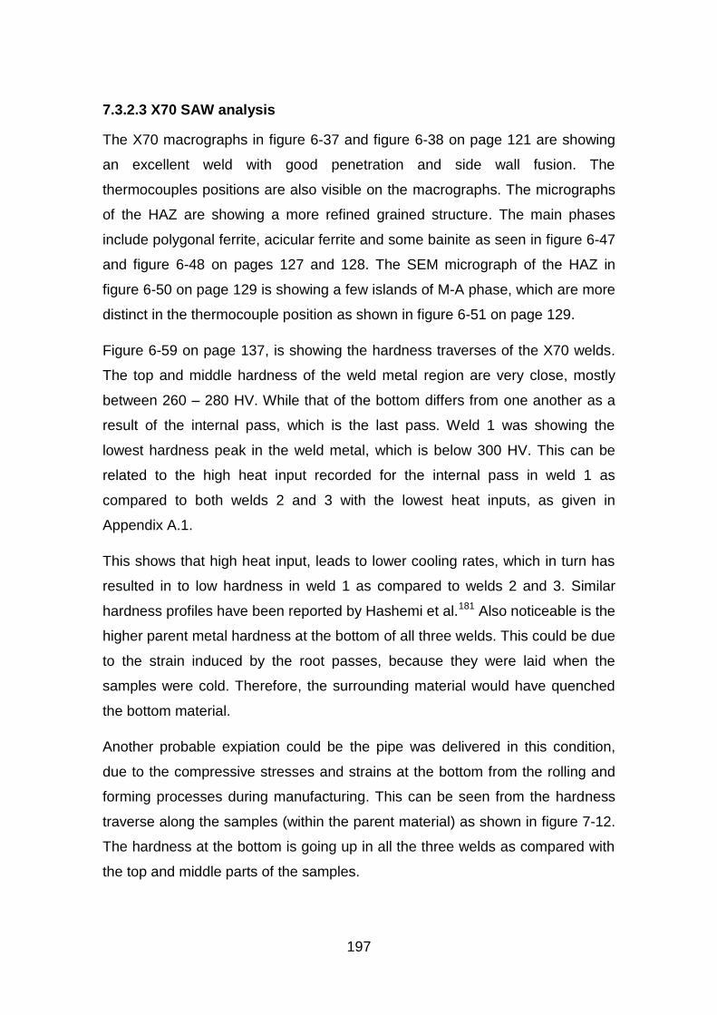
197

7.3.2.3 X70 SAW analysis

The X70 macrographs in figure 6-37 and figure 6-38 on page 121 are showing

an excellent weld with good penetration and side wall fusion. The

thermocouples positions are also visible on the macrographs. The micrographs

of the HAZ are showing a more refined grained structure. The main phases

include polygonal ferrite, acicular ferrite and some bainite as seen in figure 6-47

and figure 6-48 on pages 127 and 128. The SEM micrograph of the HAZ in

figure 6-50 on page 129 is showing a few islands of M-A phase, which are more

distinct in the thermocouple position as shown in figure 6-51 on page 129.

Figure 6-59 on page 137, is showing the hardness traverses of the X70 welds.

The top and middle hardness of the weld metal region are very close, mostly

between 260 – 280 HV. While that of the bottom differs from one another as a

result of the internal pass, which is the last pass. Weld 1 was showing the

lowest hardness peak in the weld metal, which is below 300 HV. This can be

related to the high heat input recorded for the internal pass in weld 1 as

compared to both welds 2 and 3 with the lowest heat inputs, as given in

Appendix A.1.

This shows that high heat input, leads to lower cooling rates, which in turn has

resulted in to low hardness in weld 1 as compared to welds 2 and 3. Similar

hardness profiles have been reported by Hashemi et al.181 Also noticeable is the

higher parent metal hardness at the bottom of all three welds. This could be due

to the strain induced by the root passes, because they were laid when the

samples were cold. Therefore, the surrounding material would have quenched

the bottom material.

Another probable expiation could be the pipe was delivered in this condition,

due to the compressive stresses and strains at the bottom from the rolling and

forming processes during manufacturing. This can be seen from the hardness

traverse along the samples (within the parent material) as shown in figure 7-12.

The hardness at the bottom is going up in all the three welds as compared with

the top and middle parts of the samples.

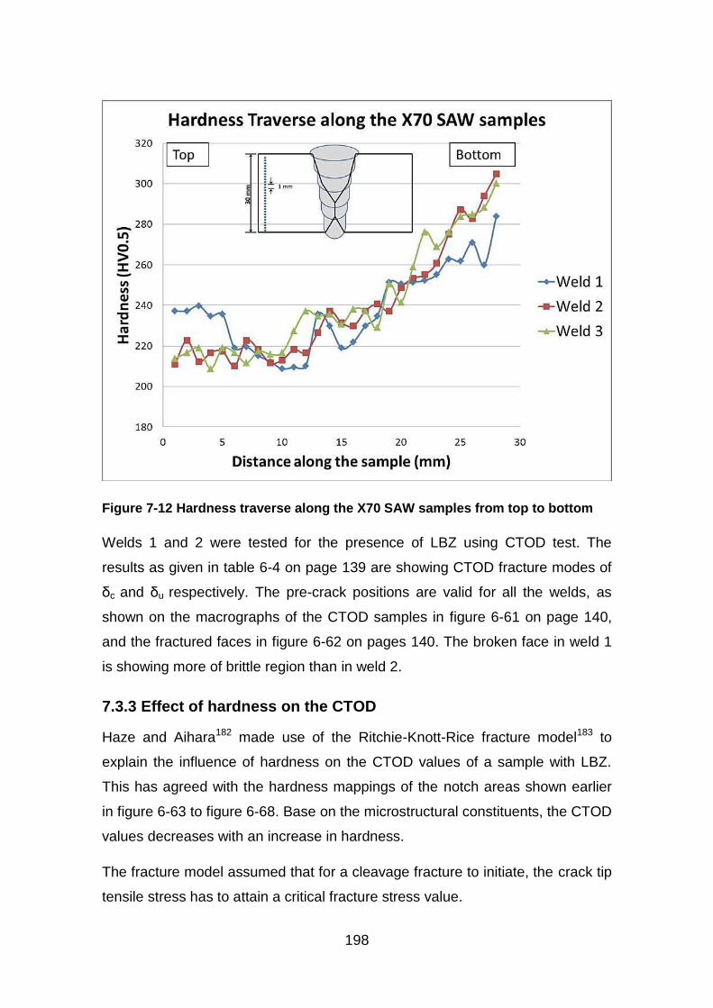
198

Figure 7-12 Hardness traverse along the X70 SAW samples from top to bottom

Welds 1 and 2 were tested for the presence of LBZ using CTOD test. The

results as given in table 6-4 on page 139 are showing CTOD fracture modes of

δc and δu respectively. The pre-crack positions are valid for all the welds, as

shown on the macrographs of the CTOD samples in figure 6-61 on page 140,

and the fractured faces in figure 6-62 on pages 140. The broken face in weld 1

is showing more of brittle region than in weld 2.

7.3.3 Effect of hardness on the CTOD

Haze and Aihara182 made use of the Ritchie-Knott-Rice fracture model183 to

explain the influence of hardness on the CTOD values of a sample with LBZ.

This has agreed with the hardness mappings of the notch areas shown earlier

in figure 6-63 to figure 6-68. Base on the microstructural constituents, the CTOD

values decreases with an increase in hardness.

The fracture model assumed that for a cleavage fracture to initiate, the crack tip

tensile stress has to attain a critical fracture stress value.

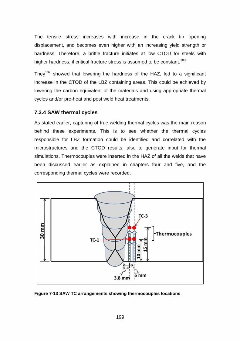
199

The tensile stress increases with increase in the crack tip opening

displacement, and becomes even higher with an increasing yield strength or

hardness. Therefore, a brittle fracture initiates at low CTOD for steels with

higher hardness, if critical fracture stress is assumed to be constant.183

They182 showed that lowering the hardness of the HAZ, led to a significant

increase in the CTOD of the LBZ containing areas. This could be achieved by

lowering the carbon equivalent of the materials and using appropriate thermal

cycles and/or pre-heat and post weld heat treatments.

7.3.4 SAW thermal cycles

As stated earlier, capturing of true welding thermal cycles was the main reason

behind these experiments. This is to see whether the thermal cycles

responsible for LBZ formation could be identified and correlated with the

microstructures and the CTOD results, also to generate input for thermal

simulations. Thermocouples were inserted in the HAZ of all the welds that have

been discussed earlier as explained in chapters four and five, and the

corresponding thermal cycles were recorded.

Figure 7-13 SAW TC arrangements showing thermocouples locations

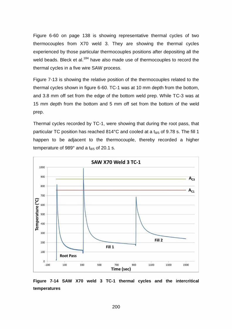
200

Figure 6-60 on page 138 is showing representative thermal cycles of two

thermocouples from X70 weld 3. They are showing the thermal cycles

experienced by those particular thermocouples positions after depositing all the

weld beads. Bleck et al.184 have also made use of thermocouples to record the

thermal cycles in a five wire SAW process.

Figure 7-13 is showing the relative position of the thermocouples related to the

thermal cycles shown in figure 6-60. TC-1 was at 10 mm depth from the bottom,

and 3.8 mm off set from the edge of the bottom weld prep. While TC-3 was at

15 mm depth from the bottom and 5 mm off set from the bottom of the weld

prep.

Thermal cycles recorded by TC-1, were showing that during the root pass, that

particular TC position has reached 814°C and cooled at a t8/5 of 9.78 s. The fill 1

happen to be adjacent to the thermocouple, thereby recorded a higher

temperature of 989° and a t8/5 of 20.1 s.

Figure 7-14 SAW X70 weld 3 TC-1 thermal cycles and the intercritical

temperatures

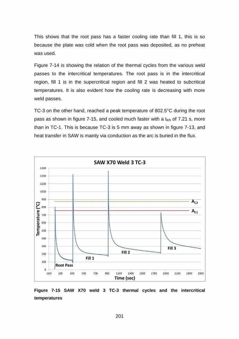
201

This shows that the root pass has a faster cooling rate than fill 1, this is so

because the plate was cold when the root pass was deposited, as no preheat

was used.

Figure 7-14 is showing the relation of the thermal cycles from the various weld

passes to the intercritical temperatures. The root pass is in the intercritical

region, fill 1 is in the supercritical region and fill 2 was heated to subcritical

temperatures. It is also evident how the cooling rate is decreasing with more

weld passes.

TC-3 on the other hand, reached a peak temperature of 802.5°C during the root

pass as shown in figure 7-15, and cooled much faster with a t8/5 of 7.21 s, more

than in TC-1. This is because TC-3 is 5 mm away as shown in figure 7-13, and

heat transfer in SAW is mainly via conduction as the arc is buried in the flux.

Figure 7-15 SAW X70 weld 3 TC-3 thermal cycles and the intercritical

temperatures

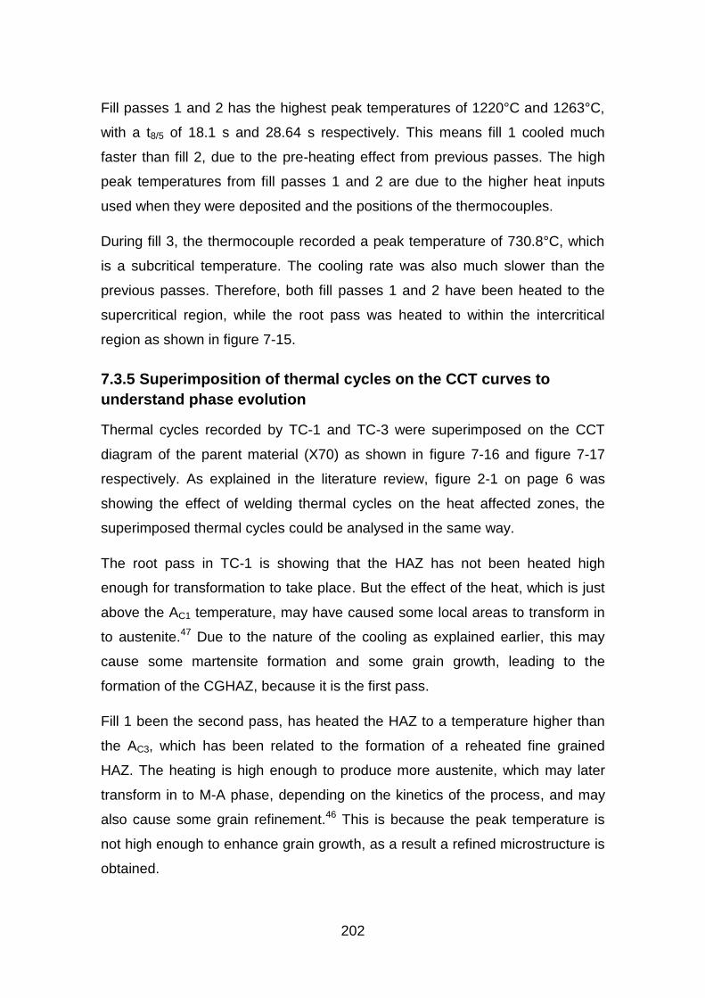
202

Fill passes 1 and 2 has the highest peak temperatures of 1220°C and 1263°C,

with a t8/5 of 18.1 s and 28.64 s respectively. This means fill 1 cooled much

faster than fill 2, due to the pre-heating effect from previous passes. The high

peak temperatures from fill passes 1 and 2 are due to the higher heat inputs

used when they were deposited and the positions of the thermocouples.

During fill 3, the thermocouple recorded a peak temperature of 730.8°C, which

is a subcritical temperature. The cooling rate was also much slower than the

previous passes. Therefore, both fill passes 1 and 2 have been heated to the

supercritical region, while the root pass was heated to within the intercritical

region as shown in figure 7-15.

7.3.5 Superimposition of thermal cycles on the CCT curves to

understand phase evolution

Thermal cycles recorded by TC-1 and TC-3 were superimposed on the CCT

diagram of the parent material (X70) as shown in figure 7-16 and figure 7-17

respectively. As explained in the literature review, figure 2-1 on page 6 was

showing the effect of welding thermal cycles on the heat affected zones, the

superimposed thermal cycles could be analysed in the same way.

The root pass in TC-1 is showing that the HAZ has not been heated high

enough for transformation to take place. But the effect of the heat, which is just

above the AC1 temperature, may have caused some local areas to transform in

to austenite.47 Due to the nature of the cooling as explained earlier, this may

cause some martensite formation and some grain growth, leading to the

formation of the CGHAZ, because it is the first pass.

Fill 1 been the second pass, has heated the HAZ to a temperature higher than

the AC3, which has been related to the formation of a reheated fine grained

HAZ. The heating is high enough to produce more austenite, which may later

transform in to M-A phase, depending on the kinetics of the process, and may

also cause some grain refinement.46 This is because the peak temperature is

not high enough to enhance grain growth, as a result a refined microstructure is

obtained.

203

Figure 7-16 Superimposition of thermal cycles of weld 3 TC-1 on the CCT of the

parent material

The effect of fill 2 from TC-1 as shown in figure 7-16 is that of a subcritically

reheated temperature, which is just below the AC1 line. Therefore, the main

structure remains, but the heating will have some annealing effect on the HAZ.46

Consequently, fill 1 would have produce a bainitic microstructure with some

polygonal ferrite as seen from the micrograph in figure 6-47 on page 127, and

fill 2 has not changed the microstructure from what it was. Thus fill 1 determines

the bulk of the final microstructure.

Looking at the superimposed thermal cycles of TC-3, as shown in figure 7-17,

the root pass being the first, has similar effects to that of TC-1. But fill passes 1

and 2 have reheated the HAZ to a very high temperature far above the AC3,

which will lead to the formation of more austenite, which means potentially more

M-A phase could be formed.

The relationship of the heat input with the peak temperatures for both TC-1 and

TC-3 are shown in figure 7-18 and figure 7-19 respectively.

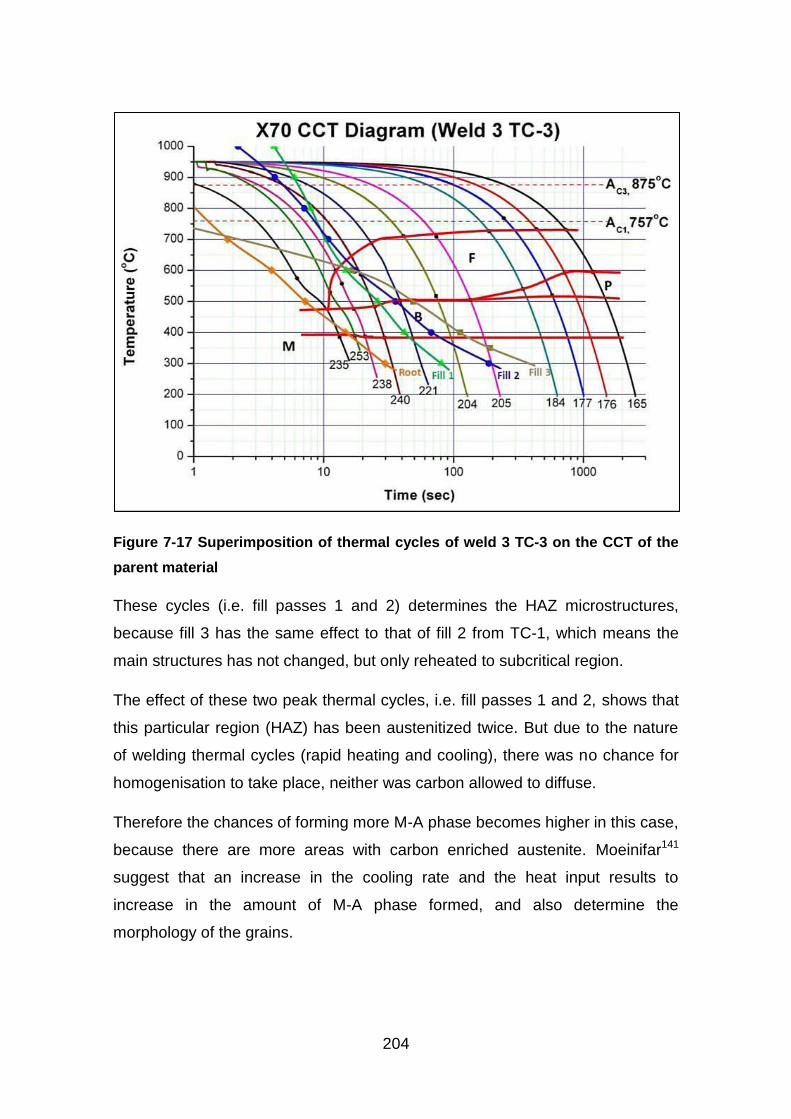
204

Figure 7-17 Superimposition of thermal cycles of weld 3 TC-3 on the CCT of the

parent material

These cycles (i.e. fill passes 1 and 2) determines the HAZ microstructures,

because fill 3 has the same effect to that of fill 2 from TC-1, which means the

main structures has not changed, but only reheated to subcritical region.

The effect of these two peak thermal cycles, i.e. fill passes 1 and 2, shows that

this particular region (HAZ) has been austenitized twice. But due to the nature

of welding thermal cycles (rapid heating and cooling), there was no chance for

homogenisation to take place, neither was carbon allowed to diffuse.

Therefore the chances of forming more M-A phase becomes higher in this case,

because there are more areas with carbon enriched austenite. Moeinifar141

suggest that an increase in the cooling rate and the heat input results to

increase in the amount of M-A phase formed, and also determine the

morphology of the grains.

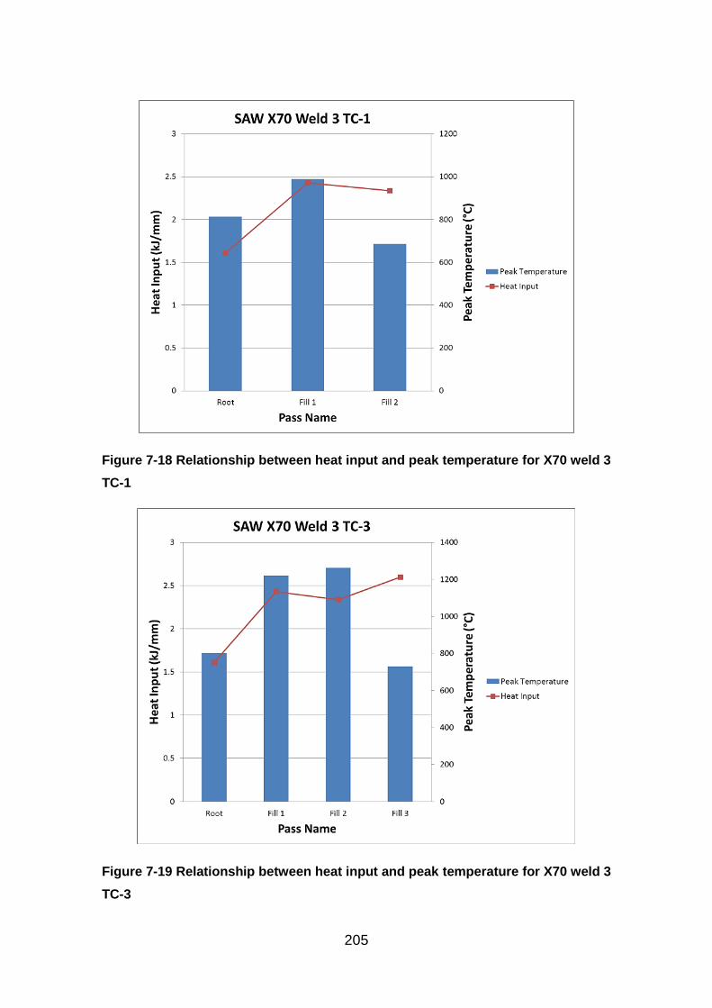
205

Figure 7-18 Relationship between heat input and peak temperature for X70 weld 3

TC-1

Figure 7-19 Relationship between heat input and peak temperature for X70 weld 3

TC-3

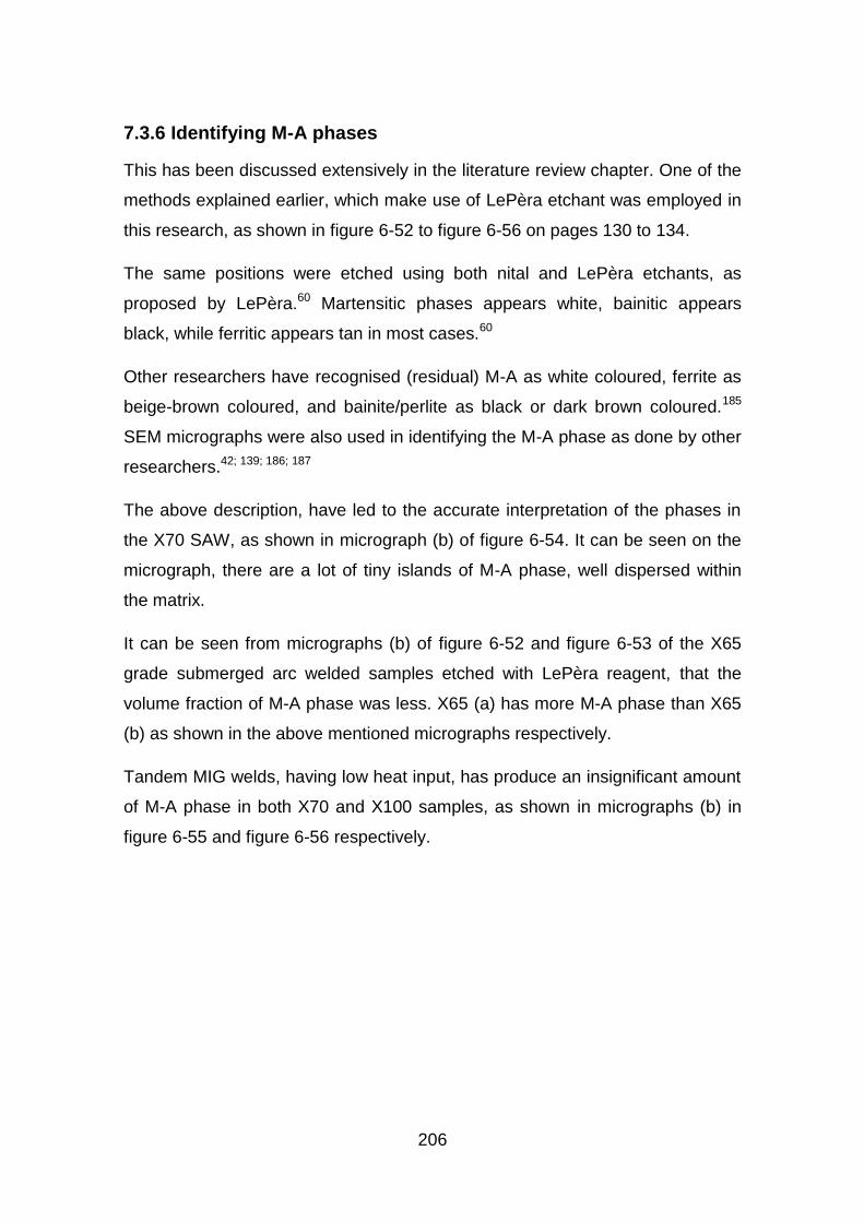
206

7.3.6 Identifying M-A phases

This has been discussed extensively in the literature review chapter. One of the

methods explained earlier, which make use of LePèra etchant was employed in

this research, as shown in figure 6-52 to figure 6-56 on pages 130 to 134.

The same positions were etched using both nital and LePèra etchants, as

proposed by LePèra.60 Martensitic phases appears white, bainitic appears

black, while ferritic appears tan in most cases.60

Other researchers have recognised (residual) M-A as white coloured, ferrite as

beige-brown coloured, and bainite/perlite as black or dark brown coloured.185

SEM micrographs were also used in identifying the M-A phase as done by other

researchers.42; 139; 186; 187

The above description, have led to the accurate interpretation of the phases in

the X70 SAW, as shown in micrograph (b) of figure 6-54. It can be seen on the

micrograph, there are a lot of tiny islands of M-A phase, well dispersed within

the matrix.

It can be seen from micrographs (b) of figure 6-52 and figure 6-53 of the X65

grade submerged arc welded samples etched with LePèra reagent, that the

volume fraction of M-A phase was less. X65 (a) has more M-A phase than X65

(b) as shown in the above mentioned micrographs respectively.

Tandem MIG welds, having low heat input, has produce an insignificant amount

of M-A phase in both X70 and X100 samples, as shown in micrographs (b) in

figure 6-55 and figure 6-56 respectively.

207

Tandem MIG welds 7.4

Narrow groove tandem MIG welding has been standardised at Cranfield

University in recent years. Previous researches145; 146; 188 have already design

acceptable welding procedure specifications using this process. In this

research, the procedure designed by Liratzis145 for X100 pipes was adopted,

and extended to the X70 pipes as modified by Girbo.189 The welding procedure

specifications given in Appendix A.2 were used for these welds.

7.4.1 Tandem MIG macrostructures

Figure 6-69 and figure 6-70 on page 144 are showing the macrographs of the

X70 narrow groove tandem MIG welds 1 and 2 respectively. The macrographs

of weld 1 are showing large porosity holes on both macrographs. While the

macrographs of weld 2 are showing some lack of side wall fusion. These could

be attributed to shielding gas and CTWD or arc length.145; 172; 190; 191

Inadequate shielding gas flow or misalignment of the gas shroud, are possible

causes of porosity. Liratzis145 proposed the use of 30 L/min gas flow rate to

overcome this problem in his work. But that was for smaller wall thickness

materials, contrary to this X70 grade which is a 31 mm thick pipe. This could be

one of the possible reasons for porosity in the weld, even though a flow rate of

30 L/min was used. Another reason might be the reaction of the weld metal with

the anti-spatter spray, which has been sprayed in the shroud and around the

weld plate.

The lack of side wall fusion might be related to the arc length and the oscillation

width. Due to the uneven nature of the jig, and the compensating characteristics

of the welders, variations in arc length are inevitable.

7.4.2 Tandem MIG microstructures

Selected optical and SEM micrographs of the tandem MIG welds are presented

in figure 6-71 to figure 6-74 from pages 145 to 147. The X70 micrograph shown

in figure 6-71 is showing from left to right the weld metal, fusion line and the

HAZ. Most of the structures are not easily resolvable at the magnifications used.

208

Some phases could be identified in the SEM macrographs shown in figure 6-74,

there are some M-A phase fraction present, and some bainitic and acicular

ferritic phases.

Figure 6-73 on page 146 is showing the X100 micrograph, also from left to right

the weld metal, the fusion line and the HAZ. The phases are more distinct in this

micrograph, as the coarse grains in the HAZ can be identified, and acicular

ferrite and polygonal ferrite are also visible.

7.4.3 Tandem MIG thermal cycles

The thermal cycles of the tandem MIG welds have been recorded using

thermocouples, as explained earlier. Capturing of the true welding thermal

cycles is the main reason behind these experiments. This is to see the effect of

the thermal cycles on the HAZ and to generate thermal cycles data to be used

in the thermal simulation experiments, as carried out with the SAW welds.

Representative thermal cycles are presented in figure 6-75 on page 148, they

are showing the recorded thermal cycles from X100 weld 1, TC-3 and TC-4.

Thermal cycles from TC-3 and TC-4 are showing peak temperatures of about

670°C and 600°C, during fill passes 3 and 4 respectively. This is based on the

thermocouples positioning used, which was shown in figure 5-14 on page 69.

These thermal cycles happen to be amongst the highest recorded throughout

the tandem MIG welds.

Therefore, it could be concluded that the thermal cycles are all within the

subcritical region, where the heat from the subsequent weld, does not change

the microstructure of the HAZ significantly, nor does it form brittle phases.

This could be related to the low heat input nature of the welding process, and

the bevel design that was used.190; 191 This led to a narrow HAZ, and a fast

cooling rate even at low temperatures, ranging between 30 - 40°C/s. Hence,

this is the reason why M-A phases are not significantly observed in these welds.

The hardness traverses also reflect the fast cooling nature of these welds, as a

maximum of about 390 HV was recorded in all the welds.

209

The HAZ was showing a bit higher hardness than the weld metal. Figure 6-76

and figure 6-77 on pages 149 and 150 are showing the hardness traverses of

the X70 and X100 pipeline steels respectively.

7.4.4 CTOD results of the X70 tandem MIG welds

The CTOD results of the X70 grade welds are given in table 6-5 on page 151.

CTOD results of weld 1 were showing a fracture mode of δm (ductile fracture),

while weld 2 have failed to satisfy the pre-crack shape requirements of BS

7448-2, which means there was a variation of more than 20% in crack length

and less than 1.3 mm minimum pre-crack length.192 This probably could have

been resolved by compressing the sides of the samples before the pre-crack.

This weld ends with a fracture mode of δc (brittle fracture).

Figure 6-78 and figure 6-79 on page 152, are showing the hardness maps of

the pre-crack region for the X70 samples. Weld 2 was showing higher hardness

values in the fusion line and HAZ, ranging between 260 – 360 HV. There are

also a few Islands with high hardness, up to about 400 HV near the fusion line.

7.4.5 Probabilistic nature of the CTOD results

Depending on the chemical composition, and processing route among others,193

M-A phases are always present in pipeline steels, even in some parent

materials, but not in large amount enough to cause brittle failure. When the

parent materials are subjected to different thermal cycles, especially in multi

pass welds the tendency to form fairly large amount of M-A phase increases.

The chance of an M-A phase causing a brittle failure in a CTOD test, generally

depends on the path taken by the crack. If the path taken happens to contain

large amount of M-A phases, or a small amount, but the M-A is fairly large in

size, then the chances of a brittle failure are very higher. But if the path taken

has little or no M-A phase, or the sizes are too small, then the chances of brittle

failure are limited.47; 194-196

210

Thermal simulations 7.5

The use of Gleeble thermo mechanical simulator to evaluate the heat affected

zones fracture toughness using charpy impact samples has become more

attractive in recent years. It offers an alternative way of generating the HAZ

microstructure uniformly through the thickness of the specimen. Even though,

thermally simulated charpy samples do not encounter problems such as

microstructural inhomogeneity and crack tip placement as compared to a weld,

they are still used as a fair representation of the HAZ.16

As presented earlier, in this research the true thermal cycles recorded from the

weld HAZ were used for these simulations, this was one of the suggestions

given by Pisarski16 in a review he wrote. Single, double and triple thermal cycles

were used to simulate the CGHAZ, ICRCGHAZ and SCRCGHAZ respectively.

Due to the nature of the thermal cycles of a weld, the heating is very fast, while

cooling is non-linear, but is changing in a step wise mode. This can be seen

from the real thermal cycles shown in figure 6-60, where cooling from the peak

temperature up to about 800°C was very fast, and then the cooling tends to

diminish from 800°C to about 200°C. Figure 5-18 on page 73 is showing the

schematic representation of the triple thermal cycles used for the gleeble

experiments.

7.5.1 Thermal cycles used for the simulation

The single thermal cycles used were divided into two groups based on peak

temperatures which are 1000°C and 1250°C, while the cooling rates remains

the same. Figure 6-80 on page 153 is a representative of the single thermal

cycles which has been heated to 1250°C. In these experiments, a cooling rate

of 50°C/s was used from the peak temperatures to 800°C, and then from 800°C

to 200°C a cooling rate of 35°C/s was used. This is in agreement with some

researchers,140; 143 though their cooling rates were not derived from real welds,

but from simulation results, such as welding software’s and finite element

analysis among others.

211

Cooling time in welding is normally defined as the time to cool from 800°C to

500°C, this is because most transformations are said to take place between this

temperature regions known as Δt8/5.14; 49 Research conducted by Ikawa et al. 52

have shown that even at temperatures below 500°C transformation does exist,

and can have a significant influence on toughness. Therefore, the need to

carefully control the temperature up to 200°C is important.52; 143

A range of peak temperatures from 750°C to 1000°C were used for the second

thermal cycles, cooling rates of 17.5°C/s and 20°C/s were also used. These

second peak temperatures were carefully selected to cover different heating

regimes within the HAZ, i.e. heating to subcritical, intercritical and supercritical

regions. The second peak temperatures used are 750°C, 800°C, 850°C, 900°C,

950°C and 1000°C, similar peak temperatures were observed from the real

welds as explained earlier. Figure 6-81 on page 154 is showing a representative

of the second thermal cycles used.

Third peak temperatures of 350°C and 450°C were used, with a constant

cooling rate of 5.5°C/s. This is because in a multi pass weld with more than two

passes, the cooling rate decreases so much due to the effect of heat

accumulation within the sample. Figure 6-82 on page 154 is a representation of

a thermal cycle with all the three peak temperatures.

7.5.2 Charpy impact results

The charpy impact samples used in the thermal simulations were tested at

different temperatures. The results were analysed based on the thermal cycles

discussed above.

7.5.2.1 Single thermal cycle

Charpy impact toughness results of the simulated single thermal cycle’s

samples are presented in figure 6-83 on page 155. The figures are showing the

results of the three materials used, i.e. X65 (a), X65 (b) and X70, as given in

Appendix B.

The results are indicating the detrimental effect of the single thermal cycles on

the impact toughness of the material grades as compared to the toughness of

212

the parent materials, as shown by the line plot in the figures mentioned. X65 (a)

is showing a significant loss of toughness when subjected to both peak

temperatures. The results are indicating decrease in toughness with decrease

in test temperature.

The X65 (b) is indicating a completely different pattern from X65 (a), at a test

temperature of -40°C, the toughness of the simulated samples was retained at

both peak temperatures. While as the test temperatures decreases, the

toughness also decreases, and it brings out the DBTT nature of the results.

On the other hand, the X70 results are not consistent like the two X65 grades.

But the samples simulated at a peak temperature of 1250°C, were all showing a

significant loss of toughness, i.e. at all test temperatures, the absorbed energy

was below 50 J. At a peak temperature of 1000°C, the absorbed charpy impact

energy at -40°C was 250 J, which happens to be more than that of the parent

material at the same temperature. At -60°C the impact energy was below 50 J

in all cases, while at -80°C the impact energy of the sample at 1000°C peak

was above 50 J.

These results are confirming the harmful effect of simulated CGHAZ on the

impact toughness of the parent materials. It can be said that both peak

temperatures are above the AC3 line and have proven to be harmful by

producing the coarse grained brittle structure. The 1250°C tend to be more

harmful, and this is because the higher the peak temperature the more

austenite that is produced. Due to the fast cooling rates associated with

welding, there is no time for diffusion, therefore the carbon enriched austenite

transforms in to a brittle phase (martensite).143

7.5.2.2 Double thermal cycles

Samples that were heated to second peak temperatures have been divided in to

two, i.e. those heated within the intercritical temperatures (below AC3), and

those heated to the supercritical temperatures (above AC3). These thermal

cycles were in addition to the single thermal cycle of 1250°C the samples have

already been subjected to.

213

The intercritically reheated samples for X65 (a) and X65 (b) have the same

cooling rates of 17.5°C/s and 20°C/s, while that of the X70 is at different cooling

rates of 10, 25 and 40°C/s. The same cooling rates were used on all the three

grades of steels for the supercritical reheating (above AC3).

Figure 6-84 on page 156, shows the charpy impact results of the intercritically

reheated X65 (a) and (b), while figure 6-85 on page 156 is for the X70. The

results are showing that the impact toughness of X65 (a) remains as bad as

those from the single thermal cycles, if not worse, while X65 (b) is showing a

different trend altogether.

The samples heated to 800°C are showing a drop in toughness at a test

temperature of -40° and -60°C, as compared to the single thermal cycles, and

they differ completely from the other intercritical temperatures. This drop of

toughness at 800°C was observed in a research conducted by Moeinifar et al.

which they related to the presence of M-A constituents.

X65 (b) samples heated to 750°C and 850°C are showing very similar trend in

the charpy impact results. At a test temperature of -40°C, the toughness was

retained in both samples, while at -60°C there was a massive gain in toughness

as compared to the single thermal cycles, while at -80° there wasn’t much

change from the energy absorbed in the single thermal cycle.

Even though, the intercritically reheated X70 samples results given in figure

6-85, cannot be compared directly with the single or triple thermal cycles due to

difference in cooling rates. The results are showing a ductile behaviour at all

test temperatures, for virtually all the samples.

The supercritically reheated samples are shown in figure 6-86 on page 157.

X65 (a) samples remain the same at all temperatures, while for the X65 (b) and

X70 there was a different trend. For the X65 (b) samples, the 950°C and

1000°C are showing a similar pattern of absorbed energy, where at a test

temperature of -40°C the samples retained their impact toughness when

compared to those from the single thermal cycles.

214

At lower test temperatures, all the samples heated to supercritical region

dropped in absorbed energy, in a similar way to the single thermal cycles. While

for a second peak of 900°C, the absorbed energy wasn’t stable like the others.

The X70 and X65 (b) samples heated to second peak temperatures of 900°C

and 1000°C were showing an opposite trend to one another. Whereas the

samples heated to a second peak of 950°C are showing a similar trend in both

material grades. The X70 is showing a loss of toughness in most cases, with

the impact toughness falling below 50 J, which is the average energy required

for an X70 material as given in table 7-1. But the 950°C samples were showing

a clearer trend, i.e. loss of toughness with decrease in test temperature.

This means that the X70 material is worse when heated to supercritical

temperatures as compared to intercritical heating. X65 (b) maintain some

degree of toughness at both intercritical and supercritical temperatures, while

X65 (a) showed a significant loss of toughness at both heating temperatures.

The increase in the intercritical temperature (second peak temperature),

generally leads to increase in the amount of transformed austenite,197 which is

rich in carbon content.52 This enriched austenite transformed into M-A phase

when subjected to favourable thermal cycles, such as those in high heat input

multi pass welding.

7.5.2.3 Triple thermal cycles

After subjecting the samples to different second peak temperatures, third peak

temperatures of 450°C and 350°C were added to samples that have been

heated to first and second peak temperatures of 1250°C and 1000°C

respectively. The results for all the material grades are given in figure 6-87 on

page 158.

Results from X65 (a) grade are showing that the third peak temperature has no

significant effect on the impact toughness. But the sample heated to a third

peak temperature of 450°C, was showing a significant increase in toughness at

a test temperature of -40°C. This could be due to the tempering effect and the

dissociation of carbides197 or an outcast.

215

The X65 (b) is showing an increase in impact toughness after been subjected to

third peak temperatures, and shows a similar trend to the X65 (a) where the

higher temperature of 450°C is showing a higher impact toughness, this is

similar to what Haze and Aihara observed.46

On the other hand, the X70 is a complete opposite of the two materials,

because the third peak temperatures did not show any improvement in the

impact toughness. The results are showing that all the samples have remained

below 50 J. This has proved the X70 to be a fully susceptible material to local

brittle zones formation. Once the LBZ formed, subsequent thermal cycles do not

recover the toughness at all, but rather only change the morphologies of the

LBZ.197

7.5.3 Effect of cooling rates used on the charpy impact results

As mentioned earlier, the thermal cycles used are identical to the real welds

thermal cycles. During the second peak thermal cycles, cooling rates of

17.5°C/s and 20°C/s were used, and figure 6-91 on page 162 is showing the

charpy impact results of the X70 material cooled at those rates.

It can be seen that the samples cooled at the two cooling rates are hard to

differentiate from each other in terms of absorbed impact energy. This is

because the cooling rates are closed to each other and therefore falls within the

same threshold, and produces quite similar results to one another. Figure 6-88

to figure 6-90 on pages 159 to 161 are agreeing to this explanation.

7.5.4 Fractography of the broken charpy impact samples

Fractographic examination of the broken charpy impact specimens for the three

materials was carried out using a scanning electron microscope at higher

magnifications. This was important in revealing the initiation sites, and to

characterise the type of crack propagation (transgranular or intergranular).21; 28;

198 and the mode of fracture, i.e. dimple, cleavage, fatigue or decohesive

rupture.199 Representative fractographs were chosen from samples fractured at

-40°C for the different heating cycles, i.e. single, double and triple thermal

cycles.

216

7.5.4.1 Single thermal cycles fractography

Fractographs of the single thermal cycles from both peak temperatures for the

X65 (a) grade are presented in figure 6-92 on page 163. The fracture mode for

both samples is of a primary cleavage, with a lot of small and uneven facets,

both are classified as brittle failures.

The X65 (b) single thermal cycles fractographs in figure 6-93 on page 163, are

showing fractograph (a) to have conical equiaxed dimples formed from micro

void coalescence, and fractograph (b) to have more of elongated dimples, both

fractures are ductile.

Contrary to the X65 grades, fractographs from the X70 single thermal cycles are

having brittle and ductile fractures, as shown in figure 6-94 on page 163.

Fractograph (a) is showing some small cleavage facets with some river lines,

while fractograph (b) is showing a mixture of large and small elongated dimples,

representing brittle and ductile fractures respectively.

7.5.4.2 Double thermal cycles fractography

From the double thermal cycles, fractographs of samples with second peak

temperatures of 1000°C, fractured at -40°C are chosen to represent these

cycles. Fractographs of X65 (a) are shown in figure 6-95 on page 164.

Fractograph (a) is showing large quasi-cleavage facets, while (b) is showing a

mixture of quasi-cleavage facets and some bands dimples, both samples are

brittle.

Figure 6-96 on page 164 is presenting the fractographs of the X65 (b) samples,

they both happen to be ductile. Fractograph (a) is showing some large facets

with river lines of a ductile nature, and some islands of elongated dimples. An

area where separation has occurred is also visible in the bottom right of the

fractograph, while fractograph (b) is mainly shear elongated dimples.

Fractographs of the X70 double thermal cycle is showing a brittle fracture in

both fractographs as shown in figure 6-97 on page 164. Fractograph (a) is

exhibiting very large quasi-cleavage facets, with some river lines, while (b) is

exhibiting more quasi-cleavage facets and some separations at the top.

217

7.5.4.3 Triple thermal cycles fractography

Triple thermal cycles were also represented by the samples fractured at -40°C,

for both peak temperatures. The fractographs of the X65 (a) are showing a

mixture of ductile and brittle fractures. Fractograph (a) is exhibiting a

combination of large elongated and conical dimples, while fractograph (b) is

more of large quasi-cleavage facets. The fractographs are shown in figure 6-98

on page 165.

X65 (b) fractographs are shown in figure 6-99 on page 165, and both happen to

be ductile. Both fractographs are exhibiting shear dimpled fracture. On the other

hand, all the fractographs of the X70 as shown in figure 6-100 on page 165 are

having a brittle fracture. Both fractographs are showing complicated fractures,

with some irregular facets.

7.5.5 Microstructural analysis of the broken charpy impact samples

The representative microstructures given in heading 6.5.4 are from the single,

double and triple thermal cycles, fractured at -40°C. These cycles represents

the various heat affected zones of a multi pass weld.

7.5.5.1 Single thermal cycles microstructures

Figure 6-101 to figure 6-103 on page 166 are the SEM micrographs of the

single thermal cycles, corresponding to the coarse grain HAZ. All the

micrographs are showing the presence of large prior austenite grains,

depending on the initial grain size, which was said to have influence in the

phases formed.200

The optical micrographs shown in figure 6-104 to figure 6-106 on page 167,

have been compared with those of the various CGHAZ from the real welds, the

similarities are obvious as seen in figure 7-20. This depends on the distance

from the fusion line and the thermal cycles used, a wide range of CGHAZ

microstructures could be characterized.140

For these experiments, all the single thermal cycles have a t8/5 of 8.57 s, this is

similar to what Li et al.143 used (i.e. t8/5 = 8 s).

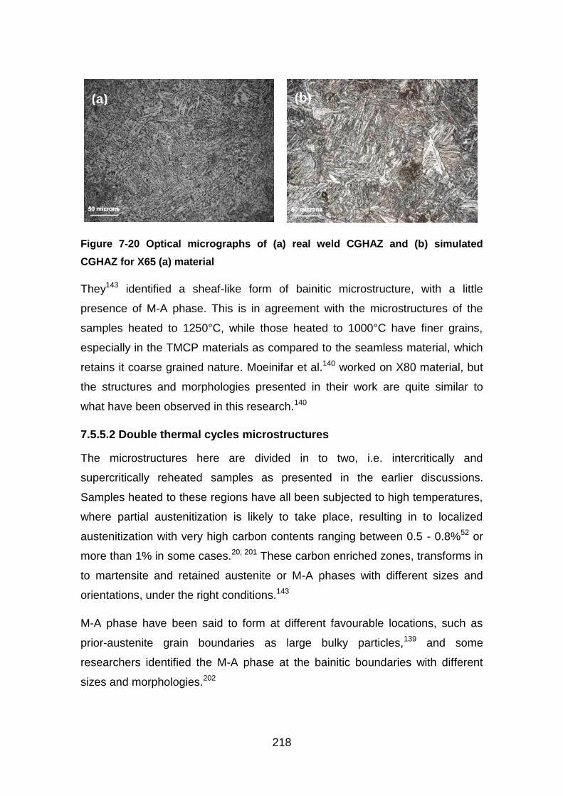
218

Figure 7-20 Optical micrographs of (a) real weld CGHAZ and (b) simulated

CGHAZ for X65 (a) material

They143 identified a sheaf-like form of bainitic microstructure, with a little

presence of M-A phase. This is in agreement with the microstructures of the

samples heated to 1250°C, while those heated to 1000°C have finer grains,

especially in the TMCP materials as compared to the seamless material, which

retains it coarse grained nature. Moeinifar et al.140 worked on X80 material, but

the structures and morphologies presented in their work are quite similar to

what have been observed in this research.140

7.5.5.2 Double thermal cycles microstructures

The microstructures here are divided in to two, i.e. intercritically and

supercritically reheated samples as presented in the earlier discussions.

Samples heated to these regions have all been subjected to high temperatures,

where partial austenitization is likely to take place, resulting in to localized

austenitization with very high carbon contents ranging between 0.5 - 0.8%52 or

more than 1% in some cases.20; 201 These carbon enriched zones, transforms in

to martensite and retained austenite or M-A phases with different sizes and

orientations, under the right conditions.143

M-A phase have been said to form at different favourable locations, such as

prior-austenite grain boundaries as large bulky particles,139 and some

researchers identified the M-A phase at the bainitic boundaries with different

sizes and morphologies.202

(a) (b)

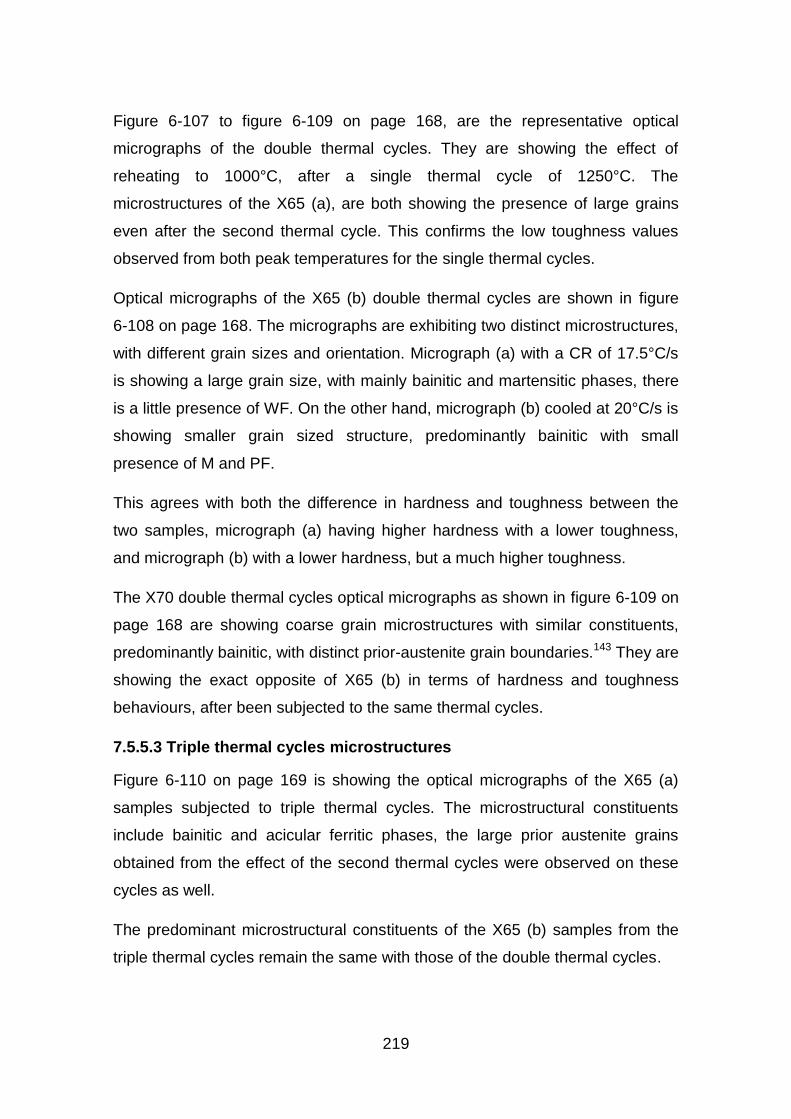
219

Figure 6-107 to figure 6-109 on page 168, are the representative optical

micrographs of the double thermal cycles. They are showing the effect of

reheating to 1000°C, after a single thermal cycle of 1250°C. The

microstructures of the X65 (a), are both showing the presence of large grains

even after the second thermal cycle. This confirms the low toughness values

observed from both peak temperatures for the single thermal cycles.

Optical micrographs of the X65 (b) double thermal cycles are shown in figure

6-108 on page 168. The micrographs are exhibiting two distinct microstructures,

with different grain sizes and orientation. Micrograph (a) with a CR of 17.5°C/s

is showing a large grain size, with mainly bainitic and martensitic phases, there

is a little presence of WF. On the other hand, micrograph (b) cooled at 20°C/s is

showing smaller grain sized structure, predominantly bainitic with small

presence of M and PF.

This agrees with both the difference in hardness and toughness between the

two samples, micrograph (a) having higher hardness with a lower toughness,

and micrograph (b) with a lower hardness, but a much higher toughness.

The X70 double thermal cycles optical micrographs as shown in figure 6-109 on

page 168 are showing coarse grain microstructures with similar constituents,

predominantly bainitic, with distinct prior-austenite grain boundaries.143 They are

showing the exact opposite of X65 (b) in terms of hardness and toughness

behaviours, after been subjected to the same thermal cycles.

7.5.5.3 Triple thermal cycles microstructures

Figure 6-110 on page 169 is showing the optical micrographs of the X65 (a)

samples subjected to triple thermal cycles. The microstructural constituents

include bainitic and acicular ferritic phases, the large prior austenite grains

obtained from the effect of the second thermal cycles were observed on these

cycles as well.

The predominant microstructural constituents of the X65 (b) samples from the

triple thermal cycles remain the same with those of the double thermal cycles.

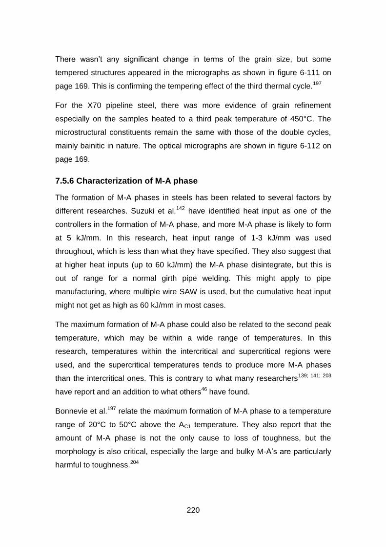
220

There wasn’t any significant change in terms of the grain size, but some

tempered structures appeared in the micrographs as shown in figure 6-111 on

page 169. This is confirming the tempering effect of the third thermal cycle.197

For the X70 pipeline steel, there was more evidence of grain refinement

especially on the samples heated to a third peak temperature of 450°C. The

microstructural constituents remain the same with those of the double cycles,

mainly bainitic in nature. The optical micrographs are shown in figure 6-112 on

page 169.

7.5.6 Characterization of M-A phase

The formation of M-A phases in steels has been related to several factors by

different researches. Suzuki et al.142 have identified heat input as one of the

controllers in the formation of M-A phase, and more M-A phase is likely to form

at 5 kJ/mm. In this research, heat input range of 1-3 kJ/mm was used

throughout, which is less than what they have specified. They also suggest that

at higher heat inputs (up to 60 kJ/mm) the M-A phase disintegrate, but this is

out of range for a normal girth pipe welding. This might apply to pipe

manufacturing, where multiple wire SAW is used, but the cumulative heat input

might not get as high as 60 kJ/mm in most cases.

The maximum formation of M-A phase could also be related to the second peak

temperature, which may be within a wide range of temperatures. In this

research, temperatures within the intercritical and supercritical regions were

used, and the supercritical temperatures tends to produce more M-A phases

than the intercritical ones. This is contrary to what many researchers139; 141; 203

have report and an addition to what others46 have found.

Bonnevie et al.197 relate the maximum formation of M-A phase to a temperature

range of 20°C to 50°C above the AC1 temperature. They also report that the

amount of M-A phase is not the only cause to loss of toughness, but the

morphology is also critical, especially the large and bulky M-A’s are particularly

harmful to toughness.204

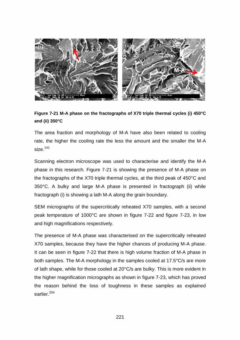
221

Figure 7-21 M-A phase on the fractographs of X70 triple thermal cycles (i) 450°C

and (ii) 350°C

The area fraction and morphology of M-A have also been related to cooling

rate, the higher the cooling rate the less the amount and the smaller the M-A

size.141

Scanning electron microscope was used to characterise and identify the M-A

phase in this research. Figure 7-21 is showing the presence of M-A phase on

the fractographs of the X70 triple thermal cycles, at the third peak of 450°C and

350°C. A bulky and large M-A phase is presented in fractograph (ii) while

fractograph (i) is showing a lath M-A along the grain boundary.

SEM micrographs of the supercritically reheated X70 samples, with a second

peak temperature of 1000°C are shown in figure 7-22 and figure 7-23, in low

and high magnifications respectively.

The presence of M-A phase was characterised on the supercritically reheated

X70 samples, because they have the higher chances of producing M-A phase.

It can be seen in figure 7-22 that there is high volume fraction of M-A phase in

both samples. The M-A morphology in the samples cooled at 17.5°C/s are more

of lath shape, while for those cooled at 20°C/s are bulky. This is more evident in

the higher magnification micrographs as shown in figure 7-23, which has proved

the reason behind the loss of toughness in these samples as explained

earlier.204

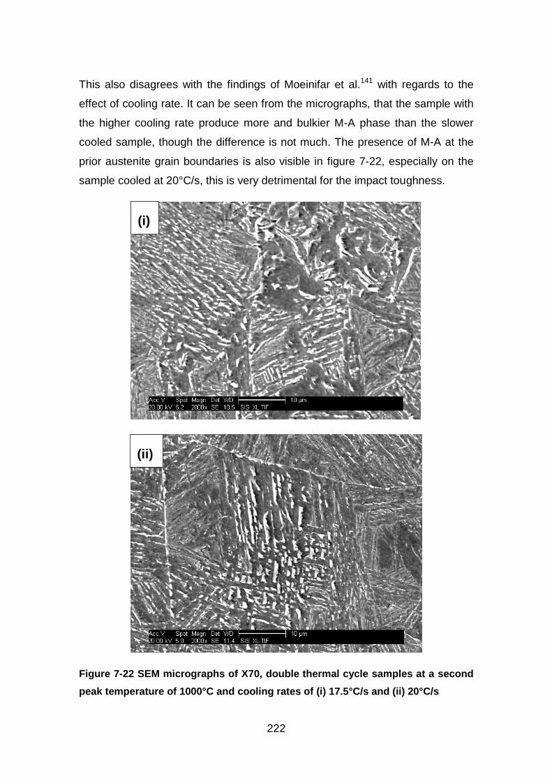
222

This also disagrees with the findings of Moeinifar et al.141 with regards to the

effect of cooling rate. It can be seen from the micrographs, that the sample with

the higher cooling rate produce more and bulkier M-A phase than the slower

cooled sample, though the difference is not much. The presence of M-A at the

prior austenite grain boundaries is also visible in figure 7-22, especially on the

sample cooled at 20°C/s, this is very detrimental for the impact toughness.

Figure 7-22 SEM micrographs of X70, double thermal cycle samples at a second

peak temperature of 1000°C and cooling rates of (i) 17.5°C/s and (ii) 20°C/s

(i)

(ii)

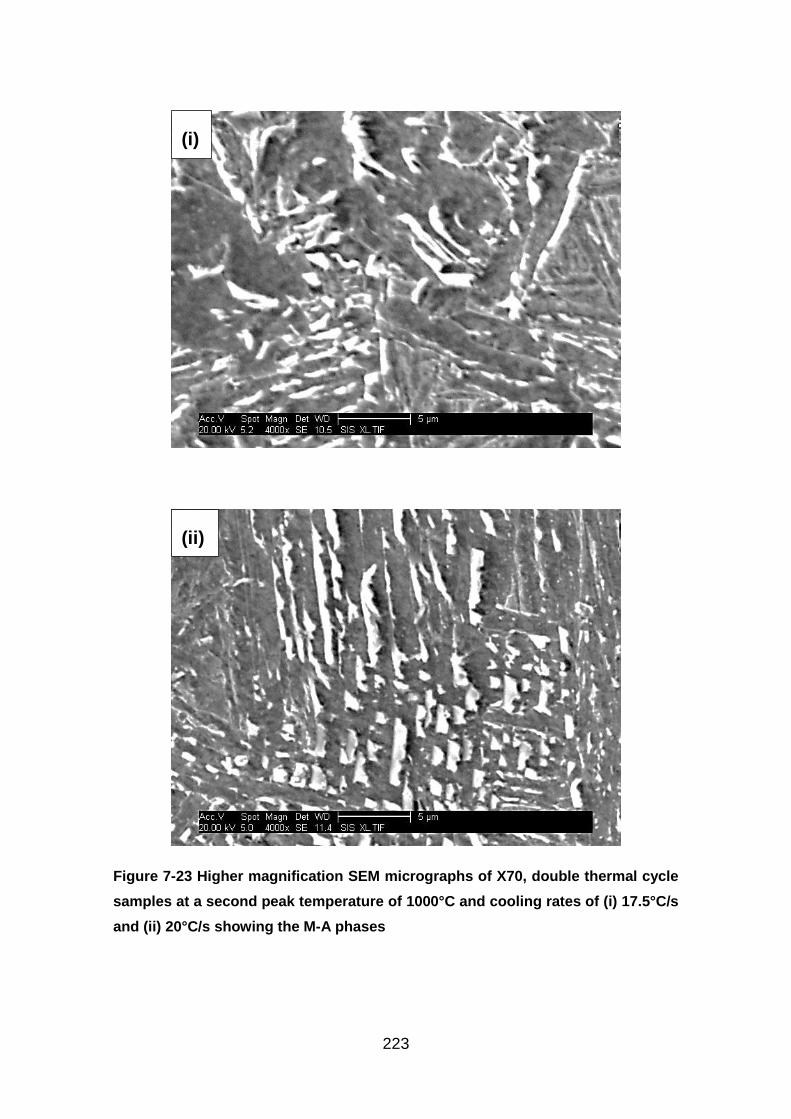
223

Figure 7-23 Higher magnification SEM micrographs of X70, double thermal cycle

samples at a second peak temperature of 1000°C and cooling rates of (i) 17.5°C/s

and (ii) 20°C/s showing the M-A phases

(ii)

(i)

224

7.5.7 Hardness traverses

The microhardness traverse results of all the materials at different thermal

cycles are given in table 6-6 to table 6-8 on pages 170 to 172. The results are

not showing any distinct relation between the microhardness values and the

charpy impact values at different test temperatures, though hardness can be

related to microstructural constituent, which have a significant influence on the

toughness of the material.182

The influence of the reheating temperatures on the microhardness of the double

thermal cycles cooled at 20°C/s, and fractured at -40°C is shown in figure 7-24.

It can be seen that there is a steady increase in hardness as the second peak

temperature is increased in the supercritical region.

This is contrary to what Moeinifar et al.139 have found that the supercritical

region is showing the lowest hardness due to grain refinement and less blocky

M-A constituents. This could be due to the difference in the cooling rates they

used, which are far from those recorded from the real welds. The trend

observed here could be due to the increase in the presence of M-A phase as

the second peak temperatures are increased.

7.5.8 Comparison of hardness between inner and outer surfaces

A random comparison between the inner and the outer surfaces of the single

thermal cycles of X65 (a) and double thermal cycles of X65 (b) was carried out.

This is to see if there is any significant difference in hardness between the case

and the core, so as to validate the uniformity of heating and cooling associated

with the Gleeble thermo mechanical simulator, as claimed by the

manufacturers.147

Figure 6-113 on page 173, is showing the hardness comparison between the

surface and the core of the single thermal cycles of the X65 (a) grade. This is a

validation process, therefore, the samples are selected randomly not in any

particular order.

225

It can be seen from the figure that the maximum difference in hardness between

the surface and the core is 4 HV, while the minimum is 0.5 HV. There isn’t a

particular trend, because in sample 1 the core is harder, while in samples 2 and

3 the surface is harder.

In the double thermal cycles, there is not much difference as well, the maximum

difference of 8.4 HV was recorded in sample 2, as shown in figure 6-114 on

page 173. The minimum difference recorded was on sample 1, with a difference

of 0.9 HV. This has confirmed the assumption that there is a fairly uniform

heating and cooling even with a 10 mm square and diameter samples.

Figure 7-24 Influence of second peak temperature on the hardness values of X65

(a), X65 (b) and X70 grades

227

8 CONCLUSIONS

From the CCT diagrams of the four API-5L steel grades, it could be

interpreted that similar thermal cycles can produce different metallurgical

phases depending on the composition, processing route and the starting

microstructures of the material.

The real welding thermal cycles recorded were showing that the HAZ,

depending on the welding process and pass sequence, have been

reheated through various temperature regions viz. subcritical, inter-

critical and supercritical part of the phase diagram.

The thermal cycles responsible for low toughness in some of the pipeline

steels have been interpreted from the real welding thermal cycles and

the results from the thermal simulation experiments. It was found that the

first and second thermal cycles are responsible for the formation of low

toughness phases in the welds. This corresponds to single and double

thermal cycles in the thermal simulations experiments.

In our given scope of investigation, the third thermal cycles have little or

no effect in most cases, but have some tempering effect on the

microstructures.

The impact toughness values of the thermal simulated samples could be

correlated to the peak temperature of the second thermal cycle for some

grades. The initial microstructure of the steel is an important factor

towards determining the influence of thermal cycles on the toughness of

the thermally simulated specimens.

The X65 (b) grade has shown significantly high toughness at both

intercritical and supercritical temperatures as compared to the other

grades. This could be due to its starting microstructure been very fine

(sub-micron size) and many other factors including chemical composition

and thermal cycles.

There is no difference in hardness between the surface and the core of

the samples when thermally simulated in the Gleeble thermo-mechanical

228

simulator. This indicates a relatively uniform heating and cooling cycles

throughout the cross section of the samples.

The formation of M-A phase is more pronounced at temperatures above

the AC3 line, i.e. supercritical temperatures. However, some samples

showed brittle behaviour even when heated to a temperature below AC1.

This can be due to several other factors which generate brittle behaviour

e.g. presence of stress raiser in the microstructure. An inhomogeneity in

composition could also be a reason for such unpredictable failures.

The amount and morphology of the M-A phase is significantly influenced

by heating in to the intercritical and supercritical regions. Other factors

that affect it include the peak temperatures and the cooling rate.

From the instrumented welds, it could be deduced that submerged arc

welding is more susceptible to the formation of M-A phase as compared

to tandem MIG welding with low heat input.

From the materials used in this research, it could be concluded that X70

grade welded with SAW is more susceptible to M-A formation than all the

other grades welded with SAW.

The materials welded with tandem MIG welding both have less chances

of M-A formation, thus better toughness properties.

This research has shown that thermal simulation can be used to evaluate

the thermal response of a material in a multiple thermal cycle situation,

and the corresponding microstructures. This can be achieved via:

Construction a CCT diagram

Thermal simulation using Charpy impact samples and thermal

cycles from a real weld

Metallurgically and mechanically analysing the samples in order to

evaluate their response to the thermal cycles

229

9 RECOMMENDATIONS

This chapter is divided into two, recommendation to companies on how they

can reduce the formation of brittle phases in multi-pass welds or to avoid them

completely where necessary. And recommendation for future work on what

should be done to continue with the research.

Recommendation to companies 9.1

The use of CCT diagrams and thermal simulation using real welding

thermal cycles to establish the susceptibility of a material to local brittle

zones formation will prove vital to pipeline steel manufacturers and

pipeline welding companies.

Multiple thermal cycles simulation is necessary to evaluate their effect on

a material, this could be achieved by using thermo mechanical

simulators.

The multiple thermal cycles for simulation should be based on the

intended heat input that will be used for a particular project.

A welding procedure specification should be designed based on the

susceptibility of the materials to LBZ. Low heat input should be used for

susceptible materials to avoid higher peak temperatures in the second

thermal cycles, which might lead to LBZ formation. While for materials

that are not susceptible, there is no harm in using the optimal heat input,

even if it is high.

Collaboration between the welding companies and the steel

manufactures in evaluating the susceptibility of the pipe material to LBZ

before embarking on a project will be very helpful.

230

Recommendation for future work 9.2

More welds should be done to explore different weld preparation and

their influence on HAZ thermal cycles.

A standardised way of attaching thermocouples should be developed

and modelled to prove it. This will ensure other researches and

companies can use the method to record thermal cycles from the HAZ of

their welds, especially in the high heat input processes.

More CTOD tests need to be carried out to accurately validate the

presence of LBZ in the welds and the simulated samples.

Modelling of the various welding processes normally used in pipeline

industries is necessary. In order to have a comprehensive understanding

of the various isotherms from different welding processes and their

consequential thermal cycles.

Computer simulation and modelling of the thermal cycles, in relation to

heat input and the resulting metallurgical phases should be carried out.

This can be validated with the available data from this research, and will

ease the processes of characterizing materials as susceptible or not

based on the given parameters.

A dilatometer should be used on the charpy impact samples used for the

HAZ simulation. This will give the transformation temperatures as well as

the respective thermal cycles. It will make it easier to locate the

transformation points on a CCT diagram for further analysis.

EBSD analysis needs to be carried out on the samples to characterize

the grains, the boundary angles, and to map the phases correctly.

Misorientation maps should be made using EBSD to accurately

characterise the presence of some phases in both the welds and in the

specimens used for simulations.

231

REFERENCES

1. Sandrea, R. and Sandrea, I. (2010), "Deep water crude oil output: How large will the uptick be?", Oil and Gas journal, vol. 108, no. 41, pp. 1-10.

2. Yapp, D. and Blackman, S. A. (2004), "Recent developments in high productivity pipeline welding", Journal of the Brazilian Society of Mechanical Sciences and Engineering, vol. 26, no. 1, pp. 89-97.

3. Liessem, A., Schröder, J., Pant, M., Erdelen-Peppler, M., Liedtke, M., Höhler, S. and Stallybrass, C. (2008), "Manufacturing challenges of high strength line pipes", New Developments on Metallurgy and Applications of High Strength Steels, Buenos Aires 2008 - Proceedings of the International Conference on New Developments on Metallurgy and Applications of High Strength steel, Vol. 1, Buenos Aires, pp. 543.

4. Demofonti, G. and Mannucci, G. (2008), "A critical review of the developed and available know how devoted to a safe use of X100 grade steel in large diameter pipelines", New Developments on Metallurgy and Applications of High Strength Steels, Buenos Aires 2008 - Proceedings of the International Conference on New Developments on Metallurgy and Applications of High Strength steels, Vol. 1, Buenos Aires, pp. 625.

5. Chunming, W., Xingfang, W., Jie, L. and Ning'an, X. (2006), "Transmission electron microscopy of martensite-austenite islands in pipeline steel X70", Materials Science and Engineering A, vol. 438, no. 440, pp. 267-271.

6. Bae, J. H., Yoo, J. Y., Kim, K., Kim, C. M. and Kang, K. B. (2006), "Development of high strength linepipe steels with excellent weldability", in Xi'an, Shaanxi 710065, China; Tubular Goods Research Centre of China National Petroleum Corp. (CNPC), .

7. Traizet, A. -., Galand, E., Chovet, C. and Leduey, B. (2008), "Welding consumables development for high strength steel joints for oil & gas applications", New Developments on Metallurgy and Applications of High Strength Steels, Buenos Aires 2008 - Proceedings of the International Conference on New Developments on Metallurgy and Applications of High Strength steels, Vol. 1, Buenos Aires, pp. 685.

8. Widgery, D. (2008), "Welding arctic pipelines", Welding in the World, vol. 52, no. SPEC. ISS., pp. 591-596.

9. U.S. Energy Information Administration (2010), Annual energy outlook 2010, DOE/EIA-0383(2010), www.eia.doe.gov/oiaf/aeo, USA.

10. Timokhina, I. B., Hodgson, P. D., Ringer, S. P., Zheng, R. K. and Pereloma, E. V. (2007), "Precipitate characterisation of an advanced high-

232

strength low-alloy (HSLA) steel using atom probe tomography", Scripta Materialia, vol. 56, no. 7, pp. 601-604.

11. Mishra, S. K., Das, S. and Ranganathan, S. (2002), "Precipitation in high strength low alloy (HSLA) steel: A TEM study", Materials Science and Engineering A, vol. 323, no. 1-2, pp. 285-292.

12. Bhadeshia, H. K. D. H. and Honeycombe, R. (2006), Steels Microstructure and Properties, 3rd ed, Elsevier, UK.

13. Sampath, K. (2006), "An understanding of HSLA-65 plate steels", Journal of Materials Engineering and Performance, vol. 15, no. 1, pp. 32-40.

14. Kou, S. (2003), Welding Metallurgy, 2nd ed, John Wiley and sons, USA.

15. Amano, K., Kudo, J., Itakura, N. and Nakano, Y. (1989), "Metallurgical and welding factors controlling local brittle zone in weld HAZ", Proceedings of the International Offshore Mechanics and Arctic Engineering Symposium, Vol. 3, pp. 683.

16. Pisarski. (TWI UK), (1996), A Review of HAZ Toughness Evaluation (unpublished Report), UK.

17. Ouro, C. R., de S. Bott, I. and Bastian, F. L. (1996), "Influence of local brittle zone size on the heat affected zone toughness of structural steel for offshore applications", ASM International (USA), pp. 519-524, 1996; ASM International (USA), pp. 519-524, 1996, 519-524, 1996;, pp. ASM International (USA), p.

18. Tian, Z. (1998), "Study on local brittle zone fracture toughness of TMCP steels", Journal of Iron and Steel Research International, vol. 10, no. 4, pp. 50-53.

19. Kenney, K. L., Reuter, W. G., Reemsnyder, H. S. and Matlock, D. K. (1997), "Fracture initiation by local brittle zones in weldments of quenched and tempered structural alloy steel plate", ASTM Special Technical Publication, vol. 1321, pp. 427-449.

20. Lambert, A., Drillet, J., Gourgues, A. F., Sturel, T. and Pineau, A. (2000), "Microstructure of martensite-austenite constituents in heat affected zones of high strength low alloy steel welds in relation to toughness properties", Science and Technology of Welding and Joining, vol. Vol.5, no. 3, pp. 168-173.

21. Siciliano, F., Stalheim, D. G. and Gray, J. M. (2009), "Modern high strength steels for oil and gas transmission pipelines", Proceedings of the Biennial International Pipeline Conference, IPC, Vol. 3, pp. 187.

233

22. Asahi, H. (2005), "Recent progress of line pipe for natural gas transportation", Journal of the Japan Welding Society., vol. 74, no. 4, pp. 14-19.

23. Widgery, D. J. (2002), "Welding high strength pipelines: From laboratory to field", Svetsaren, a Welding Review, vol. 57, no. 2, pp. 22-25.

24. Jang, J., Lee, B., Ju, J., Kwon, D. and Kim, W. (2002), "Crack-initiation toughness and crack-arrest toughness in advanced 9 pct Ni steel welds containing local brittle zones", Metallurgical and Materials Transactions A (USA), vol. 33A, no. 8, pp. 2615-2622A.

25. Komizo, Y. -. (2008), "Overview of recent welding technology relating to pipeline construction", Transactions of JWRI, vol. 37, no. 1, pp. 1-5.

26. Renwick, B. G. and Patchett, B. M. (1976), "Operating characteristics of the submerged arc process", Welding Journal (Miami, Fla), vol. 55, no. 3, pp. 69s-76s.

27. Ito, R., Hiraoka, K. and Shiga, C. (2005), "Softening characteristics in ultra-narrow-gap GMAW joints of ultra-fine grained steel", Science and Technology of Welding and Joining, vol. 10, no. 4, pp. 468-474.

28. Zhou, J., Taylor, D. and hodgkinson, D. (2008), "Further-large scale implementation of advanced pipeline technologies", 7th International Pipeline Conference, 2008, Calgary, Alberta Canada, ASME, USA, pp. 353.

29. Widgery, D. J. (2006), "Mechanised welding of pipelines", Svetsaren, vol. 60, no. 1, pp. 23-26.

30. Nakata, H., Kami, C. and Mathuo, N. (2008), "Development of API X80 grade electric resistance welding line pipe with excellent low temperature toughness", JFE Technical Report, , no. 12, pp. 27-31.

31. Shanmugam, S., Ramisetti, N. K., Misra, R. D. K., hartmana, J. and Jansto, S. G. (2008), "Microstructure and high strength-toughness combination of a new 700 MPa Nb-microalloyed pipeline steel", Materials Science and Engineering A, vol. 487, pp. 26-37.

32. Wang, W., Shan, Y. and YAng, K. (2009), "Study of high strength pipeline steels with different microstructures", Materials Science and Engineering A, vol. 502, pp. 38-44.

33. Keehan, E., Karlsson, L., Andren, H. -. and Bhadeshia, H. K. D. H. (2006), "New developments with C-Mn-Ni high-strength steel weld metals, Part A-Microstructure", Welding Research, vol. 1, pp. 200-s-210-s.

234

34. Reip, C. -., Kempken, J. and Schlüter, J. (2008), "Metallurgical aspects of high-strength steel grades and their processing through CSP® technology", New Developments on Metallurgy and Applications of High Strength Steels, Buenos Aires 2008 - Proceedings of the International Conference on New Developments on Metallurgy and Applications of High Strength steels, Vol. 1, Buenos Aires, pp. 557.

35. Grimpe, F., Meimeth, S., Meuser, H., Muthmann, E., Liessem, A. and Stallybrass, C. (2008), "The development of high strength heavy plate for the pipe industry using modern experimental and numerical methods", New Developments on Metallurgy and Applications of High Strength Steels, Buenos Aires 2008 - Proceedings of the International Conference on New Developments on Metallurgy and Applications of High Strength steels, Vol. 1, Buenos Aires, pp. 493.

36. Aristotile, R., Di vito, L. F. and Barsanti, L. (2004), "Welding of X100 steels for gas pipelines", Welding International, vol. 18, no. 11, pp. 877-882.

37. Andrews, R. M., Morgan, G. C. and Beattie, W. J. (2004), "The significance of low toughness areas in the seam weld of linepipe", Proceedings of the Biennial International Pipeline Conference, IPC, Vol. 2, pp. 1833.

38. Bruce, B., Ramirez, J., Johnson, M. and Gordon, R. (2004), "Welding of high strength pipelines", Proc.of IPC 2004 International Pipeline Conference, Vol. 1,2 and 3, Calgary-Alberta, pp. 1499.

39. Bai, D., Collins, L., Hamad, F., Chen, X. and Klein, R. (2007), "Microstructure and mechanical properties of high strength linepipe steels", Materials Science and Technology Conference and Exhibition, MS and T'07 - "Exploring Structure, Processing, and Applications Across Multiple Materials Systems", Vol. 6, pp. 3808.

40. Zhao, M. -., Yang, K. and Shan, Y. (2002), "The effects of thermo-mechanical control process on microstructures and mechanical properties of a commercial pipeline steel", Materials Science and Engineering A, vol. 335, pp. 14-20.

41. Widgery, D. (2010), "Double jointing of high strength pipelines", Welding in the World, vol. 54, no. 11-12, pp. R360-R365.

42. Rojko, D. and Gliha, V. (2005), "The Influence of simulated thermal cycle on the formation of microstructures of multi-pass weld metal", Metalurgija, vol. 44, no. 1, pp. 19-24.

43. Evans, G. M. (1995), "Microstructure and properties of ferritic steel welds containing Al and Ti", Welding Journal (Miami, Fla), vol. 74, no. 8, pp. 249s-261s.

235

44. Tweed, J. H. and Knott, J. F. (1983), "Effect of reheating on microstructure and toughness of C-Mn weld metal.", Metal science, vol. 17, no. 2, pp. 45-54.

45. Zalazar, M., Quesada, H. J. and Asta, E. P. (2000), "Microstructure produced in the welding of steels for wide diameter pipes", Welding International (UK), vol. 14, no. 1, pp. 48-52.

46. Haze, T. and Aihara, S. (1986), Metallurgical factors controlling HAZ toughness in HT50 steels, IIW Doc. IX-1423-86, IIW, UK.

47. Machida, S., Yoshinari, H. and Suzuki, Y. (1995), "Statistical study on the effect of local brittle zones (LBZs) on the fracture toughness (crack tip opening displacement) of multipass welded joints", ASTM Special Technical Publication, , no. 1207, pp. 264-290.

48. Adams, C. M. (1958), "Cooling rates and peak temperatures in fusion welding", Welding Journal, vol. 37, no. 5, pp. 210.

49. Easterling, K. (1992), Introduction to the Physical Metallurgy of Welding, 2nd ed, Butterworths, London.

50. Di Nunzio, P. E., Cesile, M. C., Anelli, E. and Richard, G. (2008), "Prediction of microstructure and hardness of multipass heat affected zone in high strength steel girth welds", New Developments on Metallurgy and Applications of High Strength Steels, Buenos Aires 2008 - Proceedings of the International Conference on New Developments on Metallurgy and Applications of High Strength steels. Vol. 1, pp. 597.

51. Smith, W. F. (2004), Foundation of Materials science and Engineering, Third ed, McGraw-Hill, U.S.A.

52. Ikawa, H., Oshige, H. and Tanoue, T. (1980), Effect of martensite-austenite constituents on HAZ toughness of high strength steel, IIW Doc. IX-1156-80, American Technical Society, USA.

53. Leslies, W. C. and Hornbogen, E. (1996), "Physical metallurgy of steels", in Robert, W. C. and Peter, H. (eds.) Physical Metallurgy, 4th ed, North Holland, , pp. 1555-1620.

54. Bhadeshia, H. K. D. H. (1997), "Martensite and Bainite in steels: Transformation mechanism and mechanical properties", J. PHYS. IV FRANCE, vol. 7, pp. 367-376.

55. Fiore, S. R., Vaze, S., Bowker, J. T., Gianetto, J. A., Hudson, M. G., Khurana, S. and Doriing, D. V. (2009), "Development of optimized weld metal chemistries for pipeline girth welding of high strength line pipe",

236

Proceedings of the Biennial International Pipeline Conference, IPC, Vol. 3, pp. 417.

56. Gianetto, J. A., Bowker, J. T. and Dorling, D. V. (2005), "Assessment of properties and microstructure of X100 pipeline girth welds", Welding in the World, vol. 49, no. 11-12, pp. 77-89.

57. Offerman, S. E., van Dijk, N. H., Sietsma, J., Grigull, S., Lauridsen, E. M., Margulies, L., Poulsen, H. F., Rekveldt, M. T. and van der Zwaag, S. (2010), "Grain nucleation and growth during phase transformations", Science AAAS, [Online], vol. 298, , pp. February 25, 2010-1005 available at: www.sciencemag.org.

58. McMahon, J. A. and Thomas, G. (1973), "Development of economical, tough, ultra-high-strength Fe-Cr-C steels.", Inst Met (London) Monogr Rep Ser, vol. 1, no. 3, pp. 180-184.

59. Ale, R. M., Rebello, J. M. A. and Charlier, J. (1996), "A metallographic technique for detecting martensite-austenite constituents in the weld heat-affected zone of a micro-alloyed steel", Materials Characterization (USA), vol. 37, no. 2-3, pp. 89-93.

60. Lepera, F. S. (1979), "Improved etching technique for determination of percent martensite in high-strength dual-phase steels", Metallography, vol. 12, pp. 263-268.

61. Yong, Z., Furen, X., Jingwu, Z., Yiyin, S., Wei, W. and Ke, Y. (2006), "In situ TEM study of the effect of M-A films at gain boundaries on crack propagation in an ultra-fine acicular ferrite pipeline steel", Acta Materialia, vol. 54, pp. 435-443.

62. Clark, M. D., Edwards, G. R. and Landau, A. (1998), "Metallographic techniques for microstructural characterization of SMAW filler metal for HSLA 100 steel", Trends in Welding Research, 1998, Pine Mount G.A., ASME, USA, pp. 173.

63. Randle, V. (2009), "Electron backscatter diffraction: Strategies for reliable data acquisition and processing", Materials Characterization, vol. 60, pp. 913-922.

64. Kim, Y. M., Lee, H. and Kim, N. J. (2008), "Transformation behaviour and microstructural characteristics of acicular ferrite in linepipe steels", Materials Science and Engineering A, vol. 478, pp. 361-370.

65. Li, X., Wiskel, J. B., Ivey, D. G. and Omotoso, O. (2008), "Characterization of microstructure in high strength microalloyed steels using quantitative X-ray diffraction", Proceedings of the International

237

Pipeline Conference, 2008, Calgary, Alberta, Canada, ASME, Canada, pp. 445.

66. Zhao, Y. T., Shang, C. J., Yang, S. W., Wang, X. M. and He, X. L. (2006), "The metastable austenite transformation in Mo-Nb-Cu-B low carbon steel", Materials Science and Engineering A, vol. 433, pp. 169-174.

67. Venegas, V., Caleyo, F., González, J. L., Baudin, T., Hallen, J. M. and Penelle, R. (2005), "EBSD study of hydrogen-induced cracking in API-5L-X46 pipeline steel", Scripta Materialia, vol. 52, no. 2, pp. 147-152.

68. Li, Y., Ji, L., Feng, Y., Han, X. and Huo, C. (2009), "Effect of micro-texture on fracture separation in X80 line pipe steel", Proceedings of the Biennial International Pipeline Conference, IPC, Vol. 3, pp. 139.

69. Komizo, Y. and Terasaki, H. (2009), "Controlling the phase evolutions during welding toward developments of high strength steel weld metal with martensite microstructure", ASM Proceedings of the International Conference: Trends in Welding Research, pp. 268.

70. Babu, S. S., Elmer, J. W., David, S. A. and Quintana, M. A. (2002), "In situ observations of non-equilibrium austenite formation during weld solidification of an Fe-C-Al-Mn low-alloy steel", Proceedings of the Royal Society A, vol. 458, pp. 811-821.

71. Babu, S. S., Elmer, J. W., Specht, E. D., Vitek, J. M. and David, S. A. (2005), "Application of in-situ diffraction experiments to understand nonequilibrium phase transformations in structural alloys", Proceedings of an International Conference on Solid-Solid Phase Transformations in Inorganic Materials 2005, Vol. 2, pp. 475.

72. Babu, S. S., Elmer, J. W., Vitek, J. M. and David, S. A. (2002), "Time-resolved X-ray diffraction investigation of primary weld solidification in Fe-C-Al-Mn steel welds", Acta Materialia, vol. 50, no. 19, pp. 4763-4781.

73. Zhao, M. -., Hanamura, T., Qiu, H. and Yang, K. (2005), "Lath boundary thin-film martensite in acicular ferrite ultralow carbon pipeline steels", Materials Science and Engineering A, vol. 395, no. 1-2, pp. 327-332.

74. Yoo, J. -., Seo, D. -., Ahn, S. -. and Kang, K. -. (2008), "Development of high strength linepipe steel", New Developments on Metallurgy and Applications of High Strength Steels, Buenos Aires 2008 - Proceedings of the International Conference on New Developments on Metallurgy and Applications of High Strength, Vol. 1, pp. 641.

75. Elmer, J. W., Wong, J. and Ressler, T. (2001), "Spatially resolved X-ray diffraction mapping of phase transformations in the heat-affected zone of carbon-manganese steel arc welds", Metallurgical and Materials

238

Transactions A: Physical Metallurgy and Materials Science, vol. 32, no. 5, pp. 1175-1187.

76. Oku, N., Asakura, K., Inoue, J. and Koseki, T. (2009), "In-situ observation of phase transformation in steels", ASM Proceedings of the International Conference: Trends in Welding Research, pp. 272.

77. Elmer, J. W., Palmer, T. A., Zhang, W., Wood, B. and DebRoy, T. (2003), "Kinetic modelling of phase transformations occurring in the HAZ of C-Mn steel welds based on direct observations", Acta Materialia, vol. 51, pp. 3333-3349.

78. Shome, M. and Mohanty, O. N. (2006), "Continuous cooling transformation diagrams applicable to the heat-affected zone of HSLA-80 and HSLA-100 steels", Metallurgical and Materials Transactions A, vol. 37A, no. 7, pp. 2159-2169A.

79. Gliha, V. (2005), "The microstructure and properties of materials at the fusion line", Metalurgija, vol. 44, no. 1, pp. 13-18.

80. David, S. A., Babu, S. S. and Vitek, J. M. (2003), "Welding: Solidification and microstructure", JOM, vol. 55, no. 6, pp. 14-20.

81. Callister, W. D. (2007), Materials Science and Engineering An Introduction, 7th ed, John Wiley and Sons, UK.

82. Alexandrov, B. T. and Lippold, J. C. (2004), Methodology for in-situ investigation of phase transformations in welded joints, IIW-IX-2114-04, IIW.

83. Nippes, E. F. and Savage, W. F. (1949), "Development of specimen simulating weld heat-affected zone", Welding Journal, vol. 28, pp. 534s-545s.

84. Farson, D., Richardson, R. and Li, X. (1998), "Infrared measurement of base metal temperature in gas tungsten arc welding", Welding Journal (Miami, Fla), vol. 77, no. 9, pp. 396-s.

85. Alexandrov, B. T. and Lippold, J. C. (2007), "Single sensor differential thermal analysis of phase transformations and structural changes during welding and postweld heat treatment", Welding in the World, vol. 51, no. 11-12, pp. 48-59.

86. Shanmugam, S., Ramisetti, N. K., Misra, R. D. K., Mannering, T., Panda, D. and Jansto, S. (2007), "Effect of cooling rate on the microstructure and mechanical properties of Nb-microalloyed steels", Materials Science and Engineering A, [Online], no. 460-461, pp. 335-343 available at: www.elsevier.com/locate/msea.

239

87. Guang, X., Lun, W., Shenfu, Y., Li, L. and Feng, L. (2008), "A new method for accurately plotting CCT curves", Materials Letters, vol. 62, pp. 3978-3980.

88. Zhao, M. -., Yang, K., Xiao, F. -. and Shan, Y. -. (2003), "Continuous cooling transformation of undeformed and deformed low carbon pipeline steels", Materials Science and Engineering A, vol. 355, no. 1-2, pp. 126-136.

89. Lee, J. -., Hon, M. -. and Cheng, G. -. (1987), "The continuous cooling transformation of carbon-manganese steel", Scripta Metallurgica, vol. 21, no. 4, pp. 521-526.

90. Krauss, G. and Thompson, S. W. (1995), "Ferritic microstructures in continuously cooled low-amd ultralow-carbon steels", ISIJ International, vol. 35, no. 8, pp. 937-945.

91. Keehan, E., Zachrisson, J. and Karlsson, L. (2010), "Influence of cooling rate on microstructure and properties of high strength steel weld metal", Science and Technology of Welding and Joining, vol. 15, no. 3, pp. 233-238.

92. Shi, Y. and Han, Z. (2004), "Effect of weld thermal cycle on microstructure and fracture toughness of simulated heat affected zone for a 800 MPa grade high strength low alloy steel", J Mater Process Technol, vol. 31, pp. 379-388.

93. Bott, I. S., Vieira, A. A. H., De Souza, L F G and Rios, P. R. (2010), "Microstructural evaluation of API 5L X80 pipeline steels submitted to different cooling rates", Materials Science Forum.Vol.638-642, vol. 638-642, pp. 3146-3151.

94. Howard, B. C. (1998), Modern welding technology, 4th ed, Prentice-Hall inc, New jersey.

95. Trevisan, R. E., Santos, N. F., Fals, H. C. and Santos, A. A. (2002), "Effect of interpass temperature on morphology, microstructure and microhardness of welded API 5L X65 steel", Proceedings of the International Pipeline Conference, IPC, Vol. A, Calgary, Alta, pp. 327.

96. Jones, J. E. and Luo, Y. (1990), Welding: Theory and Practice, Elsevier.

97. Rajad, D. (1992), "Heat effects of welding-temperature field, residual stress, distortion", Springer-Verlag, USA, , pp. 348.

98. API. (1220 L Street, N.W., Washington, D.C. 20005), (2007), Specification for line pipe (ANSI/API Specification 5L) (unpublished Standard), USA.

240

99. Lord, M. and Bhadeshia, H. K. D. H. (1998), "Scatter in steel weld metal tensile properties due to variations in the interpass temperature", ASM Proceedings of the International Conference: Trends in Welding Research, Pine Mountain, GA, pp. 870.

100. Lord, M. (1999), "Effect of interpass temperature on properties of high-strength weld metals", Svetsaren, a Welding Review, vol. 54, no. 1, pp. 53-58.

101. Porter, D. A. and Easterling, K. E. (2001), Phase Transformations in metals and alloys, 2nd ed, Nelson thornes, UK.

102. Navaching.com (2010), Continuous cooling transformation diagram, available at: http://www.navaching.com/forge/forge.gifs/cctO1.jpg (accessed 7th July, 2010).

103. Thompson, S. W., Colvin, D. J. and Krauss, G. (1990), "Continuous cooling transformations and microstructures in a low-carbon, high-strength low-alloy plate steel", Metall.Trans.A, vol. 21A, no. 6, pp. 1493-1507.

104. Stalheim, D. G. and Muralidharan, G. (2007), "The role of continuous cooling transformation diagrams in material design for high strength oil and gas transmission pipeline steels", Proceedings of the Biennial International Pipeline Conference, IPC, Vol. 3 PART A, pp. 231.

105. LI, Z., WU, D., LV, H. -. and FANG, S. -. (2007), "Continuous cooling transformation behaviour of C-Si-Mn TRIP steel", Journal of Iron and Steel Research International, vol. 14, no. 5 SUPPL. 1, pp. 277-281.

106. Zhang, M., Li, L., Fu, R. Y., Krizan, D. and De Cooman, B. C. (2006), "Continuous cooling transformation diagrams and properties of micro-alloyed TRIP steels", Materials Science and Engineering A, vol. 438-440, no. SPEC. ISS., pp. 296-299.

107. García De Andrés, C., Caballero, F. G., Capdevila, C. and Álvarez, L. F. (2002), "Application of dilatometric analysis to the study of solid-solid phase transformations in steels", Materials Characterization, vol. 48, no. 1, pp. 101-111.

108. De Cock, T., Capdevila, C., Caballero, F. G. and De Andrés, C. G. (2006), "Interpretation of a dilatometric anomaly previous to the ferrite-to-austenite transformation in a low carbon steel", Scripta Materialia, vol. 54, no. 5, pp. 949-954.

109. Onsoien, M. I., M'hamdi, M. and Mo, M. (2009), "A CCT diagram for an offshore pipeline steel of X70 type", Welding Journal, vol. 88, no. Supplement, pp. 1-s-6-s.

241

110. Xiao, F., Liao, B., Ren, D., Shan, Y. and Yang, K. (2005), "Acicular ferritic microstructure of a low-carbon Mn-Mo-Nb microalloyed pipeline steel", Materials Characterization, vol. 54, no. 4-5, pp. 305-314.

111. Wang, W., Yan, W., Zhu, L., Hu, P., Shan, Y. and Yang, K. (2009), "Relation among rolling parameters, microstructures and mechanical properties in an acicular ferrite pipeline steel", Materials and Design, vol. 30, no. 9, pp. 3436-3443.

112. Niu, T., Yu, H., Kang, Y. and Long, M. (2008), "Research on the accurate control of initial and finishing cooling temperatures for X70 pipeline steels", Materials Science Forum, Vol. 575-578 PART 2, pp. 1038.

113. Fonda, R. W., Vandermeer, R. A. and Spanos, G. (1998), "Continuous cooling transformation diagrams for rich and lean compositional variants of an ultra-low carbon weld consumable", ASM Proceedings of the International Conference: Trends in Welding Research, pp. 197.

114. Prior, G. K. (1994), "Role of dilatometry in the characterisation of steels", Metals forum, vol. 18, pp. 265-276.

115. García De Andrés, C., Caballero, F. G. and Capdevila, C. (1998), "Dilatometric characterization of pearlite dissolution in 0.1C-0.5Mn low carbon low manganese steel", Scripta Materialia, vol. 38, no. 12, pp. 1835-1842.

116. Datta, D. P. and Gokhale, A. M. (1981), "Austenitization kinetics of pearlite and ferrite aggregates in a low carbon steel containing 0.15 wt pct C.", Metallurgical transactions.A, Physical metallurgy and materials science, vol. 12 A, no. 3, pp. 443-450.

117. De García Andres, C., Jiménez, J. A. and Álvarez, L. F. (1996), "Splitting phenomena occurring in the martensitic transformation of Cr13 and CrMoV14 Stainless steels in the absence of carbide precipitation", Metallurgical and Materials Transactions A: Physical Metallurgy and Materials Science, vol. 27, no. 7, pp. 1799-1805.

118. Nippes, E. F., Savage, W. F., Bastian, B. J., Mason, H. F. and Curran, R. M. (1955), "An investigation of the hot ductility of high temperature alloys", Welding Journal, vol. 34, no. 4, pp. 183s-196s.

119. Knorovsky, G. A., Robino, C. V., Dykhuizen, R. C. and MacCallum, D. O. (1998), "Dilatometry in the Gleeble: What Did You Really Measure?", ASM Proceedings of the International Conference: Trends in Welding Research, pp. 101.

242

120. Chen, Y. and Wang, Y. -. (2009), "Thermal and microstructure analysis software for GMAW girth welds of high strength pipelines", Welding in the World, vol. 53, no. SPECIAL ISSUE, pp. 189-194.

121. García De Andrés, C., Caballero, F. G., Capdevila, C. and Bhadeshia, H. K. D. H. (1998), "Modelling of kinetics and dilatometric behavior of non-isothermal pearlite-to-austenite transformation in an eutectoid steel", Scripta Materialia, vol. 39, no. 6, pp. 791-796.

122. Gamsjager, E., Svoboda, J. and Fischer, F. D. (2005), "Austenite-ferrite phase transformation in low-alloyed steels", Computational Materials Science, vol. 32, pp. 360-369.

123. Rath, B. B. and Pande, C. S. (2011), "An analytical description of overall phase transformation kinetics applied to the recrystallization of pure iron", Acta Materialia, vol. 59, pp. 7538-7545.

124. Zhao, J. Z., Mesplont, C. and Cooman, C. D. (2002), "Calculation of the phase transformation kinetics from a dilatation curve", Journal of Materials Processing Technology, vol. 129, pp. 345-348.

125. Zhao, J. Z., Mesplont, C. and Cooman, C. D. (2002), "Quantitative analysis of the dilatation during an isothermal decomposition of austenite", Materials Science and Engineering A, vol. 332, pp. 110-116.

126. Ishikawa, N., Okatsu, M., Endo, S., Kondo, J., Zhou, J. and Taylor, D. (2009), "Mass production and installation of X100 linepipe for strain-based design application", Proceedings of the Biennial International Pipeline Conference, IPC, Vol. 3, pp. 705.

127. Hamad, F., Collins, L. and Volkers, R. (2009), "Effects of GMAW procedure on the heat-affected zone (HAZ) toughness of X80 (GRADE 550) linepipe", Proceedings of the Biennial International Pipeline Conference, IPC, Vol. 3, pp. 553.

128. Krauss, G. and Marder, A. R. (1971), "The morphology of martensite in iron alloys", Metallurgical Transactions, vol. 2, no. 9, pp. 2343-2357.

129. Thomas, G. (1971), "Electron microscopy investigations of ferrous martensites", Metallurgical Transactions, vol. 2, no. 9, pp. 2373-2385.

130. Di Schino, A., Izquierdo, A. and Anelli, E. (2008), "Effect of chemical composition on hardenability and response to tempering of high strength low-C steels", New Developments on Metallurgy and Applications of High Strength Steels, Buenos Aires 2008 - Proceedings of the International Conference on New Developments on Metallurgy and Applications of High Strength steels, Vol. 1, Buenos Aires, pp. 583.

243

131. ZHANG, Y. -., ZHANG, H. -., LI, J. -. and LIU, W. -. (2009), "Effect of heat input on microstructure and toughness of coarse grain heat affected zone in Nb microalloyed HSLA steels", Journal of Iron and Steel Research International, vol. 16, no. 5, pp. 73-80.

132. Chen, Y. T., Guo, A. M., Wu, L. X., Zeng, J. and Li, P. H. (2006), "Microstructure and mechanical property development in the simulated heat affected zone of V treated HSLA steels", Acta Metallurgica Sinica (English Letters), vol. 19, no. 1, pp. 57-67.

133. Beidokhti, B., Koukabi, A. H. and Dolati, A. (2009), "Effect of titanium addition on the microstructure and inclusion formation in submerged arc welded HSLA pipeline steel", Journal of Materials Processing Technology, vol. 209, no. 8, pp. 4027-4035.

134. Penniston, C., Collins, L. and Hamad, F. (2009), "Effects of Ti, C and N on weld HAZ toughness of high strength line pipe", Proceedings of the Biennial International Pipeline Conference, IPC, Vol. 3, pp. 75.

135. Calvo, J., Jung, I. -., Elwazri, A. M., Bai, D. and Yue, S. (2009), "Influence of the chemical composition on transformation behaviour of low carbon microalloyed steels", Materials Science and Engineering A, vol. 520, no. 1-2, pp. 90-96.

136. Ishida, K. (1995), "Calculation of the effect of alloying elements on the Ms temperature in steels", Journal of Alloys and Compounds, vol. 220, no. 1-2, pp. 126-131.

137. Gilbert, A. and Owen, W. S. (1962), "Diffusionless transformation in iron-nickel, iron-chromium and iron-silicon alloys", Acta Metallurgica, vol. 10, no. 1, pp. 45-54.

138. Liu, C., Zhao, Z., Northwood, D. O. and Liu, Y. (2001), "A new empirical formula for the calculation of MS temperatures in pure iron and super-low carbon alloy steels", Journal of Materials Processing Technology, vol. 113, no. 1-3, pp. 556-562.

139. Moeinifar, S., Kokabi, A. H. and Madaah Hosseini, H. R. (2010), "Influence of peak temperature during simulation and real thermal cycles on microstructure and fracture properties of the reheated zones", Materials and Design, vol. 31, no. 6, pp. 2948-2955.

140. Moeinifar, S., Kokabi, A. H. and Hosseini, H. R. M. (2011), "Role of tandem submerged arc welding thermal cycles on properties of the heat affected zone in X80 microalloyed pipe line steel", Journal of Materials Processing Technology, vol. 211, no. 3, pp. 368-375.

244

141. Moeinifar, S., Kokabi, A. H. and Hosseini, H. R. M. (2011), "Effect of tandem submerged arc welding process and parameters of Gleeble simulator thermal cycles on properties of the intercritically reheated heat affected zone", Materials and Design, vol. 32, no. 2, pp. 869-876.

142. Suzuki, S., Kamo, T. and Komizo, Y. (2009), "Influence of martensitic islands on fracture behaviour of high heat input weld HAZ", Welding International, vol. 23, no. 6, pp. 397-402.

143. Li, C., Wang, Y., Han, T., Han, B. and Li, L. (2011), "Microstructure and toughness of coarse grain heat-affected zone of domestic X70 pipeline steel during in-service welding", Journal of Materials Science, vol. 46, no. 3, pp. 727-733.

144. DNV. (Veritasveien 1, NO-1322 Høvik, Norway), (2007), Offshore standard DNV-OS-F101 (Submarine pipeline systems) (unpublished Standard), Norway.

145. Liratzis, H. (2007), Tandem gas metal arc pipeline welding (unpublished PhD. thesis), Cranfield University, Cranfield Press.

146. Hudson, M. G. (2004), Welding of X100 linepipe (unpublished PhD. thesis), Cranfield University, Cranfield Press.

147. Dynamic Systems Inc. (2012), Gleeble 3500 System, available at: http://www.gleeble.com/index.php/products/gleeble-3500.html (accessed June/19).

148. Dynamic Systems Inc. (2012), The Gleeble newsletter (Spring 2001), available at: http://www.gleeble.com/images/Newsletters/SPRING2001.PDF (accessed June/19).

149. Dynamic Systems Inc. (2012), The Gleeble newsletter (Summer 2000), available at: http://www.gleeble.com/images/Newsletters/SUMMER2000.PDF (accessed June/19).

150. OERLIKON (2012), Pipe mills an Oerlikon market solutions, available at: www.oerlikon-welding.com (accessed April/2012).

151. Bewick, A., ( 2011), Submerged arc welding, Lincoln Electric.

152. ASTM E8/E8M:2011. (2011), Standard test methods for tension testing of metallic materials (unpublished Standard), USA.

153. ASTM E23-07. (2008), Standard test methods for notched bar impact testing of metallic materials (unpublished Standards), USA.

245

154. BS 7448-1. (London), (1991), Method for determination of KIC, critical CTOD and critical J values of metallic materials (unpublished British Standard), British Standard Institute.

155. Mohrbacher, H. (2006), "The development of niobium microalloyed steel for the production of seamless tubes", Metal:2006 15th International metallurgical and materials conference, 23 -25th May, 2006, Červený zámek, Hradec nad Moravicí. Czech Republic, Czech Republic, pp. 1.

156. Anelli, E. and Colleluori, D. (2001), "Sour service X65 seamless linepipe for offshore special applications", Proceedings of the Eleventh (2001) International Offshore and Polar Engineering Conference, Vol. IV, 17-22 June, 2001, Norway, pp. 242.

157. Waldo, S. (2009), "Line pipe steel - treading the tightrope", Essays Innovate, vol. 3, pp. 62-64.

158. Graf, M., Schröder, J., schwinn, V. and Hulka, K. (2002), "Production of large diameter pipes grade X70 with high toughness using acicular ferrite microstructures", International Conference on Application and Evaluation of High Grade Linepipes in Hostile Environments, 8-9th November, 2002, Yokohama, Japan, pp. 1.

159. Hillenbrand, H., Graf, M. and Kalwa, C. (2001), "Development and production of high strength pipeline steels", Niobium 2001, 2-5th December, 2001, Orlando, Florida, USA, pp. 1.

160. Arafin, M. A. and Szpunar, J. A. (2011), "Effect of bainitic microstructure on the susceptibility of pipeline steels to hydrogen induced cracking", Materials Science and Engineering A, vol. 528, no. 15, pp. 4927-4940.

161. Tsuru, S. (1990), "Comparison of various TMCP steel manufacturing techniques", Proceedings, International Conference on the Metallurgy, Welding, and Qualification of Microalloyed (HSLA) Steel Weldments, November 6-8, 1990, 6-8 November, 1990, Houston Texas, USA, American Welding Society, 1990, pp. 105.

162. Liessem, A. and Erdelen-Peppler, M. (2004), "A critical view on the significance of haz toughness testing", Proceedings of the Biennial International Pipeline Conference, IPC, Vol. 2, pp. 1871.

163. Fonda, R. and Spanos, G., ( 2000), Microstructural evolution in ultra-low-carbon steel weldments—Part I: Controlled thermal cycling and continuous cooling transformation diagram of the weld metal, Springer Boston.

246

164. Yue, X., Lippold, J. C., Alexandrov, B. T. and Babu, S. S. (2012), "Continuous cooling transformation behavior in the CGHAZ of naval steels", Welding journal suppliment, vol. 91, pp. 67-s-75-s.

165. Andrews, K. W. (1965), "Empirical formulae for the calculation of some transformation temperatures", Journal of the Iron and Steel Institute, vol. 203, no. 7, pp. 721-727.

166. García De Andrés, C., Capdevila, C., Madariaga, I. and Gutiérrez, I. (2001), "Role of molybdenum in acicular ferrite formation under continuous cooling in a medium carbon microalloyed forging steel", Scripta Materialia, vol. 45, no. 6, pp. 709-716.

167. Thompson, S. W., Colvin, D. J. and Krauss, G. (1996), "Austenite decomposition during continuous cooling of an HSLA-80 plate steel", Metallurgical and Materials Transactions A: Physical Metallurgy and Materials Science, vol. 27, no. 6, pp. 1557-1571.

168. Krauss, G. (1993), "Steels: Heat treatment and processing principles", Proceedings of the ASM international conference, Materials park, Ohio USA, 1993, 1993, Materials Park, Ohio, ASM International, USA, pp. 169.

169. Kasuya, T., Yurioka, N. and Okumura, M. (1995), Methods for predicting maximum hardness of HAZ and selecting necessary preheat temperature for steel welding, 65, Nippon Steel Technical Report, Japan.

170. Adonyi, Y. (2006), ""Heat-affected zone characterization by physical simulations" An overview on the use of the Gleeble discusses the advantages and disadvantages of thermomechanical simulation", Welding Journal, , pp. 42-47.

171. Williams, J. G. (2007), "Advances in steels for high strength ERW linepipe application in Australia", Materials Forum, vol. 31, pp. 1-10.

172. Robert, W. M. (1999), Principles of welding processes, Physics, Chemistry, and Metallurgy, 1st ed, John Wiley & Sons, INC., Canada.

173. Han, S. Y., Shin, S. Y., Lee, S., Kim, N. J., Bae, J. -. and Kim, K. (2010), "Effects of cooling conditions on tensile and charpy impact properties of API X80 linepipe steels", Metallurgical and Materials Transactions A: Physical Metallurgy and Materials Science, vol. 41, no. 2, pp. 329-340.

174. Rojko, D. and Gliha, V. (2005), "Simulations of transformation kinetics in a multi-pass weld", Materials and Manufacturing Processes, vol. 20, no. 5, pp. 833-849.

247

175. Drayton, P. A. (1972), "An examination of the influence of process parameters on submerged arc welding", Welding Research International, vol. 2, no. 2, pp. 1.

176. Jackson, C. E. (1960), "The science of arc welding, Part II - consumable electrode welding arc", Welding Journal, vol. 39, no. 5, pp. 177-s.

177. Robinson, M. H. (1961), "Observations on electrode melting rates during submerged arc welding", Welding Journal, vol. 40, no. 11, pp. 503-s.

178. Widgery, D. J. (1979), "New ideas in submerged arc welding", Trends in Steel and Consumables for Weld, Int Conf, vol. 1, pp. 217-229.

179. Webster, S. E. and Bateson, P. H. (1989), "The significance of LBZ - A comparison of normalised and higher strength steels", 8th International conference on offshore mechanics and arctic engineering the Hague, 1989, 19-23 March, 1989, Hague, pp. 613.

180. Francois, D. and Burdekin, F. M. (1999), "State of the art resume on significance of local brittle zones", Welding Research Abroad, vol. 45, no. 5, pp. 36-41.

181. Hashemi, S. H., Mohammadyani, D., Pouranvari, M. and Mousavizadeh, S. M. (2009), "On the relation of microstructure and impact toughness characteristics of DSAW steel of grade API X70", Fatigue and Fracture of Engineering Materials and Structures, vol. 32, no. 1, pp. 33-40.

182. Haze, T. and Aihara, S. (1988), "Influence of toughness and size of local brittle zone on HAZ toughness of HSLA steels", Proceedings of the International Offshore Mechanics and Arctic Engineering Symposium, Vol. 3, pp. 515.

183. Ritchie, R. O., Knott, J. F. and Rice, J. R. (1973), "On the relationship between critical tensile stress and fracture toughness in mild steel", J. Mech. Phys. Solids, vol. 21, pp. 395.

184. Bleck, W., Reisgen, U., Mokrov, O., Rossiter, E. and Rieger, T. (2010), "Methodology for thermo mechanical simulation and validation of mechanical weld-seam properties", Advanced Engineering Materials, vol. 12, no. 3, pp. 147-152.

185. Güngör. (ArcelorMittal Global R&D Gent / OCAS NV), (2011), General description and usage of different etchants (unpublished Report), .

186. Shin, S. Y., Hwang, B., Lee, S., Kim, N. J. and Ahn, S. S. (2007), "Correlation of microstructure and charpy impact properties in API X70 and X80 line-pipe steels", Materials Science and Engineering A, vol. 458, no. 1-2, pp. 281-289.

248

187. Shin, S. Y., Hong, S., Bae, J., Kim, K. and Lee, S. (2009), "Separation phenomenon occurring during the charpy impact test of API X80 pipeline steels", Metallurgical and Materials Transactions A, vol. 40A, pp. 2333.

188. Newman, M. (2008), Experimental tandem GMAW in narrow gap X100 pipe material (unpublished MSc. thesis), Cranfield University, Cranfield Press.

189. Girbo, A. A. (2011), Study on the effect of oxygen content on the impact toughness of weld metal (unpublished MSc thesis), Cranfield University, Cranfield University.

190. Norrish, J. (1992), Advanced Welding processes, IOP ltd, NY.

191. University of Wollongong. (Australia), (2001), Welding processes and equipment 2 (unpublished lecture notes), Cranfield university.

192. BS 7448-2. (British Standard Institute), (1997), Fracture mechanics toughness tests. Method for determination of KIc, critical CTOD and critical J values of welds in metallic materials (unpublished British Standard), UK.

193. Devillers, L., Kaplan, D. and Testard, P. (1993), "Approach to predicting microstructures and toughness properties in heat affected zones of multipass welds of structural steels", Welding Research Abroad, vol. 40, no. 3, pp. 8-19.

194. Smith, R. A. (1989), "Aspects of the interaction between a fatigue crack a local brittle zone (LBZ)", Proceedings of the International Offshore Mechanics and Arctic Engineering Symposium, Vol. 3, pp. 705.

195. Pisarski, H. G. and Slatcher, S. (1993), "Assessment of the significance of LBZs in steels using a probabilistic model", Proceedings of the International Conference on Offshore Mechanics and Arctic Engineering - OMAE, Vol. 2, pp. 89.

196. Tronskar, J. P., Karlsen, A., Bratfos, H. and Hauge, M. (1992), "Probabilistic fracture mechanics analyses of a welded K-node: significance local brittle zones", Proceedings of the International Offshore Mechanics and Arctic Engineering Symposium, Vol. 2, pp. 105.

197. Bonnevie, E., Ferrière, G., Ikhlef, A., Kaplan, D. and Orain, J. M. (2004), "Morphological aspects of martensite-austenite constituents in intercritical and coarse grain heat affected zones of structural steels", Materials Science and Engineering A, vol. 385, no. 1-2, pp. 352-358.

198. Nuruddin, I. K. (2009), An investigation on the toughness properties of welded pipeline steels (MSc thesis), Cranfield University, Cranfield University.

249

199. ASM International (1987), Fractography, Vol. 12 ed, ASM International, USA.

200. Eroglu, M. and Aksoy, M. (2000), "Effect of initial grain size on microstructure and toughness of intercritical heat-affected zone of a low carbon steel", Materials Science and Engineering A, vol. 286, no. 2, pp. 289-297.

201. Lambert-Perlade, A., Gourgues, A. F., Besson, J., Sturel, T. and Pineau, A. (2004), "Mechanisms and modelling of cleavage fracture in simulated heat-affected zone microstructures of a high-strength low alloy steel", Metallurgical and Materials Transactions A: Physical Metallurgy and Materials Science, vol. 35, no. 13, pp. 1039-1053.

202. Taban, E. (2008), "Toughness and microstructural analysis of super duplex stainless steel joined by plasma arc welding", Journal of Materials Science, vol. 43, no. 12, pp. 4309-4315.

203. Gianetto, J. A., Shen, G., Tyson, W. R. and Glover, A. G. (1998), "Assessment of the Fracture Toughness of Pipeline Girth Welds", ASM Proceedings of the International Conference: Trends in Welding Research, pp. 916.

204. Matsuda, F., Fukada, Y., Okada, H., Shiga, C., Ikeuchi, K., Horii, Y., Shiwaku, T. and Suzuki, S. (1996), "Review of mechanical and metallurgical investigations of martensite-austenite constituent in welded joints in Japan", Welding in the World, Le Soudage Dans Le Monde, vol. 37, no. 3, pp. 134-154.

251

APPENDICES

Appendix A Welding Parameters

A.1 Submerged arc welding full welds

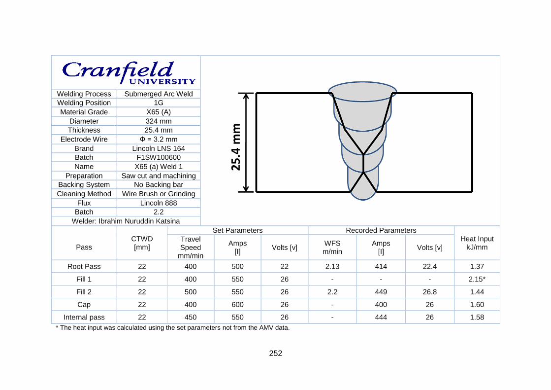
252

Welding Process Submerged Arc Weld

Welding Position 1G

Material Grade X65 (A)

Diameter 324 mm

Thickness 25.4 mm

Electrode Wire Ф = 3.2 mm

Brand Lincoln LNS 164

Batch F1SW100600

Name X65 (a) Weld 1

Preparation Saw cut and machining

Backing System No Backing bar

Cleaning Method Wire Brush or Grinding

Flux Lincoln 888

Batch 2.2

Welder: Ibrahim Nuruddin Katsina

Pass

CTWD [mm]

Set Parameters Recorded Parameters

Heat Input kJ/mm

Travel Speed

mm/min

Amps [I]

Volts [v] WFS m/min

Amps [I]

Volts [v]

Root Pass 22 400 500 22 2.13 414 22.4 1.37

Fill 1 22 400 550 26 - - - 2.15*

Fill 2 22 500 550 26 2.2 449 26.8 1.44

Cap 22 400 600 26 - 400 26 1.60

Internal pass 22 450 550 26 - 444 26 1.58

* The heat input was calculated using the set parameters not from the AMV data.

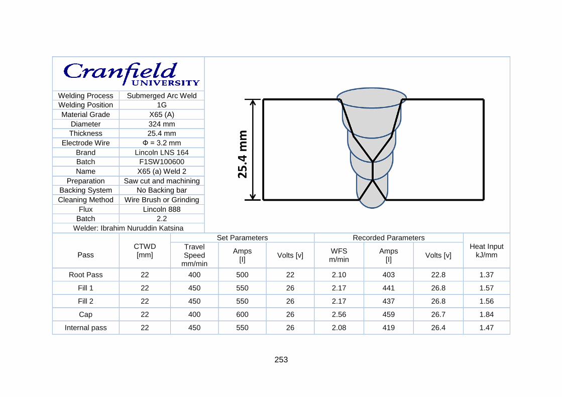
253

Welding Process Submerged Arc Weld

Welding Position 1G

Material Grade X65 (A)

Diameter 324 mm

Thickness 25.4 mm

Electrode Wire Ф = 3.2 mm

Brand Lincoln LNS 164

Batch F1SW100600

Name X65 (a) Weld 2

Preparation Saw cut and machining

Backing System No Backing bar

Cleaning Method Wire Brush or Grinding

Flux Lincoln 888

Batch 2.2

Welder: Ibrahim Nuruddin Katsina

Pass

CTWD [mm]

Set Parameters Recorded Parameters

Heat Input kJ/mm

Travel Speed

mm/min

Amps [I]

Volts [v] WFS m/min

Amps [I]

Volts [v]

Root Pass 22 400 500 22 2.10 403 22.8 1.37

Fill 1 22 450 550 26 2.17 441 26.8 1.57

Fill 2 22 450 550 26 2.17 437 26.8 1.56

Cap 22 400 600 26 2.56 459 26.7 1.84

Internal pass 22 450 550 26 2.08 419 26.4 1.47

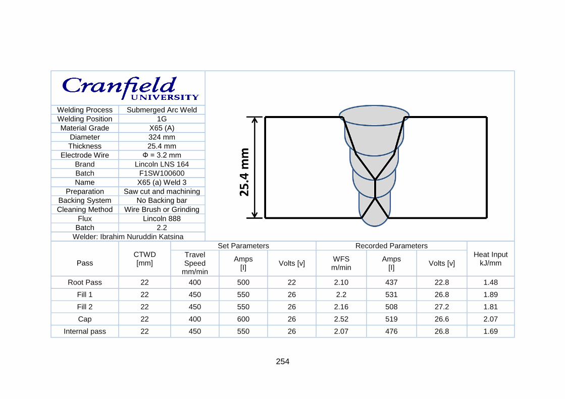
254

Welding Process Submerged Arc Weld

Welding Position 1G

Material Grade X65 (A)

Diameter 324 mm

Thickness 25.4 mm

Electrode Wire Ф = 3.2 mm

Brand Lincoln LNS 164

Batch F1SW100600

Name X65 (a) Weld 3

Preparation Saw cut and machining

Backing System No Backing bar

Cleaning Method Wire Brush or Grinding

Flux Lincoln 888

Batch 2.2

Welder: Ibrahim Nuruddin Katsina

Pass

CTWD [mm]

Set Parameters Recorded Parameters

Heat Input kJ/mm

Travel Speed

mm/min

Amps [I]

Volts [v] WFS m/min

Amps [I]

Volts [v]

Root Pass 22 400 500 22 2.10 437 22.8 1.48

Fill 1 22 450 550 26 2.2 531 26.8 1.89

Fill 2 22 450 550 26 2.16 508 27.2 1.81

Cap 22 400 600 26 2.52 519 26.6 2.07

Internal pass 22 450 550 26 2.07 476 26.8 1.69

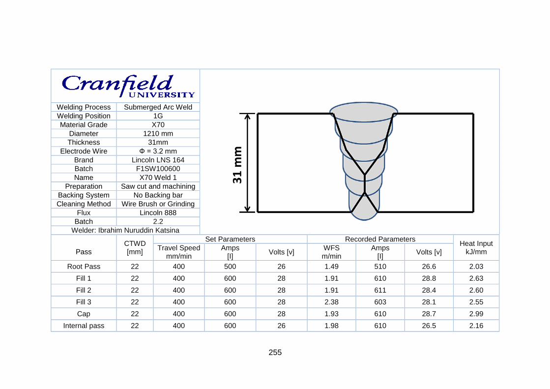
255

Welding Process Submerged Arc Weld

Welding Position 1G

Material Grade X70

Diameter 1210 mm

Thickness 31mm

Electrode Wire Ф = 3.2 mm

Brand Lincoln LNS 164

Batch F1SW100600

Name X70 Weld 1

Preparation Saw cut and machining

Backing System No Backing bar

Cleaning Method Wire Brush or Grinding

Flux Lincoln 888

Batch 2.2

Welder: Ibrahim Nuruddin Katsina

Pass

CTWD [mm]

Set Parameters Recorded Parameters Heat Input

kJ/mm Travel Speed

mm/min Amps

[I] Volts [v]

WFS m/min

Amps [I]

Volts [v]

Root Pass 22 400 500 26 1.49 510 26.6 2.03

Fill 1 22 400 600 28 1.91 610 28.8 2.63

Fill 2 22 400 600 28 1.91 611 28.4 2.60

Fill 3 22 400 600 28 2.38 603 28.1 2.55

Cap 22 400 600 28 1.93 610 28.7 2.99

Internal pass 22 400 600 26 1.98 610 26.5 2.16

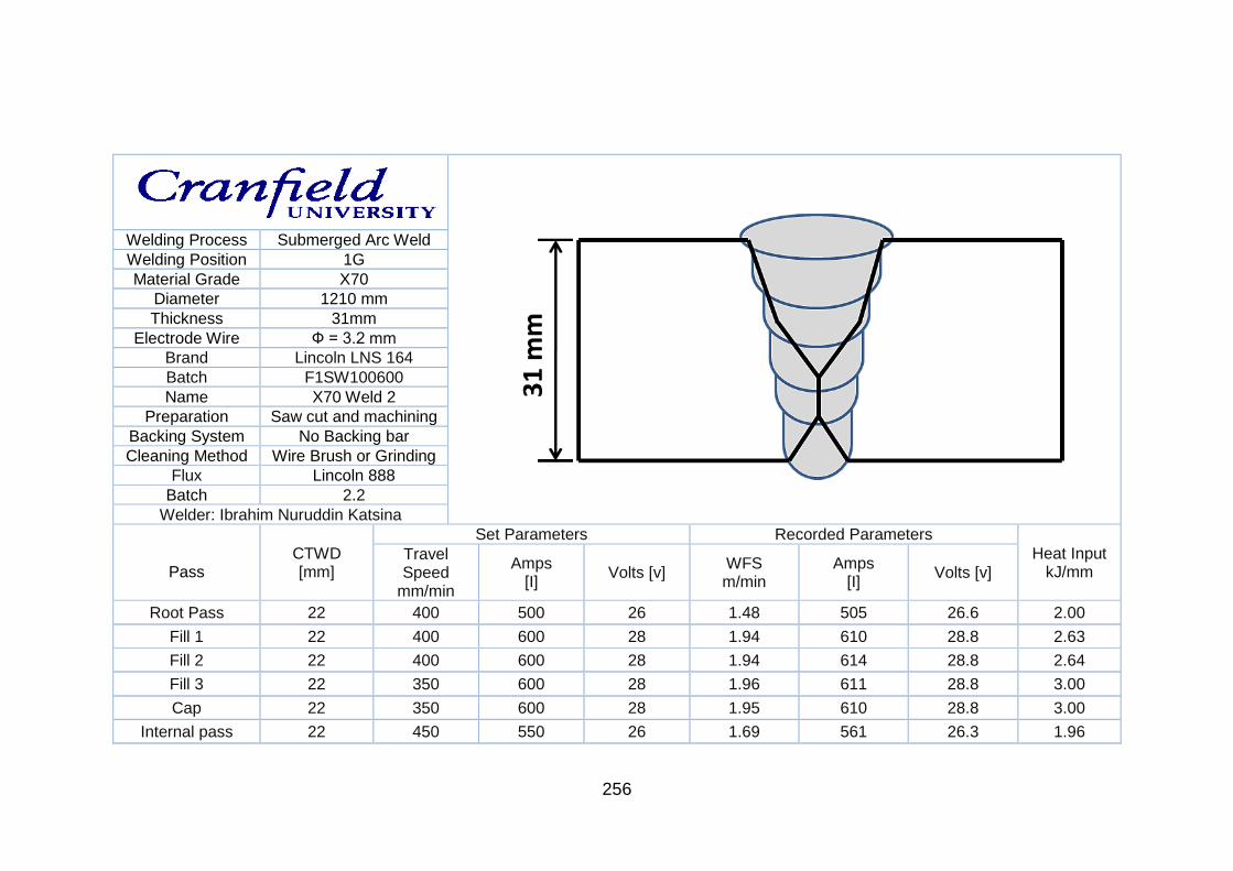
256

Welding Process Submerged Arc Weld

Welding Position 1G

Material Grade X70

Diameter 1210 mm

Thickness 31mm

Electrode Wire Ф = 3.2 mm

Brand Lincoln LNS 164

Batch F1SW100600

Name X70 Weld 2

Preparation Saw cut and machining

Backing System No Backing bar

Cleaning Method Wire Brush or Grinding

Flux Lincoln 888

Batch 2.2

Welder: Ibrahim Nuruddin Katsina

Pass

CTWD [mm]

Set Parameters Recorded Parameters

Heat Input kJ/mm

Travel Speed

mm/min

Amps [I]

Volts [v] WFS m/min

Amps [I]

Volts [v]

Root Pass 22 400 500 26 1.48 505 26.6 2.00

Fill 1 22 400 600 28 1.94 610 28.8 2.63

Fill 2 22 400 600 28 1.94 614 28.8 2.64

Fill 3 22 350 600 28 1.96 611 28.8 3.00

Cap 22 350 600 28 1.95 610 28.8 3.00

Internal pass 22 450 550 26 1.69 561 26.3 1.96

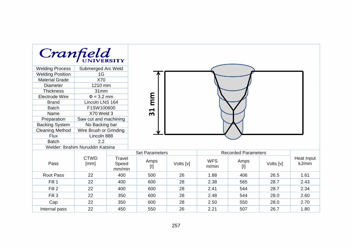
257

Welding Process Submerged Arc Weld

Welding Position 1G

Material Grade X70

Diameter 1210 mm

Thickness 31mm

Electrode Wire Ф = 3.2 mm

Brand Lincoln LNS 164

Batch F1SW100600

Name X70 Weld 3

Preparation Saw cut and machining

Backing System No Backing bar

Cleaning Method Wire Brush or Grinding

Flux Lincoln 888

Batch 2.2

Welder: Ibrahim Nuruddin Katsina

Pass

CTWD [mm]

Set Parameters Recorded Parameters

Heat Input kJ/mm

Travel Speed

mm/min

Amps [I]

Volts [v] WFS m/min

Amps [I]

Volts [v]

Root Pass 22 400 500 26 1.88 406 26.5 1.61

Fill 1 22 400 600 28 2.38 565 28.7 2.43

Fill 2 22 400 600 28 2.41 544 28.7 2.34

Fill 3 22 350 600 28 2.48 544 28.0 2.60

Cap 22 350 600 28 2.50 550 28.0 2.70

Internal pass 22 450 550 26 2.21 507 26.7 1.80

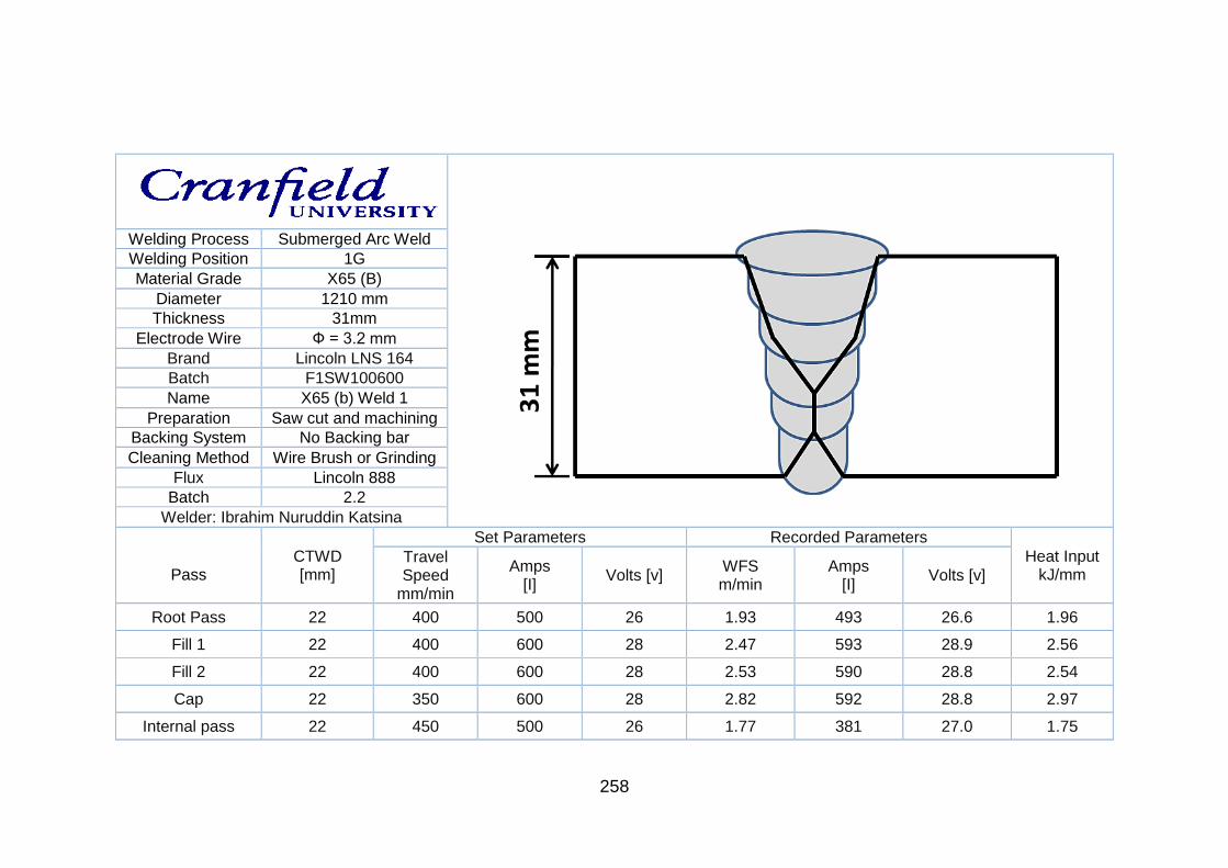
258

Welding Process Submerged Arc Weld

Welding Position 1G

Material Grade X65 (B)

Diameter 1210 mm

Thickness 31mm

Electrode Wire Ф = 3.2 mm

Brand Lincoln LNS 164

Batch F1SW100600

Name X65 (b) Weld 1

Preparation Saw cut and machining

Backing System No Backing bar

Cleaning Method Wire Brush or Grinding

Flux Lincoln 888

Batch 2.2

Welder: Ibrahim Nuruddin Katsina

Pass

CTWD [mm]

Set Parameters Recorded Parameters

Heat Input kJ/mm

Travel Speed

mm/min

Amps [I]

Volts [v] WFS m/min

Amps [I]

Volts [v]

Root Pass 22 400 500 26 1.93 493 26.6 1.96

Fill 1 22 400 600 28 2.47 593 28.9 2.56

Fill 2 22 400 600 28 2.53 590 28.8 2.54

Cap 22 350 600 28 2.82 592 28.8 2.97

Internal pass 22 450 500 26 1.77 381 27.0 1.75

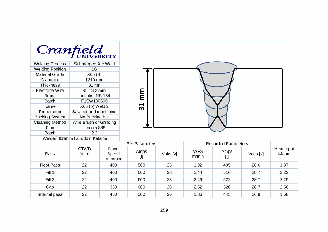
259

Welding Process Submerged Arc Weld

Welding Position 1G

Material Grade X65 (B)

Diameter 1210 mm

Thickness 31mm

Electrode Wire Ф = 3.2 mm

Brand Lincoln LNS 164

Batch F1SW100600

Name X65 (b) Weld 2

Preparation Saw cut and machining

Backing System No Backing bar

Cleaning Method Wire Brush or Grinding

Flux Lincoln 888

Batch 2.2

Welder: Ibrahim Nuruddin Katsina

Pass

CTWD [mm]

Set Parameters Recorded Parameters

Heat Input kJ/mm

Travel Speed

mm/min

Amps [I]

Volts [v] WFS m/min

Amps [I]

Volts [v]

Root Pass 22 400 500 26 1.92 495 26.6 1.97

Fill 1 22 400 600 28 2.44 516 28.7 2.22

Fill 2 22 400 600 28 2.49 522 28.7 2.25

Cap 22 350 600 28 2.52 520 28.7 2.56

Internal pass 22 450 500 26 1.88 445 26.8 1.58

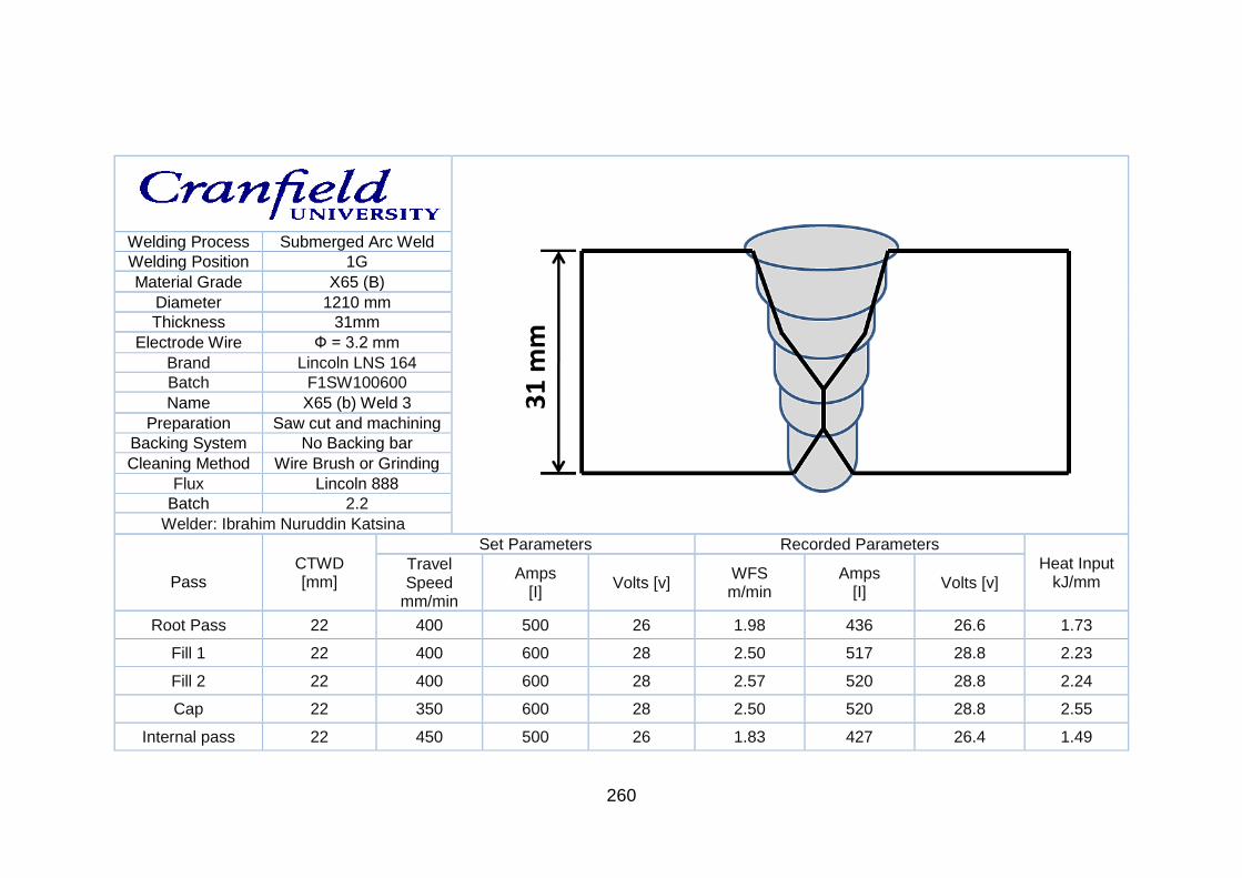
260

Welding Process Submerged Arc Weld

Welding Position 1G

Material Grade X65 (B)

Diameter 1210 mm

Thickness 31mm

Electrode Wire Ф = 3.2 mm

Brand Lincoln LNS 164

Batch F1SW100600

Name X65 (b) Weld 3

Preparation Saw cut and machining

Backing System No Backing bar

Cleaning Method Wire Brush or Grinding

Flux Lincoln 888

Batch 2.2

Welder: Ibrahim Nuruddin Katsina

Pass

CTWD [mm]

Set Parameters Recorded Parameters

Heat Input kJ/mm

Travel Speed

mm/min

Amps [I]

Volts [v] WFS m/min

Amps [I]

Volts [v]

Root Pass 22 400 500 26 1.98 436 26.6 1.73

Fill 1 22 400 600 28 2.50 517 28.8 2.23

Fill 2 22 400 600 28 2.57 520 28.8 2.24

Cap 22 350 600 28 2.50 520 28.8 2.55

Internal pass 22 450 500 26 1.83 427 26.4 1.49

261

A.2 Narrow groove Tandem MIG Weld Parameters

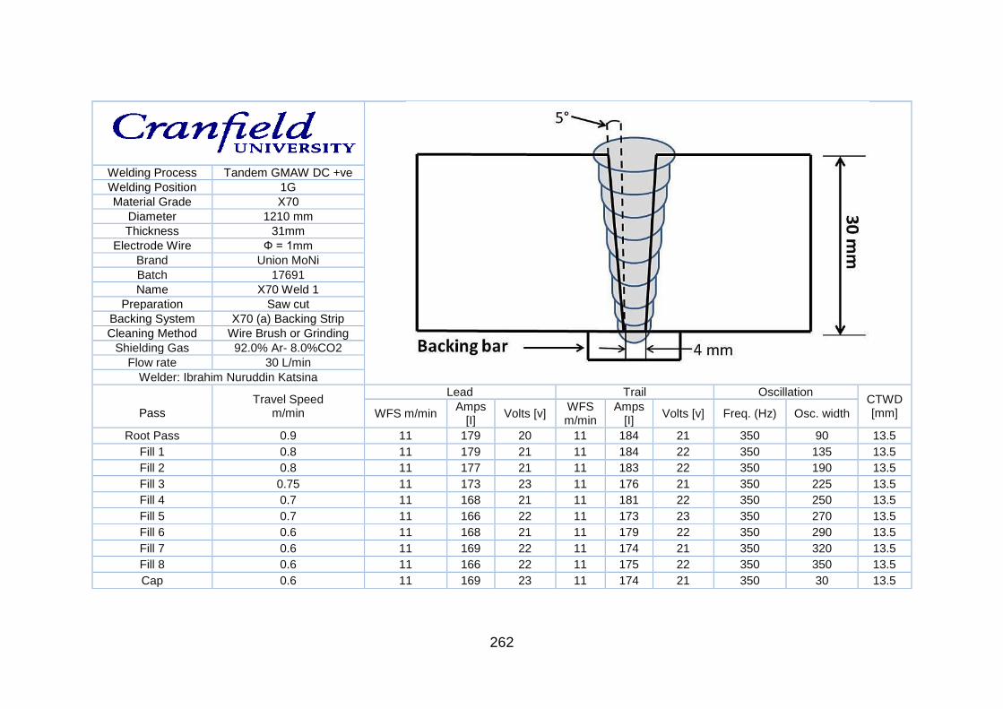
262

Welding Process Tandem GMAW DC +ve

Welding Position 1G

Material Grade X70

Diameter 1210 mm

Thickness 31mm

Electrode Wire Ф = 1mm

Brand Union MoNi

Batch 17691

Name X70 Weld 1

Preparation Saw cut

Backing System X70 (a) Backing Strip

Cleaning Method Wire Brush or Grinding

Shielding Gas 92.0% Ar- 8.0%CO2

Flow rate 30 L/min

Welder: Ibrahim Nuruddin Katsina

Pass

Travel Speed m/min

Lead Trail Oscillation CTWD [mm] WFS m/min

Amps [I]

Volts [v] WFS m/min

Amps [I]

Volts [v] Freq. (Hz) Osc. width

Root Pass 0.9 11 179 20 11 184 21 350 90 13.5

Fill 1 0.8 11 179 21 11 184 22 350 135 13.5

Fill 2 0.8 11 177 21 11 183 22 350 190 13.5

Fill 3 0.75 11 173 23 11 176 21 350 225 13.5

Fill 4 0.7 11 168 21 11 181 22 350 250 13.5

Fill 5 0.7 11 166 22 11 173 23 350 270 13.5

Fill 6 0.6 11 168 21 11 179 22 350 290 13.5

Fill 7 0.6 11 169 22 11 174 21 350 320 13.5

Fill 8 0.6 11 166 22 11 175 22 350 350 13.5

Cap 0.6 11 169 23 11 174 21 350 30 13.5

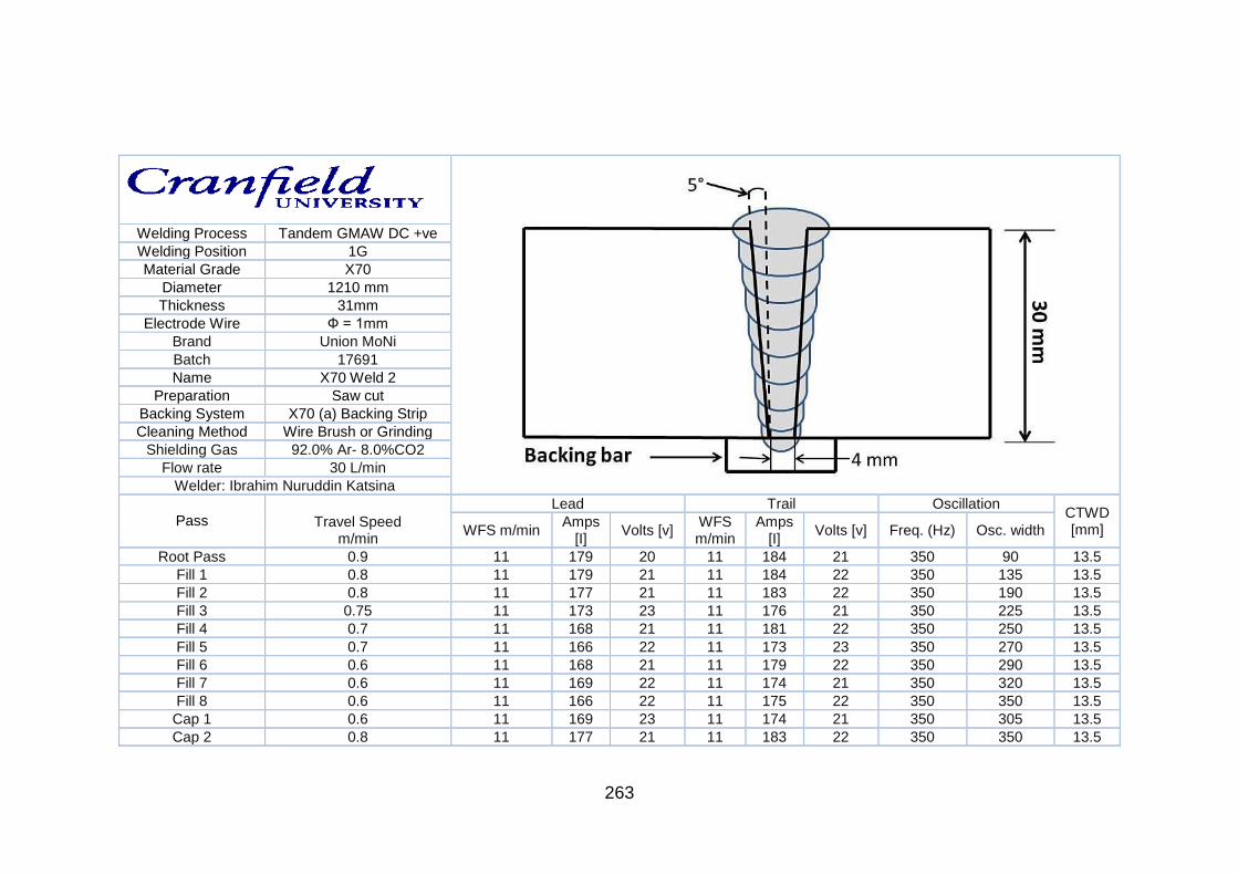
263

Welding Process Tandem GMAW DC +ve

Welding Position 1G

Material Grade X70

Diameter 1210 mm

Thickness 31mm

Electrode Wire Ф = 1mm

Brand Union MoNi

Batch 17691

Name X70 Weld 2

Preparation Saw cut

Backing System X70 (a) Backing Strip

Cleaning Method Wire Brush or Grinding

Shielding Gas 92.0% Ar- 8.0%CO2

Flow rate 30 L/min

Welder: Ibrahim Nuruddin Katsina

Pass Travel Speed

m/min

Lead Trail Oscillation CTWD [mm] WFS m/min

Amps [I]

Volts [v] WFS m/min

Amps [I]

Volts [v] Freq. (Hz) Osc. width

Root Pass 0.9 11 179 20 11 184 21 350 90 13.5

Fill 1 0.8 11 179 21 11 184 22 350 135 13.5

Fill 2 0.8 11 177 21 11 183 22 350 190 13.5

Fill 3 0.75 11 173 23 11 176 21 350 225 13.5

Fill 4 0.7 11 168 21 11 181 22 350 250 13.5

Fill 5 0.7 11 166 22 11 173 23 350 270 13.5

Fill 6 0.6 11 168 21 11 179 22 350 290 13.5

Fill 7 0.6 11 169 22 11 174 21 350 320 13.5

Fill 8 0.6 11 166 22 11 175 22 350 350 13.5

Cap 1 0.6 11 169 23 11 174 21 350 305 13.5

Cap 2 0.8 11 177 21 11 183 22 350 350 13.5

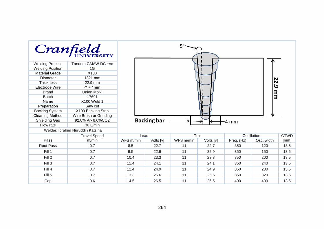
264

Welding Process Tandem GMAW DC +ve

Welding Position 1G

Material Grade X100

Diameter 1321 mm

Thickness 22.9 mm

Electrode Wire Ф = 1mm

Brand Union MoNi

Batch 17691

Name X100 Weld 1

Preparation Saw cut

Backing System X100 Backing Strip

Cleaning Method Wire Brush or Grinding

Shielding Gas 92.0% Ar- 8.0%CO2

Flow rate 30 L/min

Welder: Ibrahim Nuruddin Katsina

Pass

Travel Speed m/min

Lead Trail Oscillation CTWD [mm] WFS m/min Volts [v] WFS m/min Volts [v] Freq. (Hz) Osc. width

Root Pass 0.7 8.5 22.7 11 22.7 350 120 13.5

Fill 1 0.7 9.5 22.9 11 22.9 350 150 13.5

Fill 2 0.7 10.4 23.3 11 23.3 350 200 13.5

Fill 3 0.7 11.4 24.1 11 24.1 350 240 13.5

Fill 4 0.7 12.4 24.9 11 24.9 350 280 13.5

Fill 5 0.7 13.3 25.6 11 25.6 350 320 13.5

Cap 0.6 14.5 26.5 11 26.5 400 400 13.5

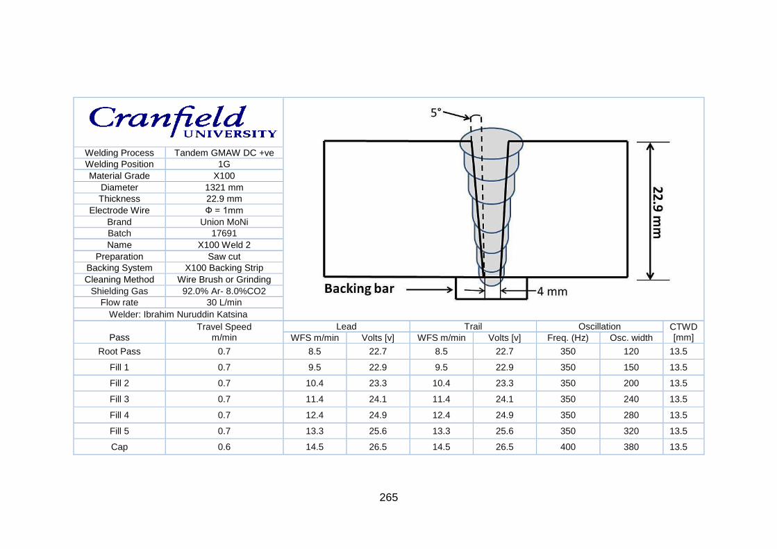
265

Welding Process Tandem GMAW DC +ve

Welding Position 1G

Material Grade X100

Diameter 1321 mm

Thickness 22.9 mm

Electrode Wire Ф = 1mm

Brand Union MoNi

Batch 17691

Name X100 Weld 2

Preparation Saw cut

Backing System X100 Backing Strip

Cleaning Method Wire Brush or Grinding

Shielding Gas 92.0% Ar- 8.0%CO2

Flow rate 30 L/min

Welder: Ibrahim Nuruddin Katsina

Pass

Travel Speed m/min

Lead Trail Oscillation CTWD [mm] WFS m/min Volts [v] WFS m/min Volts [v] Freq. (Hz) Osc. width

Root Pass 0.7 8.5 22.7 8.5 22.7 350 120 13.5

Fill 1 0.7 9.5 22.9 9.5 22.9 350 150 13.5

Fill 2 0.7 10.4 23.3 10.4 23.3 350 200 13.5

Fill 3 0.7 11.4 24.1 11.4 24.1 350 240 13.5

Fill 4 0.7 12.4 24.9 12.4 24.9 350 280 13.5

Fill 5 0.7 13.3 25.6 13.3 25.6 350 320 13.5

Cap 0.6 14.5 26.5 14.5 26.5 400 380 13.5

266

Appendix B Gleeble experiments thermal cycles

B.1 X70 first trial

267

X70 First Thermal Cycles Second Thermal Cycles Third Thermal Cycles Charpy Impact Energy (J)

No.

Heated

at

500°C/s

Cooled

at

50°C/s

to

Cooled

to (°C)

C R

(°C/sec)

Heated

at

500°C/s

to

Cooled

to (°C)

C R

(°C/sec)

Heated

at

500°C/s

to

Cooled

to (°C)

CR

(°C/sec) Quench 0°C

-

20°

C

-

40°

C

-

60°

C

-

80°

C

1 1250 800 200 25 800 200 25 - - - No 299 299 7 73 -

2 1250 800 200 40 800 200 40 - - - No - - 190 - -

3 1250 800 100 40 800 100 40 - - - No - - - 39 -

4 1250 900 200 25 900 200 25 - - - Air - 256 39 - -

5 1250 900 200 10 900 200 10 - - - Air - - 279 54 -

6 1250 850 200 40 850 200 40 - - - Air - - 264 - -

7 1250 850 200 25 850 200 25 - - - Air - - 245 222 -

8 1250 850 200 10 850 200 10 - - - Air - - 299 208 -

9 1250 800 200 40 800 200 40 - - - Air - - 295 - -

10 1250 800 200 25 800 200 25 - - - Air - 299 116 - -

11 1250 800 200 10 800 200 10 - - - Air - - 299 217 -

12 1250 800 20 25 800 20 25 450 20 25 Air - - 299 277 -

13 1250 800 20 10 800 20 10 450 20 10 Air - - 299 239 -

14 1250 800 20 25 800 20 25 350 20 25 Air - - 238 233 -

15 1250 800 20 10 800 20 10 350 20 10 Air - - 256 40 -

16 1250 750 200 40 750 200 40 - - - Air - - - 251 -

17 1250 750 200 25 750 200 25 - - - Air - - 225 217 -

18 1250 750 200 10 750 200 10 - - - Air - - 248 229 -

19 PARENT METAL

-

- 218 190 208 167

268

B.2 X70 second experiment

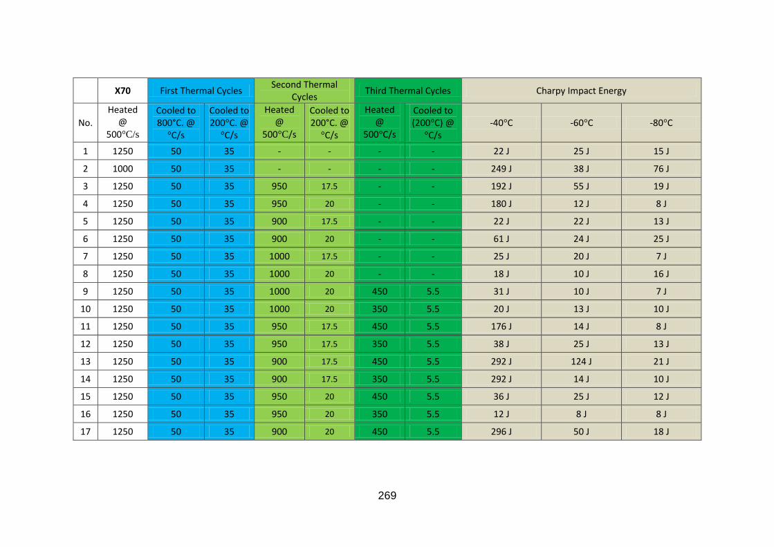
269

X70 First Thermal Cycles Second Thermal

Cycles Third Thermal Cycles Charpy Impact Energy

No.

Heated @

500°C/s

to

Cooled to 800°C. @

°C/s

Cooled to 200°C. @

°C/s

Heated @

500°C/s to

Cooled to 200°C. @

°C/s

Heated @

500°C/s to

Cooled to (200°C) @

°C/s -40°C -60°C -80°C

1 1250 50 35 - - - - 22 J 25 J 15 J

2 1000 50 35 - - - - 249 J 38 J 76 J

3 1250 50 35 950 17.5 - - 192 J 55 J 19 J

4 1250 50 35 950 20 - - 180 J 12 J 8 J

5 1250 50 35 900 17.5 - - 22 J 22 J 13 J

6 1250 50 35 900 20 - - 61 J 24 J 25 J

7 1250 50 35 1000 17.5 - - 25 J 20 J 7 J

8 1250 50 35 1000 20 - - 18 J 10 J 16 J

9 1250 50 35 1000 20 450 5.5 31 J 10 J 7 J

10 1250 50 35 1000 20 350 5.5 20 J 13 J 10 J

11 1250 50 35 950 17.5 450 5.5 176 J 14 J 8 J

12 1250 50 35 950 17.5 350 5.5 38 J 25 J 13 J

13 1250 50 35 900 17.5 450 5.5 292 J 124 J 21 J

14 1250 50 35 900 17.5 350 5.5 292 J 14 J 10 J

15 1250 50 35 950 20 450 5.5 36 J 25 J 12 J

16 1250 50 35 950 20 350 5.5 12 J 8 J 8 J

17 1250 50 35 900 20 450 5.5 296 J 50 J 18 J

270

B.3 X65 (B) and X65 (A) Gleeble experiments

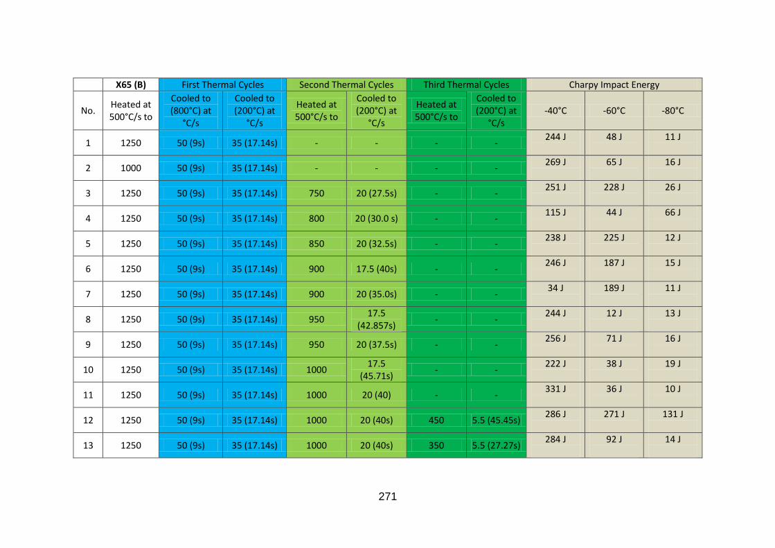
271

X65 (B) First Thermal Cycles Second Thermal Cycles Third Thermal Cycles Charpy Impact Energy

No. Heated at 500°C/s to

Cooled to (800°C) at

°C/s

Cooled to (200°C) at

°C/s

Heated at 500°C/s to

Cooled to (200°C) at

°C/s

Heated at 500°C/s to

Cooled to (200°C) at

°C/s -40°C -60°C -80°C

1 1250 50 (9s) 35 (17.14s) - - - - 244 J

48 J

11 J

2 1000 50 (9s) 35 (17.14s) - - - - 269 J

65 J

16 J

3 1250 50 (9s) 35 (17.14s) 750 20 (27.5s) - - 251 J

228 J

26 J

4 1250 50 (9s) 35 (17.14s) 800 20 (30.0 s) - - 115 J

44 J

66 J

5 1250 50 (9s) 35 (17.14s) 850 20 (32.5s) - - 238 J

225 J

12 J

6 1250 50 (9s) 35 (17.14s) 900 17.5 (40s) - - 246 J

187 J

15 J

7 1250 50 (9s) 35 (17.14s) 900 20 (35.0s) - - 34 J

189 J

11 J

8 1250 50 (9s) 35 (17.14s) 950 17.5

(42.857s) - -

244 J

12 J

13 J

9 1250 50 (9s) 35 (17.14s) 950 20 (37.5s) - - 256 J

71 J

16 J

10 1250 50 (9s) 35 (17.14s) 1000 17.5

(45.71s) - -

222 J

38 J

19 J

11 1250 50 (9s) 35 (17.14s) 1000 20 (40) - - 331 J

36 J

10 J

12 1250 50 (9s) 35 (17.14s) 1000 20 (40s) 450 5.5 (45.45s) 286 J

271 J

131 J

13 1250 50 (9s) 35 (17.14s) 1000 20 (40s) 350 5.5 (27.27s) 284 J

92 J

14 J

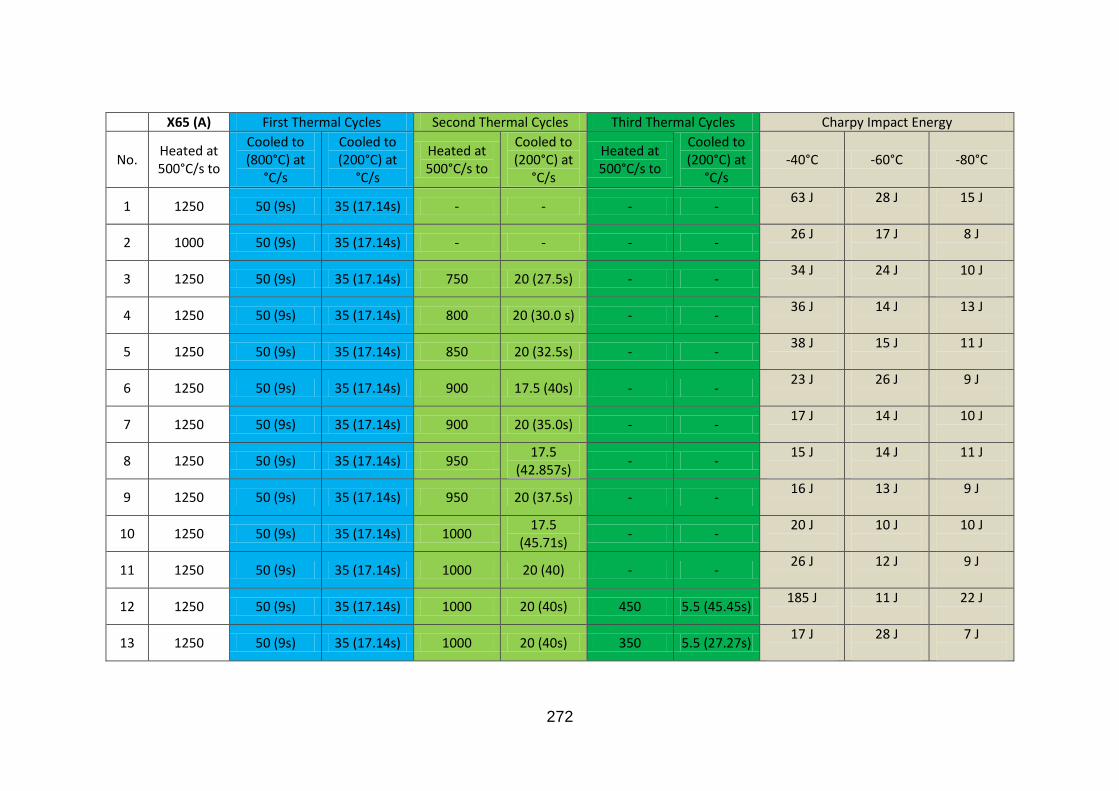
272

X65 (A) First Thermal Cycles Second Thermal Cycles Third Thermal Cycles Charpy Impact Energy

No. Heated at 500°C/s to

Cooled to (800°C) at

°C/s

Cooled to (200°C) at

°C/s

Heated at 500°C/s to

Cooled to (200°C) at

°C/s

Heated at 500°C/s to

Cooled to (200°C) at

°C/s -40°C -60°C -80°C

1 1250 50 (9s) 35 (17.14s) - - - - 63 J

28 J

15 J

2 1000 50 (9s) 35 (17.14s) - - - - 26 J

17 J

8 J

3 1250 50 (9s) 35 (17.14s) 750 20 (27.5s) - - 34 J

24 J

10 J

4 1250 50 (9s) 35 (17.14s) 800 20 (30.0 s) - - 36 J

14 J

13 J

5 1250 50 (9s) 35 (17.14s) 850 20 (32.5s) - - 38 J

15 J

11 J

6 1250 50 (9s) 35 (17.14s) 900 17.5 (40s) - - 23 J

26 J

9 J

7 1250 50 (9s) 35 (17.14s) 900 20 (35.0s) - - 17 J

14 J

10 J

8 1250 50 (9s) 35 (17.14s) 950 17.5

(42.857s) - -

15 J

14 J

11 J

9 1250 50 (9s) 35 (17.14s) 950 20 (37.5s) - - 16 J

13 J

9 J

10 1250 50 (9s) 35 (17.14s) 1000 17.5

(45.71s) - -

20 J

10 J

10 J

11 1250 50 (9s) 35 (17.14s) 1000 20 (40) - - 26 J

12 J

9 J

12 1250 50 (9s) 35 (17.14s) 1000 20 (40s) 450 5.5 (45.45s) 185 J

11 J

22 J

13 1250 50 (9s) 35 (17.14s) 1000 20 (40s) 350 5.5 (27.27s) 17 J

28 J

7 J

273

Appendix C MATLAB Programs

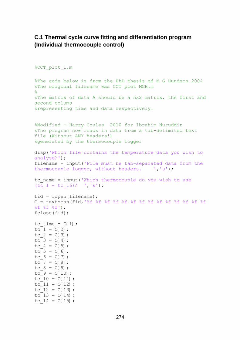
274

C.1 Thermal cycle curve fitting and differentiation program

(Individual thermocouple control)

%CCT_plot_1.m

%The code below is from the PhD thesis of M G Hundson 2004

%The original filename was CCT_plot_MGH.m

%

%The matrix of data A should be a nx2 matrix, the first and

second colums

%representing time and data respectively.

%Modified - Harry Coules 2010 for Ibrahim Nuruddin

%The program now reads in data from a tab-delimited text

file (Without ANY headers!)

%generated by the thermocouple logger

disp('Which file contains the temperature data you wish to

analyse?');

filename = input('File must be tab-separated data from the

thermocouple logger, without headers. ','s');

tc_name = input('Which thermocouple do you wish to use

(tc_1 - tc_16)? ','s');

fid = fopen(filename);

C = textscan(fid,'%f %f %f %f %f %f %f %f %f %f %f %f %f %f

%f %f %f');

fclose(fid);

tc_time = C{1};

tc_1 = C{2};

tc_2 = C{3};

tc_3 = C{4};

tc_4 = C{5};

tc_5 = C{6};

tc_6 = C{7};

tc_7 = C{8};

tc_8 = C{9};

tc_9 = C{10};

tc_10 = C{11};

tc_11 = C{12};

tc_12 = C{13};

tc_13 = C{14};

tc_14 = C{15};

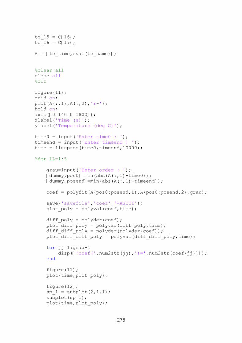
275

tc_15 = C{16};

tc_16 = C{17};

A = [tc_time,eval(tc_name)];

%clear all

close all

%clc

figure(11);

grid on;

plot(A(:,1),A(:,2),'r-');

hold on;

axis([0 140 0 1800]);

xlabel('Time (s)');

ylabel('Temperature (deg C)');

time0 = input('Enter time0 : ');

timeend = input('Enter timeend : ');

time = linspace(time0,timeend,10000);

%for LL=1:5

grau=input('Enter order : ');

[dummy,pos0]=min(abs(A(:,1)-time0));

[dummy,posend]=min(abs(A(:,1)-timeend));

coef = polyfit(A(pos0:posend,1),A(pos0:posend,2),grau);

save('savefile','coef','-ASCII');

plot_poly = polyval(coef,time);

diff_poly = polyder(coef);

plot_diff_poly = polyval(diff_poly,time);

diff_diff_poly = polyder(polyder(coef));

plot_diff_diff_poly = polyval(diff_diff_poly,time);

for jj=1:grau+1

disp(['coef(',num2str(jj),')=',num2str(coef(jj))]);

end

figure(11);

plot(time,plot_poly);

figure(12);

sp_1 = subplot(2,1,1);

subplot(sp_1);

plot(time,plot_poly);

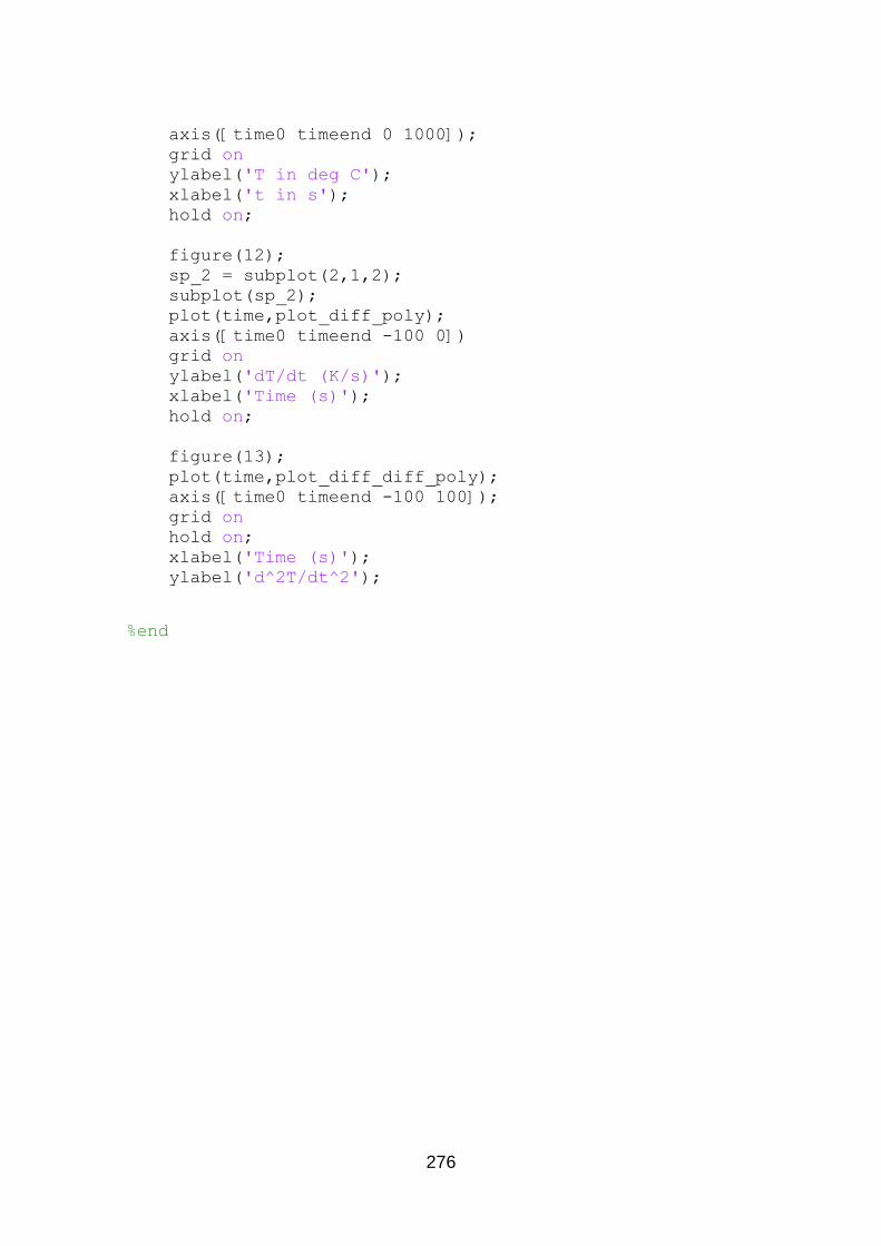
276

axis([time0 timeend 0 1000]);

grid on

ylabel('T in deg C');

xlabel('t in s');

hold on;

figure(12);

sp_2 = subplot(2,1,2);

subplot(sp_2);

plot(time,plot_diff_poly);

axis([time0 timeend -100 0])

grid on

ylabel('dT/dt (K/s)');

xlabel('Time (s)');

hold on;

figure(13);

plot(time,plot_diff_diff_poly);

axis([time0 timeend -100 100]);

grid on

hold on;

xlabel('Time (s)');

ylabel('d^2T/dt^2');

%end

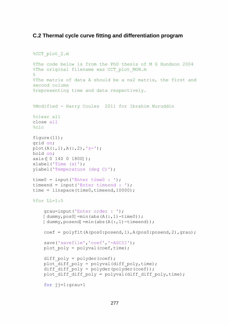
277

C.2 Thermal cycle curve fitting and differentiation program

%CCT_plot_2.m

%The code below is from the PhD thesis of M G Hundson 2004

%The original filename was CCT_plot_MGH.m

%

%The matrix of data A should be a nx2 matrix, the first and

second colums

%representing time and data respectively.

%Modified - Harry Coules 2011 for Ibrahim Nuruddin

%clear all

close all

%clc

figure(11);

grid on;

plot(A(:,1),A(:,2),'r-');

hold on;

axis([0 140 0 1800]);

xlabel('Time (s)');

ylabel('Temperature (deg C)');

time0 = input('Enter time0 : ');

timeend = input('Enter timeend : ');

time = linspace(time0,timeend,10000);

%for LL=1:5

grau=input('Enter order : ');

[dummy,pos0]=min(abs(A(:,1)-time0));

[dummy,posend]=min(abs(A(:,1)-timeend));

coef = polyfit(A(pos0:posend,1),A(pos0:posend,2),grau);

save('savefile','coef','-ASCII');

plot_poly = polyval(coef,time);

diff_poly = polyder(coef);

plot_diff_poly = polyval(diff_poly,time);

diff_diff_poly = polyder(polyder(coef));

plot_diff_diff_poly = polyval(diff_diff_poly,time);

for jj=1:grau+1

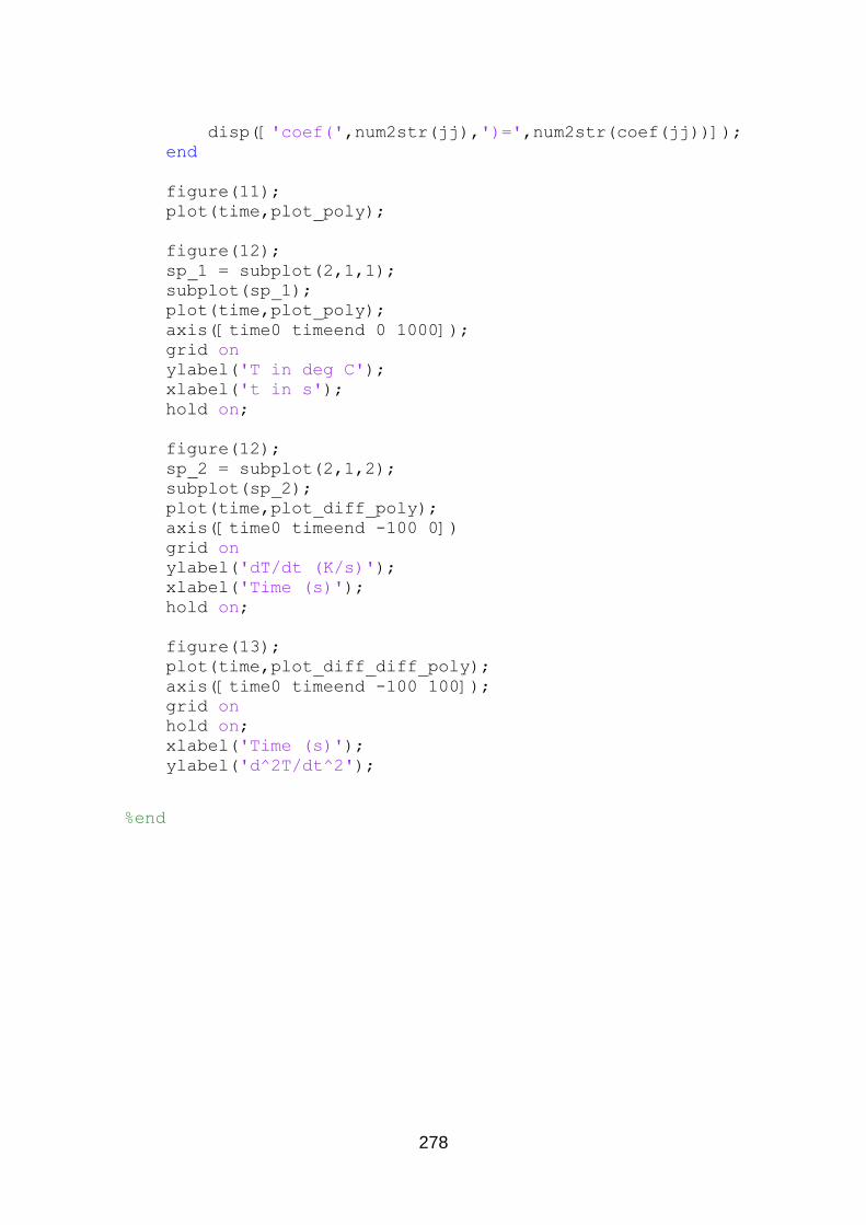
278

disp(['coef(',num2str(jj),')=',num2str(coef(jj))]);

end

figure(11);

plot(time,plot_poly);

figure(12);

sp_1 = subplot(2,1,1);

subplot(sp_1);

plot(time,plot_poly);

axis([time0 timeend 0 1000]);

grid on

ylabel('T in deg C');

xlabel('t in s');

hold on;

figure(12);

sp_2 = subplot(2,1,2);

subplot(sp_2);

plot(time,plot_diff_poly);

axis([time0 timeend -100 0])

grid on

ylabel('dT/dt (K/s)');

xlabel('Time (s)');

hold on;

figure(13);

plot(time,plot_diff_diff_poly);

axis([time0 timeend -100 100]);

grid on

hold on;

xlabel('Time (s)');

ylabel('d^2T/dt^2');

%end