IBM Eserver pSeries Sizing and Capacity Planning - IBM Redbooks

ibm.com/redbooks

IBM Eserver pSeries Sizing and Capacity PlanningA Practical Guide

G. Benton GibbsJerry M. Enriquez

Nigel GriffithsCorneliu Holban

Eunyoung KoYohichi Kurasawa

Discover the concepts and approach to perform sizing and capacity planning

Learn how to size the new systems

Understand capacity planning and upgrades

Front cover

http://www.redbooks.ibm.com/


IBM Eserver pSeries Sizing and Capacity Planning: A Practical Guide

March 2004

International Technical Support Organization

SG24-7071-00

© Copyright International Business Machines Corporation 2004. All rights reserved.Note to U.S. Government Users Restricted Rights -- Use, duplication or disclosure restricted by GSA ADPSchedule Contract with IBM Corp.

First Edition (March 2004)

This edition applies to the sizing and capacity planning of IBM Eserver pSeries and RS/6000 servers as configured and used with AIX 5L and Linux operating systems.

Note: Before using this information and the product it supports, read the information in “Notices” on page xi.

Contents

Notices . . . . . . . . . . . . . . . . . . . . . . . . . . . . . . . . . . . . . . . . . . . . . . . . . . . . . . . xiTrademarks . . . . . . . . . . . . . . . . . . . . . . . . . . . . . . . . . . . . . . . . . . . . . . . . . . . xii

Preface . . . . . . . . . . . . . . . . . . . . . . . . . . . . . . . . . . . . . . . . . . . . . . . . . . . . . . xiiiThe team that wrote this redbook. . . . . . . . . . . . . . . . . . . . . . . . . . . . . . . . . . . xiiiBecome a published author . . . . . . . . . . . . . . . . . . . . . . . . . . . . . . . . . . . . . . xviiComments welcome. . . . . . . . . . . . . . . . . . . . . . . . . . . . . . . . . . . . . . . . . . . . xviii

Part 1. Introduction to sizing and capacity planning. . . . . . . . . . . . . . . . . . . . . . . . . . . . . . . 1

Chapter 1. Overview, concepts, and approach. . . . . . . . . . . . . . . . . . . . . . . 31.1 Definitions of common terms. . . . . . . . . . . . . . . . . . . . . . . . . . . . . . . . . . . . 41.2 Concepts . . . . . . . . . . . . . . . . . . . . . . . . . . . . . . . . . . . . . . . . . . . . . . . . . . . 4

1.2.1 Required knowledge and experience . . . . . . . . . . . . . . . . . . . . . . . . . 51.2.2 Sizing with capacity planning . . . . . . . . . . . . . . . . . . . . . . . . . . . . . . . 51.2.3 The sizing problem . . . . . . . . . . . . . . . . . . . . . . . . . . . . . . . . . . . . . . . 51.2.4 Sizing inputs . . . . . . . . . . . . . . . . . . . . . . . . . . . . . . . . . . . . . . . . . . . . 61.2.5 Sizing outputs . . . . . . . . . . . . . . . . . . . . . . . . . . . . . . . . . . . . . . . . . . . 71.2.6 Who performs sizing . . . . . . . . . . . . . . . . . . . . . . . . . . . . . . . . . . . . . . 9

1.3 Sizing and resizing process. . . . . . . . . . . . . . . . . . . . . . . . . . . . . . . . . . . . . 91.3.1 System design and requirements . . . . . . . . . . . . . . . . . . . . . . . . . . . 101.3.2 Sizing model . . . . . . . . . . . . . . . . . . . . . . . . . . . . . . . . . . . . . . . . . . . 101.3.3 Hardware requirements. . . . . . . . . . . . . . . . . . . . . . . . . . . . . . . . . . . 111.3.4 Building block choices. . . . . . . . . . . . . . . . . . . . . . . . . . . . . . . . . . . . 111.3.5 eConfig for the price . . . . . . . . . . . . . . . . . . . . . . . . . . . . . . . . . . . . . 131.3.6 Sales, purchase, install, and production . . . . . . . . . . . . . . . . . . . . . . 131.3.7 Gathering performance data . . . . . . . . . . . . . . . . . . . . . . . . . . . . . . . 131.3.8 Performance tuning. . . . . . . . . . . . . . . . . . . . . . . . . . . . . . . . . . . . . . 131.3.9 Estimated or measured growth . . . . . . . . . . . . . . . . . . . . . . . . . . . . . 141.3.10 Capacity planning . . . . . . . . . . . . . . . . . . . . . . . . . . . . . . . . . . . . . . 141.3.11 Resizing model . . . . . . . . . . . . . . . . . . . . . . . . . . . . . . . . . . . . . . . . 141.3.12 rPerf reliance. . . . . . . . . . . . . . . . . . . . . . . . . . . . . . . . . . . . . . . . . . 15

1.4 Weighing sizing components. . . . . . . . . . . . . . . . . . . . . . . . . . . . . . . . . . . 161.4.1 Memory size . . . . . . . . . . . . . . . . . . . . . . . . . . . . . . . . . . . . . . . . . . . 161.4.2 Disk type and number . . . . . . . . . . . . . . . . . . . . . . . . . . . . . . . . . . . . 171.4.3 Adapters for disk, tape and network . . . . . . . . . . . . . . . . . . . . . . . . . 171.4.4 Software . . . . . . . . . . . . . . . . . . . . . . . . . . . . . . . . . . . . . . . . . . . . . . 171.4.5 Summary. . . . . . . . . . . . . . . . . . . . . . . . . . . . . . . . . . . . . . . . . . . . . . 18

1.5 The importance of the right amount of information . . . . . . . . . . . . . . . . . . 18

© Copyright IBM Corp. 2004. All rights reserved. iii

1.5.1 Brain overload . . . . . . . . . . . . . . . . . . . . . . . . . . . . . . . . . . . . . . . . . . 191.5.2 Summary. . . . . . . . . . . . . . . . . . . . . . . . . . . . . . . . . . . . . . . . . . . . . . 21

1.6 A practical sizing method . . . . . . . . . . . . . . . . . . . . . . . . . . . . . . . . . . . . . 211.6.1 Segmentation . . . . . . . . . . . . . . . . . . . . . . . . . . . . . . . . . . . . . . . . . . 21

1.7 Performance theory. . . . . . . . . . . . . . . . . . . . . . . . . . . . . . . . . . . . . . . . . . 251.8 General rules of thumb for RDBMS memory. . . . . . . . . . . . . . . . . . . . . . . 27

1.8.1 Application resident set . . . . . . . . . . . . . . . . . . . . . . . . . . . . . . . . . . . 271.8.2 RDBMS data and file system cache . . . . . . . . . . . . . . . . . . . . . . . . . 281.8.3 RDBMS utilization rules of thumb . . . . . . . . . . . . . . . . . . . . . . . . . . . 281.8.4 Utilization. . . . . . . . . . . . . . . . . . . . . . . . . . . . . . . . . . . . . . . . . . . . . . 291.8.5 RDBMS raw data to disk rules of thumb . . . . . . . . . . . . . . . . . . . . . . 301.8.6 RDBMS disk use rules of thumb . . . . . . . . . . . . . . . . . . . . . . . . . . . . 32

1.9 The performance saturation curve . . . . . . . . . . . . . . . . . . . . . . . . . . . . . . 321.10 Successive approximation and sizing levels . . . . . . . . . . . . . . . . . . . . . . 351.11 Plagiarism . . . . . . . . . . . . . . . . . . . . . . . . . . . . . . . . . . . . . . . . . . . . . . . . 361.12 Triangulation . . . . . . . . . . . . . . . . . . . . . . . . . . . . . . . . . . . . . . . . . . . . . . 37

1.12.1 A triangulation story . . . . . . . . . . . . . . . . . . . . . . . . . . . . . . . . . . . . 391.13 Common sizing mistakes . . . . . . . . . . . . . . . . . . . . . . . . . . . . . . . . . . . . 40

1.13.1 Sizing report outline . . . . . . . . . . . . . . . . . . . . . . . . . . . . . . . . . . . . 411.13.2 A sizing story. . . . . . . . . . . . . . . . . . . . . . . . . . . . . . . . . . . . . . . . . . 41

1.14 The eConfig configurator. . . . . . . . . . . . . . . . . . . . . . . . . . . . . . . . . . . . . 421.14.1 Configurator test . . . . . . . . . . . . . . . . . . . . . . . . . . . . . . . . . . . . . . . 43

1.15 Cost-based sizing method. . . . . . . . . . . . . . . . . . . . . . . . . . . . . . . . . . . . 451.16 High availability and disaster recovery . . . . . . . . . . . . . . . . . . . . . . . . . . 451.17 Capacity Upgrade on Demand . . . . . . . . . . . . . . . . . . . . . . . . . . . . . . . . 471.18 Sizing for Linux on pSeries . . . . . . . . . . . . . . . . . . . . . . . . . . . . . . . . . . . 48

Part 2. Components involved in sizing and capacity planning. . . . . . . . . . . . . . . . . . . . . . 51

Chapter 2. Hardware components . . . . . . . . . . . . . . . . . . . . . . . . . . . . . . . . 532.1 Performance methodology . . . . . . . . . . . . . . . . . . . . . . . . . . . . . . . . . . . . 542.2 Overview of pSeries systems . . . . . . . . . . . . . . . . . . . . . . . . . . . . . . . . . . 57

2.2.1 Autonomic computing . . . . . . . . . . . . . . . . . . . . . . . . . . . . . . . . . . . . 592.2.2 e-business on demand . . . . . . . . . . . . . . . . . . . . . . . . . . . . . . . . . . . 602.2.3 Reliability, availability, and serviceability features. . . . . . . . . . . . . . . 622.2.4 Capacity Upgrade on Demand . . . . . . . . . . . . . . . . . . . . . . . . . . . . . 64

2.3 pSeries processors . . . . . . . . . . . . . . . . . . . . . . . . . . . . . . . . . . . . . . . . . . 662.3.1 Processor descriptions . . . . . . . . . . . . . . . . . . . . . . . . . . . . . . . . . . . 682.3.2 RISC/CISC concepts. . . . . . . . . . . . . . . . . . . . . . . . . . . . . . . . . . . . . 682.3.3 Superscalar architecture: Pipelines and parallelisms . . . . . . . . . . . . 702.3.4 32-bit versus 64-bit computing . . . . . . . . . . . . . . . . . . . . . . . . . . . . . 712.3.5 Performance of processors . . . . . . . . . . . . . . . . . . . . . . . . . . . . . . . . 722.3.6 Processor evolution. . . . . . . . . . . . . . . . . . . . . . . . . . . . . . . . . . . . . . 74

iv IBM Eserver pSeries Sizing and Capacity Planning

2.4 Memory . . . . . . . . . . . . . . . . . . . . . . . . . . . . . . . . . . . . . . . . . . . . . . . . . . . 842.4.1 Memory hierarchy . . . . . . . . . . . . . . . . . . . . . . . . . . . . . . . . . . . . . . . 842.4.2 Locality concept . . . . . . . . . . . . . . . . . . . . . . . . . . . . . . . . . . . . . . . . 862.4.3 Caches . . . . . . . . . . . . . . . . . . . . . . . . . . . . . . . . . . . . . . . . . . . . . . . 872.4.4 Memory cycles . . . . . . . . . . . . . . . . . . . . . . . . . . . . . . . . . . . . . . . . . 902.4.5 Virtual memory concepts. . . . . . . . . . . . . . . . . . . . . . . . . . . . . . . . . . 912.4.6 Memory affinity . . . . . . . . . . . . . . . . . . . . . . . . . . . . . . . . . . . . . . . . . 942.4.7 Large page support . . . . . . . . . . . . . . . . . . . . . . . . . . . . . . . . . . . . . . 95

2.5 Input/output . . . . . . . . . . . . . . . . . . . . . . . . . . . . . . . . . . . . . . . . . . . . . . . . 972.5.1 Peripheral Component Interconnect . . . . . . . . . . . . . . . . . . . . . . . . . 982.5.2 PCI-X. . . . . . . . . . . . . . . . . . . . . . . . . . . . . . . . . . . . . . . . . . . . . . . . 101

2.6 Storage architectures . . . . . . . . . . . . . . . . . . . . . . . . . . . . . . . . . . . . . . . 1012.6.1 Direct access storage . . . . . . . . . . . . . . . . . . . . . . . . . . . . . . . . . . . 1032.6.2 Storage area networks . . . . . . . . . . . . . . . . . . . . . . . . . . . . . . . . . . 1092.6.3 Network-attached storage . . . . . . . . . . . . . . . . . . . . . . . . . . . . . . . . 1162.6.4 RAID . . . . . . . . . . . . . . . . . . . . . . . . . . . . . . . . . . . . . . . . . . . . . . . . 1222.6.5 IBM TotalStorage Enterprise Storage Server . . . . . . . . . . . . . . . . . 1332.6.6 IBM TotalStorage Fibre Array Storage Technology . . . . . . . . . . . . 1352.6.7 IBM 7133 Serial Disk System . . . . . . . . . . . . . . . . . . . . . . . . . . . . . 1372.6.8 IBM TotalStorage Expandable Storage Plus 320 . . . . . . . . . . . . . . 1382.6.9 The IBM TotalStorage Network Attached Storage . . . . . . . . . . . . . 139

2.7 Additional hardware considerations . . . . . . . . . . . . . . . . . . . . . . . . . . . . 1452.7.1 Multiprocessor configurations . . . . . . . . . . . . . . . . . . . . . . . . . . . . . 1452.7.2 NUMA . . . . . . . . . . . . . . . . . . . . . . . . . . . . . . . . . . . . . . . . . . . . . . . 1472.7.3 Logical partitioning . . . . . . . . . . . . . . . . . . . . . . . . . . . . . . . . . . . . . 1492.7.4 Dynamic logical partitioning (5.2.0) . . . . . . . . . . . . . . . . . . . . . . . . . 1532.7.5 Dynamic CPU sparing and CPU Guard (5.2.0). . . . . . . . . . . . . . . . 1582.7.6 UE-Gard (5.2.0). . . . . . . . . . . . . . . . . . . . . . . . . . . . . . . . . . . . . . . . 160

Chapter 3. Software components . . . . . . . . . . . . . . . . . . . . . . . . . . . . . . . 1633.1 AIX. . . . . . . . . . . . . . . . . . . . . . . . . . . . . . . . . . . . . . . . . . . . . . . . . . . . . . 164

3.1.1 History of AIX . . . . . . . . . . . . . . . . . . . . . . . . . . . . . . . . . . . . . . . . . 1643.1.2 AIX kernel . . . . . . . . . . . . . . . . . . . . . . . . . . . . . . . . . . . . . . . . . . . . 1693.1.3 Modes of operation (execution modes). . . . . . . . . . . . . . . . . . . . . . 1713.1.4 AIX 5L kernel subsystems. . . . . . . . . . . . . . . . . . . . . . . . . . . . . . . . 1713.1.5 Multitasking and multithreading support . . . . . . . . . . . . . . . . . . . . . 1743.1.6 64-bit kernel . . . . . . . . . . . . . . . . . . . . . . . . . . . . . . . . . . . . . . . . . . 177

3.2 Workload Manager . . . . . . . . . . . . . . . . . . . . . . . . . . . . . . . . . . . . . . . . . 1783.2.1 Classes . . . . . . . . . . . . . . . . . . . . . . . . . . . . . . . . . . . . . . . . . . . . . . 1793.2.2 Tiers . . . . . . . . . . . . . . . . . . . . . . . . . . . . . . . . . . . . . . . . . . . . . . . . 1833.2.3 Class attributes . . . . . . . . . . . . . . . . . . . . . . . . . . . . . . . . . . . . . . . . 184

3.3 Linux . . . . . . . . . . . . . . . . . . . . . . . . . . . . . . . . . . . . . . . . . . . . . . . . . . . . 1843.3.1 Linux for pSeries . . . . . . . . . . . . . . . . . . . . . . . . . . . . . . . . . . . . . . . 185

Contents v

3.3.2 Linux and AIX . . . . . . . . . . . . . . . . . . . . . . . . . . . . . . . . . . . . . . . . . 1853.3.3 Logical partitioning . . . . . . . . . . . . . . . . . . . . . . . . . . . . . . . . . . . . . 1863.3.4 Other related information and links . . . . . . . . . . . . . . . . . . . . . . . . . 186

Chapter 4. Benchmarks . . . . . . . . . . . . . . . . . . . . . . . . . . . . . . . . . . . . . . . 1874.1 Introduction to benchmarks . . . . . . . . . . . . . . . . . . . . . . . . . . . . . . . . . . . 1884.2 OLTP benchmarks . . . . . . . . . . . . . . . . . . . . . . . . . . . . . . . . . . . . . . . . . 189

4.2.1 TPC-C benchmark . . . . . . . . . . . . . . . . . . . . . . . . . . . . . . . . . . . . . 1894.3 Business intelligence benchmarks . . . . . . . . . . . . . . . . . . . . . . . . . . . . . 191

4.3.1 TPC-H benchmark . . . . . . . . . . . . . . . . . . . . . . . . . . . . . . . . . . . . . 1924.4 e-business benchmarks . . . . . . . . . . . . . . . . . . . . . . . . . . . . . . . . . . . . . 195

4.4.1 TPC-W benchmark . . . . . . . . . . . . . . . . . . . . . . . . . . . . . . . . . . . . . 1954.4.2 SPEC JBB2000 benchmark . . . . . . . . . . . . . . . . . . . . . . . . . . . . . . 1974.4.3 SPECweb99 benchmark . . . . . . . . . . . . . . . . . . . . . . . . . . . . . . . . . 199

4.5 High Performance Computing benchmarks . . . . . . . . . . . . . . . . . . . . . . 2024.5.1 SPEC CPU2000 benchmark . . . . . . . . . . . . . . . . . . . . . . . . . . . . . . 2034.5.2 LINPACK benchmark . . . . . . . . . . . . . . . . . . . . . . . . . . . . . . . . . . . 205

4.6 ISV benchmarks . . . . . . . . . . . . . . . . . . . . . . . . . . . . . . . . . . . . . . . . . . . 2064.6.1 SAP Standard Application benchmarks . . . . . . . . . . . . . . . . . . . . . 2064.6.2 Oracle Applications Standard benchmark. . . . . . . . . . . . . . . . . . . . 2104.6.3 Siebel platform sizing and performance program benchmark. . . . . 212

4.7 Relative performance . . . . . . . . . . . . . . . . . . . . . . . . . . . . . . . . . . . . . . . 214

Part 3. Sizing pSeries systems . . . . . . . . . . . . . . . . . . . . . . . . . . . . . . . . . . . . . . . . . . . . . . 215

Chapter 5. General sizing . . . . . . . . . . . . . . . . . . . . . . . . . . . . . . . . . . . . . . 2175.1 Where to locate the Balanced System Guideline . . . . . . . . . . . . . . . . . . 2185.2 Six golden sizing principles . . . . . . . . . . . . . . . . . . . . . . . . . . . . . . . . . . . 218

5.2.1 Correct processor configuration . . . . . . . . . . . . . . . . . . . . . . . . . . . 2185.2.2 Balanced systems . . . . . . . . . . . . . . . . . . . . . . . . . . . . . . . . . . . . . . 2185.2.3 CPU magic number calculations . . . . . . . . . . . . . . . . . . . . . . . . . . . 2195.2.4 Estimating CPU power . . . . . . . . . . . . . . . . . . . . . . . . . . . . . . . . . . 2195.2.5 Estimating memory sizing . . . . . . . . . . . . . . . . . . . . . . . . . . . . . . . . 2205.2.6 Estimating disk sizing . . . . . . . . . . . . . . . . . . . . . . . . . . . . . . . . . . . 220

5.3 The Balanced System Guideline overview . . . . . . . . . . . . . . . . . . . . . . . 2215.3.1 Problems with sizing . . . . . . . . . . . . . . . . . . . . . . . . . . . . . . . . . . . . 2215.3.2 Assumptions: Prerequisites for using the spreadsheet . . . . . . . . . . 2215.3.3 Spreadsheets: Pros and cons . . . . . . . . . . . . . . . . . . . . . . . . . . . . . 2225.3.4 The Balanced System Guideline sections. . . . . . . . . . . . . . . . . . . . 223

5.4 The Balanced System Guideline details . . . . . . . . . . . . . . . . . . . . . . . . . 2255.4.1 Introduction sheet . . . . . . . . . . . . . . . . . . . . . . . . . . . . . . . . . . . . . . 2255.4.2 Performance and balanced systems sheets . . . . . . . . . . . . . . . . . . 2265.4.3 Balanced system examples . . . . . . . . . . . . . . . . . . . . . . . . . . . . . . 2305.4.4 LPAR sheet . . . . . . . . . . . . . . . . . . . . . . . . . . . . . . . . . . . . . . . . . . . 233

vi IBM Eserver pSeries Sizing and Capacity Planning

5.4.5 pSeries costs. . . . . . . . . . . . . . . . . . . . . . . . . . . . . . . . . . . . . . . . . . 2375.4.6 Price-based sizing. . . . . . . . . . . . . . . . . . . . . . . . . . . . . . . . . . . . . . 2415.4.7 Sizing new systems. . . . . . . . . . . . . . . . . . . . . . . . . . . . . . . . . . . . . 2415.4.8 Sizing CPU and RAM sheet . . . . . . . . . . . . . . . . . . . . . . . . . . . . . . 2425.4.9 Sizing and planning disks sheet . . . . . . . . . . . . . . . . . . . . . . . . . . . 2475.4.10 Sizing Results sheet . . . . . . . . . . . . . . . . . . . . . . . . . . . . . . . . . . . 2535.4.11 Calibration sheet . . . . . . . . . . . . . . . . . . . . . . . . . . . . . . . . . . . . . . 2555.4.12 Calibrating a new workload example: SAP, DB2, pSeries 650 . . . 260

5.5 Resizing existing systems for upgrades . . . . . . . . . . . . . . . . . . . . . . . . . 2655.5.1 Assumptions . . . . . . . . . . . . . . . . . . . . . . . . . . . . . . . . . . . . . . . . . . 2655.5.2 ResizeCPU sheet . . . . . . . . . . . . . . . . . . . . . . . . . . . . . . . . . . . . . . 2665.5.3 ResizeRAM sheet . . . . . . . . . . . . . . . . . . . . . . . . . . . . . . . . . . . . . . 2695.5.4 ResizeDisk sheet . . . . . . . . . . . . . . . . . . . . . . . . . . . . . . . . . . . . . . 2725.5.5 ResizeDiskUse sheet . . . . . . . . . . . . . . . . . . . . . . . . . . . . . . . . . . . 2725.5.6 Modeling to add new workloads . . . . . . . . . . . . . . . . . . . . . . . . . . . 275

5.6 Balanced System Guideline and sizing levels. . . . . . . . . . . . . . . . . . . . . 2775.6.1 Sizing for Level 2: ‘Ball park’ or rough estimates . . . . . . . . . . . . . . 2775.6.2 RDBMS server sizer for level 3: Consider opinion . . . . . . . . . . . . . 2785.6.3 Sizing for Level 4: Sizing from measured data . . . . . . . . . . . . . . . . 278

5.7 Business intelligence sizing. . . . . . . . . . . . . . . . . . . . . . . . . . . . . . . . . . . 2785.7.1 Business intelligence golden rules . . . . . . . . . . . . . . . . . . . . . . . . . 2795.7.2 Business intelligence sizing approaches. . . . . . . . . . . . . . . . . . . . . 2795.7.3 Business intelligence sample configurations. . . . . . . . . . . . . . . . . . 280

5.8 Disk and stripe sizing . . . . . . . . . . . . . . . . . . . . . . . . . . . . . . . . . . . . . . . 2825.8.1 Disk sizing . . . . . . . . . . . . . . . . . . . . . . . . . . . . . . . . . . . . . . . . . . . . 2825.8.2 Stripe sizing. . . . . . . . . . . . . . . . . . . . . . . . . . . . . . . . . . . . . . . . . . . 283

5.9 pSeries 670 and 690 RIO-2 I/O Sizing Tool . . . . . . . . . . . . . . . . . . . . . . 2845.9.1 Notes and assumptions. . . . . . . . . . . . . . . . . . . . . . . . . . . . . . . . . . 2855.9.2 Readme sheet. . . . . . . . . . . . . . . . . . . . . . . . . . . . . . . . . . . . . . . . . 2865.9.3 Adapters sheet . . . . . . . . . . . . . . . . . . . . . . . . . . . . . . . . . . . . . . . . 2865.9.4 Results sheet . . . . . . . . . . . . . . . . . . . . . . . . . . . . . . . . . . . . . . . . . 2895.9.5 p670/p690 errors sheet . . . . . . . . . . . . . . . . . . . . . . . . . . . . . . . . . . 2915.9.6 RIO-2 loops sheet . . . . . . . . . . . . . . . . . . . . . . . . . . . . . . . . . . . . . . 291

5.10 Review and summary . . . . . . . . . . . . . . . . . . . . . . . . . . . . . . . . . . . . . . 292

Chapter 6. Application-specific sizing . . . . . . . . . . . . . . . . . . . . . . . . . . . 2956.1 IBM applications . . . . . . . . . . . . . . . . . . . . . . . . . . . . . . . . . . . . . . . . . . . 296

6.1.1 DB2 . . . . . . . . . . . . . . . . . . . . . . . . . . . . . . . . . . . . . . . . . . . . . . . . . 2966.1.2 Lotus Domino . . . . . . . . . . . . . . . . . . . . . . . . . . . . . . . . . . . . . . . . . 3026.1.3 Tivoli Storage Manager . . . . . . . . . . . . . . . . . . . . . . . . . . . . . . . . . . 3046.1.4 WebSphere . . . . . . . . . . . . . . . . . . . . . . . . . . . . . . . . . . . . . . . . . . . 312

6.2 ISV applications. . . . . . . . . . . . . . . . . . . . . . . . . . . . . . . . . . . . . . . . . . . . 3226.2.1 [email protected] sizing support . . . . . . . . . . . . . . . . . . . . . . . 322

Contents vii

6.2.2 Quick e-sizing guides . . . . . . . . . . . . . . . . . . . . . . . . . . . . . . . . . . . 3236.3 IBM Eserver Sizing Guide . . . . . . . . . . . . . . . . . . . . . . . . . . . . . . . . . . 3296.4 Network File System sizing . . . . . . . . . . . . . . . . . . . . . . . . . . . . . . . . . . . 330

6.4.1 Functionality . . . . . . . . . . . . . . . . . . . . . . . . . . . . . . . . . . . . . . . . . . 3316.4.2 Cache management on an NFS client . . . . . . . . . . . . . . . . . . . . . . 3326.4.3 Performance considerations . . . . . . . . . . . . . . . . . . . . . . . . . . . . . . 3336.4.4 Method and sizing factors . . . . . . . . . . . . . . . . . . . . . . . . . . . . . . . . 334

Part 4. Capacity planning . . . . . . . . . . . . . . . . . . . . . . . . . . . . . . . . . . . . . . . . . . . . . . . . . . . 339

Chapter 7. AIX tools for data gathering. . . . . . . . . . . . . . . . . . . . . . . . . . . 3417.1 AIX standard tools . . . . . . . . . . . . . . . . . . . . . . . . . . . . . . . . . . . . . . . . . . 342

7.1.1 The vmstat command . . . . . . . . . . . . . . . . . . . . . . . . . . . . . . . . . . . 3427.1.2 The iostat command . . . . . . . . . . . . . . . . . . . . . . . . . . . . . . . . . . . . 3477.1.3 The sar command . . . . . . . . . . . . . . . . . . . . . . . . . . . . . . . . . . . . . . 3507.1.4 The svmon command . . . . . . . . . . . . . . . . . . . . . . . . . . . . . . . . . . . 3557.1.5 The ps command . . . . . . . . . . . . . . . . . . . . . . . . . . . . . . . . . . . . . . 3567.1.6 The ipcs command . . . . . . . . . . . . . . . . . . . . . . . . . . . . . . . . . . . . . 3607.1.7 The topas command . . . . . . . . . . . . . . . . . . . . . . . . . . . . . . . . . . . . 363

7.2 Performance Toolbox . . . . . . . . . . . . . . . . . . . . . . . . . . . . . . . . . . . . . . . 3647.3 AIX Workload Manager . . . . . . . . . . . . . . . . . . . . . . . . . . . . . . . . . . . . . . 367

7.3.1 Configuring AIX Workload Manager . . . . . . . . . . . . . . . . . . . . . . . . 3687.3.2 System capacity and sizing for workload management . . . . . . . . . 3707.3.3 The wlmstat command . . . . . . . . . . . . . . . . . . . . . . . . . . . . . . . . . . 371

7.4 Performance Management Services for AIX . . . . . . . . . . . . . . . . . . . . . . 3757.4.1 Architecture . . . . . . . . . . . . . . . . . . . . . . . . . . . . . . . . . . . . . . . . . . . 3767.4.2 Utilization. . . . . . . . . . . . . . . . . . . . . . . . . . . . . . . . . . . . . . . . . . . . . 3767.4.3 Comparison, correlation, forecast . . . . . . . . . . . . . . . . . . . . . . . . . . 3787.4.4 PM/AIX usage . . . . . . . . . . . . . . . . . . . . . . . . . . . . . . . . . . . . . . . . . 3807.4.5 Data collection. . . . . . . . . . . . . . . . . . . . . . . . . . . . . . . . . . . . . . . . . 3807.4.6 Thresholds . . . . . . . . . . . . . . . . . . . . . . . . . . . . . . . . . . . . . . . . . . . 3817.4.7 SRM reports . . . . . . . . . . . . . . . . . . . . . . . . . . . . . . . . . . . . . . . . . . 3837.4.8 Executive reports . . . . . . . . . . . . . . . . . . . . . . . . . . . . . . . . . . . . . . 3967.4.9 Capacity reports . . . . . . . . . . . . . . . . . . . . . . . . . . . . . . . . . . . . . . . 4037.4.10 Workload specific reports . . . . . . . . . . . . . . . . . . . . . . . . . . . . . . . 4107.4.11 Application response metric reports . . . . . . . . . . . . . . . . . . . . . . . 4217.4.12 System analysis and forecast with PM/AIX. . . . . . . . . . . . . . . . . . 421

Chapter 8. Features and tools for capacity planning. . . . . . . . . . . . . . . . 4258.1 Performance Toolbox . . . . . . . . . . . . . . . . . . . . . . . . . . . . . . . . . . . . . . . 426

8.1.1 Tool utilization strategy . . . . . . . . . . . . . . . . . . . . . . . . . . . . . . . . . . 4298.1.2 azizo . . . . . . . . . . . . . . . . . . . . . . . . . . . . . . . . . . . . . . . . . . . . . . . . 4298.1.3 xmtrend . . . . . . . . . . . . . . . . . . . . . . . . . . . . . . . . . . . . . . . . . . . . . . 4308.1.4 jazizo . . . . . . . . . . . . . . . . . . . . . . . . . . . . . . . . . . . . . . . . . . . . . . . . 431

viii IBM Eserver pSeries Sizing and Capacity Planning

8.1.5 wlmperf . . . . . . . . . . . . . . . . . . . . . . . . . . . . . . . . . . . . . . . . . . . . . . 4388.2 Workload Manager . . . . . . . . . . . . . . . . . . . . . . . . . . . . . . . . . . . . . . . . . 442

8.2.1 Typical UNIX system capacity sizing . . . . . . . . . . . . . . . . . . . . . . . 4428.2.2 Server consolidation considerations . . . . . . . . . . . . . . . . . . . . . . . . 4438.2.3 System capacity sizing for workload management . . . . . . . . . . . . . 4458.2.4 Conclusion . . . . . . . . . . . . . . . . . . . . . . . . . . . . . . . . . . . . . . . . . . . 458

8.3 Dynamic LPAR and CUoD . . . . . . . . . . . . . . . . . . . . . . . . . . . . . . . . . . . 4588.3.1 Configuration alternative . . . . . . . . . . . . . . . . . . . . . . . . . . . . . . . . . 4598.3.2 DLPAR benefit . . . . . . . . . . . . . . . . . . . . . . . . . . . . . . . . . . . . . . . . 4618.3.3 Partitioning misconceptions . . . . . . . . . . . . . . . . . . . . . . . . . . . . . . 4648.3.4 Example situations using LPAR . . . . . . . . . . . . . . . . . . . . . . . . . . . 4658.3.5 DLPAR sizing considerations . . . . . . . . . . . . . . . . . . . . . . . . . . . . . 4678.3.6 DLPAR and applications . . . . . . . . . . . . . . . . . . . . . . . . . . . . . . . . . 4748.3.7 CUoD advantage: Pay as you grow . . . . . . . . . . . . . . . . . . . . . . . . 4758.3.8 Workload Manager versus DLPAR . . . . . . . . . . . . . . . . . . . . . . . . . 4768.3.9 Capacity planning for DLPAR . . . . . . . . . . . . . . . . . . . . . . . . . . . . . 4768.3.10 DLPAR examples . . . . . . . . . . . . . . . . . . . . . . . . . . . . . . . . . . . . . 477

8.4 IBM Insight tools . . . . . . . . . . . . . . . . . . . . . . . . . . . . . . . . . . . . . . . . . . . 4858.4.1 IBM Insight for SAP R/3 overview . . . . . . . . . . . . . . . . . . . . . . . . . . 4858.4.2 IBM Insight for Oracle database . . . . . . . . . . . . . . . . . . . . . . . . . . . 496

Part 5. Appendixes . . . . . . . . . . . . . . . . . . . . . . . . . . . . . . . . . . . . . . . . . . . . . . . . . . . . . . . . 503

Appendix A. Sanity check before upgrading . . . . . . . . . . . . . . . . . . . . . . 505Identifying the workloads . . . . . . . . . . . . . . . . . . . . . . . . . . . . . . . . . . . . . . . . 506Setting objectives . . . . . . . . . . . . . . . . . . . . . . . . . . . . . . . . . . . . . . . . . . . . . . 506Identifying critical resources . . . . . . . . . . . . . . . . . . . . . . . . . . . . . . . . . . . . . . 507Minimizing critical-resource requirements . . . . . . . . . . . . . . . . . . . . . . . . . . . 508

Using the appropriate resource. . . . . . . . . . . . . . . . . . . . . . . . . . . . . . . . . 508Reducing the requirement for the critical resource . . . . . . . . . . . . . . . . . . 509Structuring for parallel use of resources . . . . . . . . . . . . . . . . . . . . . . . . . . 509

Reflecting priorities in resource allocation . . . . . . . . . . . . . . . . . . . . . . . . . . . 509Repeating the tuning steps. . . . . . . . . . . . . . . . . . . . . . . . . . . . . . . . . . . . . . . 509Applying additional resources . . . . . . . . . . . . . . . . . . . . . . . . . . . . . . . . . . . . 510

Appendix B. Sample for CPU resource usage calculation . . . . . . . . . . . 513

Abbreviations and acronyms . . . . . . . . . . . . . . . . . . . . . . . . . . . . . . . . . . . 517

Related publications . . . . . . . . . . . . . . . . . . . . . . . . . . . . . . . . . . . . . . . . . . 527IBM Redbooks . . . . . . . . . . . . . . . . . . . . . . . . . . . . . . . . . . . . . . . . . . . . . . . . 527Other resources . . . . . . . . . . . . . . . . . . . . . . . . . . . . . . . . . . . . . . . . . . . . . . . 527Online resources . . . . . . . . . . . . . . . . . . . . . . . . . . . . . . . . . . . . . . . . . . . . . . 530How to get IBM Redbooks . . . . . . . . . . . . . . . . . . . . . . . . . . . . . . . . . . . . . . . 531

Contents ix

Help from IBM . . . . . . . . . . . . . . . . . . . . . . . . . . . . . . . . . . . . . . . . . . . . . . . . 531

Index . . . . . . . . . . . . . . . . . . . . . . . . . . . . . . . . . . . . . . . . . . . . . . . . . . . . . . . 533

x IBM Eserver pSeries Sizing and Capacity Planning

Notices

This information was developed for products and services offered in the U.S.A.

IBM may not offer the products, services, or features discussed in this document in other countries. Consult your local IBM representative for information on the products and services currently available in your area. Any reference to an IBM product, program, or service is not intended to state or imply that only that IBM product, program, or service may be used. Any functionally equivalent product, program, or service that does not infringe any IBM intellectual property right may be used instead. However, it is the user's responsibility to evaluate and verify the operation of any non-IBM product, program, or service.

IBM may have patents or pending patent applications covering subject matter described in this document. The furnishing of this document does not give you any license to these patents. You can send license inquiries, in writing, to: IBM Director of Licensing, IBM Corporation, North Castle Drive Armonk, NY 10504-1785 U.S.A.

The following paragraph does not apply to the United Kingdom or any other country where such provisions are inconsistent with local law: INTERNATIONAL BUSINESS MACHINES CORPORATION PROVIDES THIS PUBLICATION "AS IS" WITHOUT WARRANTY OF ANY KIND, EITHER EXPRESS OR IMPLIED, INCLUDING, BUT NOT LIMITED TO, THE IMPLIED WARRANTIES OF NON-INFRINGEMENT, MERCHANTABILITY OR FITNESS FOR A PARTICULAR PURPOSE. Some states do not allow disclaimer of express or implied warranties in certain transactions, therefore, this statement may not apply to you.

This information could include technical inaccuracies or typographical errors. Changes are periodically made to the information herein; these changes will be incorporated in new editions of the publication. IBM may make improvements and/or changes in the product(s) and/or the program(s) described in this publication at any time without notice.

Any references in this information to non-IBM Web sites are provided for convenience only and do not in any manner serve as an endorsement of those Web sites. The materials at those Web sites are not part of the materials for this IBM product and use of those Web sites is at your own risk.

IBM may use or distribute any of the information you supply in any way it believes appropriate without incurring any obligation to you.

Information concerning non-IBM products was obtained from the suppliers of those products, their published announcements or other publicly available sources. IBM has not tested those products and cannot confirm the accuracy of performance, compatibility or any other claims related to non-IBM products. Questions on the capabilities of non-IBM products should be addressed to the suppliers of those products.

This information contains examples of data and reports used in daily business operations. To illustrate them as completely as possible, the examples include the names of individuals, companies, brands, and products. All of these names are fictitious and any similarity to the names and addresses used by an actual business enterprise is entirely coincidental.

COPYRIGHT LICENSE: This information contains sample application programs in source language, which illustrates programming techniques on various operating platforms. You may copy, modify, and distribute these sample programs in any form without payment to IBM, for the purposes of developing, using, marketing or distributing application programs conforming to the application programming interface for the operating platform for which the sample programs are written. These examples have not been thoroughly tested under all conditions. IBM, therefore, cannot guarantee or imply reliability, serviceability, or function of these programs. You may copy, modify, and distribute these sample programs in any form without payment to IBM for the purposes of developing, using, marketing, or distributing application programs conforming to IBM's application programming interfaces.

© Copyright IBM Corp. 2004. All rights reserved. xi

TrademarksThe following terms are trademarks of the International Business Machines Corporation in the United States, other countries, or both:

Eserver®Eserver®e-business on demand™eServer™ibm.com®iNotes™iSeries™pSeries®xSeries®z/Architecture™zSeries®AFS®AIX 5L™AIX®Chipkill™Domino®DB2 Universal Database™DB2®DFS™Electronic Service Agent™Enterprise Storage Server®ESCON®

FlashCopy®Informix®IBM®Lotus Notes®Lotus®Magstar®Micro Channel®MQSeries®Netfinity®NetView®Notes®PowerPC Architecture™PowerPC Reference Platform®PowerPC 601®PowerPC®PAL®POWER™POWER2™POWER3™POWER4™POWER4+™POWER5™

POWER5+™POWER6™PTX®QMF™Redbooks (logo) ™Redbooks™RDN™RISC System/6000®RS/6000®RUP®Seascape®Sequent®SupportPac™SANergy®SNAP/SHOT®Tivoli®TotalStorage®TME®Versatile Storage Server™WebSphere®

The following terms are trademarks of other companies:

Intel, Intel Inside (logos), MMX, and Pentium are trademarks of Intel Corporation in the United States, other countries, or both.

Microsoft, Windows, Windows NT, and the Windows logo are trademarks of Microsoft Corporation in the United States, other countries, or both.

Java and all Java-based trademarks and logos are trademarks or registered trademarks of Sun Microsystems, Inc. in the United States, other countries, or both.

UNIX is a registered trademark of The Open Group in the United States and other countries.

Other company, product, and service names may be trademarks or service marks of others.

xii IBM Eserver pSeries Sizing and Capacity Planning

Preface

This IBM® Redbook offers a comprehensive guide to the concepts, concerns, and approaches to properly size and plan the capacity of IBM Eserver pSeries® systems. It discusses the major hardware, software, benchmarks, and various tools used in the sizing and capacity planning process.

This redbook is suitable for professionals who want to acquire a better understanding of sizing pSeries products. It targets clients, sales and marketing professionals, technical support professionals, and IBM Business Partners.

The introduction of this redbook provides an excellent look into how sizing and capacity planning are accomplished for pSeries servers. Client dialogs are used throughout this book for illustration purposes.

Inside this redbook, you will find:

� An introduction to pSeries sizing and capacity planning� A historical look at pSeries hardware components� A discussion of software components such as AIX® and Linux� A review of industry standard benchmarks� A description of the Balanced System Guideline� A discussion of various sizing tools that are available� Information about performing application-specific sizing� A review of the various data gathering tools used for capacity planning

This redbook is intended as an additional source of information that, together with existing sources referenced throughout this document, enhances your knowledge of IBM solutions for the UNIX® marketplace. It does not replace the latest pSeries marketing materials and tools.

The team that wrote this redbookThis redbook was produced by a team of specialists from around the world working at the International Technical Support Organization (ITSO), Austin Center.

G. Benton Gibbs is a Senior Consulting Engineer with Technonics, Inc. (http://www.technonics.com) in Austin, Texas. He has over 20 years of experience in the AIX and UNIX field. His areas of expertise include performance analysis and tuning, operating system internals, and device driver development

© Copyright IBM Corp. 2004. All rights reserved. xiii

http://www.technonics.com

for the AIX operating system. He is also an IBM Learning Services instructor for advanced AIX classes. He was the project leader for this IBM Redbook.

Jerry M. Enriquez is a Systems Administrator for White Cap Construction Supply in Costa Mesa, California. He has 15 years of experience in AIX, migrations, performance, and installations for RS/6000® and pSeries solutions. He holds a degree in business administration from University of Santo Tomas in Manila, Philippines. His areas of expertise include AIX, IBM TotalStorage® Enterprise Storage Server® (ESS), storage area network (SAN), migrations, performance, storage sizing, and installations.

Nigel Griffiths is a Certified IT Specialist, specializing in performance, in the pSeries Advanced Technology Group, UK. He has 24 years of experience in the UNIX and Linux field from C programming and kernel internals to Oracle relational database management system (RDBMS) tuning and sizing pSeries solutions. He has written extensively and trained others in UNIX systems administration, performance tuning, and sizing.

Corneliu Holban is a Senior IT Specialist in IBM United States. He has over 10 years of experience in system engineering, technical support, and sales on pSeries and RS/6000 systems. His areas of expertise include solution design and sizing, system performance, capacity planning, and clusters. He is an IBM Certified Advanced Technical Expert on RS/6000 and AIX. He is also IBM Certified for RS/6000 Solutions Sales. He has written extensively in pSeries, clustered, and database systems.

Eunyoung Ko is an Advisory IT Specialist at FTSS in IBM Korea. She has five years experience of Dynix/ptx and three years of AIX. She currently works for the Field Technical Sales Support Team for pSeries. Her mission includes various benchmark tests, performance tuning, troubleshooting, and solution implementation.

Yohichi Kurasawa is an IT Specialist in IBM Global Services, Japan. He has five years of experiences in AIX, middleware such as WebSphere®, Tivoli® and Lotus®, and networking. He holds a masters degree in electronic-mechanical engineering from Nagoya University in Nagoya, Japan. His areas of expertise include AIX, network, and security.

xiv IBM Eserver pSeries Sizing and Capacity Planning

The team from left to right: Nigel Griffiths, Jerry Enriquez, Yohichi Kurasawa, Eunyoung Ko, and Ben Gibbs (not pictured Corneliu Holban)

Thanks to the following people for their contributions to this project:

Becky DeLisleIBM U.S. - Providence, Rhode Island

Gail TitusIBM U.S. - Philadelphia, Pennsylvania

Azam KhanIBM U.S. - Wayne, Indiana

Margaret LydonGary QuesenberryHoward SykesIBM U.S. - Raleigh, North Carolina

Stephen SweelyIBM U.S. - Lexington, Kentucky

Preface xv

Lewis GrizzleIBM U.S. - Atlanta, Georgia

David J. DaunIBM U.S. - Green Bay, Wisconsin

John HockIBM U.S. - Jefferson City, Missouri

Michael W NelsonBob StegmaierIBM U.S. - Dallas, Texas

Jim ChenAugie MenaJacob ThomasIBM U.S. - Austin, Texas

Entire ITSO teamITSO, Austin Center

Tom HepnerIBM U.S. - San Jose, California

Dinh H. PhanIBM U.S. - Costa Mesa, California

Ivy I. ChengIBM Toronto, Canada

Stephen AtkinsIBM London, United Kingdom

Tim DunnIBM Hursley, United Kingdom

Sandra Lopez-MartinAero Technologia, Mexico

Luis Felipe CastroAutomatos

Bob CorriganBoris ZibitskerBEZ

xvi IBM Eserver pSeries Sizing and Capacity Planning

Mike MatchettBMC

Ira KramerISM

John HoworthMetron

Prem SinhaPerfCap

Joseph A. RichTeamQuest

Become a published authorJoin us for a two- to six-week residency program! Help write an IBM Redbook dealing with specific products or solutions, while getting hands-on experience with leading-edge technologies. You'll team with IBM technical professionals, Business Partners and/or clients.

Your efforts will help increase product acceptance and client satisfaction. As a bonus, you'll develop a network of contacts in IBM development labs, and increase your productivity and marketability.

Find out more about the residency program, browse the residency index, and apply online at:

ibm.com/redbooks/residencies.html

Preface xvii

http://www.redbooks.ibm.com/residencies.html

http://www.redbooks.ibm.com/residencies.html

Comments welcomeYour comments are important to us!

We want our Redbooks™ to be as helpful as possible. Send us your comments about this or other Redbooks in one of the following ways:

� Use the online Contact us review redbook form found at:

ibm.com/redbooks

� Send your comments in an Internet note to:

[email protected]

� Mail your comments to:

IBM Corporation, International Technical Support OrganizationDept. JN9B Building 003 Internal Zip 283411400 Burnet RoadAustin, Texas 78758-3493

xviii IBM Eserver pSeries Sizing and Capacity Planning


http://www.ibm.com/redbooks/


http://www.redbooks.ibm.com/contacts.html

Part 1 Introduction to sizing and capacity planning

This part introduces and describes the concepts, concerns, general guidelines, and approaches to the sizing and capacity planning of pSeries servers.

Part 1

© Copyright IBM Corp. 2004. All rights reserved. 1

2 IBM Eserver pSeries Sizing and Capacity Planning

Chapter 1. Overview, concepts, and approach

This chapter provides the basics behind practical sizing and capacity planning. It also examines the underlying concepts and approach.

Properly sizing pSeries servers can be difficult since every client environment is unique. Usually there is not enough information to make the best decision. Therefore, you must take a realistic approach. And if you make proper assumptions, you can reach an adequate solution.

Capacity planning is a predictive process to determine future computing hardware resources required to support estimated changes in workload. The increased workload on computing resources can be a result of growth in business volumes or the introduction of new applications and functions to enhance the current suite of applications.

The objective of the capacity planning process is to develop an estimate of the system resource required to deliver performance objectives that meet a forecast level of business activity at some specified date in the future. As a result of its predictive nature, capacity planning can only be an approximation at best.

The implementation of the same application in different environments can result in significantly different system requirements. There are many factors that can influence the degree of success in achieving the predicted results. These include

1


changes in application design, the way users interact with the application, and the number of users who may use the applications. The key to successful capacity planning is a thorough understanding of the application implementation and use of performance data collected.

You can perform capacity planning in one of two ways:

� Manually: This involves reviewing historical data, obtaining forecasts of business growth, and making a judgement based on simple mathematics to predict future resource requirements.

� Using a modelling tool: This is similar to the manual approach in that it is based on previously collected performance data and information regarding predicted growth.

Instead of simple mathematics, capacity planning requires you to use modelling tools (described in later chapters) to invoke the mathematical queuing theory to predict future system requirements.

1.1 Definitions of common termsHere are some terms that will be used in this redbook:

� pSeries: Refers to the pSeries range of systems that support AIX (the IBM version of UNIX) and Linux operating systems using the POWER™ and PowerPC® architectures.

� Sizing: Requires you to use solution requirements and budget constraints to configure a system solution that meets the objectives required.

� Capacity planning: This is a predictive process to determine future computing hardware resources required to support estimated changes in workload by monitoring an existing system to spot trends in its utilization.

� Resizing: This is sizing based on an existing system.

1.2 ConceptsMany technical people find that they must reinvent the wheel when they are asked to size and configure a system. This IBM Redbook was created to assist technical specialists in the sizing of pSeries systems quickly and accurately. It draws together the techniques and tools used by experienced technical specialists for the benefit of others around the world. A structured and consistent but realistic method of sizing systems should:


� Increase accuracy.

� Provide faster turn around for sizing requests.

� Make IBM simpler to work with for clients.

� Reduce the risks of common mistakes that are otherwise learned using more challenging methods.

� Reduce the risk of poor configuration recommendations that may effect client satisfaction in the longer term.

1.2.1 Required knowledge and experience Prior to reading this redbook, you must know or be familiar with the following topics:

� The pSeries product range (for example, models, processor characteristics, maximum memory, Peripheral Component Interconnect (PCI) slots, and performance ratings), a disk subsystem that can be attached, and common software from IBM and third parties

� The eConfig configurator

� Performance and related hardware issues

1.2.2 Sizing with capacity planningCapacity planning is strongly related to sizing. For example, monitoring the capacity of a production system can indicate that the system needs to be upgraded. In this IBM Redbook, this may be referred to this as resizing because most of the sizing techniques are still relevant to the upgrade. However, there is the added bonus that you can take accurate measurements from the production system as input into the sizing of the upgrade.

1.2.3 The sizing problemSizing can appear to be quite simple, as easy as guessing. The input is the system requirements, and the output is a pSeries configuration and a price. However sizing is really rather challenging. The real problem is the lack of clear facts. This means that you end up making assumptions, which reduces accuracy.

When you start a sizing project, there are never enough solid facts. The known facts are vague. This presents a moving target as people change their mind or constantly review and modify the facts. There are also unknown error factors. This takes us to that well-known slogan “garbage in = garbage out” (GIGO).

Chapter 1. Overview, concepts, and approach 5

Sizing is also difficult because:

� Clients may think it is easy and that the sales person doesn’t know their products.

� Performance warranties are often requested in the final contract or bid.

Clients may ask:

� “If you can’t size it, how can you sell it?”� “Don’t you know what your systems can do?”

The problem is that we are trying to predict the future based on little or no facts about the present. The following factors also make sizing a difficult task:

� Technology changes at an accelerated rate, so there always seems to be new models and performance data.

� Every client has their particular and often unique requirements.

� People use different terms and definitions for common computer words.

� New requirements often arise during sizing.

� People assume that is it simple.

1.2.4 Sizing inputsIt is difficult to define the inputs for sizing. For example, the range of sizing requests may be from a system for 20 users to many facts and details with hundreds of pages of statistics about the required sizing.

The list of sizing inputs may include:

� Application top-level design (one-, two-, or three-tier) and users’ desktop systems

� Such application modules as relational database management systems (RDBMS), Web servers, application servers, etc.

� Raw data or disk size in gigabytes (GB) or numbers of records and record sizes

� User numbers and user types

� Network details such as the network already installed or the throughput requirements

Tip: From our experience, we recommend that you reject requests to perform sizing considering that there not any facts. It is better to guess and advise the client that the guess may be off by a factor of ten.


� Transaction type and size plus the details of rates (per second, minute, hour)

� Growth in terms of company expectations, data size, or number of users

� Disk protection and disk type preferences

� Preferences from the client for large symmetric multiprocessors (SMP) or clusters of smaller systems

� Industry preference of rock bottom prices versus ultra high availability

1.2.5 Sizing outputsThinking about the output of a project is a good way to focus on you need to do to achieve that output. What should go in the sizing output document? Consider the following items:

� pSeries model with number of processors and speed� Memory configuration� Amount and type of disk drives� Adapters for disk, tape, and network� Software requirements (operating system, applications, etc.)� Pricing and budget constraints

While this is a reasonable list, experienced experts in this sizing field would comment that a lot of items are still missing, such as:

� Client, project name, and contacts: A large client environment may have many sizing projects active at the same time, so it’s easy to become confused as to which one you are dealing with.

� Documented input: Experience has taught the experts that, with vague requirements and input from more than one person over a period of time, there are often arguments (later) about the precise input details. For example, “I asked for 100 to 200 users and not 150 users,” or “Sorry, you must have misheard me. I said, 15 hundred and not 15 thousand.”

Documenting the requirements allows you to verify them, identify whether any are wrong, and limit any damage.

� Documented assumptions: When a full set of facts is not available, assumptions are going to be made. The requester must document these assumptions and check that they apply and are the best that can be done. If the details are not documented, there is no opportunity to validate the assumptions.

When facts are incomplete, you must come to some reasonable conclusion and assumptions yourself to enable sizing to take place at all. You make your best guess, but it may result in error or to be off the mark. If these are not


documented (for example, hidden), then they cannot be questioned and, if wrong, corrected early.

� Caveat, caveat, and more caveat: This means that particular weaknesses in the sizing are documented and gives the responsibility to the requester or clients. A sizing project is not a performance guarantee or a promise that the system will work. Caveats are used to highlight this.

� Additional considerations: You think about the solution, size it, and recommend a configuration. You should also highlight whether there are useful hardware or software items (not included) that are worth the client’s consideration. Some examples are HACMP (high availability options), disaster recovery options, and other software that can simplify installation or operation of the solution such as clustering software (for example Cluster Systems Management (CSM) and performance monitoring (Performance Toolbox (PTX®) or PM/AIX)).

You may recommend, for example, HACMP (high-availability) or more disk space to make the system more usable. You may also recommend services that are available to aid the installation and setup or migration of data to the new system.

� Risk analysis: While a full risk analysis of the system requires much time and effort, the person who is performing the sizing must understand the recommended configuration. When they map the requirements to the configuration, they must make some compromises. For example, if part of the sizing output indicates low memory, we may recommend to add an a 4 GB memory card. Or if there isn’t any spare disk capacity for file transfers, we may recommend eight additional disks.

Another way to look at risk is that, if the client had 5% more funds, consider what they would purchase to have a more comfortable configuration.

� Extras included: If while sizing you added such extras as rounding up the memory or filling a disk pack with eight disks instead of the six that were actually required, then clearly state this in the sizing output. If the requester is not informed, they will never know about the extra resources that available and the benefits that they offer.

If you add this all together, it may seem like a large document. However, it can be as simple as spreadsheet with the necessary numbers and an e-mail that covers these points.


1.2.6 Who performs sizingThe groups who tend to run sizing projects are (not an exhaustive list):

� IBM Server Group

– pSeries Sales– pSeries Sales Technical Specialists– IBM Techline Support– Field Technical Sales Support (FTSS)– Advanced Technical Support (ATS)

� Clients, integrators, or IBM Global Services

– Architects– Consultants– Senior systems administrators– System builders and implementers

These people all have the following characteristics in common:

� A fairly deep understanding of the components of a computer and how they interoperate

� A fairly good understanding of system performance issues

� An understanding of RDBMS and Web server type technologies and what is required for high throughput

� Have a background in system administration and installation so they understand the issues of the groups that have to get the resulting computer system working

� Have at least ten years plus industry experience

1.3 Sizing and resizing processFigure 1-1 shows how sizing and resizing fit into the overall process of selling and buying computer systems. It also shows some of the tasks that must be performed by the person who is responsible for sizing, resizing, and capacity planning.

Figure 1-1 also highlights that there are two sources of sizing:

� Sales team and their technical support groups involved in new systems: These people work with the client to create the solution design and requirements. This is the sizing task.

� System administrators: They monitor performance of their systems or with a capacity plan to predict a future issue or sudden complaints from users on


performance. Then they decide whether an upgrade is required. This is the resizing task.

Figure 1-1 Sizing tasks and roles

1.3.1 System design and requirementsDesigning computer systems is beyond the scope of this IBM Redbook since the topic is quite complex. System design involves the following types of work:

� Defining business goals, targets, and aspirations� Building a business model and data model� Re-engineering current processes� Application software choices and middleware selection� Infrastructure and organization of the information technology (IT) department� Communications and interfaces with other systems

From these activities, the data required for sizing should evolve.

1.3.2 Sizing modelThe person who is responsible for sizing must enter, into a modeling tool or spreadsheet, the available data on workloads, the number of users, transactions,

Solution designand requirements Sizing model

Resizing model

Hardware requirements(rPerf/RAM/Disks/Adapters)

Estimated orMeasured Growth

Capacity Planning

Building Block Choices

eConfig(Pricing)

Sales Bid

Purchase

Install/Setup

Gather PerformanceData

ProductionPerformance Tune

Resizing Tasks

Sizing Tasks


and data volumes. From this information and data about pSeries servers, the application, benchmarks, hardware, and software requirements are determined. These are usually expressed in a processor power rating (such as rPerfs, SPECInt, etc.), the size of memory, number and size of disk drives, along with adapters for networking and storage.

Creating this model is key to good sizing. The model works from the sizing of data to the hardware configuration.

1.3.3 Hardware requirementsFor each of the workloads, the hardware requirement is specified as:

� Processor power rating (for example estimated rPerf)� Memory: Speed and size� Disk Drives: Number and size� Adapters: Number and type

For example, you may specify this as shown in Table 1-1.

Table 1-1 Hardware requirements

The Scale out column highlights when a workload can be spread between multiple, smaller servers. This is important for reducing costs and increasing availability.

1.3.4 Building block choicesAfter the sizer determines the hardware requirements, you must select the systems to provide the resources. If this solution is tiered or has several independent components, then there is a hardware requirement for each.

The next phase is to consider the building blocks that make up the system. Fortunately, the pSeries family of workstations and servers are extremely flexible.

Service name CPUrating

RAM(GB)

Disks(36 GB)

Network (GB)

FC Scaleout

Database 50 64 200 2 + 1 8

Application 80 120 1 4 + 1 2 yes

Web server 20 16 1 4 + 1 yes

Test server 40 60 80 3 4

Development 15 32 20 1

Backup 4 8 8 2 2


However, this flexibility means that someone has to make a decision about which one to choose. Often it is a given by the sizing request.

For example, the request may state that the client wants either a single large system with logical partitions (LPAR) for maximum flexibility, or for cost reasons and the application’s natural fit, they want a cluster of smaller systems. If there is no more guidance, the person who is performing the sizing must decide for themselves, discuss this further with the requester, or provide multiple solutions and options for the client to decide.

Figure 1-2 pSeries building block choices

There are usually at least two options because of the large overlap of the models in the pSeries range. The choice is driven by price, availability, and flexibility for performance and growth. This is discussed in more detail in Chapter 5, “General sizing” on page 217.

After the building blocks are decided, the detailed configuration can be specified via the eConfig configurator.

CPU rPerf

Memory

Disk drives

Adapters

Workload Manager

Dynamic LPAR

Cluster

Application server

Application server

Application server

RDBMS

SMP Logical partitions

Building block choices


1.3.5 eConfig for the priceThis task involves creating a valid configuration from the building block and hardware requirements information. The result is a price that is determined for the sales team to discuss with the client and the documentation required to order a system from IBM.

1.3.6 Sales, purchase, install, and productionThese items should not be a surprise in the purchase of a pSeries system or systems. Generally, these issues are not the concern of the sizing team.

1.3.7 Gathering performance dataThere are many ways to gather data from a production system as explained in Chapter 7, “AIX tools for data gathering” on page 341. There are many problems with simply collecting data because the data needs to be manipulated to become useful.

For example, you may collect minute-by-minute data and then attempt to perform trend analyses over a period of 12 months. In this case, there is simply too much data to handle. Also, performance tuning specialists like to collect hundreds of different statistics that may not be appropriate for long-term analysis.

Another problem is that if you take a weighted average of the data, the data becomes meaningless. If a system has a peak during the day when it nearly runs out of resources and then it is unused at night, the average is very low and pointless for capacity planning or for measuring growth. Most systems have peak hours of the day, peak days of the week. The peaks are important.

1.3.8 Performance tuningWhen a system is clearly over stressed, the first task is to provide a performance sanity check to ensure that the resources inside the system are being effectively used. Only after you run a performance check and perform any subsequent tuning, then you should consider a resize and upgrade. It may turn out that by performance tuning, the system does not require upgrading.

There is a growing pressure on IT departments. At many sites, systems are not regularly monitored for performance. It is only attempted as a result of complaint or pressure from the users of the computer system.


1.3.9 Estimated or measured growthYou can measure the growth of a system as long as regular monitoring, performance statistics, and tools to analyze the data are available. The alternative is a simple estimate. This is the only method if a change in the workload, such an increase in users or data volumes, is expected in the future.

The growth factor should be at the application level, if there is more than one application or service on the system.

1.3.10 Capacity planningThe alternative source of sizing projects is from production systems that are reaching their capacity. We recommend that such systems are investigated for performance tuning options before upgrading is considered. If there are certain performance bottlenecks, upgrading may not increase capacity at all. Also, performance analysis reveals which resources (such as the processor or processors, memory, disk drives, network, or adapters) are the bottleneck and need upgrading.

Use care because a bottleneck in one resource may hide another bottleneck that is only revealed later. This can annoy clients because they perceive this as a failure of multiple upgrades resulting from a failure of the first upgrade to eliminate the problem.

Sizing for an upgrade (commonly called resizing) is much simpler than initial sizing. When resizing, a working system already exists from which you can extract precise data about user numbers, transactions rates, and resources used to achieve the current workload.

You can extract this data from the running system in many ways, as explained in Chapter 7, “AIX tools for data gathering” on page 341. A particularly good method that became available in AIX 4.3.3 and continues to be enhanced in subsequent releases is the feature called Workload Manager. Workload Manager is very effective when a system is running more than one application, which is common. In practice, even for a system with one primary workload, the application usually has several components that you can classify into Workload Manager classes and monitor separately.

1.3.11 Resizing modelThis phase is similar in many ways to the original sizing. The important distinction is that there is a running production system which can be investigated to determine resource usage, user numbers, and transaction sizes and rates.


If the system is to be internally upgraded by adding processors, memory, disk drives, or adapters, the current configuration and the limits of the model clearly limit the options. For example, the system may only allow one or two extra processors. The task of the person who is performing the sizing is to determine which it is and to justify that in the sizing. Their job is made far more simple since they do not need to determine the number of processors required from a range of one to sixteen.

Consider the case where a system, due to its age, is to be upgraded to a different system. Using a current system makes good sense. However maybe the system cannot be upgraded further because it already has full specifications. In this case, information available from the production system is of great value to create an accurate resizing model.

1.3.12 rPerf relianceThe sizing in this redbook uses the relative performance (rPerf) estimates from the IBM Eserver pSeries Facts and Features, G320-9878. You can find this document on the Internet at:

http://www-1.ibm.com/servers/eserver/pseries/hardware/factsfeatures.pdf

The numbers in this document are official from IBM. They are backed up by benchmarks, analysis, and clear understanding of the systems. The definition assumes a RDBMS-type workload, consisting of processors, memory, and disk intensity.

This paper also includes the effects of software as advances are made in:

� Operating system� RDBMS� Applications� Compilers and the optimized code they produce

This explains why the official numbers are changed occasionally for the same hardware. Increases in memory sizes (new larger dual inline memory modules (DIMMS) become supported) allow further caching, which can mean that the figures change. For these reasons, the performance rating can only be expected on the latest versions of all items in the previous list.

If your sizing does not have the following qualities, then you may not reach the expected performance levels:

� Is like a large RDBMS (for example, only central processing unit (CPU) intensive)

� Uses the latest operating system � Uses the latest RDBMS version



� Compiled with the latest compilers� Uses large amounts of memory

A typical mistake is to upgrade from an older system, but not to upgrade the operating system, RDBMS, and application, and still expect the performance difference to reflect the difference in rPerf numbers. In this case, you see the hardware component difference, but unless you also upgrade the software, you may be disappointed.

1.4 Weighing sizing componentsCertain sizing components are more important, and in fact more critical, than others. If you calculate them incorrectly, they can be the quite painful to correct. The following components are important when sizing:

� pSeries model including number of processors and their speed� Memory configuration� Disk drive or drives’ type and number� Adapters for disk drives, tapes, and networks� Software requirements

When trying to determine the optimal system size, concentrate on the most expensive component first. Make sure that, if necessary, there is a simple way to easily correct these components later and avoid replacing the entire system.

Technical experts who perform sizing all agree that it is the pSeries model that is the most important component, and not just configuring the maximum number of the fastest processors. This means, if necessary, you can add a few more processors or faster processors later. Upgrading to the next model up (via a box swap) is expensive and time consuming for clients. It is best to avoid this.

1.4.1 Memory sizeGenerally memory prices are reduced regularly as technology allows higher density and the next generation of single inline memory modules (SIMMs) and

Important: Given these limitations, sizing based on rPerf and the tools in this Redbook are likely to have an accuracy of plus or minus 20% at best.

Important: The pSeries model and processor configuration is the most important component during sizing, because it is the most expensive component to correct if it is not properly sized.


DIMMs provide double the memory sizes. This means large memory configurations are becoming normal and less of a cost issue than in the past.

Often systems are not fully configured to their potential memory, so there is usually room to add memory later. Some memory cards must be removed if memory slots are limited and a larger capacity memory cards must be added.

1.4.2 Disk type and numberIndividually, disks are relatively inexpensive. Of course, you may need many disk drives and some type of housing for external drives.

Disk drives are priced per GB. Their prices fall regularly, while disk density (capacity) increases. You can usually add many more disks by using Serial Storage Architecture (SSA) or Fibre Channel storage area networks (SAN) technology.

Systems at the low end of the pSeries family, with respect to internal disks, have low limitations in the number of disks. Adding an extra disk that does not fit within the system is an expensive option.

Usually this is an easy problem to correct later.

1.4.3 Adapters for disk, tape and networkMost adapters are relatively inexpensive when compared with the system cost and higher speeds delivered with Gb Ethernet and Fibre Channel. Improvements in storage have reduced the number of adapters required significantly in the last couple of years. They need higher-speed PCI slots such as the PCI double-speed and PCI-X technology.

You can usually add more but make sure all systems have a few spare adapter slots free. This is generally not a sizing problem unless you run out of adapter slots.

1.4.4 SoftwareSoftware is generally flexible. However, there are exceptions since some applications do not scale well, particularly if extra processors or memory is added.

Important: In smaller pSeries models, use care because there are lower memory limits. This is the second most important component that you want to ensure is properly sized.


Software solutions that are priced “per processor” can escalate the costs of the system when additional processors are added. This is sometimes a hidden extra cost of processor upgrades.

Fortunately, the powerful POWER and PowerPC processors reduce the number of processors required, often by a factor of two. They offer excellent cost savings.

Some software may have to be upgraded to different versions or the next product in a range with extra processors. For example, some software requires an enterprise version for more than four processors. This may be a licensing issue or result in the installation of a different product.

1.4.5 SummaryThe most important component to that you must properly size is the pSeries model. If possible, avoid fully configured systems, including processors, memory, and adapters. If one of these items is fully configured, be sure to identify it to the client.

1.5 The importance of the right amount of informationIn practice, sizing requests fall into one of the following categories:

� With little or no information available, you have to guess and risk a higher margin for error.

� With a few more facts, you can make a much better guess and reduce the margin of error.

� With enough information, the right sort of information, and a good approach, you can estimate sizing with an acceptable margin of error.

� With a lot of information, time, and resources, you can achieve a very accurate system sizing. Logically with infinite time and resources, the sizing can reach infinite accuracy. This usually only happens when high risk is involved and when mistakes can be very expensive. Sizing with an accuracy of 1% is a major project and rarely occurs because it requires many person-months of effort and running multiple benchmarks.

Figure 1-3 illustrates the relationship between information and accuracy. It shows three regions of sizing information and accuracy:

Important: When sizing a pSeries model, make sure that you have the potential to add additional processors, memory, and adapter options.


� Without enough facts or information, those who perform sizing are forced to make large assumptions and guess.

� With enough appropriate sizing facts or information, sizing is relatively simple and quite accurate to provide a estimated sizing.

� Too many facts or information can hide the appropriate facts and require a lot of time to work through.

This explains why the data from which a sizing estimate is created is vitally important.

Figure 1-3 Accuracy versus information graph

1.5.1 Brain overloadA complicating factor is that sizing is a multi-dimensional problem and the dimensions are interrelated. Consider these examples:

� Adding more hardware to address performance issues increases the cost.� Adding more disks may require more adapters and perhaps more memory.� Adding more memory can reduce the use of disks and save processor power.

Acc

urac

y

Information Available

0%

100%

50%

Guess Estimate Takes too long Major project!

Not enough

facts

Enough facts

Too many facts


Figure 1-4 illustrates how all of these aspects are inter-related.

To avoid the frustration of trying to think about and balance these items at one time, you need:

� A method such as the one in 1.6, “A practical sizing method” on page 21� Push back� Patience and understanding

Figure 1-4 Sizing inter-relationships

Many times, there is no solution to satisfy the requirements. For example, you cannot support 10,000 users on a pSeries 615 Model 6E3. You must clearly state that the requirements are impossible and provide two solutions instead of one, for example:

� The solution with no cost restrictions� The solution at the right price but showing where performance or data volume

targets are not met

You must have patience and understanding for occasions when a sales person says “but I promised the client that it was possible”. People who are experienced in sizing have to stand their ground. When they are sure, they must verify the

Performance

WorkloadConfiguration

Inter-related TransactionsAmount of Data

Number of usersPrice

Availability


facts and document everything. Then they can consider which facts or assumptions they want to change. The alternative is to say that it will work when it clearly will not. This is sure to result in placing blame on the person who performed the sizing when everything goes wrong.

It is then up to the requester to decide. This is called push back. It’s not your job to choose which is the best solution to meet the client’s needs. If you are sure about your sizing, then this is seen as an added value.

1.5.2 SummaryAccurate sizing is difficult mostly because of poorly defined requirements. It should concentrate on the model and processor selection. Then a balance system should be built around the processor selection.

Also many “political” issues may arise that you need to overcome. Be sure to carefully document both input and output needs.

1.6 A practical sizing methodSizing techniques can help you approach a sizing project and break down the problem into manageable pieces. An impractical method involves asking questions that are impossible to answer or asking for data that is never available.

For example, it is an impractical to request the transaction size in terms of processor clock cycles or the per user memory requirements in bytes for code, stack, and heap. In practice, this information is not available. Therefore, the solution is to ask for information that is available or at least that should be available.

1.6.1 SegmentationThe segmentation technique involves asking a series of questions to quickly determine the type of sizing that is required. This reduces the problem and assists in making a quick general guess. It may also be called the “divide and conquer” technique.

Start a sizing by asking questions that can be answered. The basic questions to ask are:

� What is the type of application?� What is the user doing (workload type)?� What is the type of user interface?� How much data is being processed?


� How many users are there?� What is the work rate and transaction size?

Most sizing requesters can answer these. If the answers are not available, then it is purely guess work. You can make it a multiple choice question to make it easier as shown in the following sections.

What is the type of application?The application type can help the person who is performing the sizing to understand what data is required and likely to be available. The type of application may be:

� RDBMS server� Application server� Stand-alone server (both of the above)� Web server� CAD/CAM workstation� Multi-user system� File/print server� e-business� Lotus Notes® or similar workgroup application

What is the user doing (workload type)?This user or workload type can help the person who is performing the sizing since each has an associated size of transaction and likely numbers of users. The workload type my involve:

� Online transaction processing (OLTP)� Interactive� Enterprise Resource Management (ERP) or Customer Relationship

Management (CRM)� Business intelligence (BI) analysis� Batch� Web hit� E-mail� File and print only� Work group (such as Lotus Notes)

What is the type of user interface?The interface type helps the person who is performing the sizing by indicating whether the user’s application is running on the pSeries system or on local workstations or PCs. They type of user interface may be:

� Web browser� PC-based application


� PC-based terminals emulation (such as a 3270, 5250, or Telnet)� PC-based application using three tiers (for example, a user interface only on

the PC (a Web browser))� Dumb terminals� X Window System� None (can be batch only)

How much data is being processed?This is usually one of the best known figures or that the client can guess based on:

� Experience of a similar system� Number of users and the data per user� For a database, the size of records x number of records + a safety factor

Also it is important to establish whether this is the raw data or disk size. Be sure to include the units (MB, GB, TB). Make it clear which you are going to use. For a RDBMS, the ratio is typically one raw data to three disks. Therefore, avoid being off by a factor of three or more.

What is the number of users?People tend to count users in different ways. They may count them based on:

� The number of people in the unit, group, division, etc., although some never use the system

� The number of people who have an account and can log on

� The number of people who log on each day, but may not actually use it at the same time

� The number of people who use the system at least once per day, but not regularly all day (for example, only to read e-mail)

For sizing, you must know:

� The number of users who log on each day (this can affect memory use)� The number of users who actively use the system during the peak period

Some details about the number of “power users” and normal users is also useful.

Terms across companies, industries, and countries differ. It is important to determine the actual number of users who actively interface with an application

Important: For sizing purposes, only consider the number of users who actively interface with an application running on the system during the peak period.


running on the system during the peak period. Therefore, do not accept terms the following terms. They are meaningless, ambiguous, and of no value for sizing:

� The number of users based on the number of people in the company or department

� The number of user accounts (do users share accounts or have more than one each?)

� Theoretical maximum number of users (this may never happen)

� Online users (may not be doing anything or be using a different server)

What is the work rate and transaction size?This is the last and most important fact to determine. Determining the work rate and transaction size is always a serious problem on UNIX-based systems. This is due to the general computing nature of the UNIX platform, the abundance of databases, variety of languages in which to write applications, different application types, and the range of transaction sizes and the user interfaces. A UNIX transaction is not a well quantified or understood concept. There is no such thing as a “normal” UNIX:

� Application� Transaction� Workload� Query

There is no such thing as a user work rate either for:

� OLTP = two seconds to a minute each

� ERP applications = 2 to 10 minutes each

� Web or e-business = zero seconds to as much as one second since it is a “hit” with no permanent concept of a user

� BI or DSS = 30 seconds to two weeks

Processor requirements for these user types can easily vary by a factor of 1,000 (or 10,000 for BI applications). Also, high transaction rates often make higher disk input/output (I/O) demands too, so it affects more than just the processor requirements.

Most of the work in sizing involves attempting to characterize the processor workload because it is the item with least information. When it is not right, it causes the most painful upgrades.

Important: Sizing mostly involves characterizing the processor workload.


Some indication of the transaction and workload rates can be inferred from the user type and user interface. If you are presented without any facts, then you must make assumptions (using the defaults found in the sizing tools is a good start). Make sure that you fully document these assumptions.

SummaryAfter you have answers to these questions, you can make a reasonable guess based on experience. It is useful to have a working hypothesis of the solution and try to establish all the facts to support it.

We all specialize in some technical areas and not others. Therefore, you may decide that someone else is more appropriate to size a particular system segment. If this is the case, document your findings so far (including the requirements documents, contact names, and addresses) and pass this sizing onto the best person, as soon as possible.

1.7 Performance theoryTo size a system well, you must have a clear understanding of what a well performance system looks like. This provides a goal to aim toward.

First let’s look briefly at how to calculate performance. There are many complex equations and expressions to allow calculation of performance. Figure 1-5 shows some classic mathematical equations.

Important: Transaction size and transaction rate are of prime importance in sizing because they determine workload.

Workload = TransactionSize x TransactionRate

Tip: Create a rough guess. Then test and refine it further.


Figure 1-5 Some clever performance equations

There are many more equations that you can use to determine response times and the effect of changing workload or hardware resources. These are all quite interesting. However, these equations demonstrate is a serious sizing problem—the lack of facts. We do not have the facts to work through any of these equations, so we can’t determine the exact answers. Therefore, we must use rules of thumb to approximate an answer.

When sizing, you cannot obtain the information to start using the performance calculation theory for these reasons:

� The requirements are not that accurately stated. For example, there may be 200 users, but we need to know precisely what each users will do and how fast they will type and complete a transaction. This is predicting the future.

� The application resource use and the effects of usage on it, such as caching, have not been measured to sufficient accuracy.

� There is not sufficient time or no one is willing to fund it.

Given the inaccuracy of the input, there is no point to calculate a sizing to extremely high accuracy. It is also dangerous because it hides the fact that it is an estimate. Only simpler rules of thumb and a basic spreadsheet are required.

When resizing for an upgrade, you can’t obtain the information to start using the performance calculation theory for these reasons:

� What is happening on the system cannot be determined with high accuracy without drastically effecting performance. This is unacceptable to most clients.

� Growth estimates are not accurate.

� There is not sufficient time or no one is willing to fund it.

Amdahl’s Law

Actual Speedup =Performanceold

Performancenew (1 - %Usednew) +=

%Usednew

1

%Speedupnew

Response Time = SUM (CPU + Memory + Bus + I/O + Disk + LAN)

Throughput =Sum of all transactions

CPU power x Queue Time


You can only upgrade a system in a limited number of ways. The accuracy that is required is necessary to help you decide which option to choose.

1.8 General rules of thumb for RDBMS memoryThe rules of thumb for sizing have been developed over the years by sizing experts. These are the results of hard won experience in system sizing, benchmarks, and performance tuning. Most of them state the obvious and common sense. If you are new to sizing, then read these rules carefully. If you are experienced in sizing, then compare these to your own rules.

The memory requirements used by each of the subsystems involved need to be balanced:

Memory = AIX_Operating_System + RDBMS_code + RDBMS_data_cache + (User x Application_Resident_Set) + Filesystem_Cache

Note the following points:

� For AIX_Operating_System, we suggest 32 MB.� For RDBMS_code, we suggest 32 MB.

1.8.1 Application resident setThis is the code and data of the application that each user actually needs in memory to run. The resident set refers to the fact that an operating system, such as AIX or the Linux paging system, does not need to have the entire program in memory to run. Usually only a portion of the application is required. Also, when AIX and Linux have processes running the same application, the code is shared, and therefore saves memory. It is preferred that the application size is measured. If not, we make the following recommendations:

� For simple applications coded in an efficient development language (for example C), then use 2 MB per user.

� For more complex applications with many features or written in a modern 4GL language environment, then use 6 MB to 8 MB for each user.

� If the application is generated from a development environment, then use 16 MB per user.

� If this is a Java™-based application, then use 32 MB to 128 MB per user.

Important: The following sections refer to RDBMS workloads, which can really be any workload that requires a mix of processor, memory, and disk I/O. If your workload is more processor-intensive, such as an application server, ignore the disk I/O details.


� Application code is shared, so most of the sizes that are suggested previously are for application private data.

� If there is a low number of screens in the application, use the lower sizes.

� If there are hundreds of screens or complex algorithms, use the higher sizes.

� If you are not sure, then use 8 MB to 16 MB and document it as an assumption.

1.8.2 RDBMS data and file system cacheAIX is clever in its use of memory and balancing the dynamic allocation of memory pages based on demand. Any unused memory is used to speed up the reading and writing of files to the AIX or Linux file systems. Some memory is always used for this purpose. If the RDBMS data is stored in the file systems, then a large file system cache is required. If the RDBMS data is stored in “raw disks” (in AIX called a logical volume), then the file system cache size can be reduced in favor of more RDBMS cache. The rules of thumb are:

� As an extreme, a minimum of 64 MB is required for the combined caches.

� For an OLTP application, as a starting point, use 5% for data disk size for the cache. For example, 500 GB of raw data requires 25 GB of memory.

To set the size of the RDBMS cache, in practice use the following rules:

� As a starting point, if you do not have any information, use 50% of RAM for the RDBMS cache.

� In OLTP systems, caching requirements are greater, for example 70% of RAM, to ensure that the tables and rows that are used most often are always in memory.

� Many complex processor heavy applications and BI or DSS workloads use less memory if they effectively must read large proportions of the database to answer SQL statements, for example, 30% of RAM for the RDBMS cache.

1.8.3 RDBMS utilization rules of thumbThese utilization figures are the results of benchmarks and monitoring well-balanced and high performance production systems. You can use these figures to.

Tip: The best approach is to have a measured application size, based on a prototype, test system, or live production system somewhere else.


� Identify hot spots: If you are monitoring a system, then use values to determine whether the resources are over committed.

� Target for system sizing: If you are sizing from scratch, then use these as general estimates to configure a system that will work well and balances well for high performance and consistent response times.

1.8.4 UtilizationThe following lists classify the utilization as good, bad, or ugly. Note the following explanation:

� The good value is ideal.

� The bad value is the point at which performance is likely to be affected and, if exceeded, with drastic performance.

� The ugly value is where this is a “hot spot” and becomes the bottleneck of a system.

The utilization factors are:

� Processor utilization

– Good: 75% or less busy– Bad: 85% busy– Ugly: 90% or more busy

� Disk utilization

– Good: 30% or less busy– Bad: 40% busy– Ugly: 50% or more busy

� Memory paging

– Good: Zero paging (this is ideal).

– Bad: 10 pages per second per processor. Large systems can pages up to this level, but can perform very well. Use 20 pages per processor for POWER4™ systems.

– Ugly: More than the indicated in the previous subpoints.

� Network utilization

– Good: 30% or less of the theoretical network bandwidth. This level stops collisions on an Ethernet type network from becoming a problem, which can reduce throughput. Token-ring type networks can be driven to 60% with no decrease in throughput.

– Bad: 30% to 40% busy.

– Ugly: 40% or more busy.


� Run queue length

– Good: Less than two times the number of processor’s length. This allows each processor to finish its current task immediately and then start another. Time scales in this context is microseconds.

– Bad: Two to 10 times the number of processors.

– Ugly: 10 or more times the number of processors.

� Paging space size

Paging space size is an age old question. There is no one answer to cover all situations (assume AIX 5L™).

– For systems with a controlled users (such as RDBMS): The greater value of 1 GB or 25% of the memory size of the paging space size

– For systems with many users that are uncontrolled (for example, they can run what they want): The greater value of 2 GB or 100% of the memory size for paging space size

� Paging space utilization

– Good: Less than 50% used– Bad: 50 to 80% used– Ugly: More than 80%

This is dangerous because running out of paging space results in unexpected processes being killed. On large systems, this is difficult to track down and provides poor service.

1.8.5 RDBMS raw data to disk rules of thumbBe sure that you truly know whether the disk size estimate is the “data size” or “disk size”. To most people, it is a shock to know that the data in an RDBMS is a small part of the database. You may guess the size of an index to be 10% of the data size but this is not the case. If you do not have any information, then apply the rule of one data to three disk ratio.

To explain this, you need to know that the prime RDBMS data parts of any RDBMS are:

� One third is data.

� One third is index. This is surprisingly large if you have little database experience.

� One third is tmp/sort. This is used to create indexes and store temporary tables during SQL statements that can be larger than the largest table in the database.


This only applies to large databases. Small databases can have a much higher data to disk ratio because of the minimum number of disks required to run a safe database. Note that this applies to OLTP workloads.

BI, data warehouse, and data mining systems often have much higher values for this due to the requirements of data loading and transformation. For these workloads, use four to one (4:1) or five to one (5:1) ratios. Table 1-2 shows a few examples of small database configurations.

Table 1-2 Small database disk configurations

This assumes 4.5 GB disk drives to make the case simpler.

The data-to-disk ratio is only true for large systems. Also you must understand that this is an average of production systems, so do not assume this is the rule. Some systems in production have data-to-disk ratios as high as one to seven (1:7). Again there is a need to document that this as an assumption. Also, DSS

Use Absolute minimum

Small Small and safe

Larger

AIX 1 disk 1 disk 1 disk + mirror 1 disk + mirror

Paging 1 disk 1 disk 1 disk Two disks

RDBMS code 1 disk 1 disk 1 disk + mirror 1 disk + mirror

Users 0 0 0 0

RDBMS data 1 disk 1 disk 1 disk + mirror 8 disks + mirror

RDBMS index 1 disk 1 disk 1 disk + mirror 8 disks + mirror

RDBMS tmp/sort

1 disk 1 disk 1 disk + mirror 8 disks + mirror

RDBMS logs 1 disk + mirror 1 disk + mirror 1 disk + mirror 1 disk + mirror

Loading dump Use AIX disk 1 disk 1 disk 1 disk

Spare disks 0 0 0 1 disk

Data capacity 2 GBs 4 GBs 4 GBs 35 GBs

Total disks 5 disks 8 disks 13 disks 56 disks

Total size 22 GBs 36 GBs 58 GBs 252 GB

Ratio 1:11 1:7 1:7 + mirror 1:3 + mirror


and BI often need a higher ratio of one data to four or five disks. The extra disks are used for bulk data loading and data manipulation.

The minimum number of disks for a RDBMS (smallest safe) is five disks. If there are any fewer disks than this, a single disk failure can result in missing transactions. Or total database loss can result if a disk is corrupted, which can seriously impact a business. Even with five disks, a failure of one disk results in significant downtime to recover the data.

1.8.6 RDBMS disk use rules of thumbThe read and write ratio of different databases is important to understand. The read/write ratio is important when choosing disk technology. We provide some typical examples of the ratios.

OLTP applications typically do:

� 80% reads� 20% writes

Business Intelligence system during the day are typically used to answer questions and to perform:


But during the night, a BI system has to load vast volumes of data and create new indexes and summary data. Therefore, it does:


1.9 The performance saturation curveFigure 1-6 shows an example of a typical response time against the numbers of requests graph. Most performance specialists have seen the typical saturation curve. As a system gets busier the response times increase gradually at first However, beyond a certain point, the response times dramatically increase until they are unacceptable due to requests having to wait their turn in a queue. This is the basis of queuing theory explanations of performance.

As system resources become busy, tasks start queuing:

� When the system is 50% busy, the response time rises 25%.

– 50% start immediately– 50% are queued (half start after 50% task)


� When the system is 60% busy, the response time is 150%.� When the system is 75% busy, the response time is 250%.� When the system is 80% busy, the response time is 350%.� When the system is 100% busy, there is the possibly for infinite time.

Figure 1-6 Response time versus requests per second

The key message for sizing systems or running a production system is to avoid the “knee of the curve”. This is where performance starts degrading rapidly. In fact an SMP system does better than a single processor system in postponing the knee of the curve with the same processor power rating. See Figure 1-7. This is related to having one queue. However, chances are that a processor becomes free, so a job is more likely to be taken off the queue after a short time. Also, different systems start the knee at different levels of workload. Therefore, we have a complex set of lines for the systems in the pSeries range.

The knee also depends on the size of the transaction or work unit. Small transactions can survive higher queue lengths and still provide acceptable response times where larger transactions cannot.

In sizing, we try to configure the system so that, at the peak of the workload, the system is below this knee of the curve. It can work through the inevitable smaller peaks in workload without impacting response times beyond acceptable limits.

010

2030

4050

6070

8090

100110

120

Requests per second

0

1

2

3

4

5

6

Res

pons

e Ti

me

Saturation Curve


Figure 1-7 Saturation curve for SMP systems

Balanced System GuidelineBased on the saturation curve and the rules of thumb, we recommend a series of systems called the Balanced System Guideline. The Balanced System Guideline is a spreadsheet that is available only to IBM employees and IBM Business Partners.

This spreadsheet suggests a balanced memory and disks for each pSeries model. You can use the spreadsheet for sizing, even, if no further details are available. If you configure a system in a radically different way to the Balanced System Guideline configurations, then ensure that you have justifiable reasons. We have assumed these systems are used as servers and not as workstations.

For more information about the Balanced System Guideline, see 5.3, “The Balanced System Guideline overview” on page 221.

Note: The Workload Manager feature of AIX means that the utilization of systems can be taken higher and nearer to 100% processor busy. It postpones less important workloads when the key workload does not have enough resources.

010

2030

4050

6070

8090

100110

120130

140

Requests per second

0

2

4

6

8

10

12R

espo

nse

Tim

e

Saturation Curve


1.10 Successive approximation and sizing levelsSuccessive approximation is a mathematical device for finding a solution by trial and error initially and then using feedback to refine the answer. It involves:

� Multiple passes of the same target� Each pass producing results that are more accurate

Successive approximation comes from a mathematical technique for solving two equations (finding where the lines cross), where you:

1. Make a wild guess at the answer.2. Determine how far this guess was from the target (each line).3. Refine the guess.4. Continue trying again until you reach accuracy.

You do this until accuracy is sufficiently high enough that further refinement does not increase the accuracy.

The definition of “sufficient” is determined by the facts that are available. There is no point in sizing to a higher accuracy than the input data provides. For example, sizing the I/O requirement to five decimal places when the data size was plus or minus 50% is clearly inappropriate. Table 1-3 is used within IBM as a standard for the levels of sizing.

Table 1-3 Levels of sizing accuracy

Level Accuracy Description Input data Time for the sizing

Level 0 500% Pure guess work None or nearly none 1 second

Level 1 100% Guess Segmentation only 10 minutes

Level 2 30 to 40% Rough estimate Data from previous levels plus basic sizing data

2 hours

Level 3 20% An opinion or estimate

Data from previous levels plus detailed data or estimations of transactions rates

8 hours to 2 days

Level 4 10% Fairly accurate with known risks

Detailed break down of system based on measurements

5 days minimum

Level 5 2% Major problems if this is wrong

Transaction measured in clock cycles and physical and logical disk I/O

6 months minimum


Each level of sizing details increases the accuracy (and decreases the inaccuracy) but requires more detailed relevant facts on which to base the sizing. Each level has a expressive description that helps explain to others the accuracy. Finally, the timing for the sizing indicates the time an expert would take to:

� Investigate the facts and their accuracy� Make a decision about the method� Make the assumptions required� Balance the sizing options� Verify the configuration with the pSeries configurator� Document the input, output, risks, and caveats

It is understood that you are already familiar with the tools and have experience in documenting a sizing. Also, you must not have any interruptions, so that you can concentrate hard on this task.

This table should help you avoid:

� Spending time sizing if you do not have detailed and accurate information

� Having ideas that you are sizing to within 1% unless you have spent a few months on the sizing

When you request or perform sizing, you have a means to communicate how detailed a sizing you need or have done with others. For example, we can say, “We have performed Level 3 sizing and it indicates a pSeries model....” Or, we can say, “The information available only allows Level 2 sizing and suggests a pSeries model...”

Most sizings are Level 2 and Level 3. But it is important to know which you are doing since the approach is different. Many times it is useful to first do a Level 2 sizing and then move to Level 3 to investigate further.

Given this set of levels, you can determine the accuracy to target, when given particular facts as the input for sizing a system and length of time it may take.

1.11 PlagiarismTo plagiarize is to copy someone else’s information or material. When it comes to sizing, don’t “reinvent the wheel”. Consider the following items:

� Is there any similar sizing in the office on which you can base yours?

� Are there any systems with the same application so you can extract such facts as the transaction rates?

If this application is already in production on another system, you can extract actual figures rather than guesses.


� Have we done this for their competitors?

Often similar companies need similar computer systems. Their competitors system may reveal work patterns in their industry or indicate data volumes or practices.

� Is there any information about the industry?

Certain industries have particular characteristics. Some are very tight with their money for IT, while others prefer over configuring if it reduces operations costs. Try to talk to a specialist in the industry.

� What are any client likes or dislikes?

Account managers usually have a good feel for what the client wants. Some clients try to sneak in a small box without the IT department noticing, while others want the largest box possible (for “street credibility” reasons) but don’t mind if the box is largely empty on the inside. Some clients expect to double in size but others are stable.

� Use the tools that are available; don’t start from scratch. The tools (discussed later) are available to give you a place to start, including best guess assumptions, and save you time.

� Use the last sizing report as a template or use a skeleton report as the basis of your report. This serves as a good reminder and to help you focus your thinking on the required output. Even if you are only replying to an e-mail, request all the sections of the skeleton should be included.

� Is there any indication on the available budgets?

Add the discount rate and spend the money wisely on a balanced system.

1.12 TriangulationTriangulation is an orienteering or navigation term. Figure 1-8 shows that if you move two angles to well-known reference points, you can determine where you are on a map. This is how sailors determine their position on a coastal chart. It gives a false sense of accuracy.

On this chart, you may expect to be located under the cross-over point, for example, for accuracy within a few meters. If the large X is a large rock, you may think that you are safe since we know the rocks are on the left side of the ship and we just passed them. But are you? If you consider the three angles, you will know more accurately where you are.


Figure 1-8 Position with two angles

Figure 1-9 shows a triangle. This indicates that the ship is probably within this area (but may be on the outside of it too). The rocks at the place marked with an X can be directly in front of the ship or behind it.

Figure 1-9 Positioning using triangulation

What does this have to do with sizing? The point is that you must try to perform the sizing from various directions or a different view point. Or get someone else’s opinion or compare it to some other system.

Consider the following examples:

� Ask someone for second opinion from within your group or peers. They might have different experiences than yourself.

Lighthouse

Lighthouse

?

?


� Consider other similar systems from sales. Perhaps you installed the same one before.

� Consider other similar systems from an application vendor. Often application vendors have a good idea about the size of the system they expect.

� Calculate processor from I/O requirements. Doing the calculations backward often reveals that you have been too optimistic.

� Compare your sizing to industry benchmarks. They may suggest that you are on the right track (expect benchmark figures to be higher then real life).

� Ask the client or requester whether they think you are on the right track.

Triangulation is the only way you can determine the accuracy of a sizing. The higher the value of the configuration is, the more effort you should make to quantify the accuracy. It can also highlight the sensitivity of the sizing. For example, you may find that by adding 1% more disks, the accuracy is greatly improved. Or you may find that processor requirements are determined by the number of users. Establishing this as a key issue for further accurate sizing work may be of great importance to the client.

1.12.1 A triangulation storyA client asked for a sizing based on two facts:

� 600 GB � Business intelligence

First we converted the 600 GB of data to disk space. We roughly had a 2 TB disk. Next we performed sizing based on three independent methods:

� TPC-D industry benchmark for business intelligence

Typically the TPC-D benchmark is a quarter of the real production load. We have an TPC-D benchmark result for the RS/6000 SP system. Use these extra facts and scale the data volume in this sizing onto the RS/6000 SP system.

� IBM client large SP business intelligence experience

Use a standard rule of thumb of volume of data per SP node. This is a similar workload again scaled up for the data volume. It worked on the RS/6000 SP as roughly the same size as the first method.

� Application vendor

This method is based on similar size production systems from other clients. We used this method and scaled for the volume of data. This time it fits onto a single, but large SMP system.


We now have a problem with two different answers and both cannot be right. The sales team was unhappy because the client wanted a single answer.

Technical support told the client only a Level 2 sizing was possible given the requirements and information available. The client was told two answers:

� If the application is light on processor and indexes used to extract data, then the recommendation is single, but large SMP system.

� If the application is heavy on processor or using full table scanning to extract data, then the recommendation is an RS/6000 SP with 16 to 20 nodes.

The client sees this as added value:

� The person who performed the sizing determined the top and bottom configuration but needed to perform further work.

� The client can make their choice based on funds or start to gather more information.

� This is a lower risk situation because we offered more than one solution and have started working to refine the sizing in partnership.

1.13 Common sizing mistakesCommon sizing mistakes are caused by:

� Rushing: Sizing is rushed because it is requested at the last moment.

� Wrong size: When under pressure for a “certain answer”, not all the facts are gathered.

� Too optimistic: The person performing the sizing wants to make it as inexpensive as possible to fit within budget constraints and looks for ways to make it fit the smaller of two models.

� Feeling lucky: The person performing the sizing feels lucky and assumes the best case in all the facts or assumptions. This can have an accumulative effect and results in unlikely recommendations and high risks.

Improper sizing is a major source of claims and critical situations involving unhappy clients. What tends to happen is that the client has a certain level of expectation and you make your “best guess” based on the available information. When the expectation is not reached, then you take all the blame.

How do we avoid this? The answer is to make the system practical. Ask yourself:

� Would you be happy to run this system?� Is there some spare capacity?� Was something obvious forgotten?


� Did you determine the riskiest part of the configuration?� If the client had another 10% to spend, what would you recommend?

Then do the documentation. See 1.13.1, “Sizing report outline” on page 41. Double check the caveats in the summary section. Something like the following example makes a sizing statement:

“Given the workload, numbers of user, transaction rate, I/O rates, data sizing, and performance requirements, our experience indicates that this configuration is worthy of your consideration.”

This may be a little extreme, but do not do the opposite and state:

“This configuration is guaranteed to give you all the performance you will ever need for all time.”

1.13.1 Sizing report outlineYou should include the following sections in a sizing report. As an absolute minimum, you need a paragraph about each item. Keep in mind that not providing enough details in the report can only cause problems later.

The sizing report should include:

� Basics details

– Client contacts– IBM contacts– System name

� Input requirements and variations� Sizing approach� Sizing configuration and variations� Feedback from client� Assumptions and caveats� Additional considerations� Availability� Hidden benefits� Risk assessment

1.13.2 A sizing storyA client ran a benchmark and performed a sizing based on the result. It was projected that the specified system would do the projected batch workload in five hours on all 10 million records in the database. Two years later, only half the records were in the database and the batch was run taking over five hours to complete.


What went wrong? If you were the client, you would be naturally upset and feel that the system was improperly sized. When analyzed, it was found that application “improvements” in the year since the benchmark meant the batch now requires three times the processor power. The sizing assumed the application at the time of the benchmark. It would be impossible to predict the changes made to the application vendor.

Fortunately, the application version was documented in the benchmark. This fact was documented in the sizing report and the documentation was still available two years later.

Therefore, the system was working as designed and it was the client’s application that caused the apparent bottleneck.

1.14 The eConfig configuratorThe IBM eConfig configurator is a Microsoft® Windows® PC-based tool. It is available internally to IBM and IBM Business Partners to precisely define a pSeries configuration and determine the price in the local currency.

This tool is not available to clients, but you can find U.S. prices on the Web at:

http://www.ibm.com

While viewing this Web page, select Products and Services from the main menu. This directs you to the Product and Services Web site. From the list of products provided, select UNIX. You are then directed to the UNIX servers (pSeries) Web site. From here, you can select to:

� View entry servers� View midrange servers� View high-end servers

The following link takes you to the same Web site. However, the Web address is subject to change:

http://www-132.ibm.com/content/home/store_IBMPublicUSA/en_US/eServer/pSeries/pSeries.html

While at this Web site, you can select a model to see the prices for the express configurations. This is not ideal. However, from this, you can understand the prices for various models in the pSeries family. Currently, IBM does not publish prices for the high-end servers such as pSeries Models 670 or 690.


http://www.ibm.com

http://www-132.ibm.com/content/home/store_IBMPublicUSA/en_US/eServer/pSeries/pSeries.html

The eConfig configurator is a vital tool for sizing. Use it regularly and keep it up to date. This tool provides the only source for actual pricing of pSeries systems. Keep in mind that prices change regularly and often downward. Therefore, check the prices before you make assumptions.

Anyone who performs sizing must use the configurator and fully understand the prices of most components in the current range. To illustrate this, see the following test.

1.14.1 Configurator testGuess how much the following items are:

� pSeries 630 4-way with the latest faster processors� The difference between a 4-way pSeries 630 and a 4-way pSeries 650� A 16-way pSeries 670 or 690� One GB of memory� A Fibre Channel adapter card� One GB of IBM TotalStorage Fibre Array Storage Technology (FAStT) disk

It is surprising how wrong many sizing people are when they attempt to guess the answers to these six fundamental items. Yet they consider themselves as experts in the pSeries product range. If you don’t know the answers to these or similar items, you should not be sizing systems.

What are the answers? You should have a list of prices for all the basic models and a rule of thumb for memory, adapters, and disk costs. The memory item (one GB of memory) was really a trick question. There is no one answer because it changes across the range (as the reliability, availability, and serviceability (RAS) features improve) and the size of the DIMMs (larger being more costly). This can differ by a factor of three, but you need to be fully aware of this.

The moral of this exercise is that:

� You must understand pricing.� You must be careful with the cost of memory.� Disk drives costs about the same on all systems but use care with Small

Computer System Interface (SCSI) on small systems.

Price/performance testThe configurator test leads to the next important item, regarding price/performance. If the sizing indicates that either of two systems in the range are good solutions, then the price/performance can or should be the deciding factor. The other factor is the flexibility of the system to take upgrades in the

Important: System costs are also important when sizing.


future. When sizing, you must be aware of the price/performance across the range.

Make sure that you can answer the following questions:

� What are the best price/performance pSeries systems in the family?� What are the worst (or least good) price/performance pSeries systems?

The best way to determine this is the price/performance graph (see Figure 1-10). This graph plots for each model (including different numbers of processor) in the family, its relative performance, and its relative price (suitably scaled so that they appear on the same graph). Note the model names were removed from the graph, since they change over time and are irrelevant to our point.

Figure 1-10 Price/performance graph

In a graph of this nature, you can learn so much:

� The price of the system

� How performance and prices rise with more processors

� The base price of a model and how the incremental prices of more processors rises

This example shows that the pSeries base (box) prices are low, so the client doesn’t have large initial costs when buying boxes that can be upgraded.

� The cut-off points between models

� The overlap in performance between models

Basic Model Price/Performance

Performance Base Price


� That high-end models cost more for the same performance, but can scale much higher and are much more flexible

Fortunately, you don’t have to work this out yourself. It is contained in the Balanced System Guideline spreadsheet described in Chapter 5, “General sizing” on page 217. This spreadsheet also contains the so-called “Bangs per Buck” graph. In pure performance terms, this graph illustrates the models where you get the most performance for your money. If your sizing and solutions allow some choice in model, these are the models that offer the best value for money, but may sacrifice upgrade flexibility.

Newer models always offer better price performance than older models. There is no point in making them available otherwise, and you may find that sizing tools only include the latest models for this reason.

1.15 Cost-based sizing methodThe idea here is to just sell what the client wants. Since many large clients are knowledgeable about the pSeries family, it is still worth checking if they are up to date with new announcements.

In this method, you:

1. Ask how much money the client can spend.2. Allow for the discount and find the list price spending power. 3. Check the price/performance graphs available in the price range.4. Sell them a balanced system that has room for growth.

This method highlights the need to understand prices. Also, if the client wants to spend a certain amount of money or they are on a fixed budget, then ask yourself, “Why do any further sizing?”. Sadly, this method is used quite often.

1.16 High availability and disaster recoveryThis can be a real problem to size because it adds a great deal of complexity to sizing. We recommend that you size the system for the intended application while

Important: Without price/performance, you cannot spend your money wisely.

Important: Newer pSeries models always offer better price/performance ratios.


completely ignoring these issues. After you determine the initial sizing, high availability and disaster recovery concerns are addressed.

For high-availability solutions, you need to decide single points of failures within a system for simple components, such as:

� Disk drives (these are normally protected already)

� Disk drive adapters: Are there two or more paths to all disks?

� Network adapters: Are there two or more paths to all networks?

� For systems with remote I/O drawers: Are all doubled components in separate drawers?

The simple case for high availability is to double up all the hardware and software and add the software for these features. There are some basic items that you can adjust in the configuration to help make high-availability more simpler.

The systems at the top of the pSeries family offer a high mean-time between “high impact failures” in the order of decades. This is actually measured by IBM by collecting the statistics from field engineers to ensure it is above the expectations of the system design. In fact, after the first year, both pSeries Models 670 and 690 were significantly above the target.

A high impact failure means a problem stops the system until an engineer arrives to repair or replace a part. This is high impact because it can take hours and is outside the control of the client. This means than some clients implement high-availability within the system by using LPAR. This means they can merge various workloads within a larger system and, as a result of failure, the resources within the system can be reassigned. For example, if the production LPAR suffers a failed component such as a processor, memory, or an adapter, this failing component can be “borrowed” from less important LPARs such as development or test. For the person doing the sizing, this means that the client prefers a larger single systems rather than a group of smaller ones.

If the hardware requirements allow (for example, are large enough) and the solution includes multiple workloads that can be split across servers, you can increase high availability by spreading the solution between two systems of roughly equal size and power. For example, many ERP solutions are naturally three tier and have development and quite large test system requirements. If these workloads are spread across two systems, they can include high-availability features at little extra cost. In this case, the second system can take over if the first one fails. Also such workloads as development or test can be

Note: A high impact failure causes the system to be unusable until the failed component is replaced.


closed down in favor of the production database and application server workloads. Therefore, a balance must be made by getting a system of suitable size but providing room for future growth.

For workloads on application servers and Web servers where horizontal scaling is possible (small to middle-sized systems sharing the workload), there are additional choices that the person who is doing the sizing can make. For example, they must consider whether to spread these workloads across smaller, inexpensive servers to reduce costs and have natural high availability. Or they must consider whether to distribute workloads across LPARs on a larger system which can be used in emergencies to run other workloads. There is no perfect answer here, but the options must be considered.

Sizing for disaster recovery is simple. That is duplicate everything. The main concern of a disaster recovery configuration is the data bandwidth between sites and data synchronization. These are not the concern of the normal sizing request.

1.17 Capacity Upgrade on DemandFortunately, this is not really a sizing problem. In sizing, we determine the hardware requirements and map this to a suitable pSeries model and configuration. The client then must decide whether they want to include Capacity Upgrade on Demand (CUoD). This can be included in three ways:

� The initial system has less processor, memory, or both active, but the resources in the sizing estimate are within the system and can be activated later. This may save some clients money because they suspect that they will not actually need all of the resources. It can also be used when the production systems build up over several month or years to the full number of users or full size data. In this case, initially reduced resources can be active, and as the system grows, the other resources can be switched on.

� The alternative is to provide and activate all sized resources. Extra resources, such as processors and memory, are added in the event that they are necessary later and can be make quickly available. This gives the client a safety net and a comfort factor.

� You may use both of the previous two options.

If CUoD is a possibility, the client needs to be informed. The recommended configuration must provide sufficient flexibility to offer this feature.


1.18 Sizing for Linux on pSeriesThis book is mostly about sizing for AIX on pSeries, but there are only a few AIX specific details such as:

� AIX data gathering tools

� Such AIX features as Workload Manager, which is useful for capacity monitoring and planning

� Some ISV applications that may not be available for Linux on pSeries

It is given that a Linux operating system is running on pSeries and:

� It is the same pSeries system and processor.

� The application instruction path-length and execution time are the same (assuming the same compiler is used for both AIX and Linux).

� The only difference is the overhead and efficiency of the operating system or kernel code. Application use of the processor is usually more than the operating system’s use of the processor.

Then the AIX sizing procedure should apply to Linux on pSeries with the following caveats:

� With less than four processors (SMP or LPAR in a larger system) and with:

– A commercial application– Compiled with the IBM compilers– Setup well on a balanced system (processor, memory, disks, adapters)– Application designed to work efficiently in an SMP environment

There does not seem to be any reason for there to be a significant difference between AIX and Linux. This excludes extreme processing such as systems with massive paging, extremely high numbers of users or processes, inefficient use of system calls, massive memory requirements (more than 8 GB per processor) or scientific and technical workloads. In these cases, a benchmark is the best option, but it is the same recommendation for AIX.

� Between four and eight processors, depending on the previous experience of IBM and clients with the application, database, or both.

– If the application is known to scale well (for example on AIX), then there is a good chance that it will also scale well on Linux.

– If we have Linux examples of this particular application scaling effectively, then the sizing should be fine.

– If in doubt, take the next item into consideration.

� Above eight processors, we currently recommend that you run a prototype or benchmark on the exact configuration being recommended (both hardware


and software) to ensure that performance is as expected for the client solution. This builds the client’s confidence and the experience of IBM.

� Applications architected as many small isolated programs are known to scale well on most platforms, for example, Java programs.

� For high performance and full support, use only components that are in IBM Eserver pSeries Facts and Features, G320-9878, since they are tested.

� Linux is improving. Major features are expected for the next Enterprise Linux versions in 2004, which may further balance the options that are available.

� It is also expected that RAS features in Linux will be closer to that of AIX in the next year.

� High availability options, such as dual paths for Fibre Channel SAN disk support, are expected to improve in the next year.

� There is not a lot of experience with multi-TB disks configurations.

� Applications compiled with the GNU’s not UNIX (GNU) compilers are likely to run slower and less efficiently than applications compiled with the IBM compilers, because the IBM compliers have stronger optimization techniques. Simple tests performed suggested a third slower, but it is highly code specific.

Linux on pSeries is a key element of the IBM Eserver Linux strategy. See the following Web site for more information about Linux and IBM in general:

http://www.ibm.com/linux

See the following Web site for Linux on IBM Eserver:

http://www.ibm.com/eserver/linux

In particular, see the following for information about Linux on pSeries (including white papers, how-to documents, and additional information):

http://www.ibm.com/eserver/pseries/linux

Tip: If you need an absolute sizing number, it is always best to measure it.


http://www.ibm.com/linux

http://www.ibm.com/eserver/linux

http://www.ibm.com/eserver/pseries/linux


Part 2 Components involved in sizing and capacity planning

This part discusses the various components that are involved in the sizing and capacity planning of pSeries servers. The chapters that follow examine the hardware options, software options, and benchmarks.

Part 2



Chapter 2. Hardware components

pSeries systems can manage diverse tasks. These tasks span across the following areas:

� Engineering design

� Mission-critical applications such as Enterprise Resource Management (ERP), Customer Relationship Management (CRM), and Web serving tasks

� Massively parallel clustered high performance computing and business intelligence solutions.

The pSeries family also combines leading-edge IBM technologies including POWER4, POWER4+™ processors, and autonomic computing computer systems. Through high-performance and the flexibility to choose between AIX and Linux operating environments, pSeries delivers reliable, cost-effective solutions for commercial and technical computing applications in the entry, mid-range, and high-end UNIX segments. The capability to perform dynamic logical partitioning (DLPAR) further enhances the value of these servers.

This chapter provides a brief overview of the processors, memory and the input/output (I/O) subsystem, including Peripheral Component Interconnect (PCI) and disk storage, found in pSeries systems. The primary objective of this chapter is to review the major hardware components that are available when considering the sizing and capacity planning of pSeries systems. Understanding the hardware architecture or implementation is important for sizing and capacity planning. For example, you need to understand such technology as PCI, Small

2


Computer Systems Interface (SCSI), local area networks (LANs), storage area networks (SANs), and the memory hierarchy to properly size, tune, and plan your capacity requirements.

IBM offers various system architectures such as symmetric multiprocessor (SMP), massively parallel processors (MPP), and Non-Uniform Memory Access (NUMA) today. These architectures are discussed in this chapter.

This chapter does not contain a complete description of hardware architectures and UNIX systems. For information about a particular pSeries workstation or server, consult the pSeries Handbooks that are available on the Web at:

http://www.redbooks.ibm.com

When you reach this site, search for pSeries Handbook to see a list of the current handbooks.

2.1 Performance methodologyUnderstanding the hardware architecture or implementation requires knowledge of the performance characteristics of the various components. Performance inhibitors or bottlenecks indicate that the system is either improperly tuned or sized. Workloads exhibit significant variations in their usage of computer resources. Some are more compute-intensive, focusing performance demand on processor power. Others stress the I/O subsystem, interacting with disk, LAN, and other device facilities over system I/O interconnects. Interaction of subsystems within a given workload creates performance effects that can be subtle to analyze and difficult to optimize in the system design.

Figure 2-1 shows the process that an administrator may experience to properly size a pSeries system as a server. During the analysis phase, the processor, memory and I/O subsystems are checked for performance inhibitors or bottlenecks. Figure 2-2 on page 56 provides a roadmap of this analysis procedure. This roadmap suggests to analyze the processor or processors first, then memory, and on to the larger storage subsystems.

We start by running the various tools mentioned in this book such as sar, vmstat, iostat, etc. to see if the processor is our bottleneck. If we can eliminate the processor as being the bottleneck, then we run the necessary tools to determine if the memory subsystem is our bottleneck. This process continues through disk storage, network storage, and communications until we determine what tuning parameters or sizing options are necessary.


http://www.redbooks.ibm.com

Figure 2-1 Analysis and tuning of server design

Keep in mind that if any changes are made while attempting to eliminate a discovered bottleneck, you must start over on the roadmap. Then verify that this change did not adversely affect a previously analyzed subsystem on the performance tuning roadmap. For example, on a server configuration, it is determined that we do not have enough mbufs to satisfy our networking requirements. Increasing the mbuf pool requires more physical memory. Increasing the mbuf pool may cause a memory bottleneck in the form of

Select server workloads representing applications

Run workloads on real server systems. Install performance instrumentation to

collect measurement data (traces, counters, etc.)

Performance model input generation

� Characterize workload attributes for each server subsystem

� Basis from measured data� Adjustments to compensate for difference

in measured and target server systems

Create performance models

� Include key performance characteristics of target design

� Early models (analytic tools)� Detailed cycle-accurate simulators

Analyze

� Processors� Memory� I/O devices, adapters, network

Performance projections

� System-level server performance

� Subsystem capabilities

Maximize component performance

� Trade-off analysis

Performance optimization

� Path length� CPU tuning� Memory and I/O

Revise server design to improve

performance versus requirement

or

Create system specification from

completed, optimal design

Chapter 2. Hardware components 55

increased paging activity. Paging out memory pages to paging space requires more disk utilization, etc., so it may be difficult to find the right balance.

Figure 2-2 Performance tuning roadmap

Chapter 1, “Overview, concepts, and approach” on page 3, introduces Amdahl’s Law. Figure 2-3 shows an example of how you can calculate performance gain obtained by improving some portion of a system.

This equation can also help to answer such questions as: “If I add another gigabyte of memory, will I see a noticeable improvement?” Suppose for example that an administrator is considering replacing the disk drives with new ones that can transfer data 10 times faster, but because of file caching performed by the operating system, the disks are only accessed 35% of the time. What then would be the overall gain by incorporating these new disks? By applying Amdahl’s Law, you see that we experience only a factor of 1.46 instead of the factor of 10 that we would get if the disks were used 100% of the time.

Isprocessor(s)

bound?

Start Here

Remedy

Ismemorybound?

Yes

No

Isdisk or disks

bound?

No

Remedy

Yes

RemedyNo

No

Isnetwork bound?

RemedyYes

RemedyNo


Figure 2-3 Example of Amdahl’s law

Amdahl’s Law expresses the law of diminishing returns. That is, the incremental improvement in performance gained by an additional improvement in the performance of a portion of the computation diminishes as improvements are added. The important foundation of this law is that, if an improvement is only usable for a fraction of time, we cannot improve the performance of a task by more than the reciprocal of 1 minus that fraction.

Amdahl’s Law provides an excellent guide for a system administrator who wants to know how much improved performance they should realize by adding enhancements and how to distribute resources to improve cost/performance ratios.

On the following pages and using our performance tuning roadmap as a guide, we look at the various hardware components that are subject to sizing and tuning.

2.2 Overview of pSeries systemsThe IBM Eserver brand was introduced in October 2000. It replaced the RS/6000 brand first launched in February 1990. Since October 2000, new servers with UNIX operating systems were introduced by the name of IBM Eserver pSeries systems.

pSeries systems come in various models from tower servers to midrange to rack-optimized and large-scale systems. Figure 2-4 provides a general overview of the product family.

GainOverall

Disks used 35% of time: Usednew

Speedup of 10% using new disks: Speedupnew

=(1 - .35)

.35

1

10

=1

.65 + .035 .685=

1= 1.46

=Performanceold

Performancenew (1 - %Usednew)

=%Usednew

1

%Speedupnew

+

GainOverall


Figure 2-4 pSeries product line

All microprocessors in new pSeries servers use copper chip wiring, which offers 40 percent better conductivity than aluminum. This improves chip performance and reduces power consumption. IBM 64-bit POWER4 and POWER4+ microchips are manufactured with Silicon-On-Insulator (SOI) technology. This technology protects the millions of tiny transistors on a chip with a blanket of insulation. It reduces harmful electrical effects that consume energy and hinder performance.

Other forms of insulation may be used in the future. In addition, built-in intelligence features of the pSeries servers provide self-correcting capabilities that can minimize outages and keep applications running.

The pSeries platform addresses the need for reliability by providing high-availability solutions to meet today’s requirements for e-business. To meet these requirements, the pSeries products offer a full range of high-performance servers with a full set of highly functional state-of-the-art software to match the highest client requirements of reliability, scalability, manageability, and security.

Linux

Entry Towers

Entry Rack

p6156C3

p6306E4

POWER4Systems

Midrange

p670p650p655

IBM ^ Cluster 1600

p680

p630

SP

p615

p690p670p655

p630p650

p690p670p655

High-end

p690

p6156E3

p6306C4


2.2.1 Autonomic computingThe IBM autonomic computing initiative is about using technology to manage technology. This initiative is an ongoing effort to create servers that respond to unexpected capacity demands and system errors without human intervention. The goal is new highs in reliability, availability, and serviceability (RAS), and new lows in downtime and cost of ownership.

Today’s pSeries offers some of the most advanced self-management features for UNIX servers on the market today. Autonomic computing on pSeries servers describes the many self-configuring, self-healing, self-optimizing, and self-protecting features that are available on pSeries servers.

Self-configuringAutonomic computing provides self-configuration capabilities for the information technology (IT) infrastructure. Today, IBM systems are designed to provide this at a feature level with capabilities such as plug-and-play devices and configuration setup wizards. Such examples include:

� Virtual IP address (VIPA)� IP multipath routing� Microcode discovery services/inventory scout� Hot-swappable disks� Hot-plug PCI� Wireless/pervasive system configuration� Transmission Control Protocol (TCP)-explicit congestion notification

Self-healingFor a system to be self-healing, it must be able to recover from a failing component. It must first detect and isolate the failed component; then take it offline, fix, or isolate it; and reintroduce the fixed or replacement component into service without any application disruption. Such examples include:

� Multiple default gateways� Automatic system hang recovery� Automatic dump analysis and e-mail forwarding� EtherChannel automatic failover� Graceful processor failure detection and failover� First failure data capture� Chipkill™ ECC Memory, dynamic bit-steering� Memory scrubbing� Automatic, dynamic deallocation (processors, PCI buses/slots)� Electronic Service Agent™ - Call Home support


Self-optimizationSelf-optimization requires a system to efficiently maximize resource utilization to meet end-user needs without requiring human intervention. Such examples include:

� Workload manager enhancement� Extended memory allocator� Reliable, scalable cluster technology (RSCT)� PSSP cluster management and Cluster Systems Management (CSM)

Self-protectingSelf-protecting systems provide the ability to define and manage access from users to all of the resources within the enterprise and protect against unauthorized resource access. They also detect intrusions and report these activities as they occur, and provide backup/recovery capabilities that are as secure as the original resource management systems. Such examples include:

� Kerberos V5 authentication: Authenticates requests for service in a network� Self-protecting kernel� LDAP directory integration: Aids in the location of network resources� Secure Socket Layer (SSL): Manages Internet transmission security� Digital Certificates� Encryption: Prevents unauthorized access of data.

2.2.2 e-business on demandIn October 2002, IBM announced their vision of the next major phase of e-business adoption and called it e-business on demand™. In fact, e-business on demand is not just a vision, nor is it new. It is a statement of the belief of IBM of how businesses need to transform themselves to be successful. Businesses must adapt to cope with ever-increasing pressures from competition and other factors associated with the global economy. This implies a transformation to a fully integrated business across people, processes, and information, including suppliers and distributors, clients, and employees.

IBM defines an on demand business as an enterprise whose business processes—integrated end-to-end across the company and with key partners, suppliers, and clients—can respond with speed to any client demand, market opportunity, or external threat.


There are four key attributes of an on demand business:

� Responsive

Can sense and respond to dynamic, unpredictable changes in demand, supply, pricing, labor, competition, capital markets, and the needs of its clients, partners, suppliers, and employees

� Variable

Can adapt processes and cost structures to reduce risk while maintaining high productivity and financial predictability

� Focused

Can concentrate on its core competencies and differentiating capabilities

� Resilient

Can manage changes and external threats while consistently meeting the needs of all of its constituents

These attributes define the business itself. For a business to successfully attain and maintain these attributes, it must build an IT infrastructure that is designed to specifically support the business’ goals. We call this infrastructure the on demand operating environment.

On demand operating environmentThis environment supports the needs of the business. It allows the business to become and remain responsive, variable, focused, and resilient. It does not entail a specific set of hardware and software.

An on demand operating environment unlocks the value within the IT infrastructure to be applied to solving business problems. It is an integrated platform, based on open standards, to enable rapid deployment and integration of business applications and processes. Combined with an environment that allows true virtualization and automation of the infrastructure, it enables delivery of IT capability on demand.

An on demand operating environment must be:� Flexible� Self-managing� Scalable� Economical� Resilient� Based on open standards

IBM provides offerings that can be categorized into three primary areas, as shown in Figure 2-5:


� Integration: Provides the facilities to gain a unified view of processes, people, information, and systems

� Automation: Overcomes the complexity of systems management to enable better use of assets, improved availability and resiliency, and reduced operating costs

� Virtualization: Simplifies deployment and improves use of computing resources by hiding the details of the underlying hardware and system software, allowing for consolidation and the ability to adapt to changing demand

The value of the operating environment is in the ability to dynamically link business processes and policies with the allocation of IT resources using offerings across all of these categories. In the operating environment, resources are allocated and managed without intervention, enabling resources to be used efficiently based on business requirements. Having flexible, dynamic business processes increases the ability to grow and manage change within the business.

Figure 2-5 Overview of an on-demand operating environment

2.2.3 Reliability, availability, and serviceability featuresExcellent quality and reliability are inherent in all aspects of the pSeries design and manufacture. The fundamental principle of the design approach is to minimize outages. The RAS features help to ensure that the system operates when required, performs reliably, and efficiently handles any failures that may occur. This is achieved using capabilities provided by both the hardware and the AIX 5L operating system.


Mainframe-class diagnostic capability based on internal error checkers, First-Failure Data Capture (FFDC), and run-time analysis are provided. This monitoring of all internal error check states is provided for processor, memory, I/O, power, and cooling components. It is aimed at eliminating the need to try to recreate failures later for diagnostic purposes. The unique IBM RAS capabilities are important for the availability of your server.

The following items provide the pSeries with UNIX industry-leading RAS features:

� Fault avoidance through highly reliable component selection, component minimization, and error handling technology designed into the chips

� Improved reliability through processor operation at a lower voltage, enabled by the use of copper chip circuitry and SOI technology

� Fault tolerance through additional hot-swappable power supply, and the capability to perform concurrent maintenance for power and cooling

� Automatic FFDC and diagnostic fault isolation capabilities

� Concurrent run-time diagnostics based on FFDC

� Predictive failure analysis on processors, cache, memory, and disk drives

� Dynamic error recovery

� Error Checking and Correction (ECC) or equivalent protection (such as re-fetch) on main storage, all cache levels (1, 2, and 3), and internal processor arrays

� Dynamic processor deallocation based on run-time errors (requiring more than one processor)

� Persistent processor deallocation (boot-time deallocation based on run-time errors)

� Persistent deallocation extended to memory

� Chipkill correction in memory

� Memory scrubbing and redundant bit-steering for self-healing

� Industry-leading PCI-X bus parity error recovery as first introduced on pSeries 690 systems

� Hot-plug functionality of the PCI-X bus I/O subsystem

� PCI-X bus and slot deallocation

� Disk drive fault tracking that monitors the number/rate of data errors and thresholds several recoverable hardware errors

� Avoiding checkstops with process error containment


� Environmental monitoring (temperature and power supply)

� Auto-reboot

2.2.4 Capacity Upgrade on DemandCapacity Upgrade on Demand (CUoD) is available for pSeries Models 650, 670, and 690 with AIX 5L Version 5.2 and DLPAR offers the capability to non-disruptively activate (no boot required) processors and memory. There is also the ability to temporarily activate processors to match intermittent performance needs. Combined with pSeries advanced technology, CUoD offers significant value for installations wanting to economically add new workloads on the same server or respond to increased workloads.

Pay as you growThe CUoD option from IBM allows clients to install (spare or extra) processors and memory at an extremely attractive price and then bring new capacity online quickly and easily. With AIX 5L Version 5.2, processors and memory can be activated dynamically without interrupting system or partition operations.

CUoD processor options for pSeries 670 and 690 servers are available in units of four active and four inactive processors with up to 50% of the system in standby. pSeries 650 CUoD processors are available in pairs with a maximum of six in standby.

As workload demands require more processing power, unused processors can be activated in pairs. You simply place an order to activate the additional processors, send current system configuration data to IBM, and receive over the Internet an electronically encrypted activation key which unlocks the desired amount of processors. There is no hardware to ship and install, and no additional contract is required.

Memory activation works the same way. CUoD memory is available in various sizes for pSeries Models 650, 670, and 690. Activation in 4 GB increments is made by ordering an activation key to unlock the desired amount of memory.

On/Off Capacity on DemandFor temporary workloads, pSeries offers an innovative solution with flexible processor activation. By ordering an On/Off Capacity on Demand feature, the user receives an activation key which includes 60 days of temporary processor activation. Processors pairs can be then be turned on and off whenever needed. Charges are made against the 60-day processor allocation only when processors are activated. Increments of usage are measured in processor days and the minimum usage is one day per activated processor.


Trial Capacity on DemandTrial Capacity on Demand enables CUoD features to be activated one time for a period of 30 consecutive days. If your system was ordered with CUoD features and they are not yet activated, you can turn on the features for a one-time trial period. With the trial capability, you can gauge how much capacity you may need in the future, if you decide to permanently activate the resources you need.

Alternatively, you can use the Trial Capacity on Demand function to immediately activate resources while processing an order for a permanent activation code.

Capacity BackupCapacity Backup (CBU) is an on demand backup technology for high-end 16-way pSeries 670 and 32-way pSeries 690 servers. The servers, with On/Off Capacity on Demand capabilities, are similar to the IBM Eserver iSeries™ for High Availability system introduced in September. IBM also offers similar backup capabilities for its IBM Eserver zSeries® mainframes.

The replicated pSeries 670 backup comes with 12 inactive and four active 1.45 GHz POWER4+ processors that can be activated if the production system goes down. The pSeries 690 is shipped with four POWER4+ processors active and another 28 inactive. Those chips can range in frequency from 1.3 GHz to 1.7 GHz.

Capacity BackUp systems are priced lower. If enterprises need to turn on inactive processors, they pay only for the power they use.

Easy to order, easy to useIBM Capacity Upgrade on Demand offerings for pSeries are straightforward and easy to implement. There is never a requirement to activate any of the CUoD processors. In fact, systems with inactive CUoD processors can be resold “as is”.

The activation process is quick and easy. Simply place an order, supply the necessary system configuration data, and an encrypted key is sent via the Web and by mail. Also, there is no requirement to set up electronic monitoring by IBM of your configuration.

Trial Capacity on DemandIBM includes in each pSeries system that has CUoD resources the ability to activate the resources for a one time up to 30 days. This one-time, no-charge usage does not require any special activation keys. You can use it to meet an immediate need for additional resources or to give standby resources a test run.


CUoD prerequisitesThe following prerequisites are required before you install or configure a system that uses the processor CUoD feature:

� AIX version 5.2 or later

� CUoD code installed on the system

This software is installed for the CUoD (Upgrading the Capacity) feature. This code may be installed with the operating system.

� Hardware Management Console for pSeries with V1R3 or later software

� (Optional) Electronic Service Agent installed on the system and communication with field support through a dedicated phone line

Electronic Service Agent is installed by the service representative typically during system installation.

CUoD for the pSeries summaryFor those clients who want to reduce their total cost of ownership (TCO); provide fast, nondisruptive upgrades; and improve system availability and utilization; CUoD for the pSeries 650, 670, and 690 is the way to go.

The benefits of CUoD include:

� Simple, dynamic activation of additional processors and memory � Temporary activation of processors with On/Off Capacity on Demand � Automatic dynamic processor sparing � Increased processor granularity � 30-day trial period � No commitment for future purchases � No restriction on resale of system

The information at the following Web site briefly explains the CUoD process:

http://www.ibm.com/servers/eserver/pseries/cuod/

For more information about CUoD for pSeries Models 650, 670, and 690, see:

http://www.ibm.com/servers/eserver/pseries/hardware/whitepapers/cuod2.html

2.3 pSeries processorsSizing and capacity planning was an issue from the very beginning. The IBM Reduced Instruction Set Computer (RISC) technology found in the pSeries processors origninated in 1974 in a project to design a large telephone-switching


http://www.ibm.com/servers/eserver/pseries/cuod/

http://www.ibm.com/servers/eserver/pseries/hardware/whitepapers/cuod2.html

network capable of handling an average of three hundred calls per second. With an approximate 20,000 instructions per call and stringent real-time response requirements, the performance target was 12 million instructions per second (MIPS). This specialized application required a fast processor.

When the telephone project was terminated in 1975, the system itself had not been built, but the design progressed to the point where it seemed to be an excellent basis for a general-purpose, high-performance miniprocessor. The most important features of the performance ratio were:

� Separate instruction and data caches, allowing a much higher bandwidth between memory and CPU

� No arithmetic operations to storage, which greatly simplified the instruction pipeline

� Uniform instruction length and simplicity of design, making a short cycle time (ten levels of logic) possible, for example, all register-to-register operations executed in one cycle

Today’s pSeries processors are still comprised of these three features. At that time, Complex Instruction Set Computing (CISC) did not exist yet, and neither did RISC. For a time, there was no name for the experimental computer. “The telephone machine” began to seem inappropriate. The processor design was named “the 801” after the designation of the IBM building in which the research took place.

The original 801 processor was completed in 1978. For a time, it was the fastest experimental processor for IBM. The goal of the 801 family was to execute one instruction per cycle. To obtain this, a new design evolved which provided three semi-autonomous processors: an instruction stream processor, a fixed-point processor, and a floating-point processor. The experimental version of the design, called AMERICA and developed at the Thomas J. Watson Research Center, was subsequently transferred to the development laboratory in Austin, Texas, where it evolved into the RS/6000 processor called Performance Optimization With Enhanced RISC (POWER).

The IBM Eserver® brand was introduced in October 2000 and replaced the RS/6000 brand first launched in February 1990. Since October 2000, new servers with UNIX operating systems have been introduced by the name of pSeries systems. The processor architecture has evolved to the fourth generation or POWER4, with the fifth generation or POWER5™ due shortly.

All microprocessors in new pSeries servers use copper chip wiring which offers 40% better conductivity than aluminum, improving chip performance and reducing power consumption. IBM 64-bit POWER4 and POWER4+ microprocessors are manufactured with SOI technology, which protects the


millions of tiny transistors on a chip with a blanket of insulation, reducing harmful electrical effects that consume energy and hinder performance. Other forms of insulation may be used in the future. In addition, built-in intelligence features of the pSeries servers provide self-correcting capabilities that can minimize outages and keep applications running.

2.3.1 Processor descriptionsAlthough the entire system architecture contributes to the performance of pSeries product line, the processors are a key component of system performance. The following sections outline the architectures of the latest pSeries microprocessors. Figure 2-6 groups the processors showing their general evolution.

Figure 2-6 pSeries microprocessor history

2.3.2 RISC/CISC conceptsTwo different processor designs have been implemented since the mid-1970s: CISC and RISC.

32-bit

64-bit

POWER41.0 to 1.3

GHz

POWER4+1.2 to 1.9

GHz

RS64-IV 600 / 750

pSeries 620, 660, and 690

604e332 / 375

pSeries 615, 630, 650, 655, 670,

and 690

POWER3-II333 / 375 / 450

Models 270, B80,

POWER3 SP Nodes, pSeries 610

RS64125

S70

RS64-II262.5

S7A

RS64-II340

H70

RS64-III450

F80, H80, M80, and S80

POWER3200+

SP nodes

+ SOI =

SOI

Copper = F50

Note: Not all processor speeds are available on all models.

pSeries 630, 655, 670,and 690


The first one, CISC is the traditional design featuring a large and highly functional instruction set (more than 200 instructions). These instructions need several cycles to complete.

The need for complex instructions existed because, at that time, computers were equipped with small quantities of slow memory. Complex instructions result in fewer instructions per program, so less memory was needed. However, studies showed that only a small percentage of CISC instructions (around 10%) were commonly used by programs.

Later, as progress in semiconductor technology reduced the difference in speed between memory and processor, and as high-level languages replaced assembly language, the major advantages of CISC decreased.

The RISC concept was first defined by IBM Fellow John Cocke in 1974. It has some basic characteristics:

� A very simple architecture with an optimized set of machine instructions.

The instruction set consists only of elementary operations (less than 100 instructions) to reduce the complexity of the instruction decoder. Therefore, the processor can execute with maximum speed and efficiency. The software generates other, more complex operations by combining several simple machine instructions. All of these instructions have a fixed length (necessary for superscalar architecture, as explained in 2.3.3, “Superscalar architecture: Pipelines and parallelisms” on page 70).

� A very high instruction execution rate

The objective of the RISC architecture is to be able to execute an average of one instruction per machine cycle. The execution time can be reduced to less than one instruction per machine cycle using the superscalar architecture, as explained in 2.3.3, “Superscalar architecture: Pipelines and parallelisms” on page 70.

� Compiler optimization

The performance of the RISC architecture heavily depends on the compiler optimization. The compiler must be able to exploit the hardware architecture by generating instruction sequences that take advantage of the capabilities and performance of the processor.

� Load/store architecture

Memory access is separated from data manipulations in RISC architectures so that the processor is not stalled by slow memory access. Data is prefetched into registers, and instructions work within those registers, which are the fastest memory available. Working with registers also allows the compiler to better organize data fetching according to data dependency.


In comparison, CISC tries to reduce the number of instructions for a program, where RISC tries to reduce the cycles per instruction.

Nowadays, both of these designs have evolved. RISC architectures, which are commonly utilized in the UNIX world, in particular are benefitting from the superscalar concept.

2.3.3 Superscalar architecture: Pipelines and parallelismsAn instruction pipeline is a microprocessor design feature that behaves similar to an assembly line in a factory. A microprocessor that is pipelined has a number of “stages” much like the assembly line. As an instruction moves from the first stage to the second stage, the next subsequent instruction in the program may enter the first stage of the pipeline to begin execution.

An instruction’s execution time may be measured in both latency and throughput. For example, let’s assume that an execution pipeline consists of four stages (fetch, decode, execute, completion) and that an instruction only spends one clock cycle in each stage. Therefore, the latency of an instruction is four clock cycles. Optimum throughput is achieved by keeping the pipeline full or saturated. After we fetch the first instruction in one clock cycle, we begin to decode it in the next clock cycle. While we decode this instruction, we can fetch the next instruction. On the next clock cycle, the instruction moves to the execute stage, while the instruction fetched moves to the decode stage and a third instruction is fetched. After four clock cycles, the pipeline is saturated and we can expect in an optimal environment a throughput of one instruction per clock cycle.

When pipelining works as intended, performance is optimized. However, there are some potential problems, such as branch instructions and data conflicts. A pipeline normally holds a number of instructions in different stages of execution. Consider the case where one of these is a conditional branch, dependent on the condition code to be produced by a not-yet-executed instruction coming through the pipeline. If it later turns out that the branch is to be taken, the system has to discard all the instructions prefetched after the branch and continue from the branch target address instead. A “bubble” in the pipeline develops, leading to wasted processor cycles.

A true data dependency arises when an instruction entering the pipeline needs the result still to be produced by an instruction further ahead in the pipeline. This case cannot be resolved by register renaming, the technique employed to avoid data conflicts. The instruction simply has to wait on the newer one to produce the result.

While true data conflicts are uncommon, branches are frequently encountered. In fact, branch instructions constitute about 20% of the instructions in most


computer architectures. Branch target prediction, as used in the RS/6000, alleviates the problem to a certain degree. The basic problem that remains is that complex software, such as kernel code and database systems, suffers a slowdown of processor speed in the pipeline. This is because of the high percentage of conditional branch instructions that is typical for these environments. Simpler applications are less affected by this problem.

Next, came the idea of making several pipelines to implement further parallelism, which is called superscalar architecture. A superscalar architecture is a microprocessor design that implements more than one instruction execution pipeline. This works on the same concept as when a factory adds another assembly line to increase production. Instead of making the workers work twice as fast on one assembly line to double production, adding a second assembly line effectively produces the same result.

If we apply this logic to microprocessor design, we can either increase the MHz or GHz to reach the desired performance or another instruction pipeline can be added. Using the four stage pipeline described earlier, the throughput increases effectively from one to two instructions per clock cycle when adding a second instruction pipeline. From a power consumption and heat dissipation point of view, this is more desirable than increasing the clock frequency by a factor of two. The major obstacle to this is that the general public understands the basic concepts of MHz and GHz. In other words, speed sells. The intricate details and advantages of superscalar designs elude most people, including those employed in information technology.

Efficient pipelining of instructions and data allows the POWER and PowerPC processors to provide exceptional performance. However, this performance is heavily influenced by the type of application being measured and the actual design of the code being executed. Applications that run primarily in cache, such as the LINPACK (LINear algebra PACKage) benchmarks, yield results comparable to those of the synthetic benchmarks.

Today’s processor works at high speeds and spends a large percentage of time waiting for information. The faster the processor is, the longer it must wait for data from the main memory. For example, some processors running in commercial environments can spend 10% to 50% of their time stalled, waiting for instructions or data. This idle time is not reported by the system (vmstat, sar) since the system thinks the processor is busy. This shows that the memory subsystem (caches, buses, bandwidth, and latency) design is key for computer performance.

2.3.4 32-bit versus 64-bit computing64-bit computing is the current trend for all pSeries products. 64-bit microprocessors are faster than their 32-bit counterparts. They benefit from the


latest design techniques and manufacturing processes, but there is more to it than that.

The 64-bit designs have inherent architectural advantages. These include 64-bit data flow, 64-bit arithmetic, and 64-bit addressing. Some workloads benefit from these advantages more than others. The 64-bit data flow in modern RISC microprocessors are load and store systems. This means that all processing is done on data that resides in registers.

The 64-bit microprocessors have 64-bit registers. The 32-bit microprocessors have 32-bit registers. Data must flow between the registers and memory to accomplish any operation. The 64-bit microprocessors move 64 bits of data in the same amount of time it takes 32-bit microprocessors to move 32-bits of data. They can move data twice as fast as 32-bit microprocessors, but the data must be longer than 32-bits to take advantage of it.

The benefits of 64-bit architecture can be summarized as follows:

� Extended-precision integer arithmetic � Access to larger executables � Access to larger data� Access to larger file datasets � Access to larger physical memory� Access to higher SMP server scalability

2.3.5 Performance of processorsThe overall performance of a processor can be calculated by the classical processor performance equation shown Figure 2-7.

Figure 2-7 Processor performance equation

The different factors that affect execution time are:

� Number of instructions: The number of elementary operations needed to complete program in a result of the compilation. This is called the path length.

� Cycles per instruction: This number depends on the complexity of the instructions. The more complicated the instructions are, the higher the number of cycles is needed to execute the instruction.

� Clock cycles: The MHz and GHz specifications of the processor specify the frequency of the chip. Improvements in this area are achieved by material

Totalexecution time

= Number of instructions

XNumber of cycles per instruction

X Clock cycles


science improvements, improvements in fabrication, and use of pipelined architectures. Most instructions in the POWER and PowerPC processors execute in one clock cycle. Therefore, the more cycles per second there are, the more instructions that can be executed per second.

Processor clock rates can be obtained in AIX 5L by issuing one of the following commands. The first one is:

lsattr -El procX

Here X is the number for the processor, for example, proc0 is the first processor in the system. The output from the command is similar to the following example. False, as used in this output, signifies that the value cannot be changed through an AIX command interface:

state enable Processor state Falsetype powerPC_POWER4 Processor type Falsefrequency 120000000 Processor speed False

The other possible command is:

pmcycles -m

This command (AIX 5L Version 5.1 and later) uses the performance monitor cycle counter and the processor real-time clock to measure the actual processor clock speed in MHz. The output of a 2-way pSeries 615 1.2 GHz system is:

Cpu 0 runs at 1200 MHzCpu 1 runs at 1200 MHz

IBM has developed industry-leading microprocessor fabrication technologies. These technologies are copper circuitry and SOI on Complimentary Metal Oxide Semiconductor (CMOS) processors. The net effect of using copper circuitry is increased clock speeds, smaller die sizes, smaller channel lengths, and lower voltages. SOI protects the millions of transistors on a chip with a thin layer of silicon oxide, reducing harmful electrical effects that consume energy and hinder performance.

Improvements in fabrication have enabled smaller micron lengths thus enabling faster processors. A micron is one one-thousandth (1/1000) of the size of a human hair. Today processors are being produced using 0.13-micron technology, with 0.09 and 0.06-micron technology soon to follow. These technologies, which contribute to higher performance and reduced power requirements, are the basis

Note: The pmcycles command is part of the bos.pmapi.fileset. First check if that component is installed using the command:

lslpp -l bos.pmapi


for enhancements to the current IBM POWER3™, POWER4, and POWER5 processors.

2.3.6 Processor evolutionThe first RS/6000 products were announced by IBM in February of 1990. They were based on a multiple chip implementation of the POWER architecture. The IBM POWER architecture continues to evolve. In this section, a brief history is provided for each of the processors in this architecture.

You can learn more in RISC System/6000 Technology, SA23-2619.

POWER1In the light of recent developments, the first technology to stem from the IBM POWER architecture is commonly referred to as POWER1. The models that were introduced included an 8 KB instruction cache (I-cache) and either a 32 KB or 64 KB data cache (D-cache). They had a single floating-point unit capable of issuing one compound floating-point multiply and add (FMA) operation each cycle, with a latency of only two cycles. Therefore, the peak MFLOPS rate was equal to twice the MHz rate. For example, the Model 530 was a desk-side workstation operating at 25 MHz, with a peak performance of 50 MFLOPS. Commonly occurring numerical kernels could achieve performance levels very close to this theoretical peak.

In January 1992, the Model 220 was announced, based on a single chip implementation of the POWER architecture, usually referred to as RISC Single Chip (RSC). It was designed as a low-cost, entry-level desktop workstation, and contained a single 8 KB combined instruction and data cache.

The last POWER1 system, announced in September 1993, was the Model 580. It ran at 62.5 MHz and had a 32 KB I-cache and a 64 KB D-cache.

POWER2™Announced in September 1993, the first POWER2 systems included the 55 MHz Model 58H, the 66.5 MHz Model 590, and the 71.5 MHz 990. The most significant improvement introduced with the POWER2 architecture for scientific and technical applications was the floating-point unit (FPU) that was enhanced to contain two 64-bit execution units. Thus, two floating-point multiply and add instructions could be executed each cycle. A second fixed-point execution unit was also provided. In addition, several new hardware instructions were introduced with POWER2:

� Quad-word storage instructions: The quad-word load instruction moves two adjacent double-precision values into two adjacent floating-point registers.


� Hardware square root instruction.

� Floating-point to integer conversion instructions.

The Model 590 ran with only a marginally faster clock than the POWER1-based Model 580. However, the architectural improvements listed earlier, combined with a larger 256 KB D-cache size, enabled it to achieve far greater levels of performance.

In October 1996, IBM announced the RS/6000 Model 595. This was the first system to be based on the P2SC (POWER2 Super Chip) processor. As its name suggests, this was a single chip implementation of the POWER2 architecture, enabling the clock speed to increase further. The Model 595 ran at 135 MHz, and the fastest P2SC processors, found in the Model 397 workstation and RS/6000 SP Thin4 nodes, ran at 160 MHz, with a theoretical peak speed of 640 MFLOPS.

PowerPCThe RS/6000 Model 250 workstation, the first based on the PowerPC 601® processor running at 66 MHz, was introduced in September 1993. The 601 was the first processor from the partnership between IBM, Motorola, and Apple.

The PowerPC Architecture™ includes most of the POWER instructions. However, some instructions that were executed infrequently in practice were excluded from the architecture. Some new instructions and features were added, such as support for SMP systems. In fact, the 601 did not implement the full PowerPC instruction set. It was a bridge from POWER to the full PowerPC Architecture implemented in more recent processors, such as the 603, 604, and 604e. Currently, the fastest PowerPC-based systems from IBM for technical purposes, the four-way SMP system RS/6000 7025 Model F50 and the uniprocessor system RS/6000 43P 7043 Model 150, use the 604e processor running at 332 MHz and 375 MHz, respectively. The POWER3 and POWER4 processors are also based on the PowerPC Architecture, but discussed in the sections that follow.

RS64The first RS64 processor was introduced in September 1997. It was the first step into 64-bit computing for RS/6000. While the POWER2 product had strong floating-point performance, this series of products emphasized strong commercial server performance. It ran at 125 MHz with a 2-way associative, 4 MB L2 cache. It had a 64 KB L1 instruction cache, a 64 KB L1 data cache, one floating-point unit, one load-store unit, and one integer unit. Systems were designed to use up to 12 processors. pSeries products using the RS64 were the first pSeries products to have the same processor and memory system as iSeries products.


In September 1998, the RS64-II was introduced. It was a different design from the RS64 and increased the clock frequency to 262 MHz. The L2 cache became 4-way set associative with an increase in size to 8 MB. It had a 64 KB L1 instruction cache, a 64 KB L1 data cache, one floating-point unit, one load-store unit, two integer units, and a short in-order pipeline optimized for conditional branches.

With the introduction of the RS64-III in the fall of 1999, this design was modified to use copper technology, achieving a clock frequency of 450 MHz, with a L1 instruction and data cache increased to 128 KB each. This product also introduced hardware multithreading for use by AIX. Systems were designed to use up to 24 processors.

In the fall of 2000, this design was enhanced to use SOI technology, enabling the clock frequency to be increased to 600 MHz. The L2 cache size was increased to 16 MB on some models. Continued development of this design provided processors running at 750 MHz. The most recent version of this microprocessor was called the RS64-IV.

During the history of this family of products, top performance publications were made for a large variety of benchmarks, including TPC-C (online transaction processing (OLTP)), SAP (ERP), Baan (ERP), PeopleSoft (ERP), SPECweb (Web serving), and SPECjbb (Java).

POWER3The POWER3 processor brought together the fundamental design of the POWER2 micro-architecture, as currently implemented in the P2SC processor, with the PowerPC Architecture. It combined the excellent floating-point performance delivered by P2SC’s two floating-point execution units, while being a 64-bit, SMP-enabled processor ultimately capable of running at much higher clock speeds than current P2SC processors.

Initially introduced in the fall of 1998 at a processor clock frequency of 200 MHz, most recent versions of this microprocessor incorporate copper technology and operate at 450 MHz.

POWER4The POWER4 system is a new generation of high-performance 64-bit microprocessors and associated subsystems. They are especially designed for server and supercomputing applications. The following sections outline the architectures of the latest POWER4 microprocessor.

The POWER4 processor is a high-performance microprocessor and storage subsystem. It uses the most advanced semiconductor and packaging technology from IBM. A POWER4 system logically consists of multiple POWER4


microprocessors and a POWER4 storage subsystem, interconnected together to form an SMP system. Physically, there are three key components:

� POWER4 processor chip: This chip contains two 64-bit microprocessors, a microprocessor interface controller unit, a 1.41 MB (1440 KB) level-2 (L2) cache, a level-3 (L3) cache directory. It also contains a fabric controller responsible for controlling the flow of data and controls on and off the chip, as well as chip/system pervasive functions.

� L3 merged logic DRAM (MLD) chip: This chip contains 32 MB of L3 cache. An eight-way POWER4 SMP module shares 128 MB of L3 cache consisting of four modules, each containing two 16 MB merged logic dynamic random access memory (DRAM) chips.

� Memory controller chip: This chip features one or two memory data ports, each 16 bytes wide. It connects to the L3 MLD chip on one side and to the Synchronous Memory Interface (SMI) chips on the other side.

The POWER4 microprocessor is a result of advanced research technologies developed by IBM. Numerous technologies are incorporated into the POWER4 to create a high-performance, high-scalability chip design to power pSeries systems. Some of the advanced techniques used in the design and manufacturing processes of the POWER4 include copper interconnects and SOI.

Copper interconnectsAs chips become smaller and faster, aluminum interconnects, which have been used in chip manufacturing for over 30 years, present increasing difficulties. In 1997, after nearly 15 years of research, IBM scientists announced a new advance in the semiconductor process that involves replacing aluminum with copper. Copper has less resistance than aluminum, which permits the use of smaller circuits with reduced latency for faster propagation of electrical signals. The reduced resistance and heat output make it possible to shrink the electronic devices even further. At the same time, they increase clock speed and performance without resorting to exotic chip cooling methods.

Silicon-On-InsulatorSOI refers to the process of implanting oxygen into a silicon wafer to create an insulating layer and using an annealing process until a thin layer of SOI film is formed. The transistors are then built on top of this thin layer of SOI. The SOI layer reduces the capacitance effects that consume energy, generate heat, and hinder performance.

ComponentsFigure 2-8 shows the components of the POWER4 chip. The chip has two processors on board. Included in the processor are the various execution units and the split first-level instruction and data caches.


The two processors share a unified second level cache, also on board the chip, through a Core Interface Unit (CIU). The CIU is a crossbar switch between the L2, implemented as three separate, autonomous cache controllers, and the two processors. Each L2 cache controller can operate concurrently and feed 32 bytes of data per cycle. The CIU connects each of the three L2 controllers to either the data cache or the instruction cache in either of the two processors. Additionally, the CIU accepts stores from the processors across 8-byte wide buses and sequences them to the L2 controllers.

Each processor has associated with it a noncacheable (NC) Unit. The NC Unit in Figure 2-8 is responsible for handling instruction serializing functions and performing any noncacheable operations in the storage hierarchy. Logically, this is part of the L2.

Figure 2-8 The POWER4 microprocessor

The directory for a third level cache, L3, and logically its controller are also located on the POWER4 chip. The actual L3 is on a separate chip. A separate functional unit, referred to as the Fabric Controller, is responsible for controlling data flow between the L2 and L3 controller for the chip and for POWER4 communication. The GX controller is responsible for controlling the flow of information in and out of the system. Typically, this is the interface to an I/O drawer attached to the system. With the POWER4 architecture, this is also where

Processor Core 1

IFetch Store Loads

Processor Core 2

IFetch Store Loads

L2Cache

Trace &Debug

BISTEngines

PerfMonitor

SPController

PORSequencer

Error DetectAnd Logging

Fabric

Controller

L3DirectoryGX Controller Controller

Controller

32B32B

32B32B

32B32B

32B8B

32B8B

32B8B

8B

8B8B

8B

8B8B

8B

16B

16B

16B

8B

16B

16B

16B

16B

16B

4B

4B

32B8B 32B

32B8B

JTAG

L3/Mem Bus(3:1)

MCM-MCM(2:1)

MCM-MCM(2:1)

GX Bus(n:1)

Chip-ChipFabric(2:1)

Chip-ChipFabric(2:1)

CIU Switch

L2Cache

L2Cache

L2Cache

Core1NCUnit

Core2NCUnit

L3 Mem

Fabric Controller


to natively attach an interface to a switch for clustering multiple POWER4 nodes together.

Also included on the chip are pervasive functions. These include trace and debug facilities used for First Failure Data Capture, Built-in Self Test (BIST) facilities, Performance Monitoring Unit, an interface to the Service Processor (SP) used to control the overall system, Power On Reset (POR) Sequencing logic, and Error Detection and Logging circuitry.

Four POWER4 chips can be packaged on a single module to form an 8-way SMP. Four such modules can be interconnected to form a 32-way SMP. To accomplish this, each chip has five primary interfaces. To communicate to other POWER4 chips on the same module, there are logically four 16-byte buses. Physically, these four buses are implemented with six buses, three on and three off. To communicate to POWER4 chips on other modules, there are two 8-byte buses, one on and one off. Each chip has its own interface to the off chip L3 across two 16-byte wide buses, one on and one off, operating at one third processor frequency. To communicate with I/O devices and other compute nodes, two 4-byte wide GX buses, one on and one off, operating at one third processor frequency, are used. Finally, each chip has its own Joint Test Action Group (JTAG) interface to the system service processor.

All of the buses previously discussed, except for the JTAG interface, scale with processor frequency. Over time, technological advances will allow an additional increase in processor frequency. As this occurs, bus frequencies can scale proportionately to allow system balance to be maintained.

The initial POWER4 manufacturing process, known as CMOS-8S3SOI, implements seven-layer copper metallization, and 0.18 micron (µm) SOI CMOS technology. The POWER4+ manufacturing process is called CMOS-9SSOI with a 0.13 µm SOI CMOS technology. All the buses scale with processor speed.

Figure 2-9 shows the instruction pipelines of this superscalar microprocessor. Each box represents a stage of the pipeline. A stage is the logic that is performed in a single processor cycle.

There is a common pipeline that handles instruction fetching and group formation first. This then divides into four different pipelines corresponding to four of the five types of execution units in the processor (the CR execution unit is not shown, which is similar to the fixed-point execution unit). The execution units are branch (BR), load/store (LD/ST), fixed (integer) point (FX), and floating-point (FP). All pipelines have a common termination stage, which is the completion (CP) stage.

The instructions that make up a program are read from storage and executed by the processor. During each cycle, up to eight instructions may be fetched from cache according to the address in the instruction fetch address register (IFAR).


The fetched instructions are scanned for branches (corresponding to the IF, IC, and BP stages in Figure 2-9).

Since instructions may be executed out of order, it is necessary to keep track of the program order of all instructions in-flight. In the POWER4 microprocessor, instructions are tracked in groups of one to five instructions rather than as individual instructions. Groups are formed in pipeline stages D0, D1, D2, and D3.

Figure 2-9 POWER4 microprocessor pipeline

The POWER4 processors are packaged on a single module called multichip modules (MCM). Each MCM houses four processors (eight CPU cores) that are connected through chip-to-chip ports. The processors are mounted on the MCM so that they all rotate 90 degrees from one another, as shown in Figure 2-10. This arrangement minimizes the interconnect distances, which improves the speed of the inter-chip communication. There are separate communication buses between processors in the same MCM, and processors in different MCMs.

MP ISS RF EA DC WB Xfer

MP ISS RF EX WB Xfer


MP ISS RF F6

Xfer

F6F6F6F6F6

D1 D2 D3 Xfer GD

IF BPCP

BR

LD/ST

FX

FP

Instruction Fetch

Branch Redirects Out-of-Order Processing

WB

Fmt

D0

ICMP ISS RF EA DC WB Xfer



MP ISS RF F6

Xfer

F6F6F6F6F6

D1 D2 D3 Xfer GD

IF BPCP

BR

LD/ST

FX

FPGroup Formation

Instruction Fetch

Branch Redirects

Interrupts and Flushes

Out-of-Order Processing

WB

Fmt

D0

IC


Figure 2-10 POWER4 MCM

An internal representation of the MCM is shown in Figure 2-11, with four interconnected POWER4 processors. Each installed MCM comes with 128 MB of L3 cache. This provides 32 MB of L3 cache per POWER4 chip. The system bus (L3 cache, GX Bus, memory nest) operates at a three to one (3:1) ratio with the processor frequency. Therefore the L3 cache to MCM connections operate at:

� 375 MHz for 1.1 GHz processors� 433 MHz for 1.3 GHz processors� 500 MHz for 1.5 GHz processors� 567 MHz for 1.7 GHz processors

The MCM is a proven technology that IBM has been using for many years in the mainframe systems (now zSeries). It offers several benefits in mechanical design, manufacturing, and component reliability. IBM has also used MCM technology in the RS/6000 servers in the past. The IBM RS/6000 Model 580 was based on the POWER2 microprocessor that has all its processing units and chip-to-chip wiring packaged in an MCM.

4 processors (8 cores) multichip moduleChips rotated to allow faster interconnection

4.5-inch square, glass-ceramic construct


Figure 2-11 MCM with L2, L3, and memory

POWER4+ POWER4+ takes advantage of the most advanced 0.13 µm fabrication process and contains over 180 million transistors. The POWER4+ chip is available at speeds of 1.2, 1.45, 1.5, and 1.7 GHz. POWER4+. It is based on POWER4 and contains two processors, a high-bandwidth system switch, a large memory cache, and I/O interface.

L1, L2 caches and L2, L3 directories on the POWER4+ chip are manufactured with spare bits in their arrays. They can be accessed using programmable steering logic to replace faulty bits in the respective arrays. This is analogous to the redundant bit steering employed in main store as a mechanism to avoid physical repair that is also implemented in POWER4+ systems. The steering logic is activated during processor initialization and is initiated by the built-in system-test (BIST) at power on time.

L3 cache redundancy is implemented at the cache line granularity level. Exceeding correctable error thresholds while running causes invocation of a dynamic L3 cache line delete function, capable of up to two deletes per cache. In the rare event of solid bit errors exceeding this quantity, the cache continues to run, but a message calling for deferred repair is issued. If the system is rebooted without such repair, the L3 cache is placed in bypass mode and the system comes up with this cache unconfigured.

L3 cache shared across all processors (if the amount of memory behind each L3 is the same size)

4 POWER4 processors (8 cores) on an MCM

Multi-chip Module

>1 Ghz Core

>1 Ghz Core

Chip-chip communication

L3

MemCtrl L3

L3

Shared L2

Shared L2

Shared L2

Shared L2

GX Bus

GX Bus GX Bus

GX Bus

4 GX links for external connections

L3 Dir

L3MemCtrl

MemCtrl

MemCtrl

MEMORY

MEMORY


POWER5The latest family member announced is POWER5. Like the POWER4 processor, it consists of two processor cores in a single slice of silicon. This “dual-core” design has been pioneered by IBM. Unlike the POWER4, each POWER5 processor can simultaneously execute two tasks, called threads. This was done because increased processor speeds make memory appear further away and core stalls are very possible. Currently, 20% to 25% execution unit utilization is common. With simultaneous multithreading technology, improving performance by 40% over the POWER4 systems is possible.

Through this combination of multithreading and dual-core technology, a POWER5-based system loaded with a maximum of 32 POWER5 processors appears to software to have 128 processors. That compares with current POWER4 systems, such as the pSeries 690, which has 16 dual-core POWER4 processors that appear to software as a 32 processor server.

The simultaneous multithreading technology can be switched off to allow one of the two threads to operate at maximum speed. The POWER5 processor monitors the priority of each thread to make sure one doesn't dominate all the processor’s resources. In addition, when the system is in a power-saving mode for moments of idleness, it can assign both threads the lowest priority possible. This way the system consumes as little power as possible.

POWER5 measures 389 square millimeters and contains 276 million transistors. Groups of four POWER5 processors are packaged in a single MCM, which is a square slab of ceramic and metal laced with thousands of internal wires that connect the processors. This MCM packaging is similar to that found in top-end mainframe server line from IBM.

Finally, POWER5 has a memory controller built into the silicon instead of requiring a separate on-board controller to handle accesses to memory. This strategy speeds up memory access and improves system reliability.

The POWER microprocessors will continue to evolve. Figure 2-12 shows the future POWER processor roadmap.


Figure 2-12 POWER processor roadmap

2.4 MemoryProper tuning of the memory subsystem can significantly enhance system performance. Improper tuning can severely degrade performance. Several layers and concepts are involved.

2.4.1 Memory hierarchy

These early computer pioneers accurately predicted that programmers would desire unlimited amounts of fast storage with access times equal to the speed of the processor. Nearly over half a century later, it is still economically and physically impossible to achieve this desire.

Distributed Switch

Shared L2

1-1.3GHzCore

1-1.3GHzCore

180 nm

Distributed Switch

Shared L2

1.2-1.7GHzCore

1.2-1.7GHzCore

130 nm

Distributed Switch

Shared L2

> GHzCore Core

130 nm

> GHz

Distributed Switch

Shared L2

>>GHzCore Core

90 nm

>>GHz Ultrahigh-Frequency

Cores

L2 Caches

Advanced I/O

65 nm

2001POWER4

2003POWER4+

2004POWER5

2005POWER5+™

2006POWER6™

Chip multiprocessing- Distributed switch- Shared L2Dynamic LPARs (16)

Reduced sizeLower powerLarger L2More LPARs (32)

Simultaneous multiprocessingSubprocessor partitioningDynamic firmware updatesEnhanced scalability, parallelismHigh-throughput performanceEnhanced memory subsystem

Note: All statements regarding the future direction and intent of IBM are subject to change or withdrawn without notice and represent goals and objectives.

“Ideally one would desire an indefinitely large memory capacity such that any particular value would be immediately available. We are forced to recognize the possibility of constructing a hierarchy of memories, each of which has a greater capacity than the preceding but which is less quickly accessible.” – Early computer pioneers Burks, Goldstine, and Von Neumann, 1946


The solution found in most systems today is a hierarchy of memory similar to the diagram found in Figure 2-13. Each level in the pyramid is smaller in capacity, access times are faster and cost of implementation is more expensive than the level below it.

Figure 2-13 Memory hierarchy

With respect to size, it is still common to uses the term bytes to describe the capacity of the registers (Level 0 storage). For example, the 64-bit processors in the POWER and PowerPC Architecture implement thirty-two 64-bit general purpose registers (GPRs) for integer arithmetic and logical operations. Therefore, the total capacity is 256 bytes of storage in the register level of the pyramid. By the time we get to the disk storage level, we are using terms such as gigabytes, terabytes, and petabytes to define capacity.

The memory hierarchy shown in Figure 2-13 consists of:

� Registers: Registers are storage cells within the specialized units inside the processor pipelines. This is the fastest memory available. Access is immediate.

� Cache: The caches are high-speed synchronous random access memories (SRAMs) that contain only a subset of main memory. This element is of great importance regarding performance considerations. Indeed, if the processor accesses the cache instead of main memory for the most-frequently utilized instructions and data, it will gain many clock cycles. There are usually three different types of cache; levels 1, 2, and 3. On-chip caches (usually L1, sometimes also L2) are located next to the pipelines, and are the smallest.

Registers

Cache

L1

L2

L3

Real memory

Disk storage

Speed Capacity

Faster Smaller

LargerSlower


Generally, there are one or two cache levels that are off-chip. L3 cache storage capacity is bigger than that of L2, but its access time is slower. It can be a super-set of the L2 cache. When L3 is implemented, L1 cache generally is put on the chip for performance reasons.

� Real memory: If the data is not in the cache, the data is fetched from main memory. This type of memory is either DRAM or synchronous dynamic random access memory (SDRAM). Newer systems use double-data-rate (DDR) SDRAMs. Read and write access for DDR-SDRAMs can occur simultaneously.

� Disk storage: The concept of virtual memory allows this last level in the memory hierarchy. If the data item being accessed is not in main memory, a page fault occurs and data is retrieved from the hard disk or disks, which may be attached to the local system or accessed through the network. This is by far the slowest way to get data.

In summary, the memory hierarchy concept is simple. When the highest, fastest level becomes saturated, then it has to spill over its contents into the next level below it. Of course when the last level becomes saturated, the system may stop functioning.

2.4.2 Locality conceptA basic principle in defining how hardware and software interact is the concept of locality. Hardware expects that programs will exhibit patterns of address reference that are local both in time and space. It is assumed that programs access instructions and data according to the following models:

� Locality in time: This means that, if an address is referenced, it is likely that it will be referenced again soon.

� Locality in space: This implies that, if an address is referenced, it is likely that nearby addresses will also be accessed in the near future.

The principle of locality has given rise to the concept of working sets. The working set of a process is the collection of memory addresses that the process is currently using. This means addresses that the process has recently referenced or is likely to use in the near future. The working set comprises those memory ranges that the process needs to have access to without any significant delay to achieve maximum performance.

Inherent in the concept of a working set is that active address ranges normally do not shift gradually, but tend to be replaced entirely in phase transitions. Most programs behave so that they remain in one area of memory for some time, and then suddenly move to another area, remain there for some time, and so on.


Locality and working sets are rather vague concepts based on empirical observations rather than strict laws. However, they are the rationale behind two powerful architectural features of today's computers: caches and virtual memory.

2.4.3 CachesAs explained earlier, cache memory sits between the processor and main memory. The L1 cache memory is nowadays typically divided into two sections: one for data (D-cache) and one for instructions (I-cache). In this way, for example, while the arithmetic units work on numeric data in the data cache, the branch processor can simultaneously load new instructions from the instruction cache, which increases parallelism. Lower level caches are normally common caches.

Caches exploit locality on a smaller scale and offer much faster access times than main memory or disk.

Cache can be either integrated within the memory management unit (MMU) or located outside the processor (external cache). Most modern RISC architectures now implement both internal and external caches to reduce access to main memory by having a bigger global cache size. In terms of performance, the closer the cache moves to the pipelines, the smaller the access time is.

Data organizationAs the cache only contains a subset of main memory data, its data must be referenced for the processor to find it. Data is organized in lines because too much space is used to reference each byte otherwise. Each line begins with a tag that contains the main memory address of the first byte and some control information like the valid bit. Then comes the real data, made of contiguous words.

When a cache miss happens, the whole line must be fetched from memory because there is only one tag to reference the line.

The line size has some consequences on performance. Indeed, if you choose a small line size like 32 bytes, then a higher percentage of cache space is occupied by tags. This results in a smaller amount of cache, but data transfers between cache and main memory are almost immediate. However, if you choose a long line size, such as 128 or 256 bytes, it results in a larger amount of cache available for data, but transfers between main memory and cache are slower because you need to fetch the whole line from main memory. For this kind of implementation, dividing a line into several sublines, each independent and with its own valid bit, may improve transfer time.


Hit ratioAmong the various factors that influence performance, one of the most important ones in determining processor throughput is the cache hit-to-miss ratio. To achieve optimal performance, the processor must achieve a high percentage of cache hits. This means that the instructions or data required are present in cache memory. If not, the processor must wait for the information to be loaded from main memory. This implies a performance degradation of as much as 50%. Effectively, while page faults cause context switches or I/O waits, cache misses force the processor into a wait state. This forces idling while the requested data or instructions are fetched from memory or, in the worst case, disk.

The processor wait state is forced because access to real memory is slower than access to the caches by more than an order of magnitude. Furthermore, the RISC architecture and the highly sophisticated pipelines found in the RS/6000 design work at top efficiency only when they can access code and data at a rate of two to four words per processor clock cycle.

In addition to the cache hit-to-miss ratio, there is another important factor to be considered: the miss penalty. This penalty is defined as the number of cycles the processor must wait while the cache miss is being resolved by the memory subsystem. The cost of a cache miss, in terms of performance, is the product of the cache miss ratio and the miss penalty.

In general, the instruction cache is smaller than the data cache because programs are typically executed in chunks of four to five sequential instructions before the next branch instruction is encountered. Also, the hit rate is usually higher and the average access is faster than for the data cache. This is because the instruction cache is never written to, and the consequences of a cache miss are more severe because the processor pipelines are stalled immediately.

Cache accessThe first goal of a cache is to access data faster than memory. Therefore, cache searching must be quick and efficient.

Generally, it uses a hashing algorithm to index the processor addresses to locations in the cache (except for fully associative caches). Hashing implies that different processor addresses can have the same index. The cache line tags with this index then must be compared to the processor address to determine whether it’s a hit or a miss. The hashing algorithm is chosen because it is an efficient way of limiting the search to only a few lines (the ones that refer to the same index).

Some cache organizations include:


� Direct mapped cache: The index refers to only one line of the cache where data may be stored. This is the simplest organization. However, since hashing produces the same index for many different addresses, it can end up in cache thrashing. This happens when the same lines are continuously replaced by new ones before they are reused.

� N-way set associative cache: This organization is aimed at reducing the probability of cache thrashing. The idea is to group several lines (n) and to refer to them with one index. Each line is independent of the others in its set and has its own tag. Thus, when the processor looks for an index, it has just n tags to compare to its own address. These comparisons are made in parallel to avoid reducing performance. Cache thrashing is less likely, as several lines are provided for each index.

� Fully associative cache: This is a particular case of the preceding organization, when n equals the total number of lines in the cache. It means that there is only one set of lines. Therefore, no hashing is implemented. All the lines are looked through in parallel for each search. This is the most expensive cache organization. That explains why it is used only for small caches such as translation look-aside buffers (TLB).

When new data has to come into the cache, some existing line or subline must be put aside. This replacement policy, by which data is selected for removal, is usually done according to the least recently used (LRU) algorithm, which is easier to implement than techniques used for main memory such as page aging.

Another extremely important policy is the update policy. The processor has to store data. It can do this either to main memory or to cache. If the latter option is chosen, it increases the cache hit ratio because of locality, and the store time is decreased. That is why, in most cases, processors store data to cache.

To ensure data integrity, cache needs to be consistent with main memory. Two options exist. First, write the data both to cache and memory. This is called the write-through policy. The advantage is complete coherency with memory, but it ignores the locality concept and always wastes a memory cycle. The other policy, called the write-back policy, asks the processor to write only to cache. Data is written to main memory before it is discarded (due to the replacement policy) or if the operating system requests it. Performance enhancement is quite clear, since fewer writes to main memory occur. This this is done at the expense of main memory consistency. This policy is widely used throughout the different implementations.

Using a cache has these performance considerations:

� The bigger the cache is, the less main memory is accessed.

� The write-back policy yields better performance than the write-through policy.


� For small caches, it is generally better to have large sets of lines so that the replacement policy does not induce too much cache thrashing.

� Due to spatial locality, the line size should be as large as possible. But large line sizes add some overhead when loading lines from memory.

2.4.4 Memory cyclesTo understand the importance of memory hierarchy's performance, a number of memory cycles are required for a typical processor to access data from the different memory components.

Let us compare the different latencies of the different memory components in a typical system equipped with a processor running at a clock rate in the range of about 100 MHz. The latency is the time it takes to access data from the memory component.

On a typical implementation, it takes one cycle to access data from L1 if there is a cache hit in L1. It takes between seven to 10 cycles to access data from L2 in case of a cache miss in L1 and a cache hit in L2. It takes between 20 to 50 cycles to move data from memory in case of a cache miss in the L2 cache. And finally, if you need to access data from disk, it takes between 750,000 to 1.5 million cycles. To highlight this point, if we assume that one cycle is one second, it takes 17 days, 8 hours, and 40 minutes to access data from disk, where accessing data in the L1 cache takes one second.

Clearly, in terms of performance, avoid accessing data from disk at all costs. Thus, a commercial system should be designed to avoid misses to disks as much as possible. Because the memory latency is much better than the disk's latency, the memory itself should be used as a huge cache. Therefore, there is a need for high memory capacity.

Uniprocessor versus multiprocessor memory cyclesThe number of memory cycles needed to access data depends on whether the system is a uniprocessor or a symmetric multiprocessor.

Figure 2-14 shows that when there is a hit in L1, it takes only one cycle to access the data. If the system does not have any L2 cache, it takes 14 cycles on a uniprocessor to load data from the memory to the processor and 23 cycles for a SMP. If the system has an L2 cache, it takes seven cycles to access data if it is already in the L2 cache (cache hit in L2), but it takes 18 cycles for a UP and 27

Note: Detailed values are hardware dependent. Use these numbers only as guidelines.


cycles for an SMP to access data if there is also a cache miss in L2. There is a two-cycle delay between the processor and L2 or the memory.

Figure 2-14 also shows the memory cycles required for moving data from the memory subsystem on a typical system. A 3:2 clocking rate on the processor means that when the processor runs at 100 MHz, the system bus runs at 66 MHz. The 3:2 ratio is the frequency ratio between the processor frequency and the system bus frequency. Phase locked loop (PLL) technology is used to match the bus and processor operating frequencies.

Figure 2-14 Typical memory cycles

2.4.5 Virtual memory conceptsVirtual memory has two technical meanings:

� The system can behave as though it has access to more physical memory than actually exists on the system. For example, a 32-bit system is limited to 4 GB of real memory. However, AIX uses a virtual memory manager model

Load

L1hit

miss

1 cycle

L2 Cache

4 cycles

7 cycles

Processor

Bus Interface Unit delays: 2 cycles

hit

miss

8 cycles

Arb/Add

Memory 2 for UP

Data Xfr

3 cycles

(UP)

(SMP) (SMP)

9 cycles

no L2 SMP

no L2 UP

27 cycles SMP

18 cycles UP

23 no L2 SMP

14 no L2 UP

Presuming 3:2 Clocking on Processor


that can support as much as 4 Petabytes (PB) (4 PB = 4,000 TB) of virtual memory. This is accomplished by implementing a 52-bit virtual address.

� Process text and images are given effective addresses by the compiler, as opposed to real addresses. Because they have effective (logical) addresses, they can be loaded at any real memory location. Virtual memory allows many programs to occupy memory at the same time.

Figure 2-15 illustrates these concepts.

Figure 2-15 Virtual memory concepts

SwappingOriginally, UNIX systems used a technique called swapping to provide virtual memory. In a swapping environment, entire process images are loaded into real memory. Therefore, when a process is not needed in real memory (such as when it is sleeping), its image is transferred out to a secondary storage device. This secondary storage device is usually a disk partition known as the swap space. This swap space provides a backing store that allows the system to appear to

AB

F

E

D

CA

B

D

C

E

F

0

4k

8k12k

16k

20k

EffectiveAddress

Real PhysicalMemory

Disk (Paging Space)


have more physical memory than it actually has. The drawback to swapping is its slow mechanism, since the entire image of the process must be moved from real memory to swap space and back.

PagingA newer virtual memory management technique is paging. In a paging environment, only the most popular pages of a process occupy memory at any given time. A memory page is a small chunk of code or data that has a fixed size throughout the system. For example, AIX Version 5 uses a 4 KB page size.

Like swapping, paging uses a secondary storage device, called the paging space, for backing store. When available real memory space for pages becomes scarce, the system moves the least popular (usually least-recently accessed) pages out of memory to the paging space, making paging completely independent of any process. Figure 2-15 shows how effective addresses are mapped to either physical memory or paging space. This technique is important when there is not enough physical memory to hold the program or data set.

There is also a hybrid approach to managing virtual memory. Paging is the standard method. However, when real memory becomes overcommitted, the system begins to swap processes. Usually, only sleeping processes are swapped out. The swapped out processes must then be put back into real memory before they can be made ready to run. This approach is used by AIX Version 5.

Performance considerationsWhen dealing with memory, a couple of issues arise:

� Thrashing: The system spends more time handling page ins and page outs than performing computational tasks. Thrashing occurs when there is so much demand on the real memory that it becomes over-committed. It is a direct result of not having enough real memory to handle the workload. Thrashing is often characterized by a sudden slowdown of system response time and a large amount of disk activity.

� Running out of paging space: If not enough paging space is defined, it causes the kernel to prevent new processes from starting. The SIGDANGER signal is sent to most processes in alert. If the condition persists, the kernel may be forced to terminate processes.

Consult the IBM Eserver pSeries Systems Handbook, SG24-5120, for the various memory configurations and support options.


2.4.6 Memory affinityIBM POWER4 processor SMP hardware systems consist of MCMs connected by an interconnect fabric. The system memory is attached to the MCMs. The interconnect fabric allows processors in one MCM to access memory attached to a different MCM. One attribute of this system design and interconnect fabric is that memory attached to the local MCM has faster access and higher bandwidth than memory attached to a remote MCM.

The objective is to offer improved performance to high performance computing applications by backing the application's data in memory that is attached to the MCM where the application is running. The MCM local memory affinity is only available in SMP mode and not in partition mode.

To determine if the hardware topology is available on your system for memory affinity, enter the following command:

#lsrset –n sys

If the result of the command has several sys/node such as sys/node.01.00000, sys/node.02.00001, then your system has the hardware topology for the memory affinity. If the answer of the lsrset command contains one system/node, such as sys/node.01.00000, then your system does not have the hardware topology to benefit from the memory affinity. To support MCM local allocation for the memory affinity, the Virtual Memory Manager (VMM) creates multiple memory vmpools. This decision is made at system boot time. If memory affinity is turned on, a vmpool is created for each affinity domain reported by the firmware. Otherwise a single vmpool is used to manage all of system memory.

In AIX 5L Version 5.1 ML 5100-02, the MCM memory affinity support has a global all or nothing vmtune parameter to turn on or turn off the MCM local memory affinity. If enabled, all process and kernel space memory allocations use MCM local memory affinity allocation. In Version 5.2, a new shell environment variable MEMORY_AFFINITY=MCM is provided to request MCM local memory affinity allocation for selected applications. The vmo (or vmtune) commands continue to be used to enable MCM local memory affinity allocation. However, using this command only enables the ability for a process to request MCM local memory allocation. The MCM local memory allocation is used only when the MEMORY_AFFINITY=MCM environment variable is specified.

You can enable the memory affinity on a AIX 5L Version 5.2 in two steps:

1. Make your system able to use the memory affinity. Run the following sequence:

a. Execute the command:

vmo -p -o memory_affinity=1


b. Answer Yes to the prompt to Run bosboot now.

c. Reboot the system.

2. Upon reboot, set the MEMORY_AFFINITY=MCM variable to the environment of each process that uses the memory affinity. Putting this environment variable in the /etc/environment file enables the memory affinity for all the processes of the system.

To remove the memory affinity of a process, you must unset the MEMORY_AFFINITY variable. You no longer need to reboot with vmo (or vmtune) changes.

To benefit from the memory affinity, we recommend that the processes that are running are bound to the processors (it is possible to use wlm for that). With memory affinity, you can improve the performance for applications that have processes or threads that initialize a memory array. In this case, for a 32-processor machine, you can have 32 threads bound uniquely to the 32 processors. Each thread operates on a unique, contiguous part of its own array.

2.4.7 Large page supportLarge page support can improve performance or applications for several reasons. For example, some applications that have a large amount of sequential memory access, such as scientific applications, need to have the highest memory bandwidth possible. Those applications are using memory prefetch to minimize memory latencies. The prefetch starts every time a new page is accessed and grows as the page continues to be sequentially accessed. However, the prefetch must be restarted at page boundaries. This kind of application often accesses user data sequentially, and accesses span 4 KB page boundaries. These applications can realize a significant performance improvement if larger pages are used for their data because this minimizes the number of prefetch startups. The large page performance improvements are also the result of reduced TLB misses due to the TLB being able to map a larger virtual memory range.

AIX supports large page by both 32- and 64-bit applications and both the 32- and 64-bit versions of the AIX kernel support large pages.

The large pages are hardware dependant. On a pSeries 690, it is possible to define a memory area of 16 MB pages. The size of the 16 MB pool is fixed at boot time and cannot be changed without rebooting the system. Large pages are only used for applications that explicitly request them. There is no need for a large page memory pool if your applications do not request them. AIX treats large pages as pinned memory and does not provide paging support for them.


To define 100 pages of 16 MB each, use the following command:

# vmo -p -olgpg_regions=100 -olgpg_size=16777216Setting lgpg_size to 16777216 in nextboot file Warning: bosboot must be called and the system rebooted for the lgpg_size change to take effect Setting lgpg_regions to 100 in nextboot file Warning: bosboot must be called and the system rebooted for the lgpg_regions change to take effect Run bosboot now? [y/n] y bosboot: Boot image is 17172 512 byte blocks. #

Then reboot the system.

It is also possible to use the large page for the shared memory. To do that with a permanent change to the system tuning parameters, run the following command:

# vmo -pov_pinshm=1Setting v_pinshm to 1 in nextboot file Setting v_pinshm to 1

AIX provides a security mechanism to control use of large page physical memory by non-root users. The security mechanism prevents unauthorized users from using the large page pool, preventing its use by the intended users or applications. Non-root user IDs must have a CAP_BYPASS_RAC_VMM capability in order to use large pages. A system administrator can grant this capability to a user ID by using the chuser command. The following command grants the ability to use large pages to user ID lpguserid:

chuser capabilities=CAP_BYPASS_RAC_VMM,CAP_PROPAGATE lpguserid

Both large page data and large page shared memory segments are controlled by this capability.

The applications can run into two different modes:

� Advisory mode: In this mode, some of an application’s heap segments may be backed by large pages and some may be backed by 4 KB pages. These pages are used to back segments when not enough large pages are available to back the segment. Executable programs marked to use large pages use large pages in advisory mode.

� Mandatory mode: In this mode, an application is terminated if it requests a heap segment and there are not enough large pages to satisfy the request. Clients who use the mandatory mode must monitor the size of the large page pool and ensure it does not run out of large pages. Otherwise, their mandatory large page mode applications fail.


There are two ways to request an application's data segments to be backed by large pages.

The executable file can be marked to request large pages. The XCOFF header in an executable file contains a new flag to indicate that the program wants to use large pages to back its data and heap segments. This flag can be set when the application is linked by specifying the -blpdata option on the ld command. The flag can also be set or cleared using the ldedit command. The ldedit -blpdata filename command sets the large page data flag in the specified file. The ldedit -bnolpdata filename command clears the large page flag.

An environment variable can be set to request large pages. An environment variable is provided to allow users to indicate that they want an application to use large pages for data and heap segments. The environment variable takes precedence over the executable large page flag. Large page usage is provided as the LDR_CNTRL environment variable, which may be:

� LDR_CNTRL=LARGE_PAGE_DATA=Y

This variable specifies that the program uses large pages for its data and heap segments. This is the same as marking the executable to use large pages.

� LDR_CNTRL=LARGE_PAGE_DATA=N

This variable specifies that the program does not use large pages for its data and heap segments. This overrides the setting in a executable marked to use large pages.

� LDR_CNTRL=LARGE_PAGE_DATA=M

This variable specifies that the program uses large pages in a mandatory mode for its data and heap segments.

2.5 Input/outputSo far, we reviewed notions dealing with the internals of a processor, cache, and memory management. Another performance-related factor that we need to consider is the I/O bus and its devices.

The number and types of I/O devices are not fixed on most systems, enabling the system administrator to tailor systems to their needs. The major problem with I/O devices is that they create a communication bottleneck which limits the maximum

Important: Only some specific applications take advantage of the memory affinity or large pages. For other applications, enabling the memory affinity or large pages support can degrade the system performance.


throughput of data. The best or even the worst I/O subsystem cannot be measured by the performance equation shown in Figure 2-7 on page 72, which by definition ignores I/O. Therefore, it is necessary to pay close attention to the types of I/O devices that can be attached and configured into a pSeries system.

Figure 2-16 shows a simplified system architecture that focuses on the types of buses found in computer systems.

Figure 2-16 Simplified system architecture with focus on buses

2.5.1 Peripheral Component InterconnectThe I/O bus that is typically found in most computer systems today and shown in Figure 2-16 is the PCI bus.

The PCI local bus specification was developed by the PCI Special Interest Group (PCI-SIG), led by a group of companies including Compaq, IBM, Intel®, Digital, and NCR. Introduced in 1992, the PCI bus architecture quickly gained widespread industry acceptance.

CPU-Memory Bus

CPUL2/L3Cache

Processor

Bus

MemoryController

MainMemory

I/OBridge

I/O Bus

I/OController

I/OController

I/OController

Disk Disk Graphics

DisplayNetwork


The goal was to provide a common system-board bus that could be used in personal computers, from mobile computers to servers. It was envisioned as a local system board bus that would serve as a common design point, supporting different system processors as the various processors evolved over time. This is much like operating systems that have defined application programming interfaces (APIs) so that applications need not change with each generation of the operating system. The PCI local bus would serve as a common hardware interface that would not change with different versions of microprocessors.

The group defined PCI to support the high-performance basic system I/O devices, such as the graphics adapter, hard disk controller, LAN adapter, or all three. In the original definition, these were mounted on the planar and communicated through the PCI bus. Current I/O buses (Instruction Set Architecture (ISA), EISA, and Micro Channel®) are used to attach various features to configure the system for the desired use. The first release of PCI specification became available in June 1992.

The PCI SIG soon realized that the PCI bus needed the capability to support connectors. For example, display controller evolution doesn’t necessarily match planar development. Therefore, providing for an upgrade of the display controller became a requirement. The next release of the PCI specification (Version 2.0 in April of 1993) included upgrade capability through expansion connectors.

The original design for the PCI bus was to move high bandwidth peripherals closer to the processor for performance gains. This need for more bandwidth compelled system vendors to find ways to increase the throughput of the PCI bus and the system.

The PCI bus is a clock-synchronous bus that runs at up to 33 MHz for standard operations. It can transfer either 32-bit or 64-bit data. This yields a peak local bus performance of 132 MB/s for 32-bit transfer and 264 MB/s for 64-bit transfer at a clock speed of 33 MHz. PCI allows low-latency random access, so that at 33 MHz, as little as 60 nanoseconds are required for a master on the bus to access a slave register.

On 11 September 1998, the PCI SIG announced that Compaq, Hewlett-Packard, and IBM submitted a new specification for review called PCI-X. The proposed standard allows for increases in PCI bus speed up to 133 MHz. It also includes suggested changes in the PCI communications protocol affecting data transfer rates and electrical timing requirements. The PCI-SIG has approved the formation of a working group to review the proposal.


Refer to the following books for further information about PCI:

� PCI Hardware and Software by Edward Solari and George Willse� PCI System Architecture by Tom Shanley, Don Anderson, and MindShare� PCI-X System Architecture by Tom Shanley and MindShare

PCI features and benefitsThe PCI bus architecture has many advantages involving:

� High data transfer speed� Processor independence� Cross-platform compatibility� Plug and play� Investment protection

High data transfer speedThe high-speed data transfer is implemented by the following functions:

� Buffering and asynchronous data transfer

The PCI chip can support the processing and buffering of data and commands sent from the processor or peripherals in case the peripheral or processor is not yet ready to receive the information.

� Burst mode transfer

Variable length linear or toggle mode bursting for both reads and writes improves write-dependant graphics performance.

� Caching

To reduce the access time, the PCI bus architecture supports caching of frequently used data.

� Direct Memory Access (DMA)

The DMA function is used to enable peripheral units to read from and write to memory without sending a memory request to the processor. This function is useful for peripherals that need to receive large amounts of data, such as video adapters, hard disks, and network adapters.

Processor independenceProcessor independence allows manufacturers to implement PCI buses on any computer. Any PCI-compliant peripheral works on any PCI-compliant bus implementation.

Cross-platform compatibilityThe key to cross-platform compatibility is processor independence. Until PCI, different systems used different buses, such as ISA, EISA, NuBus, and so on. Now, different systems can use one bus.


Multibus supportAn important aspect to PCI-based system architecture is support for multiple PCI buses, operating transparently to existing software.

Plug and playPCI peripherals, following the PCI standard, load the appropriate set of installation, configuration, and booting information to the host processor without user intervention. This provides a greater ease of use for the system integrator or end user.

Investment protectionThe PCI bus is designed for 64-bit addressing support.

ReferencesFor additional information, see the following Redbooks:

� Understanding IBM Eserver pSeries Performance and Sizing, SG24-4810� IBM Eserver pSeries Systems Handbook, SG24-5120

2.5.2 PCI-XPCI-X is backward compatible with PCI and provides many enhancements over the traditional PCI specification. For example, the highest speed that PCI may operate at is 66.66 MHz. A PCI-X bus can operate at a range from 50 MHz up to 133.33 MHz. For more information about PCI-X, consult PCI-X System Architecture by Tom Shanley and MindShare, Inc.

2.6 Storage architecturesIBM first introduced the data storage device in 1956. Since then, there has been remarkable progress in hard disk drive (HDD) technology. This has provided the fertile ground on which the entire industry of storage systems has been built. Storage systems are built by taking the raw storage capability of a storage device such as the hard disk drive and by adding layers of hardware and software in order to obtain a system that is highly reliable, high performance, and easily manageable. The chart shown in Figure 2-17 came from the article “The evolution of storage systems” published by IBM Systems Journal. It shows the evolution of storage systems and how HDD storage density improved.


Figure 2-17 HDD storage density is improving

Figure 2-18 shows how the cost of managing storage now dominates the total cost of a storage system. This means that the value to the client of a storage system now resides in its ability to increase function beyond what is provided in the bare HDD. It specifically resides in its ability to lower management costs and provide greater assurances as to the availability of data (for example, through backup and replication services).

This section describes the current storage solutions available for the most popular platforms in the market. Disk storage solutions, which require high performance from entry level to enterprise level are found in this chapter. We classify all architectures regarding disk storage systems in the marketplace, specifically:

� Directly-attached disk storage (DAS)� Network-attached disk storage (NAS)� SAN-attached disk storage (SAN)

To understand which storage architecture to select for which environment, it is necessary to understand the differences between them, as well as the strengths and weaknesses of each.


Figure 2-18 Storage administration costs

2.6.1 Direct access storageDirect access storage is the original and basic method of storage attachment. Storage devices are attached by cable directly to the server. In PC configurations, the storage is usually integrated in the same cabinet as the processor. In mainframe and large open servers, the storage is typically located in a separate unit some distance (meters) from the host. In the open systems environment, the cable is known as an I/O bus attaching to specialized bus adapters on the host and the device. In the mainframe arena, it is called an I/O channel. Each server effectively “owns” its own storage devices. I/O requests access devices directly. This topology was designed initially for efficiency and high performance. Sharing data between systems was not initially anticipated.

The simplest configuration is a single disk or single tape drive attached to a single processor. Disk subsystems normally contain multiple disk drives. These may be configured as separate and independent disks, typically called a JBOD, or “just a bunch of disks”.

$1

$2

$3

MIL

LIO

N$2 Million System

1984

$1 Million System

$2 Million Storage Administration

$1 Million Storage Administration

2000

STORAGE: What $3 Million bought in 1984 and 2000


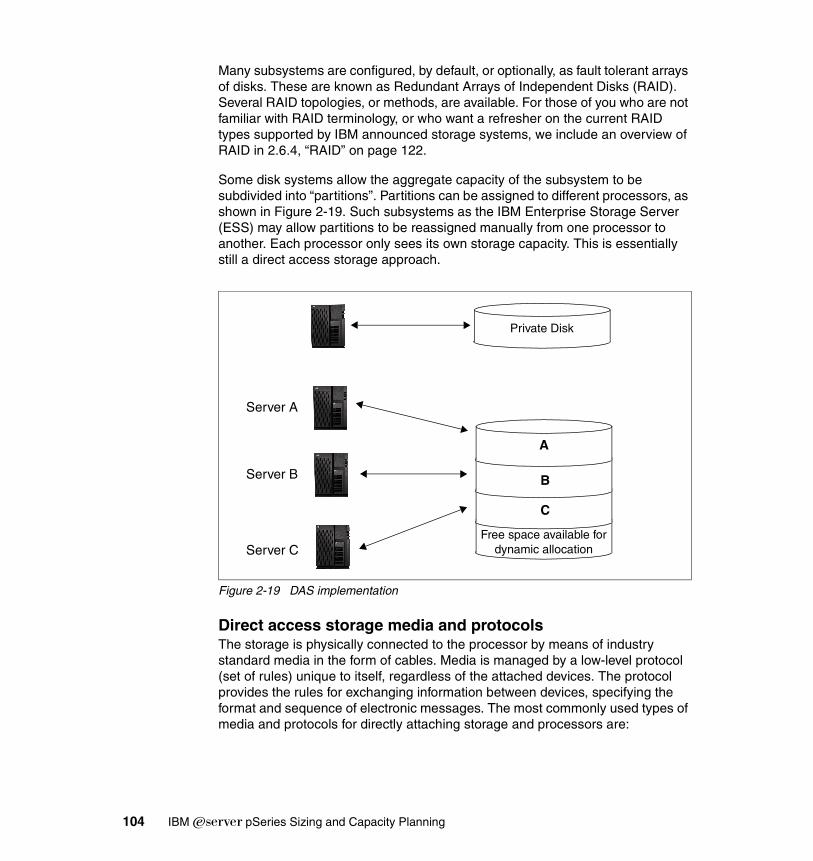
Many subsystems are configured, by default, or optionally, as fault tolerant arrays of disks. These are known as Redundant Arrays of Independent Disks (RAID). Several RAID topologies, or methods, are available. For those of you who are not familiar with RAID terminology, or who want a refresher on the current RAID types supported by IBM announced storage systems, we include an overview of RAID in 2.6.4, “RAID” on page 122.

Some disk systems allow the aggregate capacity of the subsystem to be subdivided into “partitions”. Partitions can be assigned to different processors, as shown in Figure 2-19. Such subsystems as the IBM Enterprise Storage Server (ESS) may allow partitions to be reassigned manually from one processor to another. Each processor only sees its own storage capacity. This is essentially still a direct access storage approach.

Figure 2-19 DAS implementation

Direct access storage media and protocolsThe storage is physically connected to the processor by means of industry standard media in the form of cables. Media is managed by a low-level protocol (set of rules) unique to itself, regardless of the attached devices. The protocol provides the rules for exchanging information between devices, specifying the format and sequence of electronic messages. The most commonly used types of media and protocols for directly attaching storage and processors are:

Free space available for dynamic allocation

A

B

C

Private Disk

Server A

Server B

Server C


� SCSI� Fibre Channel (FC)� Serial Storage Architecture (SSA)

SCSIThe parallel SCSI I/O bus, with its roots in the early 1980s, is the most commonly used interconnect media in open systems. An I/O bus is also known as a transport medium. As its name indicates, SCSI was designed for the PC and small computer environment. SCSI provides a high performance and reliable channel for data between servers and storage. Typical bandwidths range from 40 MB/s (Ultra SCSI), to 80 MB/s (Ultra2 SCSI), and 160 MB/s (Ultra160 SCSI). A parallel SCSI bus, using copper cable media, has a number of well-known limitations on scalability, connectivity, and distance (maximum of 25 meters), due to its use of parallel data transfers over eight or 16 data lines within the physical cable.

In addition to being a physical transport, SCSI is also a protocol. It specifies commands and controls for reading and writing blocks of data between the host and the attached disk devices. SCSI commands are issued by the host operating system in response to user requests for data. For instance, a SCSI I/O command may tell a disk device to return data from a specific location on the disk drive, or tell a tape library to mount a specific cartridge. The SCSI bus media is connected to the host server by a SCSI bus adapter (SBA). The SBA carries out much of the protocol mapping to disk with specialized firmware, optimizing performance of the data transfer. Some operating systems, such as Microsoft Windows NT®, treat all attached peripherals as SCSI devices and issue SCSI commands to deal with all I/O operations.

SCSI is a “block-level” protocol, called block I/O, since SCSI I/O commands define specific block addresses (sectors) on the surface of a particular disk drive. With SCSI protocols (block I/O), the physical disk volumes are visible to the servers that attach to them.

The distance limitations of parallel SCSI are addressed with the development of serial SCSI-3 protocols. These allow SCSI commands to be issued over different types of loop and network media, including Fibre Channel, SSA, and more recently IP Networks. Instead of being sent as a group of bits in parallel, on separate strands of wire within a cable, serial SCSI transports carry the signal as a stream of bits, one after the other, along a single strand of media.

Note: Throughout this book, we assume the use of SCSI protocols when we refer to directly attached storage.


Fibre ChannelFibre Channel is an open, technical standard for networking. It combines many of the data characteristics of an I/O bus, with the added benefits of the flexible connectivity and distance characteristics of a network. Fibre Channel uses serialized data transmission over either copper (for short distances up to 25 meters) or fiber optic media (for distances up to 10 kilometers). IBM devices only support the use of fiber optic media.

Storage devices may be directly attached to Fibre Channel enabled servers by means of point-to-point topology. They attach to a server’s host bus adapter (HBA).

Devices attached in this Fibre Channel point-to-point topology are, in effect, attached to a network comprising only two nodes. Because of its channel-like (bus) qualities, hosts and applications see storage devices as though they are locally attached storage.

Fibre Channel supports a number of low level storage protocols. When implemented with the SCSI command set, the low-level protocol is known as Fibre Channel Protocol (FCP). Bandwidth capability is 100 MB/s using full duplex with higher rates becoming available over time.

SSASSA is a powerful high performance serial interface. It was designed specifically for low-cost, high-performance connection to disk drives, optical drives, CD-ROMs, tape drives, printers, scanners, and other peripherals to personal computers, workstations, servers, and storage subsystems. It is the only serial interface that was designed from the outset to meet the requirements of a wide range of I/O devices.

SSA offers superior performance. Its fundamental building block is a single port capable of carrying on two 40 MB/sec. conversations at one time: one inbound and one outbound. An SSA connection consists of two ports capable of carrying on four simultaneous conversations, for a total bandwidth of 160 MB/sec.

SSA’s dual-port, full-duplex architecture allows peripherals to be connected in configurations with no single point of failure. Because multiple paths are inherent in the design, increased fault tolerance is far easier to implement. SSA provides hot plugging and automatic configuration when nodes are added or deleted. For

Note: The name host bus adapter is similar in name to the SCSI bus adapter. It clearly indicates that the Fibre Channel attachment is a “bus-like” attachment, using hardware assisted storage protocols. Like a SCSI bus, they communicate with the attached storage device by means of SCSI block I/O.


configuration flexibility, SSA nodes can be up to 25 meters apart using low-cost shielded twisted pair.

Direct access storage uses block I/OApplication programs and databases generate I/O requests, which culminate in data being read from, or written to, the physical storage device. I/O requests to directly attached storage, or to storage on a SAN, communicate in block I/Os. This is because the read and write I/O commands identify a specific device (disk drive or tape drive). In the case of disks, specific block (sector) locations on the disk are identified within the I/O request.

In the case of I/Os to disks using SCSI protocols, the application may use generalized file system services. These manage the organization of the data onto the storage device via the device driver software. In the UNIX world, this file-level I/O is called cooked I/O. However, many databases and certain specialized I/O processes generate record-oriented I/O direct to the disk via the device driver. UNIX fans call this raw I/O.

There is a fundamental characteristic of direct access storage (unlike some network storage devices). That is, regardless of whether the application uses cooked I/O or raw I/O (that is, file system or block access), all I/O operations to the device are translated to SCSI protocol blocks. That means they are formatted in the server by the database application, or by the operating system, into blocks which reflect the address and structure of the data on the physical disk device.

These blocks are moved on the I/O bus to the disk device, where they are mapped via a block table to the correct sector on the media (in mainframe parlance, this is called channel I/O). Block I/O is illustrated in Figure 2-20.

Figure 2-20 Direct access storage example

IP Network

ApplicationServer

Block I/O

SCSI Protocol

The application makes a file I/O request to a file system in the server, which initiates block I/O requests to the disk.

The application initiates raw block I/O requests to the disk.OR


Benefits of direct access storageIn summary, the benefits of direct access storage attachment are:

� Simplicity of connection

The cabling is either integrated in the cabinet with the server, or it is a simple point-to-point connection, often over short distances. Storage administrative skills required for installation are low.

� Low acquisition cost

SCSI bus cable costs are generally relatively low. Logistical planning and administrative overheads are kept to a minimum. Fibre Channel point-to-point connection costs are likely to be higher owing to the need for specialized HBAs and extended distances using fiber optic cables.

� High performance

The interconnection is designed for storage, and has a significant amount of hardware assistance to minimize software overheads. Direct access storage uses a storage protocol, such as SCSI block I/O, so performance is optimized for all types of applications.

� General purpose solution

Since the direct access storage solution is optimized for all types of storage processing, the investment in direct access storage can be applied to most applications. This gives good flexibility during the life of the acquisition.

Other direct access storage considerationsDirect access storage connections have several constraints:

� Limited scalability

The disk device can scale to a set maximum capacity. Bus connections normally and strictly limit the distance at which storage devices can be positioned from the server (maximum of 25 meters for parallel SCSI bus). They also limit the number of devices which can be attached to the bus (for example, a maximum of 15 on a parallel SCSI bus).

� Dedicated connectivity

This is often at a short distance. It prohibits the ability to share capacity resources with other servers. However, this limitation is mitigated in storage systems, such as the IBM TotalStorage Enterprise Storage Server (ESS). The ESS allows the connection of multiple servers, each attached to its own dedicated partition. SSA and FC point-to-point connections may also relieve distance limitations.


� Function

In many cases, low-cost disk systems attached to distributed clients and servers have limited function when compared to consolidated storage systems, which usually offer advanced capabilities such as RAID and enhanced copy services.

� Backup and data protection

Backup must be done to a server-attached tape device. This may lead to additional costs in acquiring multiple small tape devices. These may be acquired more for reasons of low cost rather than for quality and reliability associated with departmental or enterprise class devices. Individual users of direct access storage may apply inconsistent, or even non-existent, backup policies, leading to greater recovery costs in the event of errors or hardware failures.

� Total cost of ownership

Storage resources attached to individual servers are frequently and inefficiently used. Capacity that is available to one server is not available to other servers, unless the disk system allows attachment of multiple servers and partitioning. Storage administration costs are increased because the number of GBs an individual can manage in a distributed storage environment is substantially less than for consolidated storage such as NAS solutions.

2.6.2 Storage area networksA SAN is a specialized, dedicated high speed network. Servers and storage devices may attach to the SAN. It is sometimes called “the network behind the servers.” Like a LAN, a SAN allows any-to-any connections across the network, using interconnect elements such as routers, gateways, hubs, and switches. Fibre Channel is the de facto SAN networking architecture, although other network standards can be used.

Overview of Fibre Channel storage networksFibre Channel is an open, technical standard for networking. It incorporates the data delivery (OSI Transport layer) characteristics of an I/O bus with the flexible connectivity and distance characteristics of a network. One of the fundamental differences of SAN-attached storage, compared to NAS, is that SAN storage systems typically attach directly to the network by means of HBAs. NAS requires a front-end server as part of the appliance, which attaches to the LAN by means of a Network Interface Card (NIC).

A SAN eliminates the traditional dedicated connection between a server and direct access storage. Individual servers no longer own and manage the storage


devices. Restrictions to the amount of data that a server can access is also minimized. Instead, a SAN enables many heterogeneous servers to share a common storage “utility”. This utility may comprise many storage devices, including disk, tape, and optical storage. It may be located many kilometers from the servers which use it. Therefore, SAN-attached storage has the potential to be highly scalable relative to a typical NAS device.

Because of its channel, or bus-like, qualities, hosts and applications see storage devices attached to the SAN as though they are locally attached storage. With its network characteristics, it can support multiple protocols and a broad range of devices. It can also be managed as a network.

Fibre Channel is a multi-layered network, based on a series of American National Standards Institute (ANSI) standards. These standards define characteristics and functions for moving data across the network. Like other networks, information is sent in structured packets or frames, and data is serialized before transmission. Unlike other networks, the Fibre Channel architecture includes a significant amount of hardware processing. This is oriented to storage block I/O protocols, such as serial SCSI (known as FCP). Therefore, a SAN is capable of delivering high performance relative to an NAS device, which is optimized for network file I/O. The speed currently achieved is 100 MB/s full duplex, with 200 MB/s soon to be delivered.

Measured effective data rates of Fibre Channel have been demonstrated in the range of 60 to 80 MB/s over the 1 Gb/s implementation. This compares to less than 30 MB/s measured over Gigabit Ethernet. The packet size of Fibre Channel is 2,112 bytes (rather larger than some other network protocols). For instance, an IP packet is 1,518 bytes, although normally IP transfers are much smaller. For Fibre Channel, a maximum transfer unit sequence of up to 64 frames can be defined. It can allow transfers of up to 128 MB without incurring additional overhead due to processor interrupts. Today Fibre Channel is unsurpassed for efficiency and high performance in moving large amounts of data.

Transmission is defined in the Fibre Channel standards across three transport topologies:

� Point-to-point: This is a bi-directional, dedicated interconnection between two nodes. This delivers a topology similar to direct-attached storage, but with the added benefits of longer distance and reuse of the disks to a different server or even vendor of the future.

� Arbitrated loop (AL): This is a uni-directional ring topology, similar to a token-ring, supporting up to 126 interconnected nodes. Each node passes data to the next node in the loop, until the data reaches the target node. All nodes share the 100 MB/s bandwidth. Devices must arbitrate for access to the loop. FC-AL is suitable for small SAN configurations or SANlets.


� Switched fabric: This describes an intelligent switching infrastructure which delivers data from any source to any destination. Each node can use the full 100 MB/s bandwidth. Each logical connection receives dedicated bandwidth, so the overall bandwidth is multiplied by the number of connections. Complex fabrics must be managed by software that can exploit SAN management functions which are built into the fabric.

A mix of these three topologies can be implemented to meet specific needs.

SAN supports the following direct, high-speed transfers:

� Server-to-storage: This is similar to a direct-attached storage connection to a server. The SAN advantage, as with an NAS appliance, is that the same storage device may be accessed serially or concurrently by multiple servers.

� Server-to-server: This is high-speed communications between servers.

� Storage-to-storage: Outboard data movement means data can be moved with limited server intervention. Examples include a disk device moving data directly to a tape device, or remote device mirroring across the SAN.

Fibre Channel combines the characteristic strengths of traditional I/O channels with those of computer networks, in the following specifics:

� High performance for large data transfers by using storage transport protocols and extensive hardware assists

� Serial data transmission

� A physical interface with a low error rate definition

� Reliable transmission of data with the ability to guarantee or confirm error free delivery of the data

� Packaging data in packets (frames in Fibre Channel terminology)

� Flexibility in terms of the types of information which can be transported in frames (such as data, video, and audio)

� Use of existing device-oriented command sets, such as SCSI

� A vast expansion in the number of devices which can be addressed when compared to traditional I/O interfaces

This high degree of flexibility, availability, and scalability, over long distances make the Fibre Channel architecture attractive as the basis for new enterprise storage infrastructures. This attraction is also due to the broad acceptance of Fibre Channel standards by vendors throughout the IT industry.


Fibre Channel SANs using block I/OA SAN is similar to direct access storage to the extent that it is constructed from hardware and software storage interfaces. Fibre Channel uses serial SCSI-3 lower-level protocols which use block I/O access like a SCSI bus. Host-based file systems, database I/O management, or both are used, as with direct-attached storage. All I/Os across the SAN are block I/Os (see Figure 2-21). The conversion to blocks takes place in the client or server platform, before transmission of the I/O request over the network to the target storage device.

Figure 2-21 SAN example

Benefits of using SANsToday’s business environment creates many challenges for the enterprise IT planner. SANs can provide solutions to many of their operational problems. Among the benefits of implementing SANs are:

� Storage consolidation

By enabling storage capacity to be connected to servers at a greater distance, and by disconnecting storage resource management from individual hosts, a SAN enables disk storage capacity to be consolidated. The results can be lower overall costs through better utilization of the storage, lower management costs, increased flexibility, and increased control.

� Data sharing

The term data sharing is used somewhat loosely by users and some vendors. It is sometimes interpreted to mean the replication of files (File Transfer Protocol (FTP)-like). This enables two or more users or applications, possibly running on different host platforms, concurrently to use separate copies of the data. A SAN can minimize the creation of such duplicate copies of data by

IP Network

Block I/O

Fibre Channel Protocol

The application makes a file I/O request to a file system in the server, which initiates block I/O requests to a SAN-attached disk.

The application initiates raw block I/O requests to a SAN-attached disk.

OR

SAN

ServerApplication


enabling storage consolidation. Data duplication is also eased by using advanced copy services techniques found on enterprise class storage subsystems, such as remote mirroring and FlashCopy® on the ESS.

Data sharing can also be used to describe multiple users accessing a single copy of a file. This is the role for which an NAS appliance is optimized.

By enabling high-speed (100 MB/s) data sharing, the SAN solution may reduce traffic on the LAN and cut the cost of extra hardware required to store duplicate copies of data. It also enhances the ability to implement cross enterprise applications, such as e-business, which may be inhibited when multiple data copies are stored.

� Non-disruptive scalability for growth

A finite amount of disk storage can be connected physically to an individual server. With a SAN, new capacity can be added as required, without disrupting ongoing operations. SANs enable disk storage to be scaled independently of servers.

� Improved backup and recovery

With data doubling every year, what effect does this have on the backup window? Backup to tape and recovery operations can increase LAN overhead.

– Tape pooling: SANs allow for greater connectivity of tape drives and tape libraries, especially at greater distances. Tape pooling is the ability for more than one server to logically share tape drives within an automated library.

– LAN-free and server-free data movement: Backup using the LAN may cause high traffic volumes, which may be disruptive to normal application access to the network. SANs can minimize the movement of backup and recovery data across the LAN. The IBM Tivoli software solution for LAN-free and server-free backup offers the capability for clients to move data directly to tape using the SAN.

� High performance

Many applications benefit from the more efficient transport mechanism of Fibre Channel. Most of the elements of FCP are implemented in hardware to increase performance and efficiency.

� High availability server clustering

Reliable and continuous access to information is an essential prerequisite in any business. Server and software vendors developed high availability solutions based on clusters of servers. SCSI cabling tends to limit clusters to no more than two servers. A Fibre Channel SAN allows clusters to scale to 4, 8, 16, and even to 100 or more servers, as required, to provide large shared data configurations.


� Data integrity

In Fibre Channel SANs, the class of service setting, such as Class 2, guarantees delivery of frames. Sequence checking and acknowledgement is handled in the hardware, without incurring additional overhead. This compares to IP networks, where frames may be dropped in the event of network congestion, causing problems for data-intensive applications.

� Disaster recovery

Sophisticated functions, such as Peer-to-Peer Remote Copy (PPRC) services, address the need for secure and rapid recovery of data in the event of a disaster. A SAN implementation allows multiple open servers to benefit from this type of disaster protection. The servers may be located at campus and metropolitan distances (up to between 10 km and 20 km) from the disk array which holds the primary copy of the data. The secondary site, holding the mirror image of the data, may be located up to a further 100 km from the primary site.

� Selection of “best-of-breed” storage

A SAN enables storage purchase decisions to be made independently of the server. Buyers are free to choose the best-of-breed solution to meet their performance, function, and cost needs. Large capacity external disk arrays may provide an extensive selection of advanced functions.

Client/server backup solutions often include attachment of low capacity tape drives to individual servers. This introduces a significant administrative overhead since users often have to control the backup and recovery processes manually. A SAN allows the alternative strategy of sharing fewer, highly reliable, centralized tape solutions, (such as IBM Magstar® and Linear Tape Open solutions), between multiple users and departments.

� Ease of data migration

When using a SAN, data can be moved non-disruptively from one storage subsystem to another, bypassing the server. Eliminating the use of server cycles may greatly ease the migration of data from old devices when introducing new technology.

� Reduced TCO

Consolidation of storage in a SAN can reduce wasteful fragmentation of storage attached to multiple servers. A single, consistent data and storage resource management solution can be implemented. This can reduce costs of software and human resources for storage management compared to distributed direct-attached storage systems.


� Storage resources match e-business enterprise needs

By eliminating islands of information, and introducing an integrated storage infrastructure, SAN solutions can be designed to match the strategic needs of today’s e-business.

Other SAN considerationsThere are pros and cons to most decisions. You must consider the following issues, as well as others, when making a SAN investment.

� Costs

SAN entails installation of a new, dedicated Fibre Channel network infrastructure. The cost of the fabric components, such as Fibre Channel HBAs, hubs, and switches, is an important consideration. Today these costs are significantly higher than the equivalent Ethernet connections and fabric components. An additional cost is the IT personnel, who may demand higher salaries due to their specialized Fibre Channel knowledge.

� Inter-operability

Unlike Ethernet LANs, which have been implemented for more than fifteen years, Fibre Channel is still relatively early in its development cycle. Several important industry standards are in place, while others have yet to be agreed upon. This has implications for ease of interoperability between different vendors’ hardware and software. This may cause added complexity to the implementation of multivendor, heterogeneous SANs. However, this issue is gradually going away over time owing to industry-wide efforts in interoperability testing and cooperation on development of standards.

� Storage wide area networks (SWAN)

Today Fibre Channel protocol SANs are mostly restricted in scope to the size of a LAN, due to the limited distances (10 kilometers) supported by the Fibre Channel architecture. This has implications when considering the interconnection of multiple SANs into a SWAN. Such interconnections require protocol conversions to other transport technologies, such as asynchronous transfer mode (ATM) or TCP/IP, and the costs are high. Future implementations of FCP are expected to enable SANs to network across wider domains than a LAN. It is likely to be years before this is available.

� Skills

Due to Fibre Channel’s introduction and explosive growth (started to take off only in 1998), people with the necessary skills are still relatively scarce. Employment of new staff with appropriate experience may be difficult or costly. It is often necessary to invest in extensive education of your own staff or use external services (such as IBM Global Services), which have developed the necessary skills and have wide experience with SAN implementations.


� Lack of reach

To extend access to the SAN requires installation of a Fibre Channel connect for each server. This configuration increases TCO.

SAN sizing considerationsThese are some considerations that you must make for your SAN sizing:

� The storage elements that include your tape drives and libraries, disk storage, optical storage, and intelligent storage servers (defined as storage subsystem, each having a storage control processor, cache storage, and cache management algorithms): You need to identify how many of this storage elements you will place in your SAN environment.

� The SAN fabric is built from interconnecting elements such as FC hubs, FC switches, routers, bridges, and gateways. These components transfer Fibre Channel packets from server to storage, server to server, and storage to storage, depending on the configurations supported and the functions used. After you identify how many storage elements you want put in your SAN environment, your IBM representative must assist you with the latest FC switches, routers, bridges, and gateways that you will need. Remember there’s no such thing as “one size fits all”.

� The server that wants to be connected to the fabric: Applications want to take advantage of the SAN’s benefit. Identify how many servers you need to place in SAN environment. This help you determine how many Fibre Channel cards you need and the kind of SAN fabric you will use.

� In software, there are two kinds of software management applications:

– Fabric management applications used to configure, manage, and control the SAN fabric

– Applications that exploit the SAN functions to bring business benefits such as improved backup or recovery and remote mirroring

� You need to plan for your future growth.

After you identify how many storage elements (SAN fabric, server, and software) you need, you can size your SAN environment.

2.6.3 Network-attached storageStorage systems that optimize the concept of file sharing across the network use NAS. NAS solutions use the mature Ethernet IP network technology of the LAN. Data is sent to and from NAS devices over the LAN using TCP/IP.

By making storage systems LAN addressable, the storage is freed from its direct attachment to a specific server. Any-to-any connectivity is facilitated using the


LAN fabric. In principle, any user running any operating system can access files on the remote storage device. This is done by means of a common network access protocol, for example, Network File System (NFS) for UNIX servers and CIFS for Windows servers. In addition, a task, such as backup to tape, can be performed across the LAN using such software as IBM Tivoli Storage Manager (TSM). This enables the sharing of expensive hardware resources (for example, automated tape libraries) between multiple servers.

A storage device cannot just attach to a LAN. It needs intelligence to manage the transfer and the organization of data on the device. The intelligence is provided by a dedicated server to which the common storage is attached. It is important to understand this concept. NAS comprises a server, an operating system, and storage which is shared across the network by many other servers and clients. A NAS is a specialized server or appliance, rather than a network infrastructure, and shared storage is attached to the NAS server.

The NAS system “exports” its file system to clients, which access the NAS storage resources over the LAN.

File serversNAS solutions have evolved over time, beginning in the mid 1990s. Early NAS implementations used a standard UNIX or Windows NT server with NFS or CIFS software to operate as a remote file server. Clients and other application servers access the files stored on the remote file server as though the files are located on their local disks. The location of the file is transparent to the user. Several hundred users could work on information stored on the file server, each one unaware that the data is located on another system.

The file server has to manage I/O requests accurately, queuing as necessary, fulfilling the request, and returning the information to the correct client. The NAS server handles all aspects of security and lock management. If one user has the file open for updating, no one else can update the file until it is released. The file server keeps track of connected clients by means of their network IDs, addresses, and so on.

Network appliancesLater developments use application specific, specialized thin server configurations with customized operating systems. These operating systems usually comprise a stripped down UNIX kernel, reduced Linux operating system, or a specialized Windows 2000 kernel, as with the IBM NAS appliances described in this book. In these reduced operating systems, many of the server operating system functions are not supported. It is likely that many lines of operating system code were removed. The objective is to improve performance and reduce costs by eliminating unnecessary functions normally found in the


standard hardware and software. Some NAS implementations also employ specialized data mover engines and separate interface processors in efforts to further boost performance.

These specialized file servers with reduced operating system are typically known as appliances, describing the concept of an application-specific system. The term appliance, taken from household electrical devices, is the idea of a specialized plug-and-play, application-specific tool, such as a coffee maker or a toaster. Indeed, specialized NAS appliances, such as the IBM TotalStorage NAS solutions, come with preconfigured software and hardware and without a monitor or keyboard for user access. This is commonly termed a headless system. A storage administrator can access the device and manage the disk resources from a remote console.

A typical characteristic of an NAS appliance is its ability to be installed rapidly, with minimal time and effort to configure the system, and to integrate it into the network. This plug-and-play approach makes NAS appliances especially attractive when lack of time and skills are elements in the decision process.

A NAS appliance is an easy-to-use device. It is designed for a specific function, such as serving files to be shared among multiple servers, and performs this task well. It is important to recognize this when selecting an NAS solution since it is not a general purpose server. It should not be used (due to its reduced operating system, probably cannot be used) for general purpose server tasks. But it provides a good solution for appropriately selected shared storage applications.

The IBM 3466 Network Storage Manager (NSM) is an integrated appliance that provides backup, archive, storage management, and disaster recovery of data stored in a network computing environment. The NSM integrates Tivoli Storage Manager server functions with a rack mounted pSeries, SSA disk storage, network communications. It links to automated tape libraries. NSM manages clients’ data, providing easily installed, centrally administered storage management services in a distributed network environment.

The IBM 3466 NSM is an example of a specialized, plug-and-play IBM network-attached appliance. It requires limited administrator skills to implement a comprehensive data backup and protection solution. Since the focus of this book is on recently announced NAS disk storage, we do not include further details about the IBM 3466. For more information about this powerful backup/restore product, see A Practical Guide to Network Storage Manager, SG24-2242.

NAS appliances using file I/OA key difference in an NAS appliance, compared to direct access storage or other network storage solutions such as SAN or iSCSI, is that all client I/O operations to the NAS use file-level I/O protocols. File I/O is a high-level type of


request that, in essence, specifies only the file to be accessed. It does not directly address the storage device. This is done later by other operating system functions in the remote NAS appliance.

A file I/O specifies the file. It also indicates an offset into the file. For instance, the I/O may specify “Go to byte ‘1000’ in the file (as though the file were a set of contiguous bytes), and read the next 256 bytes beginning at that position”. Unlike block I/O, there is no awareness of a disk volume or disk sectors in a file I/O request. Inside the NAS appliance, the operating system keeps track of where files are located on disk. The NAS operating system issues a block I/O request to the disks to fulfill the client file I/O read and write requests it receives.

In summary, network access methods, such as NFS and CIFS, can only handle file I/O requests to the remote file system. This is located in the operating system of the NAS device. I/O requests are packaged by the initiator into TCP/IP to move across the IP network. The remote NAS file system converts the request to block I/O and reads or writes the data to the NAS disk storage. To return data to the requesting client application, the NAS appliance software repackages the data in TCP/IP to move it back across the network. Figure 2-22 illustrates this.

Figure 2-22 NAS example

NAS benefitsNAS offers a number of benefits, which address some of the limitations of directly attached storage devices, and overcome some of the complexities associated with SANs. NAS benefits include:

� Resource pooling

A NAS appliance enables disk storage capacity to be consolidated and pooled on a shared network resource, at great distance from the clients and

IP Network

File I/O

Internet Protocol (IP)

ApplicationServer

NAS Appliance

The application server directs the file I/O request over the LAN to the remote

file system in the NAS appliance.

The file system in the NAS appliance initiates a block I/O to

the NAS integrated disk.


servers which will share it. Therefore an NAS appliance can be configured as one or more file systems, each residing on specified disk volumes. All users accessing the same file system are assigned space within it on demand. This contrasts with individual DAS storage, when some users may have too little storage, and others may have too much.

Consolidation of files onto a centralized NAS device can minimize the need to have multiple copies of files spread among distributed clients. Thus overall hardware costs can be reduced.

NAS pooling can reduce the need to physically reassign capacity among users. The results can be lower overall costs through better utilization of the storage, lower management costs, increased flexibility, and increased control.

� Exploits existing IP network infrastructure

Because NAS uses the existing LAN infrastructure, there are minimal costs of implementation. Staff with existing skills in IP networks can perform the installation.

� Simple to implement

Because NAS devices attach to mature, standard LAN infrastructures, and have standard LAN addresses, they are extremely easy to install, operate, and administer. This plug-and-play operation results in low risk, ease of use, and fewer operator errors, so it contributes to a lower cost of ownership.

� Enhanced choice

The storage decision is separated from the server decision. This enables buyers more choice in selecting equipment to meet their business needs.

� Connectivity

LAN implementation allows any-to-any connectivity across the network. NAS appliances may allow for concurrent attachment to multiple networks to support many users.

� Scalability

NAS appliances can scale in capacity and performance within the allowed configuration limits of the individual appliance. However, this may be restricted by such considerations as LAN bandwidth constraints and the need to avoid restricting other LAN traffic.

� Heterogeneous file sharing

A major benefit of NAS is support of multiple client file systems. Most organizations support mixed platform environments, such as UNIX and Windows. In a distributed server-based environment, a dedicated server is required for each file system protocol. If one department is using Windows-based office applications while another is using UNIX-based


computer-aided design, two independent servers with their own directly attached storage are required and must be supported by the IT organization.

Remote file sharing is one of the basic functions of any NAS appliance. Most NAS systems support multiple operating system environments. Multiple client systems can have access to the same file. Access control is serialized by NFS or CIFS. Heterogeneous file sharing is enabled by the provision of translation facilities between NFS and CIFS. For users, this means flexibility and standardization of file services. It can also mean cost savings in staffing, training, and deployment.

� Improved manageability

By providing consolidated storage, which supports multiple application systems, storage management is centralized. This enables a storage administrator to manage more capacity on an NAS appliance than is possible for distributed storage directly attached to many independent servers.

� Reduced TCO

Because of its use of existing LAN network infrastructures, and of network administration skills already employed in many organizations (such as Tivoli NetView® management), NAS costs may be substantially lower than for directly-attached or SAN-attached storage.

Other NAS considerationsOn the converse side of the storage network decision, you must consider the following factors regarding NAS solutions:

� Proliferation of NAS devices

Pooling of NAS resources can only occur within the capacity of the individual NAS appliance. As a result, to scale for capacity and performance, there is a tendency to grow the number of individual NAS appliances over time, which can increase hardware and management costs.

� Software overhead impacts performance

TCP/IP is designed to bring data integrity to Ethernet-based networks by guaranteeing data movement from one place to another. The trade-off for reliability is a software-intensive network design which requires significant processing overheads, which can consume more than 50% of available processor cycles when handling Ethernet connections. This is not normally an issue for applications, such as Web browsing, but it is a drawback for performance-intensive storage applications.

� Consumption of LAN bandwidth

Ethernet LANs are tuned to favor short burst transmissions for rapid response to messaging requests, rather than large continuous data transmissions. Significant overhead can be imposed to move large blocks of data over the


LAN. This is due to the small packet size used by messaging protocols. Because of the small packet size, network congestion may lead to reduced or variable performance, so the LAN must have plenty of spare capacity to support NAS implementations.

� Data integrity

Ethernet protocols are designed for messaging applications, so data integrity is not of the highest priority. Data packets may be dropped without warning in a busy network, and have to be resent. It is up to the receiver to detect that a data packet has not arrived, and to request that it be resent, so this can cause additional network traffic.

� Impact of backup/restore applications

A potential downside of NAS is the consumption of substantial amounts of LAN bandwidth during backup and restore operations, which may impact other user applications. NAS devices may not suit applications that require very high bandwidth.

� Suitability for database

Given that their design is for file I/O transactions, NAS appliances are not optimized for the I/O demands of some database applications. They do not allow the database programmer to exploit “raw” block I/O for high performance. As a result, typical databases, such as Oracle or DB2® Universal Database™ (UDB), do not perform as well on NAS devices as they would on DAS, SAN, or iSCSI. However, some clients may choose to use NAS for database applications with file I/O because of their other advantages, including lower cost. It is important to that, in some cases, the database vendor may prohibit use of NAS appliances with their software. For instance, Microsoft does not support the use of NAS devices with Microsoft Exchange. In such cases, other storage solutions must be found.

2.6.4 RAIDRAID is an architecture designed to improve data availability by using arrays of disks in conjunction with data striping methodologies. The idea of an array is a collection of disks the system sees as a single device. There are different levels of RAID. RAID levels 1 through 5 were defined in the original Berkeley RAID paper. Subsequently, RAID levels 0 and 6 were developed.

RAID levelsFigure 2-23 through Figure 2-26 on page 126 graphically explain RAID levels 0, 1, 3, and 5, the most commonly implemented RAID architectures. Figure 2-28 on page 129 gives a similar explanation for RAID level 6. For convenience, RAID level 0 through RAID level 6 are referred to as RAID 0 through RAID 6.


Parity is defined as redundant information about user data, which allows it to be regenerated in the event of a disk failure. In the following illustrations, data can mean a byte or block, not necessarily an entire file.

RAID 0Data striping with no parity is not a true RAID architecture because there is no data redundancy. RAID 0 stripes data sequentially across multiple disks to allow parallel read or write operations. This can result in high, effective data transfer rates. All RAID 0 implementations spread the data and workload across the disks in the array, which often gives higher throughput than non-striped disks. However, RAID 0 does not provide redundancy with the performance boost. As shown in Figure 2-23, in the event of a single disk failure, the data residing on the disk cannot be regenerated. Because of data striping, all data becomes unavailable.

Figure 2-23 RAID 0

RAID 1The RAID 1 implementation in Figure 2-24 employs data mirroring to achieve redundancy. Two copies of the data are created and maintained on separate

Note: Never use RAID level 0 for critical applications that require high data availability. Consider it only for applications that can benefit from the performance capabilities of this level.

RAID 0 – Striping (4 Stripes Example)

Data n(1/4)

Data 2(1/4)Data 1(1/4)

Data n(2/4)

Data 2(2/4)Data 1(2/4)

Data n(3/4)

Data 2(3/4)Data 1(3/4)

Data n(4/4)

Data 2(4/4)Data 1(4/4)

Data 1

Data 2

:

Data n


Data n(1/4)

Data 2(1/4)Data 1(1/4)

Data n(2/4)

Data 2(2/4)Data 1(2/4)

Data n(3/4)

Data 2(3/4)Data 1(3/4)

Data n(4/4)

Data 2(4/4)Data 1(4/4)

Data 1

Data 2

:

Data n


Data n(1/4)

Data 2(1/4)Data 1(1/4)

Data n(1/4)Data n(1/4)

Data 2(1/4)Data 2(1/4)Data 1(1/4)Data 1(1/4)

Data n(2/4)

Data 2(2/4)Data 1(2/4)



Data n(3/4)

Data 2(3/4)Data 1(3/4)



Data n(4/4)

Data 2(4/4)Data 1(4/4)



Data 1

Data 2

:

Data n


disks, each containing a mirror image of the other. RAID 1 provides an opportunity to improve performance for reads, because read requests are directed to the mirrored copy if the primary copy is busy.

RAID 1 is the most expensive of the array implementations because the data is duplicated. However, it provides the best data availability from a disk failure standpoint, because it uses the fewest disks in its array configuration. The fewer the disks there are in an array, the lower the probability is of multiple disk failures. In the event of a disk failure, RAID 1 provides the highest performance, because the system can switch automatically to the mirrored disk without impacting performance and needing to rebuild lost data.

Figure 2-24 RAID 1

RAID 2RAID 2 supports parallel access and data striping with hamming code. At a conceptual level, RAID 2 and RAID 3 are similar. Both RAID 2 and RAID 3 distribute data across several disks with striping at the bit, byte, or multibyte level. The data is written or retrieved in one parallel movement of all of the access arms.

RAID 2, however, uses an encoding technique called the hamming error correction code to provide error detection and correction. This encoding technique requires multiple disks for the error detection and correction information, making the RAID 2 parity implementation more complex and more expensive for general use than the RAID 3 design. Therefore, RAID 2 is of little interest in a commercial environment.

Note: Consider RAID 1 when cost is not a factor for applications that require high data availability and high performance.

RAID 1 – Mirroring

Data n

Data 2Data 1

Data n

Data 2Data 1

Data 1

Data 2

:

Data nData n

Data 2Data 1

Data n

Data 2Data 1


RAID 3RAID 3 supports parallel access and data striping with parity. Unlike RAID 2, RAID 3 uses a single dedicated disk to store parity information. Like RAID 2, RAID 3 stripes or distributes data sequentially across several disks. The data is written or retrieved in one parallel movement of all of the access arms.

Figure 2-25 shows an array of four disks. Three of the disks are used to store data, and the fourth disk is used to store parity for the three data disks. If one of the data disks fails, the parity disk can be used, along with the remaining data disks, to regenerate the data. If the parity disk fails, access to data is not affected. Because of the single parallel movement of all access arms, only one I/O can be active in the array at any one time. Because data is striped sequentially across the disks, the parallel arm movement yields excellent transfer rates for large blocks of sequential data. However, it renders RAID 3 impractical for transaction processing or other high throughput applications needing random access to data. When random processing takes place, the parity disk becomes a bottleneck for write operations.

Figure 2-25 RAID 3

Note: Use RAID 3 for applications that process mostly large blocks of data or require access to large sequential data files.

RAID 3 – Striping with Dedicated Parity

Data n(1/3)

Data 2(1/3)Data 1(1/3)

Data n(2/3)

Data 2(2/3)Data 1(2/3)

Data n(3/3)

Data 2(3/3)Data 1(3/3)

Parity n

Parity 2Parity 1

Data 1

Data 2

:

Data n

RAID 3 – Striping with Dedicated Parity

Data n(1/3)

Data 2(1/3)Data 1(1/3)



Data n(2/3)

Data 2(2/3)Data 1(2/3)



Data n(3/3)

Data 2(3/3)Data 1(3/3)



Parity n

Parity 2Parity 1

Data 1

Data 2

:

Data n


RAID 4RAID 4 supports independent access and data striping with dedicated parity. Like RAID 2 and RAID 3, RAID 4, and RAID 5 stripe data across several disks, but the striping increment is a block or record. There is only one parity disk in the RAID 4 design. In all other aspects RAID 4 is identical to RAID 5.

Because the parity disk is involved in every write operation, it can become a bottleneck for transaction throughput. Therefore, RAID 4 is not considered viable for commercial applications.

RAID 5RAID 5 supports independent access and data striping with distributed parity. It does not have a dedicated parity disk, but interleaves data and parity on all disks. In RAID 5, the access arms can move independently of one another as shown in Figure 2-26. This enables multiple concurrent accesses to the array devices. It satisfies multiple concurrent I/O requests and provides higher transaction throughput. RAID 5 is best suited for random access data in small blocks.

Figure 2-26 RAID 5

An important difference between RAID 3 and RAID 5 is that, in RAID 3, every transfer involves all of the disks. In RAID 5, most transfers involve only one data disk. This allows operations in parallel and gives higher throughput for transaction processing. In RAID 3, the segment size is one sector, and the unit of

RAID 5 – Striping with Distributed Parity

Data 6Parity(1-3)

Data 1

Data 2

Data 3

Data 4

Data 5

Data 6

Data 7

Data 8

Data 9

Data 4Data 1

Data 5Data 2

Parity(4-6)Data 3

Data 7

Parity(7-9)

Data 8

Data 9

RAID 5 – Striping with Distributed Parity

Data 6Parity(1-3)

Data 1

Data 2

Data 3

Data 4

Data 5

Data 6

Data 7

Data 8

Data 9

Data 4Data 1

Data 5Data 2

Parity(4-6)Data 3

Data 7

Parity(7-9)

Data 8

Data 9


transfer is one sector for each data disk. In RAID 5, the segment size is larger, and most transfers involve only one data disk, allowing operations in parallel and giving higher throughput.

A write penalty is associated with RAID 5. Every write I/O results in four actual I/O operations, two to read the old data and parity, and two to write the new data and parity.

Reducing the write penaltyA way to reduce the RAID 5 write penalty is to use cache. This allows increased performance by temporarily storing data in anticipation of I/O requests to disk. By retaining accessed data in cache, read requests for the same information can be quickly satisfied from cache without additional I/O operations to disk. This can reduce disk I/O because of the locality of reference in access patterns.

Cache can be used to bundle write requests until a large block of contiguous data can be written to disk in a single I/O operation. During write operations, data is first written to cache, allowing a transaction to complete sooner than the actual write operation to disk. By allowing the application to proceed in parallel with actual physical I/O operations, cache can reduce the delay associated with reading or writing data and improve RAID 5 performance.

Nonvolatile storage (NVS) keeps data stored in cache from being lost when a power outage occurs. NVS is the cache that switches to battery power during an outage. Under normal circumstances, NVS functions in much the same manner as regular cache. As soon as a write request is completed to NVS, the application can proceed without further delay. However, if an outage occurs, the updated data is still safely stored in NVS until that data can be written to the disk.

NVS is in all ESS models and IBM TotalStorage Fibre Array Storage Technology (FAStT), except the low-end FAStT 200. Figure 2-27 shows a two-node system in normal operation. The ensemble consists of subsystem A (runs with SMP 1 and NVS 2) and subsystem B (runs with SMP 2 and NVS 1).

The right half of Figure 2-27 shows the failover of node 1 and node 2. The surviving node assumes ownership of all host adapter (initially ownership is shared), the nonvolatile storage on the node, and all physical devices in the system. The surviving node then restores redundancy by destaging (writing modified user data from cache to the disk arrays) all modified data in its read cache and data in the local nonvolatile storage belonging to the failed node. The node then allows the host adapters to recognize that all virtual disks are owned by the surviving node. Then the node resumes operation using the local NVS as its NVS.


Figure 2-27 IBM TotalStorage Enterprise Storage System

RAID 6Independent access, data striping with double distributed parity, which was not among the original Berkeley RAID levels, adds a second, independent parity block to RAID 5. Figure 2-28 shows an example of RAID 6 with an array of six disks. Four disks are used for data, and two disks are used for parity, with data and parity rotating and interleaving within the array.

With two independent parity schemes, each using a different algorithm, data availability is extremely good. It is uninterrupted even when two disk failures occur at the same time. However, more disk space is required for parity. There is an even greater write penalty than with RAID 5. For this reason, the write performance of RAID 6 is extremely low. The lower performance and the complexity of implementation have made RAID 6 impractical for most applications.

Note: Consider RAID 5 for environments that require high data availability and with applications that process relatively short data records or a mixture of large sequential records and short random blocks.


Figure 2-28 RAID 6

RAID 10RAID 10 consists of a set of disks for user data plus their mirrored disks counterparts. There is no parity disk to rebuild a failed disk. In case one disk becomes unusable, then the mirror copy is used to access the data and to build the spare (also known as RAID 0+1).

Because it is a combination of RAID 0 (striping) and RAID 1 (mirroring). The striping optimizes the performance by striping volumes across several disk drives. Figure 2-29 shows, for example, in the ESS Model 800 implementation, three or four disk drive modules (DDMs). RAID 1 is the protection against a disk failure by having a mirrored copy of each disk. By combining the two, RAID 10 provides data protection with I/O performance.

RAID 6 – Striping with Double Distributed Parity

Data 1

Data 2

Data 3

Data 4

Data 5

Data 6

Data 7

Data 8

Data 9

Data 10

Data 11

Data 12

Data 5Data 1

Data 9

Data 6Data 2

Data 10

Data 7Data 3

Parity(9-12)

Data 4

Parity(9-12)Parity(5-8)

Data 4

Parity(9-12)Parity(5-8)

Data 11

Parity(5-8)Parity(1-4)Parity(5-8)Parity(1-4)

Data 12Data 8

Parity(1-4)

Data 11


Figure 2-29 RAID 10

It is possible to combine RAID 10 and RAID 5 configured within the same loop, as illustrated in Figure 2-30. There are several ways in which a loop can be configured when mixing RAID 5 and RAID 10 ranks in it. If you configure RAID 5 and RAID 10 ranks on the same loop, it is important to follow some guidelines to balance the capacity between the clusters.

Data

1

Data

2

Data

3

Spare

S

Data

1

Data

2

Data

3

Data

4

Data

11

Data

21

Data

31

Spare

S

Data

11

Data

21

Data

31

Data

41

Eight-pack 2

Eight-pack 1

Eight-pack Pair 1

Data

1

Data

2

Data

3

Data

1

Data

2

Data

3

Data

4

Data

11

Data

21

Data

31

Data

11

Data

21

Data

31

Data

41

Eight-pack 4

Eight-pack 3

Eight-pack Pair 2

Data

4

Data

41

RAID 10 configurations

� First RAID 10 rank configured in the loop is 3+3+2S.

� Additional RAID 10 ranks configured in the loop are 4+4.

� For a loop with an intermixed capacity, the ESS assigns two spares for each capacity. This means that there is one 3+3+2S array per capacity.


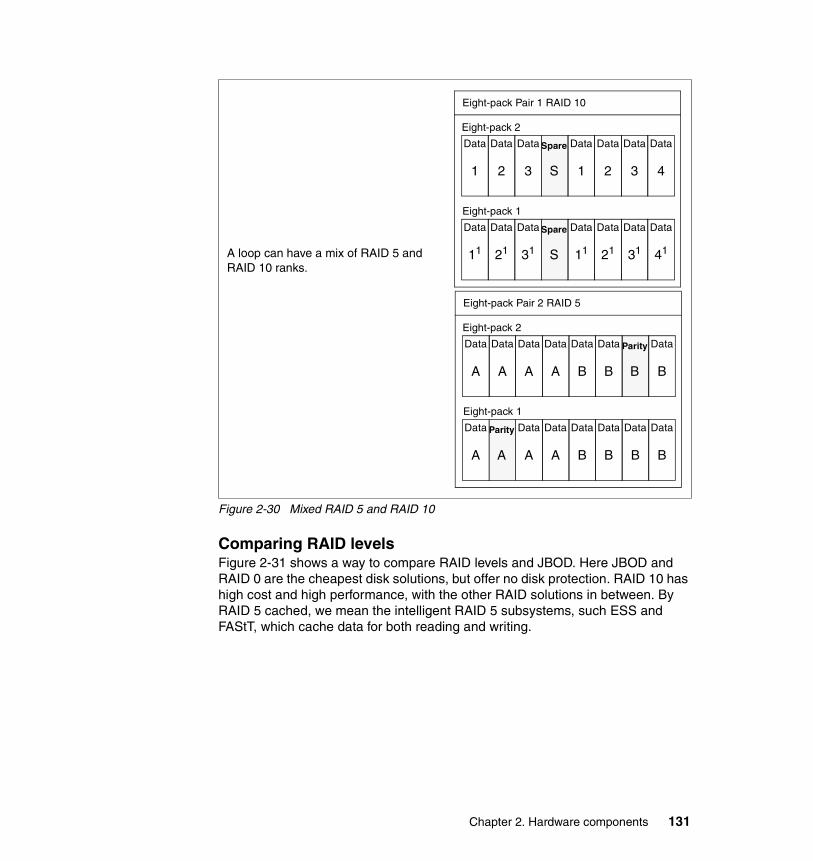
Figure 2-30 Mixed RAID 5 and RAID 10

Comparing RAID levelsFigure 2-31 shows a way to compare RAID levels and JBOD. Here JBOD and RAID 0 are the cheapest disk solutions, but offer no disk protection. RAID 10 has high cost and high performance, with the other RAID solutions in between. By RAID 5 cached, we mean the intelligent RAID 5 subsystems, such ESS and FAStT, which cache data for both reading and writing.

Data

1

Data

2

Data

3

Spare

S

Data

1

Data

2

Data

3

Data

4

Data

11

Data

21

Data

31

Spare

S

Data

11

Data

21

Data

31

Data

41

Eight-pack 2

Eight-pack 1

Eight-pack Pair 1 RAID 10

Data

A

Data

A

Data

A

Parity

B

Data

B

Data

B

Data

B

Data

A

Data

A

Data

A

Parity

A

Data

B

Data

B

Data

B

Data

B

Eight-pack 2

Eight-pack 1

Eight-pack Pair 2 RAID 5

Data

A

A loop can have a mix of RAID 5 and RAID 10 ranks.


Figure 2-31 Cost, performance, and availability

Table 2-1 compares the RAID levels.

Table 2-1 Comparison of RAID levels

Low Cost

High Cost

HighlyAvailableHigh

PerformanceRAID5simple

JBOD

RAID 10 (0+1) stripe+mirror

RAID 0 stripe

RAID 1mirror

RAID 5cached RAID 5

simple

RAID 0 RAID 1 RAID 3 RAID 5 RAID 10

Method used Disk striping

Disk level mirroring

Parallel transfer disks with parity

Independent data access

Mirror

Disks required n 2n n+1 n+1 2n

Data protection

None Very high High High Very high

Data rate Very high For read: 2 X single disk; for write, similar to single disk

Similar to single disk

Similar to single disk

For read from 2X single disk; for write, similar to single disk

Performance High High for read-intensive; medium for write-intensive

Medium Medium (possible write penalty in write-intensive environment

High

Cost Low High (up to twice RAID 0 costs)

Medium Medium High


2.6.5 IBM TotalStorage Enterprise Storage ServerThe IBM TotalStorage ESS is the most powerful disk storage server, developed by IBM using IBM Seascape® architecture. The ESS provides unmatchable functions for the entire server family of e-business servers and for the non-IBM (that is, Intel-based and UNIX-based) families of servers.

Across all of these environments, the ESS features unique capabilities that allow it to meet the most demanding requirements of performance, capacity, and data availability that the computing business may require. The Seascape architecture is the key to the development of IBM storage products. Seascape allows IBM to take the best of the technologies developed by the many IBM laboratories and integrate them, producing flexible and upgradable storage solutions. This Seascape architecture design has allowed the ESS to evolve from the initial E models to the succeeding F models, and to the recently announced 800 models. Each feature new, more powerful hardware and functional enhancements. They are always integrated under the same successful architecture with which the ESS was originally conceived.

The ESS concurrently supports diverse host systems over diverse attachment protocols. You can allocate data storage among the attached host systems with the ESS Specialist, a Web-based interface. The ESS provides integrated caching and support for the attached DDMs. The DDMs are attached through a SSA interface. Disk storage on an ESS is available in modules that contain eight DDMs called eight packs.

The ESS provides the major following features:

� Hardware fault-tolerant, including dual write caches

� Support of an intermix of types of RAID

� Support of non-RAID disk groups

� Fast RISC processors

� Fast disk drives with speeds of 10,000 and 15,000 rpm

� Disk capacity that you can assign and reassign among attached host systems

� Instant copy solutions with FlashCopy

� Disaster recovery solutions with PPRC

� Concurrent repairs (“hot swap”)

� Concurrent hardware upgrades

� Concurrent software/microcode changes

Note: ESS Model 800 does not support non-RAID disk groups.


� Auto Call Home for service and scheduled proactive Call Home to confirm status

� Remote problem analysis and diagnostics

� Multiple event client notification facilities: Simple Network Management Protocol (SNMP), e-mail, pager

� Flexible Fibre Channel SAN support including directors, hubs, and switches

� SAN logical unit number (LUN) masking (security) support standard

� Support for CIFS, FTP, Hypertext Transfer Protocol (HTTP), NetWare, and NFS file-I/O (NAS) protocols

� Support for iSCSI via a CISCO Storage Router

� Host multipathing software (subsystem device driver (SDD) for load balancing and failover)

� Standard three-year hardware and software feature warranty

� Model 800 support of either a standard processor or an optional turbo processor, 8 GB of cache and an optional 16, 24, 32, or 64 GB of cache

� Models F10 and F20 support of a standard processor, 8 GB of cache and an optional 16, 24, or 32 GB of cache

� Models E10 and E20 support of a two-way processor and 6 GB of cache

The ESS models support the following DDM sizes and speeds:

� Models E10 and E20 support 18.2 GB, 36.4 GB, and 72.8 GB DDMs at 10,000 and 15,000 rpm.

� Models F10, F20, and 800 support 18.2 GB, 36.4 GB, 72.8 GB, and 145.6 GB at 10,000 and 15,000 rpm.

Note: Models E10, E20, F10, and F20 are no longer available from the factory. Model 800 supersedes Model F20 and E20. This publication includes information about Models E10, E20, F10, and F20 that are currently in the field. IBM will continue to support these models.

Note: The 9.1 GB DDMs are no longer available. IBM supports 9.1 GB DDMs that are currently installed in an ESS. IBM also supports 9.1 GB DDM conversion to larger capacity DDM.


ESS Models F20 and 800, with an expansion enclosure, can provide the following data storage capacity:

� With 18.2 GB homogeneous DDMs, the maximum capacity is 7.06 TB.



� With 145.6 GB homogeneous DDMs, the Model 800 supports a maximum capacity of 55.9 TB.

For more a more detailed description about ESS, see:

http://www.storage.ibm.com

2.6.6 IBM TotalStorage Fibre Array Storage TechnologyIBM FAStT is a storage offering that caters to immediately accessible, highly available, and functional storage capacity. The FAStT Storage Server is a RAID controller device that contains Fibre Channel interfaces to connect the host systems and the disk drive enclosures. All FAStT Storage Servers have hot swap and redundant power supplies and fans. Entry-level FAStT servers have one RAID controller, while higher level FAStT Storage Servers have dual RAID controllers. They are also hot-swappable and therefore provide excellent system availability, even if one part should malfunction.

Table 2-2 shows the different FAStT models that IBM offers. For more information about each FAStT model, see:


Note: Storage capacity refers to physical data storage, which does not include the overhead required for RAID parity and spare DDMs.




Table 2-2 FAStT models

FAStT900 FAStT700 FAStT600 FAStT200

Product FAStT900 Storage Server

FAStT700 Storage Server



System/model 1742/90U 1742/1RU 1722/60U 3542/1RU, 2RU

Platform support

pSeries, select RS/6000 servers, IBM Eserver xSeries®, select Netfinity® servers, select Sun and HP UNIX servers and other Intel processor-based servers, Windows NT, Windows 2000, NetWare, VMWare, Linux, AIX, Solaris, HP-UX

pSeries, select RS/6000 servers, xSeries, select Netfinity servers, Windows NT, Windows 2000, NetWare, VMWare, Linux, AIX, Solaris, HP-UX

pSeries, xSeries, AIX, Windows 2000, NetWare, VMWare, Linux, AIX, Solaris, HP-UX

pSeries, select RS/6000 servers, xSeries, select Netfinity servers, AIX, Windows NT, Windows 2000, Dynix, HP-UX, Linux, NetWare, Solaris, VMWare

Host connectivity

Fibre Channel Fibre Channel Fibre Channel Fibre Channel

SAN support Direct, FC-AL, Switched Fabric

Direct, FC-AL, Switched Fabric



Copy services Remote Copy, FlashCopy, Volume Copy

Remote Copy, FlashCopy, Volume Copy



Availability features

Fault-tolerant, RAID, redundant power/cooling, hot-swap drives, dual controllers, concurrent microcode update capability, dual-pathing driver




Controller Dual active 2 Gb RAID controllers

Dual active 2 Gb RAID controllers

Dual active 2 Gb RAID controllers, optional turbo feature

Single/dual active


http://www.storage.ibm.com/disk

2.6.7 IBM 7133 Serial Disk SystemIBM 7133 Serial Disk System has advanced models D40 and T40. They provide highly available storage for UNIX, Windows NT, and Novell NetWare servers. By implementing a powerful industry-standard serial technology, the these models provide outstanding performance, availability, and attachability.

The rack-mountable 7133 Advanced Model D40 drawer is designed for integration into a supported 19-inch rack. The 7133 Advanced Model T40 is a free-standing deskside tower unit.

Both 7133 advanced models can be populated with 145.6 GB, 72.8 GB, 36.4 GB and 18.2 GB 10,000 RPM and 72.8 GB and 36.4 GB 15,000 RPM disk drives. Drive capacities can be intermixed, providing the flexibility to build storage capacity from gigabytes to terabytes. The 7133 Advanced Models can be intermixed in the same loop with other models of the 7133 (Models 010, 020, 500, 600) as well as with the 7131-4052.

Cache(min, max)

2 GB, 2 GB 2 GB, 2 GB 512 MB, 512 MB (base)2 GB, 2 GB (turbo option)

128 MB, 256 MB

RAID support 0, 1, 3, 5, 10 0, 1, 3, 5, 10 0, 1, 3, 5, 10 0, 1, 3, 5

Capacity(min, max)

32 GB, 32 TB 32 GB, 32 TB 32 GB, 8.2 TB (base)18.2 GB, 16.4 TB (turbo optional)

32 GB, 9.6 TB

Drive interface 2 Gb FC-AL 2 Gb FC-AL 2 Gb FC-AL FC-AL

Drive support 36.4 GB, 73.4 GB, and 146.8 GB 10,000 rpm disk drives; 18.2 GB, 36.4 GB, and 73.4 GB 15,000 rpm

36.4 GB, 73.4 GB, and 146.8 GB 10,000 rpm disk drives; 18.2 GB, 36.4 GB, and 73.4 GB 15,000 rpm



Certifications Microsoft RAID Cluster, NetWare Cluster, HACMP, VERITAS Clustering

Microsoft RAID Cluster and Data Center, NetWare Cluster, HACMP, VERITAS Clustering

Microsoft RAID Cluster and Data Center, HACMP, VERITAS Clustering

Microsoft RAID Cluster, NetWare Cluster, HACMP, VERITAS Clustering

FAStT900 FAStT700 FAStT600 FAStT200


IBM 7133 Serial Disk System and IBM TotalStorage ESS uses SSA. SSA is an open storage interface designed specifically to meet the high performance demands of network computing. It enables simultaneous communication between multiple devices, subsystems, and local host processors throughout your open systems environment. SSA was developed to overcome many of the SCSI limitations prevalent with the SCSI technology.

For more information about IBM 7133 products, see:

http://www.storage.ibm.com/hardsoft/products/7133/7133support.htm

2.6.8 IBM TotalStorage Expandable Storage Plus 320IBM TotalStorage Expandable Storage Plus 320 is designed to provide flexible, scalable and low cost disk storage for pSeries and RS/6000 servers in a compact package. This new disk enclosure is ideal for enterprises that need high performance external disk storage in a small footprint. IBM Ultra320 and SCSI RAID adapters provide RAID 0, 1, 1E, 5 and 5E functions. They can be used to attach the EXP Plus 320 to pSeries and RS/6000 servers to promote increased data protection. It uses a variety of SCSI adapters:

� Dual-channel Ultra 320 SCSI� Ultra3 SCSI� Ultra2 SCSI

For high performance and availability, the enclosures can be combined with the IBM PCI-X dual channel Ultra320 SCSI RAID adapter (FC5703, FC5711). This allows for excellent Ultra320 SCSI throughput performance of up to 320 MB per second and multiple RAID options. Distances up to 20 meters are supported between disk enclosures and pSeries or RS/6000 servers using Ultra320 SCSI adapters.

Two models are available:

� Rack mounted Model DS4 drawer: This model can reside in a variety of 19-inch racks, including the IBM 7014-T00 and 7014-T42. The largest rack (7014-T42) can hold up to 14 EXP Plus DS4 drawers for a total physical capacity of 28 TB.

� Stand-alone tower Model TS4: This model is suitable for one or two server environments, providing up to 2 TB of physical capacity in a small desk-side tower unit.

Both the rack-mounted DS4 and the desk-side tower TS4 can be populated with up to 14 disk drives. Available disks options include:

� The disks drives sizes are 36.4 GB, 73.4 GB, and 146.8 GB at 10,000 RPM.� The disk drives sizes are 36.4 GB and 73.4 GB disk drives at 15,000 RPM.


http://www.storage.ibm.com/hardsoft/products/7133/7133support.htm

The drive capacities can be intermixed and drives can be added in increments as few as one or as many as 13. HACMP can then be used to provide server failover for high availability in non-concurrent mode using the EXP Plus 320 with non-RAID SCSI host bus adapters.

For more detail description of Expandable Storage Plus 320, see:


2.6.9 The IBM TotalStorage Network Attached StorageIBM provides many options for network attached storage. This section provides a brief description for some of the options that are available.

The IBM TotalStorage Network Attached Storage 200With the IBM NAS 200 (Model 201 and Model 226) appliances your enterprise gains scalable, NAS devices. They deliver excellent value, state-of-the-art systems management capabilities, and task-optimized operating system technology. These NAS devices provide increased performance, storage capacity, and functionality.

Two models are developed for use in a variety of workgroup and departmental environments. They support file serving requirements across Windows NT and UNIX clients, e-business, and similar applications. In addition, these devices support Ethernet LAN environments with large or shared end-user workspace storage, remote running of executables, remote user data access, and personal data migration.

Both models are designed for installation in a minimum amount of time. They feature an easy-to-use Web browser interface that simplifies setup and ongoing system management. Hot-swappable hard disk drives mean that you do not have to take the system offline to add or replace drives. Redundant components add to overall system reliability and uptime.

With enhancements over the predecessor xSeries 150 NAS appliances, the NAS 200 Models 201 and 226 support the creation of up to 250 persistent images. This enables ongoing backups for exceptional data protection. Internal and external tape drives can be attached for backup via an optional SCSI adapter.

To help ensure quick and easy installation, both NAS models have tightly integrated preloaded software suites. The NAS 200 models scale from 108 GB to over 3.52 TB of total storage. Their rapid, nondisruptive deployment capabilities mean that you can easily add storage on demand. Capitalizing on IBM experience with RAID technology, system design and firmware, together with the Windows powered operating system (a derivative of Windows 2000 Advanced



Server software) and multi-file system support, the NAS 200 delivers high throughput to support rapid data delivery.

IBM NAS 200 highlightsSome of the most important features included in the NAS 200 are:

� Dedicated

As a fully-integrated, optimized storage solution, the NAS 200 allows your general-purpose servers to focus on other applications. Preconfigured and tuned for storage-specific tasks, this solution is designed to reduce setup time and improve performance and reliability.

� Open

The open-system design enables easy integration into your existing network and provides a smooth migration path as your storage needs grow.

� Scalable

Scalability allows you to increase storage capacity, performance, or both, as your needs grow. NAS 200 storage capacities ranging from 108 GB to 440.4 GB (Model 201), and from 218 GB to 3.52 TB (Model 226) are provided, while NAS 300 can be scaled from 360 GB to 6.61 TB (Model 326).

� Flexible

Multiple file protocol support (CIFS, NFS, HTTP, FTP, AppleTalk, and Novel NetWare) means that clients and servers can easily share information from different platforms.

� Reliable

Hot-swappable disk drives, redundant components, and IBM Systems Management are designed to keep these systems up and running.

� Easy backups

With 250 True Image point-in-time data views, the NAS 200 can create on-disk instant virtual copies of data without interrupting user access or taking the system offline.

IBM TotalStorage Network Attached Storage 300IBM TotalStorage Network Attached Storage 300 (5195 Model 326) is an integrated storage product. It is system-tested and comes with all components completely assembled into a 36U rack.

The NAS 300 appliance provides an affordable but robust solution for the storage and file serving needs for a large department or a small enterprise. It provides the same features and benefits as the IBM NAS 200 series products. In addition,


with its second engine, it provides an increase in reliability and availability through the use of clustering software built into the appliance.

The NAS 300 also provide scalability, fault tolerance, and performance for demanding and mission-critical applications. The NAS 300 consists of a dual engine chassis with fail-over features. It has dual Fibre Channel hubs and a Fibre Channel RAID controller. The 300 is preloaded with a task-optimized Windows Powered operating system. With its fault-tolerant, dual engine design, the 300 provides a significant performance boost over the 200 series.

If your business is faced with expanding Internet use, e-business operation, enterprise resource planning, and large data management tasks, the NAS 300 provides the solutions you need. It includes high reliability and availability, and ease of managing remotely.

The NAS 300 system scales easily from 364 GB to 6.55 TB, making future expansion simple and cost-effective. It comes ready to install and becomes a part of a productive environment with minimal time and effort. The NAS 300 base configuration features:

� One Rack 36U (with state-of-the-art Power Distribution Unit)� Two engines (with with two 1.13 GHz Pentium® III processors)� 1 GB memory� Two redundant and hot swap power supplies/fans� Two Fibre Channel hubs� One dual-RAID controller� Ten 36.4 GB hot-swappable HDD (73.4 GB HDD base configuration optional)

Optionally, it supports:

� Additional dual-RAID controller

� Maximum of seven storage expansion units, each populated with ten 36.4 or 73.4 GB hot-swappable HDDs

The system comes standard with dual engines for clustering and fail-over protection. The dual Fibre Channel Hubs provide IT administrators with high performance paths to the RAID storage controllers using fiber-to-fiber technology.

The preloaded operating system and application code are tuned for the network storage server function and are designed to provide uptime 24-hours a day, seven days a week. With multilevel persistent image capability, file and volume recovery is quickly managed to ensure highest availability and reliability.

The IBM TotalStorage NAS 300 connects to an Ethernet LAN. Client-supplied Ethernet cabling must be used to connect to the LAN. This rack-mounted system provides power distribution, but sufficient power must be provided to the rack.


The IBM NAS 300 offers:

� Fully assembled and tested solution, ready to go

� Designed for operation 24-hours a day, seven days a week

– Advanced systems management with:

• Light-Path Diagnostics, which provides visual indications of system well being

• Predictive failure analysis to alert the system administrator of an imminent component failure

• Remote alert via pager or optional networking messaging

– Dual engines for clustering and failover

– Dual Fibre Channel hubs for high-speed data transfer and contention

– Dual RAID controllers in each RAID control unit

– Hot-swap power supplies for system redundancy

� Connectivity

– Supports Gb and 10/100 Mb Ethernet LAN connectivity– Fiber-to-fiber technology

� Functionality

– Preloaded operating system optimized for Windows and UNIX client servers

– Supports multiple RAID levels 0, 1, 1E, 5, 5E, 00, 10, 1E0, and 50

� Scalability

– Easily scales from 364 GB to 6.55 TB for future growth

� Easy to use

– Web-based GUI: Universal Management Services, IBM Advanced Appliance Configuration Utility Tool, and Windows Terminal Services

– Simple point-and-click restore using the Windows NT Backup utility

� Simple management

– Superior management software for continuous operation

� Preloaded backup and recovery software: Windows NT Backup, Netfinity Director agent, Tivoli Storage Manager client

� Persistent Storage Manager (PSM), which provides up to 250 point-in-time images for file protection


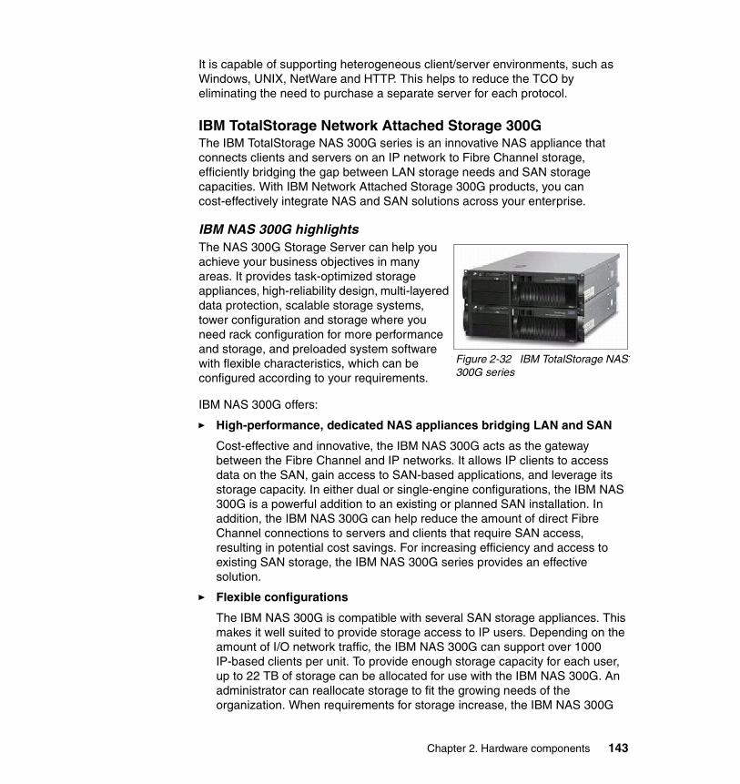
It is capable of supporting heterogeneous client/server environments, such as Windows, UNIX, NetWare and HTTP. This helps to reduce the TCO by eliminating the need to purchase a separate server for each protocol.

IBM TotalStorage Network Attached Storage 300GThe IBM TotalStorage NAS 300G series is an innovative NAS appliance that connects clients and servers on an IP network to Fibre Channel storage, efficiently bridging the gap between LAN storage needs and SAN storage capacities. With IBM Network Attached Storage 300G products, you can cost-effectively integrate NAS and SAN solutions across your enterprise.

IBM NAS 300G highlightsThe NAS 300G Storage Server can help you achieve your business objectives in many areas. It provides task-optimized storage appliances, high-reliability design, multi-layered data protection, scalable storage systems, tower configuration and storage where you need rack configuration for more performance and storage, and preloaded system software with flexible characteristics, which can be configured according to your requirements.

IBM NAS 300G offers:

� High-performance, dedicated NAS appliances bridging LAN and SAN

Cost-effective and innovative, the IBM NAS 300G acts as the gateway between the Fibre Channel and IP networks. It allows IP clients to access data on the SAN, gain access to SAN-based applications, and leverage its storage capacity. In either dual or single-engine configurations, the IBM NAS 300G is a powerful addition to an existing or planned SAN installation. In addition, the IBM NAS 300G can help reduce the amount of direct Fibre Channel connections to servers and clients that require SAN access, resulting in potential cost savings. For increasing efficiency and access to existing SAN storage, the IBM NAS 300G series provides an effective solution.

� Flexible configurations

The IBM NAS 300G is compatible with several SAN storage appliances. This makes it well suited to provide storage access to IP users. Depending on the amount of I/O network traffic, the IBM NAS 300G can support over 1000 IP-based clients per unit. To provide enough storage capacity for each user, up to 22 TB of storage can be allocated for use with the IBM NAS 300G. An administrator can reallocate storage to fit the growing needs of the organization. When requirements for storage increase, the IBM NAS 300G

Figure 2-32 IBM TotalStorage NAS 300G series


can access multiple SAN devices to provide additional storage. Compatible storage includes the ESS, FAStT200, FAStT500, FAStT700, and other vendors' devices.

Because of its flexibility, the IBM NAS 300G series provides administrators with the necessary tools to manage storage resources more efficiently. It creates a more cost-effective storage system and reduces the TCO.

By deploying the IBM NAS 300G series, access to existing SAN storage is a possible solution to the increasing demands for additional storage. The IBM NAS 300G is preloaded with Tivoli SANergy® software, which lets users access storage on the SAN at file, volume, and byte levels with increased throughput and lower overhead. The resulting high-performance link between the IP clients and the SAN helps to fully use the existing investments in both networks.

The IBM NAS 300G series provides:

– File server storage consolidation– IP clients and servers with access to SAN storage– IP clients with access to mission-critical data from the SAN– IP clients with the ability to back up critical information to the SAN

� High system availability for business continuance

The IBM NAS 300G series includes a single and a dual-engine model. The single-engine model is a good value for those who want to extend the reach of their SAN. Clustering and fail-over protection are available in the dual-engine model. The IBM NAS 300G series incorporates a variety of high-reliability and availability features to support their operation 24-hours a day, seven days a week.

Both models house hot-swappable, redundant power supplies in each engine and optionally provide multipath fail-over protection between the unit and its SAN-attached storage device. Each engine supports an optional second hard drive and RAID 1 for creating mirrored system drives to further increase system availability.

� Integrated data protection

The IBM NAS 300G series helps to safeguard the most valuable asset of an organization—its data—by providing such features as:

– Backup support using Tivoli Storage Manager and other third-party software packages

– Protection against accidental file deletions

– File restorations by clients and administrators

– Single-step volume and drive restorations by administrators


The IBM NAS 300G supports a variety of backup methods, including popular backup software such as Tivoli Storage Manager. The Tivoli Storage Manager agent and client are pre-installed on the product.

The IBM NAS 300G also offers on-disk data protection using Columbia Data Products Persistent Storage Manager (PSM), which can create up to 250 True Image views of data. Administrators can schedule the creation of these point-in-time views. With the proper permissions, users can typically restore previous file levels without administrator involvement.

Administrators can also usually restore entire drives and volumes in a single step, saving precious IT time by eliminating the need to drag and drop thousands of files back to the original location. By incorporating its own open file manager, PSM can enable safe and consistent backup of in-use files. The open file manager helps to reduce or eliminate system access issues during backup, supporting availability to data 24-hours a day, seven days a week.

For more information about IBM NAS solutions, see:

http://www.storage.ibm.com/snetwork/nas/

2.7 Additional hardware considerationsThis section looks at some additional considerations that the person who is performing the sizing may have to address.

2.7.1 Multiprocessor configurationsDifferent types of multiprocessor configurations coexist. The three major ones are described in the following sections.

Shared memory multiprocessor Figure 2-33 shows a shared memory multiprocessor environment. Shared memory multiprocessor, also known as a tightly coupled multiprocessor, has multiple processors that have their own cache and can each address the shared memory and all devices. User processes on any processor see the full system. If two or more processors access the same word in memory, hardware keeps the caches consistent and invisible to application processes. Compared to other multiprocessor types, the advantage of shared memory multiprocessors is their use of the same programming model as uniprocessors.


http://www.storage.ibm.com/snetwork/nas/

Figure 2-33 Shared memory multiprocessor environment

Shared nothing multiprocessorA shared nothing multiprocessor as shown in Figure 2-34 is where all processors have their own memory and disks. Uniprocessor programs must be changed to use the parallelism of this configuration because they must pass messages across an interconnect to use the multiple processors. The IBM RS/6000 SP is an example of this kind of architecture.

Shared nothing multiprocessors generally scale better than shared memory multiprocessors because they have no memory bus contention and no cache coherency problems among the processors.

Figure 2-34 Shared nothing multiprocessor environment

Processor

Main Memory

Cache

Processor

Cache

Processor

Cache

Processor

Cache

Processor

Memory

Processor

Memory

Processor

Memory

Processor

Memory

High-speed interconnection


Shared disk multiprocessorUnlike the shared memory multiprocessor environment, each processor on a shared disk multiprocessor has its own memory as shown in Figure 2-35. That is why the shared disk multiprocessors, like the shared nothing multiprocessors, have no memory bus contention or cache coherency problems among the processors. However, a centralized locking scheme is used to control access to the disks. This locking scheme requires changes to some applications (such as databases. It generally offsets the performance advantages of no memory bus contention or the cache coherency problem.

Figure 2-35 Shared disk multiprocessor environment

2.7.2 NUMANUMA was developed to offer better scalability for large servers. The demand for scalability has increased due to the requirements of large databases and decision support systems, such as e-business applications, where server load is a key issue.

IBM has done significant work and research on NUMA technology for many years. When Sequent® joined IBM, they added a lot of experience in NUMA performance and tuning.

There has been a steady increase in demand for systems that offer higher processor power. If the system has performance problems, the logical solution is to add additional processor power to the system, but this solution does not

Processor

Memory

Processor

Memory

Processor

Memory

Processor

Memory

Interconnect


address the issues of memory accessing that can quickly erode any performance increases of additional processor power.

Figure 2-36 shows some of the system components that limit scalability of non-NUMA architectures.

Figure 2-36 System architectures

Architecture plays an important role in how a system performs. Architecture must take advantage of the processor and marketplace technologies and offer scalability. To enhance processor throughput, the following technologies were developed:

� SMP: Share everything� MPP: Share nothing resource

There are advantages and disadvantages to both philosophies. Each is suited to different environments. With SMP, the programming model is easier.

MPP provides high performance for compute-intensive workloads. However, it requires data partitioning. Therefore, it not a good choice for running some commercial applications.

With SMP’s easy programming model, it has been very popular and over time the need for performance of SMP has increased. With SMP’s architectural limitations, you cannot simply add processors and expect the equivalent gain in performance.

Uni-processors

MicrosBus based

SMP

Chip to ChipCommunication

BusBandwidth

BusLength

MemoryInterconnect

Latency

DRAMLatency

MTAIRAM

?

Scaling limitations

High SpeedBusses

SMP

CrossbarsSMP

CC-NUMA


To take advantage of faster processors, physically shorter buses and buses with fewer central interconnects are needed to reap the benefits of memory with ever decreasing latency times.

With NUMA, the concept is to combine these areas to offer program simplicity and the flexibility of SMP while providing low-latency, high- multiprocessing for commercial applications.

Software that runs on an SMP system runs on NUMA systems. Some by their nature even run efficiently, but others need to understand the NUMA characteristics to perform well on a NUMA system. Even if certain software runs well in a large SMP, that is no guarantee it will run well in a NUMA environment.

NUMA combines the resources of a group of systems and allows sharing of data between them. For example, the memory on multiple servers appears as one.

2.7.3 Logical partitioningLogical partitioning (LPAR) is the ability to divide a physical server into virtual logical servers, each running in its own private copy of the operating system.

Though it may not seem practical, running a machine with a single LPAR, compared to full system partition mode (non-LPAR), provides for a faster system restart. This is because the Hypervisor has already provided some initialization, testing, and building of device trees. In environments where restart time is critical, we recommend that you test the single LPAR scenario to see if it meets the system recycle time objectives.

Depending on the software installed on the server, DLPAR may be available or unavailable:

� DLPAR available: With dynamic LPAR available, the resources can be exchanged between partitions without stopping and rebooting the affected partitions. Dynamic LPAR requires AIX 5L Version 5.2 for all affected partitions. The Hardware Management Console (HMC) recovery software must be at Release 3 Version 1 (or higher). In partitions running AIX 5L Version 5.1 or Linux, if available, the Dynamic Logical Partitioning menu is not available.

� DLPAR unavailable: Without dynamic LPAR, the resources in the partitions are static. DLPAR is unavailable for partitions running AIX 5L Version 5.1 or Linux, when available. When you change or reconfigure your resource without DLPAR, all the affected partitions must be stopped and rebooted to make resource changes effective.

A server can contain a mix of partitions that support dynamic LPAR along with those that do not.


Hardware Management ConsoleWith LPAR mode, an IBM HMC for pSeries is necessary. Either a dedicated 7315-C01 or an existing HMC from a pSeries 670 or 690 installation (FC 7316) can be used. If a server is used in full system partition mode (no LPARs) outside a cluster, an HMC is not required.

The HMC is a dedicated desktop workstation that provides a graphical user interface (GUI) for configuring and operating pSeries servers functioning in either non-partitioned, LPAR, or clustered environments. It is configured with a set of hardware management applications for configuring and partitioning the server. One HMC is capable of controlling multiple pSeries servers. At the time of writing, a maximum of 16 non-clustered pSeries servers and a maximum of 64 LPARs are supported by one HMC.

The HMC is connected with special attachment cables to the HMC ports of the hardware. Only one serial connection to a server is necessary despite the number of LPARs.

With these cables, the maximum length from any server to the HMC is limited to 15 meters. To extend this distance, a number of possibilities are available:

� Another HMC can be used for remote access. This remote HMC must have a network connection to the HMC that is connected to the servers.

� AIX 5L Web-based System Manager Client can be used to connect to the HMC over the network. Or the Web-based System Manager PC client can be used, which runs on a Windows operating system-based or Linux operating system-based system.

� When a 128-Port Async Controller is used, the RS-422 cables connect to a RAN breakout box, which can be up to 330 meters. The breakout box is connected to the HMC port on the server using the attachment cable. When the 15 meter cable is used, the maximum distance of the HMC can be 345 meters, providing the entire cable length can be used.

The HMC provides a set of functions that are necessary to manage LPAR configurations. These functions include:

� Creating and storing LPAR profiles that define the processor, memory, and I/O resources allocated to an individual partition

� Starting, stopping, and resetting a system partition

Note: Rebooting a running partition only restarts the operating system and does not restart the LPAR. To restart an LPAR, shut down the operating system without reboot. Then afterwards restart it again.


� Booting a partition or system by selecting a profile

� Displaying system and partition status

In a non-partitioned system, the LED codes are displayed in the operator panel. In a partitioned system, the operator panel shows the word LPAR instead of any partition LED codes. Therefore all LED codes for system partitions are displayed over the HMC.

� Virtual console for each partition or controlled system.

With this feature, every LPAR can be accessed over the serial HMC connection to the server. This is a convenient feature when the LPAR is not reachable across the network or a remote NIM installation should be performed.

The HMC also provides a service focal point for the systems it controls. It is connected to the service processor of the system using the dedicated serial link. The HMC provides tools for problem determination and service support, such as Call Home and error log notification through an analog phone line.

LPAR minimum requirementsEach LPAR must have a set of resources available. The minimum resources that are needed are:

� At least one processor per partition� At least 256 MB of main memory� At least one disk to store the operating system (for AIX, the rootvg)� At least one disk adapter or integrated adapter to access the disk� At least one LAN adapter per partition to connect to the HMC� An installation method, such as NIM, for the partition and a means of running

diagnostics, such as network diagnostics

Memory guidelines for LPARThere are a few limitations consider when planning for LPAR. Planning the memory for logical partitioning involves additional considerations. These considerations are different when using AIX 5L Version 5.1, AIX 5L Version 5.2, or Linux.

When a machine is in full system partition mode (no LPARs), all of the memory is dedicated to AIX. When a machine is in LPAR mode, some of the memory used by AIX is relocated outside the AIX-defined memory range. In the case of a single small partition on a pSeries 630 (256 MB), the first 256 MB of memory is allocated to the Hypervisor. Then, 256 MB is allocated to translation control entries Translate Control Entries (TCE) and to Hypervisor per partition page tables. And, 256 MB is allocated for the first page table for the first partition. TCE memory is used to translate the I/O addresses to system memory addresses.


Additional small page tables for additional small partitions fit in the page table block. Therefore, the memory allocated independently of AIX to create a single 256 MB partition is 768 MB (0.75 GB).

With the previous memory statements in mind, LPAR requires at least 2 GB of memory for two or more LPARs on a pSeries 630. It is possible to create a single 256 MB LPAR partition on a 1 GB machine. However, this configuration should be used for validation of minimum configuration environments for test purposes only. Other systems have different memory requirements.

You must close any ISA or integrated development environment (IDE) device before you remove any DLPAR memory from the partition that owns the ISA or IDE I/O. This includes the diskette drive, serial ports, CD-ROM, or DVD-ROM, for example.

The following rules only apply to partitions with AIX 5L:

� The minimum memory for an LPAR is 256 MB. You can configure additional memory in increments of 256 MB.

� The memory consumed outside AIX is from 0.75 GB to 2 GB, depending on the amount of memory and the number of LPARs.

� For AIX 5L Version 5.1, the number of LPARs larger than 16 GB is limited to two in a system with 64 GB of installed memory, because of the memory alignment in AIX 5L Version 5.1.

LPARs that are larger than 16 GB are aligned on a 16 GB boundary. Because the Hypervisor memory resides on the lower end of the memory and TCE resides on the upper end of the memory, only two 16 GB boundaries are available.

You must also consider the organization of the memory in a server. Every processor card has its dedicated memory range. Processor card one has the range 0 GB to 16 GB, processor card two has the range 16 GB to 32 GB, processor card three has the range 32 GB to 48 GB, and processor card four has the range 48 GB to 64 GB. If a processor card is not equipped with the maximum possible memory, there will be holes and the necessary 16 GB contiguous memory will not be present in the system. For example, in a system with three processor cards and 36 GB of memory, the memory is distributed into the ranges 0 to 12, 16 to 28, and 32 to 50. In this configuration, the only available 16 GB boundary (at 16 GB) has 12 GB of memory, which is too small for a partition with more than 16 GB of memory and AIX 5L Version 5.1.

� With AIX 5L Version 5.2, there are no predefined limits concerning partitions larger than 16 GB, but the total amount of memory and Hypervisor overhead remains a practical limit.


2.7.4 Dynamic logical partitioning (5.2.0)With the availability of the pSeries 690 server in December 2001, static LPAR was introduced to the pSeries platform. While LPAR provides a solution to logically remove and assign resources from one partition to another, you must reboot the operating system in all affected partitions and reset the partitions.

DLPAR on pSeries servers enables the movement of hardware resources (such as processors, memory, and I/O slots) from one LPAR running an operating system instance to another partition without requiring reboots and resets. With DLPAR technology the following features are enabled: dynamic reconfiguration, Dynamic Capacity Upgrade on Demand (DCUoD), and CPU sparing.

As shown in the system architecture in Figure 2-37, a DLPAR system is made up of several components. To provide the foundation for DLPAR, the following components were made DLPAR aware:

� HMC� Hypervisor� Global firmware� Local firmware� AIX

Note: To create LPARs running AIX 5L Version 5.2 or Linux larger than 16 GB, you must select the Small Real Mode Address Region check box (on the HMC, LPAR Profile, Memory Options window). Do not select this box if you are running AIX 5L Version 5.1.


Figure 2-37 pSeries DLPAR system architecture

DLPAR architecture (5.2.0)Figure 2-38 shows how DLPAR-aware components interact in an example where a user on the HMC initiates the movement of a resource from one partition to another. Here is a description of the components that are involved:

� HMC: The Hardware Management Console is the command center from which all decisions related to the movement of resources are made.

� chhwres: The chwres HMC command is where commands are issued to dynamically add and remove resources from partitions as well as move resources between partitions. You can issue this command using the HMC GUI or from a command line.

� DRM: The Dynamic Reconfiguration Manager (DRM) is an agent that is designed to deal with DLPAR-specific issues. DRM invokes AIX commands to attach or detach DLPAR capable resources.

� RMC: The Remote Monitoring and Control (RMC) handles monitoring and controlling distributed resource classes. It is a distributed framework that is designed to handle all security and connectivity issues related to networks. In conjunction with DRM, it enables the remote execution of commands to drive the configuration and unconfiguration of DLPAR-enabled resources.

� RTAS: The Run-Time Abstraction Services (RTAS) is firmware that is replicated in each partition. It operates on objects in the Open Firmware


Device Tree such as processors, logical memory blocks (LMB), I/O slots, date chips, and NVRAM. Operations include query, allocate, electronically isolate, and free resources.

� Global FW: One global firmware (FW) instance spans the entire system. The global firmware is also known as the Hypervisor. It contains the boot and partition manager, manages memory and I/O mappings, and provides a global name space for resources. It dictates the set of DLPAR-enabled resources and contains the Open Firmware device tree. AIX communicates with it through the RTAS layer.

Figure 2-38 DLPAR system architecture

DRM

RMC

DRM

RMC

RTAS RTAShypervisor/global firmware

AIX AIX

chhwres

RMC

HMC

1

2

3

4

5

6 7

8

9

10

11

12

kernel/machdd kernel/machdd

cmds cmds


The sequence of operations for the given example as provided in Figure 2-38 is explained as follows:

1. The chhwres command on the HMC calls the RMC with the request to release the given resource.

2. RMC establishes a connection through the Ethernet network to the RMC on AIX and passes the request to release the resource. The RMC connection to the partition is established at boot time.

3. RMC calls DRM with the request to release the resource.

4. DRM initiates the appropriate AIX commands to release the resource from the operating system.

5. The AIX commands invoke the appropriate functions of the kernel. The operating system attempts to stop using the specified resource. If it cannot stop using the resource, an error is returned to the user. If it can stop using the resource, the operating system isolates the resource, powers it off, and sets the status to unusable. Success is reported to the chhwres command on the HMC.

6. The chhwres command calls the global firmware and reclaims the resource.

7. The chhwres command calls the global firmware and assigns the resource to the partition.

8. The chhwres command calls RMC with the request to configure the resource.

9. RMC establishes a connection using the network to the RMC on the partition and passes on the request. The RMC connection is established at boot time.

10.RMC calls DRM with the configuration request.

11.The DRM calls the appropriate AIX commands with the request to add the resource to the operating system.

12.The AIX command initiates the appropriate operating system functions and the operating system attempts to make the specified resource usable using RTAS calls. If this operation is unsuccessful, an error is returned to the user. If the operation is successful, the operating system takes ownership of the resource and firmware removes it from its resource pool. Then the resource is powered on, not isolated, and finally configured by the operating system.

Prior to DLPAR, applications considered CPU and memory to be constant resources on a system. With DLPAR, the number of CPUs and the amount of memory can change during the runtime of the applications.

Most applications are not aware of the number of CPUs and the memory in the system. Therefore they are most likely not affected by DLPAR operations. However, some applications are aware of the amount of these system resources, and they need to handle changes to the system configuration.


There are two types of applications with respect to DLPAR operations: DLPAR-safe and DLPAR-aware applications.

A DLPAR-safe application does not fail as a result of a DLPAR operation. It may not be affected at all. Its performance may suffer or it may not scale with the addition of new resources. It may even prevent a DLPAR operation from succeeding, but it functions as expected.

A DLPAR-aware application is an application that adjusts its use of system resources to facilitate DLPAR operations. To participate in DLPAR operations, the application may either regularly poll the system topology to discover changes. Or it can register with the DLPAR application framework to receive notification of DLPAR events when they occur. The latter (registration) should be the preferred choice.

Do not use the polling model if the application has a processor dependency. It may need to unbind before the operating system attempts to reconfigure the resource. The polling model only provides notification after the DLPAR event.

Types of applications that should be made DLPAR aware are:

� Enterprise-level databases: These databases scale with the system configuration. They typically use large pinned buffer pools that scale with the physical memory and the amount of threads scales with the number of CPUs.

� System tools (performance monitors, for example): They report CPU and memory statistics.

� Multi-system level job scheduling: They schedule jobs based on the number of CPUs and memory.

� License managers: They license on a CPU basis.

DLPAR operations are non-destructive by design. That means DLPAR operations fail if the resource to be removed is locked by applications or the kernel. A DLPAR CPU remove request fails if an application is bound to the CPU being removed. This can be a bindprocessor command or Workload Manager rset type binding.

A DLPAR memory remove request fails if most of the memory in the system is pinned. AIX has the capability to dynamically migrate pinned memory so that virtually any range of memory can be removed. However, if the system cannot acquire a new pinned page, the operation fails. AIX allows approximately 80% of the system to be pinned. Therefore, programs that consume lots of pinned memory should be made DLPAR aware so that the system has adequate resource to perform memory removal. Applications pin memory through the block() and shmget(SHM_PIN) system calls.


Two interfaces are available to make an application DLPAR aware: a script-based and an API-based interface. Using the script-based approach, the administrator or software vendor installs a set of scripts that are called by the DLPAR application framework when a DLPAR event occurs. For the API-based approach, the new signal SIGRECONFIG is defined. It is sent during DLPAR events to all processes that are registered to catch this event.

The SIGRECONFIG signal is also sent (along with the SIGCPUFAIL signal for backward compatibility) in the case of a CPU Guard event. Therefore the DLPAR application framework can also be used by CPU Guard-aware applications.

In the first release of DLPAR support, the dynamic reconfiguration of I/O slots is not integrated into the DLPAR Framework in the same way that CPUs and memory is. The user cannot install DLPAR scripts or make their applications DLPAR aware by registering for a signal.

For a complete description of logical partitioning, see The Complete Partitioning Guide for IBM Eserver pSeries Servers, SG24-7039.

2.7.5 Dynamic CPU sparing and CPU Guard (5.2.0)Dynamic CPU sparing allows you to dynamically replace a CPU resource if a CPU failure is reported by Open Firmware. This CPU replacement happens in such a fashion that it is transparent to the user and to user-mode applications.

In AIX 5L Version 5.2, the CPU Guard implementation has been changed and enhanced to work in the new DLPAR Framework. The actual deallocation of the CPU resource is performed in the DLPAR Framework by the dynamic CPU removal procedure.

The DLPAR mechanism allowing the dynamic processor removal is based on leaving holes in the logical CPU ID’s sequence. This is unlike the former CPU Guard implementation where holes in logical CPU IDs are not tolerated for compatibility reasons.

The dynamic processor removal (DR) strategy is to abstract the status of the CPUs by having CPU bind IDs, which are a sequence of IDs 0 through N-1 representing only the online CPUs. This strategy provides better MCM-level affinity, breaking the assumption of uniform memory access from all CPUs by RPDP. With the dynamic processor removal approach, the load from the failing CPU is moved to a CPU that corresponds to the last CPU bind ID. Thus the failing CPU bind ID and the last CPU bind ID are swapped, leaving a hole in the logical CPU ID sequence and making the last online CPU the failing processor. Therefore, the bindprocessor system call interface, the bindprocessor command, the bindintcpu command, and the switch_cpu kernel service have


been changed to work with the CPU bind ID model instead of the logical CPU ID model.

CPU Guard dynamically removes a failing CPU, where CPU sparing replaces a CPU with a spare one under the cover. During the reconfiguration, no notifications of any kind are sent to the user, kernel extensions, or user-mode applications that are CPU Guard- or DR-aware.

Dynamic CPU sparing is supported only on systems that are loaded with appropriate CPU Guard and DLPAR-enabled firmware such as the pSeries 690 and 670 running in LPAR mode with a CPU Capacity Card present. Spare CPUs are CUoD CPUs that are not activated with a CUoD activation code.

Since CPU Guard operations are considered dynamic processor removal operations, they are serialized with all other dynamic processor removal operations. In this new environment, the second-to-last CPU can be removed, which was a restriction to the prior CPU Guard implementation.

The dynamic CPU sparing process is explained as follows:

1. Open Firmware reports predictive CPU failure.

2. The event is logged to AIX error log and reported to the kernel.

3. The SIGCPUFAIL signal is sent to the init process.

4. The init process starts the ha_star command.

5. The ha_star command determines from the ODM whether to perform CPU sparing or CPU removal.

6. The drmgr command is called to perform CPU sparing or CPU removal.

7. The end of the CPU sparing procedure is logged into the AIX error log indicating the change in the physical cpuid.

A new ODM attribute, CPU sparing, is introduced. You can set it to enable or disable with SMIT using the fast path smit chgsys.

CPU Guard default changed (5.2.0)The default feature of CPU Guard has been changed from disabled to enabled in AIX 5L Version 5.2. This only applies if the feature is supported by the system. To display the current status of CPU Guard, run the following command:

lsattr -El sys0 -a cpuguard

To change the value of CPU Guard to disabled, run the following command:

chdev -l sys0 -a cpuguard=disable


A process should be considered critical to the system if, in the case where the process is terminated, the system itself should be terminated. These are all kernel processes or processes being executed in kernel mode.

Furthermore, a process can register itself or another process as being critical to the system. To register or unregister a process, two new system calls are provided that can be called from the process environment:

pid_t ue_proc_register (pid, arg)pid_t ue_proc_unregister (pid)

In some cases, an application may want to take action before being terminated, for example, to create its own error log entry. To do so, the process should catch the SIGBUS signal with a SA_SIGINFO type of handler.

A new AIX Uncorrectable Error Gard (UE-Gard) error log entry is used by the kernel when signalling a process to terminate. This log entry contains the process ID and the signal value that caused the termination. The LABEL and RESOURCE fields in the AIX log indicate an UE-Gard event.

2.7.6 UE-Gard (5.2.0)The UE-Gard is a RAS feature that enables AIX in conjunction with hardware and firmware support to isolate certain errors that would have previously resulted in a condition where the system had to be stopped (checkstop condition). The isolated error is analyzed to determine if AIX can terminate the process that suffers from the hardware data error instead of terminating the entire system.

In the most likely case of intermittent errors, UE-Gard prevents the system from terminating. However, in the unlikely case of a permanent memory error, the system issues a checkstop eventually if the same memory is reused by a process that cannot be terminated.

pSeries Models 630, 650, 670, and 690 are supported at the time of writing.

UE-Gard is not to be confused with (dynamic) CPU Guard. CPU Guard takes a CPU dynamically offline after a threshold of recoverable errors is exceeded, to avoid system outages.

The logic for UE-Gard is shown in Figure 2-39. On memory errors, the firmware analyzes the severity and records it in an RTAS log. AIX is called from firmware with a pointer to the log. AIX analyzes the log to determine whether the error is recoverable. If the error is recoverable, then AIX resumes. If the error is not fully recoverable, then AIX determine whether the process with the error is critical. If the process is not critical, then it is terminated by issuing a SIGBUS signal with a


UE siginfo indicator. In the case where the process is a critical process, then the system is terminated as a machine check problem.

Figure 2-39 UE-Gard logic

Memory errorHardware

Firmware

AIX

Analyze error

Analyze log

Error fully recoverable ?

Affected process critical?

Terminate process

Resume Stop

RTAS log

yes

yes

no

no



Chapter 3. Software components

The software components that are supported by the pSeries server are:

� AIX� Dynamic logical partitioning (DLPAR)� Workload Manager� Linux

This chapter examines each of these components.

3


3.1 AIXAIX stands for Advanced Interactive eXecutive. It is the IBM version of UNIX. AIX was created as the premier UNIX operating system by IBM for their line of RISC technology servers in the mid 1980s. Originally, AIX was primarily based on AT&T’s UNIX System Version 2. It has evolved over the years through different versions. It has taken on characteristics of the UNIX Berkeley Software Distribution (BSD UNIX), the OSF/1 version, and versions of UNIX that have come from the Open Software Foundation (OSF, now Open Group), of which IBM was a founding member.

3.1.1 History of AIXAIX began with the release of Version 3.0 in 1990. This sections takes you through the history of releases that have since evolved.

AIX Version 3First released in February of 1990, AIX Version 3.0 through 3.2.5 was created to support the IBM Reduced Instruction Set Computing (RISC) line of POWER servers. It was the first version of AIX to offer POSIX IEEE 1003.1 1988 standards conformance, X/Open XPG3 base-level compliance, and Berkeley Software Distribution 4.3 (4.3 BSD) compatibility.

Also, the operating system, as a whole, took on new tools and enhancements not offered by other forms of UNIX.

Logical Volume ManagerThe Logical Volume Manager (LVM) introduced a hierarchical storage management system to AIX. LVM introduced the concept of “logical volumes” to AIX storage management. It allowed a more dynamic configuration of physical partitions that allowed system data to span several physical disks.

System Management Interface ToolTo provide an easier and more user friendly interface to AIX, the System Management Interface Tool (SMIT) was created as a menu-driven tool. It executes support for installation, configuration, device management, problem determination, and storage management. Through a series of interactive menus and dialogs, SMIT automatically builds, executes, and logs the appropriate AIX system commands required to execute the required operation.

Trusted Computing Base The Trusted Computing Base (TCB) within AIX offers a means to restrict access of system resources in a secure manner to authorized users and processes. TCB also allows for system auditing and event logging of suspicious system events. It


allows a system administrator to make sure that system resources are only used along specified security parameters.

Motif X Window ManagerMost types of UNIX provide some sort of graphical user interface (GUI). In early versions of AIX, this was done using the Motif X Window manager. Motif provided a fully configurable and programmable GUI to AIX. Support for Motif became integrated into the AIX window functionality.

Network File SystemAlthough it was originally only offered as a separately licensed program before AIX 3.2, the Network File System (NFS) eventually became an integral part of AIX. It was integrated into the AIX 3.2 offering. NFS allows for local mounting of non-local storage media over a TCP/IP network.

AIX Version 4In July of 1994, IBM introduced AIX Version 4. Throughout AIX Version 4, AIX saw many changes and enhancements to the system kernel. The following sections cover the changes that AIX experienced from AIX 4.1 through AIX Version 4.3.3.

Network Install ManagerNetwork installations were possible within previous versions of AIX. However, it became a formal and fully supported process with AIX Version 4 through the Network Install Manager (NIM).

NIM installs the basic operating system and other operating system components from the server onto clients within the network. NIM streamlined the installation process for AIX. This works especially on the SP hardware platform where many AIX installs can take place. NIM allows these installs to take place without constant system administrator intervention.

Journaled file systemBefore AIX Version 4.1, data was written within logical volumes to the file system in set blocks of 4096 bytes. With the introduction of a journaled file system (JFS) into AIX, support for data block fragments as small as 512 bytes was created. This allows files to more efficiently use disk space when a data file is smaller than 4096 bytes long.

Dynamic Host Configuration ProtocolSupport was added for Dynamic Host Configuration Protocol (DHCP) in AIX Version 4.1.4. DHCP is a network service under TCP/IP that allows for automatic network configuration of network clients upon startup.

Chapter 3. Software components 165

The system administrator only has to configure one server in the network with all the relevant network data. Clients can then access a host configuration automatically from this server upon bootup.

Common Desktop Environment The AIX Common Desktop Environment (CDE) replaced the Motif X Window manager as an industry standard GUI to AIX. CDE 1.0 became the default bootup desktop in AIX Version 4.1.3. It was included in both the AIX Version 4 for Clients package and AIX Version for Servers package.

Web-based System ManagerWeb-based System Manager (WebSM) enables a system administrator to manage an AIX system either locally from a graphics terminal or remotely from a PC or pSeries client.

Information is entered through the use of GUI components on the client side. The information is then sent over the network to the WebSM server, which runs the commands necessary to perform the required action.

Internet Protocol version 6 supportInternet Protocol Version 6 (IPv6) is the next generation Internet Engineering Task Force (IETF) networking protocol. It will become the industry standard network protocol for the Internet of the future.

IPv6 extends the maximum number of Internet addresses to handle the ever-increasing Internet user population. IPv6 is an evolutionary change from IPv4 and has the advantage of allowing a mixture of new and old to coexist on the same network. This coexistence enables an orderly migration from IPv4 (32-bit addressing) to IPv6 (128-bit addressing) on an operational network.

AIX 5LAIX 5L was created with the intention of creating an open standards version of UNIX compatible with 64-bit based hardware platforms. Along with being 64-bit compliant, AIX 5L also offers affinity with another open standards version of UNIX, Linux. It has binary compatibility with previous versions of AIX. AIX 5L Version 5.0 has many enhancements and additions over the previous version, AIX 4.3.3.

The release of AIX 5L includes the features that are described in the following sections.

Enhanced Journaled File SystemThe Enhanced Journaled File System (JFS2) is an enhanced and updated version of the JFS. JFS2 is intended to provide a robust, quick restart,


transaction-oriented, log-based, and scalable byte-level file system implementation for AIX environments. JFS2 has new features that include extent based allocation, sorted directories, and dynamic space allocation for file system objects. While tailored primarily for the high throughput and reliability requirements of servers, JFS2 is also applicable to client configurations where performance and reliability are desired.

Both JFS and JFS2 are available on POWER systems.

NFS statd multithreadingIn AIX 5L, the NFS statd daemon is multi-threaded. In AIX Version 4.3, when the statd daemon detects whether clients are up, it hangs and waits for a time out when a client cannot be found. If there are a large number of clients that are offline, it can take a long time to time out all of them sequentially.

With a multithreading design, stat requests run in parallel to solve the time-out problem. The server statd monitors clients and the client’s statd monitors the server if a client has multiple mounts. Connections are dropped if the remote partner cannot be detected without affecting other stat operations.

Configuration managerThe installation of new hardware has been streamlined in AIX 5L through enhancements to the configuration manager (cfgmgr). It now adds new devices in parallel. Previous versions of cfgmgr added devices sequentially as it discovered them.

Web-based System ManagerThe Web-based System Manager (WebSM) tool has the following enhancements over AIX Version 4.3.3:

� A new management console� Point-to-point multiple host management� New Java 1.3 compliance� Shell script and application programming interface (API) execution interface� Dynamic user interface� Kerberos v5 integration

The /proc file systemThe /proc file system contains a directory for each kernel data structure and active process running on the system. Each of these entries gets a Process Identification Number (PID) within the kernel memory. Now within AIX 5L, each PID gets its own directory structure within /proc.

Working with kernel data structures and processes in this manner allows a debugger or system administrator to stop and start threads within a process,


trace system calls, trace signals, and read and write to virtual memory within a process. The new /proc file system can be invaluable in debugging system processes and applications.

The /opt file systemThe /opt or “optional” directory is reserved for the installation of add-on application software packages. It is integral to AIX 5L’s new affinity with Linux applications.

Deactivating active paging spaceThis feature provides new flexibility (does not require rebooting) when changing configurations, moving paging space to another device, or dividing paging space up between drives. For earlier releases, allocated and activated paging space must stay active until the next reboot.

With this release, paging space can be deactivated without rebooting by using the new swapoff command. The new shrinkps command creates a new, temporary space, deactivates the original, and changes the original to be smaller. Then it reactivates it, deactivates the temporary space, and returns it to logical volume status.

Resource monitoring and controlResource monitoring and control (RMC), comparable to Reliable Scalable Cluster Technology (RSCT) on the SP, allows a system administrator to configure an AIX 5L system to monitor itself in terms of performance, availability, and response. The RMC subsystem comes preconfigured with 84 conditions and eight responses. They can be used “as is” or as templates for creating your own performance monitoring conditions and responses.

Native Kerberos 5 supportThe AIX 5L operating system allows the system administrator to replace the default login process with Kerberos 5 authentication. Kerberos 5, after a user has logged in their ID, acquires all appropriate network and system credentials. In previous AIX releases, the distributed computer environment (DCE) and the network information system (NIS) were supported as alternate authentication mechanisms.

AIX Version 4.3.3 added Lightweight Directory Access Protocol (LDAP) support and the initial support for specifying a loadable module as an argument for the user/group managing commands, such as mkuser, lsuser, and rmuser. This was documented only in the /usr/lpp/bos/README file.

AIX 5L now offers a general mechanism to separate the identification and authentication of users and groups. It defines an API that specifies which function entry points a module must make available to work as an identification or


authentication method. This allows for more sophisticated customized login methods beyond what is provided by the ones based on /etc/passwd or DCE.

Virtual IP address supportFor applications to access communication and network services, previous releases of AIX required applications to bind themselves to a physical network interface. With the application bound to a physical IP address, the application could become inaccessible if the IP interface went down or TCP/IP services became interrupted.

With the addition of virtual IP address (VIPA) support in AIX 5L, an application can be bound to a virtual IP address that can be routed to any accessible hardware network interface. This way, if one interface goes down, the VIPA can be routed to another interface. If done fast enough, it can prevent the loss of TCP/IP sessions. Furthermore, a VIPA can be brought down independently of the access of other running applications. This allows multiple applications to use the same interface for communication and for the virtual IPs to be brought up or down without affecting any other application’s network interface.

3.1.2 AIX kernelAt the heart of the AIX operating system is the AIX kernel. This kernel provides the ability to share system resources simultaneously among many processes or threads and users. The most important resources that the kernel manages are the processor or processors, memory, and devices. By careful design, the kernel is preemptable and pageable. It is also dynamic and extendable.

PreemptableThe kernel can be in the middle of a system call and be preempted. This preemption can signal a context switch that causes an entirely new thread of execution inside the kernel. Threads are assigned a priority by the kernel that the kernel can adjust based on certain factors, such as the length of time the thread has been running. Preemptability allows the kernel to respond to real-time processes much faster than other operating systems.

In a preemptable kernel, a higher-priority thread that becomes capable of running may preempt a low-priority thread even though it is executing kernel code. Device drivers and other interrupts can preempt processes in kernel mode. Upon its return from the interrupt, the preempted process retains control of the CPU. In contrast, processes in user mode are always preemptable. Upon its return from an interrupt, the kernel decides which process should run next, based on priority.


Pageable (demand paging)A pageable kernel means that only those parts of the kernel that are being used or referenced are kept in physical memory. Kernel pages that have not been used recently can be paged out. Some parts of the kernel are not paged out. Instead, they are pinned. An example of pinned kernel code is the interrupt processing section of the device drivers.

The kernel uses a pager daemon to keep a pool of physical pages free. It uses a Least Recently Used (LRU) algorithm. If the number of pages that are available goes below a high-watermark threshold, the pager frees the oldest LRU pages until a low-watermark threshold is reached.

In other operating systems, including some UNIX variants, the entire kernel must be loaded and pinned into memory. This feature acquires more significance when you consider that AIX functionality can be dynamically extended using kernel extensions. Therefore, while the AIX kernel may tend to be larger than other kernels, due in part to user-added functions through kernel extensions, it usually requires less physical memory to actually run.

DynamicIn AIX, kernel extensions can be added to and deleted from the kernel as needed. This allows an administrator to add new device drivers, file systems, and other kernel code at any time without recompiling the kernel. Since recompiling the kernel is not required, rebooting the system is not normally required for changes to take effect.

ExtendableKernel extensions are dynamically loadable in AIX. These extensions allow programs direct access to kernel resources for better performance.

A system programmer can add new services in AIX by using the defined kernel extension types. These extension types can be divided into four categories:

� Device drivers� System calls� Virtual file systems� Kernel processes

When properly coded, kernel extensions add extensibility, configurability, and ease of system administration to AIX. This combination of features allows the AIX kernel to be highly scalable, from the smallest of the PowerPC processors to the largest pSeries 690. It also allows for the fine tuning of an operating environment.


3.1.3 Modes of operation (execution modes)There are two modes of operation in the AIX operating system: the kernel mode and the user mode. Kernel extensions run in the kernel mode, and user applications tend to run in the user mode. Kernel mode has unlimited access to these and other functions, including additional instructions and commands. In user mode, programs have access to kernel data and global structures.

The receipt of an interrupt can cause a process or thread running in user mode to change to the kernel mode to handle the exception. An interrupt can be caused by an external signal, program error, program request, or any other unusual condition. The receipt of an interrupt causes a switch to the kernel mode and an immediate branch to a specific memory location or vector. The operating system has code at that vector to save the machine state and branch to a handler routine.

3.1.4 AIX 5L kernel subsystemsFigure 3-1 illustrates the AIX 5L kernel architecture. Within the kernel, various subsystems are dedicated to particular functions. These subsystems generally operate with a high priority in the operating system, as do most kernel processes. The following sections list the major components of the kernel.

Exception versus interrupt: These terms are often confused. An interrupt is caused by hardware, and an exception is caused by user code.


Figure 3-1 AIX 5L kernel architecture

System call interfaceThe system call interface is the primary mechanism for user-mode applications to access the kernel. This layer can be thought of as the API to the kernel. Applications make system calls to obtain information, perform operations, and access resources through the kernel.

Input/output subsystemAccess to files and directories is controlled by various layers within the input/output (I/O) layer of the AIX kernel. There are many parts of this I/O layer. The major functions contained in the I/O layer provide a consistent view to the user of any file within the operating system, whether it is a real physical file, a remote file, or even a logical file. The intent is to deal with all file types via the same system calls, such as open(), close(), read (), write(), etc.

The major functions of this layer are:

� Logical file system (LFS): The LFS provides AIX and user applications with a consistent view of all file system implementations. Physical file system types are shielded by the logical file system.

User programs Libraries

System call interface

Logical file system

Virtual file system

Physical file system

Virtual Memory Manager

Process Management Subsystem

Scheduler

User mode

Kernel mode

Hardware

Platform Abstraction Layer

Logical Volume Manager

I/O subsystem


� Virtual file system (VFS): The VFS provides a standard set of operations on entire file systems.

� Physical file system (PFS): There are different types of PFSs, such as JFS, CD-ROM file system, NFS, and so on.

� Virtual Memory Manager (VMM): The VMM provides processes with a virtual address space. It allows the creation of memory segments that are greater than the physical memory.

� Logical Volume Manager: The LVM provides the definition and management of volume groups, logical volumes, and physical volumes. This creates a virtual disk environment that can be dynamically changed.

Process management (scheduler)A thread is the smallest scheduled and dispatched entity within AIX 5L. A process which may have a single thread or a collection of threads is a self-contained entity that consists of the information required to run a program.

Process management allows many processes and their threads to exist simultaneously and share the processor. The scheduler places runnable threads on the run queue based on priority. The dispatcher is then invoked to “dispatch” the highest priority thread to the selected processor. The dispatcher is also invoked at the completion of interrupts and exceptions.

The AIX scheduler uses a time-sharing priority-based scheduling algorithm. The scheduler periodically scans the list of all active processes and threads. It recalculates process priorities based on the initial priority and the amount of processor time used. It tends to favor processes that do not consume large amounts of the processor time because the amount of processor time used by the scheduler is included in the priority recalculation equation.

Virtual memory managerVirtual memory is a mechanism by which the real memory available for use appears larger than its true size. The virtual memory system is composed of physical disk space, where portions of a process that are not currently in use are stored, as well as the system’s real memory.

The physical disk part of virtual memory is divided into three types of segments that reflect where the data is being stored:

� Local persistent segments from a local file system� Working segments in the paging space� Client persistent segments from CD-ROM, JFS2, or remote file systems

One of the basic building blocks of the AIX memory system is the segment, which is a 256 MB (228) piece of the virtual address space. Each segment is


further divided into 4096 byte pages of information. Each page sits in a 4 KB partition of the disk, known as a block. Similarly, real memory is divided into 4096 byte pages.

The VMM coordinates and manages all the activities associated with the virtual memory system. The VMM is responsible for allocating real memory page frames and resolving references to pages that are not currently in real memory.

Previous releases of AIX managed all of a system’s real memory as one large resource that was available for the programs executing in one or more CPUs to address and use through the VMM. There was one list of free memory pages. There was also a one-page replacement daemon that would help to ensure that the required pages could actually be located in system RAM.

Since systems continue to grow, AIX has improved memory management through the use of multiple free pages lists and multiple page replacement daemons. This increases the VMM concurrency since contention has been reduced in the serialization mechanisms and processes with lower latencies can now service the memory requests.

Platform Abstraction Layer The Platform Abstraction Layer (PAL®) in the kernel was introduced with AIX Version 4. It is ostensibly the hardware-control layer. This is the layer in which device drivers are accessed by the kernel. All hardware-dependent code is extracted from the kernel and placed in kernel extensions. This facilitates new hardware and device support.

3.1.5 Multitasking and multithreading supportAIX 5L is a multitasking system that uses processes and threads. A thread is an independent flow of control that operates within the same address space as other independent flows of control within a process. In previous versions of AIX, and in most UNIX systems, thread and process characteristics are grouped into a single entity called a process. In other operating systems, threads are sometimes called lightweight processes or the meaning of the word thread is sometimes slightly different.

In traditional single-threaded process systems, a process has a set of properties. In multithreaded systems, these properties are divided between processes and threads.

A process in a multithreaded system is the changeable entity and must be considered as an execution frame. It has all traditional process attributes, such as process ID, process group ID, user ID, group ID, environment, and working directory.


A process also provides a common address space and common system resources for:

� File descriptors� Signal actions� Shared libraries� Interprocess communication tools, such as message queues, pipes,

semaphores, or shared memory

A thread is the scheduled or dispatched entity. It has only those properties that are required to ensure its independent flow of control. A kernel thread is a kernel entity, such as processes and interrupt handlers. It is the entity handled by the system scheduler. A kernel thread runs within a process but can be referenced by any other thread in the system. The programmer has no direct control over these threads unless kernel extensions or device drivers are written.

A user thread is an entity used by programmers to handle multiple flows of controls within a program. The API for handling user threads is provided by a library called the threads library. A user thread only exists within a process. A user thread in process A cannot reference a user thread in process B. The library uses a proprietary interface to handle kernel threads for executing user threads. The user threads’ API, unlike the kernel threads’ interface, is part of a portable programming model. Thus, a multithreaded program developed on an AIX system can easily be ported to other systems.

User threads are mapped to kernel threads by the threads library. The way this mapping is done is called the thread model. There are three possible thread models that correspond to three different ways of mapping user threads to kernel threads:

� M:1 model� 1:1 model� M:N model

Mapping user threads to kernel threads is done using virtual processors. A virtual processor (VP) is a library entity that is usually implicit. The virtual processor looks like a real processor to the user thread. The VP behaves just as a CPU does for a kernel thread. In the library, the virtual processor is a kernel thread or a structure bound to a kernel thread.

In the M:1 model, all user threads are mapped to one kernel thread. All user threads run on one VP. The mapping is handled by a library scheduler. All user threads programming facilities are completely handled by the library. This model can be used on any system, especially on traditional single-threaded systems. Figure 3-2 illustrates this model.


Figure 3-2 M:1 threads model

In the 1:1 model, each user thread is mapped to one kernel thread; each user thread runs on one VP. Most of the user threads’ programming facilities are handled directly by the kernel threads. Each thread can be separately and independently passed out to any processor on the system for execution. Figure 3-3 illustrates this model.

Figure 3-3 1:1 threads model

VP

Library Scheduler

Thread library

UserThread

KernelThread

UserThread

UserThread

VP

Thread library

VPVP

UserThread

UserThread

UserThread

KernelThread

KernelThread

KernelThread


In the M:N model, all user threads are mapped to a pool of kernel threads and run on a pool of virtual processors. A user thread may be bound to a specific VP, as in the 1:1 model. All unbound user threads share the remaining VPs. This is the most efficient and complex thread model. The user threads’ programming facilities are shared between the threads’ library and the kernel threads. Figure 3-4 illustrates this model.

Figure 3-4 M:N threads model

By implementing a multi-threaded kernel, AIX is well suited to run in a symmetric multiprocessor (SMP) system. AIX has been optimized to run on SMP systems, and scalability on these systems is very high.

3.1.6 64-bit kernelBeginning with AIX 5L, the operating system provides a 64-bit kernel that addresses bottlenecks which may have limited throughput on 32-bit systems. POWER4 and POWER4+ systems are optimized for a 64-bit kernel, which is intended to increase scalability of RS/6000 and pSeries systems. It is optimized to run 64-bit applications on POWER4 and POWER4+ systems. The 64-bit kernel also improves scalability by allowing you to use larger sizes of physical memory. The 32-bit system is limited to 4 GB of physical memory.

In 32-bit systems, an individual program or process has 32 bits of effective address space for its own use to contain instructions and data. With 64-bit computing, applications run in a 64-bit address space. Here, an individual

Thread libraryVP

VP

Library Scheduler

UserThread

UserThread

UserThread

KernelThread

KernelThread


program’s addressability becomes measured in terabytes (TB) instead of gigabytes (GB).

Some database management programs use a large address space for scalability to maintain very large data buffers in memory. This reduces the amount of disk I/O they need to perform. Using a large address space, they can supply data to client applications at the speed needed to sustain the high transaction rate.

In certain cases, database management programs or client applications may benefit from keeping an entire database or large file immediately accessible in memory. Read-only data lends itself most readily to this scenario. Significant improvements in response time or transaction rates are possible. Certain types of applications can directly attack larger problems by organizing larger arrays of data to be computed upon. Computer simulation of a physical phenomenon, such as aircraft flight or a nuclear reaction, are frequently cited examples.

Performance of applicationsConsider the differences in performance between the following applications.

64-bit applications on a 32-bit kernelThe performance of 64-bit applications running on the 64-bit kernel on POWER4 or POWER4+-based systems should be greater than, or equal to, the same application running on the same hardware with the 32-bit kernel. The 64-bit kernel allows 64-bit applications to be supported without requiring system call parameters to be remapped or reshaped.

32-bit applications on a 64-bit kernelIn most instances, 32-bit applications on the 64-bit kernel typically have slightly lower performance than on the 32-bit kernel because of parameter reshaping. This performance degradation is typically no greater than 5%.

3.2 Workload ManagerWorkload Manager is designed to give the system administrator greater control over how the scheduler and VMM allocate CPU, physical memory, and I/O resources to processes. It can be used to prevent different jobs from interfering with each other. It can also help to allocate resources based on the requirements of different groups of users or applications.

Workload Manager is useful for large SMP systems. It is typically used for server consolidation, where workloads from many different server systems, (print, database, general user, transaction processing systems, and so on) are combined. These workloads often compete for resources and have differing


goals and service level agreements. At the same time, Workload Manager can be used in uniprocessor workstations to improve responsiveness of interactive work by reserving physical memory.

Workload Manager provides isolation between user communities with different system demands. This can prevent effective starvation of workloads with certain characteristics, such as interactive or low CPU usage jobs, by workloads with other characteristics, such as batch or high CPU usage.

Workload Manager helps system administrators create different classes of service and specify attributes for those classes. They can classify processes automatically into classes, based on the user, group, or path name of the application.

3.2.1 ClassesThe central concept of Workload Manager is the class. A class is a collection of processes (jobs) that has a single set of resource limits applied to it.

Workload Manager assigns processes to the various classes and controls the allocation of system resources among the different classes. For this purpose, Workload Manager uses class assignment rules and per-class resource shares and limits set by the system administrator. The resource entitlements and limits are enforced at the class level. This defines classes of service and regulates the resource utilization of each class of applications to prevent applications with different resource utilization patterns from interfering with each other.

Hierarchy of classesWorkload Manager allows system administrators to set up a hierarchy of classes with two levels by defining superclasses and subclasses. See Figure 3-5. A class can be either a superclass or a subclass. The difference between superclasses and subclasses is the resource control (shares and limits):

� At the superclass level, the determination of resource entitlement (based on the resource shares and limits) is based on the total amount of each resource managed by Workload Manager available on the system.

� At the subclass level, the resource shares and limits are based on the amount of each resource allocated to the parent superclass.


Figure 3-5 Hierarchy of classes

The system administrator (the root user) can delegate the administration of each superclass to a superclass administrator (a non-root user). They allocate a portion of the system resources to each superclass. Then they allow superclass administrators to distribute the allocated resources among the users and applications they manage.

Workload Manager supports 32 superclasses (27 user defined plus five predefined). In turn, each superclass can have 12 subclasses. Depending on the needs of the organization, a system administrator can decide to use only superclasses or both superclasses and subclasses. An administrator can also use subclasses only for some of the superclasses.

Each class is given a name by the Workload Manager administrator who creates it. A class name can be up to 16 characters long and can only contain uppercase and lowercase letters, numbers, and underscores (_). For a given Workload Manager configuration, the names of all the superclasses must be different from one another. The names of the subclasses of a given superclass must also be different from one another. Subclasses of different superclasses can have the same name. The fully qualified name of a subclass is superclass_name.subclass_name.

The term class in the remainder of this section applies to both subclasses and superclasses. The following sections describe both super and subclasses in greater detail. They also discuss the backward compatibility that Workload Manager provides to configurations of its first release.

Workload Manager superclassA superclass is a class with subclasses associated with it. No process can belong to the superclass without also belonging to a subclass, either predefined or user assigned. A superclass has a set of class assignment rules that determine which

Superclass_B Superclass_CSuperclass_A

Subclass_1 Subclass_2 Subclass_3

Superclass_B Superclass_CSuperclass_A

Subclass_1 Subclass_2 Subclass_3


processes to assign to it. A superclass also has a set of resource limitation values and resource target shares that determine the amount of resources that can be used by processes that belong to it. These resources are divided among the subclasses based on the resource limitation values and resource target shares of the subclasses.

Up to 27 superclasses can be defined by the system administrator. In addition, five superclasses are automatically created to deal with processes, memory, and CPU allocation:

� Default superclass: The default superclass is named Default and is always defined. All non-root processes that are not automatically assigned to a specific superclass are assigned to the Default superclass. Other processes can also be assigned to the Default superclass by providing specific assignment rules.

� System superclass: This superclass has all privileged (root) processes assigned to it if they are not assigned by rules to a specific class. It also has the pages that belong to all system memory segments, kernel processes, and kernel threads. Other processes can be assigned to the system superclass. The default is for this superclass to have a memory minimum limit of 1%.

� Shared superclass: This superclass receives all the memory pages that are shared by processes in more than one superclass. This includes pages in shared memory regions and pages in files that are used by processes in more than one superclass (or in subclasses of different superclasses).

Shared memory and files used by multiple processes that belong to a single superclass (or subclasses of the same superclass) are associated with that superclass. The pages are placed in the shared superclass when a process from a different superclass accesses the shared memory region or file.

This superclass can have only physical memory shares and limits applied to it. It cannot have shares or limits for the other resource types, subclasses, or assignment rules specified. Whether a memory segment shared by the processes in the different superclasses is classified into the shared superclass, or remains in the superclass it was initially classified into, depends on the value of the localshm attribute of the superclass the segment was initially classified into.

� Unclassified superclass: The processes in existence at the time Workload Manager is started are classified according to the assignment rules of the Workload Manager configuration being loaded. During this initial classification, all the memory pages attached to each process are charged either to the superclass to which the process belongs (when not shared or shared by processes in the same superclass) or to the shared superclass, when shared by processes in different superclasses.


However, there are a few pages that cannot be directly tied to any processes (and thus to any class) at the time of this classification. This memory is charged to the unclassified superclass. An example is pages from a file that has been closed. The file pages remain in memory, but no process owns these pages. Therefore, they cannot be charged to a specific class. Most of this memory ends up being correctly reclassified over time, when it is either accessed by a process, or freed and reallocated to a process after Workload Manager is started.

There are a few kernel processes, such as wait or Irud, in the unclassified superclass. Although you can apply physical memory shares and limits to this superclass, Workload Manager commands do not allow you to set shares and limits or specify subclasses or assignment rules on this superclass.

� Unmanaged superclass: A special superclass named Unmanaged is always defined. No processes are assigned to this class. This class is used to accumulate the memory usage for all pinned pages in the system that are not managed by Workload Manager. The CPU utilization for waitprocs is not accumulated in any class. This is deliberate. Otherwise, the system would always seem to be at 100% CPU utilization. This can be misleading for users who are looking at Workload Manager or system statistics. This superclass cannot have shares or limits for any other resource types, subclasses, or assignment rules specified.

Workload Manager subclassesA subclass is a class associated with exactly one superclass. Every process in the subclass is also a member of the superclass. Subclasses only have access to resources that are available to the superclass. A subclass has a set of class assignment rules that determine which of the processes assigned to the superclass will belong to it. A subclass also has a set of resource limitation values and resource target shares that determine the resources that can be used by processes in the subclass. These resource limitation values and resource target shares indicate how much of the superclass’s target (the resources available to the superclass) can be used by processes in the subclass.

The system administrator or by the superclass administrator can define up to 10 out of a total of 12 subclasses for each superclass. In addition, two special subclasses, default and shared, are always defined in each superclass:

� Default subclass: The default subclass is named Default and is always defined. All processes that are not automatically assigned to a specific subclass of the superclass are assigned to the Default subclass. You can also assign other processes to the Default subclass by providing specific assignment rules.

� Shared subclass: This subclass receives all the memory pages used by processes in more than one subclass of the superclass. This includes pages


in shared memory regions and pages in files that are used by processes in more than one subclass of the same superclass.

Shared memory and files used by multiple processes that belong to a single subclass are associated with that subclass. The pages are placed in the shared subclass of the superclass only when a process from a different subclass of the same superclass accesses the shared memory region or file. There are no processes in the shared subclass. This subclass can only have physical memory shares and limits applied to it. It cannot have shares or limits for the other resource types or assignment rules specified.

3.2.2 TiersTier configuration is based on the importance of a class relative to other classes in Workload Manager. There are 10 available tiers from zero to nine. Tier zero is the most important, and tier nine is the least important. As a result, classes that belong to tier zero have resource allocation priority over classes in tier one, classes in tier one have priority over classes in tier two, and so on. The default tier number, if the attribute is not specified, is zero.

Tiers apply at both the superclass and subclass levels. Superclass tiers help to specify resource allocation priority between superclasses. Subclass tiers help to do the same between subclasses of the same superclass. No relationship exists between tier numbers of subclasses of different superclasses.

Figure 3-6 Relationship between classes

Tier 1

Tier 0

Tier 1

Tier 0

Subclass_1

Tier 1

Subclass_3

Superclass_A

Superclass_B

Tier 0

Subclass_1

Subclass_2

Subclass_2

Subclass_3

Tier 1

Tier 0

Tier 1

Tier 0

Subclass_1

Tier 1

Subclass_3

Superclass_A

Superclass_B

Tier 0

Subclass_1

Subclass_2

Subclass_2

Subclass_3


Tier separation, in terms of prioritization, is more enforced in AIX 5L than in the previous release. A process in tier one never has priority over another process in tier one. There is no overlapping of priorities in tiers. It is unlikely for classes in tier one to acquire any resources if the processes in tier zero consume all the resources.

3.2.3 Class attributesTo create a class, different attributes are necessary to have an accurate and well-organized group of classes. The attributes of classes are:

� Class name: Up to 16 characters long; can contain only uppercase and lowercase letters, numbers, and underscores (_)

� Tier: Number between zero and nine for class priority ranking

� Inheritance: Specifies whether a child process inherits the class assignment from its parent

� Adminuser, admingroup (superclass only): Used to delegate the administration of a superclass

� Authuser, authgroup: Used to delegate the right to manually assign a process to a class

� Resource set: Used to limit the set of resources to which a given class has access in terms of CPUs (processor set)

� Localshm: Specifies whether memory segments that are accessed by processes in different classes remain local to the class they were initially assigned to, or if they go to the shared class

3.3 LinuxIBM is focusing on Linux because of the increased market share that Linux is gaining, the rapid market changes, and the client demands. Linux is a stable and reliable development and deployment platform for Internet applications. Its low cost and broad platform support allow applications to be developed on commodity hardware and deployed across a wide range of systems.

Linux for personal computing environments can be acquired at no cost as a download from the Internet. The kernel and most of the extensions are available as source code and can be improved by anyone who is willing to contribute.

Linux is a popular operating system for Web servers and dedicated networking functions, such as Web infrastructure, file-and-print serving, firewalls, directory serving, e-mail serving, and so on. It is rapidly gaining a position in application and database servers. Linux has also gained acceptance as an embedded


operating system for new Internet, file server, and other application appliances. Currently both SuSE and RedHat are available.

3.3.1 Linux for pSeriesLinux for pSeries is a key element of the IBM Eserver Linux strategy. The commitment of IBM to provide Linux for pSeries was announced as part of the IBM Eserver launch in October 2000. IBM intends to increase its growing server momentum by leveraging the power of open source in general and Linux in particular to offer new options and value to its clients. For pointers to other documents that more fully address the overall Linux strategy of IBM, see 3.3.4, “Other related information and links” on page 186.

Today, Linux is strong at the low end of the scalability range, while pSeries has carved out a leadership position in the mid-range and high-end of the enterprise server space. As Linux becomes more mature in enterprise reliability, availability and scalability, Linux for pSeries grows more compelling. As Linux scalability grows, so do the workloads for which it can be deployed. IBM is working closely with the Linux community to increase performance, scalability, reliability, and serviceability to match the strengths of pSeries servers.

Linux for pSeries is also compelling for solutions that require a 64-bit architecture or the high performance floating-point capabilities of the POWER4+ processor.

LPAR capabilities of the pSeries (see 3.3.3, “Logical partitioning” on page 186) make it possible to run one or more instances of Linux with AIX. This offers a low-risk way to begin developing and deploying Linux operating system-ready applications as desired while retaining the enterprise-ready capabilities of AIX for mission-critical or highly-scalable workloads. Since Linux doesn’t currently scale to efficiently handle large SMP systems, LPAR allows you to partition large pSeries systems to run Linux workloads.

3.3.2 Linux and AIXThe AIX platform is, and will continue to be, the premier operating system from IBM for pSeries systems. To enhance the interoperability between Linux and AIX, IBM has ported a collection of open source and GNU software tools from the Linux world and bundled them into a toolbox for users of AIX. The AIX Toolbox for Linux Applications is the first step in IBM efforts to provide AIX and Linux interoperability.

For clients of AIX, it opens up a range of open sourced Linux applications, development tools, and utilities. Linux users running Intel architecture systems have the option to move up to more powerful systems. And for Linux developers, it introduces a way to expand the target for applications to AIX.


The toolbox contains a collection of open source and GNU software that works with both AIX 4.3.3 and AIX 5L. Some of those applications include precompiled versions of the Gnome and KDE desktop environments and system utilities (including Emacs, Samba, shells, and GNU base utilities) and application development tools such as compilers libraries and software installers.

After they are developed and compiled, the original Linux source applications become native AIX applications. This means that they can take advantage of the same scalability and performance like any other AIX application. These applications are AIX binaries. They cannot be run on Linux for pSeries without being recompiled. Similarly, applications developed on Linux for pSeries do not run in binary form on AIX.

3.3.3 Logical partitioningLinux is supported running in one or more static LPARs on all pSeries systems which support LPAR. AIX and Linux can run concurrently in separate partitions on an LPAR-enabled system in any combination (for example, zero or more Linux partitions along with zero or more AIX partitions). This enables a client to consolidate workloads from several separate servers onto a single system. Since partitioning is controlled by the Hypervisor firmware and the Hardware Management Console (HMC) for pSeries, AIX is never required to run Linux.

Dynamic LPAR is currently not supported by Linux. However, Linux partitions can be created on systems enabled for DLPAR. The Linux partition appears to be unavailable on the HMC and cannot be changed dynamically. To reconfigure Linux in an LPAR environment, you must stop Linux first, reconfigure the partition, and then restart Linux. Future releases of Linux may support DLPAR.

3.3.4 Other related information and linksFor more information, see the following documents:

� IBM Eserver pSeries Linux on pSeries Overview

http://www-1.ibm.com/servers/eserver/pseries/linux/whitepapers/linux_pseries.pdf

� IBM Eserver pSeries Facts and Features, G320-9878


� Linux RAS for IBM Eserver pSeries

https://techsupport.services.ibm.com/server/Linux_on_pSeries/images/Linux_RAS.pdf





http://www-1.ibm.com/servers/eserver/pseries/linux/whitepapers/linux_pseries.pdf

Chapter 4. Benchmarks

This chapter introduces the industrial standard benchmarks. It explains characteristics of each benchmark and the relationship between industry standard benchmarks and sizing.

In particular, it covers:

� Online transaction processing (OLTP) benchmarks� Business intelligence (BI) benchmarks� e-business benchmarks� High Performance Computing (HPC) benchmarks� Independent software vendor (ISV) benchmarks

4


4.1 Introduction to benchmarksThere are several reasons to study benchmark tests. The most well-known reason is to compare performance of different computers because clients need to know which system is better for their applications when they are deciding to buy a system. However, it is difficult to find an absolute measurement because, nowadays, computers are complex systems in which many components influence the overall performance of the system. System performance especially depends on the kind of application software that is running on the system.

Benchmarks are necessarily abstract and simplified models of application environments. For this reason, benchmarks represent a good measuring tool to compare different systems rather than a precise tool for capacity planning for a given client application environment. No benchmark can fully characterize the performance of a system in a true production environment because:

� The behavior of benchmark applications is essentially constant on a given system. Real applications, when executed several times, almost invariably have different inputs, and consequently exhibit different behavior each time.

� Benchmarks are executed under ideal circumstances. The benchmark is typically the only application that is executed on a system dedicated to a single purpose. For this reason, system overheads, such as paging and context switches, are lower than in actual production use of a processor. Benchmark processors are often equipped with the latest and greatest memory and disk subsystems. They may include features that may not match exactly a system that is of interest to a client. In this sense, benchmarks represent the upper limit of system performance.

Nonetheless, there is useful information we can gather from benchmark results. Benchmarks provide some insight into the performance of a computer:

� A computer that performs well on all benchmarks in a given class, such as floating-point-intensive codes with data structures that are too large to fit into cache memory, is likely to perform well in all applications that share these characteristics.

� A processor that performs well in throughput benchmarks (where many instances of many applications are run) tends to perform better in a true production environment than one that doesn’t perform well in this context.

� If you fully understand the benchmarks scenario, transaction characteristics, and metrics, and you know your application and transaction characteristics, you can use the benchmark results as a source of the rule of thumb information for your system sizing.

The benchmarks we discuss here are derived using particular, well configured, development-level computer systems. Actual system performance may vary and


depend upon many factors, including system hardware configuration and software design and configuration. Benchmark results highly depend upon workload, specific application requirements, and systems design and implementation. Therefore, do not use benchmark results as a substitute for a specific client application benchmark when critical capacity planning or product evaluation decisions are contemplated.

The best approach is to reach a deeper understanding of the benchmark. Compare its model (user interaction, database design, database size, transaction complexity, processing requirements, storage/backup tests) with the relevant application environment. If there is a rough match, the benchmark data may be a useful and relevant tool to compare different systems and can be a rough guideline to size your system.

This chapter describes the major industry standard benchmark briefly. To help you understand and use them, each benchmark is grouped by characteristics.

4.2 OLTP benchmarksOLTP is a class of program that facilitates and manages transaction-oriented applications. It typically does this for data entry and retrieval transactions in a number of industries, including banking, airlines, mail order, supermarkets, and manufacturers. OLTP transactions are processed immediately on computer systems. OLTP benchmarks are designed to measure the system performance and capability of those kinds of workloads.

4.2.1 TPC-C benchmarkTPC benchmark C (TPC-C) is an OLTP workload. It is a mixture of read-only and update-intensive transactions that simulate the activities found in complex OLTP application environments. It does so by exercising a breadth of system components associated with such environments, which are characterized by:

� The simultaneous execution of multiple transaction types that span a breadth of complexity

� Online and deferred transaction execution modes

� Multiple online terminal sessions

� Moderate system and application execution time

� Significant disk input/output (I/O)

� Transaction integrity: Atomicity, Consistency, Isolation, Durability (ACID) properties

� Nonuniform distribution of data access through primary and secondary keys

Chapter 4. Benchmarks 189

� Databases consisting of many tables with a wide variety of sizes, attributes, and relationships

� Contention on data access and update

Metrics and usageThe performance metric reported by TPC-C is a business throughput that measures the number of orders processed per minute. Multiple transactions are used to simulate the business activity of processing an order. The performance metric for this benchmark is expressed in transactions-per-minute-C (tpmC). To be compliant with the TPC-C standard, all references to tpmC results must include the tpmC rate, the associated price-per-tpmC, and the availability date of the priced configuration.

These specifications express implementation in terms of a relational data model with conventional locking scheme. However, the database may be implemented using any commercially available database management system (DBMS), database server, file system, or other data repository that provides a functionally equivalent implementation.

TPC-C uses terminology and metrics that are similar to other benchmarks, originated by TPC or others. Such similarity in terminology does not in any way imply that TPC-C results are comparable to other benchmarks. The only benchmark results comparable to TPC-C are other TPC-C results that are compliant with the same revision.

Despite the fact that this benchmark offers a rich environment that emulates many OLTP applications, this benchmark does not reflect the entire range of OLTP requirements. In addition, the extent to which a client can achieve the results reported by a vendor highly depends on how closely TPC-C approximates the client application. The relative performance (rPerf) of systems derived from this benchmark does not necessarily hold for other workloads or environments. We do not recommend extrapolations to any other environment.

Benchmark results highly depend upon workload, specific application requirements, and systems design and implementation. Relative system performance varies as a result of these and other factors. Therefore, be careful to use TPC-C benchmark in case the capacity planning is critical or product evaluation decisions are contemplated.

In TPC-C, throughput is defined as the number of new-order transactions per minute that a system generates while the system is executing four other transaction types (payment, order-status, delivery, and stock-level). All five TPC-C transactions have a certain user response time requirement, with the new-order transaction response time set at five seconds. Therefore, for a 150,000 tpmC number, a system is generating 150,000 new-order transactions


per minute while fulfilling the rest of the TPC-C transaction mix workload. This means, for example, that for every 10 new-order transactions, the required transaction mix yields approximately 10 payment transactions, and one each of delivery, order-status, and stock level.

The price/performance metric is expressed in price-per-tpmC ($/tpmC). The cost that the $/tpmC is based on is the cost of the computer or host system. It also encompasses all of the cost dimensions for an entire system environment that the user may purchase. This cost includes communications equipment, software (transaction monitors and database software), operating system, computer systems (server and client), backup storage, and maintenance for a five-year period. Therefore, if the total system cost is $7,500,000 U.S. and the throughput is 150,000 tpmC, the price/performance is derived by dividing the price of the entire system by the performance (150,000 tpmC), which equals $50 per tpmC.

TPC-C is also a convenient benchmark for symmetric multiprocessing (SMP) systems. The tpmC rates for SMP systems are listed by number of processors.

The performance metric for the TPC-C benchmark is expressed in throughput as measured in transactions per minute (tpmC).

TPC-C is most likely to be used to compare systems in a commercial environment. Determining whether the TPC-C benchmark is applicable to a specific application or environment is extremely difficult. Although this benchmark offers a rich environment that emulates many OLTP applications, it does not reflect the entire range of OLTP requirement. In addition, the extent to which a client can achieve the results reported by a vendor highly depends on how closely TPC-C approximates the client application. The relative performance of systems derived from this benchmark does not necessarily hold the same for other workloads or environments. We do not recommend extrapolations to any other OLTP environment, but if necessary, use caution.

For more information about this benchmark, values, and systems tested, see:

http://www.tpc.org/tpcc/default.asp

4.3 Business intelligence benchmarksBI has leveraged the functionality, scalability, and reliability of modern database management systems to build constantly larger data warehouses and to use

Note: In most cases in clients workloads, the CPU part is much higher than the small, well-tuned TPC-C application.


http://www.tpc.org/tpcc/default.asp

data mining techniques to extract business advantage from the vast available enterprise data. Knowledge management technologies, while less mature than BI, are now capable of combining today’s content management systems and the Web. They use vastly improved searching and text mining capabilities to derive more value from the explosion of textual information.

The amount of business data is increasing exponentially. In fact, it doubles every two to three years. More information means more competition. In the age of the information explosion, executives, managers, professionals, and workers all need to make better or faster decisions. Now, more than ever, time is money. BI provides an easy-to-use, sharable resource that is powerful, cost-effective, and scalable to your needs. BI benchmarks is designed to measure the system performance and capability of those kinds of workloads.

4.3.1 TPC-H benchmarkTPC-H is an ad-hoc decision support benchmark that represents decision support environments. It is ad-hoc in the sense that queries are random. Therefore no caching benefits influence the benchmark results. Given this, the query times can be quite long since you cannot tune the database for the query.

The benchmark consists of a suite of business related ad-hoc and concurrent data modifications. TPC-H evaluates the performance of a decision support system that performs complex queries (more complex than OLTP transactions) on large volumes of data with a high degree of complexity.

TPC-H is composed of power and throughput runs. They should be executed under the same conditions:

� Power test: Measures the raw query execution power of the system when connected with a single active user.

� Throughput test: Measures the ability of the system to process the most queries in the least amount of time.

Systems today are used for both scale-up (supporting more users and higher throughput) and speed-up (making a single task faster, reducing response time) of a workload. The power metric demonstrates the speed-up while the throughput metrics shows the scale-up capacity of the system.

The queries and the data populating the database were chosen to have broad industry-wide relevance, while maintaining a sufficient degree of ease of implementation. This benchmark illustrates decision support systems that:

� Examine large volumes of data� Execute queries with a high degree of complexity� Give answers to critical business questions


TPC-H evaluates the performance of various decision support systems by executing sets of queries against a standard database under controlled conditions. The TPC-H queries:

� Give answers to business questions

� Simulate generated ad-hoc queries (such as via a point-and-click graphical user interface (GUI))

� Are far more complex than most OLTP transactions

� Include a rich breadth of operators and selectivity constraints

� Generate intensive activity on the part of the database server component of the system under test

� Are executed against a database that complies with specific population and scaling requirements

� Are implemented with constraints derived from staying closely synchronized with an online production database

The TPC-H operations are modeled on a typical production system as follows:

� The database is continuously available 24 hours-a-day, seven days-a-week, for ad-hoc queries from multiple end users and data modifications against all tables, except possibly during infrequent (for instance, once a month) maintenance sessions.

� The TPC-H database tracks, possibly with some delay, the state of the OLTP database through on-going refresh functions that batch together a number of modifications that impact some part of the decision support database.

� Due to the world-wide nature of the business data stored in the TPC-H database, the queries and the refresh functions may be executed against the database at any time. In addition, this mix of queries and refresh functions is subject to specific ACID requirements because queries and refresh functions may execute concurrently.

� To achieve the optimal compromise between performance and operational requirements, the database administrator can set, once and for all, the locking levels and the concurrent scheduling rules for queries and refresh functions.

Metrics and usageThe performance metric reported by TPC-H is called the TPC-H Composite Query-per-Hour Performance Metric (QphH@Size). It reflects multiple aspects of the capability of the system to process queries. These aspects include the selected database size against which the queries are executed, the query processing power when queries are submitted by a single stream, and the query throughput when queries are submitted by multiple concurrent users.


The minimum database required to run the benchmark holds business data from 10,000 suppliers. It contains almost 10,000,000 rows representing a raw storage capacity of about 1 GB. Compliant benchmark implementations may also use one of the larger permissible database populations (for example, 100 GB, 300 GB, 1 TB and so on).

The TPC-H Price/Performance metric is expressed as $/QphH@Size. To be compliant with the TPC-H standard, all references to TPC-H results for a given configuration must include all required reporting components. You must not compare different size databases.

If a system costs $300,000 U.S. and the TPC-H Price/Performance metric is $1000 per QphH@100GB, then the Price/Performance is $300 (300000 divided by 1000).

The TPC-H database must be implemented using a commercially available DBMS and the queries executed via an interface using dynamic SQL. The specification provides for variants of SQL, since implementers are not required to implement a specific SQL standard in full.

TPC-H uses terminology and metrics that are similar to other benchmarks originated by the TPC and others. Such similarity in terminology does not, in any way, imply that TPC-H results are comparable to other benchmarks. The only benchmark results comparable to TPC-H are other TPC-H results that are compliant with the same revision.

The purpose of this benchmark is to reduce the diversity of operations in an information analysis application. It retains the application’s essential performance characteristics, namely the level of system utilization and the complexity of operations. A large number of queries of various types and complexities must be executed to completely manage a business analysis environment.

Many of the queries are not of primary interest for performance analysis because of the length of time the queries run, the system resources they use, and the frequency of their execution. The queries that are selected exhibit the following characteristics:

� A high degree of complexity� Use a variety of access patterns� Are of an ad-hoc nature� Examine a large percentage of the available data� All differ from each other� Contain query parameters selected at random across query executions


These selected queries provide answers to the following classes of business analysis:

� Pricing and promotions� Supply and demand management� Profit and revenue management� Client satisfaction study� Market share study� Shipping management

For additional information about this benchmark, values and systems tested, see:

http://www.tpc.org/tpch/default.asp

4.4 e-business benchmarksThe term e-business is derived from such terms as “e-mail” and “e-commerce”. It is the concept of conducting business on the Internet. It includes buying and selling as well as servicing clients and collaborating with business partners. Companies use the Web to buy parts and supplies from other companies, to collaborate on sales promotions, and to conduct joint research. Exploiting the convenience, availability, and world-wide reach of the Internet, many companies have already discovered how to use the Internet successfully.

The e-business benchmark is designed to evaluate the capability for e-business especially, for example, for Java and Web server performance.

4.4.1 TPC-W benchmarkTPC Benchmark W (TPC-W) is a transactional Web benchmark. The workload is performed in a controlled Internet commerce environment that simulates the activities of a business-oriented transactional Web server. The workload covers a range of system components associated with such environments, which are characterized by:

� Multiple online browser sessions

� Dynamic page generation with database access and update

� Consistent Web objects

� The simultaneous execution of multiple transaction types that span a breadth of complexity

� Online transaction execution modes

� Databases consisting of tables with a variety of sizes, attributes, and relationships


http://www.tpc.org/tpch/default.asp

� Transaction integrity (ACID properties)

� Contention on data access and update

The application portrayed by the benchmark is a book store on the Internet with a client browse and order scenario. Clients visit the company Web site, the store front, to look at products, find information, place an order, or request the status of an existing order. The majority of visitor activity is to browse the site. Some percentage of all visits results in submitting a new order. In addition to using the system as a store-front, it is also used for administration of the Web site. Administration includes modification to the store-front.

Multiple Web interactions are used to simulate the activity of a book store. Each interaction is subject to a response time constraint. The store size is chosen from among a set of given scale factors, which is the number of items in inventory and varies from 1,000 items to 10,000,000 items.

The following functions, if used in the benchmark, must be provided by commercially available products and be transparent to the application program:

� Multiplexing� Routing� Load balancing� Caching

The transparency requirement means that the application must not have code that directly references these functions during the measurement interval. To implement the electronic commerce function, you may use commercially available products or implementation-specific programs.

The electronic commerce function must include, at a minimum, the following capabilities as defined in this specification:

� Secure Socket Layer (SSL)� Shopping cart� Credit card verification� Secure online payment authorization

Although these specifications express implementation in terms of a relational data model with a conventional locking scheme, the database may be implemented using any commercially available DBMS, database server, file system, or other data repository that provides a functionally equivalent implementation. The terms table, row, and column are used in this document only as examples of logical data structures.


Metrics and usageThe performance metric reported by TPC-W is the average number of Web interactions processed per second. An average is used because some interactions are faster than others. For example, loading a home page is faster than other interactions. The TPC-W primary metrics are the Web interactions per second (WIPS) rating and system cost per WIPS. WIPS can be sustained by the system under test (SUT), which is the collection of servers that provide the TPC-W e-commerce solution. The cost per WIPS is essentially the cost of the SUT divided by the WIPS rate.

TPC-W simulates three different profiles by varying the ratio of browse to buy, primarily shopping (WIPS), browsing (WIPSb), and Web-based ordering (WIPSo). All references to WIPS (WIPSb, WIPSo) results must include the primary metrics, which are the WIPS rate, the associated price per WIPS ($/WIPS), and the availability date of the priced configuration.

The purpose of this benchmark is to reduce the diversity of operations found in an Internet commerce application while retaining the application’s essential performance characteristics. These are namely the level of system utilization and the complexity of operations. A large number of functions must be performed to manage an environment that supports browse and order processing.

A representative set of functions are included. Many other functions are not of primary interest for performance analysis. They are proportionally small in terms of system resource utilization or in terms of frequency of execution. Although these functions are vital for a production system, they merely create unnecessary diversity in the context of a standard benchmark and are omitted in TPC-W.


http://www.tpc.org/tpcw/default.asp

4.4.2 SPEC JBB2000 benchmarkSPECjbb2000 focuses to measure Java server performance for business applications. Java business benchmark (JBB) is helpful in predicting the performance and scalability of Java-based business solutions. It illustrates the Java engine effectiveness and how efficiently each processor, RAM, and disks are performing.

SPECjbb2000 benchmark highlights include:

� Emulation of a three-tier system, the most common type of server-size Java application today

� Business logic and object manipulation, the work of middle tier


http://www.tpc.org/tpcw/default.asp

� Clients replaced by driver threads

� Database storage by binary trees of objects

� Increasing amounts of workload applied, providing a graphical view of scalability

The SPECjbb2000 benchmark models a wholesale company, with warehouses that serve various districts. It emulates this processing with a three-tier client/server model:

1. Clients initiate information requests or orders. These requests are simulated by random input from terminal processes. It assumes that each warehouse has one terminal input.

2. These requests are processed using the business logic instructions programmed into the Java application.

3. A database is accessed to obtain the information needed to fulfill the client’s request. This database is represented by data stored in a tree-like structure held in memory. Each warehouse contains roughly 25 MB of data stored in the database.

The SPECjbb2000 process in Figure 4-1 shows benchmarks for three and five warehouses, respectively. The processes for each benchmark run are performed in a single Java environment. When running the benchmark, as the number of warehouses increase, the number of lightweight processes or threads increase, as does the size of the database.

Figure 4-1 SPECjbb2000 benchmark process

Metrics and usageA measurement is taken on the middle tier. It captures the rate at which business operations are performed per second (Ops/s). The SPECjbb2000 metric is an average number for peak performance throughputs.

Inquiry

Update

Create

Delete

Warehouseterminals

Businesslogic

Warehousedata

Warehouseterminals

Businesslogic

Warehousedata

Three warehouses Five warehouses

Inquiry

Update

Create

Delete


SPECjbb2000 performs a functional and performance test for Java platforms. It exercises the implementations of the Java Virtual Machine (JVM), Just-In-Time (JIT) compiler, threads, and some aspects of the operating system. It also measures the performance of CPUs, caches, memory hierarchy, and the scalability of processors and servers.

The SPECjbb2000 benchmark only measures performance using a single Java environment. It is also totally self-contained, because it stores all the data in memory. Therefore the benchmark does not take disk and network I/O into consideration. A “real-world” application needs to address these additional performance parameters.

SPECjbb2000 dispatches units of work against each processor. No interaction between processors for shared data takes place, and no network or disk I/O is required. Each system completes its unit of work and the result is accumulated and reported. This means that each additional processor adds to the accumulated total of the result and causes absolutely no overhead to the other processors. SPECjbb2000 is not a “real world” benchmark and should be considered along with other benchmarks that reflect real-world workloads.

In addition, most of the 64-bit JVM implementations support very large memory, so garbage collection does not occur during the benchmark. The value of the benchmark is as a measure of JVM effectiveness and what a single system is capable of delivering.

SPECjbb2000 does not use many Java software functions including Enterprise JavaBeans (EJBs), Servlets, or JavaServer Pages (JSPs).


http://www.spec.org/jbb2000

4.4.3 SPECweb99 benchmarkThe SPECweb99 benchmark is designed to measure a system’s ability to act as a Web server answering static and dynamic page requests. The features of Specweb99 include:

� Standardized workload, agreed by major players in world-wide Web (WWW) market

� Full disclosures available on this Web site

� Stable implementation with no incomparable versions

� Measurement of simultaneous connections rather than Hypertext Transfer Protocol (HTTP) operations


http://www.spec.org/jbb2000

� Simulation of connections at a limited line speed

� Dynamic GETs, as well as static GETs; POST operations

� Keepalives (HTTP 1.0) and persistent connections (HTTP 1.1)

� Dynamic ad rotation using cookies and table lookups

� File accesses more closely matching today’s real-world Web server access patterns

� An automated installation program for Microsoft Windows NT and UNIX installation scripts

� Inter-client communication using sockets

This benchmarks runs a multithreaded HTTP load generator on a number of driving “client” systems that perform static and dynamic GETs of a variety of pages from, and perform POSTs to, the SUT.

The SPECweb99 workload simulates the accesses to a Web service provider, where the server supports the home page for several different organizations. Each home page is a collection of files ranging in size from small icons to large documents or images. As in the real world, certain files within the home page are more popular than others. Dynamic GETs simulate the common practice of “rotating” advertisements on a Web page. POSTs simulate entry of user data into a log file on the server, such as may happen during a user registration sequence.

SPECweb99 consists of both static and dynamic workloads. The dynamic workload in SPECweb99 is based on two prevalent features of commercial Web servers: advertisement and user registration. Increasingly, Web servers also use browser-specific information to tailor pages and advertisements to the viewer.

There are four kinds of dynamic content requests in the SPECweb99 benchmark:

� Standard Dynamic GET� Standard Dynamic Get with CGI� Dynamic GET with Custom Ad Rotation� Dynamic POST

The Standard Dynamic GET and Standard Dynamic GET with CGI requests simulate simple advertisement rotation on a commercial Web server. Many Web servers use dynamic scripts to generate content for advertisements on Web page “on the fly”. This allows them to rotate the advertisements in real time so that the same space can be sold to different clients. The file containing the script is invoked as an executable program.

The Standard Dynamic GET with CGI request uses a non-persistent implementation so that a new process is created each time a request is received (for example, fork for UNIX and CreateProcess for Windows NT).


The Dynamic GET with Ad Rotation scheme models the tracking of users and presentation of customized advertisements based on user preferences. In the SPECweb99 implementation, a user ID number is passed as a cookie along with the ID number of the last ad seen by that user. The user’s User Personality record is retrieved and compared against demographic data for ads in the custom advertisement database, starting at the record after the last advertisement seen. When a suitable match is found, the advertisement data is returned in a cookie. In addition to the cookies, the request contains a file name to return. Depending on the name of the file to return, it is either returned as is, or it is scanned for a template string and returned with the template filled in with customized information.

The Dynamic POST request models user registration at an Internet Service Provider (ISP) site. In the benchmark, the POST data and some other information are written to a single ASCII file, called post.log. All POST requests contain a cookie value that is written into the post.log and sent back to the requester with a Set-Cookie header. Table 4-1 shows the request distribution that is used.

Table 4-1 Workload request percentage

The workload is based on the analysis of server logs from several popular Internet servers and some smaller Web sites. The workload defines four classes of files which are accessed. They have file sizes of less than 1 KB, 1 to 10 KB, 10 to 100 KB, and 100 KB to 1 MB. There are nine files in each class, with sizes distributed evenly through the range for that class. The access patterns to the files were determined from the analysis of the Web server logs. Within each class, non-linear distributions exist of accesses, reflecting the fact that certain files are more popular than others. Table 4-2 shows the file access distribution.

Request Percentage

Static GET 70

Standard Dynamic GET 12.45

Standard Dynamic GET with CGI 0.15

Dynamic GET with Ad Rotation 12.6

Dynamic POST 4.8

Total 100


Table 4-2 File sizes per class and frequency of access

Recent studies have shown that file accesses on a server follow a Zipf distribution. For an example, see:

http://www.useit.com/alertbox/zipf.html

Therefore, the SPECweb99 directory and within-class accesses are generated using the Zipf distribution function. The resulting overall distribution is close to actual measured distributions on real servers.

Metrics and usageThe performance metric of SPECweb99 benchmark is also called SPECweb99. The SPECweb99 metric represents the maximum number of simultaneous connections that a Web server can support while meeting specific throughput and error rate requirements. The connections are made and sustained at a specified maximum bit rate with a maximum segment size. They are intended to more realistically represent conditions that are seen on the Internet during the lifetime of this benchmark.

SPECweb99 was not designed as a capacity planning tool. However, it provides information about how Web servers handle this specific workload. The workload uncovers several key components of a good Web server, including LAN performance, processing power, and memory bandwidth, to name a few.

Do not compare the SPECweb99 metric with the SPECweb96 metric expressed in HTTP ops/sec or any other benchmark metric.


http://www.spec.org/web99

4.5 High Performance Computing benchmarksUsually, High Performance Computing requires massive amounts of computational power-power that enables trillions of calculations to occur within a

Class File size Frequency of access

Class 0 0 KB to 1 KB 35%



Class 3 100 KB to 1 MB 1%


http://www.spec.org/web99

http://www.useit.com/alertbox/zipf.html

second. It achieves the peak performance and productivity needed to run increasingly complex scientific and engineering applications. These are quite different with the commercial benchmarks.

To measure HPC-related system power properly, some special benchmarks for HPC environments are needed. HPC benchmarks are designed for this situation and to measure overall system performance and specific system components, for example CPU, memory, compiler, and MPI.

4.5.1 SPEC CPU2000 benchmarkSPEC CPU2000 is a benchmark that measures computer performance for CPU-intensive computing. SPEC CPU2000 contains two sets of benchmarks. SPEC CPU2000 focuses on compute-intensive performance, which means these benchmarks emphasize the performance of:

� The computer processor (CPU)� The memory architecture� The compilers

SPEC CPU2000 is made up of two subcomponents that focus on two different types of compute intensive performance:

� CINT2000 for compute-intensive integer performance� CFP2000 for compute-intensive floating point performance

SPEC CPU2000 is not intended to stress other system components, such as disk drives, networking, and graphics, which are not included in the benchmarks. However, these components may affect a system configured in a particular way.

Metrics and usageSPEC CPU2000 incorporates run and reporting rules for baseline and optimized results for both CINT2000 and CFP2000 benchmarks. Rates are calculated by timing from the start of the first copy of each code to the completion of the last copy of each code.

Metrics are defined as:

� Base: Base metrics refer to restricting the number of options on the compiler to try to represent typical use. Four flags are allowed that are generally recognized as safe. They are used for all the benchmarks in the same language in a suite.

� Peak: Peak metrics allow almost any compiler option. However, options may not name specific variables or functions.

� Non-rate or speed: These benchmarks run one program at a time, although this execution can use multiple processors, if the compiler supports this.


� Rate: Rate benchmarks execute more than one copy of each program at one time to measure throughput of a homogeneously loaded system.

There are four metrics for CINT2000 for integer compute-intensive performance comparisons:

� SPECint2000 / SPECint_rate2000

This metric is produced from the geometric mean of 12 normalized ratios (one for each integer benchmark) when compiled with aggressive optimization for each benchmark. This is a peak metric. Almost any compiler option is allowed, except those that name specific variables or functions.

SPECint2000 executes one program at one time. SPECint_rate2000 executes more than one copy of each program at one time.

� SPECint_base2000 / SPECint_rate_base2000

This metric is produced from the geometric mean of 12 normalized ratios (one for each integer benchmark) when compiled with conservative optimization for each benchmark. This is a base metric. The compiler is limited to four options.

SPECint_base2000 executes one program at a time. SPECint_rate_base2000 executes more than one copy of each program at one time.

There are four metrics for CFP2000 for floating point compute-intensive performance comparisons:

� SPECfp2000 / SPECfp_rate2000

This metric is produced from the geometric mean of 14 normalized ratios (one for each integer benchmark) when compiled with aggressive optimization for each benchmark. This is a peak metric. Almost any compiler option is allowed, except those that name specific variables or functions.

SPECfp2000 executes one program at one time. SPECfp_rate2000 executes more than one copy of each program at one time.

� SPECfp_base2000 / SPECfp_rate_base2000

This metric is produced from the geometric mean of 14 normalized ratios (one for each integer benchmark) when compiled with conservative optimization for each benchmark. This is a base metric. The compiler is limited to four options.

SPECfp_base2000 executes one program at a time. SPECfp_rate_base2000 executes more than one copy of each program at one time.

The ratio for each benchmark is calculated using a SPEC-determined reference time and the actual run time of the benchmark.


Baseline reports are mandatory for reported results and restrict the number of compiler optimization that can be used for performance testing. Reporting of optimized results is not mandatory.

Performance measurement for system speed and throughput is provided by SPEC CPU2000. The speed at which a system completes all of the CPU2000 benchmarks is provided by SPECint2000. The measurement of the number of tasks that a computer can complete in a given amount of time is provided by SPECint_rate2000.

CINT2000 and CFP2000 are based on compute-intensive applications provided as source code. CINT2000 contains 11 applications written in C and one in C++ (252.eon) that are used as benchmarks. CFP2000 contains 14 applications (six Fortran-77, four Fortran-90, and four C) that are used as benchmarks.


http://www.spec.org/cpu2000

4.5.2 LINPACK benchmarkLINear algebra PACKage (LINPACK) is the name of a library of subroutines for linear algebra calculations. It is also the name of a widely used benchmark that measures the performance of computers when solving a particular system of linear equations. The LINPACK library was superseded by the Linear Algebra PACKage (LAPACK) library. However, the name LINPACK still applies to the performance benchmark (even if the computations are done using the LAPACK library code). The LINPACK benchmark includes three versions of benchmarks:

� Linpack Fortran n=100 benchmark: This benchmark solves a 100 x 100 system of linear equations. The ground rules for running this benchmark are that you cannot make any changes to the Fortran code, not even to the comments. Only compiler optimization can be used to enhance performance.

� Linpack n=1000 benchmark1000 (also known as LINPACK Toward Peak Performance (TPP)): This benchmark solves a 1000 x 1000 system of linear equations. The ground rules for running this benchmark are more relaxed in that you can specify any linear equation solve you want, implemented in any language. This is still a popular version of the benchmark for uniprocessors, but it is too small to be useful on parallel computers.

� LINPACK NxN (also known as LINPACK HPC or LINPACK Parallel): This benchmark solves an N x N system of linear equations. The value N can be quite large so that many processors can be applied with good parallel scalability. This benchmark attempts to measure the best performance of a system in solving a system of equations.


http://www.spec.org/cpu2000

This benchmark is used as the single figure of merit for the “Top 500 List” which reports twice a year on the 500 most powerful supercomputers in the world. For information about this list, see:

http://www.top500.org

Metrics and usageThe LINPACK benchmarks indicate performance in the unit of millions of floating-point operations per second (MFLOPS). For massively parallel processors (MPPs), values are usually reported in billions of floating-point operations per second (GFLOPS).

The LINPACK 1000 and LINPACK NxN benchmarks represent the highest attainable performance level that a computer is likely to deliver. They are typically implemented by the various system vendors in ways that use caches effectively and attain excellent parallel scalability. The results are difficult to compare with real-world scientific and technical applications in general without platform-specific code optimization.

For additional information about this benchmark, values and systems tested, see the following Web sites:

http://www.netlib.org/linpackhttp://www.netlib.org/benchmark/performance.ps

4.6 ISV benchmarksISV application benchmarks are created by such individual companies as SAP, PeopleSoft, Oracle, Baan, Siebel, and J.D. Edwards. They allow clients to size ISV applications on different vendor’s hardware. They also help to answer such questions as “How many users will it support?” and “How much throughput should be expected?” Each ISV controls the publishing rules for their own applications.

4.6.1 SAP Standard Application benchmarksSAP Standard Application benchmarks test and prove the scalability of the mySAP Business Suite. The benchmark results provide basic sizing recommendations for clients by testing new hardware, system software components, and RDBMS. They allow for the comparison of different system configurations.


http://www.top500.org

http://www.netlib.org/linpack

http://www.netlib.org/benchmark/performance.ps

The benchmark suite The original SAP Standard Application benchmarks are available for many SAP components. Originally introduced to strengthen quality assurance, the SAP Standard Application benchmarks can help to test and verify scalability, concurrency and multi-user behavior of system software components, RDBMS, and business applications. All performance data relevant to system, user, and business applications are monitored during a benchmark run. They can help to compare platforms and offer basic input for sizing recommendations.

This section explains some popular benchmarks. For additional benchmark information, see:

http://www.sap.com/benchmark

Sales and Distribution benchmarkThe SAP Sales and Distribution (SD) benchmark offers a good demonstration of scalability. The SD benchmark, one of the most CPU-intensive benchmarks, has become a de facto standard for performance testing for SAP’s platform partners and in the Enterprise Resource Planning (ERP) environment.

The SD benchmark consists of the following transactions:

1. Create an order with five line items (transaction VA01). 2. Create a delivery for this order (VL01).3. Display the client order (VA03). 4. Change the delivery (VL02) and post goods issue. 5. List 40 orders for one sold-to party (VA05). 6. Create an invoice (VF01).

The SD benchmark follows the steps outlined in Table 4-3.

Table 4-3 SD benchmark steps

Step Task Step Task

0 Logon 14 Select sales order

1 Main screen 15 Select items

2 Call/nav01 (Create client order) 16 Call /nlt03 (Create transfer order)

3 Enter order and organization data 17 Save transfer order

4 Enter client and material 18 Call /nlt12 (Confirm transfer order)

5 First level characteristic value assignment

19 Confirm transfer



The workload distribution of the SD benchmark environment can be broken into three main activity categories:

� Database (14%)� Update (16%)� Dialog (70%)

Of all the SAP benchmarks, the SD benchmark places one of the highest loads on the database server. For this reason, only a limited amount of additional hardware enables full CPU utilization of the database server. The SD benchmark is referred to more often than the other SAP benchmarks when quoting SAP performance capabilities.

SAP Application Performance StandardThe SAP Application Performance Standard (SAPS) is a hardware independent unit that describes the performance of a system configuration in the SAP environment. It is derived from the SD Standard Application benchmark, where 100 SAPS are defined as 2,000 fully business processed order line items per hour. In technical terms, this throughput is achieved by processing 6,000 steps (screen changes), 2,000 postings per hour in the SD benchmark, or 2,400 SAP transactions.

Fully business processed in the SD Standard Application Benchmark means the full business process of an order line item: creating the order, creating a delivery

6 Second level characteristic value assignment

20 Call /nso01 (SAP Office-Inbox)

7 Second level characteristic value assignment

21 Select Workflow-Inbox

8 Control of resulting price 22 Start goods issue via workflow

9 Create assembly order 23 Call /nvf01 (Create invoice)

10 Call/nmf44 (Make-to-Order Backflush)

24 Save delivery note

11 Enter sales order data 25 Logoff or start process again

12 Save 26 Logoff

13 Call/nvl01 (Create a delivery)

Steps 2 through 24 are repeated n times (23 dialog steps with a minimum of 230 seconds/duration). Business aspect: One run corresponds to full assemble-to-order scenario for one item.

Step Task Step Task


note for this order, displaying the order, changing the delivery, posting a goods issue, listing orders, and creating an invoice.

Using SAPS for sizingFor example, if a sizing table for a portal suggests a configuration of 1,000 SAPS, you can check the SD benchmark table for a sample configuration. If you set the sort order in the SAPS column, you see a number of benchmark tests that can give you an idea about which configurations are likely to fulfill your requirements.

Advanced Planner and Optimizer standard application benchmark suite The SAP Advanced Planner and Optimizer (APO) benchmark suite consists of three benchmarks.

Demand Planning Demand Planning (DP) capabilities enable supply chain partners to forecast and plan demand in consideration of historical demand data, causal factors, marketing events, market intelligence, and sales objectives. Results from the planning process can be automatically fed to other nodes of the supply chain. In the benchmark, SAP use mass processing. This allows you to create demand forecasts for large numbers of products while optimizing system resources. All mass processing jobs run concurrently in the background.

For the Demand Planning benchmark, SAP assumes that every 2,000 clients buy five hundred products resulting in one million characteristic combinations (2,000 clients x 500 products). Since demand planning considers the last two years to plan for the next two years, the total number of time buckets (weeks) is 208 (4 x 52). Therefore the total number of considered data records is 208 million. The number of automatically aggregated characteristic combinations (combination of products and distribution centers) is 100,000 (in each distribution center, all products are available). The results of the benchmark are demand figures that result in actual demand.

The Supply Network Planning benchmarkWith the Supply Network Planning (SNP) solution, organizations can create a close match between supply and demand. SAP APO integrates purchasing, manufacturing, distribution and transportation into one consistent model. By modeling the entire supply network and related constraints, SAP APO can synchronize activities and plan material flow throughout the entire supply chain. The results are feasible plans for purchasing, manufacturing, inventory, and transportation alike.

SAP APO includes functionality to enable organizations to dynamically determine how and when inventory should be distributed. The system draws on


the data universally available in liveCache (a high-performance memory-based computing technology) to optimize deployment plans based on available algorithms, as well as user rules and policies. In the benchmark, SAP uses mass processing. Mass processing allows you to run heuristic planning for large numbers of product-location combinations. All mass processing jobs run concurrently in the background.

This benchmark covers the demand of the distribution centers that were created by the demand planning run. The benchmark covers three layers:

� The distribution center that have the demand� Plants that produce material� Suppliers to the plants

The Production Planning benchmarkThe component Production Planning and Detailed Scheduling (PP/DS) enables you to plan and optimize multisite production while simultaneously taking into account product and capacity availability. PP/DS is designed to plan critical products, for example, with long replenishment lead times or that are produced on bottleneck resources.

The Production Planning Benchmark uses heuristics to solve specific planning tasks for selected objects (depending on the focus of planning: products, operations, resources or line networks). It uses a particular planning procedure algorithm. Heuristic is a method of problem-solving in Production Planning and Detailed Scheduling. It uses rules that are determined by experience or intuition rather than by optimization.

This benchmark creates client demands in each production plant and uses the Production Planning Run to fulfill this demands. The benchmark covers:

� Plants that produce materials� Suppliers to the plants



4.6.2 Oracle Applications Standard benchmarkThe Oracle Applications Standard benchmark (OASB) is a comparable standard workload. It demonstrates the performance and scalability of Oracle Applications and provides metrics for the comparison of the performance of Oracle Applications on different system configurations.



The OASB is focused on ERP applications, simulating realistic client scenarios using a selection of the most commonly used Oracle Applications modules. Definitions of transactions that compose the benchmark load are obtained through collaboration with implementation consultants. They represent typical client workloads, with both OLTP and batch components.

The database used in the benchmark is designed to represent amounts of information that are typical of mid-market type businesses, whose annual revenues range from $100 million to $500 million U.S. This database is provided with the benchmark kit and is common to all platforms on which the benchmark is available.

Definitions of transactions that compose the OASB workload were obtained through collaboration with functional consultants. They represent typical client workloads, with batch transactions representing 25% of the total workload. Table 4-4 describes the OASB workload.

Table 4-4 OASB workload

As a result, the metrics reported are user count and average response time. The user count measures the number of concurrent Oracle Applications users that the system can sustain while response times are kept under a predefined maximum value. User processes are defined by the type of transactions they execute. Each user maintains a minimum transaction-per-hour rate. Neither transaction rates or the workload mix vary with increased system load or response times.

Benchmark suites are simplified models that simulate the more complex activities of real client production environments. Therefore, use caution when applying benchmark results to answer specific sizing questions in a client scenario.

Workload Description

A Oracle Financial Applications1. Accounts Payables (AP)2. Account Receivable (AR)3. Fixed Assets (FA)4. General Ledger (GL)

B Oracle Supply Chain Management Applications1. Inventory (Inv)2. Order Entry (OE)3. Purchase Orders (PO)

C 18 OLTP transactions

D 7 batch jobs


However the OASB enables system vendors to acquire experience and increase their expertise and understanding of the Oracle Applications product suite. Vendors can work with clients to compare the specific needs of their real application environment using the benchmark model. With this information, they can infer the appropriate sizing recommendations that match the expected load requirements of their production environment.


http://www.oracle.com/apps_benchmark/index.html

4.6.3 Siebel platform sizing and performance program benchmarkThis benchmark provides performance and scalability characteristics of the Siebel 7 e-business Application Suite on various operating systems and database platforms. You can use this information as an aid for system planning and sizing to support business requirements.

The test simulates real-world requirements of a large organization with several thousand concurrent users from the call center (sales and service representatives), partner organizations (Partner Relationship Management), and clients (Web sales and Web service) community. It also simulates the requirements of users supporting application services such as work assignment (Siebel Assignment Manager) and business process management (Siebel Workflow). The test also simulates integration with legacy systems (Siebel EAI MQ Series Adapter) and Web systems (Siebel EAI HTTP Adapter).

Business transactionsA total of 11 cases of complex business transactions are executed simultaneously for several thousand concurrent users. Between each user operation, there are a few seconds of think time.

The applications and solutions that are part of the Siebel 7 e-business Application Suite are:

� Siebel Call Center

– Incoming call creates a sales opportunity, quote, and order.– Incoming call creates a service request, client profile, and activity plan.– Service agent investigates and solves the service request.

� Siebel Partner Relationship Management

– Partner creates an account, contact, service request, and partner profile.– Partner creates an opportunity and activities and assigns a sales team.– Partner searches for service requests and enters a new action for a

service request.


http://www.oracle.com/apps_benchmark/index.html

� Siebel Interactive Selling Suite

– User browses a product catalog for several items.

– User browses a product catalog, places an item in shopping cart, and reviews their account profile.

– User browses a product catalog, execute complex search, and purchases a product.

� Siebel eService

– User logs a new service request and reviews open service requests.– User searches for service centers and sends e-mail.

The database is roughly 110 GB in size and comprises 10,000 accounts. It simulates clients with large transaction volumes and data distributions that represent the most common client data shapes. The DBMS was not allowed to have more than 1 GB of buffer space to prevent the database from being cached, simulating a real client environment. End users were simulated using stress tools, such as Mercury Interactive Load Runner. They drive the load with predefined weightings in the 11 scenarios, along with call center scripts driving 66% of the load.

While the clients are running, a fixed set of loads is not client driven. There are four server-based workloads: EAI HTTP, EAI MQSeries®, Workflow Manager, and Assignment Manager.

MQSeries drives 400,000 messages through Siebel Application Servers with a goal of at least 150 messages per second. EAI HTTP drives an equivalent load of at least 200 requests a second. Clients drive the workflow load with 500 load runner clients at roughly a rate of 30 transactions per second with a think time in the range of 5 seconds to 55 seconds (or an average of 30 seconds) between user operations. Finally, Assignment Manager processes 5,000 assignments roughly every minute. This set of tests fuels roughly another 25% database load at the database level. Independent application servers isolate the server-based traffic from the client load. The load is fixed, so that as we scale clients, no changes to the load occur to the server-based load.

For results, the number of users, average operation response time (sec), and business transactions throughput/hour per business transaction are measured while meeting the required key performance indicators (KPIs) defined by Siebel for certification by Siebel. Response times are measured at the Web server and not the end user. This depends on the network latency and bandwidth between Web server and browser, and the time for browser rendering.


http://www.siebel.com/products/performance_benchmark/index.shtm


http://www.siebel.com/products/performance_benchmark/index.shtm

4.7 Relative performanceWorkloads have shifted over the last several years. IBM is committed to providing clients with a relative system performance metric that reflects those changes. IBM publishes the rPerf measurement for the pSeries family of UNIX servers. It combines several different measures of total system’s commercial performance and consider the demands on a Web server in today’s environment.

rPerf is an estimate of commercial processing performance relative to other pSeries systems. It is derived from an IBM analytical model that uses characteristics from IBM internal workloads, TPC, and SPEC benchmarks. The rPerf model is not intended to represent any specific public benchmark results and should not be used in that way.

The model simulates such system operations as CPU, cache, and maximum memory available. The model does not simulate disk or network I/O operations. Although the model uses general database and operating system parameters, the model does not reflect specific database or AIX version or release.

rPerf estimates are calculated based on systems with maximum memory, the latest levels of AIX 5L, and other pertinent software. Actual performance varies based on configuration details. The pSeries 640 is the baseline reference system and has a value of 1.0. Although rPerf may be used to compare estimated IBM UNIX commercial processing performance, actual system performance may vary. It depends on many factors including system hardware configuration and software design and configuration.

Note: All performance estimates are provided “as is” and no warranties or guarantees are expressed or implied by IBM. Buyers should consult other sources of information, including system benchmarks, to evaluate the performance of a system they are considering buying. For more information about rPerf, contact your local IBM office or IBM authorized reseller.

Information in this document concerning non-IBM products was obtained from the suppliers of these products, published announcement material, or other publicly available sources including vendor Internet home pages, the SPEC home page, the Transaction Processing Performance Council (TPC) home page, and the Netlib home page.

IBM has not tested these products and cannot confirm the accuracy of performance, compatibility or any other claims related to non-IBM products. For questions about the capabilities of non-IBM products, contact the supplier of those products.


Part 3 Sizing pSeries systems

This part builds on the concepts that are related to sizing that were introduced in Chapter 1, “Overview, concepts, and approach” on page 3. It applies these concepts to the sizing of pSeries systems.

Part 3



Chapter 5. General sizing

This chapter explains how to perform general sizing with little or no specific application knowledge and only basic details about the application, users, workload, and data volumes. This chapter applies the basics of sizing from Chapter 1, “Overview, concepts, and approach” on page 3, to several sizing examples using a number of tools.

In performing these examples, we apply several rules of thumb automatically using a spreadsheet. This spreadsheet is the Balanced System Guideline, which is key to general sizing.

5


5.1 Where to locate the Balanced System GuidelineThe Balanced System Guideline spreadsheet is only available to IBM employees and IBM Business Partners. You can download it as explained here:

� For IBM employees: Go to the IBM System Sales internal Web site and search System Sales for BSG.

� For IBM Business Partners: Go to the PartnerInfo Web site. Then go to System Sales and search System Sales for BSG. Do not search the PartnerInfo Web site as a whole because it is difficult to find detailed documents at this level.

� For other users: Contact your local IBM representative or IBM Business Partner to obtain the Balanced System Guideline spreadsheet.

5.2 Six golden sizing principlesThere are six underlying principles of the Balanced System Guideline. They help to demystify the basics of how the spreadsheet works, so that you can follow what is happening.

The six principles of sizing are listed here and explained in more detail in the following sections.

5.2.1 Correct processor configurationThe processor configuration and sizing are critical. After you realize the configuration and sizing, the other components are relatively simple to determine.

5.2.2 Balanced systemsYou must size all systems to yield a reasonably balanced system in regard to processor, memory, and disk. This allows for balance from the top down and bottom up:

� The processor or processors must be powerful enough to make efficient use of the memory (caching data for later processing) and to keep the disks busy doing useful work reading information and saving the results.

� The opposite is also true. The disks must be fast enough to feed data into the memory subsystem and the memory to feed the main processor caches fast enough to keep the processors operating at maximum efficiency.


But what ratio should you use? These are determined but examining production systems at IBM Client sites and by tests performed in IBM Benchmark Centers around the world. Based on these results and findings, we developed several rules of thumb and use them in the Balanced System Guideline spreadsheet.

5.2.3 CPU magic number calculationsTo calculate the magic number for CPU power for a transaction, use the equation in Figure 5-1.

Figure 5-1 CPU magic number calculation

Figure 5-2 shows an example of 1000 users doing 60 transactions per hour (one a minute) on a 10 rPerf system using 75% of the CPU.

Figure 5-2 CPU calculation example

This example shows that it takes 0.45 seconds of processor time on a one rPerf system to run each transaction. This is called the CPU magic number.

5.2.4 Estimating CPU powerTo calculate the estimated CPU power required for a workload, use the equation in Figure 5-3.

Figure 5-3 Calculating estimated CPU power

Figure 5-4 shows an example with 1000 users at 60 transactions per hour per user and using the 0.45 magic number.

CPU rPerf x CPU Utilization x 3600

Users x Transactions-per-hour-per-userCPU seconds per transaction =

10 x 0.75 x 3600

1000 x 60= 0.45

Users x Transactions-per-hour-per-user x magic number

3600= Est. CPU Power

Chapter 5. General sizing 219

Figure 5-4 Estimated CPU power example

Since the processor would be 100% busy and highly unlikely to give a good response time etc., you would have to add a safety margin. Normally, 75% is used as a target CPU busy, so 7.5 becomes the estimated 10 CPU power rating.

From this result, you can recommend a suitable pSeries model and processors.

5.2.5 Estimating memory sizingAt a simple level, the Balanced System Guideline indicates a memory size for different workloads for a given estimated CPU power rating. At a detailed level, simple calculations are performed based on four memory uses:

� Core system

– AIX, daemons, and basic file systems– Uses a standard number

� Per user memory

– To run processes for users or batch tasks– Needs to be multiplied by the number of users in the system– Is best measured but can be guessed based on experience

� Disks Cache

– For database-like applications– Can be recommended by the vendor based on data volumes– Measured on other systems of similar data volumes– Estimated as a proportion of the data volumes

� Application binary size

– Should be measured

5.2.6 Estimating disk sizingAt a simple level, the Balanced System Guideline indicates disk sizing for different workloads. Although the opposite often occurs, from the disk sizing, you can recommend the estimated CPU power rating, which is allowed for by the Balanced System Guideline.

At a detailed level, if disk I/O rates for the transaction are measured (either physical or logical), then the disk recommendation can be based on operations

1000 x 60 x 0.45

3600= 7.5


per second rather than purely on disk size. Disks have a known maximum operations per second value. This allows you to calculate the number of disks for a given workload.

Sizing based on data size is becoming more error prone due to ever increasing disk sizes.

5.3 The Balanced System Guideline overviewThis section takes you through the Balanced System Guideline spreadsheet. It also provides examples of its use.

5.3.1 Problems with sizingAccurate sizing can be difficult because of:

� Insufficient details about the requirements from clients

� A lack of information about the application and the workload it generates on behalf of users

� The many forms that sizing requests and questions come in

� A variety of responses needed

� Different levels of accuracy

Fortunately, there are many tools (sections or sheets) within the Balanced System Guideline that help in the majority of simple sizing requests.

5.3.2 Assumptions: Prerequisites for using the spreadsheetTo use the Balanced System Guideline spreadsheet, you must:

1. Obtain the Balanced System Guideline spreadsheet.2. Unzip the spreadsheet with a suitable ZIP tool.3. Have and start the Microsoft Excel spreadsheet program.4. Load the Balanced System Guideline spreadsheet.

Depending on your setup, Excel may prompt you to specify whether you want to Disable Macros or Enable Macros. You must click Enable Macros.

Important: There is no “one size fits all” for general sizing. You must find the appropriate tool or part of a for the job.


The bulk of the spreadsheet is simple. There are some named fields, and the workload setup buttons use simple scripts to copy data in to the workload fields.

5.3.3 Spreadsheets: Pros and consThe Balanced System Guideline spreadsheet was developed by technical specialists to help them size systems. It was made generally available and developed further over the past five years.

After several implementations, the spreadsheet was found to be most practical for many reasons:

� After a sizing is finished, you can save the spreadsheet for future reference.� You can send the spreadsheet to requesters to double check or refine details.� You can perform experiments and make additions.� Most people have spreadsheet software available on their personal computer.� It looks professional and well thought out.

The down side to using the spreadsheet is that:

� You must have the correct spreadsheet and the latest version. At the time of writing, the version is Microsoft Excel 2002.

� The Balanced System Guideline may be updated without your knowledge. Therefore, you may be running an out-of-date version.

� New versions may include newly announced pSeries models, corrections to formulae, and new functions or features.

� You can enter too much information in the spreadsheet cells and corrupt the answers.

� You cannot hide secret rules of thumb. Because it is a spreadsheet, all formulas, rules of thumb, etc. are available to the end user of the spreadsheet. This is different from a canned binary executable where the formulas, rules of thumb, etc. are hidden in the program and the tool provides an answer.

� Sizing seem highly accurate when it is not. The number may be seen as accurate to three decimal places, when it is in fact plus or minus 20%.

Tip: Check regularly for updates.

Tip: Save a master (unchanged) copy of the Balanced System Guideline. Start with this copy for each sizing request. Use Save as so you don’t overwrite the master copy.


� If data is entered incorrectly or in the wrong units, it is difficult to identify and the answers may be meaningless. Some sanity checks are provided but they require experience to identify mistakes.

� Extensive use of the rPerf CPU power rating may not fit the workload type.

5.3.4 The Balanced System Guideline sectionsThe Balanced System Guideline contains several sheets that are grouped into the following categories:

� Introduction

This category contains only the Introduction sheet. It contains version details, a few definitions, and general hints and tips.

� Performance and balanced systems

This category includes the following sheets:

– Balanced: This sheet contains reference data about the current pSeries systems and the performance numbers.

This sheet also uses simple rules of thumb to suggest sensible (balanced) systems in terms of processors, memory, disks, and adapters for normal systems such as a relational database system (RDBMS). It is independent of the database vendor.

You can change the workload so that it models online transaction processing (OLTP), simple Web servers using Common Gateway Interface (CGI), Business Intelligence (BI), or application servers.

– LPAR (logical partitions): This sheet allows the calculations of estimated rPerf numbers for LPARs with a range of numbers of processors.

– LPAR Planning: If your solution involves several workloads for different LPARs, there is usually a choice of systems that can satisfy the requirements. This sheet can help you decide which system or systems are suitable.

Tip: If your results looks suspect, ask someone else to review it.

Note: Older pSeries systems are excluded due to lower price/performance.

Important: This includes the pSeries range and the various CPU combinations.


� pSeries Costs

This category includes only the Price/performance sheet, which graphs the price and performance for the pSeries range of systems. This allows you to compare the models in performance and costs. This is important when deciding which pSeries model to recommend. The prices are listed in U.S. dollars as published on the ibm.com® Web site. The prices scale to make a sensible graph. The actual prices are irrelevant. It is the relative costs that are important. For example, such facts as pSeries model A costing half the price of model B but having 90% of the performance are important to know before you recommend a particular model.

� Sizing new systems

This section is for initial new system sizing based on estimates of users and transactions. There are three interlinked sheets. The sizing data is entered into the first two sheets (CPU and Disks), which affect the Sizing Results sheet.

– Sizing CPU: This sheet allows you to select the workload, users, transaction details, and memory choices.

– Sizing Disks: This sheet allows you to select the disk size in either raw data or disk size. Based on this selection, the spreadsheet recommends the number of disks. Further down, there are more details about physical and logical disk I/O. However, this only helps if the details are available.

– Sizing Results: This sheet displays suitable pSeries systems to match the requirements entered into the two previous sheets. For each pSeries option, it highlights whether the system is acceptable for processor, balanced memory, and balanced disks sizes.

– Calibration: This sheet allows you to model the calculations of new workloads to determine the key performance metric for use in the other sizing sheets. Typically, the data is taken from benchmarks, prototypes, or other production systems.

� Resizing existing systems

This section is for upgrading existing systems and resizing them for new workloads or better performance based on measured data and grow the estimates. An introduction sheet is followed by four interlinked sheets. Resizing data is entered into the CPU, RAM, and either the Disk or DiskUse sheets. The recommendations are on the CPU, RAM, and Disk sheet.

– ResizeCPU: This sheet allows you to enter the system and CPU data at a simple or detailed level and to calculate the new CPU power based on estimated growth. Workload Manager is ideal for gathering the detailed CPU use information at the application or class level.


– ResizeRAM: This sheet allows you to enter the memory data in simple or detailed levels and to calculate the new memory requirement based on estimated growth. Workload Manager is ideal for gathering the detailed memory use information at the application or class level.

– ResizeDisk: This sheet allows you to enter the disk data at a simple level only. You enter detailed data on the following sheet ResizeDiskUse. Also on this sheet, the simple and detailed new disk requirement is calculated based on growth.

– ResizeDiskUse: This sheet allows you to enter the disk data at a detailed level only. The new disk are calculated and summarized on the previous ResizeDisk sheet.

� Modeling

This section contains the TxModeling sheet. It is used to determine business transaction rates and database transaction rates from business requirements. Use this spreadsheet if you have general information about user numbers and their workload and need to translate them to transaction rates, or want to plan a mixed transaction benchmark.

This completes the basic tour of the Balanced System Guideline spreadsheet. The following sections examine each section in detail.

5.4 The Balanced System Guideline detailsThis section takes you through each of the sheets, by category, as explained in 5.3, “The Balanced System Guideline overview” on page 221, that make up the Balanced System Guideline worksheet.

5.4.1 Introduction sheetWhen you start the Balanced System Guideline spreadsheet, you should see the Introduction sheet. This sheet contains version details, warranty, a cell color guide, and some general hints and tips. If this is the first time you are using the Balanced System Guideline or a new version of it, then it is worth reading this section, which also contains recent change information.

Note: The values shown in the figures for this section are for example purposes only. Your actual values and output may vary.


5.4.2 Performance and balanced systems sheetsThese sheets contain the basic performance data for the pSeries range. They include the variations in the number of processors, processor speeds (GHz), and the LPARs that are available across the POWER4 range.

Balanced sheetThis sheet documents the majority of the golden principles of the Balanced System Guideline worksheet described in 5.2, “Six golden sizing principles” on page 218, from which sizing is done.

If you do not recommend a balanced system, you need to justify with clear evidence your unusual configuration. This can be based on application or database knowledge from the field, production experience, or clear guidelines from the software vendor.

Figure 5-5 shows the Balanced sheet setup for an OLTP workload. At the top of the worksheet are several important input fields for you to complete depending on the workload. The recommended numbers for the workloads are presented at the top right. Be sure to check these number before you use the rest of the sheet.

The fields shown in the worksheet in Figure 5-5 are:

� Raw Data GB per rPerf: This field is the rule of thumb for the number of GB of disk space that a system, with a one rPerf rating, is likely to keep busy. This is based on benchmark and production system analysis.

� Disk Size: Although you can change this, we recommend that you use the smallest available disks or the next size up. Only, use the maximum size disks currently available when you know for certain the application presents no disk I/O issues. Larger disks cannot support the same disk I/O rates of lots of smaller ones. The field is changeable because disk technology moves rapidly and smaller disks become unavailable for purchase as they become less cost effective.

� Raw Data to Disk Ratio: This field is normally set to 3 for OLTP workloads which use a RDBMS. It takes into account that a database requires lots of disk space for such items as indexes, temporary work areas (scratch), and logging. You may use larger numbers if you know that the application requires more disk space. This may be, for example, temporary storage for file transfers or backup purposes.

� Minimum Disks: This is the smallest number of disks to recommend. For a database, we recommend that you do not go below six disks or data can be lost if a disk crashes. For other workloads, this is not vital.

� Disk Space for AIX: We recommend 5 GB, but you can change it if required.


Figure 5-5 Balanced systems for OLTP workloads

� RAM GB per rPerf: This is the rule of thumb for the amount of memory to allow per rPerf in the system for good performance. The older 1 GB per CPU and 2 GB per CPU for POWER4 rules are highlighted, so that as the processors become faster, the rule no longer applies. It is not based on the power of the processor.

� RAM to Paging Space Ratio: This field is used to calculate the paging space requirements for AIX 5L. With larger memory (less likely to run low), well controlled numbers of users (such as users who only access the system via a service such as a RDBMS rather than users at a command prompt), and AIX optimized paging space allocation algorithms, this is a reasonable amount of paging space. If you can’t control user numbers or vendors recommend more, then you can use 100%. For AIX 4.3.3, add an additional 100%.

� Minimum Paging space (GB): Paging space is not be made smaller than this amount.


With these fields and the rPerf rating for the various pSeries models, the lower half of the sheet is calculated. The columns in the spreadsheet are:

� Model: The model names include sufficient details to make it clear which model and processor details are being referenced.

Some systems although current, such as those available for purchase, are not included on this list. Typically, each generation of system (for example with a new generation of processor such as the POWER4) has a higher price/performance ratio than the previous generation such as POWER3 and RS64. The previous generation is still available since many clients have large rollout plans and want to keep buying identical systems for reduced complexity and reduced testing. If we size for clients and their applications, we should recommend the highest price/performance system that is currently available.

� rPerf: This is the relative CPU performance rating used across the pSeries range.

� RAM Max (GB): This is the maximum amount of memory that you can configure in the system in GBs.

� RAM GB Increment: This is the typical smallest amount of memory that you can add to the system. You use it to make suggested memory a sensible size that can actually be configured.

� RAM GB Typical: This is the recommended amount of memory. It is based on a simple rule of thumb in the GB RAM per rPerf cell at the top of the sheet and then rounds up the memory into a configured amount. Full configurator rules are not used here so use common sense if the memory size recommended is slightly off (that is to round the value up or down).

IBM makes sure that each model can contain enough memory to satisfy memory-hungry applications with ease. This means the bulk of normal applications require far less memory than the maximum capacity of the system. Keep in mind that most clients demand the computers they buy and that the system has plenty of head room to add more memory. This rule of thumb has roughly proven about right for 95% of cases, excluding scientific and technical workloads which can have strange memory requirements.

Important: You can find current rPerf ratings in IBM Eserver pSeries Facts and Features, G320-9878, on the Web at:





� AIX + Paging Disk Space: This is a calculation of the disk space required to install AIX and paging space. Five years ago when typical disks were around 2 GB in size and memory often below 1 GB, paging space was an important factor in sizing and often forgotten. Since the processors are a lot faster, AIX paging algorithms have improved. They now use delayed allocation of paging space. Most systems have at least 1 GB of memory and disks are now typically greater in size than the paging space requirements. This means the paging space requirements are not so important, but still cannot be ignored.

� Raw Data Size: This is calculated from rPerf and the Raw Data GB per rPerf (at the top of the sheet). This value represents the raw data volume for the database.

� Disk Space: This value is calculated from the Raw Data size and the Data to Disk Ratio (at the bottom of the sheet) and factors in the extra space that a database needs.

� Plus Paging: This value adds the AIX and paging space requirements to the previous column.

� Disks: This value is calculated from the previous column and the preferred Disk Size (at the top of the sheet). It is the number of recommended disks.

� Disk Adapters: This value is calculated from the number of Disks column using a rule of thumb.

� Network Adapters: This value is calculated from the rPerf column using a rule of thumb.

� Network Speed: This value shows the network type. In most cases, this is now gigabit Ethernet which has become the standard for servers.

� Other fields: There are a few extra columns that show a more details about the models that might help people less familiar with the pSeries systems.

� Balanced Web: This workload option is similar to the Balanced OLTP field. It is for a static Hypertext Markup Language (HTML) Web server using simple CGI-based mechanisms for generating Web pages. It does not cover sophisticated Web applications or Java-based Web servers. Middle sized disks are recommended because, since most data is cached, disk I/O rates are less important than for OLTP. The raw data to disk ratio is much lower since Web servers are typically CPU bound.

� Balanced BI: This workload is similar to Balanced OLTP field. It is for BI and data warehouse type applications. We recommend that you use the middle of

Tip: In practice, most systems configured with the maximum number of processors are configured with memory between 25% and 33% of the maximum allowable memory.


the large size disks for this work particularly if you are using high raw data to disk ratios. These ratios are higher than for OLTP, considering that a database requires a lot of disk space. Databases requires space for such items as indexes, temporary work areas (scratch), and logging. They also need large areas for temporary storage for file transfers, data manipulation before loading into the BI database, and data creation for loading user tools and backup purposes.

5.4.3 Balanced system examplesHere are a few examples of how you can use the balanced system sheets to answer questions:

� Question: The client says there is 1500 GB of data. How much disk space do they need?

Answer: First note that this is the raw data size. From the Balanced sheet, the recommended setup with the OLTP workload defaults (found in the top right) is for a raw data to disk ratio of one to three (1:3). There are different values for simple Web and BI workloads. See cell F6 on Figure 5-5 on page 227.

� Question: What system do I need for 1 TB of disk space in a database?

Answer: Assuming this is an OLTP database, go to the Balanced sheet. Set up the top fields for the OLTP workload. Scan down the Disk space column and look for values around the requirements. In this example, the requirement is 300 GB, so look for values in the range 250 GB to 350 GB. When you find a reasonable match, look at the model on that line.

See cell H20 on Figure 5-5 on page 227. A pSeries 630 4-way is recommended.

As systems become faster, these numbers become larger. It is easy for them to be out of date. Many clients claim they run a very large database because they have a physically large system and hundreds of disks. However, when checked against this list, you may find it now runs on the smallest systems in the current range and only needs a dozen disks.


� Question: I have never sized a pSeries 670 before. What memory is typically configured?

Answer: Referring to the Balanced sheet, see the rows for the pSeries 670 and the various number of processors that it can have. This should give the type of memory and disks that are typically used with this system.

Figure 5-6 shows this. The pSeries 670 is further down the sheet.

Figure 5-6 Balanced system for OLTP showing pSeries 670 data


� Question: How many adapters do I need for a 6-way pSeries 650?

Answer: On the Balanced sheet, see the row for the pSeries 650 6-way (six processors).

See Figure 5-7, which includes disk and network adapters.

Figure 5-7 Balanced sheet for OLTP workload showing pSeries 650 data

� Question: A new model is announced. How do I create a balanced system for it?

Answer: This is simple enough to do. If you are experienced in using spreadsheets, you can calculate this without notes.

The Balanced sheet details are also picked up by the Price-Performance Graphs sheet and the Sizing Results sheet. You cannot do this without the official rPerf numbers. There are two approaches to this:

Note: Like most models there is a choice of processor speed, so check both. This should give the type of memory and disks that are typically used with this system.


– Overwrite a line: This is the simplest approach

i. Go to the Balanced Sheet. Select a line to overwrite.

ii. Modify the fields model name, rPerf (usually included in the announcement), RAM max (if not known, use the value from the system you think is closest to the new system), and RAM increment (if not, known use 1 GB).

iii. The CPUs and MHz are for reference purposes only, but it is worth updating these to avoid any confusion.

The details are in the Sizing Results sheet too.

– Add new rows

i. Go to the Balanced sheet. Add a new spreadsheet row in an appropriate place.

ii. Copy the details for an existing system from its row and then paste the information to the newly added row (use the copy and paste function).

iii. Overwrite the details as specified for overwriting in the previous option.

It is important that you add the same number of lines and in the same place in the list of models in the Sizing Results sheet. If you don’t, it works but things may appear quite confusing.

5.4.4 LPAR sheetThis LPAR sheet provides all the information you need to perform sizing with LPARs so you can break up a larger system into smaller units. Just as important as knowing the performance of the overall system, you also need to know the performance of any particular LPAR configuration. This sheet allows you to estimate the rPerf numbers.

Since this is a large sheet, we look at each part in turn. We begin with the calculator for multichip module (MCM)-based systems such as the pSeries 655, 670, and 690. Figure 5-8 shows the fields used to calculate the rPerf for the MCM-based systems.

The fields for this sheet are:

� GHz: This is the speed of the processor.

� #CPUs: This is the number of processors in the LPAR.

Note: We assume that you have also balanced the amount of memory and disks. Otherwise, you are unlikely to reach the performance levels you expect.


� HPC: This allows calculations for the High Performance Computing (HPC) option on some systems that have twice the cache sizes. If you plan of a HPC system set this to one. If you plan to use regular processors set this to zero.

� LPAR Overhead: Switching on LPARs adds a small overhead. Most of this is due to the extra work it takes to manage paging tables via the Hypervisor rather than within the operating system. This happens only when new programs are started or destroyed or when paging heavily. Many benchmarks have proven that the factor is between 2% and 3%.

If you plan to run in an LPAR, set this to 3%. If you plan to run in full partition mode, also called whole system or symmetric multiprocessing (SMP) mode, set this to 0%.

� rPerf: This is the calculated result.

Figure 5-8 LPAR sizing MCM based systems rPerf calculator

Figure 5-9 shows the rPerf curve for the pSeries 670 and 690 systems. These are nearly straight lines, which demonstrates the impressive scaling of these systems. From this, you can find the rPerf for any LPAR size. To the right of this graph, there is a table with the same data.


Figure 5-9 LPAR pSeries 670/690 LPAR CPU power rating graph

For the same numbers, Figure 5-10 shows the lower systems in the range. Although the pSeries 615 is mentioned in Figure 5-10, there is no p615 column. The pSeries 615 has the same processor as the pSeries 630. Therefore, they have the same performance numbers as the equally GHz rated 630 systems.

The LPAR Overhead cell works in the same way as for the pSeries 670 and 690. Switching on LPAR adds a small overhead. Most of this is due to the extra work it takes to manage paging tables via the Hypervisor rather than within the operating system. This happens only when new programs are started or destroyed or when paging heavily. Many benchmarks have proven that the factor is between 2% and 3%.

If you plan to run in an LPAR, set this to 3%. If you plan to run in full partition mode, also called whole system or SMP mode, set this to zero.


Figure 5-10 pSeries 615, 630, and 650 LPAR rPerf numbers

Figure 5-11 shows the calculated rPerf ratings for the low-end and mid-range servers in graph form. These graphs shows the excellent straight line scaling of these systems and the rPerf number for all the possible processors per LPAR.

Important: If you partition a system into many LPARs, you achieve higher performance than running it as a single SMP or single LPAR, because the first few CPUs are on the steeper part of the curve. It is only a small effect but it’s worth noting.


Figure 5-11 pSeries 615, 630, and 650 LPAR rPerf graphs

5.4.5 pSeries costsAn important aspect of sizing is spending the client’s money wisely. To do this, you must know the prices of the systems in the pSeries range, so that when there are multiple choices for a sizing solution, you understand the impact in terms of cost. If you have used the eConfig tool, then you can understand that it is time consuming to check the rough prices of, for example, three configurations of three pSeries models, especially if you only need to know how much, in terms of percent, the larger model costs over the smaller one. Here are a few examples:

� You can recommend two pSeries 630 4-way systems or a pSeries 650 8-way with two processors. Which is the least expensive?

� The sizing is good with a 16-way pSeries 670, but there is no room for growth. How much extra will it cost to move to the pSeries Model 690?

� With the faster processors in the same model, is it possible to recommend fewer processors?

A price/performance graph (Figure 5-12) allows you to make these comparisons quickly. The prices are scaled so that the top system performance number (rPerf)


and the price are about the same size on the graph. You can then compare price and performance across the entire pSeries range. From this, you can observe:

� The massive performance range is covered by the top-end systems because of their excellent performance and calling factor.

� The lower end has better price/performance because the prices are so low compared to the performance.

� The overlaps in performance across the pSeries family means that IBM offers many options. These may include smaller servers at their maximum number of processors for reduced cost overlap with more expensive servers. This can allow further painless growth to higher numbers of processors and performance.

To see the details in the lower-end systems, you have to remove the dominate pSeries 670 and 690 systems from the graphs.

Figure 5-12 Price/performance graph

Figure 5-13 shows the low-end systems in more detail so that you can see more clearly the overlap between systems and the associated costs.


Figure 5-13 Price/performance for the low end only

Another way to look at this data is the Bangs per Buck graph in Figure 5-14 that shows the performance power you get for you money across the range. It shows the systems for which you get the most raw CPU power. This is typically for the lower-end systems because of the competition in the area from other vendors, particularly the PC and small 4-way Intel Pentium-based systems.

Note: The pSeries 655 appears high on this graph and rightly so. Its price on this graph does not include the pSeries 655 rack or Hardware Management Console (HMC). Typically these systems are a cost-effective purchase as a cluster on systems where the cost of the rack is shared across the systems.


Figure 5-14 Bangs per Buck details across the range

The graphs in Figure 5-12 through Figure 5-14 are based on list prices of the basic systems. Typical systems have more memory and much more disks to create a balanced system. See the Balanced sheet for details.

If you add the prices of the memory and disks, the graph changes to the one in Figure 5-15. This graph shows the effect of adding memory and disks to create a balanced system. These values are estimated by calculating a rough price per GB of memory and price per GB of disk space and adding this to the base price on the models. Therefore, the estimate is rather crude. The memory and disks roughly double the price of the model. However, you do not achieve the expected performance without suitable memory and disk.

Figure 5-15 Balanced price/performance


5.4.6 Price-based sizingMany clients find that their IT budget is fairly fixed. More frequently than not, the deciding factor for the system they purchase is the final price, regardless of any sizing estimate. The good news is that many workloads are flexible:

� Oversized: If the system on which an application is running has spare capacity, then extra functions are added, more reports are run, more data is left in the database for longer periods, and more batch jobs are run to create data to be analyzed by users.

� Undersized: If the system is slightly under size, then applications and databases are more heavily monitored and tuned, the hardware (for example disk layouts) is more regularly monitored and optimized, and some reports are not run because of the performance issues they create or day-time work is postponed until later in the day.

For the person who is performing the sizing, this is good news. If the sizing is slightly over or under the absolute requirements, then the client can adjust to it. This reduces the risks of sizing errors.

Even better news is that, if the person who is performing the sizing knows the budget and discount rate, then the price/performance details and graphs are a great help in deciding which model and specification are required. In this case, you should also use the balanced system to create a good system for the client.

5.4.7 Sizing new systemsThis section is for initial new system sizing based on estimates of users and transactions. There are three interlinked sheets. Sizing data is entered into the first two sheets (Sizing CPU and Sizing Disks), which affects the final Sizing Results sheet.

To use this sheet, you must know at least:

� (Roughly) the sort of transactions involved� The number of users

For more accurate results, it is good to know:

� User transaction rates, for example, the number of actions they do an hour

� Details about the user types and the size of the transactions

Tip: Clients can adjust their workload to fit the resources available.


� Measured data about transactions and the memory each user takes up

This is used in the Calibration sheet. The numbers that are calculated there are used on the CPU and RAM sheet.

� Details about other uses of memory

5.4.8 Sizing CPU and RAM sheetThis sheet allows for the selection of the workload, user and transaction details, and memory choices. This is one of the most complex sheets in the spreadsheet. As shown in the example in Figure 5-16, the numbered arrows and comments serve as hints to guide you around the sheet to add data to the correct cells and in the correct order.

Figure 5-16 Sizing CPU and memory

To use this Sizing CPU (and memory) sheet shown in Figure 5-16, follow these steps:


1. Select the workload. Select an appropriate workload for the sizing and the data available. This is not a simple task. It is very beneficial to become familiar with all the workloads.

To select a workload, click the corresponding buttons at the top of the sheet to fill in many of the cells, including:

– Transaction names

– Sample user numbers

– Transactions in period

– The “magic numbers” used to calculate CPU and memory, for example, CPU seconds to run the transaction on a one rPerf system

– User memory sizes

– Peak period

– Comment and hint line

See “Sizing sheet workload details” on page 262 for a detailed description about each workload that is available.

The alternative is you have your own “magic numbers” from using the Calibration sheet and can add these into the sheet. See 5.4.11, “Calibration sheet” on page 255, for more details.

2. Check the Peak Period and Target CPU Busy fields.

– Peak Period: It is important that you realize that the period used for some workloads is usually expressed in hours (3600 seconds) and other workloads in minutes (60 seconds). You may also have been given transaction details in per second units. If you get this wrong, the sizing can be completely wrong. If you change the period, you must also change the Transactions per User in Period column.

– Target CPU Busy: This value is used in the calculation later to make sure the processor or processors have enough head room to provide excellent response times. It is normal in UNIX systems to size the system so that the processors are 75% busy during the peak period. On a large system or on systems with well controlled maximum amounts of users, you may decide to go for a higher Target CPU Busy. For example, some sizing

Note: Read this line to remind you of the minimum columns you need to check and correct for your sizing.

Important: The sizing must be for the peak workload period of the system.


experts prefer to use 80% or even 85%. However, by setting this lower, you can factor in that the system can cater to growth. For example, setting this to 50% allows for 50% growth.

3. Set the user numbers. The workload buttons provide default values, but it is highly unlikely that these are the right values for you. The default values provide a suggestion for what is a typical mix of users. For example, the mix of users for the TPC-C benchmark is precisely defined. You can follow the same mix of users by changing that numbers so the ratios are the same or, if you have the details, you can change to a different mix of users required.

In the Number of Users column, you must type the details from what you have available. There is a choice of user type. You need to make appropriate choices for your sizing based on your understanding of the users involved. If you have to guess, it may be best to ask further questions from the sizing requester.

Batch is slightly different. For Number of Users, type the concurrent number of batch jobs. For Transactions per User in the Period column, add the number of batch jobs.

4. Set the transaction rates. You initialize this information with the workload button from Step 1. These defaults are typical for this workload type. If you know the actual rates that the users are likely to have, then update these numbers. You may also decide that certain industries make higher demands of their users and the numbers should be increased.

5. Perform a sanity check. The Total Transactions per Second and Think Time per Transactions are calculated from the numbers you entered earlier in this procedure. It is easy to be confused in matching the data you have to the numbers required in this spreadsheet. As a result, this spreadsheet will make no sense at all, for example, adding transactions per second when the period is 3600 seconds (a hour). These sanity checks help to prevent this.

a. Check the value for Total Transactions per Second needs to be a sensible number. But what is sensible? Clearly, 0.01 transactions per second is a very low number and means that it would take 100 seconds for each and every transaction using the entire system. Given the power of the pSeries systems, this is an unusual amount of compute time. It is also unlikely if you have many online (network attached) users. A number, such as 10000, is very high. It is unlikely that even the bigger systems can tackle this number of transactions each second.

We have to be careful here because systems become faster with each generation. Also such workloads as TPC-C have extremely small transactions. Batch jobs can also take a long time.

b. Check the Think Time per Transactions value. If your transactions are generated by users (as opposed to batch), then the transaction needs a


reasonable amount of time. This is the time between the start of two transactions (not strictly the same as how the term is used in benchmarks, but close enough).

But what is reasonable? Clearly, it takes at least a couple of seconds for a user to complete a few fields on a screen and click the Commit or Do button. Therefore, a think time of less than a few seconds is not realistic. Some transactions can be quite large and the user is required to type 10 screens of information. This is likely to take a few minutes. Another example is a transaction that presents a lot of information back to the user as columns of numbers or graphs. It is expected that the user spends some time analyzing the data or even modeling it on their PC before the next transaction. There may be a request for additional information or a refinement of the information. These transactions are not expected to be more than a few per an hour.

You have to decide what is meaningful. If the sanity check numbers are wildly outside your expected range, check the numbers again.

6. Check the estimated CPU power rating values. Two numbers are calculated based on your input and the CPU Second per Transaction (for a 1 rPerf system). The first number is the estimated CPU power required to handle the transaction but this would have the system running at 100% CPU busy. It is unrealistic for good response times. The second number adds in the Target CPU Busy percent factor. It is the estimated processor power required for good performance during peak workloads.

7. Set and check the sizing disks on the next sheet. The memory details rely on the disk sizing numbers to determine the memory used for database caches. We recommend that you set the disk sizes on the Sizing Disks sheet before you work on the memory details.

We expect that either you have done this or you will revisit the memory details after the disk details are completed.

8. Set the RAM sizes. These fields are used to determine the memory requirements of the system. There are two types of memory use:

– Amount of memory required for each user of the system: For example, the user’s process or a data area created for a user at login time

– Memory that is counted once only: For example, the operating system or database cache

Both of these types of memory are required to calculate the amount of memory needed in the system. Per user memory is initialized to default values with the workload button. Change this only if you know the value is

Important: Set up the disk requirements before you set the memory fields.


wrong by the actual measurement on a running system. The once only fields include:

– Database memory: There aren’t many application or database configurations that do not require a large amount of memory set aside for the caching of disk blocks for performance reasons. Without this memory, the performance would be terrible. Unfortunately, the effects and benefits of disk caching are difficult to predict. No simple method can determine the advantage extra memory yields without actually running the workload.

A simple rule of thumb is used here. It is set based on experience with production systems. The rule of thumb for memory, when sizing for databases with raw data less than 1 TB, is to allocate 5% of the raw data size for good performance. For example, for a database with 10 GB of raw data, we need to specify 500 MB of RAM. This is the best we can do without specific database information. However, if you have performed measurements and found the actual amount needed, this is the spreadsheet field that you can refine.

For very large databases (greater than 1 TB of raw data), the 5% rule is a little high. Databases of this size contain a lot of data which is infrequently accessed and would not benefit by caching in memory. This is factored in to the calculation. It is difficult to suggest a better value.

If your application does not include a database or anything that will need to cache disk data in a similar way, then set the percentage to zero. Use the Other Memory cell to adjust for the fixed memory size that your application requires.

– Other applications or programs: Use this field for the basic size of the database background processes. As a minimum, use 64 MB.

– AIX: Allow 32 MB for the operating system as a minimum.

– AIX file system: Allow 32 MB for this as an absolute minimum.

– Other memory uses: Use this cell to input additional memory requirements particular to the application. For example, some applications require a large shared memory set aside for its private use. Add this only if you know the details.

9. Check the estimated RAM answer. After you enter the information in the fields from the previous steps, you should have the memory requirements for good performance.

Rule of thumb: For database systems with raw data that is less than 1 TB, provide memory that equals 5% of the raw data size.


5.4.9 Sizing and planning disks sheetThis sheet calculates and provides the number of disk drives that are required. It allows you to set up the disk size in two ways: by raw data amount or by disk size. Further down in the sheet there are more details about physical and logical disk I/O. This helps to improve accuracy of the recommended disks.

The Sizing and Planning Disks sheet is shown in Figure 5-17.

Figure 5-17 Sizing and Planning Disks sheet

Perform the following steps on this sheet:

1. After you complete the Sizing CPU sheet, but before you make final memory sizings, complete this sheet. The RDBMS data size on this sheet effects the memory calculations.

Tip: You may need to round up the suggested memory to a size that is available from IBM or one of its suppliers.


2. Set the disk size. Use only the maximum size disks that are currently available when you know for certain that the application has no disk I/O issues. Compared to a group of smaller disks, using fewer larger disks cannot support the same disk I/O rates. This field is changeable because disk technology moves rapidly and smaller disks become unavailable for purchase as they become less cost effective.

3. Check to see if the basic disk statistics are reasonable. There are a number of fields here that you normally do not have to change:

– Database Cache Hit Ratio: This is used to determine the difference between logical I/O and physical disk I/O. Most database administrators aim to have at least a 95% cache hit ratio. That is 95% of the time the data is found in the database cache because it was already used recently by the database and thus the disk I/O is avoided. Some data, usually in the small reference data tables, is always in the cache because it is repeatedly accessed. Only requests for data that is rarely used causes the database to actual fetch the data from disk.

– Random Disk I/O per second: This number slowly improves with new disk technology unlike disk sizes that seem to improve all the time. For example, a change to 15K RPM disks reduces the time it takes to obtain data from a disk drive. However, changing from 36 GB to 73 GB to 146 GB disks does not.

– Seek time: This field is calculated by multiplying the reciprocal of the Random Disk I/O per second field by 1000. For example, in the sheet shown in Figure 5-17, 200 random disk I/O per second result in 5 milliseconds of seek time (1 / 200 x 1000 = 5 milliseconds).

– Target Disk Busy: This is the maximum percentage of time we want to keep disks busy (that is the time we are actively reading or writing to the disks). In benchmarks and production systems in which the disks are more than 45% busy, queues develop for I/O and performance rapidly drops. Identifying disks over 45% busy is one of the first things to check in performance tuning. You may decide to reduce this to 40% or even 30% to ensure that relatively inexpensive disks do not become a bottleneck for more expensive processors and memory within the system.

4. Perform a quick setup via data or total space. In sizing requests, the disk requirements are stated in one of two ways, either:

– Raw data size: This is usually worked out from the number of records and their size plus a fudge factor for the data placement onto disk blocks.

Important: Use the smallest available disks or the next size up.


– Disk size: This is usually worked out by looking at the actual or sample database.

It is vitally important to know which one of the two disk requirement types are being stated in the sizing request before using it. If the size is simply for a number of gigabytes, you must question whether it is raw data or disk size. Make sure you know before the mirror or RAID 5 overheads are calculated.

Add this raw data or disk size number in the appropriate field and click the Update button next to it. This automatically completes the disk planning section below it for you.

If this is a simple database sizing, then little or no changes must be made to these fields.

5. Manually add disk sizes and adjust them. The alternative is to add or adjust the specific data sizes directly.

a. Add extra capacity to store more data that has already been specified as a requirement or further adjust the sizes manually.

b. The spreadsheet makes several calculations for you:

• The various data sizes are added together and the total is shown.

• The number of disks for each data requirement is worked out using the disk size chosen earlier.

• The number of disks are added together and the total is shown.

• The total gigabytes that are contained in this number and size of disks are shown.

Note that the two gigabyte totals (as in the first last points in the previous list) are different because not all disks are full. Smaller disks reduce the difference and increase performance due to there being more spindles.

6. Decide on disk protection and note the number of disks.

Now that the number of disks is determined, it is time to consider disk protection. Five years ago, it was rare for data to be protected. It was often seen as an unnecessary expense. Since then, the price of disk drives have fallen dramatically, the value of data and the costs of downtime to recover data has risen. Now it is rare not to have disk protection.

The old debate for or against mirrors or RAID 5 disk configurations is not covered here. We refer you to other performance-related Redbooks. The trend in the past two years is for RAID 5 with intelligent disk subsystems such

Tip: You may find that the Update button appears not to work. To fix this, press the Enter key first or click a different cell after you add the number in the raw data or disk size fields.


as the IBM TotalStorage Enterprise Storage Server (ESS) and Fibre Array Storage Technology (FAStT) disk subsystems. The exception is when you configure applications that have extremely high disk I/O demands and need to know where is best to go for mirrored disks. Fortunately, the intelligent disk subsystems allow for both when there is some spare disk capacity to provide the extra disks required for mirrors. Mirrored disks can be converted to RAID 5 and vice versa.

7. After you size the processor or processors and memory, check the physical and logical I/O. You can only investigate this section after you fully complete the Sizing CPU and RAM sheet and it is unlikely to change. This section deals with physical and logical I/O:

– Logical I/O: If you take one transaction and analyze what it needs in data terms to complete, you will find that it reads several records (rows in RDBMS terms) from the disks, updates some of these records, and writes them back to the disks. It may also add or insert new records and log changes to the transaction log.

For example, changing a client’s telephone number may require these operations: Read client record (1), requiring two lookups in the index table (2 and 3); read two telephone numbers for this client (4 and 5); the numbers are displayed, the user changes the number, clicks update, and the new telephone number record is written to the database (6); and the transaction log is updated (7). This transaction performed seven logical I/O operations.

– Physical I/O: This is the actual transfer of data to or from the physical disk drive. For example, using the previous transaction, which generated seven logical I/O operations, many of the records may already be in memory (disk block cache) due to previous transactions. Assuming the index table and client’s record is in the memory cache, only the write of telephone number and log record to the physical disks is performed. This means that there are two physical disk I/O operations instead of seven.

The number of physical I/O operations is always less than the number of logical I/O operations. Physical I/O can be delayed due to queuing.

If this physical and logical information is available, you can avoid the problem of simply matching disk size to large disks and failing to obtain the disk I/O operations per second requirements. A small number of big disk drives has less parallelism (concurrent I/O operations) than a larger number of small drives.

Important: Physical I/O becomes more important due to the trend toward fewer, bigger disks.


Physical disk I/O calculationsFigure 5-18 shows the Sizing Disks Physical I/O section of the Sizing Disks sheet. You can use this section only after the Sizing CPU sheet is updated with the number of users and the number of transactions that were determined. Also, you can only use it disk I/O information is available from the sizing request and from the measured data from a prototype, benchmark, or production system. If this data is available, then is it extremely useful in checking to see if the disk I/O requirements can be achieved.

You simply need to fill in the physical read and physical write fields for each transaction in your workload. The number of physical disk I/O operations is calculated, and the number of disks required to perform this I/O is determined.

Figure 5-18 shows that the Typical Light transaction is run many times per second. Even though it only does one physical disk read and one physical disk write, it accounts for the bulk of the physical I/O. It is calculated to require 34 disks to achieve the I/O rate at the Seek Time and Target Disk Busy percent set at the top of the Sizing Disks sheet.

Figure 5-18 Sizing Disks: Physical I/O section

Logical disk I/O calculationsFigure 5-19 shows the Logical I/O section of the Sizing Disks sheet. You can use this section only after the Sizing CPU sheet is setup with the number for users


and the number of transactions are determined. If the chosen workload includes the logical disk I/O numbers or if this information is available from the sizing request or from measured data from a prototype, the benchmark or production system may also be on this sheet. If this data is available, then is it externally useful in checking the disk I/O requirements.

You simply need to check or fill in the logical read and logical write fields for each transaction in your workload. The number of logical disk I/O is calculated, and the number of disks required to perform this disk I/O is determined.

You can also see that the Typical Light transaction is run several times per second. Even though it only performs six logical reads and one logical disk write, it accounts for the bulk of the logical I/O. This example shows that five disks are required to achieve the cache hit ratio and target disk busy percentage set at the top of this sheet.

These two examples are then summarized and compared to the disk number that is calculated by the Raw Data or Disk Size and the disk drive size.

Figure 5-19 Sizing Disks: Logical I/O section

Figure 5-20 shows the summary information for our example. It highlights the fact that although the data size can be handled by 19 disks and the logical I/O handled by just five disks, the physical I/O requires 34 disks. Clearly, the extra effort of analyzing the logical and physical disk I/O has stopped a potentially


damaging sizing error. In this example, you must add disks to the top section of this sheet by increasing the number of disks to 34.

Why was the logical I/O alright but not the physical I/O? Because in this contrived example, the 95% cache hit ratio assumption is clearly invalid. This can happen in real life too.

Figure 5-20 Sizing Disks: Summary

5.4.10 Sizing Results sheetThis sheet displays suitable pSeries systems that match the data requirements entered into the Sizing CPU and Sizing Disk sheets. For each pSeries option, it highlights whether the system is acceptable for balanced processors, memory, and disks.

Having provided all the information in the previously described sheets, this sheet shows the details that are needed to properly size and select a pSeries model. These details are:

� Estimated CPU power rating� Estimated memory size in GB� The size and the estimated number of disks

These numbers are compared to the Balanced sheet. Models are either accepted or rejected because they do not support the requirements.

Figure 5-21 shows an example that the first recommended system is the pSeries 650 6-way at 1.2 GHz.

Important: Make sure the Balanced sheet is set for your workload type.


Figure 5-21 Sizing results

The columns on this spreadsheet are:

� Model and details: This is from the Balanced sheet. It is the pSeries model name, the number of processors, and the GHz rating of the processor.

� rPerf: This is from the Balanced sheet. It is the official CPU power rating. If it is next to the rPerf column and you see OK in the column, then this pSeries model has more than enough processor power for the workload.

� RAM GB typical: This is from the Balanced sheet. It is the memory that is typically used for this pSeries model. If it is next to the RAM column and you see OK in the column, then this pSeries model has more than enough RAM for the workload.

� Disks: This is from the Balanced sheet. It is the number of disks typically attached to this pSeries model. If it is next to the Disks column and you see


OK in the column, then this pSeries model has more than enough disks for the workload.

� Recommended model: These two columns highlight suitable models. It includes the word YES if this is a suitable system or a reason for the failure (a missing OK in the previous columns) which can be the result of processor, memory, or disks. If this is within 20%, this percentage is also highlighted.

� Missed by: This column indicates the percentage by which a model failed to meet the requirements.

The previous column tells you which resource is in the column. For example, for a “failed on RAM” message in the Recommended model column, the Missed by column highlights how much the typical RAM for this pSeries model missed the required RAM.

In this example, the pSeries 630 4-way at 1.45 GHz failed with less than 1% error (displayed as 0%). This system was a tiny fraction under the rPerf requirement displayed at the top and the same with the memory requirement. The memory can be increased from 13 GB to 16 GB simply enough and finally the disk requirement is OK. This means that you should also consider the pSeries 630 4-way at 1.45 GHz since it only failed the requirements by a small amount.

If a model is rejected, the amount by which is fails is also calculated. This allows you to check to see if the model failed by only a few percentage points. If you know the sizing is accurate, plus or minus 10%, this model is still close enough to be a good sizing solution.

� Clustered systems: If the workload can be horizontally scaled (that is by multiple small systems), then this column is the number of these systems required for the CPU power requirement. This may help in some sizing tasks.

5.4.11 Calibration sheetThis sheet performs the calculations of new workloads to be modelled so that the “magic numbers” can be determined and used in the sizing sheets. This is how the numbers in the Sizing CPU and RAM sheet and the other sheets are determined. This allows you to add your own workloads to the sizing model based on your own measured data from benchmarks or production workloads. Typically, the data is taken from benchmarks, prototypes, or from production systems.

This is a large sheet. It is broken down into the following sections:

� CPU� Memory� Physical disk � Logical disk


Calibration of CPUFigure 5-22 shows the calibration of the CPU.

Figure 5-22 Calibration of CPU

From measurements taken from prototypes, production systems, or benchmark results, you can determine the CPU magic numbers by entering data into the following fields:

� Peak period: Entered in seconds, this is the peak measured period. This value is used throughout the entire spreadsheet.

� Trans or User type: This is any name you choose.

� No. Users: This value is measured or obtained from a benchmark.

� BTrans in Test TransTotal: This value is the total number of business transactions performed in the test. You obtain it by measuring.

� Measured CPU Util. %Busy: This value is measured CPU utilization (user + system) that you obtain by measuring.

� Test Machine rPerf: This is the rPerf machine rating from IBM Eserver pSeries Facts and Features, G320-9878. See:


This sheet assumes this data is available and most benchmarks cover these aspects. If you are measuring them from a prototype or production system, these



are not hard to find. The number of transactions can be the most difficult, but most database applications have a mechanism to provide the number of committed and aborted transactions.

Many applications also track the transaction completed statistics too. It they fail, some audit of the users work patterns may be needed, although this is more inaccurate. For example, this may be the actually timing of an average user working through a series of screens that make up the transaction.

From these details, you can calculate the CPU seconds to run the transaction on a one rPerf system. This is the important number for sizing similar workloads with different numbers of users or different transactions rates.

Calibration of memoryFigure 5-23 shows the calibration of memory from measured data.

Figure 5-23 Calibration of memory

The values of the following fields are in MB:

� Trans or User type: This value is copied automatically from the CPU section.

� No. Users: This value is copied automatically from the CPU section.

� RAM Utilization (Code/Text): This is the size of the application’s code. You can use the size command in AIX to obtain this.

� RAM Utilization (Data): This value is measured via performance monitoring tools such as ps, svmon, or PTX.


� Code Shared: Normally applications share the code part of the application, so only one copy needs to be accounted for in memory. If this code is shared by multiple processes, make sure the value is zero. If the code is not shared, enter a one.

� Database memory: This value is the shared memory used by the database. For example, DB2 has a shared pool, and Oracle has an SGA. This is large, but there is only one copy in memory.

� Other Apps/Programs: This value is optional.

� AIX: This value indicates the amount of memory for the operating system. At this time, use 32 MB.

� AIX file system: This value is measured using the AIX numperm statistic (available from vmtune).

These values are used to calculate the actual memory that is required. As a sanity check, the number this should match the memory in the system.

The important numbers are the memory used by each application and the once only memory sizes, such as database memory, etc. These numbers are used in sizing other workloads with different numbers of users and transactions rates.

Calibration of physical disk I/OFigure 5-24 shows two ways to calculate the disk I/O per transaction. In practice, you only need to use one or the other. The disk I/O per second or the KB/s and the block size performance numbers can be gathered and measured from a system using such standard tools as iostat, filemon, or PTX. These are used to calculated the disk I/O per transaction. These numbers are the magic numbers. They are important for sizing the disks from an I/O capability point of view rather than the disk size point of view.


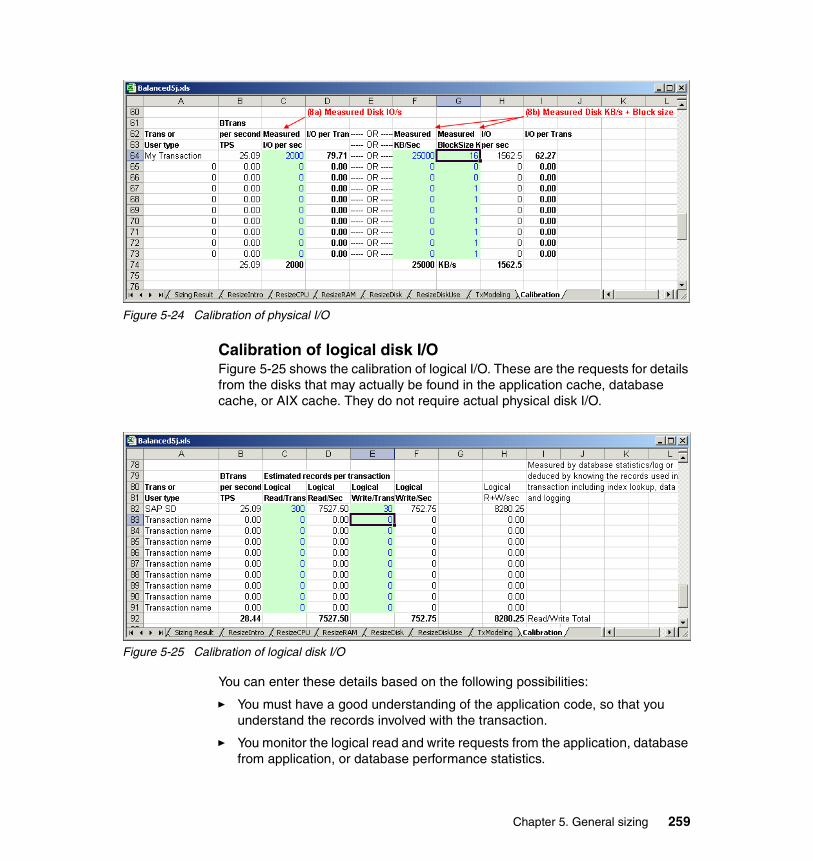
Figure 5-24 Calibration of physical I/O

Calibration of logical disk I/OFigure 5-25 shows the calibration of logical I/O. These are the requests for details from the disks that may actually be found in the application cache, database cache, or AIX cache. They do not require actual physical disk I/O.

Figure 5-25 Calibration of logical disk I/O

You can enter these details based on the following possibilities:

� You must have a good understanding of the application code, so that you understand the records involved with the transaction.

� You monitor the logical read and write requests from the application, database from application, or database performance statistics.


The logical I/O details are desired but optional. After the magic numbers are calculated, they can help to size more accurately.

5.4.12 Calibrating a new workload example: SAP, DB2, pSeries 650

From the SAP Web site, you can find benchmark details, for example, for a pSeries Model 650. See:

http://www.sap.com/benchmark/pdf/cert6002.pdf

Note the following details in this example:

� SAP Standard Application Sales and Distribution (SD) two-tier benchmark 4.6C

� Number of users: 900 SD

� Average dialog response time: 1.97 seconds

� Fully processed order line items/hour: 90,330

� Dialog steps/hour: 271,000

� SAPS: 4,520

� Database: RDBMS DB2 Universal Database (UDB) 7.2

� Operating System: AIX 5.1

� System: pSeries 650, 8-way SMP, POWER4 1.2 GHz, 1.5 MB L2 cache, 64 GB main memory, Certification 2002060 on 4 November 2002

You can use this information to add new applications to the Balanced System Guideline spreadsheet:

1. Start the Balanced System Guideline spreadsheet.2. Select the Calibration sheet.3. Add the following details:

– Peak Period: 3600 (the benchmark quote transactions per hour)

– Transaction Name: SAP SD2T Orders (this is a Sales and Distribution (SD) Two Tier (2T) benchmark and may not apply for other configurations)

– Users: 900

– Business Transaction in Total: 90330

Note: SAP is used here as an example application mainly because the SAP benchmarks are publicly available. Also the results documentation is concise and contains exactly the right level of detail.


http://www.sap.com/benchmark/pdf/cert6002.pdf

– Measured CPU Utilization Busy%: 97

– Test Machine rPerf: 15.5 from IBM Eserver pSeries Facts and Features, G320-9878, available at:

http://www.ibm.com/servers/eserver/pseries/hardware/factsfeatures.pdf

Figure 5-26 shows the CPU Seconds per Transaction of 0.599. This means that, on a one rPerf system, it takes over half a second of compute the time to perform one transaction. This is the magic number to use in the Sizing CPU and RAM sheet.

Figure 5-26 Calibration of CPU example

To confirm that this is correct for sizing applications, complete these steps:

1. Start the Balanced System Guideline spreadsheet.

2. Select the Sizing CPU sheet.

3. Add the following details:

– Select Clear to empty the fields and start from fresh.– Peak Period is 3600.– Target CPU Busy is 97.– Transaction Name is SAP SD2T orders.– Users is 900.– Business Transaction in Total is 90330/900. This field is per user.


http://www.ibm.com/servers/eserver/pseries/hardware/factsfeatures.pdf

– Safe CPU powerRequired should be around 15.5 (some rounding is likely).

4. Select the Sizing Disk sheet to remove any old disk numbers on this sheet.

a. Set Data Space Required to 1.

b. Click the Update button. This removes any large scale database requirement for this experiment.

5. Select the Sizing Results sheet. This sheet should indicate a system such as the pSeries 650 8-way (or the nearest current equivalent).

You can also use the dialog steps. If the sizing requester has these details instead of SD orders, you can use these for sizing. The differences from the Sales and Distribution Order transactions are:

� Transaction name: SAP SD2T dialog (reminds you of the measurement)� Business Transaction in Total: 271000

You now have the CPU Seconds per Transaction (dialog step) of ~0.2.

You can use the dialog transaction to size in the same way as the orders transaction.

Sizing sheet workload detailsThe preconfigured workload buttons and data found on the Sizing CPU and RAM sheet are described here. You can add more workloads simply if suitable benchmark performance and transaction data are available and used in the Calibration sheet.

� Clear: This empties most of the fields ready for further work to be used.

� TPC-C: This workload is based on the industry standard TPC-C benchmark. See 4.2.1, “TPC-C benchmark” on page 189, for more details. The benchmark has five transactions. You can use them individually or use an average of them all. The ratio of the individual transaction is shown in the transactions per user. The New Orders and Payment transactions are the bulk of the transactions.

Notice that the CPU power to run the transactions is surprisingly small. This is due to the fact the benchmark applications and database have been extremely well tuned over the lifetime of the benchmark.

Also the period is one minute since the TPC-C results are reported in minutes. Normally the spreadsheet calculates in seconds.

� Batch: Batch is an odd workload for several reasons:

– Batch workloads tend to require large amounts of CPU time and run “flat” for long periods. This is unlike OLTP type workloads which are smaller.


– The batch job is in the number of concurrent batch tasks running at one time, not by users.

– Batch jobs go through a large set of records and perform some function on them such as generating summary information or creating an invoice or report or transforming the data and storing it. To fit this workload into the sizing model, use the No. of Users field to represent the concurrent batch tasks. Also use the Transaction per user in period as the number of reports. By reports, we mean the number of tasks (summarizing, creating or reporting).

Use extra care with batch sizing since the size of a batch task varies considerably. To help you decide which of the light, moderate, or heavy workloads to use, check the logical I/O section near the bottom of the Sizing Disk sheet. In here, you find the number of records read to complete each batch transaction. Compare this with the actual batch job. If no information is available, this is impossible. If you guess, you need to highlight the assumed records read per batch transaction for the client to validate.

Many sites combine light batch tasks and OLTP workloads. You may have to copy the batch workload numbers to do both in one sizing. The alternative is to assume that the batch jobs use up the entire CPU on which it is running and four concurrent batch jobs take up four CPUs which must be added to the final requirement.

� 4GL: The fourth generation languages (4GL) were popular a few years ago. They are languages in which you write database-oriented applications. Most of the large database vendors developed their own language except for DB2. There are several database independent 4GL that work with the more popular databases. From the definition of how the screen appears, the database schema, and the code for particular tasks, the application is generated.

To decide which transaction to use, such as a batch workload, you can evaluate the logical I/O details or check the Transactions per User in Period column. The large transactions take the user much longer to fill in the details or study the resulting output (such as an online small report). Heavy complex users are only expected to perform four an hour. Light users perform 180 per hour. That is, every 20 seconds, they fill in some fields and save the data as though they were inputting basic client details or orders. 4GL applications are not as optimized as 3GL languages. It results in higher CPU use for the same task.

� Oracle Finance: This workload is based on an old Oracle Financial benchmark for a mix of three different user types. The ratios add up to 100, which you should use if you are using this to size relative to the benchmark. The user types are clearly defined in the benchmark description, and the names are helpful for you do determine which to use.


Journal Entry is the largest transaction. It involves adding a financial business transaction into the database. Account Inquiry is a simple lookup of a client’s basic data. Journal Inquiry finds the data added in the entry user type.

� Typical: If no application or database details are available, this is the workload to use. To decide which transaction to use, such as a batch workload, to evaluate the logical I/O details or check the Transactions per User in Period column. The large transactions take the user much longer to fill in the details or study the resulting output (such as an online small report). Heavy users are only expected to perform four an hour. Since 1000 reads are involved, they either extensively use the lookup fields in the database to add data or request a summary of many records in the database, such as the orders for the last three months. Light users perform 120 per hour. That is, every 30 seconds they fill in some fields on a simple screen form. Then they save the data or request the account details for a client while on the telephone to check some details.

� SAP: This workload is based on the SAP Sales and Distribution standard benchmark. There are two types of transaction here: the SAP dialog step or the orders processed. SAP is also highly configurable. Two tiers (database and application) are combined and there are three tier transactions (separate database server and application server). After you decide to use either transaction and two tier or three tier, set the others to blanks and fill in that one line.

� TSM: Tivoli Storage Manager (previously called ADSTAR Distributed Storage Manager (ADSM)) is the file backup and restore hierarchical storage software. Like batch, this is a hard to size because there are many statistics to gather before you size the system to run it. Use the detailed Tivoli Storage Manager spreadsheet helps to analyze all the client systems, their backup requirements, and rates. Then size the pSeries system to run a certain GB per hour backup to temporary disk space or directly to tape drives. You can also use the Tivoli Storage Manager database to store the filename, host, versions numbers, etc.

First in the Sizing Disk sheet add the Tivoli Storage Manager database size. Then use the No. of Users column to decide the number of concurrent client systems backing up data. For tape, this cannot be more than the number of tape drives. Use the Transaction per User per period column for the number of GB of data per hour per client.

Important: LAN speeds are important for backup. If you are backing up directly over the SAN from disk to tape and not via the pSeries at all, little CPU is used. Therefore, do not use these sizing numbers.


� App1, 2 and 3: This is for advanced users only to add your own application sizing data from benchmarks, prototype, or production performance data. You should change the matching fields in the hidden STATS sheet. If you have data for a well-known application, send it to the Balanced System Guideline team, so that others can use it and benefit from it.

5.5 Resizing existing systems for upgradesYou can upgrade existing systems and resize them for new workloads or better performance based on measured data and growth estimates. There is an introduction sheet followed by four interlinked sheets. Resizing data is input into the CPU, RAM and either the Disk or DiskUse sheets. The recommendations are on the same CPU, RAM, and Disk sheet.

5.5.1 AssumptionsThere are several assumptions when upgrading systems. These should come as no surprise to performance experts since upgrading system to increase performance or capacity planning is not too difficult.

� The system is reasonably well balanced. If the system is already drastically restrained by one resource (such as CPU, memory, adapters, disks), then upgrading the system generally still results in an unbalanced and unsatisfactory system.

� The system is reasonably well tuned. If the system has a bottleneck (for example, one very hot overworked disk), then upgrading other components may not effect performance at all.

� After the upgrade, new resources may require adjustments to the system. These may include spreading data across more disks, using extra adapters, making changes to applications to use more memory, or increasing parallelization with more CPUs.

� Suitably skilled technical specialists can extract the resizing information from the system. Or you can do it, but under their direction. Particularly useful is collecting Workload Manager statistics. Applications need to be suitably classified, Workload Manager ran in passive mode and Workload Manager statistics were collected. This allows for a detailed level of analyses to be completed for higher accuracy.

� The performance data is gathered during the peak period. Typically systems have a peak online period of an hour on one day of the week and at certain times of the year. For batch type workloads, this typically happens more often and at any time of day.


� The client has some expectations of the growth required on the system. This can be general growth by monitoring performance statistics or specific to CPU (for example, more transactions or users are expected) or disk space requirements due to planned storage of more data.

� If the system is totally overworked, (for example, the CPU utilization is above 98% for long periods or the response times are poor), then taking performance statistics can be misleading due to latent demand. You may have to upgrade everything to remove the bottleneck since it is difficult to determine the real cause. Studying the system when it is not so busy and comparing it to the overloaded state may help to identify the bottleneck.

Growth factorIn these sheets, no growth means a growth factor of one. If there is 50% growth, then this is a growth factor of 1.5. Triple the growth is a growth factor of three.

Simple and detailedOn the sheets, there are two levels of resizing:

� Simple: This level uses minimum facts about the system, but they are not accurate.

� Detailed: This level needs many more statistics (which are not difficult to determine with standard performance monitoring tools) and offers a much higher accuracy.

We highly recommend the detailed level.

5.5.2 ResizeCPU sheetThe ResizeCPU sheet allows the system and CPU data to be input at either a simple or detailed level and the new CPU power calculated based on growth. Workload Manager is ideal for gathering the detailed CPU use information since the application/class level is exactly what is required.

Figure 5-27 shows the basic data that you must enter for any resizing. The fields are explained here:

� Machine name: This is shown on each subsequent sheet. It is helpful if you print the sheets later.

� CPU Power Rating: This is vital and should contain the rPerf rating for the current system. These resize sheets are actually rating independent in that another rating number can be used since the sheets actually work out a factor by which the CPU power must grow.

� Physical Memory: This is the RAM of the current system.


Figure 5-27 ResizeCPU basic details

The following section explains the simple level. Then see “Detailed-level CPU resizing” on page 268.

Simple-level CPU resizingFigure 5-28 shows the ResizeCPU Simple Details section. It is assumed that basic monitoring of the system has taken place and that the peak period and CPU utilization are determined.

Figure 5-28 Simple level CPU resizing

In this example, the User CPU utilization, System (for example, AIX kernel) CPU utilization and growth factor are input. The growth factor is set to three for the User CPU time. The sheet estimates the new CPU requirement. Here, the


estimated CPU is more than three times the current CPU power rating because we plan to drop the average utilization to 75% for better peak period performance. This gives us a new CPU power rating of 50 rPerfs with a suitable safety margin of keeping the CPU 75% busy.

Detailed-level CPU resizingFor detailed level CPU resizing, more information is required about what your applications are consuming. Workload Management is absolutely ideal for this. After the application processes are classified, Workload Manager can be started in either passive or active mode and the CPU utilizations for each class are monitored with Workload Managerstat, svmon, or PTX.

See Figure 5-29 for an example of the CPU utilization broken down by Workload Manager class during the busiest hour. This type of break down means that you can apply the growth factor more intelligently to the correct application. You can then extract the average CPU use during the peak period from the same spreadsheet data and use it to fill in the Detailed Level section for CPU resizing.

Figure 5-29 CPU Utilization by Workload Manager Class

Figure 5-30 shows the ResizeCPU sheet’s detailed section. It is assumed that detailed monitoring of the system has taken place and that the peak period CPU utilization has been determined.

The “CPU Consumer” (the various applications, databases and the AIX operating system that use CPU power) names are only suggestions. You can change them if desired. These names are copied to the memory and disk sheets for consistency.

0102030405060708090

100

1 3 5 7 9 11 13 15 17 19 21 23 25 27

DefaultApp5App2WebRDBMSSystem


Figure 5-30 Detailed level CPU sizing

In our example, AIX (system), RDBMS, Web, and App5 classes are used as classes. The CPU utilization in the peak hour is monitored and entered into the fields. Only the RDBMS is expected to grow, so its growth factor is three and all the others equal one (meaning zero growth). The spreadsheet has calculated the new CPU power rating as 40. This includes the safety margin (75% CPU utilization). This is lower than the simple method calculations because only the RDBMS is growing and not the Web and App5 workload classes.

Note the RDBMS cache does not use any CPU. It only appears here so the lists are the same for CPU, memory and disks resizing sheets. The cache is important in the RAM sheet.

5.5.3 ResizeRAM sheetThis sheet allows the memory data to be input in simple or detailed levels and the new memory requirement calculated based on growth. Workload Manager is ideal for gathering detailed memory use information at the application/class level.


Simple-level memory resizingFigure 5-31 shows the ReSize Memory sheet’s simple section. It is assumed that basic monitoring of the system has taken place and the free memory is determined during the peak period.

Figure 5-31 Simple-level memory resizing

It is common for AIX systems, after a few hours of real work to show nearly zero free memory. This is due to the highly efficient file system cache management features of AIX using spare memory to reduce disk I/O by caching disk blocks. If there is free memory, then this calculation helps to determine a sensible memory increase. If not, then it has to be assumed that all memory was required and the growth factor must be applied to all memory.

Alternatively, you may explore the AIX numperm statistic. If a high percentage (over 80% for the default minperm and maxperm settings) on a system with more than 1 GB of memory, you can deduce that some free memory is available but it’s a little error prone.

There is an advanced technique to discover the real use of memory using an AIX command called rmss. You can use the rmss command to lock out and immediately free a small percent of memory. Then you can monitor how the memory freed is used. Going into the details of this technique is beyond the scope of this redbook.

Detailed-level memory resizingFigure 5-32 shows the ReSize Memory sheet’s detailed section. It is assumed that detailed monitoring of the system has taken place for the peak period and the memory utilization are determined. For detailed analysis, the memory used for each application must be determined accurately. Workload Management is absolutely ideal for this. After the application processes are classified, you can start Workload Manager in either passive of active mode. The memory utilizations for each class are then monitored using wlmstat, svmon, topas, or PTX.


In our example, the AIX (system), RDBMS, Web, and App5 classes are setup as Workload Manager classes. The memory utilization in the peak hour is monitored and entered into the fields. The RDBMS is expected to grow so its growth factor is three. Also the Web workload is expected to grow a little (1.5) and all others equal one (meaning zero growth). The spreadsheet shows that the new memory size is calculated as 3584 MBs. This is lower than the simple method calculations, but it is far more accurate.

The lower half of Figure 5-32 shows an alternative approach that you can use if the memory is not analyzed with Workload Manager. This involves guessing or measuring the sizes of processes for the different workloads.

The Example typical application sizes section allows you to estimate the size of the application and the number of copies running, usually one per user or batch task. You can fill in the Current MBs and the Number of Items fields and check them against the memory that is actually in the system. This is less accurate and more time consuming than the Workload Manager approach. However, it should still work and allow higher accuracy in predicting the required memory after you add the growth factor than in the simple method.

Figure 5-32 Detailed-level memory resizing


5.5.4 ResizeDisk sheetThe ResizeDisk sheet allows you to enter the disk data in the simple level only. You enter detailed data on the ResizeDiskUse sheet. This ResizeDisk sheet shows simple and detailed new disk requirement results based on growth.

Simple-level disk resizingFigure 5-33 shows the ResizeDisk sheet’s simple section. It is assumed that basic disk space allocation documentation of the system is available. The growth factor is used to calculate the extra disk space and the number of disks of various sizes that are required for the upgrade. This does not add a great deal of value, but it is here for completeness. For example, it allows you to document the many disks on the system and which groups of disks are to grow. It does not allow for hot disks that are overworked to be fixed (the detailed level does this).

The detailed disk analyses that follow are much more useful. The ResizeDiskUse sheet is used to supply the data and the detailed section is then automatically filled in.

Figure 5-33 Simple level disk resizing

5.5.5 ResizeDiskUse sheetThe ResizeDiskUse sheet allows the disk data to be input in the detailed level only. The new disk requirements are calculated and shown on the previous ResizeDisk sheet.


Detailed level disk resizingFigure 5-34 shows the ResizeDiskUse sheet or at least the part you are allowed to change. There are calculations that made below this section, but you should never change them.

For each disk in the system, the following information is documented:

� Size in GB: This is the size of the disks.

� Busy% Utilization: This is a measure of how busy the disk is during the peak period. This is used to factor in the automatic hot spot removal where extra disks are added to remove disk contention. This is described later.

� Workload: This is used to add the disks up and assign them to the right workload (for example, Workload Manager class). This allows automatic scaling to the correct set of disks. In this table, leave the cells blank except that you type 1 in the appropriate row and column to show in which workload (for example, class) each disk is located.

For example, in Figure 5-34, hdisk1 contains the AIX operating system, so we type 1 in cell E8. The RDBMS data is spread across hdisk2, hdisk3, and hdisk4. Therefore, we type 1 into F9, G9, and H9.

Figure 5-34 Detailed level disk resizing

This sort of data is normally available from a well-organized systems administrator plus the regular performance monitoring tools such as iostat, filemon, or PTX.


This spreadsheet has a limited number of disks that it can handle. This can be extended by any someone who is reasonably proficient at spreadsheets or you can group disks together.

For example, you have 64 disks made up of eight packs of eight disks each and a size of 36 GB. Each pack is used evenly in just one workload. In this case, you can combine the eight disks by making the size 36 x 8 = 288 GB. Then fill in the other fields as before instead of the individual disks.

Under the details in Figure 5-34 are the calculations to work out the hot disk removal and the summary details that are displayed on the previous ResizeDisks sheet. This means if this ResizeDiskUse sheet is completed, there is no work for the detailed analyses except to add the growth factor.

Detailed disks summaryFigure 5-35 shows the summary details that are taken from the ResizeDiskUse sheet’s data. Most of the details are taken from that analysis. Only the growth factor has to be added.

Figure 5-35 ResizeDiskUse summary details

Notice the difference between the disk size and the sizes after hot spot removal. This uses the simple rules of thumb to add disks to spread out the disk I/O across more spindles as follows:

� 80% to 100% Busy: Add this many more disks since this disk is extremely busy.

� 60% to 80% Busy: Add two more disks since this disk is very busy.


� 40% to 60% Busy: Add one more disk since this disk is busy.

� 0 to 40% Busy: Add no more disks since this disk is not that busy.

This should make the system perform better and eliminate bottlenecks. The growth factor is then added to give the final sizes. Finally, the difference is determined and the number of disks at various sizes is calculated. In the example, fifteen 72 GB disks are needed but twenty-nine 36 GB disks is better. More spindles means faster I/O rates.

The person who is performing the sizing needs to make a judgement on which disks and their sizes to recommend from the list.

5.5.6 Modeling to add new workloadsTo perform modeling for new workloads, use the TxModeling sheet. The following sections explain this sheet as well as the Transaction Modeling sheet.

TxModeling sheetThe TxModeling sheet is used to determine the business transaction rates and database transaction rates from business requirements. Use this spreadsheet if you have general information about user numbers and their workload and need to translate them to transaction rates.

This sheet is normally used by someone who is:

� Planning a benchmark� Deciding a mix of transactions for a benchmark� Converting transaction rates for longer periods like per day, month or year into

rates more appropriate for sizing

Transaction rate convertingFigure 5-36 shows a simple converter between transaction rates of different time periods. The rest of the Balanced System Guideline spreadsheet tends to encourage input of transaction rates for time periods of an hour (3600 seconds) and seconds. The actual calculations are always done in seconds, for example, transaction per second. This avoids large mistakes and simplifies things. Many sizing or resizing requests supply data in other time periods and must be converted. This is error prone, so this sheet reduces the likelihood of errors.


Figure 5-36 Transaction modeling converter

Also, the times at which the data is provided in terms of transaction per day (or week, month, year) is not helpful and misleading. Most daily transactions do not have 24 hours to be completed but a working day (7 to 9 hours). Even then, there is likely to be a peak period. The lower half of this sheet can help you estimate a realistic peak hours transaction rate from data for a longer period.

Transaction Modeling sheetFigure 5-37 shows the other section of the Transaction Modeling sheet which is used to work from business transactions. Such transactions include adding a sales record or updating a client record, user numbers and transaction rates into such database transactions as select, update, delete and insert, to determine the overall database tractions rate.

In this example, 1000 users are doing three different transactions at different rates. By knowing the number of database interactions for each transaction, we can determine that this system is doing around 142 database operations per second which is easily within the capability of the pSeries range.

The very small transaction can be found in the TPC-C workload. This can give you a feel of the transaction rates that are possible. Note that TPC-C sized transactions are rare in real production workloads.


Figure 5-37 Transaction modeling business to database transactions

5.6 Balanced System Guideline and sizing levelsThis section reviews the inputs required for each level of sizing.

5.6.1 Sizing for Level 2: ‘Ball park’ or rough estimatesFor sizing at Level 2, use the following input fields in the Sizing CPU and RAM and Sizing Disk sheets only:

� Application type� Number of users� Raw data or disk size

Then following recommendations are on the Sizing Results sheet:

� CPU requirements � Memory� Disks number and type� pSeries model recommended


5.6.2 RDBMS server sizer for level 3: Consider opinionFor sizing at Level 3, use the input fields in the Sizing CPU and RAM and Sizing Disk sheets:

� Application type� Number of users� Raw data or disk size� Transaction mix� Users/transaction rates� Choice of disk type� Read and writes per transaction

The output is the same as Sizing for Level 2: ‘Ball park’ or rough estimates, but is now based on your more accurate figures rather than the defaults.

5.6.3 Sizing for Level 4: Sizing from measured dataYou must measure the transactions for their CPU use, memory use, and generated disk I/O (at least physical disk I/O). You can do this from a production system, prototype, or suitable benchmark. Also a more detailed investigation into the real users transactions per hour rates (rather than guesses) can increase accuracy.

5.7 Business intelligence sizingThis is a complex area for sizing. It is due to the broad range of applications, many application vendors, the underlying database designs, query types, and platform types (SMP or parallel clusters) used to implement BI. This explains the other names that this type of workload also goes by, for example, Data Warehouse, Decisions Support, Data Mining, OLAP, ROLAP, Data repository. This reflects the differences in approach taken by vendors. Also this area requires high system resources, typically three times the I/O and CPU compared to a OLTP system.

Fortunately, the pSeries is an excellent architecture for BI due to the range scaling by a factor of 45 and then higher still with clustering in extreme cases. These superior balanced systems, with respect too all models, have the memory and I/O capabilities to feed the processors needs.

Important: It is easy to confuse level 2 and 3 sizing. Think about what you have taken as defaults and what you know to be accurate.


No account is taken here of the database vendor, version, or database disk or disks and topology. The estimates shown here are generally safe for small or medium systems. In larger configurations, there is the potential for larger errors.

5.7.1 Business intelligence golden rulesThere are three workloads to consider. The following rules of thumb apply to a balanced system and to size from the workload:

� Online access for users submitting queries:

– 45 GB of raw data per rPerf– 2 GB of memory per rPerf– I/O bandwidth for response time critical queries:

• 38 MB per second for complex queries• 14 MB per second for medium queries• 8 MB per second for simple queries

� ETL (extract, transform and load) to add data to the database:

– 3 to 5 GB per hour per rPerf

� Aggregation (generating data cubes, etc.):

– No rules of thumb are available due to the variety of source data, indexes, and applications

The ETL workload is often higher than the online work.

Choose small disks and many of them since high I/O throughput is mandatory.

5.7.2 Business intelligence sizing approachesFrom the previous two approaches to sizing, you can use the following information:

� From the data volume, the CPU and memory requirements can be estimated.

� From the queries, the I/O rates can be estimated, and the disk subsystem can be decided to achieve these rates.

Notes:

� The BI systems have a much higher raw data to disk ratio.

� These numbers are used in the Balanced System Guideline spreadsheet for balanced systems.


The complex, medium, and simple need more explanation. Most BI system have a wide mixture of queries. They range from those that can be quickly answered in seconds from summary tables to those that require plowing through base data looking for completely new trends. To work with these mixtures, three queries are defined (Table 5-1) and used in different proportions in three workloads.

Table 5-1 Queries

Table 5-2 defines the BI “standard” workloads.

Table 5-2 BI standard workloads

If you don’t have any further information, use the rule of thumb that a user submits 10 queries each hour.

5.7.3 Business intelligence sample configurationsThe following list outlines sample configurations and includes comments for a range of systems:

� pSeries 615 1.2 GHz 2-way

– Worth considering for small BI or to prototype large solutions.– Raw data is less than 150 GB.– Users are less than 75.– 8 GB memory is used.– You can choose CPU speed for best price/performance option.– Requires roughly 16 disks, so use internal and a drawer of SCSI or

FAStT200.


– Raw data is less than 350 GB.– 16 GB memory is used.– Is a good match for entry-level FAStT such as FAStT600.

Query Explanation

Simple Uses indexes and summary tables

Medium Uses reference table data via indexes

Complex Uses minimum indexes and involves full table scans

BI workload Simple query Medium query Complex query

Light 90% 7% 3%

Medium 70% 20% 10%

Heavy 50% 30% 20%


– Is good for clustering with parallel DB2.– Is good for a two or three node Oracle RAC.– Use two Fibre Channel adapters for disk access (and RAS).– If clustering, don’t forget to add one or two Gb Ethernet network adapters.


– Raw data is between 350 GB and 800 GB.– 32 GB memory (possibly 16 GB, if using 1.2 GHz CPUs) is used.– Is a good match for midrange FAStT such FAStT700.– Is good for SMP configurations to avoid clustering complexity.– Add Gigabit Ethernet network adapters.– Use four to six Fibre Channel adapters for disk access.– If clustered, don’t forget to add two Gb Ethernet adapters.

� Cluster of pSeries 655 1.7 GHz 4-way

– Raw data is greater than 3000 GB.

– 24 GB memory is optimal, but you can go to 16 or 32 GB in practice.

– Is good match for midrange FAStT such as FAStT700.

– Is a good alternative to pSeries 670 and 690 for 1000 GB or more by clustering.

– Add one switch adapter or two Gb Ethernet network adapters.

– Add four Fibre Channel adapters for disk access.

– Two pSeries 655s that share a remote I/O drawer, which makes a good building block.

– Due to the pSeries 655 rack size and costs, the pSeries 655 makes particularly good sense in a cluster of six or more nodes.

– Optionally you can add other pSeries 655 nodes to the BI cluster for specific BI-related functions such as ETL during online day, user-long running queries, and access to data cubes or NFS.


– Raw data is between 1000 GB and 3000 GB.– 128 GB memory is used.– Is a good match for one or more ESS or top-end FAStT (FAStT900).– Use two or more Gb Ethernet network adapters.– Use 24 FC adapters for disk access.– Is a good choice for Oracle since it avoids RAC complications.– Is ideal for mixed environments with other LPARs running along side since

it adds flexibility in CPU use at peak times.


� Clustered pSeries 690

– Raw data is up to 5000 GB.

– Add one switch adapter. This requires multiple LPARs for bandwidth and a cluster of smaller systems, which is a less expensive option. Or add eight Gb Ethernet network adapters each.

In a clustered configuration, you get roughly the same price/performance from:

� Four 4-way pSeries 630s � Two 8-way pSeries 650s� Three 4-way pSeries 655s

When clustering, you should also expect to use:

� Cluster System Management (CSM) to reduce complexity and manpower for systems administration

� General Parallel File System (GPFS) to create parallel access to the files and for RAS

5.8 Disk and stripe sizingThis section looks at the issues surrounding disk sizing and disk striping.

5.8.1 Disk sizingDisk sizing consists of more than buying enough disks to hold the data. You must also assure that performance and availability goals are met. Trade-offs exist between performance, availability, and cost. For example, RAID-5 implementations provide a relatively lower cost, but reduced performance. A single write from the application generates four I/Os on a RAID array. Mirroring, or RAID 1, provides availability and high performance but requires buying twice as many disks.

Other factors are important. Additional memory (and clever programming) can reduce I/O. Some say that the best I/O is no I/O. Oracle uses the SGA, and DB2 uses a buffer pool to reduce I/O, while AIX uses extra memory to cache file system I/O. The AIX device drivers and disk drives also use advanced techniques to improve disk performance.

Keep in mind that a bottleneck is not necessarily bad. While you will always have bottlenecks, and removing one creates another, removing a bottleneck improves performance. Other factors provide additional cushion. For example, increasing memory reduces the I/O load. Also, you may experience Small Computer System


Interface (SCSI) bottlenecks that don’t exist with SSA or Fibre Channel. Newer disks may have better speeds and feeds.

5.8.2 Stripe sizingThe best stripe size is difficult to determine as long as trade-offs exist. There are two appropriate ways to evaluate this:

� Use a queuing theory, such as a BEST1 analysis� Test your application with various stripe sizes

Both options require considerable time, money, and effort. Here we try to provide some insight into the issues.

AIX has a read-ahead feature so that when a program reads sequential pages of a file, the virtual memory manager schedules additional sequential reads of the file. This feature, along with a small stripe size, causes (for the case of a single user) reads to occur simultaneously over several disks. This increases the throughput to several times that of a single disk. With many users, however, smaller stripe sizes can cause performance to be worse, which we explain later. We also make assumptions about disk performance that vary depending upon disk type, but that are good enough for the purposes of examining stripe size.

Disks have several limiting factors. Seek (the time to move the head to the appropriate track) and latency (the time to rotate the disk to the sector we want to read) are commonly referenced and measured in milliseconds (ms). Let’s assume a seek + latency time of 12ms. The media or data rate (how fast we read/write data given that we don’t have to worry about seek and latency) is another limiting factor. This rate is measured in MB per second (MB/s), approximately the same as KB per millisecond (KB/ms). We assume a data rate of 8 MB/s or 8 KB/ms. A less commonly known limit is the maximum number of I/O per second. That is, given a particular disk and assuming a specific mix of random or sequential and specific I/O size, a disk can perform only so many I/Os. If all I/O to a disk is random, then a disk can only perform 80 I/O per second (assuming seek + latency of 12 ms and reads of 4 KB). Assuming all sequential I/O, with I/O sizes of 4 KB, then a disk can perform 2000 I/O per second. Obviously we want to avoid moving the head.

How can smaller stripe sizes and many users cause performance to get worse? Consider a simple two-user and two-disk scenario with each user performing a 64 KB I/O when using a 32 KB stripe size (assume sequential I/O and that the I/O occurs on two stripes only). In this case, each user has to perform two start I/Os, one to each disk. This causes two seeks per disk for a total of four start I/O. For two users using 8 MB stripe sizes, we either get two seeks on one disk or one seek per disk on two disks, for a total of two start I/O. In either case, with 8 MB


stripe sizes, we have one-half the start I/O operations. After a disk’s start I/O capacity is exceeded, performance suffers. To summarize this concept:

� Start I/Os increase proportionally with the number of I/Os that overlap stripe boundaries.

� Smaller stripes increase the probability that an I/O overlaps stripe boundaries.

The reality is that there are many users with many disks and a mix of I/O sizes and types. Therefore, the queuing theory, statistical modeling, or actual testing are the only ways to determine the optimum stripe size.

The key point for efficient use of the disk subsystem is the even distribution of the I/O across as many spindles as possible. Assuming your I/O patterns are random across your logical volume structures (or data files in Oracle terminology), any stripe size that spreads the logical volumes across the disks is evenly distributed the I/O among the disks. This indicates that a wide range of stripe sizes may be equivalent and optimal for a given environment, that is, stripes greater than the average I/O size but small enough to spread the data across the disks.

Oracle provides further guidance in setting up logical volumes. For example, Oracle recommends putting data tables and indices on different disks. This assures that the index lookup and the data read occur on different disks, resulting in better response time. This spreads data files across one set of disks and indices across another. Since the I/O to the indices typically uses more bytes than the data, we must often put the indices on more disks than physically necessary.

5.9 pSeries 670 and 690 RIO-2 I/O Sizing ToolThe pSeries 670 and 690 RIO-2 I/O Sizing Tool is a spreadsheet. It is designed to assist in the planning and analysis of 7040-61D configurations. 7040-61D is product number of the I/O drawer for pSeries 670 and 690. For ordering purposes, the difference between them is the feature code of the configured I/O planar:

� RIO drawer uses the FC 6563, I/O Drawer PCI Planar, 10 slots, two Integrated Ultra3 SCSI Ports.

� RIO-2 drawer is configured with the FC 6571, I/O Drawer PCI-X Planar, 10 slots, two Integrated Ultra3 SCSI Ports.

This easy-to-use spreadsheet allows users to input the quantity of each type of I/O adapter required in the system configuration. The tool analyzes the input and provides the user with the number of drawers, MCMs, and loop adapter cards that are required to support the proposed configuration. In addition, the tool


shows the estimated total bandwidth required by the adapter selections. It also provides drawer recommendations that are designed to support this adapter bandwidth.

Adapter descriptive data, notes, messages, and warnings are also provided to assist the user to develop properly designed I/O drawer configurations for RIO-2 solutions.

5.9.1 Notes and assumptionsConsider the following points when using the pSeries 670 and 690 RIO-2 I/O Sizing Tool:

� Adapter bandwidth and performance information in this tool are only an estimate. Actual performance depends on many factors including workload, protocol, tuning, contention, and the performance of other attached devices.

� Peak adapter bandwidth is generally not achieved. Therefore, the tool allows drawer bandwidth to be exceeded by 20% before an additional drawer is added to the drawers count.

� This tool only supports RIO-2 configurations using planar FC 6571. For configurations using planar FC 6563, use Version 2 of the tool.

� Only full drawer, non-mixed planar configurations are considered. However, half-drawer (single planar) and mixed-planar configurations are allowed.

� Limits specified for drawers, adapters, slots, etc. are based upon pSeries 670 and 690 capabilities announced May 2003.

� This tool does not provide I/O balancing analysis. Certain workloads may benefit from having adapters distributed over multiple host buses and I/O planars. Adapter placement rules may provide some I/O balancing, but additional analysis may be necessary for critical workloads.

� Additional I/O drawers over the minimum recommended may indeed be desirable to provide a required performance buffer, growth capacity, or I/O balancing capability.

� Except where noted, the tool assumes that all adapters are used (no standby/spare adapters) and that adapter limits are established with the same assumptions.

Attention: This spreadsheet is provided to IBM and IBM Business Partners to assist with pSeries 670 and 690 installation planning. You can use it for planning purposes only. It is being provided by IBM on an “as-is” basis. IBM makes no representations or warranties regarding this tool and does not provide any guarantee or assurance that the use of this tool will result in a successful client installation.


� Configuration rules applied by this tool are a subset of the pSeries 690 configurator rules. Results may vary.

The following sections explain the sheets in the pSeries 670 and 690 RIO-2 I/O Sizing Tool and how to use them.

5.9.2 Readme sheetWhen you start the pSeries 670 and 690 RIO-2 I/O Sizing Tool, you see the Readme sheet as shown in Figure 5-38. This sheet contains an introduction to this tool, version, instructions, notes, and assumption.

Figure 5-38 RIO-2 I/O Sizing Tool: Readme sheet

5.9.3 Adapters sheetFigure 5-39 shows an example of the adapter planning worksheet. It contains the list of adapters that can be used for RIO-2 I/O drawer, descriptions, characteristics (such as 64-bit and limitations) and the input columns that you can modify. If you specify the number of adapters in this sheet, then results are

Important: This tool can change without any notice to include the latest information. Check for updated versions regularly.


generated automatically and shown in the Results sheet (see Figure 5-41 on page 289).

The Adapter sheet includes several fields to configure adapters for the 7040-61D I/O drawer. This sheet also groups the adapters by their characteristics, such as Fibre Channel, graphics, and network. This sheet contains the most important information related to configuration, such as feature code, adapter description, and several configuration limits, so the user can identify the adapters easily.

Figure 5-39 RIO-2 I/O Sizing Tool: Adapter sheet

The fields in this sheet are:

� Enter Quantity: This is the only column where input is required. In this column, you type the number of the adapters that you need.

The last row of this sheet shows the total number of the configured adapters as shown in Figure 5-40.

� Feature Code: This column displays the feature code of the adapter.

� Adapter Description: This column describes the adapter.

� 64-Bit: If this column is marked with X, it means that the adapter’s bus width is 64-bit.

� Peak Bandwidth: This is the peak time bandwidth of the adapter.

� Total Bandwidth: This specifies the sum that results from multiplying the value in the Enter Quantity field by the value in the Peak Bandwidth field. It indicates the estimated total bandwidth required by the adapter selection.


The last row of the sheet shows the sum of the estimated total bandwidth required by the adapter selections. This number is used to decide the drawer recommendations as shown in Figure 5-40.

Figure 5-40 RIO-2 I/O Sizing Tool: Adapter sheet

� #6571 Planar Limit: This defines how many specified adapters of one type can be physically plugged into a planar (FC 6571).

� Drawer Limit: This defines how many specified adapters of one type can be physically plugged in to a drawer.

� Multiple Drawers Triggered: If the number of adapters exceeds the drawer limit, it is automatically turned on as YES to let user know it easily.

� p670 System Limit: This defines how many specified adapters of one type can be physically plugged in to a pSeries 670.

� p690 System Limit: This defines how many specified adapters of one type can be physically plugged in to a pSeries 690.

� LPAR limit p670/p690: This is the informative column for LPAR configuration limit. This defines the maximum number of adapters of on type per LPAR. This value doesn’t make any effect to the result.

� p670 Combined limit: The pSeries 670 can be configured with mixed. The mixed I/O means that one of the I/O planars is an RIO planar (FC 6563), and the other one is an RIO-2 planar (FC 6571). This is the informative column for this combined configuration limit. This value doesn’t affect the result.

� p690 Combined limit: The pSeries 690 can be configured with mixed. This is the informative column for the pSeries 690 combined configuration limit. This value doesn’t affect the result.


� EEH: This is the abbreviation of extended error handling. If this column is marked as Y, the adapter has the EEH capabilities built in to their device driver.

� Notes: This shows some considerations and other information for the adapter configuration.

5.9.4 Results sheetThis sheet displays a suitable I/O configuration for selected adapters. These numbers are based on the input into the Adapter sheet. Figure 5-41 shows an example of this sheet.

Figure 5-41 RIO-2 I/O Sizing Tool: Results sheet

The fields of the Results sheet are:

� Total Bandwidth: This column shows the sum of the estimated total bandwidth required by the adapter selections. It’s based on the Adapter sheet.

� Total Slots Required: This column shows the total number of the required adapters. It’s based on the Adapter sheet.


� Single Loop Configurations with #6571 (RIO-2) PCI-X planars: This column shows the number of minimum drawers to support selected adapters for single loop configuration planar.

� Performance Optimized Double Loop Configurations with #6571 PCI-X Planars: This column shows the number of minimum drawers to support selected adapters for a double-loop configuration planar.

� Analysis: You can use this column for the I/O drawer configuration. It gives you the minimum number of drawers, MCM, and FC 6419 Loop Attachment Adapters for various configurations.

It also provides the total drawer bandwidth utilization percent based on duplexed I/O bandwidth.

� Errors/warnings: Error or warning messages are displayed in bottom part of this sheet. They indicate that something is wrong with your configuration. You can find more information about the errors in the p670/p690 Errors sheet.

Note: The communication from the Central Electronics Complex (CEC) to the I/O drawers is done over the remote I/O link. This link uses loop interconnect technology to provide redundant paths to I/O drawers. There are two modes of loop operation:

� Single-loop mode: The two I/O planars of an I/O drawer belongs to the same loop, which is connected to one pair of ports of an I/O book.

� Dual-loop mode: Each I/O planar of an I/O drawer belongs to one loop, which connects to one pair of ports of an I/O book. The two loops connected to one I/O drawer must connect to pairs of ports in the same IO book.

The I/O books plug into the GX slots in the CEC backplane and provide the remote I/O (RIO) ports. The RIO ports are used to connect I/O drawers to the GX bus. Each I/O book contains a base card, a riser, and a daughter card. They are physically packaged using book packaging technology.

RIO-2 books support both single-mode and dual mode loops, while RIO books only support single-mode loops. Because of the cabling rule for I/O book port pairs and I/O loop pairs (see the IBM Eserver pSeries 670 and pSeries 690 System Handbook, SG24-7040), the maximum number of I/O drawers and the maximum data rate that can be reached for each of the cabling patterns are different.


5.9.5 p670/p690 errors sheetFigure 5-42 shows an example of a warning message in the p670/p690 Errors sheet. In this example, 19 adapters are selected. This number of adapters can be accommodated in one drawer, so the Results sheet’s minimum recommended 040-61D I/O drawers display a 1. Total required bandwidth to support selected adapters exceeds 80% of the one drawer bandwidth utilization. In this case, you should add one more adapter for the performance.

This sheet explains the reason that triggered the error/warning messages. You can correct error messages in the Adapter sheet according to the message. For warnings, consider the information in your I/O drawer configuration.

Figure 5-42 RIO-2 I/O Sizing Tool: Errors sheet

5.9.6 RIO-2 loops sheetThis sheet displays the relationship between the MCM and loop attachment adapters as shown in Figure 5-43.

The components involved in the creation of a loop are:

� RIO books (located in the CEC): The primary and secondary books have, respectively, two or four pairs of RIO ports.

� RIO planars (located in the I/O drawer): All drawers have two pairs of ports, one on each planar.

� RIO cables: Cables are different to plug into an RIO port or an RIO-2 port.

The I/O books plug into the GX slots in the CEC backplane and provide the Remote I/O (RIO) ports. The RIO ports are used to connect I/O drawers to the GX bus.


Figure 5-43 RIO-2 I/O Sizing Tool: RIO-2 Loops sheet

Two types of I/O books are available: primary I/O book (FC 6418) and secondary I/O book (FC 6419). The primary I/O book is mandatory in all pSeries 670 and pSeries 690. There must be exactly one per system. The secondary I/O books are optional. Their number depends on the requirements for external IO drawer attachments. A pSeries 670 can contain at most one secondary I/O book. A pSeries 690 can contain up to three secondary I/O books.

This sheet has a table that indicates the number of available I/O loops for each combination of MCMs versus Loop Attachment Adapters (FC 6419) that are available.

5.10 Review and summaryAfter the person who is performing the sizing determines the hardware requirements, the system or systems that are to provide the resources must be selected. The hardware requirements are stated in terms of:

� CPU: Estimated CPU power rating� RAM: Estimated memory size in GBs� Disk storage: Size and estimated number of the disks

The building block and details of the configuration must be determined so that a configuration can be created in the IBM eConfig tool for ordering and pricing. Therefore, you need the following details:

� The pSeries model� The number of CPUs� CPU type (GHz rating and other options)� The memory type (SIMMS or books size in terms of MB or GB)� Number of memory SIMMS or books


� The number of internal disks and their size� For external disks:

– The number of disk adapters and their type– The disk storage subsystem type– The number of disks– The number of drawers/tower in which they are housed

� The number and type of network adapters� Other internal units such as:

– Tape drives– CD-ROMs– Power supplies– Redundant fans, blowers, etc.

If this solution is three tiered or has several independent inter-working components, then there is a hardware requirement for each. The next phase is to consider the building blocks that make up the system.

Fortunately, the pSeries range is extremely flexible, which means someone has to decide. Often it is understood based on the sizing request. For example, the request may state that they want a single large system with logical partitions (for maximum flexibility) or for cost reasons and the application’s natural fit, a cluster of smaller systems is most appropriate. If there is no such guidance, then the person doing the sizing has to make the decision, discuss this with the requester, or provide multiple solutions and options for the client to decide.



Chapter 6. Application-specific sizing

This chapter provides application-specific sizing information for applications from IBM (DB2, Lotus, Tivoli, WebSphere) and independent software vendor (ISV) software families, that are available on the pSeries platform. The information is structured around key criteria numbers that are needed for accurate sizing, available tools for sizing, and the IBM sizing process. Some sizing estimations are also included.

The chapter also provides information about IBM Eserver Sizing Guides. These guides provide sizing recommendations for servers (including pSeries) that run one or more workloads associated with e-business and collaboration.

6

Important: For sizing assistance, send e-mail to mailto://[email protected]. We highly recommend that you use the sizing and planning questionnaires that are mentioned in this chapter.


mailto://[email protected]

6.1 IBM applicationsThe following sections outline sizing information regarding IBM applications that are available on the pSeries platform.

6.1.1 DB2DB2 is the IBM database software. It provides the foundation for information on demand. The following sections present sizing information for applications that are part of the IBM DB2 family.

DB2 Universal Database DB2 Universal Database (UDB) is a multimedia, Web-ready, relational database management system. The information regarding the DB2 UDB sizing for Data Warehouse and online transaction processing (OLTP) environments is outlined in the following topics.

DB2 UDB Data WarehouseThe database server sizing for a data warehouse environment is a complex process. Use the following key criteria for this sizing process:

� Query types:

– Simple %: A simple query is an indexed query. It typically retrieves 50K of data. The response time goal is less than 0.1 minute.

– Medium %: A medium query uses some indexes, table scans, multi-way joins, or all three, and some ORDER BY. Typical query reads from disk 0.1% of the data. The response time goal is about 5 minutes.

– Large and Complex %: Large and complex query uses full table scans, multi-way joins, and a lot of ORDER BY. Each query reads from disk a significant amount (20%) of data. They are very input/output (I/O) intensive. The response time goal is about 120 minutes.

� Extract, transform, and load (ETL)

– Is it heavier than the query work load?– Is it done along with the queries?– If you answered “No” to each of theses questions, then ask:

• What is the input data volume?• What transform is required (input row length, output row length)?• How many secondary indexes should you build during LOAD?• How many aggregates are there?


� System information

– Read-only?– 7x24 system?

� Type of configuration needed

– Standalone (for example, UDB ESE) – Cluster (for example, UDB ESE with partitioning feature)

The recommendation may be different. For a large multiprocessor system recommendation, we recommend UDB ESE with the partitioning feature.

� Peak query per hour

This is the query rate for your business intelligence (BI) system. This is not the number of Structured Query Language (SQL) statements.

� How many reads or writes per query?

� Users per system (consider future growth)

– Number of total user population – Number of users in a one-hour period– Number of queries per active user per hour

� Data and database (consider future growth)

Examine the raw data size and percentage active, or database size and percentage active. Raw data size is the size of the flat file or files before they are loaded into the database. Use this if you do not have an existing database system. Use the database size if you have an existing DB2 database system on pSeries and you anticipate growth. The database size includes data, indexes, temporary space, and database overhead in the database.

Percentage active means the percentage of data that is searched by queries. For example, many data warehouses contain historical data of three to five years. However, only the data in the next 12 months is used by queries.

� Disk requirement

– RAID type – Other storage system requirements

� Desired contingency (headroom) in percentage

At least 15% is recommended.

You can use this information in the data warehouse sizing process. Contact your IBM Technical Sales Support representative to assist you in sizing a BI data warehouse. They have access to a BI sizing tool. Your IBM representative can obtain the DB2 UDB Data Warehouse Sizing and Planning Questionnaire to assist with sizing.

Chapter 6. Application-specific sizing 297

DB2 UDB OLTPThe key criteria to use for the DB2 UDB OLTP sizing process are:

� Transaction complexity

– What is your business?

• Typical Complex Configurable Financial Package• Typical Simple Application (in C or COBOL) Transactions• Typical PC-based graphical user interface (GUI) forms application

written in 4 GL• TPC-C (OLTP benchmark transactions)

– Transaction types

• Simple % • Medium % • Large and Complex %

� Batch workload (for example, typical batch reports)

– Is it heavier than the transaction work load? – Is it done along with the transactions? – If you answered No to each of these questions, then concerning OLTP

(typical batch reports) answer:

• How many jobs are there in a one-hour period?• How many reports are there per job per hour?• What types of reports are there?

- Batch Heavy Complex %- Batch Moderate Heavy % - Batch Moderate % - Batch Moderate Light % - Batch Light %

� System information

– Read-only?– 7x24 system?

� Type of configuration needed

– Non-cluster db server (for example, UDB ESE)– Cluster db server (for example, UDB ESE with partitioning feature)

The recommendation may be different. For a large multiprocessor system recommendation, we recommend UDB ESE with the partitioning feature.

� Peak Transaction Per Hour

This is the transaction rate for your OLTP system. It is not the number of SQL statements.


� How many reads or writes per transaction?

� Users per system (consider future growth)

– Number of total user population – Number of users in one-hour period

� Data and database (consider future growth)

– Raw data size and percentage active, or database size and percentage active

Raw data size is the size of the flat file or files before you load them into the database. Use this if you do not have an existing database system. Use database size if you have an existing DB2 database system on pSeries and you anticipate growth. Database size includes data, indexes, temporary space, and database overhead in the database.

Percentage active means the percentage of data which is searched by transactions. In the case of a normal OLTP system, percentage active is generally higher than 80%.

– Percentage of image files and sound files and large text files of the raw data

– More than one secondary index per table?

– Does the database consist of mainly small tables or just a few of big tables?

� Disk requirement

– RAID type – Other storage system requirements

� Desired contingency (headroom) in percentage

At least 15% is recommended.

You can use this information in the OLTP sizing process using the Balanced System Guideline spreadsheet described in 5.4, “The Balanced System Guideline details” on page 225. You can obtain a DB2 UDB OLTP Sizing and Planning Questionnaire from your IBM Technical Sales Specialist for assistance in sizing.

DB2 Content ManagerDB2 Content Manager provides a foundation for managing, accessing, and integrating critical business information on demand. It lets you integrate all forms of content–document, Web, image, rich media–across diverse business processes and applications, including Siebel, PeopleSoft, and SAP.


On the sizing process for DB2 Content Manager, we mention that:

� For calculating the usage of the servers, the two biggest factors in your workload description are the number of clients and the number of actions each client performs in an hour.

� For calculating the size of the databases and the amount of disk or IBM Tivoli Storage Manager storage required, the two biggest factors are the number of documents and the average document size.

To size a DB2 Content Manager system, information regarding the system and the client workload are necessary.

To calculate an estimate of yearly volumes from questions about daily or hourly workload and basic system information, consider:

� How many hours daily will you load documents into the system?

� How many daily ad-hoc searches will the users perform?

� How many business days per year will the system be available (typically 260)?

� For how many years must the system has to be sized?

The stress on the system is calculated by multiplying the number of clients attached to the system by the number of actions that they perform during the peak workload hour. With this information, the number of searches, retrieves, and processing actions that hit the mid tier, library server, and resource manager during the peak hour are calculated.

In general, after each action, a user wants to review the response. A user who performs more than 30 actions per hour (one every two minutes) is a heavy user.

Consider this client workload information (Web and local area network (LAN)):

� How many Web clients and LAN clients do you expect to be logged on during your heaviest use peak hour?

� How many times during the peak hour do you expect a client to:

– Conduct a search?– Retrieve a document?– Update a document or folder (re-index, modify an annotation)?– View individual pages through the Web?– Open a folder?– Add an item to a folder?– Start or advance a document or folder through a process?

Items (documents, folders, items and resource items) are assigned an item type when they are stored in the system. From the item type, an item has user


attributes and a content migration policy defined for it. For each item type, an item description with the following elements is necessary:

� What is a descriptive name for the item type?

� What is the item's classification (document, folder, item, or resource item)?

� How many items of this type will you create in the system each day?

� How many existing items will you load into the system when it is first installed?

� For documents and folders, to how many other folders will you add each item?

� For items and resource items, to how many other items will you link each item?

� What is the total length of all the attributes?

� How many attributes are designated as a database index?

� What is the total length of the attributes designated as database indexes?

� What is the highest average number of values an attribute will have?

� What is the total size of all the parts each item has, on average?

� How many ICMBASE parts does each document item have?

� How many ICMBASETEXT parts does each document item have?

� How many ICMNOTELOG parts does each document or folder item have?

� How many ICMANNOTATION parts does each document item have?

� How many ICMSTREAMVIDEO parts does each document item have?

� How many versions of each part do you intend keep (should be at least one)?

� How many days will the parts remain on direct access storage device (DASD) before you migrate them to Tivoli Storage Manager?

� Will you replicate the parts to a second resource manager?

You also need information about item processing and retrieves:

� How many days will the items reside in the CM DocRouting System?� How many work nodes is each item routed through?� How many times is each item be opened or retrieved for processing?� How many items are opened each day ad-hoc?

Based on the answers to the all of these questions, the DB2 Content Manager sizing process can be assisted by CM82 Sizer tool. IBM Representatives can find and use it together with the Customer Questionnaire for Content Manager Sizing, which is located on the Web at:

http://compcntr.washington.ibm.com/tools.htm


http://compcntr.washington.ibm.com/tools.htm

You can find a DB2 Content Manager case study with a sizing sample for AIX in Performance Tuning for Content Manager, SG24-6949.

6.1.2 Lotus DominoLotus is the collaboration software solution provided by IBM. You must consider the following information when you plan to size Lotus Domino® Mail.

� Mail and Calendaring

– How many overall (registered) users? – How many doing mail?

• Percent heavy• Percent medium• Percent light

– Existing e-mail users (migrating) or new to e-mail? – How many doing calendar and mail?– At peak period, percent accessing Domino in 15 minute intervals? – Average mail file size (MB)? – How will they access Domino? Notes client?

– How many of each?

• Browser (Hypertext Transfer Protocol (HTTP))? • Post Office Protocol 3 (POP3)? • Internet Message Access Protocol 4 (IMAP4)?• Microsoft Outlook? • iNotes™ Web Access?

– Special mail considerations:

• Clustering? All or number of users? • Local replicas? Interval? Number of NSF replicas?• Port encryption enabled?• Significant internet mail traffic?• Full text indexed mail? Number of users • Mail-based applications (describe)?• Transaction logging?

� New ND6 functions (intent, number of users)

– Compression? – Single copy template? – Roaming user?

� Plans for multiple Domino partitions (how many?) � Users on different shifts, in different time zones? � Plans for growth? If so, describe number of users, mail file size, or both?


� If using browser access or iNotesWebAccess, are you using Secure Socket Layer (SSL) (Secured HTTP (HTTPS))?

You can use this information in the Lotus Domino Mail sizing process with IBM Eserver Sizing Guides. Authorized representatives can find the tool at:

https://www.developer.ibm.com/sizing/sg

Your IBM Technical Sales Specialist can provide the Domino Mail Server Sizing and Planning Questionnaire to assist with sizing.

There are some guidelines regarding pSeries sizing for Lotus Domino. This information cannot guarantee the performance and sizing of your Lotus Domino environment.

For processor sizing, the number of concurrent users and their workload types are the most important factor. Table 6-1 is a sample processor sizing guide. The number of concurrent users and Lotus Domino partitions (individual Lotus Domino servers), which should be implemented on a system, can impact the number of processors per system.

Table 6-1 Recommended number of processors for Lotus Domino

There are several recommendations to determine the amount of memory required for Lotus Domino Server. As a starting point, always refer to the release notes for the version of Domino that you are planning to use. Beyond that, use the following recommendations as a guideline.

� The recommended memory size for Lotus Domino is 256 MB.

� The recommended memory size per concurrent user is 0.5 to 1 MB.

� The maximum usable memory size is 4 GB per Domino partition. Domino is a 32-bit application. If the memory size is the bottleneck in your Domino server environment, you should partition it into Domino partition servers.

Number of processors (POWER4+)

Number of partitioned servers

Number of concurrent users

R6 Mail R6 Web Access

1-way 1 2000 400

2-way 1 3500 1000

4-way 1 5000 1500

8-way 1 or 2 7500 N/A

12-way 1 or 2 9000 N/A



Sizing a Domino server, especially for the memory size per concurrent user, depends on how complex the user application is. There is no specific formula to determine the complexity.

In Table 6-1, the numbers of concurrent users in an 8-way and 12-way are 7500 and 9000 respectively. If you estimate that the required memory size per concurrent users is 1 MB, the memory size exceeds 4 GB greatly. In this case, we recommend that you consider partitioning your Domino server so that the Domino server can use memory effectively.

Use the following disk sizing recommendations as a rule of thumb:

� A minimum of 360 MB of disk space is required for the Domino product.

� For mail, add an additional 50 to 100 MB of disk space for each registered mail user.

� The general recommendation for sizing the paging space is:

– For up to 512 MB real memory, we recommend that you create paging spaces that are at least twice the size of real memory.

– For memory size larger than 512 MB, we recommend that you create paging spaces that are the same size as real memory.

The rest of the database must be sized as appropriate for the individual situation. Furthermore, this information only provides the total disk volume. If many users simultaneously access one same disk, the disk I/O may be the bottleneck. Do not put any two or more of AIX, Domino binaries, Mail database files, or other database files on the same disk. We recommend that you split registered users into separate file system onto separate disks for performance that pertains to disk access time. A good rule of thumb to follow is approximately 500 mail files per file system.

6.1.3 Tivoli Storage ManagerToday’s storage environment goes beyond traditional backup and recovery solutions. Data is the bread and butter of today’s e-business economy. Planning to store this data needs to encompass data reliability, solution, scalability, disaster planning, and recovery. It also impacts the overall infrastructure and individual mission-critical applications.

When sizing a Tivoli Storage Manager environment, different components are involved such as the Tivoli Storage Manager server (which has CPU, memory, the Tivoli Storage Manager database, and recovery log), disk storage pools, tape storage pools (tape library drives and tape library slots), and a network. You must do a good job of gathering data about the size and number of clients, growth rate, and other expectations for the Tivoli Storage Manager system. You must start the


Tivoli Storage Manager sizing well before you begin implementation. It is difficult to make sizing changes during implementation.

Product descriptionIBM Tivoli Storage Manager is a storage management application built for the enterprise. Tivoli Storage Manager provides an enterprise solution for data protection, disaster recovery, space management, and record retention. Tivoli Storage Manager facilitates flexible and scalable storage management policies to support complicated business needs for storage management and disaster recovery. Most importantly, Tivoli Storage Manager automates storage management tasks by eliminating labor and cost intensive manual procedures for backup, archive, and recovery.

IBM Tivoli Storage Management protects your organization's data from hardware failures and other errors by storing backup and archive copies of data on offline storage. Scaling to protect thousands of computers running a dozen operating system platforms, its intelligent data movement and store techniques, and complete automation, reduce administration costs while increasing service levels. Tivoli storage products are unmatched in providing a combination of scalability, intelligent data technology, disaster preparation, and broad platform and application support, all through one centralized, automated solution.

Tivoli Storage Manager protects and manages data on more than 30 operating platforms. The Tivoli Storage Manager server application is supported on over 10 platforms. It supports hundreds of disk, tape, and optical storage devices. The Tivoli Storage Manager server software provides built-in device drivers to directly connect more than 300 different device types from every major manufacturer. All common LAN, wide area network (WAN), and storage area network (SAN) infrastructures are also supported by Tivoli Storage Manager. Figure 6-1 summarizes Tivoli Storage Manager platform support.

Tivoli Storage Manager provides data protection, disaster recovery, and storage management functionality for the enterprise. Tivoli Storage Manager storage management services include:

� Operational backup and restore of data: The backup process creates a copy of the data to protect against the operational loss or destruction of file or application data. The client defines how often to back up (frequency) and how many copies (versions) to hold. The restore process places the backup copy of the data back onto the designated system or workstation.

� Disaster recovery: By creating multiple copies of enterprise data, Tivoli Storage Manager supports the implementation of site to site recovery operations. Disaster recovery with Tivoli Storage Manager includes moving data to offsite locations, rebuilding or initializing Tivoli Storage Manager infrastructure, and reloading data to clients in an acceptable time frame.


� Vital record retention, archive, and retrieval: The archive process creates a copy of a file or a set of files for long-term storage. The files either remain on the local storage media or are deleted. The client controls how long (retention period) to retain an archive copy. The retrieval process locates the copies within the archival storage and places them into a client-designated system.

� Hierarchical space management: This process provides the automatic and transparent movement of operational data from the user system disk space to a main storage repository. If the user needs to access this data, it is dynamically and transparently restored to the client storage.

Figure 6-1 Tivoli Storage Manager platform support

Tivoli Storage Manager is implemented as a client-server software application. The Tivoli Storage Manager server software component coordinates the movement of data from Tivoli Storage Manager Backup/Archive clients across the network or SAN to a centrally managed storage hierarchy. The classic Tivoli Storage Manager hierarchy includes disk, tape, and in some cases optical devices for data storage. Figure 6-2 shows the general movement of data in a Tivoli Storage Manager environment.


Figure 6-2 Tivoli Storage Manager storage hierarchy

Tivoli Storage Manager client data is moved via SAN or LAN connections to the Tivoli Storage Manager server. It is written directly to disk or tape primary storage pool (and optionally simultaneously to a copy storage pool in Tivoli Storage Manager 5.2). Then it is migrated to other storage primary storage pools, and copied as many times as necessary to additional copy storage pools.

Tivoli Storage Manager manages and stores all data about policies, operations, locations of data, and Tivoli Storage Manager component definitions. It uses an internal relational database as the repository for all its data. This component of Tivoli Storage Manager server architecture makes Tivoli Storage Manager extremely scalable for large implementations. The Tivoli Storage Manager database requires minimal database administration.

Tivoli Storage Manager sizing questionnaireHere are some guidelines to assist you in gathering data for Tivoli Storage Manager sizing.


� Document which systems need Tivoli Storage Manager services.

� Document the number and types of systems that will provide file-level backup services such as:

– Hardware processor– Operating system– Network connectivity– SAN connectivity

� Document the number and type of databases that need backup services such as:

– Database system and level– Database size

� Gather the requirements on both the Tivoli Storage Manager client and server and understand the quantity of data that needs to be managed by Tivoli Storage Manager.

� Document the amount of data for each client that Tivoli Storage Manager will manage which includes:

– Total disk space in use– Average file size– Expected daily changes rates– Versions and retention of managed data

� Know your requirements for backup and restore windows.

� In the backup window, know the time at which the backup will start and finish. This time period is a prime factor when sizing the Tivoli Storage Manager.

� Address the time period within which the Tivoli Storage Manager client completes a progressive incremental backup.

� Know the time requirement to perform the initial progressive backup or full backup.

� In the restore window, know how many hours you are allowed to recover the data. You have to factor in:

– Network speed and available capacity (that is, what else is the network being used for at any point in time?)

– Location of backup data (for example, disk or tape)

– Collocation of tape storage pools that can reduce the number of tape mounts required during a large restore

– Multiple concurrent restore in the case of off-site recovery of multiple Tivoli Storage Manager clients


� Know what is your long-term archival requirements:

– Total number of files to be archived– Total size of files to be archived– Frequency of archive activity– Retention period of archived data

� Know whether you plan to do an off-site disaster recovery.

� The “TSM Sizer” (IBM internal tool) is an Excel spreadsheet, which assists in sizing and configuring a Tivoli Storage Manager solution. IBM or IBM Business Partners can assist you in accessing this tool.

After you gather information about the size of your data that you need to back up and the throughput requirements, size the components of the Tivoli Storage Manager solution. These include:

� Tivoli Storage Manager Server: CPU, memory, Tivoli Storage Manager database and recovery log

� Disk storage pools� Tape storage pools: Tape library drives, tap library slots� Network

Sizing the Tivoli Storage Manager serverConsider the following points to size your Tivoli Storage Manager server:

� You size the Tivoli Storage Manager Server CPU by comparing your proposed solution to the available performance benchmarks. You may need some extrapolation. Your IBM Representative can help with the specification.

� The Balanced System Guideline spreadsheet, described in Chapter 5, “General sizing” on page 217, is a tool that can assist in sizing a pSeries system for the Tivoli Storage Manager server.

� If you anticipate a very high throughput solution (greater than 400 GB per hour), you may want to perform extra work to validate your CPU utilization estimates.

� Gigabit Ethernet tends to increase CPU utilization. Higher throughput means higher utilization.

� Multiple network adapters tend to increase CPU utilization.

Important: Archiving is not intended to provide regular full backup images of client systems for recovery purposes. Archived data may be changed or deleted later. Tivoli Disaster Recovery Manager (DRM) provides protection for the storage pools that contain archived data.


� CPU utilization on the Tivoli Storage Manager server for LAN-free or Server-free backups is significantly lower.

� The rule of thumb for Tivoli Storage Manager database is 2% to 5% of the total data backed up including versions. The size of the Tivoli Storage Manager database depends on number of objects backed up, not bytes backed up. Consider your average file size.

Sizing Tivoli Storage Manager disk storage poolsConsider the following points to size Tivoli Storage Manager disk storage pools:

� Determine which data to back up to disk and which data to back up directly to tape.

– Disk storage pool is usually the best target for incremental backups of file system data. You can run many simultaneous backups to disk.

– Tape storage pool is usually the best target for large files and database backup (DB2, Oracle, etc.). These backups keep the tape streaming and usually achieve higher throughput than backups of similar data to disk.

� Configure enough disk to handle one day’s worth of backups plus some cushion (10% to 20%). Avoid migration during backup because it causes a lot of disk contention on the Tivoli Storage Manager Server. It can also lead to tape mount trashing in collocated tape pools. You must factor in compression. Data compression by the Tivoli Storage Manager client uses less space in a disk storage pool.

� Configuring more disk can reduce your tape requirement. Migrations can be often spread over a longer period of time. They can be done after the backups complete and with fewer tape drives. You can perform a copy of storage pool from disk to tape, which produces a better throughput for a tape configuration.

� Make sure that the disk configuration can handle the expected throughput rates. Serial Storage Architecture (SSA) disk does about 10 MB per second on writes and configures enough physical disks.

Sizing Tivoli Storage Manager tape storage poolsConsider the following points to size Tivoli Storage Manager tape storage pools:

� Calculate the total amount of data that is backed up, archived, or migrated. Your IBM Representative can use the IBM tool “TSM Sizer” (IBM internal tool) to assist you.

� Include the affect of versions. Not all files create extra versions because they do not change. Add 20% to 75% for each extra incremental version. If you have a Management Class setting that requires five versions, you have four extra versions. In the database, add 100% for a full version.


� Add a tape cartridge utilization factor, depending on reclamation percent and collocation. If you set the reclamation percent higher, more fragmentation occurs on your tapes. If you collocate by node, you have lower utilization on your tapes. If you collocate by file space, you have even lower utilization on your tapes. Between 30% and 60% is a good cartridge utilization factor.

� Try to find the total bytes and divide them by the compressed capacity of the tape cartridge. This gives you the number of library slots. Use a two to one (2:1) compression ratio.

� You may have to factor in 5% to 10% for your scratch and growth.

� Add the number of library slots needed to hold the scratch cartridges for copy storage pools. Try to estimate how many scratches you need for each generation of copy storage pool volumes. Calculate the total amount data backed up each day and divide the total by the cartridge capacity.

� Add several slots from the database backup cartridge.

� Calculate the total number of tape cartridges that are required. This usually includes the copy storage pools. These are stored outside the library.

– The number of copy storage pool tapes depends on the number of copies, collocation, and reclamation settings.

– You may plan to copy all data at one time, without using collocation in the copy pool, and plan to run reclamation regularly on the copy pool. In this case, multiply the library slots by 2.

� If you plan to back up directly to tape, determine how fast each backup stream will run and then divide this into the required throughput rate.

� You must have a minimum of two tape drives to avoid having a problem in reclamation.

� Make sure that you configure enough adapters, but no more than three to four drives per adapter. If it is attached to Small Computer System Interface (SCSI), use only two drives per adapter.

� Parallelism gives you higher throughput. Make sure you have enough drives to support all parallel streams or backup to disk.

Sizing a networkConsider the following points to size a network:

� Using a SAN offloads the backup or restores traffic from the LAN.

� You can use a dedicated bandwidth for your backup LAN, but you have to pay extra for the adapters and ports on the hubs or switches.


� Networks saturate at about 80% utilization. You need to understand your bandwidth limitations in your network. Table 6-2 describes each network’s adapter throughput.

� Factor in other workload that may share the network bandwidth.

Table 6-2 Network adapter throughput

Contact your IBM Technical Sales Specialist about assistance with Tivoli Storage Manager sizings. The TSM Sizer Spreadsheet can offer further assistance when sizing Tivoli Storage Manager.

6.1.4 WebSphere The WebSphere software platform is the IBM leading software platform for e-business on demand.

WebSphere Application Server WebSphere Application Server is the premier IBM Web services technology-based application platform. It is a transaction engine for dynamic e-business applications.

Use the following criteria when sizing WebSphere Application Server:

� What are the types of Web serving?

– Serving Web page only (with no access to back-end transaction or data)– Web-enabling existing legacy application, data, or both– New Web application that accesses back-end transactions or data

Network Maximum theoretical throughput

T1 0.15 MB per second

10 Mb per second Ethernet 1 MB per second

16 Mb per second token-ring 1.6 MB per second

100 Mb per second Ethernet 10 MB per second

100 Mb per second FDDI 10 MB per second

155 Mb per second ATM 15 MB per second

1 Gb per second Ethernet 100 MB per second

SAN Fiber 100 to 200 MB per second


� What is the tier configuration?

– Single tier: On one server set, the HTTP server, WebSphere Application Server, and database (accessed for transaction data by WebSphere Application Server) software components are installed.

– Two tier: On one server set, the HTTP server and WebSphere Application Server software components are installed. Database is installed on other server.

– Three tier: The three software components are installed on a physically different server.

� What is the type of business pattern that best reflects your planned implementation?

– Online Shopping – Online Trading (Trivial)– Online Banking – Reservation systems– Inventory management– Online Brokerage (Complex)– Online Auction– Undefined

� Is SSL being used? Will authentication be used?

� What maximum processor utilization is preferred on the application server to operate (50%, 60%, 70%, 80%)?

� How many visits are anticipated?

– Average number of visits per day– Peak number of visits in 60 minutes

� How many of the following items are served or accessed per Web site visit?

– Static pages– Dynamic pages or JavaServer Pages (JSPs)– Servlets Exec– ESBs Ses– Enterprise JavaBeans (EJBs) Entity

� Are 100% of the visits to the site the same scenario? Do all visitors, on average, request the same amount of pages? If not, are there dramatic differences in the number of pages served to others visiting the site?

– There is only one scenario (100% or 10 pages)– There are two or more scenarios (80% or 10 pages and 20% or five

pages)

� What is the session state (persistent or non-persistent)?


� What is the number of transactions per second that are anticipated?

� What is the number of concurrent users anticipated?

� What is the complexity (simple, medium, complex) of the objects (JSPs, Servlets, EJB Session Beans) used during a typical visit?

� What is the size of the Web pages that are being served?

– Average number of files or pages– Average size (KB) of the file served

� Is disk storage size required? Is it required for image files and sound files?

� What is the database utilization (low, medium, high) for servlets objects and respectively for EJB Session Beans objects?

� What type of transactional workload will be built in the application business logic?

– Query with prebuilt SQL– Lightweight transactions– Medium transactions– Complex transactions

� Is Double Byte Character Set (DBCS) required?

� What is the type of back-end interaction and its amount that occurs during each Web transaction?

– Read-only (specify the amount of data retrieved from the database)

• Small (100 bytes)• Medium (1 KB)• Large (10 KB)

– Update (specify the amount of data written to the database)

• Small (5 columns)• Medium (50 columns)• Large (500 columns)

– OLTP (specify the size of the COMMAREA used to communicate with the backend system)

• Small (100 bytes)• Medium (1 KB)• Large (10 KB)

You can use this information in the WebSphere Application Server sizing process along with the High-Volume Web Site Simulator. For more information, see:

http://www.ibm.com/websphere/developer/zones/hvws


http://www.ibm.com/websphere/developer/zones/hvws

Your IBM Technical Sales Specialist can obtain the WebSphere Application Server Sizing and Planning Questionnaire to assist with sizing.

WebSphere Commerce Server WebSphere Commerce provides an infrastructure based on a unified platform for running business-to-business (B2B) and business-to-consumer (B2C) e-commerce Web sites for global e-businesses.

For the WebSphere Commerce Server sizing process, gather the following information:

� What is the tier configuration (single tier, two tier, or three tier)?

� How many user interactions do you expect per visit? How many links does a visitor click before the end of a session?

� How many total visits per hour do you anticipate for the server system?

� How many concurrent visits are expected at this site?

� How long, on average, do you expect a visitor to view a page? For instance, if there is mostly text, a visitor may spend 25 seconds on each page. If there are several graphics, a visitor may spend less time per link (for example, 15 seconds.

� What number of orders is expected per 1000 visits? What is the browse/buy ratio? The most common response is 95% to 5%. Others are 80% to 20% and 50% to 50%.

� How many orders will be processed per hour?

� What is the total number of orders expected to be processed per day? Of this total number, do the bulk of the daily orders come in during a certain window of the day? For instance, you anticipate 8000 orders in a day, of which 6000 are received between 10 a.m. and 1 p.m. or within a three-hour period.

� On average, how long does a visitor spend at the site before they close their browser or go to another Web site?

� What is the number of WebSphere Commerce Server commands generated per user interaction? Normally the ratio of user interactions to WebSphere Commerce Server commands executed is one to one (1:1) unless frames are used. If frames are used, the number can vary.

� Will there be a staging system? If so, will this mirror the production system? Will this mirror the failover hardware of the production system?

� How many hours per day is the site active?

� What is the expected average traffic to the site (page views per day)?

� What portion of the pages served during a visit is dynamic pages (percentage)?


� What is the desired peak CPU utilization (percentage)?

� How many products or items are in the database?

� How many specific product items do you browse per visit?

� How big (MB) is the database that holds inventory, orders, and client information?

� Does DBCS support this workload?

� Do pages have frames? Or is there one dynamic request per page?

� What is the ratio of the peak to average load on this site? For example, 2:1 means that the peak load is two times larger than the average load. Be sure to account for daily and seasonal variance in your peak traffic evaluation.

� How large is the search component of the workload for this site? Enter the number of searches per visit.

� Is page caching employed on this site?

� Is search implemented on the site using Net.Search?

� Is there any requirement to run anything other than WebSphere Commerce Server on the WebSphere Commerce Server systems or database system?

� Is personalization used extensively on this site?

� Do you intend to use any of the following tools?

– Commerce Integrator– Payment Manager– Data Warehousing– Net.Search

� What are the expected network bandwidth requirements into the site from the Internet?

You can use this information in the WebSphere Commerce Server sizing process with the High-Volume Web Site Simulator. Your IBM Technical Sales Specialist can obtain the WebSphere Commerce Server Sizing and Planning Questionnaire to assist with sizing.

WebSphere Portal Server WebSphere Portal is a comprehensive portal offering for business-to-employee (B2E), B2B and B2C portals. For the WebSphere Portal Server sizing process, gather the following information:

� What is the tier configuration (single tier, two tier, three tier)?

� If SSL is being used, what percentage of pages are encrypted?


� What type of authentication is used (WebSphere Application Server, WES, Tivoli Access Manager, third party, separate server required)?

� What maximum processor utilization is preferred for the portal server to operate (50%, 60%, 70%, 80%)?

� What is the number of users that will register and the percent of the registered users that will be active during the peak hour?

� How many times does each user log on and off during the peak hour (one, two, or three times)?

� After they log on, how many requests do users make inside the portal during the peak hour? The default is 13.

� On average, how long does a logged user pause before requesting a new page view? This is known as “think time”. The default for this value is 30 seconds.

� How many Web pages per hour are served during the busiest hour of the day?

� On average, how many portlets make up a Web page?

� What is the percentage breakdown of portlet complexity (simple, moderate, complex; total 100%)?

� Will unregistered users be allowed to access the portal?

� If unregistered users are allowed to access the portal, how many are active during the peak hour?

You can use this information in the WebSphere Portal Server sizing process with the High-Volume Web Site Simulator. Your IBM Technical Sales Specialist can obtain the WebSphere Portal Server Sizing and Planning Questionnaire to assist with sizing.

The following quick sizing guidelines may offer a general idea about what systems to use for a WebSphere Portal Server V4.1 solution:

� For an environment with 1,000 active/277 concurrent users during peak hour, 13 pages per visit, 3.6 required page rate, 0.7 arrival rate, and 9.1 pages per second, an estimated configuration is 1 x pSeries 610 2-way 450 MHz.

� For an environment with 6,000 active/751 concurrent users during peak hour, 13 pages per visit, 21.6 required page rate, 1.9 arrival rate, and 24.7 pages per second, an estimated configuration is 1 x pSeries 630 4-way 1 GHz.

� For an environment with 32,000 active/3,990 concurrent users during peak hour, 13 pages per visit, 115.5 required page rate, 0.88 arrival rate, and 131 pages per second, an estimated configuration is 2 x pSeries 650 8-way 1.45 GHz.


� For an environment with 128,000 active/14,300 concurrent users during peak hour, 13 pages per visit, 462.2 required page rate, 36.3 arrival rate, and 472 pages per second, an estimated configuration is 8 x pSeries 650 8-way 1.45 GHz.

Note the following assumptions:

� Estimates assume 10 portlets processed after a three-page view logon during peak hour, totaling 13 pages per visit.

� 30% contingency is included in the calculation.

� Sizings are based on WebSphere Portal Server 4.1 and WebSphere Application Server 4.1.

� A two-tier implementation is used.

� The response time calculation ran at 95%.

� For small bandwidth requirements, one-way systems can be used. However laboratory tests have concluded that SMP systems are required.

WebSphere MQ WebSphere MQSeries is the IBM messaging software solution. It lets business applications communicate by sending and receiving messages and links together different processes and systems.

This information is based on the IBM WebSphere MQ family SupportPacs. They provide downloadable code and documentation that complements the WebSphere MQ family of products. The majority of SupportPacs are available at no charge to users. You can purchase others as fee-based services from IBM. To access WebSphere MQ family SupportPacs, go to:

http://www.ibm.com/software/integration/support/supportpacs/

Table 6-3 lists the most recommended SupportPacs for the pSeries AIX platform. This table covers performance, sizing, and capacity information for WebSphere MQ family (MQSeries, MQ Integrator, MQ Workflow).

Table 6-3 MQ SupportPacs for pSeries AIX

Product SupportPac™ Description

MQ MP6I WebSphere MQ for AIX V5.3 Performance Evaluation V1.0

� Performance charts showing release highlights

� Performance measurements with figures and tables to present the performance capacities of MQ V5.3

� Interpretation of the results and their implications for designing or sizing MQ configurations


http://www.ibm.com/software/integration/support/supportpacs/

We mention that IP03 SupportPac refers the MQ Integrator Capacity Planning Tool. The tool allows you to develop initial estimates of the volume of message throughput that you may expect based on a simple statement of the message flow characteristics. The tool allows you to understand the message rate that you can expect on one of the supported systems based on your description of the message flow characteristics. Alternatively you can use it to understand how much hardware is required to achieve a given message rate.

Use the output from the tool as a guide only. It is certainly not intended to produce an accurate guide to performance. If you require detailed statements about the level of message throughput which is achievable and the resources required to support a given rate, implement a proof of concept.

Based on this tool, you can estimate the message throughput for a message flow which does not yet exist.

Although this tool is based on WebSphere MQ Integrator V2.1, you can use it to plan for the introduction of WebSphere Business Integration Message Broker V5.

MQ Integrator IP66 WebSphere MQ Integrator for AIX V2.1 Performance Report

� Details results of throughput measurements using different aspects

� Contains capacity planning info and details of recommended minimum configurations

� Includes performance recommendations for use with and configuring MQ Integrator for AIX V2.1

MQ Integrator IP03 WebSphere MQ Integrator: Capacity Planning

� Self contained Java Swing application designed to provide guidance on capacity planning for MQ Integrator implementation

MQ Workflow WP01 WebSphere MQ Workflow: Performance estimates for solution and capacity assessments

� Methodology to estimate WebSphere MQ Workflow performance and server throughput for any given workflow process model

� Intended to help you understand the performance impact of various workflow constructs

� Explains how to calculate the approximate load that is caused by running specific workflow processes on a system

� Helps you to determine the approximate system capacity that is needed to run a specific process mix

Product SupportPac™ Description


WebSphere Voice Response and Voice ServerWebSphere Voice Response for AIX is a voice application enabler. The applications that are developed to run on WebSphere Voice Response provide telephone access to business data and services. Speech recognition capability can be provided by products such as IBM WebSphere Voice Server.

For the WebSphere Voice Response sizing process, gather this information:

� Telephony traffic

– How many IVR/WVR channels do you estimate are required? If you answered this question, skip the remainder of this section.

– What are your busy hour call attempts (BHCA)? Or consider these questions:

• How many calls are received per day, month, or year? • How many calling days are there per month or year?• What percentage of the calls are received during the busiest hours of

the day?

– What is the average call duration (in seconds)?

– What is the acceptable blockage rate for your business? (.1%, .5%, 1%, 2%, 5%)

– What is the call distribution over a 24-hour period?

� Telephony connectivity and signaling

– How is the IVR connected to the telephone network?

• Directly• Via a PBX

– What type of telephony switch or switches are used (if known)?

– What type of trunk is used?

• T1• E1 (30 channels)

– What telephony signaling protocols are required (specify the type for each category)?

• Channel Associated Signaling (CAS)• Common Channel Signaling (CCS) using ISDN Primary (PRI)• Common Channel Signaling using SS7 (only available for E1)

– Do you want T1 ISDN? If yes, indicate all that apply:

• Non-Facility Associated Signaling (NFAS)• Trunks per NFAS group• D-Channel backup


� Features required

– Do you want support for:

• Dialed Number Identification Service (DNIS)• Direct Inward Dialing (DID aka DDI in Europe)

– Do you want to use Automatic Number Identification (ANI)?– Will your application or applications need to work with a CTI server? – Do you need coordinated transfer of voice and data?– Will call transfer be needed? If yes:

• Do you need blind or screened?

• Do you want to return to the IVR application after interaction with the third party has completed?

• What is the estimated percentage of calls that are transferred?

� Voice storage: For each language to be installed, how are the voice segments recorded?

– Compressed– Uncompressed

� LAN connectivity

– Is 3270 emulation required? – What is the LAN connectivity to the host?– How many simultaneous active host sessions are needed?

� Caller interaction

– How will callers interact with the application or applications? Indicate all that apply.

• DTMF keys on the telephone keypad?• Speech recognition?• TDD?• ADSI?

– How is information delivered to callers?

• Voice via human agent?• Pre-recorded speech?• Text-to-speech (synthesized speech)? • One call fax?• TDD output?


For the WebSphere Voice Server sizing process, gather this information (for each application):

� Speech recognition

– Is your grammar a 1k, 10k, or 100k full names grammar?– For each language to be installed, specify:

• The number of channels or % of BHCA• Grammar size/complexity • Active duty cycle• Engine allocation (call duration and on demand)

� Text-to-speech for each voice to be installed:

– The number of channels or % of BHCA– Active duty cycle– Engine allocation (call duration and on demand)– TTS cache enabled

You can use this information on the WebSphere Voice Solutions sizing process with the Voice Response and Voice Server sizing tool. It is available for authorized IBM Representatives. Your IBM Technical Sales Specialist can obtain the WebSphere Voice Response and WebSphere Voice Server for AIX Planning Questionnaire to assist with the sizing effort.

For information about planning for voice applications, see WebSphere Voice Response for AIX V3.1 General Information and Planning Guide, GC33-1840.

6.2 ISV applicationsSizing information regarding ISV applications is available on the pSeries platform.

6.2.1 [email protected] sizing supportFigure 6-4 shows ISV applications (for Client Resource Management, Enterprise Applications Systems, Supply Chain Management) that [email protected] can assist within the sizing process for the pSeries platform.


Table 6-4 ISV applications with [email protected] sizing support

Look for the sizing and planning questionnaire for these applications on the Web:

http://www.ibm.com/erp/sizing

6.2.2 Quick e-sizing guides Quick e-sizing guides are available for some ISV applications.

Ariba Enterprise Spend Management The quick sizing guidelines in Table 6-5 may offer a general idea about what systems to use for an Ariba ESM solution.

ISV Application

Ariba Enterprise Spend Management (buyer with contracts management, travel and expense reporting, analysis, and category management)

Baan Baan IVc and Baan V ERP

i2 Technologies Value Chain Management (Supply Chain Management, Distributed Chain Management, Supplier Relationship Management)

J.D. Edwards ERP 8.0

Lawson Lawson Insight II

Manugistics Manugistics 7.1 NetWORK Demand or Fulfillment

Oracle e-business Suite

PeopleSoft PeopleSoft V8 System

SAP MySAP Business Suite

SAS SAS

Siebel Siebel 7

Note: For the Lawson Insight II Sizing and Planning Questionnaire, send e-mail to mailto://[email protected].



http://www.ibm.com/erp/sizing

Table 6-5 Estimated requirements for an Ariba ESM solution

i2 Technologies Value Chain ManagementThese quick sizing guidelines may offer a general idea about what systems to use for an i2 Value Chain Management solution.

Table 6-6 shows sizing estimations for SCM environments. Requirements for the database server and Web server tiers are not included in this table. Plan additional systems for those applications.

Table 6-6 Estimated requirements for i2 SCM V6.0 solutions

For SRM environments, estimate the final size of the database that will be used. Small is 10 GB to 20 GB. Medium is 30 GB to 40 GB. Large is 50 GB or higher.

Then use Table 6-7 to determine the size of server needed for each application server, Web server, and database server.

Users 2,500 5,000 10,000 25,000 100,000

Concurrent Users 50 100 200 500 2,000

Application Server pSeries 615 1-way1 GB RAM36.4 GB disk

pSeries 615 1-way1 GB RAM36.4 GB disk




Database Server pSeries 615 1-way1 GB RAM54.6 GB disk





Note: These values do not include the use of SSL. There are expectations that an increase in processing power is necessary for security. Therefore, the values that are shown may not support full SSL.

i2 Solution CPU Memory GB Disk GB i2 Model size

Supply Chain Planner (SCP) 1 4 20 3

Factory Planner (FP) 1 0.5 5 0.5

Demand Planner (DP) 3 3 100 30

Replenishment Planner (RP) 1 4 100 3

Link 1 1 N/A N/A


Table 6-7 Estimated requirements for i2 SRM V6.0 solutions

Important: For both SCM and SRM solutions:

� If the i2 solutions are not run at the same time, you do not need to cumulatively add the CPUs. Use the largest requirement that can run at one time.

� Consider the estimated number of CPUs based on POWER4 processor (at least).

i2 product

Web

ser

ver

CP

U

Web

ser

ver

RA

M G

B

Web

ser

ver

Dis

k G

B

Ap

plic

. Ser

ver

CP

U

Ap

plic

. Ser

ver

RA

M G

B

Ap

plic

. Ser

ver

Dis

k G

B

Dat

abas

e S

erve

rC

PU

Dat

abas

e S

erve

rR

AM

GB

Dat

abas

e S

erve

rD

isk

GB

DKM/Content Exchange

Small 1 0.5 2 2 1 3 2 1 15

Medium 2 1 5 3 3 5 3 3 30

Large 4 2 10 4 5 10 8 5 80

Procure

Small 1 0.5 2 4 4 100 2 2 200

Medium 2 1 5 6 6 200 4 4 400

Large 4 2 10 8 8 400 6 6 800

Negotiate

Small 1 0.5 2 4 4 100 2 2 200

Medium 2 1 5 6 6 200 4 4 400

Large 4 2 10 8 8 400 6 6 800

Strategical Sourcing

Small 1 1 2 2 2 4 1 2 100

Medium 2 1 5 4 4 8 2 4 400

Large 4 4 10 8 8 18 4 8 800

Contract Management

Small 1 1 2 4 4 8 2 4 12


J.D. Edwards ERP 8.0These quick sizing guidelines may offer a general idea about what systems to use for an ERP 8.0 solution (pSeries systems POWER4+ processor, with DB2).

� For 20 active users: 1-way, 2 GB RAM, 140 GB disk RAID 1, 80 GB disk RAID 5

� For 50 active users: 1-way, 2.5 GB RAM, 161 GB disk RAID 1, 92 GB disk RAID 5


� For 200 active users: 2-way, 4.5 GB RAM, 269 GB disk RAID 1,153 GB disk RAID 5


These scenarios are based on active users (all Windows Terminal Server, Hypertext Markup Language (HTML), or a mixture of both), with one third each using financial, distribution, and manufacturing modules. They assume no critical concurrent batch jobs during online time and a virtual three-tier configuration.

Medium 2 2 5 8 8 12 8 16 36

Large 4 2 10 16 16 18 8 16 36

Product Sourcing

Small 1 1 2 2 2 4 1 2 100

Medium 2 2 5 4 4 8 2 4 400

Large 4 4 10 8 8 18 4 8 800

i2 product

Web

ser

ver

CP

U

Web

ser

ver

RA

M G

B

Web

ser

ver

Dis

k G

B

Ap

plic

. Ser

ver

CP

U

Ap

plic

. Ser

ver

RA

M G

B

Ap

plic

. Ser

ver

Dis

k G

B

Dat

abas

e S

erve

rC

PU

Dat

abas

e S

erve

rR

AM

GB

Dat

abas

e S

erve

rD

isk

GB

Note: You must consider the database server and deployment server. You may also need to consider a Windows Terminal Server or Web server (depending on the type of users).


Oracle e-Business SuiteThese quick sizing guidelines may offer a general idea about what systems to use for an Oracle e-Business Suite Applications production solution:

� For single server configurations:

– 100 active users with a 2-way, 4GB RAM, 101 GB raw data disk– 200 active users with a 4-way, 8 GB RAM, 121 GB raw data disk– 500 active users with an 8-way, 16 GB RAM, 186 GB raw data disk– 1000 active users with a 16-way, 32 GB RAM, 286 GB raw data disk

� For multi-server configurations:

– 100 active users: Database with 2-way, 4 GB RAM, 65 GB raw data disk; applications with two systems of 2-way, 2 GB RAM



– 1000 active users: Database with 8-way, 18 GB RAM, 250 GB raw data disk; applications with three systems of 4-way, 6 GB RAM

These quick sizing guidelines are based on these facts:

� They assume Oracle Applications release 11i.

� Sizing scenarios are based on peak active standard users with 50% using General Ledger Financial and 50% using Inventory Manufacturing.

� A non-production environment is required.

� They assume a 30% batch factor.

� They assume one session per peak active user.

� The database disk estimate is based on 200 MB per peak user.

� Each application server requires a minimum of 36 GB of disk on a minimum of two drives.

� Sizing assumes a 64-bit Oracle relational database management system (RDBMS) for pSeries and AIX.

PeopleSoft V8 SystemThe quick sizing guidelines (based on number of concurrent users) in Table 6-8 offer a general idea about the systems to use for a PeopleSoft 8 System solution.

Note: Consider the estimated number of CPUs based on the POWER4+ processor.


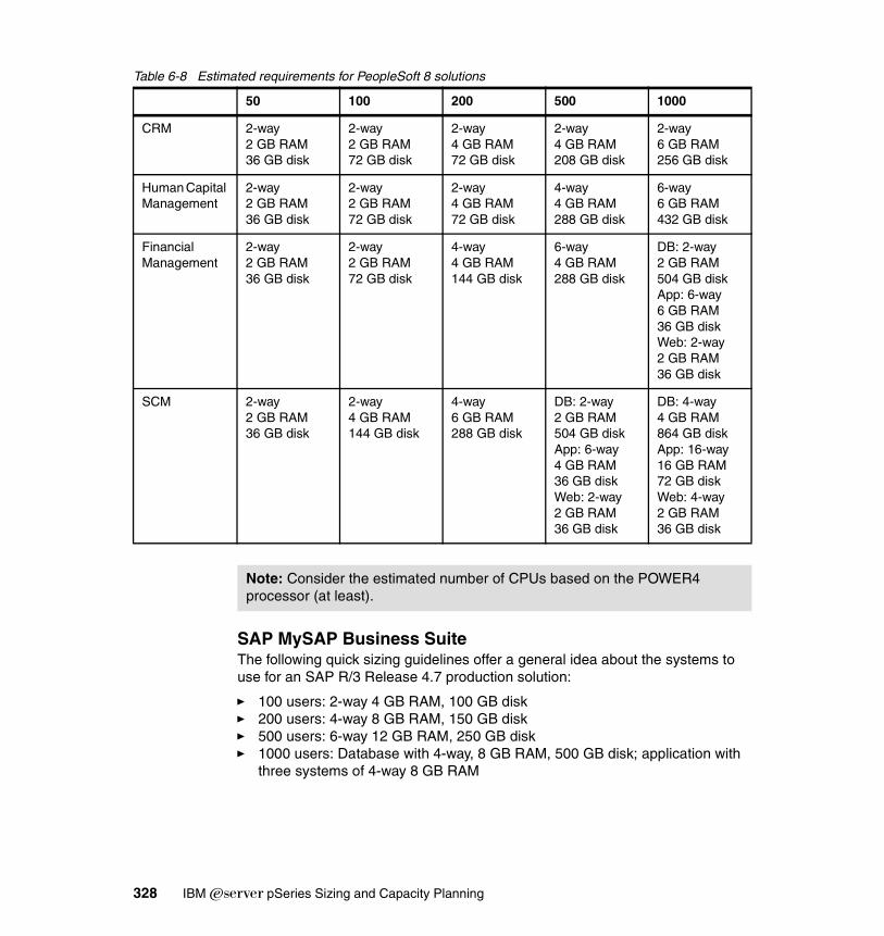
Table 6-8 Estimated requirements for PeopleSoft 8 solutions

SAP MySAP Business SuiteThe following quick sizing guidelines offer a general idea about the systems to use for an SAP R/3 Release 4.7 production solution:

� 100 users: 2-way 4 GB RAM, 100 GB disk� 200 users: 4-way 8 GB RAM, 150 GB disk� 500 users: 6-way 12 GB RAM, 250 GB disk� 1000 users: Database with 4-way, 8 GB RAM, 500 GB disk; application with

three systems of 4-way 8 GB RAM

50 100 200 500 1000

CRM 2-way2 GB RAM 36 GB disk

2-way2 GB RAM72 GB disk



2-way 6 GB RAM256 GB disk

Human Capital Management






Financial Management





DB: 2-way 2 GB RAM504 GB diskApp: 6-way6 GB RAM36 GB diskWeb: 2-way2 GB RAM36 GB disk

SCM 2-way 2 GB RAM36 GB disk



DB: 2-way2 GB RAM504 GB diskApp: 6-way4 GB RAM36 GB diskWeb: 2-way2 GB RAM36 GB disk

DB: 4-way4 GB RAM864 GB diskApp: 16-way16 GB RAM72 GB diskWeb: 4-way2 GB RAM36 GB disk

Note: Consider the estimated number of CPUs based on the POWER4 processor (at least).


These guidelines are based on the following assumptions:

� Sizing scenarios are based on concurrently active users generating two transactions per minute, with the users evenly distributed between financial, controlling, materials management, sales and distribution, and production planning.

� Assumes a ratio of 1 to 4 for database to application workload.

� The database disk estimate does not include RAID 5 or mirroring. On all platforms, we recommend a minimum of 10 disk drives.

6.3 IBM Eserver Sizing GuideThe purpose of the IBM Eserver Sizing Guide is to provide sizing recommendations for IBM Eserver platforms (including pSeries) that run one or more workloads associated with e-business, collaboration, or both. The workloads can represent IBM and ISV applications.

ISVs can find all the necessary information to create Web-based sizing guides using the IBM Eserver Sizing Developer/Estimator. This tool helps to run solutions on IBM Eserver hardware and includes guides as part of the IBM Eserver Sizing Guide. You can find more information on the Web at:

http://www.developer.ibm.com/welcome/eserver/e3/CSFServlet?mvcid=main&packageid=3000

You can use the sizing guide to size a new IBM Eserver system with all new workloads. You can also use it to size the upgrade of an existing system (with the original workload set or any additions) to a new system. The sizing guide recommends the model, processor, interactive feature, memory, and disk necessary for a mixed set of workloads.

To use the Estimator, select one or more workloads and answer a few questions about each workload. Based on your answers, the sizing guide generates a recommendation and shows the predicted CPU utilization of the recommended system. Advanced users can provide more specific information for particular workloads for a more accurate estimate.

When you select your workloads and answer all of the questions for each workload, the sizing guide calculates the results and stores detailed information in the sizing results. These results include a recommended processor model that supports the processing disk and memory requirements of the workload defined.

Note: Consider the estimated number of CPUs based on the POWER4+ processor.



The System Selected page includes the specific processor model, interactive feature, processor utilization, memory, and the required amount of disk.

You can change some of these recommendations for customization. For example, if you want to project for growth, you can adjust the target processor utilization accordingly. After customization, the sizing guide recalculates to determine the best IBM Eserver system options to fit your needs.

Sizing recommendations start with benchmarks and performance measurements based on well-defined, consistent workloads.

As with every performance estimate (whether a rule of thumb or a sophisticated model), you always need to treat it as an estimate. All sizing guide results must still be refined by IBM Technical Sales and IBM Business Partner.

For a search engine of IBM Eserver resources including the IBM Eserver Sizing Guide, see:


You can find the IBM Eserver Sizing Guides on the Web at:


6.4 Network File System sizingNetwork File System (NFS) is a file system implementation that provides remote access to files and file systems. It is probably the most widely used client/server application for sharing data among UNIX systems.

The NFS protocol was developed by Sun Microsystems to allow programs on one system (the NFS client) to access files on another system (the NFS server). The remote directory on the server is mounted to a local directory on the client. The file system on the server looks as though it resides on the local client. Applications can then access files and file systems located on a remote server without copying them locally.

Currently, two widely-implemented and mature versions of NFS exist in the industry. NFS Version 2 (NFS V2) was the only version of NFS available for AIX prior to AIX Version 4.2.1. Limitations to NFS V2, such as the 4 GB file size limitation, the write throughput bottleneck due to synchronous writes, and the need for 64-bit file size support prompted the creation of NFS Version 3 (NFS V3).




NFS V3 supports 64-bit file sizes. Reliable asynchronous writes through WRITE and COMMIT procedures increased throughput considerably when compared to NFS V2.

A fourth version, NFS Version 4 or NFS V4 (defined in RFC 3530), is under development. It is expected that several major vendors will have implementations available sometime in 2004.

Systems running AIX 4.2.1 or later have the option to run either NFS Version 2 or NFS Version 3 over either Transmission Control Protocol (TCP) or User Datagram Protocol (UDP). The functionality and performance differences between NFS V2 and NFS V3, and between TCP and UDP, are some factors to consider when configuring NFS. The combination of the version and protocol to use is controlled primarily via mount options specified by the client.

Less overhead is expected over a UDP mount. However, increased transmit errors or retransmit requests, due to dropped packets or collisions when the network becomes saturated, makes the TCP mount a more robust option in some cases. In the presence of dropped network packets, the more efficient retransmission algorithms of TCP also improve the performance. The default ordering of the protocols was reversed as of AIX 4.3 because of significant performance improvements in TCP over UDP.

6.4.1 FunctionalityFigure 6-3 illustrates the structure of the dialog between NFS clients and a server.

Figure 6-3 NFS client/server interaction


When a thread on a client system attempts to read or write to a file on an NFS-mounted directory, the request is redirected from the normal I/O mechanism to one of the client's NFS block I/O daemons (biod). The biod then sends the request to the appropriate server, where it is assigned to one of the server's NFS daemons (nfsd). On the client, one biod is required to send any read or write request to the server. On the server, an nfsd for each request is dedicated to the biod that sent the request until the request is satisfied and the results of the request are sent back to the client.

For each biod to operate a request, an nfsd must be available to handle that request. Another nfsd may be used by operations (for example, lookups, getattrs) that was not initialized by a biod. The default number of biods per NFS V2 mount is seven, and per NFS V3 is four. The number of biods may be controlled via the biods mount option. As of AIX 4.2.1, the NFS server and client implementations are multithreaded. Therefore, each nfsd and biod is a separate thread, rather than a separate process.

6.4.2 Cache management on an NFS clientTo increase access performance to distributed files, an NFS client keeps the most recently accessed information in its cache. The goal is to avoid other transfers over the network because the information is already on the client.

However, cache coherency must be maintained. Since the server does not keep any record of which clients it services, it cannot alert them when this information is modified. Therefore, it is the job of the client to manage cache coherency.

Read accessEach time a client accesses a file, it must check the coherency between its cache copy and the server's original file. If the copy's last modification time stamp is newer than that of the server file, then it is considered to be good. The data can be served to the application from the NFS client's memory (assuming the data has not been paged out by Virtual Memory Manager (VMM)).

To find this information, NFS uses the open file attributes. That data may also be in the client cache. These attributes have a limited validity. By default, three seconds for a file (acregmin parameter of the mount command) and 30 seconds for a directory (acdirmin parameter of the mount command). If this time information is outdated, the client must ask for it at the server. Then, it compares it to its copy date. If the copy is older than the original, the client must make another call to the server asking for the data.


Write accessIn NFS Version 2, the only way to guarantee server data integrity is to execute the operation synchronously. When an application needs to execute a write operation to a file on an NFS-mounted directory, a biod generates an RPC call on behalf of the application to synchronously execute the write operation on the server. In NFS Version 2, the maximum RPC read and write sizes (rsize and wsize mount parameters) are 8 KB. The call ends only when the server writes the data to non-volatile media.

In NFS Version 3, WRITE and COMMIT procedures allow reliable asynchronous writes and eliminates the synchronous write bottleneck found in NFS Version 2. The NFS client can send multiple WRITE requests and a single COMMIT request when it closes the file. This allows the NFS server to coalesce the client write requests into larger I/Os, which are more efficient than a series of small writes.

The 8 KB data size limitation was also removed in NFS Version 3 to improve performance. The default for per-request size for reads and writes for NFS V3 is 32 KB. You can decrease or configure it up to 60 KB on AIX for mounts over UDP, and up to 64 KB for mounts over TCP.

6.4.3 Performance considerationsOften data is moved to an NFS server because it is relatively easy to do so. However, you must consider the number of users and file accesses across the network. For example, if many users concurrently access a file on the NFS server, there may be lock contention on the file due to exclusive access required on writes. This may result in the users delaying each other from reading or writing from or to the file, and risking a performance degradation.

For optimum performance, use file sharing with NFS primarily in environments where the vast majority of accesses are reads. It is also important to consider the distance between the server and client (in terms of network topology and response times).

AIX Version 4.3 introduced the Cache File System (CacheFS). You can use CacheFS to improve the performance of remote file systems or slow devices such as CD-ROM. When a file system is cached, the data read from the remote file system or CD-ROM is stored in a cache on the local system. This avoids the use of the network and NFS server when the same data is accessed for the

Note: NFS data is cached in the virtual memory manager, as is any data page, but NFS data is never paged to disk space on the client. If a page is selected for pageout and later needed again, it requires another server access to read the data.


second time. An example of where CacheFS is suitable is in a CAD environment, where master copies of drawing components can be held on the server and cached copies on the client workstation when in use.

Selecting the version of NFS (V2 or V3) and the number of nfsds (NFS daemons on the server) and biods (block I/O daemons on the clients), increasing memory, and tuning the disk and logical volume configurations can enhance the NFS system's performance.

You must consider the server capabilities and the typical NFS usage on the client systems when determining how many biods and nfsds to run. Determining an adequate number of nfsds and biods is an iterative process.

Consider these facts:

� By increasing the number of biods and nfsds, you avoid having threads blocked for lack of a biod or nfsd daemon because the biod and nfsd daemons can handle only one request at a time.

� Increasing the number of daemons cannot compensate for a lack of memory, slow processor, or insufficient disk bandwidth.

� All NFS requests go through an nfsd, while only read/write (as well as readdir and readdirplus) operations go through biod.

NFS is based on stateless protocols. A consequence of this is that performance monitoring and management is nontransparent. This means that performance of the clients cannot be measured on the server.

AIX offers various commands to tune and collect NFS statistics, such as netstat, nfsstat, netpmon, and nfso. The UNIX command netstat does not provide information about which are the most resource-hungry clients, but the AIX-specific netpmon command does. Several tunable NFS parameters are available.

6.4.4 Method and sizing factorsThe SPECsfs97_R1 workloads provide a means of contrasting and comparing the NFS-serving capabilities of different systems. Table 6-9 contains the recently published SPECsfs97_R1 results on various pSeries systems.


Table 6-9 pSeries SPECsfs97_R1 results

For example, the table tells us that a 1.7 GHz pSeries 690 16-way has about four times the capacity of a 1.45 GHz pSeries 630-6C4 4-way as an NFS server. However, this statement is specific to the SPECsfs97_R1 workloads. The SPECsfs97_R1.v2 and SPECsfs97_R1.v3 workloads are distinct. Each is characterized by its own mix of NFS operations. For more information, see “The Advancement of NFS Benchmarking: SFS 2.0” by David Robinson, LISA '99 proceedings: 13th Systems.

The results don’t tell you that:

� The pSeries 690 16-way will perform four times better than the pSeries 630-6C4 4-way on any NFS server workload.

� NFS V3 performance is worse than NFS V2 performance on these systems. Nevertheless, a methodology similar to what is used to size the minimum amount of supporting hardware and clients required in a SPECsfs97_R1 benchmark setup may be used for other workloads. See the following sections.

The methodology attempts to remove all memory, I/O, and network subsystem bottlenecks. Therefore, in some cases the amount of equipment used to support this benchmark may seem excessive. The intent is to maximize CPU utilization and remove all I/O wait time.

Obtaining a SPECsfs97_R1 requirementThe easiest requirement to work with is one specified as a SPECsfs97_R1 target. In this case, go to the Standard Performance Evaluation Corporation (SPEC) Web site at:

http://www.spec.org

pSeries models AIX version NFS V2 NFS V3

pSeries 690 16-way (1.7 GHz POWER4+)

AIX 5.2 plus APARs IY36772, IY43591, IY46607, and IY47398

167007 ops/sec (TCP) 136200 ops/sec (TCP)


AIX 5.2 plus APAR IY36772 71075 ops/sec (TCP) 55526 ops/sec (TCP)


AIX 5.2 plus APAR IY36772 58830 ops/sec (UDP) 42706 ops/sec (UDP)


AIX 5.2 plus APAR IY36772 45063 ops/sec (TCP) 33569 ops/sec (TCP)


http://www.spec.org

Looking at the IBM SPECsfs97_R1 results gives you a reasonable indication of a system that is appropriate.

In the absence of this type of requirement, try to gather as much information as possible to improve the accuracy of the sizing. In the case of server replacement and upgrades, analyze the data that is acquired from the current production environment.

Obtaining a system memory requirementIt is difficult to estimate the optimum amount of memory in an NFS serving environment. In general, the more memory there is, the better!

In an established environment, you can use data from iostat (see “Obtaining a storage subsystem throughput or space requirement” on page 336, for disk throughput requirements) to decide if additional memory is helpful. If iostat indicates that a large percentage of I/Os are reads, and the reads are for file system data, then adding memory allows for more caching of this data and reduces the amount of disk I/O.

Obtaining an NFS ops/sec requirementFind an estimate of the number of NFS operations per second that the server must handle by measuring the following items over an interval:

� Measuring client activity (nfsstat -rc)� Measuring server activity (nfsstat -rs)

Pay attention to the mix of operations.

Obtaining a storage subsystem throughput or space requirementUse iostat to gather disk throughput data, including:

� Disk utilization (the tm_act column)� Transactions per second� KB per second� Percentage reads versus writes

For good performance on SPECsfs97_R1, use enough disk adapters and disks to ensure that no disk shows a utilization of more than about 85% busy.

Typically, clients base their storage subsystem needs solely on the amount of space they require. It is important to point out that for optimum performance, consider having sufficient adapters and disk arms (to avoid excessive I/O wait times) and planning for a good file system layout (to spread out I/O load and avoid hot spots). You must understand individual adapter and disk performance characteristics.


Obtaining a network subsystem throughput requirementUse the statistics gathering commands for network adapters (for example, entstat for Ethernet) to access network throughput data, including:

� Packets per second (receive and transmit)� KB per second (receive and transmit)

In terms of KB per second, it is reasonable to expect no more than 60% to 80% of the line capacity per adapter in workloads that consist primarily of large sequential reads/writes (for example, 10000 KB/sec for a 100 Mbps Ethernet adapter running in half-duplex mode). For workloads characterized by accesses that are smaller and more random in nature, you may get no more than 30% to 50% of the line capacity. In these cases, the limiting factor may be the number of packets per second that the adapter can handle. As with disk adapters, it is important to understand the performance characteristics of the network adapters.

Table 6-10 shows estimates of the amount of SPECsfs97_R1.v2 throughput that different network adapters/interfaces can comfortably sustain. These are based on internal benchmark runs.

Table 6-10 Network interface SPECsfs97_R1.v2 capacity

Putting it all togetherHere we look at some of the equipment used for the pSeries 630-6C4 4-way SPECsfs97_R1.v3 TCP workload that is run. The system data used in this analysis was gathered during internal benchmark runs at the peak throughput.

� 24 GB of system memory: The percentage of I/Os that were reads were close to 40%. Based on internal runs with varying amounts of memory, it is possible to achieve similar performance with less memory (as low as 20 GB).

� Two 1 Gbps Ethernet adapters (9000-byte MTU).

� Four 2 Gbps Fibre Channel adapters, Two FAStT700 Storage Server units (each with two controllers), and a total of 140 18.2 GB 15K RPM drives in EXP700 drawers were used in the test configuration. The total system disk throughput at peak NFS ops/sec was approximately 63000 KB/sec and 13000 transactions per second.

The physical disks were divided into RAID 5 arrays (logical disks) of five disks each. A single file system and the related file system log resided on each

Network interface SPECsfs97_R1.v2 ops/sec

100 Mbps Ethernet 3000

1 Gbps Ethernet (1500-byte MTU) 11000

1 Gbps Ethernet (9000-byte MTU) 17000


logical disk, so there were 28 test file systems total in the configuration. The iostat data showed that the logical disks were about 84% busy at peak throughput. Therefore, the storage subsystem layout was adequate.


Part 4 Capacity planning

This part builds on the concepts that are related to capacity planning that were introduced in Chapter 1, “Overview, concepts, and approach” on page 3. It applies these concepts to the capacity planning of pSeries systems.

Part 4



Chapter 7. AIX tools for data gathering

This chapter describes some standard AIX tools, such as vmstat, iostat, sar, svmon, ps, ipcs, and topas. Performance Toolbox, Workload Manager, and Performance Management Services for AIX (PM/AIX) are also covered. These tools provide the ability to collect data that is necessary to properly analyze capacity and sizing requirements for a pSeries system.

7


7.1 AIX standard toolsYou need to identify the components of your workload such as:

� The type of database that your company will use� The kind of software applications that are involved� The number of users that will use the applications� The amount of data that will be handled and from where� The company’s long term plan

You must identify this information to help analyze capacity and sizing. You need to understand the workload of your environment. If you don't, the end result is a waste of your time and money for your company.

Capacity planning and sizing is an art, you must take your time and visualize what you want to accomplish. Time is not something you can save, but in which you can invest. Take your time to plan and visualize what you want to accomplish. The end result of your effort will be rewarding at the end.

Listed here are some of the AIX tools that you need to collect data to analyze your capacity and sizing planning on a pSeries system. Additional various tools are available beyond these, including third-party tools.

The standard AIX tools are:

� vmstat� iostat� sar� svmon� ps� topas

You can save the output of these commands so you can always look back and analyze the data for trends or diagnose a performance issues in a postmortem fashion. The impact and file size are small but the data is valuable after a few weeks for trend spotting.

7.1.1 The vmstat commandThe vmstat command can help you examine CPU, memory, and disk.

For CPUThe vmstat command quickly provides compact information about various system resources and their related performance problems. The vmstat command reports statistics about kernel threads in the run queue and wait queue, memory, paging, disks, interrupts, system calls, context switches, and CPU activity.


The reported CPU activity is a percentage breakdown of user mode, system mode, idle time, and waits for disk input/output (I/O). As a CPU monitor, vmstat command is superior to the iostat command in that its one-line-per-report output is easier to scan as it scrolls. Also, less overhead is involved if there are many disks attached to the system. For example, it can help you identify situations in which a program is spinning or looping or is too CPU-intensive to run in a multiuser environment.

For memoryThe vmstat command summarizes the total active virtual memory (avm) used by all of the processes in the system and the number of real-memory page frames on the free list. Active virtual memory (avm) is the number of virtual-memory working segment pages that were actually touched. This number can be larger than the number of real page frames in the system, because some of the active virtual-memory (avm) pages may have been written to paging space.

When determining if a system may be short on memory or if some memory tuning needs to be done, run the vmstat command over a set interval. Then examine the pi and po columns on the resulting report. These columns indicate the number of paging space page-ins per second and the number of paging space page-outs per second. If the values are constantly non-zero, there may be a memory bottleneck. Occasional non-zero values is not a concern because paging is the main principle of virtual memory.

For diskTo prove that the system disk (not network I/O) is I/O bound, use the iostat command. However, the vmstat command can point to that direction when you look at the wa column.

Command syntaxThe syntax of the vmstat command is:

vmstat [-fsiItv] [Drives] [Interval [Count]]

The following sections explain the flags and parameters of this command.

Important: Active virtual memory is not RAM or available memory. This is a common mistake. avm indicates how much paging space is available.

Chapter 7. AIX tools for data gathering 343

FlagsThe flags of the vmstat command are:

-f Reports the number of forks since system startup.

-s Writes to standard output the contents of the sum structure, which contains an absolute count of paging events since system initialization. The -s option is exclusive of the other vmstat command options.

-i Displays the number of interrupts taken by each device since system startup.

-l Displays an I/O-oriented view with the new columns, p under the heading kthr, and columns fi and fo under the heading page instead of the columns re and cy in the page heading.

-t Prints the time stamp next to each line of output of vmstat. The time stamp is displayed in the HH:MM:SS format, but it is not printed if the -f, -s, or -i flags are specified.

-v Writes to standard output various statistics maintained by the Virtual Memory Manager (VMM). You can only use the -v flag with the -s flag.

You can enter both the -f and -s flags on the command line, but the system only accepts the first flag that is specified and override the second flag.

If the vmstat command is invoked without flags, the report contains a summary of the virtual memory activity since system startup. If the -f flag is specified, the vmstat command reports the number of forks since system startup. The Drives parameter specifies the name of the physical volume.

ParametersThe parameters of the vmstat command are:

� Drives: hdisk0, hdisk1, etc. Disk names can be listed using the lspv command. RAID disks appear as one logical disk drive.

� Interval: Specifies the update period in seconds.

� Count: Specifies the number of iterations.

The Interval parameter specifies the amount of time in seconds between each report. The first report contains statistics for the time since system startup. Subsequent reports contain statistics collected during the interval since the previous report. If the Interval parameter is not specified, the vmstat command generates a single report and then exits.

The Count parameter can only be specified with the Interval parameter. If the Count parameter is specified, its value determines the number of reports generated and the number of seconds apart. If the Interval parameter is specified


without the Count parameter, reports are continuously generated. A Count parameter of 0 is not allowed.

The report generated by the vmstat command contains the following column headings:

� kthr: This indicates the number of kernel thread state changes per second over the sampling interval.

– r: Number of kernel threads placed in run queue.

– b: Number of kernel threads placed in wait queue (awaiting resource, awaiting input/output.

� memory: This offers information about the usage of virtual and real memory. Virtual pages are considered active if they were accessed. A page is 4096 bytes.

– avm: This indicates the number of virtual pages accessed. It does not indicate the available memory.

– fre: This indicates the size of the free list. A large portion of real memory is used as a cache for file system data. It is not unusual for the size of the free list to remain small.

– page: This provides information about page faults and paging activity. It is are averaged over the interval and given in units per second.

– rev: This is the pager input/output list.

– pi: This is the pages paged in from paging space.

– po: This is the pages paged out to paging space.

– fr: This is the pages freed (page replacement).

– sr: This is the pages scanned by page-replacement algorithm.

– cy: This indicates the clock cycles by page-replacement algorithm.

� faults: These are the trap and interrupt rate averages per second over the sampling interval.

– in: Device interrupts– sy: System calls– cs: Kernel thread context switches

� cpu: Breakdown of percentage usage of CPU time.

– us: User time– sy: System time– id: CPU idle time– wa: CPU idle time during which the system had outstanding disk, Network

File Server (NFS) I/O requests.


� Disk: Provides the number of transfers per second to the specified physical volumes that occurred in the sample interval. Use the PhysicalVolume parameter to specify one to four names. Transfer statistics are given for each specified drive in the order specified. This count represents requests to the physical device. It does not imply an amount of data that was read or written. Several logical requests can be combined into one physical request.

If the -I flag is specified, an I/O oriented view is presented with the following column changes:

� kthr: The p column is also displayed in addition to the r and b columns.

– p: Number of threads waiting on actual physical I/O per second.

� page: The new fi and fo columns are displayed instead of the re and cy columns.

– fi: File page-ins per second.– fo: File page-outs per second.

Figure 7-1 shows the output of the following vmstat command:

# vmstat 2 20

Figure 7-1 vmstat output

kthr memory page faults cpu----- ----------- ------------------------ ------------ ----------- r b avm fre re pi po fr sr cy in sy cs us sy id wa 5 2 1314473 464 0 0 0 890 1675 0 897 1443 1471 14 28 48 1119 3 1319978 9158 0 0 0 7924 645410 2011 281356 3408 33 67 0 015 4 1310661 17185 0 0 0 0 0 0 1787 279743 3082 34 66 0 018 2 1310336 14510 0 0 0 0 0 0 3141 278280 4197 32 68 0 012 7 1310335 12588 0 0 0 0 0 0 2116 314908 2400 47 52 0 1 8 8 1307058 12804 0 0 0 0 0 0 2989 233790 2034 42 55 0 411 4 1305770 12709 0 0 0 0 0 0 2063 398786 2649 37 63 0 010 5 1310845 6080 0 0 0 0 0 0 1900 364870 2804 30 70 0 017 3 1300272 14136 0 0 0 0 0 0 2918 291513 3904 34 66 0 014 3 1300708 12387 0 0 0 0 0 0 2054 338995 3674 30 70 0 014 4 1304352 6502 0 0 0 0 0 0 2564 315942 3385 29 71 0 020 3 1312310 409 0 0 0 1783 2813 0 1887 232297 3315 25 75 0 026 2 1310038 2301 0 0 0 900 1455 0 2289 282046 3968 28 72 0 023 3 1303050 7819 0 0 0 0 0 0 1841 198265 3343 31 69 0 0

Note: For a detailed explanation about the vmstat command values, see AIX 5L Performance Tools Handbook, SG24-6039.


7.1.2 The iostat commandThe iostat command is the fastest way to obtain a quick impression about whether the system has a disk I/O-bound performance problem. This command generates reports that you can use to determine an imbalanced system configuration that requires better balance of the I/O load between physical disks and adapters. The tool also reports CPU statistics.

The CPU statistics columns (% user, % sys, % idle, and % iowait) provide a breakdown of CPU usage. This information is also reported in the vmstat command output in the us, sy, id, and wa columns.

Command syntaxThe syntax of the iostat command is:

iostat [-s] [-a] [-d | -t] [-T] [-m] [PhysicalVolume ...] [Interval [Count ]]

The following sections explain the flags and parameters of this command.

FlagsThe flags of the iostat command are:

-a Specifies adapter throughput report.

-s Specifies system throughput report.

-t Specifies TTY/CPU report only.

-T Specifies time stamp.

-d Displays only the disk utilization report.

-m Reports path statistics by device and for all paths. Paths to multipath I/O (MPIO) and the IBM TotalStorage Enterprise Storage Server (ESS) system.

The following conditions exist:

� The -t and -d are mutually exclusive. They cannot both be specified.

� The -s and -a flags can both be specified to display the system and adapter throughput reports.

� If the -a flag is specified with the -t flag, the TTY and CPU report is displayed followed by the adapter throughput report. Disk utilization reports of the disks connected to the adapters are not displayed after the adapter throughput report.

� If the -a flag is specified with the -d flag, the TTY and CPU report is not displayed. If the PhysicalVolume parameter is specified, the disk utilization report of the specified Physical volume is printed under the corresponding adapter to which it belongs.


ParametersThe parameters for the iostat command are:

� Interval: Specifies the update period—the amount of time between each report—in seconds. The first report contains statistics for the time since system startup (boot). Each subsequent report contains statistics collected during the interval since the previous report.

� Count: Specifies the number of iterations. This can be specified in conjunction with the Interval parameter. If Count is specified, the value of Count determines the number of reports generated at interval seconds apart. If Interval is specified without the Count parameter, the command generates reports continuously.

� PhysicalVolume: Specifies disks or paths. This can specify one or more alphabetic or alphanumeric physical volumes. If the PhysicalVolume parameter is specified, the TTY and CPU reports are displayed and the disk report contains statistics for the specified drives. If a specified logical drive name is not found, the report lists the specified name and displays the “Disk is not found” message.

If no logical drive names are specified, the report contains statistics for all configured disks and CD-ROMs. If no drives are configured on the system, no disk report is generated. The first character in the PhysicalVolume parameter cannot be numeric.

TTY and CPU utilization reportThe first report generated by the iostat command is the TTY and CPU Utilization Report. For multiprocessor systems, the CPU values are global averages among all processors. Also, the I/O wait state is defined system-wide and not per processor. The report shows the following information:

� tin: The total number of characters read by the system for all TTYs

� tout: The total number of characters written by the system to all TTYs

� % user: The percentage of CPU utilization that occurred while executing at the user level (application)

� % sys: The percentage of CPU utilization that occurred while executing at the system level (kernel)

� % idle: The percentage of time that the CPU or CPUs were idle and that the system did not have an outstanding disk I/O request

� % iowait: The percentage of time that the CPU or CPUs were idle during which the system had an outstanding disk I/O request


Disk utilization reportThe second report generated by the iostat command is the Disk Utilization Report. This report provides statistics on a per physical disk basis. It shows:

� % tm_act: The percentage of time that the physical disk was active (bandwidth utilization for the drive)

� Kbps: The amount of data transferred (read or written) to the drive in KB per second

� tps: The number of transfers per second that were issued to the physical disk

A transfer is an I/O request to the physical disk. Multiple logical requests can be combined into a single I/O request to the disk. A transfer is of indeterminate size.

� Kb_read: The total number of KB read

� Kb_wrtn: The total number of KB written

System throughput reportThis report is generated if the -s flag is specified. This report provides statistics for the entire system. This report shows:

� Kbps: The amount of data transferred (read or written) in the entire system in KB/sec.

� tps: The number of transfers per second issued to the entire system

� Kb_read: The total number of KB read from the entire system

� Kb_wrtn: The total number of KB written to the entire system

Adapter throughput reportThis report is generated if the -a flag is specified. This report provides statistics on an adapter-by-adapter basis. It contains the following information:

� Kbps: The amount of data transferred (read or written) in the adapter in KB/sec.

� tps: The number of transfers per second issued to the adapter

� Kb_read: The total number of KB read from the adapter

� Kb_wrtn: The total number of KB written to the adapter

Figure 7-2 shows part of the output for the following iostat command:

#iostat -t 2 6

The iostat command is good for performance tuning. However for trend spotting, you need to manipulate the data (add individual disk statistics to obtain a total).


Figure 7-2 iostat command output

7.1.3 The sar commandThe sar command gathers statistical data about the system. You can use this command to gather useful data regarding system performance. However, if the sampling frequency is high, the sar command can increase the system load that can exacerbate a pre-existing performance problem.

Compared to the accounting package, the sar command is less intrusive. The system maintains a series of system activity counters which record various activities and provide the data that the sar command reports. The sar command does not cause these counters to be updated or used. This is done automatically regardless of whether the sar command runs. It merely extracts the data in the counters and saves it, based on the sampling rate and number of samples specified to the sar command.

The sar command provides queuing, paging, TTY, and many other statistics. An important feature of the sar command is that it reports system-wide (global among all processors) CPU statistics (calculated as averages for values expressed as percentages and as sums). It reports statistics for each individual processor. Therefore, this command is particularly useful on symmetric multiprocessor (SMP) systems.

Command syntaxThe syntax of the sar command is:

sar [ { -A | [ -a ] [ -b ] [ -c ] [ -d ][ -k ] [ -m ] [ -q ] [ -r ] [ -u ][ -V ] [ -v ] [ -w ] [ -y ] } ] [ -P ProcessorIdentifier, ... | ALL ][ -ehh [ :mm [ :ss ] ] ] [ -fFile ] [ -iSeconds ] [ -oFile ][ -shh [ :mm [ :ss ] ] ] [ Interval [ Number ] ]

tty: tin tout avg-cpu: % user % sys % idle % iowait 64.6 159.5 13.8 27.5 48.0 10.7 203.5 41797.5 30.5 69.5 0.0 0.0 219.7 31365.8 30.7 69.3 0.0 0.0 244.6 32583.8 38.5 61.5 0.0 0.0 231.5 39152.5 22.0 78.0 0.0 0.0 202.5 34343.3 25.7 74.3 0.0 0.0

Note: For a detailed explanation about iostat command values, see AIX 5L Performance Tools Handbook, SG24-6039.


The following section explains the flags of this command.

FlagsThe flags for the sar command are:

-A Without the -P flag, this flag is equivalent to specifying -abcdkmqruvwy. When used with the -P flag, this flag is equivalent to specifying -acmuw.

-a This flag reports use of file access routines specifying the number of times per second several of the file access routines are called. When used with the -P flag, the information is provided for each specified processor. Otherwise it is provided only system wide.

-b This flag reports buffer activity for transfers, accesses, and cache (kernel block buffer cache) hit ratios per second. Access to most files bypasses kernel block buffering and, therefore, does not generate these statistics. If a program opens a block device or a raw character device for I/O, traditional access mechanisms are used, making the generated statistics meaningful.

-c This flag reports system calls. When used with the -P flag, information for each specified processor is provided. Otherwise, it is provided system wide.

-d This flag reports activity for each block device.

-e hh[:mm[:ss]] This flag sets the ending time of the report. The default ending time is 18:00.

-f This flag indicates file extract records from file (created by -o file flag). The default value of the File parameter is the current daily data file, /var/adm/sa/sadd.

-i Seconds This flag selects data records at intervals as close as possible to the number specified by the Seconds parameter. Otherwise, the sar command reports all seconds found in the data file.

-k Reports kernel process activity.

-m Reports message (sending and receiving) and semaphore (creating, using, or destroying) activities per second. When used with the -P flag, the information is provided for each specified processor. Otherwise, it is provided only system wide.

-o File This flag saves readings in the file in binary form. Each one is in a separate record. Each record has a tag that identifies the reading time.

-P ProcessorIdentifier, ... | ALL This flag reports per-processor statistics for the specified processor or processors. Specifying the ALL keyword reports statistics for each individual processor, and globally for all processors of the flags that specify the statistics to be reported. Only the -a, -c, -m, -u, and -w flags are meaningful with the -P flag.

-q This flag reports queue statistics.


-r This flag reports paging statistics.

-s hh[:mm[:ss]] This flag sets the starting time of the data, causing the sar command to extract records time-tagged at, or following, the time specified. The default starting time is 08:00.

-u This flag reports per-processor or system-wide statistics. When used with the -P flag, information is provided for each specified processor. Otherwise, it is provided system wide. Because this information is expressed in percentages, system-wide information is the average of each processor's statistics. I/O wait state is defined system wide, not per processor.

-V This flag reads the files created by sar on other operating system versions. It can only be used with the -f flag.

-v This flag reports status of the process, kernel-thread, inode, and file tables.

-w This flag reports system switching activity. When used with the -P flag, the information is provided for each specified processor. Otherwise, it is provided system wide.

-y This flag reports TTY device activity per second.

Three scenarios where you can use the sar command are:

� Real-time sampling and display� Display of previously captured data� System activity accounting via cron daemon

Real-time sampling and displayTo collect and display system statistic reports immediately, use the command:

# sar -u 2 5

Figure 7-3 shows the output of this command.

Figure 7-3 Output of the sar command for system statistic reports

AIX ITSO 2 5 000D912F4C00 11/11/03

14:21:23 %usr %sys %wio %idle14:21:27 30 70 0 014:21:29 30 70 0 014:21:32 29 71 0 014:21:35 28 72 0 014:21:38 25 75 0 0

Average 28 72 0 0


To collect and display CPU statistic reports, use this command:

# sar -P ALL 2 10


Figure 7-4 Output of the sar command for CPU statistic reports

Display previously captured dataThe -o and -f options (write and read to or from user-given data files) allow you to visualize the behavior of your system in two independent steps. This

AIX ITSO 2 5 000D912F4C00 05/27/03

13:15:25 cpu %usr %sys %wio %idle13:15:27 0 16 76 5 3 1 34 40 15 11 2 25 54 20 0 3 27 59 0 13 - 25 57 10 713:15:29 0 24 66 7 3 1 25 63 8 4 2 26 63 8 3 3 28 65 4 3 - 26 64 7 313:15:32 0 34 48 6 12 1 26 54 7 14 2 43 44 5 8 3 22 53 10 15 - 31 50 7 1213:15:34 0 26 54 10 10 1 33 47 11 9 2 30 57 7 6 3 25 66 7 2 - 29 56 9 7<...lines of output removed....>13:15:47 0 38 51 6 5 1 34 59 3 4 2 47 46 4 3 3 41 51 2 6 - 40 52 4 5

Average 0 27 59 6 8 1 30 55 6 8 2 34 54 6 6 3 33 54 5 8 - 31 56 6 8


consumes less resources during the problem-reproduction period. You can use a separate system to analyze the data by transferring the file because the collected binary file keeps all data the sar command needs.

The following command runs the sar command in the background, collects system activity data at two-second intervals for five intervals, and stores the (unformatted) sar data in the /tmp/sar.out file. The redirection of standard output is used to avoid a screen output.

# sar -o /tmp/sar.out 2 5 > /dev/null

The following command extracts CPU information from the file and outputs a formatted report to standard output:

# sar -f/tmp/sar.out

The captured binary data file keeps all information that is necessary for the reports. Every possible sar report can be investigated. This allows you to display processor-specific information of an SMP system on a single processor system.

System activity accounting via cron daemonThe sar command calls a process named sadc to access system data. Two shell scripts (/usr/lib/sa/sa1 and /usr/lib/sa/sa2) are structured to be run by the cron daemon and provide daily statistics and reports. Sample stanzas are included (but commented out) in the /var/spool/cron/crontabs/adm crontab file to specify when the cron daemon should run the shell scripts.

The lines in Figure 7-5 show a modified crontab for the adm user. Only the comment characters for the data collections were removed.

Figure 7-5 Modified crontab for the adm user

#===========================================================# SYSTEM ACTIVITY REPORTS# 8am-5pm activity reports every 20 mins during weekdays.# activity reports every an hour on Saturday and Sunday.# 6pm-7am activity reports every an hour during weekdays.# Daily summary prepared at 18:05.#===========================================================0 8-17 * * 1-5 /usr/lib/sa/sa1 1200 3 &0 * * * 0,6 /usr/lib/sa/sa1 &0 18-7 * * 1-5 /usr/lib/sa/sa1 &5 18 * * 1-5 /usr/lib/sa/sa2 -s 8:00 -e 18:01 -i 3600 -ubcwyaqvm &#===========================================================


Collection of data in this manner is useful to characterize system usage over a period of time and to determine peak usage hours.

7.1.4 The svmon commandThe svmon command captures a snapshot of virtual memory. It is useful for determining which processes, user programs, and segments consume the most real, virtual, and paging space memory.

This command is more informative, but also more intrusive, than the vmstat and ps commands. It captures a snapshot of the current state of memory. However, it is not a true snapshot because it runs at the user level with interrupts enabled.

The svmon command can also perform tier and class reports on Workload Manager. It invokes the svmon_back command, which does the actual work, root user and uses trace (only one at a time) for the capacity planning it creates for too much data. If you can’t explain where memory is being used by applications, the svmon command explains everything in great detail.

Here is an example of the svmon command:

# svmon -G


Figure 7-6 Output of the svmon command

Note: For a detailed explanation of sar command values, see AIX 5L Performance Tools Handbook, SG24-6039.

size inuse free pin virtualmemory 4194279 4193776 503 210952 1537865pg space 5529600 36368

work pers clntpin 210950 0 0in use 1808209 2385567 0

Note: For a detailed explanation of svmon command values, see AIX 5L Performance Tools Handbook, SG24-6039.


7.1.5 The ps commandYou can use the ps command to monitor memory usage of individual processes. The ps v Process ID (PID) command provides the most comprehensive report on memory-related statistics for an individual process, such as:

� Page faults� Size of working segment that has been touched� Size of working segment and code segment in memory� Size of text segment� Size of resident set� Percentage of real memory used by this process

Here is an example of the ps command:

# ps v


Figure 7-7 Output of the ps command

The most important columns on the resulting ps report are:

� PGIN: This is the number of page-ins caused by page faults. Since all system calls are classified as page faults, this is basically a measure of I/O volume.

� SIZE: This is the virtual size (in paging space) in 4 KB pages of the data section of the process (displayed as SZ by other flags). This number is equal to the number of working segment pages of the process that were touched multiplied by 4. If some working segment pages are currently paged out, this number is larger than the amount of real memory being used. SIZE includes pages in the private and shared-library data segments of the process.

� RSS: This is the real-memory (resident set) size in 4 KB pages of the process. This number equals the sum of the number of working segment and code segment pages in memory. Remember that code segment pages are shared among all of the currently running instances of the program. If 26 ksh processes are running, only one copy of any given page of the ksh executable program is in memory. But the ps command reports that code segment size as part of the RSS of each instance of the ksh program.

� TSIZ: This is the size of text (shared-program) image and the text section of the executable file. Pages of the text section of the executable program are only brought into memory when they are touched, that is, branched to or

PID TTY STAT TIME PGIN SIZE RSS LIM TSIZ TRS %CPU %MEM COMMAND19612 lft0 A 0:00 18 516 576 xx 41 60 11.5 0.0 vi57682 pts/0 A 0:00 0 336 408 xx 57 72 0.0 0.0 ps v61248 pts/0 A 0:00 0 448 688 xx 201 240 1.2 0.0 -ksh


loaded from. This number represents only an upper bound on the amount of text that can be loaded. The TSIZ value does not reflect actual memory usage. You can also see this value by running the dump -ov command on an executable program, for example:

dump -ov /usr/bin/ls

� TRS: This is the size of the resident set (real memory) of text. It is the number of code segment 4 KB pages. This number exaggerates memory use for programs of which multiple instances are running. The TRS value can be higher than the TSIZ value because other pages may be included in the code segment such as the XCOFF header and the loader section.

� %CPU: This is the percentage of time the process has used the CPU since the process started. The value is computed by dividing the time the process uses the CPU by the elapsed time of the process. In a multiprocessor environment, the value is further divided by the number of available CPUs because several threads in the same process can run on different CPUs at the same time. Because the time base over which this data is computed varies, the sum of all %CPU fields can exceed 100%.

� %MEM: This value is calculated as the sum of the number of working segment and code segment 4KB pages in memory (that is, the RSS value), divided by the size of the real memory of the system in KB, times 100, and rounded to the nearest full percentage point. This value attempts to convey the percentage of real memory being used by the process. Unfortunately, as with RSS, it tends the exaggerate the cost of a process that shares program text with other processes. In addition, rounding to the nearest percentage point causes all processes in the system that have the RSS values under 0.005 times real memory size to have a %MEM of 0.0.

Because many applications use shared memory or memory-mapped segments, the svmon command is a better tool to view memory usage of these segments.

Command syntaxThe syntax for ps command for X/Open Standards is:

ps [ -A ] [ -N ] [ -a ] [ -d ] [ -e ] [ -f ] [ -k ] [ -l ] [ -F format] [ -o Format ] [ -c Clist ] [ -G | -g Grouplist ] [ -m ] [ -n NameList ] [ -p Plist ] [ -t Tlist ] [ -U | -u Userlist ]

Note: The ps command does not indicate memory consumed by shared memory segments or memory-mapped segments. For a detailed explanation about the values, see AIX 5L Performance Tools Handbook, SG24-6039.


The syntax for ps command for Berkeley Standards is:

ps [ a ] [ c ] [ e ] [ ew ] [ eww ] [ g ] [ n ] [ U ] [ w ] [ x ] [ l | s | u | v ] [ t Tty ] [ ProcessNumber ]

The following section explains the flags for this command.

FlagsThe following flags are all preceded by a minus sign (-):

-A This flag writes information about all processes to standard output.

-a This flag writes information about all processes except the session leaders and processes not associated with a terminal to standard output.

-c Clist This flag displays only information about processes assigned to the Workload Manager classes listed in the Clist variable. The Clist variable is either a comma separated list of class names or a list of class names is enclosed in double quotation marks (“ ”) that are separated from one another by a comma, by one or more spaces, or both.

-d This flag writes information to standard output about all processes except the session leaders.

-e This flag writes information to standard output about all processes except the kernel processes.

-F Format This flag is equivalent to the -o Format flag.

-f This flag generates a full listing.

-G Glist This flag writes information to standard output only about processes that are in the process groups listed for the Glist variable. The Glist variable is either a comma-separated list of process group identifiers or a list of process group identifiers enclosed in double quotation marks (“ ”) and separated from one another by a comma or by one or more spaces.

-g Glist This flag is equivalent to the -G Glist flag.

-k This flag lists kernel processes.

-l This flag generates a long listing.

-m This flag lists kernel threads as well as processes. Output lines for processes are followed by an additional output line for each kernel thread. This flag does not display thread-specific fields (bnd, scount, sched, thcount, and tid) unless the appropriate -o Format flag is specified.

-N This flag gathers no thread statistics. With this flag, ps reports statistics that can be obtained by not traversing through the threads chain for the process.

-n NameList This flag specifies an alternative system name-list file in place of the default. This flag is not used by AIX.


-o Format This flag displays information in the format specified by the Format variable. Multiple field specifiers can be specified for the Format variable. The Format variable is either a comma-separated list of field specifiers or a list of field specifiers enclosed within a set of double quotation marks (“ ”) and separated from one another by a comma, one or more spaces, or both. Each field specifier has a default header. The default header can be overridden by appending an equal sign (=) followed by the user-defined text for the header. The fields are written in the order specified on the command line in column format. The field widths are specified by the system to be at least as wide as the default or user-defined header text. If the header text is null (such as though -o user= is specified), the field width is at least as wide as the default header text. If all header fields are null, no header line is written.

-p Plist This flag displays only information about processes with the process numbers specified for the Plist variable. The Plist variable is either a comma-separated list of PID numbers or a list of process ID numbers enclosed in double quotation marks (“ ”) and separated from one another by a comma, one or more spaces, or both.

-t Tlist This flag displays only information about processes associated with the workstations listed in the Tlist variable. The Tlist variable is either a comma separated list of workstation identifiers or a list of workstation identifiers enclosed in double quotation marks (“ ”) and separated from one another by a comma, one or more spaces, or both.

-U Ulist This flag displays only information about processes with the user ID numbers or login names specified in the Ulist variable. The Ulist variable is either a comma-separated list of user IDs or a list of user IDs enclosed in double quotation marks (“ ”) and separated from one another by a comma and one or more spaces. In the listing, the ps command displays the numerical user ID unless the -f flag is used, in which case the command displays the login name. See also the u flag in the following list.

-u Ulist This flag is equivalent to the -U Ulist flag.

The following options are not preceded by a minus sign (-):

a This flag displays information about all processes with terminals (ordinarily only the user’s own processes are displayed).

c This flag displays the command name, as stored internally in the system for purposes of accounting, rather than the command parameters, which are kept in the process address space.

e This flag displays the environment as well as the parameters to the command, up to a limit of 80 characters.

ew This flag wraps the display from the e flag one extra line.


eww This flag wraps the display from the e flag as many times as necessary.

g This flag displays all processes.

l This flag displays a long listing of the F, S, UID, PID, PPID, C, PRI, NI, ADDR, SZ, PSS, WCHAN, TTY, TIME, and CMD fields.

n This flag displays numerical output. In a long listing, the WCHAN field is printed numerically rather than symbolically. In a user listing, the USER field is replaced by a UID field.

s This flag displays the size (SSIZ) of the kernel stack of each process in the basic output format. This value is always zero for a multi-threaded process.

t tty This flag displays processes whose controlling TTY is the value of the TTY variable, which should be specified as printed by the ps command, that is, 0 for terminal /dev/tty0, lft0 for /dev/lft0, and pts/2 for /dev/pts/2.

u This flag displays user-oriented output. This includes the USER, PID, %CPU, %MEM, SZ, RSS, TTY, STAT, STIME, TIME, and COMMAND fields.

v This flag displays the PGIN, SIZE, RSS, LIM, TSIZ, TRS, %CPU, and %MEM fields.

w This flag specifies a wide-column format for output (132 columns rather than 80). If repeated (for example, ww), it uses arbitrarily wide output. This information is used to decide how much of long commands to print.

x This flag displays processes with no terminal.

7.1.6 The ipcs commandThe ipcs command reports status information about active interprocess communication (IPC) facilities. If you do not specify any flags, this command writes information in a short form about currently active message queues, shared memory segments, and semaphores. It is not a performance tool, but can be useful in these scenarios:

� For application developers who use IPC facilities and need to verify the allocation and monitoring of IPC resources

� For system administrators who need to clean up after an application program using IPC mechanisms failed to release previously allocated IPC facilities

Command syntaxThe syntax of the ipcs command is:

ipcs [ -m] [ -q] [ -s] [ -S] [ -P] [ -l] [ -a | -b -c -o -p -t] [ -T] [ -C CoreFile] [ -N Kernel ]


FlagsThe flags for the ipcs command are:

-a This flag uses the -b, -c, -o, -p, and -t flags.

-b This flag reports the maximum number of bytes in messages on queue for message queues, the size of segments for shared memory, and the number of semaphores in each semaphores set.

-c This flag reports the login and group names of the user who made the facility.

-CCoreFile This flag uses the file specified by the CoreFile parameter in place of the /dev/mem file.

-m This flag reports information about active shared memory segments.

-NKernel This flag uses the specified kernel. /usr/lib/boot/unix is the default.

-o This flag reports message queue and shared memory segment information.

-p This flag reports process number information.

-q This flag reports information about active message queues.

-s This flag reports information about active semaphore set.

-t This flag reports time information.

Here is an example of using the ipcs default command:

# ipcs



Figure 7-8 Output of the ipcs command

For an example to determine which processes use shared memory, we can use the -m (memory) and -p (processes) flags together.

# ipcs -mp

The results of this command are shown in Figure 7-9.

IPC status from /dev/mem as of Sun May 25 17:25:03 PST 2003T ID KEY MODE OWNER GROUPMessage Queues:q 0 0x4107001c -Rrw-rw---- root printqShared Memory:m 0 0x580508f9 --rw-rw-rw- root systemm 1 0xe4663d62 --rw-rw-rw- imnadm imnadmm 2 0x9308e451 --rw-rw-rw- imnadm imnadmm 3 0x52e74b4f --rw-rw-rw- imnadm imnadmm 4 0xc76283cc --rw-rw-rw- imnadm imnadmm 5 0x298ee665 --rw-rw-rw- imnadm imnadmm 131078 0xffffffff --rw-rw---- root systemm 7 0x0d05320c --rw-rw-rw- root systemm 393224 0x7804129c --rw-rw-rw- root systemm 262153 0x780412e3 --rw-rw-rw- root systemm 393226 0xffffffff --rw-rw---- root systemm 393227 0xffffffff --rw-rw---- root systemSemaphores:s 262144 0x580508f9 --ra-ra-ra- root systems 1 0x440508f9 --ra-ra-ra- root systems 131074 0xe4663d62 --ra-ra-ra- imnadm imnadms 3 0x62053142 --ra-r--r-- root system...(lines omitted)...s 21 0xffffffff --ra------- root system


Figure 7-9 Output of the ipcs command with the -m and -p flags

7.1.7 The topas commandThe topas command is a performance monitoring tool that is ideal for broad spectrum performance analysis. This command is capable of reporting on local system statistics such as CPU use, CPU events and queues, memory and paging use, disk performance, network performance, and NFS statistics.

The topas command can report on the top hot processes of the system as well as on Workload Manager hot classes. The Workload Manager class information is only displayed when Workload Manager is active. This command defines hot processes as those processes that use a large amount of CPU time. It does not have an option for logging information. All information is real time.

The topas command requires the perfagent.tools fileset to be installed on the system. Figure 7-10 shows the output of this command. It is excellent for performance tuning but not that helpful for capacity planning or trends.

IPC status from /dev/mem as of Sun May 25 11:30:47 PST 2003T ID KEY MODE OWNER GROUP CPID LPIDShared Memory:m 0 0x580508f9 --rw-rw-rw- root system 5428 5428m 1 0xe4663d62 --rw-rw-rw- imnadm imnadm 14452 14452m 2 0x9308e451 --rw-rw-rw- imnadm imnadm 14452 14452m 3 0x52e74b4f --rw-rw-rw- imnadm imnadm 14452 14452m 4 0xc76283cc --rw-rw-rw- imnadm imnadm 14452 14452m 5 0x298ee665 --rw-rw-rw- imnadm imnadm 14452 14452m 6 0xffffffff --rw-rw---- root system 5202 5202m 7 0x7804129c --rw-rw-rw- root system 17070 20696m 8 0x0d05320c --rw-rw-rw- root system 19440 23046

Note: To obtain a meaningful output from the topas command, the screen or graphics window must support a minimum of 80 characters by 24 lines. If the display is smaller than this, then parts of the output become illegible. For detailed explanations of the topas command values, see AIX 5L Performance Tools Handbook, SG24-6039.


Figure 7-10 Output of the topas command

7.2 Performance ToolboxThe Performance Toolbox is a licensed product that allows graphical display of a variety of performance-related metrics. Among the advantages of Performance Toolbox over ASCII reporting programs is that it is much easier to check current performance with a glance at the graphics monitor than by looking at a screen full of numbers. Performance Toolbox also facilitates the combination of information from multiple performance-related commands and allows recording and playback.

Topas Monitor for host: itsosys1 EVENTS/QUEUES FILE/TTYMon Nov 11 10:28:29 2003 Interval: 2 Cswitch 168 Readch 165.0M Syscall 103.5K Writech 41.3MKernel 7.5 |## | Reads 42243 Rawin 0User 73.6 |##################### | Writes 10561 Ttyout 0Wait 1.3 | | Forks 0 Igets 0Idle 17.4 |##### | Execs 0 Namei 0 Runqueue 7.0 Dirblk 0Network KBPS I-Pack O-Pack KB-In KB-Out Waitqueue 1.0en0 0.0 0 0 0.0 0.0lo0 0.0 0 0 0.0 0.0 PAGING MEMORY Faults 5 Real,MB 24575Disk Busy% KBPS TPS KB-Read KB-Writ Steals 0 % Comp 6.5hdisk0 100.0 44432.7 373 0.0 88865.3 PgspIn 0 % Noncomp 19.0hdisk1 97.5 44440.7 373 0.0 88881.4 PgspOut 0 % Client 0.5 PageIn 0WLM-Class (Passive) CPU% Mem% Disk-I/O% PageOut 41 PAGING SPACESystem 77 20 0 Sios 11 Size,MB 12288backups 0 0 0 % Used 0.5 NFS (calls/sec) % Free 99.4Name PID CPU% PgSp Class ServerV2 0ncpu 40532 17.3 0.0 System ClientV2 0 Press:ncpu 41052 10.3 0.0 System ServerV3 0 "h" for helpncpu 44140 10.0 0.0 System ClientV3 0 "q" to quit


Performance Toolbox contains tools for local and remote system-activity monitoring and tuning. The product consists of two main components:

� Performance Toolbox Manager� Performance Toolbox Agent

The agent is also known as Performance AIDE. It must be loaded to the node that needs to be monitored by the manager.

Figure 7-11 shows a simplified local area network (LAN) configuration in which the Performance Toolbox Manager monitors the activity of several systems. Five nodes of a LAN are connected using the star topology. Performance Toolbox Agent is running on each node in the network. One node is the Performance Toolbox Manager and can monitor the other nodes via the resident agent.

The purpose of the Performance Toolbox Manager is to collect and display data from various systems in the configuration. The primary program for this purpose is xmperf. The primary program used by the Agent to collect and transmit data to the Manager is xmservd.

Figure 7-11 LAN configuration with Performance Toolbox

The Performance Toolbox is useful in performing the following functions:

� Capacity planning: Performs long-term monitoring to determine in advance the correct quantity of additional resources required

Agent Agent

Agent Agent

Agent

Manager

xmperf Display


� Load monitoring: Assists in monitoring system resources to detect performance problems

� Analysis and control: When a problem is encountered, determines the correct tool for analyzing the problem and determines the root cause of the problem so that the necessary corrective action can be taken

Other tools that are available in Performance Toolbox are:

� 3dplay: This program plays back 3dmon recordings in a 3dmon-like view.

� chmon: This program is supplied as an executable as well as in source form. It enables monitoring of vital statistics from a character terminal.

� exmon: This program enables monitoring of alarms generated by the filtd daemon running on remote hosts.

� azizo: This legacy recording tool was replaced by jazizo in Performance Toolbox Version 3. It enables you to analyze any recording of performance data and zoom in on sections of the recording. It provides graphical and tabular views of the entire recording or zoomed-in parts of it.

� ptxtab: This program can format statistics from recording files for printing.

� ptxmerge: This program enables merging of up to 10 recording files into one. For example, you can merge xmservd recordings from the client and server sides of an application into one file to better correlate the performance impact of the application on the two sides.

� ptxsplit: In cases where recording files are too large to analyze as one file, this program enables you to split the file into multiple smaller files for better overview and faster analysis.

� ptxrlog: This program create recordings in ASCII or binary format.

� ptxls: This program can list the control information of a recording file, including a list of the statistics defined in the file.

� a2ptx: This program can generate recordings from ASCII files in a format as produced by the ptxtab or ptxrlog programs or the Performance Toolbox for AIX SpmiLogger sample program. The generated recording can then be played back by xmperf and analyzed with jazizo.

� ptxconv: The format of recordings has changed between versions of the Performance Toolbox for AIX. As a convenience to users of multiple versions of the Performance Toolbox for AIX, this program converts recording files between those formats.

� ptx2stat: This tool converts data collected in a recording file to a format that resembles the recording format for the statistic set. It permits postprocessing of data with the programs that enable playback and manipulation of recordings.


� ptxhottab: This program can format and print hot set information collected in recording files.

� wlmperf: This program helps to analyze Workload Management activity from xmtrend recordings. It provides reports on class activity across hours, days, or weeks in a variety of formats. This application is available only in Performance Toolbox Version 3.

7.3 AIX Workload ManagerAIX Workload Manager is an operating system features released with AIX Version 4.3.3 and later enhanced in AIX 5L. It is part of the operating system kernel at no additional charge.

AIX Workload Manager delivers the basic ability to give the systems administrator more control over how scheduler, VMM, and device driver calls allocate CPU, physical memory, and I/O bandwidth to classes based users, groups, application paths, process types, or application tags. It allows a hierarchy of classes to be specified, processes to be automatically assigned to classes by their characteristics, and manual assignment of processes to classes.

Classes can be superclasses or subclasses. AIX Workload Manager self-adjusts when there are no jobs in a class or when a class does not use all the resources that are allocated for it. The resources are automatically distributed to other classes to match the policies of the systems administrator.

Because scheduling is done within a single AIX operating system, system management is far less complex. Unlike logical partitions (LPARs), workload management does not allow multiple operating systems.

AIX Workload Manager is a resource management tool that specifies the relative importance of each workload by classes, tiers, limits, shares and rules. AIX

Note: To learn more about Performance Toolbox, see Performance Toolbox Version 2 and 3 for AIX: Guide and Reference, which is on the Web at:

http://publibn.boulder.ibm.com/doc_link/en_US/a_doc_lib/perftool/prfusrgd/prfusrgd02.htm

Also, see Customizing Performance Toolbox and Performance Toolbox Parallel Extensions for AIX, SG24-2011.

Note: AIX Workload Manager is not a tuning tool. However it can help to speed up a critical applications.


http://publibn.boulder.ibm.com/doc_link/en_US/a_doc_lib/perftool/prfusrgd/prfusrgd02.htm

Workload Manager is ideally suited to balance the demands or requests of competing workloads when one or more resources are constrained. It prevents a relatively uncontrolled way of resource scheduling for different applications on the system. systems administrator are spared from writing complex scripts.

7.3.1 Configuring AIX Workload ManagerTo configure AIX Workload Manager, complete the steps as explained in the following sections.

Step 1: Classify your workloadsFirst, define your classes (superclasses first). You must know your users and their computing needs. Know the applications that are on your system and their resource needs. And, know the requirements of your business (which tasks are critical and which can be given a lower priority).

Step 2: Create the superclasses and assignment rulesTo create the superclasses and assignment rules, use one of the Workload Manager administration interfaces, Web-based System Manager (WebSM), SMIT, or a command line interface (CLI). It takes you through the steps to create your first Workload Manager configuration including defining the superclasses and setting their attributes.

For the first pass, set up only some of the attributes and leave the others at their default value. The same thing applies to the resource shares and limits. You can modify dynamically all of these characteristics of the classes later. The goal is to define a basic set of superclasses and the associated assignment rules.

Then, you can start Workload Manager in passive mode, check your classification, and start looking at the resource utilization patterns of your applications.

Step 3: Use Workload Manager to refine class definitions (passive mode)Check your configuration using the wlmcheck command or the corresponding or WSM menus. Then start Workload Manager in passive mode on the newly-defined configuration. This means that Workload Manager classifies all the existing processes (and all processes created from then on). You can then start monitoring or collection statistics on the CPU, memory, and disk I/O utilization of the various classes, but do not try to regulate this resource usage.

From this point, check that the various processes are classified in the right class as expected by the system administrator (using the -o class option of the ps command). If some of the processes are not classified as you expect, modify


your assignment rules or set the inheritance bit for some of the classes (if you want the new processes to remain in the same class as their parent). Then update Workload Manager. You can repeat this process until you are satisfied with this first level of classification (superclasses).

Running Workload Manager in passive mode and refreshing Workload Manager (always in passive mode) is a low-risk, low-overhead operation. You can do it safely on a production system without disturbing normal system operation.

Step 4: Gather resource utilization dataFor this purpose, run Workload Manager in passive mode using the class definitions resulting from the previous step. Then gather statistics using the wlmstat command. You can start this command to display the per class resource utilization (as a percentage of the total resource available for superclasses) repeatedly and at regular time intervals.

Therefore, you can monitor your system for extended periods to look at the resource utilization of your main applications over time. With this data and your business goals defined in “Step 1: Classify your workloads” on page 368, you can start deciding (or refining) which tier number is given to every superclass and what share and limits of each resource should be given to the various classes.

You can also use the PTX or topas commands to collect Workload Manager data. This is typically all that is required for capacity planning.

Step 5: Turn Workload Manager to active modeYou are now ready to start Workload Manager in active mode. Then you monitor the system again with the wlmstat command. This command checks whether the regulation done by Workload Manager is in line with your goals and whether applications are deprived of resources while others have more than they should. In this case, adjust the tiers shares and limits and refresh Workload Manager.

For specific cases, you may have to use minimum and maximum limits. If possible, try to adjust the shares (and potentially tier numbers) to move closer to your resource allocation goals first. Reserve limits for cases that cannot be solved with shares only. Use minimum limits for applications that typically have low resource usage but need a quick response time when activated by an external event.

A problem faced by interactive jobs in situations where memory becomes tight is that their pages are stolen during the periods of inactivity (waiting for user input, for instance). You can use a memory minimum limit to protect some of the pages of interactive jobs (up to the minimum limit) if the class is in tier 0. Use maximum limits to contain some resource-hungry, low-priority jobs.


Again, unless you want to partition your system resources for other reasons, a hard maximum makes sense mostly for a non-renewable resource, such as memory. This is due to the time it takes to write data out to the paging space if a higher priority class suddenly needs pages that this other class would use. For CPU, use tiers or soft maximum to make sure that, if a higher priority class needs the CPU, it receives it soon.

Monitor and adjust the shares, limits, and tier numbers until you are satisfied with the system's behavior.

Step 6: Fine tune your configurationsYou can decide whether you need to use subclasses and, if you do, whether you want to delegate the subclasses administration for some or all of superclasses. When you create and adjust the parameters of subclasses, you can refresh Workload Manager only for the subclasses of a given superclass without affecting users and applications in the other superclasses.

The administrator of each superclass can repeat the same process described in Step 1: Classify your workloads through Step 5: Turn Workload Manager to active mode for the subclasses of the superclass. The only difference is that it is not possible to run Workload Manager in passive mode at the subclass level only. You may have to perform the subclass configuration and tuning with Workload Manager in active mode. In this case, a way to avoid impacting users and applications in the superclass is to start with the tier number, shares, and limits for the subclasses at their default value—(-) for shares, 0% for min, and 100% for soft and hard max). This way Workload Manager does not regulate the resource allocation between the subclasses.

The Systems Administrator can then monitor and set up the subclasses shares, limits, and tier number as explained in the previous steps.

Step 7: Create other configurations as neededWhen you are done with your initial configuration, you can repeat the process to define other configurations with different parameters for nights and weekends. Or you can repeat the process to define particular peak periods such as the end of quarter or year, according to the needs of the business. When you do this, you may use shortcuts for some steps because you will modify existing configurations.

7.3.2 System capacity and sizing for workload managementWorkload management can be useful in terms of system capacity usage to monitor and collect performance data at the application class level, as input into capacity planning model. Using Workload Manager, you can do this in two ways.


Workload Manager can use the unused portion of system resource that may be wasted in preparation for peak loads if the applications run on separate individual systems. It does this by integrating multiple applications on a single server.

Workload Manager also automates the process of scheduling or rescheduling system resources allocated to lower priority workloads back to high priority (critical) workloads whenever these enter their peak load period. This reallocation process can be so extreme that low priority jobs seem to be stopped. Therefore, the system should be sized sufficiently to handle the combined peak loads of critical workloads. Although some buffering (that is, extra resources) may still be desired to meet increasing resource requirements by critical applications, the amount of consolidated buffer space can be less than the combined buffers of individual systems.

7.3.3 The wlmstat commandTo monitor the statistical resource utilization by each superclass and subclass and to display the status of Workload Manager, use the wlmstat command. This command shows the contents of Workload Manager data structures that are retrieved from the kernel.

Command syntaxThe syntax is:

wlmstat [-l class | -t tier] [-S | -s] [-c | -m | -b] [-B device] [-q][-T] [-a] [-w][-v] [interval] [count]

FlagsThe flags for the wlmstat command are:

-l class This flag indicates the resource utilization for a specific class. If it is not specified, all classes are displayed.

-t tier This flag displays the statistics only for the given tier.

-S This flag displays the statistics for superclasses only.

-s This flag displays statistics for subclasses only. If neither -S nor -s are specified, the statistics for both superclasses and subclasses are displayed. In this case, the statistics for each superclass are listed followed by the statistics for the subclasses belonging to that superclass.

-c This flag shows only CPU statistics.

-m This flag shows only physical memory statistics.

-b This flag shows only disk I/O statistics.


-B device This flag displays statistics for the given disk I/O device. Statistics for all the disks accessed by the class are displayed by passing an empty string (-B “”).

-q This flag represses the output of status files of last action (quiet).

-T This flag (the T for tick) returns the total numbers for resource utilization since each class was created (or Workload Manager started). The units are:

– Number of CPU clock cycles per second used by each class

– Number of memory pages multiplied by the number of seconds used by each class

– Number of 512 byte blocks sent/received by a class for all the disk devices accessed

-a This flag delivers the absolute figures (relative to the total amount of the resource available to the whole system) for subclasses, with a 0.01% resolution. By default, the figures shown for subclasses are a percentage of the amount of the resource used by the superclass, with a 1% resolution. For instance, if a superclass has a CPU target of 7% and the CPU percentage shown by wlmstat without -a for a subclass is 5%, wlmstat with -a shows the CPU percentage for the subclass as 0.35%.

-w This flag displays the memory high water mark. That is the maximum number of pages that a class had in memory since the class was created (or Workload Manager started).

-v This flag shows most of the attributes concerning the class. The output includes internal parameter values intended for AIX support persons. Table 7-1 shows a list of some attributes that may be of interest to users.

interval This flag specifies an interval in seconds (default 1).

count This flag specifies how many times wlmstat prints a report (default 1).

Table 7-1 wlmstat selection of internal parameters

Column header Description

CLASS Class name.

tr Tier number from 0...9.

i Value of the inheritance attribute 0 = no, 1 = yes.

#pr Number of processes in the class. If no process is assigned to a class, the output values, such as CPU, MEM, DKIO, etc., may not be significant.

CPU CPU utilization of the class in percent.

MEM Physical memory utilization of the class in percent.


The results of wlmstat in the normal (non-verbose) case are tabulated with the following fields:

� CLASS: Class name� CPUtotal: CPU time used by the class in percent� MEM: Physical memory used by the class in percent� DKIO: Disk I/O bandwidth used by the class in percent

Consider the following examples. For a report of the current Workload Manager activity, enter this command to see the results in Figure 7-12:

# wlmstat -a

DKIO Physical memory utilization of the class in percent.

DKIO Disk I/O bandwidth utilization for the class in percent.

sha Number of shares. If no (“-”) shares are defined, then sha=-1.

min Resource minimum limit in percent.

smx Resource soft maximum limit in percent.

hmx Resource hard maximum limit in percent.

des Desired percentage target calculated by Workload Manager using the numbers of the shares in percent.

npg Number of memory pages owned by the class.

Note: DKIO is the average of the disk bandwidth on all the disk devices accessed by the class. It is not significant. For example, a class uses 80% of the bandwidth of one disk and 5% of the bandwidth of two other disks. You divide the number of disks that the class is using. Then the value of DKIO for this class is 30%.

For a detailed output of the utilization per disk, use the -B device option.

Column header Description

80percent hdisk1( ) 5percent hdisk2( ) 5percent hdisk3( )+ + 30percent=3 numberofdisk( )

-----------------------------------------------------------------------------------------------------------------------------------------------------------------------------------------------------------


Figure 7-12 Report of current Workload Manager activity

For a report on the superclass backups that are updated every 10 seconds for one minute, enter the following command to see the results in Figure 7-13:

# wlmstat -l backups 10 6

Figure 7-13 Results for superclass backups

For a detailed CPU report of all classes, enter the following command to see the results in Figure 7-14:

# wlmstat -c -v

CLASS CPU MEM DKIO Unclassified 0 15 0 Unmanaged 0 5 0 Default 0 0 0 Shared 0 0 0 System 0 3 0 backups 0 26 0 TOTAL 0 44 0

CLASS CPU MEM DKIO backups 22 3 1 backups 22 3 1 backups 22 4 1 backups 23 5 1 backups 24 6 1 backups 24 7 1


Figure 7-14 Results for CPU report of all classes

For capacity planning, the following options are particularly useful to monitor for a day:

wlmstat 900 96wlmstat -Sv 900 96wlmstat -B “ ” 900 96

7.4 Performance Management Services for AIXThe Performance Management Services for AIX Web-based application is an IBM Global Services Web application and service offering. It reports historical trends of key server resources. It incorporates a series of supplemental programs and techniques that gather local server data, consolidate it into a DB2 database for retention, and enable server utilization reporting directly from the Web. This application also provides reporting on all major IBM server platforms (PM/390 for zSeries, PM/400 for iSeries, PM/AIX for pSeries, and others) while maintaining a consistent look and feel across platforms.

Performance reports provide insight into server utilization trends. They highlight problem areas, enable you to plan for efficient use of existing resources, and identify under-used assets. Reports are divided into two categories: account level and server level. Server-level reports report on a single server, where account-level reports provide data for multiple servers.

CLASS tr i #pr CPU sha min smx hmx des rap urap pri Unclassified 0 0 1 0 -1 0 100 100 100 100 0 10 Unmanaged 0 0 1 0 -1 0 100 100 100 100 0 10 Default 0 0 8 0 -1 0 100 100 100 100 0 0Default.Default 0 0 8 - -1 0 100 100 100 100 0 0 Default.Shared 0 0 0 - -1 0 100 100 100 100 0 0 Shared 0 0 0 0 -1 0 100 100 100 100 0 0 Shared.Default 0 0 0 - -1 0 100 100 100 100 0 0 Shared.Shared 0 0 0 - -1 0 100 100 100 100 0 0 System 0 0 47 0 -1 0 100 100 100 100 0 0 System.Default 0 0 47 - -1 0 100 100 100 100 0 0 System.Shared 0 0 0 - -1 0 100 100 100 100 0 0 backups 0 1 18 20 100 0 100 100 100 100 0 0backups.Default 0 0 18 100 -1 0 100 100 100 100 0 0 backups.Shared 0 0 0 0 -1 0 100 100 100 100 0 0

Note: For a detailed explanation of AIX Workload Manager, see AIX 5L Workload Manager, SG24-5977.


Performance Management Services for AIX uses the dynamic Server Resource Management (SRM) framework and MySRM graphical user interface (GUI) on the Web site to deliver the custom reports. This framework supports enterprise-level views and displays either account-wide report or server-level report views directly from the database.

You can learn more about the Performance Management Services for AIX offering on the Web at:

https://srm.raleigh.ibm.com/pmweb/en/index.jsp

7.4.1 ArchitectureThe Performance Management Services for AIX architecture involves multiple components:

� Data generation� Data collection� Data analysis� Data presentation

Each functional component accommodates processing variables, such as platform data generation options, network access and firewall requirements, database schema requirements, data security, and user reporting presentation options. These components deliver a seamless end-to-end application solution with daily processing to create the reporting deliverables.

7.4.2 UtilizationTo start Performance Management Services for AIX, start your Web browser and go to the following Web address:

http://perf.services.ibm.com

MySRM represents the home page for Performance Management Services for AIX. Its most important components are:

� Performance Reports� Executive with Capacity Reports� Specific Workload Reports� Red Action List

Performance Reports display various daily, weekly, and monthly server resource trends within the chosen enterprise and client scope. Several query options apply to these performance reports:


https://srm.raleigh.ibm.com/pmweb/en/index.jsp

http://perf.services.ibm.com

� Sub client ID1 and sub client ID2: These are used as subgroupings in the enterprise and client hierarchy.

� OS: This is the operating system grouping within the client server grouping.

� Report type: This is the report selection. These include:

– Server Utilization: Processor performance, including memory and paging

– Disk Utilization: Disk summary

– Disk Detail: Detail information (amount used, total size) about all physical volumes in a server

– File System Detail: Detail information (amount used, total size) about all logical volumes or file systems on a server

– Disk I/O Statistics: Disk performance using thresholds

– Processor/Memory Summary: Processor and memory measurements

– Server Trend Report: Processor, memory, and disk utilization measurements

– Resource Utilization: Processor, memory, and disk utilization measurements

– Configuration Summary: Server configuration information

– Server Threshold: Thresholds (or limits) used to determine server exceptions

� Shift: This indicates the time of day performance measurements (prime, off-prime, weekend, all, or N/A).

� Frequency: This indicates the daily, weekly, and monthly reporting period.

� Period ending: This specifies a date range selection for the daily, weekly, and monthly report.

� Red, yellow, and green color symbols: On/off selection is available to filter the server listing, based on color-coded status.

� Report format: You can choose the format for the data display: spreadsheet, graph, or table.

Executive Reports display overall server resource statistics and statistics for processor, memory, and disk utilization. The query panel for selecting these reports may include any of these fields, depending on the characteristics of the client account. Several query options apply to these executive reports:

� Sub client ID1 and sub client ID2: These are used as subgroupings in the Enterprise/Client hierarchy.

� OS: This is the operating system grouping within the client server grouping.


� Report type: This is the report selection. It includes:

– Platform performance– Platform performance detail– Dashboard

� Shift: This is the time of day performance measurements (prime, off-prime, weekend, all or N/A).

� Frequency: This indicates the daily, weekly, and monthly reporting period.

� Period Ending: This specifies a date range selection for the daily, weekly, and monthly report

� Red–Yellow–Green color symbols: On/off selection is available to filter the server listing, based on color-coded status.

� Report Format: You can choose the format for the data display: spreadsheet, graph, or table.

The Specific Workload Reports display performance and capacity statistics for those users who have installed DB2, Lotus, Oracle, or SAP systems.

The Red Action List is a monthly summary of systems that exceeded red thresholds for a resource within the last two months.

With MySRM, data retention is set to seven days of intervals of 15 minutes of data, 35 days of hourly data, 90 days of daily data, 60 weeks of weekly data, and 36 months of monthly data.

With MySRM, thresholds are defined for a variety of characteristics of every server. You can see a report of the thresholds established for any server as Server Threshold Report as a Performance Report at the server level.

The Threshold report shows which metrics contribute to the server’s overall color or status and the thresholds defined for each metric. Where a limit rule is used, the percentage of time that the metric exceeded the limit is displayed. The color settings are also displayed. When a metric has a threshold defined, but no color, the table entry is “No color coding rules apply to this metric.”

7.4.3 Comparison, correlation, forecastMySRM, with the Advanced Report Filter, allows you to make detailed selections regarding your report. You can filter selected columns and rows.

BasicsWithin the Advanced Report Filter, you can make changes to the following selection options:


� Period: The period values change dynamically with the report type selected and the dates of available data. When you click List periods with data, you can see all the dates of available data.

� Show by overall status: Three check boxes are presented. They are called Green, Yellow, and Red. You can select only those that you want to include in your report.

� Report format: You can choose any of several report formats for the output.

ComparisonUse the Comparison Period to see how systems have changed over time. In the report, each numeric value shows the change between the comparison period and the period. The change may be shown as a difference or as a percentage. The change may be presented in a graph and in a table.

You control the Comparison Period from the Advanced Report Filter at the account level only. When viewing a baseline report, consider sorting the various columns to see which ones have changed most.

CorrelationCorrelation is the degree of association between two variables. In simple terms, if two lines on a graph tend to go up and down together, they have a high correlation. If they tend to go up and down opposite of each other, then the correlation is negative. The correlation varies between 0 (no correlation) and ±1.00 (perfect correlation).

The correlation algorithm uses the Pearson Product-Moment correlation. You control the correlation feature from the Advanced Report Filter. Correlation requires at least three data points in the report, although more are recommended.

Correlation can be deceptive. Two variables can have a high correlation by coincidence and not even be related. Conversely, a low correlation does not imply no relation. Moreover, a high correlation between two variables does not imply that one variable causes or predicts the other. Users should be cautious about choosing columns to correlate. Only select pairs of columns that have a linear relationship that is understood.

ForecastThe forecast function uses recorded data to predict data in the future. In a forecasted report, every column is projected into the future. The historical data is shown first, followed by the predicted data.


You control the forecast function from the Advanced Report Filter, at the server level only. Forecasting is only available for server level reports, because only these reports have a time axis. Forecasting is not available in reports for a specific period, such as when the frequency is hourly or every 15 minutes.

There are two types of forecasts:

� Linear regression: This forecast projects as much data into the future as you have in the past. For example, given a week of historical data, linear regression creates one week of predicted data.

� Adaptive regression: This only forecasts as far into the future as is likely to be accurate. It is based on a proprietary algorithm owned by IBM Research.

7.4.4 PM/AIX usagePM/AIX is a service. It is designed to gather data on an AIX system’s performance and capacity, return the data to IBM for analysis, and then deliver reports via the Internet in a presentation that is easy to comprehend. This service uses Server Resource Management to gather data from each monitored system, analyze that data, and present interpreted reports and graphs.

For more information about the PM/AIX service, see:

https://srm.raleigh.ibm.com/pmweb/en/pseries.jsp

7.4.5 Data collectionPerformance and capacity data are collected from each monitored client using Server Resource Management client collection code. Over each 24-hour period, collected data is stored in five unique files:

� dustat: This is the summary of disk usage of physical volumes and space on the file systems. This data is collected once a day.

� iostat: This is the I/O statistics data for all disk drives, including CD-ROM drives. This data is collected every fifteen minutes.

Note: PM/AIX is available on two levels of support:

� IBM Operational Support Services for pSeries performance management (PM/AIX) (a fee service)

� PM/AIX executive summary service: A no-charge easy to implement and use basic performance management process that provides capacity trend information and performance management parameters for pSeries AIX-based servers.


https://srm.raleigh.ibm.com/pmweb/en/pseries.jsp

� netstat: This the network statistics for each defined interface. This data is collected every minute.

� stats: This is the statistics for virtual memory and processor. This data is collected every minute.

� envstat: This is essential system configuration information. Data collected includes basic system identification information, system configuration information, and information about system availability. This data is collected once a day.

Files are stored each day in the /var/adm/perfmgr/daily/[hostname] directory for each client host. They are retained locally on each client for seven days. The task to copy and transmit the collected data files to IBM for analysis is automated.

PM/AIX gathers basic information about the performance and capacity of your AIX systems at the operating system level. No information at the process, user, or application level is collected.

The high-level information that is gathered allows us to provide a high-level analysis of a system’s performance and capacity, while providing the ability to drill down to see greater detail. This data collection is performed with minimal impact to a system’s performance, typically about 1% of the overall system load. The information that is collected is limited to non-proprietary system utilization data coming from the performance monitor data collectors on the system.

7.4.6 ThresholdsTable 7-2 shows the server utilization thresholds used by SRM for AIX servers.

Table 7-2 Server utilization thresholds

Threshold rules Color coding rules

Overall color No threshold rules apply to this metric

The overall color of the server is based on the highest color among the following metrics:� Run queue threshold� Page > Limit/Sec

Processor > Limit

Percentage of time CPU utilization > 90.0%

The metric is red if:� CPU utilization threshold > 50.0 � Run queue threshold > 20.0

The metric is yellow if either of the following are true:� CPU utilization threshold > 50.0 � Run queue threshold > 20.0

Otherwise the metric is green


Table 7-3 shows the disk utilization thresholds used by SRM for AIX servers.

Table 7-3 Disk utilization thresholds

Run Q > Limit Percentage of time run queue > number of processors * 5.0

The metric is red if run queue threshold > 20.0.The metric is yellow if run queue threshold >= 10.0.Otherwise the metric is green.

free/AVM Ratio

Percentage of time free memory < 10% of active virtual memory (AVM)

The metric is red if both:� Free/AVM ratio threshold > 50.0 � Run queue threshold > 20.0

The metric is yellow if either of the following are true:� Free/AVM ratio threshold > 50.0 � Run queue threshold > 20.0

Otherwise the metric is green.

Page > Limit/Sec

Percentage of time page-in rate > 5.0

The metric is red if page-in threshold > 20.0.The metric is yellow if page-in threshold >= 10.0.Otherwise the metric is green.

IO Wait > Limit

Percentage of time I/O wait > 40.0

The metric is red if I/O wait threshold > 50.0.Otherwise the metric is green.



Overall color No threshold rules apply to this metric.

The overall color of the server is based on the highest color among the following metrics:� Hard disk % used� File system % used

Hard disk free No threshold rules apply for this metric.

The metric is red if both:� Physical volume total free < 50.0 � Logical volume total free < 75.0

The metric is yellow if either of the following are true:� Physical volume total free < 50.0 � Logical volume total free < 75.0



7.4.7 SRM reportsThis section presents an overview regarding the SRM reports.

PM/AIX performance reportsTable 7-4 shows the performance reports that you can run on your AIX systems.

Table 7-4 PM/AIX performance reports

Hard disk % used

No threshold rules apply for this metric.

The metric is red if:� Physical volume total percent used > 85.0� Logical volume total percent used > 85.0

The metric is yellow if:� Physical volume total percent used > 85.0 � Logical volume total percent used > 85.0

Otherwise the metric is green

File system free


The metric is red if both:� Logical volume total free < 75.0 � Physical volume total free < 50.0

The metric is yellow if either of the following are true:� Logical volume total free < 75.0 � Physical volume total free < 50.0


File system % used


The metric is red if:� Logical volume total percent used > 85.0 � Physical volume total percent used > 85.0

The metric is yellow if:� Logical volume total percent used > 85.0 � Physical volume total percent used > 85.0



Report name Navigation bar selection

Server level Account level

4-Quadrant Graph Performance S A

Box/LPAR Utilization Performance S A

Box Utilization Performance A


The following sections provide an overview of performance reports that are available with PM/AIX.

4–Quadrant graph reportThis report is beneficial for a quick server status view, especially covering processor and disk utilization. See Figure 7-15 for an example.

Disk Detail Performance S

Disk I/O Statistics Performance S A

Disk I/O Detail Performance S

Disk Utilization Performance S A

File System Detail Performance S

LPAR Disk Utilization Performance S A

LPAR Disk I/O Statistics Performance S A

LPAR Network Traffic Performance S A

LPAR Processor/ Memory Performance S A

LPAR Utilization Performance S A

Network Traffic Performance S A

Network Traffic Detail Performance S

Processor / Memory Performance S A

Resource Utilization Performance S

Server Trend Performance A

Server Utilization Performance S A

Server Utilization by Hour Performance S




Figure 7-15 Sample 4-Quadrant graph report

This set of four graphs provides a status of a server’s health by displaying the reports two-by-two. The four reports are:

� Processor Utilization� File System Utilization� Processor Forecast� 4–Quadrant Graph of processor and file system utilization

The X-axis is for processor utilization. The Y-axis is for file system utilization.

The processor and file system history is determined by the interval selected, such as monthly. The processor forecast graph uses the adaptive regression (or smart forecast) to graph a forecast line into the future, with the future time frame depending on the reporting interval selected, such as monthly or weekly.

The 4-Quadrant Graph plots processor and disk utilization across each of the four quadrants (Q1, Q2, Q3, Q4) in the graph are:

� Q1: Upper Left: Low Processor and High File System utilization� Q2: Upper Right: High Processor and High File System utilization


� Q3: Bottom Left: Low Processor and Low File System utilization� Q4: Bottom Right: High Processor and Low File System utilization

The supported reporting intervals are daily, weekly, and monthly. All, Prime, Off-Prime, or Weekend Shift may be selected.

The key metrics included in this report are Processor Utilization, File System Utilization, Forecasted processor utilization, 4-quadrant graph of processor, and file system utilization.

Box/LPAR utilization reportThis report is beneficial for viewing processor and memory metrics for both the box and its LPARs. This account-level and server-level report shows box and LPAR processor and memory activity for the account, or subaccount, across the reporting interval.

The supported reporting intervals are daily, weekly, and monthly when drilling down to the server level. Fifteen-minute and hourly reports are also available.

The key metrics included in this report are Processor percent used, Memory percent used, and Normalized Processor Value.

Box utilization reportThis report is beneficial for viewing processor and memory metrics for both. This account-level report shows box processor and memory activity for the account, or sub-account, across the reporting interval.

The supported reporting intervals are daily, weekly, and monthly. The key metrics included in this report are Processor percent used, Memory percent used, and Normalized Processor Value.

Disk detail reportThis report is beneficial for allowing the user to examine performance of individual disks on a server. This server-level report shows server hard disk size and usage details. Users can choose the reporting frequency as daily only.

The key metrics included in this report are:

� Physical Volume: The name of the disk that the detail view of the hard disk measurements represent

� Size (of the disk) x Used (amount of MB used)

� Percentage used (portion of the disk)


Disk I/O detail reportThis report is beneficial for allowing the user to troubleshoot intermittent problems on individual disks, by the hour. This server-level report shows the disk I/O utilization details for the server across the reporting interval. Users can only choose the reporting frequency as hourly.


� Percentage Busy� Percentage Time > Limit (percentage busy > 35%)� Kbps� Kbws� TPS

Disk I/O statistics reportThis report (Figure 7-16) is beneficial by allowing the user to examine which disks are exceeding threshold values. This account-level and server-level report shows disk I/O utilization measurements using color-coded key AIX I/O metrics to demonstrate the server’s resource utilization.

Users can choose the reporting frequency as monthly, weekly, or daily. All, Prime, Off-Prime, or Weekend Shift may be selected. If disks exceed 35% busy more than 10% of the time, the server is color-coded yellow.


� Number of Disks on the Server� Average Number of Disks over any Threshold per Exception� Percentage Time Any Disk Over Any Threshold


Figure 7-16 Sample disk I/O statistics report

Disk utilization reportThis report (Figure 7-17) is beneficial for allowing users to examine both the hard disk and file system utilization per server. This account-level and server-level report shows hard disk and file system utilization measurements using color-coded key metrics to demonstrate the server’s resource utilization.

The key metrics for both hard disk and file system included in this report are Size and Percentage used.


Figure 7-17 Sample disk utilization report

File system detail reportThis report is beneficial for a detailed drill-down of specific file system utilization. It may be used in conjunction with the Disk Utilization report that shows the overall File System Utilization. This server-level report shows size and usage details for every file system (or logical volume) on the server, plus the total file system usage. The usage is provided in size used (in megabytes) and by percent utilization.

The Used amount is flagged as green, unless it exceeds the usage threshold (such as 85%), when it is highlighted red. This indicates that further analysis is required to determine whether file system space was sufficient. The supported reporting intervals is daily. The Size Used and % Used fields are color-coded for every logical volume defined on the server. The overall file system utilization is also color coded.

The key metrics included in this report are Total and % Used.


LPAR disk I/O statistics reportThis report is beneficial by allowing user to examine which disks are exceeding threshold values. This account-level and server-level report shows LPAR disk I/O utilization measurements using color-coded key UNIX I/O metrics to demonstrate the server’s resource utilization.

Users can choose the reporting frequency as Monthly, Weekly, Daily, All, Prime, Weekend, or Off-Prime Shift may be selected. If disks exceed 35% busy more than 10% of the time, the server is color-coded yellow.


� Number of Disks on the Server� Average Number of Disks over any Threshold per Exception� Percentage Time Any Disk Over Any Threshold

LPAR disk utilization reportThis report is beneficial for allowing users to examine both the hard disk, and file system utilization per LPAR. This account-level and server-level report shows hard disk and file system utilization measurements using color-coded key metrics to demonstrate the server’s resource utilization.

Users can choose the reporting frequency as Monthly, Weekly, or Daily.

The key metrics for both the hard disk and file system included in this report are Size and Percentage used.

LPAR network traffic reportThis report is beneficial for a quick review of the LPAR network traffic. It covers the server’s Network Card utilization measurements across the account-level and server-level reporting intervals. Overall Status is influenced by the In Packet Errors and Out Packet Errors. The total number of inbound and outbound packets (representing average number of packets transmitted per minute) and associated errors are also measured.

The LPAR Network Traffic Report provides both an account-level and server-level view. At the account level, the LPAR Network Traffic Report measures the utilization across the designated reporting interval. After drilling down to the server level, the Network Traffic Report may be used to display the networking history across the daily, weekly, or monthly reporting intervals.

The key metrics included in this report are In Packet Errors, Out Packet Errors, and Collisions.


LPAR processor/memory reportThis report is beneficial for viewing server detail processor, memory and paging activity. This account-level and server-level report shows LPAR processor, memory and paging activity for the account, or subaccount, across the reporting interval. For each LPAR, there is an individual column for threshold information such as Processor Utilization.

The supported reporting intervals are daily, weekly, and monthly when drilling down to server level. Fifteen-minute and hourly reports are also available. You may need to select the specific operating system to be viewed from the drop-down menu. All, Prime, Weekend, or Off-Prime shift may be selected.

The key metrics included in this report are Processor Util, Run Queue, Page Ins/Sec, Page Outs/Sec, Scan Rate/Sec, and Pages Freed/Sec.

Servers that have configuration data reported display an additional column, Memory Average % Used. This column represents the percentage of real memory in use. Many UNIX variants routinely use most of the real memory and this percentage may be near 100%. This data should only be evaluated in conjunction with the other metrics displayed, such as paging rates, scan rate, and pages freed, for analysis of the server’s memory performance.

LPAR utilization reportThis report is beneficial for a quick review of the LPAR. This account-level and server-level report shows server processor, memory, and threshold measurements for the account (or subaccount) or server across the reporting interval. For each server, there is an individual column for threshold information such as the Observations, Processor Busy, and Processor > Limit, and so on.

The supported reporting intervals are daily, weekly, and monthly. When drilling down to server level, 15-minute and hourly reports are also available. You may need to select the specific operating system to be viewed from the menu. All, Prime, Weekend, or Off-Prime Shift may be selected.

The key metrics included in this report are Processor Utilization, Run Queue, Memory Utilization, Page/Swap Rates, Processor Threshold, Run Queue Threshold, and Paging Threshold. Users can view additional metrics by using the Advanced Report Filter: free/AVM ratio.

Network traffic and network traffic detail reportsThese reports is beneficial for a quick review of the entire account or server and to display the overall view of the account or server’s performance. They cover the server’s network card utilization measurements across both the account-level and server-level reporting interval. The overall status is influenced by the In


Packet Errors and Out Packet Errors. The total number of inbound and outbound packets (representing average number of packets transmitted per minute) and associated errors are also measured.

The network traffic report (Figure 7-18) provides both an account-level and server-level view. At the account level, the network traffic report measures the utilization across the designated reporting interval. After drilling down to the server level, the network traffic report may be used to display the networking history across the daily, weekly, or monthly reporting intervals.

Figure 7-18 Sample network traffic report

If hourly detail is needed to isolate network traffic trends, then the Network Traffic Report is available and displays measurements for each hour in the selected day. This hourly report also provides the Maximum Transmission Unit size, which demonstrates the rate at which packets may be transmitted on the particular network card. The supported reporting intervals are daily, weekly, and monthly (for Network Traffic), plus hourly (for Network Traffic Detail). All, Prime, Off-Prime, or Weekend Shift may be selected.

Network traffic error colors are flagged red if the network error rate exceeds 1% of the volume.


The key metrics included in this report are In Packet Errors, Out Packet Errors, and Collisions.

Processor/Memory reportThis report is beneficial for viewing server detail processor, memory and paging activity. This account-level and server-level report shows server processor, memory and paging activity for the account, or sub-account, across the reporting interval. For each server, there is an individual column for threshold information such as Processor Utilization.

The supported reporting intervals are daily, weekly, and monthly when drilling down to server level. Fifteen-minute and hourly reports are also available. You may need to select the specific operating system to be viewed from the drop-down menu. All, Prime, Off-Prime, or Weekend shift may be selected.


� Processor Util� Run Queue� Page Ins/Sec� Page Outs/Sec� Scan Rates/Sec� Pages Freed/Sec

Servers that have configuration data reported display an additional column, Memory Average % Used. This column represents the percentage of real memory in use. Many UNIX variants routinely use most of the real memory and this percentage may be near 100%. This data should only be evaluated in conjunction with the other metrics displayed, such as paging rates, scan rate, and pages freed, for analysis of the server’s memory performance.

Resource utilization reportThis report (Figure 7-19) is beneficial for viewing server processor, memory, and disk utilization measurements across the reporting interval. This server-level report shows server processor, memory, and disk utilization measurements for the server across the reporting interval.

For each server, there is a column for metric information such as Processor Utilization. Clicking the title of the column provides a drill down to a more detailed explanation of the column. For example, Hard Disk % Utilization indicates, “The average percentage of total disk usage for each system throughout the specified collection period.”

The supported reporting intervals are daily, weekly, and monthly.



� Processor Utilization� Memory Average % Used� Hard Disk % Utilization� File System % Utilization

Figure 7-19 Sample resource utilization report

Server trend reportThis report (Figure 7-20) is beneficial for reviewing up to a six-month trend history for each system of an entire account’s processor utilization, memory, and disk utilization. This account-level report shows server processor, memory, and disk utilization measurements for the account (or sub-account) over a three-month trend history.

Clicking the title of the column provides a drill down to a more detailed explanation of the column. For example Hard Disk (MB)/% Used (five months ago) indicates the average percentage of total disk usage for each system throughout the specified collection period.


Figure 7-20 Sample server trend report

The supported reporting interval is monthly. You may need to select the specific operating system to be viewed from the drop-down menu. All, Prime, Off-Prime, or Weekend Shift may be selected.


� Processor Utilization� Memory Average %� Hard Disk (MB) % Used

Server utilization report and server utilization report by hourThis report is beneficial for a quick review of the entire account or server and to display the overall view of the account or server’s performance. This account-level and server-level report shows server processor, memory, and threshold measurements for the account (or subaccount) or server across the reporting interval. For each server, there is an individual column for threshold information such as the Observations, Processor Busy, and Processor > Limit, and so on.


The supported reporting intervals are daily, weekly, and monthly. When drilling down to server level, 15-minute and hourly reports are also available. You may need to select the specific operating system to be viewed from the menu. All, Prime, Off-Prime, or Weekend Shift may be selected.


� Processor Utilization� Run Queue� Memory Utilization� Page/Swap Rates� Processor Threshold� Run Queue Threshold� Paging Threshold� Active Sessions (Citrix Servers)� Free System Page Table Entries (Citrix Servers)

You can also view the free/AVM ratio metric by using the Advanced Report Filter.

7.4.8 Executive reportsExecutive reports provide a summary of various forms of system usage. They are available for all SRM platforms.

The executive reports contain three columns: Attributes, Performance, and Forecast. In certain cases a fourth column, Availability status, may be present. When the cursor is placed over the color-coded status icon, a window appears, presenting additional summary details. The reports also provide the ability to drill down on client and subaccount ID names to smoothly navigate from high-level status to server-level detail.

The status columns in these reports are defined as follows:

� Performance: This column reflects the overall status of the processor, memory, and disk on the server.

� Forecast: The forecast column projects what the status of the processor value will be in two months for monthly and four weeks for weekly selections. The color coding algorithm for the processor data on the forecast column is: data >= 100.00 is red; data > 80.00; data < 100.00 is yellow; everything else is green. Regardless of the month you choose, the color icons for the forecast do not change because it uses all dates for all servers.

� Availability: The status of this column is derived from the server’s Percent Outage status value.

The Executive reports are available with Executive at Account Level from the MySRM navigation bar.


The following sections five an overview of the Executive reports.

Account status processor utilization reportThis report is beneficial for getting a detail view of the processor utilization trend for all servers in an account. This account-level report shows the processor utilization for all dates for all servers for all accounts selected. This is an account-level report only. Supported reporting intervals are weekly and monthly. This report can be selected only when operating system is set to All. All, Prime, Off-Prime, or Weekend Shift may be selected.

The column fields of this report are Server and the dates of collection.

The key metrics included in this report are Server and Period.

Account status processor utilization by attribute reportThis report is beneficial for getting a detail view of the processor utilization trend for all servers with at least one defined attribute in an account. This account-level report shows the processor utilization for all dates for all servers that have at least one defined attribute, for all accounts selected.

This is an account-level report only. Supported reporting intervals are weekly and monthly. The Operating System selection must be All. All, Prime, Off-Prime, or Weekend Shift may be selected.

The column fields of this report are Server and the dates of collection.

The key metrics included in this report are Attributes, Server, and Period.

Capacity summary all resourceThis report is beneficial for determining an account’s capacity for a given month. This account-level report shows the number of red, yellow, and green servers based on processor, memory, disk, and overall server resource use for the specified account (or sub-account) across the reporting interval. The reporting interval is monthly.

To obtain the capacity summary of servers for given attributes, go to the Advanced Report Filter and select the attributes.


� Red Servers� Percent Red� Yellow Servers� Percent Yellow� Green Servers


� Percent Green� Total Servers

Capacity summary disk reportThis report is beneficial for determining an account’s capacity trend based on the server’s disk use color. This account-level report shows the number of red, yellow, and green servers based on disk resource use for the specified account (or subaccount) across the reporting interval. The reporting interval supported is monthly.


The key metrics included in this report are Red Servers, Percent Red, Yellow Servers, and Percent Yellow.

Capacity summary memory reportThis report is beneficial for determining an account’s capacity trend based on the server’s memory use color. This account-level report shows the number of red, yellow, and green servers based on memory resource use for the specified account (or subaccount) across the reporting interval. The reporting interval supported is monthly.



Capacity summary overall reportThis report (Figure 7-21) is beneficial for determining an account’s capacity trend based on the server’s overall color. This account-level report shows the number of red, yellow, and green servers based on overall server resource use for the specified account (or sub-account) across the reporting interval. The reporting interval is monthly.




Figure 7-21 Sample capacity summary overall report

Capacity summary processor reportThis report is beneficial for determining an account’s capacity trend based on the server’s processor utilization color. This account-level report shows the number of red, yellow, and green servers based on processor resource use for the specified account (or subaccount) across the reporting interval. The reporting interval is monthly.



Dashboard reportThis dashboard style report (Figure 7-22) is beneficial for displaying the overall server status over a 25-month period. It covers the previous 12 months, current month, and forecasted 12-month status.


Figure 7-22 Sample dashboard report

In this report, the color codes use a special capacity planning set of thresholds, which target key individual resource metrics for processor, memory, and disk utilization. The highest threshold exceeded for each resource contributes to the server status and color displayed. By moving the mouse pointer over a color code, you can see the metric values used to calculate the color. At this time, these thresholds are unique and separate from the base Performance Management Services for AIX performance thresholds. They are intended to be more aggressive in detecting capacity exceptions.

Supported reporting interval is monthly. All, Prime, Off-Prime or Weekend Shift may be selected.


� CPU Load� Page/swap Frequency� UNIX Hard Disk� UNIX File System� UNIX Scan Rate

Executive report by accountThis report is beneficial for determining the worst case status of any resource for all servers. It is for all servers and is consolidated by account. The consolidation algorithm is that the highest color (red being the highest and green being the lowest) of all servers having that attribute is set as that column color.

This account-level only report has two frequencies, weekly and monthly. The only operating system value is All. The only shift for this report is Prime.


The key metrics included in this report are Performance and Forecast.

Executive report by attributeThis report is beneficial for determining the worst-case status of any resource for all servers with defined attributes. It displays overall summary status for the server’s performance and forecast metrics for the client’s predefined attribute groupings. Only servers that have attributes are selected for this report. If the selected accounts have no servers with attributes defined, then the report contains no data. Each row is listed by attribute. If an account has only one server with five different attributes, then five rows appear. If an account has 44 servers, with only 10 having defined attributes and only five distinct attributes among them, then only five rows appear in the report.

Each distinct attribute found within an account appears in the report. All following columns in the report are a consolidation of values of the servers in that account found for that attribute. The consolidation algorithm is that the highest color (red being the highest and green being the lowest) of all servers having that attribute is set as that column’s color. The query selects all servers for all dates for that account, with a defined attribute.

This account-level only report has two frequencies, weekly and monthly. The only Operating System value is All. Only Prime Shift may be selected.

The key metrics included in this report are Attributes, Performance, and Forecast.

Executive report by account and attributeThis report is beneficial for determining the worst case status of any resource for all servers with defined attributes. It is similar to Executive Report By Attribute, except that it groups by the account and the attribute, and has the account information listed. If multiple accounts have servers that share common attributes, then those attributes are presented in a row for each account.

This account-level only report has two frequencies: weekly and monthly. The only operating system value is All. Only Prime Shift may be selected.


Executive report by server and attributeThis report is beneficial for determining the worst case status of any resource for all servers with defined attributes. It has the same columns as Executive Report By Attribute. However, the attributes column lists all of the attributes of each


server, as well as account and operating system information. Only servers with attributes are presented in this report.

This account-level only report has two frequencies: weekly and monthly. The only operating system value is All. The only shift for this report is Prime.


Executive report by serverThis report is beneficial for determining the worst case status of any resource for all servers with defined attributes. This report is for all servers. It is grouped by servers and shows the operating system. The consolidation algorithm is that the highest color (red being the highest and green the being lowest) of all servers having that attribute is set as that column’s color.

This account-level only report has two frequencies: weekly and monthly. The only Operating System value is All. The only shift for this report is Prime.

The key metrics included in this report are Performance and Forecast.

Platform performance reportThis report is beneficial for showing the resource status for each server in an account. It displays the overall status and the individual color indicators for the server and in-scope platforms based on processor, memory, and disk values.

This is an account-level only report. Supported reporting intervals are daily, weekly, and monthly. The only operating system value is All. All, Prime, Off-Prime, or Weekend Shift may be selected.

The key metrics included in this report are Status, Processor, Memory, and Disk.

Platform performance detail reportThis report is beneficial for showing the resource status for each server in an account and the values for those resources. It displays the status and the corresponding metric values used to determine the overall status for the in-scope platforms, based on processor, memory, and disk values.

This is an account-level only report. Supported reporting intervals are daily, weekly, and monthly. The only operating system value is All. All, Prime, Off-Prime, or Weekend Shift may be selected.

The key metrics included in this report are Status, Processor, Memory, and Disk.


7.4.9 Capacity reportsCapacity reports are found by choosing Executive Reports in the navigation bar. Like the executive reports, they are available for all platforms, at the server level.

The following sections provide an overview of the Capacity reports.

24-hour profile reportThis report is beneficial for a quick review of the server’s peak utilization times for a given month. It is all hours for Monday through Friday. This server-level report shows the average and maximum processor utilization values for each of the 24 hours in the day across the reporting interval.

The only supported reporting interval is monthly.

Key metrics included in this report: Average Processor Utilization, Maximum Processor Utilization.

Two-year reportThis report is beneficial for a quick review of the server’s peak utilization times for given month. This server-level report shows the average and maximum processor utilization values for every month over a two-year history. Click the title of the column. It provides a drill down to a more detailed explanation of the column (for example, CPU Util (avg.), which is the average CPU utilization during the reporting period).

The only supported reporting interval is monthly.


� Average Processor Utilization (CPU Util (avg.))� Maximum Processor Utilization (CPU Util (max.))

52-week average reportThis report is beneficial for a quick review of the server’s peak utilization weeks over the past year. This server-level report shows the average and maximum processor utilization values for each of the 52 weeks of the past year.

The only supported reporting interval is weekly.


� Average Processor Utilization (CPU Util (avg.) column)� Maximum Processor Utilization (CPU Util (max.) column)


Average free memory reportThis report is beneficial for a quick review of how much free memory a server has and to determine if more needs to be added. This server-level report shows server-level average free memory and installed memory in MB over the reporting interval.

Supported reporting intervals are hourly, daily, weekly, and monthly. All, Prime, Off-Prime, or Weekend Shift may be selected.

The key metrics in this report are Average Free Memory are Installed Memory.

Average paging reportThis report is beneficial for a quick review of how much paging a server is experiencing. This server-level report shows a server’s number of real memory pages per second paged in from the page space and the amount of memory in KB swapped out per second over the reporting interval.

The key metrics included in this report are Average Page In/Sec and Average Page Out/Sec.

Average processor utilization reportThis report is beneficial for a quick review of a server’s processor utilization. This server-level report shows a server’s average system utilization, average user processor utilization, maximum processor utilization during the reporting period.


� Average System Processor� Average User Processor� Peak Processor� Average Processor

Capacity Min/Max reportThis server-level report (Figure 7-23) shows processor utilization with minimum and maximum values based on the report interval used.

Under this report, you can select the following options:

� Frequency: Monthly, Weekly and Daily� Shift: All, Prime, Off-Prime� Measurements: Utilization

Note: The Installed Memory column is populated only if installed memory information is available in the database. If it is not, N/A appears.


Figure 7-23 Sample capacity Min/Max report


� Date: This metric defines the date that data was collected on the server. The formula name for this field is “date”.

� Processor > Limit: This metric defines the percentage of time during collections in which the average processor utilization increased over the “Limit”. The formula name for this field is “processor_2”.

� Minimum processor Utilization: This is the lowest processor utilization value. The formula name for this field is “processor_min”.

� Average processor Utilization: This metric defines the average processor utilization for each system throughout the specified collection period. If the processor utilization averages 100% for the day, it is flagged red as a sign of a possible looping process. In this case, perform further investigations on the system. The formula name for this field is “processor_busy”.

� Maximum Processor Utilization: This is the highest processor utilization value. The formula name for this field is “processor_max”.


File system utilization reportThis server-level Capacity Planning report shows file system usage for each file system averaged over the selected report interval. The reporting interval is daily.


� Disk ID: This is the name of the disk, the detail view of the hard disk measurements represent. The formula name for this field is “disk_id”.

� Average Percentage Allocated: This is the average file system space utilization during the reporting period. The formula name for this field is “avg_pct_alloc”.

� Minimum Percentage Allocated: This is the minimum file system space utilization during the reporting period. The formula name for this field is “min_pct_alloc”.

� Maximum Percentage Allocated: This metric notes the maximum file system space utilization during the reporting period. The formula name for this field is “max_pct_alloc”.

Overall disk utilization reportThis server-level capacity planning report shows average monthly disk usage by file system and by physical disk for the last 12 months. The report interval is daily.


� Date: This is the date that data was collected on the server. The formula name for this field is “date”.

� Hard Disk % Utilization: This is the average percentage of total disk usage for each system throughout the specified collection period. The formula name for this field is “hd_pct_used”.

� File System % Utilization: This is the percentage of file system direct access storage device (DASD) used. The formula name for this field is “fs_pct_used”.

Peak processor regression reportThis report (Figure 7-24) is beneficial for a quick review of the server’s peak utilization times and dates and the values for those times and dates, as well as forecasting the future peak utilization values.

This server-level report shows the peak times of server processor utilization for 30 days up to the current date. It also shows forecast values of peak processor utilization for 30 days into the future. The Time column indicates the time of peak processor utilization for the given Date column. The Processor Util column indicates the Processor utilization value for the system for the specified time. If the Processor utilization averages 100%, it suggests a possible looping process.


In this case, perform further investigation on the system. The formula name for this field is “cpu busy”. The Regression column is a value calculated by linear regression for months with historical data. The formula name for this field is “regression”.

Figure 7-24 Sample peak processor regression report

The only supported reporting interval is hourly.

The key metrics included in this report are Processor Utilization and Regression.

Physical disk utilization reportThis server-level report shows physical disk usage for each hard disk averaged over the selected report interval. The reporting interval is daily.


� Disk ID: This is the name of the disk that the detail view of the Hard Disk measurements represent. The formula name for this field is ”disk_id”.

� Average Percentage Allocated: This is the average Disk System space utilization during the reporting period. The formula name for this field is “avg_pct_alloc”.


� Minimum Percentage Allocated: This is the minimum Disk System space utilization during the reporting period. The formula name for this field is “min_pct_alloc”.

� Maximum Percentage Allocated: This is the maximum Disk System space utilization during the reporting period. The formula name for this field is “max_pct_alloc”.

Processor quartile reportThis server-level report shows processor utilization by quartile and average, as well as maximum run queue utilization. Supported reporting intervals are daily, weekly, and monthly.


� Processor Util: This is the average processor utilization for each system throughout the specified collection period. If the processor utilization averages 100% for the day, it is flagged red as a sign of a possible looping process. In this case, perform further investigations on the system. The formula name for this field is “processor_busy”.

� Processor 25% Quartile: This number represents the first quartile; 25% of the data is equal to or below this value. The formula name for this field is “processor_q25”.

� Processor 50% Quartile: This number represents the second quartile; 50% of the data is equal to or below this value. The formula name for this field is “processor_q50”.

� Processor 75% Quartile: This number represents the third quartile; 75% of the data is equal to or below this value. The formula name for this field is “processor_q75”.

� Maximum processor Utilization: This is the highest processor utilization value. The formula name for this field is “processor_max”.

� Run Q > Limit: This is the percentage of time during statistical collections that the run queue exceeds recommended run queue threshold values. The formula name for this field is “runq_prob”.

Processor regression reportThis server-level report (Figure 7-25) shows actual processor utilization. It also predicts a future regression line for processor utilization, based on the report interval.


� Processor Util: This is the average processor utilization for each system throughout the specified collection period. If processor utilization averages


100% for the day, it is flagged red to indicate a possible looping process. In this case, perform further investigations on the system. The formula name for this field is “processor_busy”.

� Regression: This value is calculated by linear regression for months with historical data. The formula name for this field is “regression”.

Figure 7-25 Sample processor regression report

Week/hour profile reportThis server-level report shows average and maximum processor utilization for each of the 24 hours in a day, averaged over the week interval. The reporting interval is weekly.


� Processor Util (avg.): This is the average processor utilization during the reporting period. The formula name for this field is “processor_util__avg__”.

� Processor Util (max.): This is the maximum processor utilization during the reporting period. The formula name for this field is “processor_util__max_”.


7.4.10 Workload specific reportsThis section provides an overview of the SRM workload specific reports.

DB2 reportsTable 7-5 describes the DB2 reports.

Table 7-5 DB2 reports

Lotus Notes reportsThe Lotus Notes reports display various daily, weekly, and monthly Lotus Notes application trends. Table 7-6 lists the Lotus Notes reports that you can run.

Table 7-6 Lotus Notes reports

The following sections describe the Lotus Notes reports.

Report name

Description

Bufferpool Shows data about each bufferpool defined for the database (bufferpool name, ID and size).

Database Shows information about database activity and includes information about locking activity, memory usage and SQL commands issued. Displays commit/rollback activity, locks and deadlocks, the buffer hit ratio, as well as logical/physical reads and number of SQL statements by type. Key metrics included in this report are Buffer hit ratio, and Deadlocks.

DB space Shows information about the size of the database (total rows and dataspace size used and percent of the database in use). The key metric included in this report is DB Percent Used.

Parameters Shows database parameters in effect (log buffer size, I/O cleaners/servers, sort heap size).

Tablespace Shows tablespace information for each defined tablespace (the tablespace name, the prefetch size, bufferpool ID, tablespace type, and data type).



Database Server Lotus Notes S A

Hourly Concurrent Users Lotus Notes A

Hourly Sessions Lotus Notes A

Mail Hub Server Lotus Notes S A

Mail Server Lotus Notes S

Server Find Server Find A


Database server reportThis report (Figure 7-26) is used to monitor the Lotus Notes mail activity for the Database servers in an account. This account-level and server-level report shows Lotus Notes Database server metrics for the account (or subaccount) or server across the reporting interval.

For each server, there is an individual column for information such as Concurrent Users and Average Sessions per Hour. Clicking the title of the column provides a drill down to a more detailed explanation of the column. For example, Concurrent Users indicates the number of concurrent users who are using Lotus Notes.

The key metrics included in this report are Concurrent Users, Replicated Documents, and Average Sessions per Hour.

Figure 7-26 Sample database server report

Hourly concurrent users reportThis report is used to monitor the Lotus Notes user activity for the Mail or database servers in an account. This account-level report shows the hourly Concurrent Users count for each Lotus Notes Mail or Database server in the specified account (or subaccount) across the reporting interval. It displays the number of Lotus Notes users using the server at each hourly interval. This statistic is generated hourly between 7:00 a.m. and 10:00 p.m.


For each server, there is an individual column for information such as the Concurrent Users, and 7 a.m. Clicking the title of the column provides a drill down to a more detailed explanation of the column.

The supported reporting interval is daily only. The Lotus Notes server type of Mail or Database must be selected.

The key metrics included in this report are Concurrent Users and Average Concurrent Users.

Hourly sessions reportThis report is used to monitor the Lotus Notes session activity for the Database servers in an account. This account level report shows the hourly sessions count for each Lotus Notes Database server in the specified account (or subaccount) across the reporting interval. It displays the number of active Lotus Notes sessions on the server for each hour. This statistic is generated hourly between 7:00 a.m. and 10:00 p.m.

For each server, there is an individual column for information such as the Average Sessions per Hour, and 7 a.m. Clicking the title of the column provides a drill down to a more detailed explanation of the column. For example, Average Sessions per Hour indicates the average sessions per hour.

The supported reporting interval is daily only.

The key metrics in this report are Sessions and Average Sessions per Hour.

Mail Hub server reportThis report is used to monitor the Lotus Notes mail activity for the Mail hub servers in an account. This account-level and server level report shows Lotus Notes Mail hub server metrics for the account (or subaccount) or server across the reporting interval.

For each server, individual column information, such as the Mail Items Routed and Mail Items Sent, is available. Clicking the title of the column provides a more detailed explanation of the column. For example, Mail Items Routed indicates the total number of mail items routed by the hub server.

Supported reporting intervals are daily, weekly, and monthly.


� Mail Items Routed� Mail Items Sent� Incoming Mail� Outgoing Mail


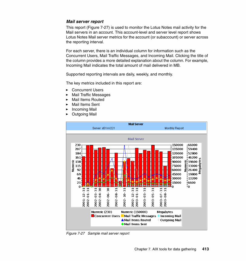
Mail server reportThis report (Figure 7-27) is used to monitor the Lotus Notes mail activity for the Mail servers in an account. This account-level and server level report shows Lotus Notes Mail server metrics for the account (or subaccount) or server across the reporting interval.

For each server, there is an individual column for information such as the Concurrent Users, Mail Traffic Messages, and Incoming Mail. Clicking the title of the column provides a more detailed explanation about the column. For example, Incoming Mail indicates the total amount of mail delivered in MB.

Supported reporting intervals are daily, weekly, and monthly.


� Concurrent Users� Mail Traffic Messages� Mail Items Routed� Mail Items Sent� Incoming Mail� Outgoing Mail

Figure 7-27 Sample mail server report


Oracle reportsThe Oracle reports provide configuration and performance information summarized by hourly, daily, weekly, and monthly intervals. The reports are an overall summary of each database instance for database, workload, tablespace, rollback and parameter data. Table 7-7 includes a list of reports that you can run on your systems running Oracle.

Table 7-7 Oracle reports

The following sections describe the Oracle reports.

Database reportThis report (Figure 7-28) is beneficial for a quick review of the Oracle database performance. It provides buffer pool, sort, tablespace scan, commits, and rollback information for each Oracle instance. The buffer hit ratio is calculated and displayed. Supported reporting intervals are daily, weekly and monthly. When drilling down to detail level by selecting the instance, hourly reports are also available.

All, Prime, Weekend, or Off-Prime shift may be selected.

The key metrics included in this report are Buffer hit ratio, Sort information, and Table scan information.



Database Report Oracle S A

Parameters Report Oracle S

Rollback Report Oracle S

Tablespace Report Oracle S

Workload Report Oracle S A


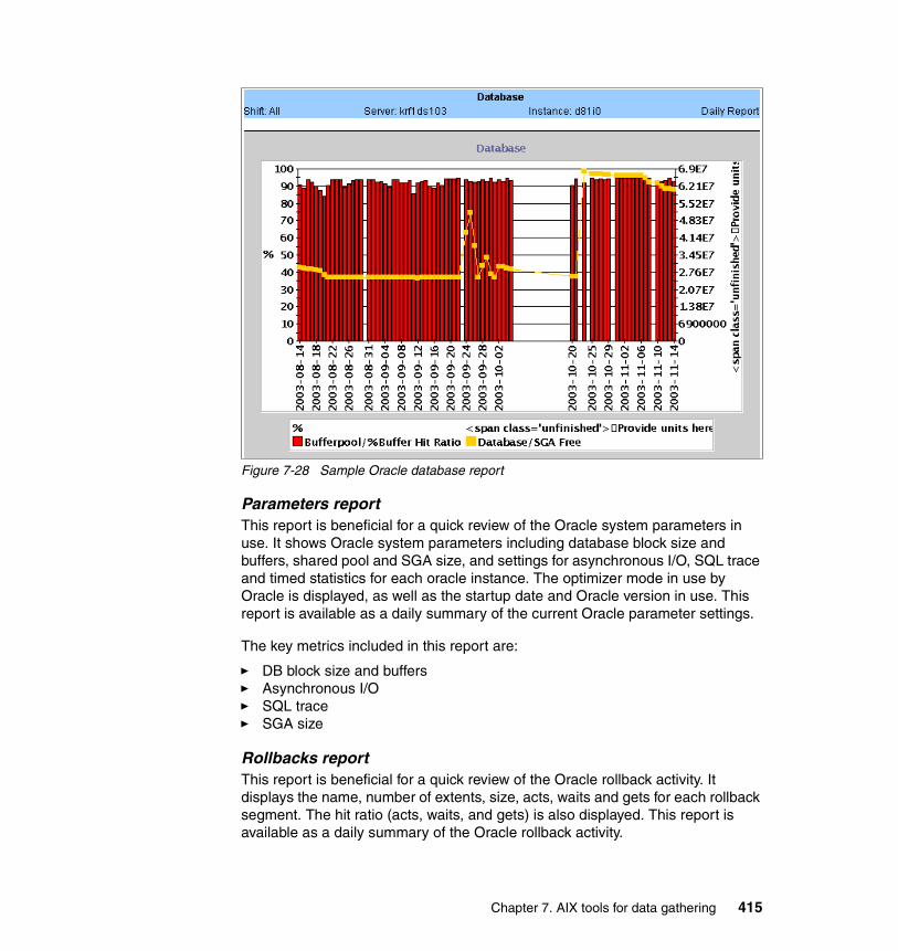
Figure 7-28 Sample Oracle database report

Parameters reportThis report is beneficial for a quick review of the Oracle system parameters in use. It shows Oracle system parameters including database block size and buffers, shared pool and SGA size, and settings for asynchronous I/O, SQL trace and timed statistics for each oracle instance. The optimizer mode in use by Oracle is displayed, as well as the startup date and Oracle version in use. This report is available as a daily summary of the current Oracle parameter settings.


� DB block size and buffers� Asynchronous I/O� SQL trace� SGA size

Rollbacks reportThis report is beneficial for a quick review of the Oracle rollback activity. It displays the name, number of extents, size, acts, waits and gets for each rollback segment. The hit ratio (acts, waits, and gets) is also displayed. This report is available as a daily summary of the Oracle rollback activity.


The key metrics included in this report are Size and % Hit ratio.

Tablespace reportThis report is beneficial for a quick review of the Oracle tablespaces. It displays all defined tablespaces and their size. This report is available as a daily summary.

Workload reportThe Workload report (Figure 7-29) is beneficial for a quick review of Oracle workload and library activity. It provides workload information for users, processes and transactions for each Oracle instance. Library information for gets, hits, pins and reloads are also included. Supported reporting intervals are daily, weekly and monthly. When drilling down to detail level by selecting the instance, hourly reports are also available.

All, Prime, Weekend, or Off-Prime Shift may be selected.

The key metrics included in this report are Gets, Hits, Pins, and Reloads.

Figure 7-29 Sample Oracle workload Report

SAP reportsSAP reports display various daily, weekly, and monthly SAP application trends. All SAP reports are account-level reports. To start any SAP reports, choose SAP in the navigation bar. Table 7-8 shows the available SAP reports with MySRM.

Table 7-8 SAP reports

Report name Description

Internal - Critical Response by Category

Separates the transactions reported into either critical transactions or service transactions; then reports them, summarized by the requested frequency of the report, by category.

Internal - Critical Response by Group

Separates the transactions reported into either critical transactions or service transactions; then reports them summarized by the requested frequency of the report, by group.


Internal - Critical Response Detail

Identifies where slowdowns in response time occur for particular transactions because the report breaks data down to the screen level.

Internal - Dialog Response Time

Daily view of the number of dialog steps executed on an SAP instance, the response time, CPU time and database request for the same instance.

Data availability Shows the number of times that data was collected from each server during a specified time period.

End to End - Critical Response by Category

Separates the transactions reported into either critical transactions or service transactions; then reports them, summarized by the requested frequency of the report, end to end, by category.

End to End - Critical response by Group

Separates the transactions reported into either critical transactions or service transactions; then reports them summarized by the requested frequency of the report, end to end, by group.

End to End - Critical Response Detail

Identifies where slowdowns in response time occur for particular transactions because the report breaks down data to the screen level.

End to End - Overall Dialog Response Time

Determines any trends in performance problems occurring on an SAP instance; identifies workload imbalances among SAP application servers.

Processor Busy Bar Quick review of the poorly performing servers of an SAP instance.

SAP Thresholds Displays values of SAP thresholds used in other SAP reports.

SAP User Quick review of the user workload balance or imbalance on an SAP instance; displays the overall view of the performance of servers comprising an SAP instance.

Top 25 Dialog Transactions by Avg Processor Time

Quick review of the poorly performing transactions on an SAP instance or server.

Top 25 Dialog Transactions by Avg DB Request Time


Top 25 Dialog Transactions by Avg Response Time


Top 25 Dialog Transactions by Total Processor Time


Top 25 Dialog Transactions by Total DB Request Time


Top 25 Dialog Transactions by Total Response Time


Transaction Types Quick review of the transaction workload on an SAP instance; displays the overall view of the SAP instance’s performance.

Report name Description


The following sections review examples with SAP reports.

Dialog response time reportThis report (Figure 7-30) is beneficial for the daily view of the number of dialog steps executed on an SAP instance, the response time, CPU time and Database request for the same instance. This account-level report shows the dialog response times for a selected instance in a continual non-date delimited format. It also shows the daily view of the 110 number of dialog steps executed on an SAP instance, the response time, CPU time and Database request for the same instance. For each client, select Dialog Response Time for the report. Then select the desired SAP instance from the menu. The only frequency choice for this report is Daily, which is the default.


� Dialog Steps� Average Response (ms)� Average Processor (ms)

Figure 7-30 Sample SAP dialog response time report

Internal critical response detail reportThis report (Figure 7-31) is beneficial to identify where slowdowns in response time occur for particular transactions because the report breaks down data to the


screen level. The SAP Critical Response Detail report is similar to the Critical Response by Category report. It shows the same metrics for the individual critical transactions. Because this report has data down to the screen level, it is useful for identifying where slowdowns in response time occur for particular transactions. Such tuning adjustments as improving SQL statements or applying index to a table can be researched and applied to that particular transaction to help improve response times of critical transactions.

Figure 7-31 Sample internal-critical response detail report

Key metrics included in this report (not all of them apply for AIX):

� Dialog Steps� Average Response (ms)

If you are set up for end-to-end reports, response time is reflected as system time. If not, response time reflects end-to-end time. System time is represented by the Average Response field minus the Average Rollwait Time field. It is available with SAP v4.6 and later only.

� Average Processor (ms)� Average Wait (ms)� Average Loadgen (ms)� Average DB Response (ms)� Average Seq Reads (ms)� Percent Under Limit 1 Sec


� Percent Under Limit 2 Sec� Percent Under Limit 3 Sec� Average Rollwait Time (SAP v4.6 and later)� Average Network Time (SAP v4.6 and later)� Average Number Of Trips (SAP v4.6 and later)� Average GUI Response Time (SAP v4.6 and later)

Transaction typesThis report (Figure 7-32) is beneficial for a quick review of the transaction workload on an SAP instance and for displaying the overall view of the SAP instance’s performance. This instance-level report shows the number of dialog steps and the average response time for an SAP instance for transaction types: Batch, Dialog, Spool, and Update.

Figure 7-32 Sample transaction type report

This report helps you understand the volume of workload or distribution of the transaction types on your SAP instance. Excessive numbers of batch type transactions on an SAP instance can affect the response time of online users. This report also helps in identifying problems with the SAP print process (spool). Most important is bottleneck identification. For example, there may not be


enough update processes on an SAP node, resulting in long wait times and slow response time for users.

The key metrics included in this report are Dialog steps, Average Response time.

7.4.11 Application response metric reportsSRM uses application response metrics to provide a detailed look at the response times. This allows the user to look at hourly averages, daily averages, and week and monthly response time averages. SRM also allows the user to correlate the Application Response Time (ARM) metric against a server or a set of servers CPU % metrics. The correlation report is viewable by Application transaction. SRM supports an unlimited number of transactions per application and an unlimited number of applications.

Table 7-9 lists the ARM report types.

Table 7-9 ARM reports

The Application Response Metrics can be provided by any commercial available tool such as IBM EPP or any third-party product that produces application response metrics. SRM admin provides the specific file format needed from these products upon request.

7.4.12 System analysis and forecast with PM/AIXUse the reports in Table 7-10 on system analysis (server or account level).

Table 7-10 PM/AIX reports for system analysis

Report name

Description

Correlation Shows the correlation between the response time and the processor utilization of the servers for a specific application, robot, and transaction. It is obtained only by drilling down on the Transaction value from the account-level Response Time report. Key metrics included in this report are Response Time and Processor Utilization.

Response Time

Shows the hourly breakdown of the transaction response time. Key metrics included in this report are Application, Robot, Transaction, Metric, hours 12 a.m. through 11 p.m.

Report name Report type

Box Utilization (a), LPAR Utilization (sa), Box/LPAR Utilization (sa) PM/AIX Performance

Processor/Memory (sa), LPAR Processor/Memory (sa)Account Status Processor Utilization (a)Capacity Summary Processor (a), Capacity Summary Memory (a)

PM/AIX PerformanceExecutiveExecutive


Use the reports in Table 7-11 for system forecast (server or account level).

Table 7-11 PM/AIX reports for system prediction

The information and conclusions based on the system analysis and forecast with PM/AIX (server and account level) may be materialized in recommendations for:

� System upgrade or replacement� Opportunity for grid computing

The recommendations for grid computing opportunities may be used on the grid computing opportunities evaluation process. For this process, we recommend

Disk Detail (s), Disk I/O Detail (s)Disk I/O Statistics (sa), LPAR Disk I/O Statistics (sa)Disk Utilization (sa), LPAR Disk Utilization (sa)File System Detail (s)Capacity Summary Disk (a)Physical Disk Utilization (s)

PM/AIX PerformancePM/AIX PerformancePM/AIX PerformancePM/AIX PerformanceExecutiveCapacity

Network Traffic (sa), LPAR Network Traffic (sa), Network Traffic Detail (s) PM/AIX Performance

Resource Utilization (s), Server Utilization (sa), Server Utilization by Hour (s)Capacity Summary All Resources (a)Platform Performance (a)

PM/AIX PerformanceExecutiveExecutive

DB2 (Database (s), DB Space (s))Lotus Notes (Database (sa), Mail (s), Mail Hub (sa))Oracle (Database (sa), Workload (sa))SAP (Transaction Type (a), Dialog Response Time (a), Processor busy (a), Top25s (a), Critical Response (a))

Workload Specific



Dashboard (a) Executive

Executive Report by Account, Attribute, Account and Attribute, Server (a) Executive

Red Action List Miscellaneous

Processor Quartile (s), Processor Regression (s), Peak Processor Regression (s), Capacity Min/Max (s)

Capacity

Capacity Summary Overall (a), Capacity Summary Processor (a), Capacity Summary Disk (a)

Executive

4-Quadrant Graph (sa), Server Trend (a) PM/AIX Performance

2-Year (s), 52-week Average (s) Capacity


that you use the IBM Grid Value at Work Tool. Grid Value at Work may help you to identify suitable resources for grid enablement from a larger set, to predict application performance on a grid infrastructure design, to effectuate grid capacity planning analysis.

On the grid computing solution design, you can use the tool to perform what-if analyses of the design: Server type and quantity, Application load and performance, and Grid resource allocation.

As model inputs are made at the IT level, Grid Value at Work includes:

� Application statistics

– Number of job arrivals over a specified time period– Number of parallel tasks in each arriving job– Response time from non-CPU resources needed during parallel tasks– Response time of the sequential (non-grid) portion of each job– As-is (pre-grid) average job response time– Maximum acceptable job response time– CPU service time for each parallel task (on specified server and operating

system)

� Grid server information

– Number of servers, server type/model, and operating system– Relative processing power of each server– Server utilization on non-grid jobs

� Non-grid scenarios

– Number of servers, server type/model, and operating system

As model outputs are made at the IT level, Grid Value at Work uses application performance for:

� Estimated response time� Maximum grid throughput� Grid server utilization� Minimum grid server usage

With Grid Value at Work, multiple applications and grid scenarios alternatives may be modeled at the same time. Grid Value at Work offers support for multiple server allocation algorithms:

� Idle capacity: Sends a job to the server with the most idle capacity (defined by processor power and level of utilization)

� Minimum completion time: Sends a job to the server that can complete it the fastest, accounting for the time spent waiting in the queue


� Utilization threshold: Sends a job to the first server that has utilization below a user-defined threshold

Note: IBM Grid Value at Work is incorporated as part of an IBM Global Services engagement.


Chapter 8. Features and tools for capacity planning

This chapter discusses some AIX features and products that are targeted at capacity planning on pSeries systems. It covers:

� Performance Toolbox � Workload Manager� Dynamic logical partition (DLPAR) and Capacity Upgrade on Demand (CUoD)� IBM Insight tool

8


8.1 Performance ToolboxCapacity planning helps to determine the system resources necessary to achieve the desired performance for a given volume of business transactions. It requires monitoring and analyzing resource usage of the production system. Studying the existing system can also help to determine the system usage trend and the time that a system upgrade is needed.

For effective capacity planning, the tools must be able to:

� Keep enough long-term monitoring data for the user to determine the trend of system utilization and make estimations.

� Analyze the collecting data.

� Select items, time ranges, or both that are interesting.

� Make manipulated data in a generic format for reuse by the other tools such as spreadsheets.

� Make reports containing interesting items selectively.

� Compare the related system resources at one time to help user perception of the correlational effect according to system utilization. The performance of multiple applications working together can be as important as that of an individual application. Therefore, it is important to determine the “big picture” by graphically viewing many correlated parameters concurrently across multiple nodes in a network.

� Automatically have all of these features so a user can perform capacity planning more easily.

Using these tools helps users to increase their productivity. Otherwise, it is time consuming to learn and select the proper commands to monitor target resources usages. Users shouldn’t need to make monitoring scripts. In addition, users don’t need to spend a lot of time manipulating and gathering data for reports to estimate the trends.

Considering these points, Performance Toolbox can be a good solution for capacity planning tools. It provides the following support:

� Monitors and records data using xmtrend, xmservd, xmperf, and 3dmon.

The xmtrend daemon creates long-term and optimized recordings for trend analysis by jazizo and top clients resource by jtopas.

� Analyzes data easily with jazizo, azizo, xmperf, 3dmon, jtopas, and wlmperf.

The jazizo tool is a post-processing application to analyze trend recordings made by the xmtrend daemon. It is ideal for monitoring long-term performance. The xmperf tool is, at the same time, a graphical monitor, a tool


for analyzing system load, and an umbrella for other tools, regardless of whether they are performance related.

� Selects interesting items and time ranges from complex and enormous recording data with jazizo, azizo, and wlmperf.

� Converts to tabulated format, ASCII format, or both so users can use the converted data with other tools with ptxrlog and ptxtab.

The ptxtab tool allows users to convert the recording into a comma- or tab-delimited spreadsheet format that can be imported into third-party spreadsheet applications.

� Makes reports with ptxrlog and ptxtab.

� Compares the related system’s resource at one time with 3dmon, jtopas, and ptxmerge.

The 3dmon tool allows the monitoring of a large number of statistics in a single window. The jtopas tool is a client to view top resource usage on local and remote systems. This application can show real time and recorded data.

� Has several predefined monitoring entries, and records the analyzing method. Users need only to select the monitoring entries and rules. Performance Toolbox can do various things automatically.

As discussed in 7.2, “Performance Toolbox” on page 364, Performance Toolbox consists of a set of agents and utilities to collect, filter, record, and report performance metrics. Its primary agent, xmservd, can record metrics specified in a configuration file. The configuration file specifies the metric name, start time, stop time, days to record, recording frequency, and other items. Performance Toolbox analyze tools and recording data converting tools can perform post processing of recordings.

Several benefits derived from using Performance Toolbox as explained in the following sections.

Monitoring featuresThe client/server environment allows any program, whether part of Performance Toolbox for AIX or custom developed applications, to monitor the local host and multiple remote hosts.

This ability is fully explored in the Manager component program xmperf. The “monitors” of xmperf are graphical windows, referred to as consoles. You can customize consoles on the fly or keep them as pre-configured consoles that you can invoke with a few mouse clicks. Consoles can be generic so the actual resource to monitor, whether a remote host, a disk drive, or a local area network (LAN) interface, is chosen when the console is opened. Consoles can make a

Chapter 8. Features and tools for capacity planning 427

recording, of the data they monitor, to disk files. Such recordings can be played back with xmperf and analyzed with the jazizo program.

One of the things that makes xmperf unique is that it is not hard coded to monitor a fixed set of resources. It is dynamic in the sense that a system administrator can customize it to focus on exactly the resources that are critical for each host that must be monitored.

An implementation of the Application Response Management (ARM) specification allows applications to be instrumented so that the activity and response times of applications can be monitored. In addition, the raw response time from any host running the Performance Toolbox agent to any Internet Protocol (IP)-capable host in the network can be monitored.

Another feature is the Agent filter called filtd. It allows you to easily combine existing “raw” statistics into new statistics that make more sense in your environment. You do this by entering simple expressions in a configuration file and requires no programming.

Analysis and control of system performance The manager program xmperf provides an umbrella for tools that can be used to analyze performance data and control system resources. In doing so, it assists the system administrator tracking the available tools and applying them in appropriate ways. They do this through a user-configurable menu interface.

Tools can be added to menus. This is done with fixed sets of command line arguments to match specific situations. Or it can be done so that the system administrator has an easy way to remember and enter command line arguments in a window. The xmperf menus are preconfigured to include most of the performance tools shipped as part of the tools option of the Agent component.

Properly customized, xmperf becomes an indispensable repository for tools to analyze and control an operating system. In addition, the ability to record load scenarios and play them back in graphical windows at any desired speed provides new and improved ways to analyze a performance problem.

Recordings can be produced from the monitoring programs xmperf and 3dmon during monitoring. Or they can be created by the xmservd daemon. This makes constant recording possible so that you can analyze performance problems after they occur. The 3dplay program is provided to play back recordings created by 3dmon in the same style in which the data was originally displayed. Outstanding features for analyzing a recording of performance data are provided by the jazizo program and its support programs.


Finally, using the Agent component filter filtd, you can define conditions that, when met, can trigger any action that you deem appropriate. This includes alerting yourself or initiating corrective action without human intervention. This facility is entirely configurable so that you can customize alarms and actions to your installation.

Capacity planningIf your system is capable of simulating a future load scenario, you can use xmperf to visualize the resulting performance of your system. By simulating the load scenario on systems with more resources, such as more memory or disks, the result of increasing the resources can be demonstrated. Long-term capacity requirements must be analyzed so sufficient resources can be acquired well before they are required.

8.1.1 Tool utilization strategyAs you begin to form your monitoring strategy, determine how broad a view of your system resource utilization’s data is necessary. Also, consider how long you need recording data to estimate trends. Plus, know the kind of resources that you you need to gather.

If you recorded information, what kind of tools and functions you do want to use? Some tools are included with the manager code (xmperf, 3dmon). Others are packaged with the agent code (ptxtab, ptxsplit, etc.). Still other useful tools for data analysis, such as database, spreadsheets, perl or statistical analysis programs such as SAS, are not provided with Performance Toolbox. But you can make and the record the system utilization data for those tool (ptxrlog, ptxtab).

Performance Toolbox has two kinds of tools for analyzing. One is suitable for the short term such as xmperf and 3dmon. The other is suitable for the long term and capacity planning such as azizo, jazizo, and wlmperf.

This chapter concentrates on long-term related functions for capacity planning among several Performance Toolbox functions. Such functions are ideal to monitor system for the long term.

For more information about the basics of Performance Toolbox and other functions, see Performance Toolbox Version 2 and 3 Guide and Reference, SC23-2625, or AIX 5L Performance Tools Handbook, SG24-6039.

8.1.2 azizoThe azizo is a program for analyzing recordings made by the agent or manager program. It analyzes one recording file at a time. If multiple recordings must be


analyzed together, the support program ptxmerge can merge multiple recording files into one for simultaneous analysis of statistics from multiple sources.

When recording files contain console definitions, the definitions are not usable in the analysis performed by azizo. They are ignored, except when a filtered recording is produced. All other record types in recording files are used to build the data tables used in the analysis.

Whenever azizo reads a recording file, it first finds all the statistics defined in the file. For each statistic, it builds a table with a number of elements corresponding to the width of the graph area.

Recording files are binary files whose first record is a configuration record. This record identifies the file as a recording file, names the source of the recording, and states the version of the file. Recording files are created by one of the agent or manager programs.

8.1.3 xmtrendThe xmtrend daemon can record system performance data. It permits any system with the Agent component installed to record the activity on the system at all or selected times and for any set of performance statistics. This allows a system administrator to use the activity recording for an after-the-fact analysis of the performance problems.

The xmtrend agent was created to focus on providing manageable 24 x 7 long-term recordings of large metric sets. These recordings are used by jazizo, jtopas, and other analysis tools supporting the trend recording format. The user specifies in a configuration file which statistics are to be recorded. The daemon then automatically computes and records the maximum, minimum, mean, and standard deviation for each listed metric, across a frequency specified by the user. The xmtrend agent uses the Spmi interface to request data at an internal cycle rate of at least once per second. For xmtrend, this cycle rate is independent of the recording frequency specified by the user, which by default is once every 10 minutes.

All recording files created by xmtrend are placed in the /etc/perf directory unless otherwise specified. Recording file names are of the format xmtrend.yymmdd for xmtrend. The part after the period is built from the day the first record was written

Note: The azizo recording application has been replaced with the Java-based jazizo application in Performance Toolbox for AIX Version 3. This new tool provides more functionality than azizo and is easier to use. The jazizo application processes long-term, large metric set recordings from the xmtrend daemon.


to the file. The recording activity for any one day always goes to the same file, even when xmtrend is stopped and started over the same day. If a recording file for the day exists when xmtrend starts, it appends additional activity to that file; otherwise it creates the file.

Recordings produced by xmtrend have one or more sets of statistics. One is created for each recording interval defined in the recording configuration file. Each set of statistics is assigned a number that is equal to the recording interval divided by the minimum sampling interval of the daemon.

Recording configuration fileThe system administrator who configures a host must supply the recording configuration file. No recording configuration file is supplied as part of the Performance Toolbox for AIX. The file is in ASCII format.

When xmtrend starts, the xmtrend agent looks for the /etc/perf/xmtrend.cf configuration file. If it is not found, the program exits. A sample configuration file is provided in /usr/lpp/perfagent/xmtrend.cf. The xmtrend agent has some command line arguments to allow the user to specify where xmtrend should look for the configuration file.

The recording configuration file must contain the following lines:

� One retain line� One frequency line� One or more metric lines� One or more start and stop lines

The recording configuration file may also contain:

� One or more command lines� One or more hot lines

For more information about configuration file lines, see Performance Toolbox Version 2 and 3 Guide and Reference, SC23-2625.

8.1.4 jazizoThe jazizo command is a post-processing application for analyzing trend recordings made by the xmtrend daemon. It is a new tool to analyze the long-term performance characteristics of a system on Performance Toolbox V3.0. It is suitable for analyzing system statistics over a long period of time.

The jazizo command uses the xmtrend daemon to collect data and provides user configurable displays of the recorded data. Jazizo can be configured to show only the data of interest, in clear and concise graphical or tabular formats.


Users can create, edit, and save custom configurations. In addition, reports can be generated covering specific time periods. Data reduction options are provided to assist analysis.

The jazizo program resides in /usr/bin. It is part of the perfmgr.analysis.jazizo fileset, which is installed from the Performance Toolbox Version 3 for AIX media. The perfmgr.common and perfagent.server filesets are prerequisites for perfmgr.analysis.jazizo.

The Performance Toolbox agents can collect hundreds of performance metrics that are available from the pool of resources available on a system. Jazizo was created to provide a simple user interface for analyzing recorded performance data over extended periods of time, primarily focused on aiding trend analysis. Specifically, jazizo can be used to graphically view resource usages over hours, days, weeks, or months to help determine if resources are, or will be, constrained. It can also identify recurring peak usage periods and allows you to review them.

The syntax is:

jazizo [ -r RecordingFile [ -c ConfigurationFile ]]

Here -r RecordingFile is a file created by xmtrend or a directory that contains xmtrend recording files. -c ConfigurationFile is a file that describes both metric and graph options.

Examples of using jazizoThis section introduces examples of using jazizo, focusing only on the interesting steps in terms of capacity analyzing. To learn more details about jazizo, see the AIX 5L Performance Tools Handbook, SG24-6039.

If the command is issued without any flags, the jazizo program searches for a configuration file to determine which metrics are to be displayed. At this point, it is important to remember that the xmtrend daemon gathers the data, while the jazizo program displays the results.

If you open the recording file using jazizo, the Metric Selection window shows a list of metrics that can be displayed as shown in Figure 8-1. To display the metrics, you add them to the right-hand pane. Click Add to move the selected metrics. In the same way, you can remove an incorrectly selected metric from the right-hand pane. Select the metric and click Remove.

The file that contains the data on the metrics can have data that spans several months, up to a year, so date and time selections are available to crop the view to display only a required period. You can click the Edit Start/Stop button to select the Start Hour and Stop Hour for the period to be displayed.


Figure 8-1 Metric selection window

On the Time Selection window (Figure 8-2), select the time and date. Click OK to close the window. Back on the Metric selection window (Figure 8-1), click Apply.

Figure 8-2 The time selection window


The jazizo program now displays the selected metrics over the selected monitoring period, as shown in Figure 8-3. In this example, we select three CPU related metrics: glidle, glkern and gluser. The vertical axis of the graph is shown in graduations of 10. It is in percent because this graphic is displaying CPU percentage statistics. The horizontal axis has a time graduation over the selected monitor period.

Each of the selected metrics in this example is represented by a colored line graph. At the bottom of the window, the metrics are listed with the appropriate colored selection blocks. These selection blocks are the same color as the line of the graph. The selection block is used to select the specific metric on the graph. The name of the particular metric is followed by its range minimum and maximum in parentheses.

Figure 8-3 The jazizo window


As shown in Figure 8-4, select Edit-> Metric Selection to open the Metric Selection window.

Figure 8-4 The jazizo Edit menu

If you choose Edit-> Graph Selection instead, you see the window shown in Figure 8-5. Several options are available here, such as standard deviation and the trend line option.

Figure 8-5 The graph selection window of the jazizo program

Figure 8-6 shows the jazizo graphical output within which the trend lines are added. This option is particularly useful when comparing the output for one month with another so you can observe quickly the overall performance for the


measured metric. The trend lines are the same color in the graph as the metric with which they are associated.

Two Trend Line options are available. The first option, All Data, shows the trend for the entire measurement period, as shown in Figure 8-6. The second trend option, Visible Data, shows the trend for only the section that is currently visible in the display window. Alternately, you can switch off the Trend Line option using the Off radio button. You can select only one option at a time.

Figure 8-6 The trend of the metric displayed by jazizo

From the main window, select View to access the options in Figure 8-7. When the Reduce Data by Tick box in the menu is selected, the output shows less data. For a full display showing all of the time intervals, ensure that this box is not selected. It is selected by default. The other options in the menu determine the displayed time graduation. Day by Hour is the default.


Figure 8-7 The View menu

Selecting Report in the main window displays the menu shown in Figure 8-8. These options supply statistical (non-graphical) information about the metrics. Click Summary: All Data for a table with the statistics for all of the currently displayed metrics. If specific metric options are required, choose either Selected Metric: All Data or Selected Metric: Viewport Data to display statistical data for the specific metric.

Figure 8-8 The Report menu

The display is in the tabular format shown in Figure 8-9 with these headings:

� Timestamp: The sample time interval; here it is five minutes between samples.

� Mean: The mean value monitored over the time interval. � Max: The maximum value during the time interval.� Min: The minimum value over the time period. � Std Dev: The standard deviation during the time interval.

You can select Print to print the output either to file or to a printer. The table in Figure 8-9 is an extract from the full table listing. Therefore, it does not show the Print or Close screen buttons that appear at the bottom of the table view.

Figure 8-9 Tabular statistical output obtained from jazizo


To close the jazizo windows, open the jazizo main window’s File menu. If any configurations are changed, you can save them by using the Save Configurations or Save Configurations As options. To exit from the program, select the Exit option.

8.1.5 wlmperfFor the Workload Manager environment, you can analyze the Workload Manager related resource usage using wlmperf command. This command is introduced in Performance Toolbox V3.0 for AIX 5L and recently in AIX V4.3.3. While the wlmstat command provides a per-second fidelity view of Workload Manager activity, it is not suited for long-term analysis.

The wlmperf and wlmmon tools were created to supplement wlmstat. These tools provide reports of Workload Manager activity over much longer time periods. The wlmmon tool is a disabled version of the wlmperf tool.

The primary difference between the two tools is the period of Workload Manager activity that can be analyzed. The records of wlmperf are limited to one year, while wlmmon is limited to generating reports for the last 24-hour period. The records are generated by associated daemons that have minimal impact on overall system performance.

For wlmperf, the xmtrend daemon is used to collect and record IBM Eserver

Workload Manager. This daemon samples Workload Manager and system statistics at a very high rate (measured in seconds), but only record sampled values at a low rate (measured in minutes). These values represent the minimum, maximum, mean, and standard deviation values for each collected statistic over the recording period. To execute wlmperf, you can enter wlmperf without any options.

Daemon recording and configurationFor the Performance Toolbox wlmperf tool, these recordings are limited to one year. For the Performance Toolbox, the xmtrend daemon is used. It uses a configuration file for recording preferences. A sample of this configuration file for Workload Manager- related recordings is located at /usr/lpp/perfagent.server/xmtrend_wlm.cf. Recording customization, startup, and operation are the same as those described for the xmtrend daemon in 8.1.3, “xmtrend” on page 430.

Examples of using wlmperfThis section discusses the results of executing the wlmperf command, as well as several important options. It also contains the interesting steps in terms of


capacity analyzing. To learn more details about wlmperf, see AIX 5L Performance Tools Handbook, SG24-6039.

If you run the wlmperf command and open an interesting log, it creates a report display window. There are three types of report displays: snapshot display, bar display and tabulation display.

The Report Properties Panel allows the user to define the attributes that control the actual graphical representation of the Workload Manager data. The Report Properties are displayed by selecting Selected at the top of the Report Display.

The first tabbed panel (Times) is displayed in Figure 8-10. It allows the user to edit the time properties of a display.

Figure 8-10 Times menu

Note the following explanation of this panel:

� Trend: Indicates that a trend report of the selected type will be generated. Trend reports allow the comparison of two different time periods on the same display. Selecting this box enables the End of first Period field for editing.

� Width of Interval: Represents the period of time covered by any display type, measuring from user-input time selections. Interval widths are selected from this menu. The selections that are available vary depending on the tool being used. While wlmmon only has selections for minutes and hours, wlmperf has selections for minutes, hours, days, weeks, and months.


� End of First Period: Represents the end time of a period of interest for generating a trend report. The first period always represents a time frame ending earlier than the last period. This field can only be edited if you select the Trend box.

� End of Last Period: Represents the end time of a period of interest for trend and non-trend reports.

Figure 8-11 shows an example of a trend selection. It shows different usage of resources between the two time periods. The time periods are displayed in the fields called Period 1 and Period 2. The bars on top mark the later recording period. The bars on the bottom mark the earlier recording period.

Figure 8-11 Example of a trend display: Bar view


Figure 8-12 shows an example snapshot of a display using the trend option. The locations of the arrows mark the status during the earlier recording (Period 1) and the direction in which the resource usage of the class was moving. The colored dots mark the status during the later recording (Period 2).

Figure 8-12 Example of trend display: Snapshot view

Figure 8-13 shows an example of a tabulation display using the trend option. The first number marks the later recording (Period 2). The second number marks the earlier recording (Period 1).

Figure 8-13 Example of trend display: Table view


8.2 Workload ManagerThe introduction of Workload Manager has greatly enhanced the functionality of AIX. It helps to more efficiently use the capacity of pSeries servers and RS/6000 SP systems. Workload Manager provides the means to use otherwise wasted “overcapacity”. It merges workload on to fewer systems without impairing the performance requirements of the primary workload or workloads. However, the expected improvement in overall system usage is achieved only after proper sizing and control of the nature and behavior of the workload mix.

This section suggests recommendations for system capacity sizing of stand-alone systems and server consolidation systems using AIX Workload Manager. It does not discuss with sizing theories for individual applications.

8.2.1 Typical UNIX system capacity sizingFew production UNIX systems have an average utilization of more than 70%. Often more than 80% is considered resource constrained. Moreover, it is not surprising to find that the average utilization of most UNIX systems is below 40%. This is due to the following reasons:

� System sizing should be based on the highest expected peak load, not on the average workload.

� Generally, system sizing is conservative and the sizing often results in a generous amount of buffering capacity, more than 20%, in addition to the top peak load.

� The duration of peak load time is, usually, not long.

� In most cases, a UNIX server is dedicated to only one application service, producing a single pattern of peak loads.

Therefore, the typical UNIX system resource utilization is similar to that shown in Figure 8-14. Actually, a substantial percentage of the total system resource is wasted in most UNIX systems in preparation for peak loads that do not last long.

These peak loads cannot simply be ignored. When there is an unexpected peak of heavy workload whose resource consumption exceeds the system capacity, users often experience a period of poor response time until the load is over. This is a system administrator’s nightmare. Even if system resource utilization is quite low, a system large enough to survive such peak workloads without a poor response time must be prepared.


Figure 8-14 Typical CPU usage when running single application service

8.2.2 Server consolidation considerationsThe key to correctly sizing a UNIX system is to eliminate that wasted capacity. It is not practical to try to change the behavior of the application itself. Nor is it acceptable to force the service users not to produce those peak loads.

A more reasonable solution to this problem is to combine multiple application services with different system resource utilization patterns into a single server. This is known as server consolidation (Figure 8-15). This way, multiple patterns of peak loads can be combined to produce a greater average of system usage.

Figure 8-15 Typical CPU usage in a server consolidation environment

Time0

10

20

30

40

50

60

70

80

CPU

usa

ge %

Appl. A

Time0

20

40

60

80

100

CPU

usa

ge % App. D

App. CApp. BApp. A


Integrating multiple applications that run on separate, single systems into one system of larger capacity is part of a server consolidation solution. Running multiple applications on one server of larger capacity has many pros and cons.

The advantages are:

� Only one instance of the operating system is required. This saves the resources needed for multiple operating system instances, such as memory and disk space.

� There is more flexible utilization of system resources.

� Total cost of ownership (TCO) is decreased (less maintenance cost and manpower).

� Although there is more complexity in the system being administered, fewer systems are to be maintained (for example, for operating system updates).

� There is a simpler architecture than that of distributed server systems.

The disadvantages are:

� Running more than one application service in one system can lead to resource contention among the applications, degrading the performance of critical services or workloads.

� It is not always possible to limit the resource usage of some applications that are not mission-critical or tend to take up all the available system resources.

� If the system fails due to operating system or other application errors, all other services are lost.

� If one application crashes or goes out of control, the other applications may be brought down as well.

� All applications have to work on one operating system version level.

Many of these problems can be overcome with modern UNIX technologies. The availability problems can be addressed by UNIX clustering technologies, such as HACMP for AIX. A workload management solution can solve the resource contention problems. Also logical partitions (LPARs) can solve operating system version problems.

The main reason for performance degradation when running multiple applications in a single system is the resource contention between applications. AIX Workload Manager can effectively isolate applications. It controls the resource allocation algorithm of the UNIX scheduler, Virtual Memory Manager (VMM), and the input/output (I/O) bandwidth of disk devices. This allows applications of more importance to be configured to receive preferential allocation of resources compared to less important ones.


8.2.3 System capacity sizing for workload managementWorkload management can be useful in terms of system capacity usage in two ways. First Workload Manager can help to use the unused portion of system resource that would be wasted in preparation for the peak loads if the applications ran on separate individual systems. It does this by integrating multiple applications on a single server.

Also, Workload Manager automates the process of scheduling and rescheduling system resources allocated to lower priority workloads back to high priority (critical) workloads whenever these enter their peak load period. This reallocation process can be so extreme that low priority jobs seem to stop. Therefore, the system should be sized sufficiently to handle the combined peak loads of critical workloads. Although some buffering (that is, extra resources) may still be desired to meet increasing resource requirements by critical applications, the amount of consolidated buffer space can be less than the combined buffers of individual systems.

System capacity sizing steps for server consolidationThis section explains a method to estimate the required system capacity for server consolidation. This is one of many methods of system sizing and may not apply to all cases. This method is based on the highest peak load of the monitored application. It is assumed that each existing application is running on its dedicated system, and Workload Manager is not active.

Step 1: Monitor resource usageFirst, monitor for a sufficiently long period to get a distribution of workload load levels. Do this using such standard AIX performance monitoring tools as vmstat. The maximum load is an important statistic as is the average load exclusive of peak loads. Each of these levels has to be described according to their period and distribution over the day, week, and month.

Wherever possible, identify patterns related to the business cycle (Monday, Friday, weekend, end of month, end of quarter, end of business year). For example, in the banking business, there can be some days in a month on which the systems are used much more than on others.

The existing systems may be under or over used. If the system is over used (the application requires more resource than is available in the current system), you cannot obtain the exact value of the highest peak load for that application. In such as case, a test system with a larger capacity may be used. Otherwise, the theoretical peak load has to be extrapolated using the monitored data.

As a result, you can obtain a resource usage data table, such as the one in Appendix B, “Sample for CPU resource usage calculation” on page 513.


We recommend that you draw a graph, such as the example shown in Figure 8-16, for each application using the resource usage data.

Figure 8-16 Peak load single application

Step 2: Estimate the requirement for each applicationThe calculations to be done for such an estimation are:

� Minimum required system capacity (AR)� Resource utilization percentage (RUP®)� Average resource utilization percentage (ARUP)

Minimum required system capacityFor a consolidated system, first build a table without regard to buffering. The system sizing buffer is an estimate of the additional resources needed to handle:

� Concurrent critical applications growth

� Concurrent (though lower priority) resources for other workloads during critical application peak load requirements.

The minimum required system capacity for each application is calculated by adding the estimated buffer to the highest peak load observed. The minimum required system capacity, which is used as the total available system resource in this example, is calculated with the formula shown in Figure 8-17.

Figure 8-17 Calculating the minimum required system capacity

Time0

20

40

60

80

100

CPU

usa

ge %

App. A

AR HPx 100 BF+( )100

-----------------------------------------=


Note the following explanation of variables:

� AR: Minimum required system capacity is used as the total available system resource.

� HP: This is the highest peak load.

� BF: This is the buffering factor as a percentage of the total capacity needed.

Using the data from the table in Appendix B, “Sample for CPU resource usage calculation” on page 513, Application A produces the peak load calculated as shown in Figure 8-18.

Figure 8-18 Calculating the peak load

Calculating the highest peak loads of all applications are:

� Application A: 5,600� Application B: 3,400� Application C: 5,700� Application D: 1,900

Assume that the capacity of the system on which these individual applications are running is 10,000 transactions per minute (tpm). Because the system capacity is 10,000 tpm, each percentage value in the graphs is easily converted, by multiplying the actual tpm value that was consumed by each application at the moment of measurement by 100.

The minimum required system capacity for each of the applications, based on the highest peak loads with a moderate buffering factor of 20%, is:

� Application A: 5600 X 1.2 = 6,700 tpm� Application B: 3400 X 1.2 = 4,100 tpm� Application C: 5700 X 1.2 = 6,800 tpm� Application D: 1900 X 1.2 = 2,300 tpm

The values below one hundred are rounded. If these four applications are run on four individual servers dedicated to each application, the total CPU power needed for these four applications adds up to 19,900 tpm (see Figure 8-19).

Total TPM consumption = the sum of TPM consumption of individual systems= 6,700 + 4,100 + 6,800 + 2,300 = 19,900

AR 5600x 100 20+( )100

--------------------------------------------- 6720= =


Figure 8-19 Total TPM consumption

Resource utilization percentageYou can calculate the RUP by using the formula shown in Figure 8-20.

Figure 8-20 Resource utilization percentage formula

Note the following values:

� UR: This value is actually used resource during the period (colored area under the usage curve of the example graph of Figure 8-16 on page 446). It is calculated by adding the values of the resource usage measured at each measuring point.

� AR: This is the total available system resource calculated earlier as the minimum required system capacity (total area of the example graph).

� TU: This is the number of time units during the monitoring period.

� LTU: This is the length of time unit (LTU) in seconds. If the monitoring interval is, for instance, set to ten seconds, the LTU is 10.

Using the resource usage graph displayed in Figure 8-16 on page 446, you can calculate the RUP as shown in Figure 8-21.

6700 4100 6800 23000

1

2

3

4

5

6

7

8

9

10

Thou

sand

sC

PU P

ower

(TPM

)

RUP URxLTU( )ARxTUxLTU( )

-----------------------------------------·

x100=


Figure 8-21 Resource utilization percentage calculation example

The overall CPU utilization percentages of each application that runs on its dedicated individual system has the minimum required system capacity. See the following calculations:

Resource utilization percentage = (UR / (AR X TU)) X 100

� Application A: (86800/(6700X50)) X 100 = 26%� Application B: (111600/(4100X50)) X 100 = 54%� Application C: (73600/(6800X50)) X 100 = 22%� Application D: (74500/(2300X50)) X 100 = 65%

Notice that the less variance the CPU resource utilization pattern shows along with time, the higher overall resource utilization percentage you have.

Average resource utilization percentageThe overall average of the resource utilization percentage of the multiple systems can be calculated using the formula shown in Figure 8-22.

Figure 8-22 Average resource utilization percentage formula

Note the following values:

� SUR: This is the sum of actually-used resources per system during the measuring period accommodating all the applications on one system. This value is obtained by adding up the values of each system’s Total Actual UR. It is the sum of the colored areas under the usage curves of the graphs in the example (Figure 8-16 on page 446).

� SAR: This is the sum of total available resources of all the systems. Or it may be the sum of the total required system capacity for accommodating all the applications on one system. This value is obtained by adding the values of each system’s minimum required system capacity (AR) and is the sum of total areas of the graph boxes in the example (Figure 8-19).

� TU: This is the number of time units during the monitoring period.

The average resource utilization percentages of the four systems are calculated as shown in Figure 8-23.

RUP 86800x10( )6700x500x10( )

------------------------------------------·

x100 26= =

ARUP SURSARxTU( )

-----------------------------x100=


Figure 8-23 Average resource utilization percentage calculation example

Estimate the capacity for integrated applicationsIn this step, the minimum required capacity of a single system required for integrated applications is estimated. Taking the sum of individual resource usage values of all the applications at one of the measurement points gives the expected resource usage value of the applications integrated into one system at the same measurement point.

Repeating this at all measurement points produces a table of the expected resource usage data when the applications are integrated into one system. For an example, consider the one that is obtained for each separate application by actual monitoring in “Step 1: Monitor resource usage” on page 445. An expected resource usage graph, such as the one shown in Figure 8-30 on page 455, can be obtained from this.

The minimum required capacity and the resource utilization percentage for integrated applications are calculated as described in “Step 1: Monitor resource usage” on page 445.

Examples The following examples give a good illustration of the capacity usage benefit using the Workload Manager solution. The resource usage data table used in these examples is available in Appendix B, “Sample for CPU resource usage calculation” on page 513. The time unit used in the table is 10 minutes, and the number of this time unit monitored here is 50. The total monitoring duration is 500 minutes. Notice that the minimum monitoring period has to be at least 24 hours in actual cases. The length of 500 minutes is used here just for simplicity of the example.

The examples here are CPU resource only. Considerations for memory and disk I/O bandwidth are discussed in “Considerations for memory and disk I/O bandwidth” on page 457.

Base line: Applications running on separate systemsAssume that there are four different applications that have the CPU usage patterns shown in Figure 8-24 through Figure 8-27. Application A, shown in Figure 8-24, exhibits short, pronounced peak loads.

ARUP 86800 111600 73600 74500+ + +6700 4100 6800 2300+ + +( )x50

-----------------------------------------------------------------------------------------x100 35= =


Figure 8-24 CPU peak load of application A

Application B, shown in Figure 8-25, shows workload increasing and decreasing gradually over time.

Figure 8-25 CPU usage pattern of application B

Time0

20

40

60

80

100

CPU

usa

ge %

App. A

Time0

20

40

60

80

100

CPU

usa

ge %

App. B


Application C, shown in Figure 8-26, is a good example of a nightly batch job.

Figure 8-26 CPU usage pattern of application C

Application D, shown in Figure 8-27, has a comparatively flat, constant resource usage pattern.

Figure 8-27 CPU usage pattern of application D

Approach 1: All applications are mission-criticalConsider using Workload Manager to integrate the four applications on a single server. It is assumed that Workload Manager can address all the obstacles

Time0

20

40

60

80

100

CPU

usa

ge %

App. C

Time0

20

40

60

80

100

CPU

usa

ge %

App. D


against the application integration on a single system. Then, the usage pattern shown in Figure 8-28 is obtained.

In this case, the minimum required system capacity for the integrated applications based on the highest peak load, with the same buffering factor of 20 percent as before, is estimated as follows:

� The highest peak load in Figure 8-28 is 9700.� The minimum required capacity = 9700 X 1.2 = 11,600 tpm.

The overall CPU usage percentage on the server of this capacity during the given time span is:


See “Step 2: Estimate the requirement for each application” on page 446 for detailed information about this calculation for resource utilization percentage:

(86800+111600+73600+74500)/(11600X50) X 100 = 60 percent

Figure 8-28 CPU usage pattern of application integrated on a single server

Approach 2: Only some applications are mission-criticalThe capacity usage benefit of Workload Manager becomes manifested when some of the integrated applications are not mission-critical. If Workload Manager is not used, the system does not offer any practical method to give higher priority to the more important applications. As a consequence, if system resources are running short, all applications contend for them, which hurts the performance of all applications (Figure 8-29). To guarantee the performance of some mission-critical applications, the required system capacity has to be estimated based on the top peak load, usually with some percentage of buffer capacity in case of unexpected heavy workloads, even if their duration is short.

Time0

20

40

60

80

100

CPU

usa

ge % App. D

App. CApp. BApp. A


You can reduce the required system capacity using Workload Manager if the performance of some of the integrated applications is not important. Workload Manager can effectively control the resource allocation to each application, with its shares, limits, and tiers, to guarantee the performance of mission-critical applications. Of course, this makes sense only if the performance degradation of the other applications is acceptable to the business.

Figure 8-29 Server consolidation: System resource running short

For example, assume that Application B and Application D (Figure 8-30) do not require prompt response or output and that only the response time of Application A and the processing time of Application C are important (Figure 8-31). Then the required capacity is estimated (with a generous buffering factor of 20%) as follows for the required capacity:

(the top peak of (Application A + Application C)) X 1.25,600 X 1.2 = 6,700

Time0

70

CPU

Usa

ge % App. D

App. CApp. BApp. A

100


Figure 8-30 Consolidation application A and C

The required capacity is calculated as shown here:

(the top peak of (Application B + Application D)) X 1.25,700 X 1.2 = 6,800 tpm

Figure 8-31 Consolidation of application B and D

Because there are several points at which the total required CPU resource exceeds this value without Workload Manager, all the applications are slowed down. However, by using Workload Manager and placing Application A and Application C in a higher tier than the others, we can isolate the important

Time0

20

40

60

80

100

CPU

Util

izat

ion

%

App CApp A

Time0

20

40

60

80

100

CPU

Util

izat

ion

App DApp B


applications from the others. At those points where resource is running short, only Application B and Application D are slowed down. Effectively their processing is postponed a little to a quiet time, which is acceptable to the overall business operation.

In this case, the overall resource utilization percentage is calculated as follows:


See “Step 2: Estimate the requirement for each application” on page 446 for detailed information about this calculation. A practical example is shown here:

Resource utilization percentage = ((86800+111600+73600+74500)/(9100X50)) X 100 = 76 percent

Comparing the casesYou can clearly see the capacity usage benefit of server consolidation using Workload Manager in Table 8-1. If you use four individual systems for your applications, you have to pay for four systems with the total capacity of 19,900 tpm. You will use only 35% of the total available resource. However, if you decide to integrate the applications into one system using Workload Manager, you need a system of 11,600 tpm. The overall utilization will be up to 60%.

Granted that only the performance of Application A and Application C is important, you can cut the estimate down to 9,100 tpm, even with a generous buffering factor of 40%. The overall utilization will be as high as 76%.

Table 8-1 Comparing the applications

Required capacity (tpm)

Overall utilization (percent)

Remarks

Application A 6,700 26 Pronounced, short peaks in resource usage pattern

Application B 4,100 54 Moderate peaks

Application C 6,800 22 Nightly batch

Application D 2,300 65 The most even resource usage pattern

Sum of A, B, C, and D 19,900 35 Total and average of the four systems

Integrated applications 11,600 60 All four applications integrated on one server, allowing enough space for each application

Applications B and D considered non-critical

9,100 76 At some points, Applications B and D are slowed down


This allows a smaller system (9100 tpm) to be purchased and more highly used but still provide excellent performance, saving money.

There are several points that you must consider before you estimate the required system capacity when using AIX Workload Manager:

� It can help improve the overall resource utilization percentage, reducing the required system capacity.

� It can be helpful in improving system capacity usage, especially when resource usage patterns of the applications are quite different from one another.

� We recommend that you integrate mission-critical applications with non-critical ones on one system to achieve the maximum benefit from using Workload Manager.

� The overall resource utilization percentages of the individual application servers may already be good, for example, more than 70%, and you want to guarantee the performance of all the applications to be integrated into one system. In this case, only a little is gained in system capacity by using AIX Workload Manager.

It is important to have a well-designed plan on the grouping and deployment of different applications to achieve the expected improvement. For example, it is better to integrate Application A and Application C (Figure 8-30 on page 455), which have different peak times and behaviors on one system, than to integrate Application B with Application D (Figure 8-31 on page 455), both of which have rather constant, even resource utilization patterns. Often, it is more important to make a right selection of applications to be integrated than to make good property files for Workload Manager configurations.

Considerations for memory and disk I/O bandwidthYou can use the same methodology to estimate the capacity of memory and disk I/O bandwidth resources as that used to estimate CPU resource. However, use special care when estimating the required capacity of memory. By nature, it is not a renewable resource, as opposed to CPU. This means that AIX may first have to take actions to provide the application with memory (for instance, freeing up memory pages by paging out the pages that another application is using).

The performance of mission-critical classes can be protected from memory swapping to or from paging spaces. You can do this by setting generous minimum limits for them or placing the classes in a higher tier than others. Give the system-defined classes, such as Shared and System, enough minimum limits to ensure overall constant performance. However, overall system performance may be degraded when some processes in one class begin to swap to or from


paging spaces. We recommend that you use a more conservative estimation for memory capacity sizing than for CPU capacity sizing.

It certainly helps to guarantee the performance of mission-critical applications by entitling more disk I/O bandwidth to them than to non-critical ones. However, in most situations, it is difficult to trace which process is using which disk for which logical volume. Therefore, it is not easy to estimate the capacity usage benefit by using Workload Manager. If necessary, it is better to separate application data onto different disks if some workloads are known to be disk bound.

8.2.4 ConclusionAIX Workload Manager can reduce the required minimum system capacity for applications by enhancing the overall system resource utilization. There is no committed capacity gain from using AIX Workload Manager.

You benefit from Workload Manager in terms of system capacity usage only by selecting the right set of applications to be integrated on a single system and by correctly planning the Workload Manager configuration. We recommend that you set up the consolidation plan after monitoring the resource utilization pattern of each application.

8.3 Dynamic LPAR and CUoDThe introduction of LPAR technology to pSeries systems has greatly expanded the options to deploy applications and workloads onto server hardware. Logical partitioning is a server design feature that provides more end-user flexibility. It makes it possible to run multiple, independent operating system images concurrently on a single server.

IBM is adding to that LPAR capability with the introduction of DLPAR. In this case, you can move partition resources from one partition to another without rebooting the system or affected applications or databases.

CUoD with AIX 5L v5.2 and dynamic LPAR offers the ability to non-disruptively activate (no boot required) processors and memory. There is also the ability to temporarily activate processors to match intermittent performance needs. Combined with pSeries advanced technology, CUoD offers significant value for installations wanting to economically add new workloads on the same server or respond to increased workloads.

Note: CPU time and disk I/O bandwidth are considered renewable system resources.


This section describes the DLPAR and CUoD preferred configurations and the benefits of their use.

8.3.1 Configuration alternative In the information technology (IT) industry, there are two popular concepts of consolidation: vertical consolidation and horizontal consolidation. Both are driven by workload, cost considerations, and factors that are unique to the approach.

There are several alternative ways in which the resources of a single big system can be distributed. Each has its purpose and its advantages and disadvantages. Which meets the requirements of an individual client situation depends on the priority different aspects have in the given client environment. This section documents the pros and cons of the various alternatives.

Vertical consolidationVertical consolidation is the more classic model of workload consolidation by resource concentration. This approach consolidates the current application serving duties of multiple servers to fewer, more powerful, physical servers managing the same workload. It reduces the number of independent physical nodes, software image licenses, and network connections. It also centralizes administration and maintenance of formerly disparate systems to a smaller area of floor space, which can reduce facilities requirements (such as power and cooling). To make a successful vertical consolidation, effective resource management techniques such as Workload Manager are required.

Figure 8-32 shows an example of vertical consolidation. The several different workloads are in one big system and share one operating system image. Each workload is balanced using Workload Manager.

Figure 8-32 Vertical consolidation

ProductionDatabase

ApplicationServer

Batch

ApplicationServer

Batch

Hypervisor

AIX 5.2


The advantage is that this configuration provides the most flexible resource distribution. Workload Manager can be used to enforce some level of guaranteed resource for each component, while also allowing components to take advantage of idle resources should these be available. Workload Manager resource groups can also be changed on the fly to be more or less restrictive according to client requirements over the course of the day or week.

The disadvantage is that the negative side of this flexibility includes an increased complexity in configuration (Workload Manager) and monitoring. Monitoring is particularly an issue if unrelated a few applications are consolidated on a single server, because each applications cannot predict the other applications workload and behavior. Systems running together on a single operating system will have less protection from each other in the case of a catastrophic error caused by any one system. This could also lead to maintenance problems because of potential software prerequisite conflicts of different application components.

Horizontal consolidationHorizontal consolidation follows a more potentially unlimited scaling and availability-oriented approach. In this consolidation method, multiple physical servers or server partitions share the application workload, combining the computing resources of multiple nodes. The benefits of this model include enhanced reliability, scalability, versatility, and performance. The techniques discussed in this chapter, CUoD is the important component for this situation.

Figure 8-33 shows an example of horizontal consolidation. There are two kinds of the horizontal consolidation method. One is the piling up several small systems to one big cabinet. In this configuration, we can reduce the floor space and related facilities. The other is that several different workloads are in one big system, but each workload has their own operating system images and dedicated resources dividing the big system using LPAR technology. We consider mainly the second method.

The advantages are that LPARs allow a flexible distribution of resources within LPAR boundaries. Each LPAR can be configured according to the specific needs of the occupant application. There is no predetermined memory size or limitation nor limit on the number of CPUs beyond the minimum requirements. The LPARs provide a protection boundary between the systems. Test and development systems can exist on the same server in separate LPARs. The operating system level maintenance affects only the specific LPAR. This allows testing of new operating system releases or fixes, or both.

The disadvantages are that idle resources beyond the partition boundary cannot be used. Free or unused resources in one LPAR cannot be used in another without LPAR changes (which take over 20 seconds). The partition must be allocated resources according to its peak requirement. These allocations are


basically static. DLPARs, as introduced with AIX 5L Version 5.2, can help to shift resources according to expected load profiles. They can help to overcome this disadvantage as a result.

Figure 8-33 Horizontal consolidation

8.3.2 DLPAR benefit DLPAR provides many useful features. Understanding these features can help you to select DLPAR configurations that maximize its effectiveness. The benefits from using DLPAR are explained in the following sections.

Prepares for unpredictable workload It’s possible to prepare the unpredictable workload more easily. You can avoid a lack of enough system resource when it’s needed most.

DLPAR can shift resources to a partition where they are most needed manually or automatically. If you setup the DLPAR toolset and define your criteria, and if the load of one LPAR rises above a threshold, a Resource Manager script running in the AIX management instance attempts to acquire a processor from the free pool. If no processor is available from the free pool, this script chooses the best donor LPAR from the hostList, probably the one with the least load. In the memory case, DLPAR can move memory to a partition that is doing excessive paging with similar rules.

Hypervisor

AppServer

AppServer

Batch

Batch

AIX 5.2Kernel

ProductionDatabase

Linux

Test

LinuxApp

LinuxApp

LinuxApp

AIX 5.2Kernel

AIX 5.2Kernel


To learn more about the DLPAR toolset, see the following Web site:

http://www.alphaworks.ibm.com/tech/dlpar

Provides flexibilityLPARs provides flexibility in dealing with changing workload demands and server deployments, for example:

� Move processors from a test partition to a production partition in periods of peak demand and back again as demand decreases.

� Transform a test partition to a production one, by reassigning resources from the production partition to the test partition.

� Release a set of processor, memory, and I/O resources into the free pool, so that a new partition can be created from those resources.

� Flexible memory assignment when activating partitions:

– Don't need as much contiguous physical memory.– Must specify a small memory region address on Hardware Management

Console (HMC) graphical user interface (GUI).

Scalability balancingPartitioning allows you to create resource configurations that are appropriate to the scaling characteristics of a particular application, without hardware-upgrade restrictions. For example, some applications do not scale beyond four CPUs, so multiple 4-way LPARs are ideal.

Server consolidationRunning multiple applications that previously resided on separate physical systems can provide:

� Reduced TCO by growing server utilization� Reduced system management requirements� Reduced footprint size

Improves reliability, availability, and serviceabilityA defective CPU can be dynamically removed before it cause a failure. Also DLPAR combined with CUoD enables dynamic CPU sparing, where a defective CPU is transparently replaced with a spare, inactive CPU.

Dynamically brings online resources enabled with CUoDCUoD allows the addition of CPUs from inactive and unpaid for of processors. These resources can be brought online when the administrator deems that more processing capacity is needed on the system. The client does not pay for the


http://www.alphaworks.ibm.com/tech/dlpar

additional resources until they are brought online. See 2.2.4, “Capacity Upgrade on Demand” on page 64, for description of CUoD.

Installs a new operating system on a small partition for testingTo keep an application up-to-date with new operating system levels or new application versions, partitions can be created on-the-fly to test new operating systems, program temporary fixes (PTFs), upgrades, etc. DLPAR makes it easier to free resources from active partitions, so that new partitions can be created. This allows:

� Coexistence of different operating system environments (AIX 5.1, AIX 5.2, Linux)

Any LPAR that is running AIX 5.2 supports DLPAR. When migrating a server from AIX 5.1 to AIX 5.2, it's not necessary to migrate all of your partitions on the system to AIX 5.2 in one to use DLPAR. You can migrate some partitions from AIX 5.1 to AIX 5.2 and use DLPAR on those partitions, and then keep some partitions on AIX 5.1 The partitions that remain on AIX 5.1 continue to be able to use LPAR, but not the additional DLPAR features. You can also have Linux LPARs on a server which has either LPAR or DLPAR capabilities.

� Production and test partition technology

� Provides exactly the same architecture, firmware and so on, so you can test your applications more exactly

� New application versions to be tested

� A practice upgrade before committing to a production upgrade

� Workload isolation

� No worrying about anything in the testing environment affecting the behavior to production partitions

Builds a high availability configuration with low costYou can configure a set of minimal LPARs on a single system to act as failover backup servers. You can also keep some set of resources free. If one of the associated primary servers fails, then assign free resources to the backup LPAR so that it can assume the workload.

Common use infrequently used I/O devices between LPARsThese I/O devices can be quickly and easily reassigned to different LPARs as needed for installations or backups with no hardware change.

Address new business opportunitiesBorrow resources to create a new LPAR in a quiet period so that a newly-created partition's resources can be assigned easily from the free pool.


Protect hardware investment Capacity planning for each system’s peak loads inflates IT costs. Using LPARs, you can increase hardware utilization.

8.3.3 Partitioning misconceptionsIt is important that you understand and are aware about the misconceptions about partitioning. This section addresses some of the common misconceptions.

Partitioning may not reduce TCO in all situations. Small scale symmetric multiprocessor (SMP), large scale SMP, massively parallel processors (MPP), clusters, and LPAR-based solutions all have their place. In appropriate circumstances, they are the preferred architecture. One size does not fit all and no one technology provides the optimum capabilities and minimum TCO. When evaluating TCO, you need to consider tangible costs such as:

� Systems management� Hardware and software maintenance� Environment (heat, power, footprint)� Managing peak demands� Software charges

You also need to consider other intangible costs, such as having flexibility to respond to changing business demands (for example, the ability to redeploy capacity to other business units). If one of the planned workloads requires a system that has partitioning capability, then it is almost certainly more cost effective to purchase a larger system. This is particularly beneficial when it is capable of providing the capacity for the heaviest workload as well as the other smaller workloads.

While partitioning can reduce the amount of administration and the associated costs, each partition still requires separate system administration. This is true in server consolidation scenarios where the partitions run different workloads and have different owners. Therefore, partitions that have different operating system versions, applications, or users, require almost the same level of manpower as separate systems.

There are some circumstances where partitioning can provide an obvious cost saving. For example, an increased end-of-month workload can be run in a partition that has been extended using resources released from another partition with a less important workload (for example, test and development). Subsequently, the other partition can regain the resources when the increased workload has completed. The alternative is to purchase a larger system that is capable of meeting the demands of the heavier workload. During off-peak periods, resource management software, such as the Workload Manager feature


of the AIX operating system, can allow the spare server capacity to be effectively used by other applications.

Partitioning provides excellent isolation for applications, the operating system, and most hardware elements. However, depending on the configuration, shared hardware resources still exist that in some scenarios affect multiple partitions.

8.3.4 Example situations using LPARTypically, partitions are used for different purposes, such as database operation, client/server operations, Web server operations, test environments, and production environments. Each partition can communicate with the other partitions as though each partition is a separate system. The following examples present real-life examples where the implementation of LPAR may satisfy an operational requirement.

Consolidating serversWhen you can consolidate a set of servers into a single server, you can reduce the TCO by maximize the system utilization and physical planning costs. The workloads you previously ran on many servers now run on a single server in separate LPARs. Now you have only one hardware system to manage. You have to satisfy the physical requirements—footprint size, electricity, and so on—for only one system.

Running simultaneous production and test environmentsA server's LPARs run independently of each other. You can run production-level applications and test-level applications on the same server in separate partitions. This lets you assure the test versions operate smoothly in production, since they are tested on the same hardware platform. This justifies the need for additional servers just for testing. Both production and test environments can coexist simultaneously on the same server without impinging on each other. It's also possible to have several different software or application releases running on the same server in separate partitions.

A single system using logical partitioning can support production, development, and acceptance testing environments simultaneously. In addition, a partition can be configured to system test existing software applications with:

� New versions of the operating system� New versions of vendor software

Figure 8-34 illustrates a system that was partitioned to provide a production environment and an application development and system testing environment. In this example, the development partition also uses AIX V5.2 with PTFs as part of the testing scenario. When testing is complete, the production partition can be


upgraded to AIX 5.2 and the software can be migrated. This should ensure minimal commercial exposure.

Figure 8-34 Mixed production and test environments

An additional benefit in this scenario is that the resources allocated to the development partition can be reallocated to the production partition if required. This may be of particular benefit for overnight processing for example. If the need for a development environment is removed, the resources in the development partition are reallocated to other partitions resulting in no residual hardware.

Consolidating applications that require different environmentMany applications depend on the system time, which is set by the system administrator. Applications that support different regional operations usually run on separate instances of the operating system. Even if the applications can manage the different time zones themselves, it's still difficult to schedule system downtime for planned maintenance and upgrades without impacting regional operations.

Logical partitioning enables multiple regional workloads to be consolidated onto a single server. The different workloads can run in separate LPARs, with different operating systems and different time and date settings. For example, workloads for operations based in San Francisco and New York can run in different LPARs on a single server. The evening batch workload, maintenance, or upgrade for the New York operation do not affect those of the San Francisco operation.

AIX 5.1 AIX 5.2with PTFs

Hypervisor

Memory

CPU

I/O

Memory

CPU

I/O

Production ApplicationTesting

Partition 0 Partition 1


Isolating an applicationSince LPARs are completely isolated from each other, applications or workloads running in separate partitions do not interfere with each other. Each partitioned resource (CPU, adapter, memory block) belongs to at most one partition. If one partition's applications consume all of a given resource such as CPU, it does not affect applications running in other partitions since the resources are allocated and dedicated to each partition.

Consider the following scenario. A company offers outsourcing services to its clients. One of the key client requirements is that their business system should not be hosted in a shared system environment. Having reviewed the current solution, the CEO has decided to consolidate all of the company's physical systems into a single system divided into multiple partitions because they can have benefits that include:

� Improved service delivery to clients� Streamlined day-to-day operations� Reduced operating costs

This service provider can purchase an pSeries server that supports multiple partitions. This system would have sufficient resources to create several independent LPARs to satisfy client requirements. These partitions may use processors depending on the commercial workload requirements. Some partitions may run client/server workloads, where others may run purely interactive workloads, or others may run a combination of both.

The partitions operate as independent virtual systems, satisfying the clients' request for an independent environment.

8.3.5 DLPAR sizing considerationsThe person who is performing the sizing needs to address several considerations with respect to DLAR sizing.

General considerationsWhen performing DLPAR sizing, consider these points:

� Single point of failure

LPAR provides strong software isolation and hardware fault isolation. Physically, the LPAR system has only one main system rack that contains processors, memory, and the system control panel. A system that is configured for LPARs has points of failure that can affect more than one partition on that physical system.


� Availability

Certain maintenance activities on the hardware system, for example, microcode upgrades, require a power off or reboot of all partitions. This can cause a noticeable interruption for all systems. Within an environment based on stand-alone nodes, such interruptions are limited on single nodes and are simply a matter of high availability. Scheduling challenges do not happen that often, so users can manage this point based on their plan.

� LPAR overhead

Our experiences up to this point have shown that:

– Operating a system in LPAR mode decrease performance slightly around 2% to 3% in terms of overall system capacity compared to SMP mode.

– This overhead is independent of LPAR size and does not increase with the number of LPARs. When you plan to use partitioned systems, reduce the system capacity by 3% for LPAR overhead.

One processor LPARs are technically feasible, but usually not recommended for production systems to guarantee better and more consistent response times.

Hardware and software prerequisitesYou must meet the following requirements to perform DLPAR sizing:

� Minimum resources for one DLPAR:

Each LPAR must have a set of resources available. The minimum resources that are needed are:

– At least one processor per partition– At least 256 MB of main memory– At least one disk to store the operating system (for AIX, the rootvg)– At least one disk adapter or integrated adapter to access the disk– At least one LAN adapter per partition to connect to the HMC– An installation method, such as NIM or temporary use of CD-ROM drive

� Hardware prerequisite

The pSeries 690, 670, 650, 655, 630, and any follow-on POWER4-based pSeries servers support DLPAR. These servers run AIX 5.2 support DLPAR, but with AIX 5.1, they will support LPAR. For more information about pSeries servers, go to:





� Firmware prerequisite

The October 2002 “RH021025” or “3R030629” or later system microcode on the previously listed servers is necessary. To determine the level of platform firmware installed, use the following command:

lscfg -vp | grep -p “ROM Level”

If possible, use the latest firmware. For information about the latest firmware, see:

http://www.ibm.com/servers/eserver/support/pseries/fixes/hm.html

� HMC prerequisite

LPAR is configured and managed through the HMC. To configure LPAR, HMC is required. The HMC for the pSeries system must be at Version 1.0, Release 3 (also known as HMC Recovery Software Release 3 Version 1.0) or later.

To determine the level of the HMC platform installed, select Help-> About HMC.

� Application prerequisite

To setup DLPAR configuration, all the applications running on the partition must be DLPAR-safe. A DLPAR-safe program is one that does not fail as a result of DLPAR operations. Its performance may suffer when resources are removed. Also, it may not scale with the addition of new resources, but the program still works as expected In fact, a DLPAR-safe program can prevent a DLPAR operation from succeeding because it has a dependency that the operating system is obligated to honor.

Fortunately, DLPAR operations introduced in AIX 5.2 are designed to be non-destructive. Therefore, most applications are DLPAR-safe by default. They run in the DLPAR environment without requiring any changes because most applications are not programmed to any specific system resource. Applications generally rely on the operating system to manage the system resources, such as CPU and memory.

Although most applications running in a DLPAR environment do not require any changes, we examine the only two situations where an application may not be DLPAR-safe. This is not to say that these applications are, by definition, not DLPAR-safe, but they deserve a closer look to ensure that they are DLPAR-safe:

– An application code is optimized for a uniprocessor and a CPU is added.

– An application's use of data is indexed by the CPU number and a CPU is added or removed.

The following two examples show situations where applications are DLPAR-safe, but they fail the DLPAR requests for removing resources. Therefore, although these programs are DLPAR-safe, changes to the


http://www.ibm.com/servers/eserver/support/pseries/fixes/hm.html

application may be needed to facilitate the DLPAR operations. Actually, few applications assume or use the number of CPU these days.

– If an application uses bindprocessor(), changes may be required to avoid failure.

– If an application uses plock(), or shmget(SHM_PIN) and the memory is being removed, the DLPAR request fails if not enough memory is available to be pinned in the system to accommodate.

Hardware guideline for LPARThe pSeries systems that support LPAR have some general guidelines and limitations that you should consider when planning for LPAR.

ProcessorThere are no special considerations for processors. Each LPAR needs at least one processor. But if you want to deal with specific fault situations, for example CPU error, more than two CPUs are recommended.

MemoryWhen a system is in full system partition mode (no LPARs), all of the memory is dedicated to AIX 5L. When a system is in LPAR mode, some of the memory used by AIX is relocated outside the AIX-defined memory range. And LPARs that are larger than 16 GB are aligned on a 16 GB boundary. According to total memory, CPUs, operating system, and firmware, possible memory size per DLPAR and number may be varied.

When planning for LPARs on the systems, it is important to understand how memory allocation will be handled and how system memory overhead requirements are determined. This information is necessary to properly estimate the number and memory size of LPARs that can be created for a given amount of total system memory.

Starting at the bottom of real memory, at address zero, the first 256 MB is occupied by the Hypervisor firmware. Starting at the top of real memory and extending downward, real memory is set aside for I/O and DMA translation. The amount is based upon the number of I/O drawers. In the case of the pSeries 690, for up to four drawers (80 I/O slots), 256 MB are set aside. If there are five or more drawers (100 plus I/O slots), 512 MB are set aside.

A page table is created for every partition. The page table is an amount of contiguous memory equal to one sixty-fourth of memory in the partition, rounded up to the nearest power of two. For example, a 1.5 GB partition has a page tablespace of 24 MB, but when rounded up, it consumes 32 MB of space, even if only 24 MB are used.


Also, the partition page table is aligned on the same sized boundary. For example, the 32 MB page table needs to be aligned on a 32 MB boundary. The memory used for the partition itself requires an amount of real mode memory. The hardware is capable of allocating contiguous real mode memory in quantities of 1 GB or 16 GB. Real mode chunks need to be aligned on the same size boundary. Partitions of less than or equal to 16 GB get memory allocated as a 1 GB chunk of real mode memory, plus the balance they need in 256 MB logical memory blocks. Partitions greater than 16 GB receive one 16 GB chunk of real mode memory, plus the balance in 256 MB logical memory blocks.

Use Table 8-2 to estimate overhead and the number and size of the partitions that can be created for a given amount of system memory.

Table 8-2 Physical memory size and number of allocatable partitions

Note: These rules for memory allocation apply to systems that run partitions with any version of AIX or Linux, if the firmware and HMC release levels are earlier than the October 2002 release level. New rules for memory allocation apply to systems running partitions with AIX version 5.1 (or greater) or Linux, if the firmware and HMC release levels are at the October 2002 release level or later. The new rules are reflected in Table 8-2.

Tota

l mem

ory

(in

GB

)

Ap

pro

xim

ate

mem

ory

o

verh

ead

(in

GB

)

Ap

pro

xim

ate

usa

ble

par

titi

on

m

emo

ry (

in G

B)

Max

imu

m n

um

ber

of

par

titi

on

s:

AIX

or

Lin

ux,

any

ver

sio

n,

firm

war

e b

efo

re O

cto

ber

200

2 (<

=16

GB

an

d >

16 G

B)1,

2

Max

imu

m n

um

ber

of

par

titi

on

s:

AIX

5.1

, fir

mw

are

afte

r O

cto

ber

20

02 (

<=16

GB

an

d >

16 G

B)

1,

3

Max

imu

m n

um

ber

of

par

titi

on

s:

AIX

5.2

(+)

or

Lin

ux,

fir

mw

are

afte

r O

cto

ber

200

2 (a

ll p

arti

tio

n s

izes

) 1

, 4,

5

Max

imu

m n

um

ber

of

par

titi

on

s:

AIX

5.1

, fir

mw

are

afte

r M

ay 2

003

(<=1

6 G

B a

nd

>16

GB

)1,

3,

6

Max

imu

m n

um

ber

of

par

titi

on

s:

AIX

5.2

(+)

or

Lin

ux,

fir

mw

are

afte

r M

ay 2

003

(all

par

titi

on

siz

es)

1,

4,

5,

6

2 G .75 to 1 1 to 1.25 0 and 0 5 and 0 5 5 and 0 5

4 G .75 to 1 3 to 3.25 2 and 0 13 and 0 13 13 and 0 13

8 GB .75 to 1 7 to 7.25 6 and 0 16 and 0 16 29 and 0 29

16 GB .75 to 1 15 to 15.25 14 and 0 16 and 0 16 32 and 0 32

24 GB 1 to 1.25 22.75 to 23 16 and 0 16 and 0 16 32 and 0 32



48 GB 1.5 to 2 46 to 46.5 16 and 1 16 and 1 16 32 and 1 32

64 GB 1.5 to 2.25 61.75 to 62.5 16 and 2 16 and 2 16 32 and 2 32


128 GB 2.5 to 4 124 to 125.5 16 and 6 16 and 6 16 32 and 6 32

192 GB 3.5 to 5.75 186.25 to 188.5

16 and 10 16 and 10 16 32 and 10 32

256 GB 7 4.5 to 7.5 248.5 to 251.5

16 and 14 16 and 14 16 32 and 14 32

320 GB 5.5 to 9.25 310.75 to 314.5

See 8 32 and 18 32

384 GB 6.5 to 11 373 to 377.5 32 and 22 32

448 GB 7.5 to 12.75 435.25 to 440.5

32 and 26 32

512 GB 8.5 to 14.5 497.5 to 503.5

32 and 30 32

1. All partition maximums are subject to availability of sufficient processor, memory, and I/O resourc-es to support that number of partitions. For example, a system with eight processors can only sup-port a maximum of eight partitions.2. These rules apply to systems running partitions with any version of AIX or Linux, if the firmwareand HMC release levels are earlier than the October 2002 release level.

Tota

l mem

ory

(in

GB

)

Ap

pro

xim

ate

mem

ory

o

verh

ead

(in

GB

)

Ap

pro

xim

ate

usa

ble

par

titi

on

m

emo

ry (

in G

B)

Max

imu

m n

um

ber

of

par

titi

on

s:

AIX

or

Lin

ux,

any

ver

sio

n,

firm

war

e b

efo

re O

cto

ber

200

2 (<

=16

GB

an

d >

16 G

B)1,

2

Max

imu

m n

um

ber

of

par

titi

on

s:

AIX

5.1

, fir

mw

are

afte

r O

cto

ber

20

02 (

<=16

GB

an

d >

16 G

B)

1,

3

Max

imu

m n

um

ber

of

par

titi

on

s:

AIX

5.2

(+)

or

Lin

ux,

fir

mw

are

afte

r O

cto

ber

200

2 (a

ll p

arti

tio

n s

izes

) 1

, 4,

5

Max

imu

m n

um

ber

of

par

titi

on

s:

AIX

5.1

, fir

mw

are

afte

r M

ay 2

003

(<=1

6 G

B a

nd

>16

GB

)1,

3,

6

Max

imu

m n

um

ber

of

par

titi

on

s:

AIX

5.2

(+)

or

Lin

ux,

fir

mw

are

afte

r M

ay 2

003

(all

par

titi

on

siz

es)

1,

4,

5,

6


I/OThe I/O devices are assigned on a PCI slot level to the LPARs. This means that an adapter installed in a specific slot can only be assigned to one LPAR. If an adapter has multiple devices, such as the 4-port Ethernet adapter or the Dual Ultra3 SCSI adapter, all devices are automatically assigned to one LPAR and cannot be shared between LPARs.

Internal devices can also be assigned to LPARs, but in this case, the internal connections must be taken into account. Devices connected to an internal Small Computer System Interface (SCSI) controller must be treated as a group, as well as devices that contain an IDE device that shares the same PCI bridge.

For pSeries 650, the internal disks, the media bays, and the external SCSI port of systems with internal disks are all driven by one SCSI chip on the I/O backplane. This chip is connected to one of the PCI-X-to-PCI-X bridges, which in terms of LPAR is equal to a slot. Therefore, in a standard configuration, all SCSI resources in the disk and media bays, including external disks that are connected to the external SCSI port, must be assigned together to the same LPAR.

The best solution for providing access to CD-ROMs and DVD-RAMs for different LPARs may be to use an external attached DVD-RAM (FC 7210 Model 025) with a storage device enclosure (FC 7212 Model 102). This external DVD-RAM can be connected to a PCI SCSI adapter (FC 6203), which makes it easy to move the DVD-RAM between different LPARs. This solution also provides the advantages

3. These rules apply to systems running partitions with AIX Version 5.1, if the firmware and HMCrelease levels are at the October 2002 release level or later. The HMC partition profile option forSmall Real Mode Address Region should not be selected for AIX 5.1 partitions. These numbers re-flect the maximum when running only AIX 5.1 partitions. AIX 5.1 and 5.2 partitions can be mixed andmay allow additional partitions to be run (to a maximum of 16).4. These rules apply to systems running partitions with AIX version 5.2 (or greater) or Linux, if thefirmware and HMC release levels are at the October 2002 release level or later. The HMC partitionprofile option for Small Real Mode Address Region should be selected for these partitions.5. AIX 5.2, when run with the Small Real Mode Address Region profile option, requires that the max-imum memory setting is no greater than 64 times the minimum memory setting. For example, a min-imum memory setting of 256 MB requires a maximum memory setting no greater than 16 GB.Otherwise, AIX does not start.6. pSeries 690 with the new service processor Feature Code is required for greater than 16 parti-tions.7. Firmware after May 2003 firmware is required for greater than 256 GB of memory.8. Empty columns are not supported.

Note: These LPAR Memory Allocation Guidelines are from October 2003. IBM may make improvements or changes to this guidelines.


of sharing this DVD-RAM between several servers by attaching it to SCSI adapters in different servers.

Every LPAR needs a disk for the operating system. Systems with internal disks are connected to the internal SCSI port. As described previously, all SCSI devices, including all internal disks, can only be assigned to the same LPAR. Therefore, for additional LPARs, external disk space is necessary, which can be accomplished by using external disk subsystems. The external disk space must be attached with a separate adapter for each LPAR by using SCSI, Serial Storage Architecture (SSA), or Fibre Channel adapters, depending on the subsystem.

The internal serial ports, diskette drive, keyboard, and mouse are connected to an ISA bus that is in the end connected to a PCI-X host bridge. Therefore, these ports and the diskette drive can only be assigned together to one LPAR, but these resources are independent of the SCSI resources.

The number of RIO cards installed has no affect on the number of LPARs supported other than the limitations related to the total number of I/O drawers supported. Nor do they affect ability to meet the LPAR minimum requirements in a particular configuration.

There are limits to dynamic LPAR. ISA I/O resources cannot be added or removed using dynamic LPAR. This includes any devices sharing the same PCI-X bridge, such as serial ports, native keyboard and mouse ports, and the diskette drive. Not all resources can be removed using dynamic LPAR. For example, you cannot go below the minimum configuration for processors, memory, or I/O (for example, removing a resource such as the rootvg, paging disks, or other critical resources).

For more detailed information about hardware guideline for LPAR, refer to The Complete Partitioning Guide for IBM Eserver pSeries Servers, SG24-7039.

Service and supportYou can download AIX fixes, updates, etc. from the Web at:

http://www.ibm.com/servers/eserver/support/pseries/

8.3.6 DLPAR and applications LPARs in pSeries servers are transparent to AIX applications. Third-party applications only need to be certified for a level of AIX that runs in a partition. Therefore, applications are DLPAR-safe by default with the exception of few case as described in “Hardware and software prerequisites” on page 468.


http://www.ibm.com/servers/eserver/support/pseries/

A DLPAR-safe program is one that does not fail as a result of hardware resource changes through DLPAR operations. A DLPAR-aware program is one that is designed to recognize and dynamically adapt to changes in the system configuration.

Some applications, such as DB2 and Oracle, support the use of dynamic LPARs. However, initially there aren’t any automatic adjustments to the change of system resources. System administrator may want to use dynamic reconfiguration scripts using the features of the Dynamic Reconfiguration (DR) application framework.

For example, Oracle 9i Release 2 dynamically detects changes in the number of available processors within the LPAR and adjusts the CPU_COUNT parameter. CPU_COUNT affects certain Oracle behaviors, such as determining the degree of parallelism for parallel query. Oracle does not detect changes in the amount of physical memory allocated to the LPAR. However, it supports the ability to dynamically change the size of most of its memory areas, such as the size of the database buffer cache in the shared global area (SGA).

Most commercial applications are also DLPAR safe. Although those applications don't have the dynamic memory allocation capability as in Oracle9i, they can still benefit from having more memory available to the partition. For example, additional Oracle clients or shadow processes can be started.

From the Worldwide AIX 5L and Linux ISV Availability Listing, you can confirm whether your applications are DR aware or safe. For information about AIX 5L and Linux ISV Availability Listing, contact your local IBM office or IBM authorized reseller.

8.3.7 CUoD advantage: Pay as you growThe CUoD option from IBM allows companies to install (spare or extra) processors and memory at an extremely attractive price and then bring new capacity online quickly and easily. With AIX 5L Version 5.2, processors and memory can be activated dynamically without interrupting system or partition operations.

CUoD processor options for pSeries 670 and 690 servers are available in units of four active and four inactive processors with up to 50% of the system in standby. pSeries 650 CUoD processors are available in pairs with a maximum of six in standby.

For more information about CUoD, see 2.2.4, “Capacity Upgrade on Demand” on page 64.


8.3.8 Workload Manager versus DLPARAfter the introduction of LPARs, the question may rise: Why do we need Workload Manager? Workload Manager is another option of partitioning resources, but without isolating the operating system. It can run on any pSeries servers that are not LPAR enabled and within LPARs themselves to prioritize specific application tasks.

For example, consider several applications on one server. You should be able to run several instances of a system on a single powerful host if you want, for example, to fully exploit the main memory. Where possible, you should use a 64-bit system to enable use of the available resources. In some cases, it makes sense to install several applications.

LPAR preferred over Workload Manager situationsConsider these situations where LPAR may be preferred over Workload Manager:

� Because of possible negative effects on production system stability, a combination of test, consolidation and productive systems on the same host is not recommended with Workload Manager.

� Avoid combining 32-bit and 64-bit databases on the same computer, since no provision has been made in the standard system for such mixed configurations. If you have more questions on this subject, contact your database partner who will tell you which database systems and versions you can install together on a single host.

� If several applications are installed on a host system, they affect each other in terms of stability and performance. However, it is difficult to determine exactly how and when the different systems interact, so in this case, LPAR can be a good method to isolate the workload with low cost.

8.3.9 Capacity planning for DLPAREarlier we discusses some of the likely business scenarios that may merit the implementation of a logically partitioned system. Such requirements as configuration flexibility and cost effectiveness can both be addressed with a logically partitioned system.

Before you recommend an LPAR configuration as part of any business solution, ensure that you have the answers to the following questions:

� What are the client’s business objectives and their critical success factors?� What are the current and proposed structures of the client’s business?� Are there any anticipated changes to the business in the future?


� What is the best commercial and technical solution based on the requirements?

After you determine the answers to these questions, you are in a position to compile one or more scenarios to present to the client for review. If you propose a logically partitioned system, there is generally more than one solution to support the client’s business requirements. It is important that you present each of these solutions and let the client select the one that they believe is best suited to their business.

If a logically partitioned system provides the required business solution, you need to determine the configuration of the system based on the following sequence:

1. Determine the business workload profile for each proposed partition.

2. Determine the impact of any periodic or seasonal trends on the workload profile.

3. Review any future growth requirements, for example, as a result of acquisition.

4. Establish a transaction profile for each business profile.

5. Calculate the processing requirements necessary to support transaction profiles.

6. Establish any environment specific requirements such as for national language support.

7. Review communications and connectivity requirements.

After you obtain the information from these tasks, you can review the partitioning requirements for the system. Failing to establish all of the requirements may result in an incorrectly configured system.

8.3.10 DLPAR examplesThe ability to dynamically modify the number of CPUs as well as available memory can offer benefits in managing resources and in responding to changing processing requirements. For businesses, this can provide a previously unavailable flexibility in their operations. It gives an organization the ability to move processor and memory resources to where they are needed most at a given point in time. For example, after the completion of the online daily Enterprise Resource Management (ERP) or large online transaction processing (OLTP) database processing, processors may be reallocated to a partition wherein the nightly batch processing is scheduled.

The process of dynamically changing the number of processors and amount of memory is straightforward. It enables organizations to effectively address these


resource issues in a timely manner, moving processors and memory to where they are most needed. This reduces the pressure to configure the processor and memory requirements for each LPAR for the heaviest peak processing loads. Systems can be configured more to the point of addressing overall system processing loads, with the knowledge that resources can be reallocated to an LPAR when its peak period processing is required, by moving resources from LPARs that don’t need them at that time.

Test environmentThis test was performed on a pSeries system running AIX 5.2 with DLPAR. A two-tier SAP R/3 system, where the SAP application server runs with the database, provided the application framework. DB2 Universal Database (UDB) Version 8 was used as the database for the SAP R/3 system. For DLPAR, WebSM was used to communicate with the HMC to manage the processor and memory resources for the tests.

The hardware included two LPARs on a pSeries system, with a total of 14 GB of memory and six processors. The database and SAP system resided in one LPAR, and the workload driver resided in the other LPAR.

The application included an SAP R/3 Release 4.6D system, with a test workload providing a repeatable load on the system. The application processing load was provided by controlled groups of simulated users that serially logged on, generated an online transaction workload, and subsequently logged off.

Test detailsThere were two test processes. For each test, the processor and memory allocations were set at starting points, and then modified as the workload in each test run through its cycle.

The test cycles were short, to demonstrate the concept. Memory and processors were added and removed in less than an hour. While this cycle time is technically feasible, in general we can expect that resources may be moved within a daily, weekly, or monthly processing cycle.

For the first test, where only the number of processors was modified as the workload changed, the test cycle consisted of:

� The start where an initial number of simulated users login to a 2-way LPAR and issue transactions, resulting in low CPU utilization

Note: WebSM is a Web-based set of system management interfaces, installed for these tests on a PC, that was used to control the HMC.


� Additional simulated users starts and the SAP system becoming CPU constrained

� Two processors added to the LPAR to relieve the CPU constraint

� Additional users started to drive higher workload levels in the 4-way LPAR

� After the set of simulated users that generated the high 4-way CPU utilization completed the processing cycle, two processors removed from the LPAR

The results from this scenario demonstrate the flexibility of DLPAR. An increase in CPU capacity enables the application to drive a higher workload, and a reduction in the workload allows a decrease in the CPU capacity.

For the second test, where the test dynamically modified the amount of memory in addition to changing the number of processors, the test cycle was:

� The start where CPU and memory are nearly fully used

� Processors and memory added to the LPAR to support additional users

� Additional simulated users started, with the expected increase in dialog steps per minute and increase in the amount of memory used

� As the second set of simulated users complete processing, a decrease in memory usage

� When the second set of simulated users completes, and the CPU and memory demand reduced to the initial state, the removal of processors and memory that were added to the LPAR

� The baseline set of simulated users continuing to run

There were two equal groups of simulated users for this second test. The first group was started and continued in a steady state of processing throughout the test. The second group was started after the first group, reached the peak workload, and then completed its cycle leaving the initial group running.

ResultsThe following graphs illustrate the results in order of inclusion:

� Figure 8-35: Test 1 - Processors Available and Used: When additional processors are made available to the LPAR and the workload increases, overall CPU utilization for all processors in the LPAR increases.

� Figure 8-36 on page 481: Test 1 - Dialog Step Scaling: Illustrates the workload scalability by the increase in dialog steps processed each minute when the number of processors is increased from two to four.

� Figure 8-37 on page 482: Test 1 - CPU Usage and Response Time: Shows the relationship of dialog response time and CPU utilization as both the


workload changes and processors are first added, and then removed, during the test cycle.

� Figure 8-38 on page 483: Test 1 - Individual Processor Usage: CPU utilization as two processors are added, and then removed, from the LPAR.

� Figure 8-39 on page 484: Test 2: Memory added to support additional workload: As the workload increases to support an additional group of simulated users, so does the number of memory pages used.

Refer to Figure 8-35. Beginning with two processors, the workload scales up to a CPU constraint. Adding two processors at 11:29 enables the workload to scale as new users start using more CPU. After the additional workload is finished, the two additional processors are removed at 11:53. This shows the workload scalability that can be achieved with DLPAR.

Figure 8-35 Test 1: Processors available and used


Figure 8-36 is similar to Figure 8-35. It shows that, when throughput is limited with two processors, the number of dialog steps per minute can increase when two additional processors are added to the LPAR. When the number of dialog steps per minute decreased, and the CPU demand decreased, the additional processors were removed from the LPAR.

Figure 8-36 Test 1: Dialog step scaling


On the left side of Figure 8-37, as the number of users in Group 1 increase, the CPU usage and dialog response time increases. When two additional processors are allocated to the LPAR, CPU utilization and dialog response time initially drop, and then begin to increase as Group 2 of the simulated users is added. As the second group of simulated users completes processing, CPU utilization and dialog response time begin to decrease.

When the two additional processors are removed from the LPAR, both the utilization on the remaining CPUs and dialog response time initially increase to reflect the reduced resource. Finally, the dialog response time and CPU utilization both decrease as the initial set of users complete the processing cycle.

Figure 8-37 Test 1: CPU usage and response time


On the left side of Figure 8-38, CPU0 and CPU1 show increasing utilization as Group 1 of the simulated users reaches its peak. At the point that the two additional processors are added, CPU utilization is initially low for each of the four CPUs. Then it begins to increase as Group 2 of simulated users begins its processing cycle. As this second group of simulated users completes its processing cycle, CPU utilization for all four processors begins to decrease.

After the second group of simulated users finishes its processing cycle, two processors are removed from the LPAR. CPU utilization for the remaining two processors increases briefly when the processors are removed. Then it begins to decrease as the first group of simulated user completes its processing cycle.

Figure 8-38 Test 1: Individual processor usage


Test 2 added memory and CPU to support an added workload. Figure 8-39 shows the impact of adding memory to the LPAR. The system used all available memory running the initial workload, starting at 11:39. Additional memory was added at 11:48 to support more users. As the number of users (and dialog steps per minute) increases, the number of memory pages used increases. When the additional users finish processing, the number of pages then drops.

This test was run in a two-tier configuration, with SAP and DB2 running on a single system. The fixed demand for memory (DB2 and SAP instance) was large, and the variable demand for memory (additional SAP EM) was small.

Figure 8-39 Test 2: Memory added to support additional workload

ConclusionsOur results with this test workload indicate that dynamic modification of the number of engines and the amount of memory can enable workload scalability in the LPAR. By extension, these results also illustrate the potential value that these dynamic resource allocations can have in production environments. By employing these tools for managing processors and memory to address changing workloads, companies can more effectively manage their computing environment with potentially fewer resources overall, and with corresponding savings.


While the potential benefits are apparent, it is also important to appreciate that each client’s environment, service level agreements, and workload is different. The actual benefit will be correspondingly different as well. The ability to easily change resource allocations for specific intervals to address changing workloads suggests that overall sizings can reflect both targeted peak workloads and normal workloads. Companies can balance their overall hardware requirements in combination with their service levels to determine an optimal architecture.

8.4 IBM Insight toolsIBM Insight is a tool for gathering and analyzing data from production installations. It consists of two parts:

� A utility to gather production data� A process that generates a report designed to provide a high-level and

convenient workload analysis for a production environment

There are two IBM Insight tools.

� The IBM Insight for SAP R/3 utility and process are available to collect and analyze data from an AIX installed SAP R/3 system.

� The IBM Insight for Oracle Database utility and process are available to collect and analyze data from a production AIX installation using Oracle as the database.

8.4.1 IBM Insight for SAP R/3 overviewThe IBM Insight for SAP R/3 utility program and its subsequent analysis process and report are designed to provide a high level and convenient workload analysis for an introduction SAP system complex. The analysis includes actual active user counts, system utilizations, user and module load distributions, dialog counts, information about batch and reporting usage, system information, and database information.

The IBM Insight for SAP R/3 utility program is packaged as an all-in-one Microsoft Windows 95, Windows 98, Windows NT, and Windows 2000 install image. It is ready for installation on any client's PC capable of communicating with the production SAP complex. Documentation is included with this software.

To use IBM Insight, install the utility on your PC, set up initial communication parameters, ensure authorization and access, and then begin your recording session. The software continues to record performance data from the SAP complex, using SAP's RFC functionality, until you end the session.


The collected data is forwarded via e-mail to IBM for reduction, analysis, and client report production. Send client collected data sets and requests for further information or support to: mailto:[email protected] for Europe, Middle East, and Africa or to mailto:[email protected] for the rest of the world.

We strongly recommend that you collect three days worth of data during a period of the month with reasonably high usage. Only the data from the production system is analyzed. Non-production environments are excluded from this offer.

Installing the Insight collection toolThe Insight collection tool runs on Windows platforms. The PC should be LAN connected to a network that can access the SAP R/3 system that is to be monitored. The user of INSIGHT must be authorized to run Remote Function Calls (RFCs) and have a valid user ID with password on the target SAP R/3 system.

It is required that the PC being used be connected and powered up continuously for the entire collection period of several days. This period should be four days. For most installations, the PC does not need to be dedicated, since the Insight process can be iconified and left running while the user does regular work on the system.

To install the Insight collection tool, follow these steps:

1. Download the tool from Web at:

http://www.ibm.com/erp/sap/insight

2. On the designated PC, copy the installation executable SetupInsight3.exe to a temporary directory.

3. From Windows Explorer, double-click SetupInsight.exe to begin installation. Follow the installation process and reboot if necessary. Insight is designed so that you can uninstall it later.

4. Ping all SAP application server hosts from PC.

5. Verify that the SAP operating system collector (saposcol) is running on each server (application and database).

Using the Insight Collector To use Insight Collector, follow these steps:

1. From the Windows Start menu, select Programs -> Insight -> Collector.

2. Click the Start button.

3. Log on to R/3.



mailto:[email protected]


4. On the Logon to R/3 window (Figure 8-40), follow these steps:

a. Enter the message server short host name (for example, appsrv01). Do not enter an IP address or a domain suffix.

b. If using DNS, enter your company’s domain (for example, yourcompany.com).

c. If required, enter an SAP router string.

d. Enter the message server system number (for example, 00).

e. Enter the client number where the CPIC user was created.

f. Enter the CPIC user name, password, and language (for example, SAPCPIC, ADMIN, EN).

g. Click the Next button.

Figure 8-40 Logon menu

5. Specify the data directory to where the Insight data files are to be written. Click Next.

6. Specify the dedicated database server or server if needed. If the database is on a dedicated server or servers, enter RFC destinations defined in SM59 and the corresponding gateway instances. Otherwise, leave fields blank.

Click Finish.

7. The Collector is now running and captures performance statistics every minute. Status messages scroll in the Collector’s Messages window as shown in Figure 8-41.

8. After one to three days of data collection, click Stop to stop the Insight Collector.


Figure 8-41 Collector running window

Using the Insight Reducer When the collection process is complete, you have to reduce and compress the the statistics before you send them to IBM for analysis:

1. From the Windows Start menu, select Programs -> Insight -> Reducer.

2. Click the Start button.

3. Enter the requested information such as company name, contact name, etc.

4. Specify the directory path where Insight data files were written by the Collector.

5. Enter the SAP installation information.

6. Enter database server host name or RFC destination for each R/3 instance.

7. Complete the host system information and click the Finish button.

8. The reduction and compression processing now runs. You can cancel processing at anytime by clicking the Stop button. You can restart processing by clicking the Start button.


Figure 8-42 Reducing running window

9. When the reduction an compression processing is complete, you are prompted with a message box. Click OK.

10.You now have the option to send an e-mail message with the Insight data attached for analysis directly to mailto:[email protected] for Europe, Middle East, and Africa or to mailto:[email protected] for the rest of world. Installation of e-mail software (such as Microsoft Outlook, Lotus Notes, etc.) on the PC is not required to send the data.

If you click the Yes button, you see the Outgoing Mail window where you can fill the outgoing mail server and e-mail address.

If you don’t want to send the e-mail directly, click the No button. Then you see the information box of the reception e-mail.

Understanding the analysis resultsAfter you submit the data, it takes a minimum of five working days for you to receive your results. The analysis report is broken into related areas.

The first two charts (number of active users and dialog steps per hour) are included as a litmus test that the collection period represents what is to be analyzed. The next set of two charts represents response time information. These charts are followed by CPU utilization numbers for all servers.




After the two sets of charts are a series of pie charts that provide analysis by SAP R/3 modules. The final three are pie charts represent a breakdown of utilization by functions (SAP code, custom code, reports, and batch).

This grouping into four sets of charts is important as much of the analysis and resulting understanding of a system comes from analyzing the relationships within these groups. The following sample charts were created to illustrate specific points. They do not represent a complete set of data taken from one single analysis process.

For more information regarding IBM Insight for SAP R/3, including a readme file, the download link for the tool, and a sample analysis report, see:


Note: The IBM SAP Capacity Planning Service Offering allows you to analyze a client’s current system and build a performance model representing future requirements of all of the capacity elements in the client server application. This model is built from the client’s production R/3 system accounting data plus operating system data captured through the IBM SNAP/SHOT® monitoring tool. A discrete simulation modeling tool is used to simulate all aspects of capacity consumption and resulting performance, from the database server to the desktop. The project concludes with a workshop in which various what-if scenarios are modeled and analyzed.

For more information about this service offering, contact IBM Global Services, or your local IBM representative.



Active UsersThe graph in Figure 8-43 plots the number of SAP users actively working in R/3. An active user generates the R/3 workload resulting in dialog steps. If a user's dialog step executes within a one minute interval, the user is considered active in that interval. Dialog step execution is determined by analyzing R/3 application server stat file records.

This graph provides information about the quality of the period used for the collection of data. In many cases, this graph shows approximately half of the active user count that most administers expect. A more significant indicator of the quality of the data that was collected is the shape of the presented curves in this graphic. They should represent peaks and valleys similar to those expected for the monitored system. For this reason, this graph should more closely follow the classic camel hump utilization curve of transactional systems than other available sources of would predict.

Figure 8-43 Active user chart


Dialog StepsThe graph in Figure 8-44 plots the number of dialog steps executing within moving, one-hour intervals. If any part of a dialog step executes within an interval, the dialog step is counted in that interval. Dialog step execution is determined by analyzing R/3 application server stat file records.

This graph should provide two indicators of the quality of the data collection. First, this graph should tend to follow the curves presented in the preceding Active User chart. Second, these curves should represent what is expected from the target SAP R/3 system that was monitored.

Figure 8-44 Dialog step chart


Dialog Response TimeThe graph in Figure 8-45 plots the average response time of dialog steps, task type “DIALOG”, in one minute intervals. The response times of dialog steps ending within an interval are summed and then averaged. For R/3 systems 4.6B and later, the response time includes SAPGUI time providing end-to-end response time. Dialog step response time is determined by analyzing R/3 application server stat file records.

Figure 8-45 Dialog response time


Response Time DistributionThe graph in Figure 8-46 shows the response time distribution within the various modules. The y-axis is the percent of dialog steps within that module that were observed for each response time. The response times are presented on the x-axis and are in seconds.

Use this chart in conjunction with the previous chart to gain a better understanding of how responsive the system is being to interactive workloads.

Figure 8-46 Response time distribution by module

User Distribution by ModuleThe pie chart in Figure 8-47 shows information based on SAP R/3 modules as defined in the application hierarchy in SAP Workbench. The deviations are:

� BT refers to any program run in a batch (or background) work process.

� OT represents transactions and work that could not be identified as being part of another module.

� SY is the system activity used by SAP R/3, including such activities as buffer syncs, spool, etc.

� CA is not listed as a separate module because it is better accounted for in conjunction with the module that invokes it.


This chart is created by tallying all the time spent in the various modules across all the users of the system.

Figure 8-47 User distribution between 8 a.m. and 5 p.m. by module

As with all pie charts, this chart represents ratios between the various elements against the sum of all elements. This may seem obvious. However, what is not so obvious is that a relatively small change in a large contributor can hide other more interesting items that should be investigated in some of the pie rest of the pie charts in this set. The reason is that a smaller module may double in overall size from one chart to the next but a percentage of the total may actually decrease. This is because of the impact resulting from a small percentage increase in a very large module increases the total sufficiently to reduce the percentage contribution of the smaller module. The proof of this statement is left to those who can quickly accomplished this with a spreadsheet. Because of this phenomenon, many of the following discussions frequently focus on the ratios between the elements of one chart and the next.

Having said that ratios are important, the first evaluation of this chart and the next three should be a visual one. Compare this chart individually to each of the other three pie charts in this set, not just sequentially as presented. Each module maintains the same color scheme from chart to chart but positions of modules may change because of changes in other modules.

Notice any obvious anomalies. An anomaly is a large change in the size of the wedge from one chart to another. As noted earlier, a small change in a large wedge (up or down) can skew the rest of the ratios. Experience shows that large changes in smaller capacity consumers may or may not be worth investigation,


but should at least be evaluated. Generally, there are several modules having dramatic changes that are readily noticeable making the further investigation of these lessor elements not worth the time to pursue.

8.4.2 IBM Insight for Oracle databaseThe IBM Insight for Oracle database data collection utility, with its subsequent analysis and reporting process, is designed to provide a high-level, convenient system analysis for in-production Oracle database environments. The analysis includes system utilizations, memory utilization, disk activity, CPU consumption by type and time of day, and database cache and SGA analysis.

The IBM Insight for Oracle database utility is available on IBM AIX environments. The utility is packaged as an AIX tar image. Documentation is included with this software.

Operationally, the client simply validates the prerequisite environment, installs the utility, insures authorization and access (user ID and password), and then begins the recording session. The software continues to record performance data from the Oracle complex, using lightweight interfaces, to collect operating system, and Oracle statistics.

Once completed, the collected data is forwarded via e-mail to IBM for reduction, analysis, and client report production. Collect client datasets and requests for further information or support. Send them to mailto://[email protected] for Europe, Middle East, and Africa or to mailto://[email protected] for the rest of the world.

We strongly recommend that you collect 24-hours worth of data during a period of the month with reasonably high usage. Only the data from the production system is analyzed. Non-production environments are excluded from this offer.

Installing and executing Insight for OracleTo install and run Insight for Oracle, follow these steps:

1. Download the tool from the Web at:

http://www.ibm.com/erp/oracle/insight

2. Install and verify the environment. At first, extract the files into the desired directory and then verify that the environment variables are set properly:

uncompress -c insight.tar.Z | tar -xvf -echo $ORACLE_SIDecho $ORACLE_HOME

3. Execute the user interface:

./insight.sh





4. Complete the requested information. This information is stored to a file (client.dat) in the Present Working Directory so that you only enter it once. You can edit it in the future, if desired, using your favorite text editor.

The program is set up to default to a two-hour collection starting at midnight on the day it is scheduled. You can change the start time and date, as well as the collection period in the scheduling menu (main menu option 1). Do not extend the collection period beyond 24 hours. Instead, make a schedule to run the program.

Analysis reportWhen the collection process is complete, the statistics are compressed and must be e-mailed to IBM for analysis. A report is sent to you detailing how your production database is used.

In analysis report, the following set of information and charts is provided. The main contents of the report are:

� Client site description

� System description: You have to supply correct hardware information during data collection process with IBM Insight for Oracle Database.

� CPU utilization: This chart contains two main elements: the CPU utilization (system, user, idle, and wait caused by I/O wait) and the number of processes available in the run queue. The I/O wait depicted is only important if a run queue exists that is larger than the number of processors on the server being monitored.

� Demand system paging: This chart (Figure 8-48) was designed to provide an understanding of the relationship between paging and Oracle memory utilization. It consists of two graphical elements. The first is the stacked area chart of page ins and page outs plotted against the left y-axis. The second is the total Oracle memory being used plotted against the y-axis on the right.

The two, in conjunction, should be informative. If there are spikes in paging without an associated spike in Oracle memory consumption, investigate other applications running on the system. If there is a common spike, evaluate the nature. For example, a scheduled batch Oracle job, starting everyday at 11:00, increases memory and results in more paging. You would evaluate whether to move it to another time slot or to procure more memory.

Tip: For planning purposes, the collection process generates approximately 500 KB of data files per 24-hour collection period.


Figure 8-48 Demand system paging

� Disk activity: This compound chart shows the number of disk over 15% busy and the average service time of all disks.

� CPU consumption types by time of day (TOD): This chart (Figure 8-49) is a simple stacked area chart. It represents the CPU seconds consumed by each of the various groups defined. The stack was designed to exemplify many problems. In this context, the “user” consumption being reported are users doing “user” things. “System” represents the system tasks that are required to run the system (not the system component of other non-system activities).

Hopefully, on a production database, there is a preponderance of activity because of database activity. To determine the percent of the system taken up by these various elements, use the following formula:

CPU seconds / (300 x number of engines)

However, the purpose of the chart is to provide a quick visual understanding of where CPU resources are being spent.


Figure 8-49 CPU consumption types by time of day

� CPU consumption distribution by type: This chart simply summarizes the details of the CPU Consumption Types By TOD chart. It represents the ratios that exist between the various seconds consumed by the various application segments during the collection period.

� SGA cache efficiency: This chart (Figure 8-50) portrays the cache hit ratios for various buffering elements within Oracle. In general, higher is better. A 100% value on the chart simply means that all requests for that type of data were retrieved from the buffers with no I/O required. Different types of applications have different acceptable values for these three main ratios. These ratios represent the value for each five-minute interval, not the ratios normally referenced in books that represent the hit ratios from the time Oracle was started. As is true for all buffer hit ratios, the system should have been running long enough to populate the buffers to some level of steady state before measuring.

To use this chart, check with appropriate sources for acceptable and good values for these ratios, and compare. Another element would to watch for any significant changes during the collection period. This could imply some less then optimal code running that is lowering the rate, or incorrect setup.


Figure 8-50 SGA cache efficiency

� SGA memory allocations: This pie chart (Figure 8-51) shows the major memory components within the Oracle SGA. The SGA primarily consists of the database buffer cache, the redo log buffers, and one or more “pool” areas. All Oracle database instances have a “shared pool” which is used to cache important Oracle structures in memory.

In many Oracle installations, the database buffer cache (identified by the db_block_buffers component) is the largest component of the SGA. If this is not true on your system, it may be appropriate to investigate whether the database buffer cache is adequately sized for your environment.

For each pool area, Oracle reports statistics on the memory components within that pool as well as the available free memory in that pool. Typically in a well tuned environment, free memory is around 10% to 20% of the pool size. If free memory is less than this, it may be an indication that the pool is undersized and Oracle is doing additional work (I/Os, object parses, etc.) that can be avoided if the pool is adequately sized. If there is a large amount of free memory available, this can indicate that the pool is fragmented (may be avoided by pinning objects in the pool) or the pool is oversized.

Cache hit ratios (shown on the Buffer Hit Ratios chart) for the major SGA components can be used to help determine is the SGA components are properly sized.


Figure 8-51 SGA memory allocations

For more information about IBM Insight for Oracle, including a readme file, the download link for the tool, and a sample analysis report, see:





Part 5 Appendixes

This appendix provides additional information that covers:

� Appendix A, “Sanity check before upgrading” on page 505� Appendix B, “Sample for CPU resource usage calculation” on page 513

Part 5



Appendix A. Sanity check before upgrading

Performance tuning is primarily a matter of resource management and correct system parameter setting. Tuning the workload and the system for efficient resource use requires the following steps:

1. Identify the workloads on the system.

2. Set objectives such as:

– Determining how to measure the results– Quantifying and prioritizing the objectives

3. Identify the critical resources that limit the system's performance.

4. Minimize the requirements for the workload's critical-resource such as:

– Using the most appropriate resource, if there is a choice

– Reducing the requirements for the critical-resource of individual programs or system functions

– Structuring for parallel resource use

5. Modify the allocation of resources to reflect such priorities as:

– Changing the priority or resource limits of individual programs– Changing the settings of system resource-management parameters

A


6. Repeat steps 3 through 5 until objectives are met or resources are saturated.

7. Applying additional resources, if necessary.

The remainder of this appendix explains each of these steps.

Identifying the workloadsIt is essential that you identify all of the work performed by the system. Are there multiple applications or databases? Which uses what resources? For example, in local area network (LAN)-connected systems, a complex set of cross-mounted file systems can easily develop with only informal agreement among the users of the systems. You must identify these file systems and take them into account as part of any tuning activity.

With multi-user workloads, you must quantify both the typical and peak periods and request rates. It is also important to be realistic about the proportion of the time that a user is actually interacting with the terminal.

You must determine whether the measurement and tuning activity has to be done on the production system or can be accomplished on another system (or off-shift) with a simulated version of the actual workload. This is an important element of this identification stage. You must weigh the greater authenticity of results from a production environment against the flexibility of the nonproduction environment, where you can perform experiments that risk performance degradation or worse.

Setting objectivesAlthough you can set objectives in terms of measurable quantities, the actual desired result is often subjective, such as satisfactory response time. You must resist the temptation to tune what is measurable rather than what is important. If no system-provided measurement corresponds to the desired improvement, you must devise some quantitative measurement.

The most valuable aspect of quantifying the objectives is not selecting numbers to be achieved, but making a public decision about the relative importance of (usually) multiple objectives. Unless these priorities are set in advance, and understood by everyone concerned, you cannot make trade-off decisions without incessant consultation.

You must also be apt to be surprised by the reaction of users or management to aspects of performance that have been ignored. If the support and use of the system crosses organizational boundaries, you may need a written service-level


agreement between the providers and the users to ensure that there is a clear common understanding of the performance objectives and priorities.

Identifying critical resourcesIn general, the performance of a given workload is determined by the availability and speed of one or two critical system resources. You must identify those resources correctly or risk falling into an endless trial-and-error operation.

Systems have both real and logical resources. Critical real resources are generally easier to identify, because more system performance tools are available to assess the utilization of real resources. The real resources that most often affect performance are:

� CPU cycles� Memory� Input/output (I/O) bus� Various adapters� Disk arms� Disk space� Network use

Logical resources are less readily identified. Logical resources are generally programming abstractions that partition real resources. The partitioning is done to share and manage the real resource.

Some examples of real resources and the logical resources built on them are:

� CPU: Processor time slice

� Memory

– Page frames– Stacks– Buffers– Queues– Tables– Locks and semaphores

� Disk space

– Logical volumes or partitions– File systems– Files

Appendix A. Sanity check before upgrading 507

� Network access

– Sessions– Packets– Channels

It is important to be aware of logical resources as well as real resources. Threads can be blocked by a lack of logical resources just as for a lack of real resources. Expanding the underlying real resource does not necessarily ensure that additional logical resources are created.

For example, consider the Network File System (NFS) block I/O daemon. A biod daemon on the client is required to handle each pending NFS remote I/O request. The number of biod daemons, therefore, limits the number of NFS I/O operations that can be in progress simultaneously. When a shortage of biod daemons exists, system instrumentation may indicate that the CPU and communications links are used only slightly. You may have the false impression that your system is under used (and slow), when in fact you have a shortage of biod daemons that is constraining the rest of the resources. A biod daemon uses processor cycles and memory, but you cannot fix this problem simply by adding real memory or converting to a faster CPU. The solution is to create more of the logical resource (biod daemons).

Logical resources and bottlenecks can be created inadvertently during application development. A method of passing data or controlling a device may, in effect, create a logical resource. When such resources are created by accident, there are generally no tools to monitor their use and no interface to control their allocation. Their existence may not be appreciated until a specific performance problem highlights their importance. The same is true for locks and latches in databases.

Minimizing critical-resource requirementsConsider minimizing the requirements for the workload's critical-resource at three levels, as discussed in the following sections.

Using the appropriate resourceThe decision to use one resource over another should be done consciously and with specific goals in mind. An example of a resource choice during application development is a trade-off of increased memory consumption for reduced CPU consumption. A common system configuration decision that demonstrates resource choice is whether to place files locally on an individual workstation or remotely on a server.


Reducing the requirement for the critical resourceFor locally developed applications, you can review the programs for ways to perform the same function more efficiently or to remove unnecessary function. At a system-management level, low-priority workloads that contend for the critical resource can be moved to other systems, run at other times, or controlled with the Workload Management.

Structuring for parallel use of resourcesBecause workloads require multiple system resources to run, take advantage of the fact that the resources are separate and can be consumed in parallel. For example, the operating system read-ahead algorithm detects the fact that a program is accessing a file sequentially. It schedules additional sequential reads to be done in parallel with the application's processing of the previous data.

Parallelism applies to system management as well. For example, if an application accesses two or more files at the same time, adding an additional disk drive might improve the disk-I/O rate if the files that are accessed at the same time are placed on different drives.

Reflecting priorities in resource allocationThe operating system provides several ways to prioritize activities. Some, such as disk pacing, are set at the system level. Others, such as process priority, can be set by individual users to reflect the importance they attach to a specific task.

Repeating the tuning stepsA truism of performance analysis is that there is always the next bottleneck. Reducing the use of one resource means that another resource limits throughput or response time. Suppose, for example, you have a system in which the utilization levels are:

� CPU: 90% � Disk: 70% � Memory: 60%

This workload is CPU-bound. If we successfully tune the workload so that the CPU load is reduced from 90% to 45%, we may expect a two-fold improvement in


performance. Unfortunately, the workload is now I/O-limited, with utilizations of approximately:

� CPU: 45% � Disk: 90% � Memory: 60%

The improved CPU utilization allows the programs to submit disk requests sooner, but then reach the limit imposed by the disk drive's capacity. The performance improvement is perhaps 30% instead of the 100% we envisioned. There is always a new critical resource. The important question is whether we met the performance objectives with the resources at hand.

There is no such thing as a general recommendation for performance-dependent tuning settings.

Applying additional resourcesAfter all of the preceding approaches are exhausted, if the performance of the system still does not meet its objectives, you must enhance or expand the critical resource. If the critical resource is logical and the underlying real resource is adequate, the logical resource can be expanded at no additional cost. If the critical resource is real, you must investigate additional questions:

� How much must the critical resource be enhanced or expanded so that it ceases to be a bottleneck?

� Will the performance of the system then meet its objectives, or will another resource become saturated first?

� If there is a succession of critical resources, is it more cost-effective to enhance or expand all of them, or to divide the current workload with another system?

These are some of the questions you have to investigate before you need to upgrade. Regardless of how you tune your environment, there is always a

Important: Improper system tuning with vmtune (see next paragraph) and other tuning commands can result in such unexpected system behavior as degraded system or application performance, or a system hang. Apply changes only when a bottleneck is identified by performance analysis.

schedtune is for AIX 4.3 and 5.1 or for AIX 5.2. vmtune has been replaced by vmo and ioo. schedtune will be replaced by schedo.


trade-off. You are just buying time as most workloads gradually increase with time. Sooner or later you need to upgrade your environment.

Figure 8-52 illustrates the steps of performance tuning a system:

1. Plan2. Install3. Monitor4. Tune5. Expand

Each circle represents the system in various states of performance:

� Idle� Unbalanced� Balanced� Overloaded

Essentially you have to:

� Expand a system that is overloaded.� Tune a system until it is balanced.� Monitor an unbalanced system.� Install for more resources when an expansion is necessary.

Figure 8-52 Performance tuning cycle

Plan

1 2

Idle

3

Unbalanced

4

Balanced

Install Monitor Tune

5

Expand

Overloaded



Appendix B. Sample for CPU resource usage calculation

This appendix presents a sample spreadsheet that contains the CPU resource usage data of Applications A, B, C, and D from Workload Manager capacity sizing. This information was obtained by monitoring Applications A, B, C, and D respectively, which ran on a system that has a capacity of 10,000 tpm (transaction per minute), separately.

The resource usage was measured for each application at 10 minute intervals, for 500 minutes. The unit of the measurement is percentage.

Because the system capacity is 10,000 tpm, each percentage value in the spreadsheet is easily converted, by multiplying by 100, to the actual tpm value that was consumed by each application at the moment of measurement.

This data is not from monitoring a real system, but was simulated as a general example.

B


Time unit Application A Application B Application C Application D Sum of A, B, C, D

1 11 34 2 18 65

2 14 32 3 19 68

3 12 33 5 15 65

4 16 32 3 13 64

5 25 25 4 16 70

6 39 22 2 12 75

7 56 18 1 15 90

8 21 22 3 19 65

9 12 23 4 14 53

10 9 26 2 13 50

11 15 24 1 16 56

12 18 23 2 17 60

13 11 17 3 16 47

14 21 19 2 18 60

15 46 18 1 16 81

16 51 15 2 14 82

17 16 16 3 16 51

18 12 18 2 15 47

19 17 19 3 17 56

20 18 20 4 16 58

21 16 18 5 16 55

22 15 21 3 18 57

23 42 22 2 19 85

24 54 21 4 18 97

25 35 25 2 19 81

26 22 24 1 17 64


27 21 27 2 18 68

28 18 28 2 17 65

29 15 34 3 18 70

30 23 32 1 16 72

31 21 33 3 15 72

32 15 33 2 16 66

33 12 31 3 12 58

34 8 26 3 17 54

35 6 25 2 14 47

36 7 23 1 13 44

37 8 22 2 14 46

38 6 24 5 13 48

39 6 19 35 12 72

40 7 18 54 12 91

41 8 15 57 13 93

42 6 17 55 11 89

43 5 17 56 12 90

44 8 16 57 11 92

45 9 15 54 11 89

46 8 15 53 12 88

47 7 16 55 11 89

48 7 16 55 11 89

49 7 14 56 13 90

50 6 13 51 11 81

Total 868 1116 736 745 3465

Time unit Application A Application B Application C Application D Sum of A, B, C, D

Appendix B. Sample for CPU resource usage calculation 515


acronyms

ABI Application Binary Interface

AC Alternating Current

ACI Access Control Information

ACL Access Control List

ADSM ADSTAR Distributed Storage Manager

ADSTAR Advanced Storage and Retrieval

AFPA Adaptive Fast Path Architecture

AFS® Andrew File System

AH Authentication Header

AIX Advanced Interactive Executive

ANSI American National Standards Institute

APAR Authorized Program Analysis Report

API application programming interface

AppA Application Audio

AppV Application Video

ARP Address Resolution Protocol

ASCI Accelerated Strategic Computing Initiative

ASCII American National Standards Code for Information Interchange

ASR Address Space Register

ATM Asynchronous Transfer Mode

AuditRM Audit Log Resource Manager

AUI Attached Unit Interface

AWT Abstract Window Toolkit

BFF Backup File Format

Abbreviations and

© Copyright IBM Corp. 2004. All rights reserved.

BI Business Intelligence

BIND Berkeley Internet Name Domain

BIST Built-In Self-Test

BLAS Basic Linear Algebra Subprograms

BLOB Binary Large Object

BLV boot logical volume

BOOTP Boot Protocol

BOS Base Operating System

BPA Bulk Power Assembly

BPC Bulk Power Controller

BPF Berkeley Packet Filter

BPR Bulk Power Regulator

BSC Binary Synchronous Communications

BSD Berkeley Software Distribution

CA Certificate Authority

CAD Computer-Aided Design

CAE Computer-Aided Engineering

CAM Computer-Aided Manufacturing

CATE Certified Advanced Technical Expert

CCA Common Cryptographic Architecture

CCM Common Character Mode

CD Compact Disk

CDE Common Desktop Environment

CDLI Common Data Link Interface

CD-R CD Recordable

CD-ROM Compact Disk-Read Only Memory

517

CE Customer Engineer

CEC Central Electronics Complex

CFD Computational Fluid Dynamics

CFM Configuration File Manager

CGE Common Graphics Environment

CHRP Common Hardware Reference Platform

CIFS Common Internet File System

CIM Common Information Model

CISPR International Special Committee on Radio Interference

CIU Core Interface Unit

CLI Command Line Interface

CLIO/S Client Input/Output Sockets

CLVM Concurrent LVM

CMOS Complimentary Metal-Oxide Semiconductor

CMP Certificate Management Protocol

COFF Common Object File Format

COLD Computer Output to Laser Disk

CPU central processing unit

CRC Cyclic Redundancy Check

CRL Certificate Revocation List

CRM Customer Relationship Management

CSID Character Set ID

CSM Cluster Systems Management

CSR customer service representative

CSS Communication Subsystems Support

CSU Customer Setup

CTQ Command Tag Queuing

CUoD Capacity Upgrade on Demand

CWOF Cascading without Fallback

CWR Congestion Window Reduced

CWS Control Workstation

DAA Dual Active Accessor

DAD Duplicate Address Detection

DAS Dual Attach Station

DASD Direct Access Storage Device

DAT Digital Audio Tape

DBCS Double Byte Character Set

DBE Double Buffer Extension

DC Direct Current

DCA Distributed Converter Assembly

DCE Distributed Computing Environment

DCEM Distributed Command Execution Manager

DCM Dual Chip Module

DCUoD Dynamic Capacity Upgrade on Demand

DDC Display Data Channel

DDR Double Data Rate

DDS Digital Data Storage

DE Dual-Ended

DES Data Encryption Standard

DFL Divide Float

DFP Dynamic Feedback Protocol

DFS™ Distributed File System

DGD Dead Gateway Detection

DHCP Dynamic Host Configuration Protocol

DIMM Dual In-Line Memory Module

DIN Deutsche industry norm connector

DIP Direct Insertion Probe


DIT Directory Information Tree

DIVA Digital Inquiry Voice Answer

DLPAR dynamic logical partition

DLT digital linear tape

DMA Direct Memory Access

DMT Directory Management Tool

DMTF Distributed Management Task Force

DN Distinguished Name

DNLC Dynamic Name Lookup Cache

DNS domain naming system

DOE Department of Energy

DOI Domain of Interpretation

DOM Document Object Model

DOS Disk Operating System

DPCL Dynamic Probe Class Library

DRAM Dynamic Random Access Memory

DRM Dynamic Reconfiguration Manager

DS Differentiated Service

DSA Dynamic Segment Allocation

DSE Diagnostic System Exerciser

DSMIT Distributed SMIT

DSP Digital Sound Processor

DSU Data Service Unit

DTD Document Type Definition

DTE Data Terminating Equipment

DVD Digital Versatile Disk

DVI Digital Video Interface

DW data warehouse

DWA Direct Window Access

EA effective address

EC engineering change

ECC error checking and correcting

ECN explicit congestion notification

EEH Extended Error Handling

EEPROM Electrically Erasable Programmable Read Only Memory

EFI Extensible Firmware Interface

EHD Extended Hardware Drivers

EIA Electronic Industries Association

EIM Enterprise Identity Mapping

EISA Extended Industry Standard Architecture

ELA error log analysis

ELF Executable and Linking Format

EMEA Europe, Middle East, Asia

EMF electromagnetic frequency

EMIF Multiple Image Facility

EMU European Monetary Union

EOF end of file

EPOW Environmental and Power Warning

EPROM Erasable Programmable Read-only Memory

ERRM Event Response Resource Manager

ESCON® Enterprise System Connection

ESID Effective Segment ID

ESP Encapsulating Security Payload

ESSL Engineering and Scientific Subroutine Library

ETML extract, transformation, movement, and loading

FC Feature Code

F/W fast and wide

FC Fibre Channel

FCAL Fibre Channel Arbitrated Loop

Abbreviations and acronyms 519

FCC Federal Communication Commission

FCP Fibre Channel Protocol

FDDI Fiber Distributed Data Interface

FDPR Feedback Directed Program Restructuring

FDX Full Duplex

FIFO first in/first out

FIPS Federal InformationProcessing Standards

FLASH EPROM Flash Erasable Programmable Read-Only Memory

FLIH First Level Interrupt Handler

FMA Floating point Multiply Add operation

FPR Floating Point Register

FPU Floating Point Unit

FRCA Fast Response Cache Architecture

FRU Field Replaceable Unit

FSRM File System Resource Manager

FTP File Transfer Protocol

GAI Graphic Adapter Interface

GAMESS General Atomic and Molecular Electronic Structure System

GID group ID

GPFS General Parallel File System

GPR General-Purpose Register

GUI graphical user interface

GUID Globally Unique Identifier

HACMP High Availability Cluster Multi Processing

HACWS High Availability Control Workstation

HBA host bus adapter

HCON IBM AIX Host Connection Program/6000

HDX Half Duplex

HFT High Function Terminal

HIPPI High Performance Parallel Interface

HiPS High Performance Switch

HiPS LC-8 Low-Cost Eight-Port High Performance Switch

HMC Hardware Management Console

HMT hardware multithreading

HostRM Host Resource Manager

HP Hewlett-Packard

HPF High Performance FORTRAN

HPSSDL High Performance Supercomputer Systems Development Laboratory

HP-UX Hewlett-Packard UNIX

HTML Hyper-text Markup Language

HTTP Hypertext Transfer Protocol

Hz Hertz

I/O input/output

I2C Inter Integrated-Circuit Communications

IAR Instruction Address Register

IBF Internal Battery Feature

IBM International Business Machines

ICCCM Inter-Client Communications Conventions Manual

ICE Inter-Client Exchange

ICElib Inter-Client Exchange library

ICMP Internet Control Message Protocol

ID identification

IDE Integrated Device Electronics

IDL Interface Definition Language


IDS Intelligent Decision Server

IEEE Institute of Electrical and Electronics Engineers

IETF Internet Engineering Task Force

IHS IBM HTTP Server

IHV Independent Hardware Vendor

IIOP Internet Inter-ORB Protocol

IJG Independent JPEG Group

IKE Internet Key Exchange

ILMI Integrated Local Management Interface

ILS International Language Support

IM Input Method

INRIA Institut National de Recherche en Informatique et en Automatique

IP Internetwork Protocol (OSI)

IPAT IP address takeover

IPL Initial Program Load

IPSec IP Security

IrDA Infrared Data Association (sets standards for infrared support including protocols for data interchange)

IRQ Interrupt Request

IS Integrated Service

ISA Industry Standard Architecture, Instruction Set Architecture

ISAKMP Internet Security Association Management Protocol

ISB Intermediate Switch Board

ISDN Integrated-Services Digital Network

ISMP InstallSheild Multi-Platform

ISNO Interface Specific Network Options

ISO International Organization for Standardization

ISV Independent Software Vendor

ITSO International Technical Support Organization

IXFR Incremental Zone Transfer

JBOD Just a Bunch of Disks

JCE Java Cryptography Extension

JDBC Java Database Connectivity

JFC Java Foundation Classes

JFS Journaled File System

JSSE Java Secure Sockets Extension

JTAG Joint Test Action Group

JVMPI Java Machine Profiling Interface

KPI Key Performance Indicators

KDC Key Distribution Center

L1 Level 1

L2 Level 2

L3 Level 3

LAM Loadable Authentication Module

LAN local area network

LANE local area network emulation

LAPI low-level application programming interface

LDAP Lightweight Directory Access Protocol

LDIF LDAP Directory Interchange Format

LED Light Emitting Diode

LFD Load Float Double

LFT Low Function Terminal

LID Load ID

LLNL Lawrence Livermore National Laboratory

LMB logical memory block


LP64 Long-Pointer 64

LPAR logical partition

LPI lines per inch

LPP Licensed Program Product

LPR/LPD line printer/line printer daemon

LRU least recently used

LTG Logical Track Group

LV logical volume

LVCB logical volume control block

LVD low voltage differential

LVM Logical Volume Manager

MAP Maintenance Analysis Procedure

MASS Mathematical Acceleration Subsystem

MAU Multiple Access Unit

MBCS multi-byte character support

Mbps Megabits per second

MB/s Megabytes per second

MCA Micro Channel Architecture

MCAD Mechanical Computer-Aided Design

MCM multichip module

MDF Managed Object Format

MDI Media Dependent Interface

MES Miscellaneous Equipment Specification

MFLOPS Millions of floating point operations per second

MIB Management Information Base

MII Media Independent Interface

MIP Mixed-Integer Programming

MLR1 Multi-Channel Linear Recording 1

MMF Multi-Mode Fibre

MODS Memory Overlay Detection Subsystem

MP Multiprocessor

MPC-3 Multimedia PC-3

MPI Message Passing Interface

MPIO multipath I/O

MPOA multiprotocol over ATM

MPP massively parallel processing

MPS Mathematical Programming System

MSS maximum segment size

MST machine state

MTU Maximum Transmission Unit

MWCC Mirror Write Consistency Check

MX Mezzanine Bus

NBC Network Buffer Cache

NCP Network Control Point

ND Neighbor Discovery

NDP Neighbor Discovery Protocol

NDS Novell Directory Services

NFB No Frame Buffer

NFS Network File System

NHRP Next Hop Resolution Protocol

NIM Network Installation Management

NIS Network Information Service

NL national language

NLS national language support

NT-1 Network Terminator-1

NTF No Trouble Found

NTP Network Time Protocol

NUMA Non-Uniform Memory Access

NUS Numerical Aerodynamic Simulation

NVRAM Non-Volatile Random Access Memory


NWP Numerical Weather Prediction

OACK Option Acknowledgment

OCS Online Customer Support

ODBC open database connectivity

ODM Object Data Manager

OEM original equipment manufacturer

OLAP online analytical processing

OLTP online transaction processing

ONC+ Open Network Computing

OOUI Object-Oriented User Interface

OSF Open Software Foundation, Inc.

OSL Optimization Subroutine Library

OSLp Parallel Optimization Subroutine Library

P2SC POWER2 Single/Super Chip

PAG Process Authentication Group

PAM Pluggable Authentication Mechanism

PAP Privileged Access Password

PBLAS Parallel Basic Linear Algebra Subprograms

PCB Protocol Control Block

PCI Peripheral Component Interconnect

PDT Paging Device Table

PDU Power Distribution Unit

PE Parallel Environment

PEDB Parallel Environment Debugging

PEX PHIGS Extension to X

PFS Perfect Forward Security

PGID Process Group ID

PHB Processor Host Bridges

PHY Physical Layer

PID process ID

PIOFS Parallel Input Output File System

PKCS Public-Key Cryptography Standards

PKI Public Key Infrastructure

PKR Protection Key Registers

PMTU Path MTU

POE Parallel Operating Environment

POP Power-On Password

POSIX Portable Operating Interface for Computing Environments

POST Power-on Self-test

POWER Performance Optimization with Enhanced RISC (architecture)

PPC PowerPC

PPM Piecewise Parabolic Method

PPP Point-to-Point Protocol

PREP PowerPC Reference Platform®

PRNG Pseudo-Random Number Generator

PSE Portable Streams Environment

PSSP Parallel System Support Program

PTF program temporary fix

PTPE Performance Toolbox Parallel Extensions

PTX Performance Toolbox

PV Physical Volume

PVC Permanent Virtual Circuit

PVID Physical Volume Identifier

QMF™ Query Management Facility

QoS Quality of Service

QP Quadratic Programming


RAID Redundant Array of Independent Disks

RAM Random Access Memory

RAN Remote Asynchronous Node

RAS reliability, availability, and serviceability

RDB relational database

RDBMS relational database management system

RDF Resource Description Framework

RDISC ICMP Router Discovery

RDN™ relative distinguished name

RDP Router Discovery Protocol

RFC Request for Comments

RIP Routing Information Protocol

RIPL Remote Initial Program Load

RISC Reduced Instruction-Set Computer

RMC Resource Monitoring and Control

ROLTP Relative Online Transaction Processing

RPA RS/6000 Platform Architecture

RPC Remote Procedure Call

rPERF relative performance

RPL Remote Program Loader

RPM RedHat Package Manager

RSC RISC Single Chip

RSCT Reliable Scalable Cluster Technology

RSE Register Stack Engine

RSVP Resource Reservation Protocol

RTC real-time clock

RVSD Recoverable Virtual Shared Disk

SA Secure Association

SACK Selective Acknowledgments

SAN Storage Area Network

SAR System Activity Reporter

SAS Single Attach Station

SASL Simple Authentication and Security Layer

SBCS Single-Byte Character Support

ScaLAPACK Scalable Linear Algebra Package

SCB Segment Control Block

SCSI Small Computer System Interface

SCSI-SE SCSI-single ended

SDK Software Development Kit

SDLC Synchronous Data Link Control

SDR System Data Repository

SDRAM Synchronous Dynamic Random Access Memory

SE Single Ended

SEPBU Scalable Electrical Power Base Unit

SGI Silicon Graphics Incorporated

SGID Set Group ID

SHLAP Shared Library Assistant Process

SID Segment ID

SIT Simple Internet Transition

SKIP Simple Key Management for IP

SLB Segment Lookaside Buffer

SLIH Second Level Interrupt Handler

SLIP Serial Line Internet Protocol

SLR1 Single-Channel Linear Recording 1


SM Session Management

SMB Server Message Block

SMIT System Management Interface Tool

SMP symmetric multiprocessor

SMS System Management Services

SNG Secured Network Gateway

SNIA Storage Networking Industry Association

SNMP Simple Network Management Protocol

SOI Silicon-On-Insulator

SP IBM RS/6000 Scalable POWER parallel Systems

SP Service Processor

SPCN System Power Control Network

SPEC System Performance Evaluation Corporation

SPI Security Parameter Index

SPM System Performance Measurement

SPOT Shared Product Object Tree

SPS SP Switch

SPS-8 Eight-Port SP Switch

SRC System Resource Controller

SRN Service Request Number

SSA Serial Storage Architecture

SSC System Support Controller

SSL Secure Socket Layer

STFDU Store Float Double with Update

STP shielded twisted pair

SUID set user ID

SUP Software Update Protocol

SVC Switch Virtual Circuit

SVC Supervisor or System Call

SWVPD Software Vital Product Data

SYNC synchronization

TCB Trusted Computing Base

TCE Translate Control Entry

Tcl Tool Command Language

TCP/IP Transmission Control Protocol/Internet Protocol

TCQ Tagged Command Queuing

TGT Ticket Granting Ticket

TLB Translation Lookaside Buffer

TLS Transport Layer Security

TOS type of service

TPC Transaction Processing Council

TPP Toward Peak Performance

TSE Text Search Engine

TTL Time To Live

UCS Universal Coded Character Set

UDB EEE Universal Database and Enterprise Extended Edition

UDF Universal Disk Format

UDI Uniform Device Interface

UIL User Interface Language

ULS Universal Language Support

UNI Universal Network Interface

UP uniprocessor

USB Universal Serial Bus

USLA User-Space Loader Assistant

UTF UCS Transformation Format

UTM Uniform Transfer Model

UTP Unshielded Twisted Pair

UUCP UNIX-to-UNIX Communication Protocol

VACM View-based Access Control Model


VESA Video Electronics Standards Association

VFB Virtual Frame Buffer

VG Volume Group

VGDA Volume Group Descriptor Area

VGSA Volume Group Status Area

VHDCI Very High Density Cable Interconnect

VIPA Virtual IP Address

VLAN virtual local area network

VMM Virtual Memory Manager

VP virtual processor

VPD Vital Product Data

VPN virtual private network

VSD virtual shared disk

VSM Visual System Manager

VSS Versatile Storage Server™

VT Visualization Tool

WAN wide area network

WBEM Web-based Enterprise Management

WebSM Web-based systems management

WLM Workload Manager

WTE Web Traffic Express

XCOFF Extended Common Object File Format

XIE X Image Extension

XIM X Input Method

XKB X Keyboard Extension

XLF XL Fortran

XML Extended Markup Language

XOM X Output Method

XPM X Pixmap

XSSO Open Single Sign-on Service

XTF Extended Distance Feature

XVFB X Virtual Frame Buffer


Related publications

The publications listed in this section are considered particularly suitable for a more detailed discussion of the topics covered in this redbook.

IBM RedbooksFor information about ordering these publications, see “How to get IBM Redbooks” on page 531. Note that some of the documents referenced here may be available in softcopy only.

� Customizing Performance Toolbox and Performance Toolbox Parallel Extensions for AIX, SG24-2011

� A Practical Guide to Network Storage Manager, SG24-2242

� Understanding IBM Eserver pSeries Performance and Sizing, SG24-4810

� IBM Eserver pSeries Systems Handbook, SG24-5120

� AIX Logical Volume Manager from A to Z: Introduction and Concepts, SG24-5432

� AIX 5L Differences Guide, SG24-5765

� AIX 5L Workload Manager, SG24-5977

� Linux Applications on pSeries, SG24-6033

� AIX 5L Performance Tools Handbook, SG24-6039

� Managing AIX Server Farms, SG24-6606

� Performance Tuning for Content Manager, SG24-6949

� The Complete Partitioning Guide for IBM Eserver pSeries Servers, SG24-7039

� IBM Eserver pSeries 670 and pSeries 690 System Handbook, SG24-7040

� The POWER4 Processor Introduction and Tuning Guide, SG24-7041

Other resourcesThese publications are also relevant as further information sources. The publications marked with an asterisk (*) are located on the documentation CD-ROM that ships with the AIX operating system.


� AIX 5L Version 5.2 AIX Installation in a Partitioned Environment *

� AIX 5L Version 5.2 Installation Guide and Reference *

� AIX 5L Version 5.2 Reference Documentation: Commands Reference *

� AIX 5L Version 5.2 System Management Guide: AIX 5L Version 5.2 Web-based System Manager Administration Guide *

� AIX 5L Version 5.2 System Management Guide: Communications and Networks *

� AIX 5L Version 5.2 System Management Guide: Operating System and Devices *

� Electronic Service Agent for pSeries and RS/6000 User’s Guide

ftp://ftp.software.ibm.com/aix/service_agent_code/AIX/svcUG.pdf

� Electronic Service Agent for pSeries Hardware Management Console User’s Guide

ftp://ftp.software.ibm.com/aix/service_agent_code/HMC/HMCSAUG.pdf

� IBM Eserver pSeries Facts and Features, G320-9878

http://www-1.ibm.com/servers/eserver/pseries/hardware/factsfeatures.html

� IBM Eserver Cluster 1600: Planning, Installation, and Service, GA22-7863

� IBM Reliable Scalable Cluster Technology for AIX 5L Messages, GA22-7891

� WebSphere Voice Response for AIX V3.1 General Information and Planning Guide, GC33-1840

� IBM Reliable Scalable Cluster Technology for AIX 5L Adminstration Guide, SA22-7889

� IBM Reliable Scalable Cluster Technology for AIX 5L Technical Reference, SA22-7890

� I/O Drawer Installation Instructions, SA23-1281

� RISC System/6000 Technology, SA23-2619

� Site and Hardware Planning Information, SA38-0508

� RS/6000 and IBM Eserver pSeries Diagnostics Information for Multiple Bus Systems, SA38-0509

� RS/6000 and IBM Eserver pSeries Adapters, Devices, and Cable Information for Multiple Bus, SA38-0516

� RS/6000 and IBM Eserver pSeries Adapter Placement Reference for AIX, SA38-0538

� IBM Eserver pSeries 690 Installation Guide, SA38-0587


ftp://ftp.software.ibm.com/aix/service_agent_code/AIX/svcUG.pdf

ftp://ftp.software.ibm.com/aix/service_agent_code/HMC/HMCSAUG.pdf

http://www-1.ibm.com/servers/eserver/pseries/hardware/factsfeatures.html

� IBM Eserver pSeries 690 User’s Guide, SA38-0588

� IBM Eserver pSeries 690 Service Guide, SA38-0589

� Hardware Management Console Installation and Operations Guide, SA38-0590

� Hardware Management Console Maintenance Guide, SA38-0603

� IBM Eserver pSeries 670 Installation Guide, SA38-0613

� IBM Eserver pSeries 670 User’s Guide, SA38-0614

� IBM Eserver pSeries 670 Service Guide, SA38-0615

� Performance Toolbox Version 2 and 3 Guide and Reference, SC23-2625

� Solari, Edward and Willse, George. PCI Hardware and Software. Annabooks 1989. ISBN 0-929392-59-0.

� Anderson, Don; Shanley, Tom; MindShare Inc. PCI System Architecture. Addison-Wesley Publishing Co. 1995. ISBN 0-201-40993-3.

� Shanley, Tom; MindShare Inc. PCI-X System Architecture. Addison-Wesley Publishing Co. 2001. ISBN 0-201-72682-3.

� Libes, Don. Exploring Expect: A Tcl-based Toolkit for Automating Interactive Programs. O’Reilly & Associates, Inc., January 1995. ISBN 1-565-92090-2.

� “The Advancement of NFS Benchmarking: SFS 2.0” by David Robinson, LISA '99 proceedings: 13th Systems

You can access all of the pSeries hardware-related documentation on the Internet at:

http://www.ibm.com/servers/eserver/pseries/library/hardware_docs/index.html

You can also access all of the AIX documentation through the Internet at:

http://www.ibm.com/servers/aix/library

You can find the following whitepapers on the Internet:

� IBM Eserver pSeries 690 Availability Best Practices

http://www-1.ibm.com/servers/eserver/pseries/hardware/whitepapers/p690_avail.html

� IBM Eserver pSeries 690 Configuring for Performance

http://www-1.ibm.com/servers/eserver/pseries/hardware/whitepapers/p690_config.html

Related publications 529

http://www.ibm.com/servers/aix/library

http://www-1.ibm.com/servers/eserver/pseries/hardware/whitepapers/p690_avail.html





� IBM Eserver pSeries 690: Reliability, Availability, Serviceability

http://www-1.ibm.com/servers/eserver/pseries/hardware/whitepapers/p690_ras.html

� IBM Eserver pSeries 690 with the HPC feature

http://www-1.ibm.com/servers/eserver/pseries/hardware/whitepapers/p690_hpc.html

� Linux for IBM Eserver pSeries: An overview for customers

http://www-1.ibm.com/servers/eserver/pseries/linux/whitepapers/linux_pseries.html

� Partitioning for the IBM Eserver pSeries 690 System

http://www-1.ibm.com/servers/eserver/pseries/hardware/whitepapers/lpar.html

� POWER4 System Microarchitecture

http://www-1.ibm.com/servers/eserver/pseries/hardware/whitepapers/power4.html

Online resourcesThese Web sites are also relevant as further information sources:

� AIX 5L operating system and related IBM product information

http://www.ibm.com/servers/aix/

� AIX toolkit for Linux applications

http://www-1.ibm.com/servers/aix/products/aixos/linux/download.html

� Application availability on the AIX 5L operating system (alphabetical listing and advanced search options for IBM software products and third-party software products)

http://www-1.ibm.com/servers/aix/products/

� Capacity Upgrade on Demand (CUoD) process (brief explanation)

http://www-1.ibm.com/servers/eserver/pseries/cuod/tool.html

� IBM AIX 5L Solution Developer Application Availability

http://www-1.ibm.com/servers/aix/isv/availability.html

� IBM AIX: IBM Application Availability Guide

http://www-1.ibm.com/servers/aix/products/ibmsw/list


http://www-1.ibm.com/servers/eserver/pseries/hardware/whitepapers/p690_ras.html

http://www-1.ibm.com/servers/eserver/pseries/hardware/whitepapers/p690_hpc.html

http://www-1.ibm.com/servers/eserver/pseries/linux/whitepapers/linux_pseries.html

http://www-1.ibm.com/servers/eserver/pseries/hardware/whitepapers/lpar.html

http://www-1.ibm.com/servers/eserver/pseries/hardware/whitepapers/power4.html

http://www.ibm.com/servers/aix/

http://www-1.ibm.com/servers/aix/products/aixos/linux/download.html

http://www-1.ibm.com/servers/aix/products/

http://www-1.ibm.com/servers/eserver/pseries/cuod/tool.html

http://www-1.ibm.com/servers/aix/isv/availability.html

http://www-1.ibm.com/servers/aix/products/ibmsw/list

� IBM Eserver pSeries LPAR documentation and references Web site

http://www-1.ibm.com/servers/eserver/pseries/lpar/resources.html

� Linux for pSeries information and system guide

http://www.ibm.com/servers/eserver/pseries/linux

� Microcode Discovery Service information

https://techsupport.services.ibm.com/server/aix.invscoutMDS

� OpenSSH Web site

http://www.openssh.com

How to get IBM RedbooksYou can search for, view, or download Redbooks, Redpapers, Hints and Tips, draft publications and Additional materials, as well as order hardcopy Redbooks or CD-ROMs, at this Web site:

ibm.com/redbooks

Help from IBMIBM Support and downloads

ibm.com/support

IBM Global Services

ibm.com/services

Related publications 531




https://techsupport.services.ibm.com/server/aix.invscoutMDS

http://www-1.ibm.com/servers/eserver/pseries/lpar/resources.html

http://www.ibm.com/servers/eserver/pseries/linux

http://www.openssh.com

http://www.ibm.com/support/

http://www.ibm.com/support/

http://www.ibm.com/services/

http://www.ibm.com/services/


Index

Symbols/etc/environment file 95/etc/passwd file 169/etc/perf directory 430/etc/perf/xmtrend.cf configuration file 431/opt file system 168/usr/bin directory 432/usr/lib/boot/unix file 361/usr/lib/sa/sa1 file 354/usr/lib/sa/sa2 file 354/usr/lpp/bos/README file 168/usr/lpp/perfagent.server/xmtrend_wlm.cf file 438/var/spool/cron/crontabs/adm file 354

Numerics32-bit 72, 95, 177–17832-bit versus 64-bit computing 7164-bit 71, 76–77, 95, 101, 178, 199, 286801 processor 67

AACID properties 189, 193, 196active virtual memory (avm) 343adaptive regression 380advanced report filter 379Advanced Technical Support (ATS) 9advisory mode 96AIX Operating System

32-bit kernel 17864-bit kernel 177–178bindintcpu command 158bindprocessor command and system call 157–158, 470commands

bosboot 96cfgmgr 167chuser 96filemon 258, 273iostat 54, 258, 273, 336, 338, 342–343, 347–350ipcs 360–362ldedit 97

© Copyright IBM Corp. 2004. All rights reserved.

lsrset 94netpmon 334netstat 334nfso 334nfsstat 334, 336ps 257, 342, 355–360, 368rmss 270sar 54, 71, 342, 350–355svmon 257, 268, 270, 342, 355, 357topas 270, 342, 363, 369vmo 94–96, 510vmstat 54, 71, 342–346, 355, 445wlmstat 268, 270, 369, 371–375

device drivers 169–170, 174–175, 282, 305dispatcher 173history of AIX 164kernel 60, 71, 93–95, 156–157, 159–160, 165, 167, 169–171, 174–176, 178, 348, 351–352, 360–361, 367, 371kernel extensions 159, 170–171, 175kernel processes 160, 170–171, 181–182, 351, 358kernel subsystems 171kernel threads 175–177, 181, 342, 345, 358large page support 95Linux and AIX 185Logical Volume Manager (LVM) 164, 173Motif X Window Manager 165multi-threaded kernel 177Network Install Manager (NIM) 165network sockets 200preemptable kernel 169scheduler 173standard tools 342system call interface 172user programs 172Version 3 164Version 4 165–168, 174, 186, 330, 333, 367Version 5L 30, 62, 64, 73, 93–94, 149–152, 158–159, 166, 169, 171, 173–174, 177, 184, 186, 227, 367, 438, 458, 461, 475Virtual Memory Manager (VMM) 173–174, 178

Amdahl’s Law 56–57AMERICA project 67

533

American National Standards Institute (ANSI) 110ANI (Automatic Number Identification) 321Apple Computing Corporation 75appliances 118Application Programming Interface (API) 99application resident set 27Application Response Management (ARM) 428application servers 6, 223arbitrated loop 110Ariba 323

Ariba Enterprise Spend Management 323assumptions about the reader 5Asynchronous Transfer Mode (ATM) 115Automatic Number Identification (ANI) 321automation 61–62, 305autonomic computing 59

self-configuring 59self-healing 59self-optimization 60self-protecting 60

avm (active virtual memory) 343

BB2B (business-to-business) 315B2C (business-to-consumer) 315B2E (business-to-employee) 316Baan 76, 206, 323backup and data protection 109balanced system considerations 218Balanced system examples 230Balanced System Guideline 34, 45, 217, 223–284

Bangs per Buck graph 239calibration of physical I/O 258Calibration sheet 242, 255CPU magic number 219CPU power rating 219–220logical partitioning 223LPAR sheet 233ResizeCPU sheet 266ResizeDisk sheet 272ResizeDiskUse sheet 272ResizeRAM sheet 269sanity check 244six golden sizing principles 218Sizing and Planning Disks sheet 247Sizing CPU and RAM sheet 250Sizing Results sheet 253Transaction Modeling sheet 276

TxModeling sheet 275Bangs per Buck graph 239benchmarks 188–214

e-business benchmarks 195High Performance Computing (HPC) 202HPC benchmarks 203introduction 188ISV 206ISV application benchmarks 206–213Java business benchmark 197LINPACK (LINear algebra PACKage) bench-mark 71, 205–206OLTP 189online transaction processing (OLTP) bench-marks 189Oracle Applications Standard Benchmark 210, 212Oracle Applications standard benchmark 211Oracle financial benchmark 263production planning benchmark 210SAP Advanced Planner and Optimizer (APO) benchmark 209SAP SD benchmark 207, 264SAP standard application benchmark 206–207Siebel platform sizing and performance program benchmark 212–213SPEC CPU2000 benchmark 203–205SPECfp_base2000 metric 204SPECfp_rate_base2000 metric 204SPECfp_rate2000 metric 204SPECfp2000 metric 204SPECInt 11SPECint_base2000 metric 204SPECint_rate_base2000 metric 204SPECint_rate2000 metric 204SPECint2000 metric 204SPECjbb 76SPECjbb2000 benchmark 197–199SPECsfs97_R1 334SPECweb 76SPECweb99 benchmark 199–200, 202

Ad Rotation scheme 201Dynamic GET 200Dynamic POST 200

Supply Network Planning (SNP) benchmark 209TPC Benchmark Web site 191TPC-C benchmark 76, 189–191, 244, 262TPC-H benchmark 192–195


TPC-W benchmark 195, 197biod daemon 508block 174block I/O 105bosboot

See AIX Operating System commandsbuilding block choices 10–12Built-in Self Test (BIST) 79Business Intelligence (BI) 22, 24, 31–32, 191, 223, 229, 297

Golden Bullets 279sizing 278

business pattern types 313business-to-business (B2B) 315business-to-consumer (B2C) 315business-to-employee (B2E) 316

CC/C++ programming 205Cache File System (CacheFS) 333caches 85, 87, 199

access 88data organization 87direct mapped 89fully associative 89hit ratio 88Level 1 (L1) 87Level 2 (L2) 90n-way set associative 89performance considerations 89principles of locality 86

caching 196CAD/CAM 22calibration of physical disk I/O 258Calibration sheet 242, 255capacity planning 14

definition of 4DLPAR issues 476introduction 3minimum required system capacity 446

capacity planning analysis 423Capacity Upgrade on Demand (CUoD) 47, 64–66, 153, 159, 458, 462CDE

See Common Desktop Environment (CDE)Central Electronics Complex (CEC) 290cfgmgr

See AIX Operating System commands

Channel Associated Signaling (CAS) 320channel I/O 107CIFS 117, 119, 121, 134CISCO Storage Router 134class 179client persistent memory segments 173Cluster Systems Management (CSM) 8, 60, 282CM DocRouting System 301CM82 Sizer tool 301Common Channel Signaling (CCS) 320Common Desktop Environment (CDE) 166comparison period 379compiler optimization 69Complex Instruction Set Computer (CISC) 67, 69–70Complimentary Metal Oxide Semiconductor (CMOS) 73cooked I/O 107Copper Interconnects 77CPU Guard 158–159CPU magic number 219CPU magic number calculations 219CPU power rating 219–220CPU sparing 158CPU tuning 55credit card verification 196Customer Relationship Management (CRM) 22, 53, 328

Ddata integrity 114data mining 31data sharing 112data warehouse 31database cache hit ratio 248database management system (DBMS) 194, 196DB2 122, 296–301

Content Manager 299Content Manager case study 302UDB data warehouse 296UDB Data Warehouse Sizing and Planning Questionnaire 297UDB OLTP 298UDB OLTP Sizing and Planning Questionnaire 299Universal Database (UDB) 296

DBMS (database management system) 194, 196deactivating active paging space 168

Index 535

dedicated connectivity 108Definitions of common terms 4Demand Planning (DP) 209detailed CPU resizing 268DHCP

See Dynamic Host Configuration Protocol (DH-CP)

Dialed Number Identification Service (DNIS) 321digital certificates 60diminishing returns 57DIMMs 17direct access storage 103, 107Direct Inward Dialing (DID) 321directly attached disk storage 102disaster recovery 8, 45–47, 114disk drives

bandwidth considerations 457direct access storage 103directly attached disk storage 102disk I/O per transaction 258disk latency 283disk sizing 282disk utilization 29estimating sizes 220random disk I/O per second 248seek time 248, 283simple level disk resizing 272sizing TSM disk storage pools 310stripe sizing 283Target Disk Busy 248

disk I/O per transaction 258Distribution Centers (DC) 210DLPAR

See dynamic logical partition (DLPAR)DLPAR-aware program 475DLPAR-safe program 474Double Byte Character Set (DBCS) 314dual-loop mode 290DVD-RAMs 473Dynamic Host Configuration Protocol (DHCP) 165dynamic logical partition (DLPAR) 53, 163, 458, 463

5.2.0 153–154capacity planning 476capacity planning for 476DLPAR-aware applications 157DLPAR-safe applications 157examples 477logical partitioning 186

misconceptions 464Dynamic Random Access Memory (DRAM) 86Dynamic Reconfiguration Manager (DRM) 154

Ee-business 22, 115, 195, 212, 304

benchmarks 195e-business suite

See Oraclee-business on demand 60–62e-commerce 195, 197eConfig configurator 12, 42–43, 237, 292EJB Session Beans 314Enhanced Industry Standard Architecture (EISA) 99–100Enhanced Journaled File System (JFS2) 166–167Enterprise Applications Systems 322Enterprise Resource Planning (ERP) 22, 24, 53, 76, 207Enterprise Storage Server (ESS) 104, 127, 133, 144e-sizing guides for ISVs [email protected] sizing support 322Ethernet 115–116, 121, 139, 141

Gigabit 110, 229extended error handling 289

Ffabric 116FC

See Fibre ChannelFibre Array Storage Technology (FAStT) 135Fibre Channel 49, 105–106, 109–111, 114–115, 134–135, 141, 143, 474

FC 6563, I/O Drawer PCI Planar 284FC 6571, I/O Drawer PCI-X Planar 284Fibre Channel Protocol (FCP) 106, 113, 115

file servers 117file system cache 28File Transfer Protocol (FTP) 112, 134First-Failure Data Capture (FFDC) 63FlashCopy 133Fortran-77 205Fortran-90 205Fourth generation languages (4GL) 263FTSS 9


Ggarbage in, garbage out (GIGO) 5General Parallel File System (GPFS) 282general rules of thumb 27GFLOPS (billions of floating-point operations per second) 206Gigabit Ethernet 229GIGO (garbage in, garbage out) 5Gnome for Linux 186GNU software 49, 185grid computing 422

capacity planning analysis 423grid server 423

HHACMP 8, 137hamming error correction code 124Hardware Management Console (HMC) 150–151, 154, 186, 239, 469HBA

See Host Bus Adapter (HBA)HBA (host bus adapter) 106heterogeneous file sharing 120high impact failure 46high performance 113High Performance Computing (HPC) 205, 234

benchmarks 202high-availability 8, 46, 113

and disaster recovery 45high impact failure 46

High-Volume Web Site Simulator 314horizontal consolidation 460host bus adapter (HBA) 106Hypertext Transfer Protocol (HTTP) 134, 199Hypervisor 149, 151–152, 155, 186, 234–235

II/O channel 103I/O subsystem 172i2 Technologies 323–324IBM eServer p670 and p690 RIO-2 I/O Sizing Tool 284IBM eServer Performance Management (PM/AIX) 375–424

4–Quadrant graph Report 384advanced report filter 378application response metric reports 421architecture 376

average paging report 404average processor utilization report 404box utilization report 386Box/LPAR utilization report 386capacity min/max report 404capacity reports 403capacity summary disk report 398capacity summary memory report 398capacity summary overall report 398capacity summary processor report 399dashboard report 399disk detail report 386disk I/O detail report 387disk I/O statistics report 387disk utilization report 388dustat 380executive reports 377, 396executive summary service 380file system detail report 389iostat 380Lotus Notes reports 410LPAR disk I/O statistics report 390LPAR disk utilization report 390LPAR network traffic report 390LPAR processor/memory report 391LPAR utilization report 391netstat 381network traffic and network traffic detail report 391Operational Support Services 380Oracle reports 414peak processor regression report 406performance report 378physical disk utilization report 407processor/memory report 393red action list 378resource utilization report 393SAP reports 416server trend report 394server utilization thresholds 381SRM reports 383stats 381system analysis and forecast 421threshold report 378workload specific reports 410

IBM eServer Sizing Guide 329IBM Global Services 115, 375IBM Grid Value at Work 423–424IBM Insight for Oracle Database 496

Index 537

IBM Insight for SAP R/3 485IBM Insight tools 485

Collector 486installation 486Reducer 488

IBM NAS 300G 143IBM Server Group 9IBM software products 530IBM Systems Journal 101IBM TotalStorage NAS solutions 118IDE (integrated development environment) 152IMAP4 302Industry Standard Architecture (ISA) 99–100, 152iNotes 302iNotesWebAccess 303input/output (I/O) 97–101Instruction pipeline 70integrated development environment (IDE) 152Integration 62Intel Corporation 133Inter Process Communication (IPC) 360IP network 105, 114, 119–120, 143

internet protocol version 6 (IPv6) 166ISDN Primary (PRI) 320isolating an application 467ISV

applications 322benchmarks [email protected] sizing support 322quick e-sizing guides 323

JJ.D. Edwards 206, 323, 326Java 49, 197, 199

Java business benchmarks 197Java server 197Java Virtual Machine (JVM) 199JavaServer Pages (JSPs) 199

JBOD (just a bunch of disks) 103, 131JFS

See Journaled File System (JFS)JFS2

See Enhanced Journaled File System (JFS2)John Cocke 69Journaled File System (JFS) 165–167JSP (JavaServer Pages) 199JTAG 79Just-In-Time (JIT) compiler 199

KKDE desktop for Linux 186Kerberos 60, 168Kerberos v5 167Kernel extensions 170Kernel mode 172Key performance indicators (KPI) 213

LL1 cache 87L2 cache 90latency 70latent demand 266law of diminishing returns 57Lawson 323Least Recently Used (LRU) 170Level 2 sizing 277Level 3 sizing 278LFS (logical file system) 172Lightweight Directory Access Protocol (LDAP) 60, 168lightweight process 174linear regression 380LINPACK benchmark

See benchmarksLinux Operating System 48–49, 53, 117, 150–151, 163, 184, 186

KDE desktop 186Linux and AIX 185logical partitioning 186

load balancing 196local area network (LAN)

backup and recovery 113hardware component 54IBM TotalStorage NAS 2000 139IBM TotalStorage NAS 300 141NAS benefit 120NAS consideration 122network-attached storage 116Performance Toolbox 365SAN considerations 115Tivoli Storage Manager 305

logical file system (LFS) 172logical partitioning (LPAR) 149, 186, 223

disaster recovery 46dynamic and CUoD 458example situations 465flexibility for DLPAR 462


hardware guidelines 470Hardware Management Console 150high availability 46memory guidelines 151minimum requirements 151sizing Linux on pSeries 48

logical volume 28Logical Volume Manager (LVM) 164, 173Lotus Domino 302–304

Mail Server Sizing and Planning Questionnaire 303

Lotus Notes 22, 412, 489LPAR preferred over WLM situations 476LPAR sheet 233LVM

See Logical Volume Manager (LVM)

MMagstar 114mandatory mode 96Manugistics 323Massively Parallel Processors (MPP) 54massively parallel processors (MPP) 54, 148MCM (multichip module) 80–81, 233memory 84–97

affinity 94bandwidth considerations 457data organization in caches 87detailed level resizing 270Dynamic Random Access Memory (DRAM) 86estimating sizing 220guidelines for LPARs 151hierarchy of 84, 199large page support 95logical memory blocks (LMB) 155memory cycles 90multiprocessor memory cycles 90page 93paging 29, 93paging space 30, 93, 168, 229paging space utilization 30real memory 86registers 85resizing 270swapping 92Synchronous Dynamic Random Access Memory (SDRAM) 86Synchronous Random Access Memory (SRAM)

85thrashing of pages 93uniprocessor memory cycles 90virtual memory 86virtual memory concepts 91working segments 173

Memory Management Unit (MMU) 87MFLOPS (millions of floating-point operations per second) 206Microsoft 122

Excel 221–222Exchange 122Outlook 302, 489Windows 2000 Advanced Server 117, 139, 150, 485Windows 95 485Windows 98 485Windows NT 137, 200, 485

MidTier 300minimum required system capacity 446MIPS (million instructions per second) 67miss penalty 88mission critical 141, 452–453modes of operation (execution modes) 171Motif X Window Manager 165Motorola Corporation 75MPP

See Massively Parallel Processors (MPP)multichip module (MCM) 80–81, 233multiplexing 196multiprocessor configurations 145

shared disk MP 147shared memory MP 145shared nothing MP 146

multitasking 174multithreading 167, 174mySAP business suite 206MySRM Graphical User Interface 376

NNetfinity 142network appliance 117Network Attached Storage (NAS) 102, 113, 116, 139–140, 143Network File System (NFS) 117, 119, 121, 134, 165, 167, 330

cache management on an NFS client 332functionality 331

Index 539

method and sizing factors 334performance considerations 333sizing 330Version 2 330Version 3 330Version 4 331

Network Install Manager (NIM) 165Network Storage Manager (NSM) 118network utilization 29networking sockets 200NFS

See Network File System (NFS)NIM

See Network Install Manager (NIM)Non-Facility Associated Signaling (NFAS) 320Non-Uniform Memory Access (NUMA) 54, 147, 149Non-Volatile Storage (NVS) 127Novell NetWare 134, 137, 143NUMA

See Non-Uniform Memory Access (NUMA)number of users 244

OOASB

See Oracle Applications Standard BenchmarkOLTP

See Online Transaction Processing (OLTP)on demand operating environment 61online transaction processing (OLTP)

Balanced sheet 226Balanced System Guideline 223benchmarks 189business intelligence sizing 278DLPAR 477WebSphere Application Server 314work rate and transaction size 24workload type 22workloads 31

Open Software Foundation (OSF, now Open Group) 164Open Source 186Oracle 122, 206, 327, 475, 496

applications standard benchmark 210e-business suite 323e-Business suite applications 327financial benchmark 263guidance on setting up logical volumes 284Oracle reports 414

System Global Area (SGA) 500OSF

See Open Software Foundation (OSF)overview of pSeries systems 57

Ppage table 470paging 93paging of memory 29, 93paging space 30, 93, 168, 229paging space utilization 30partitioning misconceptions 464Partner Relationship Management 212path length 72PCI (Peripheral Component Interconnect) 17, 53, 98, 473

Special Interest Group (SIG) 98PCI features and benefits 100PCI-SIG 98PCI-X 17, 99, 101, 138, 473–474peak query per hour 297Pearson Product-Moment correlation 379Peer-to-Peer Remote Copy (PPRC) 114, 133PeopleSoft 76, 206, 299, 323, 327performance

bottlenecks 14, 54, 97cache considerations 89high performance 113inhibitors 54performance tuning 13processor performance 72rPerfs 11, 15, 214, 219, 229run queue length 30saturation curve 32stripe sizing 283theory 25tuning roadmap 56

Performance and balanced systems sheets 226Balanced sheet 226Calibration sheet 255Logical Partition (LPAR) sheet 233Sizing and Planning Disks sheet 247Sizing CPU and RAM sheet 242Sizing Results sheet 253

performance methodology 54–57Amdahl’s Law 57

performance of applications 178performance of processors 72


Performance Toolbox (PTX) 8, 270, 273, 364, 4263dmon command 366, 426–4293dplay command 366, 428a2ptx command 366azizo command 426–427, 429–430chmon command 366exmon command 366jazizo command 366, 426–432, 434–438jtopas command 426–427, 430ptx2stat command 366ptxconv command 366ptxhottab command 367ptxls command 366ptxmerge command 366, 427, 430ptxrlog command 366, 427, 429ptxsplit command 366, 429ptxtab command 366, 427, 429wlmperf command 367, 426–427, 429, 438–439xmperf command 426xmservd daemon 365–366, 426–428xmtrend daemon 367, 426, 430, 432, 438

Peripheral Component Interconnect (PCI) 98Peripheral Component Interconnect-Special Inter-est Group (PCI-SIG) 98persistent memory segments 173Persistent Storage Manager (PSM) 142, 145Phase locked loop (PLL) 91Physical File System (PFS) 173plagiarism 36Platform Abstraction Layer (PAL) 174PM/AIX

See IBM eServer Performance Management (PM/AIX)

point-to-point multiple host management 167point-to-point topology 110POP3 302POSIX 164POWER Architecture 18, 85

definition 67efficient pipelining of instructions 71POWER1 74POWER2 74POWER3 74, 76, 228POWER4 53, 58, 67, 74, 76–77, 79–80, 84, 94, 177, 227–228POWER4+ 53, 58, 79, 82, 84, 177POWER5 67, 74, 83–84POWER6 84

processor roadmap 83registers 85RS64 75RS64-III 76superscalar architecture 69, 71

PowerPC Architecture 18, 71, 75, 85preemptable kernel 169prefetch 95price/performance 191, 194price/performance ratio 43price/performance test 43Price-Performance Graphs sheet 232price-per-tpmC ($/tpmC) 191problems with sizing 221process 174process file system (/proc) 167Process Identification Number (PID) 167process management 173process scheduling 173processor descriptions 68processor evolution 74–83processor performance equation 72processor registers 85processor utilization 29pSeries and RS/6000 Linux Overview for Customers 186pSeries processors 66push back 21

Qqueuing theory 32

RRAID

See Redundant Array of Independent DisksRAS

See reliability, availability, and serviceabilityraw I/O 107RDBMS

See Relational Database Management SystemsRedbooks Web site 531

Contact us xviiiRedHat Linux Operating System 185Reduced Instruction Set Computer (RISC) 66, 70, 133Redundant Array of Independent Disks (RAID) 104, 122, 133, 142

RAID Level 0 123

Index 541

RAID Level 1 123RAID Level 10 129RAID Level 2 124RAID Level 3 125RAID Level 4 126RAID Level 5 126, 250RAID Level 6 128

register renaming 70registers of a processor 85relational database management systems (RDBMS) 32, 206, 226

data and file system cache 28disk use rules of thumb 32raw data to disk rules of thumb 30rPerf reliance 15rules of thumb 27sizing input 6utilization rules of thumb 28

reliability, availability, and serviceability (RAS) 49, 62Remote Monitoring and Control (RMC) 154renewable resources 457ResizeCPU sheet 266ResizeDisk sheet 272ResizeDiskUse sheet 272ResizeRAM sheet 269resizing 5, 9, 14, 224

definition 4detailed level memory resizing 270disks 272model 14resizing existing systems for upgrades 265simple CPU resizing 267simple level memory resizing 270tasks 10

Resource monitoring and control (RMC) 168Resource Utilization Percentage (RUP) 448RIO cards 474RISC/CISC concepts 68risk analysis

See sizing risk analysis 8RMC

See Remote Monitoring and Control (RMC)routing in TPC-W benchmark 196rPerfs 11, 15, 214, 219, 229run queue length 30Run-Time Abstraction Services (RTAS) 154

SSAN

See Storage Area Network (SAN)sanity check

See Balanced System GuidelineSAP 486, 491–492

Application Performance Standard (SAPS) 208DB2 Content Manager 299ISV application 323ISV benchmarks 206MySAP Business Suite 328RS64 76SAP reports 416

SAPS (Application Performance Standard) 208SAS 323SCSI

See Small Computer Systems Interface (SCSI)Seascape architecture 133secure online payment 196Secure Socket Layer (SSL) 60, 196, 303seek time of disks 248, 283segmentation 21

how much data is being processed? 23what is the number of users? 23what is the type of application? 22what is the user doing (workload type)? 22what is the work rate and transaction size? 24

Serial Storage Architecture (SSA) 17, 105–106, 118, 138, 310, 474server consolidation 443Server Resource Management (SRM) 376Server-to-server 111Set Transaction Rates 244Set User Numbers 244Shared Disk MP 147Shared Memory MP 145–146shopping cart 196Siebel 206, 299, 323

Assignment Manager 212Call Center 212EAI HTTP Adapter 212EAI MQ Series Adapter 212eService 213Interactive Selling Suite 213platform sizing and performance program benchmark 212–213Workflow 212

Silicon-On-Insulator (SOI) 58, 67, 73, 77SIMMs 16


single-loop mode 290sizing

common sizing mistakes 40–41correct processor configuration 218cost-based sizing method 45definition 4DLPAR sizing considerations 467estimating CPU power 219estimating disk sizing 220estimating memory sizing 220hardware requirements 11inputs to sizing 6Linux on pSeries 48model 10networks 311price based sizing 241

oversized 241undersized 241

problems 221report 41risk analysis 8rPerfs 11, 15, 214, 219, 229Sizing and Planning Questionnaire 323sizing new systems 241sizing outputs 7sizing problems 5sizing TSM disk storage pools 310sizing TSM tape storage pools 310stripe sizing 283tasks 10war story 41weighting of sizing components 16who does sizing? 9

sizing a network 311Sizing and Planning Disks sheet 247sizing and resizing process 9Sizing CPU and RAM sheet 250Sizing Results sheet 232, 253Small Computer Systems Interface (SCSI) 54, 105, 107, 138

bus adapter (SBA) 106iSCSI 122, 134SCSI-3 105, 112serial SCSI or FCP 110Ultra2 SCSI 138Ultra3 SCSI 138, 284, 473

SMITSee System Management Interface Tool (SMIT)

SMP

See Symmetrical Multi-Processor (SMP)SOI (Silicon-On-Insulator) 58SPEC benchmarks

See benchmarksSpecific Workload Reports 378SRAM

See Synchronous Random Access MemorySRM

See Server Resource Management (SRM)SRM Workload Specific Reports 410

DB2 reports 410Lotus Notes reports 410Oracle Reports 414SAP Reports 416

SSASee Serial Storage Architecture (SSA)

storageadministration costs 103backup and data protection 109copy storage pools 311direct access storage 103directly attached disk storage 102limited scalability 108server-to-storage 111storage architectures 101–145storage consolidation 112storage-to-storage 111total cost of ownership 109

storage area network (SAN) 107, 109, 111–113, 116, 143, 311

attached disk storage 102considerations 115–116disk type and number 17Fibre Channel using block I/O 112hardware components 54IBM TotalStorage Enterprise Storage Server 134LAN speed 264NAS considerations 122Tivoli Storage Manager 305

storage wide area networks (SWAN) 115subclass 179successive approximation 35Sun Microsystems 330superclass 179superscalar architecture 69, 71Supply Chain Management 322SUSE LINUX operating system 185SUT (system under test) 197

Index 543

swap space 92swapping 92swapping or swap space

See virtual memoryswitched fabric 111symmetrical multiprocessor (SMP) 7

hardware component 54memory cycles 90multitasking and multithreading 177NUMA 148performance saturation curve 33POWER3 76sizing Linux on pSeries 48TPC-C benchmark 191write penalty 127

Synchronous Dynamic Random Access Memory (SDRAM) 86Synchronous Random Access Memory (SRAM) 85system calls 157, 160, 168, 170, 172, 342, 345, 351System Management Interface Tool (SMIT) 164, 368system under test (SUT) 197, 200

TTarget CPU Busy 243Target Disk Busy 248TCB

See Trusted Computing Base (TCB)TCE

See Translate Control Entries (TCE)TCP/IP 115–116, 119, 121Techline 9third-party software products 530Thomas J. Watson Research Center 67thread model 175thread scheduling 173threads library 175throughput 70tier configuration 183Tivoli Disaster Recovery Manager (DRM) 309Tivoli Netview 121Tivoli SANergy 144Tivoli Storage Manager (TSM) 117–118, 145, 264, 304–307

sizing TSM tape storage pools 310TSM Sizer 309–310TSM Sizer spreadsheet 312TSM sizing questionnaire 307

tool utilization strategy 429TOP 500 List 206Toward Peak Performance (TPP) 205Transaction Modeling sheet 276transaction size 24transactions per User 243Translate Control Entries (TCE) 151triangulation 37, 39Trusted Computing Base (TCB) 164TxModeling sheet 275

UUncorrectable Error Gard (UE-Gard) 160UNIX 24, 53–54, 57, 59, 92, 107, 117, 133, 137, 143, 164user applications 172user programs 172

VVERITAS 137vertical consolidation 459VIPA (virtual IP address) 169Virtual File System (VFS) 173virtual IP address (VIPA) 169virtual IP address support 169virtual memory 86, 91

client persistent segments 173concepts 91paging of memory 93paging space 30, 93, 168, 229persistent segments 173swapping 92thrashing of pages 93working segments 173

Virtual Memory Manager (VMM) 173–174, 178numperm variable 270

virtual processor (VP) 175virtualization 62vmpool 94vmstat command 342Von Neumann 84

WWeb interactions per second (WIPS) 197Web server 6, 9, 53, 223, 229Web serving types 312Web-based System Manager (WebSM) 150,


166–167, 368, 478point-to-point multiple host 167

WebSphereApplication Server 312Application Server Sizing and Planning Ques-tionnaire 315Business Integration Message Broker V5 319Commerce Server 315Commerce Server Sizing and Planning Ques-tionnaire 316MQ Family SupportPacs 318MQ Integrator V2.1 319MQSeries 318Portal Server 316Portal Server Sizing and Planning Questionnaire 317tier configuration 313Voice Response 320

speech recognition 322Text-to-Speech 322

Voice Response and WebSphere Voice Server for AIX Planning Questionnaire 322Voice Server 320

wide area network (WAN) 305WIPS (Web interactions per second) 197work rate 24Workload Manager (WLM) 178–184, 442

AIX 367application comparison 456capacity planning 14class 179class attributes 184default superclass 181detailed-level CPU resizing 268detailed-level memory resizing 270hierarchy of classes 179performance saturation curve 34ResizeCPU sheet 266ResizeRAM sheet 225resizing assumptions 265shared superclass 181software component 163steps in configuring 368subclass 179, 182superclass 179–180system superclass 181tiers 183unclassified superclass 181unmanaged superclass 182

versus DLPAR 476World Wide Web (WWW) 199write-back policy 89write-through policy 89

XX/Open XPG3 164XCOFF (eXtended Common Object File Format) 97

Index 545


(1.0” spine)0.875”<->

1.498”460 <->

788 pages

IBM E

server pSeries Sizing and

Capacity Planning: A Practical Guide

®

SG24-7071-00 ISBN 0738498904

INTERNATIONAL TECHNICALSUPPORTORGANIZATION

BUILDING TECHNICALINFORMATION BASED ONPRACTICAL EXPERIENCE

IBM Redbooks are developed by the IBM International Technical Support Organization. Experts from IBM, Customers and Partners from around the world create timely technical information based on realistic scenarios. Specific recommendations are provided to help you implement IT solutions more effectively in your environment.

For more information:ibm.com/redbooks

IBM Eserver pSeries Sizing and Capacity PlanningA Practical Guide

Discover the concepts and approach to perform sizing and capacity planning

Learn how to size the new systems

Understand capacity planning and upgrades

This IBM Redbook offers a comprehensive guide to properly size and plan the capacity of IBM Eserver pSeries systems. It discusses the major hardware, software, benchmarks, and various tools used in the sizing and capacity planning process.

This redbook is suitable for professionals who want to gain a better understanding of how to size pSeries products. It targets clients, sales and marketing professionals, technical support professionals, and IBM Business Partners.

Inside this redbook, you will find:

� An introduction to pSeries sizing and capacity planning� A historical look at pSeries hardware components� A discussion of software components such as AIX and Linux� A review of industry standard benchmarks� A description of the Balanced System Guideline� A discussion of various sizing tools that are available� Information about performing application-specific sizing� A review of the various data gathering tools used for capacity

planning

This redbook is intended as an additional source of information that, together with existing sources referenced throughout this document, enhances your knowledge of IBM solutions for the UNIX marketplace.

Back cover


