Embed Size (px)
Citation preview
Assignment 1
Watershed characterization
Hydrology, Environment and Water
Resources
2015 / 2016
Work Plan
• Week1:
– Group organization.
– Georeference the map;
– Select the watershed
• Week 2 – Part 1
– Delineate the watershed limit;
– Digitize the river network.
– Compute the watershed area and
perimeter;
– Compute Gravelius compactness indicator;
• Week.3 – Part 1
– Compute the hypsometric curve, as well as
the min, avg and max watershed altitude
and average watershed height;
– Draw the main river profiles and compute
their average and equivalent river slopes;
– Classify the river network;
– Compute drainage density and the average
overland flow distance;
– Compute bifurcation ratio.
Hidrologia, Ambiente e Recursos Hídricos, 2015/16: @Rodrigo Proença de Oliveira 2014/15 2 06-10-2015
• Week.4: Part 1 / Part 2
– Characterize watershed geology, soil
and soil use.
– Estimate annual average
precipitation and evapotranspiration
from the Climate Atlas maps;
– Check the annual water balance;
• Week.5: Part 2
– Get the annual precipitation time
series from SNIRH and estimate the
basic statistics of these time series;
– Get the average annual temperature
time series from SNIRH and compute
their basic statistics
• Week.6: Part 2
– Estimate the annual average
precipitation using the Thiessen and
the isohyets method;
– Estimate the average annual runoff
using the Turc method and the
Quintela equation.
Recommendations for the report
• Submit the report in paper form;
• The report cover shoud indicate the students name and number, the
map number and the watershed name;
• The form summarizing the results should be presented after the index.
• The text should be well organized, clear, complete and concise;
• Results and computations should be presented whenever possible in
tables and graphs; All tables and graphs should be referenced in the
text
• Results should be discussed when appropriate;
• Maps, graphs and tables must be clear and easy to read;
• Maps should have a title and include a scale, a legend and the north
indication;
• Graphs must have a title and axis titles, indicating the plotted variable
and its units;
• All numeric values should be presented with units; the number of
decimals should be adequate.
Hidrologia, Ambiente e Recursos Hídricos, 2015/16: @Rodrigo Proença de Oliveira 2014/15 3 06-10-2015
Map georeferencing
Watershed selection
• Each group will work with a map at a 1:50’000 scale.
• Each map is define by 4 files that can be obtained at
\\alicerce\aulas\hrh\50k
• Files for each map (Série IGOE M7810: 50:000)
– Image: *.tif
– Metadata: *.met
– Coordinates from the 4 corners: *.tab
– Coordinates from UL corner: *.tfw
• Copy the map files to your pen/folder.
• Use Windows Paint to view the map.
• Select a river cross section that defines a watershed with around 50 - 80 km2
– Each blue grid: 1 km x 1km
• Steps to select the watershed
– Identify possible cross-section;
– Roughly draw the limit;
– Estimate area and confim that its between 50-80 km2;
Hidrologia, Ambiente e Recursos Hídricos, 2015/16: @Rodrigo Proença de Oliveira 2014/15 5 06-10-2015
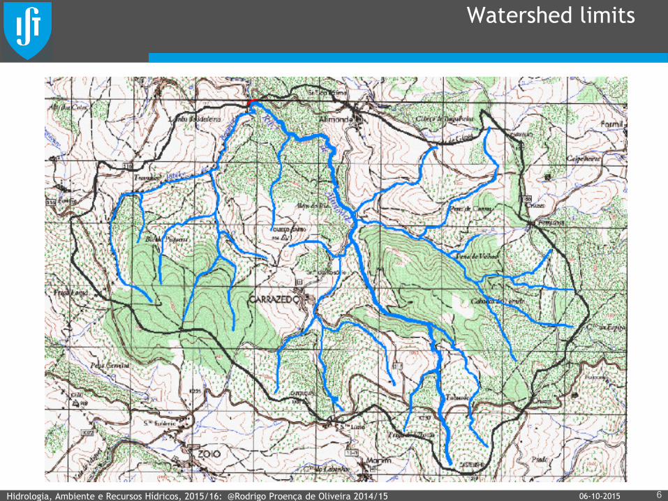
Watershed limits
Hidrologia, Ambiente e Recursos Hídricos, 2015/16: @Rodrigo Proença de Oliveira 2014/15 6 06-10-2015
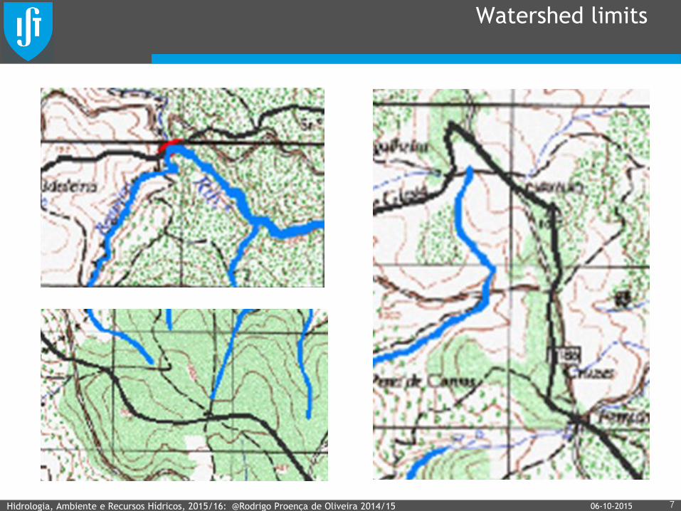
Watershed limits
Hidrologia, Ambiente e Recursos Hídricos, 2015/16: @Rodrigo Proença de Oliveira 2014/15 7 06-10-2015
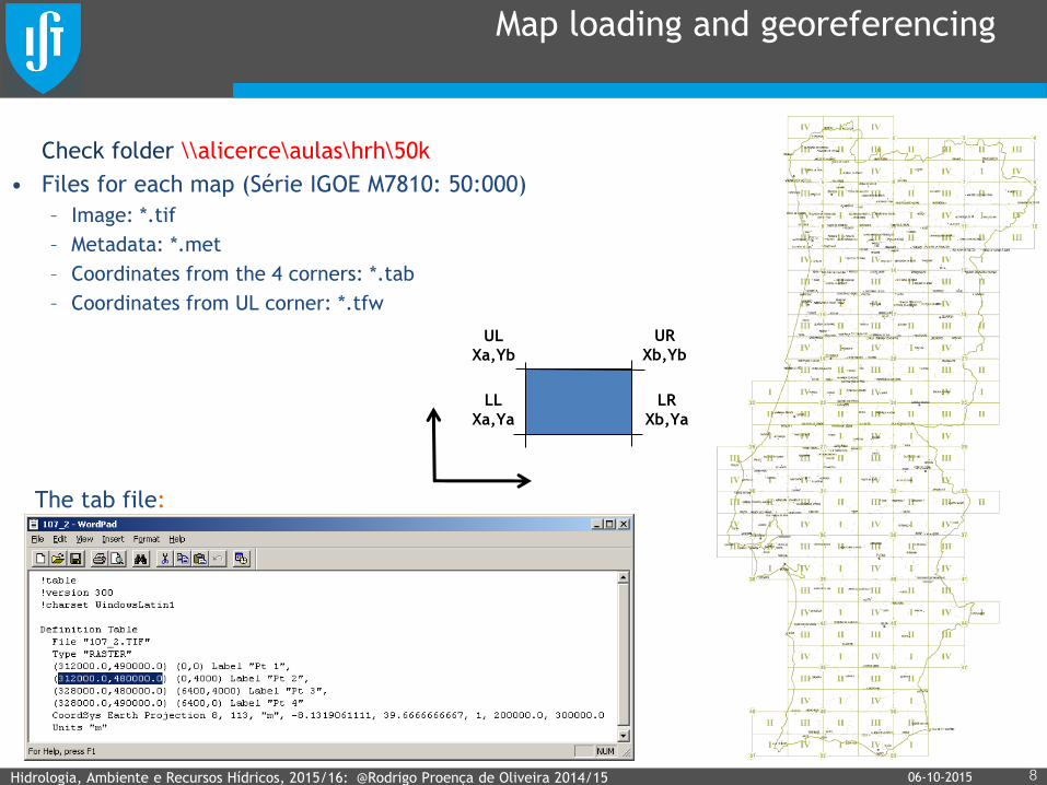
Map loading and georeferencing
Hidrologia, Ambiente e Recursos Hídricos, 2015/16: @Rodrigo Proença de Oliveira 2014/15 8
Check folder \\alicerce\aulas\hrh\50k
• Files for each map (Série IGOE M7810: 50:000)
– Image: *.tif
– Metadata: *.met
– Coordinates from the 4 corners: *.tab
– Coordinates from UL corner: *.tfw
UL
Xa,Yb
LL
Xa,Ya
LR
Xb,Ya
UR
Xb,Yb
The tab file:
06-10-2015
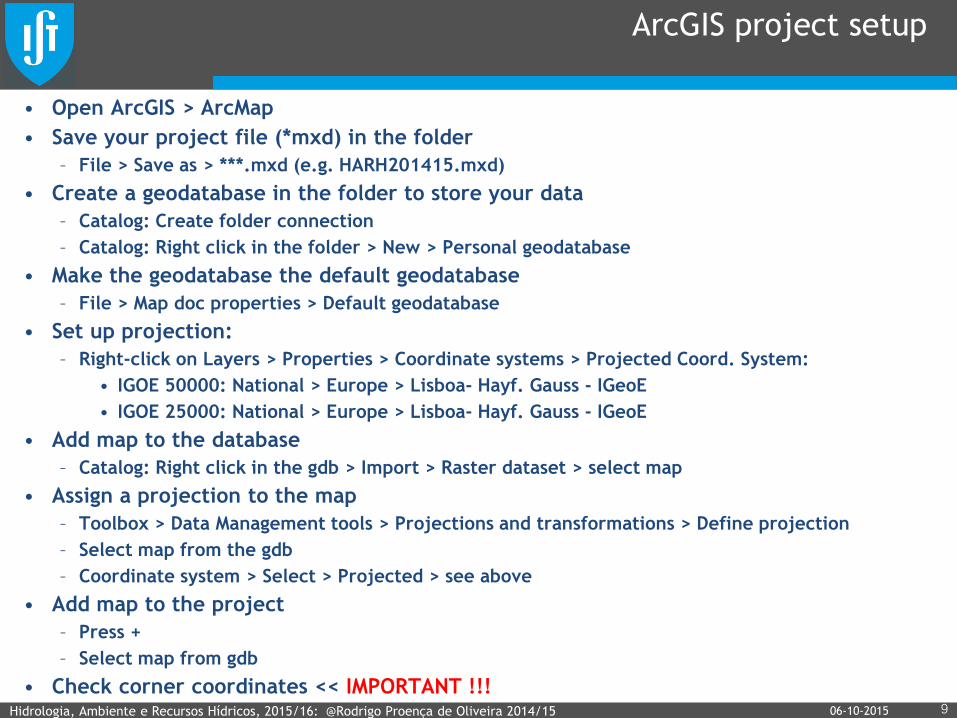
ArcGIS project setup
• Open ArcGIS > ArcMap
• Save your project file (*mxd) in the folder
– File > Save as > ***.mxd (e.g. HARH201415.mxd)
• Create a geodatabase in the folder to store your data
– Catalog: Create folder connection
– Catalog: Right click in the folder > New > Personal geodatabase
• Make the geodatabase the default geodatabase
– File > Map doc properties > Default geodatabase
• Set up projection:
– Right-click on Layers > Properties > Coordinate systems > Projected Coord. System:
• IGOE 50000: National > Europe > Lisboa- Hayf. Gauss - IGeoE
• IGOE 25000: National > Europe > Lisboa- Hayf. Gauss - IGeoE
• Add map to the database
– Catalog: Right click in the gdb > Import > Raster dataset > select map
• Assign a projection to the map
– Toolbox > Data Management tools > Projections and transformations > Define projection
– Select map from the gdb
– Coordinate system > Select > Projected > see above
• Add map to the project
– Press +
– Select map from gdb
• Check corner coordinates << IMPORTANT !!!
Hidrologia, Ambiente e Recursos Hídricos, 2015/16: @Rodrigo Proença de Oliveira 2014/15 9 06-10-2015
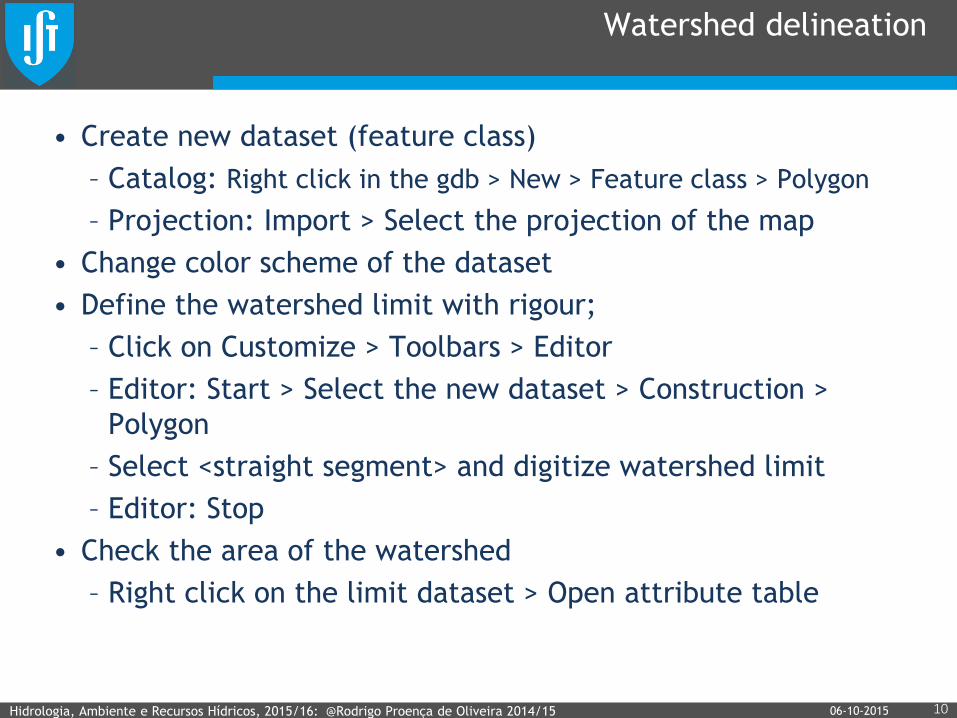
Watershed delineation
• Create new dataset (feature class)
– Catalog: Right click in the gdb > New > Feature class > Polygon
– Projection: Import > Select the projection of the map
• Change color scheme of the dataset
• Define the watershed limit with rigour;
– Click on Customize > Toolbars > Editor
– Editor: Start > Select the new dataset > Construction >
Polygon
– Select <straight segment> and digitize watershed limit
– Editor: Stop
• Check the area of the watershed
– Right click on the limit dataset > Open attribute table
Hidrologia, Ambiente e Recursos Hídricos, 2015/16: @Rodrigo Proença de Oliveira 2014/15 10 06-10-2015
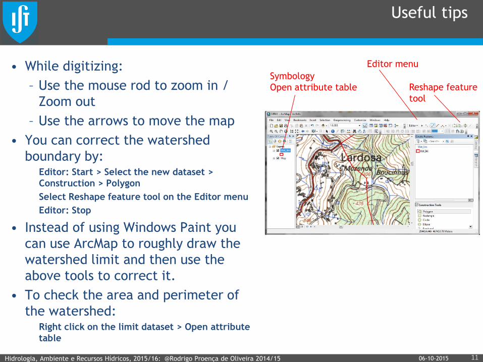
Useful tips
• While digitizing:
– Use the mouse rod to zoom in /
Zoom out
– Use the arrows to move the map
• You can correct the watershed
boundary by: Editor: Start > Select the new dataset >
Construction > Polygon
Select Reshape feature tool on the Editor menu
Editor: Stop
• Instead of using Windows Paint you
can use ArcMap to roughly draw the
watershed limit and then use the
above tools to correct it.
• To check the area and perimeter of
the watershed: Right click on the limit dataset > Open attribute
table
Hidrologia, Ambiente e Recursos Hídricos, 2015/16: @Rodrigo Proença de Oliveira 2014/15 11 06-10-2015
Symbology
Open attribute table Reshape feature
tool
Editor menu
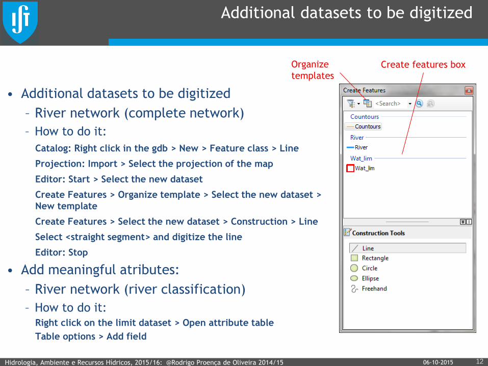
Additional datasets to be digitized
• Additional datasets to be digitized
– River network (complete network)
– How to do it:
Catalog: Right click in the gdb > New > Feature class > Line
Projection: Import > Select the projection of the map
Editor: Start > Select the new dataset
Create Features > Organize template > Select the new dataset >
New template
Create Features > Select the new dataset > Construction > Line
Select <straight segment> and digitize the line
Editor: Stop
• Add meaningful atributes:
– River network (river classification)
– How to do it: Right click on the limit dataset > Open attribute table
Table options > Add field
Hidrologia, Ambiente e Recursos Hídricos, 2015/16: @Rodrigo Proença de Oliveira 2014/15 12 06-10-2015
Organize
templates Create features box
Watershed characterization
Part 1
Shape characterization
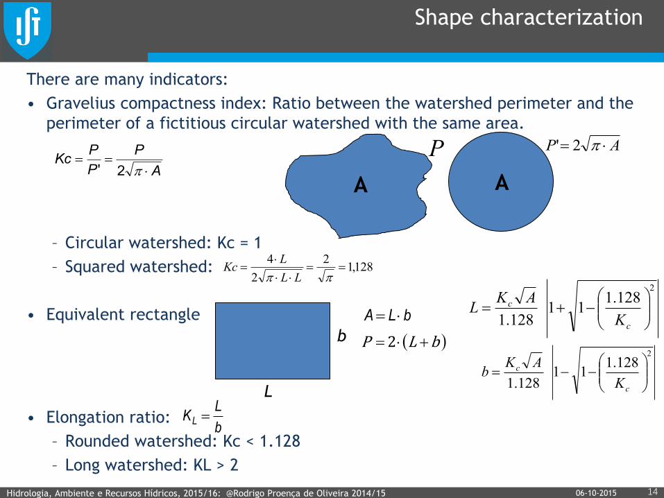
There are many indicators:
• Gravelius compactness index: Ratio between the watershed perimeter and the
perimeter of a fictitious circular watershed with the same area.
– Circular watershed: Kc = 1
– Squared watershed:
• Equivalent rectangle
• Elongation ratio:
– Rounded watershed: Kc < 1.128
– Long watershed: KL > 2
Hidrologia, Ambiente e Recursos Hídricos, 2015/16: @Rodrigo Proença de Oliveira 2014/15 14 06-10-2015
A
P
P
PKc
2'
A A
AP 2'P
128,12
2
4
LL
LKc
bLA
bLP 2
L
b
2
128.111
128.1
c
c
K
AKL
2
128.111
128.1
c
c
K
AKb
b
LKL
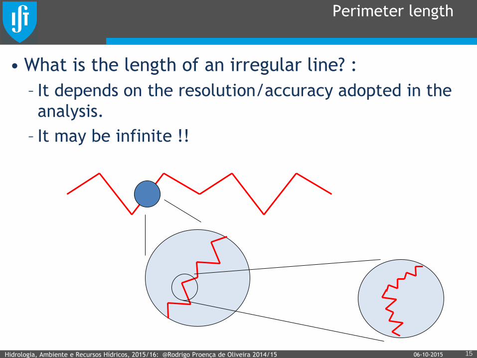
Perimeter length
• What is the length of an irregular line? :
– It depends on the resolution/accuracy adopted in the
analysis.
– It may be infinite !!
Hidrologia, Ambiente e Recursos Hídricos, 2015/16: @Rodrigo Proença de Oliveira 2014/15 15 06-10-2015
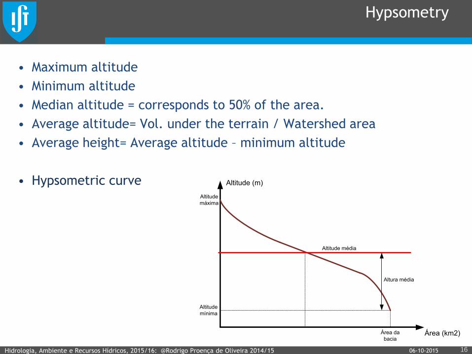
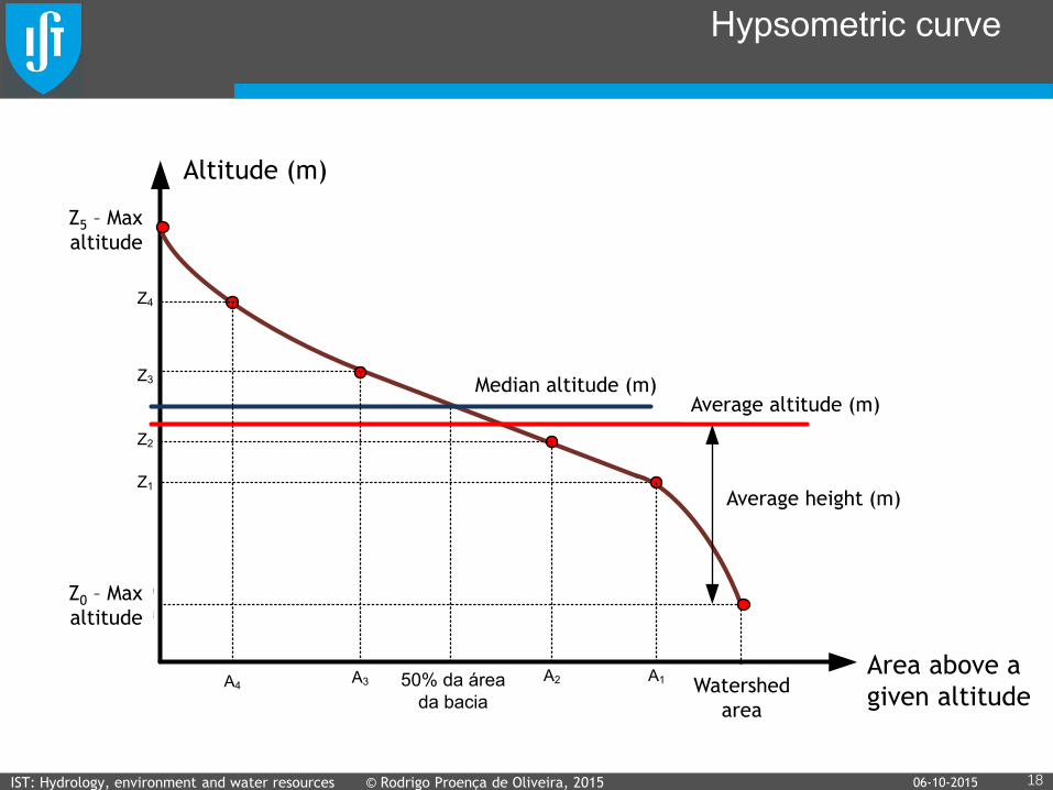
Hypsometry
• Maximum altitude
• Minimum altitude
• Median altitude = corresponds to 50% of the area.
• Average altitude= Vol. under the terrain / Watershed area
• Average height= Average altitude – minimum altitude
• Hypsometric curve
Hidrologia, Ambiente e Recursos Hídricos, 2015/16: @Rodrigo Proença de Oliveira 2014/15 16
Área (km2)
Altitude (m)
Altitude média
Altitude
máxima
Altitude
mínima
Área da
bacia
Altura média
06-10-2015
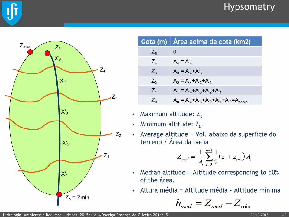
Hypsometry
• Maximum altitude: Z5
• Minimum altitude: Z0
• Average altitude = Vol. abaixo da superficie do
terreno / Área da bacia
• Median altitude = Altitude corresponding to 50%
of the área.
• Altura média = Altitude média - Altitude mínima
Hidrologia, Ambiente e Recursos Hídricos, 2015/16: @Rodrigo Proença de Oliveira 2014/15 17
1
0
'
12
11 n
i
iii
t
med AzzA
Z
Cota (m) Área acima da cota (km2)
Z5 0
Z4 A4 = A’4
Z3 A3 = A’4+A’3
Z2 A2 = A’4+A’3+A’2
Z1 A1 = A’4+A’3+A’2+A’1
Z0 A0 = A’4+A’3+A’2+A’1+A’0=Abacia
minZZh medmed
06-10-2015
Zo = Zmin
Z1
Z2
Z3
Z4
Z5
X’2
X’3
X’4
X’5
X’1
Zmax
Hypsometric curve
IST: Hydrology, environment and water resources © Rodrigo Proença de Oliveira, 2015 18
Área acima da
cota (km2)
Altitude/Cota (m)
Altitude média
Z5 = Altitude
máxima
Z0 = Altitude
mínima
Área da
bacia
Altura média
50% da área
da bacia
Altitude mediana
Z1
Z2
Z3
Z4
A1A2A3A4
Area above a
given altitude
Altitude (m)
Median altitude (m) Average altitude (m)
Average height (m)
Watershed
area
Z5 – Max
altitude
Z0 – Max
altitude
06-10-2015
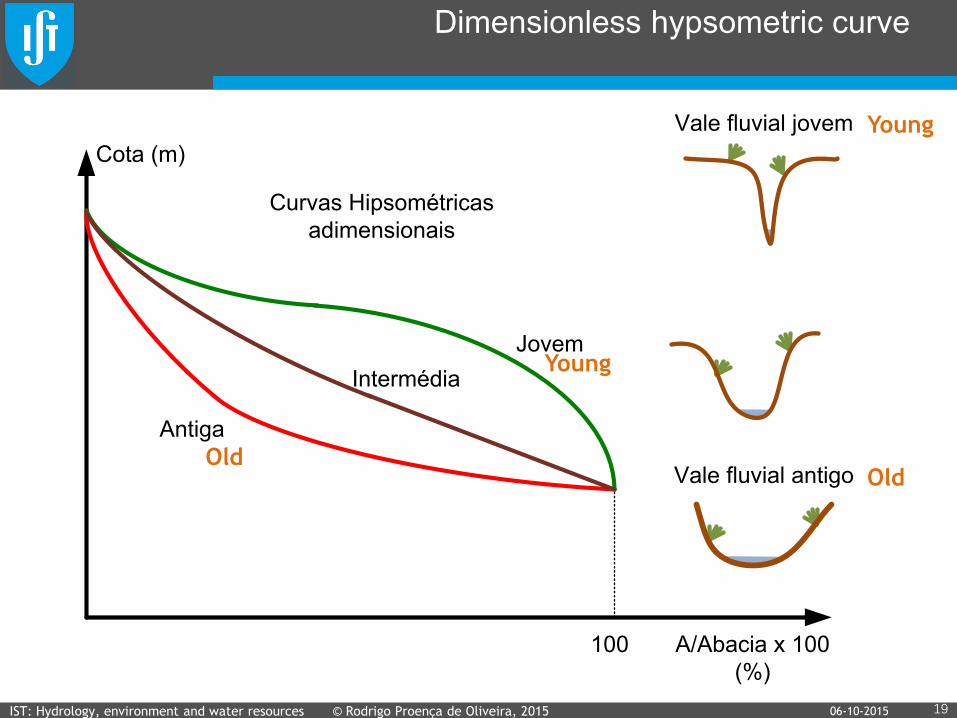
Dimensionless hypsometric curve
IST: Hydrology, environment and water resources © Rodrigo Proença de Oliveira, 2015 19 06-10-2015
A/Abacia x 100
(%)
Cota (m)
Curvas Hipsométricas
adimensionais
Jovem
Antiga
Intermédia
100
Vale fluvial jovem
Vale fluvial antigo
Young
Old
Young
Old
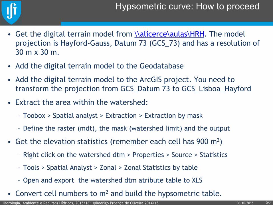
Hypsometric curve: How to proceed
• Get the digital terrain model from \\alicerce\aulas\HRH. The model
projection is Hayford-Gauss, Datum 73 (GCS_73) and has a resolution of
30 m x 30 m.
• Add the digital terrain model to the Geodatabase
• Add the digital terrain model to the ArcGIS project. You need to
transform the projection from GCS_Datum 73 to GCS_Lisboa_Hayford
• Extract the area within the watershed:
– Toobox > Spatial analyst > Extraction > Extraction by mask
– Define the raster (mdt), the mask (watershed limit) and the output
• Get the elevation statistics (remember each cell has 900 m2)
– Right click on the watershed dtm > Properties > Source > Statistics
– Tools > Spatial Analyst > Zonal > Zonal Statistics by table
– Open and export the watershed dtm atribute table to XLS
• Convert cell numbers to m2 and build the hypsometric table.
Hidrologia, Ambiente e Recursos Hídricos, 2015/16: @Rodrigo Proença de Oliveira 2014/15 20 06-10-2015
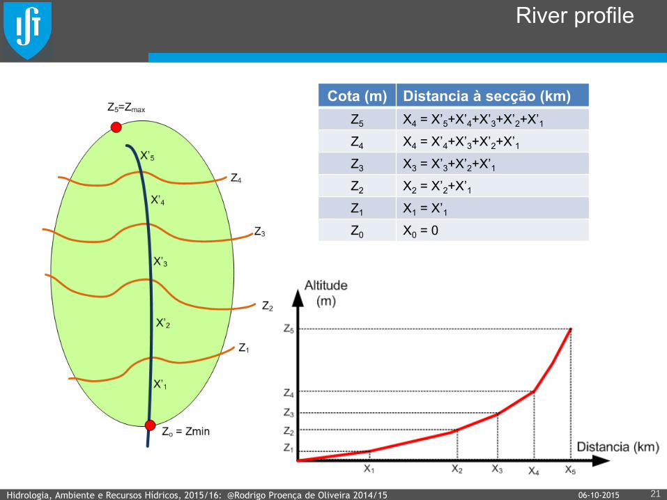
River profile
Hidrologia, Ambiente e Recursos Hídricos, 2015/16: @Rodrigo Proença de Oliveira 2014/15 21
Cota (m) Distancia à secção (km)
Z5 X4 = X’5+X’4+X’3+X’2+X’1
Z4 X4 = X’4+X’3+X’2+X’1
Z3 X3 = X’3+X’2+X’1
Z2 X2 = X’2+X’1
Z1 X1 = X’1
Z0 X0 = 0
06-10-2015
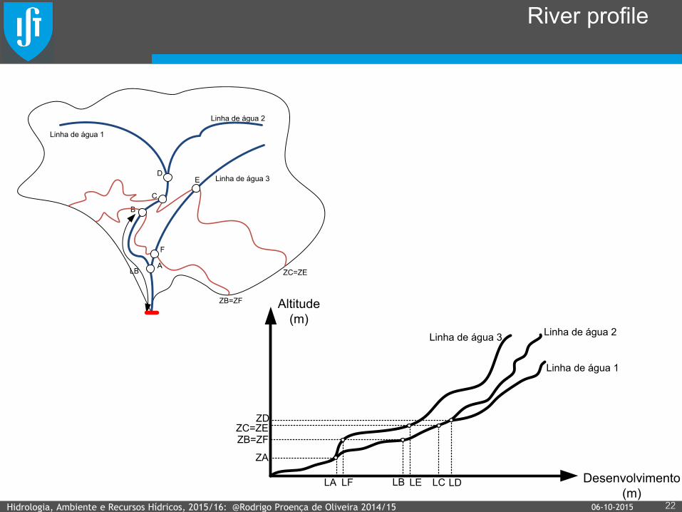
River profile
Hidrologia, Ambiente e Recursos Hídricos, 2015/16: @Rodrigo Proença de Oliveira 2014/15 22
A
B
C
D
Linha de água 1
Linha de água 2
Linha de água 3
LB
ZB=ZF
ZC=ZE
E
F
Altitude
(m)
Desenvolvimento
(m)
Linha de água 1
Linha de água 2Linha de água 3
ZA
LA
ZC=ZE
LB LC
ZB=ZF
ZD
LDLELF
06-10-2015
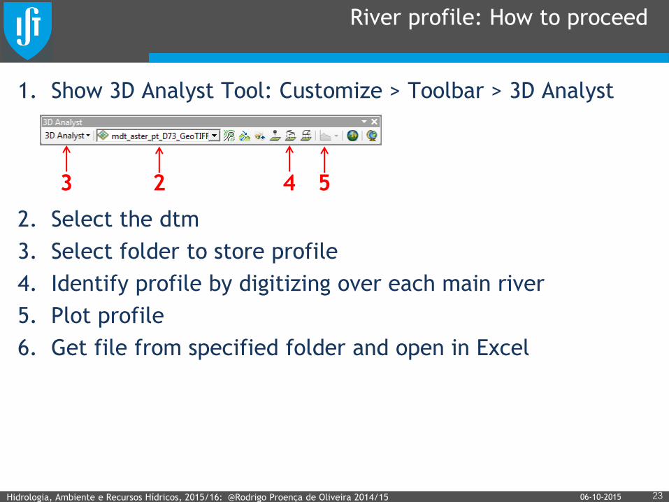
River profile: How to proceed
1. Show 3D Analyst Tool: Customize > Toolbar > 3D Analyst
2. Select the dtm
3. Select folder to store profile
4. Identify profile by digitizing over each main river
5. Plot profile
6. Get file from specified folder and open in Excel
Hidrologia, Ambiente e Recursos Hídricos, 2015/16: @Rodrigo Proença de Oliveira 2014/15 23 06-10-2015
2 3 4 5
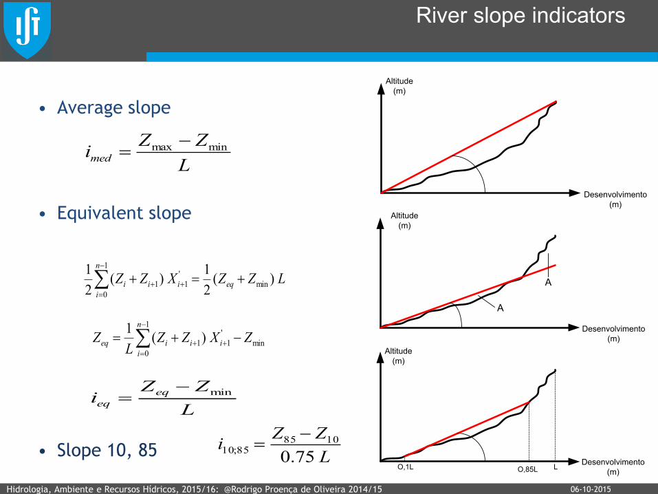
River slope indicators
• Average slope
• Equivalent slope
• Slope 10, 85
Hidrologia, Ambiente e Recursos Hídricos, 2015/16: @Rodrigo Proença de Oliveira 2014/15 24
Altitude
(m)
Desenvolvimento
(m)
Altitude
(m)
Desenvolvimento
(m)
Altitude
(m)
Desenvolvimento
(m)
A
A
O,1L O,85L L
L
ZZimed
minmax
LZZXZZ eqi
n
i
ii )(2
1)(
2
1min
'
1
1
0
1
min
1
0
'
11)(1
ZXZZL
Zn
i
iiieq
L
ZZi
eq
eq
min
L
ZZi
75.0
108585;10
06-10-2015
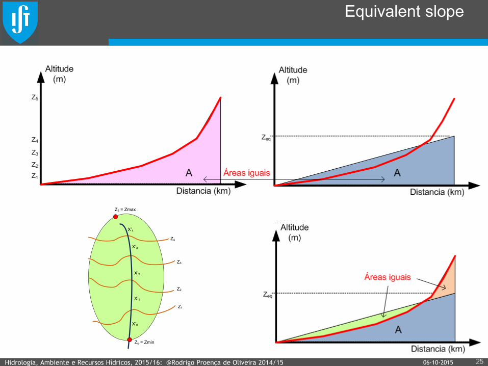
Equivalent slope
Hidrologia, Ambiente e Recursos Hídricos, 2015/16: @Rodrigo Proença de Oliveira 2014/15 25
Zo = Zmin
Z1
Z2
Z3
Z4
Z5 = Zmax
X’1
X’2
X’3
X’4
X’0
06-10-2015
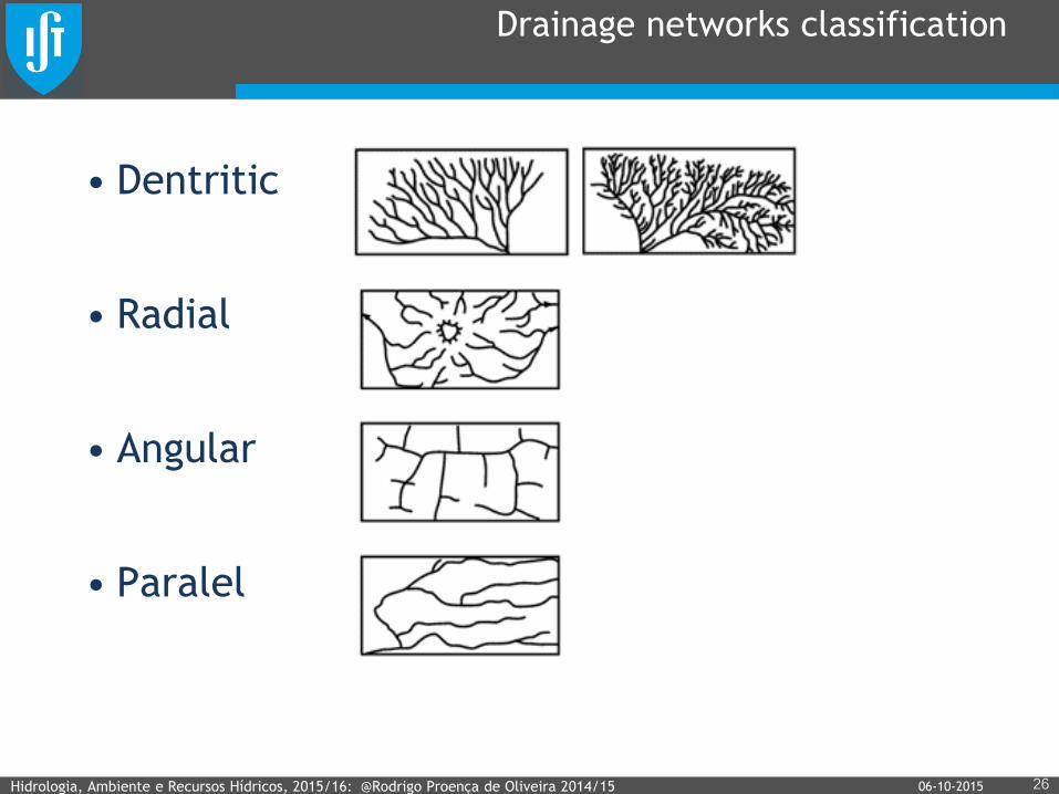
Drainage networks classification
• Dentritic
• Radial
• Angular
• Paralel
Hidrologia, Ambiente e Recursos Hídricos, 2015/16: @Rodrigo Proença de Oliveira 2014/15 26 06-10-2015
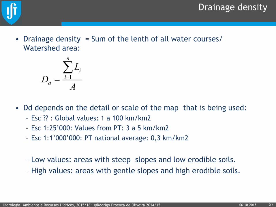
Drainage density
• Drainage density = Sum of the lenth of all water courses/
Watershed area:
• Dd depends on the detail or scale of the map that is being used:
– Esc ?? : Global values: 1 a 100 km/km2
– Esc 1:25’000: Values from PT: 3 a 5 km/km2
– Esc 1:1’000’000: PT national average: 0,3 km/km2
– Low values: areas with steep slopes and low erodible soils.
– High values: areas with gentle slopes and high erodible soils.
Hidrologia, Ambiente e Recursos Hídricos, 2015/16: @Rodrigo Proença de Oliveira 2014/15 27 06-10-2015
A
L
D
n
i
i
d
1
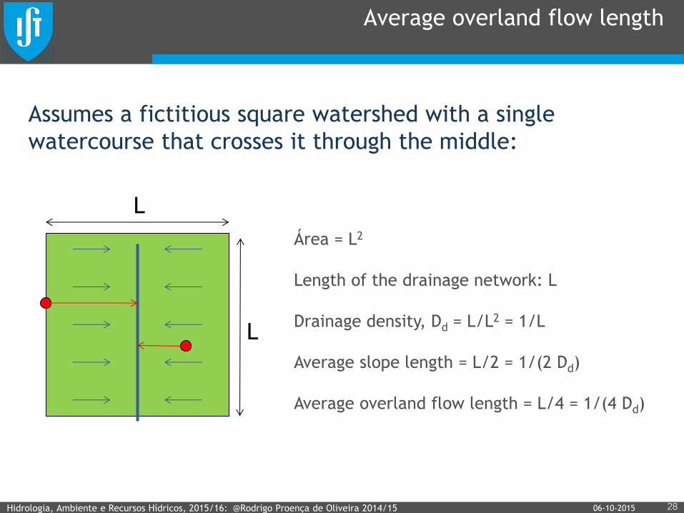
Average overland flow length
Assumes a fictitious square watershed with a single
watercourse that crosses it through the middle:
Hidrologia, Ambiente e Recursos Hídricos, 2015/16: @Rodrigo Proença de Oliveira 2014/15 28 06-10-2015
L
L
Área = L2
Length of the drainage network: L
Drainage density, Dd = L/L2 = 1/L
Average slope length = L/2 = 1/(2 Dd)
Average overland flow length = L/4 = 1/(4 Dd)
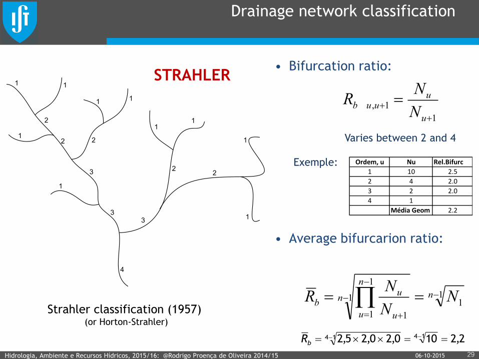
Drainage network classification
• Bifurcation ratio:
• Average bifurcarion ratio:
Hidrologia, Ambiente e Recursos Hídricos, 2015/16: @Rodrigo Proença de Oliveira 2014/15 29
1
1
1
1
1
1
1
1
1
2
3 22
2
1
2
33
4
Strahler classification (1957) (or Horton-Strahler)
11
1
1
1 1
nn
n
u u
ub N
N
NR
1
1,
u
uuub
N
NR
Ordem, u Nu Rel.Bifurc
1 10 2.5
2 4 2.0
3 2 2.0
4 1
Média Geom 2.2
2,2100,20,25,2 1414 bR
Varies between 2 and 4
Exemple:
06-10-2015
STRAHLER
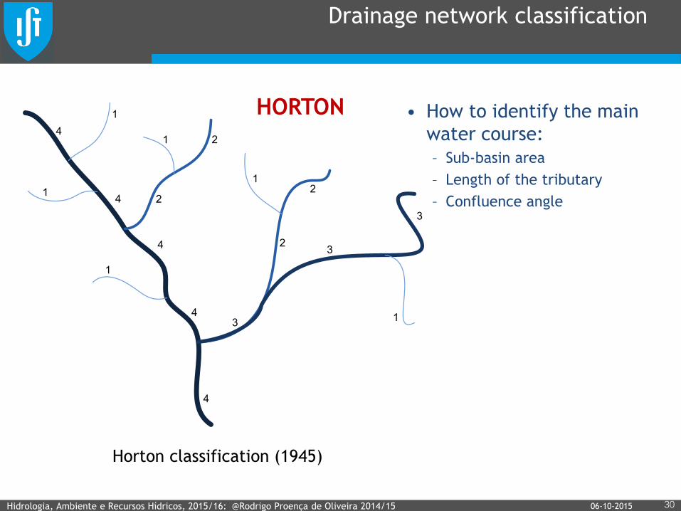
Drainage network classification
Hidrologia, Ambiente e Recursos Hídricos, 2015/16: @Rodrigo Proença de Oliveira 2014/15 30
1
1
1
1
1
1
2
2
3
4
4
4
4
4
3
3
2
2
Horton classification (1945)
• How to identify the main
water course:
– Sub-basin area
– Length of the tributary
– Confluence angle
06-10-2015
HORTON
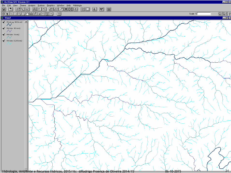
Hidrologia, Ambiente e Recursos Hídricos, 2015/16: @Rodrigo Proença de Oliveira 2014/15 31 06-10-2015
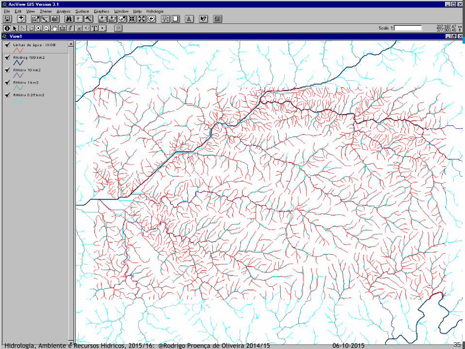
Hidrologia, Ambiente e Recursos Hídricos, 2015/16: @Rodrigo Proença de Oliveira 2014/15 32 06-10-2015
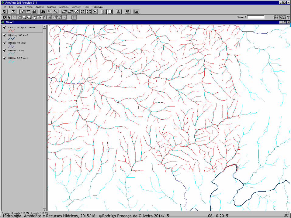
06-10-2015 33 Hidrologia, Ambiente e Recursos Hídricos, 2015/16: @Rodrigo Proença de Oliveira 2014/15 06-10-2015
06-10-2015 34 Hidrologia, Ambiente e Recursos Hídricos, 2015/16: @Rodrigo Proença de Oliveira 2014/15 06-10-2015
06-10-2015 35 Hidrologia, Ambiente e Recursos Hídricos, 2015/16: @Rodrigo Proença de Oliveira 2014/15 06-10-2015
06-10-2015 36 Hidrologia, Ambiente e Recursos Hídricos, 2015/16: @Rodrigo Proença de Oliveira 2014/15 06-10-2015
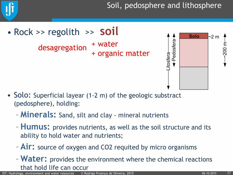
Soil, pedosphere and lithosphere
• Rock >> regolith >> soil
• Solo: Superficial layear (1-2 m) of the geologic substract
(pedosphere), holding:
– Minerals: Sand, silt and clay - mineral nutrients
– Humus: provides nutrients, as well as the soil structure and its
ability to hold water and nutrients;
– Air: source of oxygen and CO2 requited by micro organisms
– Water: provides the environment where the chemical reactions
that hold life can occur
IST: Hydrology, environment and water resources © Rodrigo Proença de Oliveira, 2015 37
desagregation + water
+ organic matter
Solo
Lito
sfe
ra
Pe
do
sfe
ra
~2
00
m
~2 m
06-10-2015
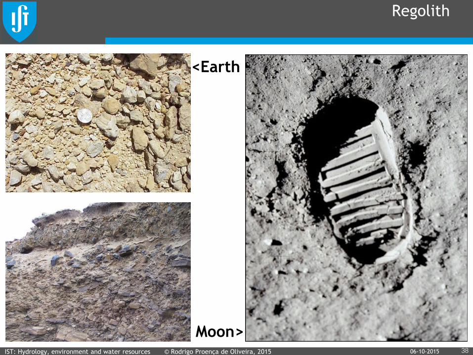
Regolith
IST: Hydrology, environment and water resources © Rodrigo Proença de Oliveira, 2015 38
<Earth
Moon> 06-10-2015
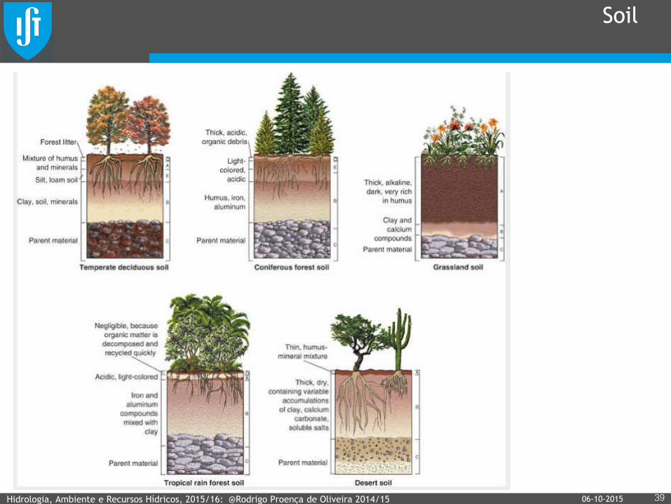
Soil
Hidrologia, Ambiente e Recursos Hídricos, 2015/16: @Rodrigo Proença de Oliveira 2014/15 39 06-10-2015
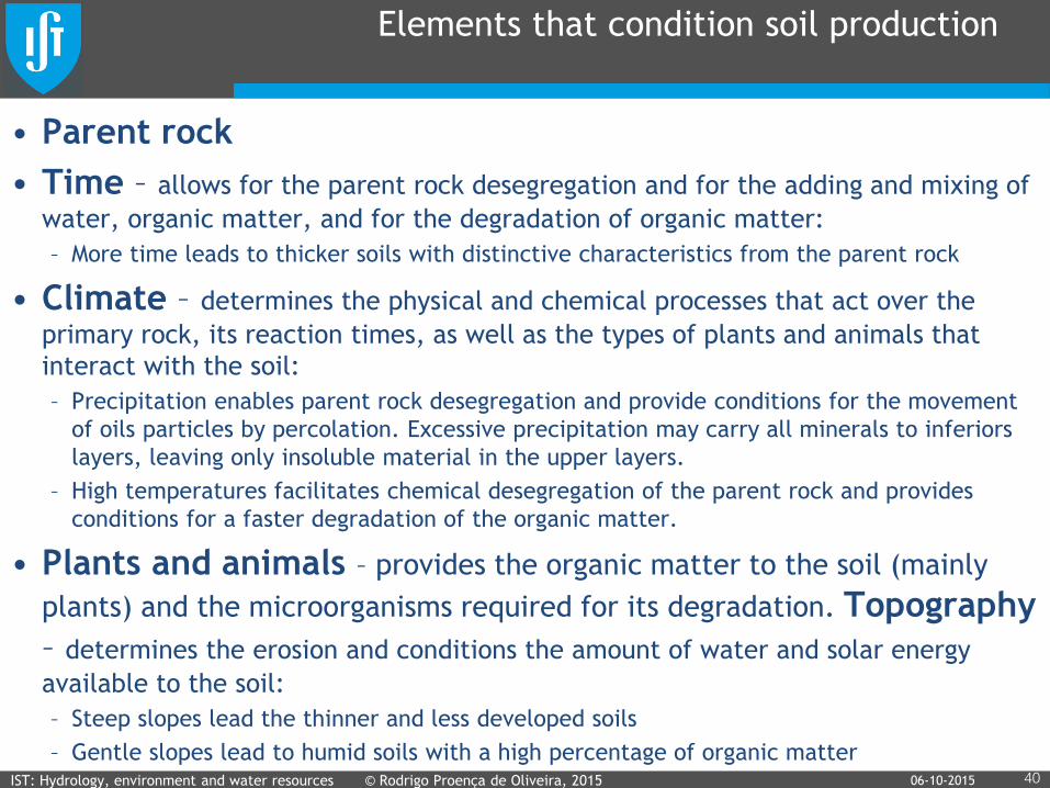
Elements that condition soil production
• Parent rock
• Time – allows for the parent rock desegregation and for the adding and mixing of
water, organic matter, and for the degradation of organic matter:
– More time leads to thicker soils with distinctive characteristics from the parent rock
• Climate – determines the physical and chemical processes that act over the
primary rock, its reaction times, as well as the types of plants and animals that
interact with the soil:
– Precipitation enables parent rock desegregation and provide conditions for the movement
of oils particles by percolation. Excessive precipitation may carry all minerals to inferiors
layers, leaving only insoluble material in the upper layers.
– High temperatures facilitates chemical desegregation of the parent rock and provides
conditions for a faster degradation of the organic matter.
• Plants and animals – provides the organic matter to the soil (mainly
plants) and the microorganisms required for its degradation. Topography
– determines the erosion and conditions the amount of water and solar energy
available to the soil:
– Steep slopes lead the thinner and less developed soils
– Gentle slopes lead to humid soils with a high percentage of organic matter
IST: Hydrology, environment and water resources © Rodrigo Proença de Oliveira, 2015 40 06-10-2015
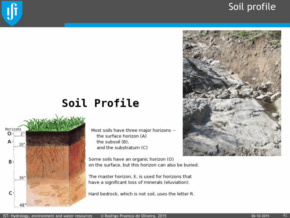
Soil profile
IST: Hydrology, environment and water resources © Rodrigo Proença de Oliveira, 2015 41 06-10-2015
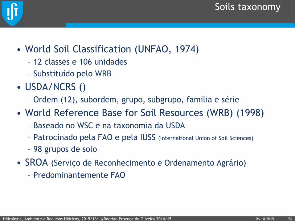
Soils taxonomy
• World Soil Classification (UNFAO, 1974)
– 12 classes e 106 unidades
– Substituído pelo WRB
• USDA/NCRS ()
– Ordem (12), subordem, grupo, subgrupo, família e série
• World Reference Base for Soil Resources (WRB) (1998)
– Baseado no WSC e na taxonomia da USDA
– Patrocinado pela FAO e pela IUSS (International Union of Soil Sciences)
– 98 grupos de solo
• SROA (Serviço de Reconhecimento e Ordenamento Agrário)
– Predominantemente FAO
Hidrologia, Ambiente e Recursos Hídricos, 2015/16: @Rodrigo Proença de Oliveira 2014/15 42 06-10-2015
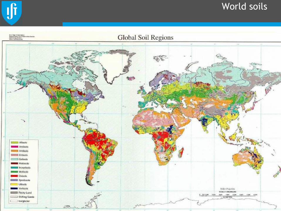
World soils
Hidrologia, Ambiente e Recursos Hídricos, 2015/16: @Rodrigo Proença de Oliveira 2014/15 43 06-10-2015
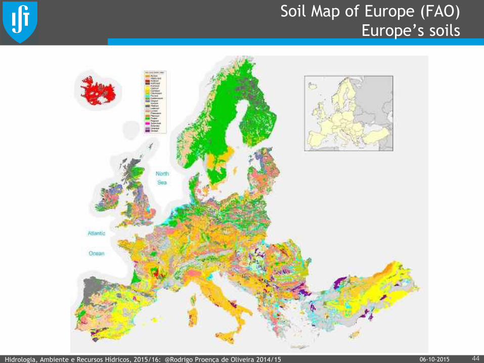
Soil Map of Europe (FAO)
Europe’s soils
Hidrologia, Ambiente e Recursos Hídricos, 2015/16: @Rodrigo Proença de Oliveira 2014/15 44 06-10-2015
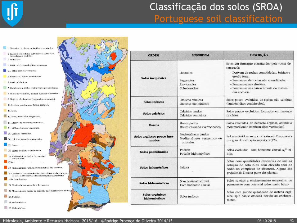
Classificação dos solos (SROA)
Portuguese soil classification
Hidrologia, Ambiente e Recursos Hídricos, 2015/16: @Rodrigo Proença de Oliveira 2014/15 45 06-10-2015
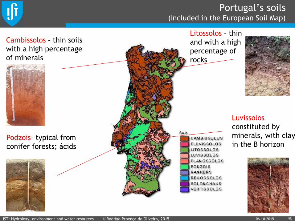
Portugal’s soils (included in the European Soil Map)
46 06-10-2015
Cambissolos – thin soils
with a high percentage
of minerals
Litossolos – thin
and with a high
percentage of
rocks
Podzois– typical from
conifer forests; ácids
Luvissolos
constituted by
minerals, with clay
in the B horizon
IST: Hydrology, environment and water resources © Rodrigo Proença de Oliveira, 2015
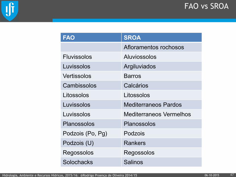
FAO vs SROA
Hidrologia, Ambiente e Recursos Hídricos, 2015/16: @Rodrigo Proença de Oliveira 2014/15 47
FAO SROA
Afloramentos rochosos
Fluvissolos Aluviossolos
Luvissolos Argiluviados
Vertissolos Barros
Cambissolos Calcários
Litossolos Litossolos
Luvissolos Mediterraneos Pardos
Luvissolos Mediterraneos Vermelhos
Planossolos Planossolos
Podzois (Po, Pg) Podzois
Podzois (U) Rankers
Regossolos Regossolos
Solochacks Salinos
06-10-2015
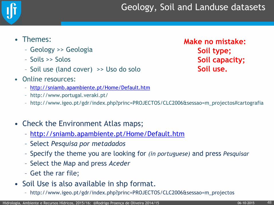
Geology, Soil and Landuse datasets
• Themes:
– Geology >> Geologia
– Soils >> Solos
– Soil use (land cover) >> Uso do solo
• Online resources: – http://sniamb.apambiente.pt/Home/Default.htm
– http://www.portugal.veraki.pt/
– http://www.igeo.pt/gdr/index.php?princ=PROJECTOS/CLC2006&sessao=m_projectos#cartografia
• Check the Environment Atlas maps;
– http://sniamb.apambiente.pt/Home/Default.htm
– Select Pesquisa por metadados
– Specify the theme you are looking for (in portuguese) and press Pesquisar
– Select the Map and press Aceder
– Get the rar file;
• Soil Use is also available in shp format. – http://www.igeo.pt/gdr/index.php?princ=PROJECTOS/CLC2006&sessao=m_projectos
Hidrologia, Ambiente e Recursos Hídricos, 2015/16: @Rodrigo Proença de Oliveira 2014/15 48 06-10-2015
Make no mistake:
Soil type;
Soil capacity;
Soil use.
Climatic and hydrological
charaterization
Part 2
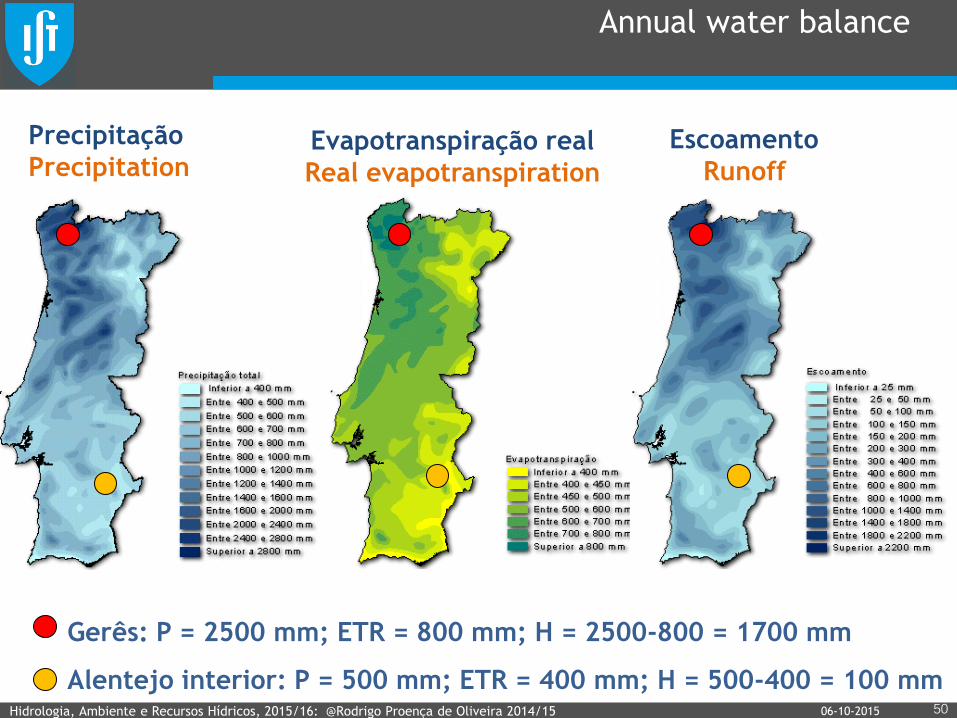
Annual water balance
Hidrologia, Ambiente e Recursos Hídricos, 2015/16: @Rodrigo Proença de Oliveira 2014/15
Precipitação
Precipitation Evapotranspiração real
Real evapotranspiration
Escoamento
Runoff
50
Gerês: P = 2500 mm; ETR = 800 mm; H = 2500-800 = 1700 mm
Alentejo interior: P = 500 mm; ETR = 400 mm; H = 500-400 = 100 mm 06-10-2015
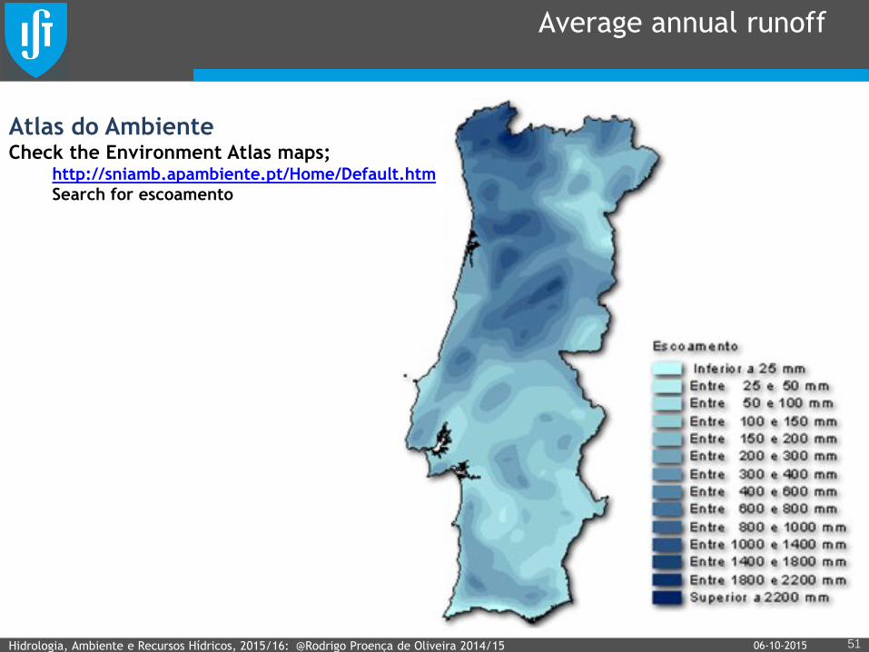
Average annual runoff
Hidrologia, Ambiente e Recursos Hídricos, 2015/16: @Rodrigo Proença de Oliveira 2014/15 51 06-10-2015
Atlas do Ambiente Check the Environment Atlas maps;
http://sniamb.apambiente.pt/Home/Default.htm
Search for escoamento
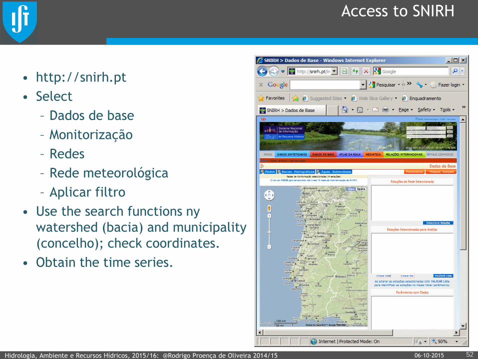
Access to SNIRH
• http://snirh.pt
• Select
– Dados de base
– Monitorização
– Redes
– Rede meteorológica
– Aplicar filtro
• Use the search functions ny
watershed (bacia) and municipality
(concelho); check coordinates.
• Obtain the time series.
Hidrologia, Ambiente e Recursos Hídricos, 2015/16: @Rodrigo Proença de Oliveira 2014/15 52 06-10-2015
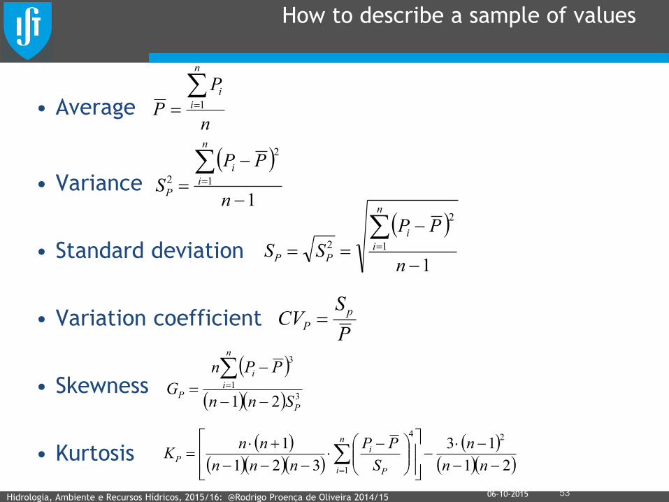
How to describe a sample of values
• Average
• Variance
• Standard deviation
• Variation coefficient
• Skewness
• Kurtosis
Hidrologia, Ambiente e Recursos Hídricos, 2015/16: @Rodrigo Proença de Oliveira 2014/15 53
n
P
P
n
i
i 1
11
2
2
n
PP
S
n
i
i
P
11
2
2
n
PP
SS
n
i
i
PP
P
SCV
p
P
3
1
3
21 P
n
i
i
PSnn
PPn
G
21
13
321
12
1
4
nn
n
S
PP
nnn
nnK
n
i P
iP
06-10-2015
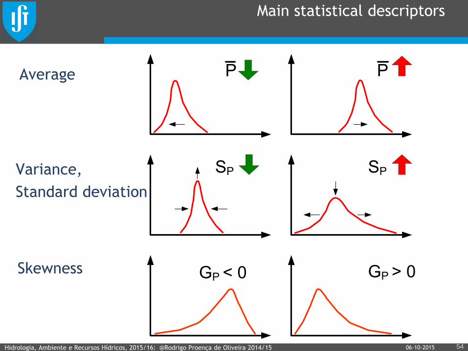
Main statistical descriptors
Hidrologia, Ambiente e Recursos Hídricos, 2015/16: @Rodrigo Proença de Oliveira 2014/15 54
P
SP
GP < 0
P
SP
GP > 0
Average
Variance,
Standard deviation
Skewness
06-10-2015
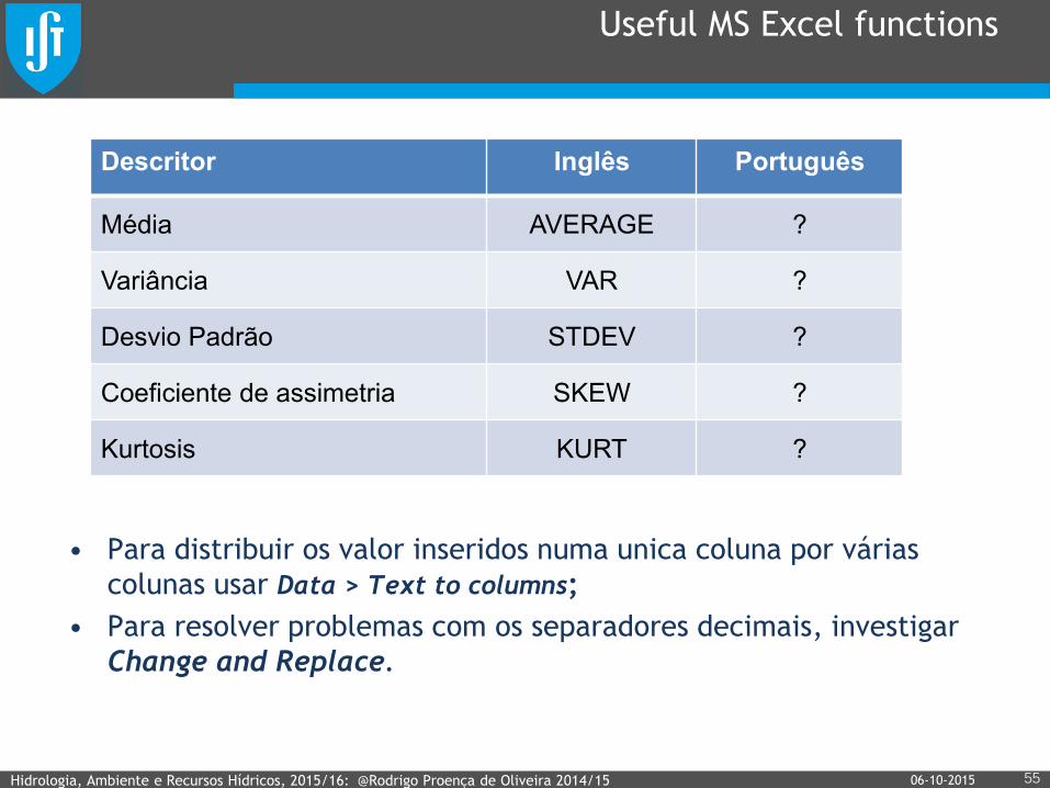
Useful MS Excel functions
• Para distribuir os valor inseridos numa unica coluna por várias
colunas usar Data > Text to columns;
• Para resolver problemas com os separadores decimais, investigar
Change and Replace.
Hidrologia, Ambiente e Recursos Hídricos, 2015/16: @Rodrigo Proença de Oliveira 2014/15 55
Descritor Inglês Português
Média AVERAGE ?
Variância VAR ?
Desvio Padrão STDEV ?
Coeficiente de assimetria SKEW ?
Kurtosis KURT ?
06-10-2015
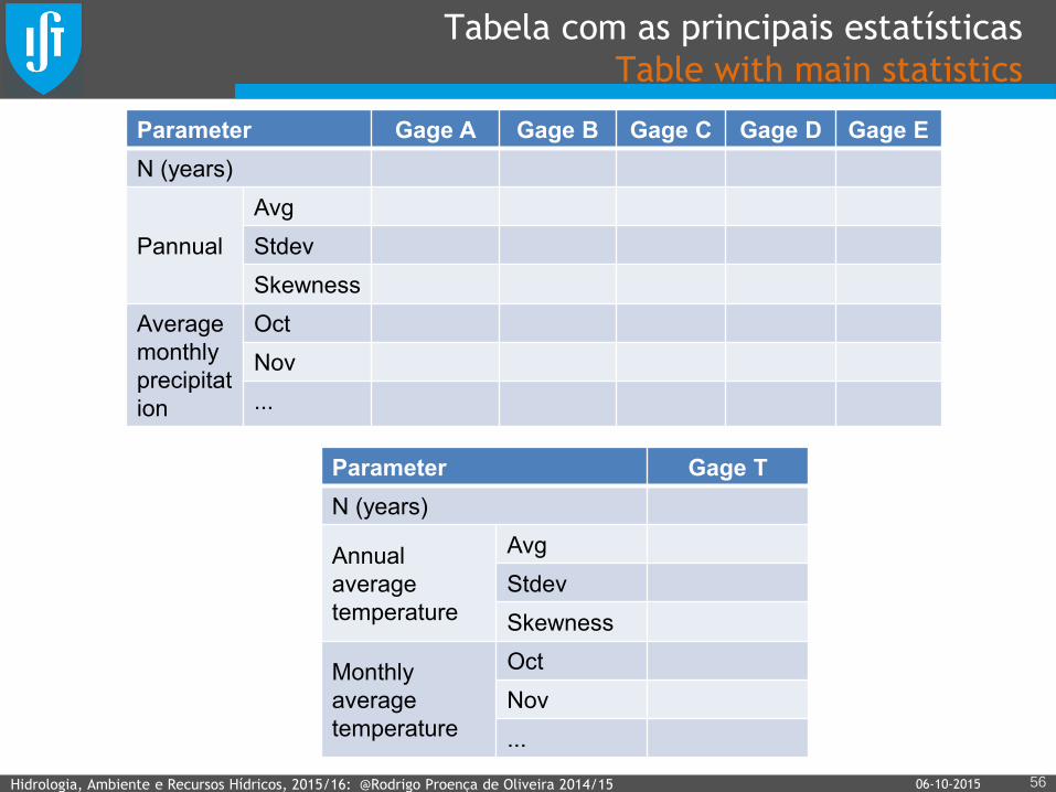
Tabela com as principais estatísticas
Table with main statistics
Hidrologia, Ambiente e Recursos Hídricos, 2015/16: @Rodrigo Proença de Oliveira 2014/15 56 06-10-2015
Parameter Gage A Gage B Gage C Gage D Gage E
N (years)
Pannual
Avg
Stdev
Skewness
Average
monthly
precipitat
ion
Oct
Nov
...
Parameter Gage T
N (years)
Annual
average
temperature
Avg
Stdev
Skewness
Monthly
average
temperature
Oct
Nov
...
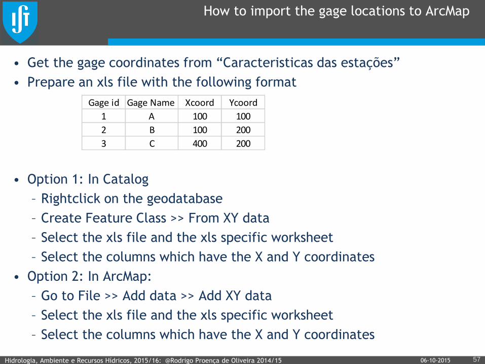
How to import the gage locations to ArcMap
• Get the gage coordinates from “Caracteristicas das estações”
• Prepare an xls file with the following format
• Option 1: In Catalog
– Rightclick on the geodatabase
– Create Feature Class >> From XY data
– Select the xls file and the xls specific worksheet
– Select the columns which have the X and Y coordinates
• Option 2: In ArcMap:
– Go to File >> Add data >> Add XY data
– Select the xls file and the xls specific worksheet
– Select the columns which have the X and Y coordinates
Hidrologia, Ambiente e Recursos Hídricos, 2015/16: @Rodrigo Proença de Oliveira 2014/15 57 06-10-2015
Gage id Gage Name Xcoord Ycoord
1 A 100 100
2 B 100 200
3 C 400 200

Delaunay triangles
• Triangles formed by points which define a circle that do
not include other points (Boris Delaunay, 1934);
• Delauny triangles are the set of triangles that is closest
to a set of equilateral triangles; they maximize the
minimum angle between any 2 triangles sides.
Hidrologia, Ambiente e Recursos Hídricos, 2015/16: @Rodrigo Proença de Oliveira 2014/15 58 06-10-2015
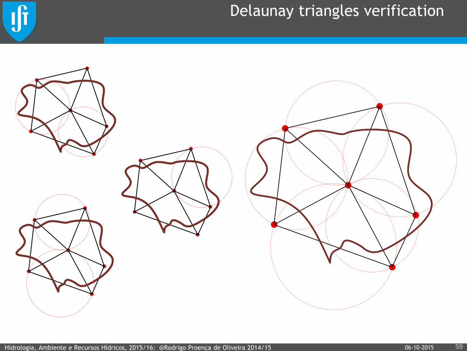
Delaunay triangles verification
Hidrologia, Ambiente e Recursos Hídricos, 2015/16: @Rodrigo Proença de Oliveira 2014/15 59 06-10-2015
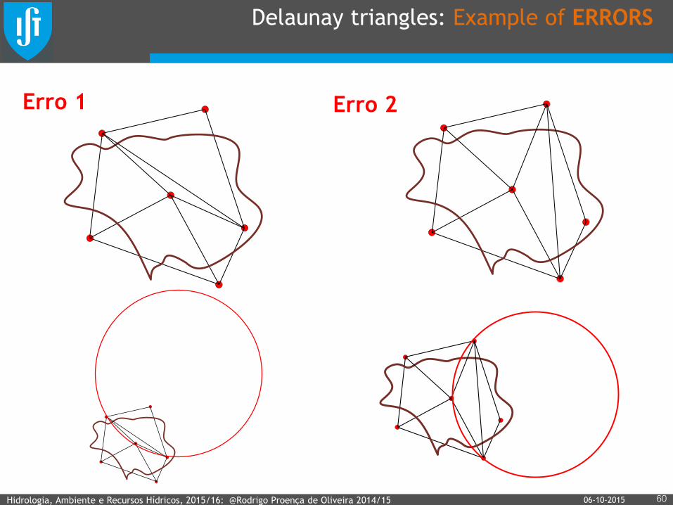
Delaunay triangles: Example of ERRORS
Hidrologia, Ambiente e Recursos Hídricos, 2015/16: @Rodrigo Proença de Oliveira 2014/15 60
Erro 1 Erro 2
06-10-2015
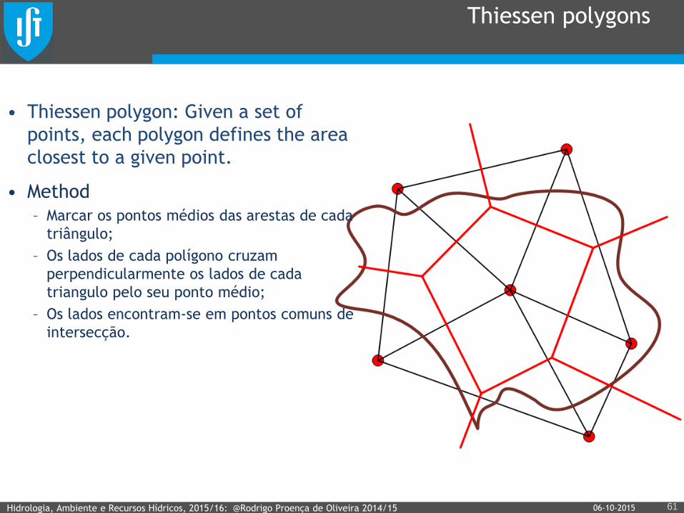
Thiessen polygons
• Thiessen polygon: Given a set of
points, each polygon defines the area
closest to a given point.
• Method
– Marcar os pontos médios das arestas de cada
triângulo;
– Os lados de cada polígono cruzam
perpendicularmente os lados de cada
triangulo pelo seu ponto médio;
– Os lados encontram-se em pontos comuns de
intersecção.
Hidrologia, Ambiente e Recursos Hídricos, 2015/16: @Rodrigo Proença de Oliveira 2014/15 61 06-10-2015
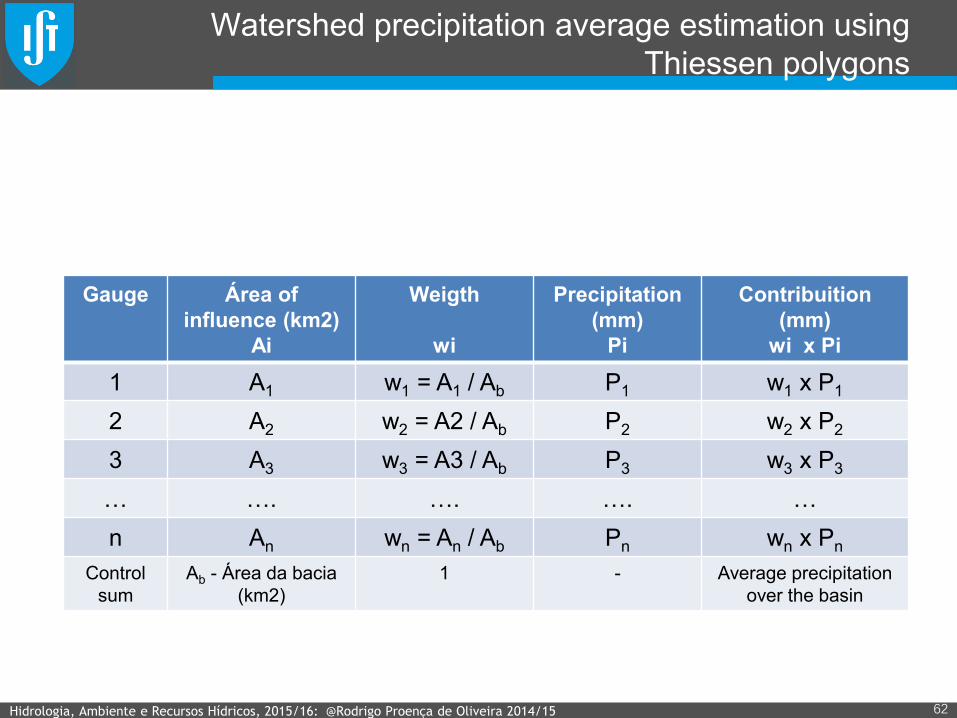
Watershed precipitation average estimation using
Thiessen polygons
Hidrologia, Ambiente e Recursos Hídricos, 2015/16: @Rodrigo Proença de Oliveira 2014/15 62
Gauge Área of
influence (km2)
Ai
Weigth
wi
Precipitation
(mm)
Pi
Contribuition
(mm)
wi x Pi
1 A1 w1 = A1 / Ab P1 w1 x P1
2 A2 w2 = A2 / Ab P2 w2 x P2
3 A3 w3 = A3 / Ab P3 w3 x P3
… …. …. …. …
n An wn = An / Ab Pn wn x Pn
Control
sum
Ab - Área da bacia
(km2)
1 - Average precipitation
over the basin
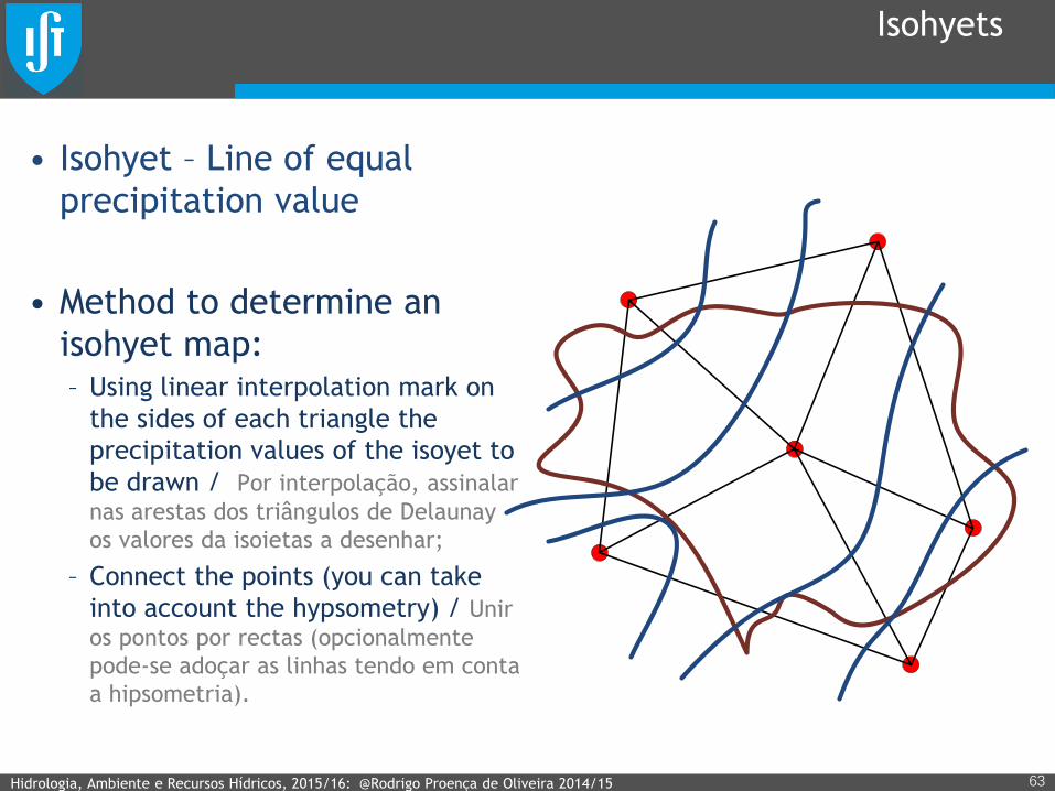
Isohyets
• Isohyet – Line of equal
precipitation value
• Method to determine an
isohyet map: – Using linear interpolation mark on
the sides of each triangle the
precipitation values of the isoyet to
be drawn / Por interpolação, assinalar
nas arestas dos triângulos de Delaunay
os valores da isoietas a desenhar;
– Connect the points (you can take
into account the hypsometry) / Unir
os pontos por rectas (opcionalmente
pode-se adoçar as linhas tendo em conta
a hipsometria).
Hidrologia, Ambiente e Recursos Hídricos, 2015/16: @Rodrigo Proença de Oliveira 2014/15 63
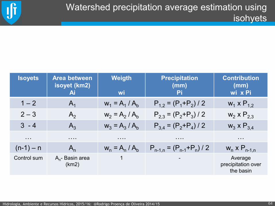
Watershed precipitation average estimation using
isohyets
Hidrologia, Ambiente e Recursos Hídricos, 2015/16: @Rodrigo Proença de Oliveira 2014/15 64
Isoyets Area between
isoyet (km2)
Ai
Weigth
wi
Precipitation
(mm)
Pi
Contribution
(mm)
wi x Pi
1 – 2 A1 w1 = A1 / Ab P1,2 = (P1+P2) / 2 w1 x P1,2
2 – 3 A2 w2 = A2 / Ab P2,3 = (P2+P3) / 2 w2 x P2,3
3 - 4 A3 w3 = A3 / Ab P3,4 = (P2+P4) / 2 w3 x P3,4
… …. …. …. …
(n-1) – n An wn = An / Ab Pn-1,n = (Pn-1+Pn) / 2 wn x Pn-1,n
Control sum An- Basin area
(km2)
1 - Average
precipitation over
the basin
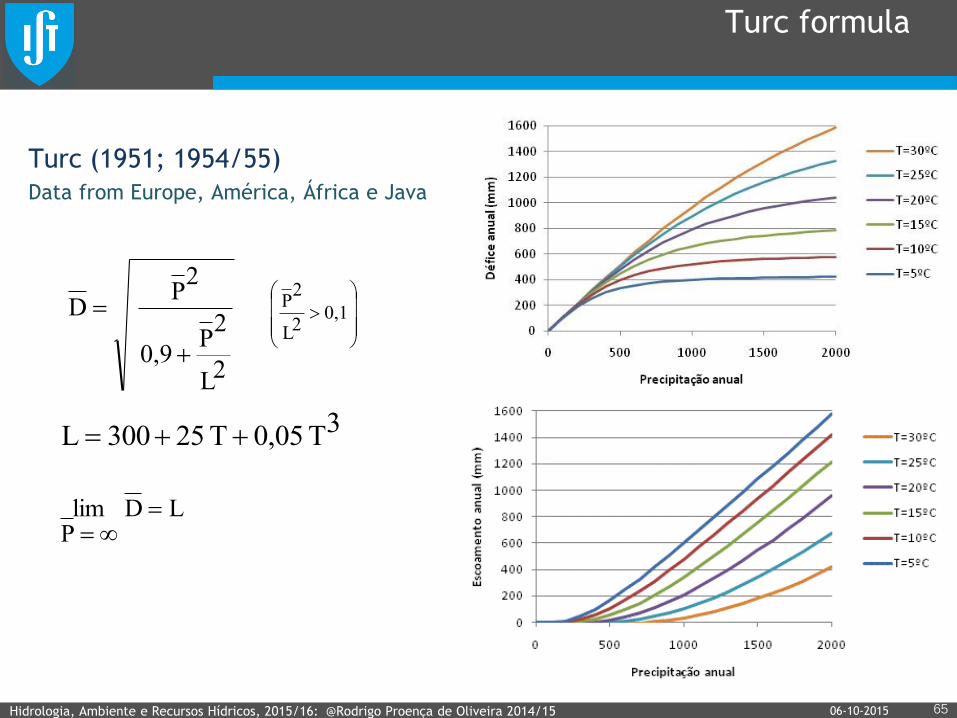
Turc formula
Turc (1951; 1954/55)
Data from Europe, América, África e Java
Hidrologia, Ambiente e Recursos Hídricos, 2015/16: @Rodrigo Proença de Oliveira 2014/15 65
2L
2P
0,9
2P
D
0,1
2L
2P
3T0,05T25300L
LDPlim
06-10-2015
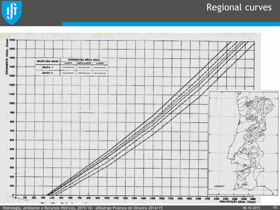
Regional curves
Hidrologia, Ambiente e Recursos Hídricos, 2015/16: @Rodrigo Proença de Oliveira 2014/15 66 06-10-2015