Robotic manipulation of a rotating chainHung Pham Quang-Cuong Pham

Abstract—This paper considers the problem of manipulatinga uniformly rotating chain: the chain is rotated at a constantangular speed around a fixed axis using a robotic manipulator.Manipulation is quasi-static in the sense that transitions are slowenough for the chain to be always in “rotational equilibrium”.The curve traced by the chain in a rotating plane – its shapefunction – can be determined by a simple force analysis, yetit possesses a complex multi-solutions behavior typical of non-linear systems. We prove that the configuration space of theuniformly rotating chain is homeomorphic to a two-dimensionalsurface embedded in R3. Using that representation, we devise amanipulation strategy for transiting between different rotationmodes in a stable and controlled manner. We demonstrate thestrategy on a physical robotic arm manipulating a rotating chain.Finally, we discuss how the ideas developed here might findfruitful applications in the study of other flexible objects, such ascircularly towed aerial systems, elastic rods or concentric tubes.

I. INTRODUCTION

An idle person with a chain in her hand will likely atsome point starts rotating it around a vertical axis, as inFig. 1A. After a while, she might be able to produce anothermode of rotation, whereby the chain would curve inwards,as in Fig. 1B, instead of springing completely outwards.With sufficient dexterity, she might even reach more complexrotation modes, such as in Fig. 1C. Transitions into suchcomplex rotation modes are however difficult to reproducereliably as instabilities can quickly lead to unsustainable rota-tions (Fig. 1D). This paper investigates the mechanics of thetransitions between different rotation modes, and proposes astrategy to perform those transitions in a stable and controlledmanner.

Motivations

There are several reasons why this problem is hard to solve.First, there are multiple solutions for a given control input(distance r between the attached end of the chain and therotation axis, and angular speed ω). This ambiguity makesit difficult to devise a manipulation strategy directly in thecontrol space. Second, some control inputs can quickly leadto “uncontrollable” behaviors of the chain, as illustrated in inFig. 1D.

The theoretical study of the rotating chain and, in particular,of its rotation modes, has a long and rich history in the field ofapplied mathematics [1], [2], [3], [4], [5], [6], [7], which wereview in Section II-A. Here, by devising and implementing

Hung Pham and Quang-Cuong Pham are with Air Traffic ManagementResearch Institute (ATMRI) and Singapore Centre for 3D Printing (SC3DP),School of Mechanical and Aerospace Engineering, Nanyang Technolog-ical University, Singapore. This work was partially supported by grantATMRI:2014-R6-PHAM (awarded by NTU and the Civil Aviation Authorityof Singapore) and by the Medium-Sized Centre funding scheme (awarded bythe National Research Foundation, Prime Minister’s Office, Singapore).

A B C D

Figure 1. Manual rotation of a chain around a vertical axis. A, B, C: Uniformrotation modes 0, 1, 2 respectively. D: Unstable behavior.

a manipulation strategy to stably transit between differentrotation modes, we hope to provide a new, robotics-enabled,understanding of this problem. Indeed, at the core of our ap-proach lie concepts specifically forged in the field of robotics,such as “configuration space”, “stable configurations”, “path-connectivity”, etc.

As opposed to rigid bodies, flexible objects are in generalcharacterized by an infinite number of degrees of freedom,which entails significant challenges when it comes to ma-nipulation. Specific approaches have therefore been developedin the field of robotics to study the manipulation of flexibleobjects, as reviewed in Section II-B.

The above studies are motivated by a number of practicalapplications. For the rotating chain in particular, applicationsinclude aerial manipulation by Unmanned Air Vehicles (UAV),which has recently received some attention, as discussed inmore details in Section II-C.

Contribution and organization of the paper

Our contribution in this paper is threefold. First, we studythe case of arbitrary non-zero attachment radii r (Section IV).This extends and generalizes existing works, which all focuson the case of zero attachment radius, and sets the stagefor stable transitions between different rotation modes, whichspecifically require manipulating the attachment radius. Inparticular, we determine in this section the number of solutionsto the shape equation for any given value r and ω.

Second, we show that the configuration space of theuniformly rotating chain with variable attachment radius ishomeomorphic to a two-dimensional surface embedded in R3

(Section V). We study the subspace of stable configurationsand establish that it is not possible to stably transit betweenrotation modes without going back to the low-amplituderegime.

Third, based on the above results, we propose a manip-ulation strategy for transiting between rotation modes in astable and controlled manner (Section VI). We show the

arX

iv:1

604.

0150

7v2

[cs

.RO

] 5

Sep

201

7

strategy in action in a physical experiment where a roboticarm manipulates a rotating chain and makes it reliably transitbetween different rotation modes.

Before presenting our contribution, we review related works(Section II) and recall Kolodner’s equations of motion ofthe rotating chain (Section III). Finally, we discuss possibleapplications and extensions and sketch some perspectives forfuture work (Section VII).

II. RELATED WORKS

The manipulation of the rotating chain is relevant to anumber of fields such as (i) applied mathematics, (ii) flexibleobject manipulation in robotics, and (iii) aerial manipulation.We now review the literature and describe the position of thecurrent work with respect to each of these fields.

A. Theoretical studies of the rotating chain

In applied mathematics, the study of the rotating chain wasinitiated in 1955 by a remarkable paper by Kolodner [1].Kolodner established the existence of critical speeds (ωi)i∈Nsuch that there are no uniform rotations if the angular speedω < ω1, and there are exactly n rotation modes for ωn < ω <ωn+1. In [2], Caughey studied the rotating chain with small butnon-zero attachment radii. The results obtained by Caugheyextend Kolodner’s and agree with our study of the low-amplitude regime. In [3], Caughey investigated the rotatingchain with both ends attached. In [5], Stuart considered theoriginal rotating chain problem using bifurcation theory, andarrived at the same results as Kolodner. In [4], Wu consideredthe large angular speeds regime. In [7], Toland initiated a newapproach based on the calculus of variation, but did not obtainnew significant results, as compared to Kolodner.

The common point of all previous works is that the chainis attached to the rotation axis, or very close to it [2]. Yet,reliably observing and transiting between different rotationmodes precisely require using arbitrary non-zero attachmentradii r, the distance between the attached end and the rotationaxis. The current paper extends previous studies by specificallyconsidering arbitrary attachment radii.

B. Robotic manipulation of flexible objects

Within the field of robotics, the manipulation of flexibleobjects is studied along two main directions. A first direction istopological: one is mainly interested in the order and sequenceof the manipulation rather than in the precise behavior of theflexible object. Examples include origami folding [8], laundryfolding [9] or rope-knotting [10], [11].

The second research direction is concerned with the preciseshape and dynamics of the manipulated object. Within thisresearch direction, one can distinguish two main approaches.The first approach discretizes the flexible object into a largenumber of small rigid elements, and subsequently carriesout finite-element calculations, see e.g., [12], [6], [13] forinextensible cables or [14], [15] for concentric tube robots.This approach can be applied to any type of flexible objectsas long as a dynamical model is available. However, it usually

yields no qualitative understanding of the manipulation. Forexample, while finite-element calculations can compute theshape of the rotating chain for various control inputs, they canestablish neither the existence of different rotation modes, northe manipulation strategies to transit between different modes.

By contrast, the second approach considers the flexibleobject as the solution of a (partial) differential equation andtries to establish qualitative properties of this solution. Whilethis approach is harder to put in place – usually because ofthe complex mathematical calculations and concepts involved– it can lead to stunning and insightful results. For example,Bretl and colleagues established that the configuration spaceof the Kirchhoff elastic rod is of dimension 6 [16] and thatit is path-connected [17]. Such results would be impossible toobtain via finite-element methods.

The present study of the rotating chain is inscribed withinthis analytical approach. From the dynamic model of therotating chain, we investigate qualitative properties of itsconfiguration space: dimension, connectivity, and stability.These properties are in turn crucial to devise a manipulationstrategy to stably transit between different rotation modes.

C. Aerial manipulation

Although the study of the rotating chain first stemmed out ofscientific curiosity, it has recently found applications in aerialmanipulation. In [13], [18], the authors considered a fixed-wing aircraft towing a long cable whose other end is free.The circular flying pattern imprints a pseudo-stationary shapeto the cable, which in turn allows precisely controlling theposition of the free end. Practical applications of this schemeinclude remote sensing in isolated areas [18], payload deliveryand pickup [12], [19], [18], or more recently, recovery of microair vehicles [20], [21], [22]. In the latter application, the microvehicles are able to attach themselves to the towed end, whichmoves at a relatively slower speed than that of the aircraft.The recent surge of interest in Unmanned Air Vehicles (UAVs)also offers many potential applications: [19] studies a singleUAV flying circularly while towing a cable, [23] deals withgeneral (non-circular) aerial manipulation, while [24] targetscooperative manipulation using a team of UAVs.

The above works are based on dynamic simulation [12],[6], [25], or numerical optimal control [22], [26]. Physicalexperiments were found to agree with simulations [18]. How-ever, there are a number of questions these works are unableto address, for instance: (i) under which conditions are theremultiple solutions to the same set of controls (fly radius andangular speed)? (ii) how to avoid or initiate “jumps” betweendifferent quasi-static rotational solutions [6]? Here, we pre-cisely answer these questions for the case of a simple rotatingchain, without considering aerodynamic drag or end mass.We also discuss how the method can be extended to includethese effects, offering thereby solid theoretical foundationsfor developing safe and stable applications in circular aerialmanipulation.

III. BACKGROUND AND PROBLEM SETTING

A. Equations of motion of the rotating chain

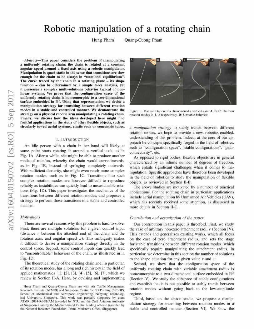
Here we recall the main equations governing the motion ofthe rotating chain initially obtained by Kolodner [1]. Fig. 2depicts an inextensible and homogeneous chain of length Land linear density µ that rotates around a vertical Z-axis. Oneend of the chain is maintained at the attachment radius r fromthe rotation axis, while the other end is free. Note that thecase of a chain with tip mass can be reduced to this case, seeAppendix A.

(x(s,t),y(s,t),z(s,t))

F(L)

s=0

r

ω

φ

x

zy

Rotating plane

ρ(s,t)

s=L

Figure 2. A chain rotating around a fixed vertical axis. At a time instant t,the chain describes a 3D curve parameterized by s: s = 0 at the free end,s = L at the attached end, where L is the length of the chain.

Let x(s, t) := [x(s, t), y(s, t), z(s, t)]> ∈ R3 denote a

length-time parameterization of the chain where s equals zeroat the free end and equals L at the attached end (Fig. 2).Next, let F (s, t) ≥ 0 be the tension of the chain. Neglectingaerodynamic effect, one writes the equation of motion for thechain as

µx = (Fx′)′ + µg, (1)

where � and �′ denote differentiation with respect to t and srespectively; g := [0, 0,−g]> is the gravitational accelerationvector. The inextensibility constraint can be written as

‖x(s, t)′‖2 = 1. (2)

We seek solutions that are uniform rotations; those whichhave constant shape in a plane that rotates around the Z-axis.In this case, the motion of the chain becomes

x(s, t) = ρ(s) cos(ωt),

y(s, t) = ρ(s) sin(ωt),

z(s, t) = z(s),

(3)

where the function ρ(s) is called the shape function of thechain. Directly from inextensibility constraint (2), we have:

‖(ρ(s), z(s))‖2 =√ρ′(s)2 + z′(s)2 = 1. (4)

Also, the tension of the chain F (s, t) is time independent.

Substituting the above expressions into Eq. (1) yields

(Fρ′)′ + µρω2 = 0, (5)(Fz′)′ − µg = 0, (6)

where F, ρ, z are functions of s. Integrating Eq. (6) and notingthat the tension at the free end vanishes (i.e., F (0) = 0) yield

Fz′ =

∫ s

0

µg dλ = µgs. (7)

Next, by the inextensibility constraint (4), we have

F =µgs

z′=

µgs√1− ρ′2

. (8)

Substituting Eq. (8) into Eq. (5) yields the governing equationfor the shape function ρ(s)

d

ds

(µgs√1− ρ′2

ρ′

)+ µρω2 = 0 (9)

subject to the following boundary condition

ρ(L) = r. (10)

Remark that we have applied two boundary conditions: (i)tension at the free end must be zero: F (0, t) = 0 for any t;and (ii) x(L, t) equals the reference trajectory traced by therobotic manipulator (or the aircraft’s trajectory in the towingproblem).

B. Problem formulation

We can now define the configurations and the control inputsof a rotating chain.

Definition 1. (Configuration) A configuration of the rotatingchain is a pair q := (ω, ρ), where ω ≥ 0 is a rotation speedand ρ is a shape function satisfying the governing equation (9)and that ρ(0) ≥ 0. The set of all such configurations is calledthe configuration space of the rotating chain and denoted C.

Definition 2. (Control input) A control input is a pair (r, ω),where r ≥ 0 is an attachment radius and ω ≥ 0 is arotation speed. The set of all inputs is called the control spaceand denoted V . If equation (9) has non-trivial solutions withboundary conditions and parameters defined by the input (r, ω)then the input is called admissible.

Note that the condition ρ(0) ≥ 0 in Definition 1 identifiesduplicate solutions. Any configuration (ω, ρ) corresponds totwo possible solutions: one has shape function ρ and one hasshape function −ρ, both rotate at angular speed ω. The latersolution can be obtained by rotating the former solution by180 degrees. A similar remark applied to the definition of thecontrol space V where we require positive attachment radius.

We can formulate the chain manipulation problem asfollows: given a pair of starting and goal configurations(qinit, qgoal) find a control trajectory (0, 1) → V that bringsthe chain from qinit to qgoal without going through instabilities(instabilities will be discussed in Section V-C).

IV. FORWARD KINEMATICS OF THE ROTATING CHAIN WITHNON-ZERO ATTACHMENT RADIUS

A. Dimensionless shape equation

Still following Kolodner, we convert Eq. (9) into a dimen-sionless equation, more appropriate for subsequent analyses.Consider the changes of variable

u :=ρ′√

1− ρ′2sω2

g, s :=

sω2

g, (11)

which by combining with Eq. (9) leads to

du

ds+ ρ

ω2

g= 0. (12)

One can now differentiate Eq. (12) with respect to s to arriveat

d2

ds2u+ ρ′ = 0,

which is combined with the relation

ρ′ =u√

s2 + u2(13)

to yield the dimensionless differential equation

d2

ds2u(s) +

u(s)√s2 + u(s)

2= 0. (14)

We first consider the boundary condition at s = 0. Bydefinition of u, one has u(0) = 0. The end boundary conditionρ(L) = r implies that

u′(Lω2

g

)= −rω

2

g, (15)

where �′ denotes in this context differentiation with respectto s.

We summarize the boundary conditions on u as

u(0) = 0, u′(L) = r, (16)

whereL := Lω2/g, r := −rω2/g. (17)

This is the standard form of a Boundary Value Problem (BVP).Remark Denote by ρ0 the distance from the free end to theZ-axis. Using Eq. (12), we have

u′(0) = a, (18)

where a = −ρ0ω2/g.

Remark Applying L’Hopital rule twice, one finds that

lims→0

u(s)√s2 + u(s)

2=

a√1 + a2

.

Thus, the differential equation (14) is well-defined at s = 0.

B. Shooting method

We numerically solve the BVP posed in the last sectionusing the simple shooting method [27]. Given a control input(r, ω), the method finds resulting configurations as follows:

1. compute (r, L) from (r, ω) using Eq. (17);

0 5 10 15 20 25 30 35

4

2

0

2

4

6

0 5 10 15 20 25 30 35

5

0

5

10

15

20

25

30

a= a3

a= a2

a= a1

s

u′

u′

(L, 0)

(L, r)A

B

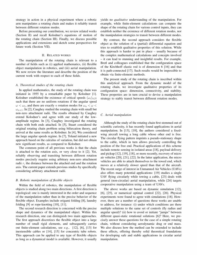
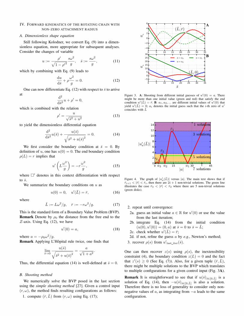
Figure 3. A: Shooting from different initial guesses of u′(0) = a. Theremight be more than one initial value (green and red) that satisfy the endcondition u′(L) = r. B: a1, a2, ... are different initial values of u′(0) thatyield u′(L) = 0; ai denotes the initial guess such that the i-th zero of u′coincides with L

0 15 30 450

2

4

6

8

10

12

14

a3 a2 a1

|u′a(L)|

|a| 7 solutions

5 solutions

3 solutions

1 solution

r3

r2

r1

a3 a2 a1

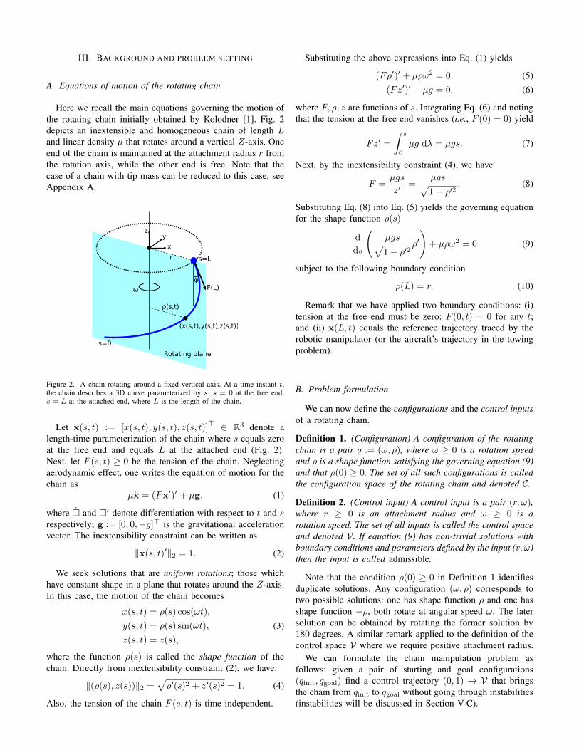
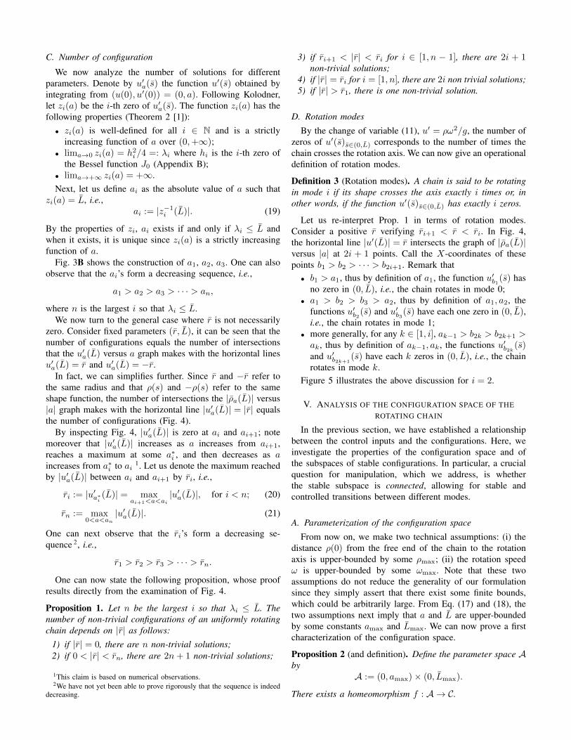
Figure 4. The graph of |u′a(L)| versus |a|. The main text shows that ifri+1 < |r| < ri, then there are 2i+ 1 non-trivial solutions. The green lineillustrates the case r3 < |r| < r2 where there are 5 non-trivial solutions(green disks).

2. repeat until convergence:2a. guess an initial value a ∈ R for u′(0) or use the value

from the last iteration;2b. integrate Eq. (14) from the initial condition

(u(0), u′(0)) = (0, a) at s = 0 to s = L;2c. check whether u′(L) = r;2d. if not, refine the guess a by e.g., Newton’s method;

3. recover ρ(s) from u′last iter(s).

One can then recover z(s) using ρ(s), the inextensibilityconstraint (4), the boundary condition z(L) = 0 and the factthat z′(s) ≥ 0 (See Eq. (7)). Also, for a given tuple (r, L),there might be multiple solutions to the BVP which translatesto multiple configurations for a given control input (Fig. 3A).

Remark It is straightforward to see that if u(s)s∈[0,L] is asolution of Eq. (14), then −u(s)s∈[0,L] is also a solution.Therefore there is no loss of generality to consider only non-negative values of a, as integrating from −a leads to the sameconfiguration.

C. Number of configuration

We now analyze the number of solutions for differentparameters. Denote by u′a(s) the function u′(s) obtained byintegrating from (u(0), u′(0)) = (0, a). Following Kolodner,let zi(a) be the i-th zero of u′a(s). The function zi(a) has thefollowing properties (Theorem 2 [1]):• zi(a) is well-defined for all i ∈ N and is a strictly

increasing function of a over (0,+∞);• lima→0 zi(a) = h2

i /4 =: λi where hi is the i-th zero ofthe Bessel function J0 (Appendix B);

• lima→+∞ zi(a) = +∞.Next, let us define ai as the absolute value of a such that

zi(a) = L, i.e.,ai := |z−1

i (L)|. (19)

By the properties of zi, ai exists if and only if λi ≤ L andwhen it exists, it is unique since zi(a) is a strictly increasingfunction of a.

Fig. 3B shows the construction of a1, a2, a3. One can alsoobserve that the ai’s form a decreasing sequence, i.e.,

a1 > a2 > a3 > · · · > an,

where n is the largest i so that λi ≤ L.We now turn to the general case where r is not necessarily

zero. Consider fixed parameters (r, L), it can be seen that thenumber of configurations equals the number of intersectionsthat the u′a(L) versus a graph makes with the horizontal linesu′a(L) = r and u′a(L) = −r.

In fact, we can simplifies further. Since r and −r refer tothe same radius and that ρ(s) and −ρ(s) refer to the sameshape function, the number of intersections the |ρa(L)| versus|a| graph makes with the horizontal line |u′a(L)| = |r| equalsthe number of configurations (Fig. 4).

By inspecting Fig. 4, |u′a(L)| is zero at ai and ai+1; notemoreover that |u′a(L)| increases as a increases from ai+1,reaches a maximum at some a∗i , and then decreases as aincreases from a∗i to ai 1. Let us denote the maximum reachedby |u′a(L)| between ai and ai+1 by ri, i.e.,

ri := |u′a∗i (L)| = maxai+1<a<ai

|u′a(L)|, for i < n; (20)

rn := max0<a<an

|u′a(L)|. (21)

One can next observe that the ri’s form a decreasing se-quence 2, i.e.,

r1 > r2 > r3 > · · · > rn.

One can now state the following proposition, whose proofresults directly from the examination of Fig. 4.

Proposition 1. Let n be the largest i so that λi ≤ L. Thenumber of non-trivial configurations of an uniformly rotatingchain depends on |r| as follows:

1) if |r| = 0, there are n non-trivial solutions;2) if 0 < |r| < rn, there are 2n+ 1 non-trivial solutions;

1This claim is based on numerical observations.2We have not yet been able to prove rigorously that the sequence is indeed

decreasing.

3) if ri+1 < |r| < ri for i ∈ [1, n − 1], there are 2i + 1non-trivial solutions;

4) if |r| = ri for i = [1, n], there are 2i non trivial solutions;5) if |r| > r1, there is one non-trivial solution.

D. Rotation modes

By the change of variable (11), u′ = ρω2/g, the number ofzeros of u′(s)s∈(0,L) corresponds to the number of times thechain crosses the rotation axis. We can now give an operationaldefinition of rotation modes.

Definition 3 (Rotation modes). A chain is said to be rotatingin mode i if its shape crosses the axis exactly i times or, inother words, if the function u′(s)s∈(0,L) has exactly i zeros.

Let us re-interpret Prop. 1 in terms of rotation modes.Consider a positive r verifying ri+1 < r < ri. In Fig. 4,the horizontal line |u′(L)| = r intersects the graph of |ρa(L)|versus |a| at 2i + 1 points. Call the X-coordinates of thesepoints b1 > b2 > · · · > b2i+1. Remark that• b1 > a1, thus by definition of a1, the function u′b1(s) has

no zero in (0, L), i.e., the chain rotates in mode 0;• a1 > b2 > b3 > a2, thus by definition of a1, a2, the

functions u′b2(s) and u′b3(s) have each one zero in (0, L),i.e., the chain rotates in mode 1;

• more generally, for any k ∈ [1, i], ak−1 > b2k > b2k+1 >ak, thus by definition of ak−1, ak, the functions u′b2k(s)and u′b2k+1

(s) have each k zeros in (0, L), i.e., the chainrotates in mode k.

Figure 5 illustrates the above discussion for i = 2.

V. ANALYSIS OF THE CONFIGURATION SPACE OF THEROTATING CHAIN

In the previous section, we have established a relationshipbetween the control inputs and the configurations. Here, weinvestigate the properties of the configuration space and ofthe subspaces of stable configurations. In particular, a crucialquestion for manipulation, which we address, is whetherthe stable subspace is connected, allowing for stable andcontrolled transitions between different modes.

A. Parameterization of the configuration space

From now on, we make two technical assumptions: (i) thedistance ρ(0) from the free end of the chain to the rotationaxis is upper-bounded by some ρmax; (ii) the rotation speedω is upper-bounded by some ωmax. Note that these twoassumptions do not reduce the generality of our formulationsince they simply assert that there exist some finite bounds,which could be arbitrarily large. From Eq. (17) and (18), thetwo assumptions next imply that a and L are upper-boundedby some constants amax and Lmax. We can now prove a firstcharacterization of the configuration space.

Proposition 2 (and definition). Define the parameter space Aby

A := (0, amax)× (0, Lmax).

There exists a homeomorphism f : A → C.

A

φ

B

φ

C

φ

D

φ

E

φ

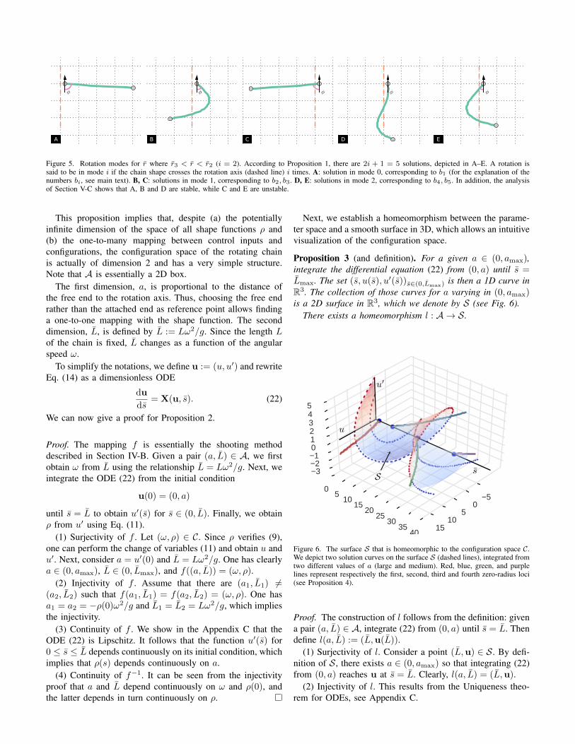
Figure 5. Rotation modes for r where r3 < r < r2 (i = 2). According to Proposition 1, there are 2i + 1 = 5 solutions, depicted in A–E. A rotation issaid to be in mode i if the chain shape crosses the rotation axis (dashed line) i times. A: solution in mode 0, corresponding to b1 (for the explanation of thenumbers bi, see main text). B, C: solutions in mode 1, corresponding to b2, b3. D, E: solutions in mode 2, corresponding to b4, b5. In addition, the analysisof Section V-C shows that A, B and D are stable, while C and E are unstable.

This proposition implies that, despite (a) the potentiallyinfinite dimension of the space of all shape functions ρ and(b) the one-to-many mapping between control inputs andconfigurations, the configuration space of the rotating chainis actually of dimension 2 and has a very simple structure.Note that A is essentially a 2D box.

The first dimension, a, is proportional to the distance ofthe free end to the rotation axis. Thus, choosing the free endrather than the attached end as reference point allows findinga one-to-one mapping with the shape function. The seconddimension, L, is defined by L := Lω2/g. Since the length Lof the chain is fixed, L changes as a function of the angularspeed ω.

To simplify the notations, we define u := (u, u′) and rewriteEq. (14) as a dimensionless ODE

du

ds= X(u, s). (22)

We can now give a proof for Proposition 2.

Proof. The mapping f is essentially the shooting methoddescribed in Section IV-B. Given a pair (a, L) ∈ A, we firstobtain ω from L using the relationship L = Lω2/g. Next, weintegrate the ODE (22) from the initial condition

u(0) = (0, a)

until s = L to obtain u′(s) for s ∈ (0, L). Finally, we obtainρ from u′ using Eq. (11).

(1) Surjectivity of f . Let (ω, ρ) ∈ C. Since ρ verifies (9),one can perform the change of variables (11) and obtain u andu′. Next, consider a = u′(0) and L = Lω2/g. One has clearlya ∈ (0, amax), L ∈ (0, Lmax), and f((a, L)) = (ω, ρ).

(2) Injectivity of f . Assume that there are (a1, L1) 6=(a2, L2) such that f(a1, L1) = f(a2, L2) = (ω, ρ). One hasa1 = a2 = −ρ(0)ω2/g and L1 = L2 = Lω2/g, which impliesthe injectivity.

(3) Continuity of f . We show in the Appendix C that theODE (22) is Lipschitz. It follows that the function u′(s) for0 ≤ s ≤ L depends continuously on its initial condition, whichimplies that ρ(s) depends continuously on a.

(4) Continuity of f−1. It can be seen from the injectivityproof that a and L depend continuously on ω and ρ(0), andthe latter depends in turn continuously on ρ.

Next, we establish a homeomorphism between the parame-ter space and a smooth surface in 3D, which allows an intuitivevisualization of the configuration space.

Proposition 3 (and definition). For a given a ∈ (0, amax),integrate the differential equation (22) from (0, a) until s =Lmax. The set (s, u(s), u′(s))s∈(0,Lmax) is then a 1D curve inR3. The collection of those curves for a varying in (0, amax)is a 2D surface in R3, which we denote by S (see Fig. 6).

There exists a homeomorphism l : A → S.

50

510

15

05

1015

2025

3035

40

321

012345

u′

u

sS

Figure 6. The surface S that is homeomorphic to the configuration space C.We depict two solution curves on the surface S (dashed lines), integrated fromtwo different values of a (large and medium). Red, blue, green, and purplelines represent respectively the first, second, third and fourth zero-radius loci(see Proposition 4).

Proof. The construction of l follows from the definition: givena pair (a, L) ∈ A, integrate (22) from (0, a) until s = L. Thendefine l(a, L) := (L,u(L)).

(1) Surjectivity of l. Consider a point (L,u) ∈ S. By defi-nition of S, there exists a ∈ (0, amax) so that integrating (22)from (0, a) reaches u at s = L. Clearly, l(a, L) = (L,u).

(2) Injectivity of l. This results from the Uniqueness theo-rem for ODEs, see Appendix C.

(3) Continuity of l. From the Continuity theorem for ODEs(Appendix C), it is clear that the end point (L,u(L)) ∈ Sdepends continuously on the initial condition a.

(4) Continuity of l−1. Consider two points(L1,u

∗1), (L2,u

∗2) ∈ S that are sufficiently close to

each other, i.e.,

|L1 − L2| ≤ δ, ‖u∗1 − u∗2‖ ≤ δ,

for some δ that we shall choose later. Consider the curvesu1,u2 such that u1(L1) = u∗1 and u2(L2) = u∗2. By theContinuity theorem (Appendix C) one has for some appropri-ate constant K,

‖u1(0)− u2(0)‖ ≤ eML1‖u1(L1)− u2(L1)‖

≤ eML1(‖u1(L1)− u2(L2))‖+ ‖u2(L2)− u2(L1)‖

)≤ eML1(δ +M |L1 − L2|) = eML1(M + 1)δ,

where the last inequality come from the uniform boundednessof u. For any ε, it suffices therefore to choose δ := εe−ML1

M+1so that |a1 − a2| = ‖u1(0) − u2(0)‖ ≤ ε, which proves thecontinuity of l−1.

Combining Propositions 2 and 3, we obtain the followingtheorem.

Theorem 1. The configuration space C of the rotating chainis homeomorphic to the 2D surface S represented in Fig. 6.

B. Zero-radius loci and low-amplitude regime

Before studying the stable subspaces, we need first to definethe zero-radius loci and the low-amplitude regime in theconfigurations space.

Proposition 4 (and definition). Zero-radius loci are configu-rations whose corresponding attachment radii verify r = 0.Define Li := Lω2

i /g where ωi is the i-th discrete angularspeed (Appendix B). We have the following properties on thesurface S

(i) The i-th zero-radius locus is an infinite curve thatbranches out from the s-axis at (Li, 0, 0), see Fig. 6;

(ii) The i-th zero-radius locus separates configurations inrotation mode i− 1 from those in rotation mode i.

Proof. (i) This property is implied by Kolodner’s results, seethe first paragraph of Sec IV-C for more details.

(ii) Consider a rotation in mode i−1 and the correspondingcurve (s, u1(s), u′1(s))s∈[0,L1]. By definition, u′1(s) has i− 1zeros in the interval [0, L1]. Equivalently, we see that the 3Dcurve (s, u1(s), u′1(s)) crosses the first, second. . . i−1-th zero-radius locus. Now, since the loci start infinitely near the s-axis[point (i)] and extend to infinity, any curve deformed from(s, u1(s), u′1(s))s∈[0,L1] also crosses the same loci.

Consider now another rotation, which is in mode i, and thecorresponding curve (s, u2(s), u′2(s))s∈[0,L2]. By Theorem 1,one can associate the two rotations with their endpoints(L1, u1(L1), u′1(L1)) and (L2, u2(L2), u′2(L2)) on the surfaceS. We will show that any continuous path that connect thesetwo points necessarily crosses the i-th zero-radius locus.

Indeed, assume the contradiction, it follows that there is acontinuous curve ending at (L2, u2(L2), u′2(L2)) that does notcross the i-th locus. This is a contradiction to our assertion inthe first paragraph of point (ii).

We have thus established that the i-th zero-radius locusseparates configurations of rotation mode i − 1 from thosein rotation mode i.

Proposition 5 (and definition). The low-amplitude regimecorresponds to configurations associated with infinitely smallvalues of u(s) and u′(s), for all s ∈ (0, L).

(i) The low-amplitude regime corresponds to points on thesurface S that are infinitely close to the s-axis (in Fig. 6).

(ii) Moreover, this regime corresponds to points on the pa-rameter space A that have small values of a.

Proof. (i) It is clear that a low-amplitude rotation has u(L)and u′(L) infinitely small. Conversely, if u(L) and u′(L) areinfinitely small, by the continuity of the mapping l−1 in theproof of Proposition 3, the initial condition a is also infinitelysmall. Finally, integrating from an infinitely small a will yieldu(s) and u′(s) infinitely small for all s ∈ (0, L).

(ii) This is true from (i).

The low-amplitude rotations with zero attachment radiusthus correspond to (Li, δu, 0), i ∈ N for small values of |δu|.In the sequel, we shall refer to the i-th small-amplitude rotationwith zero radius as the point (Li, 0, 0) instead of the morecorrect phase “(Li, δu, 0) for small values of |δu|”.

C. Stability analysis

So far we have considered the space of all configurationsof the rotating chain, that is, all solutions to the equation ofmotion (1). However, not all configurations are stable; in fact,experiments show that many are not. This section investigatesthe structure of the stable subspace – the subset of stableconfigurations – and discuss stable manipulation strategies.

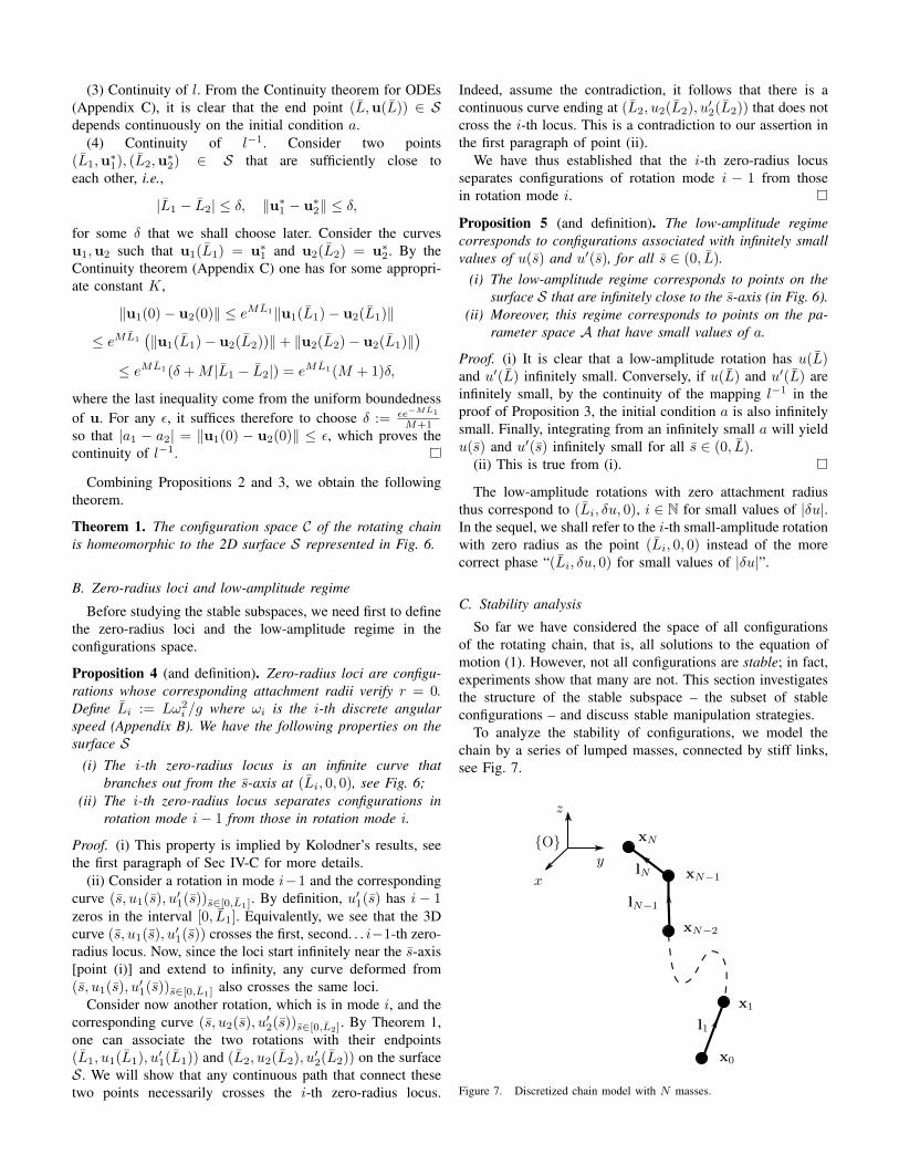
To analyze the stability of configurations, we model thechain by a series of lumped masses, connected by stiff links,see Fig. 7.

x

z

y{O}

x0

x1

xN−2

xN−1

xN

l1

lN−1

lN

Figure 7. Discretized chain model with N masses.

Denote the position of the i-th mass in the rotating frame{O} by xi ∈ R3. The attached end is fixed in {O} at xN .The state of the discretized chain is then given by a 6N -dimensional vector consisting of the positions and velocitiesof the masses

y := [x0, x0, . . . ,xN−1, xN−1]. (23)

Applying Newton’s laws to the masses (see details in Ap-pendix D), one can obtain the dynamics equation

y = f(y). (24)

From Proposition 2, the configurations of the rotating chaincan be represented by a pair (a, L), which is associatedwith the position of the free end x0. Next, we discretize(0, amax) × (0, Lmax) into a 2D grid. For each (a, L) in thegrid, we integrate, from the free end x0, the shape functionof the discretized chain (23) at rotational equilibrium – in thesame spirit as in Proposition 2. This discretized shape functioncorresponds to a state vector yeq := [xeq

0 ,0, . . . ,xeqN−1,0].

Finally, we assess the stability of yeq by looking at theJacobian

J(yeq) :=df

dy(yeq).

Specifically, if the largest real part λmax := maxi Re(λi) ofthe eigenvalues of J(yeq) is positive, then the system is unsta-ble at yeq; if it is negative, then the system is asymptoticallystable at yeq [28, Theorem 3.1].

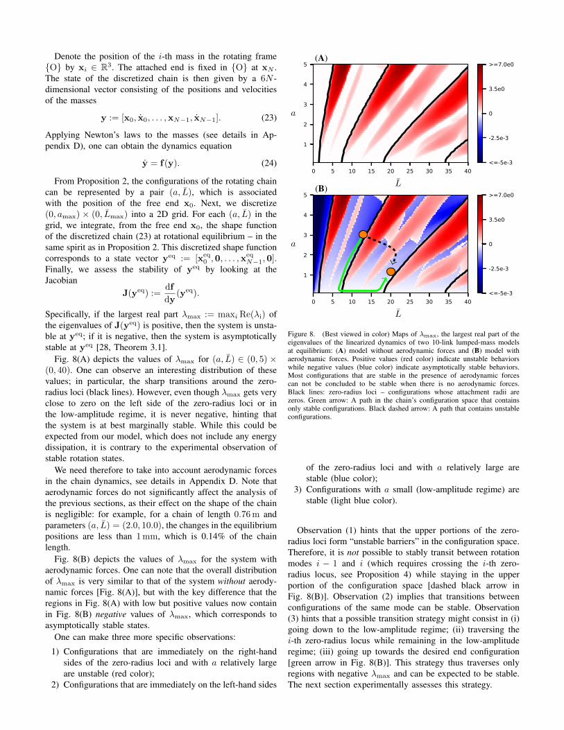
Fig. 8(A) depicts the values of λmax for (a, L) ∈ (0, 5) ×(0, 40). One can observe an interesting distribution of thesevalues; in particular, the sharp transitions around the zero-radius loci (black lines). However, even though λmax gets veryclose to zero on the left side of the zero-radius loci or inthe low-amplitude regime, it is never negative, hinting thatthe system is at best marginally stable. While this could beexpected from our model, which does not include any energydissipation, it is contrary to the experimental observation ofstable rotation states.

We need therefore to take into account aerodynamic forcesin the chain dynamics, see details in Appendix D. Note thataerodynamic forces do not significantly affect the analysis ofthe previous sections, as their effect on the shape of the chainis negligible: for example, for a chain of length 0.76 m andparameters (a, L) = (2.0, 10.0), the changes in the equilibriumpositions are less than 1 mm, which is 0.14% of the chainlength.

Fig. 8(B) depicts the values of λmax for the system withaerodynamic forces. One can note that the overall distributionof λmax is very similar to that of the system without aerody-namic forces [Fig. 8(A)], but with the key difference that theregions in Fig. 8(A) with low but positive values now containin Fig. 8(B) negative values of λmax, which corresponds toasymptotically stable states.

One can make three more specific observations:

1) Configurations that are immediately on the right-handsides of the zero-radius loci and with a relatively largeare unstable (red color);

2) Configurations that are immediately on the left-hand sides

0 5 10 15 20 25 30 35 40

1

2

3

4

5

<=-5e-3

-2.5e-3

0

3.5e0

>=7.0e0

0 5 10 15 20 25 30 35 40

1

2

3

4

5

<=-5e-3

-2.5e-3

0

3.5e0

>=7.0e0(B)

L

a

(A)

L

a

Figure 8. (Best viewed in color) Maps of λmax, the largest real part of theeigenvalues of the linearized dynamics of two 10-link lumped-mass modelsat equilibrium: (A) model without aerodynamic forces and (B) model withaerodynamic forces. Positive values (red color) indicate unstable behaviorswhile negative values (blue color) indicate asymptotically stable behaviors.Most configurations that are stable in the presence of aerodynamic forcescan not be concluded to be stable when there is no aerodynamic forces.Black lines: zero-radius loci – configurations whose attachment radii arezeros. Green arrow: A path in the chain’s configuration space that containsonly stable configurations. Black dashed arrow: A path that contains unstableconfigurations.

of the zero-radius loci and with a relatively large arestable (blue color);

3) Configurations with a small (low-amplitude regime) arestable (light blue color).

Observation (1) hints that the upper portions of the zero-radius loci form “unstable barriers” in the configuration space.Therefore, it is not possible to stably transit between rotationmodes i − 1 and i (which requires crossing the i-th zero-radius locus, see Proposition 4) while staying in the upperportion of the configuration space [dashed black arrow inFig. 8(B)]. Observation (2) implies that transitions betweenconfigurations of the same mode can be stable. Observation(3) hints that a possible transition strategy might consist in (i)going down to the low-amplitude regime; (ii) traversing thei-th zero-radius locus while remaining in the low-amplituderegime; (iii) going up towards the desired end configuration[green arrow in Fig. 8(B)]. This strategy thus traverses onlyregions with negative λmax and can be expected to be stable.The next section experimentally assesses this strategy.

VI. MANIPULATION OF THE ROTATING CHAIN

A. Experiment

We now experimentally test the manipulation strategy enun-ciated in the previous section. More precisely, to stably transitbetween two different rotation modes i and j, we propose to[see the green arrow in Fig. 8(B)]

1) Move from the rotation of mode i towards (Li+1, 0, 0)while staying in the blue region of Fig. 8(B);

2) Move along the L-axis towards (Lj+1, 0, 0);3) Move from (Lj+1, 0, 0) towards the rotation of mode

j while staying in the blue region of blue region ofFig. 8(B).

In practice, the histories of the control inputs (r and ω) toachieve the transitions in steps 1 and 3 can be found by simplelinear interpolation, see e.g. Fig. 9(A).

A

0 50 100 150

Time (s)

0

5

10

15

20

25

An

gu

lar

velo

city

(rads

−1)

A B C D E F 0

5

10

15

20

25A

ttach

me

nt r

ad

ius (m

m)

BA B C D E F

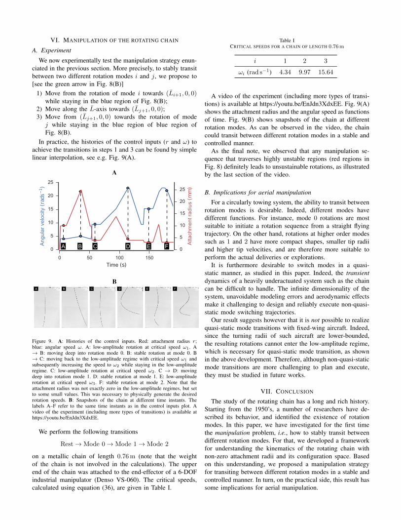
Figure 9. A: Histories of the control inputs. Red: attachment radius r;blue: angular speed ω. A: low-amplitude rotation at critical speed ω1. A→ B: moving deep into rotation mode 0. B: stable rotation at mode 0. B→ C: moving back to the low-amplitude regime with critical speed ω1 andsubsequently increasing the speed to ω2 while staying in the low-amplituderegime. C: low-amplitude rotation at critical speed ω2. C → D: movingdeep into rotation mode 1. D: stable rotation at mode 1. E: low-amplituderotation at critical speed ω3. F: stable rotation at mode 2. Note that theattachment radius was not exactly zero in the low-amplitude regimes, but setto some small values. This was necessary to physically generate the desiredrotation speeds. B: Snapshots of the chain at different time instants. Thelabels A–F refer to the same time instants as in the control inputs plot. Avideo of the experiment (including more types of transitions) is available athttps://youtu.be/EnJdn3XdxEE.

We perform the following transitions

Rest→ Mode 0→ Mode 1→ Mode 2

on a metallic chain of length 0.76 m (note that the weightof the chain is not involved in the calculations). The upperend of the chain was attached to the end-effector of a 6-DOFindustrial manipulator (Denso VS-060). The critical speeds,calculated using equation (36), are given in Table I.

Table ICRITICAL SPEEDS FOR A CHAIN OF LENGTH 0.76 m

i 1 2 3

ωi (rad s−1) 4.34 9.97 15.64

A video of the experiment (including more types of transi-tions) is available at https://youtu.be/EnJdn3XdxEE. Fig. 9(A)shows the attachment radius and the angular speed as functionsof time. Fig. 9(B) shows snapshots of the chain at differentrotation modes. As can be observed in the video, the chaincould transit between different rotation modes in a stable andcontrolled manner.

As the final note, we observed that any manipulation se-quence that traverses highly unstable regions (red regions inFig. 8) definitely leads to unsustainable rotations, as illustratedby the last section of the video.

B. Implications for aerial manipulation

For a circularly towing system, the ability to transit betweenrotation modes is desirable. Indeed, different modes havedifferent functions. For instance, mode 0 rotations are mostsuitable to initiate a rotation sequence from a straight flyingtrajectory. On the other hand, rotations at higher order modessuch as 1 and 2 have more compact shapes, smaller tip radiiand higher tip velocities, and are therefore more suitable toperform the actual deliveries or explorations.

It is furthermore desirable to switch modes in a quasi-static manner, as studied in this paper. Indeed, the transientdynamics of a heavily underactuated system such as the chaincan be difficult to handle. The infinite dimensionality of thesystem, unavoidable modeling errors and aerodynamic effectsmake it challenging to design and reliably execute non-quasi-static mode switching trajectories.

Our result suggests however that it is not possible to realizequasi-static mode transitions with fixed-wing aircraft. Indeed,since the turning radii of such aircraft are lower-bounded,the resulting rotations cannot enter the low-amplitude regime,which is necessary for quasi-static mode transition, as shownin the above development. Therefore, although non-quasi-staticmode transitions are more challenging to plan and execute,they must be studied in future works.

VII. CONCLUSION

The study of the rotating chain has a long and rich history.Starting from the 1950’s, a number of researchers have de-scribed its behavior, and identified the existence of rotationmodes. In this paper, we have investigated for the first timethe manipulation problem, i.e., how to stably transit betweendifferent rotation modes. For that, we developed a frameworkfor understanding the kinematics of the rotating chain withnon-zero attachment radii and its configuration space. Basedon this understanding, we proposed a manipulation strategyfor transiting between different rotation modes in a stable andcontrolled manner. In turn, on the practical side, this result hassome implications for aerial manipulation.

It can be shown (see Appendix A) that all the previousdevelopments can be extended to the case of the chain withnon-negligible tip mass. The key enabling notion here is thatof differential flatness [13], with the flat output being the stateof the free end. By differential flatness, given any trajectory ofthe free end, one can reversely compute the state trajectory andthe control trajectory of the whole system. In fact, the propertythat we have “manually” discovered in this paper – theconfiguration space of a rotating chain is parameterized by theparameter space A – is related to the differential flatness of therotating chain system. Indeed, each point (a, L) corresponds toa circular motion of the free end, which in turn, by differentialflatness, corresponds to the state and control trajectory of thewhole chain, which in turn defines the configuration. Thisobservation suggests two possible extensions:• the motion of the free end can be more general (e.g., an

ellipse), and can thereby lead to more practical applica-tions, such as swinging to hit some position with the tipmass;

• other differentially-flat systems, whose flat output can beparameterized.

Another idea developed here, namely the visualization of theconfiguration space based on forward integration of the shapefunction, might find fruitful applications in the study of otherflexible objects with “mode transition”, such as elastic rods orconcentric tubes subject to “snapping”. Our future work willexplore these possible extensions.

APPENDIX

A. Chain with non-negligible tip mass

Suppose that the free end of the chain carries a drogue ofmass M . We show that all the previous development can beapplied to this more general problem.

We first proceed similarly to Section III and derive thedynamics equation of the rotating chain with tip mass. Writingthe force equilibrium equation at the tip mass yields

F (0)z′(0) = Mg, (25)

F (0)ρ′(0) = −Mρ(0)ω2. (26)

Next, integrate Eq. (25) to obtain

F (s)z(s)′ = g(µs+M), (27)

where µ is again the linear density of the chain. This equationleads to

F (s) = gµs+M√

1− ρ′2. (28)

One arrives at the governing equation

d

ds

(ρ′µs+M√

1− ρ′2

)+ ρ

µω2

g= 0, (29)

with boundary condition ρ(L) = r where r is the attachmentradius. One can now convert Eq. (29) to a dimensionlessequation

d2u

ds2+

u√(s+Mω2/µg)2 + u2

= 0 (30)

by the following changes of variable

u := ρ′µs+M√

1− ρ′2ω2

µg,

s :=sω2

g.

(31)

The boundary conditions are

u′(0) = a, (32)

u(0) = aMω2

µg, (33)

u′(L) = r, (34)

where a = −ρ(0)ω2/g and r = −rω2/g.Eq. (30) is a BVP that can be solved using the shooting

method as described in Section IV-B. Moreover, we see that(a, L) also parameterizes the solution space, which is theconfiguration space of the rotating chain with tip mass.

B. Low-amplitude regime

Here we recall the results obtained by Kolodner [1] for thelow-amplitude regime. Low-amplitude rotations are defined bya zero attachment radius r = 0 and infinitely small values forthe shape function ρ. Linearizing equation (9) about ρ = 0yields

ρw2/g + ρ′ + sρ′′ = 0, (35)

with the boundary condition ρ(L) = 0.By a change of variable v := 2

√sω2/g, one can rewrite

the above equation as

ρv + ρv + ρvvv = 0,

which has solutions of the form

ρ(v) = cJ0(v), i.e.,

ρ(s) = cJ0(2ω√s/g),

where J0 is the zeroth-Bessel function. The boundary condi-tion ρ(L) = 0 then implies that the angular speed can onlytake discrete values (ωi)i∈N where

ωi =hi2

√g/L (36)

where hi is the i-th zero of the Bessel function J0.

C. Useful results from the theory of Ordinary DifferentialEquations

Lemma 1 (Lipschitz). The ordinary differential equation (22)satisfies Lipschitz condition in some convex bounded domainD that contains S.

Proof. Note first that |u′′(u, s)| < 1 for all u, s ∈ R, whichimplies that S is bounded. Set now

D := (0, Lmax)× (uinf , usup)× (u′inf , u′sup),

where uinf , usup, u′inf , u′sup are bounds on S. Clearly, D is

bounded, convex and contains S . Next, all partial derivatives

∂Xi

∂xjare continuous in D (with continuation at s = 0, see

Remark in Section IV-A). This implies that X is Lipschitz inD [29].

We now recall two standard theorems in the theory ofOrdinary Differential Equations, see e.g., [29].

Theorem 2 (Uniqueness). If the vector field X(u, t) satisfiesLipschitz condition in a domain D, then there is at most onesolution u(t) of the differential equation

du

dt= X(u, t)

that satisfies a given initial condition u(a) = c ∈ D.

Theorem 3 (Continuity). Let u1(t) and u2(t) be any twosolutions of the differential equation X(u, t) in T1 ≤ t ≤ T2,where X(u, t) is continuous and Lipschitz in some domain Dthat contains the region where u1(t) and u2(t) are defined.Then, there exists a constant M such that

‖u1(t)− u2(t)‖ ≤ eM |t−a|‖u(a)− y(a)‖

for all a, t ∈ [T1, T2].

D. The discretized chain model

Here we describe the procedure to obtain Eq. (24), whichis the dynamics equation of the discretized chain modelemployed in Section V-C, see also Fig. 7.

The net force Fi acting on the i-th mass is the sum of thefollowing three components:

1) fictitious forces, which include the Coriolis force andcentrifugal force associated with the rotating frame;

2) constraint forces generated by the i-th and i+ 1-th links;3) aerodynamic forces, which include drag and lift.

Fictitious forces are computed using standard formulas, whichcan be found in any textbook on classical mechanics. Tocompute the constraint forces, we model the links as stiff linearsprings whose stiffness approximates that of the chain used inthe experiment of Section VI, which was ' 8× 107 N/m.Constraint forces are then computed using Hooke’s law.

Next, to compute aerodynamic forces, we follow the mod-elling choices of [18], i.e. the aerodynamic forces acting onthe i-th link is placed entirely on the i-th mass. Specifically,define the link length vector as li := xi−xi−1 and denote byvi the actual air speed of the i-th mass, the angle of attack ofthe i-th link is given by

cos ξi = − li · vi‖li‖‖vi‖

.

The drag and lift acting on the i-th link are then given by

FDi = 0.5ρaCD‖li‖d‖vi‖2eD,FLi = 0.5ρaCL‖li‖d‖vi‖2eL,

where the directions and coefficents of drag and lift are

eD = − vi‖vi‖

, eL = − (vi × li)× vi‖(vi × li)× vi‖

,

CD = Cf + Cn sin3(ξi), CL = Cn sin2 ξi cos ξi.

In the above equations, d denotes the diameter of the chain,Cf and Cn are respectively the skin-fraction and crossflowdrag coefficients, ρa is the air density. These parameters havethe following numerical values

d = 1 mm, ρa = 1.225 kg/m3,

Cf = 0.038, Cn = 1.17.

Summing the components we obtain the i-th net force Fi,from which the acceleration of the i-th mass can be found as

xi = Fi/mi,

where mi is the mass of the i-th mass. Rearranging the terms,one obtains the dynamics equation (24)

y = f(y).

REFERENCES

[1] I. I. Kolodner, “Heavy rotating string – a nonlinear eigenvalue problem,”Communications on Pure and Applied Mathematics, vol. 8, no. 3, pp.395–408, aug 1955.

[2] T. K. Caughey, “Whirling of a heavy chain,” in Third U. S. NationalCongress of Applied Mechanics, 1958.

[3] ——, “Large Amplitude Whirling of an Elastic String–a NonlinearEigenvalue Problem,” SIAM Journal on Applied Mathematics, vol. 18,no. 1, pp. 210–237, jan 1970.

[4] C.-H. Wu, “Whirling of a String at Large Angular Speeds—A NonlinearEigenvalue Problem with Moving Boundary Layers,” SIAM Journal onApplied Mathematics, vol. 22, no. 1, pp. 1–13, jan 1972.

[5] C. A. Stuart, “Steadily rotating chains,” in Applications of Methods ofFunctional Analysis to Problems in Mechanics. Springer, 1976, pp.490–499.

[6] J. J. Russell and W. J. Anderson, “Equilibrium and Stability of a Circu-larlyTowed Cable Subject to Aerodynamic Drag,” Journal of Aircraft,vol. 14, no. 7, pp. 680–686, 1977.

[7] J. Toland, “On the stability of rotating heavy chains,” Journal ofDifferential Equations, vol. 32, no. 1, pp. 15–31, apr 1979.

[8] D. J. Balkcom and M. T. Mason, “Robotic origami folding,” TheInternational Journal of Robotics Research, vol. 27, no. 5, pp. 613–627, 2008.

[9] S. Miller, J. Van Den Berg, M. Fritz, T. Darrell, K. Goldberg, andP. Abbeel, “A geometric approach to robotic laundry folding,” TheInternational Journal of Robotics Research, vol. 31, no. 2, pp. 249–267, 2012.

[10] H. Wakamatsu, E. Arai, and S. Hirai, “Knotting/unknotting manipulationof deformable linear objects,” The International Journal of RoboticsResearch, vol. 25, no. 4, pp. 371–395, 2006.

[11] Y. Yamakawa, A. Namiki, and M. Ishikaw, “Dynamic High-speed Knot-ting of a Rope by a Manipulator,” International Journal of AdvancedRobotic Systems, p. 1, 2013.

[12] R. a. Skop and Y. I. Choo, “The configuration of a cable towed in acircular path.” Journal of Aircraft, vol. 8, no. 11, pp. 856–862, 1971.

[13] R. M. Murray, “Trajectory generation for a towed cable system usingdifferential flatness,” in IFAC world congress, 1996, pp. 395–400.

[14] H. B. Gilbert, D. C. Rucker, and R. J. W. Iii, “Concentric Tube Robots:The State of the Art and Future Directions,” International Symposiumon Robotics Research, pp. 1–16, 2013.

[15] D. C. Rucker, B. A. Jones, and R. J. Webster, “A model for concentrictube continuum robots under applied wrenches,” in Proceedings - IEEEInternational Conference on Robotics and Automation, 2010, pp. 1047–1052.

[16] T. Bretl and Z. McCarthy, “Quasi-static manipulation of a kirchhoffelastic rod based on a geometric analysis of equilibrium configurations,”The International Journal of Robotics Research, vol. 33, no. 1, pp. 48–68, 2014.

[17] A. Borum and T. Bretl, “The free configuration space of a kirchhoffelastic rod is path-connected,” in Robotics and Automation (ICRA), 2015IEEE International Conference on. IEEE, 2015, pp. 2958–2964.

[18] P. Williams and P. Trivailo, “Dynamics of Circularly Towed Aerial CableSystems, Part I: Optimal Configurations and Their Stability,” Journal ofGuidance, Control, and Dynamics, vol. 30, no. 3, pp. 753–765, 2007.

[19] M. Merz and T. A. Johansen, “Feasibility study of a circularly towedcable-body system for UAV applications,” in Unmanned Aircraft Systems(ICUAS), 2016 International Conference on. IEEE, 2016, pp. 1182–1191.

[20] M. B. Colton, L. Sun, D. C. Carlson, and R. W. Beard, “Multi-vehicle dynamics and control for aerial recovery of micro air vehicles,”International Journal of Vehicle Autonomous Systems, vol. 9, p. 78,2011.

[21] J. Nichols and L. Sun, “Autonomous Aerial Rendezvous Of SmallUnmanned Aircraft Systems Using A Towed Cable System,” Journalof Guidance, Control, and Dynamics, vol. 37, no. 4, pp. 1–12, 2014.[Online]. Available: http://arc.aiaa.org/doi/abs/10.2514/1.62220

[22] L. Sun, J. D. Hedengren, and R. W. Beard, “Optimal TrajectoryGeneration using Model Predictive Control for Aerially Towed CableSystems,” {AIAA} Journal of Guidance, Control and Dynamics, vol. 37,no. 2, pp. 525–539, 2014.

[23] K. Sreenath, N. Michael, and V. Kumar, “Trajectory generation andcontrol of a quadrotor with a cable-suspended load-a differentially-flat hybrid system,” in Robotics and Automation (ICRA), 2013 IEEEInternational Conference on. IEEE, 2013, pp. 4888–4895.

[24] N. Michael, J. Fink, and V. Kumar, “Cooperative manipulation andtransportation with aerial robots,” Autonomous Robots, vol. 30, no. 1,pp. 73–86, 2011.

[25] P. Williams, D. Sgarioto, and P. M. Trivailo, “Constrained path-planningfor an aerial-towed cable system,” Aerospace Science and Technology,vol. 12, no. 5, pp. 347–354, 2008.

[26] P. Williams and P. Trivailo, “Dynamics of Circularly Towed CableSystems, Part 2: Transitiional Flight and Deployment Control,” AIAAJournal of Guidance, Control, and Dynamics, vol. 30, no. 3, pp. 766–779, 2007.

[27] J. Stoer and R. Bulirsch, “Introduction to Numerical Analysis,” p. 96,1982.

[28] H. K. Khalil, Noninear Systems. Prentice-Hall, New Jersey, 1996.[29] J. Hu and W.-P. Li. (2005) Theory of ordinary differential

equations. [Online]. Available: https://www.math.ust.hk/∼mamu/courses/303/Notes.pdf