Humanitarian Mapping with Deep Learning

Lars RoemheldStanford University

roemheld@stanford.edu

Abstract

This paper uses satellite imagery to support map cre-ation in the developing world. I gather my own dataset bydownloading imagery released through the U.S. State De-partment’s MapGive project and using map data providedby the Humanitarian OpenStreetMap Team. Using thisdata, I train several Convolutional Neural Network modelsdesigned after the SegNet architecture to perform semanticimage segmentation. The output of these models are map-like images that may in a later step be used to reconstructmap data, accelerating the work of online remote mappingvolunteers. This paper details progress made towards thisgoal; my best model’s pixel-average test accuracy of about69% does not allow production use yet. I conclude on notesfor future work.

1. IntroductionWhen natural or other disasters strike, the most endan-

gered people often live in areas that are not well-mapped:in the developing world, whole regions are lacking detailedinformation on where exactly people live, and where criticalinfrastructure is located. Recognizing the need for such datain humanitarian relief missions, the Humanitarian Open-StreetMap Team (HOT)1 has been founded as a team withinthe open-source mapping community OpenStreetMap2: ituses online volunteer workers around the globe to createmissing maps in areas that need it most. Amongst otherachievements, HOT has been recognized for its impact incoordinating relief missions after the 2010 earthquake inHaiti.

The importance of humanitarian mapping efforts hasbeen recognized by the U.S. Department of State in theform of the MapGive initiative3, which makes availableU.S.-licensed satellite imagery for humanitarian mappingefforts. This paper aims to support the volunteer effortswithin HOT and MapGive by using Convolutional Neural

1https://hotosm.org/2http://www.openstreetmap.org/3http://mapgive.state.gov/

Networks (ConvNets) to accelerate the mapping processand reduce necessary volunteer involvement. To this end,I use MapGive imagery and HOT-created maps in my train-ing and testing steps.

A large part of this project has been integrating with ex-isting HOT technology to collect sufficient training data.The following section will detail the process of data collec-tion and describe the collected dataset. Section 3 presentsrelated work and literature, motivating my methods that Ipresent in section 4. Preliminary results are shown in sec-tion 5. Section 6 concludes this paper and discusses futurework.

2. Data

To integrate with existing HOT infrastructure and allowpotential production use of my results, I closely followedthe existing HOT workflows: the team’s current interface isthe “OSM Tasking Manager,” which breaks larger areas intoindividual map-squares that can be assigned to individualvolunteers. For map creation, supporting satellite imageryis overlaid in the project’s map editor, allowing tracing ofroads, buildings, waterways, etc.

Once a task has been worked on, it can be marked as“done”. This lets other volunteers know that the task isready for validation; once another volunteer has marked thetask as “validated,” it is considered finished and removed.For my data collection, I crawled the task manager and sep-arately downloaded the satellite imagery and finished mapdata for “validated” map-squares from MapGive and HOTtile-servers. For easier handling of the data, I also down-loaded raw map data (geojson) through OpenStreetMap’sOverpass API.

Using this data pipeline, it is possible to (a) learn fromfuture volunteer work and (b) feed ConvNet results backinto the existing HOT task manager as “done,” promptinghuman verification before results are released. If a highenough accuracy is achieved, this may significantly speedup the volunteer mapping process.

As my training data, I downloaded two finished HOTprojects in full, spanning roughly 150km2 in Haiti and

1

label % of pixelsnolabel 79.4%building 11.2%road 4.0%farmland 2.6%wetland 1.6%forrest 1.0%river 0.2%

Table 1: Per-pixel distribution of class labels in dataset.

Colombia. At a resolution of 0.6m/pixel,4 this corre-sponds to 10403 individual tiles of 256*256 RGB pixelseach (squares of 153m side length). I preprocessed thesatellite images by subtracting the mean image (i.e. themean color per pixel location), which had the side-effectof partially washing out watermarking (“Digital Globe,” thesatellite image provider). For each of the squares, I thendownloaded the raw map data and a map image accordingto latitude/longitude bounding boxes.

From the map image I generated my final labels by re-placing colors according to a map legend. This added noiseto my image labels, as artifacts such as text-labels, mapicons, anti-aliasing, etc. could not be fully recovered fromthe map image; unfortunately, custom map renderings ofthe OpenStreetMap data were not available in a straight-forward way. This means that labels are noisy, adding toslight label misalignment due to bounding-box inaccuraciesand existing mapping errors. Figure 1 shows a sample ofmy data.

The data suffers from some class imbalance, as shown intable 1: the majority of pixels do not have any label asso-ciated with them. This is due to foresty “bush” areas thatmake up large patches between urban settlements.

I randomly split the dataset into a training set (85%),a validation set (10%) and a test set (5%) and validatedthat the per-pixel label frequencies are roughly equally dis-tributed amongst all sets.

3. Related workXie et al. [15] report remarkable results of their ConvNet

architecture to predict regional poverty levels based offsatellite imagery: using a pre-trained VGG network [13],they first train an image-classification model to predictnight-time light intensities from day-time satellite imagery.In a second step, they transfer the learned features into adirect predictor of poverty levels, achieving almost survey-level results. The authors rely heavily on transfer learn-ing to compensate for label sparsity, and they use a resam-pling method to counteract class imbalance. As their predic-

4This corresponds to TMS/Slippy Map zoom level 18.

tion depends more on macro-level features, they use GoogleMaps5 satellite imagery at a low resolution of 2.4m/pixel,6

– this is 16-times less pixels for the same geographic squarethan used in this paper. In what appears to be a very similarapproach, Facebook researchers have recently reported im-pressive results obtained by significantly larger datasets andnetworks across a wide variety of geographies [7].

Castelluccio et al. [4] present an image classifi-cation model that mainly uses the publicly availableUCMerced dataset [16]. They employ the CaffeNet7

and GoogLeNet [14] architectures, pre-trained on Im-ageNet challenge data [12]. Their strongest result, aversion of GoogLeNet, achieves 97% accuracy on thedataset’s 21 balanced classes, which range from denseresidential to specific (and easily recognized) classessuch as baseball diamond.

Bergman [3] uses the success of image-classificationmodels to produce map images from aerial photos obtainedfrom Google Maps: by classifying the center pixel of animage patch and moving this patch over the input image,the author produces a semantic segmentation which he thenpost-processes.

Mnih and Hinton [11] specifically address the issue ofnoisy labels in map segmentation, which they broadly clas-sify into “omission noise” (missing labels in maps) and“registration noise” (misalignment between map and aerialimage). They propose an Expectation-Maximization (EM)method to iteratively update model beliefs on these formsof noise, and then use these beliefs to augment the segmen-tation loss function. The authors report significant perfor-mance improvements in their ConvNet segmentation.

Within general image segmentation, the SegNet archi-tecture [1] presents a very general, state-of-the-art coresegmentation solution. Originally developed for streetscene segmentation during autonomous driving, the fully-convolutional model appends an “inverted” VGG net-work [13] after a regular VGG network (after removing allnon-convolutional layers) to obtain an encoder and a de-coder phase of the model. In their architecture, the authorspropose an efficient way to maintain spatial information forthe decoder step, which enables a very structured networkthat generates pixel-wise labels (see the following section).In an interesting extension [9], the authors propose a MonteCarlo method to obtain an uncertainty measure of their seg-mentation results, which may be useful during interpreta-tion.

Finally, Basu et al. [2] present a highly specific modelfor satellite imagery, and compare it to various other clas-sification algorithms. They propose a model that uses a

5Due to licensing issues, Google Maps data is unfortunately not avail-able to the Humanitarian OpenStreetMap team.

6This corresponds to TMS/Slippy Map zoom level 16.7CaffeNet is a slightly modified version of AlexNet [10], distributed

with the caffe package [8]

2

(a) Satellite image (b) Map image (c) Segmentation label

Figure 1: Samples from the input dataset: a mean-centered satellite image, the corresponding map image, and the derivedclass labels (colored for easier recognition). Artifacts (noise) created by the text labels and icons are clearly visible. Thesegmentation task is to create a segmentation, given only a satellite image.

deep belief network on 150 statistical and image-processingfeatures generated from satellite imagery to obtain classifi-cation results that are reported to significantly outperformConvNets models on more complex datasets. Analyzing thestatistical properties of their feature space, the authors notethat properties beyond the ConvNet-typical edge-detectionand color-filters are relevant for aerial images.

4. Methods & Models

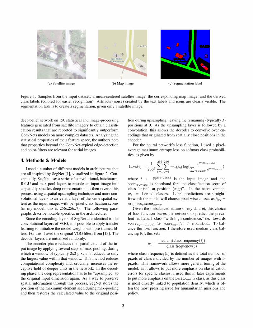
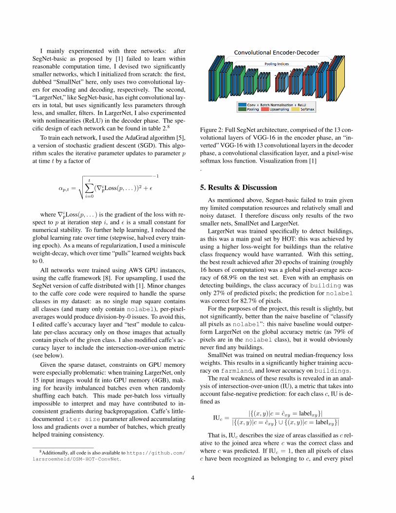
I used a number of different models in architectures thatare all inspired by SegNet [1], visualized in figure 2. Con-ceptually, SegNet uses a series of convolutional, batchnorm,ReLU and max-pool layers to encode an input image intoa spatially smaller, deep representation. It then reverts thisprocess using a spatial upsampling technique and more con-volutional layers to arrive at a layer of the same spatial ex-tent as the input image, with per-pixel classification scores(in my model, this is 256x256x7). The following para-graphs describe notable specifics in the architecture.

Since the encoding layers of SegNet are identical to theconvolutional layers of VGG, it is possible to apply transferlearning to initialize the model weights with pre-trained fil-ters. For this, I used the original VGG filters from [13]. Thedecoder layers are initialized randomly.

The encoder phase reduces the spatial extend of the in-put image by applying several steps of max-pooling, duringwhich a window of typically 2x2 pixels is reduced to onlythe largest value within that window. This method reducescomputational complexity and, crucially, increases the re-ceptive field of deeper units in the network. In the decod-ing phase, the deep representation has to be “upsampled” tothe original input dimension again. As a way to preservespatial information through this process, SegNet stores theposition of the maximum element seen during max-poolingand then restores the calculated value to the original posi-

tion during upsampling, leaving the remaining (typically 3)positions at 0. As the upsampling layer is followed by aconvolution, this allows the decoder to convolve over en-codings that originated from spatially close positions in theencoder.

For the neural network’s loss function, I used a pixel-average maximum entropy loss on softmax class probabili-ties, as given by

Loss(i) =1

2562

256∑x=1

256∑y=1

−wlabel log(escorexy=label∑

c∈classes escorexy=c

)

where i ∈ R256∗256∗3 is the input image and andscorexy=label is shorthand for “the classification score ofclass label at position (x, y)”. In the naive version,wc = 1∀c ∈ classes. Label predictions are straight-forward: the model will choose pixel-wise classes as cxy =argmaxc scorexy=c.

Given the imbalanced nature of my dataset, this choiceof loss function biases the network to predict the preva-lent nolabel class “with high confidence,” i.e. towardsscorexy=nolabel � scorexy=c∀c 6= nolabel. To bal-ance the loss function, I therefore used median class bal-ancing [6]; this sets

wc =mediani(class frequency(i))

class frequency(c)

where class frequency(c) is defined as the total number ofpixels of class c divided by the number of images with c-pixels. This framework allows more general tuning of themodel, as it allows to put more emphasis on classificationerrors for specific classes; I used this in later experimentsto put more emphasis on the building class, as this classis most directly linked to population density, which is of-ten the most pressing issue for humanitarian missions andpolicy.

3

I mainly experimented with three networks: afterSegNet-basic as proposed by [1] failed to learn withinreasonable computation time, I devised two significantlysmaller networks, which I initialized from scratch: the first,dubbed “SmallNet” here, only uses two convolutional lay-ers for encoding and decoding, respectively. The second,“LargerNet,” like SegNet-basic, has eight convolutional lay-ers in total, but uses significantly less parameters throughless, and smaller, filters. In LargerNet, I also experimentedwith nonlinearities (ReLU) in the decoder phase. The spe-cific design of each network can be found in table 2.8

To train each network, I used the AdaGrad algorithm [5],a version of stochastic gradient descent (SGD). This algo-rithm scales the iterative parameter updates to parameter pat time t by a factor of

αp,t =

√√√√ t∑i=0

(∇ipLoss(p, . . . ))2 + ε

−1

where∇ipLoss(p, . . . ) is the gradient of the loss with re-

spect to p at iteration step i, and ε is a small constant fornumerical stability. To further help learning, I reduced theglobal learning rate over time (stepwise, halved every train-ing epoch). As a means of regularization, I used a minisculeweight-decay, which over time “pulls” learned weights backto 0.

All networks were trained using AWS GPU instances,using the caffe framework [8]. For upsampling, I used theSegNet version of caffe distributed with [1]. Minor changesto the caffe core code were required to handle the sparseclasses in my dataset: as no single map square containsall classes (and many only contain nolabel), per-pixel-averages would produce division-by-0 issues. To avoid this,I edited caffe’s accuracy layer and “test” module to calcu-late per-class accuracy only on those images that actuallycontain pixels of the given class. I also modified caffe’s ac-curacy layer to include the intersection-over-union metric(see below).

Given the sparse dataset, constraints on GPU memorywere especially problematic: when training LargerNet, only15 input images would fit into GPU memory (4GB), mak-ing for heavily imbalanced batches even when randomlyshuffling each batch. This made per-batch loss virtuallyimpossible to interpret and may have contributed to in-consistent gradients during backpropagation. Caffe’s little-documented iter size parameter allowed accumulatingloss and gradients over a number of batches, which greatlyhelped training consistency.

8Additionally, all code is also available to https://github.com/larsroemheld/OSM-HOT-ConvNet.

Figure 2: Full SegNet architecture, comprised of the 13 con-volutional layers of VGG-16 in the encoder phase, an “in-verted” VGG-16 with 13 convolutional layers in the decoderphase, a convolutional classification layer, and a pixel-wisesoftmax loss function. Visualization from [1].

5. Results & DiscussionAs mentioned above, Segnet-basic failed to train given

my limited computation resources and relatively small andnoisy dataset. I therefore discuss only results of the twosmaller nets, SmallNet and LargerNet.

LargerNet was trained specifically to detect buildings,as this was a main goal set by HOT: this was achieved byusing a higher loss-weight for buildings than the relativeclass frequency would have warranted. With this setting,the best result achieved after 20 epochs of training (roughly16 hours of computation) was a global pixel-average accu-racy of 68.9% on the test set. Even with an emphasis ondetecting buildings, the class accuracy of building wasonly 27% of predicted pixels; the prediction for nolabelwas correct for 82.7% of pixels.

For the purposes of the project, this result is slightly, butnot significantly, better than the naive baseline of “classifyall pixels as nolabel”: this naive baseline would outper-form LargerNet on the global accuracy metric (as 79% ofpixels are in the nolabel class), but it would obviouslynever find any buildings.

SmallNet was trained on neutral median-frequency lossweights. This results in a significantly higher training accu-racy on farmland, and lower accuracy on buildings.

The real weakness of these results is revealed in an anal-ysis of intersection-over-union (IU), a metric that takes intoaccount false-negative prediction: for each class c, IU is de-fined as

IUc =|{(x, y)|c = cxy = labelxy}|

|{(x, y)|c = cxy} ∪ {(x, y)|c = labelxy}|

That is, IUc describes the size of areas classified as c rel-ative to the joined area where c was the correct class andwhere c was predicted. If IUc = 1, then all pixels of classc have been recognized as belonging to c, and every pixel

4

SegNet-basic SmallNet LargerNetconv7 64 conv3 64BN BNReLU ReLUMaxPool2 MaxPool4

conv7 128 conv 3 64BN ReLUReLUMaxPool2

conv7 256 conv7 64 conv3 128BN BN BNReLU ReLU ReLUMaxPool2 MaxPool4 MaxPool2

conv7 512 conv7 128 conv3 256BN BN ReLUReLU ReLU MaxPool2MaxPool2 MaxPool4

(encoded) (encoded) (encoded)

upsample2 upsample4 upsample2conv7 256 conv7 64 conv3 128BN BN ReLU

upsample2 upsample4 upsample2conv7 128 conv7 64 conv3 128BN BN ReLU

upsample2 conv3 7 conv3 64conv7 64 BNBN ReLU

upsample2 upsample4conv7 64 conv3 64BN BN

ReLU

conv1 7 conv1 7

Table 2: Detailed architecture of the 3 main networks usedin this paper. convX Y denotes a convolutional layer withY filters of size X*X. MaxPoolX denotes a max-poolinglayer with stride X and size X*X. upsampleX denotes up-sampling with size X*X as described here. ReLU denotes arectified linear unit, point-wise y = max(0, x). BN denotesBatch Normalization with learnable shift and scale parame-ters.

classified as c was really a c. For all classes except thedominant nolabel, this metric is almost 0, indicating thatwhile LargerNet does have some accuracy in its predictionof buildings, it misses many areas where it should have de-tected buildings (on the test set, IUnolabel = 62.6% andIUriver = 2.6% are the two highest IU values.)

Table 3 summarizes the most relevant model accuracies.In the remainder of this section, I will provide some quali-tative analysis of the bad model performance.

As is evident by comparing training and test accuracies,the networks did not overfit at all. Given the very low reg-ularization rates, this is likely due to significant noise in thetraining data: the data obtained through MapGive and OSMincludes clouds, glare, and significant false-negatives in the

LargerNet SmallNettraining test training test

average 68.8% 68.9% 60.6% 61%nolabel 83.0% 82.7% 72.2% 72.5%building 25.2% 27.0% 11.6% 13.6%farmland 2.5% 2.5% 23.9% 19.9%river 24.8% 23.9% 28.5% 26.8%

Table 3: Per-pixel average and class average accuracies ofSmallNet and LargerNet. Validation accuracies have beenommitted, as they are almost identical to training and testaccuracies.

map labels.Given “real world data,” noise was to be expected –

more computation time (more epochs) and more trainingdata may have helped overcome some data problems. An-other, more subtle, problem is that with the more shallownets I used (as opposed to a full 26-layer SegNet), evenLargeNet did not have a particularly expressive receptivefield, as much of it was created through big max-poolinglayers. This may help explain why LargeNet is missinglarger structures in images. Figure 3 gives a visual overviewof model performance.

6. ConclusionThe task attempted in this project was ambitious: satel-

lite data is known to be a challenging image recognitiontask [4], and even more so on a segmentation problem with-out a pre-trained model. Through the data pipeline createdfor this project, a large amount of additional training datais available – I was lacking computational power to usesignificantly more data, but recent work on massive aerialimagery datasets seems promising [7]. If successful, thisproject would ultimately help HOT and may offer relief tosome of the world’s most disadvantaged people. I hope tocontinue the project; maybe others will follow my data.

Until now, significant work went into establishing theproject outline and the data pipeline; unfortunately, I did notachieve actionable results yet. Besides more in-depth classbalancing, for example through a re-sampling techniqueduring training, it would be interesting for future work tosee how expectation-maximization models may help modellabel noise and facilitate learning. It may also be interestingto explore feature generation through more sophisticatedimage preprocessing, and to explore different ConvNet ar-chitectures for aerial imagery in a more structured way.

References[1] V. Badrinarayanan, A. Kendall, and R. Cipolla. Segnet: A

deep convolutional encoder-decoder architecture for image

5

(a) Satellite image. Note the hut towards thetop-center.

(b) Ground-truth map image. The hut is miss-ing from the map.

(c) Segmentation result. Noisy, but picked upon the missing building.

(d) Satellite image of residential area. (e) Ground-truth map image.(f) Segmentation picked up some buildings,but failed to get overall structure.

(g) Satellite image of bushland. (h) Ground truth: nothing to see here.(i) Segmentation misinterprets evenly spacedstructure.

Figure 3: Segmentation examples from LargerNet. The first row shows an example of noisy labels, penalizing the networkfor a correct prediction of building. The second row shows an example where the network is missing overall structure.The last row shows an example of false-positives caused by higher weighting of building in the network.

segmentation. CoRR, abs/1511.00561, 2015.

[2] S. Basu, S. Ganguly, S. Mukhopadhyay, R. DiBiano,M. Karki, and R. R. Nemani. Deepsat - A learning frame-work for satellite imagery. CoRR, abs/1509.03602, 2015.

[3] I. Bergman. Extracting map features from satellite images.CS231n Winter Final Report, 2015.

[4] M. Castelluccio, G. Poggi, C. Sansone, and L. Verdoliva.Land use classification in remote sensing images by convo-lutional neural networks. CoRR, abs/1508.00092, 2015.

[5] J. C. Duchi, E. Hazan, and Y. Singer. Adaptive subgra-dient methods for online learning and stochastic optimiza-tion. Journal of Machine Learning Research, 12:2121–2159,2011.

[6] D. Eigen and R. Fergus. Predicting depth, surface normalsand semantic labels with a common multi-scale convolu-tional architecture. CoRR, abs/1411.4734, 2014.

[7] A. Gros and T. Tiecke. Connecting the world with bettermaps. facebook researcb, 2016.

[8] Y. Jia, E. Shelhamer, J. Donahue, S. Karayev, J. Long, R. Gir-

6

shick, S. Guadarrama, and T. Darrell. Caffe: Convolu-tional architecture for fast feature embedding. arXiv preprintarXiv:1408.5093, 2014.

[9] A. Kendall, V. Badrinarayanan, and R. Cipolla. Bayesiansegnet: Model uncertainty in deep convolutional encoder-decoder architectures for scene understanding. CoRR,abs/1511.02680, 2015.

[10] A. Krizhevsky, I. Sutskever, and G. E. Hinton. Imagenetclassification with deep convolutional neural networks. InF. Pereira, C. J. C. Burges, L. Bottou, and K. Q. Weinberger,editors, Advances in Neural Information Processing Systems25, pages 1097–1105. Curran Associates, Inc., 2012.

[11] V. Mnih and G. Hinton. Learning to label aerial images fromnoisy data. In Proceedings of the 29th Annual InternationalConference on Machine Learning (ICML 2012), June 2012.

[12] O. Russakovsky, J. Deng, H. Su, J. Krause, S. Satheesh,S. Ma, Z. Huang, A. Karpathy, A. Khosla, M. Bernstein,A. C. Berg, and L. Fei-Fei. ImageNet Large Scale VisualRecognition Challenge. International Journal of ComputerVision (IJCV), 115(3):211–252, 2015.

[13] K. Simonyan and A. Zisserman. Very deep convolutionalnetworks for large-scale image recognition. ACM SIGSPA-TIAL International Conference on Advances in GeographicInformation Systems (ACM GIS), 2010.

[14] C. Szegedy, W. Liu, Y. Jia, P. Sermanet, S. Reed,D. Anguelov, D. Erhan, V. Vanhoucke, and A. Rabinovich.Going deeper with convolutions. CoRR, abs/1409.4842,2014.

[15] M. Xie, N. Jean, M. Burke, D. Lobell, and S. Ermon.Transfer learning from deep features for remote sensing andpoverty mapping. CoRR, abs/1510.00098, 2015.

[16] Y. Yang and S. Newsam. Bag-of-visual-words and spatialextensions for land-use classification. CoRR, abs/1409.1556,2014.

7