Embed Size (px)
Citation preview

Background Study Design Empirical Analysis Major Choice
Human Capital Investments and Expectationsabout Career and Family
Matthew Wiswall - ASU; UW MadisonBasit Zafar - NY Fed
The views expressed in this paper reflect those of the authors, and not necessarily those of the New York
Fed or the Federal Reserve System.

Background Study Design Empirical Analysis Major Choice
Introduction
• Traditional view of human capital investments privilege monetarymotivations (“career concerns")
• However, many other factors may be important, such asimplications of human capital choices for future family life (marriageand fertility) and, of course, the pure enjoyment of working inparticular fields or jobs
• Previous work has studied the trade-offs between career and familyby examining the characteristics of already chosen education andjobs, e.g. women more likely than men to choose careers allowinggreater hours flexibility
• We study how individuals perceive the trade-off between career andfamily when they are young and are in the process of making keyhuman capital decisions

Background Study Design Empirical Analysis Major Choice
Background
• Beliefs about the future, not realized outcomes, are crucial tounderstanding decision making
• Given that human capital choices are made when individualsare young and without full information, we would expectconsiderable heterogeneity in beliefs which may not necessarilybe consistent with rational expectations
• Previous work has found considerable heterogeneity in beliefsabout future earnings (Manski, 2004; Jensen, 2009;Arcidiancono et al., 2012; Wiswall and Zafar, 2015)

Background Study Design Empirical Analysis Major Choice
This Paper• Our contribution is to elicit ex ante beliefs for a large set ofevents, conditional on different human capital levels.
• events include expected earnings at multiple ages, marriageprospects, fertility, spousal earnings, labor supply
• human capital levels are college majors (science/business,humanities) and no college
• Analysis of conditional beliefs can reveal how individualsbelieve human capital investments affect a variety of later lifeoutcomes (ex ante treatment effects)
• For example, how marriage likelihood is affected if one were tocomplete a college degree versus not completing a degree
• We investigate whether ex ante beliefs are predictive of futureoutcomes.
• We show that ex ante beliefs about non-wage outcomes arean important determinant of educational choices.

Background Study Design Empirical Analysis Major Choice
Human Capital Investment and BeliefsExpected utility from human capital level k is:
EiVi ,k =T
∑t=1
βt−1∫u(X )dGi (X |k, t),
Gi (X |k, t) is i’s beliefs about the distribution of future events X inperiod t, if the individual were to complete human capitalinvestment k.
• Gi (X |k, t) reflects individual uncertainty about futureoutcomes (e.g. expected probability of working full-time).This is "unresolvable" uncertainty.
• By eliciting Gi (X |k, t) for different levels of human capital,one can estimate the individual-level ex ante treatment effect:Gi (X |k, t)− Gi (X |k ′, t).• Example: Ei (W |k = college, 30)− Ei (W |k ′ = no college, 30)

Background Study Design Empirical Analysis Major Choice
Potential Outcomes
• Fi (X |k, t) is the actual distribution of events which would occur if ichooses human capital level k .
• Rational expectations imposes that Gi (X |k, t) = Fi (X |k, t),element by element.
• We can relax this assumption by directly eliciting beliefs Gi ; theseneed not be equal to the actual realized outcome distribution.
• A common object of interest is the ex post difference in potentialoutcomes
∆F ,i (k, k ′) = Fi (X |k, t)− Fi (X |k ′, t)
Only one choice can be made and only one of the outcomedistributions is realized and observed in standard data.
• A large literature studies how to identify these potential outcomes(e.g. average treatment effects) from realized choice data (e.g.Heckman and Vytlacil, 2005; Angrist and Pischke, 2009; Imbensand Rubin, 2015).

Background Study Design Empirical Analysis Major Choice
Realized Outcomes• The distribution of realized events X for the population whichchooses k, Mk , is
H(X |k, t) = M−1k ∑i∈Ωk
Fi (X |k = k∗, t),
• For a given individual, only one of the outcome distributions isrealized and observed in data.
• The difference in the distribution of outcomes X observed inthe population which chooses human capital k rather k ′ is:
∆H (k , k ′) = H(X |k, t)−H(X |k ′, t)
Note that ∆H (k, k ′) is not indexed by i because it representsa population distribution.
• Identification of choice models using ex post observed data isonly possible by making assumptions on the selection process,and on ex ante beliefs.

Background Study Design Empirical Analysis Major Choice
Related Literature• Human capital investments and returns in the marriage market
• Iyigun and Walsh (2007); Chiappori, Iyigun, and Weiss (2009);Chiappori, Salanie, and Weiss (2015)
• Empirical work generally infers (ex post) returns indirectly: Ge(2011); Lafortune (2013); Attansaio and Kaufmann (2011);Kaufmann et al. (2015)
• Subjective expectations and decision-making under uncertainty• Manski, 2004, has an earlier survey of this literature.Arcidiacono et al. (2012, 2015), Stinebrickner andStinebrickner (2012, 2014), Zafar (2013), Giustinelli (2015),Kaufmann (2015), and Wiswall and Zafar (2015, 2016)
• Educational/Occupational choices and the gender gap• Turner and Bowen (1999); Arcidiacono (2004); Bertrand et al.(2010); Goldin and Katz (2011); Goldin (1997, 2014); Flabbiand Moro (2012); Gemici and Wiswall (2014); Klevin et al.(2015); Wasserman (2015); Bronson (2015)

Background Study Design Empirical Analysis Major Choice
Study Design
• 501 undergraduates at NYU; 317 of them females
• Study conducted during May-June 2010• A 90-minute online survey (constructed using SurveyMonkey)• Compensation: $30 for completing the survey• Survey was part of larger experiment in which we providedstudents with different types of information (Wiswall andZafar, 2014a, b)
• Conduct at follow-up survey in early 2016

Background Study Design Empirical Analysis Major Choice
Survey InstrumentCollect information on life activities that would be plausibledeterminants of college majors
• Each question was conditioned on the choice of 1 of 5potential "majors": (1) Business; (2) Engineering; (3)Humanities; (4) Natural Sciences; (5) Not Graduate.• The analysis aggregates the data to 3 groups:Sciences/Business; Humanities; No College
• Questions for the future were conditioned on three ages: age22; age 30; age 45
• Students asked about future earnings, marriage probability,number of children, spouse’s earnings and labor supply, andself labor supply conditional on marital state
• Collect data on the probability a student believed she wouldgraduate with a major in each field and the subjectivemajor-specific ability ranking of the student
Background Study Design Empirical Analysis Major Choice
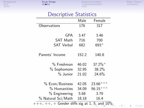
Descriptive StatisticsMale Female
Observations 176 317
GPA 3.47 3.46SAT Math 716 700SAT Verbal 682 693+
Parents’Income 152.2 140.8
% Freshman 46.02 37.2%+
% Sophomore 32.95 38.2%% Junior 21.02 24.6%
% Econ/Business 42.05 23.66+++
% Humanities 34.09 56.15+++
% Engineering 5.68 3.79% Natural Sci/Math 18.18 16.4
+++, ++, + Gender diffs sig at 1, 5, and 10%.

Background Study Design Empirical Analysis Major Choice
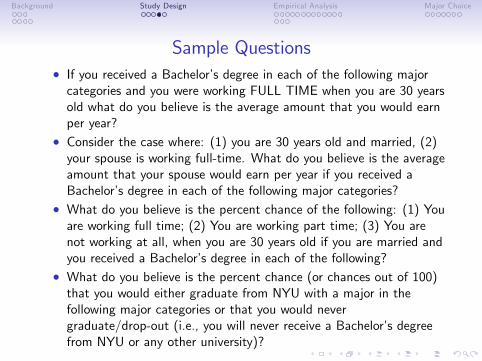
Sample Questions• If you received a Bachelor’s degree in each of the following majorcategories and you were working FULL TIME when you are 30 yearsold what do you believe is the average amount that you would earnper year?
• Consider the case where: (1) you are 30 years old and married, (2)your spouse is working full-time. What do you believe is the averageamount that your spouse would earn per year if you received aBachelor’s degree in each of the following major categories?
• What do you believe is the percent chance of the following: (1) Youare working full time; (2) You are working part time; (3) You arenot working at all, when you are 30 years old if you are married andyou received a Bachelor’s degree in each of the following?
• What do you believe is the percent chance (or chances out of 100)that you would either graduate from NYU with a major in thefollowing major categories or that you would nevergraduate/drop-out (i.e., you will never receive a Bachelor’s degreefrom NYU or any other university)?

Background Study Design Empirical Analysis Major Choice
Sample Questions• If you received a Bachelor’s degree in each of the following majorcategories and you were working FULL TIME when you are 30 yearsold what do you believe is the average amount that you would earnper year?
• Consider the case where: (1) you are 30 years old and married, (2)your spouse is working full-time. What do you believe is the averageamount that your spouse would earn per year if you received aBachelor’s degree in each of the following major categories?
• What do you believe is the percent chance of the following: (1) Youare working full time; (2) You are working part time; (3) You arenot working at all, when you are 30 years old if you are married andyou received a Bachelor’s degree in each of the following?
• What do you believe is the percent chance (or chances out of 100)that you would either graduate from NYU with a major in thefollowing major categories or that you would nevergraduate/drop-out (i.e., you will never receive a Bachelor’s degreefrom NYU or any other university)?

Background Study Design Empirical Analysis Major Choice
ACS 2009 Data (ex post outcomes)
Age 23 Age 30 Age 45Male Female Male Female Male Female
Earnings (in $10,000s)Science/Business 3.3 3.2 6.7 5.5+++ 11.6 7.5+++
Humanities 2.5 2.6 5.4 4.5+++ 9.1 5.9+++
Some College 2.5 2.2+++ 4.2 3.1+++ 5.7 3.9+++
p-value 0 0 0 0 0 0
Spousal Earnings (in $10,000s)Science/Business 3.4 4.8+++ 5.3 8.3+++ 7.4 12.7+++
Humanities 2.3 3.5+++ 4.3 6.7+++ 5.7 9.9+++
Some College 2.2 3.5+++ 3.2 4.8+++ 3.8 6.4+++
p-value 0 0.003 0 0 0 0
Married (%)Science/Business 8.2 15.9+++ 61.7 67.5+++ 80.8 76.1+++
Humanities 11.5 15.3+++ 55.7 64.9+++ 76.6 74.5+
Some College 15.2 26.4+++ 54.9 59.3+++ 69.3 69.6p-value 0 0 0 0 0 0
+++, ++, + gender diffs sig at the 1, 5, and 10% levels.

Background Study Design Empirical Analysis Major Choice
Beliefs about Earnings (in 000s Dollars)
Age 22 Age 30 Age 45Male Female Male Female Male Female
Science/Business 5.9 5.4 13.7 10.9++ 19.0 13.8+++(7.3) (4.7) (16.6) (9.3) (22.4) (14.1)
Humanities 4.7 3.9 6.9 6.9 11.0 9.6(7.4) (3.5) (5.5) (7.4) (13.5) (11.8)
Not Graduate 3.5 2.5++ 5.1 3.3++ 9.0 5.9+++(7.5) (1.2) (11.0) (4.6) (16.0) (10.2)
Overall 5.6 4.7+ 13.0 9.2+++ 18.4 12.3+++(7.4) (3.8) (16.4) (8.5) (22.5) (13.9)
Standard deviations in parentheses.+++, ++, + gender diffs sig at the 1, 5, and 10% levels.

Background Study Design Empirical Analysis Major Choice
Beliefs about Earnings Growth

Background Study Design Empirical Analysis Major Choice
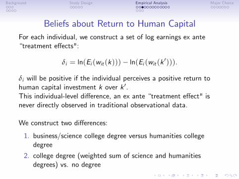
Beliefs about Return to Human CapitalFor each individual, we construct a set of log earnings ex ante“treatment effects":
δi = ln(Ei (wit (k)))− ln(Ei (wit (k ′))).
δi will be positive if the individual perceives a positive return tohuman capital investment k over k ′.This individual-level difference, an ex ante “treatment effect" isnever directly observed in traditional observational data.
We construct two differences:
1. business/science college degree versus humanities collegedegree
2. college degree (weighted sum of science and humanitiesdegrees) vs. no degree
Background Study Design Empirical Analysis Major Choice
Beliefs about Return to Human CapitalFor each individual, we construct a set of log earnings ex ante“treatment effects":
δi = ln(Ei (wit (k)))− ln(Ei (wit (k ′))).
δi will be positive if the individual perceives a positive return tohuman capital investment k over k ′.This individual-level difference, an ex ante “treatment effect" isnever directly observed in traditional observational data.
We construct two differences:
1. business/science college degree versus humanities collegedegree
2. college degree (weighted sum of science and humanitiesdegrees) vs. no degree

Background Study Design Empirical Analysis Major Choice
Beliefs about Returns to Human Capital
Age 22 Age 30 Age 45Male Female Male Female Male Female
Avg Level (000s $) 5.60 4.68+ 12.95 9.21+++ 18.44 12.33+++
Log DiffScience vs. Hum .27 .31 .52 .43++ .45 .35+
(.02) (.02) (.05) (.03) (.05) (.03)Grad vs. Not Grad .59 .64 1.02 1.04 .83 .83
(.03) (.03) (.06) (.04) (.05) (.04)All log diff estimates are significant at the 1% level.+++,++,+ denote gender diff sig. at the 1, 5, and 10% levels.
Earnings at age 30:103% higher with a college degree versus not43-52% higher with a science degree (vs. humanities)

Background Study Design Empirical Analysis Major Choice
Heterogeneity in Ex ante Returns

Background Study Design Empirical Analysis Major Choice
Beliefs about Earnings GrowthAge 23-30 Age 30-45
Male Female Male Female
Panel A: Levels (in %)Science/Business .67 .63 .25 .19Humanities .41 .51+ .32 .27No Degree .23 .21 .47 .43Overall .66 .6 .29 .23
Panel B: Individual differencesSci/Business vs Hum .26*** .12***+++ -.08* -.08***
(.05) (.03) (.04) (.03)Grad vs. No Degree .42*** .39*** -.19*** -.2***
(.06) (.03) (.06) (.03)∗∗∗,∗∗,∗ log diffs are sig. at the 1, 5, and 10% levels.+++,++,+ gender diffs are sig. at 1, 5, and 10% levels.
Over ages 23-30, males on average expect earnings to increase by42% more for a college degree versus no degree, and by 26% morefor a sci/business degree rather than humanities degree.

Background Study Design Empirical Analysis Major Choice
Beliefs about MarriageProb Marriage: Age 23 Age 30 Age 45
Male Fem Male Fem Male Fem
Average Levels (0-1 scale)Science/Business .15 .17 .59 .59 .80 .78Humanities .15 .18 .60 .66++ .80 .80No Degree .15 .22+++ .54 .61++ .73 .74Overall .15 .18 .59 .63+ .80 .79
Average individual Log DifferencesSci/Bus vs Hum -.01 -.10* -.02 -.15***++ .01 -.02Grad vs No Degree .08 -.19**+ .35*** .13**++ .32*** .16***∗∗∗,∗∗,∗ log diffs are sig. at the 1, 5, and 10% levels.+++,++,+ gender diffs are sig. at 1, 5, and 10% levels.
At ages 30 and 45, both genders perceive a higher likelihood ofbeing married with a college degree.
Women believe completing a degree in science reduces marriagechances at age 30 by 15%; no effect at age 45 (no effect for males).

Background Study Design Empirical Analysis Major Choice
(Beliefs about) Marital Sorting
Large literature on (1) returns to education in the marriagemarket; (2) assortative mating (Mate, 1991; Pencavel, 1998;Greenwood et al., 2014; Eika et al., 2015).
• "If you are X years old and married, and if your spouse isworking full-tine, what do you believe is the average amountthat your spouse would earn per year if you received aBachelor’s degree in each of the following major categories?",where X = 23, 30, 45.
• "If you are 30 years old and married, what do you believe isthe percent chance that your spouse received a Bachelor’sdegree in each of the following major categories if youreceived a Bachelor’s degree in each of the following majorcategories?"

Background Study Design Empirical Analysis Major Choice
Beliefs about Spouse’s Major
Spouse Major Spouse MajorSci/Bus Hum. < Col. Sci/Bus Hum. < Col
Female Resp. Male Resp.Own Major:Sci/Business 78.9% 16.6% 4.5% 71.6% 22.2% 6.2%
Humanities 59.8% 35.2% 5% 54.7% 37.5% 7.8%
No Degree 52.9% 19.3% 27.8% 48.3% 18.7% 32.9%

Background Study Design Empirical Analysis Major Choice
Beliefs about Spousal EarningsAge 23 Age 30 Age 45
Male Fem Male Fem Male Fem
Average Levels (in 10,000s of dollars)Science/Business 5.1 5.7+ 9.0 10.8++ 11.3 13.7+
Humanities 4.5 4.8 7.1 7.9 8.0 11.1+++
No Degree 4.6 3.5 4.6 5.5 6.3 7.8Overall 5.0 5.3 8.4 9.7+ 10.8 12.7
Average Individual Log DifferencesSci/Business vs Hum. .19*** .20*** .28*** .29*** .24*** .22***Graduate vs No Degree .43*** .48*** .69*** .74*** .59*** .63***
All log differences statistically significant at the 1% level.+++,++,+ denote gender diffs are sig. at the 1%, 5%, and 10% levels.
Both genders believe that when they are themselves age 30, theirspouse’s earnings would be:68-74% higher if they themselves complete a college degree28-29% higher if they complete a degree in science vs. hum

Background Study Design Empirical Analysis Major Choice
Beliefs about FertilityAge 30 Age 45
Male Female Male Female
Average Expected FertilityScience/Business 1.21 1.30+ 1.60 1.66Humanities 1.79 1.88+ 1.85 1.92No Degree .957 .972 1.47 1.50Overall 1.37 1.57+++ 1.67 1.78++
Average Individual Log DifferencesSci/Business vs Hum. -.418*** -.483*** -.140* -.180***Graduate vs. No Degree .733*** .879*** .265** .331**
∗∗∗,∗∗,∗ denote log diffs. are sig. at the 1%, 5%, and 10% levels.+++,++,+ denote gender diffs are sig. at the 1%, 5%, and 10% levels.
Both genders expect higher fertility with a college degree.The main effect (on the intensive margin) is on the timing offertility rather than the level.

Background Study Design Empirical Analysis Major Choice
Beliefs about Labor Force ParticipationWork FT Not Working
Male Female Male FemaleAverage ProbabilityAge 30 0.82 0.76+++ 0.06 0.06Age 45 0.79 0.77 0.06 0.06Average Individual Log DifferencesAge 30Sci/Business vs. Humanities .152*** .092*** -.381*** -.102++Graduate versus. No Degree .337*** .414*** -.793*** -.597***Individual Log Differences- Age 45Sci/Business vs. Humanities -.016 .022* -.062 -.020Graduate versus. No Degree .032 .181***++ -.146 -.205**∗∗∗,∗∗,∗ log diffs are sig. at the 1, 5, and 10% levels.+++,++,+ gender diffs are sig. at 1, 5, and 10% levels.
At age 30:
• 33-41% more likely to work FT with a college degree thanwithout one
• more likely to work FT with a science degree (vs. hum)

Background Study Design Empirical Analysis Major Choice
Conditional Labor Supply at Age 30
FT PT NWMarried Single Married Single Married Single
Men: levels .81 .83 .14 .11 .06 .06(.18) (.19) (.13) (.12) (.09) (.13)
Women: levels .72+++ .82 .21+++ .13 .074++ .05(.21) (.17) (.16) (.12) (.09) (.08)
Log differences- married v singleMen 0.003 0.12 0.10
(0.06) (0.11) (0.07)Women -0.18***+++ 1.02***+++ 0.75***+++
(0.02) (0.10) (0.09)∗∗∗,∗∗,∗ denote log diffs. are sig. at the 1%, 5%, and 10% levels.+++,++,+ denote gender diffs are sig. at the 1%, 5%, and 10% levels.
Large differences in expected labor supply for females, conditionalon marriage.

Background Study Design Empirical Analysis Major Choice
Do students correctly anticipate their future outcomes?
• Conducted a follow-up survey in Jan-Feb 2016, almost six yearsafter the initial survey. Compensation of $15-$25.
• Of the 493 original respondents, 475 had given consent for follow-upcontact. 274 participated- response rate of 56%.
• No evidence of selection into the follow-up on observables.
All Male FemaleNumber of observations 274 88 186Age 25.2 25.33 25.14Modal Graduation Yr from NYU 2012 2012 2012% employed full-time 73.99 73.86 74.05% employed part-time 9.16 9.09 9.19Earnings (in $10k) | Full-Time 7.49 10.18 6.24***% Married 5.56 8.14 4.35% In a Relationship 48.15 45.35 49.46% Partner Employed Full-Time 75.37 70.00 77.66Partner’s Earnings ($10k) | FT 7.73 5.68 8.5**% Have Kids 1.48 2.33 1.09

Background Study Design Empirical Analysis Major Choice
Expectations and OutcomesExpectations in 2010 Realizations in 2016
All Males Females All Males Females
Earnings | Full-time (age-weighted expectation)Mean 7.35 9.90 6.16 7.49 10.18 6.24
Likelihood of full-time employment (age 30 expectation)Mean 77.61 82.28 75.38 73.99 73.86 74.05
Likelihood of MarriageUsing expectation for 1-yr after grad (and marriage for outcomes)Mean 16.04*** 13.62* 17.16*** 5.56 8.14 4.35
Using age-weighted expectation (marriage + cohab for outcomes)Mean 34.36*** 31.35*** 35.77*** 48.15 45.35 49.46
Likelihood of partner working full-time (age 30 expectation)Mean 73.91 62.28 78.89 76.15 69.23 79.12
Partner’s Earnings (age-weighted expectation)Mean 6.52* 6.84 6.4** 7.73 5.68 8.5***, **, *: mean exp differ from mean outcomes at 1, 5, and 10%.

Background Study Design Empirical Analysis Major Choice
Are Expectations Predictive of Outcomes?All Males Females
Dependent var: Log (current earnings)Log(Exp Earnings, Age Weighted) 0.386*** 0.167 0.521***
(0.131) (0.207) (0.125)Dependent var: Employed Full-timeExp Prob of full-time emp at 30 0.165 -0.189 0.358*
(0.148) (0.220) (0.187)Dependent var: Employed Part-timeExp Prob of part-time Emp at 30 0.272* 0.0203 0.392**
(0.161) (0.263) (0.196)Dependent var: MarriedAge-Wgt Exp Prob of Being Married 0.217** 0.378* 0.147
(0.100) (0.217) (0.0936)Dependent var: In Any relationshipAge-Wgt Exp Prob of Being Married 0.503*** 0.606*** 0.441***
(0.127) (0.209) (0.161)Dependent var: Spouse/Partner Working Full-timeExp Prob of Spouse FT at 30 0.415** 0.458 0.339
(0.183) (0.298) (0.253)Dependent var: Log(Spouse/Partner Earnings)Log(Age-Wgt Exp Spouse Earnings) 0.400** 0.598** 0.344*
(0.173) (0.233) (0.206)

Background Study Design Empirical Analysis Major Choice
Major ChoiceRespondents asked for the intended likelihood of majoring in thethree fields
Males FemalesScience 66.9% 48.1%Humanities 29.9% 49.9%Not graduate 3.2% 2.2%
Expected major is predictive of actual major.2010 Mean Prob of Majoring in:
Econ/ Eng. Hum/ Natural NotBus. Soc Sci Sci Grad
Actual Major (2016)Economics/Business 77.1 3.4 8.1 10.7 1.1Engineering 19.3 39.5 25.3 12.5 3.6Humanities/Soc Sci 9.1 2.8 72.7 12.9 2.7Natural Sciences 8.5 7.5 12.3 71.2 .73Not Graduate 31.8 8.9 40.9 15.5 3.2

Background Study Design Empirical Analysis Major Choice
A Model of College Major ChoiceUtility for student i from human capital level k is given by:
Uik = α0T
∑t=23
βt−23 ln(yikt ) + α1T
∑t=23
βt−23 ln(ySPOUSEikt )
+ α235
∑t=23
βt−23Pmarriageikt + α3T
∑t=36
βt−23Pmarriageikt
+ α435
∑t=23
βt−23Eikt (Children) + α5T
∑t=36
βt−23Eikt (Children)
+ α6Abilityik + εik
= X′ikα+ εik ,
Beliefs about X are major-specific; consists of beliefs over thelife-cycle.Discounted lifetime expected earnings
• ln(yikt ) = FTikt ln(wFT ,ikt ) + (20/hFT ,ikt )PTikt ln(wFT ,ikt )
Background Study Design Empirical Analysis Major Choice
Estimation
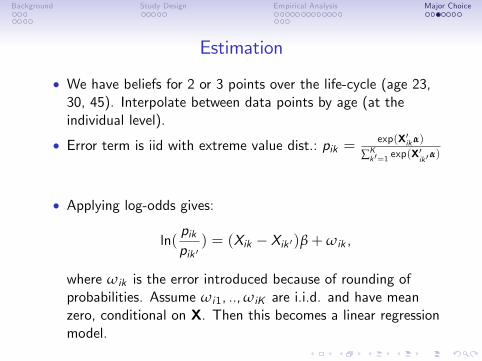
• We have beliefs for 2 or 3 points over the life-cycle (age 23,30, 45). Interpolate between data points by age (at theindividual level).
• Error term is iid with extreme value dist.: pik =exp(X′ikα)
∑Kk ′=1 exp(X
′ik ′α)
• Applying log-odds gives:
ln(pikpik ′) = (Xik − Xik ′)β+ωik ,
where ωik is the error introduced because of rounding ofprobabilities. Assume ωi1, ..,ωiK are i.i.d. and have meanzero, conditional on X. Then this becomes a linear regressionmodel.

Background Study Design Empirical Analysis Major Choice
Model EstimatesMales Females
Disc Own Lifetime Earnings 0.506*** 0.400***
Disc Spouse’s Lifetime Earnings 0.0579 0.115*
Prob of marriage (age 23-35) -0.132 0.329
Prob of marriage (age 36-60) -0.719 -0.083
Exp num of children (age 23-35) 0.186 0.382***
Exp num of children (age 36-60) -0.291 -0.357**
Ability rank (α6) 0.0233*** 0.0281***
Number of individuals 176 317Number of observations 352 634∗∗∗,∗∗,∗ denote sig at the 1%, 5%, and 10% levels.

Background Study Design Empirical Analysis Major Choice
Model Fit
Observed Prob Predicted Prob
MalesScience/Business 66.92% 65.12%Humanities 30.05% 25.4%No Degree 3.22% 9.48%
FemalesScience/Business 48.08% 54.57%Humanities 49.94% 34.22%No Degree 2.16% 11.21%

Background Study Design Empirical Analysis Major Choice
Decomposition
Base Earnings Ability Marriage Sp Earnings FertilityM F M F M F M F M F
Average ProbabilitySci/Bus. 0.33 0.69 0.61 0.67 0.52 0.66 0.51 0.66 0.54 0.65 0.47Hum. 0.33 0.23 0.29 0.24 0.37 0.24 0.38 0.24 0.36 0.25 0.46No Deg. 0.33 0.08 0.10 0.10 0.11 0.11 0.11 0.10 0.10 0.10 0.07
% change from previous col.Sci/Bus. 105.7 82.9 -2.8 -14.3 -1.4 -1.5 1.1 5.4 -2.0 -12.7Hum. -30.3 -12.6 1.7 27.1 0.4 1.4 -0.4 -3.2 7.6 25.9No Deg. -75.1 -70.0 18.1 9.0 8.2 1.8 -5.7 -14.4 -5.0 -26.3
Beliefs about spousal earnings and, in particular, expected fertilityhave large impacts on females’major choices.

Background Study Design Empirical Analysis Major Choice
Conclusion
• Students perceive different returns to HK investments in thelabor and marriage market.
• returns differ by college versus no college; science versushumanities majors
• substantial heterogeneity in ex ante beliefs
• Evidence of students anticipating future outcomes correctly(though perfect foresight is rejected)
• These beliefs about "family" are incorporated in a lifecyclemodel of HK investments
• perceptions regarding future family aspects (marriage, fertility,spousal quality) matter for college major choice