1

How much does geography influence language variation?

John Nerbonne (University of Groningen)

Abstract

This paper proceeds from a quantitative perspective and applies measurements of

linguistic difference to obtain characterizations of the aggregate relations among

varieties in entire language areas. From there it is a small step in quantitative

methodology to ask how much geographic distance influences (aggregate) linguistic

differences, applying a regression design. The paper goes on to contrast the degree to

which a very bare concept of geography, just distance, competes with a more

complicated one, involving areas or regions, in explaining the aggregate linguistic

differences among language varieties. The data is taken from dialect atlases and

various other collections, and the linguistic distance is measured using a variant of

Levenshtein distance, which has been demonstrated to be valid with respect to dialect

speakers’ judgments of linguistic difference. Pure geographic distance models account

for between 14% and 38% of the variation found in the data in straightforward

regression designs. The alternative to pure distance models involves dialect areas,

which we examine on the basis of the independently established dialect areas in

Wrede’s famous map of German dialect areas, adding dialect divisions as categorical

independent variables to assess their explanatory value. This increases the explained

variation from 32% to 45% in the German dialect dataset, indicating that geography is

indeed structured more complexly than simple distances, and also that geography

influences linguistic variation deeply.

1. Introduction

Two insights about language variation are standard and uncontroversial, first that

languages may vary in many ways and second, that nearby language varieties are

generally – but not always – more similar than distant ones. Dialectometry supports

the measurement of linguistic similarity and its inverse, linguistic difference or

distance, in various forms and therefore satisfies a prerequisite for determining the

degree to which geography influences language variation, a line of investigation that

is effectively closed to research traditions that shun measurement in favor of

cataloguing differences. The present paper shows how dialectometry arrives at

measurements and proceeding from these, how the influence of geography on

language variation may be ascertained through regression designs. In addition to this,

two notions of geography are contrasted, one in which the linguistic differences

between varieties is compared to the geographic distance between them (including

derivatives of distance such as travel time), and another, in which sites are partitioned

into areas. We can measure the contribution of areas in the same sort of regression

design used to gauge the influence of geographical distance, and, finally we may

examine a combination of the influence of distance and areas. We close with some

reflections on the ways in which we have conceptualized geography and some

speculation on the effect of modern communication technology, asking whether space

as we have conceptualized it here is likely to continue to be as influential in the future

as it has been in the past.

2

2. Quantitative Dialectology

Dialectometry, or quantitative dialectology, has arisen to solve several problems that

existed in traditional dialectology (Goebl 1986) – in particular, the concrete problem

of “non-overlapping isoglosses”, or more generally, the problem of identifying

geographical structures underlying the distribution of linguistic features. The crux of

the dialectometric solution has been to aggregate over many linguistic features before

seeking geographic interpretation. Goebl speaks suggestively here of the

dialectometer “condensing” (verdichten) linguistic atlas data. In addition to opening

new avenues in which to seek dialect areas (or dialect continua), dialectometry

likewise introduces replicable procedures into the study of dialects and provides a

basis on which the research may seek more abstract regularities or “laws” (Nerbonne

2009). The present essay is concerned primarily with the latter task, that of

formulating more general principles in language variation.

Some simple ways of measuring language similarities are remarkably

effective. Séguy (1971) simply examined the lexical realization of a set of concepts

and counted how often there was agreement and how often disagreement. In later

work he extended this technique by examining linguistic differences not only in word

choices, but also in pronunciation, morphology and syntax.

A slightly more complex analysis is useful to gauge differences in the

pronunciation of words as these are recorded in dialect atlases, i.e. in the form of

phonetic transcriptions. Levenshtein distance counts both the number of substitutions

needed to transform one transcription into another, as well as the numbers of

insertions and deletions, always seeking the minimum number necessary (Nerbonne

and Heeringa 2009). We illustrate the effect of the procedure on two Dutch

pronunciations of melk (the word for ‘milk’), namely Frisian [mɔəlkə] (Grouw) and standard Dutch [mɛlək] (Delft). On the one hand one may examine the operations

needed to map one pronunciation to another:

m ɔ ə l k ə delete ə m ɔ l k ə replace ɔ by ɛ m ɛ l k ə delete ə m ɛ l k insert ə m ɛ l ə k

Or, on the other hand, we may equivalently inspect the alignment induced by this

process:

m ɔ ə l k ə

m ɛ l ə k

1 1 1 1

There are several advantages to using Levenshtein distance to measure the distance

between transcriptions as opposed to collecting categorical features from dialect data

collections (Nerbonne et al. 2010: 42–43). First, using Levenshtein distance automates

a larger part of the process of analyzing dialect atlas data, obviating in particular the

need for the researcher to extract categorical differences by hand. Second, we increase

3

the amount of data compared by nearly an order of magnitude, as we effectively

compare each word at each segment position. A list of one hundred words thus

typically yields about 500 segment comparisons. Third, and related to the second,

using all of the segments of transcribed words means that fewer words suffice for

reliable assessments of the dialect distances between sites. Typically, thirty to forty

transcribed words are sufficient. Fourth, and related to the last two, the use of

Levenshtein distance involves comparing all the segments in the data collected, and

therefore a large number of segments that happen to be in words that were chosen to

illustrate dialect differences This means the data that is analyzed was effectively

collected in a manner closer to the sort of random data selection that is customary in

corpus linguistics and generally recommended in statistical procedures. . About 80%

of the segments subject to analysis were collected only because they happen to occur

in a word with an “interesting” segment. So 20% was selected intentionally, and 80%

unintentionally.

In all of the data sets we examine below, we measure the pronunciation

difference of every pair of corresponding words (phonetic transcriptions), typically

about one hundred words, in each pair of sites, often thousands (of pairs of sites), in

the collection using Levenshtein distance. We take the site difference then to be the

average pronunciation distance per word pair, ignoring in this way the occasional

cases in which data is missing. We then follow Heeringa and Nerbonne (2001) in

applying a simple regression design to the aggregate distances thus assayed, using the

geographic distance between sites as the independent variable and the aggregate

pronunciation distances as the dependent variable.

Given that the present contribution is intended for a volume on language and

space, it is worth pausing to reflect explicitly on why as simple a spatial or geographic

concept as distance plays so central a role in the theorizing. To begin, let us forswear

any interest in the physical properties of space, which we imagine having no influence

on speech patterns or perceptions (not even in virtue of the transmission of the sound

waves). But as Bloomfield (1933, Chap.3.4 et passim) notes, speakers adjust their

speech regularly for their speech partners, leading him to hypothesize that linguistic

habits would likely follow the lines of the densest communication. Space or

geography, as we theorize about it here, is therefore a social concept interesting for

the indications it suggests about where people are communicating with one another.

We suppose that people are also less likely to communicate if they live further away

from each other than if they live close to each other, that is, in the usual case. This is

the basis for examining the relation between simple distance and linguistic similarity.

We do not suppose at all that distance is the only spatial or geographic influence on

the similarity of speech habits (see further), but we examine it first, as it is very basic

to the influence geography has on speakers.

The above, Bloomfieldian view is adopted here for its simplicity. It may seem

to imply that variation inevitably diffuses only in order to facilitate communication

with others, but I do not attribute this view to Bloomfield. As we know, in fact,

variation also arises as a means for a speaker to differentiate himself or herself from

others, and this sort of variation also diffuses. We shall not distinguish the two

different sorts of changes in speech habits, those motivated essentially by

accommodation and those motivated by a wish to assert differentiation. This

perspective on linguistic variation will be ignored in the rest of this essay as I do not

see how it would figure in a spatial or geographic model.

4

We pursue a second step only in the case of one data set, the German set (see

below). In this second step we complicate the simple regression design by including

several more independent variables, in addition to the simple distances just described,

namely a series of “dummy” binary variables which take the value one (‘1’) whenever

two sites under comparison originate from two specific, different, a priori-defined

dialect areas (e.g. the Bavarian area in Germany and the Alemannic German

Southwest), and zero (‘0’) otherwise. This procedure follows a suggestion by

Shackleton (2007, 2010) and is motivated by the wish to investigate whether dialect

areas independently contribute to pronunciation distance – over and above the sheer

distance between the sites that would be accounted for in the simpler design.

3. Data and analysis

In this section we describe the data on which our analyses are based, reporting at the

same time on the regression analyses seeking to explain aggregate pronunciation

distance based on geographic distance. We turn to the potentially different

contribution that might be made by areal distinctions in a following section.

We note here that our use of aggregate pronunciation difference (or

equivalently, average differences) naturally tends to inflate the correlation coefficients

reported below. If we examined the individual word pronunciations, the correlation

coefficients would drop substantially. The focus on the aggregate difference has long

been standard in quantitative dialectology (see the remarks on “condensing” data

above), but the deeper justification for using aggregate measures is that we are

interested in the properties of linguistic varieties, i.e. the overall speech habits in a

community, and not merely the properties of individual words.

3.1. Data and distance analysis

We compare six different dialect data collections, using the same material presented

in Nerbonne (2010). That paper focused on the sub-linear (normally logarithmic)

growth of average phonetic distance as a function of geographic distance, while the

present paper focuses on the degree to which variation is explained via geography,

including geographical distance but also areal partition. Because we have published

focused papers on each of the data sets we use, the descriptions below are somewhat

summary; interested readers are referred to the original papers.

Alewijnse, Nerbonne, van der Veen and Manni (2007) used pronunciation data

from Bantu data collected in Gabon by researchers from the Dynamique du Langage

project (http://www.ddl.ish-lyon.cnrs.fr/) in Lyon. Since the Gabon Bantu population

consisted of migratory farmers until recently, it might be expected to show a different

influence of geography on linguistic variation. The data involve broad phonetic

transcriptions of 160 concepts taken from 53 sampling sites. Tone was not analyzed as

the Bantu experts were skeptical about how reliably it had been recorded and

transcribed. The geographic locations recorded were those provided by native speaker

respondents, but they should be regarded in some cases as “best guesses” considering

how mobile the population has been (over long periods of time). The pronunciation

differences were analyzed using the procedure sketched in Section 2 above, and these

correlate moderately with logarithmic geographic distances (r = 0.469).

5

Houtzagers, Nerbonne and Prokić (2010) obtained data on Bulgarian dialects

from Prof. Vladimir Zhobov’s group at the St. Clement of Ohrid’s University of

Sofia. The research analyzed broad phonetic transcriptions of 156 words from 197

sampling sites in Bulgaria. Palatalized consonants, which are phonemic in Bulgarian,

are represented in the data, but stress is not. The pronunciation difference

measurement described above was applied, where alignments were constrained to

respect syllabicity, meaning that vowels were only allowed to align with vowels, and

consonants only with consonants. Because of the long Ottoman occupation of Turkey

(until 1872), its patterns of variation may be atypical, but the correlation of

pronunciation and logarithmic geographic distance was measured at r = 0.488.

Nerbonne and Siedle (2005) obtained data from the Deutscher Sprachatlas in

Marburg (http://www.uni-marburg.de/fb09/dsa/). The pronunciations of 186 words

had been collected at 201 sampling sites for the project Kleiner Deutscher Lautatlas.

A team of phoneticians transcribed the data narrowly; each word was transcribed

twice independently and disagreements were settled in consultation so that there was

consensus about the results. The pronunciation differences were measured using

Levenshtein distance, where alignments were constrained as above to respect

syllabicity. Logarithmic geographic distance correlates strongly with pronunciation in

this data set (r = 0.566).

Kretzschmar (1994) reports on the LAMSAS (Linguistic Atlas of the Middle

and South Atlantic States) project, conceived and carried out mainly by Hans Kurath,

Guy Lowman and Raven McDavid in the 1930s and again in the 1950s and 1960s.

The data is publicly available at http://hyde.park.uga.edu/lamsas/. Due to differences

in fieldworker/transcriber practices, we analyze only the 826 interviews which Guy

Lowman conducted in the 1930s involving 151 different response items. LAMSAS

used its own transcription system, which we converted automatically to X-SAMPA

for the purpose of this analysis. This analysis we conducted using a variant of the

measurements above. Nerbonne (to appear) describes some aspects of the analysis in

more detail, in particular the degree to which phonological structure is present. Since

the area of the present U.S. has only been English speaking for the last several

centuries, it may retain traces of migration disturbance in the geographic distribution

of linguistic variation. We nonetheless measured a strong correlation between

pronunciation and geographic distance after applying a logarithmic correction to the

latter (r = 0.511).

Wieling, Heeringa and Nerbonne (2007) analyze the data of the projects

Morphologische Atlas van Nederlandse Dialecten (MAND) and Fonologische Atlas

van Nederlandse Dialecten (FAND) (Goeman and Taeldeman 1996). In order to

avoid a potential confound due to transcription differences, Wieling et al. analyze

only the data from the Netherlands, and not that of Flanders. The former included 562

linguistic items from 424 varieties. Since the Netherlands comprises only 40.000 km2,

the MAND/FAND is one of the densest dialect samplings ever. The pronunciation

differences were measured using the technique described above, where alignments

were constrained to respected syllabicity. Pronunciation distance correlates strongly

with the logarithm of geographic distance (r = 0.622).

Gooskens and Heeringa (2004) analyze the variation in 15 Norwegian versions

of the fable of the International Phonetic Association, “The North Wind and the Sun”,

making use of material from http://www.ling.hf.ntnu.no/nos/. The material was again

analyzed using the pronunciation difference measurements explained above. David

6

Britain (2002) urges dialectologists to examine critically the underlying conceptions

of geography they emply. Interestingly from this point of view, Gooskens (2004)

compares two geographic explanations of the linguistic differences, one based on “as

the crow flies” distances, and another based on the (logarithmic) travel time estimates

of the late nineteenth century, showing an improvement in correlation (from r = 0.41

to r = 0.54). The motivation for examining the two operationalizations was naturally

that travel time is expected to be the better reflection of the chance of social contact,

i.e. Bloomfield’s “density of communication”.

Figure 1. Pronunciation differences in Bantu, Bulgaria, Germany, the US Eastern

Seaboard, Netherlands and Norway as functions of geographic difference. In each

case a logarithmic regression line is drawn. Please note that the vertical y-axes have

not been calibrated.

7

We conclude from this section that there is a simple and measurable influence

which geographic distance exerts on aggregate linguistic differences. Figure 1

summarizes the six data sets discussed above and sketches the regression line in each

case. It is an empirical finding, not a theoretical prediction, that geography accounts

for 16% to about 37% of the linguistic variation in these data sets (100 × r2). We note

that the potential disturbances caused by migration, occupation, and recent settlement

appear insubstantial enough in the cases examined so as not to disturb the overall

tendency.

For readers of this volume who may not be as familiar with regression

analyses as they would like, it is worth emphasizing some relevant, well-known facts

about regression analyses in order to fend off misunderstandings. First, what counts as

a “strong correlation” varies from one field of investigation to another, but many

research fields use r > 0.5 as a cutoff. Second, the square of the correlation coefficient

is the fraction of variance (variation) accounted for by the independent variables in the

regression analysis. Given that language variation is highly complex, and that we have

examined a substantial amount of it (and not merely some selected variables), one

cannot expect extremely high levels of correlation (or of the derived percentage of

explained variance). Third, obtaining a correlation coefficient of r = 0.6 (and thereby

accounting for 36% of the variation in a data set) means that a great deal of variation

is still unaccounted for, and so there is lots of work to be done. Fourth, we want to

keep in mind that saying, e.g., that distance accounts for 36% of the variation in a data

set does not mean that another, alternative explanation could not account for more

than 64%. This is eminently possible, in particular, where distance might correlate

with an alternative explanation to some degree, for example if there were a way to

measure the ease of communication between settlements, or the strength of the ties

that bind the communities. Fifth, we advisedly use the mean pronunciation distance

between varieties as our dependent variable, and not, e.g. the pronunciation distance

between the pronunciations of a particular word for the simple reason that we are

interested in the entire variety spoken at a given site. As we noted above, correlations

involving a mean are inevitably inflated, as they remove a significant amount of noise

from the data. Statisticians have introduced the term “ecological fallacy” for steps in

reasoning that infer properties of individuals (words) from the properties of

aggregates (sites) (Agresti and Franklin 2009). This study is not guilty of the

ecological fallacy because, as we noted at the beginning of this section (Sec. 3), we

focus on the distances between entire varieties, and not on the distances of individual

words. But the caution is appropriate: we can explain about 30% of the variation

among varieties, but not 30% of the variation in individual words.

3.2. Areal Analysis

There are several reasons to look beyond distance as explicans in variationist

linguistics. Reflecting on its introduction above, we recall that we were inspired by

Bloomfield’s (1933) notion of “density of communication”. But if the density of

communication influences language variation, then there is good reason to think that

we might gauge this influence not only via distance but perhaps also through other

phenomena that might provide some purchase on communicative density.

8

One such phenomenon is dialect area, the basis of undoubtedly the most

popular visualization of geographic influence on language variation – that of dialect

maps showing a partition of a language area into non-overlapping dialect areas. In

Map 1 we present Wrede’s division of Germany into six major areas.1 Given this map

it is natural to ask whether language variation is less a matter of continuous variation

along the dimension of distance between sites, and rather more a matter of sites

participating in a partition of relatively homogeneous areas. The quantitative

perspective allows us to compare the influence of distance (see above) with that of

area.

1 Niebaum and Macha (2006: 38) explain that Wrede’s map was published posthumously in 1937 by

Bernhard Martin as Deutscher Sprachatlas, 9th

Lieferung, Karte 56.

9

Map 1. Wrede’s (1937) atlas of German dialects has been taken here in order to use an

authoritative source as a hypothesis. We shall refer to the areas (clockwise, from top

left) as the northwest, the northeast, Saxony, Bavaria, the southwest, and the

Palatinate. The dark lines separate Wrede’s areas while the divisions in coloring

depend on the automatic “tiling” done around data collection sites. There’s a slight

mismatch when sites practically lie on borders.

4. Analysis

We focus in this section on the German data, examining the effect of geographic

distance through a regression design in which both bare distance but also areal

10

differences are used as independent variables. Naturally they are both examined for

their effect on the dependent variable, linguistic distance.

In order to evaluate the influence of area quantitatively, we shall introduce

variables which indicate when two sites are in two specific, different areas. For

example, we shall introduce a variable “Southwest-vs-Bavarian” which has the value

‘1’ if, and only if, one site in question is from the southwest in Wrede’s map and the

other from Bavaria. It has the value zero in every other case, i.e. when both sites are in

the southwest, when they are both in Bavaria, when one site is in the southwest or

Bavaria and the other is somewhere else, and also when both sites are outside of both

areas. Note that there are six areas, meaning that we shall need to introduce fifteen

such variables, one for each pair of areas.

Shackleton (2007: 61ff) was the first to suggest analyzing the effects of dialect

areas in this way, using it to show the significance of dialect areas he obtained by

clustering distance measures. Note that cluster differences are derived from linguistic

distance measures, meaning that they clearly may not be regarded as statistically

independent. Without criticizing Shackleton’s work, let us note that some circularity

may be lurking in the regression analysis that uses cluster differences derived from

linguistic differences to explain the same set of linguistic differences. Let us therefore

examine here the areal differences shown in Wrede’s independently derived map. The

analysis here differs only in that we have chosen not to use a derivative of the

linguistic distance measure as its own explicans. Instead, we examine the effect of an

independently proposed set of areal differences, Wrede’s. Ignoring that difference, our

regression analysis follows Shackleton’s in technical design. The fifteen areal

differences variables are added to the multiple regression design.

The comparison of bare distance versus areas as explanatory variables may be

regarded as the quantitative form of the old question of whether dialects should be

regarded as organized spatially as continua or as areas, i.e., discrete partitions of

relatively uniform sets of sites. If the continuum view is correct, areal differences

should explain nothing in models in which bare distance is included. But if on the

other hand the areal view is sufficient, then the areal variables should turn out to be

significant, and bare distance should play no explanatory role. Naturally there is also

a “third” view which acknowledges that gradual variation is consistent with both

constant rates of additional variation as well as rates that may change rather abruptly.

If linguistic differences increase constantly, we obtain a perfect continuum. If, on the

other hand, the rate of differentiation changes abruptly, we obtain a situation in which

both the continuum and the areal views have some validity.

As we introduce such variables indicating areal difference, we nonetheless

need to exercise some caution. The more areas we distinguish (and therefore the more

variables we introduce), the better the chance of seeing a statistical significant effect

for at least some areal differences. In the most extreme (and uninteresting) case, in

which a variable were introduced for each pair of sites, the linguistic distance could be

predicted perfectly. But as long as we examine only a relatively small number of

areas, the question of whether bare distance or areal distinctions are the better

predictors is genuine. As long as the number of areas distinguished is low, we expect

to see that bare distance remains significant – at least within the large areas, which,

after all, are not completely uniform.

11

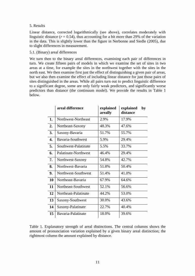
5. Results

Linear distance, corrected logarithmically (see above), correlates moderately with

linguistic distance (r = 0.54), thus accounting for a bit more than 29% of the variation

in the data. This is slightly lower than the figure in Nerbonne and Siedle (2005), due

to slight differences in measurement.

5.1. (Binary) areal differences

We turn then to the binary areal differences, examining each pair of differences in

turn. We create fifteen pairs of models in which we examine the set of sites in two

areas at a time, for example the sites in the northwest together with the sites in the

north east. We then examine first just the effect of distinguishing a given pair of areas,

but we also then examine the effect of including linear distance for just those pairs of

sites distinguished in the areas. While all pairs turn out to predict linguistic difference

to a significant degree, some are only fairly weak predictors, and significantly worse

predictors than distance (the continuum model). We provide the results in Table 1

below.

areal difference explained

areally

explained by

distance

1. Northwest-Northeast 2.9% 17.9%

2. Northeast-Saxony 48.3% 47.6%

3. Saxony-Bavaria 51.7% 55.7%

4. Bavaria-Southwest 5.9% 29.4%

5. Southwest-Palatinate 5.5% 33.7%

6. Palatinate-Northwest 46.4% 29.4%

7. Northwest-Saxony 54.8% 42.7%

8. Northwest-Bavaria 51.8% 50.4%

9. Northwest-Southwest 51.4% 41.0%

10 Northeast-Bavaria 67.9% 64.6%

11 Northeast-Southwest 52.1% 56.6%

12 Northeast-Palatinate 44.2% 53.0%

13 Saxony-Southwest 30.0% 43.6%

14 Saxony-Palatinate 22.7% 40.4%

15 Bavaria-Palatinate 18.0% 39.6%

Table 1. Explanatory strength of areal distinctions. The central columns shows the

amount of pronunciation variation explained by a given binary areal distinction; the

rightmost column the amount explained by distance.

12

We should add that our measurements cannot be interpreted to mean, e.g., that

there is no Bavaria-southwest distinction (Table 1, line 4), but only that Wrede’s

border is not a worthwhile distinction to be drawn for this dataset, which, of course,

was collected nearly a century after Wrede’s. This conclusion also assumes that we

are examining the sites together with the distances between them, and that we are

focusing on the question of whether Wrede’s border should also be drawn to partition

the set of sites in the south of Germany. Other researchers are free to attempt to show

that another border distinguishing the west and the east in the south is a a more

explanatory one. Unless they draw the border in a very different fashion, they are

unlikely to be successful in this endeavor of course, as they can only obtain different

results to the degree that they distinguish sites differently from the way we have here.

We return to a further discussion of this issue at the end of this section.

If we restrict our attention to areas sharing a border (lines 1-7, 13-14 in Table

1; compare Wrede’s map in Map 1) then we see that the northeast-Saxon border is

slightly more predictive than distance (line 2), and that the border between the

northwest and the more southern areas are massively explanatory (lines 6-7). No

improvement in explained variation is associated with either the east-west border in

the north, nor with any of the borders in the south.

Since this is a paper on methods in dialectology, and not on German

dialectology in particular, we shall not pursue the potentially shocking conclusion

here that, assuming continuum effects due to geographic distance, there are really

only two important German dialect areas: the north (Plattdeutsch) involving the

northeast and northwest on the one hand, and the south on the other, including all the

others (Saxony, Bavaria, the southwest and the Palatinate). What might be shocking

to the Germanist is not that we detect traces of this major division, nor even that it

appears to be the most significant division, but rather that other areas explain rather

little variation. To draw that conclusion with confidence we should need to examine a

range of perturbations of Wrede’s partition of sites, but the conclusion is definitely

suggested by Table 1, where the only distinctions that explain much variation involve

areas from either side of the north-south dividing line. All the other areal divisions

either explain less than distance alone, or only marginally more. If we assume, as

seems reasonable, that distance is the more primary notion of geography (compared to

area), and then ask what further notions are explanatory, then only some of Wrede’s

areas would cross the threshold of utility in explanation.

5.2. Combined models

If we ignore linear distance but include all the binary areal differences, then we find a

somewhat stronger correlation (r = 0.58) than we did for distance alone (r = 0.54),

accounting for 33.8% of the variation in the data. This difference is statistically

significant due to the large number of site pairs involved (20,100 pairs involving the

201 sites), but we shall not dwell on that.

It is a surprising result that the 15 binary variables together explain more of

the variation than the simple distance, vindicating the traditional view in German

dialectology, which is visualized in Wrede’s map, that dialectal space is not a

continuum, but rather influences pronunciations discretely, in virtue of the individual

sub-spaces (areas) to which sites belong. We also note that not every areal distinction

influences linguistic differences significantly in this large model. In particular,

13

Wrede’s distinction between the northwest and the northeast correlates only

insignificantly with linguistic differences (p ≈ 0.36), as does the distinction between

the Palatinate and the southwest (p ≈ 0.24), while the distinction between the

southwest and Bavarian is only borderline significant (p ≈ 0.044). Given our

examination of the pairs of areas above, these results showing insignificance are

hardly surprising.

We also have the option of examining models which combine linear distance

and areal differences, however, and here we see that the traditional view, which we

vindicated above, was also incomplete. Taken together, the two notions of geography

correlate much more strongly with geography (r = 0.69), accounting therefore for

47.2% of the aggregate pronunciation variation in the data. It is straightforward to

interpret this result as indicating that a good deal of variation is not explained by areal

differences, and that some continuum effects persist even with fifteen binary areal

distinctions.

6. Conclusions

The focus of this paper has been the demonstration that quantitative dialectology may

contribute new perspectives to discussions of how language variation and space

interact.

First, we may calculate a measure of the degree to which language variation

depends on space – this is the percentage of explained variance in regression models

such as those presented above.

Second, quantitative dialectology is neutral with respect to the geographical

notions brought to the table, assuming that they may be incorporated into regression

models. This paper has demonstrated how two different conceptions of geography –

linear distance on the one hand versus areal divisions on the other – may be compared

in a quantitative fashion. It is clear that the division into geographic areas is only one

of the organizing geographic concepts that might be evaluated quantitatively. A

second candidate might be political borders, e.g. the case of the U.S.-Canadian border,

which Boberg (2000) has argued to define a linguistic barrier. A third might be the

radially shaped diffusion from centers of population, trade or government, which are

related to the existence of dispersed “relic areas” (Chambers and Trudgill 1998:

94,119). Other candidates are the “staggered” patterns (Niebaum and Macha 2006:

105) of distributions resulting from diffusions of similar, but not identical dynamics,

or perhaps the ribbon-shaped diffusion along important trade and travel routes. Some

such patterns will not be analyzed successfully without some clever additions to the

methodology I have sketched above, since it is not always clear how to characterize

these structures in a way amenable to quantitative analysis, but the effort will be

worthwhile.

Third, we have not just suggested the feasibility of mixed forms of geographic

influence, but more importantly we have demonstrated that geography in fact is

influential in a mixed form, involving both distance and area in a very well studied

language area such as Germany.

14

7. Reflections on Geography

In all of what is written above, geography – whether geographic distance or as the

basis of an areal division among varieties – certainly should not be understood as a

physical influence on language variation, but rather as a useful reification of the

chance of social contact. Accordingly, we regard space as something which promotes

or discourages social contact, and which does so by virtue first of the distances which

settlements may be from one another, and second, by the regions which settlements

may co-occupy (or fail to co-occupy). With respect to the first, we note that a space

which defines travel times, rather than kilometers of remoteness of positions, may

function better than space as it is normally conceived, as the temporal notion

influences the chance of social contact even more directly than the geographical

notion. Recall Gooskens (2004), discussed above. With respect to the second, we

hypothesize that regions are influential to the degree to which they represent relatively

closed social networks. In speculating this way I do not mean to suggest that the

borders of the German areas sketched by Wrede were ever impermeable for the

purposes of communication, only that communication tended to involve people within

a single area more than people from two different areas. This, at any rate, would be

the Bloomfieldian line.

Space proves to be massively influential from this perspective, but one should

not imagine that its influence is inescapable. Where modern, interactive means of

communication support intimate, extended exchange, where interlocutors have the

opportunity to appreciate not only what each other is saying, but also how it is being

said, and where occasionally adopting one another’s speech habits can be appreciated,

one might expect such interactions to influence patterns of language variation, at least

in the short term. In this case one might also expect notions like the difficulty of

communicative interaction to play a role in predicting linguistic dissimilarity much

like that now played by physical remoteness. But let us note at the same time that

communities that are defined by occasional communication (lots of blogging, net lists,

twitter, etc.), and which are difficult to gauge with respect to their language variety

might be characterized by changes that reflect brief accommodation (linguistic

registers) rather than by longer term changes in language habits. The jury is still out

on whether the newest generation of communication technology will influence

language variation more permanently.

References

Agresti, Alan and Christine Franklin 2009 Statistics. The Art and Science of

Learning from Data. (2nd

ed.) Upper Saddle River, New Jersey: Pearson.

Alewijnse, Bart, John Nerbonne, Lolke van der Veen and Franz Manni 2007 A

Computational Analysis of Gabon Varieties. In: Petya Osenova et al. (eds.),

Proceedings of the RANLP Workshop on Computational Phonology, 3–12. Workshop

at Recent Advances in Natural Language Processing (RANLP), Borovetz.

Bloomfield, Leonard 1933 Language. New York: Holt, Rinehart and Winton.

Boberg, Charles 2000 Geolinguistic diffusion and the U.S.-Canada border.

Language. Variation and Change, 12(1):1–24.

15

Britain, David 2002 Space and Spatial Diffusion. In: Jack K. Chambers, Peter

Trudgill and Natalie Schilling-Estes (eds.), The Handbook of Language Variation and

Change, 603–637. Oxford: Blackwell.

Chambers, Jack K. and Peter Trudgill 1998 Dialectology. Cambridge:

Cambridge University Press.

Goebl, Hans 1986 Muster, Strukturen und Systeme in der Sprachgeogrpahie.

Mondo Ladino 10: 41-70.

Goeman, Anton and Johan Taeldeman 1996 Fonologie en morfologie van de

Nederlandse dialecten. Een nieuwe materiaalverzameling en twee nieuwe

atlasprojecten. Taal en Tongval, 48: 38–59

Gooskens, Charlotte 2004 Norwegian Dialect Distances Geographically

Explained. In: Britt-Louise Gunnarson, Lena Bergström, Gerd Eklund, Staffan

Fridella, Lise H. Hansen, Angela Karstadt, Bengt Nordberg, Eva Sundgren and Mats

Thelander (eds.), Language Variation in Europe: Papers from ICLaVE 2, 195–206.

Uppsala: Uppsala University.

Heeringa, Wilbert and John Nerbonne 2001 Dialect Areas and Dialect

Continua. Language Variation and Change 13: 375–400.

Houtzagers, Peter , John Nerbonne and Jelena Prokic 2010 Quantitative and

Traditional Classifications of Bulgarian Dialects Compared. Scando-Slavica 59(2):

29–54.

Kretzschmar, William A. (ed.) 1994 Handbook of the Linguistic Atlas of the

Middle and South Atlantic States. Chicago: The University of Chicago Press.

Nerbonne, John 2009 Data-Driven Dialectology. Language and Linguistics

Compass 3(1): 175–198.

John Nerbonne 2010 Measuring the Diffusion of Linguistic Change

Philosophical Transactions of the Royal Society B: Biological Sciences, 365: 3821–

3828.

Nerbonne, John to appear Various Variation Aggregates in the LAMSAS

South. In: Catherine Davis and Michael Picone (eds.), Language Variety in the South

III, Tuscaloosa: University of Alabama Press

Nerbonne, John and Wilbert Heeringa 2009 Measuring Dialect Differences.

In Jürgen Erich Schmidt and Joachim Herrgen (eds.), Theories and Methods, 550–

567. (Language and Space Vol. 1) Berlin: Mouton De Gruyter.

Nerbonne, John, Jelena Prokić, Martijn Wieling and Charlotte Gooskens 2010Some

Further Dialectometrical Steps. In: Gotzon Aurrekoetxea and Jose L. Ormaetxea

(eds.), Tools for Linguistic Variation Bilbao. 41–56. Supplements of the Anuario de

Filología Vasca "Julio Urquijo", LIII.

Nerbonne, John and Christine Siedle 2005 Dialektklassifikation auf der Grundlage

aggregierter Ausspracheunterschiede. Zeitschrift für Dialektologie und Linguistik

72(2): 129–147.

Niebaum, Hermann and Jürgen Macha 2006 Einführung in die Dialektologie

des Deutschen, 2nd, revised ed. Tübingen: Niemeyer.

16

Shackleton, Robert G., Jr. 2005 English-American speech relationships: A

quantitative approach. Journal of English Linguistics, 33: 99–160.

Shackleton, Robert G., Jr. 2010 A Quantitative Examination of English-

American Speech Relationships. Ph.D. thesis, University of Groningen.

Séguy, Jean 1971 La relation entre la distance spatiale et la distance lexicale.

Revue de Linguistique Romane 35(138): 335–357.

Wieling, Martijn, Wilbert Heeringa and John Nerbonne 2007 An Aggregate

Analysis of Pronunciation in the Goeman-Taeldeman-van Reenen Project Data. Taal

en Tongval 59(1): 84–116.