How does FTIR work?

I receive a steady trickle of enquiries along this line and some of them have been included in Dear Readers [only the ones that have some general interest!]. It is clear from some of the enquiries that many (perhaps most) of you don’t really know how your FTIRs work. Oh I know you’ve all seen the one paragraph description of an interferometer, but very few pieces I have seen tell you how it’s done – what goes on under the cover! Now I’m the sort of idiot who does (or rather ‘used to’) do his own car repairs and I like to know the details. So, I thought I would write a piece for you on this fascinating subject.

The basic idea

The building blocks of an F-T are very different from the predecessor, the double beam (diffraction) infrared spectrometer. In an F-T you have the chain –

Source Interferometer   Sample   DetectorEach building block varies from manufacturer to manufacturer but basically they all obey the same laws of physics. I can’t be exhaustive, but I will try to cover most of the bits and pieces used in contemporary instruments.Sources

The easy bit. All the manufacturers use a heated ceramic source. The composition of the ceramic and the method of heating vary but the idea is always the same, the production of a heated emitter operating at as high a temperature as is consistent with a very long life. Historically, people have achieved this objective in almost bizarre ways e.g. using an old fashioned gas mantle, or the Nernst Glower [a device utilising the fact that some ceramics conduct electricity when heated. The Nernst had to be pre-heated and then could be used as a conductor and hence as a hot source – they were tricky to use and unreliable]. These days, the manufacturers tend to go for either a conducting ceramic or a wire heater coated with ceramic. Now, as I explained recently when talking about hot samples in Raman spectroscopy, heated objects emit, the emission occurs at all wavelengths AND the emission at any wavelength increases with temperature. The plots of emission vs. frequency are shown in Figure 1.

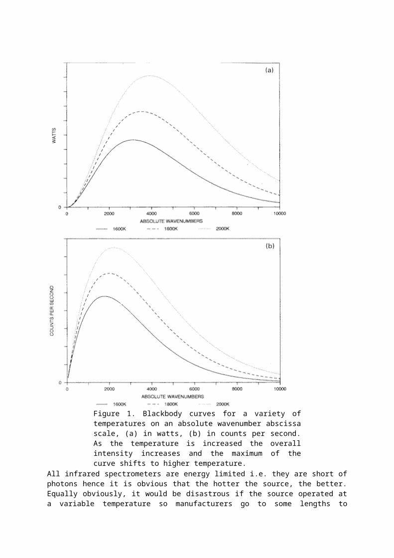
Figure 1. Blackbody curves for a variety of temperatures on an absolute wavenumber abscissa scale, (a) in watts, (b) in counts per second. As the temperature is increased the overall intensity increases and the maximum of the curve shifts to higher temperature.

All infrared spectrometers are energy limited i.e. they are short of photons hence it is obvious that the hotter the source, the better. Equally obviously, it would be disastrous if the source operated at a variable temperature so manufacturers go to some lengths to prevent draughts passing the hot source. This is not as easy as it sounds because air will inevitably convect past the source due to its temperature. Many manufacturers get round this problem by monitoring the source output, using the output signal to control the electrical power in a feed-back loop.

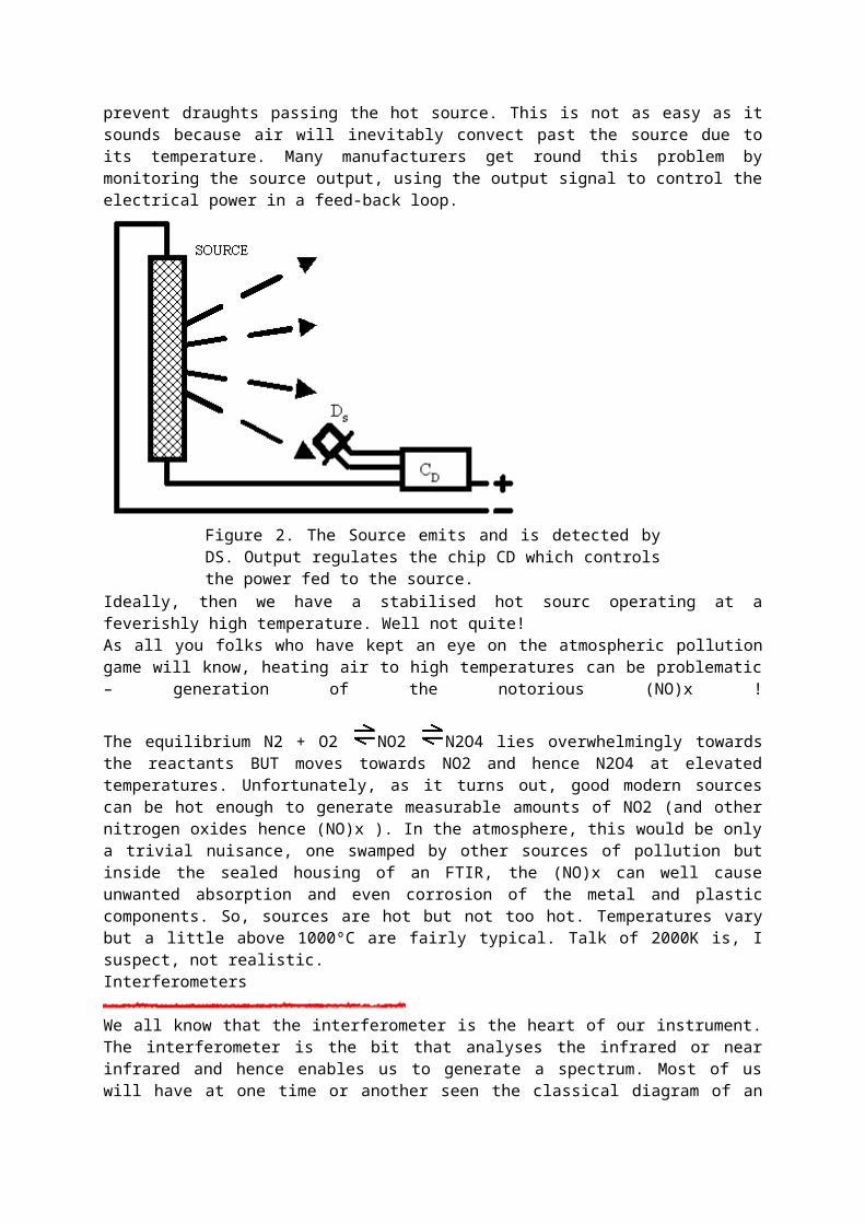
Figure 2. The Source emits and is detected by DS. Output regulates the chip CD which controls the power fed to the source.

Ideally, then we have a stabilised hot sourc operating at a feverishly high temperature. Well not quite!As all you folks who have kept an eye on the atmospheric pollution game will know, heating air to high temperatures can be problematic – generation of the notorious (NO)x !

The equilibrium N2 + O2 NO2 N2O4 lies overwhelmingly towards the reactants BUT moves towards NO2 and hence N2O4 at elevated temperatures. Unfortunately, as it turns out, good modern sources can be hot enough to generate measurable amounts of NO2 (and other nitrogen oxides hence (NO)x ). In the atmosphere, this would be only a trivial nuisance, one swamped by other sources of pollution but inside the sealed housing of an FTIR, the (NO)x can well cause unwanted absorption and even corrosion of the metal and plastic components. So, sources are hot but not too hot. Temperatures vary but a little above 1000ºC are fairly typical. Talk of 2000K is, I suspect, not realistic.Interferometers

We all know that the interferometer is the heart of our instrument. The interferometer is the bit that analyses the infrared or near infrared and hence enables us to generate a spectrum. Most of us will have at one time or another seen the classical diagram of an interferometer and had it explained to us. Let’s go through this again.The classic Michelson Interferometer involves a beam splitter – a component which reflects about ½ of the radiation that hits it and transmits the rest. One bundle of radiation follows one path and the remainder a different path. The two bundles are then recombined and pass out of the device. Now, one path is changed in length allowing radiation to interfere with that following the fixed path. In Figure 3, I show the classical diagram of the Michelson Interferometer.

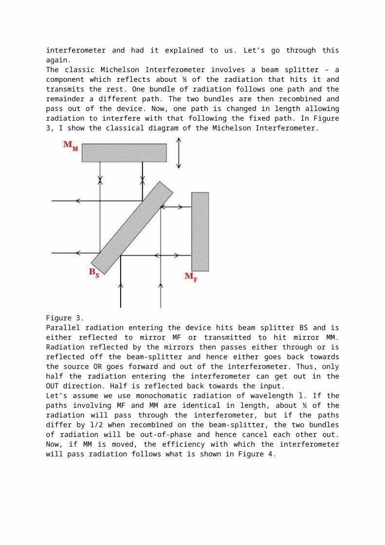
Figure 3.Parallel radiation entering the device hits beam splitter BS and is either reflected to mirror MF or transmitted to hit mirror MM. Radiation reflected by the mirrors then passes either through or is reflected off the beam-splitter and hence either goes back towards the source OR goes forward and out of the interferometer. Thus, only half the radiation entering the interferometer can get out in the OUT direction. Half is reflected back towards the input.Let’s assume we use monochomatic radiation of wavelength l. If the paths involving MF and MM are identical in length, about ½ of the radiation will pass through the interferometer, but if the paths differ by l/2 when recombined on the beam-splitter, the two bundles of radiation will be out-of-phase and hence cancel each other out. Now, if MM is moved, the efficiency with which the interferometer will pass radiation follows what is shown in Figure 4.

Figure 4. If now, we use radiation of 2 wavelengths l1 and l2 the result is shown in Figure 5,

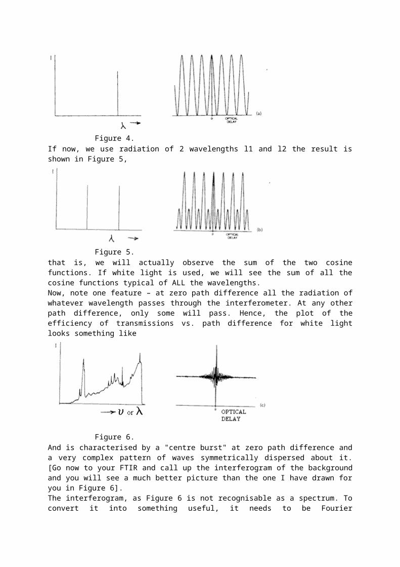
Figure 5. that is, we will actually observe the sum of the two cosine functions. If white light is used, we will see the sum of all the cosine functions typical of ALL the wavelengths.Now, note one feature – at zero path difference all the radiation of whatever wavelength passes through the interferometer. At any other path difference, only some will pass. Hence, the plot of the efficiency of transmissions vs. path difference for white light looks something like

Figure 6. And is characterised by a "centre burst" at zero path difference and a very complex pattern of waves symmetrically dispersed about it. [Go now to your FTIR and call up the interferogram of the background and you will see a much better picture than the one I have drawn for you in Figure 6].The interferogram, as Figure 6 is not recognisable as a spectrum. To convert it into something useful, it needs to be Fourier Transformed. At this stage, all textbooks launch into calculus, but I have always found that students went cross-eyed when I tried, so here is a simple-minded explanation of the Fourier Transform process.Let’s assume the interferogram is digitised and stored in a processor. Now let us also assume that the spectrum we want spans the range 4000 400cm-1 (or in near infrared instruments 12,000 2,500cm-1). If the processor is told to generate a cosine function for radiation frequency 4000cm-1 (wavelength 2.5 µ) it can then search the memorised interferogram for its presence to produce a function F. The search can then be made for radiation of frequency 3999cm-1and so on down to 400cm-1 . The outcome will be the results shown in Figure 7.

Figure 7. Plot of F vs Frequency in cm-1A series of points define how much of the various waveforms are present in the interferogram. Put another way, the FT processor acts as a 'frequency analzyer'. If the computer is then told to join up the points the result is a recognisable spectrum.

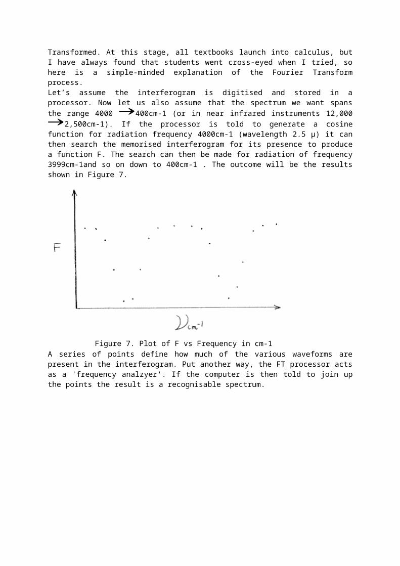
Figure 8. [Now go to your machine and run a spectrum of anything you like at 4cm-1 resolution. Put it up on the screen and then expand the cm-1 axis. Once very well expanded you will see that indeed the spectrum is a series of straight lines joining points].Let us leave the transformation here and come back to it later and then also discuss resolution and other details. Let’s look at real instruments first.Practical Interferometers

Early interferometers (and some persist to this day) use a system identical to that in Figure 1. To make the light parallel, mirror collimators (C) are used and so the instrument looks like Figure 9.

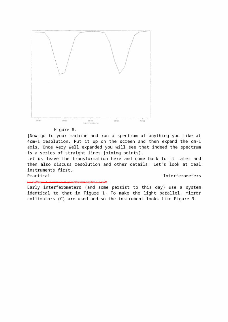
Figure 9. A complete Michelson Interferometer. J= Jacquinot stop, M1= off-axis ellipsiod, M2 & M3= off-axis paraboloids.Note the Beamsplitter BS need not be at 45° to the incoming beam. It rarely is in real instruments,

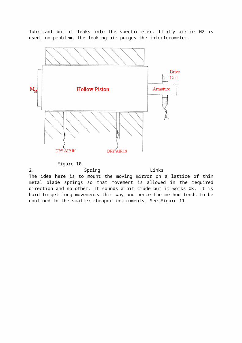
All components are firmly fixed to a base but mirror MM moves backward and forwards on an axis normal to its surface. Clearly, the movement must be smooth, reproducible and involve no wobble or shake. These requirements are hard to achieve and lend to the use of high precision engineering. Two solutions are commonly found –1. Air Bearing Here, a very accurate cylinder houses an equally accurate piston. The latter is ever so slightly smaller than the cylinder and the gap is filled with flowing compressed air. In fact, the piston never touches the cylinder – it floats. A magnetic coil then provides the forward and backward movement. See Figure 10. The air acts as a lubricant but it leaks into the spectrometer. If dry air or N2 is used, no problem, the leaking air purges the interferometer.

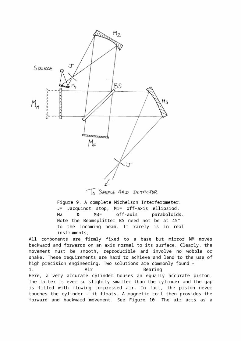
Figure 10. 2. Spring Links The idea here is to mount the moving mirror on a lattice of thin metal blade springs so that movement is allowed in the required direction and no other. It sounds a bit crude but it works OK. It is hard to get long movements this way and hence the method tends to be confined to the smaller cheaper instruments. See Figure 11.

Figure 11. As usual Mm is the moving mirror, A the armature and C the drive coil. The thin springs are S.As drawn, the system won't work. A real system is far too complex to

draw (or rather I chickened out!). Can anyone suggest WHY it won't work? Ed

Whatever method of mirror movement is selected, some shake and wobble is inevitable so some manufacturers have attempted to reduce the problem by using the "corner cube". Imagine a hollow cube made of mirrors. Now cut it in half across its diagonal. Looking into one of the halves you will see -

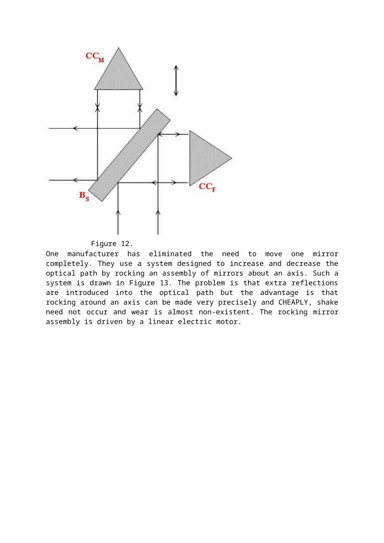
The device has a peculiar property very useful to surveyors and instrument manufacturers. Regardless of the angle at which it is held, light entering the corner cube will be reflected accurately back upon itself – less need to establish or maintain precise alignment! Mirror MM can be replaced by a corner cube and shake and wobble will be much less of a problem than if a plane mirror is used. See below in Figure 12.

Figure 12. One manufacturer has eliminated the need to move one mirror completely. They use a system designed to increase and decrease the optical path by rocking an assembly of mirrors about an axis. Such a system is drawn in Figure 13. The problem is that extra reflections are introduced into the optical path but the advantage is that rocking around an axis can be made very precisely and CHEAPLY, shake need not occur and wear is almost non-existent. The rocking mirror assembly is driven by a linear electric motor.

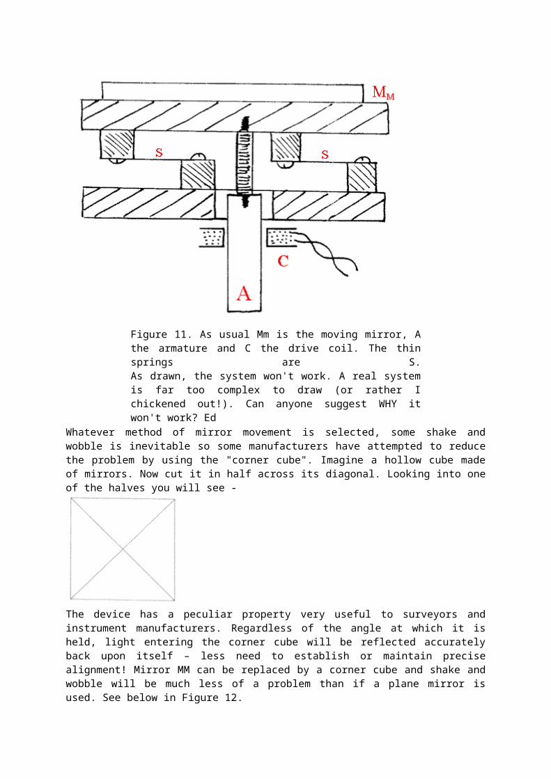
Figure 13. So – we have our interferometer and hence, as we shall see our interferogram. The next problem is to measure the path difference. A ruler is no good, the path difference has to be measured to an accuracy limited only by the precision of the engineering in the interferometer itself. The way this is done is to use the interferometer itself to do the job and to feed it with a source of precisely known wavelength. The He/Ne laser has a wavelength near 632.8nm and is known to very high precision. If a He/Ne laser beam passes through the interferometer, its intensity at the output will generate a superb simple cosine with a peak in intensity every 632.8nm of change in the path difference. How this can be done is shown below in Figure 14.

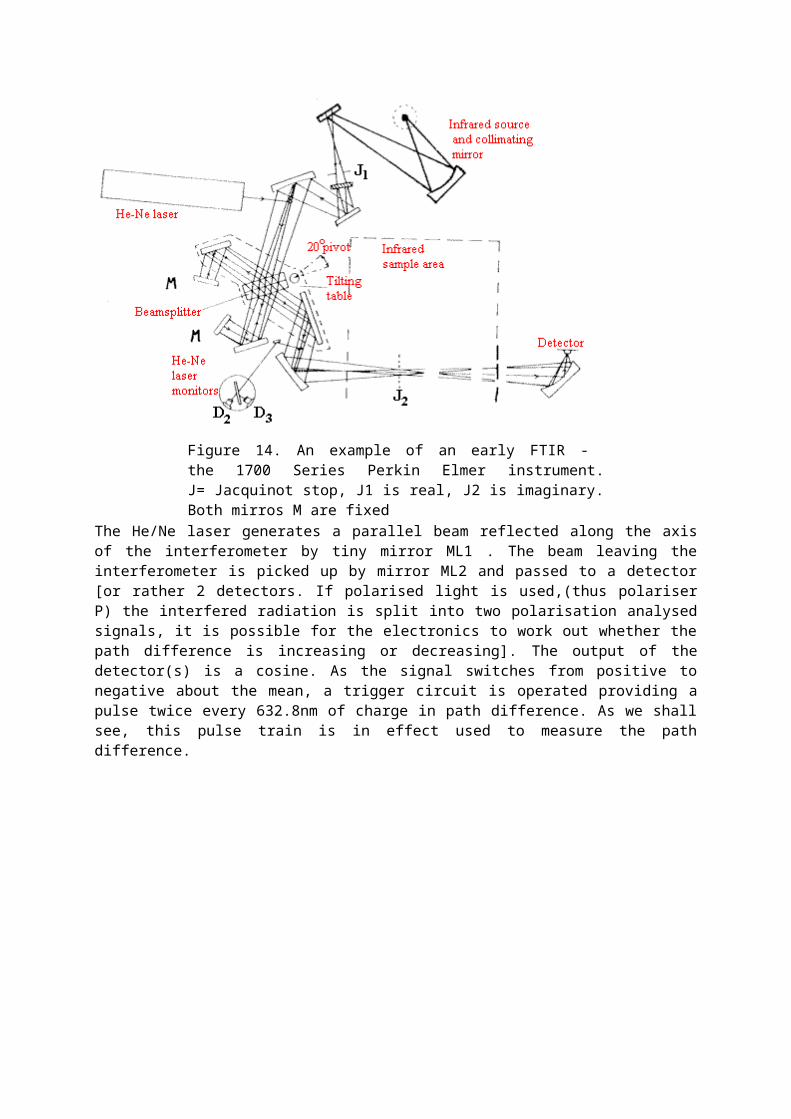
Figure 14. An example of an early FTIR - the 1700 Series Perkin Elmer instrument.

J= Jacquinot stop, J1 is real, J2 is imaginary.Both mirros M are fixed

The He/Ne laser generates a parallel beam reflected along the axis of the interferometer by tiny mirror ML1 . The beam leaving the interferometer is picked up by mirror ML2 and passed to a detector [or rather 2 detectors. If polarised light is used,(thus polariser P) the interfered radiation is split into two polarisation analysed signals, it is possible for the electronics to work out whether the path difference is increasing or decreasing]. The output of the detector(s) is a cosine. As the signal switches from positive to negative about the mean, a trigger circuit is operated providing a pulse twice every 632.8nm of charge in path difference. As we shall see, this pulse train is in effect used to measure the path difference.

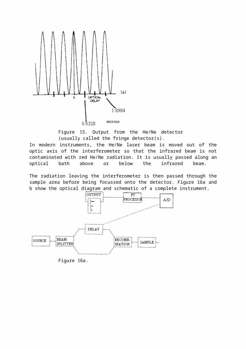
Figure 15. Output from the He/Ne detector (usually called the fringe detector(s).

In modern instruments, the He/Ne laser beam is moved out of the optic axis of the interferometer so that the infrared beam is not contaminated with red He/Ne radiation. It is usually passed along an optical bath above or below the infrared beam.

The radiation leaving the interferometer is then passed through the sample area before being focussed onto the detector. Figure 16a and b show the optical diagram and schematic of a complete instrument.

Figure 16a.

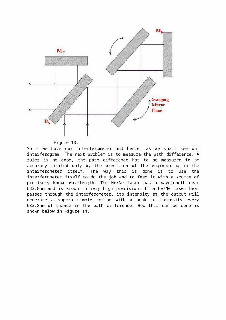
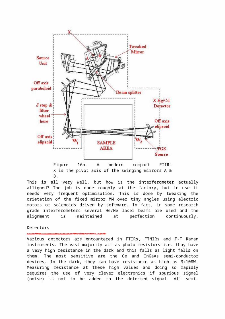
Figure 16b. A modern compact FTIR.X is the pivot axis of the swinging mirrors A & B.

This is all very well, but how is the interferometer actually alligned? The job is done roughly at the factory, but in use it needs very frequent optimisation. This is done by tweaking the orietation of the fixed mirror MM over tiny angles using electric motors or solenoids driven by software. In fact, in some research grade interferometers several He/Ne laser beams are used and the alignment is maintained at perfection continuously.

Detectors

Various detectors are encountered in FTIRs, FTNIRs and F-T Raman instruments. The vast majority act as photo resistors i.e. thay have a very high resistance in the dark and this falls as light falls on them. The most sensitive are the Ge and InGaAs semi-conductor devices. In the dark, they can have resistance as high as 3x108W. Measuring resistance at these high values and doing so rapidly requires the use of very clever electronics if spurious signal (noise) is not to be added to the detected signal. All semi-conductor detectors show an ‘absorption edge’ i.e. they will ignore radiation longer than a characteristic wavelength.Cooling detectors invariably reduces the amount of noise they develop [we are all familiar with noise. If you listen to your car radio you will be aware that in some areas the sound is clear, in others it is accompanied by hiss – this is "noise" in electronics language. The ratio of signal: noise (S:N) is critical in the measurement of electrical signals and also in the pleasure in listening to your car radio or mobile phone], but unfortunately cooling shifts the absorption edge towards shorter wavelength. Some detectors give adequate performance (an acceptable useful S:N ratio) at room temperature but others must be cooled. In an FTIR, one normally finds a TGS or similar detector for ordinary use. If better results [or more often, you need results on samples or sample accessories that transmit very little light] are required,

one then resorts to the use of a cryogenically cooled mercury cadmium telluride semi-conductor detector. Thus, these are invariably used in infrared microscopy and very often in diffuse reflection experiments.

The output from the detector goes to a preamplifier where it is converted into a voltage signal varying with time. This signal has to be digitised and the job is usually done with a dedicated 'analogue to digital' converter chip. These devices will measure the input voltage in binary numbers with 8, 16, 20 or 32 or more digits. Clearly, the number of useful digits is governed by the quality (S:N ratio) of the signal. 16 and 20 bit devices are frequently used.An A/D converter will carry out the conversion only when it is told to do so – it needs a pulse (or ‘handshake’) to tell it to do the job. The pulse is provided by the He/Ne fringe detector and trigger circuit. So, the A/D converter makes its measurement every 316.4nm of path difference. Clever, ain’t it? Thus, the He/Ne makes it possible to measure the interferogram at ultra precise path difference intervals. If the temperature changes, or you lean on the FTIR, the interferometer will very slightly distort and hence the interferogram will shift. However, the He/Ne beam will ALSO shift helping to correct for the distortion.The digitised interferogram is now fed to the F-T processor. This can be a dedicated chip or a PC. Obviously, a dedicated chip has its advantages (simplicity, lower cost etc) but the PC increases the versatility enormously. The block diagram looks like Figure 16b.Operation of FT instruments

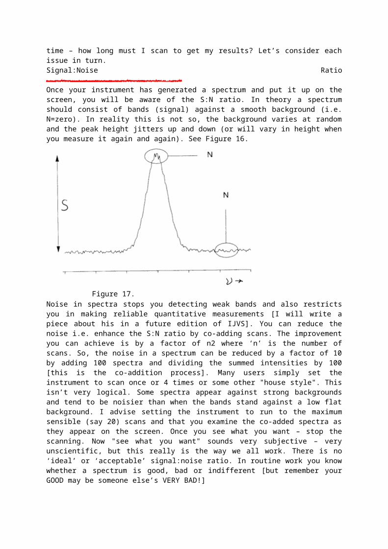
Spectroscopists are concerned predominantly about two parameters – signal:noise and resolution. To a lesser extent they worry about time – how long must I scan to get my results? Let’s consider each issue in turn.Signal:Noise Ratio

Once your instrument has generated a spectrum and put it up on the screen, you will be aware of the S:N ratio. In theory a spectrum should consist of bands (signal) against a smooth background (i.e. N=zero). In reality this is not so, the background varies at random and the peak height jitters up and down (or will vary in height when you measure it again and again). See Figure 16.

Figure 17. Noise in spectra stops you detecting weak bands and also restricts you in making reliable quantitative measurements [I will write a piece about his in a future edition of IJVS]. You can reduce the noise i.e. enhance the S:N ratio by co-adding scans. The improvement you can achieve is by a factor of n2 where ‘n’ is the number of scans. So, the noise in a spectrum can be reduced by a factor of 10 by adding 100 spectra and dividing the summed intensities by 100 [this is the co-addition process]. Many users simply set the instrument to scan once or 4 times or some other "house style". This isn’t very

logical. Some spectra appear against strong backgrounds and tend to be noisier than when the bands stand against a low flat background. I advise setting the instrument to run to the maximum sensible (say 20) scans and that you examine the co-added spectra as they appear on the screen. Once you see what you want – stop the scanning. Now "see what you want" sounds very subjective – very unscientific, but this really is the way we all work. There is no ‘ideal’ or ‘acceptable’ signal:noise ratio. In routine work you know whether a spectrum is good, bad or indifferent [but remember your GOOD may be someone else’s VERY BAD!]Recording spectra

When you record a spectrum you are, in fact recording two and ratioing them. Let me explain. You empty the sample area (or accessory) and record a BACKGROUND – you then insert the sample, run again and the computer produces a spectrum. What actually happens is that you first record the emission spectrum of source attenuated by the losses in the instrument, the response characteristics of the detector and any absorption along the optical path. The resultant BACKGROUND looks very different from the true emission characteristics of the source. Thus, the beam splitter characteristics and the performance of the detector attenuate the high frequency end of the spectrum. Meanwhile, H2O+CO2 in the optical path between the source and the detector cause sharp absorptions [Run the ‘BACKGROUND’ on your instrument and display it on the screen. You will see intense absorption around 2300cm-1 and 670cm-1 – these are due to CO2. The forest of bands around 3200 and 1600cm-1 are due to the vibration rotation spectrum of water – for an explanation refer to my piece in Edition 3, Volume 5 earlier this year].The next spectrum you then record is with the sample in place and again is the emission spectrum of the source, attenuated as before but ALSO by the sample. Usually this is not displayed but rather the second spectrum is immediately ratioed against the first on a point-by-point basis. The result is to show the difference between the two i.e. the spectrum of the sample which is what you want.Once you understand what happens several sources of possible error become clear –You can’t get meaningful results if you ratio nothing against nothing! So, if the background emission is non-existent, as it is over the CO2 absorption near 2300cm-1, you get no useful results.If you record the background under one set of conditions (resolution, number of scans etc) and the spectrum under another, the ratioing will be meaningless. It turns out that if the number of scans in the BACKGROUND is greater than that in the sample spectrum you are OK. You can, however, change the conditions between BACKGROUND and sample spectrum unwittingly.If you breath into the sample area as you insert the sample you will increase the CO2 and water vapour in the optical path. As a result, the BACKGROUND you are using is not appropriate and spurious bands will appear in your spectrum. If your instrument is purged with dry nitrogen, opening the sample area will introduce CO2 + H2O so the BACKGROUND and sample spectrum must again contain unwanted differences. This article is getting a little long so let me come back to these matters in another piece in a future edition.Resolution

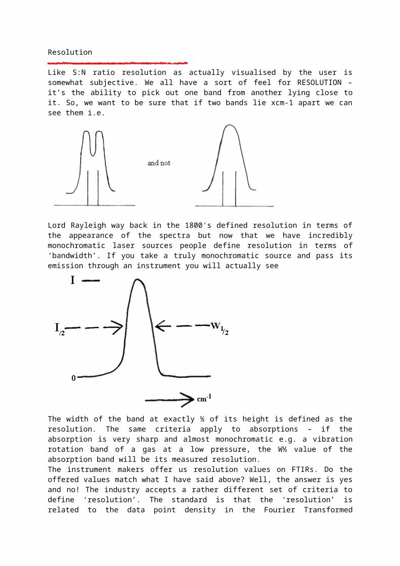
Like S:N ratio resolution as actually visualised by the user is somewhat subjective. We all have a sort of feel for RESOLUTION – it’s the ability to pick out one band from another lying close to it. So, we want to be sure that if two bands lie xcm-1 apart we can see them i.e.

Lord Rayleigh way back in the 1800's defined resolution in terms of the appearance of the spectra but now that we have incredibly monochromatic laser sources people define resolution in terms of ‘bandwidth’. If you take a truly monochromatic source and pass its emission through an instrument you will actually see

The width of the band at exactly ½ of its height is defined as the resolution. The same criteria apply to absorptions – if the absorption is very sharp and almost monochromatic e.g. a vibration rotation band of a gas at a low pressure, the W½ value of the absorption band will be its measured resolution.The instrument makers offer us resolution values on FTIRs. Do the offered values match what I have said above? Well, the answer is yes and no! The industry accepts a rather different set of criteria to define ‘resolution’. The standard is that the ‘resolution’ is related to the data point density in the Fourier Transformed Spectrum, the standard being that the resolution is ½ the data point density. Let me give you an example -–if you set the resolution at 2cm-1, the instrument will compute a spectral data point every wavenumber 4000, 3999, 3998………401, 400cm-1.The data points will then be joined up and that’s what you get. The quality of spectrum you actually see depends on the wavenumbers where the data points are calculated and the wavenumber of the emission or absorption bands but the industry standard is reasonable.So, I hear some of you ask – what resolution should I use? This is a very tricky question to answer: if the absorption band is very sharp – its W½ is small, you must use better resolution than if it is broad. The general rule is that to avoid missing the details in your spectrum, the resolution value MUST be less than the minimum W½ value of any bands in your spectrum. In the IR this is a pretty easy criterion to meet because the vast majority of bands are broad (W½ values >5cm-1and sometimes a lot wider than 10cm-1). In gas phase work, the bands can be incredibly narrow (low- pressure spectra can show W½ values as low as 0.1cm-1 routinely). Crystalline materials can sometimes catch you out and have relatively narrow lines but for most purposes 4cm-1 resolution is OK for analytical work. If the 4cm-1 spectrum looks as if it has fine detail in it – run a 2cm-1 spectrum [remember you must use a

new 2cm-1 BACKGROUND!] and see if there is any difference. If not, you can use 4cm-1 resolution in future.One obvious question is – why not record all spectra at the best resolution of which my equipment is capable? The answer is time (or more strictly S:N ratio).Remember, the resolution is standardised as a half of the data point density – so the number of data points between 4400 and 400cm-1 will be a modest 2000 at 4cm-1 resolution, but will rise to 16,000 at 0.5cm-1 resolution. To be able to calculate more data points, more points must be measured i.e. the inerferogram must be longer. In fact, the way it works out, the length of the interferogram – the distance scanned by the moving mirror equals 1/resolution. So – a machine capable of 0.1cm-1 resolution requires that MM will move by at least 10cm, a long way remembering the precision of movement required. This is why small cheap machine tend to offer only restricted resolution.Recording more data points is all very well, but more time is then needed to calculate the points in the spectrum. To sum up – using a better resolution than is required is simply not worth it because it loses time.There is also another variable. As resolution is improved and hence the mirror travel increases it becomes essential to restrict the beams that lie off the optical axis of the interferometer. To achieve this – the size of the Jacquinot Stop [JS in Figure 9 and 16b] is reduced as the resolution is improved. Typical values are ~8mm diameter at 4cm-1 resolution and perhaps 3mm at 1cm-1 or less. The effect is that less energy passes through the interferometer when operated at high resolution than at low. To the user this means that more scans are required to achieve an adequate S:N ratio – again soaking up even more time.To conclude, I have explained the basics of how your FTIR, FTNIR or FT-Raman works but I have said almost nothing about the ruses that you can adopt to fit the experiment to your needs. All instrument makers provide a wide range of software with their most basic instruments, but very few users actually try anything but the most bog standard set-up. This really is a pity.In the next volume, I will write a piece for you taking you through these features of your instrument showing you what you can do with them.REF: P.J.Hendra, Int.J.Vibr.Spec., [www.ijvs.com] 5, 5, 2 (2001)

3. Some Reminiscences from an Industrial SpectroscopistBill MaddamsI became an industrial Spectroscopist by chance; or perhaps my fairy godmother decreed it, as I had an interesting and challenging career spanning forty years and could not have wished for more. At the time that I was ready to enter university, in the autumn of 1943, deferment from military service was granted only for the study of a limited number of subjects and my ambitions to pursue chemistry came to an abrupt halt. I found myself at Sheffield University on a course called Radiophysics – whose purpose, ostensibly, was to provide radar technicians. However, at that stage of World War II it was assumed, correctly, that after graduation our services in this capacity would not be required, so, in practice, I took physics as the major subject together with subsidiary electronics and mathematics. We worked four terms per year and the normally three-year course was completed in two years and three months. Hence I graduated in December 1945 at the age of nineteen.At that stage I had no firm idea about my future; indeed, options were rather limited in the immediate post war era. In February 1946 I obtained the post of spectroscopist, working on ultra violet absorption spectroscopy, at Manchester Oil Refinery, a small concern on the western edge of the Trafford Park Industrial Estate. Although I was involved to a degree with petroleum products much of the work related to a subsidiary organisation, PetroCarbon Ltd, which had developed a cracking process that, produced mainly aromatic compounds. I worked on the quantitative analysis of mixtures of the three xylene isomers and ethylbenzene, which proved to be very good training for what I did later with infrared spectroscopy. I was also involved with the spectra of polycyclic aromatic hydrocarbons, many of which shared excellent vibrational fine structure, thus broadening my horizons.These measurements were made with a Hilger medium quartz spectrograph and a Spekker photometer. The modus operandi of the simple double beam system was to record a series of spectra over a range of absorbance values, using a variable aperture in the reference beam, on a photographic plate. This

took about twenty minutes and the plate was then developed. When dry, it was examined visually to determine the wavelength at which the intensity was equal in the beam passing through the absorbing compound and the attenuated reference beam. The usual practice was to work in absorbance increments of 0.05 up to about 1.2 and the total time required to measure a spectrum was about an hour.

The Spekker photometer is the accessory between the Source SC and the slit SL. Radiation from the electric arc between two iron electrodes illuminates lens L1 producing parallel light, which passes through two quartz cuvettes CS (sample) and CR (reference). Transmitted radiation is collected by lenses L2 and passed to the mirror prism assembly Mass. Radiation from the sample cuvette illuminates the top half of slit SL of the Hilger Medium Quartz Spectrograph. Radiation from CR

Bottom half of slit A is the aperture referred to in the script.

Hilger Medium Spectrograph capable of photographically displaying the line spectra of a source from the red to the UV (around 620 200nm). Range limited by the optical materials and the photographic plate sensitivity.Light from the slit SL is collimated by lens L3 passed through prism P and re-focussed by lens L4 [old-fashioned lenses and prism are made of quartz]. The prism has dispersion maximised in the UV hence the line spectrum at the glass photographic plate PH spreads as indicated. The plate gives only a black and white image of the line spectrum.

Each spectrum is represented as the Top and Bottom

half of the split - Source attenuated by Sample                         Source attenuated mechanically

Top Spectrum = Sample/Reference, 2nd Spectrum Sample/Attenuated reference etc.The poor spectroscopist looks for a match of the top and bottom spectra visually and then plots the points vs wavelength. Just to add to the little problems, the wavelength scale is incredibly non linear.

Between 1946 and 1951, I measured about three thousand spectra but felt increasingly, the need to broaden my horizons. Hence, in May 1951 I moved to the Research Department of The Distillers Co., situated in an exceedingly pleasant spot on the edge of Epsom Downs. I had been engaged to work on infrared spectroscopy in an already well-established laboratory headed by Tony Philpotts. However, as the result of staff changes I found myself involved in the determination of purities of 99+% hydrocarbons, studies used for detailed investigations on their oxidation rates. This was done via the measurement of their freezing curves, using a thermistor as thermometer coupled to a recording Wheatstone bridge. This posed a number of problems and I was able to draw on my physics background. I also continued with some ultraviolet absorption spectroscopy using a manual instrument, and electronic determination of intensity and point by point readings but, at least, it was a step forward from photographic plates!During this time I was rubbing shoulders with the infrared spectroscopists and learned a good deal before I became a fully-fledged member of the brotherhood. This was around the time that the first edition of Lionel Bellamy’s celebrated text on the interpretation of infrared spectra appeared and I absorbed its wisdom eagerly. Our workhorse spectrometer was a Perkin Elmer 12C single beam instrument, which although producing spectra on a chart recorder, had a considerable manual component in its operation. In order to compensate for the pseudo black-body intensity output of the source as a function wavelength, the slit width was adjusted manually, in a series of steps. Thus, commencing scanning at 15µ with a wide slit the spectrum was run as far as 14 µ, whereupon the slit width was reduced somewhat and the process was continued sequentially to the short wavelength limit. The total time required to run a spectrum was about twenty minutes.At that time we used infrared spectroscopy extensively for the quantitative analysis of the oxidation products of cumene (isopropyl benzene) to its hydroperoxide, which was then cleaned with diluted acid to give phenol and acetone. In the oxidation process two undesirable by-products, acetophenone and phenyl dimethyl carbinol were formed and, predictably much work was done to find conditions that minimised their concentration. It proved possible to measure them at quite low levels. In the case of acetophenone (phenyl methyl ketone), the u (C=O) band was used despite interference from water vapour bands appearing in that wavelength regions because of the single beam mode of operation of the instrument. We became very proficient at the visual substraction of this interference! Analyses of mixtures of three or four components, none of them minor, were done as necessary.The first approach with such analyses was to set up calibration curves of absorbance as a function of concentration for each component. These sufficed if not too high a degree of precision was required. For greater accuracy matching mixtures of pure components were prepared, using micro-pipettes, whose composition approximated to the values obtained from the calibration curves. Measurements on these mixtures were then used to analyse the unknown. Although this approach was somewhat time consuming it was often possible to obtain a precision of 1% or 2% with three of four component mixtures.A few months after I joined the team, Ray Ward arrived on the scene and his major occupation for some time was the construction of a double beam spectrometer with a photometric system. This was based on a Grubb Parsons optical unit and the challenge lay in devising a photometric system, driven by the off-balance signal between the two beams. The attenuater in the reference beam was constructed from a semi-circular metal strip into which teeth were cut so that, as it rotated, increasing attenuation was obtained. The system involved a series of pulleys beneath the optical unit and these were inter-connected by wire. The system worked well until the wire wore and broke, which happened rather too frequently for those of us who then had to tip the unit on its side and replace the wire. Surprisingly, perhaps, this in no way disturbed the optics. This spectrometer was in use for a long period of time and proved very effective.

The next addition to our armoury was a Unicam SP100 spectrometer which, by comparison, was an all singing all dancing act, with considerable flexibility in its operating conditions. Retrospectively, it was ahead of its time in at least two respects. Firstly, the analytical problems we encountered usually did not require this wide degree of flexibility. For example, we seldom needed to run high resolution vapour phase spectra. Secondly, the concepts involved in its construction were very sound, but this could not be said of all the components involved. Two problems come to mind.It used a Golay pneumatic detector, which provided good sensitivity, but failed more frequently than we would have wished. Their replacement was rather complicated because of the construction of the optical unit. This was designed to be operated under vacuum or filled with dry air/nitrogen, and a heavy lid covering the whole unit needed to be removed. When it was replaced there was often a problem in making it airtight, as the ‘O’-ring seal did not bed down easily. By trial and error we concluded that the optimum method was to sit a young lady assistant on top of the case , turn on the vacuum pump and wait until the reduction of pressure inside provided the necessary force to ensure a good seal!These was an appreciable amount of synthetic organic chemistry in progress, and this often produced some challenging qualitative analysis when all did not go to plan so far as the chemistry was concerned. I particularly enjoyed this type of work as it gave me the opportunity to go back to my first love, chemistry. I would try to deduce what alternative reaction might have occurred and attempt spectral interpretations on that basis. We always had excellent working relations with all of those who submitted samples and they often provided background information that was of considerable assistance. By that time gas chromatography was making an impact and trapped out GC fractions of unknowns appeared with increasing regularity. As a consequence micro infrared cells became part of our everyday routine.In 1959 I became Section Head, Spectroscopy. The paperwork involved did not prove too much of a burden and I was still an active infrared spectroscopist. However, the scope of the Section gradually enlarged to encompass first mass spectroscopy, then x-ray fluorescence spectroscopy, plus some x-ray diffraction and finally NMR spectroscopy. Inevitably, to a degree I then became a jack of all trades, but infrared spectroscopy was not wholly a thing of the past, particularly as I became more involved with polymer characteristics.At that time Distillers Chemicals & Plastics was well established in the PVC business and then became a licensee of the Philyro process for the manufacture of high density (linear) polyethylene. So far as this latter is concerned, the technical know-how also included an infrared method for measuring the low level of chain branching, which was rather involved and required absorbance measurements at accurately defined wave numbers. The SP100 instrument was ideal for this purpose, but not for the more direct method using a wedge of polymethylene in the reference beam. This was adjusted to eliminate the peak characteristic for methylene groups upon which the much weaker peak specific for the methyl groups of the chain branches is superimposed. The Grubb Parsons instrument proved ideal, because of the easy access to the sample compartment, which facilitated manual adjustment of the wedge. The method was automated at a later date using a Perkin-Elmer 577 spectrometer fitted with a punched tape output to record the spectral data for both sample and a polymethylene film and the subtraction process was then done on a computer.Although PVC has been widely used for many years for a range of commercial purposes it has its limitations. Foremost among these is the way in which it darkens in use, due to the sequential elimination of HCl units, leading to the formation of conjugated polyene units, which absorb in the visible spectral region. This led to the use of a variety of stabilisers incorporated into the polymer. It had been recognised empirically that materials prepared at lower than normal polymerisation temperatures were less prone to the decomposition but, unfortunately, were too rigid and brittle for many purposes. However, the effect of polymerisation temperature on both photo and thermal degradation, a problem in sample processing when stability is required, suggested that the problem had its origin in defect structures along the chain, either rogue chemical structural units and/or faults in the conformational and configurational irregularity.Hence, I found myself investigating this latter problem, which proved challenging but fascinating and I can only touch upon these. Quite fortuitously, the u(C-Cl) modes between about 600 and 700cm-1are sensitive to both the conformational and configurational structures as had already been demonstrated by Professor Krimm and workers at B.F.Goodrich. My interest lay in deciding how much quantitative

information could be obtained by this approach. The inherent problem is that the various peaks in the u (C-Cl) region overlaps to varying degrees. Hence, I turned initially to the use of a Du Pont curve resolver, which is useful but has its limitations, not least because it does not provide a 'goodness of fit' criterion. It was also necessary to assume that the peaks are Lorentzian in shape and this, in turn, led me to measure peak shapes for a variety of simple molecules and, where deviations from the Lorentzian form occurred, find simple mathematical equations to represent them. The work was done on the PE577 spectrometer coupled to a punched tape output system, mentioned earlier.Quite fortuitously, these studies began after The Distillers Co., sold its chemical and plastics interests to BP in 1967 and we became an out station of the main BP Research Centre at Sunbury on Thames. Although I then found myself burdened with additional paperwork, the new management system had one major advantage. Whereas the development with Distillers was done when there was any spare time, the BP system required us to devote a fixed proportion of our time to it, having first obtained approval for lines of work deemed to be of long term value. The PVC study came into this category.Nevertheless, I realised that it required appreciably more effort than I was able to devote to it from the manpower available to me. I was fortunate in being able to pursue the matter via BP sponsored C.A.S.E. awards, with David Bower in the Physics Department at Leeds University and with Bill George, initially at Kingston Polytechnic and subsequently The Polytechnic of Wales. The Leeds work was an amalgam of our respective interests. My aim was to pursue the computer curve fitting of the PVC spectrum in greater depth and David Bower was interested in measuring molecular orientation in chain PVC specimens using Raman spectroscopy. This required a reliable quantitative separation of the overlapping peaks and, in the event, the PhD student spent three years on the problem, and obtained a great deal of useful information, both on computer curve fitting and the relative concentrations of the conformational and configurational isomers of PVC. A second student was then able to make some very useful orientation measurements.The work done by Bill George and his students also related to these isomers, but in a different way. His interest was in making variable temperature infrared measurements to determine the energy difference between conformational isomers. He worked initially on a series of carbonyl-containing compounds and then moved to low molecular weight models for PVC, namely meso- and dl-2, 4-dichloropentone and the three configurational isomers of 2, 4, 6-tricholorheptane. Most of the work was done in solution, but some measurements were made by the matrix isolation technique, as a means for peak sharpening.By the early 1970’s we were examining a wide range of compounds by infrared spectroscopy and were encountering an increasing number of materials, mostly solids, from which it was difficult to obtain spectra. The A.T.R technique was not always the answer. Hence, I became interested in the scope of Raman spectroscopy for dealing with such materials. Bill George, then at Kingston Polytechnic, had a JEOL Raman spectrometer and as it was not far distant from our Epsom site, Don Gerrard made occasional trips there to run exploratory spectra, which by and large, proved useful.Around this time I read an application reporting the Raman spectrum of a thermally degraded PVC sample in which conspicuous C=C peaks appeared, from the conjugated polyene sequences that were present. What the authors had not appreciated at the time was the temperature of degradation of their sample was such that the total level of polyenes could not have been more than about 0.01%. So that the intensity of the polyene peaks must have been very high and furthermore, the sensitivity of the method offered distinct analytical potential. The authors vaguely suggested that they were observing a resonance Raman spectrum, but did not pursue the matter. This was a challenge I could not resist.I was able to obtain PVC samples with known levels of degradation, measured via the HCl evolved, from a group working at the BP Chemicals Barry (South Wales) site, where the polymer was made and that provided the starting point for much work that proved to be both interesting and valuable. We were able to show that the spectra were indeed the result of resonance enhancement, from the presence of strong harmonic and combination peaks and other features. However, by far the most significant result was that u(C=C) varied with different exciting wavelengths, dropping in frequency as the wavelength of the exciting line increased. This is because we were exciting resonance in polyenes of different sequence lengths and u (C=C) decreases as the sequence length increases, thus providing a valuable diagnostic tool.Soon after this initial work, the Epsom laboratories were closed and we moved to Sunbury upon Thames. This move, although logical from the company viewpoint, was not without its disadvantages.

However, retrospectively, it became evident that these were strong compensating advantages. The foremost being that there was more money for equipment. Hence, it was not long before we had our own Raman spectrometer and the PVC degradation studies proceeded apace. By way of summary it suffices to say that the technique proved very valuable for assessing thermal and photodegradation and the influence of plasticisers and fillers.We also acquired our first FTIR spectrometer soon after the amalgamation of the two laboratories and this proved exceedingly useful for both day to day analytical work and for the PVC structural studies. So far as the latter were concerned I was able to pursue other methods for studying the overlapping peak problem. Among these was second and fourth derivative spectroscopy, which leads to peak sharpening but an increase in spectral noise. Hence good quality primary data were necessary and readily obtainable by repetitive scanning. I also assessed the potentialities of Fourier self-deconvolution for peak finding, rather than for quantitative work, where considerable problems exist.I must confess that I never ran an FTIR spectrum. During the years that preceded by retirement I was in charge of a group of about a dozen and a half people, also including specialists but administrative duties occupied a significant proportion of my time. However, I was fortunate in having capable and enthusiastic staff who would run spectra for me which, like as not, I often interpreted out of hours. I would then come back and ask for more! I progressed a long way from my initial infrared work on analysis of the oxidation products of cumene, but I always regarded myself as an applied spectroscopist. That said, I was fortunate enough to be working at a time when spectrometers and techniques advanced enormously, more or less at the same rate that increasingly challenging samples were thrust upon us. I was also fortunate in having worked with a number of spectroscopists whose interests were primarily academic, but appreciated that there is an appreciable overlap between pure and applied spectroscopy.I could not have terminated by spectroscopic interest abruptly when I left BP and happily did not do so. However, that is another story, which does not come within the context of the present reminiscences!

REF: B. Maddams, Int.J.Vibr.Spec., [www.ijvs.com] 5, 5, 3 (2001)