Embed Size (px)
Citation preview
Homotopy theory and classifying spaces
Bill Dwyer
Copenhagen (June, 2008)
Contents
1. Homotopy theories and model categories . . . . . . . . . . . . . . . . . . 3
What is a homotopy theoryT? – Examples of homotopy theories (Tpair presentation)– The homotopy categoryHo(T) – Examples of homotopy categories – Model cat-egory: (C, E) with extras – Examples of model categories(C, E) – Dividends froma model category structure on(C, E) – Equivalences between homotopy theories –T(C, E) ∼ T(C′, E ′) for model categories – Examples of equivalences between ho-motopy theories
2. Homotopy limits and colimits . . . . . . . . . . . . . . . . . . . . . . . . 17
Colimits and related constructions – Aside: notation for special coends – Homo-topy colimits and related constructions – Model category dividend – Constructionof hocolim, version I – Construction ofhocolim, version II – Homotopy limits andrelated constructions – Another model category dividend – Construction ofholim,version I – Construction ofholim, Version II – Properties of homotopy (co)limits –Mysteries of (I) and (II) revealed
3. Spaces from categories . . . . . . . . . . . . . . . . . . . . . . . . . . . . 29
Categories vs. Spaces – The Grothendieck Construction – Thomason’s Theorem –Variations onCnF (all ∼ on N) – Extension to homotopy coends – The paralleluniverse ofHom and⊗ – Properties of Kan extensions – Does pulling back preservehocolim? – Terminal functors – Does pulling back preserveholim? – Initial functors
4. Homology decompositions . . . . . . . . . . . . . . . . . . . . . . . . . . 40
Approximation data forBG – Approximation data fromG-orbits – Obtaining alterna-tive approximation data – SixZ/p-homology decompositions – How to obtain the sixdecompositions – Identify hocolim for subgroup diagram – Identify hocolim for cen-tralizer diagram – Relate posets KC2 ∼ KC1 – Relate posets KC3 ∼ KC2
1
2
5. Localizations . . . . . . . . . . . . . . . . . . . . . . . . . . . . . . . . . 46
Left Bousfield localization – Example with discrete categories – Another model cat-egory dividend – Examples of model category localizations (I) – Examples of modelcategory localizations (II) – Localization with respect toR-homology,R ⊂ Q –Localization with respect toZ/p-homology – MixingLQ(X) with the Lp(X)’s torecoverX – An approximation toLp – The Bousfield-Kanp-completionCp – TheBousfield-Kanp-completionCp: good & bad
6. Cohomology of function spaces . . . . . . . . . . . . . . . . . . . . . . . 56
The Steenrod algebraAp – Modules and algebras overAp – The functorT – ThefunctorT ↔ function spaces out ofBV – Lannes works his magic – Outlining theproof – The caseX = K = K(Z/p, n) – The case in whichX is p-finite. – TowerUs = · · · → Un → Un−1 → · · · → U0 – T and maps fromBV – In thepresence of a volunteer. . .
7. Maps between classifying spaces . . . . . . . . . . . . . . . . . . . . . . 68
Cohomology of homotopy fixed point sets –X a finite complex: setting the scene –X a finite complex (II) – Aside: sighting ofCp(p-bad space) – MapsBQ → BG:individual components – MapsBQ → BG: how many components? – Maps intoCpBG for G finite – Fusion functors – Fusion systems
8. Linking systems andp-local classifying spaces . . . . . . . . . . . . . . . 78
DoesF determineCpBG? – Switch to thep-centric collection – Thep-centric cen-tralizer diagram – The categoricalp-centric centralizer model – The linking system –Lc vs.Fc – the orbit picture – Lifting fromHo(Sp) to Sp – Fusion relations suffice!– p-local finite groupX
9. p-compact groups . . . . . . . . . . . . . . . . . . . . . . . . . . . . . . . 89
Definition of ap-compact group – Some basic properties ofp-compact groups – Morecohomology of homotopy fixed point sets – The centralizer ofV in X is ap-compactgroup. – The centralizer ofV in X is a subgroup –∃ non-trivialV → X – Existenceof a Sylowp-subgroup for finiteG – Existence of a maximal torus inX
10. Wrapping up . . . . . . . . . . . . . . . . . . . . . . . . . . . . . . . . 99
Another commutative diagram? – Homotopy theories – Localizations & completions– The functorT andH∗ Homh(BV,−) – Homology decompositions and maps toBG – p-compact groups andp-local finite groups – Conclusion
Lecture 1: Homotopy theories and model categories 3
Lecture 1.
Homotopy theories and model categories
These arerough notes. Read at your own risk! The presentation is notnecessarily linear, complete, compact, locally connected, orthographically
defensible, grammatical, or, least of all, logically watertight. The author doesn’t alwaystell the whole truth, sometimes even on purpose.
This first lecture is deep background: before getting to classifying spaces, I’d like todescribe some homotopy theoretic machinery. The first question to ask before tryingto understand this machinery is averybasic one.
Slide 1-1 Slide 1-1
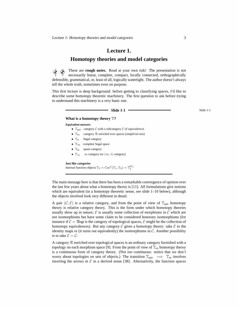
What is a homotopy theoryT?
Equivalent answers• Tpair categoryC with a subcategoryE of equivalences
• Ten categoryR enriched over spaces (simplicial sets)
• Tsc Segal category
• Tcss complete Segal space
• Tqc quasi-category
• T∞ ∞-category (or(∞, 1) category)
Just like categoriesInternal function objectsT3 = Cath(T1, T2) = ThT1
2
The main message here is that there has been a remarkable convergence of opinion overthe last few years about what a homotopy theory is [11]. All formulations give notionswhich are equivalent (in a homotopy theoretic sense, see slide 1–10 below), althoughthe objects involved look very different in detail.
A pair (C, E) is a relative category, and from the point of view ofTpair homotopytheory is relative category theory. This is the form under which homotopy theoriesusually show up in nature;E is usually some collection of morphisms inC which arenot isomorphisms but have some claim to be considered honorary isomorphisms (forinstance ifC = Top is the category of topological spaces,E might be the collection ofhomotopy equivalences). But any categoryC gives a homotopy theory: takeE to theidentity maps or (it turns out equivalently) the isomorphisms inC. Another possibilityis to takeE = C.
A categoryR enriched over topological spaces is an ordinary category furnished with atopology on each morphism space [9]. From the point of view ofTen homotopy theoryis a continuous form of category theory. (Nottoo continuous: notice that we don’tworry about topologies on sets of objects.) The transitionTpair =⇒ Ten involvesinverting the arrows inE in a derived sense [38]. Alternatively, the function spaces
Lecture 1: Homotopy theories and model categories 4
in the simplicial category can be view as spaces of zigzags in the original categoryC,where the backwards-point arrows lie inE [36].
A Segal category is a simplicial space which is discrete at level 0 and satisfiessome homotopical product conditions [89] [10]. The transitionTen =⇒ Tsc
amounts to taking the nerve, and treating it as a simplicial space.
A complete Segal space is simplicial space which is not necessarily discrete atlevel 0 and satisfies some homotopy fibre product conditions and some other
homotopical conditions [89] [11]. The transitionTsc =⇒ Tcss requires repackaginggroup-like topological monoids of equivalences into their associated classifying spaces,but leaving the non-invertible morphisms alone. This is an unusually transparent modelfor a homotopy theory: an equivalence is just a map between simplicial spaces whichis a weak equivalence at each level. Internal function objects are also easy to come byhere.
A quasi-category (∞-category) is a simplicial set, treated from what classicallywould be a very peculiar point of view [62] [63]. In some sense this is the most
economical model for a homotopy theory.
1.1 Exercise.Let C be a category andE its subcategory of isomorphisms.In this particular case, describe in detail each of the various models for the
homotopy theory ofT(C, E).
The notationCath(T1, T2) or ThT12 denotes the homotopy theory of functors from the
first homotopy theory to the second, but taken in the correct homotopy theoretic way.The notationThT1
2 is very similar to a notation for homotopy fixed point sets that willcome up later on (2.28), but I’ll use it anyway. This same ambiguity comes up withoutthe “h”: if X andY are spaces,Y X is the space of maps fromX to Y , but if Y is aspace andG is a groupY G is the fixed-point set of the action ofG onY .
The above internal function objects for homotopy theories are tricky to define correctlyin some models, but can have a very familiar feel to them. If(C, E) and(C′, E ′) are twocategory pairs in which all of the morphisms inE andE ′ are invertible, then the functionobjectCath(T(C, E), T(C′, E ′)) is equivalent in the sense of homotopy theories to thecategory in which the objects are functorsC → C′ and the morphisms are naturaltransformations. (To promote this to a homotopy theory, pick natural isomorphismsbetween functors as equivalences.)
? 1.2 Exercise.Let G andH be two discrete groups, treated as one-object categoriesor as homotopy theories (the latter by designating all morphisms as equivalences). De-scribe the groupoid of functorsG → H in terms of the group structures ofG andH.How many components are there to the groupoid? What are the vertex groups?
1.3 Exercise.Let C be a category, and letE = C. LetTop be the homotopy the-ory of topological spaces, where the equivalences are taken to be weak homotopy
equivalences. What geometric structures do you think are described by the homotopytheoryCath(T(C, E),Top)?
Lecture 1: Homotopy theories and model categories 5
Slide 1-2 Slide 1-2
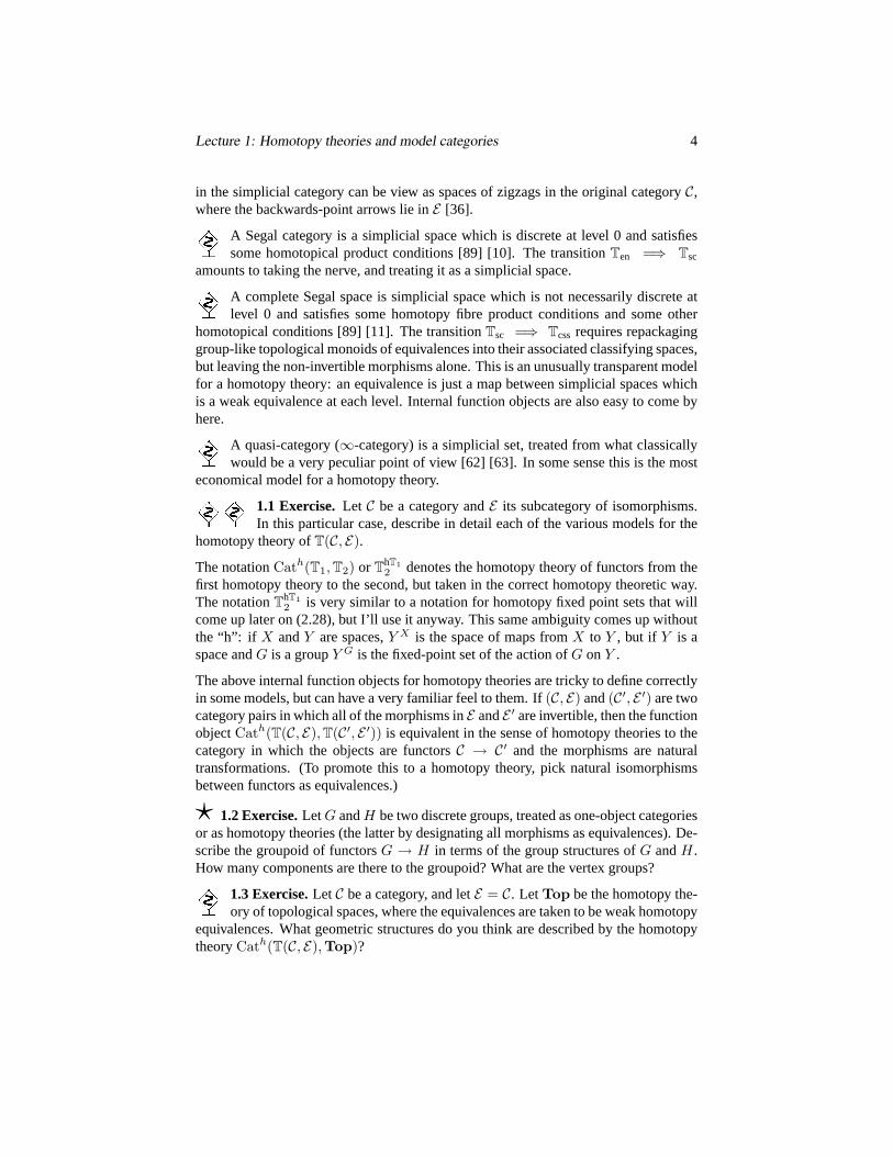
Examples of homotopy theories (Tpair presentation)
GeometryNotation C ETophe Top homotopy equivalencesTop Top weak homotopy equivalencesTopR Top R-homology isomorphismsTop≤n Top iso onπi for i ≤ n
AlgebraSp simplicial sets |f | an equivalence inTopsGrp simplicial groups |f | an equivalence inTop
simp. rings, Lie alg.,etc (same)ChR chain complexes overR homology isomorphisms
DG algebras homology isomorphisms
The first four examples illustrate the fact that a category can be associated with manydifferent homotopy theories. For instance, inTop≤n the(n + 1)-sphere is equivalentto a point, but itTop it isn’t.
1.4 Exercise.Give an example of a map which is an equivalence inTop but notin Tophe.
Simplicial sets. Simplicial sets [49] [70] are slightly more complicated analogs ofsimplicial complexes. They have two advantages over simplicial complexes:
• Better colimit properties. In a simplicial complexX a simplex is determined byits set of vertices, so collapsing the vertices ofX to a single point in the categoryof simplicial complexes causesX itself to collapse to a point. But it’s hard notto want to collapse the two endpoints of a one-simplex together to get a circle.Simplicial sets possess monolithic simplices of various dimensions; these havevertices but are not determined by them. Collapsing is easy.
• Better limit properties. The relationship between the geometric realization ofthe (categorical) product of two simplicial complexes and the product of theirrealizations is obscure. (At best these two spaces have the same homotopy type).There is no such problem with simplicial sets.
There is a short discussion of how to get from simplicial complexes to simplicial setsin [43, §3]. Simplicial complexes are based on the category∆, which can be describedup to isomorphism in (at least) the following three ways. (Note that any (partially)ordered set gives an associated category, in which there is a unique morphismx → yif x ≤ y.)
1. ∆ is the category whose objects are the ordered setsn = 0, . . . , n, n ≥0, and whose maps are the weakly order-preserving maps between these sets(“weakly”= preserves≤).
Lecture 1: Homotopy theories and model categories 6
2. ∆ is the category whose objects are the finite ordered simplicial complexes∆n,n ≥ 0 and whose maps are the simplicial complex maps between these objectswhich are weakly order-preserving on the vertices. (Here∆n is the space ofconvex linear combinations of0, . . . , n.)
3. ∆ is the category whose objects are the finite categoriesn, n ≥ 0, and whosemorphisms are the functors between them.
A simplicial setX is a contravariant functor from∆ to Set, i.e., a functorX : ∆op→Set; maps between simplicial sets are natural transformations of functors. For eachn ≥ 0, X has a setXn = X(n) = X(∆n) of n-simplices, and these sets are related byvarious face maps, degeneracy maps, and their composites. For example, there are twoface (vertex) mapsX1 → X0, corresponding to the two vertex inclusions∆0 → ∆1,and one degeneracy mapX0 → X1 corresponding to the collapse∆1 → ∆0.
1.5 Exercise.Any topological spaceY has an associated simplicial setSing(Y ), thesingular complex ofY , given bySing(Y )n = Hom(∆n, Y ). Given this and the usualconstruction of singular homology, how would you define the homology of a simplicialset?
The geometric realization functor for simplicial complexes extends to a geometric re-alization functor|(−)| for simplicial sets; the realization functor is left adjoint to thesingular complex functor (1.5). The realization ofX can be obtained explicitly as|X| = X×∆∆∗; the notation stands for the cartesian product over∆ of the contravari-ant functorX with the covariant functor∆∗ (slide 2–2). Both of these are functors toTop, where we think ofX as taking values in discrete spaces. More formally,|X| isthe coend of the functor(n,m) 7→ Xn ×∆m on∆op×∆.
1.6 Exercise.Draw an analogy betweenF×CG, for (F : Cop→ Top, G : C → Top),andM ⊗R N , for (M a rightR-module,N a leftR-module). Check the formula
M ⊗R N ∼= R⊗Rop⊗ZR (M ⊗Z N)
(which seems to relate⊗R to Hochschild homology). What’s the corresponding for-mula if any forF ×C G?
? 1.7 Exercise.Observe that any categoryC has an associated simplicial setN(C),the nerve ofC, with N(C)n = Hom(n, C) (hereHom denotes the set of functors).Try to determine the homotopy type of|N(C)| in some simple cases, e.g., ifC is thepushout category (three objectsa, b, c, and mapsb → a andb → c), or if C is the(co-)equalizer category (two objectsa, b, and two distinct mapsa→ b).
? 1.8 Exercise.Let I be the category0→ 1 (i.e., the categoryn for n = 1). Verifythat N(I) is the simplicial set which corresponds to the ordered simplicial complex0, 1, 0, 1; its geometric realization is the interval. Observe that a functorF :C → D gives a mapN(C)→ N(D) of simplicial sets, and that a natural transformationbetweenF,G : C → D gives a homotopyN(C × I) ∼= N(C)×N(I)→ D.
? 1.9 Exercise. Conclude that if a categoryC has a terminal object or an initialobject, thenN(C) has a contractible geometric realization.
Lecture 1: Homotopy theories and model categories 7
1.10 Exercise. Convince yourself that ifK is a finite simplicial complex andC isthe category determined by the poset of simplices ofK (ordered by inclusion), then|N(C)| is homeomorphic to|K|. Conclude that any finite complex is weakly homotopyequivalent to the nerve of a category. What about any topological spaceX? Can youchoose the category and the weak equivalence to be natural inX?
1.11 Exercise.If K is a simplicial complex, there is a simplicial setSing(K) givenby letting Sing(K)n be the set of simplicial complex maps∆n → K (these mapsare not required to be monomorphisms on the vertex sets). Check that|Sing(K)| isnot necessarily homeomorphic to|K|. Are they homotopy equivalent? Check that thesituation is substantially nicer ifK is an ordered simplicial complex andSing(K) isdefined in terms of (weakly) ordered simplicial set maps∆∗ → K.
1.12 Exercise.The process of passing from (ordered) simplicial complexesto simplicial sets is not totally unrelated to the passage from varieties over a
field to objects inA1-homotopy theory. A simplicial set is a contravariant functor fromfinite ordered simplicial complexes to sets which takes whatever pushouts exist in thedomain category to pullbacks in the range. The first step in constructingA1-homotopytheory is to consider contravariant functors from varieties to simplicial sets which takecertain pushout-like diagrams in the category of varieties to homotopy pullbacks ofsimplicial sets. Are there any other examples of this kind of construction?
Simplicial objects. A simplicial object in a categoryC is a functor∆op→ C.
1.13 Exercise. Let R be a ring and consider an object in the categorysModR ofR-modules. There is a normalization functorN : sModR → ChR, which involvesdividing out by images of degeneracy maps and taking the alternating sum of the facemaps. The functorN establishes an equivalence of categories betweensModR andthe category of non-negatively graded objects ofChR. Familiarize yourself with this[70, Chap. 5] [49, III.2]. What isN−1(R[n]), whereR[n] is the chain complex whichis zero except for a copy ofR in degreen?
Non-abelian homological algebra. Simplicial objects can serve as substitutes forchain complexes in categories which are not abelian. For instance, Quillen [84] definedcohomology for a commutative ringR by applying an “indecomposables” functor to asimplicial resolution ofR, in much the same way as you might define higher Tor’s foranR-module by applying a tensor product functor to a chain complex resolution of themodule.

Lecture 1: Homotopy theories and model categories 8
Slide 1-3 Slide 1-3
The homotopy categoryHo(T)The most visible invariant of a homotopy theoryTpair Ho(C, E) = E−1CTen Ho(R) = π0R (i.e. π0(morphism spaces))
Pluses and minuses
• Elegant (but only a small part of the structure)
• Can be hard to compute in theTpair case.
FormingHo(C, E) involves taking seriously the idea that the maps inE are honoraryisomorphisms:Ho(C) is the category which results if the morphisms inE are forciblydeclared to be isomorphisms.
1.14 Exercise.Let K be a finite simplicial complex,C the poset of simplices ofK(ordered by inclusion) andE = C. The categoryHo(C) is a groupoid (because everymorphism has been made invertible). Can you identify this groupoid in some simplecases? In general?
1.15 Exercise. In the above situation, can you guess what the categoryR en-riched over spaces which corresponds toT(C, E) looks like? What is lost in this
case in passing fromT(C, E) to Ho(T(C, E))? Is it always the case that something islost?
Slide 1-4 Slide 1-4
Examples of homotopy categories
Geometry(C,E) MapsX → Y in Ho(C, E)Tophe homotopy classesX → YTop homotopy classesCW(X)→ YTopR homotopy classesCW(X)→ LR(Y )Top≤n homotopy classesCW(X)→ Pn(Y )
AlgebraSp homotopy classes|X| → |Y |sGrp pointed homotopy classesB|X| → B|Y |ChR chain homotopy classes Proj. Res.(X)→ Y
Note:CW(X) denotes a cell complex which is weakly equivalent to the spaceX.
There is a general theme in the above examples: mapsX → Y in the homotopycategory of(C, E) are computed by finding some kind of a nice stand-inX ′ for X andcomputing some sort of equivalence classes of maps inC from X to Y . Clearly, thereis extra structure in the categories which makes this possible.
Lecture 1: Homotopy theories and model categories 9
1.16 Exercise.Try to make one of the above calculations by hand, for instance, in theTop case. First, construct a categoryQ in which the objects are spaces and the mapsX → Y are given by[CW(X), Y ]. (Observe that[CW(X), Y ] ∼= [CW(X),CW(Y )]).Then build a functorTop→ Q. Show that the functor sends weak equivalences to iso-morphisms and that it is universal with respect to this property.
One of the most convenient frameworks in which it is possible to make calculationslike this is the framework of Quillen model categories.
Slide 1-5 Slide 1-5
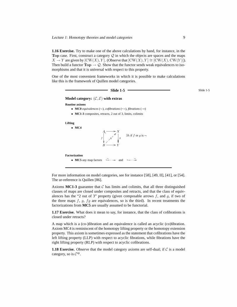
Model category: (C, E) with extras
Routine axioms• MC0 equivalences(∼), cofibrations(→), fibrations()
• MC1-3 composites, retracts, 2 out of 3, limits, colimits
Lifting
• MC4A _
f
// X
g
B //
h~~
>>~~
Y
∃h if f or g is∼
Factorization
• MC5 any map factors∼→ · and → · ∼
For more information on model categories, see for instance [58], [49, II], [41], or [54].The ur-reference is Quillen [86].
Axioms MC1-3 guarantee thatC has limits and colimits, that all three distinguishedclasses of maps are closed under composites and retracts, and that the class of equiv-alences has the “2 out of 3” property (given composable arrowsf , andg, if two ofthe three mapsf , g, fg are equivalences, so is the third). In recent treatments thefactorizations fromMC5 are usually assumed to be functorial.
1.17 Exercise.What does it mean to say, for instance, that the class of cofibrations isclosed under retracts?
A map which is a (co-)fibration and an equivalence is called an acyclic (co)fibration.Axiom MC4 is reminiscent of the homotopy lifting property or the homotopy extensionproperty. This axiom is sometimes expressed as the statement that cofibrations have theleft lifting property (LLP) with respect to acyclic fibrations, while fibrations have theright lifting property (RLP) with respect to acyclic cofibrations.
1.18 Exercise.Observe that the model category axioms are self-dual; ifC is a modelcategory, so isCop.
Lecture 1: Homotopy theories and model categories 10
1.19 Exercise.UseMC4 in combination with the retract property to show that in amodel categoryC a mapf is a cofibration if and only iff has the LLP with respect toacyclic fibrations, or an acyclic cofibration if and only if it has the LLP with respectto fibrations. (By duality, there are parallel characterizations of fibrations and acyclicfibrations.) Conclude that, given the equivalences, the fibrations and cofibrations de-termine one another.
Suppose thatC is a model category with initial objectφ and terminal object∗ (whydo such objects always exist in a model category?). An objectX of C is cofibrantif φ → X and fibrant if X ∗. A cofibrant replacementXc for X is obtainedfrom theMC5 factorizationφ → Xc ∼
X and a fibrant replacementX f from thefactorizationX
∼→ X f ∗. (More loosely, a cofibrant replacement is a cofibrant
object mapping toX by an equivalence, and a fibrant replacement is a fibrant objectreceiving an equivalence fromX.)
1.20 Exercise. If (C, E) is a model category, argue thatHomHo(C)(X, Y ) canbe computed as the set of “homotopy classes” of maps inC from Xc to Y f .
The homotopy classes are constructed as follows. DefineX × ∆1 (a notation, not aproduct!) by factoring the fold map:Xc q Xc → X × ∆1
∼ X. Now declare two
mapsf, g : Xc→ Y f to be homotopic iff +g : XcqXc→ Y f extends overX×∆1.(Hint: manipulate cofibrations and fibrations to show that homotopy is an equivalencerelation on mapsXc → Y f and that homotopy respects compositions. Then constructa categoryC′ with the same objects asC, but in which the mapsX → Y are thehomotopy classes of mapsXc → Y f , and argue that an appropriate functorC → C′ isuniversal with respect to functors onC which send equivalences to isomorphisms.)
1.21 Exercise.[37] Expand on the above idea to get objectsX×∆n, n ≥ 0,all equivalent toX, which fit into a cosimplicial objectX × ∆∗ in C. To
begin,X ×∆0 is Xc andX ×∆1 is as above. ConstructX × ∂∆2 by gluing3 copiesof X ×∆1 together along the “vertex” copies ofX ×∆0. Build X ×∆2 by noticingthat there is a natural mapX × ∂∆2 →M , where
M = (X ×∆1)×X×∆0 (X ×∆1),
and factoring this map into the a cofibration followed by an acyclic fibration. Wheredid M come from? (Consider the two collapses of an ordered 2-simplex onto an ordered1-simplex.) Proceed by induction
Remark. The simplicial setHomC(X×∆∗, Yf) is equivalent toHomR(X, Y ), where
R is the category enriched over spaces (simplicial sets) representing the homotopytheory(C, E).
Lecture 1: Homotopy theories and model categories 11
Slide 1-6 Slide 1-6
Examples of model categories(C, E)Geometry• Tophe, Hurewicz fibrations, closed NDR-pair inclusions
• Top, Serre fibrations, retracts of relative cell inclusions
• TopD , objectwise Serre fibrations, retracts of relative diagram cell inclusions.
Algebra
• Sp, Kan fibrations, monomorphisms
• Ch+R, surjections in degrees> 0, monomorphisms such that the cokernel in
each degree is projective
HereCh+R is the category of nonnegatively graded chain complexes overR, with ho-
mology isomorphisms as equivalences.
1.22 Exercise.Verify that the indicated choices produce a model category structure onCh+
R (this is one way to build up homological algebra).
1.23 Exercise.Produce another model category structure onCh+R in which the cofi-
brations are the monomorphisms and the fibrations are maps which are surjective inpositive degrees and in each degree have an injectiveR-module as cokernel. Concludethat there are sometimes options available when it comes to putting a model categorystructure on(C, E).
Remark. It’s not too complicated to produce the model category structure onTop (andactually pretty interesting, since the usual approach depends on a widely applicabletrick due to Quillen called the small object argument). The verifications I’ve seen forthe model category structure onSp are messier and less satisfying.
Diagrams give interesting model categories.
1.24 Exercise. Suppose that(C, E) has a model category structure. LetD be thepushout category (two-source category)a ← b → c, and consider the categoryCDwhose objects are the functorsD → C and whose morphisms are the natural trans-formations; this provides a homotopy theory in which the equivalences are the naturaltransformations which for each object ofD give a morphism inE . Consider a mor-phism
X ←−−−− Y −−−−→ Zy y yX ′ ←−−−− Y ′ −−−−→ Z ′
in CD and call it
• a fibration, if each of the vertical maps is a fibration inC, and
• a cofibration, ifY → Y ′, X qY Y ′ → X ′ andZ∐
Y Y ′ → Z ′ are cofibrationsin C.
Lecture 1: Homotopy theories and model categories 12
Verify that these choices give a model category structure onCD.
1.25 Exercise.Suppose thatD is the pullback category (two-sink category)
a→ b← c .
Use the previous exercise+ duality to obtain for free a model category structure onCD.
1.26 Exercise.Formulate the notion of a categoryD in which the objects havenonnegative integer gradings and in which the grading of the source of a mor-
phism is always strictly less than the grading of the target; call this, say, anincreasingcategory, since the morphisms increase the nonnegative integer grading). Let(C, E) bea model category. Generalize the above to get model category structures onCD and onCDop
. (It would be tempting to callDop adecreasing category.)
As indicated on the slide, ifD is any category there is a model category structure onTopD in which the fibrations are the maps of diagrams which give objectwise fibra-tions inTop. The cofibrations are constructed as follows. LetDn be then-disk andSn−1 = ∂Dn its boundary For eachx ∈ D, then-disk Dn
x based atx is the functorD → Top given by
Dnx (y) = qHomD(x,y)D
n = Dn ×HomD(x, y) .
Then− 1 sphereSn−1x = ∂Dn
x is defined similarly. A mapX → Y in CD is a relativediagram cell inclusion ifY is obtained fromX by iteratively (perhaps transfinitely)attaching cells of the form(Dn
x , ∂Dnx ) for variousn, x. The cofibrations inTopD are
the retracts of relative cell inclusions.
1.27 Exercise.Produce a model category structure as above onSpD (remember,Sp = simplicial sets). How about something similar for(Ch+
R)D? (These arecalled projective model category structures.)
1.28 Exercise.[49, VIII.2.4] Produce a model category structure onSpD inwhich the cofibrations are the objectwise cofibrations. (This is much harder,
and requires a willingness to let go of any desire to describe the fibrations explicitly.)This is called the injective model structure onSpD.
Remark. If C is a model category, it does not seem to be true in general that thereis a model category structure on the diagram categoryCD. Such a model categorystructure is known to exist only ifC is nice (cofibrantly generated) [56, 11.6] orD isnice (above, see [56, Ch. 15] or [58, Ch. 5]). There are ways to work around this; oneof them (roughly) [26] is to construct another categoryD′ fromD such thatD′ is nice(i.e. CD′ has a model category structure) and the homotopy theory ofCD′ is equivalentto the homotopy theory ofCD.
Lecture 1: Homotopy theories and model categories 13
Slide 1-7 Slide 1-7
Dividends from a model category structure on(C, E)Calculate• Ho(C) (or evenTen(C, E)) from (C, E)
• Diagrams:Theory of(C, E)(D,F) ∼ T(C, E)hT(D,F)
Construct
• Derived functors
• Homotopy limits & colimits
Identify
• EquivalencesT(C, E) ∼ T(C′, E ′)
The exercises above suggest how to computeHo(C, E), or even the associated topo-logically enriched category, from a model category structure on(C, E). Equivalencesbetween homotopy theories are discussed below, while homotopy limits/colimits willcome up later. The diagram classification goes as follows. If(C, E) and(D,F) are tworelative categories, the relative category
Fun((D,F), (C, E)) = (C, E)(D,F)
has as objects the functorsC → D which takeE to F , has as morphisms the naturaltransformations, and has as equivalences (i.e. distinguished subcategory) those naturaltransformations which carry each object ofC to an equivalence inD. Then if(C, E) hasa model category structure, the homotopy theory of this functor category is equivalentto the mapping objectCath(T(D,F), T(C, E)). This has been worked out explicitlyfor C = Sp but almost certainly holds in general.
1.29 Exercise.It’s possible to view this diagram classification claim as a gener-alization of bundle classification theory. How?
1.30 Exercise.Let C be the categoryTop (or, with appropriate adjustments, thecategorySp, if this seems more convenient). LetD be the category1 = 0 → 1
(treated as a homotopy theory with only the identity maps as equivalences). Consideras above the homotopy theory of functorsD → C. Show that ifX andY are CW-complexes, the set of equivalence classes of functorsF : D → C with F (0) ∼ X andF (1) ∼ Y is in bijective correspondence with the set
π0 Auth(X) \ [X, Y ] / π0 Auth(Y ) .
Here [X, Y ] is the set of homotopy classes of maps fromX to Y , Auth(Z) is thegroup-like monoid of self-homotopy equivalences ofZ, and the orbit sets are obtainedfrom the composition action of self-equivalences on maps.
1.31 Exercise.Looking at the previous exercise with a homotopy theoreticeye strongly suggests considering the double Borel construction
Auth(X)\\Map(X, Y )// Auth(Y ) .

Lecture 1: Homotopy theories and model categories 14
What is the significance of this construction in terms of the functorsD → C? (Notethat the above exercise amounts to the statement thatπ0 of this construction classifiescertain functors.) What happens ifD = n, n > 1?
1.32 Exercise.In the above situation, compute homotopy classes of maps inCDfrom X → Y to Z → W in terms of homotopy constructions inC. (You’re
computing the homotopy category of the homotopy theoryCath(TD, T(C, E)).)
Slide 1-8 Slide 1-8
Equivalences between homotopy theories
Paradox
There is a homotopy theory of homotopy theories.
Equivalences vary with context(Ten) F : R→ R′ is an equivalence ifHo(F ) is an equivalence
of categories andHomR(x, y) ∼ HomR′ (Fx, Fy)
(Tcss) F : X∗ → Y∗ is an equivalence ifXn ∼ Yn, n ≥ 0
(Tpair) F : (C, E)→ (C′, E ′) is an equivalence if (??)
SpecialTpair caseFilling in (??) easier for model categories
There are set-theoretic problems with contemplating the homotopy theory ofall ho-motopy theories, but these are easy to evade by sticking to homotopy theories whoseobjects and morphisms are sets in some chosen Grothendieck universe [44,§32]. Theslide refers to the fact that determining whether or not a map between homotopy theo-ries is an equivalence can be tricky, but there are some easy ways to check this in themodel category case.
The simplest context in which to characterize equivalences between homotopy theoriesis Ten: the category of topologically (respectively, simplicially) enriched categories. AfunctorF : R → R′ between two of these objects is an equivalence if
• π0F : π0R → π0R′ is an ordinary equivalence of categories (in other wordsFinduces an equivalence of categoriesHo(R)→ Ho(R′)), and
• for any two objectsx, y ofR, the map
HomR(x, y)→ HomR′(Fx, Fy)
induced byF is an equivalence inTop, i.e., a weak homotopy equivalence (resp.an equivalence inSp).
Lecture 1: Homotopy theories and model categories 15
Slide 1-9 Slide 1-9
T(C, E) ∼ T(C′, E ′) for model categories
Conditions on adjoint functors F : C ↔ C′ : G
1. F (→) = (→) and G() = ()
2. f : Ac ∼→ G(Bf) ⇔ f[ : F (Ac) ∼→ Bf
Definition 1. (1) = Quillen pair, (1) + (2) = Quillen equivalence
Theorem 2. A Quillen equivalence(F, G) inducesT(C, E) ∼ T(C′, E ′)
In a Quillen pair,F preserves cofibrations andG preserves fibrations. The conditionon a Quillen equivalence is that in addition, ifA is a cofibrant object ofC andB is afibrant object ofC′, then a mapf : A → G(B) is a equivalence inC if and only if theadjoint mapf [ : F (A)→ B is an equivalence inC′.
1.33 Exercise.Show that ifF andG form a Quillen pair, thenF preserves acycliccofibrations andG preserves acyclic fibrations. (Use the fact that these kinds of mapsare characterized by lifting properties; see 1.19.)
It may be unclear how a Quillen pair(F,G) induces an equivalence of homotopy the-ories, since the functors in the pair do not necessarily preserve equivalences, and so donot directly induce morphisms of homotopy theories. The key observation is due to K.Brown [58, 1.1.12].
1.34 Exercise.Let F be a functor from a model category into some other category. IfF takes all acyclic cofibrations to isomorphisms, thenF takes all equivalences betweencofibrant objects to isomorphisms.
There is also a dual form involving fibrations and fibrant objects. It’s known that ifCis a model category, then the morphisms ofC which become isomorphisms inHo(C)are exactly the equivalences (no additional morphisms are inverted). It follows thatif (F,G) is a Quillen pair, thenF preserves equivalences between cofibrant objectsand so induces a map of pairs(Cc, Ec) → (C′, E ′), whereCc is the full subcategory ofcofibrant objects inC andEc = E∩Cc. Now it is necessary to observe that the inclusion(Cc, Ec)→ (C, E) induces an equivalence of homotopy theories. The zigzag
T(C, E) ∼← T(Cc, Ec)→ T(C′, E ′)
is the map which if(F,G) is a Quillen equivalence induces the equivalenceT(C, E) ∼T(C′, E ′).

Lecture 1: Homotopy theories and model categories 16
Slide 1-10 Slide 1-10
Examples of equivalences between homotopy theories
Examples• Top andSp
• Sp∗ andsGrp
• Simplicial algebras and DG+ algebras
• Chain complexes andHZ-module spectra
Meta-examples
• Ten, Tsc, Tcss, andTqc (Tpair belong here?)
HereSp∗ is the category of pointed simplicial sets; a map in this context is an equiva-lence if it induces an equivalence inSp between the basepoint components.
Implicit above is the statement thatTsc, Tcss, Ten, etc. have model category structures.So it’s important to be careful in thinking about “maps” between homotopy theories;such a map will necessarily be represented by an actual morphism only if the sourcehomotopy theory is cofibrant in the appropriate sense and the target homotopy theoryis fibrant.
Remark. It is almosttrue that a map(C, E) → (C′, E ′) of homotopy theories is anequivalence if and only if the induced map of diagram theories
Cath(T(C′, E ′),Sp)→ Cath(T(C, E),Sp)
is an equivalence [40]. But not quite; the problem is an interesting one that arises evenfor discrete homotopy theories, i.e., ordinary categories.
1.35 Exercise.Give an example of a functorF : C → C′ between (ordinary)categories such that (1)F induces an equivalence of categoriesSetC
′→
SetC , but (2)F itself is not an equivalence of categories. (Hint:retracts!) Go on tocharacterize the functorsC → C′ which have property (1).
Lecture 2: Homotopy limits and colimits 17
Lecture 2.
Homotopy limits and colimits
Slide 2-1 Slide 2-1
Colimits and related constructions
Colimit for X : C → Scolim: SC ↔ S : ∆
HomSC (X, ∆(Y )) ∼= HomS(colim X, Y )
LKanF for X : C → S and F : C → DLKanF : SC ↔ SD : F ∗
HomSC (X, F ∗Y ) ∼= HomSD (LKanF X, Y )
Coend for X : Cop × C → S
A(C) =
af
// b
a′ //
OO
b′
coend X ∼= colimA(C)(f 7→ X(a, b))
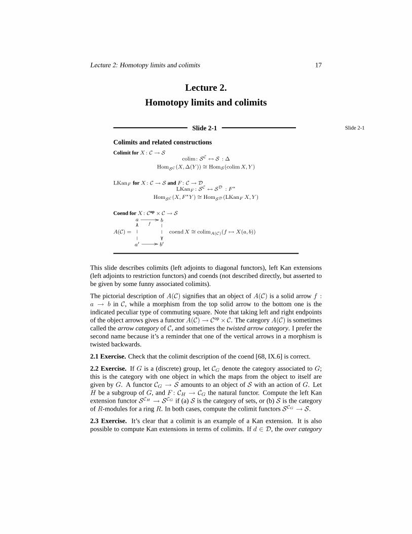
This slide describes colimits (left adjoints to diagonal functors), left Kan extensions(left adjoints to restriction functors) and coends (not described directly, but asserted tobe given by some funny associated colimits).
The pictorial description ofA(C) signifies that an object ofA(C) is a solid arrowf :a → b in C, while a morphism from the top solid arrow to the bottom one is theindicated peculiar type of commuting square. Note that taking left and right endpointsof the object arrows gives a functorA(C)→ Cop×C. The categoryA(C) is sometimescalled thearrow categoryof C, and sometimes thetwisted arrow category. I prefer thesecond name because it’s a reminder that one of the vertical arrows in a morphism istwisted backwards.
2.1 Exercise.Check that the colimit description of the coend [68, IX.6] is correct.
2.2 Exercise. If G is a (discrete) group, letCG denote the category associated toG;this is the category with one object in which the maps from the object to itself aregiven byG. A functor CG → S amounts to an object ofS with an action ofG. LetH be a subgroup ofG, andF : CH → CG the natural functor. Compute the left Kanextension functorSCH → SCG if (a) S is the category of sets, or (b)S is the categoryof R-modules for a ringR. In both cases, compute the colimit functorsSCG → S.
2.3 Exercise. It’s clear that a colimit is an example of a Kan extension. It is alsopossible to compute Kan extensions in terms of colimits. Ifd ∈ D, theover category
Lecture 2: Homotopy limits and colimits 18
(also called comma category)F↓d can be described pictorially as follows:
c, F (c)
h
''PPPPPPPPPPPPP
F (h)
d
c′, F (c′)
77nnnnnnnnnnnnn
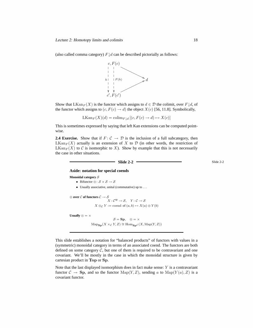
Show thatLKanF (X) is the functor which assigns tod ∈ D the colimit, overF↓d, ofthe functor which assigns to(c, F (c)→ d) the objectX(c) [56, 11.8]. Symbolically,
LKanF (X)(d) = colimF↓d [(c, F (c)→ d) 7→ X(c)]
This is sometimes expressed by saying that left Kan extensions can be computed point-wise.
2.4 Exercise. Show that ifF : C → D is the inclusion of a full subcategory, thenLKanF (X) actually is an extension ofX to D (in other words, the restriction ofLKanF (X) to C is isomorphic toX). Show by example that this is not necessarilythe case in other situations.
Slide 2-2 Slide 2-2
Aside: notation for special coends
Monoidal categoryS• Bifunctor⊗ : S × S → S• Usually associative, unital (commutative) up to. . .
⊗ over C of functors C → SX : Cop→ S, Y : C → S
X ⊗C Y := coend of (a, b) 7→ X(a)⊗ Y (b)
Usually⊗ = ×S = Sp, ⊗ = ×
MapSp(X ×C Y, Z) ∼= HomSpC (X, Map(Y, Z))
This slide establishes a notation for “balanced products” of functors with values in a(symmetric) monoidal category in terms of an associated coend. The functors are bothdefined on some categoryC, but one of them is required to be contravariant and onecovariant. We’ll be mostly in the case in which the monoidal structure is given bycartesian product inTop or Sp.
Note that the last displayed isomorphism does in fact make sense:Y is a contravariantfunctor C → Sp, and so the functorMap(Y, Z), sendinga to Map(Y (a), Z) is acovariant functor.
Lecture 2: Homotopy limits and colimits 19
2.5 Exercise. Convince yourself that the last displayed isomorphism on the slide iscorrect.
2.6 Exercise.Try to interpret the tensor product of a left module over a ringR witha right module as a coend in the above sense. It may be necessary to deal with addi-tive categories (= morphisms are abelian groups, composition is bilinear) and additivemaps between them.
2.7 Exercise. Let G be a discrete group with associated categoryCG (2.2). LetX : CG → Sp be a contravariant functor (a rightG-space) andY : CG → Sp a co-variant functor (a leftG-space). Show thatX ×CG
Y is the orbit space of action ofGon X × Y obtained by converting the action onX to a left action usingg 7→ g−1 andthen taking the diagonal action on the product.
Slide 2-3 Slide 2-3
Homotopy colimits and related constructionsC, S homotopy theories
Homotopy colimit for X : C → Shocolim: SC ↔ S : ∆
HomhSC (X, ∆(Y )) ∼ Homh
S(hocolim X, Y )
LKanhF for X : C → S and F : C → D
LKanhF : SC ↔ SD : F ∗
HomhSC (X, F ∗Y ) ∼= Homh
SD (LKanhF X, Y )
Homotopy coend forX : Cop × C → Shocoend X = hocolimA(C) of (a→ b) 7→ X(a, b)
U ⊗hC V = hocolimA(C) of (a→ b) 7→ U(a)⊗ V (b)
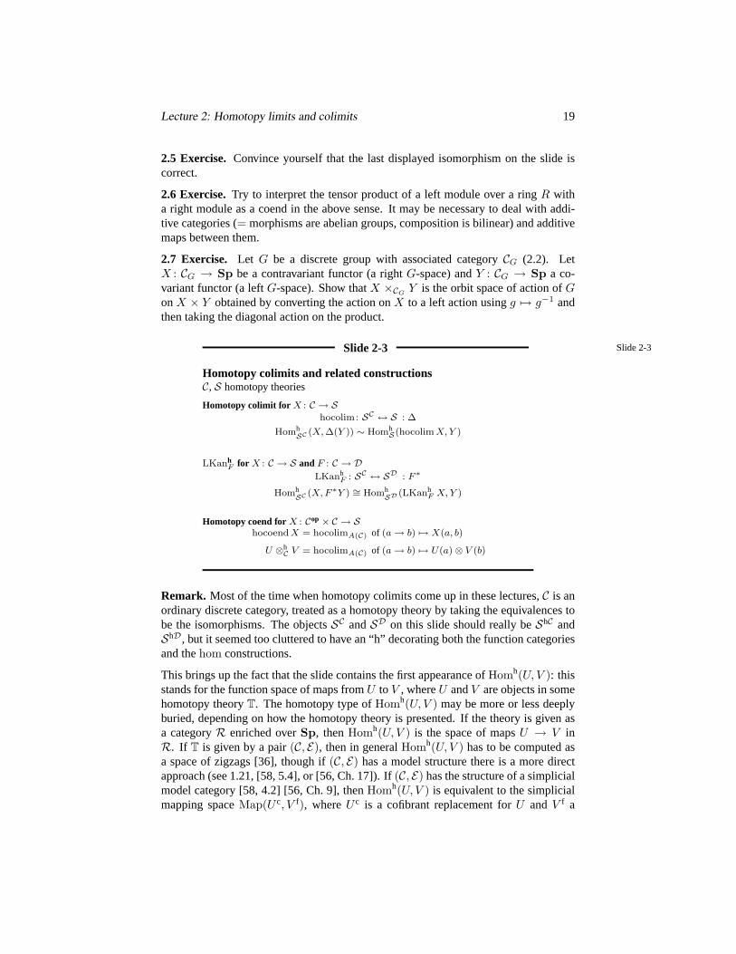
Remark. Most of the time when homotopy colimits come up in these lectures,C is anordinary discrete category, treated as a homotopy theory by taking the equivalences tobe the isomorphisms. The objectsSC andSD on this slide should really beShC andShD, but it seemed too cluttered to have an “h” decorating both the function categoriesand thehom constructions.
This brings up the fact that the slide contains the first appearance ofHomh(U, V ): thisstands for the function space of maps fromU to V , whereU andV are objects in somehomotopy theoryT. The homotopy type ofHomh(U, V ) may be more or less deeplyburied, depending on how the homotopy theory is presented. If the theory is given asa categoryR enriched overSp, thenHomh(U, V ) is the space of mapsU → V inR. If T is given by a pair(C, E), then in generalHomh(U, V ) has to be computed asa space of zigzags [36], though if(C, E) has a model structure there is a more directapproach (see 1.21, [58, 5.4], or [56, Ch. 17]). If(C, E) has the structure of a simplicialmodel category [58, 4.2] [56, Ch. 9], thenHomh(U, V ) is equivalent to the simplicialmapping spaceMap(U c, V f), whereU c is a cofibrant replacement forU and V f a

Lecture 2: Homotopy limits and colimits 20
fibrant replacement forV . In practice,Homh(U, V ) is usually given by any reasonablemapping space construction that respects equivalences in both variables.
The last displayed definition contains an underlying assumption that the pairing mapS×S → S is a map of homotopy theories (or, ifS is a category with equivalences, canbe suitably adjusted to become a map of homotopy theories). This won’t be an issuefor us, since in the monoidal category(Sp,×) the monoidal operation× does preserveequivalences.
2.8 Exercise.Explain whatX ⊗hC Y should mean ifX andY are, respectively,
contravariant and covariant functors fromC to the category of chain complexesof modules over a commutative ringR.
Note. The adjunctions above are in the appropriate enriched category sense; for in-stance the second one asserts that the two functors
HomhSC (X, F ∗Y ) and Homh
SD (LKanhF X, Y )
are explicitly equivalent as functors
(SC)op× SD → Sp .
Depending on the model for homotopy theories that is currently on the workbench, thisexplicit equivalence may or may not be realized by a direct morphism in the functorcategory; it may well be specified as a zigzag of morphisms which are direct equiva-lences.
Slide 2-4 Slide 2-4
Model category dividend
TheoremIf S admits a model category structure:
Existencehocolim, LKanh
F , hocoend exist for targetS.
Realizability• hocolim ∼ functorSC → S,
• LKanhF ∼ functorSC → SD , and
• hocoend ∼ functorSCop×C → S.
Remark. This theorem may or may not have been proved in the form in which it’sstated, but it’s certainly true. The only issue is whether the various constructions avail-able have been explicitly identified as homotopy colimits (etc.) in the sense of theprevious slide.

Lecture 2: Homotopy limits and colimits 21
Slide 2-5 Slide 2-5
Construction of hocolim, version I
Assumptions• S admits a model structure
• SC admits the projective model structure(fibrations are objectwise)
The assumptions hold ifS is Sp, orTop.
Conclusionhocolim X ∼ colim Xc, X ∈ SC
The assumptions hold ifC is an increasing category (1.26) or ifS admits a cofibrantlygenerated model category structure. For instance, the above technique always works forcomputing homotopy pushouts (1.24; see [41,§10]). Every object inSp is cofibrant,so a homotopy pushout inSp can be calculated by converting the two maps involvedinto cofibrations (leaving the common domain unchanged) and then taking a pushout.
2.9 Exercise. Give an example to show that in(Tophe)∗ (the categoryof pointed topological spaces with pointed homotopy equivalences as the
equivalences) the coproduct of two objects is not necessarily equivalent to the homo-topy coproduct of the objects. (Even coproducts sometimes have to be derived.)
2.10 Exercise.Look ahead to slide 2–9. Can you think of an example in which theproduct of a collection of objects in a model category is not equivalent to their homo-topy product (the product of their fibrant replacements)?
2.11 Exercise. How about an example different from the one you got byapplying the “opposite category” trick to 2.9 .
Slide 2-6 Slide 2-6
Construction of hocolim, version IITop, Sp. . . .
(A) |Y | for Y : ∆op→ Top or Sp
|Y | =(
∆∗ ×∆op Y for Top
∆[∗]×∆op Y for Sp
(B) Repl∗(X) : ∆op→ S for X : C → SRepl∗(X)(n) =
af : 0→1→···→n→C
f(0)
hocolim = (A) + (B)hocolim X ∼ |Repl∗(X)|

Lecture 2: Homotopy limits and colimits 22
Note. The functor∆∗ is the functor∆→ Top which sends the setn to the geometricn-simplex∆n (the space of convex linear combinations of points inn. Similarly,∆[∗]is the functor∆ → Sp which sendsn to the simplicial set∆[n] corresponding tothen-simplex, considered as an ordered simplicial complex.Repl∗(X) is called thesimplicial replacementof the diagramX [18, XII].
2.12 Remark. This construction of the homotopy colimit works in many simplicialmodel categories. Sometimes it’s a good idea to insist that the values of the functorXare cofibrant objects in the base category; this guarantees the coproducts which enterinto the formation ofRepl∗(X) have the correct equivalence type and that the gluinginvolved in the realization construction is well-behaved. It is something of a surprisethat this cofibrancy condition is not necessary inTop [30]. It is necessary inTop∗(2.9).
Remark. In general, it is necessary to be careful in forming the realization of anarbitrary simplicial object in a simplicial model category. (If youare careful, the re-alization of the simplicial object should be equivalent to its homotopy colimit as afunctor∆op→ S.) Being careful in this case means checking to see that the simplicialobject is Reedy cofibrant [58, 5.2] [49, VII]. Roughly, “Reedy cofibrant” means thatcombined images of the degeneracy maps at each level sit cofibrantly inside the objectat that level, a request which is not unreasonable, since taking the realization involvescollapsing out the images of the degeneracy maps. Every simplicial object inSp isReedy cofibrant, but the same is not true of every simplicial object inTop; this leadsto the tale of the thick realization of a simplicial topological space [91, Appendix].
2.13 Exercise. Check that the above simplicial construction does in fact give a ho-motopy pushout inTop which agrees up to equivalence with the sort of homotopypushout from slide 2–5. (The outcome of the simplicial construction isn’t nearly aselaborate as it might look. Realizing a simplicial object involves collapsing the imagesof degeneracy maps, and almost all of the pieces of the simplicial replacement for apushout diagram are degenerate.)
2.14 Exercise.Verify that the simplicial set∆[n] is the functor∆op → Set whichsendsm to Hom∆(m,n). Conclude that for any simplicial setX, HomSp(∆[n], X)is naturally isomorphic toXn.
? 2.15 Exercise.The following is not hard to prove, but it is completely implausibleat first sight. The coend formula for the realization of a simplicial objectX∗ in Spexhibits|X∗| as a quotient
|X∗| =∐n
(∆[n]×Xn) / ∼
where in this case∼ is an equivalence relation generated by the morphisms in∆op.But X∗ is just a simplicial object in the category of simplicial sets, as such it amountsto a functor
X : ∆op→ Set∆op
or X : : ∆op×∆op→ Set
Lecture 2: Homotopy limits and colimits 23
The second way of looking atX leads to the definition of the diagonaldiag(X); thisis the simplicial set
diag(X) : ∆op diag−−→∆op×∆op X−→ Set .
Prove that for any simplicial objectX in Sp, |X| is isomorphic todiag(X).
2.16 Exercise.In Top, interpret the above simplicial homotopy colimit ofX → Yas the mapping cylinder of the map. What’s the (simplicial ) homotopy colimit ofX → Y → Z? Interpret a homotopy colimit inTop indexed by an arbitrary categoryin terms of building blocks of this kind [18, XII.2].
? 2.17 Exercise.Verify that the nerve (1.7) of a categoryC can be identified as thehomotopy colimit of the constant functor which assigns to each object ofC the one-point space. The constant functor is treated as taking values inSp, and the homotopycolimit is in Sp.
2.18 Exercise.The above construction of the homotopy colimit works for the categorySp∗ of pointed simplicial sets (and also in the categoryTop∗ of pointed spaces, aslong as the values of the functorX are assumed to be cofibrant, see 2.12). Verify thatthe homotopy colimit in the pointed category is obtained by forming the homotopycolimit in the unpointed category and collapsing out the nerve of the index category(i.e., the unpointed homotopy colimit of the one-point basepoint functor).
2.19 Exercise.Draw a picture of a homotopy coequalizer inTop.
2.20 Exercise. Filtering ∆∗ or ∆[∗] by skeleta gives an increasing fil-tration of hocolim X, which leads to a homology spectral sequence for
h∗(hocolim X) (hereh∗ is any homology theory). Identify theE2 page of the spectralsequence as
E2(i, j) = colimi hj(X)
wherecolimi is thei’th (classical) left derived functor of the colimit functorAbC →Ab andhj(X) is the functorC → Ab obtained by applyinghj to X.
2.21 Exercise.In the above situation, show that theE2 page can be identifiedmore explicitly as
E2(i, j) = HiN(hj(Repl∗(X))) .
Herehj(Repl∗(X)) is the simplicial abelian group obtained fromRepl∗(X) by apply-ing Ej , N is normalization as in (1.13), andHi is thei’th homology group of a chaincomplex.
2.22 Exercise. In an exercise that, in light of the above two, might seemobscurely confusing, show that ifA ∈ Ab∆op
is a simplicial abelian group,then
colimi A ∼= HiN(A) .
Resolve the confusion by observing that ifB : C → Ab is any functor,colim∗(B) canbe computed by a simplicial replacement formula.

Lecture 2: Homotopy limits and colimits 24
Slide 2-7 Slide 2-7
Homotopy limits and related constructionsC, S homotopy theories
Homotopy limit for X : C → S∆: S ↔ SC : holim
HomhSC (∆(Y ), X) ∼ Homh
S(Y, holim X)
RKanhF for X : C → S and F : C → D
F ∗ : SD ↔ SC : RKanhF
HomhSC (F ∗Y, X) ∼= Homh
SD (Y, RKanhF X)
Homotopy end for X : Cop × C → Shoend X = holimA(C) of (a→ b) 7→ X(a, b)
Remark. The opposite of a homotopy theory is a homotopy theory, so a hapless lec-turer who was pressed for time could point out that homotopy limits are just homotopycolimits in the opposite category, and leave it at that. . .
In this slide, as in 2–3,SC andSD should really beShC andShD
2.23 Exercise.Formulate the notion of right Kan extension, and show that right Kanextensions can be computed pointwise (2.3). It will probably be necessary to considertheunder categoriesd↓F :
F (c), c
h
F (h)
d
77nnnnnnnnnnnnn
''PPPPPPPPPPPPP
F (c′), c′
Identify some interesting right Kan extension.
2.24 Exercise.If X, Y : C → S are two functors between ordinary categories, there isa functorHX,Y : Cop× C → Set given by
HX,Y (c, c′) = HomS(X(c), Y (c′)) .
Check that the end of this functor is isomorphic toHomSC (X, Y ).
Remark. Suppose thatC andS are homotopy theories. The mapping theoryShC isdefined so that ifX, Y : C → S are objects of the theory, then
HomhSC(X,Y ) ∼ hoendC
[(c, c′) 7→ Homh
S(X(c), Y (c′))]
.

Lecture 2: Homotopy limits and colimits 25
Slide 2-8 Slide 2-8
Another model category dividend
TheoremIf S admits a model category structure:
Existenceholim, RKanh
F , hoend exist for targetS.
Realizability• holim ∼ functorSC → S,
• RKanhF ∼ functorSC → SD , and
• hoend ∼ functorSCop×C → S.
Remark. This really does follow from the corresponding remark about homotopycolimits, etc., because the notion of a model category is self-dual (1.18).
Slide 2-9 Slide 2-9
Construction of holim, version I
Assumptions• S admits a model structure
• SC admits the injective model structure(cofibrations are objectwise)
The assumptions hold ifS is Sp (Top?)
Conclusionholim X ∼ lim X f , X ∈ SC
? 2.25 Exercise.Determine what this says about homotopy pullbacks inSp orTop.What do you need to do to compute the homotopy limit of a tower
· · · → Xn → Xn−1 → · · ·X1 → X0
in a model category.
Lecture 2: Homotopy limits and colimits 26
Slide 2-10 Slide 2-10
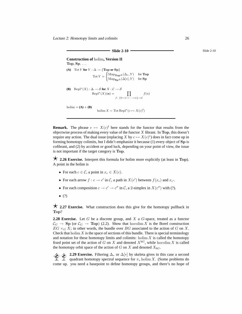
Construction of holim, Version IITop, Sp. . . .
(A) Tot Y for Y : ∆→ Top or Sp
Tot Y =
(MapTop∆ (∆∗, Y ) for Top
MapSp∆ (∆[∗], Y ) for Sp
(B) Repl∗(X) : ∆→ S for X : C → SRepl∗(X)(n) =
Yf : 0→1→···→n→C
f(n)
holim = (A) + (B)holim X ∼ TotRepl∗(c 7→ X(c)f)
Remark. The phrasec 7→ X(c)f here stands for the functor that results from theobjectwise process of making every value of the functorX fibrant. InTop, this doesn’trequire any action. The dual issue (replacingX by c 7→ X(c)c) does in fact come up informing homotopy colimits, but I didn’t emphasize it because (1) every object ofSp iscofibrant, and (2) by accident or good luck, depending on your point of view, the issueis not important if the target category isTop.
? 2.26 Exercise.Interpret this formula for holim more explicitly (at least inTop).A point in the holim is
• For eachc ∈ C, a point inxc ∈ X(c).
• For each arrowf : c→ c′ in C, a path inX(c′) betweenf(xc) andxc′ .
• For each compositionc→ c′ → c′′ in C, a2-simplex inX(c′′) with (?).
• (?)
? 2.27 Exercise. What construction does this give for the homotopy pullback inTop?
2.28 Exercise. Let G be a discrete group, andX a G-space, treated as a functorCG → Sp (or CG → Top) (2.2). Show thathocolim X is the Borel constructionEG ×G X; in other words, the bundle overBG associated to the action ofG on X.Check thatholim X is the space of sections of this bundle. There is special terminologyand notation for these homotopy limits and colimits:holim X is called the homotopyfixed point set of the action ofG on X and denotedXhG, while hocolim X is calledthe homotopy orbit space of the action ofG onX and denotedXhG.
2.29 Exercise.Filtering ∆∗ or ∆[∗] by skeleta gives in this case a secondquadrant homotopy spectral sequence forπ∗ holim X. (Some problems do
come up. you need a basepoint to define homotopy groups, and there’s no hope of
Lecture 2: Homotopy limits and colimits 27
choosing a basepoint if for instanceholim X is empty. So assume thatX is a diagramof pointed objects to guarantee a distinguished point inholim X.) Compare this with2.20. Show that theE2 page of the spectral sequence is given by
E2(−i, j) = limi πjX
where limi is the i’th right derived functor oflim: AbC → Ab. Or maybe not;remember thatπ0 is just a set, whileπ1 is a possibly nonabelian group. This spectralsequence might occupy more second quadrant than you expect [14].
Slide 2-11 Slide 2-11
Properties of homotopy (co)limitsfor functorsC → SUniversal maps
hocolim X → colim X
lim X → holim X
Homotopy invariance
X ∼→ Y =⇒(
hocolim X ∼→ hocolim Y
holim X ∼→ holim Y
Mapping adjointnessHomh
S(hocolim X, Y ) ∼ holimCop of c 7→ Homh(X(c), Y )
HomhS(Y, holim X) ∼ holimC of c 7→ Homh(Y, X(c))
Remark. The two homotopy limits on the right in the last display are homotopy limitsof functors intoSp (or Top).
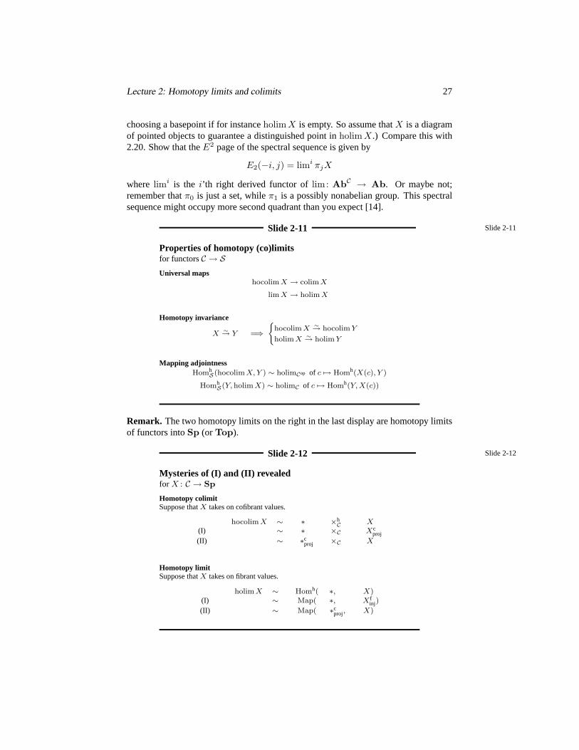
Slide 2-12 Slide 2-12
Mysteries of (I) and (II) revealedfor X : C → Sp
Homotopy colimitSuppose thatX takes on cofibrant values.
hocolim X ∼ ∗ ×hC X
(I) ∼ ∗ ×C Xcproj
(II) ∼ ∗cproj ×C X
Homotopy limitSuppose thatX takes on fibrant values.
holim X ∼ Homh( ∗, X)(I) ∼ Map( ∗, X f
inj)
(II) ∼ Map( ∗cproj, X)

Lecture 2: Homotopy limits and colimits 28
This is a lot like homological algebra: if you want to compute the derived tensor prod-uct of two chain complexes, you can make either one or the other projective, it doesn’tmatter which.
Remark. In the first box,∗ is a contravariant constant functor, and in the secondbox it’s a covariant one. The simplicial formula forhocolim X arises from taking thefollowing cofibrant model for∗ in the projective model category structure onSpC
op
:
(∗cproj)(x) = N(x↓C) .
See 2.23 for a description of the under categoryc↓C; for brevity,C here stands for theidentify functor onC.
2.30 Exercise.Check that this formula does provide a cofibrant model for∗, and that(∗c
proj)×C X does in fact describe the simplicial model forhocolim X.
In the second box,Map stands for the simplicial mapping complex and∗cproj is a cofi-
brant model for∗ in the projective model category structure onSpC . The cosimplicialformula forholim X arises from taking the cofibrant model given by
(∗cproj)(x) = N(C↓x) .
Lecture 3: Spaces from categories 29
Lecture 3.
Spaces from categories
In this section we’ll look at various constructions on categories which give interestingresults when the nerve functor is applied. At then end there’s a short discussion ofterminal functors and initial functors (generalization of terminal objects and initial ob-jects). The basic properties of these functors don’t directly involve nerves of categories,but the functors are tied to nerves in a couple of different ways.
Slide 3-1 Slide 3-1
Categories vs. Spaces
GeometrizationN : Cat→ Sp
Properties• F : C → D 7→ N F : N C → ND• τ : F
.→ G 7→ H : N C ×∆[1]→ D
Advantages
• Categories more visible than spaces.
• Natural transformations more accessible than homotopies.
Can homotopy colimits (coends) be built in?F : C → Cat =⇒ hocolimC N(F ) ∼ N(?)
It is pretty clear that ifC is a category then the nerveN C of C, considered up to equiv-alence inSp, does not capture a lot of the structure inC.
3.1 Exercise.Give an example of two categoriesC andD such thatN C andND areequivalent (i.e. weakly homotopy equivalent) as simplicial sets, but such thatC andDare not equivalent as categories.
But there is something to be said.
3.2 Exercise. Show thatN C andND are weakly equivalent as simplicialsets if and only if the category pairs(C, C) and(D,D) give equivalent ho-
motopy theories. (In other words, the nerveN C, considered up to the usual notion ofequivalence for simplicial sets, exactly captures the homotopy theory that results frominverting all of the arrows inC.)
3.3 Exercise.Show thatN C, considered up to isomorphism of simplicial sets,determinesC up to isomorphism of categories. (Hint: look at the left adjoint to
N : Cat→ Sp).
Trying to interpolate between the previous two exercises might well lead to the notionof a quasicategory.
Lecture 3: Spaces from categories 30
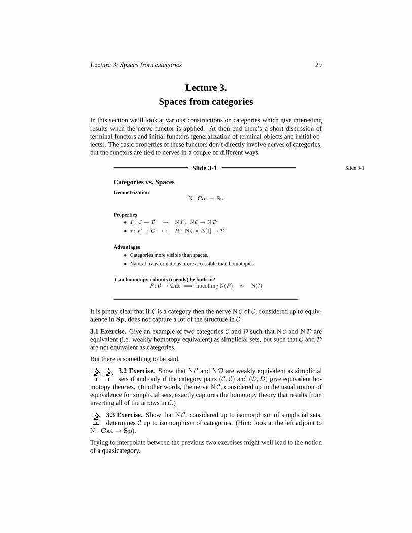
Slide 3-2 Slide 3-2
The Grothendieck ConstructionF : C → Cat =⇒ categoryCnF
x
•
c
Object Morphism
x
•
c
im(x)
x′
••
jjjj44
c′___________ //f
____ //F (f)
The Grothendieck constructionCnF is also denotedC oF ,∫C F , or in general anything
else that somehow connotes adding up the values ofF overC. The slide is supposed toindicate that an object of the categoryCnF is a pair(c, x), wherec ∈ C andx ∈ F (c);a morphism(c, x) → (c′, x′) is then a pair(f, g), wheref is a morphismc → c′ in Candg is a morphismF (f)(x)→ x′ in F (c′).
3.4 Exercise.Suppose thatF is the constant functorC → Cat with valueD. ShowthatCnF is the product categoryC × D.
3.5 Exercise.Suppose that the groupG acts on the groupH by automorphisms, andlet F : CG → Grp be the corresponding functor (2.2). Show thatCnF is the categorycorresponding to the semidirect product groupG n H. (The intent here is that then symbol is oriented so that the closed triangle points sideways towards the normalsubgroup.)
Slide 3-3 Slide 3-3
Thomason’s TheoremF : C → Cat
TheoremN(CnF ) ∼ hocolimC N(F )
ExampleF : C → Set, CnF = Transport Category• Object: (c, x), c ∈ C, x ∈ F (c)
• Morphism: f : c→ c′ with f(x) = x′
N(Transport Category) ∼ hocolim F
Lecture 3: Spaces from categories 31
The reference for Thomason’s theorem is [97].
3.6 Exercise. In the above situation, show that the nerve of the transport category isactually isomorphic tohocolim F , wherehocolim F is formed according to the sim-plicial formula.
3.7 Exercise.Consider the possibility thatCnF might be the homotopy col-imit of F in the category of homotopy theories. Can you find any evidence
for or against this suggestion? Is there any reason to believe that the nerve functor fromcategories to simplicial sets should commute with (homotopy) colimits?
Slide 3-4 Slide 3-4
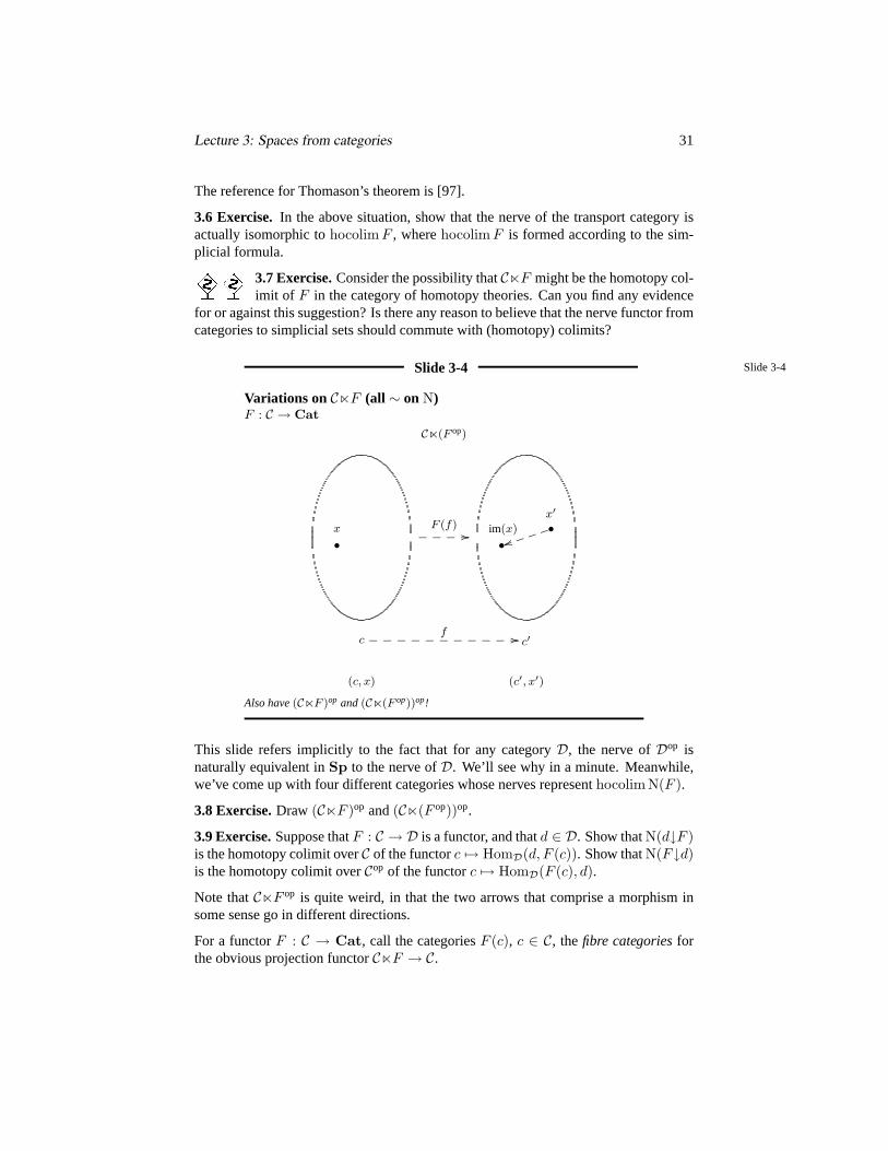
Variations on CnF (all ∼ on N)F : C → Cat
Cn(F op)
x
•
c
(c, x)
im(x)
x′
•j j j jtt•
c′
(c′, x′)
___________ //f
____ //F (f)
Also have(CnF )op and(Cn(F op))op!
This slide refers implicitly to the fact that for any categoryD, the nerve ofDop isnaturally equivalent inSp to the nerve ofD. We’ll see why in a minute. Meanwhile,we’ve come up with four different categories whose nerves representhocolim N(F ).
3.8 Exercise.Draw (CnF )op and(Cn(F op))op.
3.9 Exercise.Suppose thatF : C → D is a functor, and thatd ∈ D. Show thatN(d↓F )is the homotopy colimit overC of the functorc 7→ HomD(d, F (c)). Show thatN(F↓d)is the homotopy colimit overCop of the functorc 7→ HomD(F (c), d).
Note thatCnF op is quite weird, in that the two arrows that comprise a morphism insome sense go in different directions.
For a functorF : C → Cat, call the categoriesF (c), c ∈ C, thefibre categoriesforthe obvious projection functorCnF → C.

Lecture 3: Spaces from categories 32
3.10 Exercise.Show that if all of these fibre categories have contractible nerve, then theprojectionN(CnF ) → N(C) is an equivalence of simplicial sets. (Use the homotopyinvariance of homotopy colimits, the fact that the nerve ofC is hocolimC ∗, and somesort of functoriality which I haven’t stated but which must be built into Thomason’stheorem.)
3.11 Exercise.Show that adjoint functors
F : C ↔ D : G
induce inverse equivalences (up to homotopy) betweenN C andND. Hint: naturaltransformations give homotopies (1.8). Deduce (again 1.9) that any category with aninitial object or a terminal object has a contractible nerve.
Recall that ifC is a category,A(C) stands for the twisted arrow category ofC (2.1).There are natural functorsA(C)→ C andA(C)→ Cop.
? 3.12 Exercise.Show thatA(C) → C can be identified asCnF → C for somefunctor C → Cat. Observe that all of the fibre categories have contractible nerves.Show that the same is true ofA(C)→ Cop. Conclude that in the diagram
C ← A(C)→ Cop
both of the functors induce equivalences on nerves [85, p. 94].
Slide 3-5 Slide 3-5
Extension to homotopy coendsF : C → Cat, G : Cop→ Cat N(GoCnF ) ∼ N(G)×h
C N(F )
GoCnF = (c, x, y)
Morphism
x•
x′•
•44___ //
F (f)
y•
•tt
c
y′•
c′______ //f
_ _ _ooG(f)

Lecture 3: Spaces from categories 33
There’s a discussion of the Grothendieck construction model for homotopy coendsin [36, §9]. It’s terse, and I don’t thing the phrase “homotopy coend”’ appears any-where, but the argument does produce an equivalence between the nerve of a two-sidedGrothendieck construction and a simplicial model for the homotopy coend along thelines of slide 2–6.
The slide signifies that an object ofGoCnF is a triple(c, x, y) wherec ∈ C, x ∈ F (c),andy ∈ G(c). A morphism(c, x, y)→ (c′, x′, y′) is itself a triple, consisting of a mapf : c → c′ in C, a mapF (f)(x) → x′ in F ′(c) and a mapG(f)(y′) → y in G(c). Itshould be pretty clear how to compose these triples.
The reader is left to ponder the multitudinous variants ((Gop)oCnF , GoCn(F op),. . .), all of which have equivalent nerves. One point that sometimes disorients me a bitis the fact that the opposite category construction(−)op is acovariantfunctor onCat.
Working with Grothendieck constructions can be unexpectedly tricky. Here’s an exam-ple (which when sorted out leads to yet larger collections of categories with equivalentnerves). Suppose thatC is category with equivalencesE (i.e. a homotopy theory) andthatx andy are objects ofC. Consider the diagram categoryZiZaZig(x, y) describedby the following picture:
A∼
~~~~~~
~~~~
//
∼
B
∼
x y
∼``@@@@@@@@
∼~~
~~~~
~~
A′
∼
__@@@@@@@@// B′
The solid arrow zigzags are the objects of the category, and the pictured commuta-tive diagram (which includes the dashed arrows) gives a morphism between the upperzigzag and the lower one. The problem is to understand the homotopy type of the nerveof this category. There are several ways to take this homotopy type apart; the most sym-metrical one is to observe that an object consists of a triple(U, V, h), whereU : A→ xis an object of the over categoryE↓x, V : y → B is an object of the under categoryy↓E , andh is an element ofF (U, V ) = HomC(A,B). The functorF is contravariantin U , covariant inV , and takes values in sets (= discrete categories). A morphism(U, V, h)→ (U ′, V ′, h′) in ZiZaZig(x, y) consists of a morphismu : U → U ′ in E↓xand a morphismv : V → V ′ in y↓E such thatu∗(h′) = v∗(h) (this is the commutativ-ity of the central square).
A first guess based on looking at the variances might have
ZiZaZig(x, y) ∼= DnF for D = (E↓x)op× (y↓E)
but this would be hasty.
Lecture 3: Spaces from categories 34
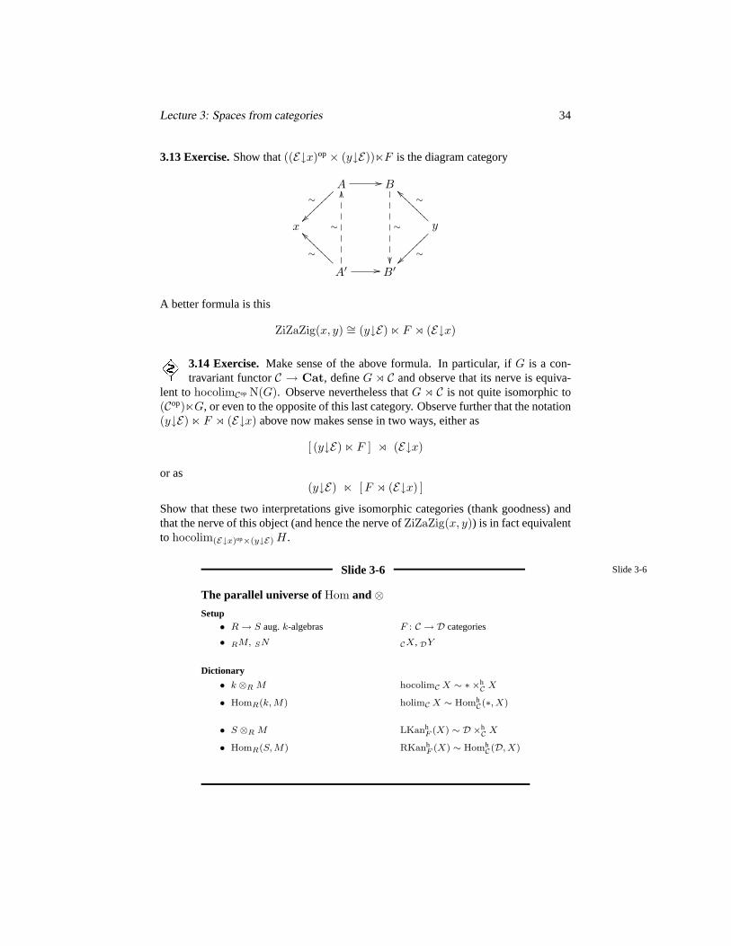
3.13 Exercise.Show that((E↓x)op× (y↓E))nF is the diagram category
A∼
~~~~~~
~~~~
// B
∼
x y
∼``@@@@@@@@
∼~~
~~~~
~~
A′
∼
__@@@@@@@@
∼
OO
// B′
A better formula is this
ZiZaZig(x, y) ∼= (y↓E) n F o (E↓x)
3.14 Exercise.Make sense of the above formula. In particular, ifG is a con-travariant functorC → Cat, defineG o C and observe that its nerve is equiva-
lent tohocolimCop N(G). Observe nevertheless thatG o C is not quite isomorphic to(Cop)nG, or even to the opposite of this last category. Observe further that the notation(y↓E) n F o (E↓x) above now makes sense in two ways, either as
[ (y↓E) n F ] o (E↓x)
or as(y↓E) n [F o (E↓x) ]
Show that these two interpretations give isomorphic categories (thank goodness) andthat the nerve of this object (and hence the nerve ofZiZaZig(x, y)) is in fact equivalentto hocolim(E↓x)op×(y↓E) H.
Slide 3-6 Slide 3-6
The parallel universe ofHom and⊗Setup• R→ S aug.k-algebras F : C → D categories
• RM, SN CX, DY
Dictionary
• k ⊗R M hocolimC X ∼ ∗ ×hC X
• HomR(k, M) holimC X ∼ HomhC(∗, X)
• S ⊗R M LKanhF (X) ∼ D ×h
C X
• HomR(S, M) RKanhF (X) ∼ Homh
C(D, X)
Lecture 3: Spaces from categories 35
At this point we’re beginning to work our way towards some preliminary applicationsof the Grothendieck construction; more applications will come up later on.
The notationCX on this slide denotes for short thatX is a covariant functor fromCto, say,Sp. In the notationD ×h
C X, D is shorthand for the contravariant functorC → SetD given by
c 7→ HomD(F (c),−) .
(Note that the object on the right actually is a functor fromD to Set.) The indicatedhomotopy coend can be computed objectwise inD; in symbols
(D ×hC X)(d) = HomD(F (−), d)×h
C X .
The fact thatD stands for aD Hom-functor which is contravariant onC is silentlyimplied by the fact thatD appears on the left side of the homotopy coend.
Similarly, HomhC(D, X) stands for the functorD → Sp which sendsd to
HomhC(HomD(d, F (−)), X) .
The fact thatD here represents a covariantHom-functor onC is necessitated by the factthatD appears inside of aHomh construction in which the second component, namelyX, is covariant.
The parallel universes here involve two constructions (restriction of a module along aring homomorphism, pullback of a diagram along a functor), each of which has bothleft and right adjoints. In both cases there’s an underlying homotopy theory (at least ifyou replace modules over the rings by chain complexes of modules) and both the leftadjoint and the right adjoint can be usefully derived (although the slide doesn’t refer tothe possibility of deriving the algebraic constructions). The main point of the slide ispsychological rather than mathematical: if you use notation for left and right homotopyKan extensions which is similar to familiar algebraic notation, you find yourself led tocorrect conclusions.
3.15 Exercise.Find some reason to believe that the indicated formulas for theright and left homotopy Kan extensions are correct.
For the material on the next few slides, see [57] or [39,§9].
Lecture 3: Spaces from categories 36
Slide 3-7 Slide 3-7
Properties of Kan extensions
Transitivity (pushing forward over functors)M, R // 33S // T X, C // 33D // S
On the leftAlgebra T ⊗R M ∼= T ⊗S S ⊗R M
Topology S ×hC X ∼ S ×h
D D ×hC X
On the right
Algebra HomR(T, M) ∼= HomS(T, HomR(S, M))
Topology HomhC(S, X) ∼ Homh
D(S, HomhC(D, X))
3.16 Exercise.What does this transitivity say about homotopy colimits?
3.17 Exercise.Check the transitivity properties by using adjointness properties of thehomotopy Kan extensions.
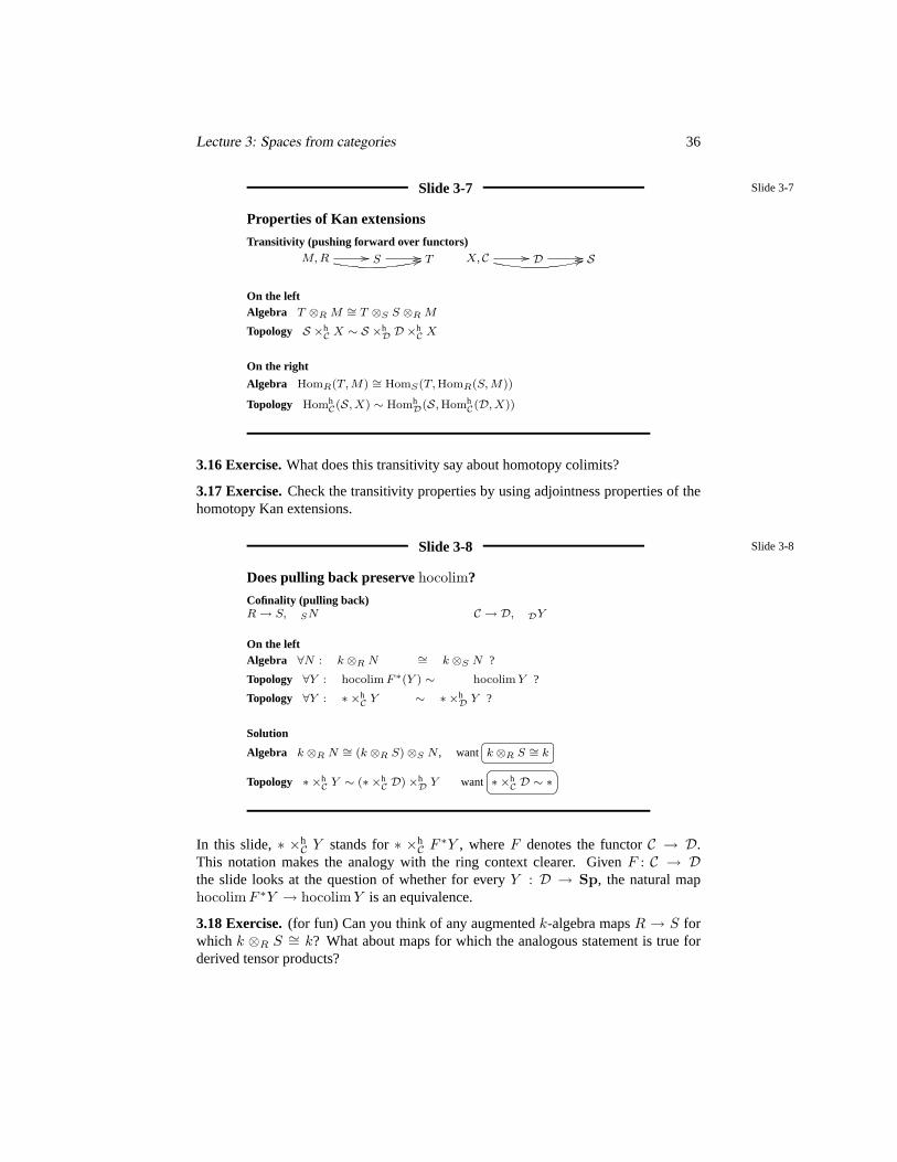
Slide 3-8 Slide 3-8
Does pulling back preservehocolim?
Cofinality (pulling back)R→ S, SN C → D, DY
On the leftAlgebra ∀N : k ⊗R N ∼= k ⊗S N ?
Topology ∀Y : hocolim F ∗(Y ) ∼ hocolim Y ?
Topology ∀Y : ∗ ×hC Y ∼ ∗ ×h
D Y ?
Solution
Algebra k ⊗R N ∼= (k ⊗R S)⊗S N , want k ⊗R S ∼= k
Topology ∗ ×hC Y ∼ (∗ ×h
C D)×hD Y want
∗ ×hC D ∼ ∗
In this slide,∗ ×hC Y stands for∗ ×h
C F ∗Y , whereF denotes the functorC → D.This notation makes the analogy with the ring context clearer. GivenF : C → Dthe slide looks at the question of whether for everyY : D → Sp, the natural maphocolim F ∗Y → hocolim Y is an equivalence.
3.18 Exercise.(for fun) Can you think of any augmentedk-algebra mapsR → S forwhich k ⊗R S ∼= k? What about maps for which the analogous statement is true forderived tensor products?

Lecture 3: Spaces from categories 37
Slide 3-9 Slide 3-9
Terminal functorsDefinition 3. F : C → D terminal if ∗ ×h
C D ∼ ∗.
TheoremF : C → D terminal,DY =⇒ hocolimC Y ∼ hocolimD Y
Interpretation (Grothendieck construction!)
(∗ ×hC D)(d) = N(d↓F )
F (c), c
h
F (h)
d
77nnnnnnnnnnnnn
''PPPPPPPPPPPPP
F (c′), c′
This theorem guarantees that if for eachd ∈ D the under categoryd↓F has a con-tractible nerve, thenF : C → D preserves homotopy colimits (in other words, for eachY : D → Sp, hocolim F ∗Y ∼ hocolim Y .
3.19 Exercise.Prove that this is an if and only if condition. Hint: consider the functorsonD given byHomD(d,−) for variousd. Show that each one has a contractible homo-topy colimit (use the Grothendieck construction to interpret this in category theoreticalterms). Investigate what it means forF ∗ HomD(d,−) to have a contractible homotopycolimit.
3.20 Exercise.(Sanity check.) Show that ifτ is a terminal object of a categoryC, thenthe inclusionτ → C is a terminal functor.
3.21 Exercise.GivenF : C → D, prove that if for eachd ∈ D the nerve ofd↓F isconnected, thenF preserves arbitrary colimits. Is this an if and only if statement?
3.22 Exercise.Prove Quillen’s Theorem A, which states that ifF : C → D is a functorwith the property that for eachd ∈ D the under categoryd↓F has nerve equivalent toa point, thenF induces an equivalence on nerves.
Somewhat trickier is Quillen’s Theorem B, which states the following. Suppose thatthe nerve ofD is connected (to make the statement simpler) and that for each mapf : d → d′ in D the (obvious) induced mapN(d′↓F ) → N(d↓F ) is an equivalence.Then the homotopy fibre of the mapN(C) → N(D) is equivalent toN(d↓F ) for anyd ∈ D. Assume the following statement:
Theorem 3.23. Suppose thatN(D) is connected, and thatF : D → Sp is a functorwhich takes each morphism ofD to an equivalence inSp. Then the homotopy fibre ofthe natural maphocolimD F → hocolimD ∗ = N(D) is equivalent in a natural wayto F (d) for anyd ∈ D.
Lecture 3: Spaces from categories 38
3.24 Exercise.Given Theorem 3.23, prove Quillen’s Theorem B. Do this by takingthe Grothendieck construction of the functord 7→ (d↓F ) onDop and arguing that forcategorical reasons (natural transformations, adjoint functors, etc.) the nerve of thiscategory is equivalent toN(C).
3.25 Exercise.Prove another version of Quillen’s Theorem B in which the under cate-gories are replaced by over categories. (Note thatd 7→ (F↓d) gives a covariant functorD → Cat.
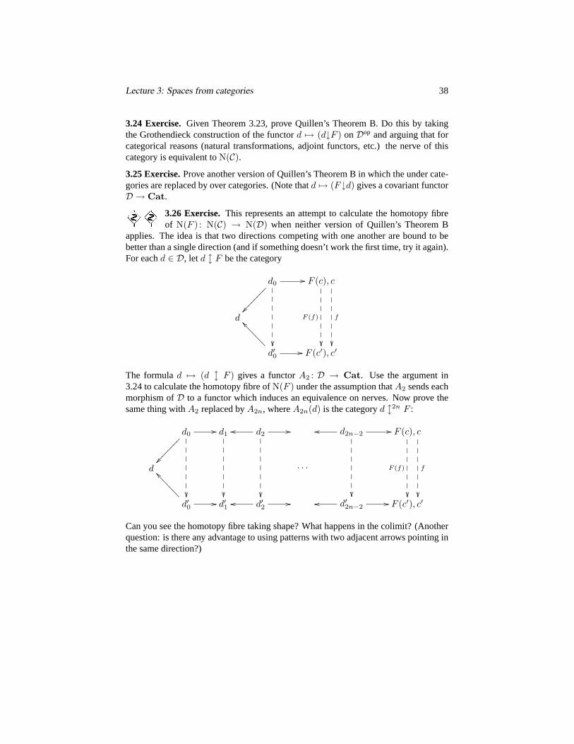
3.26 Exercise.This represents an attempt to calculate the homotopy fibreof N(F ) : N(C) → N(D) when neither version of Quillen’s Theorem B
applies. The idea is that two directions competing with one another are bound to bebetter than a single direction (and if something doesn’t work the first time, try it again).For eachd ∈ D, let d l F be the category
d0
// F (c), c
F (f)
f
d
d′0
__>>>>>>>// F (c′), c′
The formulad 7→ (d l F ) gives a functorA2 : D → Cat. Use the argument in3.24 to calculate the homotopy fibre ofN(F ) under the assumption thatA2 sends eachmorphism ofD to a functor which induces an equivalence on nerves. Now prove thesame thing withA2 replaced byA2n, whereA2n(d) is the categoryd l2n F :
d0
// d1
d2
oo
// d2n−2oo
// F (c), c
F (f)
f
d · · ·
d′0
^^>>>>>>>// d′1 d′2
oo // d′2n−2//oo F (c′), c′
Can you see the homotopy fibre taking shape? What happens in the colimit? (Anotherquestion: is there any advantage to using patterns with two adjacent arrows pointing inthe same direction?)

Lecture 3: Spaces from categories 39
Slide 3-10 Slide 3-10
Does pulling back preserveholim?
Cofinality (pulling back)R→ S, SN C → D, DY
On the rightAlgebra ∀N : HomR(k, N) ∼= HomS(k, N) ?
Topology ∀Y : holim F ∗(Y ) ∼ holim Y ?
Topology ∀Y : HomhSC (∗, Y ) ∼ Homh
SD (∗, Y ) ?
Solution
Algebra HomR(k, N) ∼= HomS(S ⊗R k, N) S ⊗R k ∼= k
Topology HomhSC (∗.Y ) ∼= Homh
SD (D ×hC ∗, Y )
D ×hC ∗ ∼ ∗
Here, givenF : C → D, the question is whether for every functorY : D → Sp, thenatural mapholim Y → holim F ∗Y is an equivalence.
Slide 3-11 Slide 3-11
Initial functorsDefinition 4. F : C → D initial if D ×h
C ∗ ∼ ∗.
TheoremF : C → D initial, DY =⇒ holimC Y ∼ holimD Y
Interpretation (Grothendieck construction again!)
(D ×hC ∗)(d) = N(F↓d)
c, F (c)
h
""FFFF
FFFF
F
F (h)
d
c′, F (c′)
<<xxxxxxxxx
3.27 Exercise.(Another sanity check.) Verify that ifι is an initial object ofD, then theinclusionι → D is an initial functor.
3.28 Exercise.Does the converse of the theorem on the slide hold? (In otherwords, if a functorF preserves all homotopy limits, isF initial?)
The theorem on the slide is Bousfield and Kan’s cofinality theorem for homotopy limits[18, XI.9.2], which they use [18, XI.10.6] to identify theR-completion as what in ourterms would be called a homotopy right Kan extension (slide 5–9).
Lecture 4: Homology decompositions 40
Lecture 4.Homology decompositions
In this lecture, we’ll use the machinery of homotopy colimits and Grothendieck con-structions to construct homology approximations for classifying spaces of finite groups.
Slide 4-1 Slide 4-1
Approximation data for BG
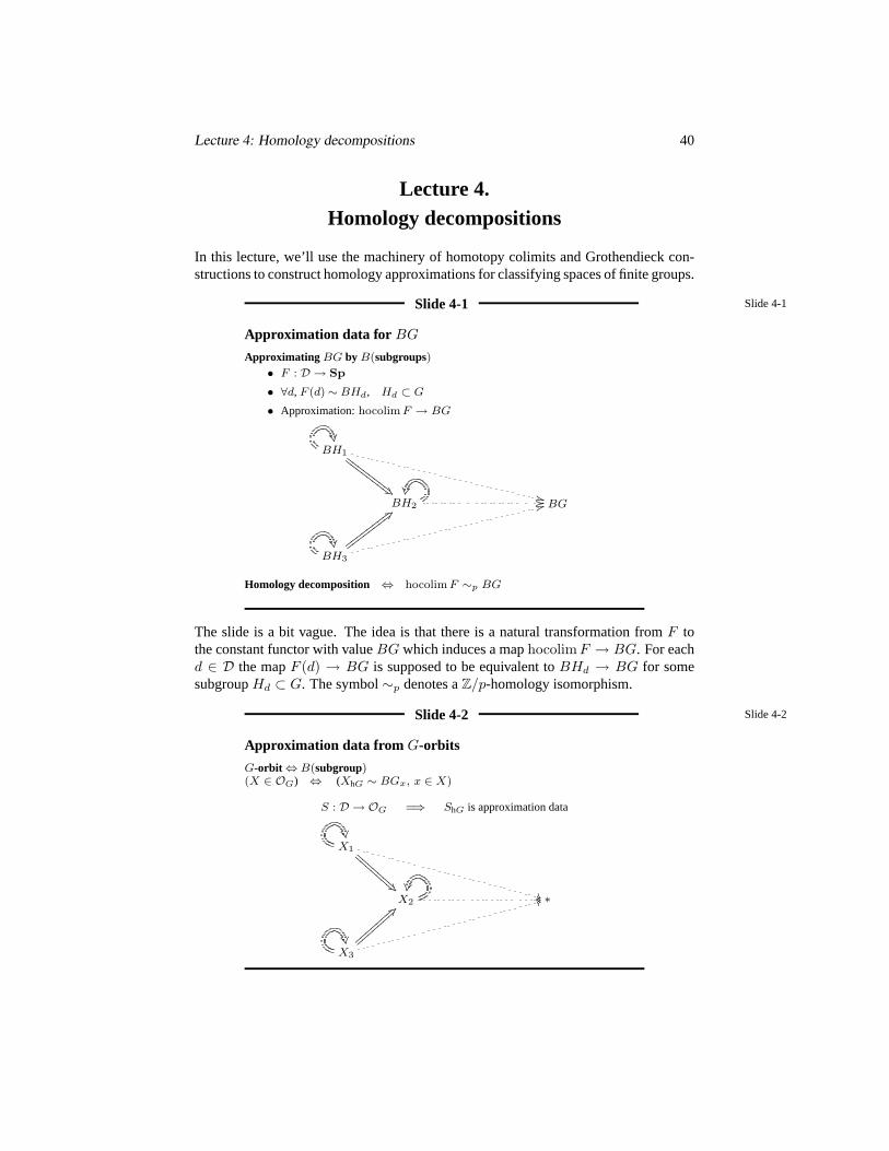
Approximating BG by B(subgroups)• F : D → Sp
• ∀d, F (d) ∼ BHd, Hd ⊂ G
• Approximation:hocolim F → BG
BH1
'GGGG
GGGG
GGGG
GGGG
++BH2
// BG
BH3
7?wwwwwwww
wwwwwwww
33
Homology decomposition ⇔ hocolim F ∼p BG
The slide is a bit vague. The idea is that there is a natural transformation fromF tothe constant functor with valueBG which induces a maphocolim F → BG. For eachd ∈ D the mapF (d) → BG is supposed to be equivalent toBHd → BG for somesubgroupHd ⊂ G. The symbol∼p denotes aZ/p-homology isomorphism.
Slide 4-2 Slide 4-2
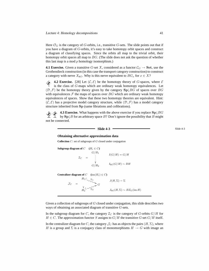
Approximation data from G-orbits
G-orbit ⇔ B(subgroup)(X ∈ OG) ⇔ (XhG ∼ BGx, x ∈ X)
S : D → OG =⇒ ShG is approximation data
X1
%CC
CCCC
C
CCCC
CCC
++X2
// ∗
X3
9A
33
Lecture 4: Homology decompositions 41
HereOG is the category ofG-orbits, i.e., transitiveG-sets. The slide points out that ifyou have a diagram ofG-orbits, it’s easy to take homotopy orbit spaces and constructa diagram of classifying spaces. Since the orbits all map to the trivial orbit, theirhomotopy orbit spaces all map toBG. (The slide does not ask the question of whetherthis last map is a modp homology isomorphism.)
4.1 Exercise.Given a transitiveG-setX, considered as a functorCG → Set, use theGrothendieck construction (in this case the transport category construction) to constructa category with nerveXhG. Why is this nerve equivalent toBGx for x ∈ X?
4.2 Exercise. [28] Let (C, E) be the homotopy theory ofG-spaces, whereEis the class ofG-maps which are ordinary weak homotopy equivalences. Let
(D,F) be the homotopy theory given by the categorySp↓BG of spaces overBGwith equivalencesF the maps of spaces overBG which are ordinary weak homotopyequivalences of spaces. Show that these two homotopy theories are equivalent. Hint:(C, E) has a projective model category structure, while(D,F) has a model categorystructure inherited fromSp (same fibrations and cofibrations).
4.3 Exercise.What happens with the above exercise if you replaceSp↓BGbySp↓B for an arbitrary spaceB? Don’t ignore the possibility thatB might
not be connected.
Slide 4-3 Slide 4-3
Obtaining alternative approximation data
Collection C: set of subgroups ofG closed under conjugation
Subgroup diagram ofC (Hi ∈ C)
IC =
G/H1
G/H2
I(G/H) = G/H
IhG(G/H) ∼ BH
Centralizer diagram of C (im(Hi) ∈ C)
JC =
H1 v
Σ1
)))i)i)i)i
G
H2
( Σ2
555u5u5u5u
J(H, Σ) = Σ
JhG(H, Σ) ∼ BZG(im H)
Given a collection of subgroups ofG closed under conjugation, this slide describes twoways of obtaining an associated diagram of transitiveG-sets.
In the subgroup diagram forC, the categoryIC is the category ofG-orbitsG/H forH ∈ C. The approximation functorS assigns toG/H the transitiveG-setG/H itself.
In the centralizer diagram forC, the categoryJC has as objects the pairs(H,Σ), whereH is a group andΣ is a conjugacy class of monomorphismsH → G with image an
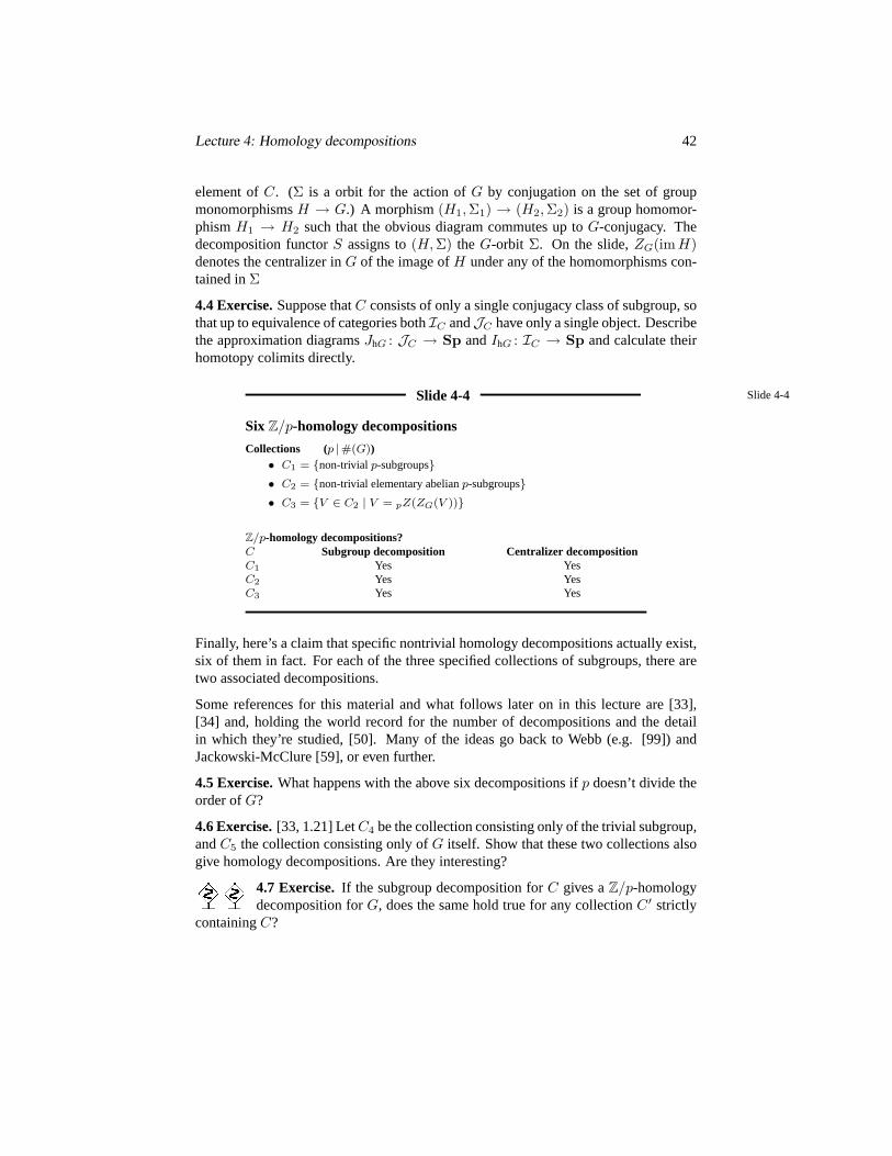
Lecture 4: Homology decompositions 42
element ofC. (Σ is a orbit for the action ofG by conjugation on the set of groupmonomorphismsH → G.) A morphism(H1,Σ1) → (H2,Σ2) is a group homomor-phismH1 → H2 such that the obvious diagram commutes up toG-conjugacy. Thedecomposition functorS assigns to(H,Σ) the G-orbit Σ. On the slide,ZG(im H)denotes the centralizer inG of the image ofH under any of the homomorphisms con-tained inΣ
4.4 Exercise.Suppose thatC consists of only a single conjugacy class of subgroup, sothat up to equivalence of categories bothIC andJC have only a single object. Describethe approximation diagramsJhG : JC → Sp andIhG : IC → Sp and calculate theirhomotopy colimits directly.
Slide 4-4 Slide 4-4
Six Z/p-homology decompositions
Collections (p |#(G))• C1 = non-trivialp-subgroups• C2 = non-trivial elementary abelianp-subgroups• C3 = V ∈ C2 | V = pZ(ZG(V ))
Z/p-homology decompositions?C Subgroup decomposition Centralizer decompositionC1 Yes YesC2 Yes YesC3 Yes Yes
Finally, here’s a claim that specific nontrivial homology decompositions actually exist,six of them in fact. For each of the three specified collections of subgroups, there aretwo associated decompositions.
Some references for this material and what follows later on in this lecture are [33],[34] and, holding the world record for the number of decompositions and the detailin which they’re studied, [50]. Many of the ideas go back to Webb (e.g. [99]) andJackowski-McClure [59], or even further.
4.5 Exercise.What happens with the above six decompositions ifp doesn’t divide theorder ofG?
4.6 Exercise.[33, 1.21] LetC4 be the collection consisting only of the trivial subgroup,andC5 the collection consisting only ofG itself. Show that these two collections alsogive homology decompositions. Are they interesting?
4.7 Exercise.If the subgroup decomposition forC gives aZ/p-homologydecomposition forG, does the same hold true for any collectionC ′ strictly
containingC?
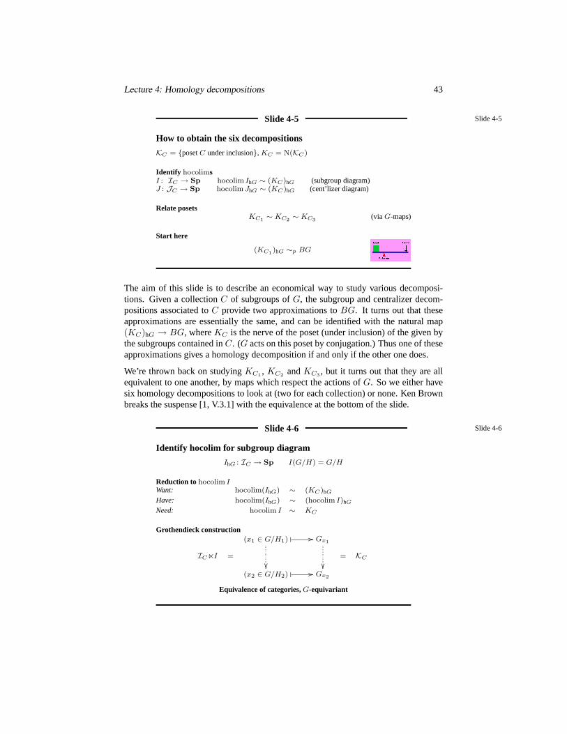
Lecture 4: Homology decompositions 43
Slide 4-5 Slide 4-5
How to obtain the six decompositions
KC = posetC under inclusion, KC = N(KC)
Identify hocolimsI : IC → Sp hocolim IhG ∼ (KC)hG (subgroup diagram)J : JC → Sp hocolim JhG ∼ (KC)hG (cent’lizer diagram)
Relate posetsKC1 ∼ KC2 ∼ KC3 (via G-maps)
Start here
(KC1 )hG ∼p BG
The aim of this slide is to describe an economical way to study various decomposi-tions. Given a collectionC of subgroups ofG, the subgroup and centralizer decom-positions associated toC provide two approximations toBG. It turns out that theseapproximations are essentially the same, and can be identified with the natural map(KC)hG → BG, whereKC is the nerve of the poset (under inclusion) of the given bythe subgroups contained inC. (G acts on this poset by conjugation.) Thus one of theseapproximations gives a homology decomposition if and only if the other one does.
We’re thrown back on studyingKC1 , KC2 andKC3 , but it turns out that they are allequivalent to one another, by maps which respect the actions ofG. So we either havesix homology decompositions to look at (two for each collection) or none. Ken Brownbreaks the suspense [1, V.3.1] with the equivalence at the bottom of the slide.
Slide 4-6 Slide 4-6
Identify hocolim for subgroup diagram
IhG : IC → Sp I(G/H) = G/H
Reduction tohocolim IWant: hocolim(IhG) ∼ (KC)hG
Have: hocolim(IhG) ∼ (hocolim I)hG
Need: hocolim I ∼ KC
Grothendieck construction
ICnI =
(x1 ∈ G/H1)
// Gx1
(x2 ∈ G/H2)
// Gx2
= KC
Equivalence of categories,G-equivariant
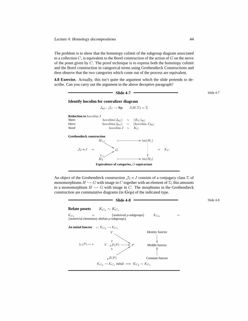
Lecture 4: Homology decompositions 44
The problem is to show that the homotopy colimit of the subgroup diagram associatedto a collectionC, is equivalent to the Borel construction of the action ofG on the nerveof the poset given byC. The proof technique is to express both the homotopy colimitand the Borel construction in categorical terms using Grothendieck Constructions andthen observe that the two categories which come out of the process are equivalent.
4.8 Exercise. Actually, this isn’t quite the argument which the slide pretends to de-scribe. Can you carry out the argument in the above deceptive paragraph?
Slide 4-7 Slide 4-7
Identify hocolim for centralizer diagram
JhG : JC → Sp J(H, Σ) = Σ
Reduction tohocolim JWant: hocolim(JhG) ∼ (KC)hG
Have: hocolim(JhG) ∼ (hocolim J)hG
Need: hocolim J ∼ KC
Grothendieck construction
JCnJ =
H1 s
&&LLLLLL
// im(H1)
G
H2
+
88rrrrrr // im(H2)
= KC
Equivalence of categories,G-equivariant
An object of the Grothendieck constructionJCnJ consists of a conjugacy classΣ ofmonomorphismsH → G with image inC together with an element ofΣ; this amountsto a monomorphismH → G with image inC. The morphisms in the Grothendieckconstruction are commutative diagrams (inGrp) of the indicated type.
Slide 4-8 Slide 4-8
Relate posets KC2 ∼ KC1
KC1 = nontrivialp-subgroups KC2 =nontrivial elementary abelianp-subgroups
An initial functor ι : KC2 → KC1
(ι↓P ) ∼ ∗
V
%%KKKKKKKKKK
Identity functor
V · pZ(P ) // P Middle functor
pZ(P )
99sssssssss
OO
Constant functor
OO
KC2 → KC1 initial =⇒ KC2 ∼ KC1
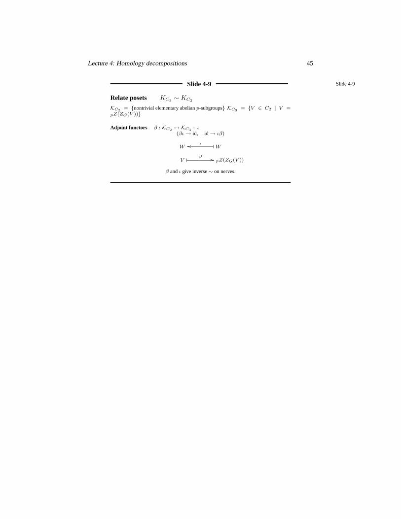
Lecture 4: Homology decompositions 45
Slide 4-9 Slide 4-9
Relate posets KC3 ∼ KC2
KC2 = nontrivial elementary abelianp-subgroups KC3 = V ∈ C2 | V =pZ(ZG(V ))
Adjoint functors β : KC2 ↔ KC3 : ι(βι→ id, id→ ιβ)
W Wιoo
V β // pZ(ZG(V ))
β andι give inverse∼ on nerves.
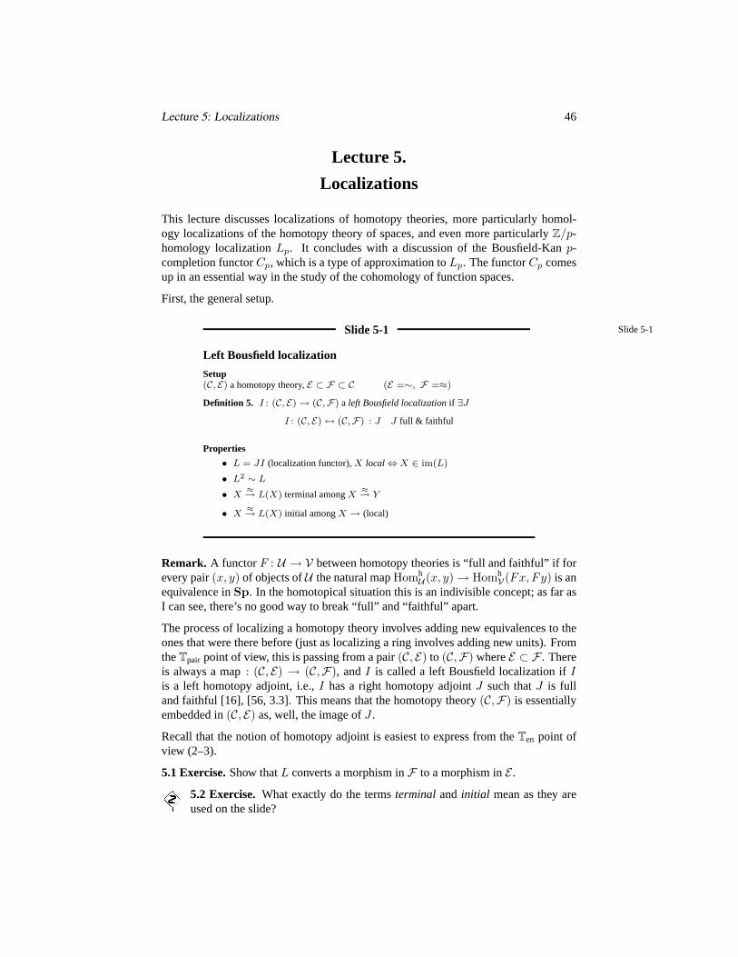
Lecture 5: Localizations 46
Lecture 5.
Localizations
This lecture discusses localizations of homotopy theories, more particularly homol-ogy localizations of the homotopy theory of spaces, and even more particularlyZ/p-homology localizationLp. It concludes with a discussion of the Bousfield-Kanp-completion functorCp, which is a type of approximation toLp. The functorCp comesup in an essential way in the study of the cohomology of function spaces.
First, the general setup.
Slide 5-1 Slide 5-1
Left Bousfield localization
Setup(C, E) a homotopy theory,E ⊂ F ⊂ C (E =∼, F =≈)
Definition 5. I : (C, E)→ (C,F) a left Bousfield localizationif ∃J
I : (C, E)↔ (C,F) : J J full & faithful
Properties
• L = JI (localization functor),X local⇔X ∈ im(L)
• L2 ∼ L
• X≈→ L(X) terminal amongX
≈→ Y
• X≈→ L(X) initial amongX → (local)
Remark. A functorF : U → V between homotopy theories is “full and faithful” if forevery pair(x, y) of objects ofU the natural mapHomh
U (x, y)→ HomhV(Fx, Fy) is an
equivalence inSp. In the homotopical situation this is an indivisible concept; as far asI can see, there’s no good way to break “full” and “faithful” apart.
The process of localizing a homotopy theory involves adding new equivalences to theones that were there before (just as localizing a ring involves adding new units). FromtheTpair point of view, this is passing from a pair(C, E) to (C,F) whereE ⊂ F . Thereis always a map: (C, E) → (C,F), andI is called a left Bousfield localization ifIis a left homotopy adjoint, i.e.,I has a right homotopy adjointJ such thatJ is fulland faithful [16], [56, 3.3]. This means that the homotopy theory(C,F) is essentiallyembedded in(C, E) as, well, the image ofJ .
Recall that the notion of homotopy adjoint is easiest to express from theTen point ofview (2–3).
5.1 Exercise.Show thatL converts a morphism inF to a morphism inE .
5.2 Exercise.What exactly do the termsterminal and initial mean as they areused on the slide?

Lecture 5: Localizations 47
Slide 5-2 Slide 5-2
Example with discrete categories
Context
• C = Ab
• R = Z[1/p]
• E = (isos),F = f | R⊗ f an iso• (C, E) ∼ModZ, (C,F) ∼ModR
Properties
• L = R⊗ (−), X local⇔X anR-module
• L2 ∼ L
• X≈→ L(X) terminal amongX
≈→ Y
• X≈→ L(X) initial amongX → (local)
This is in fact a legitimate example: the homotopy theory(ModZ,F) is equivalentto the discrete categoryModR. Usually the process of inverting morphisms createshigher homotopy groups in the morphism spacesHomh
C,F (−,−), but not in this case[36, 7.3].
Slide 5-3 Slide 5-3
Another model category dividendE ⊂ F ⊂ CDefinition (f a morphism of C, X an object)• f ⊥ X if Homh
(C,E)(f, X) is an equivalence inSp.
• f< = g : f ⊥ X =⇒ g ⊥ X.
Assume
• (C, E) is a model category++
• there is a mapf such thatF = f<
Theorem
1. (C, E)→ (C,F) is a left Bousfield localization.
2. (C,F) is a model category withCcF = Cc
E .
3. L is the fibrant replacement functor in(C,F).
This slide describes a common situation in which it’s possible to construct and identifya left Bousfield localization. (Maybe [24] it’s theonly situation!) Say that a mapf looks invisible to an objectX in a model category(C, E) (or X can’t seef ) ifHomh(f,X) is an equivalence. The idea is to start with a mapf and letF = f<
be the class of all maps which look look invisible to all spaces which can’t seef .
Lecture 5: Localizations 48
Then, under relatively mild conditions (the++), (C, E) → (C,F) is a left Bousfieldlocalization [56, ch.4] [48].
This is calledlocalization with respect to the mapf . Under the relatively mild con-ditions mentioned above, it turns out that the class of newly inverted mapsf< is (upto E) the class of maps which can be built fromf by homotopy colimit constructions.(This is not quite true: one direction is OK [56, 4.2.9] but the other one is bogus [56,2.1.6]. But it’s not far off.)
5.3 Exercise.Show that the localization on slide 5–2 is localization with respect to themapZ→ Z given by multiplication byp.
5.4 Exercise.Show that in the above situation an objectX is local (i.e.L(X) ∼ X) ifand only iff ⊥ X. (Recall that iff ⊥ X theng ⊥ X for all g ∈ F .) Conclude thatthe class of local objects is closed under homotopy limits.
Slide 5-4 Slide 5-4
Examples of model category localizations (I)
Localization with respect to a mapPick your favorite mapf and letF = f<
C = Sp, f = (Sn+1 → ∗)• f< = g : πi(g) iso for i ≤ n• L = Pn (n’th Postnikov stage)
• (local)= (πi vanishes fori > n)
C = ChZ, f = ⊕i(ΣiZ[1/p]→ 0)
• f< = g : Z/p⊗h g is an equivalence• L = derivedp-completion
• (local)= homology groups are Ext-p-complete
Remark. An abelian groupA is Ext-p-complete[18, VI] [51] if the natural mapA →ExtZ(Z/p∞, A) is an isomorphism. Here “the natural map” is the map induced by theconnecting homomorphism in the exact sequence
0→ Z→ Z[1/p]→ Z/p∞ → 0 .
5.5 Exercise.Show that ifA is a finitely generated abelian group, thenExtZ(Z/p∞, A)is isomorphic to thep-completionAp = lim A/pnA, and thatAp is Ext-p-complete.
5.6 Exercise. Show thatA 7→ ExtZ(Z/p∞, A) is the zero’th left derivedfunctor (in the classical sense of Cartan and Eilenberg) of the functorA 7→
Ap on the category of abelian groups [18, VI.2]. This is an unusual situation in whichit turns out to be interesting to take the left derived functors of a functor which itselfis not left exact, so the zero’th left derived functor does not coincide with the originalfunctor. What’s the first left derived functor in this case?
Lecture 5: Localizations 49
Slide 5-5 Slide 5-5
Examples of model category localizations (II)
Localization with respect to a homology theoryE∗Pick your favoriteE∗, letF = E∗-isos, and follow Bousfield.
Theorem (Bousfield)There exists a magic morphismf with f< = F .
Widely applicable• Spaces
• Spectra
• ChR (e.g,E∗(X) = H∗(A⊗hR X))
• simplicial universal algebras
The original references for localization with respect to homology are [12] (for the spacecase) and [13] (for the spectrum case). It’s worth thinking about the construction of themagic morphismf and about why the construction works; the lemma to look for is [12,11.2] or [49, X.2.8]. Don’t make the mistake of thinking that the mapf is necessarilysubject to human comprehension. For instance, ifE∗ = H∗(; Z/p), the f can betaken to be the coproduct of all monomorphicHZ/p∗-equivalences between countablesimplicial sets (actually, for set theoretic reasons, in forming the coproduct that givesfyou would only take one representative from eachisomorphism classof monomorphicHZ/p∗-equivalence).
5.7 Exercise. Show that a spaceX is local with respect toE∗ (i.e. L(X) ∼ X) ifand only if anyE∗-isomorphismA → B induces an equivalenceHomh(B,X) →Homh(A,X) (cf. 5.4).
Slide 5-6 Slide 5-6
Localization with respect toR-homology,R ⊂ QPropertiesLR = localization inSp with respect toH∗(−; R)
• LR preserves components, connectivity, nilpotency.
• X 1-connected=⇒ πiLR(X) ∼= R⊗ πi(X)
• X 1-connected=⇒ Hi(LRX; Z) ∼= R⊗Hi(X; Z)
• LR preserves fibrations of connected nilpotent spaces.
Algebraization if R = QSp1 = 1-connected spaces, F = H∗(−; Q) isosLie0 = 0-connected DG Lie alg/Q, H = H∗ isos. (Sp1,F) ∼ (Lie0,H)
Lecture 5: Localizations 50
If R ⊂ Q, localization with respect toR-homology is relatively simple, at least for1-connected spaces. The statement that the homotopy theory of simply-connected ra-tional spaces is equivalent to the homotopy theory of connected differential graded Liealgebras overQ is due to Quillen [83]; this was one of the first applications of modelcategory machinery. Sullivan came up with a dual approach [96] that works in thefinite-type case and includes the theory of minimal models (see also [17]). See [55] foran up-to-date survey of rational homotopy theory.
5.8 Exercise.Prove that any simply-connected spaceX is HZ-local, i.e.,LZX ∼ X.
5.9 Exercise.As remarked above, homology localization can also be done in thecategory of spectra [13]. Give an example of a nontrivial spectrumX such that
LZX ∼ ∗.
A connected spaceX is nilpotentif π1(X) is a nilpotent group and, for eachi ≥ 2 thenatural action ofπ1(X) on πi(X) is nilpotent (= trivial up to a finite filtration or inloose terms “upper triangular”).
? 5.10 Exercise.Show that a connected spaceX is nilpotent if and only ifπ1(X)is a nilpotent group and for eachi ≥ 2 the natural action ofπ1(X) on Hi(X; Z) isnilpotent. (HereX is the universal cover ofX, and the action is induced by coveringtransformations.)
? 5.11 Exercise. Show that a connected spaceX is nilpotent if and only if eachPostnikov stage ofX can be built from Eilenberg-Mac Lane spaces by a finite numberof principal fibrations with connected fibre.
5.12 Exercise.Is “connected” necessary in the previous exercise?
Slide 5-7 Slide 5-7
Localization with respect toZ/p-homology
Properties (Completion?)Lp = localization inSp with respect toH∗(−; Z/p)
• Lp preserves components, connectivity, nilpotency.
• X 1-connected, fin. type=⇒ πiLp(X) ∼= Zp ⊗ πi(X)
• X 1-connected=⇒ Hi(LpX; Z) ∼= ??
• Lp preserves fibrations of connected nilpotent spaces.
General formula for homotopy groups ofLpXX 1-connected=⇒
0→ Hom(Z/p∞, πi−1X)→ πiLpX → Ext(Z/p∞, πiX)→ 0
The slide points out that from the point of view of the homotopy groups, localizing a1-connected space with respect toHZ/p looks like a type of completion.

Lecture 5: Localizations 51
? 5.13 Exercise.Verify that the description on the slide of theHZ/p-localization ofa 1-connected spaceX of finite type is correct. One approach is to calculate the lo-calization of an Eilenberg-MacLane space directly, and then use the fact that the classof HZ/p-local spaces is closed under homotopy limits, together with various homol-ogy arguments, to climb up the Postnikov tower ofX. (Note that in order to computethe localization of a spaceY , it’s enough to produce a local spaceY ′ and anHZ/p-equivalenceY → Y ′.) Start by showing thatK(Z/p, n) is local with respect toHZ/p(5.4). . Extend this top-GEMs (i.e., products ofK(Z/p.n)’s for variousn, also knownas modp Generalized Eilenberg-Mac Lane spaces) Using homotopy limit arguments(pullback, towers) show that (products of)K(Z/pj , n) andK(Zp, n) (variousj, n) arealsoHZ/p-local. Show thatK(Z, n) → K(Zp, n) gives an isomorphism onHZ/p,and conclude that this is a localization map. Now go Postnikov.
5.14 Exercise.Show that ifX is one-connected, thenLp(LQ(X)) ∼ ∗. What aboutLQ(Lp(X))?
? 5.15 Exercise.The short exact sequence
0→ Z→ Z[1/p]→ Z/p∞ → 0
leads to a fibration sequence
BZ/p∞ → K(Z, 2)→ K(Z[1/p], 2)
Use this or any other technique to show that the mapBZ/p∞ → K(Z, 2) is anHZ/p-equivalence, and so induces an equivalenceLp(BZ/p∞)→ K(Zp, 2) ∼ Lp(BS1).
5.16 Exercise.ComputeH∗(BZ/p∞; Z) andH∗(BZ/p∞; Q). How can thisbe? It’s enough to make a person reread [93, 5.4] with a big cup of coffee.
5.17 Exercise.If A is any direct sum of copies ofZ, show thatK(Ap, n)is HZ/p-local (5.5). Be careful. Calculate thatK(A,n) → K(Ap, n) is an
HZ/p-isomorphism, and conclude that this map is anHZ/p-localization map. Usingvarious Postnikov and fibration arguments in conjunction with 5.6, derive the shortexact sequence at the bottom of the last slide.
Slide 5-8 Slide 5-8
Mixing LQ(X) with the Lp(X)’s to recoverX
The Arithmetic Square (Sullivan)X nilpotent =⇒ homotopy fibre square
X //
Qp Lp(X)
LQX // LQ(
Qp Lp(X))
Lecture 5: Localizations 52
? 5.18 Exercise. If X is 1-connected, use a direct homology calculation to showthat the arithmetic square is a homotopy fibre square. The right vertical map is anHQ-equivalence, and the lower horizontal map is anHZ/p-equivalence (5.14). LetP be the homotopy pullback of the square. Argue thatP maps toLQ(X) by anHQ-equivalence, and that for any primeq the mapP →
∏p Lp(X) is anHZ/q-
equivalence. Observe that for anyq the projection∏
p Lp(X) → Lq(X) is anHZ/q-equivalence (tricky!). Conclude thatX → P induces an isomorphism on integralhomology, and finish the argument by using the fact that both spaces areHZ-local(5.8).
5.19 Exercise.The trickiness mentioned above is relatively minor and hasto do with avoiding the temptation to invoke an imaginary infinite Kunneth
formula. Find an example of a sequence of spacesXn such that eachXn has, say,the rational cohomology of a point, but
∏n Xn does not. How about an example with
integral homology?
5.20 Exercise.LetA andB be sets of primes, and writeLA, for instance, forLZ[p−1:p∈A].Show that ifX is 1-connected there is a homotopy fibre square
LA∩B(X) //
LA(X)
LB(X) // LA∪B(X)
Many people have studied a number of problems of the following type (under the gen-eral heading of genus problems): given a spaceX, how many spacesY are there (upto equivalence) with the property thatLQY ∼ LQX andLp(Y ) ∼ Lp(X) for all p.If such aY exists, call it aremixingof X, since it’s obtained by takingX apart intop-complete and rational pieces, and then mixing them together in some way.
5.21 Exercise.Let X be a sphere. Produce a remixing ofX not equivalent toX.
(Cheap trick?) Most of the time, ifX has finitely generated integral homology groupsthe interesting remixings ofX are those which also have finitely generated integralhomology. Call these theniceremixings.
5.22 Exercise.Let X be a sphere. Show that any nice remixing ofX is equivalentto X.
5.23 Exercise.Can you produce a 2-cell complex with a nontrivial nice remix-ing?
5.24 Exercise.In theory, all remixings ofX can be constructed by takingthe maps
∏p Lp(X) → LQ(
∏p Lp(X)) andLQ(X) → LQ(
∏p Lp(X))
in the arithmetic square forX and adjusting them. What adjustments are possible?Which adjustments give nice remixings? See [101] for a proof that a finite1-connectedcomplex has only a finite number of homotopically distinct nice remixings.

Lecture 5: Localizations 53
Slide 5-9 Slide 5-9
An approximation to Lp
HZ/p-localization functor Lp
HZ/p-local
spaces
J
I //
HZ/p-local
spaces
spaces
RKanhJ (I)∼Lp
99rrrrrrrrrr
Bousfield-Kanp-completion functor Cp (Lp → Cp) p-GEMs
j
i //
HZ/p-local
spaces
spaces
RKanhj(i)∼Cp
99rrrrrrrrrr
Recall that ap-GEM is a product of copies ofK(Z/p, n)’s for variousn. The categoryof p-GEMs is to be taken as a full subcategory of spaces.
The fact thatRKanhJ(I) ∼ Lp follows from the fact that homotopy Kan extensions
can be computed pointwise (cf. 2.3 and 2.23) and the fact that for any spaceX, X↓JhasX → Lp(X) has a (homotopically) initial object (slide 5–1). The functorCp,denoted(Z/p)∞ in [18], is defined by an explicit cosimplicial construction [18, I.4];the expression as a homotopy right Kan extension is from [18, XI.10.6].
5.25 Exercise.(This is probably very hard, or impossible.) For functorsF :C → D andX : C → Sp, observe that the right homotopy Kan extension
RKanhF (X) can be computed by the formula
RKanhF (X)(d) ∼ Homh
SpC (c 7→ HomhD(d, c), X) .
(This is the formula for the right homotopy Kan extension from slide 3–7.) Now for anyspaceX, let K(X) be the functor onp-GEMs given byA 7→ Homh(X, A). This is akind of cochain functor; the homotopy groups ofHomh(X, A) are various cohomologygroups ofX with coefficients in the homotopy groups ofA (in other words, variousproducts of modp cohomology groups ofX). Applied to the case ofCp, the aboveformula states thatCp(X) is the space of natural maps, asA ranges throughp-GEMs,of K(X, A) to A. In other words,Cp(X) is some sort of double-dual ofX over thecategory ofp-GEMs. The problem is to find some interesting relationship betweenthis remark and Mandell’s theorem [69] that (under certain finiteness and nilpotencyassumptions)Cp(X) is the space ofE∞ Fp-algebra maps fromC∗(X, Fp) to Fp.
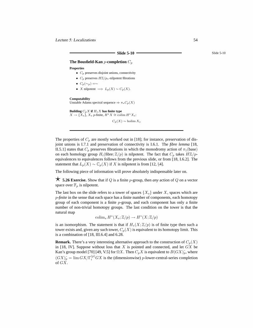
Lecture 5: Localizations 54
Slide 5-10 Slide 5-10
The Bousfield-Kanp-completionCp
Properties• Cp preserves disjoint unions, connectivity
• Cp preservesHZ/p∗-nilpotent fibrations
• Cp(∼p) =∼• X nilpotent =⇒ Lp(X) ∼ Cp(X).
ComputabilityUnstable Adams spectral sequence⇒ π∗Cp(X)
Building CpX if H∗X has finite typeX → Xs, Xs p-finite, H∗X ∼= colim H∗Xs:
Cp(X) ∼ holim Xs
The properties ofCp are mostly worked out in [18]; for instance, preservation of dis-joint unions is I.7.1 and preservation of connectivity is I.6.1. Thefibre lemma[18,II.5.1] states thatCp preserves fibrations in which the monodromy action ofπ1(base)on each homology groupHi(fibre; Z/p) is nilpotent. The fact thatCp takesHZ/p-equivalences to equivalences follows from the previous slide, or from [18, I.6.2]. Thestatement thatLp(X) ∼ Cp(X) if X is nilpotent is from [12,§4].
The following piece of information will prove absolutely indispensable later on.
? 5.26 Exercise.Show that ifQ is a finitep-group, thenanyaction ofQ on a vectorspace overFp is nilpotent.
The last box on the slide refers to a tower of spacesXs underX, spaces which arep-finite in the sense that each space has a finite number of components, each homotopygroup of each component is a finitep-group, and each component has only a finitenumber of non-trivial homotopy groups. The last condition on the tower is that thenatural map
colims H∗(Xs; Z/p)→ H∗(X; Z/p)
is an isomorphism. The statement is that ifH∗(X; Z/p) is of finite type then such atower exists and, given any such tower,Cp(X) is equivalent to its homotopy limit. Thisis a combination of [18, III.6.4] and 6.28.
Remark. There’s a very interesting alternative approach to the construction ofCp(X)in [18, IV]. Suppose without loss thatX is pointed and connected, and letGX beKan’s group model [70] [49, V.5] forΩX. ThenCpX is equivalent toB(GX)p, where
(GX)p = lim GX/Γ(p)i GX is the (dimensionwise)p-lower-central-series completion
of GX.

Lecture 5: Localizations 55
Slide 5-11 Slide 5-11
The Bousfield-Kanp-completionCp: good & bad
Definition• LpX ∼ CpX = X p-good
• LpX 6∼ CpX = X p-bad
p-good examples
• X nilpotent (e.g.π1X trivial)
• π1X finite
p-bad examples
• S1 ∨ S1
• S1 ∨ Sn
News flashCp(p-badX) sighted in the wild!
The spaceCp(X) is alwaysHZ/p-local (it’s a homotopy limit ofp-GEMs, cf. 5–9),and soCpX ∼ LpX if and only if X → CpX is anHZ/p-equivalence. This last is thedefinition of “Z/p-good” in [18, I.5]. Thep-good examples are from [18]. Bousfield[15] provides the indicatedp-bad examples.
The last statement promises that in the near future we will encounter thep-completionof a p-bad space in a relatively simple geometric setting that doesn’t seem to deservesuch a visitation.
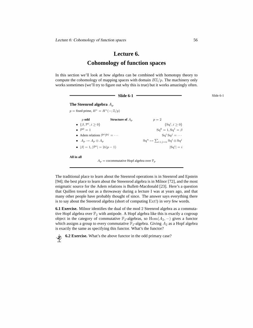
Lecture 6: Cohomology of function spaces 56
Lecture 6.
Cohomology of function spaces
In this section we’ll look at how algebra can be combined with homotopy theory tocompute the cohomology of mapping spaces with domainBZ/p. The machinery onlyworks sometimes (we’ll try to figure out why this is true) but it works amazingly often.
Slide 6-1 Slide 6-1
The Steenrod algebraAp
p = fixed prime,H∗ = H∗(−; Z/p)
p odd Structure of Ap p = 2
• β,Pi, i ≥ 0 Sqi, i ≥ 0• P0 = 1 Sq0 = 1, Sq1 = β
• Adem relationsPiPj = · · · Sqi Sqj = · · ·• Ap → Ap ⊗Ap Sqn 7→
Pi+j=n Sqi⊗ Sqj
• |β| = 1, |Pi| = 2i(p− 1) |Sqi| = i
All in allAp = cocommutative Hopf algebra overFp
The traditional place to learn about the Steenrod operations is in Steenrod and Epstein[94]; the best place to learn about the Steeenrod algebra is in Milnor [72], and the mostenigmatic source for the Adem relations is Bullett-Macdonald [23]. Here’s a questionthat Quillen tossed out as a throwaway during a lecture I was at years ago, and thatmany other people have probably thought of since. The answer says everything thereis to say about the Steenrod algebra (short of computingExt!) in veryfew words.
6.1 Exercise.Milnor identifies the dual of the mod2 Steenrod algebra as a commuta-tive Hopf algebra overF2 with antipode. A Hopf algebra like this is exactly a cogroupobject in the category of commutativeF2-algebras, soHom(A2,−) gives a functorwhich assigns a group to every commutativeF2-algebra. GivingA2 as a Hopf algebrais exactly the same as specifying this functor. What’s the functor?
6.2 Exercise.What’s the above functor in the odd primary case?

Lecture 6: Cohomology of function spaces 57
Slide 6-2 Slide 6-2
Modules and algebras overAp
Modules overAp
• Gradedmodules Sqi : Mk →Mk+i
• U = unstable modules Sqi x = 0, i > |x|• M , N (unstable) modules=⇒ M ⊗N (unstable) module
Algebra over Ap
• Graded algebras,µ : M ⊗M →M respectsAp
• K = unstable algebras Sq|x| x = x2
• R, S (unstable) algebras=⇒ R⊗ S (unstable) algebra
Geometry
• H∗(suspension spectrum) ∈ U• H∗(space) ∈ K
The slide glosses over the fact thatK is the category of unstablegraded-commutativealgebras overAp.
6.3 Exercise. What kind of geometric object would give rise to an algebra overAp
which isnot unstable?
6.4 Exercise.Give an example of an object ofK which is not isomorphic toH∗X forany spaceX.
6.5 Exercise. Why are objects inK andU necessarily concentrated in non-negativedegrees?
Slide 6-3 Slide 6-3
The functor T
V = V1 = Z/p, H = H∗BV
Left adjoint(s) to H⊗−TU : U ↔ U : (H⊗−)
TU = TK (= T ) TK : K ↔ K : (H⊗−)
KTK
//
forget
K
forget
U
TU // U
Crucial properties• T is exact
• T preserves⊗• Same properties withV1 ↔ Vn = (Z/p)n
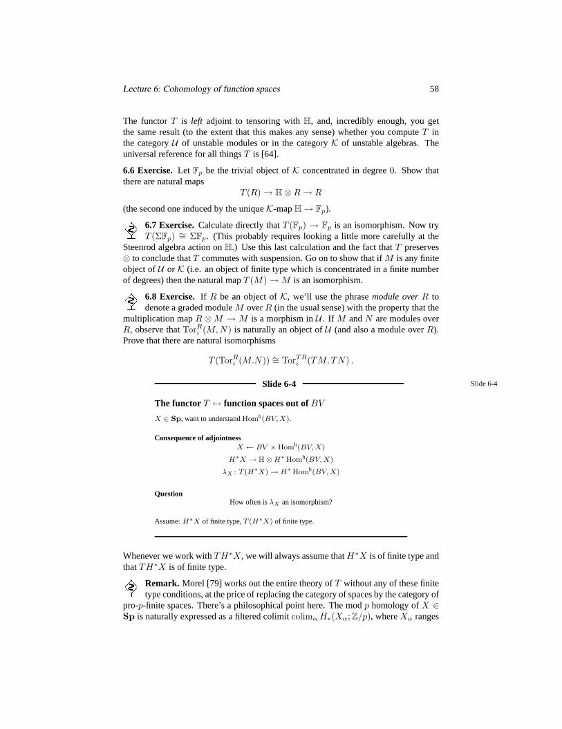
Lecture 6: Cohomology of function spaces 58
The functorT is left adjoint to tensoring withH, and, incredibly enough, you getthe same result (to the extent that this makes any sense) whether you computeT inthe categoryU of unstable modules or in the categoryK of unstable algebras. Theuniversal reference for all thingsT is [64].
6.6 Exercise. Let Fp be the trivial object ofK concentrated in degree0. Show thatthere are natural maps
T (R)→ H⊗R→ R
(the second one induced by the uniqueK-mapH→ Fp).
6.7 Exercise.Calculate directly thatT (Fp) → Fp is an isomorphism. Now tryT (ΣFp) ∼= ΣFp. (This probably requires looking a little more carefully at the
Steenrod algebra action onH.) Use this last calculation and the fact thatT preserves⊗ to conclude thatT commutes with suspension. Go on to show that ifM is any finiteobject ofU orK (i.e. an object of finite type which is concentrated in a finite numberof degrees) then the natural mapT (M)→M is an isomorphism.
6.8 Exercise. If R be an object ofK, we’ll use the phrasemodule overR todenote a graded moduleM overR (in the usual sense) with the property that the
multiplication mapR ⊗M → M is a morphism inU . If M andN are modules overR, observe thatTorR
i (M,N) is naturally an object ofU (and also a module overR).Prove that there are natural isomorphisms
T (TorRi (M.N)) ∼= TorTR
i (TM,TN) .
Slide 6-4 Slide 6-4
The functor T ↔ function spaces out ofBV
X ∈ Sp, want to understandHomh(BV, X).
Consequence of adjointnessX ← BV ×Homh(BV, X)
H∗X → H⊗H∗ Homh(BV, X)
λX : T (H∗X)→ H∗ Homh(BV, X)
QuestionHow often isλX an isomorphism?
Assume:H∗X of finite type,T (H∗X) of finite type.
Whenever we work withTH∗X, we will always assume thatH∗X is of finite type andthatTH∗X is of finite type.
Remark. Morel [79] works out the entire theory ofT without any of these finitetype conditions, at the price of replacing the category of spaces by the category of
pro-p-finite spaces. There’s a philosophical point here. The modp homology ofX ∈Sp is naturally expressed as a filtered colimitcolimα H∗(Xα; Z/p), whereXα ranges
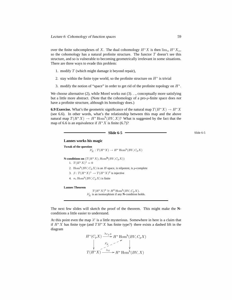
Lecture 6: Cohomology of function spaces 59
over the finite subcomplexes ofX. The dual cohomologyH∗X is thenlimα H∗Xα,so the cohomology has a natural profinite structure. The functorT doesn’t see thisstructure, and so is vulnerable to becoming geometrically irrelevant in some situations.There are three ways to evade this problem:
1. modify T (which might damage it beyond repair),
2. stay within the finite type world, so the profinite structure onH∗ is trivial
3. modify the notion of “space” in order to get rid of the profinite topology onH∗.
We choose alternative (2), while Morel works out (3). . ., conceptually more satisfyingbut a little more abstract. (Note that the cohomology of a pro-p-finite space doesnothave a profinite structure, although its homology does.)
6.9 Exercise.What’s the geometric significance of the natural mapT (H∗X)→ H∗X(see 6.6). In other words, what’s the relationship between this map and the abovenatural mapT (H∗X) → H∗ Homh(BV,X)? What is suggested by the fact that themap of 6.6 is an equivalence ifH∗X is finite (6.7)?
Slide 6-5 Slide 6-5
Lannes works his magic
Tweak of the questionλc
X : T (H∗X)→ H∗ Homh(BV, CpX)
N-conditions on(T (H∗X), Homh(BV, CpX))
1. T (H∗X)1 = 0
2. Homh(BV, CpX) is anH-space, is nilpotent, isp-complete
3. β : T (H∗X)1 → T (H∗X)2 is injective
4. π1 Homh(BV, CpX) is finite
Lannes TheoremT (H∗X)0 ∼= H0 Homh(BV, CpX).
λcX is an isomorphism if anyN-condition holds.
The next few slides will sketch the proof of the theorem. This might make theN-conditions a little easier to understand.
At this point even the mapλc is a little mysterious. Somewhere in here is a claim thatif H∗X has finite type (andTH∗X has finite type?) there exists a dashed lift in thediagram
H∗(CpX)λCpX //
H∗ Homh(BV,CpX)
T (H∗X)
λX //
λcX
66mmmmmmmH∗ Homh(BV, X)

Lecture 6: Cohomology of function spaces 60
It’s probably unclear why anything likeCpX should show up here. One useful remarkis thatH∗X only depends on theZ/p-homology type ofX, and so anything that’sconstructed out ofH∗X, such asTH∗X, can at the very best only give informationaboutLpX. This would explain an appearance ofLpX in the theorem, but there youare, it’sCpX, notLpX. We’ll see what’s going on in a minute.
? 6.10 Exercise.Show that ifX is one-connected, the natural mapκ : Homh(BV,X)→Homh(BV,CpX) induces is aZ/p-homology equivalence. (Show that the homotopyfibre F of X → CpX has uniquelyp-divisible homotopy groups. Argue that the ho-motopy fibre ofκ over a mapf : BV → CpX is the space of sections of a bundleoverBV with fibre F induced fromf . If it helps, interpret this space of sections as ahomotopy fixed point setF hV for an action ofV onF depending onf . Show that thehomotopy groups of such a space of sections (=homotopy fixed point set) are uniquelyp-divisible, and thus (careful withπ1!) that the space isZ/p-acyclic.)
6.11 Exercise.How far beyond1-connected spaces does the above result extend?What happens ifπ1X is finite? What ifX is a connected loop space (careful: the
homotopy fibreF might not be connected)?
6.12 Exercise.The slide is a bit cavalier; produce an example of anH-space whichis not nilpotent. (Presumably, the author of the slide didnot mean to allow this as apossibility.)
6.13 Exercise.Show that the statement aboutT (H∗X)0 is equivalent to the statementthat there is an isomorphism[BV,CpX] ∼= HomK(H∗X, H).
Slide 6-6 Slide 6-6
Outlining the proof
X p-finite ↔• π0X finite
• πiX finite p-group
• πiX = 0 for i >> 0.
One step at a time
1. λX an iso ifX = K(Z/p, n)
2. λX an iso ifX is p-finite
3. A tour of towers
4. λcX exists, iso if anyN-condition holds
We’ll approach the proof in three steps, with a digression on towers of spaces betweenthe second and the third. The line of argument is from [29], augmented by [92].
In the definition ofp-finite, the conditions onπiX are supposed to hold for all possiblechoices of a basepoint inX. A spaceX is p-finite if and only ifX has a finite numberof components and each component isp-finite.
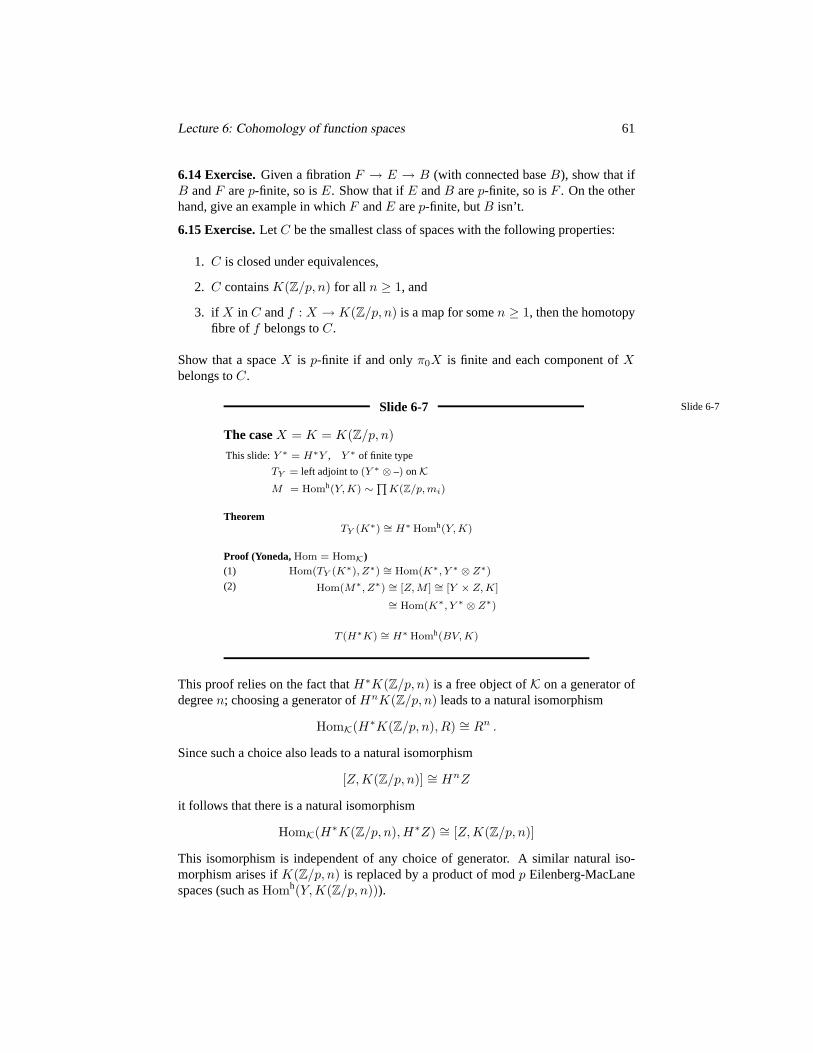
Lecture 6: Cohomology of function spaces 61
6.14 Exercise.Given a fibrationF → E → B (with connected baseB), show that ifB andF arep-finite, so isE. Show that ifE andB arep-finite, so isF . On the otherhand, give an example in whichF andE arep-finite, butB isn’t.
6.15 Exercise.Let C be the smallest class of spaces with the following properties:
1. C is closed under equivalences,
2. C containsK(Z/p, n) for all n ≥ 1, and
3. if X in C andf : X → K(Z/p, n) is a map for somen ≥ 1, then the homotopyfibre off belongs toC.
Show that a spaceX is p-finite if and onlyπ0X is finite and each component ofXbelongs toC.
Slide 6-7 Slide 6-7
The caseX = K = K(Z/p, n)This slide:Y ∗ = H∗Y , Y ∗ of finite type
TY = left adjoint to(Y ∗ ⊗ –) onKM = Homh(Y, K) ∼
QK(Z/p, mi)
TheoremTY (K∗) ∼= H∗ Homh(Y, K)
Proof (Yoneda,Hom = HomK)(1) Hom(TY (K∗), Z∗) ∼= Hom(K∗, Y ∗ ⊗ Z∗)
(2) Hom(M∗, Z∗) ∼= [Z, M ] ∼= [Y × Z, K]
∼= Hom(K∗, Y ∗ ⊗ Z∗)
T (H∗K) ∼= H∗ Homh(BV, K)
This proof relies on the fact thatH∗K(Z/p, n) is a free object ofK on a generator ofdegreen; choosing a generator ofHnK(Z/p, n) leads to a natural isomorphism
HomK(H∗K(Z/p, n), R) ∼= Rn .
Since such a choice also leads to a natural isomorphism
[Z,K(Z/p, n)] ∼= HnZ
it follows that there is a natural isomorphism
HomK(H∗K(Z/p, n),H∗Z) ∼= [Z,K(Z/p, n)]
This isomorphism is independent of any choice of generator. A similar natural iso-morphism arises ifK(Z/p, n) is replaced by a product of modp Eilenberg-MacLanespaces (such asHomh(Y, K(Z/p, n))).

Lecture 6: Cohomology of function spaces 62
6.16 Exercise.Prove that ifY is any space, thenHomh(Y, K(Z/p, n)) is equivalentto a product of modp Eilenberg-MacLane spaces. (This is probably a lot easier in thesimplicial world.)
6.17 Exercise.The application of Yoneda’s lemma above seems to be questionable,because the argument shows only that the two objects in question (TY (K∗) andM∗)represent the same functor on the subcategory ofK given by objectsZ∗ which can berealized as the cohomology of a space. What saves the day?
6.18 Exercise. An argument identical to the one on the slide shows that theLannes map
λX : T (H∗X)→ H∗ Homh(BV, X)
is an equivalence ifX is a finite product of modp Eilenberg-MacLane spaces. Whathappens ifX is an infinite product of such Eilenberg-MacLane spaces? What about ifX is just tall (X =
∏∞i=1K(Z/p, i)) or just wide (X =
∏∞i=1 K(Z/p, n)) ?
Slide 6-8 Slide 6-8
The case in whichX is p-finite.
X → Y → K = K(Z/p, n)
H∗X ⇐ TorH∗K(H∗Y, Fp) EMSSλY an iso (Ex. 6.15)
Mapping side (EMSS+ Homh preserves fibrations)H∗ Homh(BV, X)⇐ TorTH∗K(TH∗Y, Fp)
Space side (T is nice)TH∗X ⇐ TorTH∗K(TH∗Y, Fp)
T (H∗X) ∼= H∗ Homh(BV, X)
The argument with the Eilenberg-Moore spectral sequence is from [29].
The point here is to work by induction on the complexity ofX. By Exercise 6.15 wecan get any connectedp-finite X by starting from a point and repeatedly taking fibresof maps into modp Eilenberg-MacLane spaces.
6.19 Exercise.Why is it clear that ifλZ is an isomorphism for each componentZ ofX, thenλX is an isomorphism?
6.20 Exercise.Suppose thatF → E → B is a fibration and that bothH∗B andH∗Eare of finite type. The modp cohomology Eilenberg-Moore spectral sequence for thisfibration converges strongly (i.e. with finite filtrations in each degree) if and only if themonodromy action ofπ1B on each one of the cohomology groupsHiF is nilpotent(trivial up to a finite filtration). So why does the mapping side spectral sequence on theslide converge?

Lecture 6: Cohomology of function spaces 63
6.21 Exercise.The “T is nice” tag is a little bit too glib. The nice propertiesof T do lead to a formula
TorTH∗K(TH∗Y, Fp) ∼= T
TorH∗K(H∗Y, Fp)
but this a formula in the category of graded objects inU (oneTori for eachi). Follow-ing the spectral sequence through is no problem, sinceT is exact and commutes withcolimits (why?), but there’s some geometric work to be done in the limit in order tostitch the graded pieces together. Figure out what this work is, and explain how to doit. It may help to look at Rector’s paper [87].
Slide 6-9 Slide 6-9
Tower Us = · · · → Un → Un−1 → · · · → U0
colim H∗Us?= H∗ holim Us
Assume: eachUn p-finite, colim H∗Us of finite type
N-conditions on (H∗∞ = colim H∗Us, U∞ = holim Us)
1. H1∞ = 0
2. U∞ is anH-space, is nilpotent, isp-complete
3. β : H1∞ → H2
∞ is injective
4. π1U∞ is finite
Tower TheoremH0∞ ∼= H0U∞, always.
H∗∞ ∼= H∗U∞ if any N-condition holds.
See [92] for general background about towers.
The exercises below are meant to set up some of the machinery that’s used in workingwith towers. They more or less lead to a proof of the above theorem, at least in somecases.N-condition (3) is a list of three successively more general alternatives: eitherU∞ is anH-space, or more generallyU∞ is nilpotent, or even more generallyU∞ isp-complete (here and later on, a spaceX is p-complete ifX ∼ CpX). Shipley [92]proves the tower theorem under the assumption thatU∞ is p-complete.
6.22 Exercise. Prove that if each component ofU∞ has a finite fundamentalgroup, or ifH1
∞ = 0, or if the stated Bockstein injectivity holds, thenU∞ isp-complete. (Hint: Show that if a component ofU∞ has a finite fundamental group,then this group is a finitep-group; show that if the Bockstein injectivity holds then eachcomponent ofU∞ has a finite modp vector space as fundamental group; and show thatif H1
∞ = 0 then each component ofU∞ is simply connected.)
First, there is the general problem of understanding homotopy limits of towers and theirhomotopy groups. Note that it is possible to talk about towers in any categoryC; theseare just functors from the poset of nonpositive integers intoC. A map between towersis a natural transformation of functors.

Lecture 6: Cohomology of function spaces 64
6.23 Exercise. (Homotopy limit of a tower) LetUs be a tower inSp. Show thatholim Us can be computed in either of two ways:
• replaceUs up to equivalence by a tower of fibrations, and take the limit of thisreplacement tower, or
• take the space of tuples(u0, ω0, u1, ω1, . . .), whereui ∈ Ui andωi is a path inUi betweenui and the image ofui+1.
(It’s worth it to try to make simplicial sense of the second description.) Letσ :∏
Us →∏Us be the shift map, which sends(u0, u1, . . .) to (u′0, u
′1, . . .), whereu′i is the image
of ui+1 in Ui. Conclude thatholim Us can be interpreted as the homotopy pullback
holim Us//_____
∏Us
(id,σ)
∏Us
diag // (∏
Us)× (∏
Us)
or as the homotopy equalizer
holim Us//___ ∏
Us
id //
σ//∏
Us
or even as the homotopy fixed point set ofσ acting on∏
Us (i.e., the homotopy fixedpoint set of the action on
∏Us of the free monoid on one generator, where the generator
acts byσ).
If As is a tower of abelian group, the shift mapσ :∏
As →∏
As is defined in thesame way as above. The kernel of(1− σ) :
∏As →
∏As is the limit lim As (check
this); the cokernel is denotedlim1 As.
6.24 Exercise. (Milnor sequences) [49, VI.2.15] Show that ifUs is a tower ofpointed one-connected spaces, there are short exact (Milnor) sequences
0→ lim1 πi+1Us → πi holim Us → limπiUs → 0
Definelim1 for a tower of nonabelian groups in such a way that these sequences canbe extended to handleπ1.
6.25 Exercise.Show that a short exact sequence
0→ As → Bs → Cs → 0
of towers of (abelian) groups leads to a six-term exact sequence
0→ limAs → lim Bs → limCs → lim1 As → lim1 Bs → lim1 Cs → 0 .
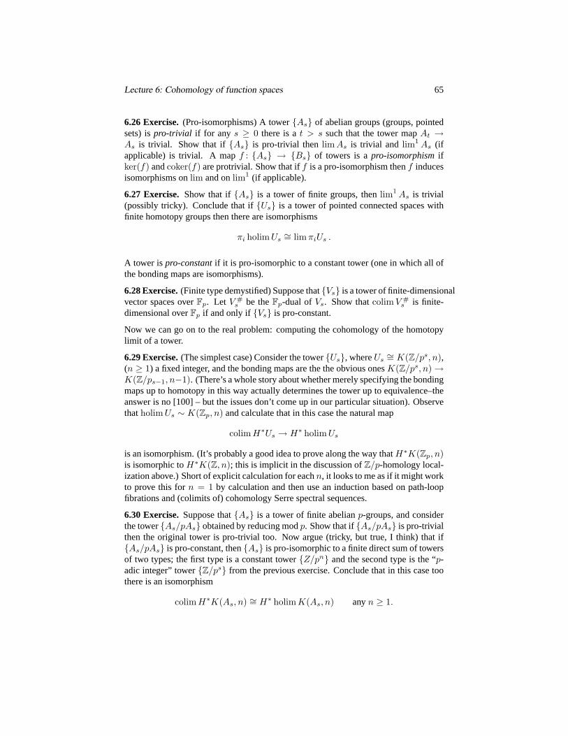
Lecture 6: Cohomology of function spaces 65
6.26 Exercise.(Pro-isomorphisms) A towerAs of abelian groups (groups, pointedsets) ispro-trivial if for any s ≥ 0 there is at > s such that the tower mapAt →As is trivial. Show that ifAs is pro-trivial thenlim As is trivial and lim1 As (ifapplicable) is trivial. A mapf : As → Bs of towers is apro-isomorphismifker(f) andcoker(f) are protrivial. Show that iff is a pro-isomorphism thenf inducesisomorphisms onlim and onlim1 (if applicable).
6.27 Exercise.Show that ifAs is a tower of finite groups, thenlim1 As is trivial(possibly tricky). Conclude that ifUs is a tower of pointed connected spaces withfinite homotopy groups then there are isomorphisms
πi holim Us∼= limπiUs .
A tower ispro-constantif it is pro-isomorphic to a constant tower (one in which all ofthe bonding maps are isomorphisms).
6.28 Exercise.(Finite type demystified) Suppose thatVs is a tower of finite-dimensionalvector spaces overFp. Let V #
s be theFp-dual of Vs. Show thatcolim V #s is finite-
dimensional overFp if and only if Vs is pro-constant.
Now we can go on to the real problem: computing the cohomology of the homotopylimit of a tower.
6.29 Exercise.(The simplest case) Consider the towerUs, whereUs∼= K(Z/ps, n),
(n ≥ 1) a fixed integer, and the bonding maps are the the obvious onesK(Z/ps, n)→K(Z/ps−1, n−1). (There’s a whole story about whether merely specifying the bondingmaps up to homotopy in this way actually determines the tower up to equivalence–theanswer is no [100] – but the issues don’t come up in our particular situation). Observethatholim Us ∼ K(Zp, n) and calculate that in this case the natural map
colim H∗Us → H∗ holim Us
is an isomorphism. (It’s probably a good idea to prove along the way thatH∗K(Zp, n)is isomorphic toH∗K(Z, n); this is implicit in the discussion ofZ/p-homology local-ization above.) Short of explicit calculation for eachn, it looks to me as if it might workto prove this forn = 1 by calculation and then use an induction based on path-loopfibrations and (colimits of) cohomology Serre spectral sequences.
6.30 Exercise.Suppose thatAs is a tower of finite abelianp-groups, and considerthe towerAs/pAs obtained by reducing modp. Show that ifAs/pAs is pro-trivialthen the original tower is pro-trivial too. Now argue (tricky, but true, I think) that ifAs/pAs is pro-constant, thenAs is pro-isomorphic to a finite direct sum of towersof two types; the first type is a constant towerZ/pn and the second type is the “p-adic integer” towerZ/ps from the previous exercise. Conclude that in this case toothere is an isomorphism
colim H∗K(As, n) ∼= H∗ holim K(As, n) anyn ≥ 1.
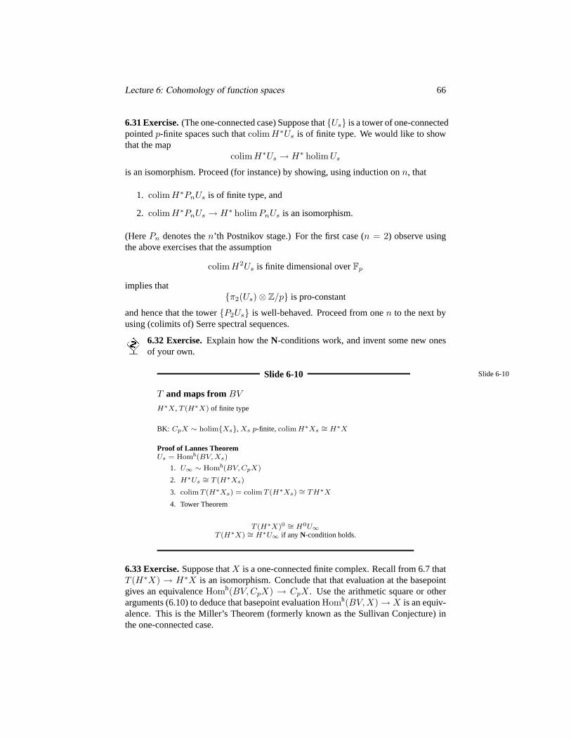
Lecture 6: Cohomology of function spaces 66
6.31 Exercise.(The one-connected case) Suppose thatUs is a tower of one-connectedpointedp-finite spaces such thatcolim H∗Us is of finite type. We would like to showthat the map
colim H∗Us → H∗ holim Us
is an isomorphism. Proceed (for instance) by showing, using induction onn, that
1. colim H∗PnUs is of finite type, and
2. colim H∗PnUs → H∗ holim PnUs is an isomorphism.
(HerePn denotes then’th Postnikov stage.) For the first case (n = 2) observe usingthe above exercises that the assumption
colim H2Us is finite dimensional overFp
implies thatπ2(Us)⊗ Z/p is pro-constant
and hence that the towerP2Us is well-behaved. Proceed from onen to the next byusing (colimits of) Serre spectral sequences.
6.32 Exercise.Explain how theN-conditions work, and invent some new onesof your own.
Slide 6-10 Slide 6-10
T and maps fromBV
H∗X, T (H∗X) of finite type
BK: CpX ∼ holimXs, Xs p-finite, colim H∗Xs∼= H∗X
Proof of Lannes TheoremUs = Homh(BV, Xs)
1. U∞ ∼ Homh(BV, CpX)
2. H∗Us∼= T (H∗Xs)
3. colim T (H∗Xs) = colim T (H∗Xs) ∼= TH∗X
4. Tower Theorem
T (H∗X)0 ∼= H0U∞T (H∗X) ∼= H∗U∞ if any N-condition holds.
6.33 Exercise.Suppose thatX is a one-connected finite complex. Recall from 6.7 thatT (H∗X) → H∗X is an isomorphism. Conclude that that evaluation at the basepointgives an equivalenceHomh(BV,CpX) → CpX. Use the arithmetic square or otherarguments (6.10) to deduce that basepoint evaluationHomh(BV,X)→ X is an equiv-alence. This is the Miller’s Theorem (formerly known as the Sullivan Conjecture) inthe one-connected case.
Lecture 6: Cohomology of function spaces 67
? 6.34 Exercise.Extend the previous exercise to the case in whichBV is replaced byBG for a finitep-groupG. Use induction on the size ofG, the fact that any nontrivialG contains a central element of orderp, and the fact that ifK is a normal subgroup ofGthere is an equivalenceXhG ∼ (XhK)h(G/K). There’s a more general principle here:if X is a space andF → E → B is a fibration sequence over a connected baseB, thenHomh(E,X) can be identified as the space of sections of an associated fibration overB with Homh(F,X) as the fibre. (With some acrobatics, this could be derived fromthe transitivity of homotopy right Kan extensions, but it’s easier to draw a picture.) Ifthe inclusionX → Homh(F,X) of the constant maps is an equivalence, it follows thatHomh(B,X) → Homh(E,X) is also an equivalence. This is another way to look atthe inductive step above.
6.35 Exercise.What are the obstacles to extending the previous exercise to thecase in whichG is an arbitrary finite group? Do homology decompositions help?
Slide 6-11 Slide 6-11
In the presence of a volunteer. . .
Tower version Us as beforeV-condition: ∃Y → Ux inducingH∗Y ∼= colim H∗Us.
Theorem: holim Us ∼ CpY
T -version H∗X, T (H∗X) as beforeV-condition: ∃BV × Y → X inducingH∗Y ∼= T (H∗X).
Theorem: Homh(BV, CpX) ∼ CpY
Y is a (cohomological)volunteer.
This slide describes an assumption very different from theN-conditions under whichit is possible to useT to compute something about a function space. Suppose thereis a homological “volunteer” for the function complex, in the sense there is a spaceYtogether with a map
BV × Y → X (i.e.,Y → Homh(BV,X))
which induces an isomorphism
H∗Y∼=← T (H∗X)
(We’re still assuming thatH∗X is of finite type and thatTH∗X is of finite type.)Then the discussion after slide 5–10, in conjunction with the tower machinery above,produces an equivalenceCpY ∼ Homh(BV,CpX). Note that in this case there isno claim thatT (H∗X) ∼= H∗ Homh(BV,CpX); whether or not this is true dependsentirely on whether or notY is p-good (5–11).
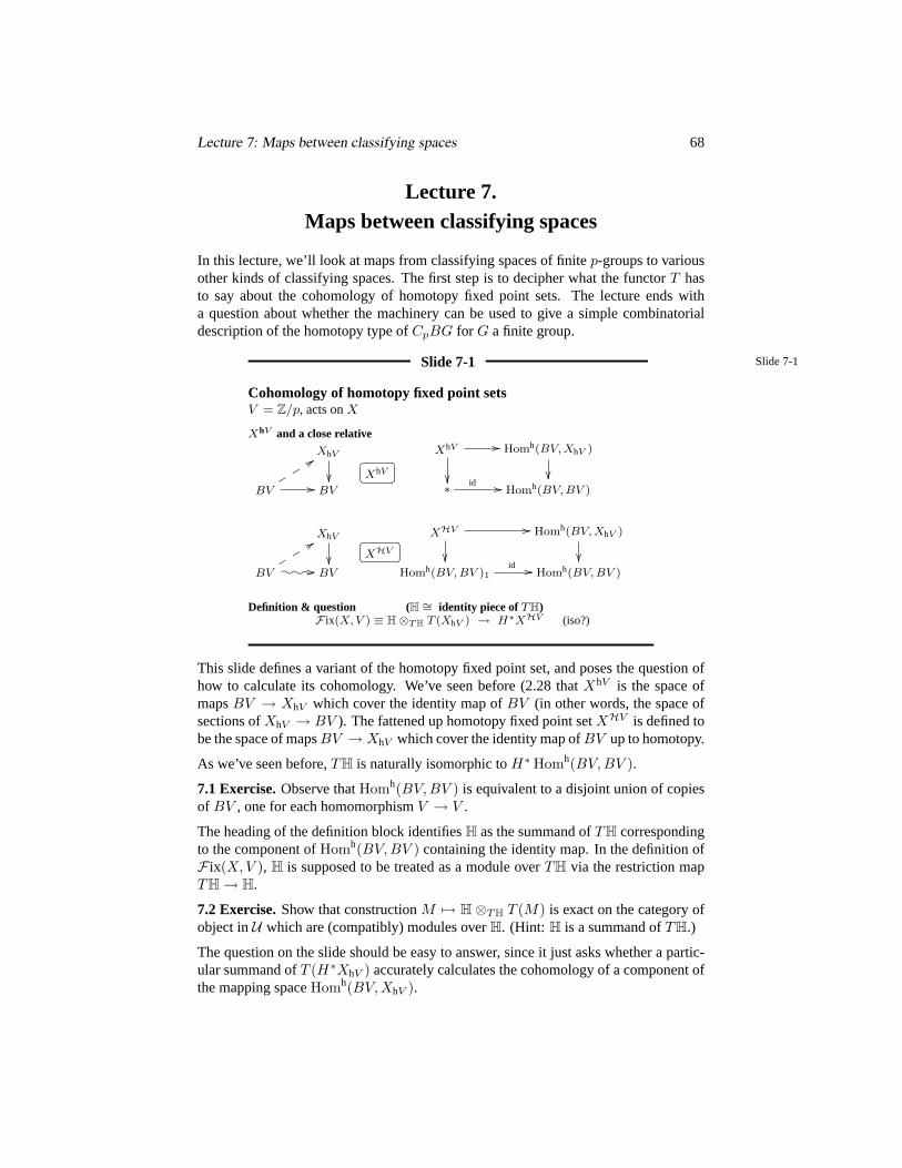
Lecture 7: Maps between classifying spaces 68
Lecture 7.Maps between classifying spaces
In this lecture, we’ll look at maps from classifying spaces of finitep-groups to variousother kinds of classifying spaces. The first step is to decipher what the functorT hasto say about the cohomology of homotopy fixed point sets. The lecture ends witha question about whether the machinery can be used to give a simple combinatorialdescription of the homotopy type ofCpBG for G a finite group.
Slide 7-1 Slide 7-1
Cohomology of homotopy fixed point setsV = Z/p, acts onX
XhV and a close relative
XhV
BV
99rr
r// BV
XhV
XhV //
Homh(BV, XhV )
∗ id // Homh(BV, BV )
XhV
BV
99rr
r///o/o/o BV
XHV
XHV //
Homh(BV, XhV )
Homh(BV, BV )1
id // Homh(BV, BV )
Definition & question (H ∼= identity piece ofTH)F ix(X, V ) ≡ H⊗T H T (XhV ) → H∗XHV (iso?)
This slide defines a variant of the homotopy fixed point set, and poses the question ofhow to calculate its cohomology. We’ve seen before (2.28 thatXhV is the space ofmapsBV → XhV which cover the identity map ofBV (in other words, the space ofsections ofXhV → BV ). The fattened up homotopy fixed point setXHV is defined tobe the space of mapsBV → XhV which cover the identity map ofBV up to homotopy.
As we’ve seen before,TH is naturally isomorphic toH∗ Homh(BV,BV ).
7.1 Exercise.Observe thatHomh(BV,BV ) is equivalent to a disjoint union of copiesof BV , one for each homomorphismV → V .
The heading of the definition block identifiesH as the summand ofTH correspondingto the component ofHomh(BV,BV ) containing the identity map. In the definition ofF ix(X, V ), H is supposed to be treated as a module overTH via the restriction mapTH→ H.
7.2 Exercise.Show that constructionM 7→ H⊗TH T (M) is exact on the category ofobject inU which are (compatibly) modules overH. (Hint: H is a summand ofTH.)
The question on the slide should be easy to answer, since it just asks whether a partic-ular summand ofT (H∗XhV ) accurately calculates the cohomology of a component ofthe mapping spaceHomh(BV,XhV ).
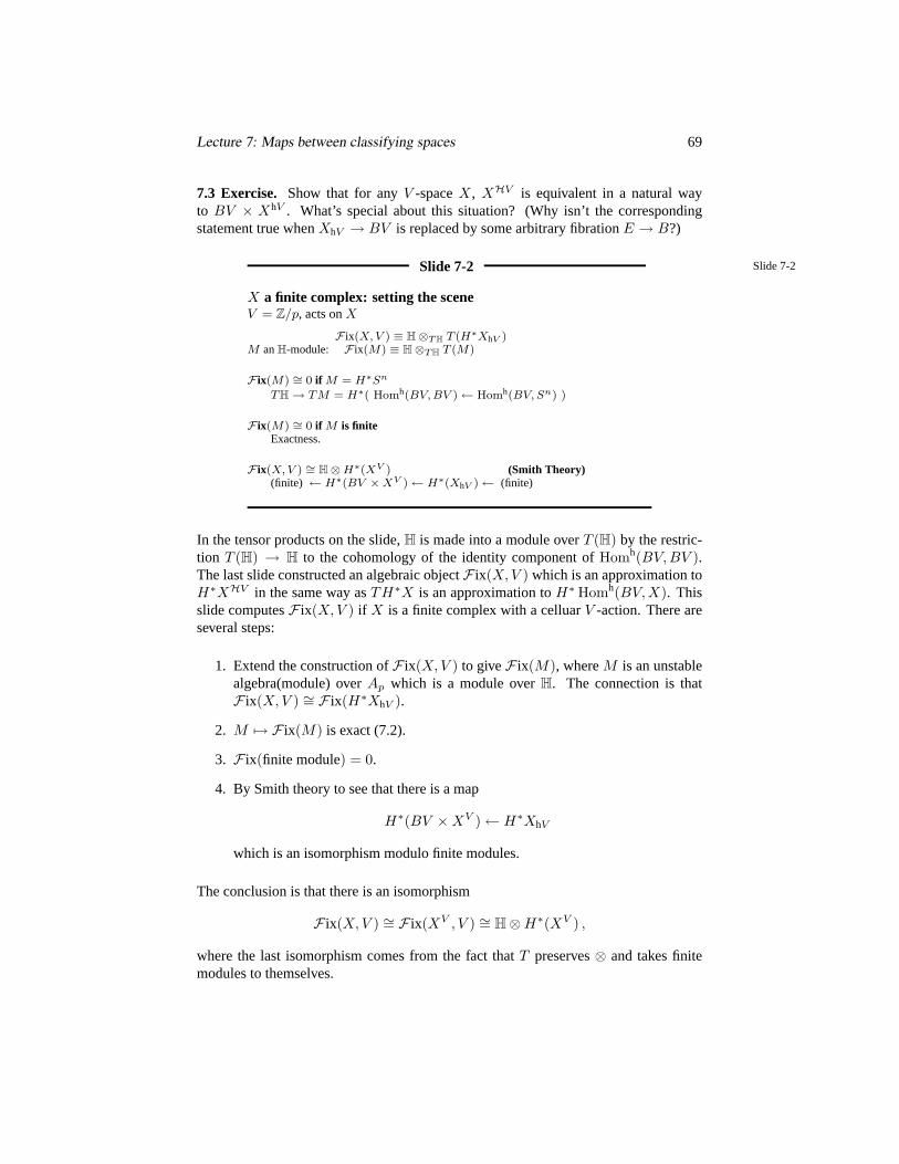
Lecture 7: Maps between classifying spaces 69
7.3 Exercise. Show that for anyV -spaceX, XHV is equivalent in a natural wayto BV × XhV . What’s special about this situation? (Why isn’t the correspondingstatement true whenXhV → BV is replaced by some arbitrary fibrationE → B?)
Slide 7-2 Slide 7-2
X a finite complex: setting the sceneV = Z/p, acts onX
F ix(X, V ) ≡ H⊗T H T (H∗XhV )M anH-module: F ix(M) ≡ H⊗T H T (M)
F ix(M) ∼= 0 if M = H∗Sn
TH→ TM = H∗( Homh(BV, BV )← Homh(BV, Sn) )
F ix(M) ∼= 0 if M is finiteExactness.
F ix(X, V ) ∼= H⊗H∗(XV ) (Smith Theory)(finite) ← H∗(BV ×XV )← H∗(XhV )← (finite)
In the tensor products on the slide,H is made into a module overT (H) by the restric-tion T (H) → H to the cohomology of the identity component ofHomh(BV,BV ).The last slide constructed an algebraic objectF ix(X, V ) which is an approximation toH∗XHV in the same way asTH∗X is an approximation toH∗ Homh(BV,X). Thisslide computesF ix(X, V ) if X is a finite complex with a celluarV -action. There areseveral steps:
1. Extend the construction ofF ix(X, V ) to giveF ix(M), whereM is an unstablealgebra(module) overAp which is a module overH. The connection is thatF ix(X, V ) ∼= F ix(H∗XhV ).
2. M 7→ F ix(M) is exact (7.2).
3. F ix(finite module) = 0.
4. By Smith theory to see that there is a map
H∗(BV ×XV )← H∗XhV
which is an isomorphism modulo finite modules.
The conclusion is that there is an isomorphism
F ix(X, V ) ∼= F ix(XV , V ) ∼= H⊗H∗(XV ) ,
where the last isomorphism comes from the fact thatT preserves⊗ and takes finitemodules to themselves.

Lecture 7: Maps between classifying spaces 70
7.4 Exercise. In computingF ix(H∗Sn), H∗Sn is treated as a trivial module overH, in other words, as a module in which the action factors through the unique ringhomomorphismH→ Fp. Verify thatF ix(H∗Sn) is zero, and show carefully how thisimplies thatF ix(M) = 0 for any finite moduleM . (You may need to use a little bit ofinterplay betweenT on the categoryK of unstable algebras andT on the categoryUof unstable modules).
Slide 7-3 Slide 7-3
X a finite complex (II)V = Z/p, acts onX
BV ×XV is a volunteer for(CpX)HV !
Theorem(CpX)HV ∼ BV × Cp(XV )
(CpX)hV ∼ Cp(XV )
Corollary ( T -free, V -free)Q a finitep-group,X a finiteQ-complex =⇒
(CpX)hQ ∼ Cp(XQ)
7.5 Exercise.There is a little sleight of hand hidden behind the innocent slide. Thefact that(CpX)HV appears depends on the equivalence
Cp(XhV ) ∼ (CpX)hV
Show that this follows from the fibre lemma (slide 5–10).
7.6 Exercise.Prove the corollary on the slide, using induction on the size ofQ.
Slide 7-4 Slide 7-4
Aside: sighting ofCp(p-bad space)
• Y = S1 ∨ S1
• X = Y ∗ S1 ∗ S1 ∗ · · · ∗ S1
• Q = Z/p
• Q-actions: trivial onY , rotation onS1, diagonal onX
Y has problems (CpY 6= LpY , CpCpY 6= CpY . . .)
p-bad news(CpX)hQ ∼p CpY
You can run but you can’t hide.
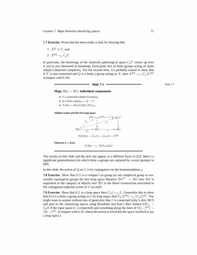
Lecture 7: Maps between classifying spaces 71
7.7 Exercise.Prove that the news really is bad, by showing that
1. XQ ∼= Y , and
2. XhQ ∼p CpY
In particular, the homology of the relatively pathological spaceCpY comes up evenif you’re just interested in homotopy fixed point sets of finite groups acting on finitesimply-connected complexes. For the second item, it’s probably easiest to show thatif X is one-connected andQ is a finitep-group acting onX, thenXhQ ∼p (CpX)hQ
(compare with 6.10).
Slide 7-5 Slide 7-5
Maps BQ→ BG: individual components
• G a connected compact Lie group,
• Q a finitep-group,ρ : Q→ G
• Z(Bρ) = Homh(BQ, BG)Bρ
Adjoint action and the free loop space
EG×G (Gad)∼ //
BGS1
BQ
Bρ//
λ2
99ss
ss
siiiiii
44iiiiii λ1
BG =// BG
ΩZ(Bρ) ∼ λ1’s ∼ λ2’s ∼ GhQ
Theorem (Cp-free)Z(Bρ) ∼p B(ZG(ρQ))
The results on this slide and the next one appear in a different form in [32]; there’s asignificant generalization (in which finitep-groups are replaced byp-toral groups) in[80].
In this slide, the action ofQ onG is by conjugation via the homomorphismρ.
7.8 Exercise.Show that ifG is a compact Lie group (or any simplicial group or rea-sonable topological group) the free loop space fibrationBGS1 → BG over BG isequivalent in the category of objects overBG to the Borel construction associated tothe conjugation (adjoint) action ofG on itself.
7.9 Exercise.Show that ifL is a loop space thenCpL ∼p L. Generalize this to showthat if Q is a finitep-group acting onL by loop maps, thenCp(LhQ) ∼p (CpL)hQ. Youmight want to assume without loss of generality thatL is connected (why is this OK?)and pass to the classifying spaces using Bousfield and Kan’s fibre lemma (ΩCp ∼CpΩ if the input space is1-connected) and something along the lines ofΩ((−)hQ) ∼(Ω(−))hQ. (Compare with 6.10, where the action is trivial but the space involved is nota loop space.)
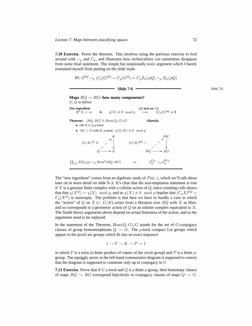
Lecture 7: Maps between classifying spaces 72
7.10 Exercise.Prove the theorem. This involves using the previous exercise to foolaround with∼p andCp, and illustrates how technicalities can sometimes disappearfrom some final statement. The simple but notationally toxic argument which I barelyrestrained myself from putting on the slide reads
Pf: GhQ ∼p (CpG)hQ ∼ Cp(GQ) = CpZG(ρQ) ∼p ZG(ρQ)
Slide 7-6 Slide 7-6
Maps BQ→ BG: how many components?G, Q as before
New ingredient (Q acts onX)H∗X <∞ & χ(X) 6= 0 mod p =⇒ (CpX)hQ 6= ∅
Theorem: [BQ, BG] ∼= Hom(Q, G)/G (Sketch)• OK if G is p-toral
• ∃K ⊂ G with K p-toral, χ(G/K) 6= 0 mod p
(G/K)Q ∼=
K
Q
????
?// G
(G/K)hQ ∼
BK
BQ
<<yy
yy
// BG
‘〈ρ〉 BZG(ρ) ∼p Homh(BQ, BG) ⇔ CCQ
G ∼p ChCQ
G
The “new ingredient” comes from an algebraic study ofF ix(–), which we’ll talk aboutlater on in more detail on slide 9–3. It’s clear that the non-emptiness statement is trueif X is a genuine finite complex with a cellular action ofQ, since counting cells showsthat thatχ(XQ) = χ(X) mod p, and soχ(X) 6= 0 mod p implies that(CpX)hQ ∼Cp(XQ) is nonempty. The problem is that here we have to handle a case in whichthe “action” of Q on X (= G/K) arises from a fibration overBQ with X as fibre,and so corresponds to a geometric action ofQ on an infinite complex equivalent toX.The Smith theory arguments above depend on actual finiteness of the action, and so thearguments need to be replaced.
In the statement of the Theorem,Hom(Q,G)/G stands for the set ofG-conjugacyclasses of group homomorphismsQ → G. The p-toral compact Lie groups whichappear in the proof are groups which fit into an exact sequence
1→ T → K → P → 1
in whichT is a torus (a finite product of copies of the circle group) andP is a finitep-group. The squiggly arrow in the left-hand commutative diagram is supposed to conveythat the diagram is supposed to commute only up to conjugacy inG
7.11 Exercise.Prove that ifG p-toral andQ is a finitep-group, then homotopy classesof mapsBQ → BG correspond bijectively to conjugacy classes of mapsQ → G.

Lecture 7: Maps between classifying spaces 73
One way to do this is by inspecting the extension in whichG by definition sits (thestatement is pretty clear ifG is a torus or a finitep-group). Here’s another approach.Show that it is possible to find a commutative diagram
1 // (Z/p∞)r //
G′ //
P //
1
1 // (S1)r // G // P // 1
in which the left vertical arrow is the inclusion of thep-primary torsion subgroup of(S1)r. (Don’t make the mistake of takingG′ to be the set ofp-primary torsion elementsin G; this isn’t necessarily a subgroup.) Now show that there is a fibration sequence
(BZ[1/p])r // BG′ // BG
and use this to compareHomh(BQ, BG′) to Homh(BQ, BG), as well as to compareHom(Q,G′)/G′ to Hom(Q,G)/G.
The subgroupK of G which appears on the slide is the “p-normalizer” NpT of amaximal torusT in G. This is the inverse image in the normalizerNT of T of aSylowp-subgroup of the Weyl groupW = (NT )/T . Note that the Euler characteristicχ(G/NT ) is 1.
7.12 Exercise.Try to make some sense of the “proof” which is sketched for the the-orem. The argument has something to do with the fact that in light of the previousdiscussion there is a connection (involving occasional insertion and/or deletion ofCp)between(G/K)Q and(G/K)hQ. But the space(G/K)Q only makes sense if thereis a homomorphismQ → G to look at. How does the “new ingredient” contribute toshowing that any mapBQ→ BG is obtained from a homomorphismQ→ G?
The last statement on the slide is an interpretation of the calculation we’ve made on thisslide and the previous one; the interpretation is in the language of homotopy theories.The statement is that ifQ andG are interpreted as categories enriched over topologicalspaces, i.e., homotopy theories, then the category of functors fromQ to G is Z/p-equivalent, as an enriched category, to the derived or homotopy-invariant category offunctors fromQ to G.
7.13 Exercise.(see 1.2) A functorCQ → CG is just a group homomorphismρ : Q →G. A morphism between two such functors is an elementg ∈ G with gρg−1 = ρ′.What does this have to do with
∐〈ρ〉 BZG(ρ)?
The following exercise shows that maps from the classifying space of a finite groupinto the classifying space of a compact connected Lie group are not directly related togroup homomorphisms if more than one prime divides the order of the finite group.
7.14 Exercise.Produce a mapBΣ3 → BS3 which is not realized by any ho-momorphismΣ3 → S3. HereΣ3 is the symmetric group on3 letters (or equiva-
lently the unique nontrivial semidirect productZ/2nZ/3) andS3 is the multiplicativegroup of unit quaternions (or equivalently the special unitary groupSU(2)). It might
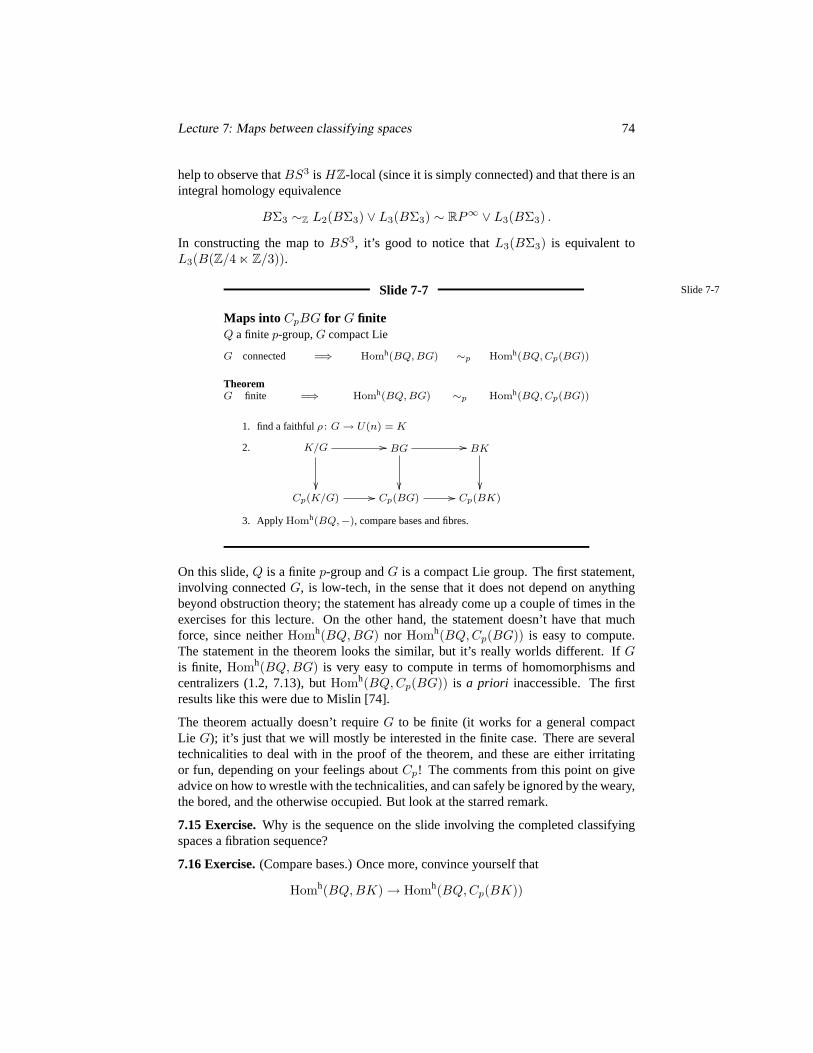
Lecture 7: Maps between classifying spaces 74
help to observe thatBS3 is HZ-local (since it is simply connected) and that there is anintegral homology equivalence
BΣ3 ∼Z L2(BΣ3) ∨ L3(BΣ3) ∼ RP∞ ∨ L3(BΣ3) .
In constructing the map toBS3, it’s good to notice thatL3(BΣ3) is equivalent toL3(B(Z/4 n Z/3)).
Slide 7-7 Slide 7-7
Maps into CpBG for G finiteQ a finitep-group,G compact Lie
G connected =⇒ Homh(BQ, BG) ∼p Homh(BQ, Cp(BG))
TheoremG finite =⇒ Homh(BQ, BG) ∼p Homh(BQ, Cp(BG))
1. find a faithfulρ : G→ U(n) = K
2. K/G //
BG //
BK
Cp(K/G) // Cp(BG) // Cp(BK)
3. Apply Homh(BQ,−), compare bases and fibres.
On this slide,Q is a finitep-group andG is a compact Lie group. The first statement,involving connectedG, is low-tech, in the sense that it does not depend on anythingbeyond obstruction theory; the statement has already come up a couple of times in theexercises for this lecture. On the other hand, the statement doesn’t have that muchforce, since neitherHomh(BQ, BG) nor Homh(BQ, Cp(BG)) is easy to compute.The statement in the theorem looks the similar, but it’s really worlds different. IfGis finite, Homh(BQ, BG) is very easy to compute in terms of homomorphisms andcentralizers (1.2, 7.13), butHomh(BQ, Cp(BG)) is a priori inaccessible. The firstresults like this were due to Mislin [74].
The theorem actually doesn’t requireG to be finite (it works for a general compactLie G); it’s just that we will mostly be interested in the finite case. There are severaltechnicalities to deal with in the proof of the theorem, and these are either irritatingor fun, depending on your feelings aboutCp! The comments from this point on giveadvice on how to wrestle with the technicalities, and can safely be ignored by the weary,the bored, and the otherwise occupied. But look at the starred remark.
7.15 Exercise.Why is the sequence on the slide involving the completed classifyingspaces a fibration sequence?
7.16 Exercise.(Compare bases.) Once more, convince yourself that
Homh(BQ, BK)→ Homh(BQ, Cp(BK))
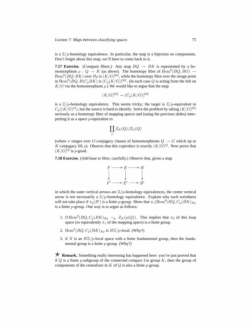
Lecture 7: Maps between classifying spaces 75
is aZ/p-homology equivalence. In particular, the map is a bijection on components.Don’t forget about this map; we’ll have to come back to it.
7.17 Exercise. (Compare fibres.) Any mapBQ → BK is represented by a ho-momorphismρ : Q → K (as above). The homotopy fibre ofHomh(BQ, BG) →Homh(BQ, BK) overBρ is (K/G)hQ, while the homotopy fibre over the image pointin Homh(BQ, B(CpBK) is (Cp(K/G))hQ. (In each caseQ is acting from the left onK/G via the homomorphismρ.) We would like to argue that the map
(K/G)hQ → (Cp(K/G))hQ
is a Z/p-homology equivalence. This seems tricky; the target isZ/p-equivalent toCp((K/G)Q), but the source is hard to identify. Solve the problem by taking(K/G)hQ
seriously as a homotopy fibre of mapping spaces and (using the previous slides) inter-preting it as a spacep-equivalent to∐
σ
ZK(Q)/ZG(Q)
(whereσ ranges overG-conjugacy classes of homomorphismsQ → G which up toK-conjugacy liftρ). Observe that this coproduct is exactly(K/G)Q. Now prove that(K/G)Q is p-good.
7.18 Exercise.(Add base to fibre, carefully.) Observe that, given a map
F //
E //
B
F ′ // E′ // B′
in which the outer vertical arrows areZ/p-homology equivalences, the center verticalarrow isnot necessarily aZ/p-homology equivalence. Explain why such weirdnesswill not take place ifπq(B′) is a finitep-group. Show thatπ1(Homh(BQ, Cp(BK)Bρ
is a finitep-group. One way is to argue as follows:
1. Ω Homh(BQ, Cp(BK)Bρ ∼p ZK(ρ(Q)). This implies thatπ0 of this loopspace (or equivalentlyπ1 of the mapping space) is a finite group.
2. Homh(BQ, Cp(BK)Bρ is HZ/p-local. (Why?)
3. if X is anHZ/p-local space with a finite fundamental group, then the funda-mental group is a finitep-group. (Why?)
? Remark. Something really interesting has happened here: you’ve just proved thatif Q is a finitep-subgroup of the connected compact Lie groupK, then the group ofcomponents of the centralizer inK of Q is also a finitep-group.
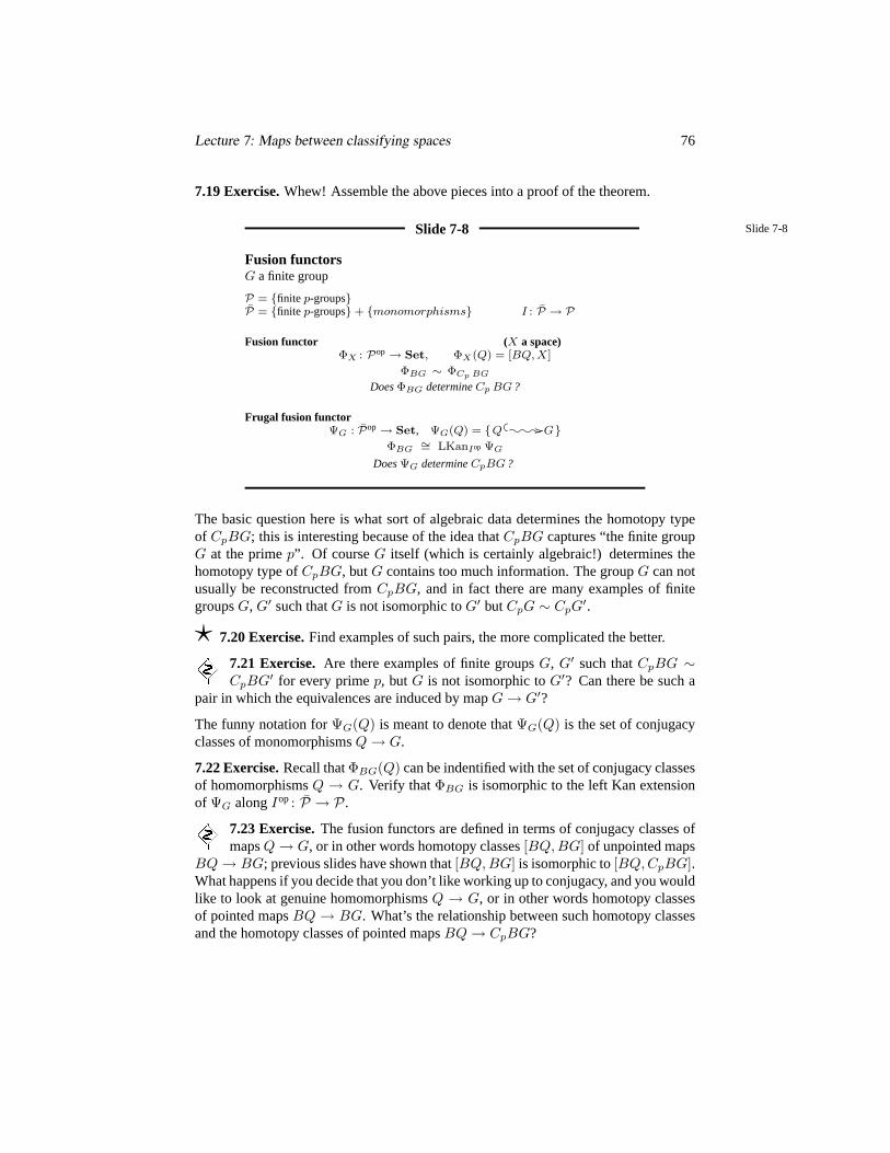
Lecture 7: Maps between classifying spaces 76
7.19 Exercise.Whew! Assemble the above pieces into a proof of the theorem.
Slide 7-8 Slide 7-8
Fusion functorsG a finite group
P = finite p-groupsP = finite p-groups + monomorphisms I : P → P
Fusion functor (X a space)ΦX : Pop→ Set, ΦX(Q) = [BQ, X]
ΦBG ∼ ΦCp BG
DoesΦBG determineCp BG ?
Frugal fusion functorΨG : Pop→ Set, ΨG(Q) = Q ///o/o/o G
ΦBG∼= LKanIop ΨG
DoesΨG determineCpBG ?
The basic question here is what sort of algebraic data determines the homotopy typeof CpBG; this is interesting because of the idea thatCpBG captures “the finite groupG at the primep”. Of courseG itself (which is certainly algebraic!) determines thehomotopy type ofCpBG, butG contains too much information. The groupG can notusually be reconstructed fromCpBG, and in fact there are many examples of finitegroupsG, G′ such thatG is not isomorphic toG′ butCpG ∼ CpG
′.
? 7.20 Exercise.Find examples of such pairs, the more complicated the better.
7.21 Exercise.Are there examples of finite groupsG, G′ such thatCpBG ∼CpBG′ for every primep, but G is not isomorphic toG′? Can there be such a
pair in which the equivalences are induced by mapG→ G′?
The funny notation forΨG(Q) is meant to denote thatΨG(Q) is the set of conjugacyclasses of monomorphismsQ→ G.
7.22 Exercise.Recall thatΦBG(Q) can be indentified with the set of conjugacy classesof homomorphismsQ → G. Verify thatΦBG is isomorphic to the left Kan extensionof ΨG alongIop: P → P.
7.23 Exercise.The fusion functors are defined in terms of conjugacy classes ofmapsQ→ G, or in other words homotopy classes[BQ, BG] of unpointed maps
BQ→ BG; previous slides have shown that[BQ, BG] is isomorphic to[BQ, CpBG].What happens if you decide that you don’t like working up to conjugacy, and you wouldlike to look at genuine homomorphismsQ → G, or in other words homotopy classesof pointed mapsBQ → BG. What’s the relationship between such homotopy classesand the homotopy classes of pointed mapsBQ→ CpBG?
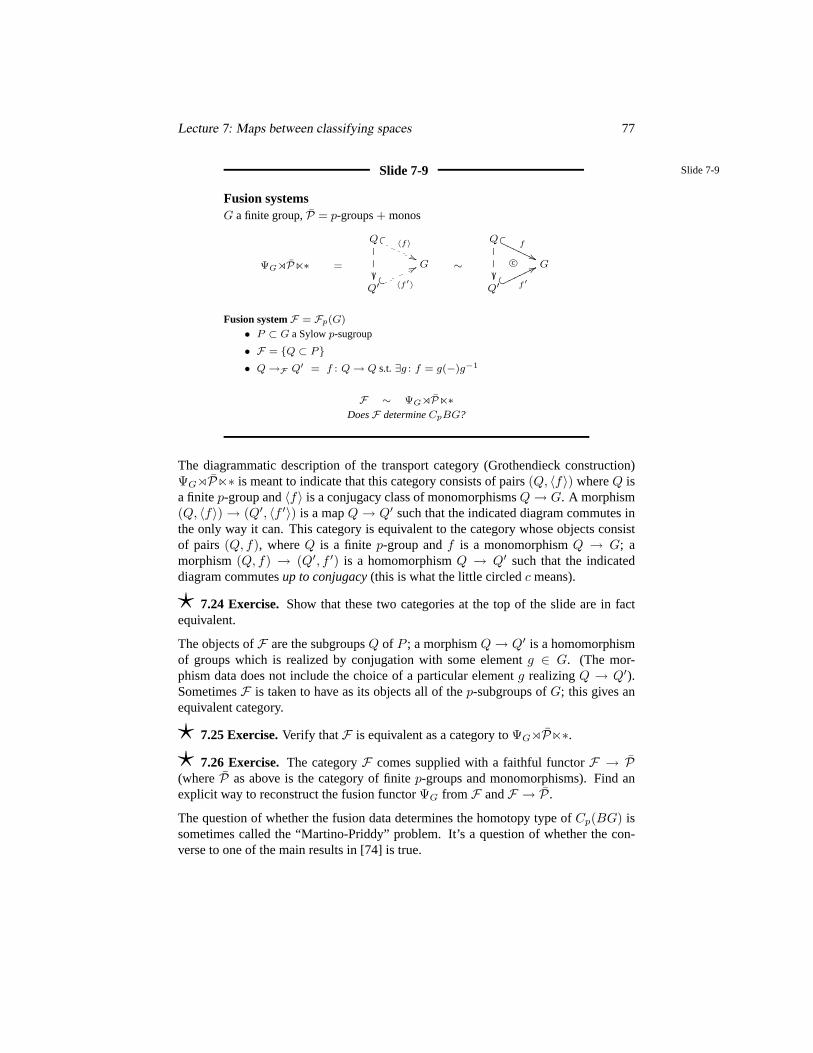
Lecture 7: Maps between classifying spaces 77
Slide 7-9 Slide 7-9
Fusion systemsG a finite group,P = p-groups+ monos
ΨGoPn∗ =
Q
u〈f〉
''G
Q′* 〈f ′〉
77 ∼
Q
c©
uf
''PPPPPP
G
Q′*
f ′
77oooooo
Fusion systemF = Fp(G)
• P ⊂ G a Sylowp-sugroup
• F = Q ⊂ P• Q→F Q′ = f : Q→ Q s.t.∃g : f = g(−)g−1
F ∼ ΨGoPn∗DoesF determineCpBG?
The diagrammatic description of the transport category (Grothendieck construction)ΨGoPn∗ is meant to indicate that this category consists of pairs(Q, 〈f〉) whereQ isa finitep-group and〈f〉 is a conjugacy class of monomorphismsQ→ G. A morphism(Q, 〈f〉)→ (Q′, 〈f ′〉) is a mapQ→ Q′ such that the indicated diagram commutes inthe only way it can. This category is equivalent to the category whose objects consistof pairs (Q, f), whereQ is a finitep-group andf is a monomorphismQ → G; amorphism(Q, f) → (Q′, f ′) is a homomorphismQ → Q′ such that the indicateddiagram commutesup to conjugacy(this is what the little circledc means).
? 7.24 Exercise.Show that these two categories at the top of the slide are in factequivalent.
The objects ofF are the subgroupsQ of P ; a morphismQ→ Q′ is a homomorphismof groups which is realized by conjugation with some elementg ∈ G. (The mor-phism data does not include the choice of a particular elementg realizingQ → Q′).SometimesF is taken to have as its objects all of thep-subgroups ofG; this gives anequivalent category.
? 7.25 Exercise.Verify thatF is equivalent as a category toΨGoPn∗.
? 7.26 Exercise.The categoryF comes supplied with a faithful functorF → P(whereP as above is the category of finitep-groups and monomorphisms). Find anexplicit way to reconstruct the fusion functorΨG fromF andF → P.
The question of whether the fusion data determines the homotopy type ofCp(BG) issometimes called the “Martino-Priddy” problem. It’s a question of whether the con-verse to one of the main results in [74] is true.

Lecture 8: Linking systems and p-local classifying spaces 78
Lecture 8.
Linking systems andp-local classifying spaces
Slide 8-1 Slide 8-1
DoesF determineCpBG?G a finite group,F = Fp(G)
F ∼ Q 〈f〉 //G
Centralizer diagram=⇒ something missing (C = Q ⊂ G)CpBG ∼p hocolimF J J : 〈f〉 7→ BZG(fQ)
Troubling questions1. NeedF and J (better,CpJ) to getCpBG?
2. J too fancy? CpBZG(fQ) not “algebraic”
3. Circular scam? J(1→ G) = BG ∼p CpBG
Solution to (2) and (3):find better C
Let C be the collection of allp-subgroups ofBG (4–3). The categoryF is equivalentto the category which parametrizes the centralizer decomposition forBG which isassociated to the collectionC. We continue to look at the question of whetherFdetermines the homotopy type ofCpBG.
8.1 Exercise.Verify that the collectionC of all nontrivial p-subgroups ofG satisfiesthe condition from 4–5, i.e.
(KC)hG ∼p BG .
(In fact, show thatKC is contractible.) This implies that the homotopy colimit of thecentralizer diagram associated toC is Z/p-equivalent toBG.
The slide points out that we should not expectF itself to giveCpBG, since (accordingto the lore of the centralizer decomposition) theZ/p-homology type ofBG is given bythe homotopy colimit of a highly nontrivial functorJ onF . So what should we do?Accepting the functorJ or evenCpJ as part of the structure is not an attractive option,since the values ofCpJ are complicated, and in fact one of these values is the veryobject,CpBG, which we would like to understand. Remember, the goal here is to finda some sort of data which
1. is reasonably simple and combinatorial,
2. determines the homotopy type ofCpBG, and
3. can be derived from the homotopy type ofCpBG.
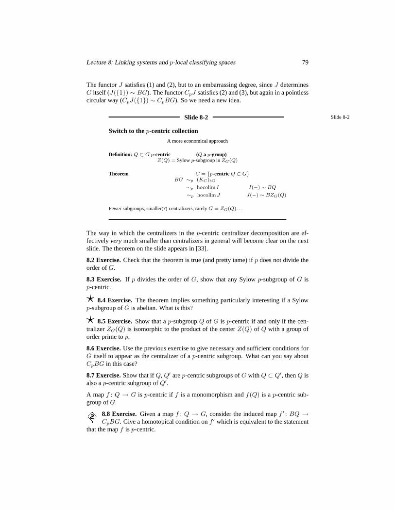
Lecture 8: Linking systems and p-local classifying spaces 79
The functorJ satisfies (1) and (2), but to an embarrassing degree, sinceJ determinesG itself (J(1) ∼ BG). The functorCpJ satisfies (2) and (3), but again in a pointlesscircular way (CpJ(1) ∼ CpBG). So we need a new idea.
Slide 8-2 Slide 8-2
Switch to thep-centric collection
A more economical approach
Definition: Q ⊂ G p-centric (Q a p-group)Z(Q) = Sylowp-subgroup inZG(Q)
Theorem C = p-centric Q ⊂ GBG ∼p (KC)hG
∼p hocolim I I(−) ∼ BQ
∼p hocolim J J(−) ∼ BZG(Q)
Fewer subgroups, smaller(?) centralizers, rarelyG = ZG(Q). . .
The way in which the centralizers in thep-centric centralizer decomposition are ef-fectively verymuch smaller than centralizers in general will become clear on the nextslide. The theorem on the slide appears in [33].
8.2 Exercise.Check that the theorem is true (and pretty tame) ifp does not divide theorder ofG.
8.3 Exercise. If p divides the order ofG, show that any Sylowp-subgroup ofG isp-centric.
? 8.4 Exercise.The theorem implies something particularly interesting if a Sylowp-subgroup ofG is abelian. What is this?
? 8.5 Exercise.Show that ap-subgroupQ of G is p-centric if and only if the cen-tralizerZG(Q) is isomorphic to the product of the centerZ(Q) of Q with a group oforder prime top.
8.6 Exercise.Use the previous exercise to give necessary and sufficient conditions forG itself to appear as the centralizer of ap-centric subgroup. What can you say aboutCpBG in this case?
8.7 Exercise.Show that ifQ, Q′ arep-centric subgroups ofG with Q ⊂ Q′, thenQ isalso ap-centric subgroup ofQ′.
A mapf : Q → G is p-centric if f is a monomorphism andf(Q) is ap-centric sub-group ofG.
8.8 Exercise.Given a mapf : Q → G, consider the induced mapf ′ : BQ →CpBG. Give a homotopical condition onf ′ which is equivalent to the statement
that the mapf is p-centric.
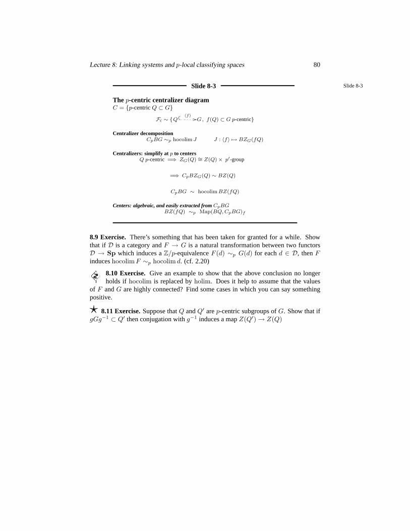
Lecture 8: Linking systems and p-local classifying spaces 80
Slide 8-3 Slide 8-3
The p-centric centralizer diagramC = p-centricQ ⊂ G
Fc ∼ Q 〈f〉 //G, f(Q) ⊂ G p-centric
Centralizer decompositionCpBG ∼p hocolim J J : 〈f〉 7→ BZG(fQ)
Centralizers: simplify at p to centersQ p-centric =⇒ ZG(Q) ∼= Z(Q)× p′-group
=⇒ CpBZG(Q) ∼ BZ(Q)
CpBG ∼ hocolim BZ(fQ)
Centers: algebraic, and easily extracted fromCpBGBZ(fQ) ∼p Map(BQ, CpBG)f
8.9 Exercise. There’s something that has been taken for granted for a while. Showthat if D is a category andF → G is a natural transformation between two functorsD → Sp which induces aZ/p-equivalenceF (d) ∼p G(d) for eachd ∈ D, thenFinduceshocolim F ∼p hocolim d. (cf. 2.20)
8.10 Exercise. Give an example to show that the above conclusion no longerholds if hocolim is replaced byholim. Does it help to assume that the values
of F andG are highly connected? Find some cases in which you can say somethingpositive.
? 8.11 Exercise.Suppose thatQ andQ′ arep-centric subgroups ofG. Show that ifgGg−1 ⊂ Q′ then conjugation withg−1 induces a mapZ(Q′)→ Z(Q)

Lecture 8: Linking systems and p-local classifying spaces 81
Slide 8-4 Slide 8-4
The categoricalp-centric centralizer modelFc = 〈f〉 : f : Q → G p-centric
FunctorZ : Fc→ Grpd, Z(〈f〉) ∼ Z(Q)
Grothendieck constructionCpBG ∼p hocolim BZ
∼p N(Z o Fc)
F vs.Z o Fc
F ∼
Q
// G
gZG(Q)
Q′ // G
Z o Fc ∼
Q
p.-c // G
gZ′G(Q)
Q′ p.-c // G
ZG(Q) ∼= Z(Q)× Z′G(Q)
The slide claims thatZoFc is equivalent to the category whose objects consist of pairs(Q, f), wheref is a monomorphismQ→ G with p-centric image. A homomorphism(Q, f) → (Q′, f ′) is a homomorphismQ → Q′ together with a cosetgZ ′
G(Q) suchthat the mapQ→ Q′ is realized inside ofG by g(−)g−1.
8.12 Exercise.Verify that these morphisms really can be composed.
8.13 Exercise.DescribeZ oFc up to equivalence as a category whose objects are thesubgroups of a given Sylowp-subgroup ofG,
Probably the easiest way to represent the functorZ is by the following formula
Z(〈f〉) = Π(p)1 Homh(BQ, BG)〈f〉 .
The right-had side denotes thep-primary part of the fundamental groupoid of the com-ponent of the space of mapsBQ → BG corresponding to the conjugacy class〈f〉of homomorphismsQ → G. This is also thep-primary part of the component of thecategory of functorsCQ → CG corresponding tof .
8.14 Exercise.Suppose thatH is a connected groupoid with the property that eachvertex group is the product of a finite abelianp-group and a finite group of order primeto p. Convince yourself that the “p-primary part” of this groupoid makes functorialsense (as a groupoid with the same objects aH). If in doubt, think aboutΠ1Cp N(H).
? 8.15 Exercise.Check that the assertions on the slide are correct.
1. The functorZ makes sense,
2. there is a natural transformation from the centralizer decomposition functorJfor thep-centric collection (slide 8–1) into the functorBZ which gives aZ/p-homology equivalenceJ → BZ, and
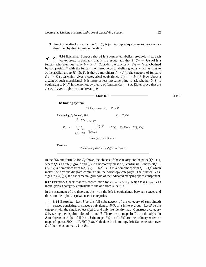
Lecture 8: Linking systems and p-local classifying spaces 82
3. the Grothendieck constructionZoFc is (at least up to equivalence) the categorydescribed by the picture on the slide.
8.16 Exercise.Suppose thatA is a connected abelian groupoid (i.e., eachvertex group is abelian), thatG is a group, and thatI : CG → Grpd is a
functor whose unique valueI(∗) isA. Consider the functorJ : CG → Grp obtainedby composingF with the functor from groupoids to abelian groups which assigns toA the abelian groupH1 N(A). Is there a morphismJ → I (in the category of functorsCG → Grpd) which gives a categorical equivalenceJ(∗) → I(∗)? How about azigzag of such morphisms? It is more or less the same thing to ask whetherN(I) isequivalent toN(J) in the homotopy theory of functorsCG → Sp. Either prove that theanswer is yes or give a counterexample.
Slide 8-5 Slide 8-5
The linking system
Linking systemLc :=Z o Fc
RecoveringLc from CpBG X = CpBG
Fc ∼
Q, BQ
h
Bh
〈f〉:p.c.
**X
Q′, BQ′〈f ′〉:p.c.
44 Z〈f〉 = Π1 Homh(BQ, X)f
Now just formZ o Fc
TheoremCpBG ∼ CpBG′ ⇐⇒ Lc(G) ∼ Lc(G′)
In the diagram formula forFc above, the objects of the category are the pairs(Q, 〈f〉),whereQ is a finitep-group and〈f〉 is a homotopy class ofp-centric (8.8) mapsBQ→CpBG; a homomorphism(Q, 〈f〉) → (Q′, 〈f ′〉) is a homomorphismQ → Q′ whichmakes the obvious diagram commute (in the homotopy category). The functorZ as-signs to(Q, 〈f〉) the fundamental groupoid of the indicated mapping space component.
8.17 Exercise.Check that this construction forLc = Z o Fc, which takesCpBG asinput, gives a category equivalent to the one from slide 8–4.
In the statement of the theorem, the∼ on the left is equivalence between spaces andthe∼ on the right is equivalence of categories.
8.18 Exercise. Let A be the full subcategory of the category of (unpointed)spaces consisting of spaces equivalent toBQ, Q a finitep-group. LetB be the
category with the single objectCpBG and only the identity map. Construct a categoryC by taking the disjoint union ofA andB. There are no maps inC from the object inB to objects inA, but if BQ ∈ A the mapsBQ → CpBG are the ordinaryp-centricmaps of spacesBQ → CpBG (8.8). Calculate the homotopy left Kan extension overC of the inclusion mapA → Sp.

Lecture 8: Linking systems and p-local classifying spaces 83
Slide 8-6 Slide 8-6
Lc vs.Fc – the orbit pictureZG(Q) ∼= Z(Q)× Z′G(Q)
Three categories X = BG, CpBGCategory Object Morphism
Lc Q + fp.c. : BQ→ X h : Q→ Q′∗ + ω
Fc Q + 〈fp.c.〉 ∈ [BQ, X] h : Q→ Q′
Oc Q + 〈fp.c.〉 ∈ [BQ, X] 〈h〉 ∈ [BQ, BQ′]
Three categories
Q
OOO
f :p.c. // G
Q′f ′:p.c.
// G
Lc : gZ′G(Q)
Fc : gZG(Q)
Oc : Q′gZG(Q)
Lc
// Q
Fc
α // Q
Oc
−nQ
>>
β // HoBQ
Conclusions
Q =
BQ
Oc
λ 77oo
oβ
// HoBQ
Fc + α = Oc + β
Lc = Fc + u + λ
This is quite a complicated slide. It gives descriptions for each of three categories;two of these categories we have already run into. The first description is geometric,the second is algebraic; the two descriptions give equivalent categories, not necessarilyisomorphic ones. In part, this systematizes what has appeared before. The symbolXstands for eitherBG or CpBG.
The (p-centric) linking category Lc. From the geometric point of view, an object ofLc is a pair(Q, f), whereQ is a finitep-group andf is ap-centric mapBQ → X. Amap(Q, f)→ (Q′, f ′) is a homomorphismh : Q→ Q′ together with an equivalenceclass of pathsω in Homh(BQ, X) connectingf ′ ·Bh to f . If X = CpBG ths is simplya homotopy class of paths.
8.19 Exercise.How can you describe the equivalence relation on the class of paths ifX = BG? (Remember thatπ1 Homh(BQ, BG)f ∼ BZG(fQ).)
From the algebraic point of view, an object inLc is a pair(Q, f), whereQ is a finitep-group andf : Q → G is a homomorphism. A map(Q, f) → (Q′, f ′) is a homo-morphismh : Q → Q′ together with a cosetgZ ′
G(fQ) of Z ′G(fQ) in G such that
gfg−1 = f ′h.
8.20 Exercise.Convince yourself that these two descriptions give the same category.
The (p-centric) fusion systemFc. From the geometric point of view, an object ofFc
consists of a pair(Q, 〈f〉), whereQ is a finitep-group and〈f〉 is a homotopy classof p-centric mapsBQ → X. A map (Q, 〈f〉) → (Q′, 〈f ′〉) is a homomorphism
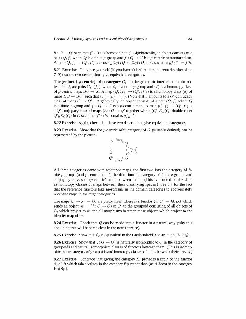
Lecture 8: Linking systems and p-local classifying spaces 84
h : Q→ Q′ such thatf ′ ·Bh is homotopic tof . Algebraically, an object consists of apair (Q, f) whereQ is a finitep-group andf : Q → G is ap-centric homomorphism.A map(Q, f)→ (Q′, f ′) is a cosetgZG(fQ) of ZG(fQ) in G such thatgfg−1 = f ′h.
8.21 Exercise.Convince yourself (if you haven’t before, see the remarks after slide7–9) that the two descriptions give equivalent categories.
The (reduced,p-centric) orbit category Oc. In the geometric interpretation, the ob-jects inOc are pairs(Q, 〈f〉), whereQ is a finitep-group and〈f〉 is a homotopy classof p-centric mapsBQ→ X. A map(Q, 〈f〉)→ (Q′, 〈f ′〉) is a homotopy class〈h〉 ofmapsBQ→ BQ′ such that〈f ′〉 · 〈h〉 = 〈f〉. (Note thath amounts to aQ′-conjugacyclass of mapsQ → Q′.) Algebraically, an object consists of a pair(Q, f) whereQis a finitep-group andf : Q → G is ap-centric map. A map(Q, f) → (Q′, f ′) isa Q′-conjugacy class of maps〈h〉 : Q → Q′ together with a(Q′, ZG(Q) double cosetQ′gZG(Q) in G such thatf ′ · 〈h〉 containsgfg−1.
8.22 Exercise.Again, check that these two descriptions give equivalent categories.
8.23 Exercise.Show that thep-centric orbit category ofG (suitably defined) can berepresented by the picture
Q
OOO
f :p.c. // G Q′g
Q′f ′:p.c.
// G
All three categories come with reference maps, the first two into the category of fi-nite p-groups (andp-centric maps), the third into the category of finitep-groups andconjugacy classes of (p-centric) maps between them. (This is denoted on the slideas homotopy classes of maps between their classifying spaces.) See 8.7 for the factthat the reference functors take morphisms in the domain categories to appropriatelyp-centric maps in the target categories.
The mapsLc → Fc → Oc are pretty clear. There is a functorQ : Oc → Grpd whichsends an objectm = (f : Q → G) of Oc to the groupoid consisting of all objects ofLc which project tom and all morphisms between these objects which project to theidentity map ofm.
8.24 Exercise.Check thatQ can be made into a functor in a natural way (why thisshould be true will become clear in the next exercise).
8.25 Exercise.Show thatLc is equivalent to the Grothendieck constructionOc nQ.
8.26 Exercise.Show thatQ(Q → G) is naturally isomorphic toQ in the category ofgroupoids and natural isomorphism classes of functors between them. (This is isomor-phic to the category of groupoids and homotopy classes of maps between their nerves.)
8.27 Exercise.Conclude that giving the categoryLc provides a liftλ of the functorβ, a lift which takes values in the categorySp rather than (asβ does) in the categoryHo(Sp).
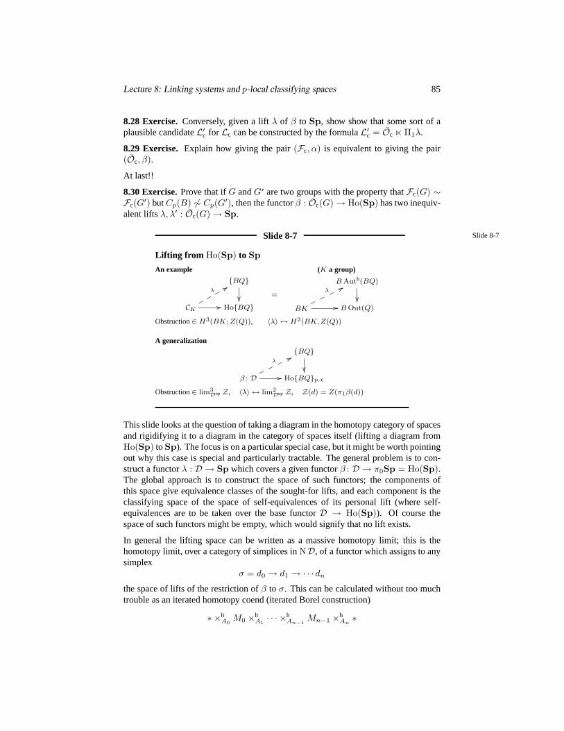
Lecture 8: Linking systems and p-local classifying spaces 85
8.28 Exercise.Conversely, given a liftλ of β to Sp, show show that some sort of aplausible candidateL′c for Lc can be constructed by the formulaL′c = Oc n Π1λ.
8.29 Exercise. Explain how giving the pair(Fc, α) is equivalent to giving the pair(Oc, β).
At last!!
8.30 Exercise.Prove that ifG andG’ are two groups with the property thatFc(G) ∼Fc(G′) butCp(B) 6∼ Cp(G′), then the functorβ : Oc(G)→ Ho(Sp) has two inequiv-alent liftsλ, λ′ : Oc(G)→ Sp.
Slide 8-7 Slide 8-7
Lifting from Ho(Sp) to Sp
An example (K a group)
BQ
CK //
λ88qqqq
HoBQ
=
B Auth(BQ)
BK //
λ77ooooB Out(Q)
Obstruction∈ H3(BK; Z(Q)), 〈λ〉 ↔ H2(BK, Z(Q))
A generalization
BQ
β : D //
λ77nnnn
HoBQp.-c
Obstruction∈ lim3Dop Z, 〈λ〉 ↔ lim2
Dop Z, Z(d) = Z(π1β(d))
This slide looks at the question of taking a diagram in the homotopy category of spacesand rigidifying it to a diagram in the category of spaces itself (lifting a diagram fromHo(Sp) toSp). The focus is on a particular special case, but it might be worth pointingout why this case is special and particularly tractable. The general problem is to con-struct a functorλ : D → Sp which covers a given functorβ : D → π0Sp = Ho(Sp).The global approach is to construct the space of such functors; the components ofthis space give equivalence classes of the sought-for lifts, and each component is theclassifying space of the space of self-equivalences of its personal lift (where self-equivalences are to be taken over the base functorD → Ho(Sp)). Of course thespace of such functors might be empty, which would signify that no lift exists.
In general the lifting space can be written as a massive homotopy limit; this is thehomotopy limit, over a category of simplices inND, of a functor which assigns to anysimplex
σ = d0 → d1 → · · · dn
the space of lifts of the restriction ofβ to σ. This can be calculated without too muchtrouble as an iterated homotopy coend (iterated Borel construction)
∗ ×hA0
M0 ×hA1· · · ×h
An−1Mn−1 ×h
An∗

Lecture 8: Linking systems and p-local classifying spaces 86
whereXi = β(di), Ai = Auth1(Xi) is the identity component of the space of self-
equivalences ofXi, andMi = Homh(Xi, Xi+1)fi is the component of the space ofmapsXi → Xi+1 corresponding tofi = β(di → di+1).
Now for the punch line.
? 8.31 Exercise.Show that if eachXi above is the classifying space of a finitep-groupQi, and each mapfi is ap-centric map, then the above iterated homotopy coendcollapses into
B2ZQn) = K(Z(Qn), 2)
It follows from this and a cofinality argument that the desired space of lifts can be writ-ten as the homotopy limit overD itself of a functor onDop which assigns tod a spaceequivalent toB2Z(d), whereZ(d) = Z(π1β(d)). According to general principles,there is an obstruction inlim3Z which is zero if and only if the space of lifts is nonempty; if this obstruction vanishes, the set of components corresponds bijectively tolim2Z.
8.32 Exercise. Work out these general principles. Here’s one statement.Suppose thatD is a category,A is a functor fromD to abelian groups, and
n ≥ 1 is an integer. Give a classification up to equivalence all functorsF : D →Sp such thatπiF ∼= ∗, i 6= n, andπnF ∼= A; the functors should be in bijectivecorrespondence with elements oflimn+1 A. The classification should be along thelines of the theory ofk-invariants. For instance, the functor has a section, in the sensethatholim F is nonempty, if and only if it corresponds to the zero element oflimn+1 A.If the functordoeshave a section, then the components of the space of sections (i.e., theholim) correspond bijectively tolimn A. (Note thatF is not assumed to be a functorinto pointed spaces, so applyingπnF is probably best interpreted asHn(F ; Z).) If Dis the category of a groupG, what have you recovered?
This explains the bottom half of the slide. The top half describes a simpler problemwhich is meant to put above machinery in a more familiar context. If the categoryDis the category of the groupK, the problem is one of taking an action ofK on BQup to homotopy and rigidifying it to an ordinary action, i.e., lifting a mapBK →P1B Auth(BQ) to a mapBK → B Auth(BQ) or, equivalently, turning an abstractkernel into a group extension. The neatest way to solve this is to analyze the homotopygroups ofB Auth(BQ) and use obstruction theory.
? 8.33 Exercise. Review the obstruction theory. It has already come up, at leastimplicitly, that the only nonvanishing homotopy groups ofB Auth(BQ) (for Q anydiscrete group) are
πi =
Out(Q) i = 1Z(Q) i = 2
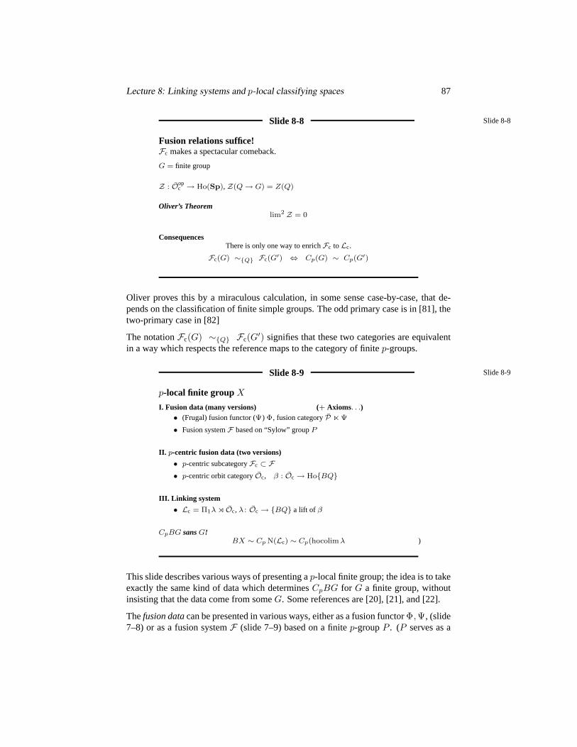
Lecture 8: Linking systems and p-local classifying spaces 87
Slide 8-8 Slide 8-8
Fusion relations suffice!Fc makes a spectacular comeback.
G = finite group
Z : Oopc → Ho(Sp),Z(Q→ G) = Z(Q)
Oliver’s Theoremlim2 Z = 0
ConsequencesThere is only one way to enrichFc toLc.
Fc(G) ∼Q Fc(G′) ⇔ Cp(G) ∼ Cp(G′)
Oliver proves this by a miraculous calculation, in some sense case-by-case, that de-pends on the classification of finite simple groups. The odd primary case is in [81], thetwo-primary case in [82]
The notationFc(G) ∼Q Fc(G′) signifies that these two categories are equivalentin a way which respects the reference maps to the category of finitep-groups.
Slide 8-9 Slide 8-9
p-local finite group X
I. Fusion data (many versions) (+ Axioms. . .)• (Frugal) fusion functor (Ψ) Φ, fusion categoryP n Ψ
• Fusion systemF based on “Sylow” groupP
II. p-centric fusion data (two versions)
• p-centric subcategoryFc ⊂ F• p-centric orbit categoryOc, β : Oc→ HoBQ
III. Linking system
• Lc = Π1λ o Oc, λ : Oc→ BQ a lift of β
CpBG sansG!BX ∼ Cp N(Lc) ∼ Cp(hocolim λ )
This slide describes various ways of presenting ap-local finite group; the idea is to takeexactly the same kind of data which determinesCpBG for G a finite group, withoutinsisting that the data come from someG. Some references are [20], [21], and [22].
Thefusion datacan be presented in various ways, either as a fusion functorΦ,Ψ, (slide7–8) or as a fusion systemF (slide 7–9) based on a finitep-groupP . (P serves as a
Lecture 8: Linking systems and p-local classifying spaces 88
Sylow “p-subgroup” for thep-local finite groups. There are various axioms that implyin particular that it is possible to go back and forth among these presentations.
Thep-centric fusion datasits inside the fusion data. For instance, ifF is described as acategory whose objects are the subgroups ofP and whose morphisms are certain mapsbetween them, thenFc is the subcategory consisting of subgroupsQ such that everyobject inF isomorphic toQ is ap-centric subgroup ofP .
The linking systemis specified in the same way as when a groupG is present. Oneway to do this (not mentioned on the slide) is to describeLc directly as a suitableextension ofFc. Another way is to construct the “orbit category”Oc as a quotientof Fc, notice that the axioms give a functorβ from Oc to the homotopy category ofspaces (actually the homotopy category of classifying spaces of finitep-groups andp-centric maps between these classifying spaces) and then describeLc in terms of a liftλ : Oc → Sp of β. (Of course,λ might not exist if a certain characteristic element inlim3
OcZ refuses to vanish!)

Lecture 9: p-compact groups 89
Lecture 9.
p-compact groups
A p-compact group is meant to be homotopical a analogues of a compact Lie group. Inthis lecture I’ll definep-compact groups and describe how to prove at least some thingsabout them. This is just an introduction to the theory, which has recently produced acomplete classification of the objects [4] [77] [78] [3]. For basic information aboutp-compact groups see [42], [65], or [76].
Slide 9-1 Slide 9-1
Definition of a p-compact groupNot quite likep-local finite groups
DictionaryCompact Lie group p-compact group
groupG loop spaceX
compact, smooth H∗X <∞, BX ∼ CpBX
ρ : G→ H Bρ : BX → BY
ker ρ = 1 H∗fibre(BX → BY ) <∞
H/G Y/X =fibreBX → BY
ZH(ρG) ZY (ρX) = ΩHomh(BX, BY )Bρ
abelian ZX(X) ∼ X
torusT = (S1)r p-complete torusT = CpT
. . . . . .
For p-local finite groups, part of the problem is coming up with the definition; youanalyze thep-completionCpBG for G a finite group and abstract what seem to be itsessential features. The upshot is thatp-local finite groups come with an explicit wayof building them up out of finitep-groups. The case ofp-compact groups is different.The definition is simple:X is ap-compact group ifX is a loop space,H∗X is finite(written on the slide asH∗X < ∞), andBX is p-complete. This is a straightforwardstab at capturing something that looks like a finite loop space(H∗X <∞) but whosehomotopy theory is concentrated at the primep (BX ∼ CpBX). The trick is to extractany structure at all from these objects. The approach is to reinterpret as many group-theoretic constructions as possible in homotopy language and then follow your nose.
9.1 Exercise. Show that ifG is a compact Lie group andπ0G is a p-group, thenΩCpBG ∼ CpG is ap-compact group.
Remark. If G is a finite group, thenCpBG gives ap-local finite group. IfG is acompact Lie group withπ0G ap-group, thenCpBG gives ap-compact group. There’sclearly [22] some kind of common generalization here!
Lecture 9: p-compact groups 90
9.2 Exercise.Show that ifρ : G→ H is a homomorphism of finitep groups, thenρ isa monomorphism if and only if the homotopy fibre ofBρ is HZ/p-finite.
9.3 Exercise. Exhibit a homomorphismρ : G → H of discrete groups which is nota monomorphism but such that the homotopy fibre ofBρ is HZ/p-finite for everyprimep. (This suggests that the above dictionary has limits to its applicability.)
At this point, it’s natural to ask “why thep in p-compact?” It seems much more ap-pealing to study finite loop spaces, in other words, loop spacesX such thatH∗X is(totally) finitely generated (so thatX looks homologically like a finite complex). Youmight even be willing to assume thatX is connected.
Why concentrate at a primep?
The answer is that the integral theory is more complicated than the one-prime-at-a-timetheories.
Consider, for instance, the humble case of the3-sphereS3; this sphere can be identifiedwith the group of unit quaternions and so has a finite loop space structure. Rectorproved the following disturbing theorem.
Theorem. [88] There are uncountably many homotopically distinct spacesZ withΩZ ∼ S3.
The proof consists of takingBS3 apart into pieces via the arithmetic square, and thenreattaching the pieces to one another by adjusting the maps in the square. All of Rec-tor’s exoticZ ’s are obtained in this way. But in fact, it turns out that this is theonlyway to obtain suchZ ’s. First, an exercise.
9.4 Exercise.Show that up to homotopy there is a unique spaceZ such thatΩZ ∼LQS3.
The following also turns out to be true, for any primep. This lecture is just a bit tooshort to get to a proof.
Theorem [45] Up to homotopy there is a unique spaceZ with ΩZ ∼ Lp(S3) (∼CpS
3).
This implies that the pathology Rector discovered disappears if you work one prime ata time; it arises only because there are many possible choices involved in gluing up theprimary information with the arithmetic square.
So why not leave the integers for later1 and work one prime at a time? This is thephilosophy ofp-compact groups.
9.5 Exercise. Rector’s exoticZ ’s can actually be distinguished from oneanother by using the action of the Steenrod algebra. Explain how this can
possibly be true, since eachZ hasCp(Z) ∼ Cp(BS3) ∼ CpHP∞.
1But AD 2008 is already later [5] [75].
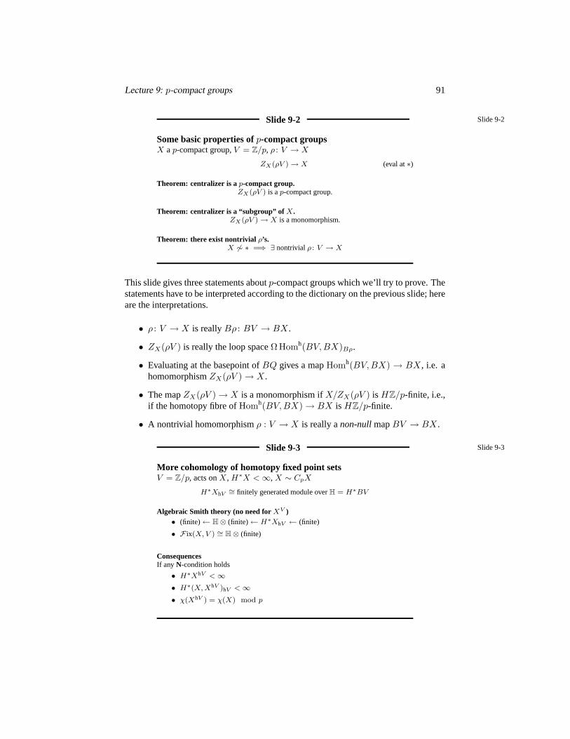
Lecture 9: p-compact groups 91
Slide 9-2 Slide 9-2
Some basic properties ofp-compact groupsX ap-compact group,V = Z/p, ρ : V → X
ZX(ρV )→ X (eval at∗)
Theorem: centralizer is ap-compact group.ZX(ρV ) is ap-compact group.
Theorem: centralizer is a “subgroup” of X.ZX(ρV )→ X is a monomorphism.
Theorem: there exist nontrivial ρ’s.X 6∼ ∗ =⇒ ∃ nontrivialρ : V → X
This slide gives three statements aboutp-compact groups which we’ll try to prove. Thestatements have to be interpreted according to the dictionary on the previous slide; hereare the interpretations.
• ρ : V → X is reallyBρ : BV → BX.
• ZX(ρV ) is really the loop spaceΩ Homh(BV,BX)Bρ.
• Evaluating at the basepoint ofBQ gives a mapHomh(BV, BX) → BX, i.e. ahomomorphismZX(ρV )→ X.
• The mapZX(ρV )→ X is a monomorphism ifX/ZX(ρV ) is HZ/p-finite, i.e.,if the homotopy fibre ofHomh(BV,BX)→ BX is HZ/p-finite.
• A nontrivial homomorphismρ : V → X is really anon-nullmapBV → BX.
Slide 9-3 Slide 9-3
More cohomology of homotopy fixed point setsV = Z/p, acts onX, H∗X < ∞, X ∼ CpX
H∗XhV∼= finitely generated module overH = H∗BV
Algebraic Smith theory (no need forXV )• (finite)← H⊗ (finite)← H∗XhV ← (finite)
• F ix(X, V ) ∼= H⊗ (finite)
ConsequencesIf any N-condition holds
• H∗XhV <∞• H∗(X, XhV )hV <∞• χ(XhV ) = χ(X) mod p

Lecture 9: p-compact groups 92
This slide deals with the situation in whichX is a p-complete space (X ∼ CpX),H∗X is finite (denotedH∗X < ∞), andV ∼= Z/p acts onX. The main referencesare [46] [47] and [64]. The first remark is that the cohomology of the homotopy orbitspaceXhV is in this case a finitely generated module overH.
? 9.6 Exercise. Prove this (probably by using the Serre spectral sequence and thefact thatH is a noetherian ring).
Of course,H∗XhV is also a module over the Steenrod algebra in a way that’s com-patible with theH-module structure. Algebraic Smith theory says that in this situationthere is always a finite algebraR overAp, and a map
H∗XhV → H⊗R
with finite kernel and cokernel. As in slides 7–2 and 7–3, this implies that if someN-condition holds,H∗XhV ∼= R. By naturality the mapH∗XhV → H∗(XhV )hV isthen the above mapH∗XhV → H⊗ R, and so the relative homologyH∗(X, XhV )hV
is finite.
Remark. Algebraic Smith theory is actually a little more explicit. LetS ⊂ H bethe multiplicative subset generated by a nonzero element in degree2 (if p = 2, let Sbe the multiplicative subset generated by the unique non-zero element of degree 1).Then S−1H∗XhV admits a natural action ofAp which is not necessarily unstable.Let Un(S−1H∗XhV ) be the maximal unstable submodule. Algebraic Smith theoryguarantees that this object splits as a tensor product
Un(S−1H∗XhV ) ∼= H⊗R
for somefiniteAp-algebraR, and the natural map
H∗XhV → H⊗R
becomes an isomorphism whenS−1(−) is applied. IfX is a genuine finite complexwith a cellular action ofV , thenR ∼= H∗XV . So in geometric situationsR is thecohomology of the fixed point set, and in homotopy theoretic situations a candidatefor the cohomology of the homotopy fixed point set. In the geometric settingXV isa volunteer forXhV (6–11), hence giving result at the bottom of 7–3. In the purelyhomotopy theoretic setting of the current slide there are usually no volunteers, and wehave to rely onN-conditions to extract information fromT .
Suppose that(X, A) is a pair of spaces, thatf : Y → X is a principalV -covering, andthatB = f−1A. Suppose in addition thatH∗(X, A) andH∗(Y, B) are finite.
? 9.7 Exercise.Prove thatχ(Y, B) = pχ(X, A). Hereχ(X, A) for instance is thealternating sum of the ranks of the modp homology groups of(X, A). (Use the fact thatif I is the augmentation ideal of the group ringFp[V ], thenIp = 0 andIk/Ik+1 ∼= Z/pfor k < p. Stitch together many long exact twisted cohomology sequences.) Deducethe final congruence on the slide.

Lecture 9: p-compact groups 93
Slide 9-4 Slide 9-4
The centralizer of V in X is ap-compact group.V = Z/p, ρ : V → X
Formula for ZX(ρV ) ΛBX = Homh(S1, BX)
ZX(ρV ) ∼
ΛBX
BV
Bρ//
;;ww
ww
BX
∼
Bρ∗ΛBX
BV
]]
4
∼ XhV
Algebraic Smith theory N-condition: XhV is anH-spaceH∗XhV <∞
End game Z = ZX(ρV )BX p-complete =⇒ BX p-local =⇒ BZ p-local+ π0Z finite =⇒ π1BZ a finitep-group=⇒ BZ p-good,p-complete
The slide begins by describingZX(ρV ) = Ω Homh(BV,BZ)Bρ as the space of liftsof Bρ into the free loop fibration overBX or equivalently the space of sections of apullback fibration overBV with X. This in turn can be interpreted the homotopy fixedpoint set of a suitable action ofV onX. As in 7.8, this is a conjugation action.
It follows from algebraic Smith theory thatH∗XhV ∼= H∗ZX(ρV ) is finite. One ofthe N-conditions is automatically satisfied, sinceXhV is anH-space, in fact a loopspace. In proving thatZX(ρV ) is a p-compact group, the end game is showing thatBZX(ρV ) is p-complete.
9.8 Exercise.Work out the “end game” reasoning sketched on the slide.
Slide 9-5 Slide 9-5
The centralizer of V in X is a subgroupV = Z/p, ρ : V → X, Z = ZX(ρV )
Construction of X/Z: V acts onBXp by permutation.
Xp/X //_
(−)hV
BXdiag //
_
(−)hV
BXp_
(−)hV
‘ρ X/Zρ ∼ (Xp/X)hV // ‘
ρ BZρ // BX
H∗(‘
ρX/Zρ) <∞ by algebraic Smith theoryN-condition:
X/Zρ // BZρ // BX =⇒‘
ρ X/Zρ is p-complete
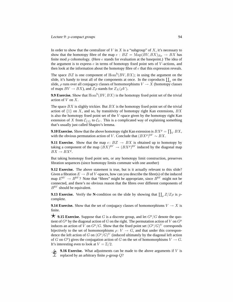
Lecture 9: p-compact groups 94
In order to show that the centralizer ofV in X is a “subgroup” ofX, it’s necessary toshow that the homotopy fibre of the mape : BZ = Map(BV, BX)Bρ → BX hasfinite modp cohomology. (Heree stands for evaluation at the basepoint.) The idea ofthe argument is to expresse in terms of homotopy fixed point sets ofV -actions, andthen look at the information about the homotopy fibre ofe that this expression reveals.
The spaceBZ is one component ofHomh(BV, BX); in using the argument on theslide, it’s handy to treat all of the components at once. In the coproducts
∐ρ on the
slide,ρ runs over all conjugacy classes of homomorphismsV → X (homotopy classesof mapsBV → BX), andZρ stands forZX(ρV ).
9.9 Exercise.Show thatHomh(BV,BX) is the homotopy fixed point set of the trivialaction ofV onX.
The spaceBX is slighly trickier. ButBX is the homotopy fixed point set of the trivialaction of1 on X, and so, by transitivity of homotopy right Kan extensions,BXis also the homotopy fixed point set of theV -space given by the homotopy right Kanextension ofX from C1 to CV . This is a complicated way of explaining somethingthat’s usually just called Shapiro’s lemma.
9.10 Exercise.Show that the above homotopy right Kan extension isBXp =∏
V BX,with the obvious permutation action ofV . Conclude that(BXp)hV ∼ BX.
9.11 Exercise. Show that the mape : BZ → BX is obtained up to homotopy bytaking a component of the map(BX)hV → (BXp)hV induced by the diagonal mapBX → BXp.
But taking homotopy fixed point sets, or any homotopy limit construction, preservesfibration sequences (since homotopy limits commute with one another)
9.12 Exercise. The above statement is true, but is it actually relevant to this slide?Given a fibrationE → B of V -spaces, how can you describe the fibre(s) of the inducedmapEhV → BhV ? Note that “fibres” might be appropriate, sinceBhV might not beconnected, and there’s no obvious reason that the fibres over different components ofBhV should be equivalent.
9.13 Exercise. Verify the N-condition on the slide by showing that∐
ρ Z/Zρ is p-complete.
9.14 Exercise.Show that the set of conjugacy classes of homomorphismsV → X isfinite.
? 9.15 Exercise.Suppose thatG is a discrete group, and letGp/G denote the quo-tient ofGp by the diagonal action ofG on the right. The permutation action ofV onGp
induces an action ofV onGp/G. Show that the fixed point set(Gp/G)V correspondsbijectively to the set of homomorphismsρ : V → G, and that under this correspon-dence the left action ofG on (Gp/G)V (induced ultimately by the diagonal left actionof G onGp) gives the conjugation action ofG on the set of homomorphismsV → G.It’s interesting even to look atV = Z/2.
9.16 Exercise.What adjustments can be made to the above arguments ifV isreplaced by an arbitrary finitep-groupQ?
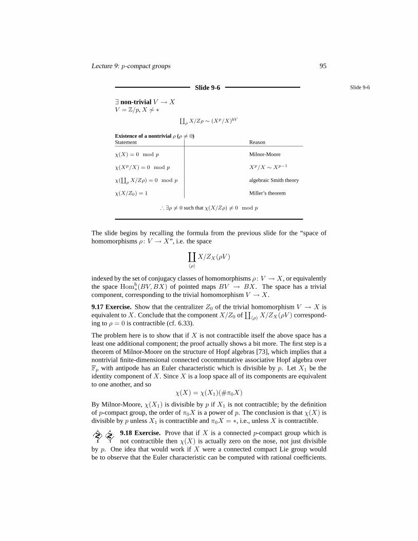
Lecture 9: p-compact groups 95
Slide 9-6 Slide 9-6
∃ non-trivial V → XV = Z/p, X 6∼ ∗ ‘
ρ X/Zρ ∼ (Xp/X)hV
Existence of a nontrivialρ (ρ 6= 0)Statement Reason
χ(X) = 0 mod p Milnor-Moore
χ(Xp/X) = 0 mod p Xp/X ∼ Xp−1
χ(‘
ρ X/Zρ) = 0 mod p algebraic Smith theory
χ(X/Z0) = 1 Miller’s theorem
∴ ∃ρ 6= 0 such thatχ(X/Zρ) 6= 0 mod p
The slide begins by recalling the formula from the previous slide for the “space ofhomomorphismsρ : V → X”, i.e. the space∐
〈ρ〉
X/ZX(ρV )
indexed by the set of conjugacy classes of homomorphismsρ : V → X, or equivalentlythe spaceHomh
∗(BV, BX) of pointed mapsBV → BX. The space has a trivialcomponent, corresponding to the trivial homomorphismV → X.
9.17 Exercise.Show that the centralizerZ0 of the trivial homomorphismV → X isequivalent toX. Conclude that the componentX/Z0 of
∐〈ρ〉 X/ZX(ρV ) correspond-
ing toρ = 0 is contractible (cf. 6.33).
The problem here is to show that ifX is not contractible itself the above space has aleast one additional component; the proof actually shows a bit more. The first step is atheorem of Milnor-Moore on the structure of Hopf algebras [73], which implies that anontrivial finite-dimensional connected cocommutative associative Hopf algebra overFp with antipode has an Euler characteristic which is divisible byp. Let X1 be theidentity component ofX. SinceX is a loop space all of its components are equivalentto one another, and so
χ(X) = χ(X1)(#π0X)
By Milnor-Moore, χ(X1) is divisible byp if X1 is not contractible; by the definitionof p-compact group, the order ofπ0X is a power ofp. The conclusion is thatχ(X) isdivisible byp unlessX1 is contractible andπ0X = ∗, i.e., unlessX is contractible.
9.18 Exercise. Prove that ifX is a connectedp-compact group which isnot contractible thenχ(X) is actually zero on the nose, not just divisible
by p. One idea that would work ifX were a connected compact Lie group wouldbe to observe that the Euler characteristic can be computed with rational coefficients.
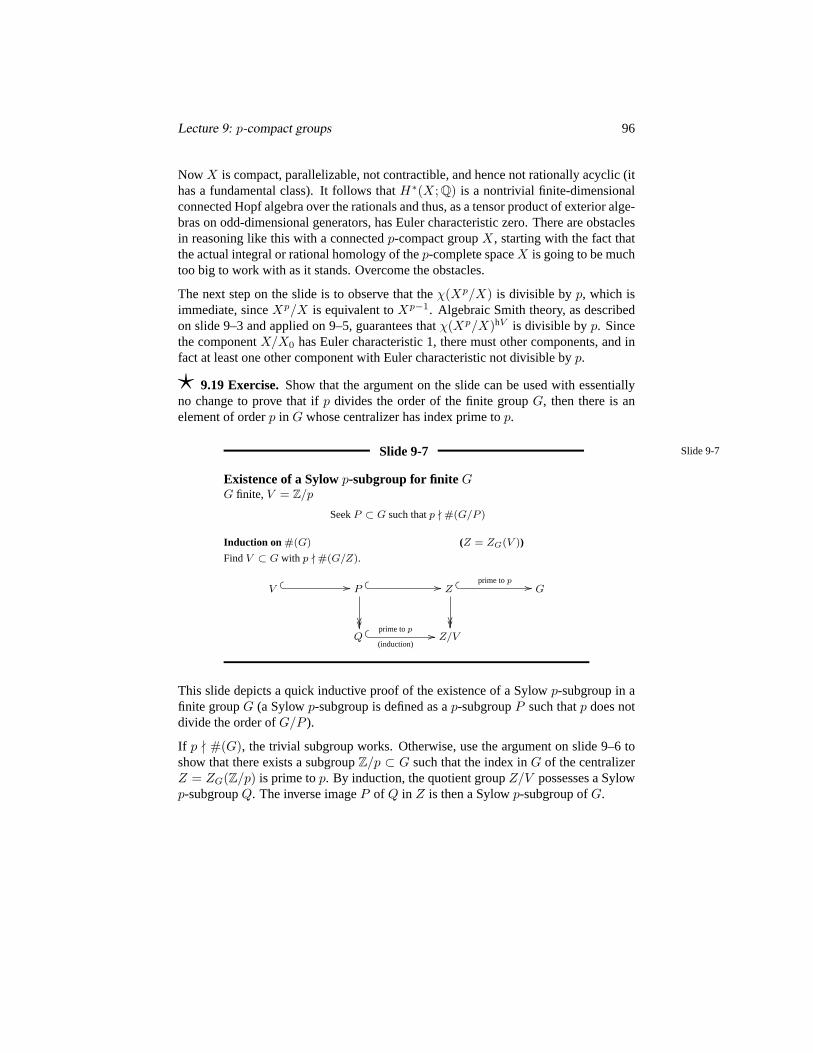
Lecture 9: p-compact groups 96
Now X is compact, parallelizable, not contractible, and hence not rationally acyclic (ithas a fundamental class). It follows thatH∗(X; Q) is a nontrivial finite-dimensionalconnected Hopf algebra over the rationals and thus, as a tensor product of exterior alge-bras on odd-dimensional generators, has Euler characteristic zero. There are obstaclesin reasoning like this with a connectedp-compact groupX, starting with the fact thatthe actual integral or rational homology of thep-complete spaceX is going to be muchtoo big to work with as it stands. Overcome the obstacles.
The next step on the slide is to observe that theχ(Xp/X) is divisible byp, which isimmediate, sinceXp/X is equivalent toXp−1. Algebraic Smith theory, as describedon slide 9–3 and applied on 9–5, guarantees thatχ(Xp/X)hV is divisible byp. Sincethe componentX/X0 has Euler characteristic 1, there must other components, and infact at least one other component with Euler characteristic not divisible byp.
? 9.19 Exercise.Show that the argument on the slide can be used with essentiallyno change to prove that ifp divides the order of the finite groupG, then there is anelement of orderp in G whose centralizer has index prime top.
Slide 9-7 Slide 9-7
Existence of a Sylowp-subgroup for finite GG finite, V = Z/p
SeekP ⊂ G such thatp - #(G/P )
Induction on #(G) (Z = ZG(V ))
FindV ⊂ G with p - #(G/Z).
V // P //
Z
prime top // G
Q prime top
(induction)// Z/V
This slide depicts a quick inductive proof of the existence of a Sylowp-subgroup in afinite groupG (a Sylowp-subgroup is defined as ap-subgroupP such thatp does notdivide the order ofG/P ).
If p - #(G), the trivial subgroup works. Otherwise, use the argument on slide 9–6 toshow that there exists a subgroupZ/p ⊂ G such that the index inG of the centralizerZ = ZG(Z/p) is prime top. By induction, the quotient groupZ/V possesses a Sylowp-subgroupQ. The inverse imageP of Q in Z is then a Sylowp-subgroup ofG.
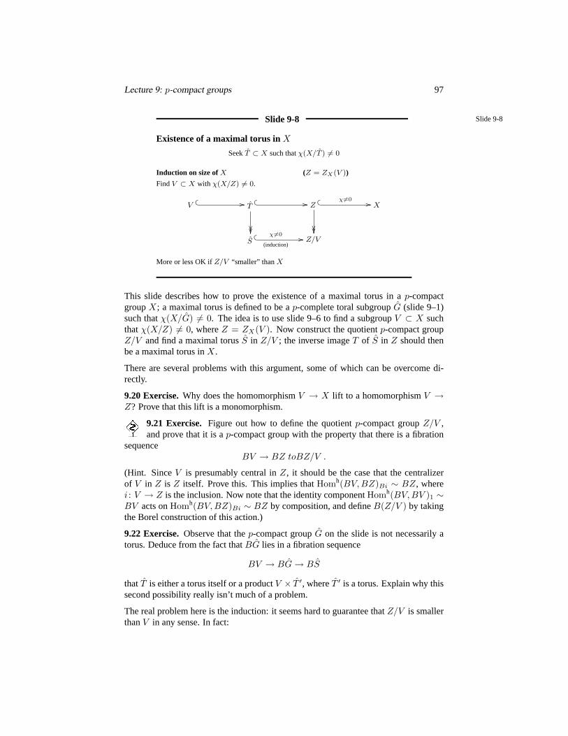
Lecture 9: p-compact groups 97
Slide 9-8 Slide 9-8
Existence of a maximal torus inX
SeekT ⊂ X such thatχ(X/T ) 6= 0
Induction on size ofX (Z = ZX(V ))
FindV ⊂ X with χ(X/Z) 6= 0.
V // T
//
Z
χ 6=0 // X
S χ 6=0
(induction)// Z/V
More or less OK ifZ/V “smaller” thanX
This slide describes how to prove the existence of a maximal torus in ap-compactgroupX; a maximal torus is defined to be ap-complete toral subgroupG (slide 9–1)such thatχ(X/G) 6= 0. The idea is to use slide 9–6 to find a subgroupV ⊂ X suchthatχ(X/Z) 6= 0, whereZ = ZX(V ). Now construct the quotientp-compact groupZ/V and find a maximal torusS in Z/V ; the inverse imageT of S in Z should thenbe a maximal torus inX.
There are several problems with this argument, some of which can be overcome di-rectly.
9.20 Exercise.Why does the homomorphismV → X lift to a homomorphismV →Z? Prove that this lift is a monomorphism.
9.21 Exercise. Figure out how to define the quotientp-compact groupZ/V ,and prove that it is ap-compact group with the property that there is a fibration
sequenceBV → BZ toBZ/V .
(Hint. SinceV is presumably central inZ, it should be the case that the centralizerof V in Z is Z itself. Prove this. This implies thatHomh(BV,BZ)Bi ∼ BZ, wherei : V → Z is the inclusion. Now note that the identity componentHomh(BV,BV )1 ∼BV acts onHomh(BV, BZ)Bi ∼ BZ by composition, and defineB(Z/V ) by takingthe Borel construction of this action.)
9.22 Exercise.Observe that thep-compact groupG on the slide is not necessarily atorus. Deduce from the fact thatBG lies in a fibration sequence
BV → BG→ BS
thatT is either a torus itself or a productV × T ′, whereT ′ is a torus. Explain why thissecond possibility really isn’t much of a problem.
The real problem here is the induction: it seems hard to guarantee thatZ/V is smallerthanV in any sense. In fact:
Lecture 9: p-compact groups 98
9.23 Exercise.Suppose thatX is a p-complete torus. Show thatZ ∼ X and (evenworse) thatZ/V ∼ X.
This problem seems like a secondary issue. . . after all, a maximal torus does exist ifXitself is a torus. Here’s one way to proceed. Assume without loss thatX is connected.
9.24 Exercise.Use Smith theory arguments (as on slide 9–6) to show thatany homomorphismZ/p → X extends to a homomorphismZ/p∞ → X.
Prove that ifZ/p → X is a monomorphism, then so isZ/p∞ → X (in the sense thatH∗X/Z/p∞ is finite).
Note thatZ/p∞ is not ap-compact group.
9.25 Exercise.Suppose thati : Z/p∞ → X is a homomorphism. Observe thatBi : BZ/p∞ → X extends overCp(BZ/p∞) → X and thatCp(BZ/p∞) ∼
K(Zp, 2) ∼ BCp(S1). Prove that ifZ/p∞ → X is a monomorphism in the senseof the previous exercise, then the induced mapCp(S1) → X is a monomorphism ofp-compact groups.
Let S = Cp(S1). We can now consider a chain of monomorphisms
V → S → ZX(S)→ ZX(V )→ X .
whereV → X has been chosen so thatχ(X/ZX(V )) 6= 0.
9.26 Exercise.What isZX(S), why is it ap-compact group, and why isZX(S)→ X a monomorphism?
9.27 Exercise.Show thatdim(ZX(S)/S) < dim X, wheredim is modpcohomological dimension. Proceed using an inductive argument to show
thatX possesses a maximal torus.
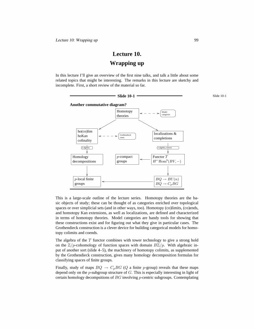
Lecture 10: Wrapping up 99
Lecture 10.
Wrapping up
In this lecture I’ll give an overview of the first nine talks, and talk a little about somerelated topics that might be interesting. The remarks in this lecture are sketchy andincomplete. First, a short review of the material so far.
Slide 10-1 Slide 10-1
Another commutative diagram?
Homotopytheories
xxqqqqqqqqqq
&&MMMMMMMMMMM
oo //_____ Model
categories
ho(co)limhoKancofinality
oo //_____
+algebra
Grothendieckconst.
localizations &completions +algebra, towers
Homologydecompositions
p-compactgroups
FunctorTH∗ Homh(BV,−)
oo
p-local finitegroups
BQ → BU(n)BQ → CpBG
oo
This is a large-scale outline of the lecture series. Homotopy theories are the ba-sic objects of study; these can be thought of as categories enriched over topologicalspaces or over simplicial sets (and in other ways, too). Homotopy (co)limits, (co)ends,and homotopy Kan extensions, as well as localizations, are defined and characterizedin terms of homotopy theories. Model categories are handy tools for showing thatthese constructions exist and for figuring out what they give in particular cases. TheGrothendieck construction is a clever device for building categorical models for homo-topy colimits and coends.
The algebra of theT functor combines with tower technology to give a strong holdon theZ/p-cohomology of function spaces with domainBZ/p. With algebraic in-put of another sort (slide 4–5), the machinery of homotopy colimits, as supplementedby the Grothendieck construction, gives many homology decomposition formulas forclassifying spaces of finite groups.
Finally, study of mapsBQ → CpBG (Q a finite p-group) reveals that these mapsdepend only on thep-subgroup structure ofG. This is especially interesting in light ofcertain homology decompsitions ofBG involving p-centric subgroups. Contemplating

Lecture 10: Wrapping up 100
these structures leads leads to a relatively simple algebraic model forCpBG. Otherspaces which can be modeled in the same way are calledp-local finite groups, andthought of as finite-group-like objects whose structure is concentrated atp.
Note: BU(n) is used on the slide as shorthand for the classifying space of a genericconnected compact Lie group.
Slide 10-2 Slide 10-2
Homotopy theories
Homotopytheories
xxqqqqqqqqqq
&&MMMMMMMMMMM
oo //_____ Model
categories
ho(co)limhoKancofinality
oo //_____
+algebra
Grothendieckconst.
localizations &completions +algebra, towers
Homologydecompositions
p-compactgroups
FunctorTH∗ Homh(BV,−)
oo
p-local finitegroups
BQ → BU(n)BQ → CpBG
oo
Higher category theory
• Homotopy theoryT = (∞, 1)-category
• Category ofT’s = (∞, 2)-category(?)
• Conformal field theories↔ (∞, n)-categories(?)
Enriched morphisms
• Spectra, chain complexes,. . .
Accepting the notion of homotopy theory is just the first step on an long and apparentlystill treacherous journey. A homotopy theory is an(∞, 1) category, a category-like ob-ject in which the morphism between two objects form a space or (if you loop down) atopological (simplicial) groupoid. The “1” in(∞, 1) refers to this groupoid quality: allof the1-morphisms are invertible. IfA andB are two homotopy categories, the mor-phism objectBhA can be constructed as a homotopy category in its own right. There’sno need for all of the maps inBhA to be invertible, but each component of a map-ping complex inBhA is an ordinary space, which via looping corresponds to groupoidobjects. To my mind (admittedly uninformed!) this signifies that the category of homo-topy theories is an(∞, 2) category. Clearly it’s possible to continue this progression. Itturns out that there is even a reason to continue: for instance,(∞, n) categories are re-lated to higher conformal field theories (think manifolds, bordisms, bordisms betweenbordisms,. . .) John Baez and Aaron Lauda have written a terrific article about thingslike this [8].
Another direction to take with homotopy theories is to introduce richer morphism ob-jects, e.g. spectra instead of spaces. For instance, Dugger and Shipley have studiedenriched model categories [31].
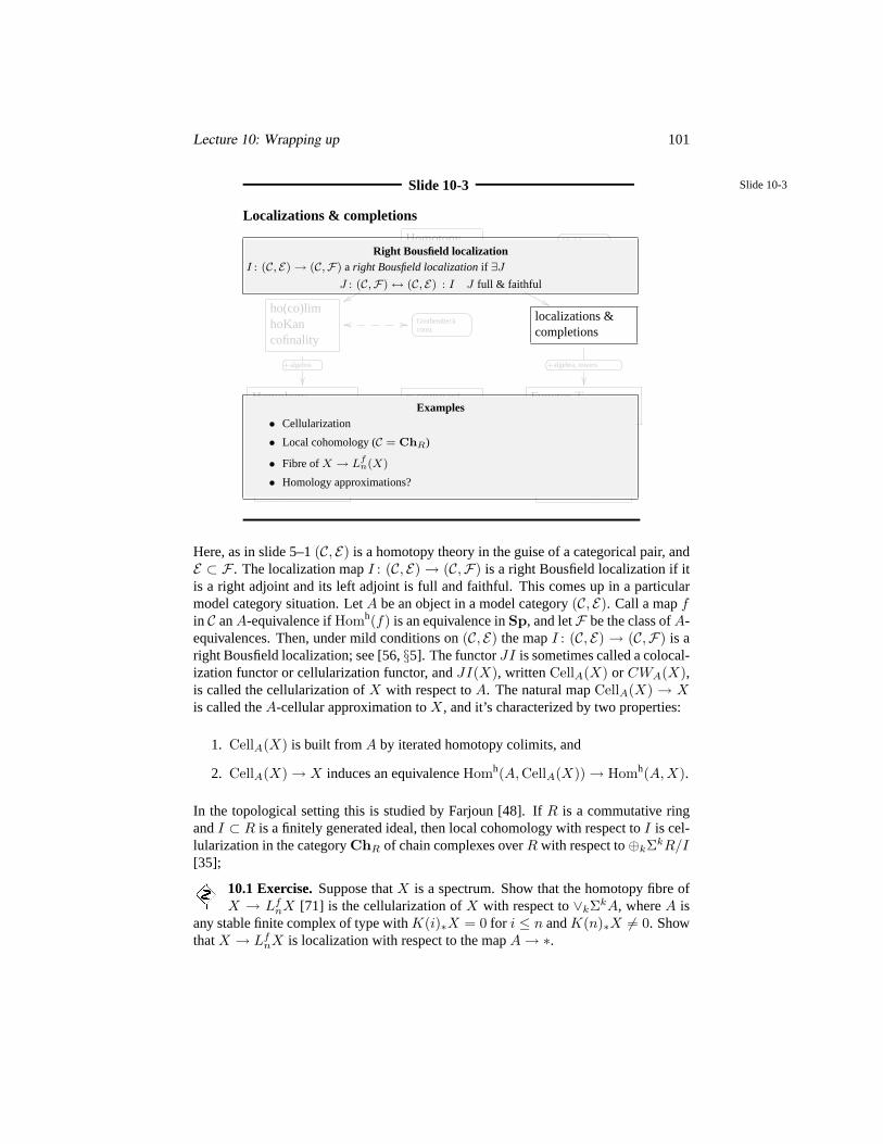
Lecture 10: Wrapping up 101
Slide 10-3 Slide 10-3
Localizations & completions
Homotopytheories
xxqqqqqqqqqq
&&MMMMMMMMMMM
oo //_____ Model
categories
ho(co)limhoKancofinality
oo //_____
+algebra
Grothendieckconst.
localizations &completions +algebra, towers
Homologydecompositions
p-compactgroups
FunctorTH∗ Homh(BV,−)
oo
p-local finitegroups
BQ → BU(n)BQ → CpBG
oo
Right Bousfield localizationI : (C, E)→ (C,F) a right Bousfield localizationif ∃J
J : (C,F)↔ (C, E) : I J full & faithful
Examples• Cellularization
• Local cohomology (C = ChR)
• Fibre ofX → Lfn(X)
• Homology approximations?
Here, as in slide 5–1(C, E) is a homotopy theory in the guise of a categorical pair, andE ⊂ F . The localization mapI : (C, E)→ (C,F) is a right Bousfield localization if itis a right adjoint and its left adjoint is full and faithful. This comes up in a particularmodel category situation. LetA be an object in a model category(C, E). Call a mapfin C anA-equivalence ifHomh(f) is an equivalence inSp, and letF be the class ofA-equivalences. Then, under mild conditions on(C, E) the mapI : (C, E) → (C,F) is aright Bousfield localization; see [56,§5]. The functorJI is sometimes called a colocal-ization functor or cellularization functor, andJI(X), writtenCellA(X) or CWA(X),is called the cellularization ofX with respect toA. The natural mapCellA(X) → Xis called theA-cellular approximation toX, and it’s characterized by two properties:
1. CellA(X) is built fromA by iterated homotopy colimits, and
2. CellA(X)→ X induces an equivalenceHomh(A,CellA(X))→ Homh(A,X).
In the topological setting this is studied by Farjoun [48]. IfR is a commutative ringandI ⊂ R is a finitely generated ideal, then local cohomology with respect toI is cel-lularization in the categoryChR of chain complexes overR with respect to⊕kΣkR/I[35];
10.1 Exercise.Suppose thatX is a spectrum. Show that the homotopy fibre ofX → Lf
nX [71] is the cellularization ofX with respect to∨kΣkA, whereA isany stable finite complex of type withK(i)∗X = 0 for i ≤ n andK(n)∗X 6= 0. ShowthatX → Lf
nX is localization with respect to the mapA→ ∗.
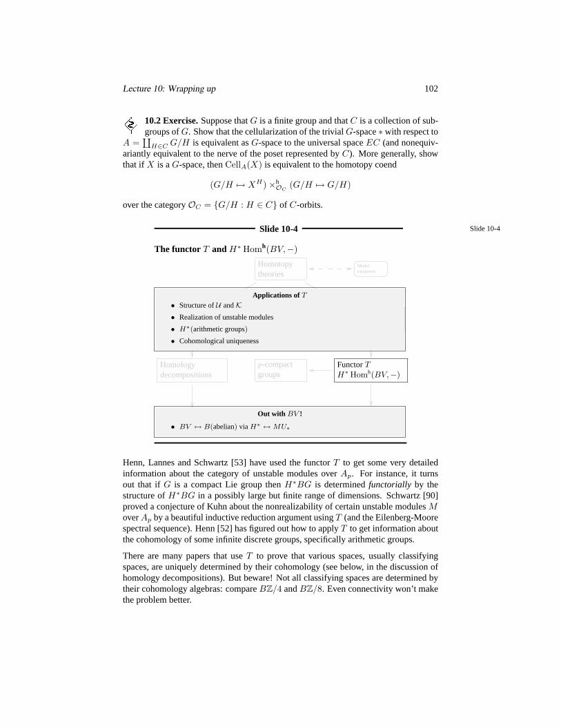
Lecture 10: Wrapping up 102
10.2 Exercise.Suppose thatG is a finite group and thatC is a collection of sub-groups ofG. Show that the cellularization of the trivialG-space∗ with respect to
A =∐
H∈C G/H is equivalent asG-space to the universal spaceEC (and nonequiv-ariantly equivalent to the nerve of the poset represented byC). More generally, showthat if X is aG-space, thenCellA(X) is equivalent to the homotopy coend
(G/H 7→ XH)×hOC
(G/H 7→ G/H)
over the categoryOC = G/H : H ∈ C of C-orbits.
Slide 10-4 Slide 10-4
The functor T and H∗ Homh(BV,−)
Homotopytheories
xxqqqqqqqqqq
&&MMMMMMMMMMM
oo //_____ Model
categories
ho(co)limhoKancofinality
oo //_____
+algebra
Grothendieckconst.
localizations &completions +algebra, towers
Homologydecompositions
p-compactgroups
FunctorTH∗ Homh(BV,−)
oo
p-local finitegroups
BQ → BU(n)BQ → CpBG
oo
Applications of T
• Structure ofU andK• Realization of unstable modules
• H∗(arithmetic groups)
• Cohomological uniqueness
Out with BV !
• BV ↔ B(abelian) via H∗ ↔MU∗
Henn, Lannes and Schwartz [53] have used the functorT to get some very detailedinformation about the category of unstable modules overAp. For instance, it turnsout that if G is a compact Lie group thenH∗BG is determinedfunctorially by thestructure ofH∗BG in a possibly large but finite range of dimensions. Schwartz [90]proved a conjecture of Kuhn about the nonrealizability of certain unstable modulesMoverAp by a beautiful inductive reduction argument usingT (and the Eilenberg-Moorespectral sequence). Henn [52] has figured out how to applyT to get information aboutthe cohomology of some infinite discrete groups, specifically arithmetic groups.
There are many papers that useT to prove that various spaces, usually classifyingspaces, are uniquely determined by their cohomology (see below, in the discussion ofhomology decompositions). But beware! Not all classifying spaces are determined bytheir cohomology algebras: compareBZ/4 andBZ/8. Even connectivity won’t makethe problem better.
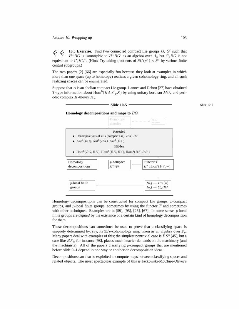
Lecture 10: Wrapping up 103
10.3 Exercise. Find two connected compact Lie groupsG, G′ such thatH∗BG is isomorphic toH∗BG′ as an algebra overAp but CpBG is not
equivalent toCpBG′. (Hint: Try taking quotients ofSU(pn) × S1 by various finitecentral subgroups.)
The two papers [2] [66] are especially fun because they look at examples in whichmore than one space (up to homotopy) realizes a given cohomology ring, and all suchrealizing spaces can be enumerated.
Suppose thatA is an abelian compact Lie group. Lannes and Dehon [27] have obtainedT -type information aboutHomh(BA,CpX) by using unitary bordismMU∗ and peri-odic complexK-theoryK∗.
Slide 10-5 Slide 10-5
Homology decompositions and maps toBG
Homotopytheories
xxqqqqqqqqqq
&&MMMMMMMMMMM
oo //_____ Model
categories
ho(co)limhoKancofinality
oo //_____
+algebra
Grothendieckconst.
localizations &completions +algebra, towers
Homologydecompositions
p-compactgroups
FunctorTH∗ Homh(BV,−)
oo
p-local finitegroups
BQ → BU(n)BQ → CpBG
oo
Revealed• Decompositions ofBG (compact Lie),BX, BF• Auth(BG), Auth(BX), Auth(BF)
Hidden
• Homh(BG, BK), Homh(BX, BY ), Homh(BF , BF ′)
Homology decompositions can be constructed for compact Lie groups,p-compactgroups, andp-local finite groups, sometimes by using the functorT and sometimeswith other techniques. Examples are in [59], [95], [25], [67]. In some sense,p-localfinite groups aredefinedby the existence of a certain kind of homology decompositionfor them.
These decompositions can sometimes be used to prove that a classifying space isuniquely determined by, say, itsZ/p-cohomology ring, taken as an algebra overFp.Many papers deal with examples of this; the simplest nontrivial case isBS3 [45], but acase likeBF4, for instance [98], places much heavier demands on the machinery (andthe machinists). All of the papers classifyingp-compact groups that are mentionedbefore slide 9–1 depend in one way or another on decomposition ideas.
Decompositions can also be exploited to compute maps between classifying spaces andrelated objects. The most spectacular example of this is Jackowski-McClure-Oliver’s
Lecture 10: Wrapping up 104
calculation of the space of self maps ofBG for G a connected compact Lie group[60]. This is not explicitly based on homology decomposition machinery, but there arehomology decompositions lurking in theG-spaces (just as homology decompositionsare derived fromG-spaces on slide 4–5). It’s possible to make similar self-equivalencecalculations forp-compact groups [6] and for fusion systems [19].
However, mapsBG → BK remain a real mystery in general; representation theoryisn’t much of a guide unlessG is a finitep-group or more generally ap-toral group.Jackowski, McClure, and Oliver have worked out some examples that show how com-plicated the situation can be [61].
10.4 Exercise.UseTV for various elementary abelian subgroupsV (not justV = Z/p) to prove that ifG is a finite group andp | #(G) then the central-
izer diagram for the collection of nontrivial elementary abelian subgroups ofG doesin fact give a homology decomposition ofBG. Working backwards, use this to obtainthe algebraic formula at the bottom of slide 4–5. Hint: Show that there is no problemwith the cohomology decomposition ifG is a finitep-group, becauseG has a centralelement of orderp and soBG itself appears in the decomposition diagram. Observethat if P is a Sylowp-subgroup ofG, then the transfer expressesH∗BG as a retract ofH∗BP . Since the cohomology of the centralizer of an elementary abelian subgroupVof G is obtained by applyingTV to H∗BG, it should follow that in some sense yet tobe determined the cohomology of the centralizer diagram forBG should be a retract ofthe cohomology of the centralizer diagram forBP and so the putative cohomologicaldecomposition arrow forBG should be a retract of the arrow forBP . But the arrowfor BP is an isomorphism, and a retract of an isomorphism is an isomorphism. KenBrown’s algebra is easier! But this kind of argument does lead to homology decompo-sitions for compact Lie groups,p-compact groups, andp-local finite groups.
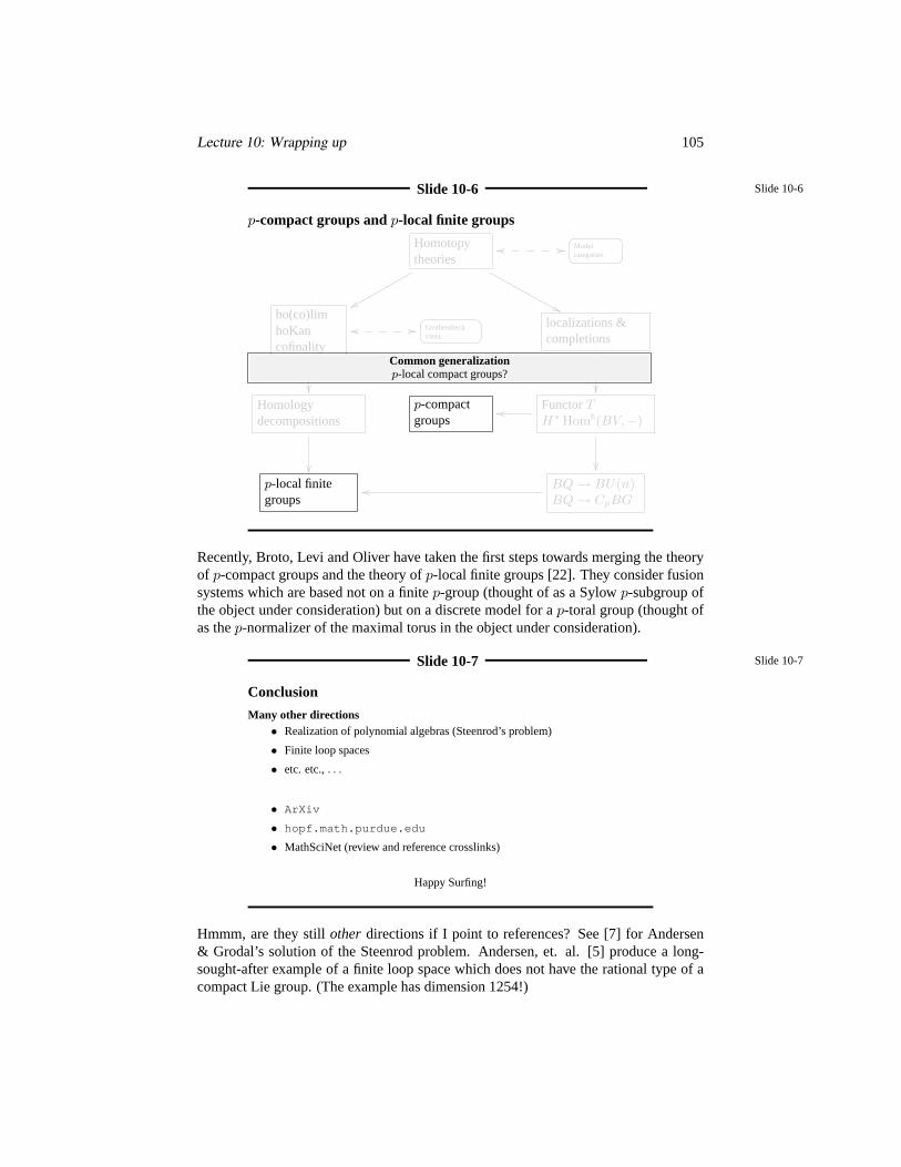
Lecture 10: Wrapping up 105
Slide 10-6 Slide 10-6
p-compact groups andp-local finite groups
Homotopytheories
xxqqqqqqqqqq
&&MMMMMMMMMMM
oo //_____ Model
categories
ho(co)limhoKancofinality
oo //_____
+algebra
Grothendieckconst.
localizations &completions +algebra, towers
Homologydecompositions
p-compactgroups
FunctorTH∗ Homh(BV,−)
oo
p-local finitegroups
BQ → BU(n)BQ → CpBG
oo
Common generalizationp-local compact groups?
Recently, Broto, Levi and Oliver have taken the first steps towards merging the theoryof p-compact groups and the theory ofp-local finite groups [22]. They consider fusionsystems which are based not on a finitep-group (thought of as a Sylowp-subgroup ofthe object under consideration) but on a discrete model for ap-toral group (thought ofas thep-normalizer of the maximal torus in the object under consideration).
Slide 10-7 Slide 10-7
Conclusion
Many other directions• Realization of polynomial algebras (Steenrod’s problem)
• Finite loop spaces
• etc. etc.,. . .
• ArXiv
• hopf.math.purdue.edu
• MathSciNet (review and reference crosslinks)
Happy Surfing!
Hmmm, are they stillother directions if I point to references? See [7] for Andersen& Grodal’s solution of the Steenrod problem. Andersen, et. al. [5] produce a long-sought-after example of a finite loop space which does not have the rational type of acompact Lie group. (The example has dimension 1254!)

Lecture 10: Wrapping up 106
References
[1] A. Adem and R. J. Milgram,Cohomology of finite groups, second ed.,Grundlehren der Mathematischen Wissenschaften [Fundamental Principles ofMathematical Sciences], vol. 309, Springer-Verlag, Berlin, 2004.
[2] J. Aguade, C. Broto, and D. Notbohm,Homotopy classification of spaces withinteresting cohomology and a conjecture of Cooke. I, Topology33 (1994), no. 3,455–492.
[3] K. K. S. Andersen and J. Grodal,The classification of 2-compact groups,Preprint. (arXiv:math.AT/0611437).
[4] K. K. S. Andersen, J. Grodal, J. M. Møller, and A. Viruel,The classification ofp-compact groups forp odd, Ann. of Math. (2)167(2008), no. 1, 95–210.
[5] K. K. S. Andersen, T. Bauer, J. Grodal, and E. K. Pedersen,A finite loop spacenot rationally equivalent to a compact Lie group, Invent. Math.157 (2004),no. 1, 1–10.
[6] K. K. S. Andersen and J. Grodal,Automorphisms ofp-compact groups and theirroot data, math.AT/0510179 .
[7] , The Steenrod problem of realizing polynomial cohomology rings,arXiv:0704.4002 .
[8] J. Baez and A. Lauda,A prehistory ofn-categorical physics, to appear inproceedings ofDeep Beauty: Mathematical Innovation and the Search foran Underlying Intelligibility of the Quantum World,ed. Hans Halvorson,http://math.ucr.edu/home/baez/history.pdf .
[9] J. E. Bergner,A model category structure on the category of simplicial cate-gories, Trans. Amer. Math. Soc.359(2007), no. 5, 2043–2058 (electronic).
[10] , Simplicial monoids and Segal categories, Categories in algebra, geom-etry and mathematical physics, Contemp. Math., vol. 431, Amer. Math. Soc.,Providence, RI, 2007, pp. 59–83.
[11] , Three models for the homotopy theory of homotopy theories, Topology46 (2007), no. 4, 397–436.
[12] A. K. Bousfield,The localization of spaces with respect to homology, Topology14 (1975), 133–150.
[13] , The localization of spectra with respect to homology, Topology 18(1979), no. 4, 257–281.
[14] , Homotopy spectral sequences and obstructions, Israel J. Math.66(1989), no. 1-3, 54–104.

Lecture 10: Wrapping up 107
[15] , On thep-adic completions of nonnilpotent spaces, Trans. Amer. Math.Soc.331(1992), no. 1, 335–359.
[16] , Homotopical localizations of spaces, Amer. J. Math.119(1997), no. 6,1321–1354.
[17] A. K. Bousfield and V. K. A. M. Gugenheim,OnPL de Rham theory and ratio-nal homotopy type, Mem. Amer. Math. Soc.8 (1976), no. 179, ix+94.
[18] A. K. Bousfield and D. M. Kan,Homotopy limits, completions and localizations,Springer-Verlag, Berlin, 1972, Lecture Notes in Mathematics, Vol. 304.
[19] C. Broto, R. Levi, and B. Oliver,Homotopy equivalences ofp-completed classi-fying spaces of finite groups, Invent. Math.151(2003), no. 3, 611–664.
[20] , The homotopy theory of fusion systems, J. Amer. Math. Soc.16 (2003),no. 4, 779–856 (electronic).
[21] , The theory ofp-local groups: a survey, Homotopy theory: relationswith algebraic geometry, group cohomology, and algebraicK-theory, Contemp.Math., vol. 346, Amer. Math. Soc., Providence, RI, 2004, pp. 51–84.
[22] , Discrete models for thep-local homotopy theory of compact Lie groupsandp-compact groups, Geom. Topol.11 (2007), 315–427.
[23] S. R. Bullett and I. G. Macdonald,On the Adem relations, Topology21 (1982),no. 3, 329–332.
[24] C. Casacuberta, D. Scevenels, and J. H. Smith,Implications of large-cardinalprinciples in homotopical localization, Adv. Math.197(2005), no. 1, 120–139.
[25] N. Castellana, R. Levi, and D. Notbohm,Homology decompositions forp-compact groups, Adv. Math.216(2007), no. 2, 491–534.
[26] W. Chacholski and J. Scherer,Homotopy theory of diagrams, Mem. Amer. Math.Soc.155(2002), no. 736, x+90.
[27] F.-X. Dehon and J. Lannes,Sur les espaces fonctionnels dont la source est leclassifiant d’un groupe de Lie compact commutatif, Inst. HautesEtudes Sci.Publ. Math. (1999), no. 89, 127–177 (2000).
[28] E. Dror, W. G. Dwyer, and D. M. Kan,Equivariant maps which are self homo-topy equivalences, Proc. Amer. Math. Soc.80 (1980), no. 4, 670–672.
[29] E. Dror Farjoun and J. Smith,A geometric interpretation of Lannes’ functorT,Asterisque (1990), no. 191, 6, 87–95, International Conference on HomotopyTheory (Marseille-Luminy, 1988).
[30] D. Dugger and D. C. Isaksen,Topological hypercovers andA1-realizations,Math. Z.246(2004), no. 4, 667–689.
Lecture 10: Wrapping up 108
[31] D. Dugger and B. Shipley,Enriched model categories and an application toadditive endomorphism spectra, Theory Appl. Categ.18 (2007), No. 15, 400–439 (electronic).
[32] W. Dwyer and A. Zabrodsky,Maps between classifying spaces, Algebraic topol-ogy, Barcelona, 1986, Lecture Notes in Math., vol. 1298, Springer, Berlin, 1987,pp. 106–119.
[33] W. G. Dwyer,Homology decompositions for classifying spaces of finite groups,Topology36 (1997), no. 4, 783–804.
[34] , Sharp homology decompositions for classifying spaces of finite groups,Group representations: cohomology, group actions and topology (Seattle, WA,1996), Proc. Sympos. Pure Math., vol. 63, Amer. Math. Soc., Providence, RI,1998, pp. 197–220.
[35] W. G. Dwyer and J. P. C. Greenlees,Complete modules and torsion modules,Amer. J. Math.124(2002), no. 1, 199–220.
[36] W. G. Dwyer and D. M. Kan,Calculating simplicial localizations, J. Pure Appl.Algebra18 (1980), no. 1, 17–35.
[37] , Function complexes in homotopical algebra, Topology 19 (1980),no. 4, 427–440.
[38] , Simplicial localizations of categories, J. Pure Appl. Algebra17 (1980),no. 3, 267–284.
[39] , A classification theorem for diagrams of simplicial sets, Topology23(1984), no. 2, 139–155.
[40] , Equivalences between homotopy theories of diagrams, Algebraictopology and algebraicK-theory (Princeton, N.J., 1983), Ann. of Math. Stud.,vol. 113, Princeton Univ. Press, Princeton, NJ, 1987, pp. 180–205.
[41] W. G. Dwyer and J. Spalinski,Homotopy theories and model categories, Hand-book of algebraic topology, North-Holland, Amsterdam, 1995, pp. 73–126.
[42] W. G. Dwyer and C. W. Wilkerson,Homotopy fixed-point methods for Liegroups and finite loop spaces, Ann. of Math. (2)139(1994), no. 2, 395–442.
[43] W. G. Dwyer and H.-W. Henn,Homotopy theoretic methods in group cohomol-ogy, Advanced Courses in Mathematics. CRM Barcelona, Birkhauser Verlag,Basel, 2001.
[44] W. G. Dwyer, P. S. Hirschhorn, D. M. Kan, and J. H. Smith,Homotopy limitfunctors on model categories and homotopical categories, Mathematical Sur-veys and Monographs, vol. 113, American Mathematical Society, Providence,RI, 2004.
Lecture 10: Wrapping up 109
[45] W. G. Dwyer, H. R. Miller, and C. W. Wilkerson,The homotopic uniqueness ofBS3, Algebraic topology, Barcelona, 1986, Lecture Notes in Math., vol. 1298,Springer, Berlin, 1987, pp. 90–105.
[46] W. G. Dwyer and C. W. Wilkerson,Smith theory revisited, Ann. of Math. (2)127(1988), no. 1, 191–198.
[47] , Smith theory and the functorT , Comment. Math. Helv.66 (1991),no. 1, 1–17.
[48] E. D. Farjoun,Cellular spaces, null spaces and homotopy localization, LectureNotes in Mathematics, vol. 1622, Springer-Verlag, Berlin, 1996.
[49] P. G. Goerss and J. F. Jardine,Simplicial homotopy theory, Progress in Mathe-matics, vol. 174, Birkhauser Verlag, Basel, 1999.
[50] J. Grodal and S. D. Smith,Propagating sharp group homology decompositions,Adv. Math.200(2006), no. 2, 525–538.
[51] D. K. Harrison,Infinite abelian groups and homological methods, Ann. of Math.(2) 69 (1959), 366–391.
[52] H.-W. Henn,Unstable modules over the Steenrod algebra and cohomology ofgroups, Group representations: cohomology, group actions and topology (Seat-tle, WA, 1996), Proc. Sympos. Pure Math., vol. 63, Amer. Math. Soc., Provi-dence, RI, 1998, pp. 277–300.
[53] H.-W. Henn, J. Lannes, and L. Schwartz,Localizations of unstableA-modulesand equivariant modp cohomology, Math. Ann.301(1995), no. 1, 23–68.
[54] K. Hess,Model categories in algebraic topology, Appl. Categ. Structures10(2002), no. 3, 195–220, Papers in honour of the seventieth birthday of ProfessorHeinrich Kleisli (Fribourg, 2000).
[55] , Rational homotopy theory: a brief introduction, Interactions betweenhomotopy theory and algebra, Contemp. Math., vol. 436, Amer. Math. Soc.,Providence, RI, 2007, pp. 175–202.
[56] P. S. Hirschhorn,Model categories and their localizations, Mathematical Sur-veys and Monographs, vol. 99, American Mathematical Society, Providence, RI,2003.
[57] J. Hollender and R. M. Vogt,Modules of topological spaces, applications tohomotopy limits andE∞ structures, Arch. Math. (Basel)59 (1992), no. 2, 115–129.
[58] M. Hovey, Model categories, Mathematical Surveys and Monographs, vol. 63,American Mathematical Society, Providence, RI, 1999.
[59] S. Jackowski and J. McClure,Homotopy decomposition of classifying spaces viaelementary abelian subgroups, Topology31 (1992), no. 1, 113–132.
Lecture 10: Wrapping up 110
[60] S. Jackowski, J. McClure, and B. Oliver,Homotopy classification of self-mapsof BG via G-actions. I, Ann. of Math. (2)135(1992), no. 1, 183–226.
[61] , Maps between classifying spaces revisited, The Cech centennial(Boston, MA, 1993), Contemp. Math., vol. 181, Amer. Math. Soc., Providence,RI, 1995, pp. 263–298.
[62] A. Joyal, Quasi-categories and Kan complexes, J. Pure Appl. Algebra175(2002), no. 1-3, 207–222, Special volume celebrating the 70th birthday of Pro-fessor Max Kelly.
[63] A. Joyal and M. Tierney,Quasi-categories vs Segal spaces, Categories in al-gebra, geometry and mathematical physics, Contemp. Math., vol. 431, Amer.Math. Soc., Providence, RI, 2007, pp. 277–326.
[64] J. Lannes,Sur les espaces fonctionnels dont la source est le classifiant d’unp-groupe abelienelementaire, Inst. HautesEtudes Sci. Publ. Math. (1992), no. 75,135–244, With an appendix by Michel Zisman.
[65] , Theorie homotopique des groupes de Lie (d’apres W. G. Dwyer et C.W. Wilkerson), Asterisque (1995), no. 227, Exp. No. 776, 3, 21–45, SeminaireBourbaki, Vol. 1993/94.
[66] K. Lesh,Hybrid spaces with interesting cohomology, Trans. Amer. Math. Soc.347(1995), no. 9, 3247–3262.
[67] A. Libman, The normaliser decomposition forp-local finite groups, Algebr.Geom. Topol.6 (2006), 1267–1288 (electronic).
[68] S. Mac Lane,Categories for the working mathematician, second ed., GraduateTexts in Mathematics, vol. 5, Springer-Verlag, New York, 1998.
[69] M. A. Mandell,E∞ algebras andp-adic homotopy theory, Topology40 (2001),no. 1, 43–94.
[70] J. P. May,Simplicial objects in algebraic topology, Chicago Lectures in Math-ematics, University of Chicago Press, Chicago, IL, 1992, Reprint of the 1967original.
[71] H. Miller, Finite localizations, Bol. Soc. Mat. Mexicana (2)37 (1992), no. 1-2,383–389, Papers in honor of Jose Adem (Spanish).
[72] J. Milnor,The Steenrod algebra and its dual, Ann. of Math. (2)67 (1958), 150–171.
[73] J. W. Milnor and J. C. Moore,On the structure of Hopf algebras, Ann. of Math.(2) 81 (1965), 211–264.
[74] G. Mislin, On group homomorphisms inducing mod-p cohomology isomor-phisms, Comment. Math. Helv.65 (1990), no. 3, 454–461.
Lecture 10: Wrapping up 111
[75] J. M. Møller and D. Notbohm,Connected finite loop spaces with maximal tori,Trans. Amer. Math. Soc.350(1998), no. 9, 3483–3504.
[76] J. M. Møller,Homotopy Lie groups, Bull. Amer. Math. Soc. (N.S.)32 (1995),no. 4, 413–428.
[77] , N -determined 2-compact groups. I, Fund. Math.195 (2007), no. 1,11–84.
[78] , N -determined 2-compact groups. II, Fund. Math.196 (2007), no. 1,1–90.
[79] F. Morel, Quelques remarques sur la cohomologie modulop continue des pro-p-espaces et les resultats de J. Lannes concernant les espaces fonctionnelshom(BV,X), Ann. Sci.Ecole Norm. Sup. (4)26 (1993), no. 3, 309–360.
[80] D. Notbohm,Maps between classifying spaces, Math. Z.207(1991), no. 1, 153–168.
[81] B. Oliver, Equivalences of classifying spaces completed at odd primes, Math.Proc. Cambridge Philos. Soc.137(2004), no. 2, 321–347.
[82] , Equivalences of classifying spaces completed at the prime two, Mem.Amer. Math. Soc.180(2006), no. 848, vi+102.
[83] D. Quillen,Rational homotopy theory, Ann. of Math. (2)90 (1969), 205–295.
[84] , On the (co-) homology of commutative rings, Applications of Categor-ical Algebra (Proc. Sympos. Pure Math., Vol. XVII, New York, 1968), Amer.Math. Soc., Providence, R.I., 1970, pp. 65–87.
[85] , Higher algebraic K-theory. I, Algebraic K-theory, I: HigherK-theories (Proc. Conf., Battelle Memorial Inst., Seattle, Wash., 1972), Springer,Berlin, 1973, pp. 85–147. Lecture Notes in Math., Vol. 341.
[86] D. G. Quillen, Homotopical algebra, Lecture Notes in Mathematics, No. 43,Springer-Verlag, Berlin, 1967.
[87] D. L. Rector,Steenrod operations in the Eilenberg-Moore spectral sequence,Comment. Math. Helv.45 (1970), 540–552.
[88] , Loop structures on the homotopy type ofS3, Symposium on AlgebraicTopology (Battelle Seattle Res. Center, Seattle, Wash., 1971), Springer, Berlin,1971, pp. 99–105. Lecture Notes in Math., Vol. 249.
[89] C. Rezk,A model for the homotopy theory of homotopy theory, Trans. Amer.Math. Soc.353(2001), no. 3, 973–1007 (electronic).
[90] L. Schwartz,La filtration de Krull de la categorieU et la cohomologie desespaces, Algebr. Geom. Topol.1 (2001), 519–548 (electronic).
Lecture 10: Wrapping up 112
[91] G. Segal,Categories and cohomology theories, Topology13 (1974), 293–312.
[92] B. E. Shipley,Pro-isomorphisms of homology towers, Math. Z. 220 (1995),no. 2, 257–271.
[93] E. H. Spanier,Algebraic topology, Springer-Verlag, New York, 1981, Correctedreprint.
[94] N. E. Steenrod,Cohomology operations, Lectures by N. E. STeenrod written andrevised by D. B. A. Epstein. Annals of Mathematics Studies, No. 50, PrincetonUniversity Press, Princeton, N.J., 1962.
[95] A. Strounine,Homology decompositions for classifying spaces of compact Liegroups, Trans. Amer. Math. Soc.352(2000), no. 6, 2643–2657.
[96] D. Sullivan, Infinitesimal computations in topology, Inst. HautesEtudes Sci.Publ. Math. (1977), no. 47, 269–331 (1978).
[97] R. W. Thomason,Homotopy colimits in the category of small categories, Math.Proc. Cambridge Philos. Soc.85 (1979), no. 1, 91–109.
[98] A. Viruel, Mod 3 homotopy uniqueness ofBF4, J. Math. Kyoto Univ.41 (2001),no. 4, 769–793.
[99] P. J. Webb,A split exact sequence of Mackey functors, Comment. Math. Helv.66 (1991), no. 1, 34–69.
[100] C. Wilkerson,Classification of spaces of the samen-type for alln, Proc. Amer.Math. Soc.60 (1976), 279–285 (1977).
[101] C. W. Wilkerson, Applications of minimal simplicial groups, Topology 15(1976), no. 2, 111–130.