Embed Size (px)
Citation preview
Homogeneity in supergravity
Noel Hustler
Doctor of PhilosophyUniversity of Edinburgh
2016

Declaration
I declare that this thesis was composed by myself and that the work contained therein is my
own, except where explicitly stated otherwise in the text. Some of the work in this thesis has
been developed in collaboration with José Figueroa-O’Farrill, reported in [1, 2, 3] and with
Andree Lischewski, reported in [4]. The work has not been submitted for any other degree or
professional qualification.
(Noel Hustler)
ii
Lay summary
There are currently two pillars of modern physics that we use to describe the universe around us:
the theory of General Relativity which describes the fundamental force of gravity through the
curving geometry of spacetime; and the Standard Model, a quantum field theory which describes
all the other fundamental forces through the interactions of elementary particles. These two
theories are philosophically and physically incompatible with each other; and in the few (but
incredibly fundamental) scenarios in which we require both theories to combine in order to
model a phenomenon, they either break down, disagree with each other, or more commonly
and perversely do both at the same time. As such, we know that they must be but two different
approximations of some grander, overarching, and unified theory; our best prospect for such a
unified theory is known as string theory.
When we talk about string theory as a potential unified theory, we are actually talking about
superstring theory; that is, supersymmetric string theory. Supersymmetry is a hypothetical
symmetry between different kinds of elementary particles. If, as many people believe, the
Standard Model were supersymmetric, then for each kind of elementary particle we know of,
we would expect there to exist another particle known as its superpartner. As an example, we
know that electrons exist and so there must be some as yet undetected superpartner particle
we will call selectrons. Quarks must mean there exist squarks, photons mean photinos, Higgs
bosons mean Higgsinos — you get the idea.
It can be quite difficult to calculate the things that we want to in string theory and so very
often we will look at an approximation to string theory in which we ignore some of the more
fiddly effects; such an approximation we call a theory of supergravity. String theory and thus
supergravity must by necessity contain fundamental aspects of both General Relativity and
supersymmetric quantum field theory and so solutions to a theory of supergravity have both
the curving geometry of spacetime and fundamental particles with supersymmetry. This thesis
draws a deep connection between the amount of supersymmetry that a supergravity solution
has and how homogeneous (or simple) the solution’s spacetime geometry must be. The theme
of this connection is that the more supersymmetry we have, the simpler the spacetime geometry.
iii
Abstract
This thesis is divided into three main parts. In the first of these (comprising chapters 1 and 2)
we present the physical context of the research and cover the basic geometric background we
will need to use throughout the rest of this thesis.
In the second part (comprising chapters 3 to 5) we motivate and develop the strong homo-
geneity theorem for supergravity backgrounds. We go on to prove it directly for a number of
top-dimensional Poincaré supergravities and furthermore demonstrate how it also generically
applies to dimensional reductions of those theories.
In the third part (comprising chapters 6 and 7) we show how further specialising to the case
of symmetric backgrounds allows us to compute complete classifications of such backgrounds.
We demonstrate this by classifying all symmetric type IIB supergravity backgrounds. Next we
apply an algorithm for computing the supersymmetry of symmetric backgrounds and use this to
classify all supersymmetric symmetric M-theory backgrounds.
iv
Acknowledgements
I would first and foremost like to thank my supervisor, José Figueroa-O’Farrill for the privilege
of his time and tutelage, company and friendship. His transfinite patience and passion for
explanation and demonstration have been a Richard Parker alike force during my PhD. I’m
unsure if his voluminous knowledge of and intuition for mathematical physics are more inspiring
or terrifying; certainly the former when he’s in full flow and perhaps leaning towards the latter
when one tries to then reverse engineer his manoeuvres. Actually, forget that, he’s just damn
inspiring and I’m wide-eyed whenever he winds up to pitch. Thanks José!
I’d like to thank my mother who has always been there for me and if this be the verse,
embodies its obverse. I’m also indebted to Vernon Levy and Chris Patti, two teachers who
believed in me from early on. The whole EMPG group has been magnificent and I’d like to thank
in particular: Joan Simon, James Lucietti, Harry Braden, and Christian Saemann. A special
mention for Gill Law of the Edinburgh School of Mathematics, who has been a rock. I’d also like
to thank the EPSRC for financing this Borgesian conundrum.
I’ve been supported by many friends, old and new, and although many of them were a
convenient excuse not to work as much as I should have, they have all kept me sane-ish, and
fed my soul in any number of ways. In particular, and ordered by ability to balance a ping-pong
ball on their nose, I would like to thank: Amy Wilson, Hari Sriskantha, Daniele Sepe, Tim
Roads, Elvia Rivera de la Cruz, Patricia Ritter, Paul Reynolds, Gideon Reid, Patrick Orson, Karen
Ogilvie, Raneem Mourad, Paul de Medeiros, Andree Lischewski, Monika Krol, George Kinnear,
Jonathan Hickman, Eric Hall, Lisa Glaser, Moustafa Gharamti, Michael Down, Barry Devlin,
Conor Cusack, Asa Cusack, Tim Candy, Tibor Antal, and Spiros Adams-Florou. Yes, you’re right,
that was actually reverse alphabetical order; I just couldn’t collect the data in time.
v

The stage is too big for the drama.
vi
Contents
Lay summary iii
Abstract iv
Acknowledgements v
Contents vii
1 Introduction 1
1.1 Fundamentals . . . . . . . . . . . . . . . . . . . . . . . . . . . . . . . . . . . . . . 1
1.2 General Relativity . . . . . . . . . . . . . . . . . . . . . . . . . . . . . . . . . . . . 1
1.3 The Standard Model . . . . . . . . . . . . . . . . . . . . . . . . . . . . . . . . . . 1
1.4 Supersymmetry . . . . . . . . . . . . . . . . . . . . . . . . . . . . . . . . . . . . . 2
1.5 Supergravity . . . . . . . . . . . . . . . . . . . . . . . . . . . . . . . . . . . . . . 3
1.6 String theory . . . . . . . . . . . . . . . . . . . . . . . . . . . . . . . . . . . . . . 3
1.7 Back to supergravity . . . . . . . . . . . . . . . . . . . . . . . . . . . . . . . . . . 4
2 Homogeneity 5
2.1 Homogeneous spaces . . . . . . . . . . . . . . . . . . . . . . . . . . . . . . . . . . 5
2.1.1 Homogeneity . . . . . . . . . . . . . . . . . . . . . . . . . . . . . . . . . . 5
2.1.2 Coset manifolds . . . . . . . . . . . . . . . . . . . . . . . . . . . . . . . . . 5
2.1.3 Reductive homogeneous spaces . . . . . . . . . . . . . . . . . . . . . . . . 7
2.1.4 (Pseudo-)Riemannian homogeneous spaces . . . . . . . . . . . . . . . . . 8
2.1.5 Locally homogeneous spaces . . . . . . . . . . . . . . . . . . . . . . . . . 8
2.2 Symmetric spaces . . . . . . . . . . . . . . . . . . . . . . . . . . . . . . . . . . . . 8
2.2.1 Definition . . . . . . . . . . . . . . . . . . . . . . . . . . . . . . . . . . . . 8
2.2.2 Lorentzian symmetric spaces . . . . . . . . . . . . . . . . . . . . . . . . . 9
3 The homogeneity theorem 12
3.1 Introduction . . . . . . . . . . . . . . . . . . . . . . . . . . . . . . . . . . . . . . . 12
3.2 Killing vectors . . . . . . . . . . . . . . . . . . . . . . . . . . . . . . . . . . . . . . 12
3.2.1 Working at a point . . . . . . . . . . . . . . . . . . . . . . . . . . . . . . . 13
3.2.2 Supergravity Killing vectors . . . . . . . . . . . . . . . . . . . . . . . . . . 14
3.3 Killing spinors . . . . . . . . . . . . . . . . . . . . . . . . . . . . . . . . . . . . . . 14
vii
3.3.1 Working at a point . . . . . . . . . . . . . . . . . . . . . . . . . . . . . . . 15
3.3.2 Supersymmetry . . . . . . . . . . . . . . . . . . . . . . . . . . . . . . . . . 15
3.4 The Killing superalgebra . . . . . . . . . . . . . . . . . . . . . . . . . . . . . . . . 16
3.4.1 Lie superalgebras . . . . . . . . . . . . . . . . . . . . . . . . . . . . . . . . 16
3.4.2 The symmetry superalgebra . . . . . . . . . . . . . . . . . . . . . . . . . . 16
3.4.3 The Killing superalgebra . . . . . . . . . . . . . . . . . . . . . . . . . . . . 21
3.5 The theorem . . . . . . . . . . . . . . . . . . . . . . . . . . . . . . . . . . . . . . 21
3.5.1 Motivation . . . . . . . . . . . . . . . . . . . . . . . . . . . . . . . . . . . 21
3.5.2 Working at a point . . . . . . . . . . . . . . . . . . . . . . . . . . . . . . . 22
3.5.3 Proof . . . . . . . . . . . . . . . . . . . . . . . . . . . . . . . . . . . . . . 22
3.5.4 Summary . . . . . . . . . . . . . . . . . . . . . . . . . . . . . . . . . . . . 24
4 Application of the theorem 26
4.1 Introduction . . . . . . . . . . . . . . . . . . . . . . . . . . . . . . . . . . . . . . . 26
4.2 D = 11 . . . . . . . . . . . . . . . . . . . . . . . . . . . . . . . . . . . . . . . . . . 26
4.2.1 Introduction . . . . . . . . . . . . . . . . . . . . . . . . . . . . . . . . . . . 26
4.2.2 Conventions . . . . . . . . . . . . . . . . . . . . . . . . . . . . . . . . . . . 26
4.2.3 Definition . . . . . . . . . . . . . . . . . . . . . . . . . . . . . . . . . . . . 26
4.2.4 Spinor representation . . . . . . . . . . . . . . . . . . . . . . . . . . . . . 27
4.2.5 Spinor inner product . . . . . . . . . . . . . . . . . . . . . . . . . . . . . . 27
4.2.6 Almost Killing superalgebra and homogeneity . . . . . . . . . . . . . . . . 27
4.2.7 Killing superalgebra . . . . . . . . . . . . . . . . . . . . . . . . . . . . . . 29
4.3 D = 10 type IIB . . . . . . . . . . . . . . . . . . . . . . . . . . . . . . . . . . . . . 29
4.3.1 Introduction . . . . . . . . . . . . . . . . . . . . . . . . . . . . . . . . . . . 29
4.3.2 Conventions . . . . . . . . . . . . . . . . . . . . . . . . . . . . . . . . . . . 29
4.3.3 Definition . . . . . . . . . . . . . . . . . . . . . . . . . . . . . . . . . . . . 29
4.3.4 Spinor representation . . . . . . . . . . . . . . . . . . . . . . . . . . . . . 30
4.3.5 Spinor inner product . . . . . . . . . . . . . . . . . . . . . . . . . . . . . . 31
4.3.6 Almost Killing superalgebra and homogeneity . . . . . . . . . . . . . . . . 31
4.4 D = 10 type I/heterotic . . . . . . . . . . . . . . . . . . . . . . . . . . . . . . . . 32
4.4.1 Introduction . . . . . . . . . . . . . . . . . . . . . . . . . . . . . . . . . . . 32
4.4.2 Conventions . . . . . . . . . . . . . . . . . . . . . . . . . . . . . . . . . . . 32
4.4.3 Definition . . . . . . . . . . . . . . . . . . . . . . . . . . . . . . . . . . . . 32
4.4.4 Spinor representation . . . . . . . . . . . . . . . . . . . . . . . . . . . . . 33
4.4.5 Spinor inner product . . . . . . . . . . . . . . . . . . . . . . . . . . . . . . 34
4.4.6 Almost Killing superalgebra and homogeneity . . . . . . . . . . . . . . . . 34
4.4.7 Killing superalgebra . . . . . . . . . . . . . . . . . . . . . . . . . . . . . . 36
4.5 D = 6, (1, 0) . . . . . . . . . . . . . . . . . . . . . . . . . . . . . . . . . . . . . . . 37
4.5.1 Introduction . . . . . . . . . . . . . . . . . . . . . . . . . . . . . . . . . . . 37
viii
4.5.2 Conventions . . . . . . . . . . . . . . . . . . . . . . . . . . . . . . . . . . . 38
4.5.3 Definition . . . . . . . . . . . . . . . . . . . . . . . . . . . . . . . . . . . . 38
4.5.4 Spinor representation . . . . . . . . . . . . . . . . . . . . . . . . . . . . . 38
4.5.5 Spinor inner product . . . . . . . . . . . . . . . . . . . . . . . . . . . . . . 39
4.5.6 Almost Killing superalgebra and homogeneity . . . . . . . . . . . . . . . . 39
4.5.7 Killing superalgebra . . . . . . . . . . . . . . . . . . . . . . . . . . . . . . 40
4.6 D = 6, (2, 0) . . . . . . . . . . . . . . . . . . . . . . . . . . . . . . . . . . . . . . . 41
4.6.1 Introduction . . . . . . . . . . . . . . . . . . . . . . . . . . . . . . . . . . . 41
4.6.2 Conventions . . . . . . . . . . . . . . . . . . . . . . . . . . . . . . . . . . . 41
4.6.3 Definition . . . . . . . . . . . . . . . . . . . . . . . . . . . . . . . . . . . . 42
4.6.4 Spinor representation . . . . . . . . . . . . . . . . . . . . . . . . . . . . . 42
4.6.5 Spinor inner product . . . . . . . . . . . . . . . . . . . . . . . . . . . . . . 43
4.6.6 Almost Killing superalgebra and homogeneity . . . . . . . . . . . . . . . . 43
4.6.7 Killing superalgebra . . . . . . . . . . . . . . . . . . . . . . . . . . . . . . 45
4.7 D = 4, N = 1 . . . . . . . . . . . . . . . . . . . . . . . . . . . . . . . . . . . . . . 46
4.7.1 Introduction . . . . . . . . . . . . . . . . . . . . . . . . . . . . . . . . . . . 46
4.7.2 Conventions . . . . . . . . . . . . . . . . . . . . . . . . . . . . . . . . . . . 47
4.7.3 Definition . . . . . . . . . . . . . . . . . . . . . . . . . . . . . . . . . . . . 47
4.7.4 Spinor representation . . . . . . . . . . . . . . . . . . . . . . . . . . . . . 47
4.7.5 Spinor inner product . . . . . . . . . . . . . . . . . . . . . . . . . . . . . . 47
4.7.6 Almost Killing superalgebra and homogeneity . . . . . . . . . . . . . . . . 48
4.7.7 Killing superalgebra . . . . . . . . . . . . . . . . . . . . . . . . . . . . . . 48
5 Dimensional reduction of the theorem 49
5.1 Introduction . . . . . . . . . . . . . . . . . . . . . . . . . . . . . . . . . . . . . . . 49
5.2 Dimensional reduction . . . . . . . . . . . . . . . . . . . . . . . . . . . . . . . . . 50
5.3 Decomposition of massless fields . . . . . . . . . . . . . . . . . . . . . . . . . . . 51
5.4 Decomposition of Killing spinor equations . . . . . . . . . . . . . . . . . . . . . . 53
5.4.1 D = 11 Killing spinor equations reduction . . . . . . . . . . . . . . . . . . 53
5.4.2 D = 6, (1, 0) Killing spinor equations reduction . . . . . . . . . . . . . . . 55
5.5 The homogeneity theorem for dimensional reductions . . . . . . . . . . . . . . . 57
5.6 Conclusion . . . . . . . . . . . . . . . . . . . . . . . . . . . . . . . . . . . . . . . 60
6 Symmetric type IIB supergravity backgrounds 62
6.1 Introduction . . . . . . . . . . . . . . . . . . . . . . . . . . . . . . . . . . . . . . . 62
6.2 D = 10 type IIB supergravity . . . . . . . . . . . . . . . . . . . . . . . . . . . . . 62
6.2.1 Definition . . . . . . . . . . . . . . . . . . . . . . . . . . . . . . . . . . . . 63
6.2.2 Symmetries . . . . . . . . . . . . . . . . . . . . . . . . . . . . . . . . . . . 63
6.3 D = 10 Type IIB symmetric backgrounds . . . . . . . . . . . . . . . . . . . . . . . 64
ix

6.4 Classification of Type IIB backgrounds . . . . . . . . . . . . . . . . . . . . . . . . 66
6.4.1 Organisation . . . . . . . . . . . . . . . . . . . . . . . . . . . . . . . . . . 66
6.4.2 Observations . . . . . . . . . . . . . . . . . . . . . . . . . . . . . . . . . . 66
6.4.3 Notation . . . . . . . . . . . . . . . . . . . . . . . . . . . . . . . . . . . . . 68
6.4.4 Special Cases . . . . . . . . . . . . . . . . . . . . . . . . . . . . . . . . . . 69
6.4.5 Individually inadmissible geometries . . . . . . . . . . . . . . . . . . . . . 72
6.4.6 AdS5 backgrounds . . . . . . . . . . . . . . . . . . . . . . . . . . . . . . . 73
6.4.7 AdS4 backgrounds . . . . . . . . . . . . . . . . . . . . . . . . . . . . . . . 74
6.4.8 AdS3 backgrounds . . . . . . . . . . . . . . . . . . . . . . . . . . . . . . . 74
6.4.9 AdS2 backgrounds . . . . . . . . . . . . . . . . . . . . . . . . . . . . . . . 79
6.4.10 Summary . . . . . . . . . . . . . . . . . . . . . . . . . . . . . . . . . . . . 92
7 Supersymmetric symmetric M-theory backgrounds 96
7.1 Introduction . . . . . . . . . . . . . . . . . . . . . . . . . . . . . . . . . . . . . . . 96
7.2 Invariant spin connections on symmetric spaces . . . . . . . . . . . . . . . . . . . 96
7.3 Supersymmetric symmetric M-theory backgrounds . . . . . . . . . . . . . . . . . 98
7.4 Exclusion of backgrounds . . . . . . . . . . . . . . . . . . . . . . . . . . . . . . . 99
7.4.1 Special cases . . . . . . . . . . . . . . . . . . . . . . . . . . . . . . . . . . 99
7.4.2 Computed geometries . . . . . . . . . . . . . . . . . . . . . . . . . . . . . 101
7.4.3 Limit geometries . . . . . . . . . . . . . . . . . . . . . . . . . . . . . . . . 103
7.5 Supersymmetric backgrounds . . . . . . . . . . . . . . . . . . . . . . . . . . . . . 103
7.6 Summary . . . . . . . . . . . . . . . . . . . . . . . . . . . . . . . . . . . . . . . . 104
8 Conclusion 106
Appendices 107
A Nomenclature . . . . . . . . . . . . . . . . . . . . . . . . . . . . . . . . . . . . . . 108
B Clifford algebra and spinors . . . . . . . . . . . . . . . . . . . . . . . . . . . . . . 110
B.1 Definition . . . . . . . . . . . . . . . . . . . . . . . . . . . . . . . . . . . . 110
B.2 Automorphisms . . . . . . . . . . . . . . . . . . . . . . . . . . . . . . . . . 110
B.3 Groups . . . . . . . . . . . . . . . . . . . . . . . . . . . . . . . . . . . . . 111
B.4 Representations . . . . . . . . . . . . . . . . . . . . . . . . . . . . . . . . . 111
B.5 Exterior algebra isomorphism . . . . . . . . . . . . . . . . . . . . . . . . . 114
B.6 Inner products . . . . . . . . . . . . . . . . . . . . . . . . . . . . . . . . . 115
B.7 Identities . . . . . . . . . . . . . . . . . . . . . . . . . . . . . . . . . . . . 115
B.8 (Anti-)self-dual forms . . . . . . . . . . . . . . . . . . . . . . . . . . . . . 116
B.9 Covariant spinor derivative . . . . . . . . . . . . . . . . . . . . . . . . . . 117
B.10 Spinorial Lie derivative . . . . . . . . . . . . . . . . . . . . . . . . . . . . . 118
B.11 Explicit realisations of pinor representations . . . . . . . . . . . . . . . . . 118
C Sign conventions . . . . . . . . . . . . . . . . . . . . . . . . . . . . . . . . . . . . 121
x
D Lorentzian vector spaces . . . . . . . . . . . . . . . . . . . . . . . . . . . . . . . . 122
D.1 Causal character . . . . . . . . . . . . . . . . . . . . . . . . . . . . . . . . 122
D.2 Some results on null subspaces . . . . . . . . . . . . . . . . . . . . . . . . 122
Bibliography 130
xi
Chapter 1
Introduction
1.1 Fundamentals
There are four fundamental forces (or interactions) known to modern physics: Gravitation,
strong, weak, and electromagnetic1. The first of these is currently described using Einstein’s
theory of General Relativity and the latter three are currently described using a particular
quantum field theory known as the Standard Model.
1.2 General Relativity
In 1915, Albert Einstein published the gravitational field equations of his theory of general
relativity [5], giving us a modern framework to describe gravity through the curvature of
spacetime (see for example [6]). From its first ‘classical’ tests: the perihelion precession of
Mercury’s orbit, gravitational lensing, and the gravitational redshift of light; through to more
modern tests such as general relativistic time dilation, frame-dragging, binary pulsars, and most
recently the direct detection of gravitational waves [7], we have seen that General Relativity
has excellent experimental verification in both strong- and weak-field regimes. However, there
are questions pertaining to the nature of spacetime singularities and dark energy, along with the
general belief that gravity must be quantised in order to unify it with the three other fundamental
forces. Gravity as a quantum field theory appears to be non-renormalisable and for this and
other reasons, a consistent quantum theory of gravity is difficult to construct.
1.3 The Standard Model
Quantum field theory (see for example [8]) was developed by the mid twentieth century to unify
special relativity and quantum mechanics, and the Standard Model (see for example [9]) is the
particular quantum field theory developed during the second half of the twentieth century to
1The weak and electromagnetic forces are however unified in the electroweak interaction.
1
best describe the (gravity-excluded) fundamental phenomena that we observe around us. As a
theory of the strong, weak, and electromagnetic forces, the Standard Model splits all elementary
particles into either bosons or fermions depending on whether their spin is integer or half-integer
respectively. All matter is contained in the fermionic particle sector of the Standard Model and
all interactions are mediated by particles in the bosonic sector. Experimental verification of
the Standard Model is excellent in the regimes and energies available to us, and the recent
discovery [10, 11] of the Higgs boson at the Large Hadron Collider has now essentially given
us observational evidence of the Standard Model’s entire necessary particle content. However,
apart from the obvious issue of not incorporating gravity, there are a number of other problems.
Some of the most serious are:
• Free parameters: The Standard Model requires 26 free parameters which is rather a lot
more than one would expect or want from a fundamental theory.
• Hierarchy problem: One would expect quantum corrections to make the Higgs mass
much, much larger than it is. Either some as-yet unknown mechanism must suppress
these corrections or we must have quite an extreme fine-tuning (on the order of 1016) of
Standard Model parameters.
• Unification: The strengths of the three fundamental forces in the Standard Model appear
to converge at very high energies which would suggest that the forces become unified.
However, this unification is not quite exact in the current Standard Model.
• Dark matter and Dark energy: We know from cosmological observations that the Standard
Model only describes around 5% of the total energy content of the universe. Of the other
95%, about 27% is dark matter and the rest dark energy [12].
• Neutrino mass: Neutrinos in the Standard Model are massless. However, experimental
observation of neutrino oscillation means that there must be mass differences between
these neutrinos whence at least two must be massive.
• Matter-antimatter asymmetry: The observable universe is mostly comprised of matter
but the Standard Model predicts that matter and antimatter should have been created in
almost equal amounts.
1.4 Supersymmetry
One way of extending the symmetries of the Standard Model as a quantum field theory without
falling afoul of the Coleman-Mandula no-go theorem2 [13] is to introduce a symmetry between
fermions and bosons; and this is known as supersymmetry [14]. Supersymmetry has some
tricks up its sleeve – it can solve the hierarchy problem, the unification problem, and potentially2With few assumptions, this theorem prohibits the internal and spacetime symmetries of a quantum field theory from
being combined in a non-trivial manner.
2
provide dark matter candidates all in one fell swoop. As one of the very few Coleman-Mandula
‘loopholes’, this makes it an incredibly attractive proposition. However, supersymmetry requires
us to introduce a whole new set of superpartner particles, one for each of the fundamental
particles we already know of. As of yet, none of these superpartner particles have been experi-
mentally observed.
1.5 Supergravity
Both the Standard Model and General Relativity are based around gauge symmetries, the former
around the internal SU(3)× SU(2)×U(1) and the latter around the spacetime diffeomorphism
group or general coordinate transformations. A natural question to ask then is what happens if
we promote supersymmetry from a global (rigid) to a local (gauge) symmetry. It turns out that
local supersymmetry implies general coordinate transformations and so automatically implies
gravity; such theories are known as supergravities [15, 16] and exist in various guises up to
a maximum of eleven dimensions. Supergravity theories were developed in the 1970s and
1980s [17, 18, 19] as a potential pathway to unification but it became clear that they were
non-renormalisable and thus not suitable candidates.
1.6 String theory
It seems then that in order to construct a unified theory, or even to quantise gravity, something
very different is necessary, and the current leading framework for such a quantum theory of
gravity is string theory [20, 21, 22]. The basic idea of string theory is that fundamental particles
are not point-like but rather very tiny loops of ‘string’ – starting with this premise, gravity and
Yang-Mills gauge theory arise fully-formed out of the deep. Of course, we also receive some
necessary extra baggage along for the ride such as supersymmetry and extra dimensions. In
fact, only the string theories in ten dimensions were known to be free of gauge and gravita-
tional anomalies [23, 24]. Following the discovery of string dualities [25, 26], the five known
ten-dimensional string theories were found to all be aspects of a single theory in eleven dimen-
sions called M-theory [27] – in fact perturbative expansions in different limits of the M-theory
parameter space.
The ten-dimensional string theories are difficult to directly analyse non-perturbatively, espe-
cially for the case of closed strings, and M-theory itself is still shrouded in significant mystery.
However, it turns out that the ten-dimensional supergravities are the low energy effective field
theories of the ten-dimensional string theories, and the maximal eleven-dimensional supergrav-
ity is thought to be the low energy effective field theory of M-theory. As such, we can learn
much about string theory from studying supergravity.
3
1.7 Back to supergravity
We would like to understand the solution spaces of supergravities and a primary tool is the
understanding of supergravity backgrounds – bosonic solutions of the supergravity field equa-
tions with fermionic fields set to zero. Now, the role of supersymmetry in string theory and
supergravity is pre-eminent and so our interest leans towards those supergravity backgrounds
preserving some amount of supersymmetry and in particular, the more supersymmetry, the more
the background is in some sense under control. Thus if we are going to study backgrounds, then
let us first study those with a large amount of supersymmetry!
In this spirit we wish to tackle the classification of highly supersymmetric supergravity back-
grounds and much progress has been made in this endeavour, in a variety of guises. We present
two different approaches to this problem: The first being the strong homogeneity theorem for
(Poincaré) supergravity backgrounds which links the fraction of supersymmetry of a background
to how locally geometrically simple it is. The second through classifying the symmetric back-
grounds of D = 10 type IIB supergravity and extending the classification of symmetric M-theory
backgrounds to include supersymmetry.
4
Chapter 2
Homogeneity
2.1 Homogeneous spaces
We follow [28] and present some basic material on the topic of homogeneous spaces. We assume
that all manifolds are finite-dimensional and connected.
2.1.1 Homogeneity
Let us take a triple (X,C,G) with X a non-empty set in the category C and G a group. If we
have a G-action φ : G × X → X acting as C-automorphisms, then we call X a G-space. If
additionally, the action of G on X is transitive, then X is a homogeneous G-space or, eliding the
particular group, a homogeneous space. The action of G on X is transitive if any of the following
equivalent statements are true:
1. There is a single G-orbit;
2. For any two elements x, y ∈ X, ∃ a ∈ G s.t. φ(a, x) = y;
3. For every x ∈ X, the map φx : G X is surjective.
From now on, and unless otherwise stated, let us consider C to be the category of smooth
manifolds and by homogeneous space we mean a homogeneous space in this category.
2.1.2 Coset manifolds
Let G be a Lie group with neutral element e, and left and right translations La, Ra for a ∈ G.
Taking a closed subgroup K ≤ G, we can construct the set of left cosets G/K = aK : a ∈ G
and define the canonical projection map:
π : G → G/K
a 7→ aK ,(2.1)
5
and left translationsla : G/K → G/K
bK 7→ abK .(2.2)
Thus
π La = la π . (2.3)
There is a unique way [29] to give G/K the structure of a smooth manifold such that π is a
submersion, i.e.
dπa : TaG Tπ(a)(G/K) , (2.4)
and a manifold constructed in this manner we call a coset manifold. We have a natural transitive
G-action via left translations la making G/K a homogeneous G-space. Moreover we have a
principal K-bundle structureK G
G/K
π (2.5)
where the action of K on G is via right translations Ra.
Now, let us take any smooth manifold M with φ a smooth transitive G-action and G a Lie
group, so M is a homogeneous G-space. Let us pick a point m ∈ M and take the isotropy
(stabiliser) group at this point,
K = Gm = a ∈ G : φ(a,m) = m , (2.6)
which is a closed subgroup of G. We then have a natural diffeomorphism
τ : G/K → M
aK 7→ φ(a,m) ,(2.7)
meaning that M is diffeomorphic to G/K. As such we will from now on consider as equivalent
and use interchangeably the notions of a coset manifold G/K and a homogeneous G-space1. In
fact, up to isomorphism, all homogeneous spaces are coset manifolds.
Let o = π(e) = K denote the coset neutral element, and g and k denote the Lie algebras of G
and K respectively. First, since K ≤ G we clearly have
[k, k] ⊂ k , (2.8)
and from equation (2.4) we see that ker dπe = k. Since dπ is surjective, we thus have the
isomorphism
g/k ∼= To(G/K) = ToM. (2.9)
1Since we are working in the category of smooth manifolds.
6
We thus see the well known one-to-one correspondence
G-invariant tensor fields
of type (p, q) on G/K←→
AdG/K-invariant tensors
of type (p, q) on g/k(2.10)
given by evaluation of tensor fields at the origin o = eK ∈ G/K . This shows a highlight
of working with homogeneous spaces; geometrical questions about M may be reformulated in
terms of questions about the pair (G,K) which in turn may be reformulated in terms of questions
about the pair (g, k), essentially algebraising many problems.
2.1.3 Reductive homogeneous spaces
If we have a (connected) homogeneous space M = G/K then it is a reductive homogeneous space
if there exists a subspace m ⊂ g such that
g = k⊕m and (2.11)
[k,m] ⊂ m , (2.12)
hence as a result of equation (2.9) we have the canonical isomorphism
m ∼= ToM , (2.13)
making the correspondence in equation (2.10) even more useful.
The isotropy representation of (reductive) G/K is the homomorphism,
AdG/K : K → Aut(m)
k 7→ (dlk)o ,(2.14)
and it is equivalent to the adjoint representation of K in m, i.e. the following diagram commutes
m m
ToM ToM
dπe
∣∣∣m
AdG(k)
dπe
∣∣∣m
(dlk)o
(2.15)
where the upper horizontal map is well-defined because when M is connected, the reductivity
property [k,m] ⊂ m implies AdG(m) ⊂ m.
As a result of equations (2.13) and (2.14) we can thus identify the tangent bundle of our
reductive homogeneous space with the associated bundle of G via the isotropy representation,
TM ∼= G ×AdG/K m , (2.16)
7
From reductivity we clearly have a horizontal tangent distribution on G defined by Ha =
dLa(m) (with vertical distribution Va = dLa(k)) which is invariant under right translations Ra
and so defines a connection on the principal K-bundle called the canonical connection of the
reductive homogeneous space. With the identification in equation (2.16) this connection then
induces a canonical connection on TM. This connection has parallel torsion and curvature,
and being induced from the principal K-bundle connection via the isotropy representation, has
holonomy K acting via the isotropy representation. Thus, via the correspondence in equa-
tion (2.10), G-invariant vector fields are precisely those vector fields parallel with respect to the
canonical connection.
2.1.4 (Pseudo-)Riemannian homogeneous spaces
Let M = G/K be a (not necessarily reductive) homogeneous space and g be a metric on M. Then
we say g is G-invariant if the left translations la act as isometries with respect to g, meaning we
have for all X,Y ∈ ToM and a ∈ G,
g(X,Y ) = g(dla(X),dla(Y )) . (2.17)
Using the correspondence in equation (2.10) we equivalently have an AdG/K-invariant sym-
metric bilinear form on g/k. The metric being G-invariant means that the canonical connection
for a (pseudo-)Riemannian reductive homogeneous space is metric.
2.1.5 Locally homogeneous spaces
We may relax the definition of a homogeneous space somewhat by relaxing the requirement
that our G-action be transitive and instead only require that it be locally transitive, i.e. for every
m ∈ U ⊂M with U a normal neighbourhood of m, the map φm : G U is surjective.
2.2 Symmetric spaces
We very briefly present some basic facts about locally symmetric spaces, which form the under-
lying geometries of many of the best-studied supergravity backgrounds.
2.2.1 Definition
A pseudo-Riemannian manifold M is locally symmetric if either of the following two equivalent
statements is true:
1. For every point m ∈ M there exists an involutive local isometry ξm of which m is an
isolated fixed point, i.e. ξm(m) = m and (dξm)m = − Idm with Idm the identity map on
TmM ;
8
2. ∇R = 0 where R is the curvature tensor of M .
A symmetric space can be given the structure of a reductive homogeneous space G/K with
direct sum Lie algebra decomposition g = k⊕m where we also have
[m,m] ⊂ k . (2.18)
The canonical connection for a symmetric space has no torsion and hence, being metric, is
the Levi-Civita connection. Therefore for a symmetric space G/K, G-invariant tensor fields are
parallel with respect to the Levi-Civita connection.
2.2.2 Lorentzian symmetric spaces
The Lorentzian symmetric spaces have been completely classified [30, 31], building on Cartan’s
classification of Riemannian symmetric spaces [32] via his earlier classification of simple Lie
algebras over R.
A Lorentzian (locally) symmetric space (M, g) is locally isometric to a product
M0 ×M1 × . . .×Mn (2.19)
where M0 is an indecomposable Lorentzian symmetric space and Mi for i > 0 are irreducible
Riemannian symmetric spaces. In all that follows in classification of symmetric spaces, we will
assume we are talking about classification up to local isometry.
Indecomposable Lorentzian symmetric spaces
The indecomposable Lorentzian symmetric spaces are either one-dimensional Minkowski space
R0,1 or one of three types: de Sitter, anti-de Sitter, and Cahen-Wallach. The de Sitter and anti-de
Sitter spaces are well known but the Cahen-Wallach spaces CWD(λ) to a lesser degree; these
spaces come in (D−3)-parameter families but here we will take each family as a single geometry
because the family structure will no longer concern us. A detailed overview of Cahen-Wallach
spaces in this context can be found in [33].
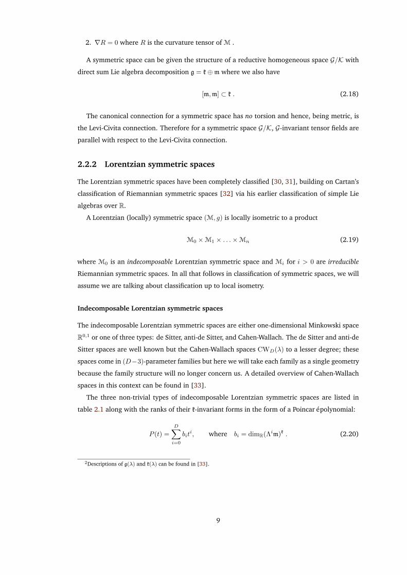
The three non-trivial types of indecomposable Lorentzian symmetric spaces are listed in
table 2.1 along with the ranks of their k-invariant forms in the form of a Poincaré polynomial:
P (t) =
D∑i=0
biti, where bi = dimR(Λim)k . (2.20)
2Descriptions of g(λ) and k(λ) can be found in [33].
9
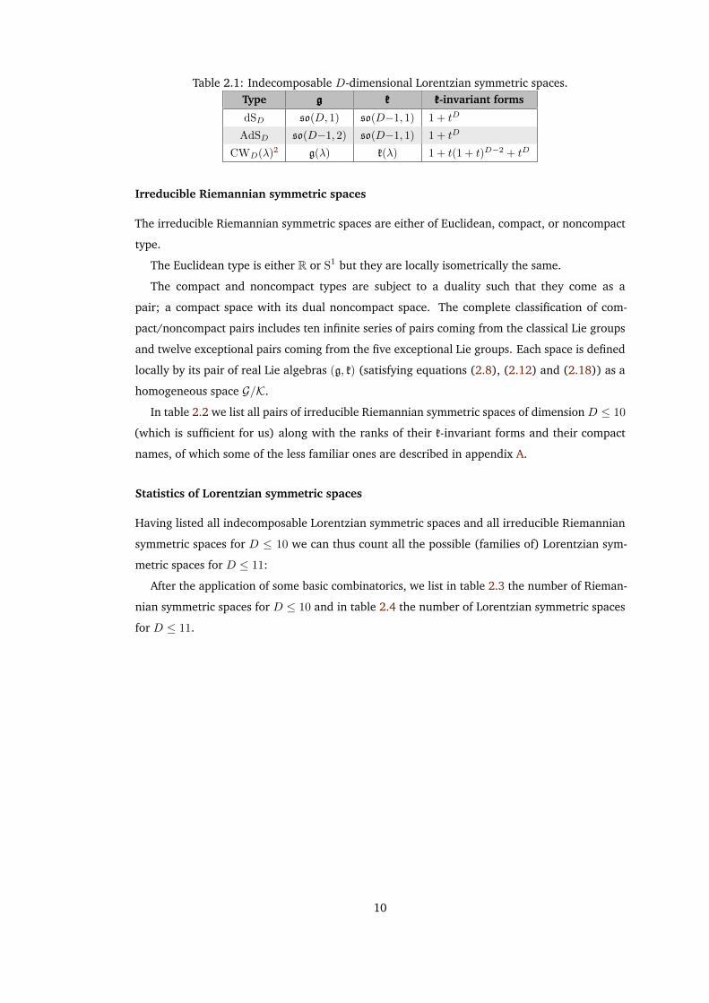
Table 2.1: Indecomposable D-dimensional Lorentzian symmetric spaces.Type ggg kkk kkk-invariant forms
dSD so(D, 1) so(D−1, 1) 1 + tD
AdSD so(D−1, 2) so(D−1, 1) 1 + tD
CWD(λ)2 g(λ) k(λ) 1 + t(1 + t)D−2 + tD
Irreducible Riemannian symmetric spaces
The irreducible Riemannian symmetric spaces are either of Euclidean, compact, or noncompact
type.
The Euclidean type is either R or S1 but they are locally isometrically the same.
The compact and noncompact types are subject to a duality such that they come as a
pair; a compact space with its dual noncompact space. The complete classification of com-
pact/noncompact pairs includes ten infinite series of pairs coming from the classical Lie groups
and twelve exceptional pairs coming from the five exceptional Lie groups. Each space is defined
locally by its pair of real Lie algebras (g, k) (satisfying equations (2.8), (2.12) and (2.18)) as a
homogeneous space G/K.
In table 2.2 we list all pairs of irreducible Riemannian symmetric spaces of dimension D ≤ 10
(which is sufficient for us) along with the ranks of their k-invariant forms and their compact
names, of which some of the less familiar ones are described in appendix A.
Statistics of Lorentzian symmetric spaces
Having listed all indecomposable Lorentzian symmetric spaces and all irreducible Riemannian
symmetric spaces for D ≤ 10 we can thus count all the possible (families of) Lorentzian sym-
metric spaces for D ≤ 11:
After the application of some basic combinatorics, we list in table 2.3 the number of Rieman-
nian symmetric spaces for D ≤ 10 and in table 2.4 the number of Lorentzian symmetric spaces
for D ≤ 11.
10
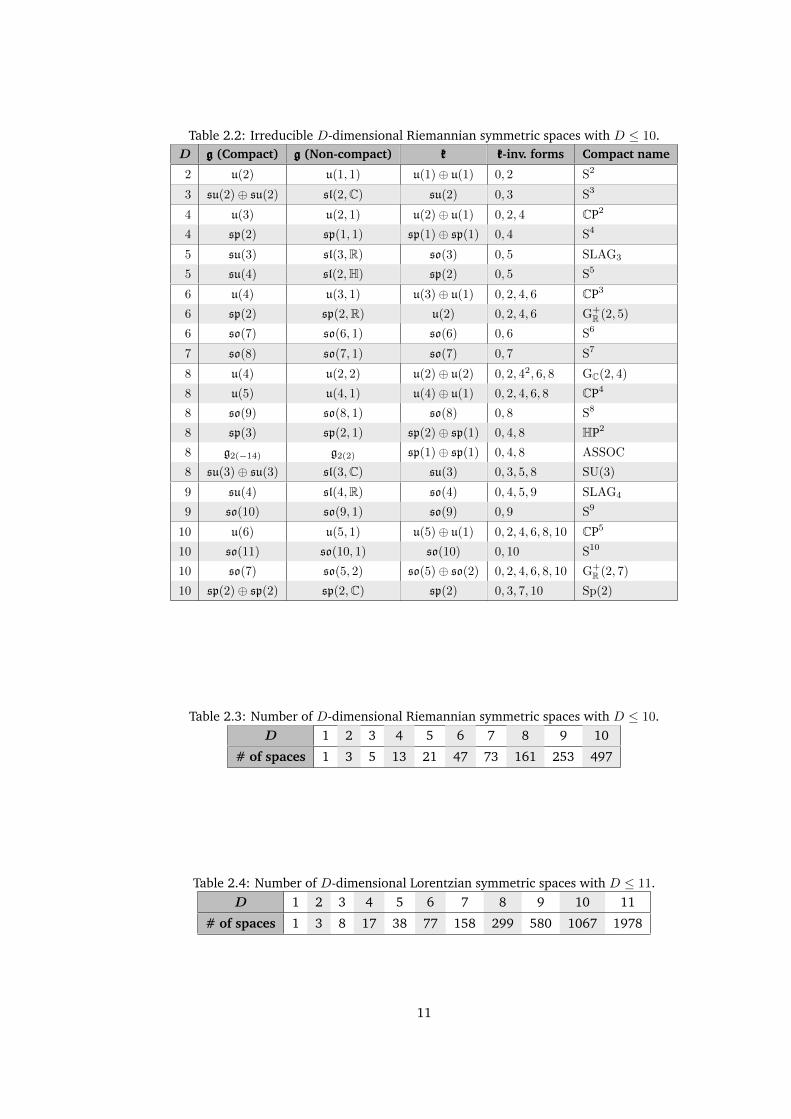
Table 2.2: Irreducible D-dimensional Riemannian symmetric spaces with D ≤ 10.D ggg (Compact) ggg (Non-compact) kkk kkk-inv. forms Compact name
2 u(2) u(1, 1) u(1)⊕ u(1) 0, 2 S2
3 su(2)⊕ su(2) sl(2,C) su(2) 0, 3 S3
4 u(3) u(2, 1) u(2)⊕ u(1) 0, 2, 4 CP2
4 sp(2) sp(1, 1) sp(1)⊕ sp(1) 0, 4 S4
5 su(3) sl(3,R) so(3) 0, 5 SLAG3
5 su(4) sl(2,H) sp(2) 0, 5 S5
6 u(4) u(3, 1) u(3)⊕ u(1) 0, 2, 4, 6 CP3
6 sp(2) sp(2,R) u(2) 0, 2, 4, 6 G+R (2, 5)
6 so(7) so(6, 1) so(6) 0, 6 S6
7 so(8) so(7, 1) so(7) 0, 7 S7
8 u(4) u(2, 2) u(2)⊕ u(2) 0, 2, 42, 6, 8 GC(2, 4)
8 u(5) u(4, 1) u(4)⊕ u(1) 0, 2, 4, 6, 8 CP4
8 so(9) so(8, 1) so(8) 0, 8 S8
8 sp(3) sp(2, 1) sp(2)⊕ sp(1) 0, 4, 8 HP2
8 g2(−14) g2(2) sp(1)⊕ sp(1) 0, 4, 8 ASSOC
8 su(3)⊕ su(3) sl(3,C) su(3) 0, 3, 5, 8 SU(3)
9 su(4) sl(4,R) so(4) 0, 4, 5, 9 SLAG4
9 so(10) so(9, 1) so(9) 0, 9 S9
10 u(6) u(5, 1) u(5)⊕ u(1) 0, 2, 4, 6, 8, 10 CP5
10 so(11) so(10, 1) so(10) 0, 10 S10
10 so(7) so(5, 2) so(5)⊕ so(2) 0, 2, 4, 6, 8, 10 G+R (2, 7)
10 sp(2)⊕ sp(2) sp(2,C) sp(2) 0, 3, 7, 10 Sp(2)
Table 2.3: Number of D-dimensional Riemannian symmetric spaces with D ≤ 10.D 1 2 3 4 5 6 7 8 9 10
# of spaces 1 3 5 13 21 47 73 161 253 497
Table 2.4: Number of D-dimensional Lorentzian symmetric spaces with D ≤ 11.D 1 2 3 4 5 6 7 8 9 10 11
# of spaces 1 3 8 17 38 77 158 299 580 1067 1978
11
Chapter 3
The homogeneity theorem
3.1 Introduction
We motivate and develop the framework for the strong homogeneity theorem for (Poincaré)
supergravity backgrounds. This chapter is based upon work done in collaboration with José
Figueroa-O’Farrill in [1, 2] and builds upon previous work in [34, 35].
Let (M, g,Φ, $) be a supergravity background where (M, g) is an (oriented) connected finite-
dimensional Lorentzian spin manifold with Φ the bosonic field content of the background and $
a real spinor bundle constructed in the usual manner from a (possibly reducible) spin represent-
ation S.
3.2 Killing vectors
Killing vector fields are normally defined with respect to a (pseudo-)Riemannian manifold
because many of their features are contingent on the existence of a metric tensor, but we will
first consider the (tautological) starting case of a smooth manifold so that our extension from
the category of (pseudo-)Riemannian manifolds to that of supergravity backgrounds is more
natural.
We define a Killing vector field on a smooth manifold M to be a vector field K ∈ Γ(TM)
whose flow is a continuous symmetry of the manifold, i.e. Killing vector fields are the infinites-
imal generators of continuous symmetries. In the category of smooth manifolds, we have no
geometrical structure and so Killing vector fields are simply vector fields.
Let a geometrical structure on M be defined by some tensor field A ∈ Γ(TpqM). Then we
define a Killing vector field K to be a vector field whose flow leaves A invariant1, i.e.
LKA = 0 . (3.1)1Perhaps up to gauge transformations.
12
Now, under the Lie bracket of vector fields, for K1,K2 Killing vector fields and tensor field A,
we have
L[K1,K2]A = [LK1,LK2
]A = 0 . (3.2)
Thus the Killing vector fields form a Lie subalgebra of the Lie algebra of vector fields.
Let us turn to the more familiar case of pseudo-Riemannian manifolds whence the geometrical
structure we add is the metric tensor g. A Killing vector field K on a pseudo-Riemannian
manifold (M, g) is a vector field whose flow is isometric, i.e. as in equation (3.1) flowing along
K leaves the metric invariant: LKg = 0 . Rewriting this in terms of the Levi-Civita connection
∇ gives us the Killing equation,
g(∇XK,Y ) + g(X,∇YK) = 0 , (3.3)
where K is a Killing vector field and X,Y any vector field. This means that the canonical
covariant derivative of a Killing vector field on a pseudo-Riemannian manifold is a vector field
skew-symmetric relative to the metric, with the converse also true.
3.2.1 Working at a point
Killing vector fields are uniquely determined [36] at a point m ∈M by their value Km and the
value of their first derivative (∇K)m . In order to parallel transport a Killing vector we must
consider it as the parallel section of a connection on some vector bundle. Concretely, Killing
vector fields are in one-to-one correspondence [37] with sections of the bundle
W := TM⊕ so(TM) , (3.4)
parallel with respect to the (Killing transport)-associated connection,
DX : W → W
(Y,A) 7→ (∇XY +A(X),∇XA−R(X,Y )) ,(3.5)
where A ∈ so(TM), and R ∈ Ω2(so(TM)) is the curvature tensor of (M, g).
We have defined A to be a (metric-relative) skew-symmetric endomorphism of the tangent
bundle and so using equation (3.5) we see that a D-parallel section (K,A) satisfies
0 = −g(A(X), Y )− g(X,A(Y )) = g(∇XK,Y ) + g(X,∇YK) , (3.6)
recovering Killing’s equation equation (3.3).
We may then construct the Lie bracket for D-parallel sections,
[(X,A), (Y,B)] = (A(Y )−B(X), [A,B] +R(X,Y )) . (3.7)
13
We can then see that this is a valid Lie bracket because,
A(Y )−B(X) = −∇YX +∇XY = [X,Y ] , (3.8)
and[A,B] +R(X,Y ) = −R(·, X)Y +A(B) +R(·, Y )X −B(A)
= −(∇A)Y −A(∇Y ) + (∇B)X +B(∇X)
= −∇ (A(Y )−B(X))
= −∇[X,Y ] ,
(3.9)
and so
[(X,A), (Y,B)] = ([X,Y ],−∇[X,Y ]) , (3.10)
which is the expected extension of the standard Lie bracket on vector fields. We note that this Lie
bracket fails to satisfy the Jacobi identity if extended to sections of W that are not D-parallel.
Thus if we wish to work with Killing vectors at a point m ∈M, we can consider Killing vector
fields as D-parallel sections of W, with parallel transport on M by D.
3.2.2 Supergravity Killing vectors
Now, to further specialise, we are interested in Killing vector fields of a supergravity background
(M, g,Φ, $) and here we may now consider the collection of bosonic fields Φ to be an additional
geometric structure. Hence and again, for the flow of K to be a continuous symmetry of the
manifold, now in addition to being an isometry it must also leave Φ invariant: LKΦ = 0.
If we have gauge fields, then it is their field strengths that we will consider as the relevant
objects in Φ and we require invariance only up to gauge transformations. This will always be
the implication when claiming LKΦ = 0.
We thus define the Lie algebra of Killing vector fields of a supergravity background:
g0 := (K,−∇K) ∈ Γ(W) : DX(K,−∇K) = 0 = LKΦ, ∀ X ∈ Γ(TM) . (3.11)
3.3 Killing spinors
The action of a supergravity theory is invariant under local supersymmetry transformations
comprised of the field content of the theory and parametrised by arbitrary sections of the spinor
bundle we call the supersymmetry parameter. For a classical supergravity background, which
is a solution to the supergravity field equations in which all fermionic fields are set to zero, the
supersymmetry transformations of the bosonic fields all disappear automatically and so we are
left with the transformations of the fermionic fields which depend upon Φ and the spinorial
supersymmetry parameter ε. These transformations must disappear for the background to have
14
any residual local supersymmetry and this means the existence of Killing spinor fields ε that
render the transformations trivial.
Thus, the Killing spinor equations are the system of equations originating from requiring the
disappearance of the supersymmetry transformations of the fermionic content of the theory.
The supersymmetry transformation of a gravitino yields a connection D = ∇ + Ω on $ (with
Ω ∈ T∗M ⊗ End($) depending upon Φ). The supersymmetry transformation of a dilatino or
gaugino yields an (algebraic) bundle map on $ we will denote by P or Q respectively. Of course,
not all theories have dilatinos or gauginos but we always have at least a gravitino and so a
connection D. Note that D is not necessarily a metric connection and is not in general induced
from a connection on the tangent bundle; it is a true spinor connection.
Note that Φ is a collection of bosonic fields all living in the exterior algebra bundle and
their action on the spinor bundle is via the globalisation of the exterior algebra vector space
isomorphism with the Clifford algebra (see appendix B.5), of which the spinor bundle is a bundle
of modules.
The connection D, P, and Q are all linear bundle maps on $ depending upon Φ and the
intersection of their kernels,
K := kerD ∩ kerP ∩ kerQ ⊂ $ (3.12)
forms the vector subbundle of Killing spinor fields so we define the vector space of Killing spinor
fields to be
g1 := Γ(K) = ε ∈ Γ($) : Dε = Pε = Qε = 0 . (3.13)
3.3.1 Working at a point
If we wish to work with Killing spinors at a point m ∈M, we note that D,P, and Q all contain
at most first order derivatives and so a Killing spinor field is uniquely determined by its value at
a point, with parallel transport on M by D.
3.3.2 Supersymmetry
The number of supersymmetries of a background is the dimension of the odd subspace of the
supersymmetry superalgebra of the background. We define ν to be the fraction of supersymmetry
preserved with respect to the maximum supersymmetry of the theory.
It is clear that the number of supersymmetries of a background is also encoded in the rank
of the subbundle of Killing spinor fields of a background. Indeed,
ν =rankK
rank $. (3.14)
15
3.4 The Killing superalgebra
3.4.1 Lie superalgebras
A superalgebra A is a Z2-graded K-algebra, i.e. a K-algebra A that decomposes into two
subspaces A = A0 ⊕A1 where the product operator respects the grading Ai ×Aj → Ai+j .
A Lie superalgebra [38] g = g0 ⊕ g1 is a superalgebra whose product operator is the super-
commutator [·,·] that additionally satisfies, for x, y, z ∈ g:
• Super skew-symmetry:
[x, y] = −(−1)|x||y|[y, x] (3.15)
• Super Jacobi identity:
(−1)|x||z|[x, [y, z]] + (−1)|y||x|[y, [z, x]] + (−1)|z||y|[z, [x, y]] = 0 (3.16)
Thus g0 is a Lie algebra and g1 is a g0-module.
3.4.2 The symmetry superalgebra
We may construct a Lie superalgebra g = g0 ⊕ g1 where g0 is the Lie algebra of (Φ-preserving)
Killing vector fields (equation (3.11)) and g1 is the vector space of Killing spinor fields (equa-
tion (3.13)). We will call this the symmetry superalgebra of a background and in order to show
that this may form a Lie superalgebra we first define the supercommutator for each grade
combination:
[·,·] : g0 ⊗ g0 → g0
We have already seen that g0 is a Lie subalgebra of Killing vector fields with respect to Lie bracket
defined in equation (3.7) and so we define the even-even bracket to be
[·,·] : g0 ⊗ g0 → g0
((X,A), (Y,B)) 7→ (A(Y )−B(X), [A,B] +R(X,Y )) .(3.17)
[·,·] : g0 ⊗ g1 → g1
We define the even-odd bracket using the spinorial Lie derivative [39] (see appendix B.10):
[·,·] : g0 ⊗ g1 → g1
((K,−∇K), ε) 7→ LKε = ∇Kε+ 14κ1(∇K) · ε ,
(3.18)
where, as defined in appendix B.4.3, κ1 is the sign convention used to define the gamma matrix
representation of the Clifford algebra with ΓaΓb + ΓbΓa = 2κ1ηab1.
16
Now, for a Killing vector field K and any spinor field ε and vector field X, a standard identity
of the spinorial Lie derivative is
LK∇Xε = ∇XLKε+∇[K,X]ε . (3.19)
By construction we have LKΦ = 0 and so LKΩ(Φ) = 0; as such this identity extends to D,
yielding
DXLKε = LKDXε−D[K,X]ε , (3.20)
and so for D-parallel ε this tells us that LKε is also D-parallel. Also, since P and Q are linear
bundle maps depending only on Φ we have
[LK ,P] = [LK ,Q] = 0 . (3.21)
Thus ε Killing implies that LKε is also Killing. As such the even-odd bracket is well-defined
when we impose its skew-symmetry.
[·,·] : g1 ⊗ g1 → g0
The brackets so far have been defined in full generality and do not depend on the particulars of
the supergravity theory or its spinor bundle $. However, the odd-odd bracket will be different.
Viewing the real spinor bundle as a bundle of Clifford modules, let us presume that we have
a (real) pin-invariant spinor inner product J·,·K : S × S → R that naturally globalises with an
abuse of notation to J·,·K : $× $→ R. The details of this inner product will depend upon the
signature of the Clifford algebra and the spin representation S of the spinor bundle but because
we are working with a real spinor bundle will either be real symmetric or real symplectic.
Let us denote the Lorentzian inner product on TM as L·,·M. Then we define the squaring
map Ξ : $× $→ TM as the transpose of the Clifford action relative to this spinor inner product
and the Lorentzian inner product, i.e. for all ε1,2 ∈ Γ($), X ∈ Γ(TM),
LΞ(ε1, ε2), XM = Jε1, X[ · ε2K . (3.22)
We will require that the bilinear Jε1, X[ · ε2K be symmetric in ε1,2 and so, looking ahead, also
the squaring map. Thus, denoting the adjoint of X[ with respect to the spinor inner product by
X[ and the symmetry of the spinor inner product by κ3 we have
Jε1, X[ · ε2K = JX[ · ε1, ε2K = κ3Jε2, X
[ · ε1K!= Jε2, X
[ · ε1K , (3.23)
and so in order for the bilinear to be symmetric, we require complementarity of the inner
product’s symmetry and its 1-form adjoint, i.e. X[ = κ3X[ . Given this 1-form only carries
manifold indices, this means that its adjoint in the Clifford bundle must be its adjoint with
17
respect to a pinor inner product. The adjoint of a rank-one element of the Clifford algebra with
respect to a pinor inner product depends upon which involution induced the inner product. It
is self-adjoint under the check involution and anti-self-adjoint under the hat involution. Thus
we require either an R-symplectic pinor inner product induced from the hat involution or an
R-symmetric pinor inner product induced from the check involution. We note that such a pinor
inner product always exists in Lorentzian signature with d ≤ 11 .
Now, Ω(X) acts on spinors via the Clifford action and so the most general form in which we
can construct a covariant Ω(X) is:
Ω(X) =∑i
aiW(ni)
i ·X[ + biX
[ ·W (ni)
i , (3.24)
where W (ni)
i is some Z-valued ni-form constructed from objects in Φ with $ a bundle of Z-
modules, and ai, bi are real constants. We will assume that we only have a single term because
our argument will distribute over the sum, and so we take
Ω(X) = aW (n) ·X[ + bX[ ·W (n) . (3.25)
The adjoint relative the spinor inner product is then
Ω(X) = κ3
(bW (n) ·X[ + aX[ · W (n)
). (3.26)
Now, for ε1,2 Killing spinors and X,Y ∈ Γ(TM), using equation (3.22) we have
L∇XΞ(ε1, ε2), Y M = XLΞ(ε1, ε2), Y M− LΞ(ε1, ε2),∇XY M
= XJε1, Y[ · ε2K− Jε1, (∇XY [) · ε2K
= J∇Xε1, Y[ · ε2K + Jε1, Y
[ · ∇Xε2K
= −JΩ(X) · ε1, Y[ · ε2K− Jε1, Y
[ · Ω(X) · ε2K
= −Jε1, Ω(X) · Y [ · ε2K− Jε1, Y[ · Ω(X) · ε2K
= −Jε1,κ3
(bW (n) ·X[ + aX[ · W (n)
)· Y [ · ε2K
−Jε1, Y[ ·(aW (n) ·X[ + bX[ ·W (n)
)· ε2K
= −bJε1,(Y [ ·X[ ·W (n) + κ3W
(n) ·X[ · Y [)· ε2K
−aJε1,(Y [ ·W (n) ·X[ + κ3X
[ · W (n) · Y [)· ε2K .
(3.27)
Equation (3.3) tells us that in order for Ξ(ε1, ε2) to be a Killing vector field, L∇XΞ(ε1, ε2), Y M
must be skew-symmetric in X,Y . This is clearly satisfied if (although not iff) for each term in
Ω(X),
W (n) = −κ3W(n) . (3.28)
In order for Ξ(ε1, ε2) to be a supergravity Killing vector field, it must also leave Φ invariant
18
and to show this will often require us to invoke the field equations of the particular theory.
We will construct the spinor inner product case by case for each supergravity theory and show
that it satisfies, for κ3 the symmetry of the pinor inner product:
1. X[ = κ3X[ , and
2. W (n) = −κ3W(n) , and
3. LΞ(ε1,ε2)Φ = 0 .
Let us assume its existence for the rest of this chapter. We can then extend the squaring map
naturally (and also call this the squaring map) to
χ : $⊗ $ → W
(ε1, ε2) 7→ (Ξ(ε1, ε2),−∇Ξ(ε1, ε2)) ,(3.29)
whose restriction to the subbundle of Killing spinors we will use to define the odd-odd bracket:
[·,·] : g1 ⊗ g1 → g0
(ε1, ε2) 7→ χ(ε1, ε2) ,(3.30)
3.4.2.1 Super Jacobi identity
[g0, g0, g0]
This component of the super Jacobi identity is nothing more than the standard Jacobi identity
of g0 as a Lie algebra. We have shown in section 3.2.1 that the Lie bracket of equation (3.7)
is equivalent to the standard Lie bracket, whence its Jacobi identity follows from the Jacobi
identity of the Lie algebra of vector fields with the standard Lie bracket.
[g0, g0, g1]
This identity is, for X,Y, ε Killing,
[X, [Y, ε]] + [Y, [ε,X]] + [ε, [X,Y ]]!= 0 . (3.31)
Now, the spinorial Lie derivative satisfies
L[X,Y ]ε = LXLY ε− LY LXε, (3.32)
which is precisely this component of the super Jacobi identity.
19
[g0, g1, g1]
This identity is, for K, ε1,2 Killing,
[K, [ε1, ε2]]!= [ε1, [K, ε2]] + [[K, ε1], ε2] . (3.33)
This is equivalent to requiring that, with X any vector field,
LLKΞ(ε1, ε2), XM != JLKε1, X
[ · ε2K + Jε,X[ · LKε2K . (3.34)
The left hand side is
LLKΞ(ε1, ε2), XM = L∇KΞ(ε1, ε2)−∇Ξ(ε1,ε2)K,XM
= J∇Kε1, X[ · ε2K + Jε1, X
[ · ∇Kε2K− L∇KΞ(ε1, ε2), XM
= J∇Kε1, X[ · ε2K + Jε1, X
[ · ∇Kε2K + Jε1, (∇XK[) · ε2K .
(3.35)
The right hand side is
JLKε1, X[ · ε2K + Jε1, X
[ · LKε2K = J∇Kε1, X[ · ε2K + Jε1, X
[ · ∇Kε1K
− 14κ1Jε1,
((∇K) ·X[ −X[ · (∇K)
)· ε2K
= J∇Kε1, X[ · ε2K + Jε1, X
[ · ∇Kε1K
− 14κ1Jε1,−4κ1(∇XK[) · ε2K
= J∇Kε1, X[ · ε2K + Jε1, X
[ · ∇Kε2K + Jε1, (∇XK[) · ε2K ,(3.36)
where we have used the fact that∇K is anti-self-adjoint with respect to the spinor inner product
(which is true for any pin-invariant spinor inner product).
Thus, this component of the super Jacobi identity is satisfied.
[g1, g1, g1]
This identity is, for ε1,2,3 Killing,
[ε1, [ε2, ε3]] + [ε3, [ε1, ε2]] + [ε2, [ε3, ε1]]!= 0 . (3.37)
We note that the odd-odd bracket, being symmetric and bilinear, is determined by its value
on the diagonal via the polarisation identity:
2[ε1, ε2] = [ε1 + ε2, ε1 + ε2]− [ε1, ε1]− [ε2, ε2] , (3.38)
20
and thus equation (3.37) is exactly equivalent to, for ε Killing,
[ε, [ε, ε]]!= 0 . (3.39)
As with the construction of the odd-odd bracket, we will generally have to appeal to the
details of the particular supergravity theory to show that this identity holds.
3.4.3 The Killing superalgebra
We have elucidated the construction of the symmetry superalgebra of a supergravity background.
However, we are particularly interested in the canonical ideal of this superalgebra that we will
call the Killing superalgebra:
g := span([g1, g1])⊕ g1 ⊂ g . (3.40)
This is the sub-superalgebra of the symmetry superalgebra, constructed entirely from the Killing
spinors of a background.
3.5 The theorem
3.5.1 Motivation
We have seen that, given we are able to construct a suitable squaring map, Killing spinor fields
of a supergravity background square to Killing vector fields of the background and indeed, given
a vector space of Killing spinor fields g1, we may construct a Lie algebra of Killing vector fields
[g1, g1]. This fact does not even require the structure of a Lie superalgebra — given we have
the squaring map, we see that all super Jacobi identity brackets are satisfied automatically
apart from the [g1, g1, g1] component. For what follows, it will be immaterial to us whether this
component of the identity is satisfied. We will call such a structure an almost Killing superalgebra,
i.e. we have the structure of a Killing superalgebra as described in section 3.4 except that the
[g1, g1, g1] component of the super Jacobi identity is not necessarily satisfied.
Now, supposing we have an almost Killing superalgebra on a supergravity background, we see
that supersymmetries of the background generate conventional symmetries of the background.
The more conventional symmetries that a background has, the more geometrically simple it is,
and there are a number of refinements for describing geometrical simplicity that we may call
upon. So a natural question to ask is if there are any thresholds of supersymmetry that saturate
the requirements for a particular refinement of geometrical simplicity.
This line of reasoning led to Patrick Meessen’s homogeneity conjecture, reviewed in [34]:
All supergravity backgrounds with ν > 12 are homogeneous.
This is of course the most natural refinement of geometrical simplicity to aim for — homo-
geneity of a background essentially means that the symmetries of the background saturate the
21
tangent bundle, or in other words the symmetries make any point in the background look much
like any other point in the background, because we can transitively flow along symmetries.
We must however modify this slightly, because in supergravity we only work with local
metrics and the background may not in general be complete. As such, the more relevant concept
is local homogeneity (see section 2.1.5) and so the conjecture becomes
All supergravity backgrounds with ν > 12 are locally homogeneous.
We note that there are, of course, no counterexamples to this conjecture, and as we will see,
nor can there be.
3.5.2 Working at a point
We have shown that both Killing spinor fields and Killing vector fields, given as sections of the
appropriate vector bundles parallel with respect to the appropriate connections, may be defined
entirely by their value at a point, with parallel transport around M via said connections. As such,
let us now permanently fix a point m ∈M:
The tangent bundle TM may be obtained as the vector bundle associated to the spin bundle
through the vector representation V of the correspondent special orthogonal group. As such, we
identify the tangent bundle fiber TmM with V.
The spinor bundle $ is the vector bundle associated to the spin bundle through the real (not
necessarily irreducible) spinor representation S. As such, we identify the spinor bundle fiber $m
with S.
The spinor bundle subbundle of Killing spinors then restricts at a point to a subspace of S,
W := Km ⊂ S , (3.41)
and the squaring map restricts at a point to the map,
ϕ := Ξm : S × S → V . (3.42)
3.5.3 Proof
We aim to show that if dimW > 12 dimS (i.e. ν > 1
2), then the restriction of Ξm to W is
surjective, i.e.
ϕ∣∣W :W ×W V . (3.43)
This would mean that V and so TmM are spanned by the values of supergravity Killing vec-
tors at m and so we can flow along supergravity Killing vector fields to any point in a local
neighbourhood U around m. Thus the background is locally homogeneous.
Before continuing however, we will need to impose one more (not unreasonable) requirement
on the squaring map: that squaring a single Killing spinor produces a Killing vector that is causal,
22

i.e null or timelike with respect to the Lorentzian inner product:
κ0|Ξ(ε, ε)|2 = κ0LΞ(ε, ε),Ξ(ε, ε)M = κ0Jε,Ξ(ε, ε)[ · εK ≤ 0 , (3.44)
where, as defined in appendix C, κ0 is the sign convention of the metric with κ0 = +1 denoting
a mostly plus metric and κ0 = −1 a mostly minus metric.
This requirement will be necessary for our proof and we will have to show this for each
supergravity theory.
Let dimW > 12 dimS.
Now, we have the Lorentzian inner product on V and so as V is thus a semi-inner product
space, for any subspace U ⊂ V we have dimU + dimU⊥ = dimV where the perpendicular
complement is defined as
U⊥ = x ∈ V : Lx, uM = 0 ∀ u ∈ U . (3.45)
Thus, on dimensional grounds, the map ϕ∣∣W is surjective iff the perpendicular complement
of its image (relative to the Lorentzian inner product on V) is trivial,
0 != (Imϕ
∣∣W)⊥ = x ∈ V : Lx, kM = 0 ∀ k ∈ Imϕ
∣∣W . (3.46)
Using the definition of the squaring map in equation (3.22) this is true iff the only vector
x ∈ V satisfying
Jw1, x[ · w2K = 0 , (3.47)
for all w1,2 ∈ W is the zero vector x = 0.
Now, let us assume that a vector x 6= 0 exists that satisfies equation (3.47).
The spinor inner product on S also makes S a semi-inner product space, and so forW ⊂ S
we have dimW + dimW⊥ = dimS where the perpendicular complement is defined as
W⊥ = ε ∈ S : Jε, wK = 0 ∀ w ∈ W . (3.48)
It is clear that such an x is thus necessarily a map
x :W →W⊥ . (3.49)
Now, dimW + dimW⊥ = dimS but dimW > 12 dimS, and so dimW⊥ < dimW. Thus,
simply on dimensional grounds, as a map x must have non-trivial kernel. Yet the action of x on
W is the Clifford action and so
x2 = κ1Lx, xM1 , (3.50)
whence x has non-trivial kernel iff it is null, Lx, xM != 0.
23
Thus, backtracking to equation (3.46), the space (Imϕ∣∣W)⊥ must be spanned by null vectors
in V and so is a totally null subspace of V. Any null subspace of a Lorentzian vector space is
at most 1-dimensional (see appendix D) and so dim(Imϕ∣∣W)⊥ ≤ 1. If dim(Imϕ
∣∣W)⊥ = 0 then
(Imϕ∣∣W)⊥ is of course trivial and so ϕ
∣∣W is surjective as desired. Let us then assume the case
dim(Imϕ∣∣W)⊥ = 1 whence (Imϕ
∣∣W)⊥ is spanned by the null vector x.
The perpendicular complement of a null subspace of a Lorentzian vector space contains only
itself and spacelike vectors (see appendix D) and so Imϕ∣∣W is spanned by x and spacelike vectors.
However, we earlier imposed that the squaring map acting on a single Killing spinor must only
produce causal Killing vectors whence they are not spacelike and so they are necessarily collinear
with x. Thus
ϕ(ε, ε) = λ(ε)x (3.51)
for some function λ :W → R.
Now, we consider the squaring map on two different Killing spinors, ϕ(ε1, ε2) for ε1,2 ∈ W.
By polarisation we have
2ϕ(ε1, ε2) = ϕ(ε1 + ε2, ε1 + ε2)− ϕ(ε1, ε1)− ϕ(ε2, ε2)
= λ(ε1 + ε2)x− λ(ε1)x− λ(ε2)x
= (λ(ε1 + ε2)− λ(ε1)− λ(ε2))x ,
(3.52)
whence Imϕ∣∣W is collinear with x and so dim Imϕ
∣∣W = 1.
But we already know that dim(Imϕ∣∣W)⊥ = 1 and so dimV = dim Imϕ
∣∣W+dim(Imϕ
∣∣W)⊥ =
2. For dimV = D > 2 we thus have a contradiction and so dim(Imϕ∣∣W)⊥ = 0 whence ϕ
∣∣W
surjects onto V and we have shown local homogeneity of the background.
3.5.4 Summary
Let us recap by summarising the necessary requirements for the homogeneity theorem to apply.
We must have a supergravity background (M, g,Φ, $, J·,·K) where (M, g) is a connected
(D > 2)-dimensional Lorentzian spin manifold, Φ the bosonic field content of the background,
$ a real spinor bundle constructed in the usual manner from a (possibly reducible) spinor
representation S, and J·,·K a pin-invariant spinor inner product with symmetry κ3 on $. We
construct the squaring map Ξ : $× $→ TM using equation (3.22). Then we require:
1. For X ∈ Γ(TM), the squaring map must be symmetric and so we require:
X[ = κ3X[ , and (3.53)
2. For ε1,2 ∈ Γ(K) two Killing spinor fields, the vector field K = Ξ(ε1, ε2) produced by the
squaring map must be a Killing vector field and so we require that LKg = 0. Thus, for Ω
24
taking the form described in equation (3.24), it is sufficient that all W (n) satisfy:
W (n) = −κ3W(n) , and (3.54)
3. For ε ∈ Γ(K) a single Killing spinor field, the Killing vector field K = Ξ(ε, ε) produced by
the squaring map must be causal and so we require:
κ0LK,KM ≤ 0 , and (3.55)
4. For ε1,2 ∈ Γ(K) two Killing spinor fields, the Killing vector field K = Ξ(ε1, ε2) produced
by the squaring map must be a supergravity Killing vector field and so we require:
LKΦ = 0 . (3.56)
Satisfying equations (3.53), (3.54) and (3.56) will give us an almost Killing superalgebra and
then also satisfying equation (3.55) allows us to deduce local homogeneity of the background
using the almost Killing superalgebra. Note that equations (3.53) to (3.55) are all constructed
using only the connection D but showing that equation (3.56) is satisfied will in general require
the invocation of P and Q.
If we wish to construct a full Killing superalgebra we must additionally show that the
[g1, g1, g1] component of the super Jacobi identity is satisfied as described in section 3.4.2.1
which means requiring that for ε ∈ Γ(K) a single Killing spinor field, the Killing vector field
K = Ξ(ε, ε) produced by the squaring map must leave it invariant:
LKε = 0 . (3.57)
25
Chapter 4
Application of the theorem
4.1 Introduction
Using the results from chapter 3, we run through the application of the strong homogeneity
theorem to a number of top-dimensional Poincaré supergravities. In some cases (sections 4.2.7
and 4.3.6), we refer to the original literature for particular results necessary to demonstrate the
existence of the Killing superalgebra. This chapter is based upon work done in collaboration
with José Figueroa-O’Farrill in [1, 2]
4.2 D = 11
4.2.1 Introduction
The Killing superalgebra of D = 11 supergravity was described in [35] and the homogeneity
theorem in [1]. We briefly review these constructions in our formalism. The homogeneity
theorem for D = 11 supergravity places a new and firm control on highly supersymmetric
D = 11 supergravity backgrounds.
4.2.2 Conventions
In the original construction of D = 11 supergravity [19], the sign conventions adopted are
(κ0,κ1) = (−1,+1). Other authors use conventions (−1,−1) [35] and (+1,+1) [40]. Conven-
tions with κ0 = κ1 have a C`(1, 10)-module spinor representation and spinors are real Majorana
whereas for κ0 = −κ1 the spinor representation is a C`(10, 1)-module and they are imaginary
pseudo-Majorana. We will follow [35] and adopt the conventions (κ0,κ1) = (−1,−1).
4.2.3 Definition
The field content of D = 11 supergravity (with all fields transforming in varying representations
of SO(9)) is:
26
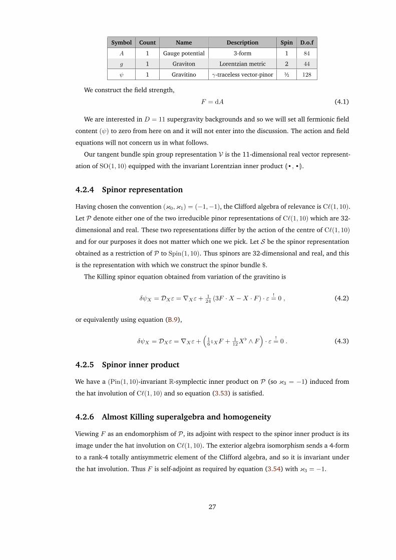
Symbol Count Name Description Spin D.o.f
A 1 Gauge potential 3-form 1 84
g 1 Graviton Lorentzian metric 2 44
ψ 1 Gravitino γ-traceless vector-pinor 3⁄2 128
We construct the field strength,
F = dA (4.1)
We are interested in D = 11 supergravity backgrounds and so we will set all fermionic field
content (ψ) to zero from here on and it will not enter into the discussion. The action and field
equations will not concern us in what follows.
Our tangent bundle spin group representation V is the 11-dimensional real vector represent-
ation of SO(1, 10) equipped with the invariant Lorentzian inner product L·,·M.4.2.4 Spinor representation
Having chosen the convention (κ0,κ1) = (−1,−1), the Clifford algebra of relevance is C`(1, 10).
Let P denote either one of the two irreducible pinor representations of C`(1, 10) which are 32-
dimensional and real. These two representations differ by the action of the centre of C`(1, 10)
and for our purposes it does not matter which one we pick. Let S be the spinor representation
obtained as a restriction of P to Spin(1, 10). Thus spinors are 32-dimensional and real, and this
is the representation with which we construct the spinor bundle $.
The Killing spinor equation obtained from variation of the gravitino is
δψX = DXε = ∇Xε+ 124 (3F ·X −X · F ) · ε !
= 0 , (4.2)
or equivalently using equation (B.9),
δψX = DXε = ∇Xε+(
16 ιXF + 1
12X[ ∧ F
)· ε !
= 0 . (4.3)
4.2.5 Spinor inner product
We have a (Pin(1, 10)-invariant R-symplectic inner product on P (so κ3 = −1) induced from
the hat involution of C`(1, 10) and so equation (3.53) is satisfied.
4.2.6 Almost Killing superalgebra and homogeneity
Viewing F as an endomorphism of P, its adjoint with respect to the spinor inner product is its
image under the hat involution on C`(1, 10). The exterior algebra isomorphism sends a 4-form
to a rank-4 totally antisymmetric element of the Clifford algebra, and so it is invariant under
the hat involution. Thus F is self-adjoint as required by equation (3.54) with κ3 = −1.
27
We construct the squaring map as described in equation (3.22) and, choosing a pseudo-
orthonormal basis e
µ for V and corresponding gamma matrices (see appendix B.11.1) for P, the
squaring map takes the concrete form,
Ξ(ε1, ε2) = Jε1,Γµε2K e
µ = ε1Γµε2
e
µ = ε†1Γ0Γµε2
e
µ , (4.4)
where we denote the Dirac adjoint ε := ε†Γ0 .
Now, if we look at the e
0 component of a vector K = Ξ(ε, ε) obtained from the squaring map,
we see that for non-zero ε,
K0 = ε†Γ0Γ0ε = −ε†ε = −ε†ε = −|ε|2 < 0 , (4.5)
This means that a vector field K constructed by squaring a single non-zero spinor field ε is
necessarily causal because otherwise we could of course Lorentz-transform to the rest frame
where K0 = 0. Thus equation (3.55) is satisfied.
Using equation (4.2) we have for a Killing spinor ε,
∇Xε = −Ω(X) · ε = −(
16 ιXF + 1
12X[ ∧ F
)· ε . (4.6)
The adjoint of Ω(X) with respect to the spinor inner product is its image under the hat involution,
Ω(X) = 16 ιXF −
112X
[ ∧ F . (4.7)
Let us define a 2-form θ constructed from two Killing spinor fields ε1,2 via the spinor inner
product as
θµν = Jε1,Γµνε2K . (4.8)
Then we have∇µθνρ = ∇µJε1,Γνρε2K
= J∇µε1,Γνρε2K + Jε1,Γνρ∇µε2K
= −JΩµε1,Γνρε2K− Jε1,ΓνρΩµε2K
= −Jε1,(
ΓνρΩµ + ΩµΓνρ
)ε2K .
(4.9)
Now, we have (with liberal use of equation (B.13))
ΓνρΩµ + ΩµΓνρ = 112·4!Fστκλ
(ΓνρΓ
στκλµ − ΓστκλµΓνρ
)+ 2
3·4!Fτκλ
µ
(ΓνρΓ
τκλ + ΓτκλΓνρ)
= 20 · 112·4!Fστκλgαµδ
[α[ν Γ
στκλ]ρ] + 2 · 2
3·4!Fµτκλ
(Γ τκλνρ − 6δ
[τκ[νρ]Γ
λ])
= 83·4!Fστκ[νΓ στκ
ρ]µ + 23·4!Fστκλgµ[νΓ στκλ
ρ] + 43·4!Fµτκλ Γ τκλ
νρ − 84!Fµνρλ Γλ
=(
83·4!Fστκ[νΓ στκ
ρ]µ − 43·4!Fστκµ Γ στκ
νρ
)+ 2
3·4!Fστκλgµ[νΓ στκλρ] − 8
4!Fµνρλ Γλ
(4.10)
If we antisymmetrise this expression over (µ, ν, ρ), the first and second terms disappear and we
28
are left with
(dθ)µνρ = ∇[µθνρ] = 13!FµνρλJε1,Γ
λε2K . (4.11)
Thus for a Killing vector field produced from two Killing spinors ε1,2 via the squaring map
K = Ξ(ε1, ε2), we have
dθ = ιKF , (4.12)
and as such, dιKF = 0, and since F is closed we then have
LKF = ιKdF + dιKF = 0 , (4.13)
whence K preserves F and equation (3.56) is satisfied.
We have thus satisfied all the sufficient requirements to have an almost Killing superalgebra
and for the homogeneity theorem to apply.
4.2.7 Killing superalgebra
The satisfaction of equation (3.57) (the [g1, g1, g1] super Jacobi identity) is shown in detail in
[35] and demonstrates that there is a Killing superalgebra for D = 11 supergravity.
4.3 D = 10 type IIB
4.3.1 Introduction
The Killing superalgebra ofD = 10 type IIB supergravity was described in [41] and the homogen-
eity theorem in [1]. We briefly review these constructions in our formalism. The homogeneity
theorem for D = 11 supergravity places a new and firm control on highly supersymmetric
D = 10 type IIB supergravity backgrounds.
4.3.2 Conventions
In the constructing literature of D = 10 Type IIB supergravity [42, 43, 44], the sign conventions
adopted are (κ0,κ1) = (−1,+1). Other authors use the convention (+1,+1) [45, 41]. Conven-
tions with κ0 = κ1 have a C`(1, 9)-module spinor representation whereas for κ0 = −κ1 the
spinor representation is a C`(9, 1)-module. Both have real Majorana-Weyl spinors and we will
adopt the conventions (κ0,κ1) = (−1,−1).
4.3.3 Definition
The field content of type IIB supergravity (with all fields transforming in varying representations
of SO(8)) is:
29
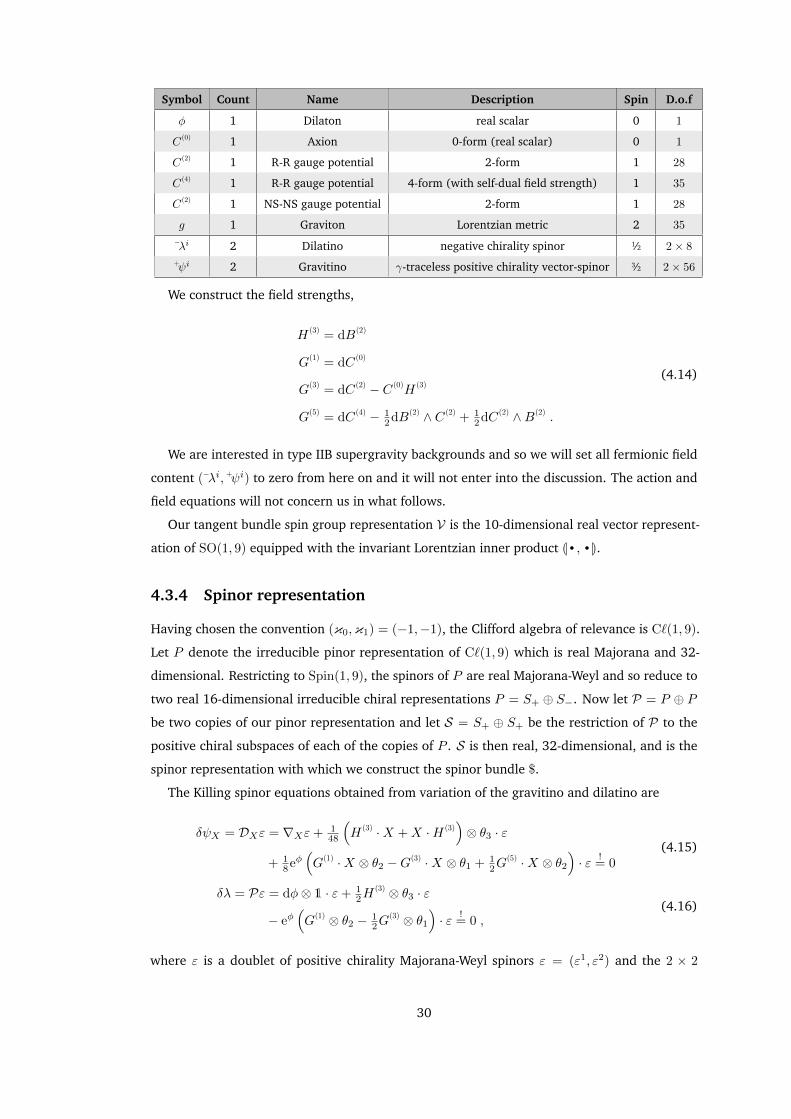
Symbol Count Name Description Spin D.o.f
φ 1 Dilaton real scalar 0 1
C (0) 1 Axion 0-form (real scalar) 0 1
C (2) 1 R-R gauge potential 2-form 1 28
C (4) 1 R-R gauge potential 4-form (with self-dual field strength) 1 35
C (2) 1 NS-NS gauge potential 2-form 1 28
g 1 Graviton Lorentzian metric 2 35
−λi 2 Dilatino negative chirality spinor 1⁄2 2× 8
+ψi 2 Gravitino γ-traceless positive chirality vector-spinor 3⁄2 2× 56
We construct the field strengths,
H (3) = dB(2)
G(1) = dC (0)
G(3) = dC (2) − C (0)H (3)
G(5) = dC (4) − 12dB(2) ∧ C (2) + 1
2dC (2) ∧B(2) .
(4.14)
We are interested in type IIB supergravity backgrounds and so we will set all fermionic field
content (−λi, +ψi) to zero from here on and it will not enter into the discussion. The action and
field equations will not concern us in what follows.
Our tangent bundle spin group representation V is the 10-dimensional real vector represent-
ation of SO(1, 9) equipped with the invariant Lorentzian inner product L·,·M.4.3.4 Spinor representation
Having chosen the convention (κ0,κ1) = (−1,−1), the Clifford algebra of relevance is C`(1, 9).
Let P denote the irreducible pinor representation of C`(1, 9) which is real Majorana and 32-
dimensional. Restricting to Spin(1, 9), the spinors of P are real Majorana-Weyl and so reduce to
two real 16-dimensional irreducible chiral representations P = S+ ⊕ S−. Now let P = P ⊕ P
be two copies of our pinor representation and let S = S+ ⊕ S+ be the restriction of P to the
positive chiral subspaces of each of the copies of P . S is then real, 32-dimensional, and is the
spinor representation with which we construct the spinor bundle $.
The Killing spinor equations obtained from variation of the gravitino and dilatino are
δψX = DXε = ∇Xε+ 148
(H (3) ·X +X ·H (3)
)⊗ θ3 · ε
+ 18eφ
(G(1) ·X ⊗ θ2 −G(3) ·X ⊗ θ1 + 1
2G(5) ·X ⊗ θ2
)· ε !
= 0(4.15)
δλ = Pε = dφ⊗ 1 · ε+ 12H
(3) ⊗ θ3 · ε
− eφ(G(1) ⊗ θ2 − 1
2G(3) ⊗ θ1
)· ε !
= 0 ,(4.16)
where ε is a doublet of positive chirality Majorana-Weyl spinors ε = (ε1, ε2) and the 2 × 2
30
matrices (θ1, θ2, θ3) = (σ1, iσ2, σ3) span sl(2,R).
4.3.5 Spinor inner product
We have a (Pin(1, 9)-invariant R-symplectic inner product on P induced from the hat involution
of C`(1, 9). We can diagonally extend this to a R-symplectic inner product (so κ3 = −1) on P
and so equation (3.53) is satisfied.
4.3.6 Almost Killing superalgebra and homogeneity
The bosonic fields H (3), G(1), G(3), G(5) all appear in the connection D as twisted by the 2 × 2
sl(2,R) matrices. The diagonal extension of the R-symplectic inner product implies the trivial
inner product on these 2 × 2 matrices and so the adjoint of a bosonic field twisted by sl(2,R)
matrix is the image of the field under the hat involution of C`(1, 9) composed with transposition
of the particular sl(2,R) matrix. We cover each term individually:
• H (3) ⊗ θ3: The exterior algebra isomorphism sends a 3-form to a rank-3 totally antisym-
metric element of the Clifford algebra, and so H (3) is invariant under the hat involution.
θ3 is symmetric and thus H (3) ⊗ θ3 is self-adjoint.
• G(1) ⊗ θ2: The exterior algebra isomorphism sends a 1-form to a rank-1 element of the
Clifford algebra, and so G(1) maps to −G(1) under the hat involution. θ2 is skew-symmetric
and thus G(1) ⊗ θ2 is self-adjoint.
• G(3) ⊗ θ1: The exterior algebra isomorphism sends a 3-form to a rank-3 totally antisym-
metric element of the Clifford algebra, and so G(3) is invariant under the hat involution. θ1
is symmetric and thus H (3) ⊗ θ1 is self-adjoint.
• G(5) ⊗ θ2: The exterior algebra isomorphism sends a 5-form to a rank-5 totally antisym-
metric element of the Clifford algebra, and so G(5) maps to −G(5) under the hat involution.
θ2 is skew-symmetric and thus G(5) ⊗ θ2 is self-adjoint.
Thus all requisite items of D are self-adjoint as required by equation (3.54) with κ3 = −1.
We construct the squaring map as described in equation (3.22) and, choosing a pseudo-
orthonormal basis e
µ for V and corresponding gamma matrices (see appendix B.11.2) for P ,
the squaring map takes the concrete form where the diagonalisation is made explicit,
Ξ(ε1, ε2) =∑i
Jεi1,Γµεi2K
e
µ =∑i
εi1Γµεi2
e
µ =∑i
(εi1)†Γ0Γµεi2
e
µ , (4.17)
where we denote the Dirac adjoint εi := (εi)†Γ0 .
31
Now, if we look at the e
0 component of a vector K = Ξ(ε, ε) obtained from the squaring map,
we see that for non-zero ε,
K0 =∑i
(εi)†Γ0Γ0εi = −∑i
(εi)†εi = −∑i
|εi|2 < 0 . (4.18)
This means that a vector field K constructed by squaring a single non-zero spinor field ε is
necessarily causal because otherwise we could of course Lorentz-transform to the rest frame
where K0 = 0. Thus equation (3.55) is satisfied.
The necessary satisfaction of equations (3.56) and (3.57) are shown in detail in [41] and
demonstrate that we have a Killing superalgebra and homogeneity for D = 10 type IIB super-
gravity.
4.4 D = 10 type I/heterotic
4.4.1 Introduction
The Killing superalgebra of D = 10 type I/heterotic supergravity was described in [41] and the
homogeneity theorem in [1]. We briefly review these constructions in our formalism.
We will consider the case of D = 10 heterotic supergravity [46] which is D = 10 type I
supergravity [47] coupled to N = 1 super Yang-Mills [48], in the supergravity limit (i.e. no α′
corrections). Of course, D = 10 type I supergravity backgrounds are already classified [49] and
so the homogeneity theorem in this case tells us nothing new, and we demonstrate it only for
completeness.
4.4.2 Conventions
The defining literature on D = 10 type I/heterotic supergravity uses the sign conventions
(κ0,κ1) = (−1,+1). Conventions with κ0 = κ1 have a C`(1, 9)-module spinor representation
whereas for κ0 = −κ1 the spinor representation is a C`(9, 1)-module. Both have real Majorana-
Weyl spinors and we will adopt the conventions (κ0,κ1) = (−1,−1).
4.4.3 Definition
The field content of heterotic supergravity (with all fields transforming in varying representations
of SO(8)) is:
32
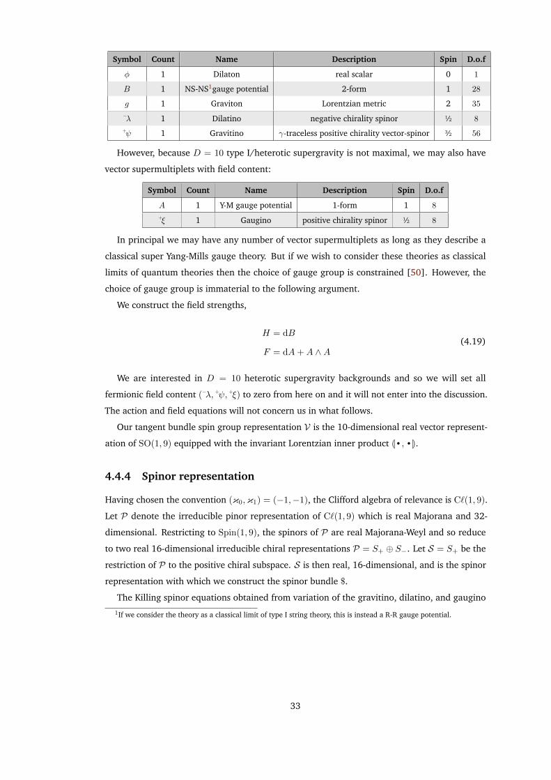
Symbol Count Name Description Spin D.o.f
φ 1 Dilaton real scalar 0 1
B 1 NS-NS1gauge potential 2-form 1 28
g 1 Graviton Lorentzian metric 2 35
−λ 1 Dilatino negative chirality spinor 1⁄2 8
+ψ 1 Gravitino γ-traceless positive chirality vector-spinor 3⁄2 56
However, because D = 10 type I/heterotic supergravity is not maximal, we may also have
vector supermultiplets with field content:
Symbol Count Name Description Spin D.o.f
A 1 Y-M gauge potential 1-form 1 8
+ξ 1 Gaugino positive chirality spinor 1⁄2 8
In principal we may have any number of vector supermultiplets as long as they describe a
classical super Yang-Mills gauge theory. But if we wish to consider these theories as classical
limits of quantum theories then the choice of gauge group is constrained [50]. However, the
choice of gauge group is immaterial to the following argument.
We construct the field strengths,
H = dB
F = dA+A ∧A(4.19)
We are interested in D = 10 heterotic supergravity backgrounds and so we will set all
fermionic field content (−λ, +ψ, +ξ) to zero from here on and it will not enter into the discussion.
The action and field equations will not concern us in what follows.
Our tangent bundle spin group representation V is the 10-dimensional real vector represent-
ation of SO(1, 9) equipped with the invariant Lorentzian inner product L·,·M.4.4.4 Spinor representation
Having chosen the convention (κ0,κ1) = (−1,−1), the Clifford algebra of relevance is C`(1, 9).
Let P denote the irreducible pinor representation of C`(1, 9) which is real Majorana and 32-
dimensional. Restricting to Spin(1, 9), the spinors of P are real Majorana-Weyl and so reduce
to two real 16-dimensional irreducible chiral representations P = S+ ⊕ S−. Let S = S+ be the
restriction of P to the positive chiral subspace. S is then real, 16-dimensional, and is the spinor
representation with which we construct the spinor bundle $.
The Killing spinor equations obtained from variation of the gravitino, dilatino, and gaugino
1If we consider the theory as a classical limit of type I string theory, this is instead a R-R gauge potential.
33

are
δψX = DXε = ∇Xε− 112 (H ·X +X ·H) · ε !
= 0 (4.20)
δλ = Pε = (dφ) · ε− 12H · ε
!= 0 (4.21)
δξ = Qε = F · ε != 0 . (4.22)
We can also write the superconnection component (equation (4.20)) as
δψX = DXε = ∇Xε− 14 ιXHε
!= 0 . (4.23)
4.4.5 Spinor inner product
We have a (Pin(1, 9)-invariant R-symplectic inner product on P induced from the hat involution
of C`(1, 9) and so equation (3.53) is satisfied.
4.4.6 Almost Killing superalgebra and homogeneity
Viewing H as an endomorphism of P, its adjoint with respect to the spinor inner product is its
image under the hat involution on C`(1, 9). The exterior algebra isomorphism sends a 3-form
to a rank-3 totally antisymmetric element of the Clifford algebra, and so it is invariant under
the hat involution. Thus H is self-adjoint as required by equation (3.54) with κ3 = −1. F does
not enter into the superconnection and so we do not worry about where it takes values, what it
does at the weekend, and why it only calls us up super early on Tuesday mornings.
We construct the squaring map as described in equation (3.22) and, choosing a pseudo-
orthonormal basis e
µ for V and corresponding gamma matrices (see appendix B.11.2) for P, the
squaring map takes the concrete form,
Ξ(ε1, ε2) = Jε1,Γµε2K e
µ = ε1Γµε2
e
µ = ε†1Γ0Γµε2
e
µ , (4.24)
where we denote the Dirac adjoint ε := ε†Γ0 .
Now, if we look at the e
0 component of a vector K = Ξ(ε, ε) obtained from the squaring map,
we see that for non-zero ε,
K0 = ε†Γ0Γ0ε = −ε†ε = −ε†ε = −|ε|2 < 0 , (4.25)
This means that a vector field K constructed by squaring a single non-zero spinor field ε is
necessarily causal because otherwise we could of course Lorentz-transform to the rest frame
where K0 = 0. Thus equation (3.55) is satisfied.
Using equation (4.50) we have for a Killing spinor ε,
∇Xε = 14 ιXH · ε . (4.26)
34
Now for a Killing vector field produced by the squaring map Kµ = Jε1,Γµε2K on two Killing
spinor fields ε1,2, we have
∇µKν = ∇µJε1,Γνε2K
= J∇µε1,Γνε2K + Jε1,Γν∇µε2K
= 18Hµρσ (JΓρσε1,Γνε2K + Jε1,ΓνΓρσε2K)
= − 18HµρσJε1, [Γ
ρσ,Γν ]ε2K
= − 12HµρσJε1,Γ
σε2K
= − 12K
σHµρσ ,
(4.27)
and thus
dK[ = −ιKH . (4.28)
Whatsmore, this means that dιKH = 0, and along with the fact that H is closed we thus have,
LKH = ιKdH + dιKH = 0 , (4.29)
whence K preserves H.
Now, using equation (4.21) we have
0 = Pε = (dφ) · ε− 12H · ε
= εPε = Jε, (dφ) · εK− 12Jε,H · εK ,
(4.30)
but the hat involution and the symmetry of the pinor inner product mean that the last term
disappears and so we have, for a Killing vector field produced by the squaring mapKµ = Jε,ΓµεK
on a single Killing spinor field,
0 = Jε, (dφ) · εK = ∇µφJε,ΓµεK = Kµ∇µφ , (4.31)
whence of course LKφ = 0 and so with the squaring map being defined by its diagonal, K
leaves φ invariant.
Now, using equation (4.22) we have
0 = Qε = F · ε
= εΓµQε = FνρJε,ΓµΓνρεK
= FνρJε,(
Γ νρµ − 2δ[ν
µ Γρ])εK ,
(4.32)
but the hat involution and the symmetry of the pinor inner product mean that the first term
disappears and so for a Killing vector field produced by the squaring map Kρ = Jε,ΓρεK on a
35
single Killing spinor field,
0 = FνρJε, δ[νµ Γρ]εK
= −2FµρJε,ΓρεK
= −2KρFµρ ,
(4.33)
whence ιKF = 0 . Then
LKF = dιKF + ιKdF = ιKdF (4.34)
and then using the Bianchi identity dF = −[A,F ] then gives,
LKF = −[ιKA,F ] , (4.35)
which is an infinitesimal gauge transformation with parameter −ιKA and so we can always
choose a gauge such that ιKA = 0 whence LKF = 0 up to gauge transformations.
Thus we have LKH = LKφ = LKF = 0 and equation (3.56) is satisfied.
We have thus satisfied all the sufficient requirements to have an almost Killing superalgebra
and for the homogeneity theorem to apply.
4.4.7 Killing superalgebra
The Fierz identity for positive chirality spinors with respect to our spinor inner product is:
εε = 116
(Jε,ΓµεKΓµ + 1
240Jε,ΓµνρστεKΓµνρστ)P(−1) , (4.36)
where P(−1) = 12 (1− Γvol) is the projector onto the negative chirality subspace.
For a Killing vector field produced by the squaring map from a single Killing spinor field,
Kµ = Jε,ΓµεK, we have
K[ · ε = Jε,Γµε,ΓKµε = ΓµεεΓµε (4.37)
and using equation (4.36),
K[ · ε = 116Γµ
(Jε,ΓνεKΓν + 1
240Jε,ΓνρστκεKΓνρστκ)P(−1)Γµε
= 116
(Jε,ΓνεKΓµΓνΓµ + 1
240Jε,ΓνρστκεKΓµΓνρστκΓµ)ε
= 116 (Jε,ΓνεK8Γν) ε = 1
2Jε,ΓνεKΓνε = 12K
[ · ε ,
(4.38)
where we have used the identities valid in ten dimensions:
ΓµΓνΓµ = 8Γν , and (4.39)
ΓµΓνρστκΓµ = 0 . (4.40)
36
Thus we clearly have that
K[ · ε = 0 . (4.41)
Now, for a Killing vector field produced by the squaring map from a single Killing spinor field,
Kµ = Jε,ΓµεK,
LKε = ∇Kε− 14 (∇K) · ε (4.42)
and using equations (4.26) and (4.28),
LKε = 14 ιKH · ε+ 1
4 ιKH · ε
= − 112K
µHνρσ (ΓνρσΓµ + ΓµΓνρσ) ε(4.43)
and using equation (4.21) on the second term,
LKε = − 112K
µHνρσΓνρσΓµε− 16K
µ(∇νφ)ΓµΓνε (4.44)
= − 112K
µHνρσΓνρσΓµε− 16K
µ(∇νφ)(−ΓνΓµ − 2δνµ1
)ε
= − 112K
µHνρσΓνρσΓµε+ 16K
µ(∇νφ)ΓνΓµε+ 13K
µ(∇µφ)1ε(4.45)
and using equation (4.31) on the last term,
LKε = − 112 (HνρσΓνρσ − 2(∇νφ)Γν)KµΓµε (4.46)
whence using equation (4.41) finally fields,
LKε = 0 . (4.47)
As such, equation (3.57) is satisfied and we have a Killing superalgebra.
4.5 D = 6, (1, 0)
4.5.1 Introduction
The homogeneity theorem and the Killing superalgebra of D = 6, (1, 0) supergravity were
described in [2] and we briefly review these constructions in our formalism. Of course, super-
symmetricD = 6, (1, 0) supergravity backgrounds are already classified [51] and either preserve
all, half, or none of the maximum supersymmetry and those that are maximally supersymmetric
are known to be homogeneous. So, although the construction of the D = 6, (1, 0) Killing super-
algebra is novel, extending it to the homogeneity theorem in this case tells us nothing new, and
we demonstrate it only for completeness.
37
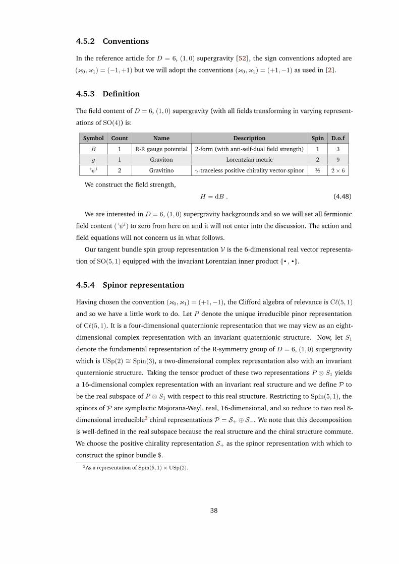
4.5.2 Conventions
In the reference article for D = 6, (1, 0) supergravity [52], the sign conventions adopted are
(κ0,κ1) = (−1,+1) but we will adopt the conventions (κ0,κ1) = (+1,−1) as used in [2].
4.5.3 Definition
The field content of D = 6, (1, 0) supergravity (with all fields transforming in varying represent-
ations of SO(4)) is:
Symbol Count Name Description Spin D.o.f
B 1 R-R gauge potential 2-form (with anti-self-dual field strength) 1 3
g 1 Graviton Lorentzian metric 2 9
+ψi 2 Gravitino γ-traceless positive chirality vector-spinor 3⁄2 2× 6
We construct the field strength,
H = dB . (4.48)
We are interested in D = 6, (1, 0) supergravity backgrounds and so we will set all fermionic
field content (+ψi) to zero from here on and it will not enter into the discussion. The action and
field equations will not concern us in what follows.
Our tangent bundle spin group representation V is the 6-dimensional real vector representa-
tion of SO(5, 1) equipped with the invariant Lorentzian inner product L·,·M.4.5.4 Spinor representation
Having chosen the convention (κ0,κ1) = (+1,−1), the Clifford algebra of relevance is C`(5, 1)
and so we have a little work to do. Let P denote the unique irreducible pinor representation
of C`(5, 1). It is a four-dimensional quaternionic representation that we may view as an eight-
dimensional complex representation with an invariant quaternionic structure. Now, let S1
denote the fundamental representation of the R-symmetry group of D = 6, (1, 0) supergravity
which is USp(2) ∼= Spin(3), a two-dimensional complex representation also with an invariant
quaternionic structure. Taking the tensor product of these two representations P ⊗ S1 yields
a 16-dimensional complex representation with an invariant real structure and we define P to
be the real subspace of P ⊗ S1 with respect to this real structure. Restricting to Spin(5, 1), the
spinors of P are symplectic Majorana-Weyl, real, 16-dimensional, and so reduce to two real 8-
dimensional irreducible2 chiral representations P = S+ ⊕ S−. We note that this decomposition
is well-defined in the real subspace because the real structure and the chiral structure commute.
We choose the positive chirality representation S+ as the spinor representation with which to
construct the spinor bundle $.
2As a representation of Spin(5, 1)×USp(2).
38
The Killing spinor equation obtained from variation of the gravitino is
δψX = DXε = ∇Xε+ 124
(H ·X[ +X[ ·H
)· ε !
= 0 , (4.49)
or equivalently using equation (B.9),
δψX = DXε = ∇Xε+ 14 ιXH · ε
!= 0 . (4.50)
4.5.5 Spinor inner product
We have a (Pin(5, 1)-invariant H-hermitian symplectic inner product on P induced from the
hat involution of C`(5, 1) and a Spin(3)-invariant H-hermitian symmetric inner product on S1
induced from the hat involution of C`(3, 0). They combine to form a (Pin(5, 1) × USp(2))-
invariant R-symplectic inner product on P (so κ3 = −1) that we will denote J·,·K. Thus
we have an R-symplectic inner product induced from the hat involution (of C`(5, 1)) and so
equation (3.53) is satisfied.
4.5.6 Almost Killing superalgebra and homogeneity
H has no USp(2) indices and so as an endomorphism of P, its adjoint with respect to the spinor
inner product is its image under the hat involution on C`(5, 1). The exterior algebra isomorphism
sends a 3-form to a rank-3 totally antisymmetric element of the Clifford algebra, and so it is
invariant under the hat involution. Thus H is self-adjoint as required by equation (3.54) with
κ3 = −1.
We construct the squaring map as described in equation (3.22) and, choosing a pseudo-
orthonormal basis e
µ for V and corresponding gamma matrices (see appendix B.11.3) for P, the
squaring map takes the concrete form,
Ξ(ε1, ε2) = Jε1,Γµε2K e
µ = ε1Γµε2
e
µ = ε†1ΓvolΓ0Γµε2
e
µ , (4.51)
where we denote the Dirac adjoint ε := ε†ΓvolΓ0 .
Now, if we look at the e
0 component of a vector K = Ξ(ε, ε) obtained from the squaring map,
we see that for non-zero ε,
K0 = ε†ΓvolΓ0Γ0ε = −ε†Γvolε = −ε†ε = −|ε|2 < 0 , (4.52)
where we have made use of the positive chirality of ε in that Γvolε = ε. This means that a
vector field K constructed by squaring a single non-zero spinor field ε is necessarily causal
because otherwise we could of course Lorentz-transform to the rest frame where K0 = 0. Thus
equation (3.55) is satisfied.
39
Using equation (4.50) we have for a Killing spinor ε,
∇Xε = − 14 ιXH · ε . (4.53)
Now for a Killing vector field produced by the squaring map Kµ = Jε1,Γµε2K on two Killing
spinor fields ε1,2, we have
∇µKν = ∇µJε1,Γνε2K
= J∇µε1,Γνε2K + Jε1,Γν∇µε2K
= − 18Hµρσ (JΓρσε1,Γνε2K + Jε1,ΓνΓρσε2K)
= 18HµρσJε1, [Γ
ρσ,Γν ]ε2K
= 12HµρσJε1,Γ
σε2K
= 12K
σHµρσ ,
(4.54)
and thus
dK[ = ιKH . (4.55)
What is more, this means that dιKH = 0, and along with the fact that H is closed we thus have,
LKH = ιKdH + dιKH = 0 , (4.56)
whence K preserves H and equation (3.56) is satisfied.
We have thus satisfied all the sufficient requirements to have an almost Killing superalgebra
and for the homogeneity theorem to apply.
4.5.7 Killing superalgebra
For a Killing vector field produced by the squaring map from a single Killing spinor field, Kµ =
Jε,ΓµεK,
LKε = ∇Kε− 14 (∇K) · ε (4.57)
and using equations (4.53) and (4.55),
LKε = − 14 ιKH · ε−
14 ιKH · ε
= − 12 ιKH · ε
= − 112
(H ·K[ +K[ ·H
)· ε .
(4.58)
40
Remembering that H is anti-self-dual, we know from appendix B.8 that H annihilates positive
chirality spinors and so
LKε = − 112H ·K
[ · ε . (4.59)
Now, the Fierz identity for positive chirality spinors with respect to our spinor inner product
is:
εε = 18
(Jε,ΓµεKΓµ + 1
12Jε,ΓµνργiεKΓµνργi)P(−1) , (4.60)
where P(−1) = 12 (1− Γvol) is the projector onto the negative chirality subspace.
Thus
K[ · ε = Jε,ΓµεKΓµε (4.61)
= εΓµεΓµε = ΓµεεΓµε
= 18Γµ
(Jε,ΓνεKΓν + 1
12Jε,ΓνρσγiεKΓνρσγi)P(−1)Γµε
= 18
(Jε,ΓνεKΓµΓνΓµ + 1
12Jε,ΓνρσγiεKΓµΓνρσΓµγi)ε
= 12Jε,ΓνεKΓνε , (4.62)
where we have used the identities valid in six dimensions:
ΓµΓνΓµ = 4Γν , and (4.63)
ΓµΓνρσΓµ = 0 . (4.64)
Comparing equation (4.61) and equation (4.62) implies thatK[ ·ε = 0 and so equation (4.59)
tells us that LKε = 0. As such, equation (3.57) is satisfied and we have a Killing superalgebra.
4.6 D = 6, (2, 0)
4.6.1 Introduction
The homogeneity theorem and the Killing superalgebra of D = 6, (2, 0) supergravity were
described in [2] and we briefly review these constructions in our formalism. Again, the con-
struction of the D = 6, (2, 0) Killing superalgebra is novel and, unlike for D = 6, (1, 0), there is
no classification of backgrounds beyond that of the maximally supersymmetric backgrounds in
[53] and so the homogeneity theorem tells us something new.
4.6.2 Conventions
For D = 6, (2, 0) supergravity [54, 55], the sign conventions adopted by [55] is (κ0,κ1) =
(−1,+1) but we will adopt the conventions (κ0,κ1) = (+1,−1) as used in [2].
41
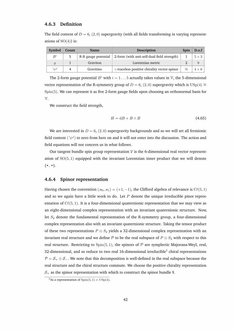
4.6.3 Definition
The field content of D = 6, (2, 0) supergravity (with all fields transforming in varying represent-
ations of SO(4)) is:
Symbol Count Name Description Spin D.o.f
Bi 5 R-R gauge potential 2-form (with anti-self-dual field strength) 1 5× 3
g 1 Graviton Lorentzian metric 2 9
+ψj 4 Gravitino γ-traceless positive chirality vector-spinor 3⁄2 4× 6
The 2-form gauge potential Bi with i = 1 . . . 5 actually takes values in V, the 5-dimensional
vector representation of the R-symmetry group of D = 6, (2, 0) supergravity which is USp(4) ∼=
Spin(5). We can represent it as five 2-form gauge fields upon choosing an orthonormal basis for
V.
We construct the field strength,
H = dB +B ∧B (4.65)
We are interested in D = 6, (2, 0) supergravity backgrounds and so we will set all fermionic
field content (+ψj) to zero from here on and it will not enter into the discussion. The action and
field equations will not concern us in what follows.
Our tangent bundle spin group representation V is the 6-dimensional real vector represent-
ation of SO(5, 1) equipped with the invariant Lorentzian inner product that we will denote
L·,·M.4.6.4 Spinor representation
Having chosen the convention (κ0,κ1) = (+1,−1), the Clifford algebra of relevance is C`(5, 1)
and so we again have a little work to do. Let P denote the unique irreducible pinor repres-
entation of C`(5, 1). It is a four-dimensional quaternionic representation that we may view as
an eight-dimensional complex representation with an invariant quaternionic structure. Now,
let S2 denote the fundamental representation of the R-symmetry group, a four-dimensional
complex representation also with an invariant quaternionic structure. Taking the tensor product
of these two representations P ⊗ S2 yields a 32-dimensional complex representation with an
invariant real structure and we define P to be the real subspace of P ⊗ S2 with respect to this
real structure. Restricting to Spin(5, 1), the spinors of P are symplectic Majorana-Weyl, real,
32-dimensional, and so reduce to two real 16-dimensional irreducible3 chiral representations
P = S+ ⊕ S−. We note that this decomposition is well-defined in the real subspace because the
real structure and the chiral structure commute. We choose the positive chirality representation
S+ as the spinor representation with which to construct the spinor bundle $.
3As a representation of Spin(5, 1)×USp(4).
42
The 3-form field strength H is V-valued and the R-symmetry group component of its action
on the spinor bundle is via the Clifford action of C`(V) ∼= C`(0, 5) on S2. This appears explicitly
in the Killing spinor equation with the gamma matrices γi the auxiliary gamma matrices of the
real Spin(5, 1)×USp(4) representation corresponding to the action of C`(0, 5) on S2.
The Killing spinor equation obtained from variation of the gravitino is
δψX = DXε = ∇Xε+ 124
(Hi ·X[ +X[ ·Hi
)· γi · ε
!= 0 , (4.66)
or equivalently using equation (B.9),
δψX = DXε = ∇Xε+ 14 ιXH
i · γi · ε!= 0 . (4.67)
4.6.5 Spinor inner product
We have a (Pin(5, 1)-invariant H-hermitian symplectic inner product on P induced from the
hat involution of C`(5, 1) and a Spin(5)-invariant H-hermitian symmetric inner product on S2
induced from the check involution of C`(0, 5). They combine to form a (Pin(5, 1) × USp(4))-
invariant R-symplectic inner product on P (so κ3 = −1) that we will denote J·,·K. Thus
we have an R-symplectic inner product induced from the hat involution (of C`(5, 1)) and so
equation (3.53) is satisfied.
4.6.6 Almost Killing superalgebra and homogeneity
H has USp(4) indices and so as an endomorphism of P, its adjoint with respect to the spinor
inner product is its image under the hat involution on C`(5, 1) and the check involution on
C`(0, 5). The exterior algebra isomorphism sends a 3-form to a rank-3 totally antisymmetric
element of the Clifford algebra, and so it is invariant under the hat involution of C`(5, 1). As
an endomorphism of C`(0, 5), H is a rank-1 element and so it is also invariant under the check
involution of C`(0, 5). Thus H is self-adjoint as required by equation (3.54) with κ3 = −1.
We construct the squaring map as described in equation (3.22) and, choosing a pseudo-
orthonormal basis e
µ for V and corresponding gamma matrices (see appendix B.11.4) for P, the
squaring map takes the concrete form,
Ξ(ε1, ε2) = Jε1,Γµε2K e
µ = ε1Γµε2
e
µ = ε†1ΓvolΓ0Γµε2
e
µ , (4.68)
where we denote the Dirac adjoint ε := ε†ΓvolΓ0 .
Now, if we look at the e
0 component of a vector K = Ξ(ε, ε) obtained from the squaring map,
we see that for non-zero ε,
K0 = ε†ΓvolΓ0Γ0ε = −ε†Γvolε = −ε†ε = −|ε|2 < 0 , (4.69)
43
where we have made use of the positive chirality of ε in that Γvolε = ε. This means that a
vector field K constructed by squaring a single non-zero spinor field ε is necessarily causal
because otherwise we could of course Lorentz-transform to the rest frame where K0 = 0. Thus
equation (3.55) is satisfied.
Using equation (4.67) we have for a Killing spinor ε,
∇Xε = − 14 ιXH
i · γi · ε. (4.70)
We define a Killing vector field produced from two Killing spinors ε1,2 via the squaring map,
Kµ = Jε1,Γµε2K , (4.71)
and then we have
∇µKν = ∇µJε1,Γνε2K
= J∇µε1,Γνε2K + Jε1,Γν∇µε2K
= − 18H
iµρσ (JΓρσγiε1,Γνε2K + Jε1,ΓνΓρσγiε2K)
= 18H
iµρσJε1, [Γ
ρσ,Γν ]γiε2K
= 12H
iµνρJε1,Γ
ργiε2K
(4.72)
Then, let us define a V-valued 1-form θ constructed from two Killing spinor fields ε1,2 via the
spinor inner product as
θiµ = Jε1,Γµγiε2K , (4.73)
which gives us4
∇µKν = 12H
iµνρθ
ρi . (4.74)
Then, pressing on, we have
∇µθiν = ∇µJε1,Γνγiε2K
= J∇µε1,Γνγiε2K + Jε1,Γνγ
i∇µε2K
= − 18H
jµρσ
(JΓρσγjε1,Γνγ
iε2K + Jε1,ΓνγiΓρσγjε2K
)= 1
8Hjµρσ
(Jγiγjε1,Γ
ρσΓνε2K− Jγjγiε1,ΓνΓρσε2K).
(4.75)
And using the relation γjγi = δij + γ i
j , and then the identity pair [Γρσ,Γν ] = 4δ[ρν Γ
σ] and
ΓρσΓν + ΓνΓρσ = 2Γρσν we have,
∇µθiν = 18H
iµρσJε1, [Γ
ρσ,Γν ]ε2K− 18H
jµρσJγ
ij ε1, (Γ
ρσΓν + ΓνΓρσ) ε2K
= 12H
iµνσJε1,Γ
σε2K + 14H
jµρσJγ
ij ε1,Γ
ρσνε2K .
(4.76)
4With an abuse of notation here, we essentially have dK[ = ιθ]H where contraction includes USp(4) indices.
44
Now, using this we can thus compute the exterior derivative of θ,
(dθ)iµν = ∇µθiν −∇νθiµ
= HiµνσJε1,Γ
σε2K + 14H
jµρσJγ
ij ε1,Γ
ρσνε2K− 1
4HjνρσJγ
ij ε1,Γ
ρσµε2K . (4.77)
We use the identity
[Γµν ,Γρστ ] = 12δ
[ρ[µΓ
στ ]ν] = 6
(δ[ρµ Γστ ]
ν − δ[ρν Γστ ]
µ
), (4.78)
to rewrite the last two terms of equation (4.77) yielding
(dθ)iµν = HiµνσJε1,Γ
σε2K + 124H
jρστ Jγ
ij ε1, [Γµν ,Γ
ρστ ]ε2K . (4.79)
As an endomorphism Γµν is in the Spin(5, 1) subalgebra of C`(5, 1) and so preserves spinor
chirality. Thus we see that Hjρστ [Γµν ,Γ
ρστ ]ε2 = 0 from the anti-self-duality of H (see ap-
pendix B.8) and the positive chirality of ε2.
We also note that the first term is precisely the contraction of Hi with a Killing vector K
constructed out of the two Killing spinors ε1,2 as defined in equation (4.71) and we thus have5
dθ = ιKH . (4.80)
This means that dιKH = 0, and along with the fact that H is closed we thus have,
LKH = ιKdH + dιKH = 0 , (4.81)
whence K preserves H and equation (3.56) is satisfied.
We have thus satisfied all the sufficient requirements to have an almost Killing superalgebra
and for the homogeneity theorem to apply.
4.6.7 Killing superalgebra
For a Killing vector field produced by the squaring map from a single Killing spinor field, Kµ =
Jε,ΓµεK,
LKε = ∇Kε− 14 (∇K) · ε (4.82)
and using equations (4.70) and (4.74),
LKε = − 18K
µHiµνρΓ
νργiε− 18θµi H
iµνρΓ
νρε
= 148H
iµνρ (ΓµνρΓσ + ΓσΓµνρ) (Kσγi + θσi ) ε .
(4.83)
5Compare this and equation (4.74).
45
Remembering that H is anti-self-dual, we know from appendix B.8 that H annihilates positive
chirality spinors and so
LKε = 148H
iµνρΓ
µνρΓσ (Kσγi + θσi ) ε (4.84)
= 148H
iµνρΓ
µνρΓσ (Jε,ΓσεKγi + Jε,ΓσγiεK) ε (4.85)
= 148H
iµνρΓ
µνρΓσ (εεΓσεγi + εεΓσγiε) (4.86)
= 148H
iµνρΓ
µνρΓσ (γiεε+ εεγi) Γσε (4.87)
Now, the Fierz identity for positive chirality spinors with respect to our spinor inner product
is:
εε = 116
(Jε,ΓµεKΓµ − Jε,ΓµγiεKΓµγi + 1
24Jε,ΓµνργijεKΓµνργij)P(−1) , (4.88)
where P(−1) = 12 (1− Γvol) is the projector onto the negative chirality subspace.
Thus, using again equations (4.63) and (4.64) we have
ΓσεεΓσε = 1
4
(Jε,ΓµεKΓµ − Jε,ΓµγjεKΓµγj
)ε , (4.89)
and so
Γσ (γiεε+ εεγi) Γσε = 14
(2Jε,ΓµεKΓµγi − Jε,ΓµγjεKΓµ(γiγ
j + γjγi))ε
= 12Γµ (Jε,ΓµεKγi + Jε,ΓµγiεK) ε .
(4.90)
Substituting equation (4.90) into equation (4.87) then yields
LKε = 196H
iµνρΓ
µνρΓσ (Jε,ΓσεKγi + Jε,ΓσγiεK) ε . (4.91)
Finally, comparing equation (4.85) and equation (4.91) implies that LKε = 0 and so equa-
tion (3.57) is satisfied and we have a Killing superalgebra.
4.7 D = 4, N = 1
4.7.1 Introduction
We construct the Killing superalgebra of D = 4, N = 1 supergravity [56, 57, 58, 59]. This
will turn out to be trivial because the lack of bosonic field content in addition to the metric
means that the superconnection is just the lift of the Levi-Civita connection and so Killing
spinors are parallel spinors whence Killing vector fields produced using the squaring map are
parallel vectors. Of course, supersymmetric D = 4, N = 1 supergravity backgrounds are already
completely classified [60] and so the homogeneity theorem in this case tells us nothing new,
and we demonstrate it only for completeness.
46
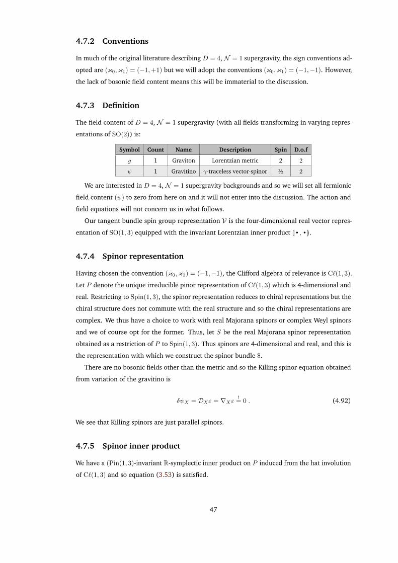
4.7.2 Conventions
In much of the original literature describing D = 4, N = 1 supergravity, the sign conventions ad-
opted are (κ0,κ1) = (−1,+1) but we will adopt the conventions (κ0,κ1) = (−1,−1). However,
the lack of bosonic field content means this will be immaterial to the discussion.
4.7.3 Definition
The field content of D = 4, N = 1 supergravity (with all fields transforming in varying repres-
entations of SO(2)) is:
Symbol Count Name Description Spin D.o.f
g 1 Graviton Lorentzian metric 2 2
ψ 1 Gravitino γ-traceless vector-spinor 3⁄2 2
We are interested in D = 4, N = 1 supergravity backgrounds and so we will set all fermionic
field content (ψ) to zero from here on and it will not enter into the discussion. The action and
field equations will not concern us in what follows.
Our tangent bundle spin group representation V is the four-dimensional real vector repres-
entation of SO(1, 3) equipped with the invariant Lorentzian inner product L·,·M.4.7.4 Spinor representation
Having chosen the convention (κ0,κ1) = (−1,−1), the Clifford algebra of relevance is C`(1, 3).
Let P denote the unique irreducible pinor representation of C`(1, 3) which is 4-dimensional and
real. Restricting to Spin(1, 3), the spinor representation reduces to chiral representations but the
chiral structure does not commute with the real structure and so the chiral representations are
complex. We thus have a choice to work with real Majorana spinors or complex Weyl spinors
and we of course opt for the former. Thus, let S be the real Majorana spinor representation
obtained as a restriction of P to Spin(1, 3). Thus spinors are 4-dimensional and real, and this is
the representation with which we construct the spinor bundle $.
There are no bosonic fields other than the metric and so the Killing spinor equation obtained
from variation of the gravitino is
δψX = DXε = ∇Xε!= 0 . (4.92)
We see that Killing spinors are just parallel spinors.
4.7.5 Spinor inner product
We have a (Pin(1, 3)-invariant R-symplectic inner product on P induced from the hat involution
of C`(1, 3) and so equation (3.53) is satisfied.
47
4.7.6 Almost Killing superalgebra and homogeneity
We have no bosonic fields in addition to the metric and so equations (3.54) and (3.56) are
automatically satisfied.
We construct the squaring map as described in equation (3.22) and, choosing a pseudo-
orthonormal basis e
µ for V and corresponding gamma matrices (see appendix B.11.5) for P, the
squaring map takes the concrete form,
Ξ(ε1, ε2) = Jε1,Γµε2K e
µ = ε1Γµε2
e
µ = ε†1Γ0Γµε2
e
µ , (4.93)
where we denote the Dirac adjoint ε := ε†Γ0 .
Now, if we look at the e
0 component of a vector K = Ξ(ε, ε) obtained from the squaring map,
we see that for non-zero ε,
K0 = ε†Γ0Γ0ε = −ε†ε = −|ε|2 < 0 , (4.94)
This means that a vector field K constructed by squaring a single non-zero spinor field ε is
necessarily causal because otherwise we could of course Lorentz-transform to the rest frame
where K0 = 0. Thus equation (3.55) is satisfied.
We have thus satisfied all the sufficient requirements to have an almost Killing superalgebra
and for the homogeneity theorem to apply.
4.7.7 Killing superalgebra
For a Killing vector field produced by the squaring map Kµ = Jε1,Γµε2K on two Killing spinor
fields ε1,2, we have
∇µKν = ∇µJε1,Γνε2K
= J∇µε1,Γνε2K + Jε1,Γν∇µε2K(4.95)
and so using equation (4.92),
∇µKν = 0 . (4.96)
Thus for a Killing vector field produced by the squaring map from a single Killing spinor field,
Kµ = Jε,ΓµεK we have
LKε = ∇Kε− 14 (∇K) · ε = 0 . (4.97)
Thus equation (3.57) is satisfied and we have a Killing superalgebra.
48
Chapter 5
Dimensional reduction of the theorem
5.1 Introduction
In chapter 4 we have shown that the strong homogeneity theorem of chapter 3 applies to a
number of a top-dimensional Poincaré supergravity theories. However, although the number of
Poincaré supergravity theories is limited, we do not care very much for demonstrating in detail
a proof of the theorem for each animal in the zoo, especially because they become more and
more unruly as the number of fields increase with dimensional reduction. Therefore we will
instead demonstrate that if we have a theory to which the strong homogeneity theorem applies,
then the strong homogeneity theorem also applies to any dimensional reduction1 of said theory.
We will begin by defining what we mean by a dimensional reduction and follow that up
by detailing the decomposition of the massless field content of a theory. Then we will discuss
the well-known fact that given a supersymmetric supergravity background, its oxidation must
preserve at least the same amount of supersymmetry. As examples, we will detail the dimensional
reductions of the Killing spinor equations of D = 11 and D = 6, (1, 0) supergravities. Finally
we will show that given a supergravity theory satisfying the strong homogeneity theorem, the
supergravity theory obtained via dimensional reduction also satisfies the strong homogeneity
theorem.
To be clear, we will be looking at a general background that upon oxidation preserves greater
than half the maximum supersymmetry and is a solution to a supergravity theory known to
satisfy the homogeneity theorem. The oxidised background is thus homogeneous, and we will
then show that this homogeneity persists after reversing the oxidation via dimensional reduction
back to the original background. The key requirement here is that the oxidation be homogeneous
as a result of the homogeneity theorem.
1As defined in section 5.2.
49

5.2 Dimensional reduction
A supergravity compactification [61, 62] is a generalisation of Kaluza-Klein theory whereby we
reduce a supergravity background in D = p + q dimensions to one in p dimensions. We start
with a supergravity background (M, g, Φ) with (M, g) a D-dimensional Lorentzian manifold and
Φ the field content of the theory. If possible, we identify an q-parameter group K of spacelike
isometries of the background, i.e. spacelike Killing vector fields ξi with LξiΦ = 0, i = 1 . . . q. We
additionally require that the action of this group is free and that the norms of ξi are nowhere
zero. This guarantees for us that the space N = M/K inherits a Lorentzian metric and via the
slice theorem is a smooth manifold. We can then view M as a principal K-bundle
K M
N
π (5.1)
whose local trivialization is the product N ×K.
At a pointm ∈M the tangent space TmM decomposes into a horizontal and vertical subspace
TmM = Hm ⊕ Vm where Vm = ker dπ and Hm = V⊥m with respect to g. This induces a
decomposition of the frame bundle structure group from SO(1, D − 1) to SO(1, p− 1)× SO(q)
and so we proceed to decompose any fields in our theory under SO(1, p−1)×SO(q) and expand
in terms of eigenfunctions of the new field-relevant differential operator Dint on K, yielding
an expanded (and possibly infinite) new set of fields. We find that the eigenvalues of these
eigenfunctions determine the mass of each of our new fields and are inversely proportional to
the length scale R of K. In the limit R→ 0 it is thus only the zero modes of the expansion that
describe the massless fields.
As supergravity is a low-energy effective field theory and R is presumed small, we are only
interested in the dynamics of massless fields and so our next step is the truncation of each
expanded field to just its zero modes. However, at this point we must be careful; such a
truncation may well not (and indeed, usually does not) satisfy our original equations of motion
because our massless modes may appear in source terms for massive modes. A consistent
truncation [63] is a compactification with truncation where any solution to the compactified,
truncated theory is also a solution of the original theory; i.e. compactification with truncation
and variation of the Lagrangian commute.
Let us consider the case where our internal manifold is a flat torus Tq. The eigenfunctions in
our field expansions are then simply the irreducible representations of U(1)q and we have one
singlet zero mode with the other modes all doublets under at least one U(1) component. If we
keep only the zero mode in our truncation then we are guaranteed it will be consistent because
singlets alone cannot act as sources for doublets2. One can also see in this specific case that
truncation is an equivalent prescription to requiring that solutions of the original theory do not
2The Noether charges of the U(1)q symmetry must be conserved.
50
depend on the coordinates of the torus. We call such a compactification where solutions have
no dependence on the coordinates of the torus a dimensional reduction.
The converse operation to dimensional reduction is oxidation. We take any solution of a
dimensionally reduced supergravity theory in p dimensions with spacetime Mp and form a
trivial fiber bundle over Mp with fiber Tq, recomposing fields accordingly to transform in the
relevant representations of SO(1, D−1). After oxidation, the new solution3 to theD-dimensional
supergravity theory has no dependence on the fiber coordinates.
We draw attention to the fact that the process of dimensional reduction is thus simply a
rewriting of equations and repackaging of degrees of freedom with oxidation the inverse pro-
cess. A small technicality is that dimensional reduction of a D-dimensional pure supergravity
background does not always result in an n-dimensional pure supergravity background. The re-
duced theory may contain extra matter multiplets. However, a p-dimensional pure supergravity
background can always be oxidised to D-dimensions.
In order to simplify the discussion, we will assume q = 1 in all that follows; i.e. dimensional
reduction and oxidation are with respect to S1 only. Thus we may adapt coordinates such that
the manifold fiber coordinate is ξ and so the spacelike vector field whose flow generates K
we denote Z = ∂ξ. Hatted objects and capitalised indices are explicitly in D dimensions, and
unhatted objects and lower-case indices explicitly in (D − 1) dimensions. Manifold indices are
Greek and flat frame indices are Latin. The frame fiber coordinate is z.
5.3 Decomposition of massless fields
Massless fields of SO(1, D−1) transform as induced representations of the little group SO(D−2).
Metric
A metric g is a rank two symmetric traceless tensor field and so transforms as the 12D(D− 3) of
SO(D − 2). It decomposes under SO(D − 3) into 12 (D− 1)(D− 4) ⊕ (D− 3) ⊕ 1, a metric g,
gauge field 1-form A, and scalar φ respectively.
Without loss of generality, the decomposition may be written in the Kaluza-Klein ansatz form
as
g = eπ∗φ(π∗g + Θ2
), (5.2)
where
Θ = Z[ + A , (5.3)
and
dA = dΘ = π∗F = π∗(dA) , (5.4)
for some 2-form F on N .3It is of course a solution because dimensional reduction is a consistent truncation.
51
Flux
For gauge fields, we are interest in invariance up to gauge transformations, and so it is the
gauge field strength that is the relevant object. A (massless) flux or field strength G is an n-form
or rank n totally antisymmetric tensor field and so transforms as the(D−2n
)of SO(D − 2). It
decomposes under SO(D−3) into(D−3n
)⊕(D−3n−1
), an n-form J and (n−1)-form H respectively.
Without loss of generality, the decomposition may be written as
G = J + Θ ∧ ιZG , (5.5)
with J a horizontal n-form on M, i.e.
ιZ J = 0 . (5.6)
Now, as a dimensional reduction we know that G is K-invariant by construction and so
0 = LZG = ιZdG+ dιZG
= LZ J + LZ ιZG = ιZdJ + Θ ∧ ιZdιZG ,(5.7)
whence
ιZdJ = ιZdιZG = 0 . (5.8)
But then LZ J = LZ ιZG = 0 and so J and ιZG are both horizontal and invariant whence they
are both basic and thus
J = π∗J , and (5.9)
ιZG = π∗H , (5.10)
for J and H an n-form and (n− 1)-form respectively on N .
Thus we have the decomposition,
G = π∗J + Θ ∧ π∗H . (5.11)
In the case where we have an (anti-)self-dual n-form, it decomposes under SO(D − 3) into
just(D−3n
), an n-form. In terms of equation (5.11) this is because H and J are Hodge-dual (up
to an appropriate sign) in D − 1 dimensions.
Vector-spinor
A (massless) gravitino is a γ-traceless vector-spinor field and so transforms as the (D− 3)2bD/2c−1
of SO(D − 2). It decomposes under SO(D − 3) into (D− 4)2b(D−1)/2c−1 ⊕ 2b(D−1)/2c−1, a
vector-spinor and spinor respectively. These fields will further decompose into chiral eigenstates
if D is odd.
52
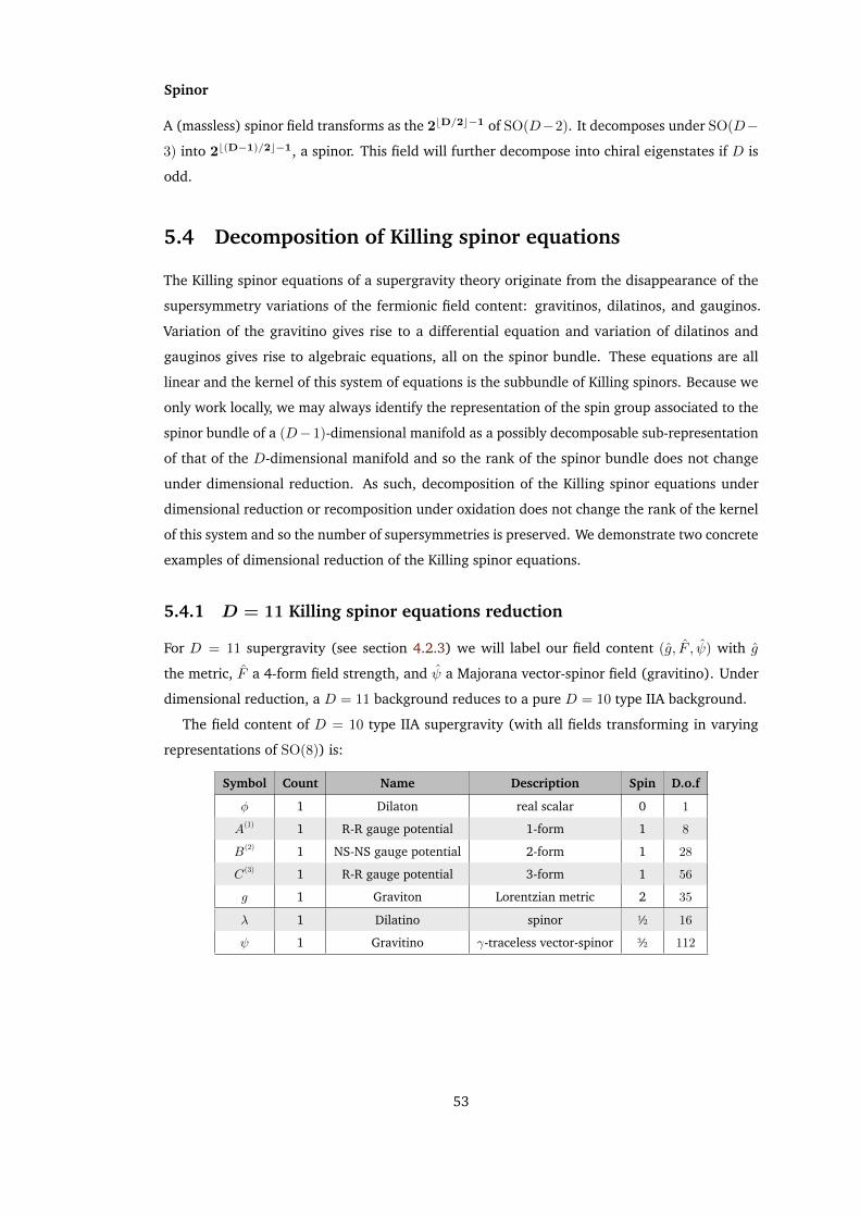
Spinor
A (massless) spinor field transforms as the 2bD/2c−1 of SO(D−2). It decomposes under SO(D−
3) into 2b(D−1)/2c−1, a spinor. This field will further decompose into chiral eigenstates if D is
odd.
5.4 Decomposition of Killing spinor equations
The Killing spinor equations of a supergravity theory originate from the disappearance of the
supersymmetry variations of the fermionic field content: gravitinos, dilatinos, and gauginos.
Variation of the gravitino gives rise to a differential equation and variation of dilatinos and
gauginos gives rise to algebraic equations, all on the spinor bundle. These equations are all
linear and the kernel of this system of equations is the subbundle of Killing spinors. Because we
only work locally, we may always identify the representation of the spin group associated to the
spinor bundle of a (D−1)-dimensional manifold as a possibly decomposable sub-representation
of that of the D-dimensional manifold and so the rank of the spinor bundle does not change
under dimensional reduction. As such, decomposition of the Killing spinor equations under
dimensional reduction or recomposition under oxidation does not change the rank of the kernel
of this system and so the number of supersymmetries is preserved. We demonstrate two concrete
examples of dimensional reduction of the Killing spinor equations.
5.4.1 D = 11 Killing spinor equations reduction
For D = 11 supergravity (see section 4.2.3) we will label our field content (g, F , ψ) with g
the metric, F a 4-form field strength, and ψ a Majorana vector-spinor field (gravitino). Under
dimensional reduction, a D = 11 background reduces to a pure D = 10 type IIA background.
The field content of D = 10 type IIA supergravity (with all fields transforming in varying
representations of SO(8)) is:
Symbol Count Name Description Spin D.o.f
φ 1 Dilaton real scalar 0 1
A(1) 1 R-R gauge potential 1-form 1 8
B(2) 1 NS-NS gauge potential 2-form 1 28
C (3) 1 R-R gauge potential 3-form 1 56
g 1 Graviton Lorentzian metric 2 35
λ 1 Dilatino spinor 1⁄2 16
ψ 1 Gravitino γ-traceless vector-spinor 3⁄2 112
53
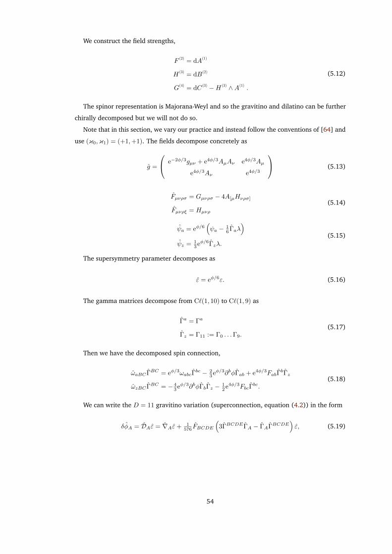
We construct the field strengths,
F (2) = dA(1)
H (3) = dB(2)
G(4) = dC (3) −H (3) ∧A(1) .
(5.12)
The spinor representation is Majorana-Weyl and so the gravitino and dilatino can be further
chirally decomposed but we will not do so.
Note that in this section, we vary our practice and instead follow the conventions of [64] and
use (κ0,κ1) = (+1,+1). The fields decompose concretely as
g =
e−2φ/3gµν + e4φ/3AµAν e4φ/3Aµ
e4φ/3Aν e4φ/3
(5.13)
Fµνρσ = Gµνρσ − 4A[µHνρσ]
Fµνρξ = Hµνρ
(5.14)
ψa = eφ/6(ψa − 1
6 Γaλ)
ψz = 13eφ/6Γzλ.
(5.15)
The supersymmetry parameter decomposes as
ε = eφ/6ε. (5.16)
The gamma matrices decompose from C`(1, 10) to C`(1, 9) as
Γa = Γa
Γz = Γ11 := Γ0 . . .Γ9.(5.17)
Then we have the decomposed spin connection,
ωaBC ΓBC = eφ/3ωabcΓbc − 2
3eφ/3∂bφΓab + e4φ/3FabΓbΓz
ωzBC ΓBC = − 43eφ/3∂bφΓbΓz − 1
2e4φ/3FbcΓbc.
(5.18)
We can write the D = 11 gravitino variation (superconnection, equation (4.2)) in the form
δφA = DAε = ∇Aε+ 1576 FBCDE
(3ΓBCDEΓA − ΓAΓBCDE
)ε, (5.19)
54
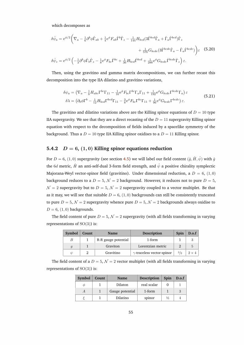
which decomposes as
δψa = eφ/2(∇a − 1
6∂bφΓab + 1
4eφFabΓbΓz − 1
144Hbcd(3ΓbcdΓa + ΓaΓbcd)Γz
+ 1576Gbcde(3ΓbcdeΓa − ΓaΓbcde)
)ε
δψz = eφ/2(− 1
3∂bφΓbΓz − 1
8eφFbcΓbc + 1
36HbcdΓbcd + 1
288eφGbcdeΓbcdeΓz
)ε.
(5.20)
Then, using the gravitino and gamma matrix decompositions, we can further recast this
decomposition into the type IIA dilatino and gravitino variations,
δψa =(∇a − 1
8HabcΓbcΓ11 − 1
16eφFbcΓbcΓaΓ11 + 1
192eφGbcdeΓbcdeΓa
)ε
δλ =(∂bφΓb − 1
12HbcdΓbcdΓ11 − 3
8eφFbcΓbcΓ11 + 1
96eφGbcdeΓbcde)ε.
(5.21)
The gravitino and dilatino variations above are the Killing spinor equations of D = 10 type
IIA supergravity. We see that they are a direct recasting of the D = 11 supergravity Killing spinor
equation with respect to the decomposition of fields induced by a spacelike symmetry of the
background. Thus a D = 10 type IIA Killing spinor oxidises to a D = 11 Killing spinor.
5.4.2 D = 6, (1, 0) Killing spinor equations reduction
For D = 6, (1, 0) supergravity (see section 4.5) we will label our field content (g, H, ψ) with g
the 6d metric, H an anti-self-dual 3-form field strength, and ψ a positive chirality symplectic
Majorana-Weyl vector-spinor field (gravitino). Under dimensional reduction, a D = 6, (1, 0)
background reduces to a D = 5, N = 2 background. However, it reduces not to pure D = 5,
N = 2 supergravity but to D = 5, N = 2 supergravity coupled to a vector multiplet. Be that
as it may, we will see that suitable D = 6, (1, 0) backgrounds can still be consistently truncated
to pure D = 5, N = 2 supergravity whence pure D = 5, N = 2 backgrounds always oxidise to
D = 6, (1, 0) backgrounds.
The field content of pure D = 5, N = 2 supergravity (with all fields transforming in varying
representations of SO(3)) is:
Symbol Count Name Description Spin D.o.f
B 1 R-R gauge potential 1-form 1 3
g 1 Graviton Lorentzian metric 2 5
ψ 2 Gravitino γ-traceless vector-spinor 3/2 2× 4
The field content of a D = 5, N = 2 vector multiplet (with all fields transforming in varying
representations of SO(3)) is:
Symbol Count Name Description Spin D.o.f
φ 1 Dilaton real scalar 0 1
A 1 Gauge potential 1-form 1 3
ξ 1 Dilatino spinor 1⁄2 4
55
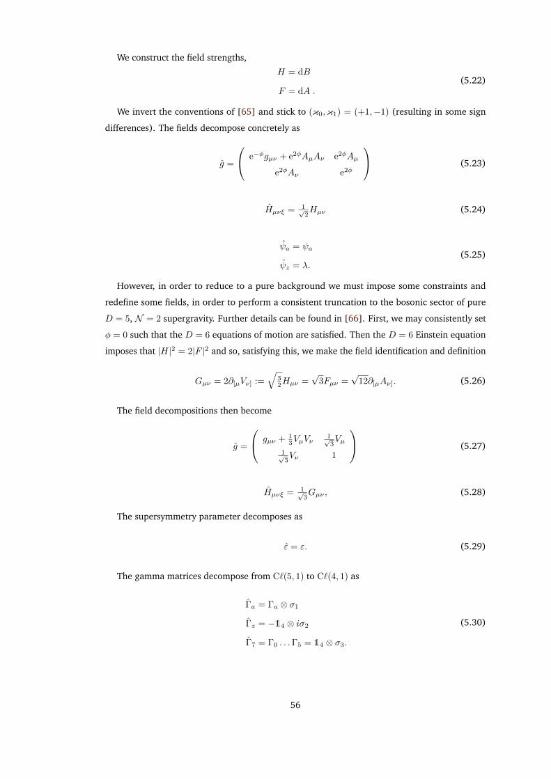
We construct the field strengths,
H = dB
F = dA .(5.22)
We invert the conventions of [65] and stick to (κ0,κ1) = (+1,−1) (resulting in some sign
differences). The fields decompose concretely as
g =
e−φgµν + e2φAµAν e2φAµ
e2φAν e2φ
(5.23)
Hµνξ = 1√2Hµν (5.24)
ψa = ψa
ψz = λ.(5.25)
However, in order to reduce to a pure background we must impose some constraints and
redefine some fields, in order to perform a consistent truncation to the bosonic sector of pure
D = 5, N = 2 supergravity. Further details can be found in [66]. First, we may consistently set
φ = 0 such that the D = 6 equations of motion are satisfied. Then the D = 6 Einstein equation
imposes that |H|2 = 2|F |2 and so, satisfying this, we make the field identification and definition
Gµν = 2∂[µVν] :=√
32Hµν =
√3Fµν =
√12∂[µAν]. (5.26)
The field decompositions then become
g =
gµν + 13VµVν
1√3Vµ
1√3Vν 1
(5.27)
Hµνξ = 1√3Gµν , (5.28)
The supersymmetry parameter decomposes as
ε = ε. (5.29)
The gamma matrices decompose from C`(5, 1) to C`(4, 1) as
Γa = Γa ⊗ σ1
Γz = −14 ⊗ iσ2
Γ7 = Γ0 . . .Γ5 = 14 ⊗ σ3.
(5.30)
56
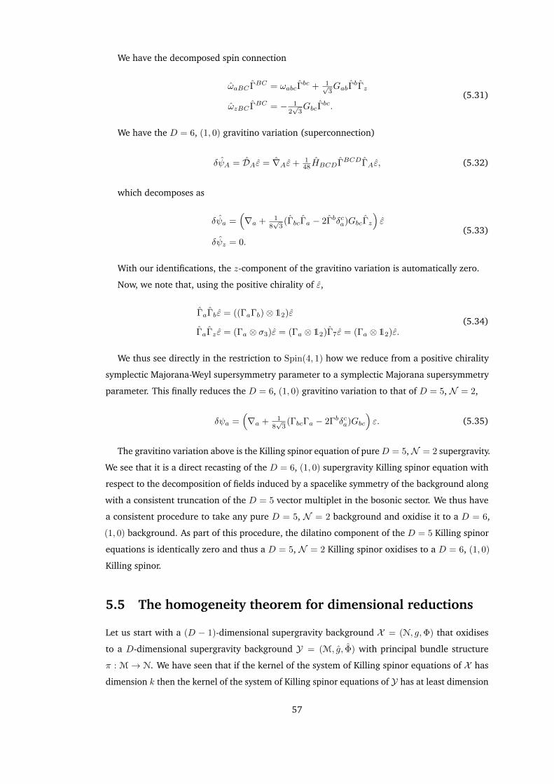
We have the decomposed spin connection
ωaBC ΓBC = ωabcΓbc + 1√
3GabΓ
bΓz
ωzBC ΓBC = − 12√
3GbcΓ
bc.(5.31)
We have the D = 6, (1, 0) gravitino variation (superconnection)
δψA = DAε = ∇Aε+ 148HBCDΓBCDΓAε, (5.32)
which decomposes as
δψa =(∇a + 1
8√
3(ΓbcΓa − 2Γbδca)GbcΓz
)ε
δψz = 0.(5.33)
With our identifications, the z-component of the gravitino variation is automatically zero.
Now, we note that, using the positive chirality of ε,
ΓaΓbε = ((ΓaΓb)⊗ 12)ε
ΓaΓz ε = (Γa ⊗ σ3)ε = (Γa ⊗ 12)Γ7ε = (Γa ⊗ 12)ε.(5.34)
We thus see directly in the restriction to Spin(4, 1) how we reduce from a positive chirality
symplectic Majorana-Weyl supersymmetry parameter to a symplectic Majorana supersymmetry
parameter. This finally reduces the D = 6, (1, 0) gravitino variation to that of D = 5, N = 2,
δψa =(∇a + 1
8√
3(ΓbcΓa − 2Γbδca)Gbc
)ε. (5.35)
The gravitino variation above is the Killing spinor equation of pureD = 5,N = 2 supergravity.
We see that it is a direct recasting of the D = 6, (1, 0) supergravity Killing spinor equation with
respect to the decomposition of fields induced by a spacelike symmetry of the background along
with a consistent truncation of the D = 5 vector multiplet in the bosonic sector. We thus have
a consistent procedure to take any pure D = 5, N = 2 background and oxidise it to a D = 6,
(1, 0) background. As part of this procedure, the dilatino component of the D = 5 Killing spinor
equations is identically zero and thus a D = 5, N = 2 Killing spinor oxidises to a D = 6, (1, 0)
Killing spinor.
5.5 The homogeneity theorem for dimensional reductions
Let us start with a (D − 1)-dimensional supergravity background X = (N, g,Φ) that oxidises
to a D-dimensional supergravity background Y = (M, g, Φ) with principal bundle structure
π : M→ N. We have seen that if the kernel of the system of Killing spinor equations of X has
dimension k then the kernel of the system of Killing spinor equations of Y has at least dimension
57
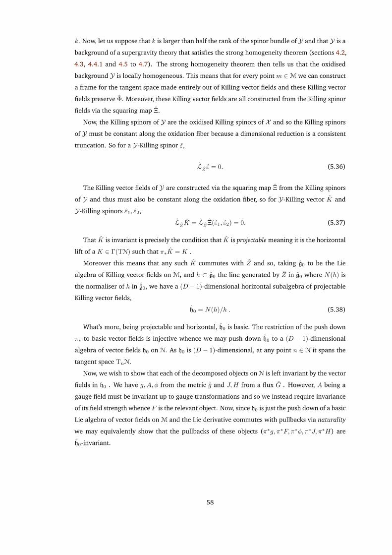
k. Now, let us suppose that k is larger than half the rank of the spinor bundle of Y and that Y is a
background of a supergravity theory that satisfies the strong homogeneity theorem (sections 4.2,
4.3, 4.4.1 and 4.5 to 4.7). The strong homogeneity theorem then tells us that the oxidised
background Y is locally homogeneous. This means that for every point m ∈M we can construct
a frame for the tangent space made entirely out of Killing vector fields and these Killing vector
fields preserve Φ. Moreover, these Killing vector fields are all constructed from the Killing spinor
fields via the squaring map Ξ.
Now, the Killing spinors of Y are the oxidised Killing spinors of X and so the Killing spinors
of Y must be constant along the oxidation fiber because a dimensional reduction is a consistent
truncation. So for a Y-Killing spinor ε,
LZ ε = 0. (5.36)
The Killing vector fields of Y are constructed via the squaring map Ξ from the Killing spinors
of Y and thus must also be constant along the oxidation fiber, so for Y-Killing vector K and
Y-Killing spinors ε1, ε2,
LZK = LZΞ(ε1, ε2) = 0. (5.37)
That K is invariant is precisely the condition that K is projectable meaning it is the horizontal
lift of a K ∈ Γ(TN) such that π∗K = K .
Moreover this means that any such K commutes with Z and so, taking g0 to be the Lie
algebra of Killing vector fields on M, and h ⊂ g0 the line generated by Z in g0 where N(h) is
the normaliser of h in g0, we have a (D − 1)-dimensional horizontal subalgebra of projectable
Killing vector fields,
h0 = N(h)/h . (5.38)
What’s more, being projectable and horizontal, h0 is basic. The restriction of the push down
π∗ to basic vector fields is injective whence we may push down h0 to a (D − 1)-dimensional
algebra of vector fields h0 on N. As h0 is (D − 1)-dimensional, at any point n ∈ N it spans the
tangent space TnN.
Now, we wish to show that each of the decomposed objects on N is left invariant by the vector
fields in h0 . We have g,A, φ from the metric g and J,H from a flux G . However, A being a
gauge field must be invariant up to gauge transformations and so we instead require invariance
of its field strength whence F is the relevant object. Now, since h0 is just the push down of a basic
Lie algebra of vector fields on M and the Lie derivative commutes with pullbacks via naturality
we may equivalently show that the pullbacks of these objects (π∗g, π∗F, π∗φ, π∗J, π∗H) are
h0-invariant.
58
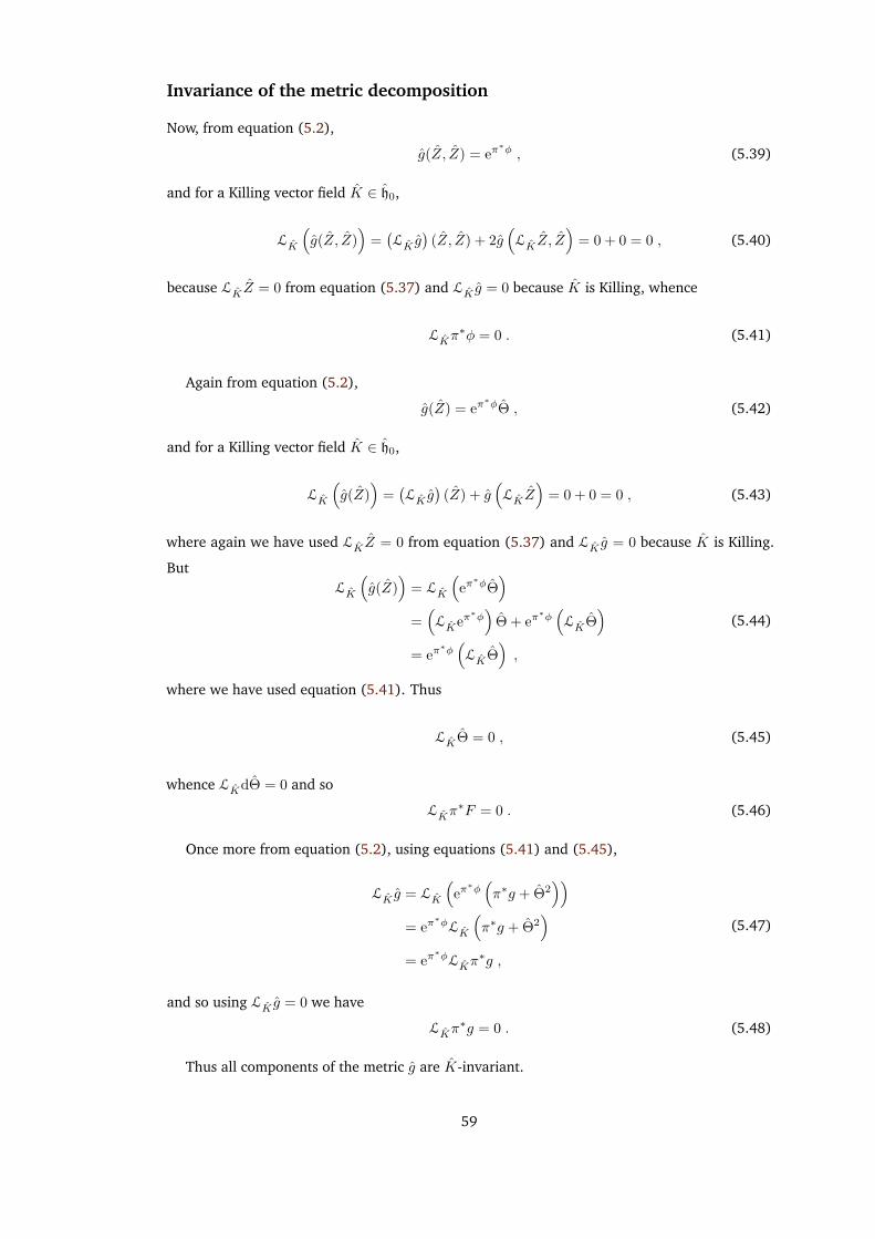
Invariance of the metric decomposition
Now, from equation (5.2),
g(Z, Z) = eπ∗φ , (5.39)
and for a Killing vector field K ∈ h0,
LK
(g(Z, Z)
)=(LK g
)(Z, Z) + 2g
(LKZ, Z
)= 0 + 0 = 0 , (5.40)
because LKZ = 0 from equation (5.37) and LK g = 0 because K is Killing, whence
LKπ∗φ = 0 . (5.41)
Again from equation (5.2),
g(Z) = eπ∗φΘ , (5.42)
and for a Killing vector field K ∈ h0,
LK
(g(Z)
)=(LK g
)(Z) + g
(LKZ
)= 0 + 0 = 0 , (5.43)
where again we have used LKZ = 0 from equation (5.37) and LK g = 0 because K is Killing.
ButLK
(g(Z)
)= LK
(eπ∗φΘ
)=(LKeπ
∗φ)
Θ + eπ∗φ(LKΘ
)= eπ
∗φ(LKΘ
),
(5.44)
where we have used equation (5.41). Thus
LKΘ = 0 , (5.45)
whence LKdΘ = 0 and so
LKπ∗F = 0 . (5.46)
Once more from equation (5.2), using equations (5.41) and (5.45),
LK g = LK
(eπ∗φ(π∗g + Θ2
))= eπ
∗φLK
(π∗g + Θ2
)= eπ
∗φLKπ∗g ,
(5.47)
and so using LK g = 0 we have
LKπ∗g = 0 . (5.48)
Thus all components of the metric g are K-invariant.
59

Invariance of the flux decomposition
For a Killing vector field K ∈ h0 we have
LKG = 0 , (5.49)
but then we have that
LK ιZG = ι[K,Z]G = 0 , (5.50)
whence from equation (5.10),
LKπ∗H = 0 . (5.51)
Now, rewriting equation (5.11) we have
π∗J = G− Θ ∧ π∗H , (5.52)
and so
LKπ∗J = LK
(G− Θ ∧ π∗H
)= 0 , (5.53)
which is clear from equations (5.45), (5.49) and (5.51).
Thus all components of the flux G are K-invariant.
We see that h0 is a Lie algebra of supergravity Killing vector fields that span the tangent space
of N and so the background X is locally homogeneous.
5.6 Conclusion
We have shown that if we have a Poincaré supergravity theory in D dimensions that has been
shown to satisfy the strong homogeneity theorem, then a theory that may be constructed as
a dimensional reduction (as defined in section 5.2) of this theory will also satisfy the strong
homogeneity theorem. This is because any background in D − 1 dimensions can be oxidised to
a background in D dimensions where the strong homogeneity theorem applies whence if the
background preserves greater than half the maximum supersymmetry, it is locally homogeneous.
Local homogeneity of the oxidised background has then been shown to imply local homogeneity
of the dimensionally reduced background. This process can be iterated and so we have shown
the strong homogeneity theorem to apply to all dimensional reductions of D = 11, 10 and
D = 6, N = 2, 4 Poincaré supergravities along with D = 4 minimal supergravity. This leaves
N = 3, 5, 6 supergravities where the strong homogeneity theorem has yet to be demonstrated.
The spectrum and coverage of Poincaré supergravity theories is shown in table 5.1.
We note that this does not mean that the dimensional reduction of any homogeneous back-
ground is again homogeneous. It also does not mean that any homogeneous background is
necessarily homogeneous upon oxidation.
60
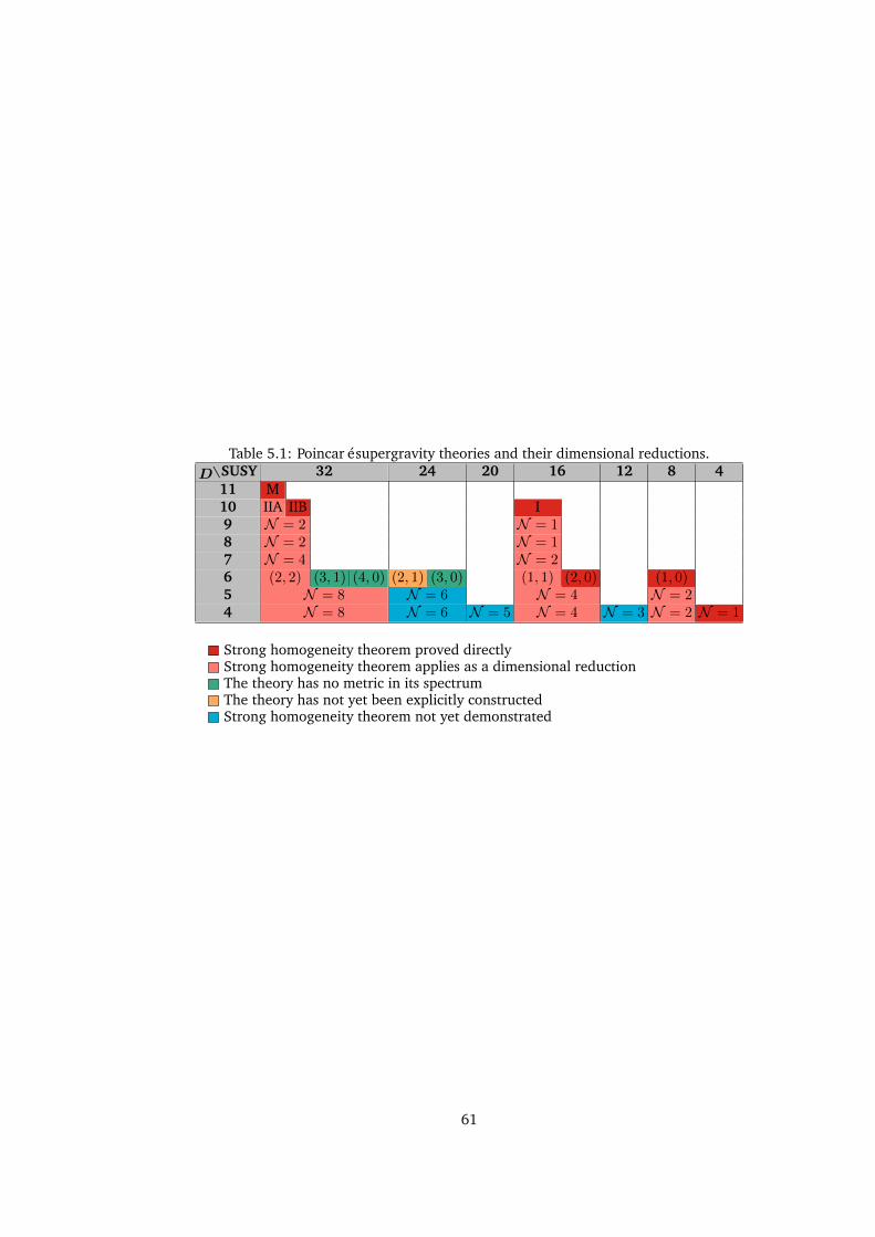
Table 5.1: Poincaré supergravity theories and their dimensional reductions.D\SUSY 32 24 20 16 12 8 4
11 M10 IIA IIB I9 N = 2 N = 18 N = 2 N = 17 N = 4 N = 26 (2, 2) (3, 1) (4, 0) (2, 1) (3, 0) (1, 1) (2, 0) (1, 0)5 N = 8 N = 6 N = 4 N = 24 N = 8 N = 6 N = 5 N = 4 N = 3 N = 2 N = 1
Strong homogeneity theorem proved directlyStrong homogeneity theorem applies as a dimensional reductionThe theory has no metric in its spectrumThe theory has not yet been explicitly constructedStrong homogeneity theorem not yet demonstrated
61
Chapter 6
Symmetric type IIB supergravitybackgrounds
6.1 Introduction
The homogeneity theorem greatly simplifies the programme of classification of supergravity
backgrounds preserving many supersymmetries. It means that in order to classify highly super-
symmetric backgrounds, we may instead classify locally homogeneous backgrounds.
However, although this is a significant improvement, we are left with the still daunting task
of classifying homogeneous backgrounds. It would seem that this will require first classifying
homogeneous Lorentzian manifolds. Progress has been achieved relatively recently in the three-
[67] and four-[68] dimensional cases and a programme in general dimensions [69, 70, 71]
has been under way for a period of time. In general dimensions, the classification of manifolds
M = G/H with semisimple G has been reduced to the case of compact stabilizer H but an
approach to classifying manifolds with non-semisimple G remains out of reach.
As such, we may be forgiven for heading straight for the low-hanging fruit: the symmetric
supergravity backgrounds. The symmetric M-theory backgrounds have been classified in [33]
and in this spirit we look to classify the symmetric backgrounds of type IIB supergravity. This
chapter is based upon work done in collaboration with José Figueroa-O’Farrill in [3].
6.2 D = 10 type IIB supergravity
D = 10 type IIB supergravity [42, 43, 44] is the low energy effective field theory of type IIB
string theory [72]. It is the unique N = (2, 0) (chiral) supergravity theory in ten dimensions
and unlike D = 10 type IIA supergravity [73, 74, 75], cannot be constructed as a dimensional
reduction of D = 11 maximal supergravity [19]. However, type IIB supergravity can be related
to type IIA supergravity through T-duality [76, 77, 78, 79] via the their common dimensional
reduction to D = 9. It has been the subject of extensive study as a tool for understanding
62
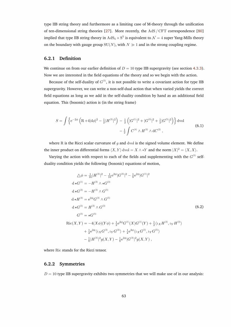
type IIB string theory and furthermore as a limiting case of M-theory through the unification
of ten-dimensional string theories [27]. More recently, the AdS /CFT correspondence [80]
implied that type IIB string theory in AdS5×S5 is equivalent to N = 4 super Yang-Mills theory
on the boundary with gauge group SU(N), with N 1 and in the strong coupling regime.
6.2.1 Definition
We continue on from our earlier definition of D = 10 type IIB supergravity (see section 4.3.3).
Now we are interested in the field equations of the theory and so we begin with the action.
Because of the self-duality of G(5), it is not possible to write a covariant action for type IIB
supergravity. However, we can write a non-self-dual action that when varied yields the correct
field equations as long as we add in the self-duality condition by hand as an additional field
equation. This (bosonic) action is (in the string frame)
S =
∫ e−2φ
(R +4|dφ|2 − 1
2 |H(3)|2)− 1
2
(|G(1)|2 + |G(3)|2 + 1
2 |G(5)|2)
dvol
− 12
∫C (4) ∧H (3) ∧ dC (2) ,
(6.1)
where R is the Ricci scalar curvature of g and dvol is the signed volume element. We define
the inner product on differential forms 〈X,Y 〉dvol = X ∧ ∗Y and the norm |X|2 = 〈X,X〉.
Varying the action with respect to each of the fields and supplementing with the G(5) self-
duality condition yields the following (bosonic) equations of motion,
4φ = 116 |H
(3)|2 − 116e2φ|G(3)|2 − 1
8e2φ|G(1)|2
d ?G(1) = −H (3) ∧ ?G(3)
d ?G(3) = −H (3) ∧G(5)
d ?H (3) = e2φG(3) ∧G(5)
d ?G(5) = H (3) ∧G(3)
G(5) = ?G(5)
Ric(X,Y ) = −4(Xφ)(Y φ) + 12e2φG(1)(X)G(1)(Y ) + 1
2 〈ιXH(3), ιYH
(3)〉
+ 12e2φ〈ιXG(3), ιYG
(3)〉+ 14e2φ〈ιXG(5), ιYG
(5)〉
− 18 |H
(3)|2g(X,Y )− 18e2φ|G(3)|2g(X,Y ) ,
(6.2)
where Ric stands for the Ricci tensor.
6.2.2 Symmetries
D = 10 type IIB supergravity exhibits two symmetries that we will make use of in our analysis:
63
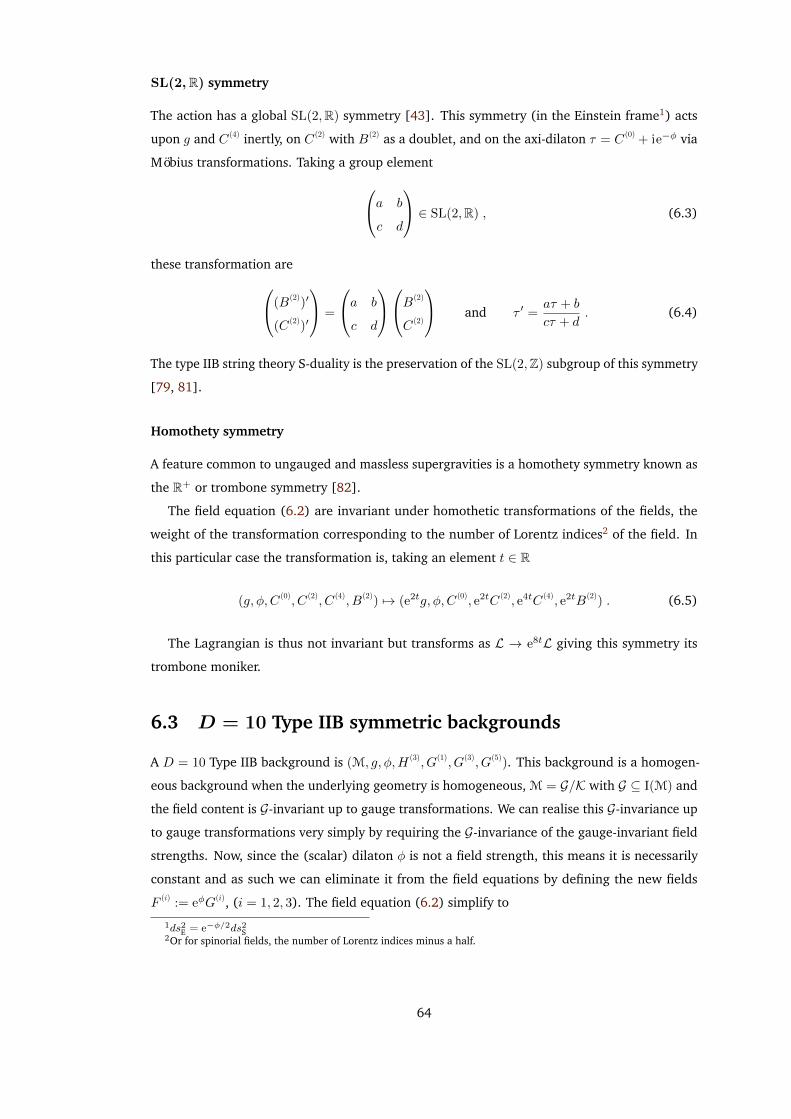
SL(2,R) symmetry
The action has a global SL(2,R) symmetry [43]. This symmetry (in the Einstein frame1) acts
upon g and C (4) inertly, on C (2) with B(2) as a doublet, and on the axi-dilaton τ = C (0) + ie−φ via
Möbius transformations. Taking a group elementa b
c d
∈ SL(2,R) , (6.3)
these transformation are(B(2))′
(C (2))′
=
a b
c d
B(2)
C (2)
and τ ′ =aτ + b
cτ + d. (6.4)
The type IIB string theory S-duality is the preservation of the SL(2,Z) subgroup of this symmetry
[79, 81].
Homothety symmetry
A feature common to ungauged and massless supergravities is a homothety symmetry known as
the R+ or trombone symmetry [82].
The field equation (6.2) are invariant under homothetic transformations of the fields, the
weight of the transformation corresponding to the number of Lorentz indices2 of the field. In
this particular case the transformation is, taking an element t ∈ R
(g, φ, C (0), C (2), C (4), B(2)) 7→ (e2tg, φ, C (0), e2tC (2), e4tC (4), e2tB(2)) . (6.5)
The Lagrangian is thus not invariant but transforms as L → e8tL giving this symmetry its
trombone moniker.
6.3 D = 10 Type IIB symmetric backgrounds
A D = 10 Type IIB background is (M, g, φ,H (3), G(1), G(3), G(5)). This background is a homogen-
eous background when the underlying geometry is homogeneous, M = G/K with G ⊆ I(M) and
the field content is G-invariant up to gauge transformations. We can realise this G-invariance up
to gauge transformations very simply by requiring the G-invariance of the gauge-invariant field
strengths. Now, since the (scalar) dilaton φ is not a field strength, this means it is necessarily
constant and as such we can eliminate it from the field equations by defining the new fields
F (i) := eφG(i), (i = 1, 2, 3). The field equation (6.2) simplify to
1ds2E = e−φ/2ds2S2Or for spinorial fields, the number of Lorentz indices minus a half.
64
|H (3)|2 = |F (3)|2 + 2|F (1)|2
d ?F (1) = ?F (3) ∧H (3)
d ?F (3) = F (5) ∧H (3)
d ?H (3) = F (3) ∧ F (5)
d ?F (5) = H (3) ∧ F (3)
F (5) = ?F (5)
Ric(X,Y ) = 12F
(1)(X)F (1)(Y ) + 12 〈ιXH
(3), ιYH(3)〉+ 1
2 〈ιXF(3), ιY F
(3)〉
+ 14 〈ιXF
(5), ιY F(5)〉 − 1
8 |H(3)|2g(X,Y )− 1
8 |F(3)|2g(X,Y ) .
(6.6)
Now, let us further specialise to the case where the underlying geometry is not only homogen-
eous but symmetric in which case we say that we have a symmetric background. For a symmetric
space we have that any invariant n-form A(n) is parallel with respect to the canonical connection
(see section 2.2.1) which is the Levi-Civita connection (∇A(n) = 0) and so its dual ?A(n) is also
parallel (∇ ?A(n) = 0) whence it is both closed (dA(n) = 0) and co-closed (d ?A(n) = 0). The field
equations then further simplify to
|H (3)|2 = |F (3)|2 + 2|F (1)|2 (6.7)
0 = ?F (3) ∧H (3) (6.8)
0 = F (5) ∧H (3) (6.9)
0 = F (3) ∧ F (5) (6.10)
0 = H (3) ∧ F (3) (6.11)
F (5) = ?F (5) (6.12)
Ric(X,Y ) = 12F
(1)(X)F (1)(Y ) + 18
(4〈ιXH (3), ιYH
(3)〉 − |H (3)|2g(X,Y ))
+ 18
(4〈ιXF (3), ιY F
(3)〉 − |F (3)|2g(X,Y ))
+ 14 〈ιXF
(5), ιY F(5)〉 .
(6.13)
Now, using the classification and enumeration of Lorentzian symmetric spaces described in
section 2.2.2, we can take a particular Lorentzian symmetric space M = M0 ×M1 × . . .×Mn,
where each factor determined by its Lie algebra pair (k,m)i, along with the set of k-invariant
forms for each factor.
Using the correspondence in equation (2.10) we then algebraise the field equations (6.7)
to (6.13). For each field strength n-form (evaluated at the origin), we construct the most general
possible (real-)parametrised ansatz k-invariant n-form out of the the set of available k-invariant
forms on our factors, with F (1) ∈ mk, F (3), H (3) ∈ (Λ3m)k, and F (5) ∈ (Λ5+m)k. Substituting in
these ansatz field strengths to the algebraised field equations yields a system of polynomial
equations in the parameters of the ansätze whose solution space is the moduli space of the
65
background.
6.4 Classification of Type IIB backgrounds
6.4.1 Organisation
In section 6.4.2 we make some general observations that will aid us in understanding and
computing moduli spaces. In section 6.4.3 we lay out the notation we will use unless otherwise
stated. We then make a start in section 6.4.4 by ruling out whole classes of backgrounds based
on general arguments. In section 6.4.5 we list geometries that have been individually ruled out
and explain or give reference for the arguments used. Then in sections 6.4.6 to 6.4.9 we list
those geometries for which we have found solutions3. Finally in section 6.4.10 we summarise
our results.
6.4.2 Observations
Interchangeability of invariant forms
When computing the existence and moduli space of backgrounds, the spaces in each of the
pairs (S5,SLAG3), (CP3,G+R (2, 5)), and (HP2,ASSOC) are interchangeable because they have
the same invariant forms which can also be identically normalised.
The existence of a background with a Sn factor implies the existence of backgrounds with the
Sn factor replaced by any other n-dimensional possibly reducible compact (non-flat) Riemannian
factor. Similarly the existence of a background with an AdSn factor implies the existence of
backgrounds with the AdSn factor replaced by AdSp×Mn−p where Mn−p is a possibly reducible
non-compact (non-flat) Riemannian factor. This is due to the fact that invariant forms for Sn
and AdSn factors are nothing but multiples of their volume forms and so can be substituted by
the volume forms of the possibly reducible factors that replace them with no effect. Note that
this argument clearly does not work in reverse!
Residual SO(2) symmetry
When F (1) = 0 we have that C (0) is constant and then so is the axi-dilaton τ = C (0) + ie−φ.
We may thus use the SL(2,R) symmetry of the field equations described in section 6.2.2 to
transform the axi-dilaton to τ = i. The subgroup of SL(2,R) that stabilises τ = i is SO(2) and
so any background that has non-zero H (3) or F (3) and τ = i will correspond to an SO(2) orbit
of backgrounds. So, when we have a backgrounds with F (1) = 0 and non-zero H (3) and F (3), we
may use this residual SO(2) symmetry acting as rotations on the (H (3),F (3)) plane to simplify
3Some of those solutions will have flatness forced on one or more of the factors and thus will not be a solution forthe original geometry. An example is AdS3 × S4 × S3.
66
the background as a representative of the SL(2,R) orbit. A demonstrative example where we
do this can be found in section 6.4.8.
Limit solutions
If we have an exactly solved moduli space for a particular background, we may see that in
certain limits [36] we recover a different background, with one or more factors of the original
geometry becoming flat. In this way we can see that certain backgrounds must exist even if we
cannot compute their entire moduli space.
Polynomial systems
Parametrisation
We are working with geometries that are products of a number of factors. When we construct
the most general invariant n-form for a particular product geometry, it is a parametrised sum
of all the possible independent n-forms constructed from the invariant forms of the factors.
When we substitute this most general form into the field equations it reduces to a system of
polynomial equations in said parameters. We then add further constraints into the system based
on geometrical considerations, such as requiring that Ricci-flat and non-Ricci-flat have vanishing
and non-vanishing Ricci tensors respectively through the Einstein equation.
A given geometry will have spaces of invariant 1-forms, 3-forms, and self-dual 5-forms of
dimensions m1 = dimmk, m3 = dim(Λ3m
)kand m+
5 = dim(Λ5
+m)k
, respectively. This gives us
a total of m1 + 2m3 +m+5 parameters which are then constrained by the field equations to form
the moduli space.
Reduction via symmetries
If F (1) = 0, we may use the SO(2) stabiliser subgroup of the SL(2,R) symmetry to eliminate
one of the 3-form parameters (the parameters that we later call αi, βj) to give a representative
background of an SL(2,R) orbit of backgrounds as described in section 6.4.2. We might then
also use the homothety invariance described in section 6.2.2 to eliminate one parameter if it
helps us to simplify things. Solving this final system gives us the moduli space of the background.
Numerical solutions
We desire in all cases to solve analytically for the moduli space and in most cases it is possible
to solve this polynomial system over the reals. However, in some cases the system becomes
unwieldy and an analytical solution is no longer computationally possible [83]. In such cases,
we resort to a search for numerical solutions.
Our technique is blunt: we take the sum of the squares of our normalised polynomial system
F =∑i f
2i and then use a low discrepancy quasi-random sampling of the homothetically
67
compactified solution space of our system as seeds for standard numerical minimisation routines
applied to F . We accept local minima as valid solutions as long as |F | < 10−30. Note that
calculations were carried out with a working precision of 10−60. Checks using the application
of this technique to the polynomial systems that were analytically solvable were encouraging.
However, a pinch of salt is prescribed.
We applied this technique in two ways to help us with difficult polynomial systems. First, to
trawl the solution space of a system to hint at whether solutions may exist and if so, to indicate
the (non-)compactness of factor geometries. Second, and when solutions are suggested to exist,
to present potential ansätze for finding exact solutions.
In some cases, where the moduli space of a background is too complicated to solve exactly,
we may have already seen the background as a limit of the moduli space of another background
as explained in section 6.4.2. In these cases, we may not even look for numerical solutions
because there is nothing further to gain. In particular, by considering the balance of curvatures
between factors, we know that we do not miss any non-compact factor geometries by doing this.
6.4.3 Notation
We will use the following notation throughout this section:
Symbol Description
A(n) Any invariant n-form composed of components only from the Lorent-
zian symmetric space factor. The rank of the form will be omitted if it
is clear from the context. The form may be trivial.
A(n) Any invariant n-form composed of components only from the Rieman-
nian symmetric space factor. The rank of the form will be omitted if it
is clear from the context. The form may be trivial.
ν0 The volume form on the Lorentzian symmetric space factor
νi The volume form on the ith Riemannian symmetric space factor
dϑi The volume form on the ith Riemannian flat factor. The index is
suppressed when there is only one flat factor.
dϑ123... A composite Riemannian flat factor volume form, dϑ1∧dϑ2∧dϑ3∧ . . .
X , Y , . . . Vector fields tangent to the Lorentzian symmetric space factor
X,Y , . . . Vector fields tangent to the Riemannian symmetric space factor
g0 The metric on the Lorentzian symmetric space factor
gi The metric on the ith Riemannian symmetric space factor
g The metric on the Riemannian symmetric space factor
68
λ, α, β, κ Real parameters with (generally) λ parametrising F (1), α paramet-
rising H (3), β parametrising F (3), and κ parametrising F (5)
Ri The Ricci scalar curvature on the ith factor (i = 0 Lorentzian, i > 0
Riemannian)
6.4.4 Special Cases
de Sitter backgrounds
We analyse backgrounds of the form dSd×M10−d for d ≥ 2. The most general 5-form we can
construct takes the form
F (5) = ν (d)0 ∧ τ
(5− d)5 + F (5) , (6.14)
whence
〈ιXF (5), ιY F(5)〉 = 〈ιX ν (d)
0 , ιY ν(d)0 〉|τ
(5− d)5 |2 = −|τ (5− d)
5 |2g(X,Y ) . (6.15)
The most general 3-form we can construct (K standing for H (3) or F (3)) takes the form
K (3) = ν (d)0 ∧ τ
(3− d)K +K (3) , (6.16)
whence
〈ιXK (3), ιY K(3)〉 = 〈ιX ν (d)
0 , ιY ν(d)0 〉|τ
(5− d)K |2 = −|τ (5− d)
K |2g(X,Y ) , and (6.17)
|K (3)|2 = |ν (d)0 |2|τ
(3− d)K |2 + |K (3)|2 = −|τ (3− d)
K |2 + |K (3)|2 , (6.18)
so
4〈ιXK (3), ιY K(3)〉 − |K (3)|2g(X,Y ) = −
(3|τ (5− d)
K |2 + |K (3)|2)g(X,Y ) . (6.19)
Finally, since dSd has no invariant 1-forms,
F (1)(X )F (1)(Y ) = 0 . (6.20)
Therefore, the Einstein equation equation (6.13) on the de Sitter factor is
Ric(X,Y ) = − 18
(3|τ (3− d)
H |2 + 3|τ (3− d)F |2 + 2|τ (5− d)
5 |2 + |H (3)|2 + |F (3)|2)g(X,Y ) . (6.21)
We notice that this implies a negative-semidefinite curvature contradicting the fact that dSd has
positive curvature. As such, this rules out all backgrounds with a de Sitter factor. Since we only
used the Einstein equation (which was not simplified from equation (6.6) to equation (6.13))
this is true in general for homogeneous backgrounds and not only symmetric ones.
69
Backgrounds with a 1-dimensional Lorentzian factor
We analyse backgrounds of the form R0,1×M9 for d ≥ 2, i.e. with metric of the form g = −dt2+g ,
and define T to be a vector field tangent to the R0,1 factor.
The most general 5-form we can construct takes the form
F (5) = ν0 ∧ τ (4)5 + F (5) , (6.22)
whence
〈ιTF (5), ιTF(5)〉 = −|τ (4)
5 |2g(T, T ) = |τ (4)5 |2 . (6.23)
The most general 3-form we can construct (K standing for H (3) or F (3)) takes the form
K (3) = ν0 ∧ τ (2)K +K (3) , (6.24)
whence
〈ιTK (3), ιTK(3)〉 = −|τ (2)
K |2g(T, T ) = |τ (2)K |2 , and (6.25)
|K (3)|2 = |K (3)|2 − |τ (3)K |2 , (6.26)
so
4〈ιTK (3), ιTK(3)〉 − |K (3)|2g(T, T ) = 3|τ (2)
K |2 + |K (3)|2 . (6.27)
For F (1), we have the most general form
F (1) = αdt+ F (1) , (6.28)
whence
F (1)(T )F (1)(T ) = α2 (6.29)
Therefore, the Einstein equation equation (6.13) on the −dt2 factor is
Ric(T, T ) = 18
(4α2 + 3|τ (2)
H |2 + 3|τ (2)F |2 + 2|τ (4)
5 |2 + |H (3)|2 + |F (3)|2). (6.30)
This factor is flat and so the Ricci curvature on the factor must be identically zero. All the terms
are positive-semidefinite being either a squared real parameter or the squared norms of purely
Riemannian forms. Thus F (1), H (3), and F (3) are all zero and we are left with F (5) = F (5) since
this component does not contribute to the curvature. However, F (5) is self-dual and a self-dual
form has zero norm so
0!= |F (5)|2 = |F (5)|2 , (6.31)
whence F (5) is also forced to be zero. Therefore we have F (1) = H (3) = F (3) = F (5) = 0. This
means that g is Ricci-flat and hence flat and so locally isometric to the Minkowski vacuum. Again,
70
since we only used the Einstein equation this is true in general for homogeneous backgrounds
and not only symmetric ones.
Cahen-Wallach backgrounds
We analyse backgrounds with metric of the form CWd(λ) ×M10−d. The most general n-form
we can construct takes the form
W (n) = ν (d)0 ∧W
(n− d)1 +W (n)
2 +∑i
τ (si)i ∧ Z
(n− si)i , (6.32)
where the first term is the wedge product of the Cahen-Wallach volume form with an invariant
form on the Riemannian factors, the second term is an invariant form on the Riemannian factors,
and the third term is a sum of wedge products of Cahen-Wallach non-volume invariant forms and
invariant forms on the Riemannian factors. Using the fact that all Cahen-Wallach non-volume
invariant forms are null and so |τ (si)i |2 = 0, we have
〈ιXW(n), ιYW
(n)〉 = −〈ιXW(n− d)1 , ιYW
(n− d)1 〉+ 〈ιXW
(n)2 , ιYW
(n)2 〉 , (6.33)
〈ιXW (n), ιYW(n)〉 = −|W (n− d)
1 |2g(X,Y ) , and (6.34)
|W (n)|2 = −|W (n− d)1 |2 + |W (n)
2 |2 , (6.35)
so
4〈ιXW (n), ιYW(n)〉 − |W (n)|2g(X,Y ) = −
(3|W (n− d)
1 |2 + |W (n)2 |2
)g(X,Y ) . (6.36)
Therefore, the Einstein equation equation (6.13) on the Cahen-Wallach factor is
Ric(X,Y ) = − 18
(3|H (3− d)
1 |2 + 3|F (3− d)1 |2 + 2|F (5− d)
1 |2 + |H (3)2 |2 + |F (3)
2 |2)g(X,Y ) . (6.37)
Cahen-Wallach spaces are Ricci-null and so the Ricci curvature on this factor must be identically
zero. All the terms are negative-semidefinite and so each term is forced to zero. In particular,
this means that |H (3)|2 = |F (3)|2 = 0 whence equation (6.7) tells us that |F (1)|2 = 0. Since there
can be no F (1− d)1 component on dimensional grounds, this means that |F (1)
2 |2 = 0 and so F (1)2 = 0.
From self-duality we have |F (5)|2 = 0 and since |F (5− d)1 |2 = 0, this means that |F (5− d)
2 |2 = 0 and
so F (5− d)2 = 0. Thus H (3), F (1), F (3), and F (5) all take the form of equation (6.32) where the first
two terms are absent. But then, equation (6.33) tells us that they do not contribute to the Ricci
tensor of the Riemannian factor either, which is then forced to be Ricci-flat and so flat. We are
thus left with only CWd(λ)× R10−d.
High-dimensional factors
9-dimensional irreducible Riemannian factors
These are the cases already dealt with in section 6.4.4.
71
8-dimensional irreducible Riemannian factors
• (su(3)⊕ su(3), su(3)) and (sl(3,C), su(3)):
The only available complementary space is AdS2. We have a single invariant 3-form
and there are no available invariant 1-forms so the field equations (6.7) to (6.9) dictate
F (1) = H (3) = F (3) = 0. The most general self-dual 5-form is
F (5) = κ(ν0 ∧ τ (3) − τ (5)) . (6.38)
With the equations of motion thus satisfied, the Einstein equation then yields
R0 = − 14κ
2g0 and R1 = 116κ
2g1 , (6.39)
which gives a solution for the compact case AdS2×SU(3).
• Other 8-dimensional Riemannian factors:
The only available complementary space is AdS2. As such there are no invariant 3-forms
or 5-forms and so Ricci-flatness is forced. However, these spaces are not Ricci-flat and so
we have a contradiction with the negative curvature of AdS2 and thus these spaces are
ruled out.
7-dimensional irreducible Riemannian factors
The only 7-dimensional Riemannian factor is S7. We have no invariant 1-forms or 5-forms
in the Riemannian part and only the invariant 3-form of the Lorentzian volume. Thus the
field equations (6.7) to (6.9) dictate H (3) = F (3) = F (1) = 0 which forces Ricci-flatness, again
contradicting the curvature of AdS3 and thus these spaces are ruled out.
AdSd>7 backgrounds
In this case there are no invariant 3-forms or invariant 5-forms and so the Einstein equation
forces Ricci-flatness, again contradicting the curvature of AdSd>7 and thus these spaces are
ruled out.
6.4.5 Individually inadmissible geometries
Here we list the geometries not already ruled out by general arguments but which we have
shown to not admit any solutions. Although we list the geometries by using the compact version
of the Riemannian symmetric spaces, their non-compact duals are similarly ruled out.
72
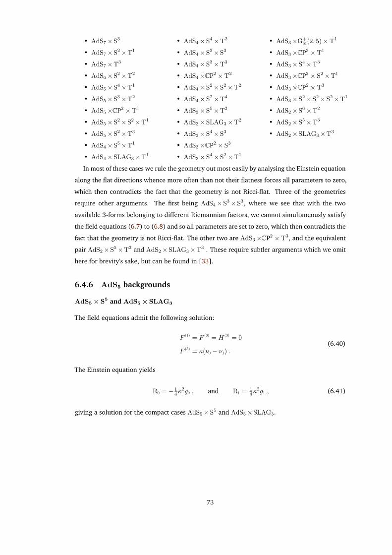
• AdS7×S3
• AdS7×S2×T1
• AdS7×T3
• AdS6×S2×T2
• AdS5×S4×T1
• AdS5×S3×T2
• AdS5×CP2 × T1
• AdS5×S2×S2×T1
• AdS5×S2×T3
• AdS4×S5×T1
• AdS4×SLAG3×T1
• AdS4×S4×T2
• AdS4×S3×S3
• AdS4×S3×T3
• AdS4×CP2 × T2
• AdS4×S2×S2×T2
• AdS4×S2×T4
• AdS3×S5×T2
• AdS3×SLAG3×T2
• AdS3×S4×S3
• AdS3×CP2 × S3
• AdS3× S4×S2×T1
• AdS3×G+R (2, 5)× T1
• AdS3×CP3 × T1
• AdS3×S4×T3
• AdS3×CP2 × S2×T1
• AdS3×CP2 × T3
• AdS3×S2×S2×S2×T1
• AdS2×S6×T2
• AdS2×S5×T3
• AdS2×SLAG3×T3
In most of these cases we rule the geometry out most easily by analysing the Einstein equation
along the flat directions whence more often than not their flatness forces all parameters to zero,
which then contradicts the fact that the geometry is not Ricci-flat. Three of the geometries
require other arguments. The first being AdS4×S3× S3, where we see that with the two
available 3-forms belonging to different Riemannian factors, we cannot simultaneously satisfy
the field equations (6.7) to (6.8) and so all parameters are set to zero, which then contradicts the
fact that the geometry is not Ricci-flat. The other two are AdS3×CP2 × T3, and the equivalent
pair AdS2×S5×T3 and AdS2× SLAG3×T3 . These require subtler arguments which we omit
here for brevity’s sake, but can be found in [33].
6.4.6 AdS5 backgrounds
AdS5×S5 and AdS5× SLAG3
The field equations admit the following solution:
F (1) = F (3) = H (3) = 0
F (5) = κ(ν0 − ν1) .(6.40)
The Einstein equation yields
R0 = − 14κ
2g0 , and R1 = 14κ
2g1 , (6.41)
giving a solution for the compact cases AdS5×S5 and AdS5×SLAG3.
73
AdS5×S3×S2
The field equations admit the following solution:
F (1) = F (3) = H (3) = 0
F (5) = κ(ν0 − ν1 ∧ ν2) .(6.42)
The Einstein equation yields
R0 = − 14κ
2g0 , R1 = 14κ
2g1 , and R2 = 14κ
2g2 , (6.43)
giving a solution for the compact case AdS5×S3×S2. The existence of this background follows
from the existence of the AdS5×S5 background via the argument in section 6.4.2.
6.4.7 AdS4 backgrounds
AdS4×S3×S2×T1
The field equations admit the following solution, with ξi = ±1:
F (1) = λdϑ
F (3) = 0
H (3) = ξ1√
2λν2 ∧ dϑ
F (5) = ξ2√
5λ(ν0 ∧ dϑ + ν1 ∧ ν2) .
(6.44)
The Einstein equation yields
R0 = − 32λ
2g0 , R1 = λ2g1 , and R2 = 2λ2g2 , (6.45)
giving a solution for AdS4×S3×S2×T1.
6.4.8 AdS3 backgrounds
For AdS3 and AdS2 the moduli spaces become increasingly difficult to compute as the number
of 3-form components increases, and even when computed may be difficult to interpret.
AdS3×S5×S2 and AdS3× SLAG3× S2
The field equations admit the following solution:
F (1) = F (3) = H (3) = 0
F (5) = κ(ν1 − ν0 ∧ ν2) .(6.46)
74
The Einstein equation yields:
R0 = − 14κ
2g0 , R1 = 14κ
2g1 , and R2 = − 14κ
2g2 , (6.47)
giving a solution for the cases AdS3× S5×H2 and AdS3×SLAG3×H2. We could have deduced
the existence of such a background from that of the AdS5×S5 background via the argument in
section 6.4.2.
AdS3×S4×S3
The field equations admit the following solution with ξ = ±1:
F (1) = F (5) = 0
F (3) = β(ν0 + ξν2)
H (3) = α(ν0 + ξν2) .
(6.48)
As explained in section 6.4.2, there is a residual SO(2) subgroup of the SL(2,R) symmetry group
which we may use to simplify the solution further. This subgroup acts by rotations on (F (3), H (3))
or, equivalently here, on (α, β). Thus we will use this to set β = 0, whence the simplified
solution as a representative of the SL(2,R) orbit is:
F (1) = F (3) = F (5) = 0
H (3) = α(ν0 ± ν2) .(6.49)
The Einstein equation yields:
R0 = − 12α
2g0 , R1 = 0, and R2 = 12α
2g2 . (6.50)
As R1 = 0 is forced, this geometry is ruled out and what we actually obtain is a background with
underlying geometry AdS3×T4×S3.
AdS3×CP2 × S3
The field equations admit the following solution with ω the Kähler form in the Hermitian
symmetric space CP2, ξ = ±1, and where we have used the residual SO(2) symmetry to set
F (3) = 0:
F (1) = F (3) = 0
H (3) = α(ν0 + ξν2)
F (5) = 12 (1 + ξ)κ(ν0 + ξν2) ∧ ω .
(6.51)
75
The Einstein equation then yields:
R0 = − 12 (α2 + κ2)g0 , R1 = 0, and R2 = 1
2 (α2 + κ2)g2 . (6.52)
As R1 = 0 is forced, this geometry is ruled out and what we actually obtain is a background with
underlying geometry AdS3×T4×S3.
AdS3×S3×S2× S2
The field equations admit the following two branches of solutions with ξ = ±1:
1.F (1) = F (3) = H (3) = 0
F (5) = κ1(ν0 ∧ ν2 − ν1 ∧ ν3) + κ2(ν0 ∧ ν3 − ν1 ∧ ν2) .(6.53)
The Einstein equation then yields:
R0 = − 14 (κ2
1 + κ22)g0 , R1 = 1
4 (κ21 + κ2
2)g1 ,
R2 = − 14 (κ2
1 − κ22)g2 , and R3 = 1
4 (κ21 − κ2
2)g3 ,(6.54)
which gives a solution for AdS3×S3×S2×H2. This solution degenerates to a solution for
AdS3× S3×T4 when κ21 = κ2
2.
The existence of the special case κ1 = 0 of this background follows from the AdS5× S5
background via the argument in section 6.4.2.
2.F (1) = F (3) = 0
H (3) = α(ν0 + ξν1)
F (5) = κ(ν0 − ν1) ∧ (ν2 − ξν3) .
(6.55)
The Einstein equation then yields:
R0 = − 12 (α2 + κ2)g0 , R1 = 1
2 (α2 + κ2)g1 , and R2 = R3 = 0 . (6.56)
As R2 = R3 = 0 is forced, what we actually obtain is a solution for AdS3×S3×T4.
AdS3×S3×S3×T1
The field equations admit the following solution:
F (1) = F (5) = 0
F (3) = β1ν0 + β2ν1 + β3ν2
H (3) = α1ν0 + α2ν1 + α3ν2 ,
(6.57)
76
withα2
1 = α22 + α2
3, β21 = β2
2 + β23 , α1β2 = β1α2,
α1β3 = β1α3, and α2β3 = β2α3 .(6.58)
The last three equations say that the vectors (α1, α2, α3) and (β1, β2, β3) are collinear, so
that F (3) and H (3) point in the same direction. In this case we can then use the residual SO(2)
symmetry to set the βi = 0, whence we arrive at the simplified solution:
F (1) = F (3) = F (5) = 0
H (3) = α1ν0 + α2ν1 + α3ν2 ,(6.59)
with
α21 = α2
2 + α23 . (6.60)
The Einstein equation then yields:
R0 = − 12α
21g0 , R1 = 1
2α22g1 , and R2 = 1
2α23g2 , (6.61)
giving a solution for AdS3×S3×S3×T1. This solution degenerates to one for AdS3×S3×T4
whenever α2 = 0 or α3 = 0.
AdS3×S3×S2×T2
The field equations admit the following two branches of solutions with ξi = ±1:
1.F (1) = 0
F (3) = ξ1
√κ2
2 − κ21ν2 ∧ dϑ2
H (3) = ξ2
√κ2
2 − κ21ν2 ∧ dϑ1
F (5) = (κ1ν0 + κ2ν1) ∧ ν2 − (κ2ν0 + κ1ν1) ∧ dϑ1 ∧ dϑ2 .
(6.62)
The Einstein equation then yields:
R0 = − 12κ
22g0 , R1 = 1
2κ21g1 , and R2 = (κ2
2 − κ21)g2 , (6.63)
giving a solution for the compact case AdS3×S3×S2×T2. This solution degenerates to
one for AdS3×S3×T4 if κ21 = κ2
2, and to one for AdS3× S2×T5 if κ21 = 0.
2. Using the residual SO(2) symmetry, we can write a second solution as:
F (1) = F (3) = 0
H (3) = α(ν0 + ξ1ν1)
F (5) = κ(ν0 + ξ1ν1) ∧ (ν2 − ξ1dϑ12) .
(6.64)
77
The Einstein equation then yields:
R0 = − 12 (α2 + κ2)g0 , R1 = 1
2 (α2 + κ2)g1 , and R2 = 0 . (6.65)
As R2 = 0 is forced, what we actually obtain is a solution for AdS3×S3×T4.
AdS3×S3×T4
The field equations admit the following solution, where we have used the residual SO(2) sym-
metry transformation to set F (3) = 0 and ξ = ±1:
F (1) = F (3) = 0
H (3) = α(ν0 + ξν1)
F (5) = κ(ν0 + ξν1) ∧ (dϑ12 − ξdϑ34) .
(6.66)
The Einstein equation then yields:
R0 = − 12 (α2 + κ2)g0 and R1 =
1
2(α2 + κ2)g1 , (6.67)
which is a solution for AdS3×S3×T4.
AdS3×S2×S2×T3
In the notation of section 6.4.2 we have (m1,m3,m+5 ) = (3, 8, 5) and so the most general forms
here have a total of 24 parameters. The resultant system of polynomials does not lend itself
to symbolic solution, although we can exhibit an exact solution of the following form where
ξ = ±1:
F (1) = 0
H (3) = ν1 ∧ (α1dϑ2 + α2dϑ3) + ν2 ∧ (α3dϑ2 + α4dϑ3)
F (3) = ξ(ν1 ∧ (α2dϑ2 − α1dϑ3)− ν2 ∧ (α4dϑ2 − α3dϑ3)
)F (5) =
√α2
1 + α22 + α2
3 + α24(ν0 ∧ dϑ23 − ν1 ∧ ν2 ∧ dϑ1) .
(6.68)
The Einstein equation then yields:
R0 = − 12 (α2
1 +α22 +α2
3 +α24)g0 , R1 = (α2
1 +α22)g1 , and R2 = (α2
3 +α24)g2 , (6.69)
giving a solution for AdS2×S2×S2×T3.
AdS3×S2×T5
In the notation of section 6.4.2 we have (m1,m3,m+5 ) = (5, 16, 11) and so the most general
forms here have a total of 48 parameters. The resultant system of polynomials does not lend
78
itself to symbolic solution. However we have seen that such backgrounds exist as limits of
AdS3×S3×S2×T2.
6.4.9 AdS2 backgrounds
For AdS2 backgrounds the number of components increases yet again and the larger number of
parameters means that we will tend to have only partial results. This means that in many cases
we have been unable to determine the moduli space fully but we have found and exhibited some
exact solutions where possible to demonstrate existence.
AdS2×S5×S3 and AdS2× SLAG3× S3
The field equations admit the following solution:
F (1) = F (3) = H (3) = 0
F (5) = κ(ν1 + ν0 ∧ ν2) .(6.70)
The Einstein equation yields:
R0 = − 14κ
2g0 , R1 = 14κ
2g1 , and R2 = − 14κ
2g2 , (6.71)
which yields a solution for AdS2×S5×H3 and AdS2× SLAG3×H3. The existence of this back-
ground follows from that of the AdS5×S5 and AdS4× SLAG3 backgrounds via the argument
in section 6.4.2.
AdS2×S4×S3×T1
The field equations admit the following two branches of solutions with ξi = ±1:
1.F (1) = λdϑ
F (3) = F (5) = 0
H (3) =ξ1√
2λ(ν0 ∧ dϑ + ξ2
√5ν2
).
(6.72)
The Einstein equation yields:
R0 = − 12λ
2g0 , R1 = − 14λ
2g1 , and R2 = λ2g2 , (6.73)
giving a solution for AdS2×H4×S3×T1.
79
2.F (1) = αdϑ
F (3) = ξ1√
2αν0 ∧ dϑ
H (3) = 0
F (5) = ξ2α(ν0 ∧ ν2 − ν1 ∧ dϑ) .
(6.74)
The Einstein equation yields:
R0 = −α2g0 , R1 = 12α
2g1 , and R2 = 0 . (6.75)
As R2 = 0 is forced, what we actually obtain is a solution for AdS2×S4×T4.
AdS2×S5×S2×T1 and AdS2×SLAG3×S2×T1
The field equations admit the following solution with ξi = ±1:
F (1) =√
3λdϑ
F (3) =√
5(ξ1√α2 + λ2ν0 ∧ dϑ + ξ2αν2 ∧ dϑ
)H (3) = αν0 ∧ dϑ + ξ1ξ2
√α2 + λ2ν2 ∧ dϑ
F (5) = 0 .
(6.76)
The Einstein equation yields:
R0 = −(3α2 + 2λ2)g0 , R1 = 12λ
2g1 ,
R2 = (3α2 + λ2)g2 , and R3 = 0 ,(6.77)
giving a solution for AdS2×S5×S2×T1 and AdS2×SLAG3×S2×T1. This solution degener-
ates to one for AdS2×S2×T6 when λ = 0.
AdS2×S3×S3× S2
The field equations admit the following solution:
F (1) = F (3) = H (3) = 0
F (5) = ν0 ∧ (κ1ν1 + κ2ν2) + (κ2ν1 − κ1ν2) ∧ ν3 .(6.78)
The Einstein equation yields:
R0 = − 14 (κ2
1 + κ22)g0 , R1 = − 1
4 (κ21 − κ2
2)g1 ,
R2 = 14 (κ2
1 − κ22)g2 , and R3 = 1
4 (κ21 + κ2
2)g3 ,(6.79)
giving a solution for AdS2×S3×H3×S2. This solution degenerates to AdS2×S2×T6 whenever
κ21 = κ2
2.
80
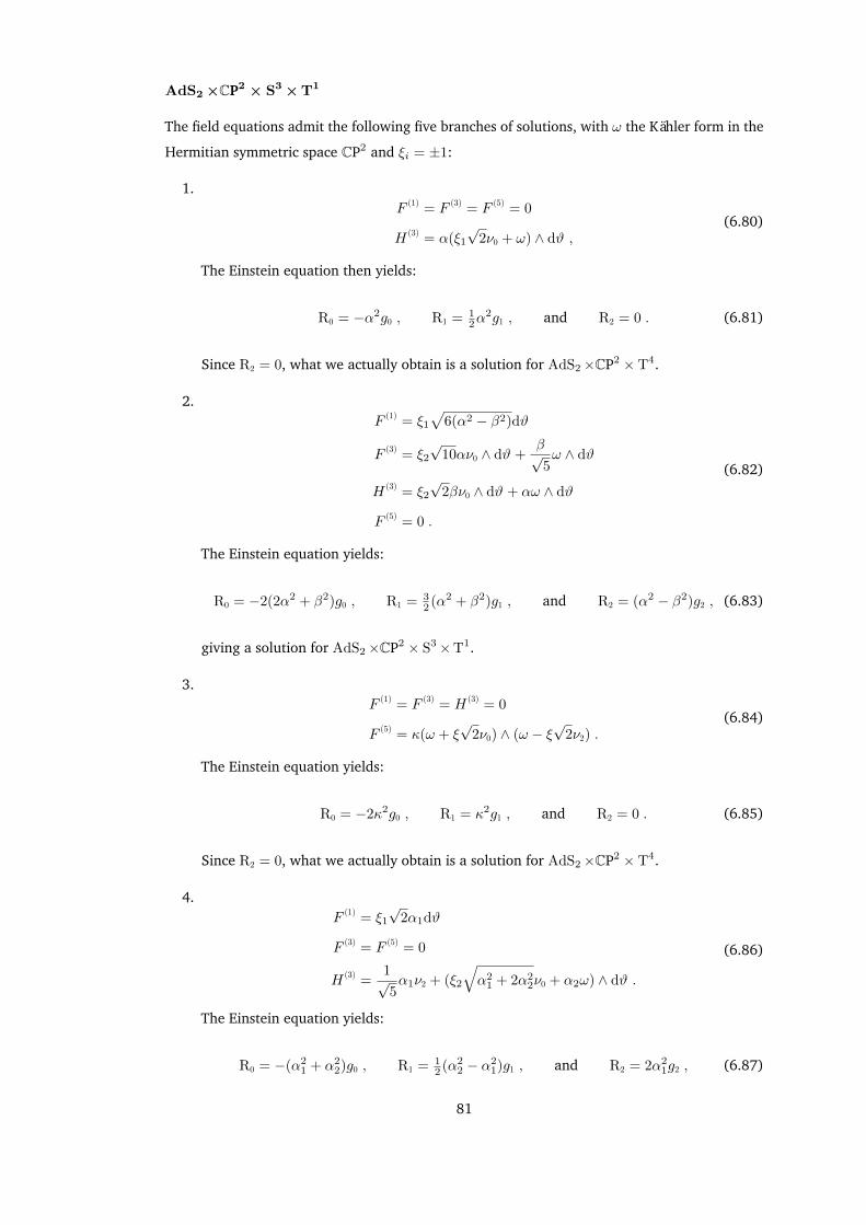
AdS2×CP2 × S3×T1
The field equations admit the following five branches of solutions, with ω the Kähler form in the
Hermitian symmetric space CP2 and ξi = ±1:
1.F (1) = F (3) = F (5) = 0
H (3) = α(ξ1√
2ν0 + ω) ∧ dϑ ,(6.80)
The Einstein equation then yields:
R0 = −α2g0 , R1 = 12α
2g1 , and R2 = 0 . (6.81)
Since R2 = 0, what we actually obtain is a solution for AdS2×CP2 × T4.
2.F (1) = ξ1
√6(α2 − β2)dϑ
F (3) = ξ2√
10αν0 ∧ dϑ +β√5ω ∧ dϑ
H (3) = ξ2√
2βν0 ∧ dϑ + αω ∧ dϑ
F (5) = 0 .
(6.82)
The Einstein equation yields:
R0 = −2(2α2 + β2)g0 , R1 = 32 (α2 + β2)g1 , and R2 = (α2 − β2)g2 , (6.83)
giving a solution for AdS2×CP2 × S3×T1.
3.F (1) = F (3) = H (3) = 0
F (5) = κ(ω + ξ√
2ν0) ∧ (ω − ξ√
2ν2) .(6.84)
The Einstein equation yields:
R0 = −2κ2g0 , R1 = κ2g1 , and R2 = 0 . (6.85)
Since R2 = 0, what we actually obtain is a solution for AdS2×CP2 × T4.
4.F (1) = ξ1
√2α1dϑ
F (3) = F (5) = 0
H (3) =1√5α1ν2 + (ξ2
√α2
1 + 2α22ν0 + α2ω) ∧ dϑ .
(6.86)
The Einstein equation yields:
R0 = −(α21 + α2
2)g0 , R1 = 12 (α2
2 − α21)g1 , and R2 = 2α2
1g2 , (6.87)
81
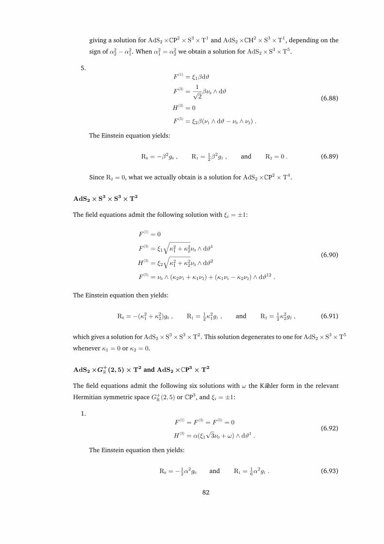
giving a solution for AdS2×CP2 × S3×T1 and AdS2×CH2 × S3×T1, depending on the
sign of α22 − α2
1. When α21 = α2
2 we obtain a solution for AdS2× S3×T5.
5.F (1) = ξ1βdϑ
F (3) =1√2βν0 ∧ dϑ
H (3) = 0
F (5) = ξ2β(ν1 ∧ dϑ − ν0 ∧ ν2) .
(6.88)
The Einstein equation yields:
R0 = −β2g0 , R1 = 12β
2g1 , and R2 = 0 . (6.89)
Since R2 = 0, what we actually obtain is a solution for AdS2×CP2 × T4.
AdS2×S3×S3×T2
The field equations admit the following solution with ξi = ±1:
F (1) = 0
F (3) = ξ1
√κ2
1 + κ22ν0 ∧ dϑ1
H (3) = ξ2
√κ2
1 + κ22ν0 ∧ dϑ2
F (5) = ν0 ∧ (κ2ν1 + κ1ν2) + (κ1ν1 − κ2ν2) ∧ dϑ12 .
(6.90)
The Einstein equation then yields:
R0 = −(κ21 + κ2
2)g0 , R1 = 12κ
21g1 , and R2 = 1
2κ22g2 , (6.91)
which gives a solution for AdS2×S3×S3×T2. This solution degenerates to one for AdS2×S3×T5
whenever κ1 = 0 or κ2 = 0.
AdS2×G+R (2, 5)× T2 and AdS2×CP3 × T2
The field equations admit the following six solutions with ω the Kähler form in the relevant
Hermitian symmetric space G+R (2, 5) or CP3, and ξi = ±1:
1.F (1) = F (3) = F (5) = 0
H (3) = α(ξ1√
3ν0 + ω) ∧ dϑ1 .(6.92)
The Einstein equation then yields:
R0 = − 12α
2g0 and R1 = 16α
2g1 . (6.93)
82
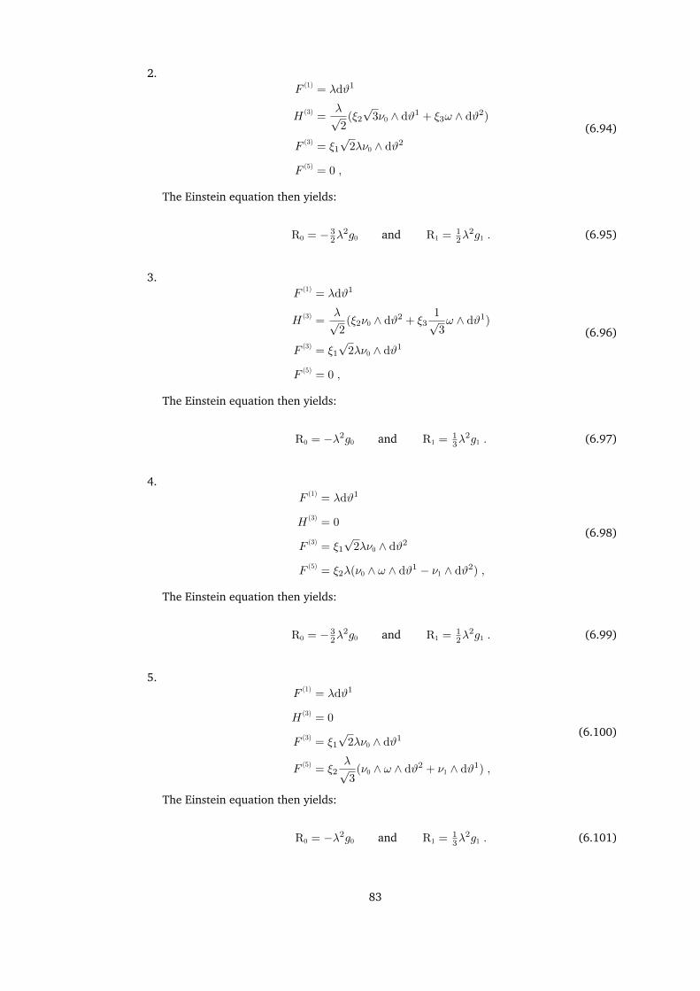
2.F (1) = λdϑ1
H (3) =λ√2
(ξ2√
3ν0 ∧ dϑ1 + ξ3ω ∧ dϑ2)
F (3) = ξ1√
2λν0 ∧ dϑ2
F (5) = 0 ,
(6.94)
The Einstein equation then yields:
R0 = − 32λ
2g0 and R1 = 12λ
2g1 . (6.95)
3.F (1) = λdϑ1
H (3) =λ√2
(ξ2ν0 ∧ dϑ2 + ξ31√3ω ∧ dϑ1)
F (3) = ξ1√
2λν0 ∧ dϑ1
F (5) = 0 ,
(6.96)
The Einstein equation then yields:
R0 = −λ2g0 and R1 = 13λ
2g1 . (6.97)
4.F (1) = λdϑ1
H (3) = 0
F (3) = ξ1√
2λν0 ∧ dϑ2
F (5) = ξ2λ(ν0 ∧ ω ∧ dϑ1 − ν1 ∧ dϑ2) ,
(6.98)
The Einstein equation then yields:
R0 = − 32λ
2g0 and R1 = 12λ
2g1 . (6.99)
5.F (1) = λdϑ1
H (3) = 0
F (3) = ξ1√
2λν0 ∧ dϑ1
F (5) = ξ2λ√3
(ν0 ∧ ω ∧ dϑ2 + ν1 ∧ dϑ1) ,
(6.100)
The Einstein equation then yields:
R0 = −λ2g0 and R1 = 13λ
2g1 . (6.101)
83
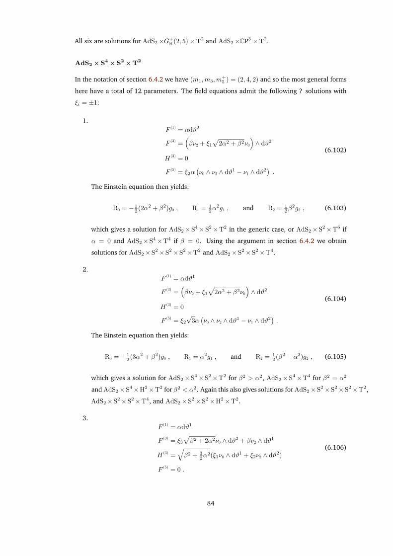
All six are solutions for AdS2×G+R (2, 5)× T2 and AdS2×CP3 × T2.
AdS2×S4×S2×T2
In the notation of section 6.4.2 we have (m1,m3,m+5 ) = (2, 4, 2) and so the most general forms
here have a total of 12 parameters. The field equations admit the following ? solutions with
ξi = ±1:
1.F (1) = αdϑ2
F (3) =(βν2 + ξ1
√2α2 + β2ν0
)∧ dϑ2
H (3) = 0
F (5) = ξ2α(ν0 ∧ ν2 ∧ dϑ1 − ν1 ∧ dϑ2
).
(6.102)
The Einstein equation then yields:
R0 = − 12 (2α2 + β2)g0 , R1 = 1
2α2g1 , and R2 = 1
2β2g2 , (6.103)
which gives a solution for AdS2×S4×S2×T2 in the generic case, or AdS2×S2×T6 if
α = 0 and AdS2×S4×T4 if β = 0. Using the argument in section 6.4.2 we obtain
solutions for AdS2× S2×S2×S2×T2 and AdS2×S2× S2×T4.
2.F (1) = αdϑ1
F (3) =(βν2 + ξ1
√2α2 + β2ν0
)∧ dϑ2
H (3) = 0
F (5) = ξ2√
3α(ν0 ∧ ν2 ∧ dϑ1 − ν1 ∧ dϑ2
).
(6.104)
The Einstein equation then yields:
R0 = − 12 (3α2 + β2)g0 , R1 = α2g1 , and R2 = 1
2 (β2 − α2)g2 , (6.105)
which gives a solution for AdS2×S4×S2×T2 for β2 > α2, AdS2× S4×T4 for β2 = α2
and AdS2×S4×H2×T2 for β2 < α2. Again this also gives solutions for AdS2×S2×S2×S2×T2,
AdS2× S2×S2×T4, and AdS2×S2×S2×H2×T2.
3.F (1) = αdϑ1
F (3) = ξ3√β2 + 2α2ν0 ∧ dϑ2 + βν2 ∧ dϑ1
H (3) =√β2 + 3
2α2(ξ1ν0 ∧ dϑ1 + ξ2ν2 ∧ dϑ2)
F (5) = 0 .
(6.106)
84
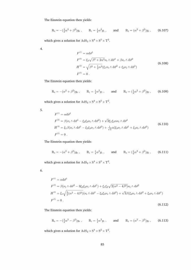
The Einstein equation then yields:
R0 = −( 32α
2 + β2)g0 , R1 = 14α
2g1 , and R2 = (α2 + β2)g2 , (6.107)
which gives a solution for AdS2×S4×S2×T2.
4.F (1) = αdϑ1
F (3) = ξ3√β2 + 2α2ν0 ∧ dϑ1 + βν2 ∧ dϑ2
H (3) =√β2 + 1
2α2(ξ1ν0 ∧ dϑ2 + ξ2ν2 ∧ dϑ1)
F (5) = 0 .
(6.108)
The Einstein equation then yields:
R0 = −(α2 + β2)g0 , R1 = 14α
2g1 , and R2 = ( 12α
2 + β2)g2 , (6.109)
which gives a solution for AdS2×S4×S2×T2.
5.F (1) = αdϑ1
F (3) = β(ν2 ∧ dϑ1 − ξ2ξ3ν0 ∧ dϑ2) +√
2ξ1ξ3αν0 ∧ dϑ1
H (3) = ξ1β(ν0 ∧ dϑ1 − ξ2ξ3ν2 ∧ dϑ2) + 1√2α(ξ3ν2 ∧ dϑ1 + ξ2ν0 ∧ dϑ2)
F (5) = 0 .
(6.110)
The Einstein equation then yields:
R0 = −(α2 + β2)g0 , R1 = 14α
2g1 , and R2 = ( 12α
2 + β2)g2 , (6.111)
which gives a solution for AdS2×S4×S2×T2.
6.
F (1) = αdϑ1
F (3) = β(ν2 ∧ dϑ2 − 3ξ2ξ3ν0 ∧ dϑ1) + ξ1ξ3√
2(α2 − 4β2)ν0 ∧ dϑ2
H (3) = ξ1
√32 (α2 − 4β2)(ν0 ∧ dϑ1 − ξ2ξ3ν2 ∧ dϑ2) +
√3β(ξ2ν0 ∧ dϑ2 + ξ3ν2 ∧ dϑ1)
F (5) = 0 .
(6.112)
The Einstein equation then yields:
R0 = −( 32α
2 − β2)g0 , R1 = 14α
2g1 , and R2 = (α2 − β2)g2 , (6.113)
which gives a solution for AdS2×S4×S2×T2.
85
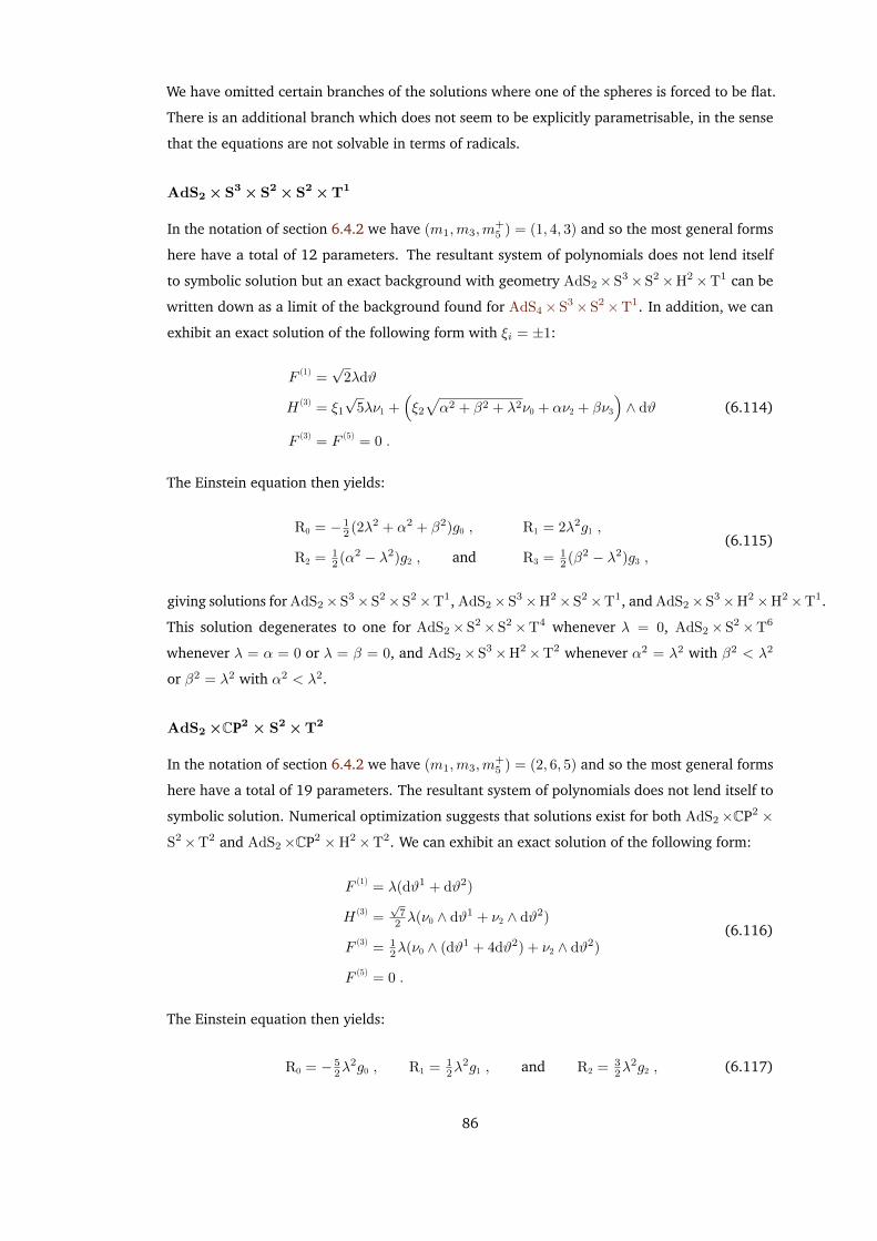
We have omitted certain branches of the solutions where one of the spheres is forced to be flat.
There is an additional branch which does not seem to be explicitly parametrisable, in the sense
that the equations are not solvable in terms of radicals.
AdS2×S3×S2× S2×T1
In the notation of section 6.4.2 we have (m1,m3,m+5 ) = (1, 4, 3) and so the most general forms
here have a total of 12 parameters. The resultant system of polynomials does not lend itself
to symbolic solution but an exact background with geometry AdS2×S3×S2×H2×T1 can be
written down as a limit of the background found for AdS4×S3×S2×T1. In addition, we can
exhibit an exact solution of the following form with ξi = ±1:
F (1) =√
2λdϑ
H (3) = ξ1√
5λν1 +(ξ2√α2 + β2 + λ2ν0 + αν2 + βν3
)∧ dϑ
F (3) = F (5) = 0 .
(6.114)
The Einstein equation then yields:
R0 = − 12 (2λ2 + α2 + β2)g0 , R1 = 2λ2g1 ,
R2 = 12 (α2 − λ2)g2 , and R3 = 1
2 (β2 − λ2)g3 ,(6.115)
giving solutions for AdS2×S3×S2×S2×T1, AdS2×S3×H2× S2×T1, and AdS2×S3×H2×H2×T1.
This solution degenerates to one for AdS2×S2×S2×T4 whenever λ = 0, AdS2×S2×T6
whenever λ = α = 0 or λ = β = 0, and AdS2×S3×H2×T2 whenever α2 = λ2 with β2 < λ2
or β2 = λ2 with α2 < λ2.
AdS2×CP2 × S2×T2
In the notation of section 6.4.2 we have (m1,m3,m+5 ) = (2, 6, 5) and so the most general forms
here have a total of 19 parameters. The resultant system of polynomials does not lend itself to
symbolic solution. Numerical optimization suggests that solutions exist for both AdS2×CP2 ×
S2×T2 and AdS2×CP2 ×H2×T2. We can exhibit an exact solution of the following form:
F (1) = λ(dϑ1 + dϑ2)
H (3) =√
72 λ(ν0 ∧ dϑ1 + ν2 ∧ dϑ2)
F (3) = 12λ(ν0 ∧ (dϑ1 + 4dϑ2) + ν2 ∧ dϑ2)
F (5) = 0 .
(6.116)
The Einstein equation then yields:
R0 = − 52λ
2g0 , R1 = 12λ
2g1 , and R2 = 32λ
2g2 , (6.117)
86
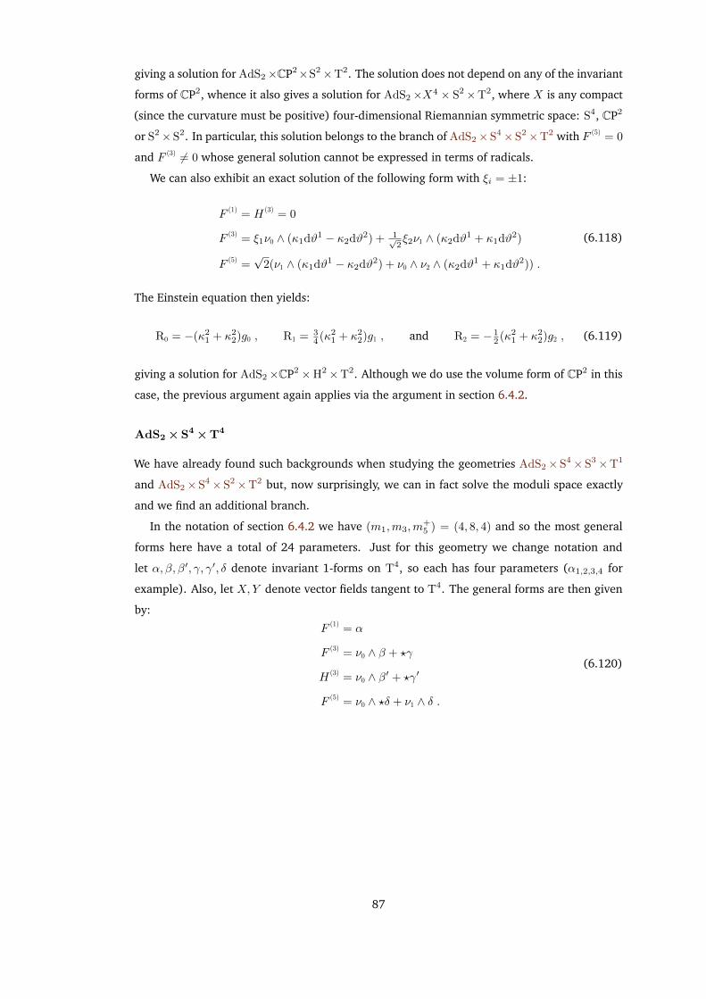
giving a solution for AdS2×CP2×S2×T2. The solution does not depend on any of the invariant
forms of CP2, whence it also gives a solution for AdS2×X4 × S2×T2, where X is any compact
(since the curvature must be positive) four-dimensional Riemannian symmetric space: S4, CP2
or S2× S2. In particular, this solution belongs to the branch of AdS2×S4×S2×T2 with F (5) = 0
and F (3) 6= 0 whose general solution cannot be expressed in terms of radicals.
We can also exhibit an exact solution of the following form with ξi = ±1:
F (1) = H (3) = 0
F (3) = ξ1ν0 ∧ (κ1dϑ1 − κ2dϑ2) + 1√2ξ2ν1 ∧ (κ2dϑ1 + κ1dϑ2)
F (5) =√
2(ν1 ∧ (κ1dϑ1 − κ2dϑ2) + ν0 ∧ ν2 ∧ (κ2dϑ1 + κ1dϑ2)) .
(6.118)
The Einstein equation then yields:
R0 = −(κ21 + κ2
2)g0 , R1 = 34 (κ2
1 + κ22)g1 , and R2 = − 1
2 (κ21 + κ2
2)g2 , (6.119)
giving a solution for AdS2×CP2 ×H2×T2. Although we do use the volume form of CP2 in this
case, the previous argument again applies via the argument in section 6.4.2.
AdS2×S4×T4
We have already found such backgrounds when studying the geometries AdS2×S4×S3×T1
and AdS2×S4×S2×T2 but, now surprisingly, we can in fact solve the moduli space exactly
and we find an additional branch.
In the notation of section 6.4.2 we have (m1,m3,m+5 ) = (4, 8, 4) and so the most general
forms here have a total of 24 parameters. Just for this geometry we change notation and
let α, β, β′, γ, γ′, δ denote invariant 1-forms on T4, so each has four parameters (α1,2,3,4 for
example). Also, let X,Y denote vector fields tangent to T4. The general forms are then given
by:
F (1) = α
F (3) = ν0 ∧ β + ?γ
H (3) = ν0 ∧ β′ + ?γ′
F (5) = ν0 ∧ ?δ + ν1 ∧ δ .
(6.120)
87
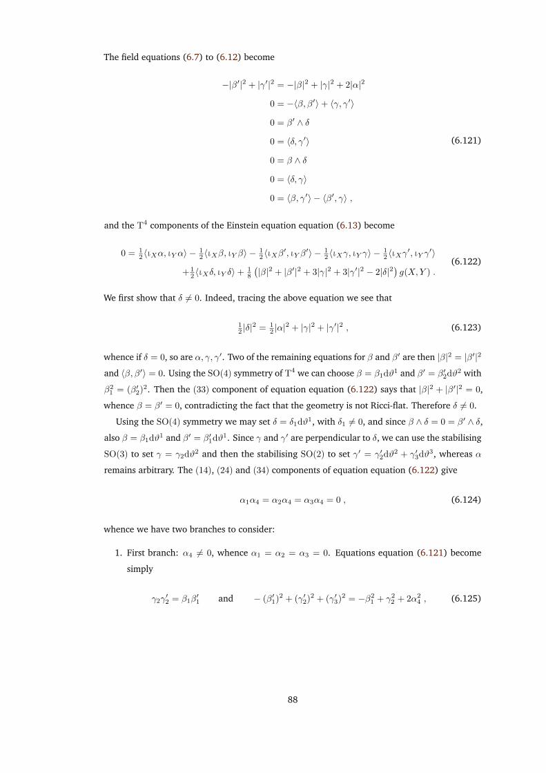
The field equations (6.7) to (6.12) become
−|β′|2 + |γ′|2 = −|β|2 + |γ|2 + 2|α|2
0 = −〈β, β′〉+ 〈γ, γ′〉
0 = β′ ∧ δ
0 = 〈δ, γ′〉
0 = β ∧ δ
0 = 〈δ, γ〉
0 = 〈β, γ′〉 − 〈β′, γ〉 ,
(6.121)
and the T4 components of the Einstein equation equation (6.13) become
0 = 12 〈ιXα, ιY α〉 −
12 〈ιXβ, ιY β〉 −
12 〈ιXβ
′, ιY β′〉 − 1
2 〈ιXγ, ιY γ〉 −12 〈ιXγ
′, ιY γ′〉
+ 12 〈ιXδ, ιY δ〉+ 1
8
(|β|2 + |β′|2 + 3|γ|2 + 3|γ′|2 − 2|δ|2
)g(X,Y ) .
(6.122)
We first show that δ 6= 0. Indeed, tracing the above equation we see that
12 |δ|
2 = 12 |α|
2 + |γ|2 + |γ′|2 , (6.123)
whence if δ = 0, so are α, γ, γ′. Two of the remaining equations for β and β′ are then |β|2 = |β′|2
and 〈β, β′〉 = 0. Using the SO(4) symmetry of T4 we can choose β = β1dϑ1 and β′ = β′2dϑ2 with
β21 = (β′2)2. Then the (33) component of equation equation (6.122) says that |β|2 + |β′|2 = 0,
whence β = β′ = 0, contradicting the fact that the geometry is not Ricci-flat. Therefore δ 6= 0.
Using the SO(4) symmetry we may set δ = δ1dϑ1, with δ1 6= 0, and since β ∧ δ = 0 = β′ ∧ δ,
also β = β1dϑ1 and β′ = β′1dϑ1. Since γ and γ′ are perpendicular to δ, we can use the stabilising
SO(3) to set γ = γ2dϑ2 and then the stabilising SO(2) to set γ′ = γ′2dϑ2 + γ′3dϑ3, whereas α
remains arbitrary. The (14), (24) and (34) components of equation equation (6.122) give
α1α4 = α2α4 = α3α4 = 0 , (6.124)
whence we have two branches to consider:
1. First branch: α4 6= 0, whence α1 = α2 = α3 = 0. Equations equation (6.121) become
simply
γ2γ′2 = β1β
′1 and − (β′1)2 + (γ′2)2 + (γ′3)2 = −β2
1 + γ22 + 2α2
4 , (6.125)
88
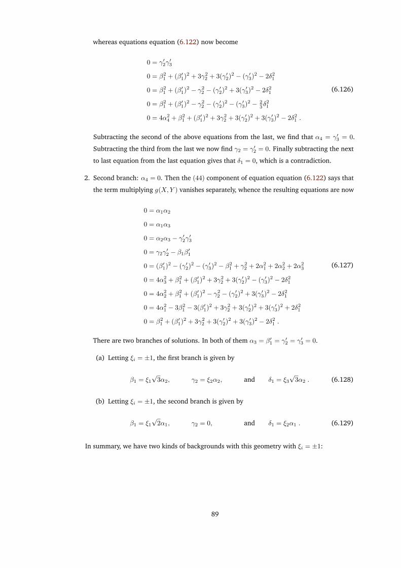
whereas equations equation (6.122) now become
0 = γ′2γ′3
0 = β21 + (β′1)2 + 3γ2
2 + 3(γ′2)2 − (γ′3)2 − 2δ21
0 = β21 + (β′1)2 − γ2
2 − (γ′2)2 + 3(γ′3)2 − 2δ21
0 = β21 + (β′1)2 − γ2
2 − (γ′2)2 − (γ′3)2 − 23δ
21
0 = 4α24 + β2
1 + (β′1)2 + 3γ22 + 3(γ′2)2 + 3(γ′3)2 − 2δ2
1 .
(6.126)
Subtracting the second of the above equations from the last, we find that α4 = γ′3 = 0.
Subtracting the third from the last we now find γ2 = γ′2 = 0. Finally subtracting the next
to last equation from the last equation gives that δ1 = 0, which is a contradiction.
2. Second branch: α4 = 0. Then the (44) component of equation equation (6.122) says that
the term multiplying g(X,Y ) vanishes separately, whence the resulting equations are now
0 = α1α2
0 = α1α3
0 = α2α3 − γ′2γ′3
0 = γ2γ′2 − β1β
′1
0 = (β′1)2 − (γ′2)2 − (γ′3)2 − β21 + γ2
2 + 2α21 + 2α2
2 + 2α23
0 = 4α23 + β2
1 + (β′1)2 + 3γ22 + 3(γ′2)2 − (γ′3)2 − 2δ2
1
0 = 4α22 + β2
1 + (β′1)2 − γ22 − (γ′2)2 + 3(γ′3)2 − 2δ2
1
0 = 4α21 − 3β2
1 − 3(β′1)2 + 3γ22 + 3(γ′2)2 + 3(γ′3)2 + 2δ2
1
0 = β21 + (β′1)2 + 3γ2
2 + 3(γ′2)2 + 3(γ′3)2 − 2δ21 .
(6.127)
There are two branches of solutions. In both of them α3 = β′1 = γ′2 = γ′3 = 0.
(a) Letting ξi = ±1, the first branch is given by
β1 = ξ1√
3α2, γ2 = ξ2α2, and δ1 = ξ3√
3α2 . (6.128)
(b) Letting ξi = ±1, the second branch is given by
β1 = ξ1√
2α1, γ2 = 0, and δ1 = ξ2α1 . (6.129)
In summary, we have two kinds of backgrounds with this geometry with ξi = ±1:
89
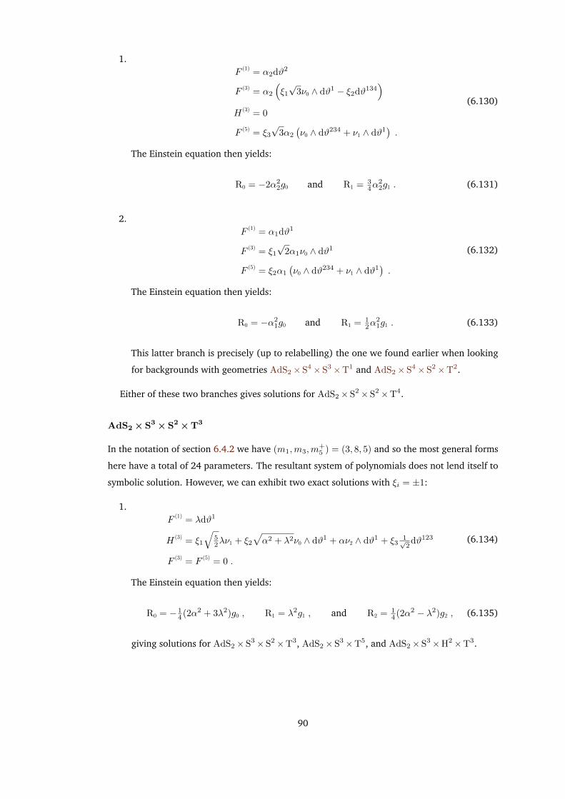
1.F (1) = α2dϑ2
F (3) = α2
(ξ1√
3ν0 ∧ dϑ1 − ξ2dϑ134)
H (3) = 0
F (5) = ξ3√
3α2
(ν0 ∧ dϑ234 + ν1 ∧ dϑ1
).
(6.130)
The Einstein equation then yields:
R0 = −2α22g0 and R1 = 3
4α22g1 . (6.131)
2.F (1) = α1dϑ1
F (3) = ξ1√
2α1ν0 ∧ dϑ1
F (5) = ξ2α1
(ν0 ∧ dϑ234 + ν1 ∧ dϑ1
).
(6.132)
The Einstein equation then yields:
R0 = −α21g0 and R1 = 1
2α21g1 . (6.133)
This latter branch is precisely (up to relabelling) the one we found earlier when looking
for backgrounds with geometries AdS2×S4×S3×T1 and AdS2×S4×S2×T2.
Either of these two branches gives solutions for AdS2×S2×S2×T4.
AdS2×S3×S2×T3
In the notation of section 6.4.2 we have (m1,m3,m+5 ) = (3, 8, 5) and so the most general forms
here have a total of 24 parameters. The resultant system of polynomials does not lend itself to
symbolic solution. However, we can exhibit two exact solutions with ξi = ±1:
1.F (1) = λdϑ1
H (3) = ξ1
√52λν1 + ξ2
√α2 + λ2ν0 ∧ dϑ1 + αν2 ∧ dϑ1 + ξ3
1√2dϑ123
F (3) = F (5) = 0 .
(6.134)
The Einstein equation then yields:
R0 = − 14 (2α2 + 3λ2)g0 , R1 = λ2g1 , and R2 = 1
4 (2α2 − λ2)g2 , (6.135)
giving solutions for AdS2×S3×S2×T3, AdS2×S3×T5, and AdS2×S3×H2×T3.
90
2. And the rather uglier,
F (1) = λdϑ3
H (3) = ξ1
√43−
√57
28λν1 + ξ2
√9 + 5
√57
56λν0 ∧ dϑ3 + ξ3
4√
3
3 +√
57λν2 ∧ dϑ3
− ξ1ξ2ξ3
√√57− 3
4
F (3) = 0
F (5) = ξ4
√2(6 +
√57)
7λ(ν1 ∧ dϑ12 + ν0 ∧ ν2 ∧ dϑ3) + ξ1ξ2ξ4
1√2λ(ν0 ∧ dϑ123 + ν1 ∧ ν2)
+ ξ1ξ3ξ4√
2λ(ν0 ∧ ν1 − ν2 ∧ dϑ123) .
(6.136)
The Einstein equation then yields:
R0 = −29 +√
57
16λ2g0 , R1 = λ2g1 , and R2 =
13 +√
57
16λ2g2 , (6.137)
giving a solution for AdS2×S3×S2×T3.
AdS2×S2×S2× S2×T2
In the notation of section 6.4.2 we have (m1,m3,m+5 ) = (2, 8, 6) and so the most general forms
here have a total of 24 parameters. The resultant system of polynomials does not lend itself
to symbolic solution. However, we know that solutions exist for AdS2×S2×S2×S2×T2 and
AdS2×S2×S2×H2×T2 as limits of the solutions for AdS2×S4×S2×T2 and AdS2×S4×H2×T2.
AdS2×CP2 × T4
In the notation of section 6.4.2 we have (m1,m3,m+5 ) = (4, 12, 10) and so the most general forms
here have a total of 38 parameters. The resultant system of polynomials does not lend itself to
symbolic solution. However, we know that solutions exist as a limit of AdS2×CP2 × S3×T1.
AdS2×S3×T5
In the notation of section 6.4.2 we have (m1,m3,m+5 ) = (5, 16, 11) and so the most general forms
here have a total of 48 parameters. The resultant system of polynomials does not lend itself
to symbolic solution. However, we know that solutions exist as limits of AdS2×S3×S3×T2,
AdS2×CP2 × S3×T1 and AdS2× S3×S2×T3.
AdS2×S2×S2×T4
In the notation of section 6.4.2 we have (m1,m3,m+5 ) = (4, 16, 12) and so the most general
forms here have a total of 48 parameters. The resultant system of polynomials does not lend
91

itself to symbolic solution. However, we know that solutions exist for both AdS2×S2×S2×T4
and AdS2×S2×H2×T4 as a limits of AdS2×S3×S2×S2×T1 and AdS2×S3×S2×H2×T1
respectively.
AdS2×S2×T6
In the notation of section 6.4.2 we have (m1,m3,m+5 ) = (6, 32, 26) and so the most general forms
here have a total of 96 parameters. The resultant system of polynomials does not lend itself
to symbolic solution. However, we know that solutions exist as a limits of AdS2× S5×S2×T1,
AdS2×SLAG3×S2×T1, AdS2× S4×S2×T2, and AdS2×S3×H3×S2.
6.4.10 Summary
We have identified (up to local isometry) all symmetric type IIB supergravity backgrounds; that
is, type IIB supergravity backgrounds whose underlying geometry is a symmetric space G/H and
with all field content G-invariant up to gauge transformations. For approximately two thirds of
all these backgrounds we have determined the full moduli space and for the rest we have shown
existence either as limits of other geometries or as exact solutions.
There are two classes of solutions, with underlying geometry either:
• Cahen-Wallach spaces (possible degenerate): CWd(λ)× R10−d, or
• Backgrounds with an Anti-de Sitter factor: AdSd×M10−d with 2 ≤ d ≤ 5 .
The Anti-de Sitter class we summarise in tables 6.2 and 6.3, distinguished by whether or not we
have determined the exact moduli space. In table 6.2 we list the backgrounds for which we have
determined the exact moduli space. There are three numbers associated to each background
that correspond to the three types of moduli:
• Geometric:
These moduli correspond to the number of free parameters of a background. One of
these moduli always corresponds to the homothety symmetry (see section 6.2.2) of the
background and so this is always ≥ 1.
• Duality:
These moduli correspond to the SL(2,R) orbit of a background (see section 6.2.2) and
can be one4 of:
0: this corresponds to backgrounds where F (1) 6= 0 ,
2: this corresponds to backgrounds where F (1) = H (3) = F (3) = 0, so that the SL(2,R)
orbit is parametrised by the axi-dilaton τ , and
3: this corresponds to backgrounds where F (1) = 0 but H (3) or F (3) are non-zero.4Geometries with multiple solution branches may have different duality moduli for each branch. The only examples
are: AdS2 ×G+R (2, 5)× T2 and AdS2 ×CP3 × T2 .
92
• Other:
These moduli correspond to the the dimension of an orbit of the action of SO(n) on back-
grounds with a Tn factor. The only non-zero example of this where we have determined
the full moduli space is AdS3×S3×T4 where, when γ 6= 0, the moduli parametrises the
orbit of SO(4) acting on the flat component of F (5) that is an (anti-)self-dual 2-form which
in R4.
In table 6.3 we list the backgrounds for which we have not determined the full moduli space.
Each background is either of the first status or one or more of the latter two:
• Some exact solutions:
We have not determined the full moduli space of the background, but have demonstrated
some exact solutions in order to show existence. There may be no other solutions, but we
cannot claim to know.
• ∃ as limit of :
The background was found as a limit of one or more other backgrounds when the radius
of curvature of one of their Riemannian factors goes to infinity (see section 6.4.2). We
thus have a family of solutions from the limit(s) but they may describe only a portion of
the full moduli space.
• ∃ from:
This can mean either:
1. The background was found by looking at a geometry with fewer flat directions, but
where the field equations forced one or more of the Riemannian factors to be flat. We
thus have a family of solutions from the limit(s) but they may describe only a portion
of the full moduli space.
2. The background can be shown to exist via the argument in section 6.4.2. We thus
have a family of solutions but they may describe only a portion of the full moduli
space.
The list of backgrounds is not particularly surprising, with only a few backgrounds that
are not AdS-sphere-flat products. We note here that symmetric supergravity backgrounds do
not necessarily oxidise to symmetric supergravity backgrounds; although the curvature of the
oxidation connection may be invariant, the oxidation connection itself may well not be invariant.
It is left to determine which of these backgrounds is supersymmetric. The spirit of this is
address in chapter 7 although we actually determine supersymmetry for symmetric M-theory
backgrounds. The same technique can be applied for symmetric type IIB backgrounds although
the dilaton component of the Killing spinor equations makes things slightly more difficult.
After the proof of Patrick Meessen’s homogeneity conjecture [34, 1, 2, 84] we were reminded
of his follow-up conjecture that all supergravity backgrounds preserving more than 3/4 of the
maximum supersymmetry are not only homogeneous but moreover symmetric. As far as we
93
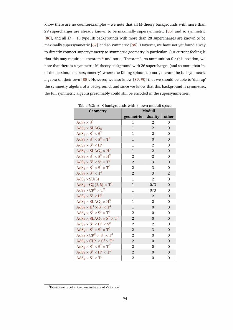
know there are no counterexamples – we note that all M-theory backgrounds with more than
29 supercharges are already known to be maximally supersymmetric [85] and so symmetric
[86], and all D = 10 type IIB backgrounds with more than 28 supercharges are known to be
maximally supersymmetric [87] and so symmetric [86]. However, we have not yet found a way
to directly connect supersymmetry to symmetric geometry in particular. Our current feeling is
that this may require a “theorem”5 and not a “Theorem”. As ammunition for this position, we
note that there is a symmetric M-theory background with 26 supercharges (and so more than 3/4
of the maximum supersymmetry) where the Killing spinors do not generate the full symmetric
algebra on their own [88]. However, we also know [89, 90] that we should be able to ‘dial up’
the symmetry algebra of a background, and since we know that this background is symmetric,
the full symmetric algebra presumably could still be encoded in the supersymmetries.
Table 6.2: AdS backgrounds with known moduli spaceGeometry Moduli
geometric duality otherAdS5×S5 1 2 0AdS5×SLAG3 1 2 0AdS5×S3×S2 1 2 0AdS4×S3×S2×T1 1 0 0AdS3×S5×H2 1 2 0AdS3×SLAG3×H2 1 2 0AdS3×S3×S2×H2 2 2 0AdS3×S3×S3×T1 2 3 0AdS3×S3×S2×T2 2 3 0AdS3×S3×T4 2 3 2AdS2×SU(3) 1 2 0AdS2×G+
R (2, 5)× T2 1 0/3 0AdS2×CP3 × T2 1 0/3 0AdS2×S5×H3 1 2 0AdS2×SLAG3×H3 1 2 0AdS2×H4×S3×T1 1 0 0AdS2×S5×S2×T1 2 0 0AdS2×SLAG3×S2×T1 2 0 0AdS2×S3×H3× S2 2 2 0AdS2×S3×S3×T2 2 3 0AdS2×CP2 × S3×T1 2 0 0AdS2×CH2 × S3×T1 2 0 0AdS2×S4×S2×T2 2 0 0AdS2×S4×H2×T2 2 0 0AdS2×S4×T4 2 0 0
5Exhaustive proof in the nomenclature of Victor Kac.
94
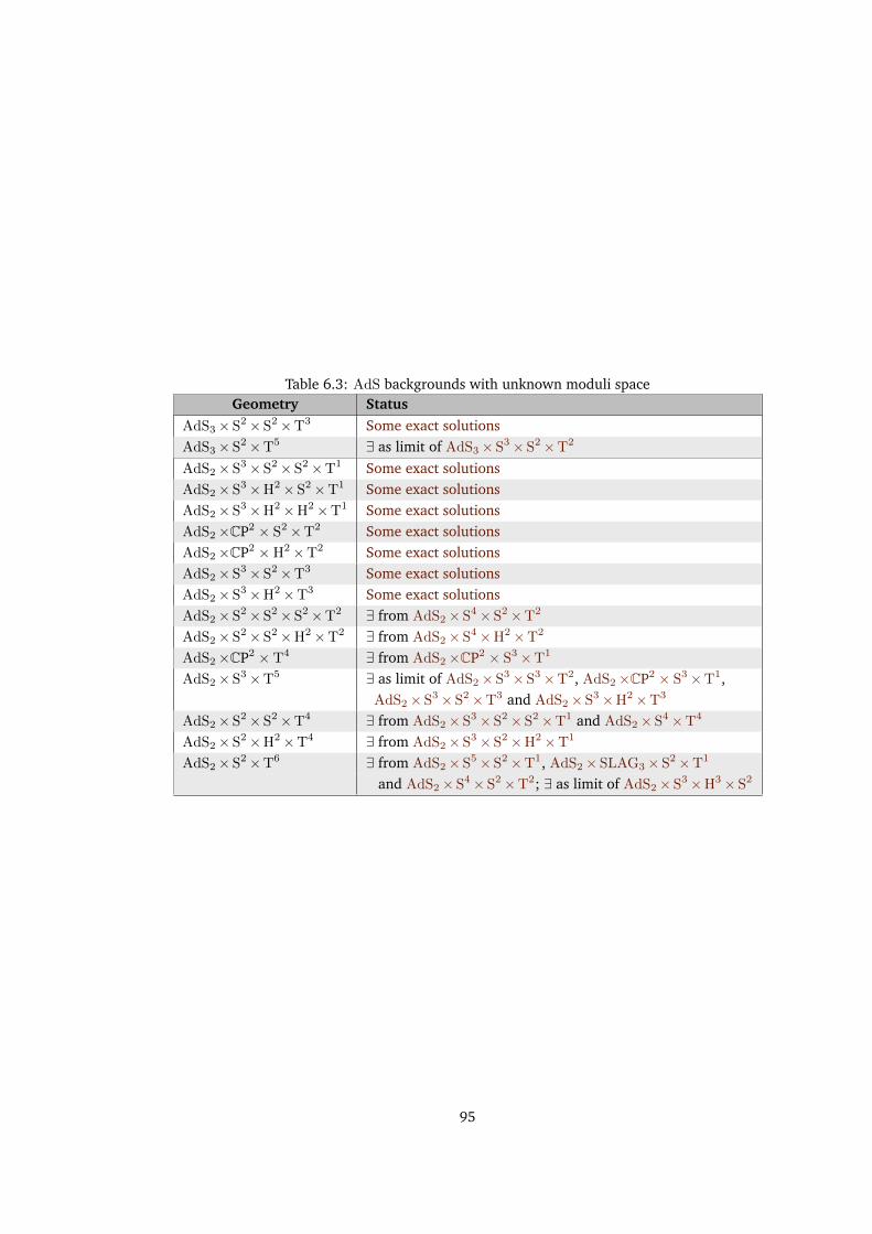
Table 6.3: AdS backgrounds with unknown moduli spaceGeometry Status
AdS3×S2×S2×T3 Some exact solutionsAdS3×S2×T5 ∃ as limit of AdS3×S3×S2×T2
AdS2×S3×S2×S2×T1 Some exact solutionsAdS2×S3×H2× S2×T1 Some exact solutionsAdS2×S3×H2×H2×T1 Some exact solutionsAdS2×CP2 × S2×T2 Some exact solutionsAdS2×CP2 ×H2×T2 Some exact solutionsAdS2×S3×S2×T3 Some exact solutionsAdS2×S3×H2×T3 Some exact solutionsAdS2×S2×S2×S2×T2 ∃ from AdS2×S4×S2×T2
AdS2×S2×S2×H2×T2 ∃ from AdS2×S4×H2×T2
AdS2×CP2 × T4 ∃ from AdS2×CP2 × S3×T1
AdS2×S3×T5 ∃ as limit of AdS2×S3×S3×T2, AdS2×CP2 × S3×T1,AdS2×S3×S2×T3 and AdS2×S3×H2×T3
AdS2×S2×S2×T4 ∃ from AdS2×S3×S2×S2×T1 and AdS2×S4×T4
AdS2×S2×H2×T4 ∃ from AdS2×S3×S2×H2×T1
AdS2×S2×T6 ∃ from AdS2×S5×S2×T1, AdS2×SLAG3×S2×T1
and AdS2×S4×S2×T2; ∃ as limit of AdS2×S3×H3×S2
95
Chapter 7
Supersymmetric symmetric M-theorybackgrounds
7.1 Introduction
A classification of all symmetric M-theory backgrounds was made in [33] (and additionally for
symmetric Type IIB backgrounds in [3]) using Élie Cartan’s classification of irreducible Rieman-
nian symmetric spaces (e.g. [32]) and Cahen and Wallach’s classification of indecomposable
Lorentzian symmetric spaces [30, 31]. However this classification dealt with backgrounds at the
bosonic level and said nothing about which backgrounds are supersymmetric. In this chapter
we build on this result by determining which symmetric M-theory backgrounds are supersym-
metric and if so what fraction of the maximum supersymmetry is preserved. This represents the
next step in classifying homogeneous M-theory backgrounds and concludes the classification of
supersymmetric symmetric M-theory backgrounds.
The general idea is as follows: The number of supersymmetries preserved by an M-theory
background (M, g, F ) is equal to the dimension of the kernel of the M-theory superconnection
D (see equation (4.2)). We use a general algorithm (derived in detail in [4]) for computing
algebraically and concretely the holonomy algebra of any invariant spinor connection on a
reductive homogeneous space to compute the holonomy algebra of D. We then identify the
dimension of the kernel of the algebra and thus the number of supersymmetries preserved by
the background. We apply this to all symmetric M-theory backgrounds listed in [33] and so
identify all supersymmetric symmetric M-theory backgrounds.
This chapter is based upon work done in collaboration with Andree Lischewski in [4].
7.2 Invariant spin connections on symmetric spaces
We give a very brief framing of the algorithm we will use to compute the supersymmetry of
symmetric M-theory backgrounds. Much more detail can be found in [4].
96
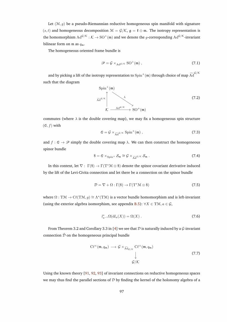
Let (M, g) be a pseudo-Riemannian reductive homogeneous spin manifold with signature
(s, t) and homogeneous decomposition M = G/K, g = k ⊕ m. The isotropy representation is
the homomorphism AdG/K : K → SO+(m) and we denote the g-corresponding AdG/K-invariant
bilinear form on m as qm.
The homogeneous oriented frame bundle is
P = G ×AdG/K SO+(m) , (7.1)
and by picking a lift of the isotropy representation to Spin+(m) through choice of map AdG/K
such that the diagram
Spin+(m)
K SO+(m)
λAdG/K
AdG/K
(7.2)
commutes (where λ is the double covering map), we may fix a homogeneous spin structure
(Q, f) with
Q = G ×AdG/K Spin+(m) , (7.3)
and f : Q → P simply the double covering map λ. We can then construct the homogeneous
spinor bundle
$ = Q ×Spin+ Sm ∼= G ×AdG/K Sm . (7.4)
In this context, let ∇ : Γ($)→ Γ(T∗M⊗ $) denote the spinor covariant derivative induced
by the lift of the Levi-Civita connection and let there be a connection on the spinor bundle
D = ∇+ Ω : Γ($)→ Γ(T∗M⊗ $) (7.5)
where Ω : TM→ C`(TM, g) ∼= Λ∗(TM) is a vector bundle homomorphism and is left-invariant
(using the exterior algebra isomorphism, see appendix B.5): ∀X ∈ TM, a ∈ G,
l∗a−1Ω(dla(X)) = Ω(X) . (7.6)
From Theorem 3.2 and Corollary 3.3 in [4] we see thatD is naturally induced by a G-invariant
connection D on the homogeneous principal bundle
C`×(m, qm) G ×AdG/K
C`×(m, qm)
G/K
(7.7)
Using the known theory [91, 92, 93] of invariant connections on reductive homogeneous spaces
we may thus find the parallel sections of D by finding the kernel of the holonomy algebra of a
97
particular map α : g→ C`(m, qm) associated to D. The map α decomposes with D = ∇+ Ω into
αk + αm of which
αk = adG/K
: k→ spin(m, qm) ⊂ C`(m, qm) , (7.8)
and
αm = Ωo : m→ C`(m, qm) . (7.9)
We also have the curvature map κ which measures the failure of α to be a Lie algebra homo-
morphism,
κ : g× g → C`(m, qm)
(X1, X2) 7→ [α(X1), α(X2)]− α([X1, X2]) ,(7.10)
Then, with Im(κ) := span(Im(κ)), hol(α) is the g-module generated by Im(κ), i.e.
hol(α) = Im(κ) + [α(g), Im(κ)] + [α(g), [α(g), Im(κ)]] + . . . ⊂ C`(m, qm) , (7.11)
and for the case of a symmetric space,
hol(α) = Im(κ) + [α(m), Im(κ)] + [α(m), [α(m), Im(κ)]] + . . . ⊂ C`(m, qm) . (7.12)
Finally, for ease of computation, we wish to work in the algebra C`(s, t) instead of C`(m, qm)
and so we fix an orientation-preserving isometry w : Rs,t → m and instead use the map αw :=
w∗α : g→ C`(s, t) (and concomitant κw : g× g→ C`(s, t)) in all calculations.
7.3 Supersymmetric symmetric M-theory backgrounds
We continue on from our earlier definition of D = 11 supergravity (see section 4.2.3). Now we
are interested in the field equations of the theory and so we begin with the action. The D = 11
(bosonic) action is (in the string frame)
S = 12
∫ (R− 1
2 |F |2)
dvol− 16F ∧ F ∧A
, (7.13)
where R is the Ricci scalar curvature of g and dvol is the signed volume element. We define the
inner product on differential forms 〈X,Y 〉dvol = X ∧ ∗Y and the norm |X|2 = 〈X,X〉.
Varying the action with respect to each of the fields yields the following (bosonic) equations
of motiond ?F = 1
2F ∧ F
Ric(X,Y ) = 12 〈ιXF, ιY F 〉 −
16g(X,Y )|F |2 .
(7.14)
In the case of a symmetric space, the 4-form F is parallel with respect to the canonical
connection (see section 2.2.1) which is the Levi-Civita connection (∇F = 0) and so its dual ?F
is also parallel (∇ ?F = 0) whence it is both closed (dF = 0) and co-closed (d ?F = 0). The
98
field equations then simplify to
0 = F ∧ F (7.15)
Ric(X,Y ) = 12 〈ιXF, ιY F 〉 −
16g(X,Y )|F |2 . (7.16)
We recall the Killing spinor equation of D = 11 supergravity (equation (4.2)) takes the form
DX = ∇X + Ω(X) where
Ω(X) = 124 (3F ·X −X · F ) . (7.17)
Killing spinors are (non-trivial) spinors parallel to this connection and the number of linearly
independent Killing spinors is equal to the number of supersymmetries of a background. It is
clear that the algorithm of section 7.2 may be applied to this connection in order to determine
the rank of the subbundle of Killing spinors and so the fraction of the maximum supersymmetry
preserved by the background.
Symmetric M-theory backgrounds have been classified in [33] and we follow that article’s
conventions (which coincide with those in section 4.2.3) and reference particular backgrounds
directly from it. Background geometries are of the form M = M0 ×M1 × . . .×Mn with M0 an
indecomposable Lorentzian symmetric space and Mi for i > 0 irreducible Riemannian symmetric
spaces, with each factor determined by its Lie algebra pair (k,m)i. From here forwards in this
chapter we will elide pullbacks and conflate F with its evaluation at the origin o.
7.4 Exclusion of backgrounds
We note that to exclude a background, it is only necessary to identify a single element in the
holonomy algebra that has trivial kernel. This element alone then ensures that the algebra has
trivial kernel. As such, we do not in general have to produce the whole holonomy algebra hol(α)
by stabilising the dimension of successive commutators of α(m) with Im(κ) in order to rule out
a background.
7.4.1 Special cases
7.4.1.1 No spin structure
We ignore all backgrounds from [33] which involve a CP2 or CH2 factor. They are solutions to
the field equations but CP2 does not admit a spin structure, and so it makes no sense to speak
about supersymmetry in this case. The non-compact dual CH2 does not admit a homogeneous
spin structure as its isotropy representation is equivalent to that of CP2.
99
7.4.1.2 n ≥ 3 and F two-factor homogeneous
Let us assume that n ≥ 3 and either:
F = F1 , or F = F1 ∧H2 ∧H3 , or F = H2 ∧H3 , (7.18)
with F1 ∈ (Λm1)k and Hi ∈ (Λhommi)k, i.e. Hi are homogeneous forms.
Now, taking X2 ∈ m2, X3 ∈ m3 such that either ιXiHi 6= 0 or ιXi
Hi = 0, we then have that
[X2, X3]k = 0 and α(Xi) ∝ Xi · F , so
κ(X2, X3) ∝ [X2 · F,X3 · F ] ∝ (X2 ·X3) · (F · F ) ∈ C`(1, 10) . (7.19)
Thus in this case F must have a kernel as considered as a spinor endomorphism or there are no
D-parallel spinors. Homogeneous elements act invertibly and so the last case is ruled out and
the first two cases are reduced to F1 having kernel. In particular, this means that F1 cannot be
homogeneous.
An immediate application of this is when n ≥ 3 and F is proportional to the volume form on
any (possibly composite) factor, then there are no D-parallel spinors.
Note that this does not apply to Freund-Rubin backgrounds because n = 2.
7.4.1.3 n ≥ 3, F two-factor homogeneous, and F1 inhomogeneous
Here we look at geometries where section 7.4.1.2 applies but the F1 factor is inhomogeneous
and so we must do a little more work.
• (4.6.1), (4.7.5): F1 = F ∝ ω ∧ ω with ω the Kähler form of a 6-dimensional factor
The action of ω on the (complex) spinor module is well known [94] and using these results
it is straightforward to see that F considered as an endomorphism on the spinor module
has no zero eigenvalue if M1 is 6-dimensional. This is easily verified with a concrete
realisation of F .
• (4.7.6): F1 ∈ (Λ4m0)k ⊕ (Λ4m1)k is decomposable and has trivial kernel on both factors;
so F1 has trivial kernel.
• (4.7.7): F1 ∈ (Λ4m1)k ⊕ (Λ4m2)k is decomposable and has trivial kernel on both factors;
so F1 has trivial kernel.
7.4.1.4 A background that isn’t a background
We suggest that the classical background (4.7.4): AdS2×GC(2, 4) × T1 does not exist. There
are two polynomial equations resulting from the field equation F ∧ F = 0, the second of which
is not found in [33]. In the notation of [33] this is f21 + f2
2 = 0 and it means that no background
with such an underlying geometry exists.
100
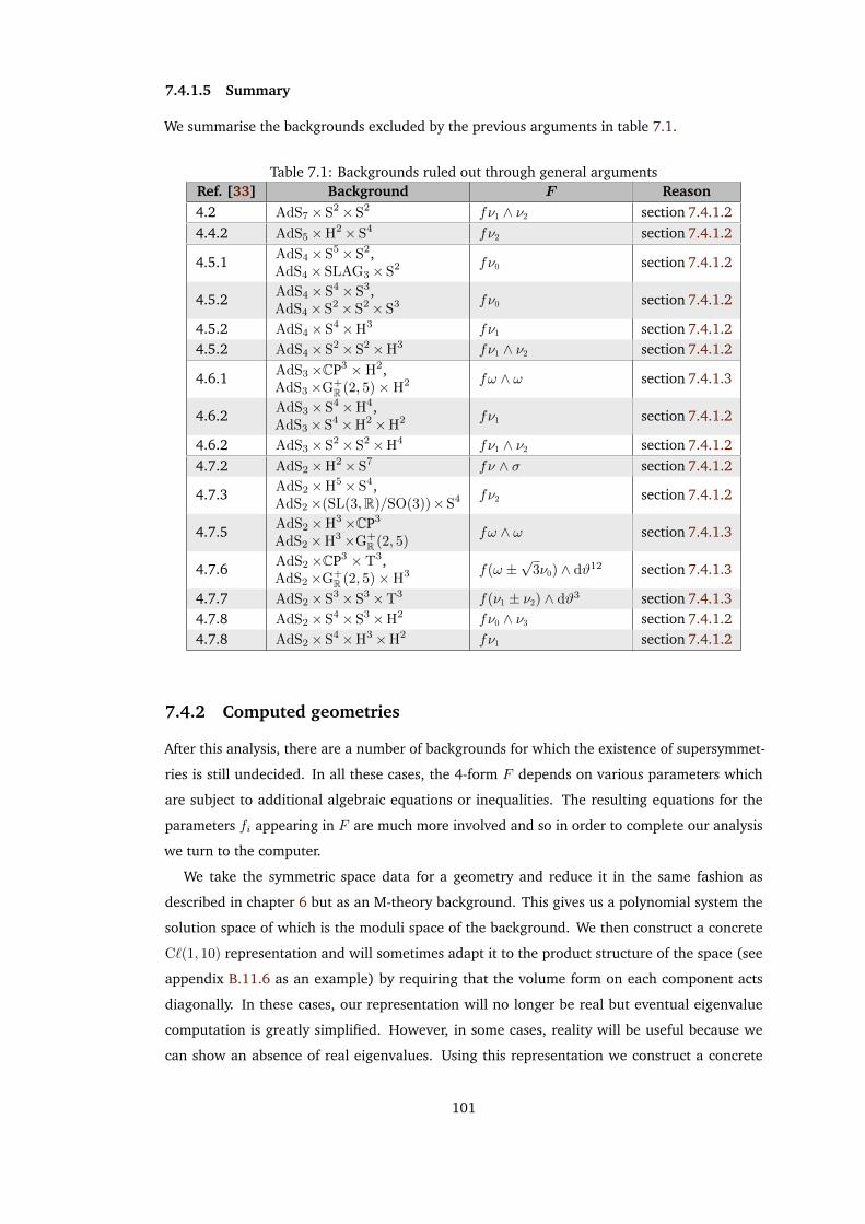
7.4.1.5 Summary
We summarise the backgrounds excluded by the previous arguments in table 7.1.
Table 7.1: Backgrounds ruled out through general argumentsRef. [33] Background F Reason4.2 AdS7×S2×S2 fν1 ∧ ν2 section 7.4.1.24.4.2 AdS5×H2×S4 fν2 section 7.4.1.2
4.5.1AdS4×S5×S2,AdS4×SLAG3×S2 fν0 section 7.4.1.2
4.5.2AdS4×S4×S3,AdS4×S2× S2×S3 fν0 section 7.4.1.2
4.5.2 AdS4×S4×H3 fν1 section 7.4.1.24.5.2 AdS4×S2×S2×H3 fν1 ∧ ν2 section 7.4.1.2
4.6.1AdS3×CP3 ×H2,AdS3×G+
R (2, 5)×H2 fω ∧ ω section 7.4.1.3
4.6.2AdS3×S4×H4,AdS3×S4×H2×H2 fν1 section 7.4.1.2
4.6.2 AdS3×S2×S2×H4 fν1 ∧ ν2 section 7.4.1.24.7.2 AdS2×H2×S7 fν ∧ σ section 7.4.1.2
4.7.3AdS2×H5×S4,AdS2×(SL(3,R)/SO(3))×S4 fν2 section 7.4.1.2
4.7.5AdS2×H3×CP3
AdS2×H3×G+R (2, 5)
fω ∧ ω section 7.4.1.3
4.7.6AdS2×CP3 × T3,AdS2×G+
R (2, 5)×H3 f(ω ±√
3ν0) ∧ dϑ12 section 7.4.1.3
4.7.7 AdS2×S3×S3×T3 f(ν1 ± ν2) ∧ dϑ3 section 7.4.1.34.7.8 AdS2×S4×S3×H2 fν0 ∧ ν3 section 7.4.1.24.7.8 AdS2×S4×H3×H2 fν1 section 7.4.1.2
7.4.2 Computed geometries
After this analysis, there are a number of backgrounds for which the existence of supersymmet-
ries is still undecided. In all these cases, the 4-form F depends on various parameters which
are subject to additional algebraic equations or inequalities. The resulting equations for the
parameters fi appearing in F are much more involved and so in order to complete our analysis
we turn to the computer.
We take the symmetric space data for a geometry and reduce it in the same fashion as
described in chapter 6 but as an M-theory background. This gives us a polynomial system the
solution space of which is the moduli space of the background. We then construct a concrete
C`(1, 10) representation and will sometimes adapt it to the product structure of the space (see
appendix B.11.6 as an example) by requiring that the volume form on each component acts
diagonally. In these cases, our representation will no longer be real but eventual eigenvalue
computation is greatly simplified. However, in some cases, reality will be useful because we
can show an absence of real eigenvalues. Using this representation we construct a concrete
101
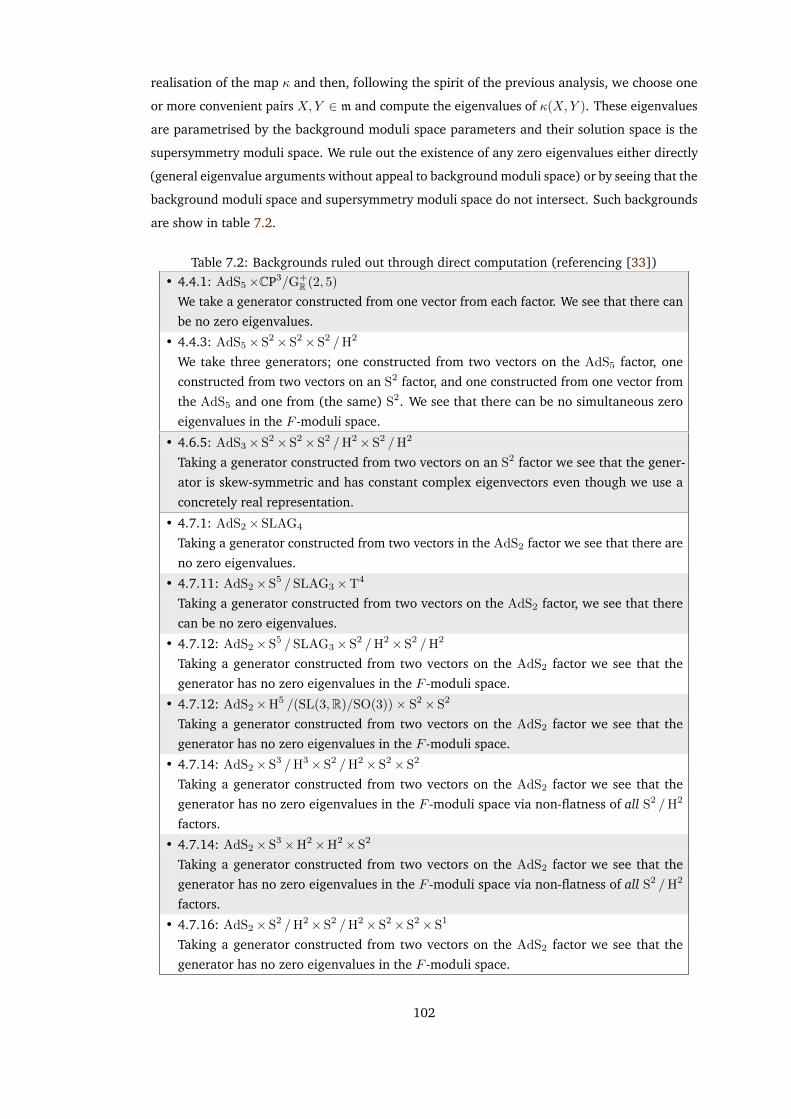
realisation of the map κ and then, following the spirit of the previous analysis, we choose one
or more convenient pairs X,Y ∈ m and compute the eigenvalues of κ(X,Y ). These eigenvalues
are parametrised by the background moduli space parameters and their solution space is the
supersymmetry moduli space. We rule out the existence of any zero eigenvalues either directly
(general eigenvalue arguments without appeal to background moduli space) or by seeing that the
background moduli space and supersymmetry moduli space do not intersect. Such backgrounds
are show in table 7.2.
Table 7.2: Backgrounds ruled out through direct computation (referencing [33])• 4.4.1: AdS5×CP3/G+
R (2, 5)
We take a generator constructed from one vector from each factor. We see that there can
be no zero eigenvalues.
• 4.4.3: AdS5×S2× S2×S2 /H2
We take three generators; one constructed from two vectors on the AdS5 factor, one
constructed from two vectors on an S2 factor, and one constructed from one vector from
the AdS5 and one from (the same) S2. We see that there can be no simultaneous zero
eigenvalues in the F -moduli space.
• 4.6.5: AdS3×S2× S2×S2 /H2× S2 /H2
Taking a generator constructed from two vectors on an S2 factor we see that the gener-
ator is skew-symmetric and has constant complex eigenvectors even though we use a
concretely real representation.
• 4.7.1: AdS2×SLAG4
Taking a generator constructed from two vectors in the AdS2 factor we see that there are
no zero eigenvalues.
• 4.7.11: AdS2×S5 /SLAG3×T4
Taking a generator constructed from two vectors on the AdS2 factor, we see that there
can be no zero eigenvalues.
• 4.7.12: AdS2×S5 /SLAG3×S2 /H2×S2 /H2
Taking a generator constructed from two vectors on the AdS2 factor we see that the
generator has no zero eigenvalues in the F -moduli space.
• 4.7.12: AdS2×H5 /(SL(3,R)/SO(3))× S2×S2
Taking a generator constructed from two vectors on the AdS2 factor we see that the
generator has no zero eigenvalues in the F -moduli space.
• 4.7.14: AdS2×S3 /H3×S2 /H2×S2×S2
Taking a generator constructed from two vectors on the AdS2 factor we see that the
generator has no zero eigenvalues in the F -moduli space via non-flatness of all S2 /H2
factors.
• 4.7.14: AdS2×S3×H2×H2×S2
Taking a generator constructed from two vectors on the AdS2 factor we see that the
generator has no zero eigenvalues in the F -moduli space via non-flatness of all S2 /H2
factors.
• 4.7.16: AdS2×S2 /H2×S2 /H2×S2×S2×S1
Taking a generator constructed from two vectors on the AdS2 factor we see that the
generator has no zero eigenvalues in the F -moduli space.
102
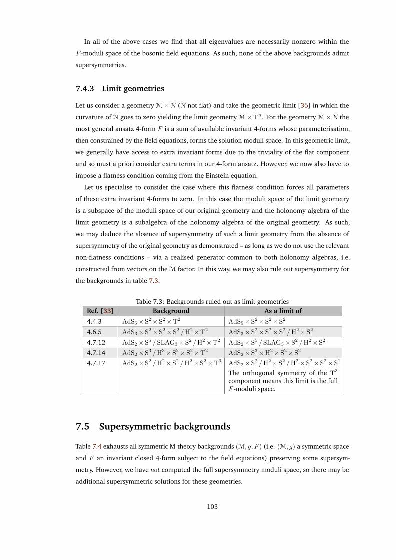
In all of the above cases we find that all eigenvalues are necessarily nonzero within the
F -moduli space of the bosonic field equations. As such, none of the above backgrounds admit
supersymmetries.
7.4.3 Limit geometries
Let us consider a geometry M×N (N not flat) and take the geometric limit [36] in which the
curvature of N goes to zero yielding the limit geometry M× Tn. For the geometry M×N the
most general ansatz 4-form F is a sum of available invariant 4-forms whose parameterisation,
then constrained by the field equations, forms the solution moduli space. In this geometric limit,
we generally have access to extra invariant forms due to the triviality of the flat component
and so must a priori consider extra terms in our 4-form ansatz. However, we now also have to
impose a flatness condition coming from the Einstein equation.
Let us specialise to consider the case where this flatness condition forces all parameters
of these extra invariant 4-forms to zero. In this case the moduli space of the limit geometry
is a subspace of the moduli space of our original geometry and the holonomy algebra of the
limit geometry is a subalgebra of the holonomy algebra of the original geometry. As such,
we may deduce the absence of supersymmetry of such a limit geometry from the absence of
supersymmetry of the original geometry as demonstrated – as long as we do not use the relevant
non-flatness conditions – via a realised generator common to both holonomy algebras, i.e.
constructed from vectors on the M factor. In this way, we may also rule out supersymmetry for
the backgrounds in table 7.3.
Table 7.3: Backgrounds ruled out as limit geometriesRef. [33] Background As a limit of
4.4.3 AdS5×S2×S2×T2 AdS5×S2×S2×S2
4.6.5 AdS3×S2×S2×S2 /H2×T2 AdS3×S2×S2×S2 /H2×S2
4.7.12 AdS2×S5 / SLAG3×S2 /H2×T2 AdS2×S5 / SLAG3×S2 /H2×S2
4.7.14 AdS2×S3 /H3×S2×S2×T2 AdS2×S3×H2×S2×S2
4.7.17 AdS2×S2 /H2×S2 /H2×S2×T3 AdS2×S2 /H2× S2 /H2×S2× S2×S1
The orthogonal symmetry of the T3
component means this limit is the fullF -moduli space.
7.5 Supersymmetric backgrounds
Table 7.4 exhausts all symmetric M-theory backgrounds (M, g, F ) (i.e. (M, g) a symmetric space
and F an invariant closed 4-form subject to the field equations) preserving some supersym-
metry. However, we have not computed the full supersymmetry moduli space, so there may be
additional supersymmetric solutions for these geometries.
103
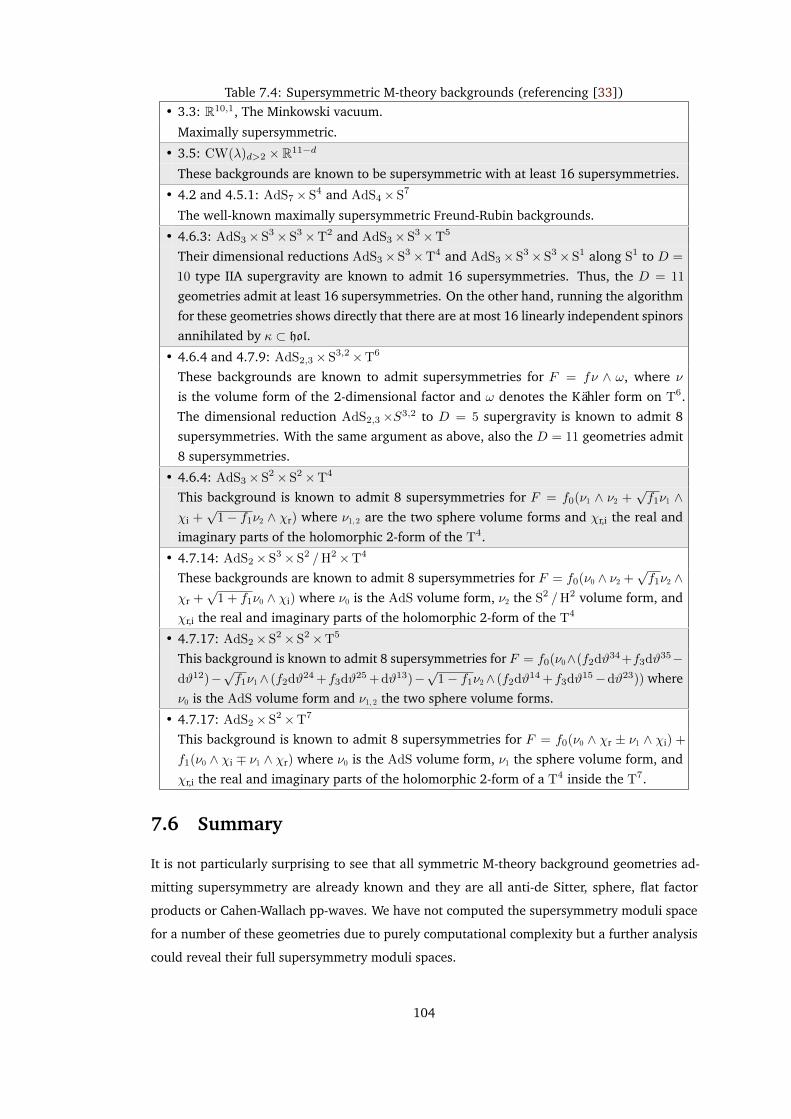
Table 7.4: Supersymmetric M-theory backgrounds (referencing [33])• 3.3: R10,1, The Minkowski vacuum.
Maximally supersymmetric.
• 3.5: CW(λ)d>2 × R11−d
These backgrounds are known to be supersymmetric with at least 16 supersymmetries.
• 4.2 and 4.5.1: AdS7×S4 and AdS4× S7
The well-known maximally supersymmetric Freund-Rubin backgrounds.
• 4.6.3: AdS3×S3× S3×T2 and AdS3×S3×T5
Their dimensional reductions AdS3× S3×T4 and AdS3×S3×S3× S1 along S1 to D =
10 type IIA supergravity are known to admit 16 supersymmetries. Thus, the D = 11
geometries admit at least 16 supersymmetries. On the other hand, running the algorithm
for these geometries shows directly that there are at most 16 linearly independent spinors
annihilated by κ ⊂ hol.
• 4.6.4 and 4.7.9: AdS2,3×S3,2×T6
These backgrounds are known to admit supersymmetries for F = fν ∧ ω, where ν
is the volume form of the 2-dimensional factor and ω denotes the Kähler form on T6.
The dimensional reduction AdS2,3×S3,2 to D = 5 supergravity is known to admit 8
supersymmetries. With the same argument as above, also the D = 11 geometries admit
8 supersymmetries.
• 4.6.4: AdS3×S2× S2×T4
This background is known to admit 8 supersymmetries for F = f0(ν1 ∧ ν2 +√f1ν1 ∧
χi +√
1− f1ν2 ∧ χr) where ν1, 2 are the two sphere volume forms and χr,i the real and
imaginary parts of the holomorphic 2-form of the T4.
• 4.7.14: AdS2×S3×S2 /H2×T4
These backgrounds are known to admit 8 supersymmetries for F = f0(ν0 ∧ ν2 +√f1ν2 ∧
χr +√
1 + f1ν0 ∧ χi) where ν0 is the AdS volume form, ν2 the S2 /H2 volume form, and
χr,i the real and imaginary parts of the holomorphic 2-form of the T4
• 4.7.17: AdS2×S2×S2×T5
This background is known to admit 8 supersymmetries for F = f0(ν0∧(f2dϑ34+f3dϑ35−dϑ12)−
√f1ν1∧ (f2dϑ24 +f3dϑ25 +dϑ13)−
√1− f1ν2∧ (f2dϑ14 +f3dϑ15−dϑ23)) where
ν0 is the AdS volume form and ν1, 2 the two sphere volume forms.
• 4.7.17: AdS2×S2×T7
This background is known to admit 8 supersymmetries for F = f0(ν0 ∧ χr ± ν1 ∧ χi) +
f1(ν0 ∧ χi ∓ ν1 ∧ χr) where ν0 is the AdS volume form, ν1 the sphere volume form, and
χr,i the real and imaginary parts of the holomorphic 2-form of a T4 inside the T7.
7.6 Summary
It is not particularly surprising to see that all symmetric M-theory background geometries ad-
mitting supersymmetry are already known and they are all anti-de Sitter, sphere, flat factor
products or Cahen-Wallach pp-waves. We have not computed the supersymmetry moduli space
for a number of these geometries due to purely computational complexity but a further analysis
could reveal their full supersymmetry moduli spaces.
104

This technique can be applied to the symmetric type IIB backgrounds of chapter 6 although
the dilaton component of the Killing spinor equations (equation (4.16)) will additionally need
to be dealt with; but this simply becomes another algebraic constraint to satisfy.
105
Chapter 8
Conclusion
We have seen the strong homogeneity theorem constructed and applied to the majority of
Poincaré supergravity theories. In fact, we have so far shown that it applies to all Poincaré
supergravities apart from those with N = 3, 5, 6 although we presume it will apply in general.
This means that any background of such a theory that preserves more than half the maximum
amount of supersymmetry is necessarily locally homogeneous and so knowledge of the back-
ground at a point determines the background since supergravity backgrounds are not in general
complete. This reduces the problem of classifying highly supersymmetric supergravity back-
grounds to one of classifying highly supersymmetric homogeneous backgrounds – essentially we
may use homogeneity to aid in reducing the classification problem.
There are two clear natural refinements for describing geometrical simplicity that we may
further apply, that of local reductive homogeneity and local symmetry. There are non-locally-
symmetric backgrounds with 1/2 < ν < 3/4 but a possible threshold for local reductive homogen-
eity is perhaps less clear. Patrick Meessen’s symmetry conjecture, that backgrounds preserving
more than 3/4 of the maximum supersymmetry are locally symmetric is open and although the
symmetric algebra does not in general appear to be explicitly generated by the Killing spinors, a
less direct mechanism may be at play.
We have seen that using the classification of Lorentzian symmetric spaces, we may classify
symmetric supergravity backgrounds and determine their moduli spaces entirely apart from
cases where the computational complexity of the resultant system of polynomials stumps us.
This was done previously for M-theory backgrounds, and we have here completed a classification
forD = 10 type IIB backgrounds. We have also seen that there is a purely algebraic algorithm for
computing the fraction of supersymmetry that such backgrounds preserve and using this we have
classified all supersymmetric symmetric M-theory backgrounds. We were not able to compute
the full supersymmetry moduli spaces in general, again due to computational complexity but
determined which backgrounds were supersymmetric and which were not. This algorithm can
easily be applied with minimal modification to our classification of D = 10 type IIB backgrounds.
106
Appendices
107
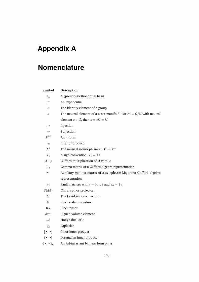
Appendix A
Nomenclature
Symbol Description
e
n A (pseudo-)orthonormal basis
ex An exponential
e The identity element of a group
o The neutral element of a coset manifold. For M = G/K with neutral
element e ∈ G, then o = eK = K
→ Injection
Surjection
P (n) An n-form
ιX Interior product
X[ The musical isomorphism [ : V → V ∗
κi A sign convention, κi = ±1
A · ψ Clifford multiplication of A with ψ
Γa Gamma matrix of a Clifford algebra representation
γi Auxiliary gamma matrix of a symplectic Majorana Clifford algebra
representation
σi Pauli matrices with i = 0 . . . 3 and σ0 = 12
P(±1) Chiral spinor projector
∇ The Levi-Civita connection
R Ricci scalar curvature
Ric Ricci tensor
dvol Signed volume element
?A Hodge dual of A
4 Laplacian
J·,·K Pinor inner product
L·,·M Lorentzian inner product
⟪·,·⟫m An Ad-invariant bilinear form on m
108
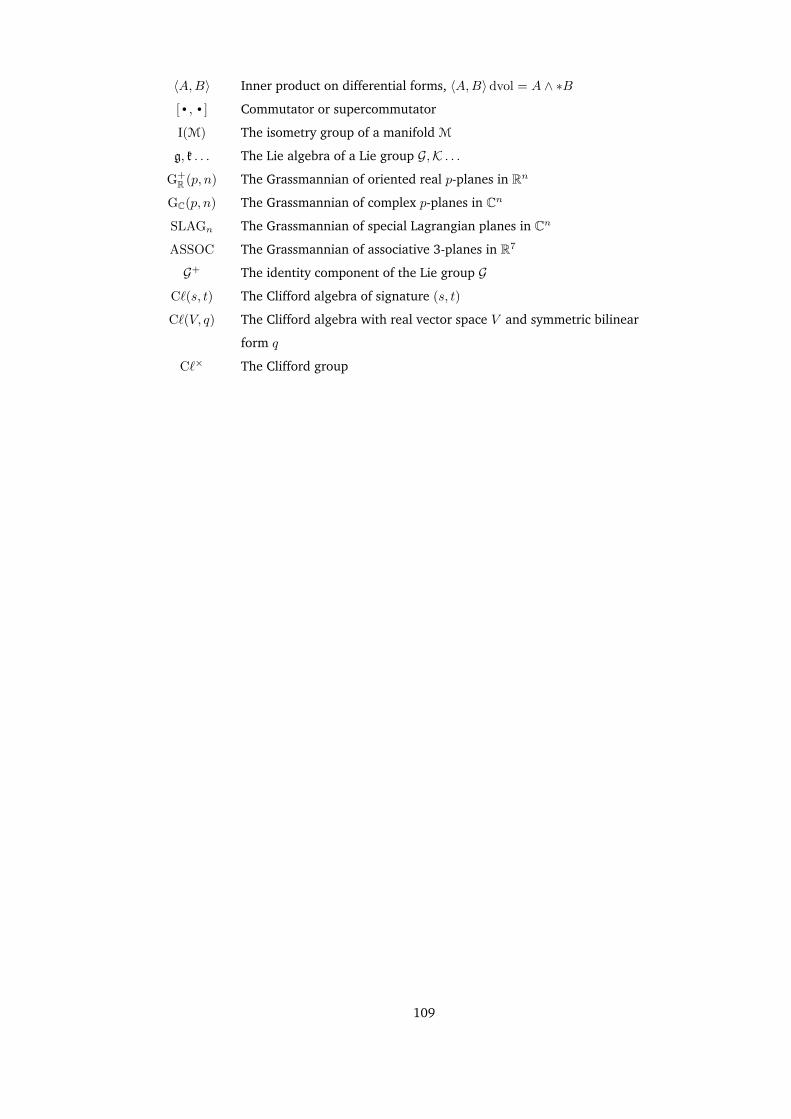
〈A,B〉 Inner product on differential forms, 〈A,B〉dvol = A ∧ ∗B
[·,·] Commutator or supercommutator
I(M) The isometry group of a manifold M
g, k . . . The Lie algebra of a Lie group G,K . . .
G+R (p, n) The Grassmannian of oriented real p-planes in Rn
GC(p, n) The Grassmannian of complex p-planes in Cn
SLAGn The Grassmannian of special Lagrangian planes in Cn
ASSOC The Grassmannian of associative 3-planes in R7
G+ The identity component of the Lie group G
C`(s, t) The Clifford algebra of signature (s, t)
C`(V, q) The Clifford algebra with real vector space V and symmetric bilinear
form q
C`× The Clifford group
109
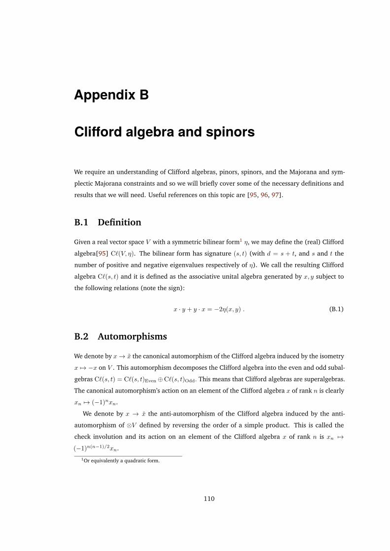
Appendix B
Clifford algebra and spinors
We require an understanding of Clifford algebras, pinors, spinors, and the Majorana and sym-
plectic Majorana constraints and so we will briefly cover some of the necessary definitions and
results that we will need. Useful references on this topic are [95, 96, 97].
B.1 Definition
Given a real vector space V with a symmetric bilinear form1 η, we may define the (real) Clifford
algebra[95] C`(V, η). The bilinear form has signature (s, t) (with d = s + t, and s and t the
number of positive and negative eigenvalues respectively of η). We call the resulting Clifford
algebra C`(s, t) and it is defined as the associative unital algebra generated by x, y subject to
the following relations (note the sign):
x · y + y · x = −2η(x, y) . (B.1)
B.2 Automorphisms
We denote by x→ x the canonical automorphism of the Clifford algebra induced by the isometry
x 7→ −x on V . This automorphism decomposes the Clifford algebra into the even and odd subal-
gebras C`(s, t) = C`(s, t)Even ⊕C`(s, t)Odd. This means that Clifford algebras are superalgebras.
The canonical automorphism’s action on an element of the Clifford algebra x of rank n is clearly
xn 7→ (−1)nxn.
We denote by x → x the anti-automorphism of the Clifford algebra induced by the anti-
automorphism of ⊗V defined by reversing the order of a simple product. This is called the
check involution and its action on an element of the Clifford algebra x of rank n is xn 7→
(−1)n(n−1)/2xn.
1Or equivalently a quadratic form.
110
We denote by x→ x the anti-automorphism of the Clifford algebra induced by the composi-
tion of x → x and x → x. This is called the hat involution and its action on an element of the
Clifford algebra x of rank n is xn 7→ (−1)n(n+1)/2xn.
B.3 Groups
The Clifford algebra contains three groups which are of interest: We start with the group of
invertible elements (the Clifford group) C`×(s, t) which must of course contain all other groups.
Then the Clifford group has two subgroups of more direct consequence:
• The Pin group (unital simple products):
Pin(s, t) = y ∈ C`(s, t) : y =∏n
xn with x2n = ±1 (B.2)
• The Spin group (unital simple products stabilised by the canonical automorphism):
Spin(s, t) = y ∈ C`(s, t) : y =∏n
xn with x2n = ±1 and n mod 2 = 0
= Pin(s, t) ∩ C`(s, t)Even
(B.3)
B.4 Representations
The Clifford algebra (as we have defined it) is a real associative algebra but we are interested
in complex representations and so a representation2 of a Clifford algebra C`(s, t) on a complex
vector space S is a homomorphism
ρ : C`(s, t)→ End(S) . (B.4)
We also then naturally have representations of the Pin and Spin subgroups of the Clifford
algebra, elements of which are pinors and spinors respectively.
B.4.0.1 Matrix ring isomorphisms
Clifford algebras themselves are (non-canonically) algebra-isomorphic to matrix rings or direct
sums of matrix rings over a field K as an algebra over R. The matrix dimension and field K
depend upon the signature mod 8 via Bott periodicity [98]. For a Clifford algebra C`(s, t) and
d = s+ t we have the algebra isomorphisms [96],
2A Clifford module
111
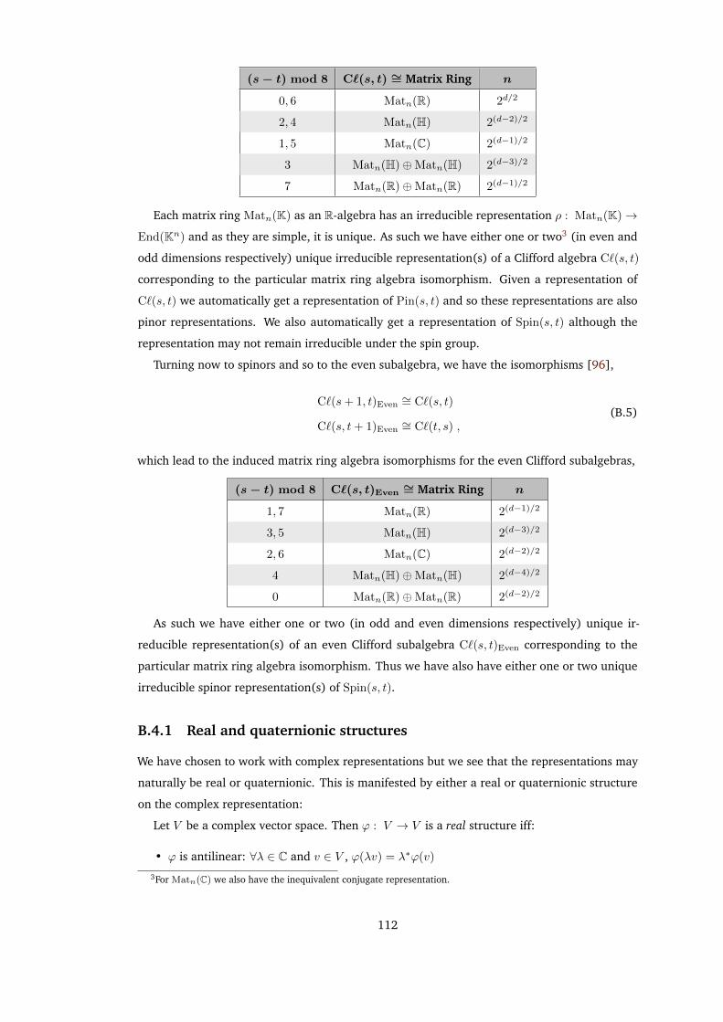
(s− t) mod 8 C`(s, t) ∼= Matrix Ring n
0, 6 Matn(R) 2d/2
2, 4 Matn(H) 2(d−2)/2
1, 5 Matn(C) 2(d−1)/2
3 Matn(H)⊕Matn(H) 2(d−3)/2
7 Matn(R)⊕Matn(R) 2(d−1)/2
Each matrix ring Matn(K) as an R-algebra has an irreducible representation ρ : Matn(K)→
End(Kn) and as they are simple, it is unique. As such we have either one or two3 (in even and
odd dimensions respectively) unique irreducible representation(s) of a Clifford algebra C`(s, t)
corresponding to the particular matrix ring algebra isomorphism. Given a representation of
C`(s, t) we automatically get a representation of Pin(s, t) and so these representations are also
pinor representations. We also automatically get a representation of Spin(s, t) although the
representation may not remain irreducible under the spin group.
Turning now to spinors and so to the even subalgebra, we have the isomorphisms [96],
C`(s+ 1, t)Even∼= C`(s, t)
C`(s, t+ 1)Even∼= C`(t, s) ,
(B.5)
which lead to the induced matrix ring algebra isomorphisms for the even Clifford subalgebras,
(s− t) mod 8 C`(s, t)Even∼= Matrix Ring n
1, 7 Matn(R) 2(d−1)/2
3, 5 Matn(H) 2(d−3)/2
2, 6 Matn(C) 2(d−2)/2
4 Matn(H)⊕Matn(H) 2(d−4)/2
0 Matn(R)⊕Matn(R) 2(d−2)/2
As such we have either one or two (in odd and even dimensions respectively) unique ir-
reducible representation(s) of an even Clifford subalgebra C`(s, t)Even corresponding to the
particular matrix ring algebra isomorphism. Thus we have also have either one or two unique
irreducible spinor representation(s) of Spin(s, t).
B.4.1 Real and quaternionic structures
We have chosen to work with complex representations but we see that the representations may
naturally be real or quaternionic. This is manifested by either a real or quaternionic structure
on the complex representation:
Let V be a complex vector space. Then ϕ : V → V is a real structure iff:
• ϕ is antilinear: ∀λ ∈ C and v ∈ V , ϕ(λv) = λ∗ϕ(v)
3For Matn(C) we also have the inequivalent conjugate representation.
112
• ϕ2 = 1 .
As an involution, a real structure has two eigenvalues ±1 and so decomposes V into two ei-
genspaces V = V+⊕V− and these eigenspaces are real because the structure map is not complex
linear but antilinear. A real structure ϕ is thus just an abstraction of complex conjugation.
Now, let V again be a complex vector space. Then ϕ : V → V is a quaternionic structure iff:
• ϕ is antilinear: ∀λ ∈ C and v ∈ V , ϕ(λv) = λ∗ϕ(v)
• ϕ2 = −1 .
Since ϕ2 = −1 and ϕ(iv) = −iϕ(v), the quaternionic structure defines a left quaternionic
j-action on V and so a left H-action on V : If H 3 q = a+bj for a, b ∈ C, we have qv = av+bϕ(v).
Of course, we are interested in pinor and spinor representations and so these structures
must be pin- or spin-invariant. For example, in signature (s − t) mod 8 = 1 we only have a
spin-invariant real structure and so only the spinor representation is real.
B.4.2 Majorana and symplectic Majorana spinors
With a spin-invariant real structure on our representation we can always choose a basis in which
this structure acts either as the identity (in which case we have concretely real Majorana spinors)
or as the imaginary identity (in which case we have purely imaginary pseudo-Majorana spinors).
For example,D = 11 supergravity may equally well be formulated with a spinor bundle modelled
upon C`(10, 1) [19] in which case we have (purely imaginary) pseudo-Majorana spinors or on
C`(1, 10) [35, 40] in which case we have (concretely real) Majorana spinors.
Unfortunately, in signatures (s− t) mod 8 = 3, 4, 5 we have no spin-invariant real structure
to work with. However, in these signatures we do always have spin-invariant quaternionic
structures. Let us start with a representation V of C`(s, t) with a quaternionic structure ϕ1 and
take some other auxiliary representation W of a group G that also has a quaternionic structure
ϕ2. We may construct the tensor product of representations V ⊗W which is a representation of
C`(s, t)×G. We then have a new structure ϕ1 ⊗ ϕ2 satisfying:
• ϕ1 ⊗ ϕ2 is antilinear: ∀λ ∈ C, v ∈ V , w ∈W ,
(ϕ1 ⊗ ϕ2)(λv ⊗ w) = (ϕ1(λv)⊗ ϕ2(w)) = (λ∗ϕ1(v)⊗ ϕ2(w)) = λ∗(ϕ1 ⊗ ϕ2)(v ⊗ w)
• (ϕ1 ⊗ ϕ2)2 = (ϕ21)⊗ (ϕ2
2) = (−1V )⊗ (−1W ) = 1V⊗W .
As such, the tensor product of two representations each with quaternionic structures is a new
representation with a real structure.
Using this construction, if we have a spinor representation with no real structure, then we
may combine it with an auxiliary quaternionic representation to create a real structure on a new
reducible representation. Given a choice of basis in which the new real structure acts as either
the identity or the imaginary identity, we then have concretely real symplectic Majorana spinors
113
or purely imaginary symplectic pseudo-Majorana spinors respectively. See appendices B.11.3
and B.11.4 for concrete examples of reducible symplectic Majorana representations.
B.4.3 Gamma matrices
A matrix representation of the Clifford algebra is concretely furnished by the gamma matrices
Γn,
ΓaΓb + ΓbΓa = 2κ1ηab1 , (B.6)
where κ1 = ±1 is a sign convention typically (but not strictly) chosen to be +1 in the physics
literature and −1 in the mathematics literature including [95]. Note that this does not change
our definition of the Clifford algebra equation (B.1) but merely enables us to make contact with
the conventions in the literature.
We define totally antisymmetric products of gamma matrices as
Γa1...an := Γ[a1 . . .Γan] . (B.7)
B.5 Exterior algebra isomorphism
We have the vector space isomorphism Λ(V ) ∼= C`(V ) concretely defined by
Λ(V )→ C`(V )
1
n!Xa1...an e
a1 ∧ . . . ∧
e
an 7→ Xa1...anΓa1...an .(B.8)
This isomorphism globalises to a vector bundle isomorphism between the exterior bundle
and the Clifford bundle. A spinor bundle is a bundle of Clifford modules by construction and
so we have a natural action of sections of the exterior bundle on sections of the spinor bundle
through this vector bundle isomorphism and the natural Clifford action on the spinor bundle.
Using this isomorphism, we have the following relations between the interior and exterior
products in the exterior algebra and the Clifford product in the Clifford algebra. So, for a vector
X ∈ V ∗ and n-form P ∈ Λn(V ) we have,
ιXP = 12κ1
(X[ · P − (−1)nP ·X[
)(B.9)
X[ ∧ P = 12
(X[ · P + (−1)nP ·X[
). (B.10)
114

B.6 Inner products
The two involutions of the Clifford algebra induce two pinor inner products on a pinor repres-
entation P such that
Jx · ε1, ε2K = Jε1, x · ε2K , (B.11)
where ε1,2 ∈ P and x denotes either the hat or the check involution of x ∈ C`(V ) ∼= End(P).
The inner products can take the form of any of the eight types of inner product on R, C, and
H depending on the matrix ring algebra isomorphism of the Clifford algebra:
• R: symmetric or symplectic
• C: symmetric, symplectic, hermitian symmetric, or hermitian symplectic
• H: hermitian symmetric or hermitian symplectic
Also, if there are two inequivalent pinor representations, an inner product may intertwine them
and thus only be defined on their direct sum.
B.7 Identities
B.7.1 Product identities
Rearranging the Clifford algebra definition on gamma matrices equation (B.6) yields
ΓaΓb = 2κ1η(a, b)1− ΓbΓa. (B.12)
This rearrangement can be iterated to yield the general product formula,
Γa1...anΓb1...bm =
min (n,m)∑t=0
t!
(n
t
)(m
t
)κ1
t(−1)t(2n+t+1)/2δ[a1[b1
. . . δatbt Γat+1...an]bt+1...bm] . (B.13)
B.7.2 Volume identities
We define the Clifford volume element of signature d = s+ t to be
Γvol := Γ1...d. (B.14)
As a consequence, we have
Γa1...anΓvol = (−1)n(d−1)ΓvolΓa1...an . (B.15)
Upon manipulation of equation (B.13), noting that only the t = n term is non-zero, we have
115
the more general identity
Γa1...anΓvol = κ1n(−1)n(n−1)/2 1
(d−n)!εa1...an,b1...bd−nΓb1...bd−n . (B.16)
Using the index formulation of the Hodge star operator on an n-form A,
(∗A)b1...bd−n= 1
(d−n)!Aa1...anεa1...an,b1...bd−n
, (B.17)
we arrive at the identity,
Aa1...anΓa1...anΓvol = κ1n(−1)n(n−1)/2(∗A)b1...bd−n
Γb1...bd−n . (B.18)
B.8 (Anti-)self-dual forms
In dimensions (s − t) mod 4 = 0 we may construct (anti-)self-dual forms ?Aκ2 = κ2Aκ2 . In
these dimensions the eigenvalues of Γvol are real and chiral spinors satisfy the relation
Γvolεκ3 = κ3ε
κ3 . (B.19)
We thus have the chirality projectors
P(κ3) = 12 (Γvol + κ31) , (B.20)
where P(κ3) projects the κ3 chirality subspace.
Then, for an (anti-)-self-dual n-form, equation (B.18) becomes
Aκ2a1...anΓa1...anΓvol = κ2κ1
n(−1)n(n−1)/2Aκ2a1...anΓa1...an , κ2Aa1...an (B.21)
and so
Aκ2a1...anΓa1...anP(κ2κ1
n(−1)n(n−1)/2+1) = 0 . (B.22)
We see that an (anti-)self-dual n-form thus annihilates κ2κ1n(−1)n(n−1)/2+1 chirality spinors.
Two relevant examples in Lorentzian signature:
• (s, t) = (5, 1): we have (anti-)self-dual 3-forms and, if using Clifford algebra sign κ1 = −1
we have
κ2κ1n(−1)n(n−1)/2+1 = κ2 · (−1)3 · (−1)3(3−1)/2+1 = −κ2 , (B.23)
meaning that in this case self-dual 3-forms annihilate negative chirality spinors and anti-
self-dual 3-forms annihilate positive chirality spinors.
• (s, t) = (1, 9): we have self-dual 5-forms and, if using Clifford algebra sign κ1 = −1 we
116
have
κ2κ1n(−1)n(n−1)/2+1 = κ2 · (−1)5 · (−1)5(5−1)/2+1 = κ2 , (B.24)
meaning that in this case self-dual 5-forms annihilate positive chirality spinors and anti-
self-dual 5-forms annihilate negative chirality spinors.
B.9 Covariant spinor derivative
We derive the form of the covariant spinor derivative so as to make clear how the sign adopted
in the definition of the Clifford algebra κ1 enters the definition.
We first suppose the covariant spinor derivative along a vectorX takes the form, for unknown
θ in the spin subalgebra,
∇Xε = ∂Xε+ θ(X) · ε . (B.25)
We then require the Leibniz condition be compatible with the Clifford action and so,
∇X(W · ε) = (∇XW ) · ε+W · ∇Xε . (B.26)
Substituting in our supposed form yields the condition, for any vectors W ,
θ(X) ·W −W · θ(X)!= ∇XW − ∂XW . (B.27)
We may then explicitly compute θ,
θ(X)abWc(ΓabΓc − ΓcΓab) = θ(X)abWc(−4κ1η
c[aΓb])
= −4κ1θ(X)abWaΓb
!= Xc(∂cWaΓa + ωc
abWbΓa − ∂cWaΓa)
= XcωcabWbΓa ,
(B.28)
where we have used the definition of the covariant derivative of a vector W in terms of the
spin connection ω,
∇µW a = ∂cWa + ωc
abWb . (B.29)
Thus we have
θ(X)ab = 14κ1X
cωcab , (B.30)
and so
∇Xε = ∂Xε+ 14κ1ωX · ε . (B.31)
117
B.10 Spinorial Lie derivative
We derive the form of the spinorial Lie derivative [39] so as to make clear how the sign adopted
in the definition of the Clifford algebra κ1 enters the definition.
We first suppose the spinorial Lie derivative along a Killing vector K takes the form, for
unknown θ in the Spin subalgebra,
LKε = ∇Kε+ θ(K) · ε . (B.32)
We then require the Leibniz condition be compatible with the Clifford action and so,
LK(W · ε) = [K,W ] · ε+W · LKε . (B.33)
Substituting in our supposed form yields the condition, for any vector W ,
θ(K) ·W −W · θ(K)!= −∇WK . (B.34)
We may then explicitly compute θ,
−W aΓb∇aKb!= θ(K)abWc(Γ
abΓc − ΓcΓab)
= θ(K)abWc(−4κ1ηc[aΓb])
= −4κ1θ(K)abWaΓb ,
(B.35)
whence
θ(K)ab = 14κ1∇aKb , (B.36)
and so
LKε = ∇Kε+ 14κ1(∇K) · ε . (B.37)
B.11 Explicit realisations of pinor representations
B.11.1 D = 11
In D = 11 we use sign conventions (see appendices B.4.3 and C) (κ0,κ1) = (−1,−1) or
(κ0,κ1) = (+1,+1) meaning we work with C`(1, 10). We use a Majorana representation con-
structed as
Γ0 = iσ1 ⊗ σ0 ⊗ σ0 ⊗ σ0 ⊗ σ2 Γ1 = σ1 ⊗ σ0 ⊗ σ0 ⊗ σ3 ⊗ σ3 Γ2 = σ1 ⊗ σ0 ⊗ σ0 ⊗ σ1 ⊗ σ3
Γ3 = σ2 ⊗ σ3 ⊗ σ2 ⊗ σ0 ⊗ σ0 Γ4 = σ2 ⊗ σ1 ⊗ σ2 ⊗ σ0 ⊗ σ0 Γ5 = σ2 ⊗ σ2 ⊗ σ0 ⊗ σ0 ⊗ σ0
Γ6 = σ1 ⊗ σ2 ⊗ σ1 ⊗ σ2 ⊗ σ3 Γ7 = σ1 ⊗ σ0 ⊗ σ2 ⊗ σ2 ⊗ σ3 Γ8 = σ1 ⊗ σ2 ⊗ σ3 ⊗ σ2 ⊗ σ3
Γ9 = σ1 ⊗ σ0 ⊗ σ0 ⊗ σ0 ⊗ σ1 Γ10 = σ3 ⊗ σ0 ⊗ σ0 ⊗ σ0 ⊗ σ0 .
118
The gamma matrices are all real and
Γvol := Γ0...10 = 1 . (B.38)
B.11.2 D = 10
In D = 10 we use sign conventions (κ0,κ1) = (−1,−1) meaning we work with C`(1, 9). We use
a Majorana-Weyl representation constructed as
Γ0 = iσ1 ⊗ σ0 ⊗ σ0 ⊗ σ0 ⊗ σ2 Γ1 = σ1 ⊗ σ0 ⊗ σ0 ⊗ σ3 ⊗ σ3 Γ2 = σ1 ⊗ σ0 ⊗ σ0 ⊗ σ1 ⊗ σ3
Γ3 = σ2 ⊗ σ3 ⊗ σ2 ⊗ σ0 ⊗ σ0 Γ4 = σ2 ⊗ σ1 ⊗ σ2 ⊗ σ0 ⊗ σ0 Γ5 = σ2 ⊗ σ2 ⊗ σ0 ⊗ σ0 ⊗ σ0
Γ6 = σ1 ⊗ σ2 ⊗ σ1 ⊗ σ2 ⊗ σ3 Γ7 = σ1 ⊗ σ0 ⊗ σ2 ⊗ σ2 ⊗ σ3 Γ8 = σ1 ⊗ σ2 ⊗ σ3 ⊗ σ2 ⊗ σ3
Γ9 = σ1 ⊗ σ0 ⊗ σ0 ⊗ σ0 ⊗ σ1 .
The gamma matrices are all real and
Γvol := Γ0...9 = σ3 ⊗ σ0 ⊗ σ0 ⊗ σ0 ⊗ σ0 . (B.39)
B.11.3 D = 6, (1, 0)
In D = 6, (1, 0) we use sign conventions (κ0,κ1) = (+1,−1) meaning we work with C`(5, 1).
We use a symplectic Majorana-Weyl representation constructed as
Γ0 = σ1 ⊗ σ0 ⊗ σ0 ⊗ σ1 Γ1 = iσ1 ⊗ σ0 ⊗ σ2 ⊗ σ3 Γ2 = iσ2 ⊗ σ3 ⊗ σ0 ⊗ σ0
Γ3 = iσ2 ⊗ σ2 ⊗ σ2 ⊗ σ0 Γ4 = iσ1 ⊗ σ0 ⊗ σ0 ⊗ σ2 Γ5 = iσ2 ⊗ σ1 ⊗ σ0 ⊗ σ0 .
The gamma matrices are all real and
Γvol := Γ0...5 = σ3 ⊗ σ0 ⊗ σ0 ⊗ σ0 . (B.40)
The auxiliary representation of C`(3, 0) is then
γ1 = iσ0 ⊗ σ0 ⊗ σ2 ⊗ σ0 γ2 = iσ3 ⊗ σ2 ⊗ σ1 ⊗ σ3 γ3 = iσ3 ⊗ σ2 ⊗ σ3 ⊗ σ3 .
The auxiliary gamma matrices are all real and
γiγj + γjγi =− 2δij1 , (B.41)
γi =γi , (B.42)
γvol :=γ1...3 = 1 , (B.43)
[Γa, γi] =0 . (B.44)
B.11.4 D = 6, (2, 0)
In D = 6, (2, 0) we use sign conventions (κ0,κ1) = (+1,−1) meaning we work with C`(5, 1).
We use a symplectic Majorana-Weyl representation constructed as
119
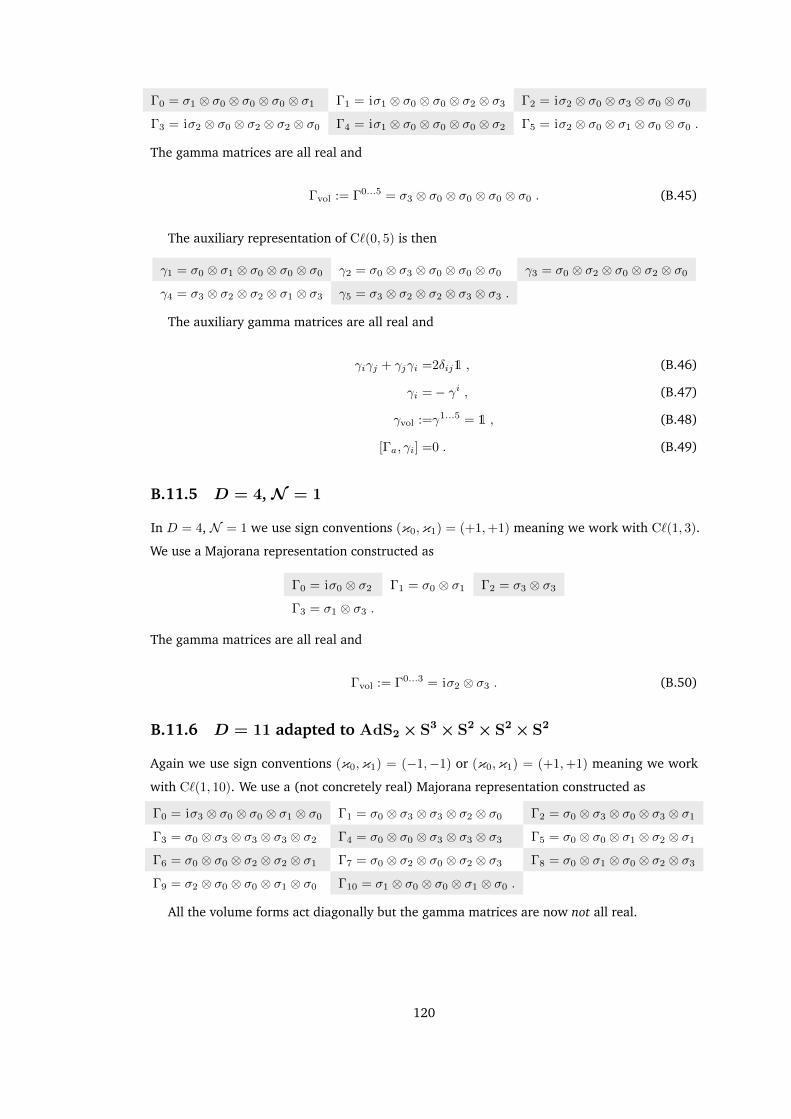
Γ0 = σ1 ⊗ σ0 ⊗ σ0 ⊗ σ0 ⊗ σ1 Γ1 = iσ1 ⊗ σ0 ⊗ σ0 ⊗ σ2 ⊗ σ3 Γ2 = iσ2 ⊗ σ0 ⊗ σ3 ⊗ σ0 ⊗ σ0
Γ3 = iσ2 ⊗ σ0 ⊗ σ2 ⊗ σ2 ⊗ σ0 Γ4 = iσ1 ⊗ σ0 ⊗ σ0 ⊗ σ0 ⊗ σ2 Γ5 = iσ2 ⊗ σ0 ⊗ σ1 ⊗ σ0 ⊗ σ0 .
The gamma matrices are all real and
Γvol := Γ0...5 = σ3 ⊗ σ0 ⊗ σ0 ⊗ σ0 ⊗ σ0 . (B.45)
The auxiliary representation of C`(0, 5) is then
γ1 = σ0 ⊗ σ1 ⊗ σ0 ⊗ σ0 ⊗ σ0 γ2 = σ0 ⊗ σ3 ⊗ σ0 ⊗ σ0 ⊗ σ0 γ3 = σ0 ⊗ σ2 ⊗ σ0 ⊗ σ2 ⊗ σ0
γ4 = σ3 ⊗ σ2 ⊗ σ2 ⊗ σ1 ⊗ σ3 γ5 = σ3 ⊗ σ2 ⊗ σ2 ⊗ σ3 ⊗ σ3 .
The auxiliary gamma matrices are all real and
γiγj + γjγi =2δij1 , (B.46)
γi =− γi , (B.47)
γvol :=γ1...5 = 1 , (B.48)
[Γa, γi] =0 . (B.49)
B.11.5 D = 4, N = 1
In D = 4, N = 1 we use sign conventions (κ0,κ1) = (+1,+1) meaning we work with C`(1, 3).
We use a Majorana representation constructed as
Γ0 = iσ0 ⊗ σ2 Γ1 = σ0 ⊗ σ1 Γ2 = σ3 ⊗ σ3
Γ3 = σ1 ⊗ σ3 .
The gamma matrices are all real and
Γvol := Γ0...3 = iσ2 ⊗ σ3 . (B.50)
B.11.6 D = 11 adapted to AdS2× S3× S2× S2× S2
Again we use sign conventions (κ0,κ1) = (−1,−1) or (κ0,κ1) = (+1,+1) meaning we work
with C`(1, 10). We use a (not concretely real) Majorana representation constructed as
Γ0 = iσ3 ⊗ σ0 ⊗ σ0 ⊗ σ1 ⊗ σ0 Γ1 = σ0 ⊗ σ3 ⊗ σ3 ⊗ σ2 ⊗ σ0 Γ2 = σ0 ⊗ σ3 ⊗ σ0 ⊗ σ3 ⊗ σ1
Γ3 = σ0 ⊗ σ3 ⊗ σ3 ⊗ σ3 ⊗ σ2 Γ4 = σ0 ⊗ σ0 ⊗ σ3 ⊗ σ3 ⊗ σ3 Γ5 = σ0 ⊗ σ0 ⊗ σ1 ⊗ σ2 ⊗ σ1
Γ6 = σ0 ⊗ σ0 ⊗ σ2 ⊗ σ2 ⊗ σ1 Γ7 = σ0 ⊗ σ2 ⊗ σ0 ⊗ σ2 ⊗ σ3 Γ8 = σ0 ⊗ σ1 ⊗ σ0 ⊗ σ2 ⊗ σ3
Γ9 = σ2 ⊗ σ0 ⊗ σ0 ⊗ σ1 ⊗ σ0 Γ10 = σ1 ⊗ σ0 ⊗ σ0 ⊗ σ1 ⊗ σ0 .
All the volume forms act diagonally but the gamma matrices are now not all real.
120
Appendix C
Sign conventions
We have seen in appendix B.4.3 that we have a choice of sign κ1 = ±1 to make when con-
structing a gamma matrix representation of the Clifford algebra. There is yet another choice of
sign available in the physics literature and this is the sign convention of the Lorentzian metric
tensor. We can either pick it to be mostly plus or mostly minus corresponding to the sign of the
majority of the eigenvalues of the metric tensor as a matrix. This is often historically called
picking an east-coast or west-coast sign and there is discussion [99] over whether one or the
other is preferable. We will denote this sign choice by κ0 = ±1 where κ0 = +1 denotes a mostly
plus metric and κ0 = −1 mostly minus.
In most applications the choice of metric sign κ0 is irrelevant [100, 101] but the combination
of (κ0,κ1) imposes a choice of pinor representation [102] and this can have consequences
because although change of metric sign is an isomorphism of spinor representations, the pinor
representations are not isomorphic.
We will not delve into this any further, but will specify our sign conventions where necessary
and in some cases try to present sign-agnostic results.
121
Appendix D
Lorentzian vector spaces
We recite a few simple facts about Lorentzian vector spaces.
D.1 Causal character
Taking a Lorentzian vector space V , let us denote its Lorentzian inner product by L·,·M and
choose a pseudo-orthonormal basis esuch that −L e
0,
e
0M = L e
i,
e
iM = κ0 and L e
0,
e
iM = L e
i,
e
jM =
0 for i > 0 6= j > 0.
A vector v ∈ V may be characterised as:
• Timelike: κ0Lv, vM < 0
• Null: κ0Lv, vM = 0
• Spacelike: κ0Lv, vM < 0 ,
(D.1)
and we add two further descriptions for utility:
• Causal: κ0Lv, vM ≤ 0
• Anti-causal: κ0Lv, vM ≥ 0 .(D.2)
D.2 Some results on null subspaces
Inner product of linearly independent null vectors
Let us take two linearly independent null vectors vi with i = 1, 2. Without loss of generality, with
respect to a pseudo-orthonormal basis we have vi = ai
e
0 + ui with ai real non-zero constants,
and ui spacelike vectors.
Let us suppose that Lv1, v2M = 0. Thus 0 = Lv1, v2M = κ0 (−a1a2 + Lu1, u2M) and so Lu1, u2M =
a1a2. Also 0 = Lvi, viM = κ0
(−a2
i + Lui, uiM)
and so Lui, uiM = a2i . But then we have Cauchy-
Schwarz equality |Lu1, u2M|2 = Lu1, u1MLu2, u2M meaning that u2 = λu1 for some non-zero λ.
122
Then a1a2 = Lu1, u2M = λLu1, u1M = λa21 and so a2 = λa1. But then v2 = λa1
e
0 + λu1 = λv1
contradicting linear independence. Thus Lv1, v2M 6= 0.
A totally null subspace is at most one-dimensional
Let us assume we have a totally null subspace with dimension greater than one. Then we
have at least two linearly independent null vectors v1 and v2. From polarisation we have that
Lv1 + v2, v1 + v2M = 2Lv1, v2M but from the inner product of linearly independent null vectors we
know that Lv1, v2M 6= 0 and so Lv1 + v2, v1 + v2M 6= 0 meaning v1 + v2 is not null and thus the
subspace is not totally null. Thus a totally null subspace is at most one-dimensional.
The perpendicular complement of a totally null subspace contains only
itself and spacelike vectors
The perpendicular complement of a subspace W ⊂ V with respect to the Lorentzian inner
product is defined as
W⊥ = v ∈ V : Lv, wM = 0 ∀ w ∈W , (D.3)
but a totally null subspace W is at most one-dimensional and so if non-trivial is spanned by
a single null vector w. Its perpendicular complement is thus
W⊥ = v ∈ V : Lv, wM = 0 . (D.4)
Now, Lw,wM = 0 and so w ∈W⊥ but we have seen that for vn a null vector linearly independ-
ent of w, Lvn, wM 6= 0 and so vn /∈W⊥.
Let us now take our null vector w and any timelike vector vt. Without loss of generality, with
respect to a pseudo-orthonormal basis we can write these as w = a e
0 +ws and vt = b e
0, for a, b
real non-zero constants. Then Lvt, wM = κ0ab 6= 0 and so also vt /∈W⊥.
Thus we see that the perpendicular complement of a totally null subspace contains only itself
and spacelike vectors.
123
Bibliography
[1] José Figueroa-O’Farrill and Noel Hustler. ‘The homogeneity theorem for supergravity
backgrounds’. Journal of High Energy Physics 2012.10 (2012) (cit. on pp. ii, 12, 26, 29,
32, 93).
[2] José Figueroa-O’Farrill and Noel Hustler. ‘The homogeneity theorem for supergravity
backgrounds II: the six-dimensional theories’. Journal of High Energy Physics 2014.4
(2014) (cit. on pp. ii, 12, 26, 37, 38, 41, 93).
[3] José Figueroa-O’Farrill and Noel Hustler. ‘Symmetric backgrounds of type IIB supergrav-
ity’. Classical and Quantum Gravity 30.4 (2013) (cit. on pp. ii, 62, 96).
[4] Noel Hustler and Andree Lischewski. ‘(M-theory-)Killing spinors on symmetric spaces’.
Journal of Mathematical Physics 56.8 (2015) (cit. on pp. ii, 96, 97).
[5] Albert Einstein. ‘Die Feldgleichungen der Gravitation’. Sitzungsberichte der Königlich
Preußischen Akademie der Wissenschaften (1915) (cit. on p. 1).
[6] Robert M. Wald. General Relativity. University of Chicago Press, 1984 (cit. on p. 1).
[7] B. P. Abbott et al. ‘Observation of Gravitational Waves from a Binary Black Hole Merger’.
Physical Review Letters 116.6 (2016) (cit. on p. 1).
[8] Steven Weinberg. The Quantum Theory of Fields: Volume 1, Foundations. Cambridge
University Press, 2005 (cit. on p. 1).
[9] Gordon McCabe. The Structure and Interpretation of the Standard Model. 2007 (cit. on
p. 1).
[10] ATLAS Collaboration. ‘Observation of a new particle in the search for the Standard
Model Higgs boson with the ATLAS detector at the LHC’. Physics Letters B 716.1 (2012)
(cit. on p. 2).
[11] CMS Collaboration. ‘Observation of a new boson at a mass of 125 GeV with the CMS
experiment at the LHC’. Physics Letters B 716.1 (2012) (cit. on p. 2).
[12] Planck Collaboration et al. ‘Planck 2013 results. I. Overview of products and scientific
results’. Astronomy & Astrophysics 571 (2014) (cit. on p. 2).
[13] Sidney Coleman and Jeffrey Mandula. ‘All Possible Symmetries of the S Matrix’. Phys.
Rev. 159 (5 1967) (cit. on p. 2).
124
[14] Steven Weinberg. The Quantum Theory of Fields: Volume 3, Supersymmetry. Cambridge
University Press, 2005 (cit. on p. 2).
[15] Daniel Z Freedman and Antoine Van Proeyen. Supergravity. Cambridge University Press,
2012 (cit. on p. 3).
[16] Yoshiaki Tanii. Introduction to Supergravity. Vol. 1. December. 2014 (cit. on p. 3).
[17] Daniel Z. Freedman, P. van Nieuwenhuizen and S. Ferrara. ‘Progress toward a theory of
supergravity’. Phys. Rev. D 13 (12 1976) (cit. on p. 3).
[18] S. Deser and B. Zumino. ‘Consistent supergravity’. Physics Letters B 62.3 (1976) (cit. on
p. 3).
[19] E. Cremmer, B. Julia and J. Scherk. ‘Supergravity in theory in 11 dimensions’. Physics
Letters B 76.4 (1978) (cit. on pp. 3, 26, 62, 113).
[20] J. Scherk and John H. Schwarz. ‘Dual models for non-hadrons’. Nuclear Physics B 81.1
(1974) (cit. on p. 3).
[21] Joseph Polchinski. String Theory, Vols. 1 & 2. Cambridge University Press, 2005 (cit. on
p. 3).
[22] Dean Rickles. A Brief History of String Theory. The Frontiers Collection. Berlin, Heidel-
berg: Springer Berlin Heidelberg, 2014 (cit. on p. 3).
[23] Michael B. Green and John H. Schwarz. ‘Anomaly cancellations in supersymmetric D =
10 gauge theory and superstring theory’. Physics Letters B 149.1 (1984) (cit. on p. 3).
[24] Ralph Blumenhagen et al. ‘TOWARD REALISTIC INTERSECTING D-BRANE MODELS’.
Annual Review of Nuclear and Particle Science 55.1 (2005) (cit. on p. 3).
[25] JIN DAI, R.G. LEIGH and JOSEPH POLCHINSKI. ‘NEW CONNECTIONS BETWEEN
STRING THEORIES’. Modern Physics Letters A 04.21 (1989) (cit. on p. 3).
[26] Michael B. Green. ‘Space-time duality and Dirichlet string theory’. Physics Letters B
266.3 (1991) (cit. on p. 3).
[27] Edward Witten. ‘String theory dynamics in various dimensions’. Nuclear Physics B
443.1-2 (1995) (cit. on pp. 3, 63).
[28] Andreas Arvanitoyeorgos. An Introduction to Lie Groups and the Geometry of Homogen-
eous Spaces. Vol. 22. The Student Mathematical Library. American Mathematical Society,
2003 (cit. on p. 5).
[29] Theodore Frankel. The geometry of physics: an introduction. 3rd ed. Cambridge Univer-
sity Press, 2011 (cit. on p. 6).
[30] Michel Cahen and N Wallach. ‘Lorentzian symmetric spaces’. Bulletin of the American
Mathematical Society 76.3 (1970) (cit. on pp. 9, 96).
[31] M Cahen and M Parker. ‘Parallélismes absolus des variétés lorentziennes’. Ann. Inst.
Fourier (Grenoble) 27 (1977) (cit. on pp. 9, 96).
125
[32] Sigurdur Helgason. Differential Geometry, Lie Groups, and Symmetric Spaces. American
Mathematical Society, 2001 (cit. on pp. 9, 96).
[33] José Figueroa-O’Farrill. ‘Symmetric M-theory backgrounds’. Open Physics 11.1 (2013)
(cit. on pp. 9, 62, 73, 96, 99–104).
[34] José Figueroa-O’Farrill. ‘The homogeneity conjecture for supergravity backgrounds’.
Journal of Physics: Conference Series 175 (2009) (cit. on pp. 12, 21, 93).
[35] José Figueroa-O’Farrill, Patrick Meessen and Simon Philip. ‘Supersymmetry and homo-
geneity of M-theory backgrounds’. Classical and Quantum Gravity 22.1 (2005) (cit. on
pp. 12, 26, 29, 113).
[36] Robert Geroch. ‘Limits of spacetimes’. Communications in Mathematical Physics 13
(1969) (cit. on pp. 13, 67, 103).
[37] Bertram Kostant. ‘Holonomy and the Lie algebra of infinitesimal motions of a Rieman-
nian manifold’. Transactions of the American Mathematical Society 80.2 (1955) (cit. on
p. 13).
[38] M. Scheunert. The theory of Lie superalgebras: an introduction. Springer-Verlag, 1979
(cit. on p. 16).
[39] Yvette Kosmann. ‘Dérivées de Lie des spineurs’. Annali di Matematica Pura ed Applicata,
Series 4 91.1 (1971) (cit. on pp. 16, 118).
[40] Jerome P Gauntlett and Stathis Pakis. ‘The geometry of D = 11 Killing spinors’. Journal
of High Energy Physics 2003.04 (2003) (cit. on pp. 26, 113).
[41] José Figueroa-O’Farrill, Emily Hackett-Jones and George Moutsopoulos. ‘The Killing su-
peralgebra of 10-dimensional supergravity backgrounds’. Classical and Quantum Gravity
24.13 (2007) (cit. on pp. 29, 32).
[42] J Schwarz. ‘Covariant field equations of chiral N = 2 D = 10 supergravity’. Nuclear
Physics B 226.2 (1983) (cit. on pp. 29, 62).
[43] John H. Schwarz and P.C. West. ‘Symmetries and transformations of chiral N = 2, D =
10 supergravity’. Physics Letters B 126.5 (1983) (cit. on pp. 29, 62, 64).
[44] P.S. Howe and P.C. West. ‘The complete N =2, d = 10 supergravity’. Nuclear Physics B
238.1 (1984) (cit. on pp. 29, 62).
[45] Emily J. Hackett-Jones and Douglas J Smith. ‘Type IIB Killing spinors and calibrations’.
Journal of High Energy Physics 2004.11 (2004) (cit. on p. 29).
[46] G.F. Chapline and N.S. Manton. ‘Unification of Yang-Mills theory and supergravity in
ten dimensions’. Physics Letters B 120.1-3 (1983) (cit. on p. 32).
[47] Ali H. Chamseddine. ‘N = 4 supergravity coupled to N = 4 matter and hidden symmet-
ries’. Nuclear Physics B 185.2 (1981) (cit. on p. 32).
126
[48] Lars Brink, John H. Schwarz and J. Scherk. ‘Supersymmetric Yang-Mills theories’. Nuc-
lear Physics B 121.1 (1977) (cit. on p. 32).
[49] Ulf Gran et al. ‘Geometry of all supersymmetric type I backgrounds’. Journal of High
Energy Physics 2007.08 (2007) (cit. on p. 32).
[50] Michael B. Green and John H. Schwarz. ‘Anomaly cancellations in supersymmetric D =
10 gauge theory and superstring theory’. Physics Letters B 149.1-3 (1984) (cit. on p. 33).
[51] Jan B. Gutowski, Dario Martelli and Harvey S. Reall. ‘All supersymmetric solutions of
minimal supergravity in six dimensions’ (2003) (cit. on p. 37).
[52] H Nishino and E Sezgin. ‘Matter and gauge couplings of N= 2 supergravity in six
dimensions’. Physics Letters B 144.3 (1984) (cit. on p. 38).
[53] Ali Chamseddine, José Figueroa-O’Farrill and Wafic Sabra. ‘Supergravity vacua and
lorentzian Lie groups’ (2003) (cit. on p. 41).
[54] PK Townsend. ‘A new anomaly free chiral supergravity theory from compactification on
K3’. Physics Letters B 139.4 (1984) (cit. on p. 41).
[55] Yoshiaki Tanii. ‘N= 8 supergravity in six dimensions’. Physics Letters B 145.3 (1984)
(cit. on p. 41).
[56] Daniel Z. Freedman, P. van Nieuwenhuizen and S. Ferrara. ‘Progress toward a theory of
supergravity’. Physical Review D 13.12 (1976) (cit. on p. 46).
[57] S. Deser and B. Zumino. ‘Consistent supergravity’. Physics Letters B 62.3 (1976) (cit. on
p. 46).
[58] K.S. Stelle and P.C. West. ‘Minimal auxiliary fields for supergravity’. Physics Letters B
74.4-5 (1978) (cit. on p. 46).
[59] S. Ferrara and P. van Nieuwenhuizen. ‘The auxiliary fields of supergravity’. Physics
Letters B 74.4-5 (1978) (cit. on p. 46).
[60] Ulf Gran, J Gutowski and George Papadopoulos. ‘Geometry of all supersymmetric four-
dimensional 𝒩 = 1 supergravity backgrounds’. Journal of High Energy Physics
2008.06 (2008) (cit. on p. 46).
[61] M.J. Duff, B.E.W. Nilsson and C.N. Pope. ‘Kaluza-Klein supergravity’. Physics Reports
130.1-2 (1986) (cit. on p. 50).
[62] M.J. Duff. ‘Kaluza-Klein Theory in Perspective’. The Oskar Klein centenary. October
1994. 1994 (cit. on p. 50).
[63] Josep M. Pons and Pere Talavera. ‘Consistent and inconsistent truncations. Some results
and the issue of the correct uplifting of solutions’. Nuclear Physics B 678.1-2 (2004)
(cit. on p. 50).
[64] P.M. Saffin. ‘Type IIA Killing spinors and calibrations’. Physical Review D 71.2 (2005)
(cit. on p. 54).
127
[65] H. Nishino and E. Sezgin. ‘The complete N = 2, d = 6 supergravity with matter and
yang-mills couplings’. Nuclear Physics B 278.2 (1986) (cit. on p. 56).
[66] Emesto Lozano-Tellechea, Patrick Meessen and Tomás Ortín. ‘On d = 4, 5, 6 vacua with
8 supercharges’. Classical and Quantum Gravity 19.23 (2002) (cit. on p. 56).
[67] Giovanni Calvaruso. ‘Homogeneous structures on three-dimensional Lorentzian mani-
folds’. Journal of Geometry and Physics 57.4 (2007) (cit. on p. 62).
[68] B.B. Komrakov. ‘Einstein-Maxwell equation on four-dimensional homogeneous spaces’.
Lobachevskii Journal of Mathematics 8 (2001) (cit. on p. 62).
[69] Nadine Kowalsky. ‘Noncompact Simple Automorphism Groups of Lorentz Manifolds and
Other Geometric Manifolds’. The Annals of Mathematics 144.3 (1996) (cit. on p. 62).
[70] Mohamed Deffaf, Karin Melnick and Abdelghani Zeghib. ‘Actions of Noncompact
Semisimple Groups on Lorentz Manifolds’. Geometric and Functional Analysis 18.2
(2008) (cit. on p. 62).
[71] D. V. Alekseevsky. ‘Homogeneous Lorentzian manifolds of a semisimple group’. Journal
of Geometry and Physics 62.3 (2012) (cit. on p. 62).
[72] Michael B. Green and John H. Schwarz. ‘Supersymmetrical string theories’. Physics
Letters B 109.6 (1982) (cit. on p. 62).
[73] F. Giani and M. Pernici. ‘N = 2 supergravity in ten dimensions’. Physical Review D 30.2
(1984) (cit. on p. 62).
[74] I.C.G. Campbell and P.C. West. ‘N = 2, D = 10 non-chiral supergravity and its spontan-
eous compactification’. Nuclear Physics B 243.1 (1984) (cit. on p. 62).
[75] M. Huq and M.A. Namazie. ‘Kaluza-Klein supergravity in ten dimensions’. Classical and
Quantum Gravity 2.4 (1985) (cit. on p. 62).
[76] Jin Dai, R.G. Leight and Joseph Polchinski. ‘New connections between string theories’.
Modern Physics Letters A 04.21 (1989) (cit. on p. 62).
[77] M. Dine, P. Huet and N. Seiberg. ‘Large and small radius in string theory’. Nuclear
Physics B 322.2 (1989) (cit. on p. 62).
[78] A. Font et al. ‘Strong-weak coupling duality and non-perturbative effects in string theory’.
Physics Letters B 249.1 (1990) (cit. on p. 62).
[79] John H. Schwarz. ‘An SL (2, Z) multiplet of type IIB superstrings’. Physics Letters B
364.4 (1995) (cit. on pp. 62, 64).
[80] Juan Maldacena. ‘The Large-N Limit of Superconformal Field Theories and Supergravity’.
International Journal of Theoretical Physics 38.4 (1999) (cit. on p. 63).
[81] Chris Hull and P.K. Townsend. ‘Unity of superstring dualities’. Nuclear Physics B 438.1-2
(1995) (cit. on p. 64).
128
[82] E. Cremmer and B. Julia. ‘The SO(8) supergravity’. Nuclear Physics B 159.1-2 (1979)
(cit. on p. 64).
[83] Daniel Lazard. ‘Thirty years of Polynomial System Solving, and now?’ Journal of Sym-
bolic Computation 44.3 (2009) (cit. on p. 67).
[84] Noel Hustler. ‘The homogeneity theorem for supergravity backgrounds III: dimensional
reductions’. Unpublished (2015) (cit. on p. 93).
[85] U Gran, J Gutowski and G Papadopoulos. ‘M-theory backgrounds with 30 Killing spinors
are maximally supersymmetric’. Journal of High Energy Physics 2010.3 (2010) (cit. on
p. 94).
[86] José Figueroa-O’Farrill. Presentation: Killing superalgebras in supergravity. Tech. rep.
2008 (cit. on p. 94).
[87] U Gran et al. ‘IIB solutions with N>28 Killing spinors are maximally supersymmetric’.
Journal of High Energy Physics 2007.12 (2007) (cit. on p. 94).
[88] Jeremy Michelson. ‘A pp-wave with 26 supercharges’. Classical and Quantum Gravity
19.23 (2002) (cit. on p. 94).
[89] Robert L Bryant. Isometry group of a homogeneous space. MathOverflow. 2011 (cit. on
p. 94).
[90] José Figueroa-O’Farrill. ‘Homogeneous M2 Duals’. Unpublished (2013) (cit. on p. 94).
[91] S Kobayashi and K Nomizu. Foundations of differential geometry. Vol. I. Wiley, 1996
(cit. on p. 97).
[92] S Kobayashi and K Nomizu. Foundations of differential geometry. Vol. II. Wiley, 1996
(cit. on p. 97).
[93] Matthias Hammerl. ‘Homogeneous Cartan Geometries’. PhD thesis. Universitaet Wien,
2006 (cit. on p. 97).
[94] K.D. Kirchberg. ‘The first eigenvalue of the Dirac operator on Kähler manifolds’. Journal
of Geometry and Physics 7.4 (1990) (cit. on p. 100).
[95] F Reese Harvey. Spinors and Calibrations. Academic Press Inc, 1990 (cit. on pp. 110,
114).
[96] H Blaine Lawson and Marie-Louise Michelsohn. Spin geometry. Princeton University
Press, 1989 (cit. on pp. 110–112).
[97] José Figueroa-O’Farrill. Majorana spinors (cit. on p. 110).
[98] M.F. Atiyah, R. Bott and A. Shapiro. ‘Clifford modules’. Topology 3.9 (1964) (cit. on
p. 111).
[99] Peter Woit. The West Coast Metric is the Wrong One (cit. on p. 121).
129
[100] M.J. Duff and J. Kalkkinen. ‘Signature reversal invariance’. Nuclear Physics B 758.1-2
(2006) (cit. on p. 121).
[101] M.J. Duff and J. Kalkkinen. ‘Metric and coupling reversal in string theory’. Nuclear
Physics B 760.1-2 (2007) (cit. on p. 121).
[102] Marcus Berg et al. ‘The pin groups in physics: C, P and T’. Reviews in Mathematical
Physics 13.08 (2001) (cit. on p. 121).
130

I never look back darling, it distracts from the now.
131


![Supersymmetric Gauge Theory with Space-time Dependent ...arXiv:1710.09792v2 [hep-th] 1 Feb 2018 YITP-17-113 Supersymmetric Gauge Theory with Space-time Dependent Couplings Jaewang](https://img.dokumen.tips/doc/110x75/5e77abeb96af705b671d36a4/supersymmetric-gauge-theory-with-space-time-dependent-arxiv171009792v2-hep-th.jpg)


![Aspects of Supersymmetric Guage Theory and String Theory [Thesis] - M. Huang (2004) WW](https://img.dokumen.tips/doc/110x75/577d1d101a28ab4e1e8b88b2/aspects-of-supersymmetric-guage-theory-and-string-theory-thesis-m-huang.jpg)


![Black Holes In Supergravity And String Theory - [jnl article] - T. Mohaupt (2000) WW.pdf](https://img.dokumen.tips/doc/110x75/552afe384a79598c118b461c/black-holes-in-supergravity-and-string-theory-jnl-article-t-mohaupt-2000-wwpdf.jpg)


