Home production as a substitute to market consumption?

Estimating the elasticity using houseprice shocks from the Great

Recession ∗

Jim Been † Susann Rohwedder ‡ Michael Hurd §

July 2015

Abstract

The theory of home production suggests that people will substitute away from market consumption asthe opportunity cost of time drops. This makes people able to smooth consumption in response to shocksin income. Prior studies have investigated the effect of a drop in the cost of time on home production byanalyzing shocks of retirement, unemployment and disability. Such shocks both decrease the householdsmonetary budget and increase the time budget. Hence, home production responses are the cumulativeeffect of decreased market consumption and increased non-market time available. The current papercontributes to the literature by estimating the intratemporal elasticity between home production andmarket consumption. Wealth shocks in houseprices induced by the Great Recession are used to infer theextent to which households adjusted home production in response to decreasing market consumptionpossibilities. By using a panel data set with detailed information on both consumption spending andtime use, we find that a 10% decrease in substitutable consumption spending increases home productionactivities by about 6.5%. Although the scope in substitutability is rather limited, there are non-negligiblepossibilities to substitute away from market consumption to home production. This is in contrast withthe high substitutability assumed in existing theoretical models of home production.

JEL codes: D12, D13, D91, J22, J26Keywords: Home production, Time use, Consumption, Wealth shocks, Great Recession

∗The work was supported by a grant from the Social Security Administration through the Michigan Retirement ResearchCenter (Grant #RRC08098401−06). This paper was written while Jim was a Visiting Researcher at the RAND Center for theStudy on Aging at RAND. This research visit has been sponsored by Leiden University Fund/ van Walsem (Grant #4414/3−9−13\V,vW ) and the Leiden University Department of Economics. We have benefited from discussions with Marco Angrisani,Yoosoon Chang, Arie Kapteyn, Marike Knoef, Lieke Kools, Italo Lopez-Garcia and Robert Willis. Furthermore, we wouldlike to thank the participants at the 21st International Panel Data Conference, 29-30 June 2015, Budapest. The findingsand conclusions expressed are solely those of the authors and do not represent the opinions or policy of the Social SecurityAdministration, any agency of the Federal government, or the Michigan Retirement Research Center.

†Department of Economics at Leiden University and Netspar (e-mail address: j.been@law.leidenuniv.nl)‡RAND Corp., Santa Monica, CA, USA, MEA and Netspar (e-mail address: susannr@rand.org)§RAND Corp., Santa Monica, CA, USA, NBER, MEA and Netspar (e-mail address: mhurd@rand.org)

1 Introduction

In his seminal work, Becker (1965) argues that consumption is ‘produced’ by two inputs: market ex-

penditures (market consumption) and time (home production). Whether the chosen consumption bundle

exists of relatively many market expenditures or time depends on the relative price of time. The price

of time, which is the wage foregone by spending time in non-market work, determines market expendi-

ture. Hence, spending on market consumption is a bad proxy for actual consumption as ‘time’ can be

used to increase consumption beyond market spending (Aguiar & Hurst, 2005). To the extent possible,

market consumption can be substituted by time without changing well-being. Moreover, the theory of

home production of Becker (1965) suggests that people will substitute away from market consumption

as the opportunity cost of time drops. Both intertemporarily and intratemporarily (Aguiar et al., 2012).

Shifting away from market consumption to home production makes people able to smooth consumption

in response to shocks in income (Hicks, 2015).

Firstly, the drop in consumption spending at retirement that was long assumed to be inconsistent

with the predictions of the Life-Cycle Hypothesis known as the retirement consumption puzzle,1 may

be explained by the increases in total time spent in home production during retirement. Hurst (2008)

finds a large heterogeneity in spending changes at retirement across different categories of consumption.

Especially food expenditures are found to fall sharply relative to other consumption components at

retirement (Aguila et al., 2011; Hurd & Rohwedder, 2013; Velarde & Herrmann, 2014). Aguiar &

Hurst (2005) explain this phenomenon by showing that retired persons use their additionally available

non-market time to substitute purchased goods and services (e.g. dining out) for home production (e.g.

cooking). Stancanelli & Van Soest (2012) show that the act of retirement increases time spent in home

production activities next to food-related activities. So, home production makes people partially able to

mitigate the consequences of retirement for well-being.

Secondly, it is found that time spent in home production activities is higher in households with un-

employed individuals than in households with employed individuals (Ahn et al., 2008; Burda & Hamer-

mesh, 2010; Taskin, 2011; Colella & Van Soest, 2013; Velarde & Herrmann, 2014). Conversely, Krueger

1Found by, among others, Mariger (1987); Robb & Burbidge (1989); Banks et al. (1998); Bernheim et al. (2001); Miniaciet al. (2003); Battistin et al. (2009).

2

& Mueller (2012) find sharp drops in home production at the time of reemployment. Hence, home pro-

duction is found to fluctuate over the business cycle (Benhabib et al., 1991; Greenwood & Hercowitz,

1991; Rupert et al., 2000; Hall, 2009; Karabarbounis, 2014) as people become unemployed or reem-

ployed. Burda & Hamermesh (2010) explicitly find evidence that individuals generally offset market

hours with home production during times of high cyclical unemployment. Griffith et al. (2014) find that

households lowered food spending by increased shopping effort during the Great Recession. Aguiar et

al. (2013) find that about 30% of lost working hours were absorbed by home production during the Great

Recession. So, home production makes people partially able to mitigate the consequences of unemploy-

ment for well-being. Home production is even partially able to mimic the role of formal unemployment

insurance as Guler & Taskin (2013) suggest.

Thirdly, shocks in health are found to have consequences for time spent in home production. Health

shocks increase the total non-work time available, but may also decrease the healthy non-work time

available. Gimenez-Nadal & Ortega-Lapiedra (2013) find a negative relationship between health and

time devoted to home production activities in Spain, e.g. people with a relatively poor health spent

more hours in home production. In contrast, Halliday & Podor (2012) find that improvements to health

increase time spent in home production activities in the US. Despite the fact that health has consequences

for time spent in home production, the extent to which home production makes people partially able to

mitigate the consequences of a health shock for consumption remains unclear.

The aforementioned shocks causing a drop in the opportunity cost of time (retirement, unemploy-

ment, disability) have two simultaneous effects 1) it decreases the monetary budget and 2) it increases

the time budget. The monetary budget is decreased by the difference in earnings (wage times market

hours) and social insurance (pension, unemployment benefits, disability benefits respectively) causing a

drop in available income for consumption expenditures. The time budget is increased as retired, unem-

ployed and disabled persons have considerably more non-market time available. However, prior studies

do not distinguish these two effects such that the substitution between market consumption and home

production found is a cumulative effect of the elasticity of home production to consumption spending

and home production to non-market time.

3

Focusing on food expenditures of Mexican prime age workers, Hicks (2015) has estimated a (semi-

)elasticity between home production and consumption spending possibilities.2 By estimating the effect

of permanent income on different food categories that differ in time needed to produce the food, Hicks

(2015) finds a negative effect of permanent income on home production. Despite the fact that using per-

manent income solves the problems with the time budget, identification comes from differences between

poorer and richer persons. Identifying within person responses using transitory shocks are, like previous

studies, modeled using unemployment thereby introducing the problem of a non-constant time budget.

Compared to prior studies, the current paper identifies the intratemporal substitution effect between

market consumption and home production from differences within a person over time, while keeping

the time budget constant. This would be a direct measure of the extent to which individuals can smooth

consumption while facing a shock in income. As time spent in home production and consumption

spending is determined simultaneously, we identify the elasticity by the drop in houseprices observed

during the Great Recession as a wealth shock. The drop in houseprices during the Great Recession were

unexpected and sufficiently substantial to decrease the monetary budget. Angrisani et al. (2013) and

Christelis et al. (2015) find substantial decreases in consumption spending due to the drop in houseprices.

At the same time, there is no reason to expect to that this shock in wealth changed the total time available

for home production.3 Therefore, the responses in home production due to drops in houseprice, as

analyzed by Kuehn (2015), should be caused by their effect on the monetary budget in stead of the time

budget. Kuehn (2015) does not differentiate between the two effects which may explain the ambiguity

of his results.

We use a unique panel data set with detailed information on both consumption- and time-use cate-

gories produced by combining the HRS with CAMS data for the years 2005-2011. To the best of our

knowledge there is only a handful of papers that uses panel data with detailed information on both con-

sumption spending and time use. The data in (Colella & Van Soest, 2013) is such an example but is

restricted to the Netherlands for the period 2009-2012. Some home production papers only have infor-

2The Mexican ENIGH data used in Hicks (2015) is a cross-sectional data set. We focus on all spending categories for U.S.persons aged 51 and over using panel data.

3This assumption holds conditionally on the assumption that the houseprice drops during Great Recession are not associatedwith increases in total time available. However, we know that the Great Recession induced unemployment. Therefore, we onlyselect retired individuals for our empirical analysis since these persons’ time budget did not change during the Great Recession.

4

mation regarding time use (Burda & Hamermesh, 2010; Aguiar et al., 2013). Data with information on

both consumption and time use are often imperfect because of a cross-sectional setting (Ahn et al., 2008)

or because of a focus on a very specific expenditure such as food (Velarde & Herrmann, 2014; Griffith

et al., 2014; Hicks, 2015).

We find an elasticity of home production with respect to market spending of -0.65. The elasticity is

mostly driven by persons with a drop in the value of their relatively cheap home that is free of mortgage

and who spent relatively much on market consumption that can be substituted for by home production

prior to the Great Recession. Contrasting existing theoretical models of home production that typically

assume high substitutability between market consumption and home production (Campbell & Ludvig-

son, 2001),4 we conclude that the scope of substituting market spending for home production is fairly

small. This implies that most of the home production responses found by earlier studies are primarily

the consequence of increased non-market time available.

The remainder of the paper is organized as follows. Section 2 describes the HRS and CAMS data

used in the paper. Descriptive statistics of time use and consumption spending are presented in Sec-

tion 3. To analyze home production formally, Section 4 presents a simple life-cycle model with home

production and wealth shocks. The functional form and the empirical model are derived in Section 5

and Section 6 respectively. The results of the empirical model are shown in Section 7. Conclusions

regarding the substitutability of home production and market consumption can be found in Section 8.

2 Data

The data for our empirical analyses come from the Health and Retirement Study (HRS), a longitudi-

nal survey that is representative of the U.S. population over the age of 50 and their spouses. The HRS

conducts core interviews of about 20,000 persons every two years. In addition the HRS conducts supple-

mentary studies to cover specific topics beyond those covered in the core surveys. The time use data we

use in this paper were collected as part of such a supplementary study, the Consumption and Activities

4Baxter & Jermann (1999) indicate that a plausible range of the elasticity would be between 0 and 5. Aguiar et al. (2012)describe that most of the estimated elasticities exceed 1 in the literature. However, micro estimates seem to produce somewhatsmaller elasticities than macro estimates. A commonly assumed benchmark in theoretical models is 3 (Greenwood et al., 1995;Baxter & Jermann, 1999), while an elasticity of 5 is used as well (Benhabib et al., 1991).

5

Mail Survey (CAMS).

Health and Retirement Study Core interviews

The first wave of the HRS was fielded in 1992. It interviewed people born between 1931 and 1941 and

their spouses, irrespective of age. The HRS re-interviews respondents every second year. Additional

cohorts have been added so that beginning with the 1998-wave the HRS is representative of the entire

population over the age of 50. The HRS collects detailed information on the health, labor force participa-

tion, economic circumstances, and social well-being of respondents. The survey dedicates considerable

time to elicit income and wealth information, providing a complete inventory of the financial situation

of households. In this study we use demographic and asset and income data from the HRS core waves

spanning the years 2002 through 2010.

Consumption and Activities Mail Survey

The CAMS survey aims to obtain detailed measures of time use and total annual household spending on

a subset of HRS respondents. These measures are merged to the data collected on the same households

in the HRS core interviews. The CAMS surveys are conducted in the HRS off-years, that is, in odd-

numbered years.

The first wave of CAMS was collected in 2001 and it has been collected every two years since. Ques-

tionnaires are sent out in late September or early October. Most questionnaires are returned in October

and November. CAMS thus obtains a snap-shot of time use observed in the fall of the CAMS survey

year. In the first wave, 5,000 households were chosen at random from the entire pool of households who

participated in the HRS 2000 core interview. Only one person per household was chosen. About 3,800

HRS households responded, so CAMS 2001 was a survey of the time-use of 3,800 respondents and the

total household spending of the 3,800 households in which these respondents live. Starting in the third

wave of CAMS, both respondents in a couple household were asked to complete the time use section,

so that the number of respondent-level observations on time use in each wave was larger for the waves

from 2005 and onwards.

Respondents were asked about a total of 31 time-use categories in wave 1; wave 2 added two more

categories; wave 4 added 4 additional categories. Thus, since CAMS 2007 the questionnaire elicits 37

6

time-use categories, as shown in Appendix A. Of particular interest for this study are the CAMS time

use categories related to home production:

• House cleaning

• Washing, ironing or mending clothes

• Yard work or gardening

• Shopping or running errands

• Preparing meals and cleaning up afterwards

• Taking care of finances or investments, such as banking, paying bills, balancing the checkbook,

doing taxes, etc.

• Doing home improvements, including painting, redecorating, or making home repairs

• Working on, maintaining, or cleaning car(s) and vehicle(s)

For most activities respondents are asked how many hours they spent on this activity last week. For less

frequent categories they were asked how many hours they spent on these activities last month. Hurd &

Rohwedder (2008) provide a detailed overview of the time use section of CAMS, its design features

and structure, and descriptive statistics. A detailed comparison of time use as recorded in CAMS with

that recorded in the American Time Use Survey (ATUS) shows summary statistics that are fairly close

across the two surveys, despite a number of differences in design and methodology (Hurd & Rohwedder,

2007).

In this paper we use data from CAMS 2005, 2007, 2009 and 2011, each wave containing between

about 5,300 and 6,500 respondent-level observations on time use that we merge with HRS core data.

Combining the data from the HRS core and the CAMS provides us with data that are unique in that

we observe demographics, economic status, time-use and spending for the same individuals and their

households in panel.

The data for this study come from the HRS. In 2001, the HRS added a supplemental survey eliciting

details of household spending, the Consumption and Activities Mail Survey (CAMS). Since then the

7

CAMS has been collected every two years (odd-numbered years) in the years between the core HRS

interviews. For the 2001 CAMS sample some 5,000 HRS households were randomly selected from

participants in the HRS 2000 core interview. As new cohorts were added to the HRS in 2004 and 2010 a

random subsample of the new households was again added to the CAMS sample for subsequent CAMS

data collections. The sample is representative for the US population over the age of 50.

The CAMS questionnaire consists of two parts: Part A asks about time use in about 35 categories

and Part B asks about household spending in about 40 categories. For couples, the main respondent

who fills out both sections of the survey is chosen at random and encouraged to solicit help from other

household members in completing the questions about household spending. The respondent fills out

the time use section referring only to his or her own personal time-use while the spending questions on

spending ask about the spending of the entire household. Starting in 2005, a spouse questionnaire was

added for couples which requested that the spouse fill out the time use questions referring to his or her

personal time use.

In this study we will therefore use CAMS data from 2005, 2007, 2009 and 2011 where we have time

use data on both spouses for couples. The CAMS data can be linked to the rich background information

that respondents provide in the HRS core interviews. Rates of item nonresponse are very low (mostly

single-digit), and CAMS spending totals aggregate closely to those in the CEX (Hurd & Rohwedder,

2009). The time use part of CAMS elicits time spent last week in 20 activities, and time spent last month

in 13 additional activities, and the number of days on trips or vacation over the past year. These time use

data aggregate closely to categories of time use in the American Time Use Study (Hurd & Rohwedder,

2007).

3 Descriptive statistics

3.1 Consumption

Table 1 shows the household spending on consumption that can be substituted for by home production.

The waves prior to the Great Recession show that spending is on average more substantial than in the

waves after the Great Recession. Interestingly, comparing wave 2007 to wave 2009 shows that total

8

consumption spending decreased by about 6% while total substitutable consumption decreased by about

17%. This larger drop in substitutable consumption implies that households’ spending on substitutable

consumption has a stronger cyclical reaction than total consumption. That is because households may

have found it easier to shift away from market consumption that well substitutable by home production.

Substitutable consumption is about 11-12% of total consumption spending and is consistent across

waves. This makes the substitutable consumption spending a non-negligible part of total consumption

spending. The biggest component of the substitutable consumption spending consists of dining out ex-

penditures. This expenditure could be well substituted for by home production in the form of cooking.

Standard deviations of the spending categories are relatively big compared to the mean. The relative size

of the standard deviation compared to the mean is much smaller for the total of consumption spending.

This suggest that there is especially large heterogeneity in consumption spending that could be substi-

tuted for by home production activities. We observe that virtually all households have expenditures that

could be substituted for by home production although the percentage of households with spending on

substitutable consumption decreased in later waves.

9

Tabl

e1:

Hou

seho

ldle

velc

onsu

mpt

ion

spen

ding

(US

dolla

rspe

ryea

r)a

Wav

e20

05W

ave

2007

Wav

e20

09W

ave

2011

Mea

nS.

D.

%To

tal

%H

ouse

hold

sM

ean

S.D

.%

Tota

l%

Hou

seho

lds

Mea

nS.

D.

%To

tal

%H

ouse

hold

sM

ean

S.D

.%

Tota

l%

Hou

seho

lds

Din

ing

out

1,91

23,

530

4.7

85.0

1,80

82,

912

4.5

84.5

1,51

32,

096

4.0

83.9

1,59

82,

443

4.4

81.2

Hou

seke

epin

gse

rvic

es41

41,

194

1.0

49.3

386

1,05

41.

049

.533

198

41.

045

.234

91,

014

1.0

43.4

Gar

deni

ngse

rvic

es38

11,

371

1.0

34.2

355

1,17

91.

033

.831

483

31.

035

.629

685

40.

833

.5H

omer

epai

rser

vice

s1,

347

3,92

33.

349

.81,

465

6,51

53.

748

.51,

068

2,82

92.

848

.41,

006

3,53

42.

843

.2V

ehic

lem

aint

enan

ce64

987

51.

683

.061

480

41.

581

.661

880

91.

680

.459

883

31.

678

.2D

ishw

ashe

r23

115

0.0

4.4

2712

70.

05.

019

105

0.0

3.6

1591

0.0

3.5

Was

hing

/Dry

ing

mac

hine

6325

00.

08.

776

293

0.0

9.7

6827

80.

09.

253

232

0.0

8.3

Subs

titut

able

cons

umpt

ion

4,78

86,

633

11.8

964,

730

8,25

311

.995

3,93

14,

748

10.5

953,

915

5,55

710

.894

Subs

titut

able

cons

umpt

ion

excl

.dur

able

s4,

703

6,59

011

.696

4,62

78,

201

11.6

953,

844

4,70

010

.295

3,84

75,

515

10.6

93Su

bstit

utab

leco

nsum

ptio

nin

cl.s

uppl

.mat

.6,

487

8,06

916

.099

6,38

79,

878

16.0

995,

342

5,79

514

.299

5,38

27,

071

14.8

98

Tota

lcon

sum

ptio

n40

,558

29,4

2710

010

039

,904

29,2

6810

010

037

,515

25,7

7810

010

036

,359

26,0

8610

010

0

aM

onet

ary

mea

sure

sar

eex

pres

sed

in20

11U

Sdo

llars

usin

gth

eC

onsu

mer

Pric

eIn

dex

ofth

eB

urea

uof

Lab

orSt

atis

tics.

10

3.2 Time use

Table 2 shows the time spent in home production activities per wave by persons aged 51-80. These

activities can be used as a substitute for the market bought goods and services shown in Table 1. The

aggregate of home production activities shows that a non-negligible part of the weekly available time

is spent on home production and that virtually all persons engage in some form of home production.

Hence, issues regarding left-censoring of the home production variable are negligible.

Most of the home production is devoted to the cooking of meals. Together with the house cleaning,

this accounts for about half of total time spent in home production. More than 80% of the persons in

the data spend some time on these two home production activities. About 90% of the people engage in

shopping activities although the average time spent in this activity is somewhat smaller than the time

spent in house cleaning and cooking. Unlike activities such as house cleaning, cooking and doing the

laundry, it is harder to buy the service for shopping on the market which may explain the relatively high

percentage of persons engaging in this activity. Approximately half of the people engage in gardening

and maintenance of the home and vehicles but the amount of time spent in these activities are fairly

small. More than 80% of the people spend time on managing their finances, but the amount of time

spent in this activity is only about an hour per week.

Despite the fact that a non-negligible part of the weekly available time is devoted to home production

activities on average, there is a lot of variation around this average as the standard deviations of most

activities are about the same size as the averages (or even bigger). However, the variation across waves

is only marginal despite the observed drop in substitutable market consumption in Table 1. This might

suggest that people do not adjust their time use in home production that much during the course of the

business cycle.

11

Tabl

e2:

Tim

e-us

ein

hom

epr

oduc

tion

activ

ities

(hou

rspe

rwee

k)

Wav

e20

05W

ave

2007

Wav

e20

09W

ave

2011

Mea

nS.

D.

%To

tal

%R

espo

nden

tsM

ean

S.D

.%

Tota

l%

Res

pond

ents

Mea

nS.

D.

%To

tal

%R

espo

nden

tsM

ean

S.D

.%

Tota

l%

Res

pond

ents

Hou

secl

eani

ng4.

76.

321

.280

.84.

87.

122

.082

.14.

76.

121

.983

.04.

86.

522

.283

.3L

aund

ry2.

63.

711

.772

.92.

74.

712

.472

.92.

63.

712

.173

.92.

64.

012

.072

.8G

arde

ning

2.2

4.9

9.9

50.4

2.2

4.2

10.1

52.4

2.3

4.5

10.7

51.9

2.2

4.7

9.3

49.4

Shop

ping

3.9

4.9

17.6

88.5

3.8

4.7

17.4

87.4

3.8

4.5

17.7

89.1

3.8

4.2

17.6

88.1

Coo

king

6.4

6.9

28.8

85.8

6.3

7.2

28.9

85.9

6.3

6.6

29.3

86.7

6.2

6.6

28.7

86.2

Fina

ncia

lman

agem

ent

1.0

2.1

4.5

85.6

1.0

2.0

4.6

83.5

0.8

1.4

3.7

83.4

0.9

1.6

4.2

83.3

Hom

em

aint

enan

ce1.

03.

04.

545

.80.

82.

03.

744

.20.

72.

53.

340

.10.

72.

23.

239

.2V

ehic

lem

aint

enan

ce0.

40.

91.

852

.10.

30.

71.

851

.70.

30.

91.

448

.50.

41.

11.

948

.6

Hom

epr

oduc

tion

22.2

19.4

100

98.5

21.8

21.1

100

98.1

21.5

17.7

100

97.9

21.6

20.1

100

98.4

12

Together, Table 2 and Table 1 give some idea on the scope of substituting market purchases for

home production activities. To capture the possible substitution effects between the two more formally,

we present a life-cycle model with home production in the next section.

4 Model

4.1 A simple Life-Cycle Model with Home Production

The extension of the life-cycle model to allow for complementarity or substitutability between time

and consumption proposed by Laitner & Silverman (2005) reduces to the standard life-cycle model for

persons whose leisure is fixed (retirees, unemployed, disabled). Since our identifying assumption is a

non-changing time budget available, we need to explicitly incorporate home production in the life-cycle

model following Becker (1965); Gronau (1977); Apps & Rees (1997); Rupert et al. (2000); Apps &

Rees (2005). This introduces home produced goods cnt next to the classical market consumption cmt and

leisure lt such that individuals maximize

Uτ = maxEτ

[T

∑t=τ

(1+ρ)τ−tu(cmt ,cnt(hnt), lt)ψ(vt)

](1)

where ct and lt denote consumption and leisure in time period t, respectively. ρ is the discount factor and

T the time horizon of the household. vt are the personal- and household characteristics that influence

utility directly known as taste-shifters (e.g. age, household size, number of children). cnt(hnt) = gt(hnt)

is being the home production function with time spent in home production hnt . For simplicity, we

assume that the home production function is strictly concave in one variable input,5 namely the time

spent in home production. Individuals maximize Equation 1 under the time budget and monetary budget

constraint respectively

hmt = H− lt −hnt (2)

At+1 = (1+ r)(At +(wt ·hmt)+bt − cmt) (3)

5Relaxing this assumption would give cnt(hnt) = gt(xt ,hnt) with xt as market purchased inputs used in home production.Working with this relaxed assumption would give an additional expenditure term in the budget constraint.

13

AT ≥ 0 (4)

where At is the amount of assets at time t, r is a constant real interest rate, wt is the (after-tax) wage rate,

H the total time-endowment (e.g. 24 hours per day) and bt are benefits (e.g. pensions, unemployment

benefits, disability benefits and other unearned non-asset income).

Solving equation 1 subject to equations 3 and 2 gives the following Euler Equations of marginal

utility with respect to cmt (market goods), hnt (home production) and hmt (market production).

ucmt (cmt ,cnt(hnt), lt)ψ(vt) =

(1+ r1+δ

)Et [ucmt+1(cmt+1,cnt+1(hnt+1), lt+1)ψ(vt+1)] (5)

uhmt (cmt ,cnt(hnt), lt)ψ(vt) =−wt

(1+ r1+δ

)Et[uhmt+1(cmt+1,cnt+1(hnt+1), lt+1)ψ(vt+1)

](6)

uhnt (cmt ,cnt(hnt), lt)ψ(vt) = wt

(1+ r1+δ

)Et[uhnt+1(cmt+1,cnt+1(hnt+1), lt+1)ψ(vt+1)

](7)

where( 1+r

1+δ

)Et [ucmt+1(cmt+1,cnt+1(hnt+1), lt+1)ψ(vt+1)] captures the marginal utility of wealth. In other

words, the optimal level of consumption of market goods is where the marginal utility of consumption

of market goods equals the marginal utility of wealth (taking into account a fixed interest rate and

discount factor). The marginal utility of wealth takes into account all future expectations. Similarly, the

marginal utility of market production and home production depend on the marginal utility of wealth as

well as the wage rate. A higher wage rate, however, increases the marginal utility of market production

and decreases the marginal utility of home production for which the wage rate is an opportunity cost.

The model predicts that the marginal utility of market production and home production is equal across

different activities.

Expressions 5 and 7 imply that market consumption and home production are functions of the indi-

vidual’s current characteristics that determine the wage as well as all relevant information about other

periods, including future periods. To see this, introducing an expectation error εt+1 allows us to rewrite

the Euler Equations into

14

ucmt (cmt+1,cnt+1(hnt+1), lt+1)ψ(vt+1) =

(1+δ

1+ r

)ucmt (cmt ,cnt(hnt), lt)ψ(vt)+ εt+1 (8)

uhmt (cmt+1,cnt+1(hnt+1), lt+1)ψ(vt+1) =−wt

(1+δ

1+ r

)uhmt (cmt ,cnt(hnt), lt)ψ(vt)+ εt+1 (9)

uhnt (cmt+1,cnt+1(hnt+1), lt+1)ψ(vt+1) = wt

(1+δ

1+ r

)uhnt (cmt ,cnt(hnt), lt)ψ(vt)+ εt+1 (10)

where εt+1 is uncorrelated with all the information available at time t. The rewritten expressions ex-

plicitly show the recursive nature of the marginal utility of wealth in which only an unanticipated shock

(εt+1) can result into a deviation from the optimal path. This implies that the marginal utility of wealth

at time t is a function of (in our case) a constant representing the ratio between the interest rate and

the discount rate as well as a term that captures the individual specific effects (e.g. fixed effects) and a

random error that reflects the expectational error up to the current period. We use these facts to derive

our empirical model later.

4.2 A simple Life-Cycle Model with Home Production and Wealth Shocks

Since we are explicitly interested in how a wealth shock affects home production through its effect on

the monetary budget constraint, we add a stochastic component to the deterministic life-cycle monetary

budget constraint in Equation 3.

At+1 = (1+ r)(Et [At ]+ (wt ·hmt)+bt − cmt) (11)

with

Et [At ] = At +ξt (12)

where ξt yields a random term with Et [ξt ] = 0 that captures a shock in the value of wealth available at

time t. We assume Et [ξt ] = 0 in the marginal utility of wealth. A negative shock (ξt < 0) causes the

market consumption possibilities cmt+1 at time t +1 to decrease because ∆At+1 < 0. Hence, individuals

15

reoptimize hmt+1, hnt+1 and cmt+1 to the ξt < 0 accordingly in order to maximize Equation 1. ξt < 0

allows us to analyze ∆hnt+1∆cmt+1

in a situation of ∆cmt+1 < 0 and ∆hmt+1 = 0. This rules out that the change in

home production is a consequence of having more time available for home production. In stead, ∆hnt+1∆cmt+1

measures the true substitution effect between market consumption and home production.

In contrast, a shock of retirement, unemployment or disability would result in wt = 0, hmt = 0 and

bt ≥ 0. Therefore, ∆hnt+1 can be the result of both ∆cmt+1 < 0 and ∆hmt+1 < 0, e.g. the change in home

production is ∆hnt+1∆cmt+1

+ ∆hnt+1∆lt+1

.

5 A functional form to derive the empirical model

For simplicity, the functional form representation of preferences for market consumption, home produc-

tion and leisure is an additive utility function such that preferences are additively separable.6 A similar

simple functional form of the utility function was used by Rupert et al. (2000) and Gortz (2006). Kuehn

(2015) uses a multiplicative utility function with home production. More sophisticated functional forms

are used in Benhabib et al. (1991), Greenwood & Hercowitz (1991), Fang & Zhu (2012), Dotsey et al.

(2010), Rogerson & Wallenius (2013) and Karabarbounis (2014). These papers use a Cobb-Douglas

period utility function as a CES parameterization of the utility function with home production.7 Alessie

& De Ree (2008) also allow for a functional form that distinguishes between husband’s and wife’s home

production.

As we only intend to derive our empirical model from the life-cycle model with home production,

6We assume additively separable preferences in this framework to keep the derivation of our empirical model tractable. Inpractice, it is likely that the marginal utility of consumption does depend on home production, for example.

7This parameterization looks as follows.

u(cmt ,cnt(hnt), lt) =

(c1−b

t lbt

)1−φ

−1

1−φ(13)

with

ct =((1−a)cκ

mt +acκnt)1/κ (14)

Here, κ is the willingness to substitute between market consumption and home production. Market goods and home producedgoods are substitutes if κ < 1. φ is the willingness to substitute leisure and consumption. A consequence of this specificationin relation to our specification is that the marginal utility of consumption (either market or home produced) depends on theamount of leisure as well and vice versa.

16

it suffices to use the following simple functional form of the utility function as used by Gortz (2006)

where market consumption, home production and leisure are summed over spouses (e.g. joint decision-

making).8 Most importantly, this simple parameterization provides the expected negative relationship

between wages and home production which suggests that the opportunity cost of home production equals

the wage thereby introducing home production as a substitute to market consumption.

u(cmt ,cnt(hnt), lt) = cθmtmt + cnt(hnt)

θnt + lθltt (15)

with θmt , θnt and θlt being the preference parameters for market consumption, home production and

leisure such that θmt + θnt + θlt = 1. Productivity in home production cnt(hnt) = gt(hnt) is assumed to

have constant economies of scale but is assumed to be different over time:9 cnt(hnt) = gt(hnt) = γthnt

with γt being a positive parameter.

Inserting the derivative of Equation 15 with respect to market consumption, home production and

leisure into the Euler Equation (Equation 5-7) and using hmt = H− lt−hnt gives the following first-order

approximations of the Euler Equations of market consumption, home production and market production

given that the solution is interior.10

θmtc(θmt−1)mt ψ(vt) =

(1+ r1+δ

)Et

[θmt+1c(θmt+1−1)

mt+1 ψ(vt+1)]

(16)

θlth(θlt−1)mt ψ(vt) =−wt

(1+ r1+δ

)Et

[θlt+1h(θlt+1−1)

mt+1 ψ(vt+1)]

(17)

8Deriving the empirical model from using the Cobb-Douglas period utility function as a functional form would result ina reduced form model with extra parameters a, b, φ, ρ and marginal utility of consumption that depends on leisure and viceversa.

9In this way, productivity does not increase nor decrease with the number of hours of home production supplied, but canincrease or decrease over time because of, for example, aging or shocks in health. The assumption of constant economiesof scale has no constraining consequences for our empirical model, but allows us to neatly write down the derivation of theempirical model.

10To allow for corner solutions, such as people in retirement without labor supply (hmt = 0), equations 16-18 can be adjustedby multiplying the righthandside with e(−πRt ) (Deaton, 1971). Rt = 1 if a person is retired and zero otherwise. π is thedegree to which a person adjusts the marginal utility of market production and home production. π > 0 is assumed such that0 < e(−πRt ) < 1 if a person is retired meaning that the marginal utility of market production and home production does nothave to equal the marginal wage rate times the marginal utility of wealth as would be in interior solutions. Since we explicitlycondition the regression equations on the subsample of retired persons we do not explicitly account for the interior solution inthe derivation of the model.

17

θntγth(θnt−1)nt ψ(vt) = wt

(1+ r1+δ

)Et

[θnt+1γt+1h(θnt+1−1)

nt+1 ψ(vt+1)]

(18)

The log-linear approximation of Equation 16-18 gives

ln(θmt)+(θmt −1)ln(cmt)+ ln(ψ(vt)) =

ln(1+ r)− ln(1+δ)+Et [ln(θmt+1)+(θmt+1−1)ln(cmt+1)+ ln(ψ(vt+1))] (19)

ln(θlt)+(θlt −1)ln(hmt)+ ln(ψ(vt)) =

− ln(wt)+ ln(1+ r)− ln(1+δ)+Et [ln(θlt+1)+(θlt+1−1)ln(hmt+1)+ ln(ψ(vt+1))] (20)

ln(γt)+ ln(θnt)+(θnt −1)ln(hnt)+ ln(ψ(vt)) =

ln(wt)+ ln(1+ r)− ln(1+δ)+Et [ln(γt+1)+ ln(θnt+1)+(θnt+1−1)ln(hnt+1)+ ln(ψ(vt+1))] (21)

Using 8-10 this yields11

∆ln(cmt+1) =1

∆(θmt+1−1)(ln(1+ r)− ln(1+δ)+∆ln(θmt+1)+∆ln(ψ(vt+1)))+ εt+1 (22)

∆ln(hmt+1) =

1∆(θmt+1−1)

(−ln(wt)+ ln(1+ r)− ln(1+δ)+∆ln(θmt+1)+∆ln(ψ(vt+1)))+ εt+1 (23)

∆ln(hnt+1) =

1∆(θnt+1−1)

(ln(wt)−∆ln(γt+1)+ ln(1+ r)− ln(1+δ)+∆ln(θnt+1)+∆ln(ψ(vt+1)))+ εt+1 (24)

11Explicitly allowing for retirement as a corner solution would add an extra term π∆Rt+1 to equations 23 and 24.

18

Here, we assume that that the time-constant interest rate (r) and discount rate (δ) reduce to a constant α.

α = ln(1+ r)− ln(1+δ) (25)

Furthermore, we assume that θmt+1 and θnt+1 (the time-varying preference parameters of market con-

sumption and home production respectively) can be approximated by a set of individual- and household

specific characteristics (captured in the vector Xt+1) such as age, gender, marital status, household struc-

ture, educational status, health and unobserved characteristics captured in ηm and ηn respectively.

As η j represents individual fixed effects, the combination of Xt+1+η j and εt+1 capture the marginal

utility of wealth.

ψ(vt+1) includes the personal- and household characteristics that affect utility directly. Therefore, it

is captured by the vector Xt+1 (observed heterogeneity) and η j (unobserved heterogeneity).

γt+1 is a time-varying parameter that represents the productivity of home production and is likely to

be captured by the vector Xt+1 and the individual specific effects as well.

Since the life-cycle model only applies to non-corner solutions, wt should be positive. To incorporate

corner solutions as well in the model,12 we do not use wt but we use the life-cycle wage profile which

can be approximated by the variables in vector Xt+1 and the individual specific effects in stead (Kalwij &

Alessie, 2007). This wage profile also includes the expected wages over the remainder of the life-cycle.

The fixed effects parameters capture the unobserved heterogeneity in the marginal utility of wealth,

unobserved heterogeneity in preferences and unobserved heterogeneity in potential wages (only ηn).

θ jt+1 = Xt+1 +η j (26)

ψt+1 = Xt+1 +η j (27)

γt+1 = Xt+1 +η j (28)

wt = Xt+1 +η j, j = m,n (29)

12Which is important to condition on a non-changing time budget.

19

Summarizing, Xit captures the effects of individual- and household characteristics such as age on prefer-

ences, potential wages and the marginal utility of wealth. Taking aforementioned assumptions into ac-

count, equation 22 to 24 reduce to the following empirical first-differences specifications for household

i. Note that the constant (α) and the individual fixed effects (ηm and ηn) cancel out in a first-differences

specification.

∆ln(cimt+1) = ∆Xit+1βc + εict+1 (30)

∆ln(himt+1) = ∆Xit+1βm + εimt+1 (31)

∆ln(hint+1) = ∆Xit+1βn + εint+1 (32)

The error terms εi jt+1, j = c,m,n are distributed iid N(0,σ j). These error terms capture the random

error of the recursive process of the marginal utility of wealth (including possible shocks in wealth),

the random error in equations 30-32 as well as the random error of vector Xit capturing preferences and

potential wages (the latter only for j = m,n).

The first-difference specification of Equations 30-32 nests the log-linearized Euler equations in 16-

18 under the aforementioned assumptions regarding the approximation of parameters. An advantage of

the first-difference specification is that the estimation is not affected by possible household fixed effects

that may influence the levels of market consumption, market work and home production (Parker, 1999).

Since we are not interested in estimating the levels of market consumption and home production but in

the substitution between the two instead, we present the empirical model to analyze these substitution

effects in the next section.

6 Empirical model

6.1 Estimating the Elasticity in Home Production and Market Consumption

Rupert et al. (1995) are the first to explicitly estimate the elasticity between market consumption and

20

home production. Drawback of their approach is that the elasticity is only valid for interior solutions

and identification depends on fairly general instrumental variables.13

The life-cycle model with home production and wealth shocks in Section 4.2 indicated that a wealth

shock allows us to estimate the elasticity of home production to market consumption ∆hnt+1∆cmt+1

as this shock

causes ∆cmt+1 < 0 while ∆hmt+1 = 0. We use this fact in estimating the substitution effect between home

production and market consumption. Ideally, we are interested in βn2 =∆hnt+1∆cmt+1

:

∆ln(hint+1) = ∆Xit+1βn1 +∆ln(cimt+1)βn2 + εint+1 (33)

Since home production and market consumption are simultaneously determined, as shown in Equa-

tions 30-32, estimates of βn2 would be biased due to endogeneity. We argue that a wealth shock is both

a valid and relevant instrument for the estimation of the elasticity. As a wealth shock causes ∆cmt+1 < 0

(relevancy) while ∆hmt+1 = 0 (validity) all the effects of the wealth shock on home production run

through its effect on decreased market consumption possibilities. This can be observed in Equations 2

(time budget) and 11 (monetary budget).

Therefore, we propose the unexpected change in (the log of) house prices due to the Great Recession

(DGR∆ln(Wit)) as an exclusion restriction in the first-stage equation that represents ξt in Equation 12:

∆ln(cimt+1) = ∆Xit+1βc1 +DGR∆ln(Wit)βc2 + εict+1 (34)

Angrisani et al. (2013) show that this unexpected and sufficiently large and persistent shock decreased

market consumption. We estimate a two-stage model with Equation 34 as the first-stage and Equation 33

as the second-stage using an IV-GMM estimator.

Compared to Kuehn (2015) who estimates a drop in houseprices directly on time spent in home

production, we explicitly use the fact that the effect of wealth runs through market consumption. Never-

theless, Kuehn (2015) mentions the indirect effect of wealth on home production: ”It also introduces a

critical role for wealth endowments that do not affect the wage rate, which have a positive relationship

13Such as age effects, lagged consumption, union coverage, living in an SMSA and in a Southern state.

21

Figure 1: Self-reported house prices development

180

200

220

240

260

Mea

n re

port

ed h

ouse

pric

e (1

,000

’s o

f U.S

. dol

lars

)

2003 2005 2007 2009 2011Year

Source: HRS.

with home production (because they allow workers to supply less time to the market and more to home

production and leisure).”

Contrasting Kuehn (2015) who uses state-level houseprice indices, we use individual-level self-

reported houseprice values following Christelis et al. (2015). The average reported house prices over

the CAMS waves are shown in Figure 1. The average year-to-year change in reported house prices is

presented in Figure 2. The individual-level change in the reported house price from 2007-2009 is used

as the instrument in the IV-GMM regression.

The self-reported houseprice values may not fully reflect the true houseprices, but they are a good

representation of individuals’ responses to the Great Recession. Besides, the average reported house

prices follow the trend in more objective house price indices quite well as can be seen in Figure 3.

To make sure that the wealth shock does not change the time budget because of consequences for

unemployment we estimate the model on the subsample of full retirees at time t and t +1 only. In this

22

Figure 2: Self-reported house prices development

−20

−10

010

2030

Mea

n re

port

ed h

ouse

pric

e ch

ange

(1,

000’

s of

U.S

. dol

lars

)

2003 2005 2007 2009 2011Year

Source: HRS.

23

Figure 3: Development of houseprice indices

120

140

160

180

200

220

2003 2005 2007 2009 2011Year

U.S. House Price Index Case−Shiller Index (20 cities)

Source: Federal Housing Finance Agency (FHFA) and S&PCase-Shiller Home Price Indices.

24

way we make sure that ∆hmt+1 = 0, ∆wt+1 = 0 and ∆bt+1 = 0.14

For these retirees, the mechanism is most tractable. A shock in wealth decreases the monetary budget

and, since the time budget does not change, decreases market consumption possibilities. However, these

retirees can substitute leisure for time spent in home production to mitigate the effects on well-being

which allows us to infer a causal relationship between market consumption spending and time use in

home production.

7 Estimation results

Estimation results of the baseline specification are presented in Table 3. The parameter ∆ln(cimt+1)

indicates that the elasticity between home production and consumption spending is -0.65 which means

that a 10% decrease in consumption spending that is substitutable for home production increases home

production by 6.5%. Home production is therefore found to be a (less than perfect) substitute for market

consumption.15

For comparison, the elasticity is bigger than the estimated elasticities of Hicks (2015) for Mexico

(0.049-0.064%) the US (0.028-0.031%). It should, however, be noted that the estimated elasticities of

Hicks (2015) include prime age persons and are solely based on food consumption which is a subgroup

of our definition of home production substitutable consumption. Also, the econometric specification

used by Hicks (2015) does not correct for simultaneity in consumption and home production decisions.

Neither does the specification of Hicks (2015) take into account possible changes in the time budget.

This elasticity is identified by the significant effect of the instrument DGR∆ln(Wit) on consumption

spending. More specifically, the estimated coefficient of the instrument implies that a 10% decrease

in the self-reported houseprice during the Great Recession decreased home production substitutable

consumption spending by 1.4%. This elasticity is somewhat bigger than the elasticity found by Christelis

et al. (2015) (0.56%). However, their elasticity is not recession-specific like ours, but accounts for the

whole time-span. Angrisani et al. (2013) estimate a non-recession and recession-specific elasticity. The

non-recession elasticity is not significant, the recession-specific elasticity is bigger then our elasticity

14This basically makes Equation 31 redundant and reduces the analysis to Equations 30 and 32.15The validity of our approach depends on keeping the time budget constant. Significance of the estimated elasticity disap-

pears when we do not restrict the sample to persons with a constant time budget (not reported here).

25

(about 4%). The elasticity found by Campbell & Cocco (2007) is most in line with our estimated

elasticity between market consumption and housing wealth (1.2%).

To facilitate the interpretation of the results, we can translate the effects into average effects for the

sample of persons used in the regression analysis. Average consumption spending on home production

substitutable goods and services is 3,970 dollars per year. The average number of hours spent in home

production is 22.6 hours per week. The elasticity implies that, on average, a drop in consumption

spending of 40 dollars (per year) on home production substitutable market goods and services increases

home production activities by about 9 minutes per week or about 7.6 hours per year. The combination

of these facts imply a shadow price of about 5.30 dollars per hour. For comparison, this shadow price

is somewhat smaller than most minimum wages in the US, except for the states Georgia and Wyoming

(both 5.15 dollars p/h). A shadow price below the minimum wage seems quite plausible for the group

of retired persons as the reservation wage drops in retirement (Ghez & Becker, 1975).

The average self-reported houseprice in the year before the Great Recession is 223,563 dollars. A

houseprice drop of 2,235 dollars due to the Great Recession decreased home production substitutable

consumption spending by about 5.6 dollars in 2009 compared to 2007.

26

Table 3: Estimate of the elasticity between consump-tion spending and home productiona

Second-stage ∆ln(hint+1)

Coeff. S.E.Control variables∆Age 0.46** 0.21∆Age2(/100) -0.27** 0.14∆Age(1≥ 62) 0.03 0.14∆Age(1≥ 65) -0.14 0.12∆Age(1≥ 70) -0.15* 0.09∆Health(−) 0.04 0.07∆Health(+) 0.05 0.08∆ Time budget partner = 0 0.01 0.06∆Health(−) partner 0.06 0.08∆Health(+) partner 0.03 0.09∆Single 0.99* 0.52∆Partner -0.15 0.25∆Wave2007 -0.29* 0.17∆Wave2009 -0.54* 0.32∆Wave2011 -0.84* 0.48

Elasticity∆ln(cimt+1) -0.65* 0.37

First-stage ∆ln(cimt+1)

Coeff. S.E.InstrumentDGR∆ln(Wit) 0.14** 0.06

Observations (N×T ) 2,500Hansens J statistic (p-value reported) 0.00a * Significant at the .10 level; ** at the .05 level; *** at the .01 level using t-statistics. Stan-

dard errors reported are robust to heteroskedasticity and autocorrelation. Time use in HomeProduction includes: Housecleaning, Laundry, Gardening, Shopping, Cooking, FinancialManagement, Home improvements, Car improvements. Consumption spending includesspending on: Vehicle maintenance, Dishwasher, Wash and drying machine, Home repair ser-vices, Housekeeping services, Gardening services, Dining out. Time use in Home Productionand Consumption spending are transformed using the inverse hyperbolic sine transformation.Changes in Time use in Home Production and Consumption spending are trimmed for the topand bottom 1 percent of the sample in each survey wave following Angrisani et al. (2013);Hicks (2015). The sample for the estimation consists of persons aged 51-80, who own ahouse, who have not moved since the previous period and who have a constant time budgetsince the previous period.

Table 4 indicates that the results are robust to different consumption spending definitions. Con-

sumption excluding durables excludes the expenditures on a dishwasher and a washing and/or drying

machine. Consumption including supplementary material includes expenditures on home repair supple-

27

ments, housekeeping supplements and gardening supplements. In the baseline regression we assumed

full sharing of the household market consumption spending. Nonetheless, the estimated elasticity is

highly robust to a variety of equivalence scales to correct market consumption spending such as the

Oxford equivalence scale,16 OECD equivalence scale17 and the Square root scale (not reported here).18

The estimated elasticity does not significantly differ between single and couple households. Neither

does the elasticity significantly differ between male and female respondents.

Table 4: Elasticities with different definitions of consumption spendinga

First-stage Second-stageβc2 σ2

βc2βn2 σ2

βn2Obs.

Consumption 0.14** 0.06 -0.65* 0.37 2,500

Consumption excluding durables 0.12** 0.06 -0.71* 0.44 2,500

Consumption including supplementary material 0.14** 0.06 -0.61** 0.31 2,504

a * Significant at the .10 level; ** at the .05 level; *** at the .01 level using t-statistics. Standard errors reported are robust to heteroskedasticity andautocorrelation. Time use in Home Production includes: Housecleaning, Laundry, Gardening, Shopping, Cooking, Financial Management, Homeimprovements, Car improvements. Consumption spending includes spending on: Vehicle maintenance, Dishwasher, Wash and drying machine, Homerepair services, Housekeeping services, Gardening services, Dining out. Time use in Home Production and Consumption spending are transformed usingthe inverse hyperbolic sine transformation. Changes in Time use in Home Production and Consumption spending are trimmed for the top and bottom1 percent of the sample in each survey wave following Angrisani et al. (2013); Hicks (2015). The sample for the estimation consists of persons aged51-80, who own a house, who have not moved since the previous period and who have a constant time budget since the previous period. All regressionscontrol for changes in age (including non-linearities), health, single/couple household, shocks to the partner and wave.

To get an idea of what drives the elasticity found in Table 3, Table 5 presents estimated elasticities

for persons with a houseprice drop, with relatively low houseprice values, without a mortgage, with

relatively low financial wealth, with relatively low household income and with a relatively high percent-

age of total consumption spending spent on home production substitutable market consumption. The

estimated elasticity of the complement of the regressions shown in Table 5 are not significantly different

from zero.

The results suggest that much of the home production responses to drops in home production substi-

tutable market consumption found in Table 3 stem from persons who report a decline in their houseprice

value due to the Great Recession. Persons with a relatively low houseprice value prior to the recession

16Assigning a value of 1 to the first household member and 0.7 to each additional adult.17Assigning a value of 1 to the first household member and 0.5 to each additional adult.18Dividing consumption spending by the square root of household size.

28

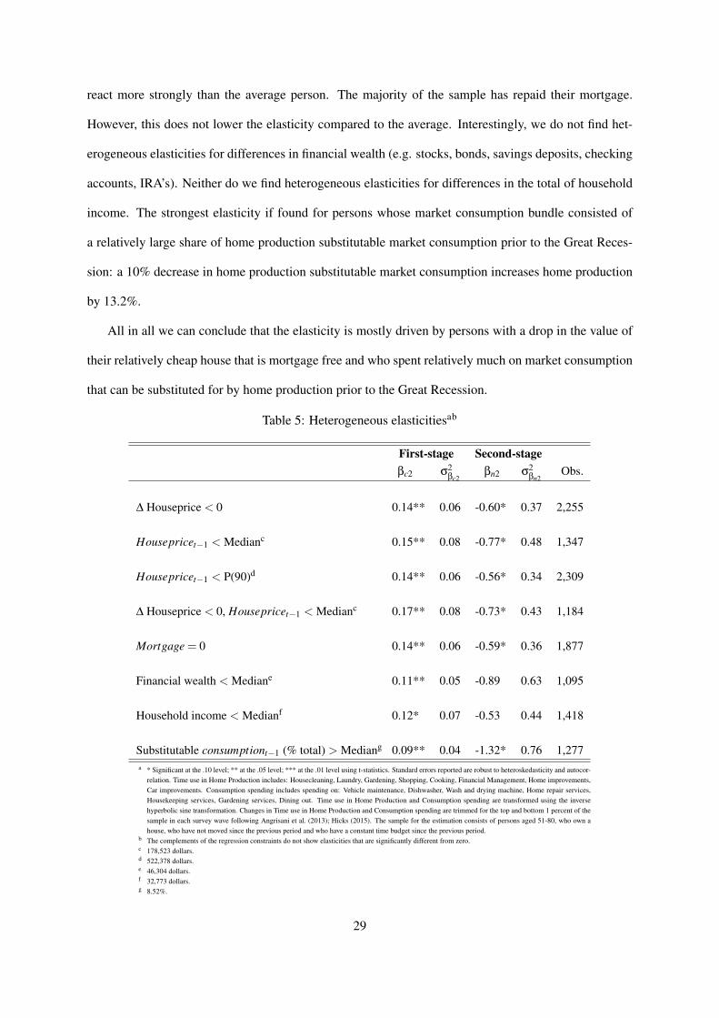
react more strongly than the average person. The majority of the sample has repaid their mortgage.

However, this does not lower the elasticity compared to the average. Interestingly, we do not find het-

erogeneous elasticities for differences in financial wealth (e.g. stocks, bonds, savings deposits, checking

accounts, IRA’s). Neither do we find heterogeneous elasticities for differences in the total of household

income. The strongest elasticity if found for persons whose market consumption bundle consisted of

a relatively large share of home production substitutable market consumption prior to the Great Reces-

sion: a 10% decrease in home production substitutable market consumption increases home production

by 13.2%.

All in all we can conclude that the elasticity is mostly driven by persons with a drop in the value of

their relatively cheap house that is mortgage free and who spent relatively much on market consumption

that can be substituted for by home production prior to the Great Recession.

Table 5: Heterogeneous elasticitiesab

First-stage Second-stageβc2 σ2

βc2βn2 σ2

βn2Obs.

∆ Houseprice < 0 0.14** 0.06 -0.60* 0.37 2,255

Housepricet−1 < Medianc 0.15** 0.08 -0.77* 0.48 1,347

Housepricet−1 < P(90)d 0.14** 0.06 -0.56* 0.34 2,309

∆ Houseprice < 0, Housepricet−1 < Medianc 0.17** 0.08 -0.73* 0.43 1,184

Mortgage = 0 0.14** 0.06 -0.59* 0.36 1,877

Financial wealth < Mediane 0.11** 0.05 -0.89 0.63 1,095

Household income < Medianf 0.12* 0.07 -0.53 0.44 1,418

Substitutable consumptiont−1 (% total) > Mediang 0.09** 0.04 -1.32* 0.76 1,277a * Significant at the .10 level; ** at the .05 level; *** at the .01 level using t-statistics. Standard errors reported are robust to heteroskedasticity and autocor-

relation. Time use in Home Production includes: Housecleaning, Laundry, Gardening, Shopping, Cooking, Financial Management, Home improvements,Car improvements. Consumption spending includes spending on: Vehicle maintenance, Dishwasher, Wash and drying machine, Home repair services,Housekeeping services, Gardening services, Dining out. Time use in Home Production and Consumption spending are transformed using the inversehyperbolic sine transformation. Changes in Time use in Home Production and Consumption spending are trimmed for the top and bottom 1 percent of thesample in each survey wave following Angrisani et al. (2013); Hicks (2015). The sample for the estimation consists of persons aged 51-80, who own ahouse, who have not moved since the previous period and who have a constant time budget since the previous period.

b The complements of the regression constraints do not show elasticities that are significantly different from zero.c 178,523 dollars.d 522,378 dollars.e 46,304 dollars.f 32,773 dollars.g 8.52%.

29

8 Conclusion

The theory of home production suggests that people will substitute away from market consumption as

the opportunity cost of time drops (Becker, 1965). Shifting away from market consumption to home pro-

duction makes people able to smooth consumption in response to income decreases (Hicks, 2015). This

is relevant as home production might be used to mitigate the consequences of shocks in unemployment,

health, retirement and wealth for well-being.

Prior studies have found that people respond to shocks in unemployment (Aguiar et al., 2013), health

(Gimenez-Nadal & Ortega-Lapiedra, 2013), retirement (Aguiar & Hurst, 2005) or wealth (Kuehn, 2015)

by increasing their home production. Hence, people substitute market consumption for home production

as the opportunity cost of time drops. The shocks causing a drop in the opportunity cost of time (re-

tirement, unemployment, disability) have two simultaneous effects 1) it decreases the monetary budget

and 2) it increases the time budget. Therefore, the extent to which home production is a substitute to

market consumption remains unclear as the increases in home production might be due to considerable

increases non-work time available.

Compared to these prior studies, the current paper estimates the intratemporal elasticity between

home production and consumption spending. This elasticity would be a direct measure of the degree of

substitution between home production and market consumption. To exclude possible effects of a chang-

ing time budget we estimate an IV-GMM model in which consumption spending is instrumented with a

wealth shock. A wealth shock is likely to decrease the monetary budget and therefore market consump-

tion (instrument relevance), but is unrelated to the time budget (instrument validity). More specifically,

we use the large and unanticipated shock in houseprices during the Great Recession (Christelis et al.,

2015; Angrisani et al., 2013; Kuehn, 2015) to identify the estimation of the elasticity. To exclude any

possible effects of the Great Recession on the non-market time available, we estimate elasticities for

retirees only.

We find that a 10% decrease in market consumption that can be substituted for by home produc-

tion increases the time spent in home production activities by about 6.5%. The elasticity implies that

a part of the decreased market consumption possibilities can be replaced by home production to miti-

30

gate the consequences of wealth shocks for well-being. The scope for doing so remains rather limited,

however. Home production substitutable market consumption makes up 12% of total consumption, on

average, which makes it small but non-negligible. The other 88% of total consumption, on average, can

not be substituted by home production. The elasticity is mostly driven by persons with a drop in the

value of their relatively cheap home that is free of mortgage and who spent relatively much on market

consumption that can be substituted for by home production prior to the Great Recession.

Our findings suggest that much of the home production responses to shocks in income found by

earlier studies are likely to be the consequence of increased total time available for home production.

Hence, the elasticity between home production and non-market time available is likely to be bigger than

the elasticity between home production and market consumption. Moreover, our results are in contrast

with the typically assumed high substitutability between market consumption and home production in

existing theoretical models (Campbell & Ludvigson, 2001). Nonetheless, it should be kept in mind that

our results are identified by a sample of retirees. Responses of prime age workers may be different as

their opportunity costs of home production are likely to be different.

References

Aguiar, M., & Hurst, E. (2005). Consumption versus expenditure. Journal of Political Economy, 113(5),919–948.

Aguiar, M., Hurst, E., & Karabarbounis, L. (2012). Recent developments in the economics of time use.Annual Review of Economics, 4, 373–397.

Aguiar, M., Hurst, E., & Karabarbounis, L. (2013). Time use during the Great Recession. AmericanEconomic Review, 103, 1664–1696.

Aguila, E., Attanasio, O., & Meghir, C. (2011). Changes in consumption at retirement: Evidence frompanel data. Review of Economics and Statistics, 3, 1094–1099.

Ahn, N., Jimeno, J., & Ugidos, A. (2008). ”Mondays at the sun”: Unemployment, time-use, andconsumption patterns in Spain. (FEDEA Working Paper Paper, No. 2003-18)

Alessie, R., & De Ree, J. (2008). Home production and the allocation of time and consumption over thelife cycle. (Netspar Discussion Paper, No. 2008-020)

Angrisani, M., Hurd, M., & Rohwedder, S. (2013). Changes in spending in the Great Recessionfollowing stock and housing wealth losses. (mimeo)

31

Apps, P., & Rees, R. (1997). Collective labour supply and household production. Journal of PoliticalEconomy, 105, 178–190.

Apps, P., & Rees, R. (2005). Gender, time use, and public policy over the life-cycle. Oxford Review ofEconomic Policy, 21, 439–461.

Banks, J., Blundell, R., & Tanner, S. (1998). Is there a retirement-savings puzzle? American EconomicReview, 88(4), 769–788.

Battistin, E., Brugiavini, A., Rettore, E., & Weber, G. (2009). The retirement consumption puzzle:Evidence from a regression discontinuity approach. American Economic Review, 99, 2209–2226.

Baxter, M., & Jermann, U. (1999). Household productivity and the excess sensitivity of consumption tocurrent income. American Economic Review, 89, 902–920.

Becker, G. (1965). A theory of the allocation of time. The Economic Journal, 75, 493–517.

Benhabib, J., Rogerson, R., & Wright, R. (1991). Homework in macroeconomics: Household produc-tion and aggregate fluctuations. Journal of Political Economy, 99, 1166–1187.

Bernheim, B., Skinner, J., & Weinberg, S. (2001). What accounts for the variation in retirement wealthamong US households? American Economic Review, 91(4), 832–857.

Burda, M., & Hamermesh, D. (2010). Unemployment, market work and household production. Eco-nomics Letters, 107, 131–133.

Campbell, J., & Cocco, J. (2007). How do house prices affect consumption? Evidence from micro data.Journal of Monetary Economics, 54, 591–621.

Campbell, J., & Ludvigson, S. (2001). Elasticities of substitution in Real Business Cycle models withhome production. Journal of Money, Credit, and Banking, 33, 847–875.

Christelis, D., Georgarakos, D., & Jappelli, T. (2015). Wealth shocks, unemployment shocks andconsumption in the wake of the Great Recession. Journal of Monetary Economics, 72, 21–41.

Colella, F., & Van Soest, A. (2013). Time use, consumption expenditures and employment status:Evidence from the LISS panel. (Paper presented at the 7th MESS Workshop)

Deaton, A. (1971). Wealth effects on consumption in a modified life-cycle model. Review of EconomicStudies, 39(4), 443–453.

Dotsey, M., Li, W., & Yang, F. (2010). Consumption and time use over the life-cycle. (Federal ReserveBank of Philadelphia Research Department Working Paper, No. 10-37)

Fang, L., & Zhu, G. (2012). Home production technology and time allocation - empirics, theory andimplications. (mimeo)

Ghez, G., & Becker, G. (1975). The allocation of time and goods over the life cycle. New York:Columbia University Press.

32

Gimenez-Nadal, J., & Ortega-Lapiedra, R. (2013). Health status and time allocation in spain. AppliedEconomics Letters, 20(15), 1435–1439.

Gortz, M. (2006). Heterogeneity in preferences and productivity - implications for retirement. (Leisure,household production, consumption and economic well-being, Ph.D. thesis, Chapter 4)

Greenwood, J., & Hercowitz, Z. (1991). The allocation of capital and time over the business cycle.Journal of Political Economy, 99, 1188–1214.

Greenwood, J., Rogerson, R., & Wright, R. (1995). Household production in Real Business Cycletheory. In T. Cooley (Ed.), Frotniers of Business Cycle research (p. 157-174). Princeton: PrincetonUniversity Press.

Griffith, R., O’Connell, M., & Smith, K. (2014). Shopping around? How households adjusted foodspending over the Great Recession. (paper presented at the EEA-ESEM 2014, Toulouse)

Gronau, R. (1977). Leisure, home production and work - the theory of the allocation of time revisited.Journal of Political Economy, 85, 1099–1124.

Guler, B., & Taskin, T. (2013). Does unemployment insurance crowd out home production? EuropeanEconomic Review, 62, 1–16.

Hall, R. (2009). Reconciling cyclical movements in the marginal value of time and the marginal productof labor. Journal of Political Economy, 117, 281–323.

Halliday, T., & Podor, M. (2012). Health status and the allocation of time. Health Economics, 21,514–527.

Hicks, D. (2015). Consumption volatility, marketization, and expenditure in an emerging market econ-omy. American Economic Journal: Macroeconomics, 7(2), 95–123.

Hurd, M., & Rohwedder, S. (2007). Time-use in the older population. variation by socio-economicstatus and health. (RAND Labor and Population Working Paper Series, No. WP-463)

Hurd, M., & Rohwedder, S. (2008). The adequacy of economic resources in retirement. (MRRCWorking Paper Series, No. WP2008-184)

Hurd, M., & Rohwedder, S. (2009). Methodological innovations in collecting spending data: The HRSConsumption and Activities Mail Survey. Fiscal Studies, 30(3/4), 435–459.

Hurd, M., & Rohwedder, S. (2013). Heterogeneity in spending change at retirement. The Journal of theEconomics of Aging, 1-2, 60–71.

Hurst, E. (2008). The retirement of a consumption puzzle. (NBER Working Paper Series, No. 13789)

Kalwij, A., & Alessie, R. (2007). Permanent and transitory wages of British men, 1975-2001: Year, ageand cohort effects. Journal of Applied Econometrics, 22, 1063–1093.

33

Karabarbounis, L. (2014). Home production, labor wedges, and international business cycles. Journalof Monetary Economics, 64, 68–84.

Krueger, A., & Mueller, A. (2012). Time use, emotional well-being, and unemployment: Evidence fromlongitudinal data. American Economic Review: Papers & Proceedings, 102, 594–599.

Kuehn, D. (2015). Home production, house values, and the great recession. Journal of Family andEconomic Issues, DOI 10.1007/s10834-015-9438-3.

Laitner, J., & Silverman, D. (2005). Estimating life-cycle parameters from consumption behavior atretirement. (NBER Working Paper Series, No. 11163)

Mariger, R. (1987). A life-cycle consumption model with liquidity constraints: Theory and empiricalresults. Econometrica, 55, 533–557.

Miniaci, R., Monfardini, C., & Weber, G. (2003). Is there a retirement-consumption puzzle in Italy?(Institute for Fiscal Studies Working Paper Series, No. 03/14)

Parker, J. (1999). The reaction of household consumption to predictable changes in social security taxes.American Economic Review, 89, 959–973.

Robb, A., & Burbidge, J. (1989). Consumption, income, and retirement. Canadian Journal of Eco-nomics, 22, 522–542.

Rogerson, R., & Wallenius, J. (2013). Nonconvexities, retirement, and the elasticity of labor supply.American Economic Review, 103, 1445–1462.

Rupert, P., Rogerson, R., & Wright, R. (1995). Estimating substitution elasticities in household produc-tion models. Economic Theory, 6, 179–193.

Rupert, P., Rogerson, R., & Wright, R. (2000). Homework in labor economics: Household productionand intertemporal substitution. Journal of Monetary Economics, 46, 557–579.

Stancanelli, E., & Van Soest, A. (2012). Retirement and home production: A regression discontinuityapproach. American Economic Review, 102(2), 600–605.

Taskin, T. (2011). Unemployment insurance and home production. (MPRA Working Paper, No. 34878)

Velarde, M., & Herrmann, R. (2014). How retirement changes consumption and household productionof food: Lessons from German time-use data. The Journal of the Economics of Aging, 3, 1–10.

34