Embed Size (px)
Citation preview
econstorMake Your Publications Visible.
A Service of
zbwLeibniz-InformationszentrumWirtschaftLeibniz Information Centrefor Economics
Wagner, Regina; Blecker, Thorsten
Conference Paper
Material Requirements Planning under Phase-outConditions
Provided in Cooperation with:Hamburg University of Technology (TUHH), Institute of Business Logistics and GeneralManagement
Suggested Citation: Wagner, Regina; Blecker, Thorsten (2015) : Material RequirementsPlanning under Phase-out Conditions, In: Blecker, Thorsten Kersten, Wolfgang Ringle, ChristianM. (Ed.): Operational Excellence in Logistics and Supply Chains: Optimization Methods, Data-driven Approaches and Security Insights. Proceedings of the Hamburg International Conferenceof Logistics (HICL), Vol. 22, ISBN 978-3-7375-4058-2, epubli GmbH, Berlin, pp. 73-95
This Version is available at:http://hdl.handle.net/10419/209282
Standard-Nutzungsbedingungen:
Die Dokumente auf EconStor dürfen zu eigenen wissenschaftlichenZwecken und zum Privatgebrauch gespeichert und kopiert werden.
Sie dürfen die Dokumente nicht für öffentliche oder kommerzielleZwecke vervielfältigen, öffentlich ausstellen, öffentlich zugänglichmachen, vertreiben oder anderweitig nutzen.
Sofern die Verfasser die Dokumente unter Open-Content-Lizenzen(insbesondere CC-Lizenzen) zur Verfügung gestellt haben sollten,gelten abweichend von diesen Nutzungsbedingungen die in der dortgenannten Lizenz gewährten Nutzungsrechte.
Terms of use:
Documents in EconStor may be saved and copied for yourpersonal and scholarly purposes.
You are not to copy documents for public or commercialpurposes, to exhibit the documents publicly, to make thempublicly available on the internet, or to distribute or otherwiseuse the documents in public.
If the documents have been made available under an OpenContent Licence (especially Creative Commons Licences), youmay exercise further usage rights as specified in the indicatedlicence.
https://creativecommons.org/licenses/by-sa/4.0/
www.econstor.eu
Proceedings of the Hamburg Inter
Regina Wagner and Thorsten Blecker
Material Requirementsunder Phase out Condiunder Phase-out Condi
Published in: Operational Excellence in Logistics and Su
Thorsten Blecker, Wolfgang Kersten and Christian M. Ri
ISBN (online): 978-3-7375-4058-2, ISBN (print): 978-3-737
ISSN (online): 2365-5070, ISSN (print): 2635-4430
rnational Conference of Logistics (HICL) – 22
s Planning tionstions
pply Chains
ngle (Eds.), August 2015, epubli GmbH
75-4056-8
Material Requirements Planning under Phase-out Conditions
Regina Wagner and Thorsten Blecker
In today’s production environment with shortened product lifecycles, phase-outs, i.e. product elimination from production, become regular events. Badly planned phase-outs lead to high remaining stock levels after end of production, causing im-mense sunk costs. Previously performed 26 interviews revealed that this is a major challenge in current production (Grussenmeyer and Blecker, 2014; Grussenmeyer, Gencay and Blecker, 2014). Therefore, the objective of this paper is to develop a ma-terial requirements planning focusing on remaining stock induced costs during phase-out to plan optimal phase-out quantity and phase-out date. The research is conceptually driven and proposes an example of the methodology.
Keywords: Phase-Out, Product Elimination, Production Planning and Control, Remaining Stock Costs
74 Regina Wagner and Thorsten Blecker
1 Introduction
Shortened product life cycles are significant current trends of supply net-
works (Bakker, Wang, Huisman and den Hollander, 2014, p.10). They lead
to frequent product changes in order to satisfy customer’s demand
(Slamanig, 2011, p.46).
Enabling successful product’s ramp-ups requires production capacities
availability. Since 80% of the new products are symmetrical replacements
(Saunders and Jobber, 1988), companies use the old generation’s produc-
tion plant as well for the replacement’s manufacturing, implying an equip-
ment change. Thus, the old product needs to be eliminated in order to re-
lease the demanded production capacity (Vyas, 1993, p.68). Product elimi-
nation implementations mostly are realized as phase-outs (Avlonitis, 1983;
Mitchell, Taylor and Tanyel, 1998; Baker and Hart, 2007), and their success
depends on phase-out’s process quality (Prigge, 2008). The need of having
good phase-out processes is also described by practitioners (Holzhäuer
and Riepl, 1996, p.49). Still, very few research deals with phase-out and its
processes.
Phase-out can be described in a four-stage process, starting after product
elimination decision-making. The two main stages are planning and imple-
mentation, framed by definition and finalization, describing the actual
dealing with phase-out in the production department.
To successfully produce products, and therefore, as well to phase-out prod-
ucts, companies use production planning and control (PPC). Adopting this,
especially the material requirements planning is a key issue in phase-out
planning for not having any remaining stock after end of production
Material Requirements Planning under Phase-out Conditions 75
(Holtsch, 2009; Hertrampf, 2012). To appropriately plan material require-
ments, this publication presents a methodology to estimate remaining
stock costs.
The outline of this publication is as follows. After reviewing literature in
chapter 2, equations to calculate remaining stock costs are elaborated in
chapter 3. The following chapter 4 presents a phase-out example to
demonstrate the methodology’s functionalities. Chapter 5 summarizes the
results.
2 Literature Review
Eliminating products from the company’s portfolio is considered as an un-
inspiring and depressing task (Eckles, 1971, p.72) Nevertheless, in today’s
competitive environment, it is becoming more and more important (Prigge,
2008, p.100). After elimination decision-making, the implementation strat-
egy needs to be determined (Avlonitis, Hart and Tzokas, 2000, p.54). From
marketing point of view, five options are available, namely drop immedi-
ately, phase-out immediately, phase-out slowly, sell-out and drop from
standard and re-introduce as special strategies (Baker and Hart, 2007,
p.478).
2.1 Product Phase-Out
From a production point of view, only the phase-out strategies are interest-
ing to investigate due to several reasons. The drop immediately strategy
implies a direct machine stop, without any potential for improvement. The
sell-out and drop strategy only induce marketing activities. In cases of plant
76 Regina Wagner and Thorsten Blecker
sale, production does not change, while when product’s rights are sold by
ending production, a phase-out takes place. The situation is similar to the
drop strategy. Even though the product might be re-introduced as a special
after its normal end of production, it necessarily has to be phased-out be-
fore. Thus, this paper deals with the planned phase-out of a product.
In literature, product phase-out definitions are not clear. Apart from the
fact that many authors use the term without defining it before (e.g. Inness,
1994; Holzhäuer and Riepl, 1996; Aurich, Naab and Barbian, 2005; Kotler
and Armstrong, 2010) other definitions only include the production reduc-
tion from full capacity run to end of production (e.g. Kirsch and Buchholz,
2008; Ostertag, 2008; Scholz-Reiter, Baumbach and Krohne, 2008; Elbert,
2011) without considering any planning. Therefore, we define the product
phase-out as “process, enabling companies to eliminate a product. The
phase-out is subsequent to the phase-out decision and starts with the plan-
ning. The phase-out ends with the finalization after the end of production”
(adopted from Grussenmeyer and Blecker, 2014, p.185).
Several authors assume a correlation between the market’s decline phase
and product phase-out (e.g. Aurich and Naab, 2006; Hertrampf, Nickel and
Nyhuis, 2010) even though Avlonitis (1990, pp.55–60) detected that prod-
ucts are eliminated irrespective of their position in the product life cycle.
Consequently, a phase-out may also take place at any time during the prod-
uct’s life.
2.2 Planning and Controlling Product Phase-Outs
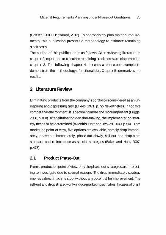
Holtsch (2009, pp.54–60) described that previous publications do not deal
with phase-out PPC. He then developed an 8-phase phase-out reference
Material Requirements Planning under Phase-out Conditions 77
process intending to give industry a guideline to plan and control phase-
out (Figure 1).
Figure 1 Phase-out Control Process; Source: Holtsch (2009, p.62)
The phase-out PPC process presented by Holtsch is limited to phase-out
induced remaining stock costs without referring to any further phase-out
aspects. In addition, he does not follow any of the existing PPC models (e.g.
Hornung, 1996; Hackstein, 1989; Lödding, 2005; Schuh, 2006) which he an-
alyzed in his work. Holtsch (2009, p.111) only adds four activities to produc-
tion plan generation and one function to make-or-buy decision-making to
the Aachener PPS Modell (Aachen PPC Model Hornung 1996).
In his first process stage – phase-out decision-making – he aggregates re-
quirements of different stakeholders without giving any elimination deci-
sion-making model on how to decide to phase-out, and without referring
to any product elimination literature. For the second process stage – com-
ponent identification – he develops a phase-out cube, with the three di-
mensions (ranging from N via O to P) phase-out coefficient, normative
range of stock and normative stock value (as described in Holtsch (2009,
p.74)). The cube’s axes seem to have different relevance (e.g. NPO = neutral
/ OPN = dispositive adoption / PNO = phase-out relevant), where the phase-
out coefficient is the main influence factor, but no justification is given.
Phase-out decision Identification of relevant components
Calculation of expected remaining
stock costs depending on phase-out day
Definition of phase-out day (incl. costs
and other limitations)
Definition of adequate means for the cost
reductionDefinition of final
activities cataloguePhase-out steeringDocumentation
78 Regina Wagner and Thorsten Blecker
The third process stage is to calculate the expected remaining stock costs
(inventory multiplied by unit costs) for all product components. This for-
mula does not include multi-variant phase-outs where there might not only
be one optimum phase-out day. At this stage, only unit costs are consid-
ered, i.e. remaining stock handling costs are entirely neglected. Further-
more, the amount of items or parts expected to become remaining stock is
considered as input variable, obliging the companies themselves to de-
velop calculation models. Process stages four and five summate all part’s
costs during phase-out (inventory costs, remaining stock costs, process
costs, as well as income or losses from remaining stocks options) in addi-
tion to general phase-out management costs. In the sixths process stage,
all options are then balanced to obtain the maximum profit. Process stage
seven, i.e. phase-out control, is described as standard control loop without
detailing any methodologies applicable. The author also describes how to
perform multi phase-outs (subsequent or parallel) by adopting the control
loop, but he does not include multi phase-outs into his planning process
(Holtsch, 2009, pp.61–109). Therefore, it is necessary to develop a phase-
out PPC model complying with specific phase-out objectives.
To close the first part of this gap, a methodology how to really calculate the
expected remaining stock at end of production and its induced costs is pre-
sented in the following chapter.
3 Expected Remaining Stock
Material requirements planning can follow stochastic, deterministic and
heuristic approaches. In general, stochastic models are applied for high
Material Requirements Planning under Phase-out Conditions 79
volume, low cost products, while deterministic models are used for high
costs, low volume products. New products or products with unknown de-
mand are calculated with heuristic models; which are therefore not rele-
vant for phase-out. All models include decisions on production and inven-
tory quantities and the identification of relevant costs, e.g. variable produc-
tion costs, setup costs, and inventory costs. Similar to standard production
planning, a phase-out plan is created in a rolling horizon fashion, to be up-
dated after implementing the first decisions. The revised plan minimizes
demand forecast and production uncertainties (Graves, 2001, p.730). Pro-
duction planning figures are non-negative integers (∈ℕ0).
The first planning step is to determine the amount of lots for every part j to
be purchased during phase-out for producing all phase-out items i follow-
ing the standard deterministic approach. The result then needs to be com-
pared to existing contract limitations, e.g. lot sizes, which lacks in existing
literature. For example. Hertrampf (2012) only reduces lot sizes by incorpo-
rating risk costs and Holtsch (2009) does not consider lot size limitations.
80 Regina Wagner and Thorsten Blecker
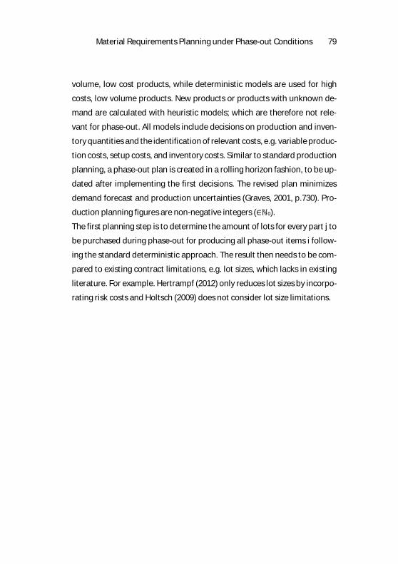
𝑎𝑎𝑎𝑎𝑎𝑎𝑗𝑗𝑗𝑗 =
⎩⎨
⎧�∑ 𝑎𝑎𝑟𝑟𝑖𝑖𝑗𝑗 ∙ �
𝑛𝑛𝑖𝑖𝑗𝑗𝑎𝑎𝐿𝐿𝑖𝑖𝑗𝑗
�𝐼𝐼𝑖𝑖=1 ∙ 𝑎𝑎𝐿𝐿𝑖𝑖𝑗𝑗 − 𝑠𝑠𝑗𝑗𝑗𝑗−1 + 𝑠𝑠𝑠𝑠𝑗𝑗𝑗𝑗
𝑎𝑎𝑎𝑎𝐿𝐿𝑗𝑗𝑗𝑗� 𝑖𝑖𝑖𝑖 𝑛𝑛𝑖𝑖𝑗𝑗 > 0
0 𝑒𝑒𝑒𝑒𝑠𝑠𝑒𝑒
(1)
𝑎𝑎𝑟𝑟𝑖𝑖𝑗𝑗 ,𝑎𝑎𝑎𝑎𝐿𝐿𝑗𝑗𝑗𝑗 > 0
∀𝑖𝑖 ∈ 𝐼𝐼, 𝑗𝑗 ∈ 𝐽𝐽, 𝑡𝑡 ∈ 𝑇𝑇
aoit amount of items i ordered in period t [pcs]
aPLjt amount of procurement lots of part j in period t [u/m]
arij amount of part j required for item i [pcs/pcs]
LSit production lot size of item i in period t [pcs/(u/m)]
nit need of item i in period t [pcs], i.e. 𝑎𝑎𝑎𝑎𝑖𝑖𝑗𝑗 − 𝑠𝑠𝑖𝑖𝑗𝑗−1 [pcs]
PLSjt procurement lot size of part j in period t [pcs/(u/m)]
Qj(τ) repair parts order quantity [pcs]
spjt spare parts need of part j in period t [pcs] (equation (2))
sit-1 stock of item i at the beginning of period t [pcs]
sjt-1 stock of part j at the beginning of period t [pcs]
subject to 𝑄𝑄𝑗𝑗(𝜏𝜏) = �𝑠𝑠𝑠𝑠𝑗𝑗𝑗𝑗
𝑇𝑇
𝑗𝑗=1
∀𝑗𝑗 ∈ 𝐽𝐽 (2)
To determine the spare parts order quantity 𝑄𝑄𝑗𝑗(𝜏𝜏) and the spare parts need
spjt, please consult the publication of Sahyouni et al (2010, p.794) who pre-
sent a deterministic optimization model.
Material Requirements Planning under Phase-out Conditions 81
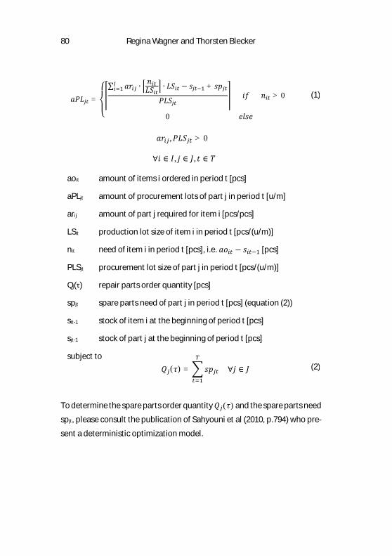
Equation (1) calculates the ceiling of the necessary procurement lots of
part j, i.e. the smallest integer greater or equal to the equation. The equa-
tion combines information of the quantity bill of materials with the existing
demand subtracted by items i on stock. The division by the procurement
lot size directly links the calculated need to procurement limitations. It is
necessary to summate over all items i to obtain the parts’ need for all
phase-out items. For any situation where the amount of orders can already
be covered by the stock on hand, the procurement lot size decreases to
zero. Multiplying the amount of procurement lots with the lot size gives the
stock level of part j, as given in equation (3).
𝑠𝑠𝑗𝑗𝑗𝑗 = 𝑎𝑎𝑎𝑎𝑎𝑎𝑗𝑗𝑗𝑗 ∙ 𝑎𝑎𝑎𝑎𝐿𝐿𝑗𝑗𝑗𝑗 + 𝑠𝑠𝑗𝑗𝑗𝑗−1 ∀𝑗𝑗 ∈ 𝐽𝐽, 𝑡𝑡 ∈ 𝑇𝑇 (3)
aPLjt amount of procurement lots of part j in period t [u/m] (eq. (1))
PLSjt procurement lot size of part j in period t [pcs/(u/m)]
sjt stock of part j at end of period t [pcs]
sjt-1 stock of part j at the beginning of period t [pcs]
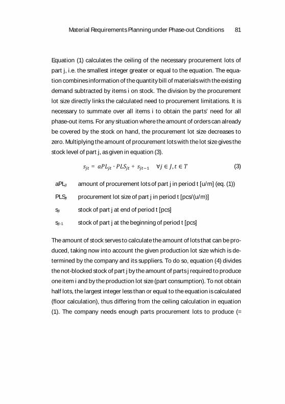
The amount of stock serves to calculate the amount of lots that can be pro-
duced, taking now into account the given production lot size which is de-
termined by the company and its suppliers. To do so, equation (4) divides
the not-blocked stock of part j by the amount of parts j required to produce
one item i and by the production lot size (part consumption). To not obtain
half lots, the largest integer less than or equal to the equation is calculated
(floor calculation), thus differing from the ceiling calculation in equation
(1). The company needs enough parts procurement lots to produce (=
82 Regina Wagner and Thorsten Blecker
rounding up), leading to a limited amount of item’s production lots (=
rounding).
𝑎𝑎𝑎𝑎𝑖𝑖𝑗𝑗𝑗𝑗 = �𝑠𝑠𝑗𝑗𝑗𝑗 − 𝑠𝑠𝑠𝑠𝑗𝑗𝑗𝑗𝑎𝑎𝐿𝐿𝑖𝑖𝑗𝑗 ∙ 𝑎𝑎𝑟𝑟𝑖𝑖𝑗𝑗
� ∀𝑖𝑖 ∈ 𝐼𝐼, 𝑗𝑗 ∈ 𝐽𝐽, 𝑡𝑡 ∈ 𝑇𝑇 (4)
𝑎𝑎𝑟𝑟𝑖𝑖𝑗𝑗 ,𝑎𝑎𝐿𝐿𝑖𝑖𝑗𝑗 > 0 ∀𝑖𝑖 ∈ 𝐼𝐼, 𝑗𝑗 ∈ 𝐽𝐽, 𝑡𝑡 ∈ 𝑇𝑇
aLijt amount of production lots of item i in period t with given part j [u/m]
arij amount of part j required for item i [pcs/pcs]
LSit production lot size of item i in period t [pcs/(u/m)]
sjt stock of part j at end of period t [pcs] (eq. (3))
spjt spare parts need of part j in period t [pcs] (eq. (2))
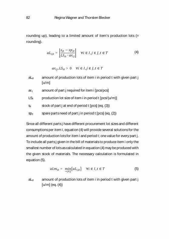
Since all different parts j have different procurement lot sizes and different
consumptions per item i, equation (4) will provide several solutions for the
amount of production lots for item i and period t; one value for every part j.
To include all parts j given in the bill of materials to produce item i only the
smallest number of lots as calculated in equation (4) may be produced with
the given stock of materials. The necessary calculation is formulated in
equation (5).
𝑎𝑎𝑎𝑎𝑎𝑎𝑖𝑖𝑗𝑗 = 𝑎𝑎𝑖𝑖𝑛𝑛→𝑗𝑗∈𝐽𝐽
�𝑎𝑎𝑎𝑎𝑖𝑖𝑗𝑗𝑗𝑗� ∀𝑖𝑖 ∈ 𝐼𝐼, 𝑡𝑡 ∈ 𝑇𝑇 (5)
aLijt amount of production lots of item i in period t with given part j [u/m] (eq. (4))
Material Requirements Planning under Phase-out Conditions 83
aLmit minimum amount of production lots for item i in period t [u/m]
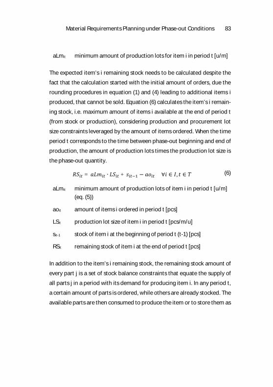
The expected item’s i remaining stock needs to be calculated despite the
fact that the calculation started with the initial amount of orders, due the
rounding procedures in equation (1) and (4) leading to additional items i
produced, that cannot be sold. Equation (6) calculates the item’s i remain-
ing stock, i.e. maximum amount of items i available at the end of period t
(from stock or production), considering production and procurement lot
size constraints leveraged by the amount of items ordered. When the time
period t corresponds to the time between phase-out beginning and end of
production, the amount of production lots times the production lot size is
the phase-out quantity.
𝑅𝑅𝐿𝐿𝑖𝑖𝑗𝑗 = 𝑎𝑎𝑎𝑎𝑎𝑎𝑖𝑖𝑗𝑗 ∙ 𝑎𝑎𝐿𝐿𝑖𝑖𝑗𝑗 + 𝑠𝑠𝑖𝑖𝑗𝑗−1 − 𝑎𝑎𝑎𝑎𝑖𝑖𝑗𝑗 ∀𝑖𝑖 ∈ 𝐼𝐼, 𝑡𝑡 ∈ 𝑇𝑇 (6)
aLmit minimum amount of production lots of item i in period t [u/m] (eq. (5))
aoit amount of items i ordered in period t [pcs]
LSit production lot size of item i in period t [pcs/m/u]
sit-1 stock of item i at the beginning of period t (t-1) [pcs]
RSit remaining stock of item i at the end of period t [pcs]
In addition to the item’s i remaining stock, the remaining stock amount of
every part j is a set of stock balance constraints that equate the supply of
all parts j in a period with its demand for producing item i. In any period t,
a certain amount of parts is ordered, while others are already stocked. The
available parts are then consumed to produce the item or to store them as
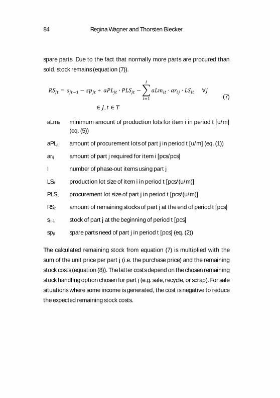
84 Regina Wagner and Thorsten Blecker
spare parts. Due to the fact that normally more parts are procured than
sold, stock remains (equation (7)).
𝑅𝑅𝐿𝐿𝑗𝑗𝑗𝑗 = 𝑠𝑠𝑗𝑗𝑗𝑗−1 − 𝑠𝑠𝑠𝑠𝑗𝑗𝑗𝑗 + 𝑎𝑎𝑎𝑎𝑎𝑎𝑗𝑗𝑗𝑗 ∙ 𝑎𝑎𝑎𝑎𝐿𝐿𝑗𝑗𝑗𝑗 −�𝑎𝑎𝑎𝑎𝑎𝑎𝑖𝑖𝑗𝑗 ∙ 𝑎𝑎𝑟𝑟𝑖𝑖𝑗𝑗 ∙ 𝑎𝑎𝐿𝐿𝑖𝑖𝑗𝑗
𝐼𝐼
𝑖𝑖=1
∀𝑗𝑗
∈ 𝐽𝐽, 𝑡𝑡 ∈ 𝑇𝑇
(7)
aLmit minimum amount of production lots for item i in period t [u/m] (eq. (5))
aPLjt amount of procurement lots of part j in period t [u/m] (eq. (1))
arij amount of part j required for item i [pcs/pcs]
I number of phase-out items using part j
LSit production lot size of item i in period t [pcs/(u/m)]
PLSjt procurement lot size of part j in period t [pcs/(u/m)]
RSjt amount of remaining stocks of part j at the end of period t [pcs]
sjt-1 stock of part j at the beginning of period t [pcs]
spjt spare parts need of part j in period t [pcs] (eq. (2))
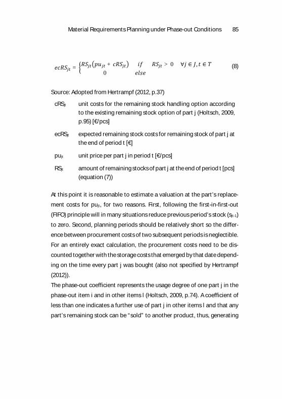
The calculated remaining stock from equation (7) is multiplied with the
sum of the unit price per part j (i.e. the purchase price) and the remaining
stock costs (equation (8)). The latter costs depend on the chosen remaining
stock handling option chosen for part j (e.g. sale, recycle, or scrap). For sale
situations where some income is generated, the cost is negative to reduce
the expected remaining stock costs.
Material Requirements Planning under Phase-out Conditions 85
𝑒𝑒𝑒𝑒𝑅𝑅𝐿𝐿𝑗𝑗𝑗𝑗 = �𝑅𝑅𝐿𝐿𝑗𝑗𝑗𝑗�𝑠𝑠𝑝𝑝𝑗𝑗𝑗𝑗 + 𝑒𝑒𝑅𝑅𝐿𝐿𝑗𝑗𝑗𝑗� 𝑖𝑖𝑖𝑖 𝑅𝑅𝐿𝐿𝑗𝑗𝑗𝑗 > 0 ∀𝑗𝑗 ∈ 𝐽𝐽, 𝑡𝑡 ∈ 𝑇𝑇0 𝑒𝑒𝑒𝑒𝑠𝑠𝑒𝑒
(8)
Source: Adopted from Hertrampf (2012, p.37)
cRSjt unit costs for the remaining stock handling option according to the existing remaining stock option of part j (Holtsch, 2009, p.95) [€/pcs]
ecRSjt expected remaining stock costs for remaining stock of part j at the end of period t [€]
pujt unit price per part j in period t [€/pcs]
RSjt amount of remaining stocks of part j at the end of period t [pcs] (equation (7))
At this point it is reasonable to estimate a valuation at the part’s replace-
ment costs for pujt, for two reasons. First, following the first-in-first-out
(FIFO) principle will in many situations reduce previous period’s stock (sjt-1)
to zero. Second, planning periods should be relatively short so the differ-
ence between procurement costs of two subsequent periods is neglectible.
For an entirely exact calculation, the procurement costs need to be dis-
counted together with the storage costs that emerged by that date depend-
ing on the time every part j was bought (also not specified by Hertrampf
(2012)).
The phase-out coefficient represents the usage degree of one part j in the
phase-out item i and in other items l (Holtsch, 2009, p.74). A coefficient of
less than one indicates a further use of part j in other items l and that any
part’s remaining stock can be “sold” to another product, thus, generating
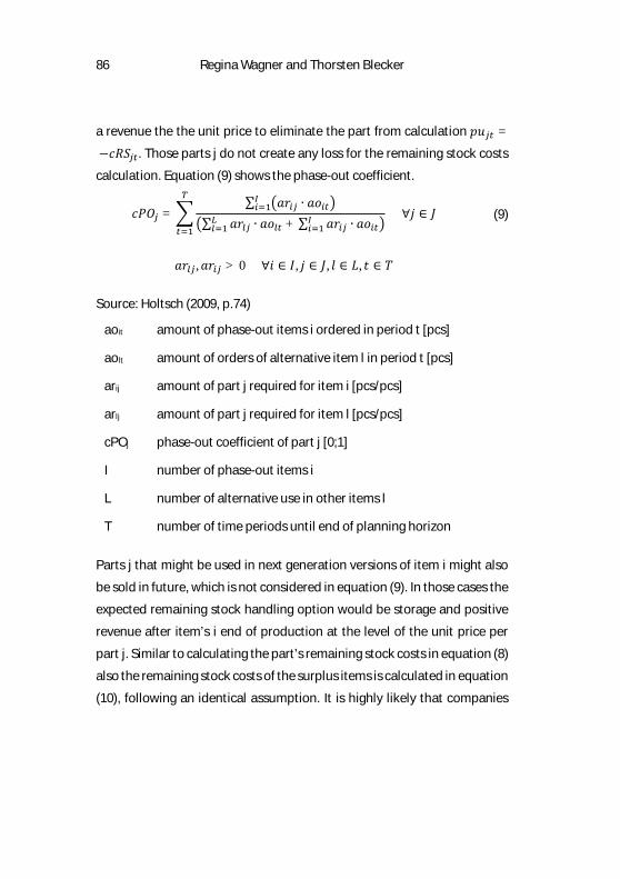
86 Regina Wagner and Thorsten Blecker
a revenue the the unit price to eliminate the part from calculation 𝑠𝑠𝑝𝑝𝑗𝑗𝑗𝑗 = −𝑒𝑒𝑅𝑅𝐿𝐿𝑗𝑗𝑗𝑗. Those parts j do not create any loss for the remaining stock costs
calculation. Equation (9) shows the phase-out coefficient.
𝑒𝑒𝑎𝑎𝑐𝑐𝑗𝑗 = �∑ �𝑎𝑎𝑟𝑟𝑖𝑖𝑗𝑗 ∙ 𝑎𝑎𝑎𝑎𝑖𝑖𝑗𝑗�𝐼𝐼𝑖𝑖=1
�∑ 𝑎𝑎𝑟𝑟𝑙𝑙𝑗𝑗 ∙ 𝑎𝑎𝑎𝑎𝑙𝑙𝑗𝑗 + ∑ 𝑎𝑎𝑟𝑟𝑖𝑖𝑗𝑗 ∙ 𝑎𝑎𝑎𝑎𝑖𝑖𝑗𝑗𝐼𝐼𝑖𝑖=1
𝐿𝐿𝑙𝑙=1 �
𝑇𝑇
𝑗𝑗=1
∀𝑗𝑗 ∈ 𝐽𝐽 (9)
𝑎𝑎𝑟𝑟𝑙𝑙𝑗𝑗 , 𝑎𝑎𝑟𝑟𝑖𝑖𝑗𝑗 > 0 ∀𝑖𝑖 ∈ 𝐼𝐼, 𝑗𝑗 ∈ 𝐽𝐽, 𝑒𝑒 ∈ 𝑎𝑎, 𝑡𝑡 ∈ 𝑇𝑇
Source: Holtsch (2009, p.74)
aoit amount of phase-out items i ordered in period t [pcs]
aolt amount of orders of alternative item l in period t [pcs]
arij amount of part j required for item i [pcs/pcs]
arlj amount of part j required for item l [pcs/pcs]
cPOj phase-out coefficient of part j [0;1]
I number of phase-out items i
L number of alternative use in other items l
T number of time periods until end of planning horizon
Parts j that might be used in next generation versions of item i might also
be sold in future, which is not considered in equation (9). In those cases the
expected remaining stock handling option would be storage and positive
revenue after item’s i end of production at the level of the unit price per
part j. Similar to calculating the part’s remaining stock costs in equation (8)
also the remaining stock costs of the surplus items is calculated in equation
(10), following an identical assumption. It is highly likely that companies
Material Requirements Planning under Phase-out Conditions 87
sell remaining stock to at least obtain a lower-than-normal revenue (i.e.
negative cRSit), such as IBM who in 1998 generated a loss of $1 billion due
to excess PC inventory at their dealers which were sold at low special offer
prices (Bulkeley, 1999).
𝑒𝑒𝑒𝑒𝑅𝑅𝐿𝐿𝑖𝑖𝑗𝑗 = �𝑅𝑅𝐿𝐿𝑖𝑖𝑗𝑗(𝑒𝑒𝑠𝑠𝑖𝑖𝑗𝑗 + 𝑒𝑒𝑅𝑅𝐿𝐿𝑖𝑖𝑗𝑗) 𝑖𝑖𝑖𝑖 𝑅𝑅𝐿𝐿𝑖𝑖𝑗𝑗 > 0 ∀𝑖𝑖 ∈ 𝐼𝐼, 𝑡𝑡 ∈ 𝑇𝑇 0 𝑒𝑒𝑒𝑒𝑠𝑠𝑒𝑒
(10)
Source: Adopted from Hertrampf (2012, p.37)
cpit unit cost of production for item i in period t [€/pcs] (in general: material procurement costs, manufacturing costs and related overhead)
cRSit unit costs for the remaining stock handling option of item i [€/pcs]
ecRSit expected remaining stock costs for remaining stock of item i at the end of period t [€]
RSit amount of remaining stock of item i at the end of period t [pcs] (eq. (6))
Equation (11) gives the total expected remaining stock costs for all parts j
and the phase-out item i for every period t over the planning horizon of T
periods until end of production.
Concluding, equations (1) to (11) calculate the company’s total remaining
stock costs at the end of any period with a given amount of orders. For sit-
uations with only one phase-out item, the index i becomes 1.
88 Regina Wagner and Thorsten Blecker
𝑡𝑡𝑒𝑒𝑅𝑅𝐿𝐿𝑗𝑗 = �𝑒𝑒𝑒𝑒𝑅𝑅𝐿𝐿𝑖𝑖𝑗𝑗
𝐼𝐼
𝑖𝑖=1
+ �𝑒𝑒𝑒𝑒𝑅𝑅𝐿𝐿𝑗𝑗𝑗𝑗
𝐽𝐽
𝑗𝑗=1
∀𝑡𝑡 ∈ 𝑇𝑇 (11)
ecRSit expected remaining stock costs for remaining stock of item i at the end of period t [€] (equation (10))
ecRSjt expected remaining stock costs for remaining stock of part j at the end of period t [€] (equation (8))
I number of phase-out items
J number of parts
tcRSt total remaining stock costs of all parts in period t [€]
T number of time periods
4 Phase-out Example
To better understand the equations described above, this chapter offers an
example to calculate remaining stock costs for one phase-out item i con-
sisting of five parts j (j1-j5). Production lot sizes is LSit = 45, and sit-1 = 50
items are already on stock. Let us assume the following further values:
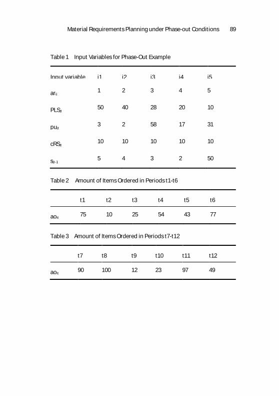
Material Requirements Planning under Phase-out Conditions 89
Table 1 Input Variables for Phase-Out Example
Input variable j1 j2 j3 j4 j5
arij 1 2 3 4 5
PLSjt 50 40 28 20 10
pujt 3 2 58 17 31
cRSjt 10 10 10 10 10
sjt-1 5 4 3 2 50
Table 2 Amount of Items Ordered in Periods t1-t6
t1 t2 t3 t4 t5 t6
aoit 75 10 25 54 43 77
Table 3 Amount of Items Ordered in Periods t7-t12
t7 t8 t9 t10 t11 t12
aoit 90 100 12 23 97 49
90 Regina Wagner and Thorsten Blecker
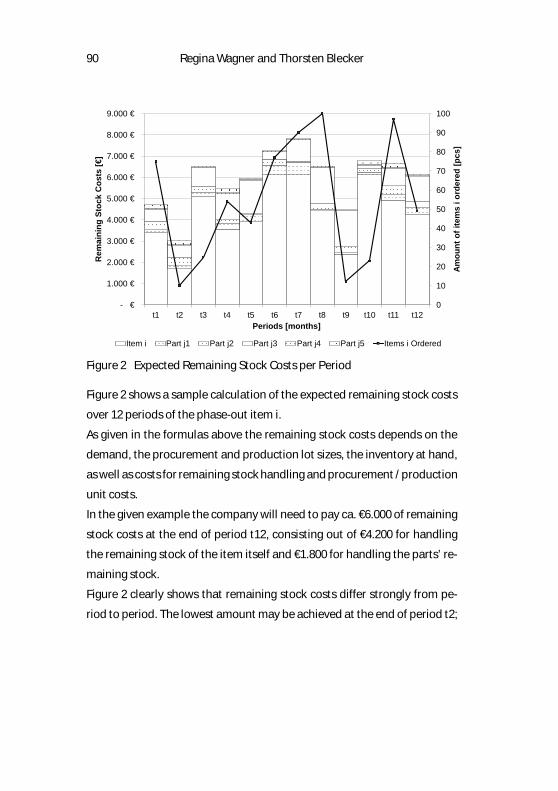
Figure 2 Expected Remaining Stock Costs per Period
Figure 2 shows a sample calculation of the expected remaining stock costs
over 12 periods of the phase-out item i.
As given in the formulas above the remaining stock costs depends on the
demand, the procurement and production lot sizes, the inventory at hand,
as well as costs for remaining stock handling and procurement / production
unit costs.
In the given example the company will need to pay ca. €6.000 of remaining
stock costs at the end of period t12, consisting out of €4.200 for handling
the remaining stock of the item itself and €1.800 for handling the parts’ re-
maining stock.
Figure 2 clearly shows that remaining stock costs differ strongly from pe-
riod to period. The lowest amount may be achieved at the end of period t2;
0
10
20
30
40
50
60
70
80
90
100
- €
1.000 €
2.000 €
3.000 €
4.000 €
5.000 €
6.000 €
7.000 €
8.000 €
9.000 €
t1 t2 t3 t4 t5 t6 t7 t8 t9 t10 t11 t12
Amou
nt o
f ite
ms
i ord
ered
[pcs
]
Rem
aini
ng S
tock
Cos
ts [€
]
Periods [months]
Item i Part j1 Part j2 Part j3 Part j4 Part j5 Items i Ordered
Material Requirements Planning under Phase-out Conditions 91
the highest amount needs to be paid at the end of period t7. The latter costs
are more than twice times period t2 costs.
5 Summary and Conclusions
This research introduces a methodology to calculate expected remaining
stock costs at end of production as add-on to material requirements plan-
ning within PPC. After a brief literature review, eleven equations are pre-
sented which serve to calculate first, the expected remaining stock quan-
tity, and second, resulting costs. An example shows the methodology’s
functionalities.
This paper closes the gap in research by addressing the missing link of
quantity and cost calculation in remaining stock investigations. By now,
only costs were analyzed, expecting remaining stock quantity as given in-
put.
Using the presented equations supports companies first of all in knowing
the expected remaining stock costs level. In a further step companies may
now decide basing on the new information to take different means for re-
ducing the expected stock. One option is to end production earlier, i.e. to
not meet the entire demand. In the example, period t2 is the month with
least remaining stock costs. Yet, the company most probably will need to
offer a penalty payment or a replacement product to the customer. This
makes choosing period t2 less likely, but period t9 could then become in-
teresting. But a further aspect changing the situation is that at the end no
remaining stock of the item itself will be available (it is not reasonable to
scrap remaining stock and pay penalty for unmet demand at the same
92 Regina Wagner and Thorsten Blecker
time), so only the parts’ remaining stock will be regarded, which would shift
it to period t10 in the given example. Yet, also the amount to be paid for not
meeting the demand needs to be considered, which consists of penalty
costs and lost profit.
Alternatively, companies might try to reduce item’s stock by selling them
to a lower (cost-covering) price and to reduce part’s stock by reducing pro-
curement lot sizes where possible. Calculating appropriate lot size
amounts is presented in Hertrampf’s (2012) publication.
The next steps in research are therefore to include unmet demand (lost
sales) and additional production runs to consume remaining parts into the
methodology. Then, companies are enabled to thoroughly decide which re-
maining stock reduction measure is the most appropriate for their given
situation.
Material Requirements Planning under Phase-out Conditions 93
References
Aurich, J.C. and Naab, C., 2006. Organization of the run-out phase in production projects. Production Engineering, XIII(1), pp.153–156.
Aurich, J.C., Naab, C. and Barbian, P., 2005. Systematisierung des Serienauslaufs in der Produktion. Zeitschrift für wirtschaftlichen Fabrikbetrieb, 100(5), pp.257–260.
Avlonitis, G.J., 1983. The product-elimination decision and strategies. Industrial Marketing Management, 12(1), pp.31–43.
Avlonitis, G.J., 1990. ‘Project Dropstrat’: product elimination and the product life cycle concept. European Journal of Marketing, 24(9), pp.55–67.
Avlonitis, G.J., Hart, S.J. and Tzokas, N.X., 2000. An analysis of product deletion sce-narios. Journal of Product Innovation Management, 17(1), pp.41–56.
Baker, M.J. and Hart, S., 2007. Product elimination. In: Product strategy and man-agement, 2nd ed. Harlow u.a.: FT Prentice Hall, pp.440–525.
Bakker, C., Wang, F., Huisman, J. and den Hollander, M., 2014. Products that go round: exploring product life extension through design. Journal of Cleaner Pro-duction, 69, pp.10–16.
Bulkeley, W.M.B.S.R. of T.W.S., 1999. IBM discloses PC pretax loss of nearly $1 billion last year. The Wall Street journal. 25 Mar.
Eckles, R.W., 1971. Product line deletion and simplification: tough but necessary de-cisions. Business Horizons, 14(5), pp.71–74.
Elbert, N., 2011. Auslaufmanagement in der Logistik - Untersuchung der Pfadab-hängigkeit im Produktlebenszyklus am Beispiel der Automobilindustrie. Veszprém, Ungarn.
Graves, S.C., 2001. Manufacturing planning and control. In: P.M. Pardalos and M.G.C. Resende, eds., Handbook of applied optimization. New York, N.Y: Oxford University Press, pp.728–746.
94 Regina Wagner and Thorsten Blecker
Grussenmeyer, R. and Blecker, T., 2014. Aligning Product Phase-Out with New Prod-uct Development. In: Grubbström, R.W.;Hinterhuber, H.H., (Eds): PrePrints, Vol-ume 1. 18th International Working Seminar on Production Economics. Inns-bruck, Austria, pp.183–194.
Grussenmeyer, R., Gencay, S. and Blecker, T., 2014. Production Phase-out During Plant Shutdown. Procedia CIRP, 19, pp.111–116.
Hackstein, R., 1989. Produktionsplanung und -Steuerung (PPS): Ein Handbuch für die Betriebspraxis. Düsseldorf: VDI.
Hertrampf, F., 2012. Auslaufmanagement in Produktionsnetzen. Berichte aus dem IPH. Garbsen, Germany: PZH.
Hertrampf, F., Nickel, R. and Nyhuis, P., 2010. Efficient phase-out planning by align-ment of lot sizes in supply chains. In: Proceedings. 43rd CIRP International Con-ference on Manufacturing Systems. Wien, pp.860–867.
Holtsch, P., 2009. Planung und Steuerung von Produktionsausläufen in der Elektro-nikindustrie. Berichte aus dem IPH. Garbsen: PZH, Produktionstechn. Zentrum.
Holzhäuer, R. and Riepl, K., 1996. Der ‘geordnete’ Produktauslauf. IO Management, 65(4), pp.49–50.
Hornung, V., 1996. Aachener PPS-Modell: Das Aufgabenmodell. 4th ed. Sonderdruck 6/94. Aachen: Forschungsinstitut für Rationalisierung (FIR).
Inness, J.G., 1994. Achieving successful product change: a handbook. Financial times. London, UK: Pitman.
Kirsch, T. and Buchholz, W., 2008. An- und Auslaufmanagement - logistische Her-ausforderungen am Anfang und Ende des Produktlebenszyklus. Industrie Man-agement, 24(3), pp.45–48.
Kotler, P. and Armstrong, G.M., 2010. Principles of marketing. 13th ed. Upper Saddle River, N.J: Pearson Education.
Lödding, H., 2005. Verfahren der Fertigungssteuerung: Grundlagen, Beschreibung, Konfiguration. Berlin: Springer.
Mitchell, M., Taylor, R. and Tanyel, F., 1998. Product elimination decisions: a com-parison of American and British manufacturing firms. International Journal of Commerce and Management, 8(1), pp.8–27.
Material Requirements Planning under Phase-out Conditions 95
Ostertag, R., 2008. Supply-Chain-Koordination im Auslauf in der Automobilindus-trie. Wiesbaden: Gabler.
Prigge, J.-K., 2008. Gestaltung und Auswirkungen von Produkteliminationen im Bu-siness-to-Business-Umfeld: eine empirische Betrachtung aus Anbieter- und Kundensicht. Wiesbaden: Gabler.
Sahyouni, K., Savaskan, R.C. and Daskin, M.S., 2010. The effect of lifetime buys on warranty repair operations. Journal of the Operational Research Society, 61(5), pp.790–803.
Saunders, J. and Jobber, D., 1988. An exploratory study of the management of product replacement. Journal of Marketing Management, 3(3), pp.344–351.
Scholz-Reiter, B., Baumbach, B. and Krohne, F., 2008. Integriertes Auslaufmanage-ment - Anforderungen an ein zielorientiertes Kennzahlensystem zur effizienten Durchführung von Produktausläufen. Industrie Management, 24(5), pp.74–78.
Schuh, G. ed., 2006. Produktionsplanung und -Steuerung: Grundlagen, Gestaltung und Konzepte. Berlin: Springer.
Slamanig, M., 2011. Produktwechsel als Problem im Konzept der Mass Customiza-tion: theoretische Überlegungen und empirische Befunde. Wiesbaden: Gabler.
Vyas, N.M., 1993. Industrial Product Elimination Decisions: Some Complex Issues. European Journal of Marketing, 27(4), pp.58–76.


![PrevalenceofMetabolicSyndromeaccordingto ...downloads.hindawi.com/journals/ecam/2012/646794.pdf · described in detail [14]. However, 2 of the previous 1,619 participants were excluded](https://img.dokumen.tips/doc/110x75/605dc21633ad5573140b4dae/prevalenceofmetabolicsyndromeaccordingto-described-in-detail-14-however.jpg)
![Biochimica et Biophysica Acta - core.ac.uk SC 29424, USA. ... as described [19]. ... gral membrane proteins in the pellet from the previous step, the samples](https://img.dokumen.tips/doc/110x75/5af912d17f8b9abd588c5d88/biochimica-et-biophysica-acta-coreacuk-sc-29424-usa-as-described-19.jpg)


