Embed Size (px)
Citation preview
University of West Bohemia in Pilsen Department of Computer Science and Engineering Univerzitni 8 30614 Pilsen Czech Republic
Holography Principles Technical report
Martin Janda, Ivo Hanák, and Václav Skala Technical Report No. DCSE/TR-2006-08 December, 2006 Distribution: public

Technical Report No. DCSE/TR-2006-08 December 2006
Holography Principles Martin Janda, Ivo Hanák, and Václav Skala
Abstract This report summarise mathematical background of the holography phenomenon along with the overview of techniques and application of the optical holography. Moreover, specialties of digital holography are presented. This report should serve as a introductory document for whomever wish to understand to holography.
This work has been partialy supported by the Ministry of Education, Youth and Sports of the Czech Republic under the research program LC-06008 (Center for Computer Graphics). This work has been partialy supported by the EU project EU within FP6 under Grant 511568 with the acronym 3DTV. Copies of this report are available on http://www.kiv.zcu.cz/publications/ or by surface mail on request sent to the following address:
University of West Bohemia in Pilsen Department of Computer Science and Engineering Univerzitni 8 30614 Pilsen Czech Republic
Copyright © 2006 University of West Bohemia in Pilsen, Czech Republic
Contents
1 Introduction 1
2 Holography physics 22.1 Wave optics . . . . . . . . . . . . . . . . . . . . . . . . . . . . . . . . . . . . 22.2 Interference . . . . . . . . . . . . . . . . . . . . . . . . . . . . . . . . . . . . 42.3 Coherence . . . . . . . . . . . . . . . . . . . . . . . . . . . . . . . . . . . . . 62.4 Elementary Waves . . . . . . . . . . . . . . . . . . . . . . . . . . . . . . . . 82.5 Diffraction . . . . . . . . . . . . . . . . . . . . . . . . . . . . . . . . . . . . . 92.6 Wave Propagation . . . . . . . . . . . . . . . . . . . . . . . . . . . . . . . . 13
2.6.1 Huygens-Fresnel Principle . . . . . . . . . . . . . . . . . . . . . . . . 132.6.2 Fresnel and Fraunhofer Approximation . . . . . . . . . . . . . . . . . 142.6.3 Diffraction Condition and Diffraction Orders . . . . . . . . . . . . . 172.6.4 Propagation in Angular Spectrum . . . . . . . . . . . . . . . . . . . 182.6.5 Propagation in Lenses . . . . . . . . . . . . . . . . . . . . . . . . . . 20
3 Optical Holography 243.1 Holography principle . . . . . . . . . . . . . . . . . . . . . . . . . . . . . . . 243.2 Inline hologram . . . . . . . . . . . . . . . . . . . . . . . . . . . . . . . . . . 263.3 Off-axis hologram . . . . . . . . . . . . . . . . . . . . . . . . . . . . . . . . . 273.4 Additional hologram types . . . . . . . . . . . . . . . . . . . . . . . . . . . . 29
3.4.1 Fourier hologram . . . . . . . . . . . . . . . . . . . . . . . . . . . . . 303.4.2 Image holograms . . . . . . . . . . . . . . . . . . . . . . . . . . . . . 313.4.3 Fraunhofer hologram . . . . . . . . . . . . . . . . . . . . . . . . . . . 31
3.5 Final notes . . . . . . . . . . . . . . . . . . . . . . . . . . . . . . . . . . . . 31
4 Digital Holography 324.1 Digital capturing . . . . . . . . . . . . . . . . . . . . . . . . . . . . . . . . . 324.2 Digital reproduction . . . . . . . . . . . . . . . . . . . . . . . . . . . . . . . 324.3 Hologram Synthesis . . . . . . . . . . . . . . . . . . . . . . . . . . . . . . . 334.4 Hologram Reconstruction . . . . . . . . . . . . . . . . . . . . . . . . . . . . 34
4.4.1 Diffraction pattern reconstruction . . . . . . . . . . . . . . . . . . . 344.4.2 Retrieval of Phase and/or Amplitude . . . . . . . . . . . . . . . . . . 34
i

Chapter 1
Introduction
Holography is quite old scientific field. As an inventor of holography could be claimedprof. D. Gabor [Gab49]. He proposed holographic imaging when working on enhancingresolution of electron microscopy. However, the first holograms produced poor qualityimages and the development of holography stagnated for a while. The technology wasgreatly improved after introduction of the off-axis holograms and invention of the LASERin sixties. Since then, holography found many applications including 3D imaging andinterferometry. Optical holography is introduced in the Section 3.
The efforts for bringing holography to the digital world of computers are not neweither. The first attempts were already done in 1967, however, the first useful results hadto wait for sufficient computational power which has been achieved not until nineties ofthe 20th century. For example, the first digital holograms computed at interactive rateswere described in 1994 in [Luc94]. Digital holography is introduced in the Section 4.
Holography is built on quite complex physical laws of optics. These laws are referencedmany times in the text of this thesis and therefore basics of the wave optics are providedin the Section 2 of this chapter. The described topics are wave equation, interference,coherence and diffraction.
1
Chapter 2
Holography physics
The whole holography relies heavily on quite complex rules and laws of wave optics. Waveoptics considers light as an electromagnetic wave of an arbitrary wavelength in general.However, the most interesting, in the context of this thesis, is the interval ranging from300 to 700 nm because this interval constitutes the visible light. Visible light, just lightfrom now on, interacts with its surroundings and with itself at microscopic levels and ina quite complex manner. This interaction is referred as interference. The interference inparticular is described in the section 2.2.
The principle of the interference phenomenon is based on the wave nature of thelight and therefore a short introduction into the mathematics of waves is provided in thesection 2.1. The relation of the wave calculus to the physics of light is also presented there.
From interference the more complex phenomenon of diffraction is derived. The diffrac-tion is responsible for forming the object beam on a photographic plate, see the Section 3for reference. The exact mathematical model of the diffraction was not found yet. However,there are some approximated models but, though approximated, they provide sufficientlyaccurate results. The diffraction models are introduced in the Section 2.5.
2.1 Wave optics
The light is, in general, an electromagnetic wave of some wavelength spectrum. The visiblelight is on the interval ranging from 300 nm to 700 nm. The light with wavelength longerthan 700 nm is called infrared and light with wavelength shorter than 300 nm is calledultraviolet. The visible band is, of course, the most interesting one since it is visible by ahuman observer.
The electromagnetic wave consists of the time varying electric and magnetic fieldswhich are tightly coupled as it is evident from Maxwell’s equations. These simplifiedMaxwell’s equations Equation (2.1), Equation (2.2) applies for vacuum:
∇ ·E = 0 (2.1)∇ ·H = 0 (2.2)
∇×E = −µ0∂H∂t
(2.3)
∇×H = ε0∂E∂t
(2.4)
2
CHAPTER 2. HOLOGRAPHY PHYSICS 3
The notation in the Maxwell’s equations is following: the E denotes electric field, Hdenotes magnetic field, µ0 denotes permeability of vacuum, ε0 denotes permittivity ofvacuum, ∇· denotes divergence operator and ∇× denotes curl operator. The solution ofthose Maxwell equations are two sinusoidal plane waves, with the electric and magneticfield directions orthogonal to one other and the direction of travel, and with two fields inphase, travelling at the speed of light in vacuum.
By rewriting the Maxwell’s simplified equations, one obtains the equations:
∇2E = µ0ε0∂2
∂t2E (2.5)
∇2B = µ0ε0∂2
∂t2B (2.6)
The equations Equation (2.5) and Equation (2.6) are vector equations, but under somecircumstances, all components of the vectors behaves exactly the same and a single scalarequation can be used to describe the behavior of the electromagnetic disturbance. Thescalar equation can be written in this form:
∇2u(p, t)− n2
c2
∂2u(p, t)∂t2
= 0, (2.7)
where u(p, t) represents a scalar field component at the given position p and time t ex-amined in a material of refractive index n. The light travels through this material at aspeed of c/n, where c is a speed of light.
The Equation (2.7) describes the behavior of a wave in a linear, uniform, isotropic,homogeneous, and non-dispersive material and it is a base for the scalar wave theory thatserves as base upon which all assumptions in this thesis are build on. Even thought thescalar wave theory is an approximation rather than an exact description it is satisfactorilyas it describes the behavior of the light wave in concordance with physical experiments.The error introduced by the approximation is small and it is recognisable only at thedistance of few wavelengths from the aperture’s boundary.
A time-varying scalar field for a monochromatic wave in the scalar wave theory atposition P is:
u(p, t) = A(p) cos[2πνt− ϕ(p)], (2.8)
where ν is an optical frequency of the wave in [Hz], A(p) and ϕ(p) defines amplitudeand phase respectively of the wave at the position p. This equation describes the waveproperly yet the more convenient notation is:
u(p, t) = <{u(p) exp(−i2πνt)} = <{u(p) exp(−iωt)} ,
u(p, t) = u(p) exp(−i2πνt), (2.9)
where ω is an angular speed and u(p) is a complex amplitude defined as:
u(p) = A(p) exp[iϕ(p)]. (2.10)
The function u(p, t) is known as the wavefunction. A term diffraction pattern refersto an array a complex notations for a wavefunction u(p, t) defined by the Equation (2.9).The wavelength of a light is defined as λ = c/nν = λ0/n, where λ0 is a wavelength in avacuum. The following text assumes the propagation is done in a vacuum, if not notedotherwise.

CHAPTER 2. HOLOGRAPHY PHYSICS 4
A wave defined by the Equation (2.9) has to satisfy the scalar wave theory, i.e. Equa-tion (2.7). If the Equation (2.9) is substituted into the scalar wave theory a relation knownas the Helmholtz equation is obtained:
(∇2 + k2)u(p) = 0, (2.11)
where k = 2π/λ is known as a wavenumber. A solution to the Helmholtz equationdefines waves of various forms including basic ones such as planar wave and sphericalwave that are described further in the text. Note, that the Helmholtz equation describesonly a spatial part of a complete solution thanks to the fact that u(p, t) is separable, i.e.u(p, t) = u(p)t(t). The temporal part of the solution is a linear combination of sine andcosine function and thus it is not considered in following sections.
The relation between the ray and the wave optics is straightforward. A relation isclearly visible from the specification of a wavefront. Wavefront is an iso-surface thatconsist of points with wave function samples of the same phase, i.e. ϕ(p) = 2πq, q ∈ 〈0; 1〉.A gradient of the phase ϕ is a normal of the wavefront’s surface at a given point p. Besidesthat it gives a direction of a local propagation for the wave and thus it gives a directionof a ray in a ray optics [Kra04].
Another important feature of the light is its optical power. This is important whencreating of a final image because it defines an amount of energy delivered to a photographicmaterial and/or sensor. Optical intensity is defined as a time average of an amount ofenergy that crosses an unit perpendicular to the energy flow during a unit of time. If thetime period is short enough the intensity of wave u(p) is equal to |u|2, i.e. it is a complexmultiplication of u with its complex conjugate [Har96]:
I = u(p)u∗(p) = |u(p)|2. (2.12)
For computing a hologram, one has to compute the light field at the hologram planefirst and then the optical intensity is evaluated to create the actual interference patternor fringe pattern.
2.2 Interference
In the Section 2.1 the light was described as a wave. However, there is rarely just onewave present in a space. There are usually many waves and each one can interact withthe other. This interaction is called interference.
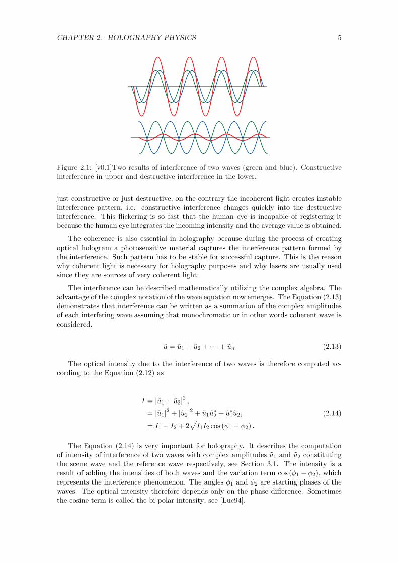
The simplest situation is if two waves travel in the same direction. According to thephase of each wave the resulting electrical intensity will increase or decrease. If phases atsome point in a space are the same or near the same, the constructive interference occursat that point. If the phases are opposite or almost opposite the destructive interferenceoccurs, see FigureFigure 2.1.
As a result the optical intensity due to two interfering waves is increased in the caseof constructive interference and decreased in the case of destructive interference. This isquite surprising result that by adding two lights one can obtain less or none light. Howeverthis is true for the coherent light only.
The coherence is described in the Section 2.3 but it basically determines the stability ofthe interference effect in time. The coherent light produces stable interference pattern, i.e.
CHAPTER 2. HOLOGRAPHY PHYSICS 5
Figure 2.1: [v0.1]Two results of interference of two waves (green and blue). Constructiveinterference in upper and destructive interference in the lower.
just constructive or just destructive, on the contrary the incoherent light creates instableinterference pattern, i.e. constructive interference changes quickly into the destructiveinterference. This flickering is so fast that the human eye is incapable of registering itbecause the human eye integrates the incoming intensity and the average value is obtained.
The coherence is also essential in holography because during the process of creatingoptical hologram a photosensitive material captures the interference pattern formed bythe interference. Such pattern has to be stable for successful capture. This is the reasonwhy coherent light is necessary for holography purposes and why lasers are usually usedsince they are sources of very coherent light.
The interference can be described mathematically utilizing the complex algebra. Theadvantage of the complex notation of the wave equation now emerges. The Equation (2.13)demonstrates that interference can be written as a summation of the complex amplitudesof each interfering wave assuming that monochromatic or in other words coherent wave isconsidered.
u = u1 + u2 + · · ·+ un (2.13)
The optical intensity due to the interference of two waves is therefore computed ac-cording to the Equation (2.12) as
I = |u1 + u2|2 ,
= |u1|2 + |u2|2 + u1u∗2 + u∗1u2,
= I1 + I2 + 2√
I1I2 cos (φ1 − φ2) .
(2.14)
The Equation (2.14) is very important for holography. It describes the computationof intensity of interference of two waves with complex amplitudes u1 and u2 constitutingthe scene wave and the reference wave respectively, see Section 3.1. The intensity is aresult of adding the intensities of both waves and the variation term cos (φ1 − φ2), whichrepresents the interference phenomenon. The angles φ1 and φ2 are starting phases of thewaves. The optical intensity therefore depends only on the phase difference. Sometimesthe cosine term is called the bi-polar intensity, see [Luc94].
CHAPTER 2. HOLOGRAPHY PHYSICS 6
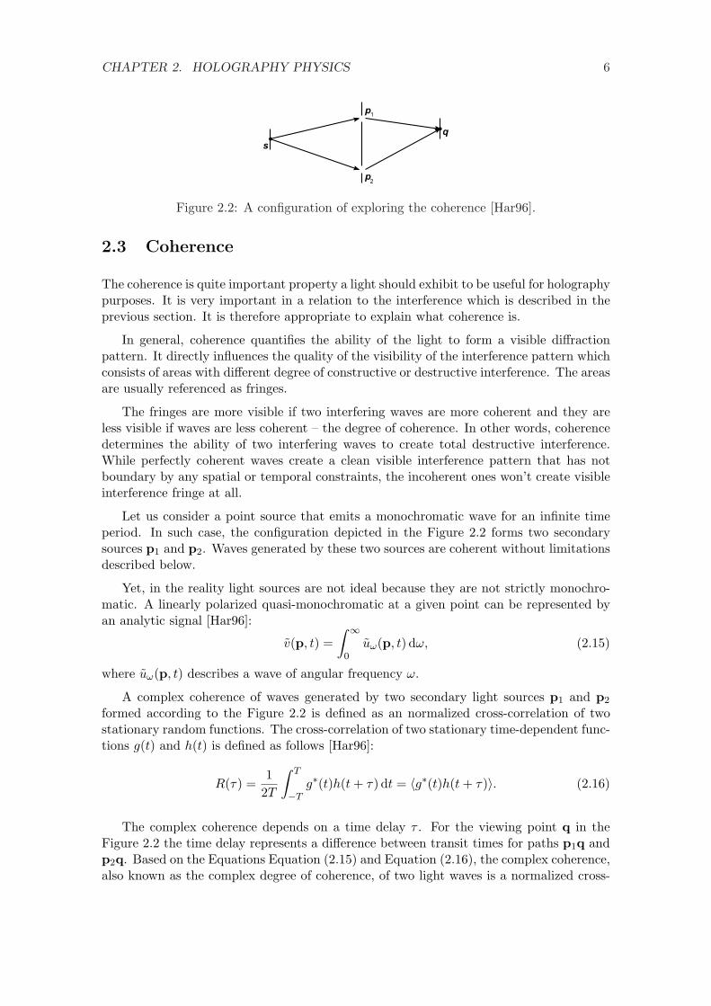
Figure 2.2: A configuration of exploring the coherence [Har96].
2.3 Coherence
The coherence is quite important property a light should exhibit to be useful for holographypurposes. It is very important in a relation to the interference which is described in theprevious section. It is therefore appropriate to explain what coherence is.
In general, coherence quantifies the ability of the light to form a visible diffractionpattern. It directly influences the quality of the visibility of the interference pattern whichconsists of areas with different degree of constructive or destructive interference. The areasare usually referenced as fringes.
The fringes are more visible if two interfering waves are more coherent and they areless visible if waves are less coherent – the degree of coherence. In other words, coherencedetermines the ability of two interfering waves to create total destructive interference.While perfectly coherent waves create a clean visible interference pattern that has notboundary by any spatial or temporal constraints, the incoherent ones won’t create visibleinterference fringe at all.
Let us consider a point source that emits a monochromatic wave for an infinite timeperiod. In such case, the configuration depicted in the Figure 2.2 forms two secondarysources p1 and p2. Waves generated by these two sources are coherent without limitationsdescribed below.
Yet, in the reality light sources are not ideal because they are not strictly monochro-matic. A linearly polarized quasi-monochromatic at a given point can be represented byan analytic signal [Har96]:
v(p, t) =∫ ∞
0uω(p, t) dω, (2.15)
where uω(p, t) describes a wave of angular frequency ω.
A complex coherence of waves generated by two secondary light sources p1 and p2
formed according to the Figure 2.2 is defined as an normalized cross-correlation of twostationary random functions. The cross-correlation of two stationary time-dependent func-tions g(t) and h(t) is defined as follows [Har96]:
R(τ) =1
2T
∫ T
−Tg∗(t)h(t + τ) dt = 〈g∗(t)h(t + τ)〉. (2.16)
The complex coherence depends on a time delay τ . For the viewing point q in theFigure 2.2 the time delay represents a difference between transit times for paths p1q andp2q. Based on the Equations Equation (2.15) and Equation (2.16), the complex coherence,also known as the complex degree of coherence, of two light waves is a normalized cross-
CHAPTER 2. HOLOGRAPHY PHYSICS 7
correlation between v1 and v2 [Har96]:
γ12(τ) =〈v1(t + τ)v∗2(t)〉
[〈v1(t)v∗1(t)〉〈v2(t)v∗2(t)〉]1/2=〈v1(t + τ)v∗2(t)〉
(I1I2)1/2(2.17)
The amplitude |γ12(τ)| of complex coherence that describes a light in terms of coherency.If |γ12(τ)| = 1 then the light is considered as a coherent one, if |γ12(τ)| = 0 then the lightis incoherent. For other values between these two extremes, the light is said to be partiallycoherent.
According to the configuration of secondary point sources p1 and p2 and their distancethe source s it is possible to distinguish between two cases of coherence: a spatial and atemporal coherence. Both meanings for the coherence explores conditions for which theinterference pattern, i.e. fringes, becomes invisible and thus useless for the purposes ofthe holography.
If two ideal and coherent light sources of intensities I1 and I2 forms an interferencepatterns of intensity I then the visibility V of such pattern is [Har96]:
V =2(I1I2)1/2
I1 + I2cos(ψ), (2.18)
where ψ is an angle between electrical vectors of both light waves and thus representspolarization1.
For partially coherent light sources of same intensity, i.e. I1 = I2, the visibility of theinterference pattern is [Har96]:
V = |γ12(τ)|. (2.19)
The temporal coherence becomes important for a very small quasi-monochromaticlight sources. For such light sources, the complex coherence depends on a difference intransit times between each of secondary sources p1 and p2 and the primary source s.Thus, it is, in fact, a normalised autocorrelation of the function v(t). If requirements forthe Equation (2.19) are fulfilled, the amount of coherence can be determined from thevisibility V of fringes. According to [Har96], for a radiation with a mean frequency ν0
and bandwidth ∆ν the visibility V drops to zero if difference in transit times ∆τ fulfillfollowing condition:
∆τ∆ν ≈ 1, (2.20)
where ω = 2πν. The time ∆τ is denoted as a coherence time of given radiation. Anotherforms of this property is a coherence length. If the optical path difference is smaller thanthe coherence length the interference pattern is visible. The coherence length ∆l for aradiation of mean wavelength λ0 and wavelength bandwidth ∆λ is:
∆l ≈ c∆τ ≈ c/∆ν ≈ λ20/∆λ. (2.21)
Spatial coherence becomes an important feature of the radiation as the difference ofoptical paths sp1 and sp2 is small enough for the time difference to be τ ≈ 0. Spatialcoherence relates a range between two points and visibility of the interference pattern. Iftwo slits p1 and p2 are separated by a distance greater than the diameter of the coherencearea then waves generated by these two slit do not form visible interference pattern.
1Note, that the visibility drops to zero if ψ = π/2, i.e. waves of polarized light do not create a visibleinterference pattern if polarization directions are perpendicular to each other.

CHAPTER 2. HOLOGRAPHY PHYSICS 8
It can be shown that for a extended distant source, i.e. source composed of many pointsources, the visibility V is proportional to an absolute value of the sinc function [Wei]. Theargument of the sinc function is proportional to a multiply of distance a between slits andan angle η that is a range in which the individual point sources subtends the screen. Ifeither a or η increases then the fringe visibility decreases. Note, that for an angle η = 0that is valid for a point source the sinc function does not depend on distance a.
The spatial complex coherence can be expressed in terms of Fourier transform as well.If the distance between two points p1 = (0, 0, z) and p2 = (x, y, z) is much smaller thanthe distance from these points to a source s then the complex coherence of the fieldfollows [Har96]:
µ12 =exp(iφ12)
∫∫S I(ξ, η) exp[ik(xξ + yη)] dξ dη∫∫
S I(ξ, η) dξ dη, (2.22)
where ξ = xS/z, η = yS/z, plane S is a XY-plane that contains the source and φ12 =−k(x2 + y2)/2z.
An important side effect of the coherence is that if the light is coherent in both spatiallyand temporally, it is possible to omit the temporal component −iωt of the wavefunctiondefined by the Equation (2.9) and leave only the wave distribution to be examined orcomputed. This can be interpreted as exploration of the wave distribution for an infinitelysmall time period. As the intensity I that serves as the physically measurable propertyof the light depends only on the complex amplitude u(p) for the monochromatic light, nounacceptable approximation is applied by that. Thus, in the following text the complexamplitude serves as a full description of the monochromatic wave distribution, if not notedotherwise.
2.4 Elementary Waves
Elementary waves represents the simplest solution for the Helmholtz equation. Thereare two forms of these waves: a planar wave and a spherical wave. The plane wave isa wave with wavefronts that are infinite planes. The complex amplitude of such waveis [Gra03, Kra04]:
u(r) = a exp(ik · r)= a exp[i(kxx + kyy + kzz)], (2.23)
where k = (kx, ky, kz) is a wavevector and a is a complex envelope that defines the phaseand the amplitude at the origin of the wave. The vector r = (x, y, z) points from theorigin to a sample for which a distribution is obtained. The length of the wavevector isequal to the wavenumber. Intensity of the wave is constant and it is equal to I = |a|2.Wavefunction of the planar wave is then following:
u(r, t) = |a| cos(arg{a}+ k · r− ωt). (2.24)
The spherical wave is a wave where wavefronts have a form of concentric sphericalsurfaces centered at the point source. The complex amplitude of the spherical wave withan origin identical to the source of the field is:
u(r) =a
rexp(ikr), (2.25)

CHAPTER 2. HOLOGRAPHY PHYSICS 9
Figure 2.3: Relation between spherical and planar wave [Kra04].
where r = |r|, i.e. it is a distance from the source. The fraction a/r compensates thatfact that the surface of the spherical surface grows quadratically. If the intensity, i.e. |a|2,was not modified at all then it means that the intensity per unit grows quadratically aswell. Yet, a wave cannot increase its energy on its own. Thus, the complex amplitude ahas to be modified by 1/r to compensate the quadratical growth of the surface2 in theEquation (2.25).
The relation between the planar and the spherical wave is more apparent when thewave propagates further from the point source. If an observation is done along the Z-axisthrough a window which is constant in size spherical wavefronts becomes a planar as it isdepicted in the Figure 2.3. This means that if the distance is large enough in comparisonto extents in X-axis and Y-axis it is possible to approximate the spherical wave with theparaboloidal wave. This is a mechanism utilized by the Fresnel approximation, see below.If the distance increases even further it is possible to approximate the spherical wave withthe planar one.
2.5 Diffraction
The Diffraction is basically the same phenomenon as the interference. The differenceis that the interference is referenced in a case of superposition of several light sourcesand diffraction is referenced in a case of superposition of many sources. In the case ofholography, the interference is usually addressed when interference of the scene light fieldand the reference beam is evaluated and the diffraction is addressed when light field of ascene is evaluated.
The nature of the diffraction can be illustrated on the well known Huygens principleproposed by C. Huygens. This principle states that the wavefront of a disturbance in atime t+∆t is an envelope of wavefronts of a secondary sources emanating from each pointof the wavefront in a time t, see Figure 2.4 for reference. This principle was modified by A.Fresnel who stated that the secondary sources interfere with each other and the amplitudeat each point of the wavefront is obtained as superposition of the amplitudes of all thesecondary wavelets. This Huygens-Fresnel principle matches many optical phenomenaand it was also shown by G. Kirchhoff how this principle can be deduced from Maxwell’sequations.
Although this principle works in many cases its validity is in question. For example,it does not determine the direction of the wavefront propagation. It is only an intuitivechoice that the wavefront diverges from the source and not converges back to the sourcedepending on the chosen orientation of the envelope of the secondary wavelets. In this
2Note, that the intensity grows quadratically with the magnitude of the complex amplitude

CHAPTER 2. HOLOGRAPHY PHYSICS 10
Figure 2.4: [v0.5]Huygens principle demonstrated on spherical (left) and planar (right)waves.
work, as in many others, this principle is accepted as an appropriate description of the wavebehavior of the light and its inadequacies are neglected. Some of the synthesis methodsare based on this principle.
The intuitive way of the diffraction understanding is covered by the Huygens principlebut more formal descriptions also exists. Some of them are presented in the followingmaterial.
The mathematical description of the diffraction is quite difficult. It’s due to the vecto-rial nature of the problem and many propagation medium properties like linearity, isotropy,homogeneity or dispersiveness that increase dimension of the problem. The basic diffrac-tion model assumes an ideal material that is linear, isotropic, homogeneous, nondispersiveand nonmagnetic. Under these conditions, the electromagnetic wave behavior can bedescribed using only one scalar equation that described behavior of both magnetic andelectric field. There is one other condition that further simplifies the diffraction model:diffraction structures that are large compared to the wavelength of the diffracted wave.All those simplifications and constraints turn the diffraction model into approximationbut even thought simplifications are significant they causes only small loss of accuracyand thus they are more then appropriate in many situations.
There are two fundamental description of the diffraction: the Kirchhoff formulationand the Rayleigh-Sommerfeld formulation [Goo05, LBL02]. Both formulations describethe field in front of a screen or an aperture properly and accurately. Nevertheless, theKirchoff one has a certain limitation as it fails when the point closes to the screen for adistance lower than few wavelengths. Also, it assumes that the field behind the apertureis zero and this is in contradiction with physical experiments. Despite its limitations, theKirchoff formulation is widely used in practice.
The Kirchhoff formulation of diffraction is based on the integral theorem of Helmholtzand Kirchoff. It states that the field at any point can be expressed in terms of wave valueson any closed surface surrounding that point [Goo05]. The theorem is an application ofthe Green’s theorem and the Helmholtz equation. While the Helmholtz equation describebehavior of waves, the Green’s theorem defines a relation between two complex functionsu(p) and g(p) of position, closed volume V in which the observation is performed, arbitraryboundary surface S that encloses V , and derivatives of functions u and g along inwardnormal n of boundary surface S:
−∫∫
S
∂u
∂ng − u
∂g
∂nds =
∫∫∫
Vg∇2u− u∇2g dv, (2.26)
where functions u(p) and g(p) provides twice continuously differentiable scalar fields map-
CHAPTER 2. HOLOGRAPHY PHYSICS 11
pings between V and S. If both functions satisfy the Helmholtz equation then [LBL02]:
−∫∫
S
∂u
∂ng − u
∂g
∂nds = 0 (2.27)
The goal of the Kirchoff formulation is do find a field at a point p0. For such purposeit uses a boundary surface on a one side of the aperture. This boundary surface consistof two parts: a plane Sp close to the aperture including its transparent portion Σ anda spherical surface Sε. Next, a set of boundary condition known as Kirchhoff boundaryconditions3 that describes behavior of field u in close neighborhood to the screen. Theinfluence of the spherical surface vanishes as the radius of the spherical surface increasestowards infinity [BW05]. By application of there condition the Equation (2.27) is simplifiedto:
u(p0) =14π
∫∫
Σ
(∂u
∂ng − u
∂g
∂n
)ds, (2.28)
where Σ is a transparent portion of the screen, u is a complex function describing the wavedistribution and g is a complex function, see below.
A further simplification of the Equation (2.28) is based on use of a proper Green’sfunction instead of the function g in the Equation (2.27). Such function that satisfies theHelmholtz equation is:
g(p1) =exp(ikr01)
r01,
where r01 = p0 − p1 and r01 = |r01|. The derivation along normal can be approximatedaccording to an assumption on distances between observation point p0 in enclosed volumeand point p1 on the surface Σ. If r01 À λ then:
∂g
∂n=
exp(ikr01)r01
(ik − 1
r01
)cos(n, r01)
≈ ikexp(ikr01)
r01cos(n, r01).
Also, it is assumed that the screen or the aperture is illuminated by a spherical waveemerging from the point p2. Hence, the field u at the point p1 is:
u(p1) =a exp(ikr21)
r21,
where r21 is distance between p1 and p2.
Application of assumptions and substitutions described above leads to a form knownas the Fresnel-Kirchhoff diffraction formula:
u(p0) =a
iλ
∫∫
Σ
exp[ik(r21 + r01)]r21r01
[cos(n, r01)− cos(n, r21)
2
]ds, (2.29)
where a is basic amplitude/phase of the spherical wave, n is a normal of transparentportion Σ of the planar screen, and cos(a,b) is a cosine of angle between vectors a and b.
3The first assumption is that the distribution of the field u across the surface Σ including its derivatealong normal n is no different from the same configuration without the screen. The second assumption isthat a portion of the surface close to the screen Sp−Σ lies in a geometrical shadow an thus the function uas well as its derivate along the normal is zero. Both assumption are not physically valid as they are neverfulfilled completely but they simplifies the equation by replacing of enclosing surface just with the surfaceΣ. For more details, refer to [Goo05].
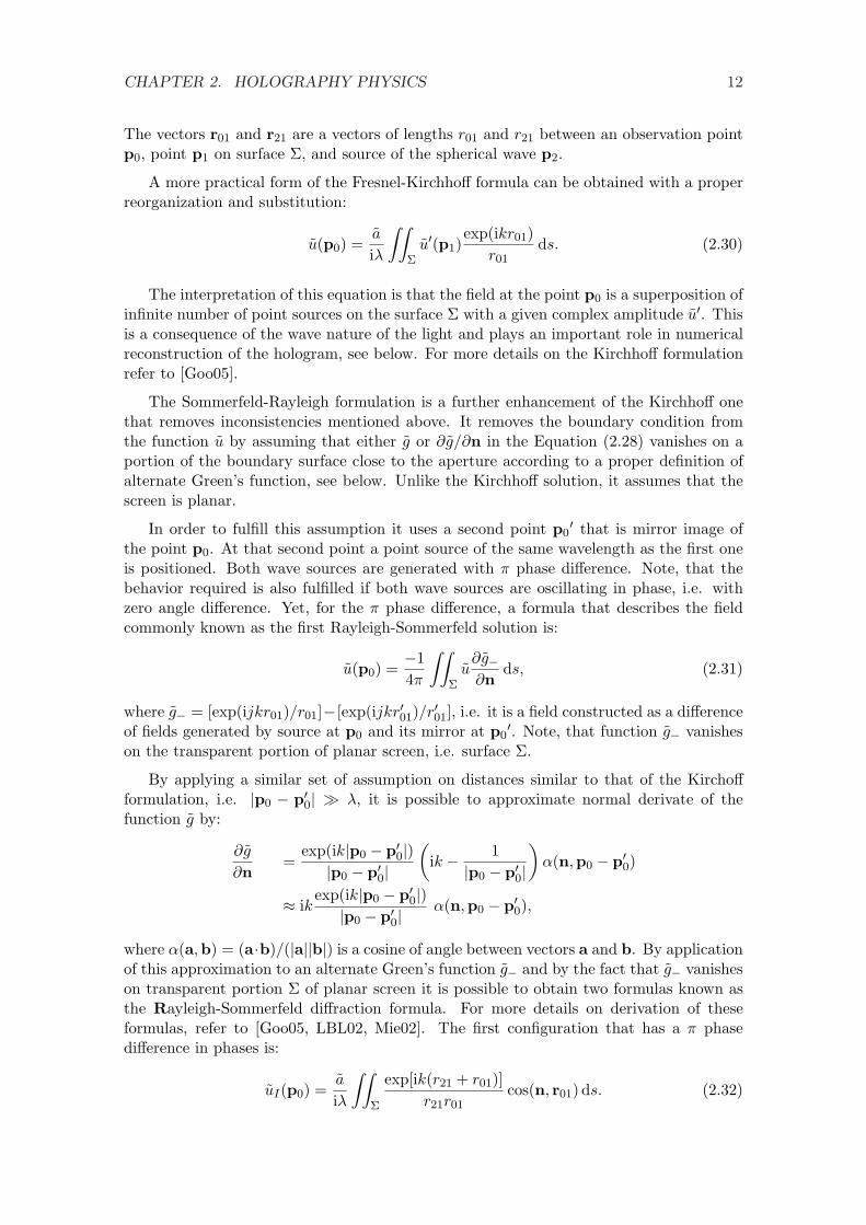
CHAPTER 2. HOLOGRAPHY PHYSICS 12
The vectors r01 and r21 are a vectors of lengths r01 and r21 between an observation pointp0, point p1 on surface Σ, and source of the spherical wave p2.
A more practical form of the Fresnel-Kirchhoff formula can be obtained with a properreorganization and substitution:
u(p0) =a
iλ
∫∫
Σu′(p1)
exp(ikr01)r01
ds. (2.30)
The interpretation of this equation is that the field at the point p0 is a superposition ofinfinite number of point sources on the surface Σ with a given complex amplitude u′. Thisis a consequence of the wave nature of the light and plays an important role in numericalreconstruction of the hologram, see below. For more details on the Kirchhoff formulationrefer to [Goo05].
The Sommerfeld-Rayleigh formulation is a further enhancement of the Kirchhoff onethat removes inconsistencies mentioned above. It removes the boundary condition fromthe function u by assuming that either g or ∂g/∂n in the Equation (2.28) vanishes on aportion of the boundary surface close to the aperture according to a proper definition ofalternate Green’s function, see below. Unlike the Kirchhoff solution, it assumes that thescreen is planar.
In order to fulfill this assumption it uses a second point p0′ that is mirror image of
the point p0. At that second point a point source of the same wavelength as the first oneis positioned. Both wave sources are generated with π phase difference. Note, that thebehavior required is also fulfilled if both wave sources are oscillating in phase, i.e. withzero angle difference. Yet, for the π phase difference, a formula that describes the fieldcommonly known as the first Rayleigh-Sommerfeld solution is:
u(p0) =−14π
∫∫
Σu
∂g−∂n
ds, (2.31)
where g− = [exp(ijkr01)/r01]−[exp(ijkr′01)/r′01], i.e. it is a field constructed as a differenceof fields generated by source at p0 and its mirror at p0
′. Note, that function g− vanisheson the transparent portion of planar screen, i.e. surface Σ.
By applying a similar set of assumption on distances similar to that of the Kirchoffformulation, i.e. |p0 − p′0| À λ, it is possible to approximate normal derivate of thefunction g by:
∂g
∂n=
exp(ik|p0 − p′0|)|p0 − p′0|
(ik − 1
|p0 − p′0|)
α(n,p0 − p′0)
≈ ikexp(ik|p0 − p′0|)
|p0 − p′0|α(n,p0 − p′0),
where α(a,b) = (a·b)/(|a||b|) is a cosine of angle between vectors a and b. By applicationof this approximation to an alternate Green’s function g− and by the fact that g− vanisheson transparent portion Σ of planar screen it is possible to obtain two formulas known asthe Rayleigh-Sommerfeld diffraction formula. For more details on derivation of theseformulas, refer to [Goo05, LBL02, Mie02]. The first configuration that has a π phasedifference in phases is:
uI(p0) =a
iλ
∫∫
Σ
exp[ik(r21 + r01)]r21r01
cos(n, r01) ds. (2.32)

CHAPTER 2. HOLOGRAPHY PHYSICS 13
The second configuration that has zero phase difference in phases is:
uII(p0) = − a
iλ
∫∫
Σ
exp[ik(r21 + r01)]r21r01
cos(n, r21) ds. (2.33)
Note, the both the first and the second RayLeigh-Sommerfeld resembles the Kirchhoff-Fresnel diffraction formula with the difference in sign and the last cosine-based component.It can be shown that the Kirchoff solution is an average of both the first and the secondRayleigh-Sommerfeld solution. Kirchoff and Rayleigh-Sommerfeld solutions are almostidentical for small angles and larger distance but they differs for distances closer to theaperture. For more detail on comparison and discussion on consequences beyond scope ofthis work, refer to [Goo05].
2.6 Wave Propagation
The propagation of the wave in a free space plays an important role in the hologram re-construction as it is required for presenting of optical field or diffraction pattern generatedby a screen and/or aperture to the viewer. The propagation is driven by the Helmholtzequation and the Huygens-Fresnel principle.
Basically, the propagation of the wave is reflected in a change in the phase. Yet, itis a question whether the changes should be introduces by adding or subtracting a valuefrom the phase. As the time dependent component exp(−iωt) of the wavefunction in theEquation (2.9) rotates in a clockwise direction waves emitted earlier in time have phasegreater than waves emitted later. The later the wave is emitted the closer it is to itssource. Thus, if waves are to be propagated from the source then the phase has to beincreased.
In order to minimize the confusion from signs of phases, it is assumed that the prop-agation of the wave is examined in direction of a positive Z-axis. This also simplifiesequation for propagation in a direction parallel to the Z-axis. If other configuration isrequired then it is always possible to transform the scene to fit the requirement.
2.6.1 Huygens-Fresnel Principle
The Huygens-Fresnel principle4 states that every point on a primary wavefront is a sourceof spherical waves with the same optical frequency and the primary wave is. The resultingfield is a superposition of these secondary waves defined by their complex amplitude and/orwavefunction [Wei].
The Huygens-Fresnel principle is confirmed by both Kirchoff and Rayleigh-Sommerfelddiffraction formulas. Using the first Rayleigh-Sommerfeld solution from the Equation (2.32),the Huygens-Fresnel principle is [LBL02]:
uI(p0) =1iλ
∫∫
Σu(p1)
exp(ikr01)r01
cos θ ds, (2.34)
4Original Huygens principle describes a new wavefront as an envelope of spherical wave sources generatedon a surface of the previous wavefront. Yet, this is not physically valid as it may ignore obstacles in wavepropagation and it allows a creating of back-waves.

CHAPTER 2. HOLOGRAPHY PHYSICS 14
where u(p1) represents a secondary point source positioned at the point p1 within theaperture Σ. The complex amplitudes of the secondary sources are proportional to theamplitude at the point p1 of the original wave and the phase leads the phase of the originalwave by π/2 due to factor 1/i. Note, that due to the Rayleigh-Sommerfeld solution, theaperture Σ is expected to be a plane or its portion and thus all following solutions forthe wave propagation solve the problem of propagating between two parallel planes, if notnoted otherwise.
The important aspect of the Equation (2.34) is that it is basically a convolution integralas it can be expressed as follows:
u(p0) =∫∫
Σh(p0,p1)u(p1) ds, (2.35)
where h(p0,p1) is the impulse response function that is given explicitly by:
h(p0,p1) =1iλ
exp(ikr01)r01
cos θ.
2.6.2 Fresnel and Fraunhofer Approximation
As noted in previous subsections, it is possible to express the Huygens-Fresnel principlein terms of the first Rayleigh-Sommerfeld solution. The angle θ is an angle between theoutward normal n and the vector r01. The cosine of this angle can be also expressed asfollowing:
cos θ =z
r01,
and if a configuration is that of the Figure 2.5 it is possible to express the Huygens-Fresnelprinciple as following:
u(x, y) =z
iλ
∫∫
Σu(ξ, η)
exp(ikr01)r201
dξ dη, (2.36)
where r01 = [z2 + (x − ξ)2 + (y − η)2]1/2. Besides that, if the distance z is greater thanthe extent in the X-axis and Y-axis then cosθ ≈ 1 and thus the whole cosine term can beomitted completely. Nevertheless, at the end both approaches lead to the same equations.All following approximations simplifies the expression for r01 because it contains squareroot function that does not allows use of the Fourier transform that greatly reduces thecomputation complexity of the expression.
The first approximation is known as the Fresnel approximation. It is based on avalue of the Z-axis component of r01 that, if large enough, allows application of binomialexpansion for the square root function. In order to apply the assumption, first, a reorderingof the expression for the distance r01 has to be applied:
r01 = z
[1 +
(x− ξ
z
)2
+(
y − η
z
)2]1/2
. (2.37)
Such expression now resembles a an expression√
1 + b, where |b| < 1. This expression canbe decomposed by use of a binomial expansion to a form:
√1 + b = 1 +
12b− 1
8b2 + . . . . (2.38)

CHAPTER 2. HOLOGRAPHY PHYSICS 15
Figure 2.5: Configuration of the Fresnel/Fraunhofer approximation [Goo05].
If the extent in Z-axis is greater than the extent in both X-axis and Y-axis, i.e. ifit is valid that z À (x − ξ)2 + (y − η)2, then it is possible to apply the approximationby dropping the third component of the binomial expansion in the Equation (2.38). Inorder to avoid the degradation of the result, the third term shall not cause a change in thedistance greater than 1◦ if applied to the phase in the Equation (2.36) because the wavepropagation is sensitive to the phase [MNF+02]. This is fulfilled if the following conditionis valid:
z3 À k
8[(x− ξ)2 + (y − η)2]2max, (2.39)
where k = 2π/λ is a wavenumber. Note, that this condition requests a viewing distanceof z À 250 mm for a circular aperture of diameter 10 mm is observed from a region of size1 cm and the wavelength is λ = 0.5 µm. If z fulfills the condition the viewer is known tobe in a near field or Fresnel region.
The above mentioned condition is sufficient but it is also very strict. In fact it is overlystrict. As it is shown in [Goo05] for a diffraction aperture illuminated with an uniformplane wave the Fresnel approximation is valid even for closed distances than distancesforced by the Equation (2.39).
Nevertheless, by fulfilling the condition it is possible to apply the Equation (2.37) tothe first two components of the binomial expansion according to the Equation (2.38) andobtain:
r01 ≈ z +(x− ξ)2 + (y − η)2
2z. (2.40)
Then, this approximation of the distance r01 is applied for the phase component in theEquation (2.36) as it is required to keep it as accurate as possible. As the distance in thephase is multiplied by a wavenumber k ≈ 107 a small error in r01 may cause significantchange in phase. The distance used in the denominator is approximated by much coarserapproximation because it modifies only the amplitude. For such purpose r01 ≈ z providesreasonable amount of error. This leads to a resulting expression known as the Fresneldiffraction integral:
uz(x, y) =exp(ikz)
iλz
∫∫ ∞
−∞u0(ξ, η) exp
[ik
(x− ξ)2 + (y − η)2
2z
]dξ dη, (2.41)
where u0(ξ, η) is a diffraction pattern at the aperture. This expression can be reorga-nized to a form that resembles the Fourier transform and thus it can be utilized for its
CHAPTER 2. HOLOGRAPHY PHYSICS 16
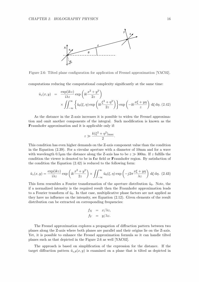
Figure 2.6: Tilted plane configuration for application of Fresnel approximation [YAC02].
computations reducing the computational complexity significantly at the same time:
uz(x, y) =exp(ikz)
iλzexp
(ik
x2 + y2
2z
)
×∫∫ ∞
−∞
{u0(ξ, η) exp
(ik
ξ2 + η2
2z
)}exp
(−ik
xξ + yη
z
)dξ dη. (2.42)
As the distance in the Z-axis increases it is possible to widen the Fresnel approxima-tion and omit another components of the integral. Such modification is known as theFraunhofer approximation and it is applicable only if:
z À k(ξ2 + η2)max
2.
This condition has even higher demands on the Z-axis component value than the conditionin the Equation (2.39). For a circular aperture with a diameter of 10mm and for a wavewith wavelength 0.5µm the distance along the Z-axis has to be z À 300m. If z fulfills thecondition the viewer is denoted to be in far field or Fraunhofer region. By satisfaction ofthe condition the Equation (2.42) is reduced to the following form:
uz(x, y) =exp(ikz)
iλzexp
(ik
x2 + y2
2z
)×
∫∫ ∞
−∞u0(ξ, η) exp
(−j2π
xξ + yη
λz
)dξ dη. (2.43)
This form resembles a Fourier transformation of the aperture distribution u0. Note, theif a normalized intensity is the required result then the Fraunhofer approximation leadsto a Fourier transform of u0. In that case, multiplicative phase factors are not applied asthey have no influence on the intensity, see Equation (2.12). Given elements of the resultdistribution can be extracted on corresponding frequencies:
fX = x/λz,
fY = y/λz.
The Fresnel approximation explores a propagation of diffraction pattern between twoplanes along the Z-axis where both planes are parallel and their origins lie on the Z-axis.Yet, it is possible to enhance the Fresnel approximation formula so it can handle tiltedplanes such as that depicted in the Figure 2.6 as well [YAC02].
The approach is based on simplification of the expression for the distance. If thetarget diffraction pattern uz,θ(x, y) is examined on a plane that is tilted as depicted in
CHAPTER 2. HOLOGRAPHY PHYSICS 17
the Figure 2.6 then the expression for the distance required for the Rayleigh-Sommerfeldintegral is:
r =[(y0 sin θ − z)2 + (x0 − x)2 + (y0 cos θ − y)2
]1/2. (2.44)
By introduction of r′ = (x2 + y2 + z2)1/2 to the Equation (2.44) a binomial expansioncan be applied. After the expansion, it is possible to omit all terms but first two similar tothe Fresnel approximation. The resulting expression is substituted to a modified Rayleigh-Sommerfeld integral:
uz,θ(x, y) = − a
iλ
∫∫
Σu0(x0, y0)
exp(ikr)r
χ(x0, y0, x, y) dx0 dy0,
where u0(x0, y0) is a source of the diffraction pattern and χ(x0, y0, x, y) is an inclinationfactor that is close to 1 if condition for the Fresnel approximation is valid. After a reorga-nization and further substitution a form is obtained that resembles the Fourier transform:
uz,θ(ξ, η) = exp(ikr′)∫∫
Σu0(x0, y0) exp
(ik
x20 + y2
0
2z
)exp [−i2π(ξx0 + ηy0)] dx0 dy0,
where ξ = x/(λr′) and η = (y cos θ+z sin θ)/(λr′). Note, that the result obtained result isrespective to a plane deformed by coordinates ξ and η and it assumes that the conditionfor the Fresnel approximation is valid.
2.6.3 Diffraction Condition and Diffraction Orders
A diffraction condition specifies a result of a diffraction of a plane wave on a thin cosinegrating [Goo05, Kra04]. The cosine grating is a thin cosine amplitude grating on a planewith a amplitude transmittance function:
tA(ξ, η) = exp[12
+m
2cos
(2π
ξ
Λξ
)]rect
(ξ
2w
)rect
( η
2w
), (2.45)
where ξ and η are coordinates on a grating, 2w is the width/height of rectangular aperture,m represents a difference between maximum and minimum of the tA, and Λξ is the gratingperiod.
If such grating is illuminated by unit amplitude plane wave then a diffraction occurs.By an application of the convolution theorem to tA it is possible to obtain the Fouriertransform of tA that can be utilized to build the Fraunhofer diffraction pattern, i.e. adiffraction pattern in the far field:
u(x, y) =a
i2λzexp
[ikz + i
k
2z(x2 + y2)
]sinc
(2wy
λz
)
×{
sinc(
2wx
λz
)+
m
2sinc
[2w
λz
(x +
λz
Λξ
)]+
m
2sinc
[2w
λz
(x− λz
Λξ
)]} (2.46)
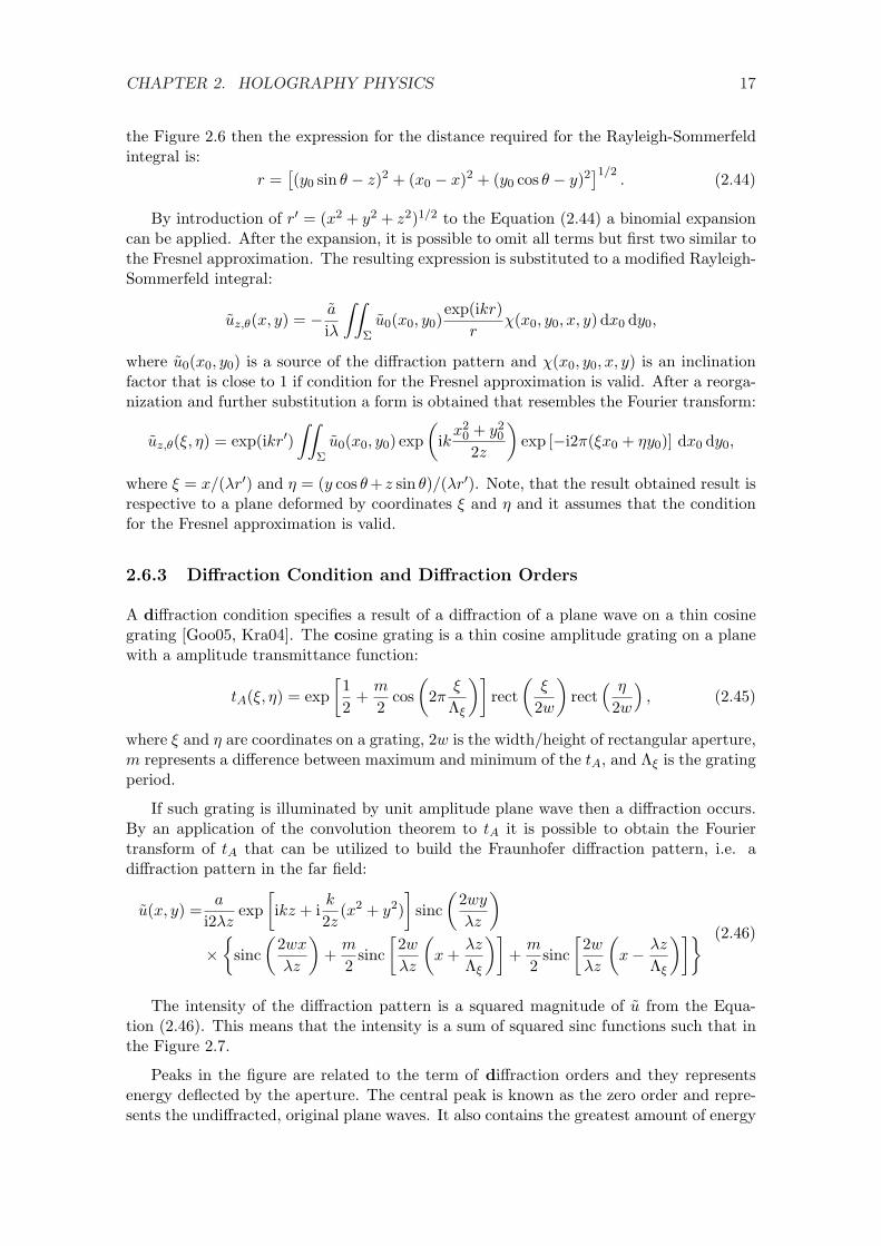
The intensity of the diffraction pattern is a squared magnitude of u from the Equa-tion (2.46). This means that the intensity is a sum of squared sinc functions such that inthe Figure 2.7.
Peaks in the figure are related to the term of diffraction orders and they representsenergy deflected by the aperture. The central peak is known as the zero order and repre-sents the undiffracted, original plane waves. It also contains the greatest amount of energy

CHAPTER 2. HOLOGRAPHY PHYSICS 18
Figure 2.7: Intensity of Fraunhofer diffraction pattern for thin amplitude cosine grat-ing [Goo05].
of the original undiffracted plane wave. The both side peaks are known as the first ordersand represents original plane waves diffracted according to the diffraction condition, seebelow.
The portion of the energy that is divided into individual diffraction orders is 12 +
m2 cos(2πΛξξ) and can be found as the squared coefficient of the delta function from theFourier transform of the amplitude modifier ta in the Equation (2.45). Note, that whilethe sinc functions in Fourier transform of the tA spreads the energy, the delta functiondetermine the power in each order. The zero order obtains 1/4 = 25.0% of the energydelivered by the incident wave, the maximum portion for the first order is 1/16 = 6.25%of the incident power; the rest is absorbed by the grating or reflected. The percentage ofthe energy for the first order is known as the diffraction efficiency of the grating.
A better diffraction efficiency of up to 33.8% has the thin sinusoidal phase grating thatemploys complex amplitude transmittance instead of the real one in the Equation (2.45).This kind grating also leads to a formation of higher orders then just only the first andthe zero ones. As the approach for derivation of diffraction order energy is similar to theamplitude grating it will not be exposed here. For more details, refer to [Goo05].
Basically, each diffraction order is the original illuminating plane wave with differentportion of energy that is propagated to a different direction. The direction of the propaga-tion for a given grating order is determined from the optical path difference of individual”rays”. The difference can be obtained at integer multiplies of λ because only in such casea planar wavefront is formed. Thus, for a transmission grating, the incoming plane waveis diffracted according to:
sin θξ2 = sin θξ1 + qλ
Λx, (2.47)
where θξ1 is an angle of the incident wave, θξ2 is an angle of the diffracted wave for givenorder q, and Λx is the period of the grating, see Figure 2.8.
2.6.4 Propagation in Angular Spectrum
The Fresnel approximation allows to compute a propagation of a wave but it has limita-tions on distance due to condition in the Equation (2.39). Even though this condition isunnecessarily strict and it is possible to apply the Fresnel approximation even for shorterdistances, still it is not applicable for a region closer to a plane with known wave distri-

CHAPTER 2. HOLOGRAPHY PHYSICS 19
Figure 2.8: Diffraction grating and diffraction condition.
bution u0 unless the third or higher components of the binomial expansion are taken intoaccount.
For shorter distances the Rayleigh-Sommerfeld diffraction integral, see the Equation (2.32),offers a solution. Unfortunately, an application of this integral leads to a unpleasant highcomputation complexity and thus renders this solution almost unusable. Yet, a slightlydifferent approach can be formulated if a Fourier transform of input wave distribution,which is also known as the angular spectrum, is considered [EO06, Goo05, TB93].
If a plane wave distribution F (kx, ky) of plane waves is known then it is possible todetermine a field u at a given point p as:
u(p) =∫∫
F (kx, ky) exp(−ik · p) dkx dky, (2.48)
where kz = (k2−k2x−k2
y)1/2. It is assumed that k2
z ≥ 0. If in any case k2z becomes negative
then kz becomes a complex number. A wave with kz ∈ C is known as the evanescent wave[BW05]. This wave is propagated as well but its amplitude decays exponentially withincreasing |z|, if it is propagated along the Z-axis5.
For a % : z = 0, the field is determined according to the following:
u0(x, y) =∫∫
F (kx, ky) exp[−i(kxx + kyy)] dkx dky. (2.49)
It can be seen in the Equation (2.49) that the plane wave distribution F is proportionalto the Fourier transform of the distribution u0 on the plane. More precisely, that F =F {u0} /(2π)2.
By a knowledge of plane wave distribution it is possible to estimate a distributionon an arbitrary distance along the Z-axis. Waves are propagated according to the Equa-tion (2.48). If the phase shift term is expanded properly then it is possible to obtain aform that resembles the Fourier transform as well6:
u(p) =∫∫ {
F (kx, ky) exp(−ikzz)}
exp[−i(kxx + kyy)] dkx dky. (2.50)
Then, computation of a field distribution u on a plane that is parallel to the source planeat the distance z along positive Z-axis can be expressed as following:
u = F−1 {F {u0} exp(−ikzz)} , (2.51)5The exponential nature of attenuation is visible from substitution of complex-valued kz to the Equa-
tion (2.48).6Note, that individual wavevector components contains 2π/λ as the length of the wavevector is the
wavenumber.

CHAPTER 2. HOLOGRAPHY PHYSICS 20
Figure 2.9: Original (left) and transformed (right) distribution of plane waves obtainedby Fourier transform.
where u is a wave distribution on a target plane while u0 is wave distribution on a sourceplane.
This approach can be further modified to handle spatial shifting in the XY-plane andtilting as well. This is achieved by an application of simple geometrical operation ofrotation stored in a form of a 3× 3 matrix R and a translation in a form of a vector b:
p′ = pR + b. (2.52)
By substitution of the expression for a point p on a target plane to the Equation (2.48)and reorganization of the result, an expression for distribution u on a target plane is:
u =1
4π2F−1
{4π2F {u0} exp[i(kR) · b]J(kz, k
′z)
}, (2.53)
where k′z is a Z-axis component of the wavevector k transformed by the matrix R andfunction J(kz, k
′z) = kz/k′z is a Jacobian correction factor. The transformation of the
wavevector k by the matrix R is equal to a shifting of a portion of hemispherical surfaceover the hemispherical surface because all possible wavevectors excluding wavevector forevanescent waves forms a hemisphere of diameter equal to a wavenumber, see Figure 2.9.
The drawback of the approach is that it is sensitive to overlapping of both target andsource plane. Due to the assumption on periodic nature of functions processed by theFourier transform a disturbance appears if the target and source plane do not overlapeach other after an orthogonal projection along the Z-axis. Yet, this can be avoided bycombining of a proper propagation as mentioned in [TB93], so that miss in overlap doesnot occur at all.
2.6.5 Propagation in Lenses
Wave that propagates through an optically dense material or a material with differentrefractive index is slowed down, i.e. a wave propagating through such material is delayed.A lens is a optically dense material of a certain geometry. For purposes of simplicity, onlya thin lens are considered. For the ray-based optics a thin lens is a lens that causes aray to exit the lens at a given point that is approximately the same as the point of entry.This means that in the case of a wave the thin lens causes only a slowdown of portions ofincoming wavefronts. The slowdown is demonstrate itself as a change in phase.

CHAPTER 2. HOLOGRAPHY PHYSICS 21
Figure 2.10: Lens and its coordinate system. Note, that the radius R2 of the right-handsurface is negative as the ray is assumed to travel from left to right [Goo05, SJ05].
The amount of the slow down can be expressed in a form of a multiplicative phasefactor [Goo05, SJ05]:
tl(x, y) = exp[ikn∆(x, y)] exp{ik[∆0 −∆(x, y)]}= exp[ik∆0] exp[ik(n− 1)∆(x, y)], (2.54)
where ∆(x, y) is a lens thickness function, ∆0 is maximum lens thickness, and n is arefraction index of the lens. Attenuation due to reflection and loss inside the lens isomitted. Note, that the factor causes a change in the phase that is equal to a sum ofthe phase changed due to the lens itself and phase change due to travel outside the lens,see Figure 2.10. The application of the factor on incident field ul leads to a field u′l thatrepresents a field immediately after the lens, i.e. u′l(x, y) = tl(x, y)ul(x, y).
The most important component of the Equation (2.54) is the thickness function ∆(x, y).This function is a sum of thicknesses ∆1, ∆2 of both curved parts and thickness ∆3 of thelens middle part:
∆(x, y) = ∆1(x, y) + ∆2(x, y) + ∆3
= (∆01 − ζ1) + (∆02 − ζ2) + ∆3. (2.55)
As it is shown in the Figure 2.10, the thickness modification for the left-hand side ofthe lens is ζ1 = R1 − (R2
1 − r2)1/2; the right-hand side is similar. Thus, according to theEquation (2.55) the thickness function is:
∆(x, y) = ∆0 −R1
[1−
(1− x2 + y2
R21
)1/2]
+ R2
[1−
(1− x2 + y2
R22
)1/2]
, (2.56)
where ∆0 = ∆01 + ∆02 + ∆3. The thickness function can be substituted to the Equa-tion (2.54) in order to form an expression for a phase delay.

CHAPTER 2. HOLOGRAPHY PHYSICS 22
Yet, the equation for the thickness is still complicated for practical use. Nevertheless,if the extent in both X- and Y-axis is sufficiently small then it is possible to consider onlyparaxial rays and apply an approximation similar to the Fresnel one:
(1− x2 + y2
R21
) 12
≈ 1− x2 + y2
2R21
.
This approximation leads to a significant simplification of the Equation (2.56) to aform that is substituted to multiplicative phase factor tl defined in the Equation (2.54)and gives:
tl(x, y) = exp(ikn∆0) exp[−ik(n− 1)
x2 + y2
2
(1
R1− 1
R2
)]. (2.57)
In a praxis the first component exp(ikn∆0) is omitted as it is constant for the whole lensand thus it is equivalent to a constant phase shift. The second component can be furthersimplified by the Lens maker equation:
1f≡ (n− 1)
(1
R1− 1
R2
), (2.58)
where f is the focal length. Focal length is a point where all parallel rays intersects afterpassing a the lens. Analogically, in wave optics it is a place where incoming wavefrontthat were modified by the lens become a infinitely small point. This is obvious fromthe Equation (2.59) when applied to a normally incident unit-amplitude plane wave. Theresulting expression is a form similar to the quadratic approximation of the spherical wave.The application of the Lens maker equation leads to a widely used expression for the phasetransformation of the lens:
tl(ξ, η) = exp(−ik
ξ2 + η2
2f
). (2.59)
The lens described by the Equation (2.59) exhibits a certain aberration in a phase.This aberration case be neglected if the intensity is the desired output. Otherwise, acorrection has to be applied. This phase correction can be determined from application ofthe Fresnel approximation and the Equation (2.59) to a field u(ξ, η) at position z = 2f infront of the lens. The field uv(x, y) at z = 2f behind the lens has to be the original fieldwith inverted coordinates [Wei], i.e. x = −ξ and y = −η. A difference between fields uand uv is eliminated by a correction factor [SJ05]:
p(x, y) = exp(−ik
x2 + y2
2f
). (2.60)
The overall equation for a setup with a source plane a(ξ, η) placed behind the thin lensof focal length f and propagated by use of a propagation kernel k(ξ, η;x, y) is:
u(x, y) =∫∫
a(ξ, η)l(ξ, η)k(ξ, η; x, y) dξ dη.
The side effect of the thin lens is its capability perform a Fourier transform in its backfocal plane. Focal plane is a plane parallel to the lens at focal distance. The configurationthat is capable of the Fourier transformation is depicted in the Figure 2.11.
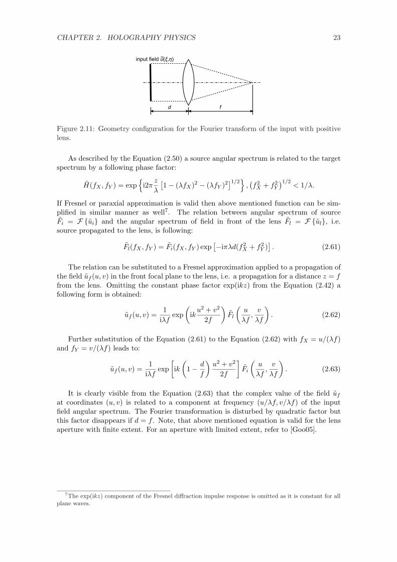
CHAPTER 2. HOLOGRAPHY PHYSICS 23
Figure 2.11: Geometry configuration for the Fourier transform of the input with positivelens.
As described by the Equation (2.50) a source angular spectrum is related to the targetspectrum by a following phase factor:
H(fX , fY ) = exp{
i2πz
λ
[1− (λfX)2 − (λfY )2
]1/2}
,(f2
X + f2Y
)1/2< 1/λ.
If Fresnel or paraxial approximation is valid then above mentioned function can be sim-plified in similar manner as well7. The relation between angular spectrum of sourceFi = F {ui} and the angular spectrum of field in front of the lens Fl = F {ul}, i.e.source propagated to the lens, is following:
Fl(fX , fY ) = Fi(fX , fY ) exp[−iπλd(f2
X + f2Y )
]. (2.61)
The relation can be substituted to a Fresnel approximation applied to a propagation ofthe field uf (u, v) in the front focal plane to the lens, i.e. a propagation for a distance z = ffrom the lens. Omitting the constant phase factor exp(ikz) from the Equation (2.42) afollowing form is obtained:
uf (u, v) =1
iλfexp
(ik
u2 + v2
2f
)Fl
(u
λf,
v
λf
). (2.62)
Further substitution of the Equation (2.61) to the Equation (2.62) with fX = u/(λf)and fY = v/(λf) leads to:
uf (u, v) =1
iλfexp
[ik
(1− d
f
)u2 + v2
2f
]Fi
(u
λf,
v
λf
). (2.63)
It is clearly visible from the Equation (2.63) that the complex value of the field uf
at coordinates (u, v) is related to a component at frequency (u/λf, v/λf) of the inputfield angular spectrum. The Fourier transformation is disturbed by quadratic factor butthis factor disappears if d = f . Note, that above mentioned equation is valid for the lensaperture with finite extent. For an aperture with limited extent, refer to [Goo05].
7The exp(ikz) component of the Fresnel diffraction impulse response is omitted as it is constant for allplane waves.

Chapter 3
Optical Holography
Optical holography stands on the physical phenomenon of diffraction described in thesection 2.5. The optical holography has one big advantage with respect to the digitalholography which is that the diffraction is performed literally with the speed of light. Itis so much not true for the numerical simulation of this phenomenon.
In this section, the principle of the optical holography is described. There are manyways of acquiring holograms so some most usual are presented. The mathematical principleof the reconstruction is provided.
3.1 Holography principle
Holography is about capturing and reproducing light filed. The light field is at eachpoint determined by an amplitude and phase. In a case of classical photography the lightfield is integrated over some time and the adequate optical intensity is captured on aphotographic material. When photograph is illuminated by a light source, the capturedintensity is replayed into all directions. That is the reason, why reproduced image looksflat, without depth.
Holography, on the contrary, is a technique which records the phase and amplitudeof the light field. When a hologram is illuminated by a proper light source, the exactamplitude and phase is reconstructed and the original light field recreated. Since theobserver has the whole light field available, the genuine three dimensional sensation isachieved.
Holography uses almost the same materials for capturing as the photography andtherefore the phase and amplitude cannot be recorded directly but rather in an encodedform, i.e. in a form of diffraction grating. The diffraction grating is formed by the fringesproduced from interference of the reference beam and the scattered beam reflected from acaptured scene. The interference fringes inflicts variation of intensity across the capturingmedium. This variation results in variation of transparency which effectively forms thewanted diffraction grating. Diffraction gratings diffracts or in other words bends light andmost fortunately, or rather because of the physics of diffraction, one component of thediffracted light field matches the initially captured one.
It is important to emphasise the fact that the reconstructed light field is part of somemore complex light field. Finding ways of separating the wanted part of diffracted light
24

CHAPTER 3. OPTICAL HOLOGRAPHY 25
b)
c)
Hologram Fotography
a)
d)
Figure 3.1: [v0.9]Difference between hologram and a common photo for a scene (a): adifference between incoming intensity from various direction for a given sample (b) and anoutgoing intensity (c) for the same sample leads to a different resulting image for a tiltedviewing screen (d).
a)
b) c)
Figure 3.2: [v0.9]The most basic principle of optical recording (b) and reconstructing (c).Note, that the reconstruction (c) generates same impression as in the case of the originalscene (a).
CHAPTER 3. OPTICAL HOLOGRAPHY 26
Hologram Hologram
Reference planar wave Reference planar wave
ObjectVirtual
image
Real
image
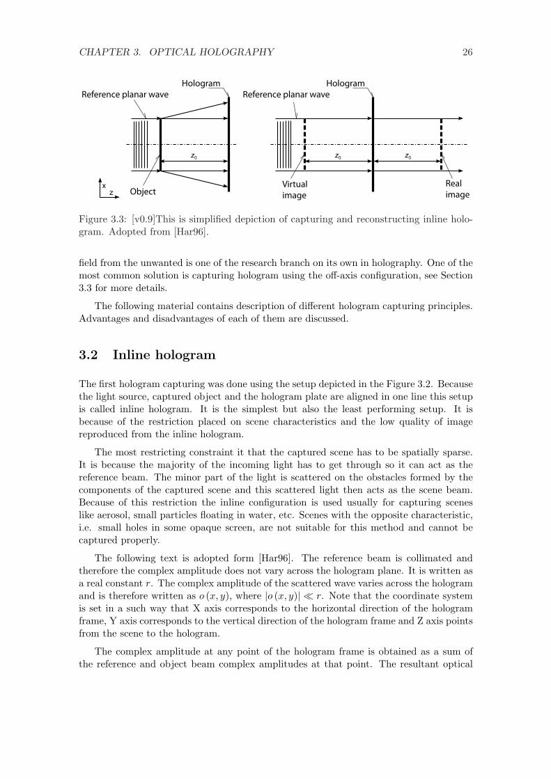
Figure 3.3: [v0.9]This is simplified depiction of capturing and reconstructing inline holo-gram. Adopted from [Har96].
field from the unwanted is one of the research branch on its own in holography. One of themost common solution is capturing hologram using the off-axis configuration, see Section3.3 for more details.
The following material contains description of different hologram capturing principles.Advantages and disadvantages of each of them are discussed.
3.2 Inline hologram
The first hologram capturing was done using the setup depicted in the Figure 3.2. Becausethe light source, captured object and the hologram plate are aligned in one line this setupis called inline hologram. It is the simplest but also the least performing setup. It isbecause of the restriction placed on scene characteristics and the low quality of imagereproduced from the inline hologram.
The most restricting constraint it that the captured scene has to be spatially sparse.It is because the majority of the incoming light has to get through so it can act as thereference beam. The minor part of the light is scattered on the obstacles formed by thecomponents of the captured scene and this scattered light then acts as the scene beam.Because of this restriction the inline configuration is used usually for capturing sceneslike aerosol, small particles floating in water, etc. Scenes with the opposite characteristic,i.e. small holes in some opaque screen, are not suitable for this method and cannot becaptured properly.
The following text is adopted form [Har96]. The reference beam is collimated andtherefore the complex amplitude does not vary across the hologram plane. It is written asa real constant r. The complex amplitude of the scattered wave varies across the hologramand is therefore written as o (x, y), where |o (x, y)| ¿ r. Note that the coordinate systemis set in a such way that X axis corresponds to the horizontal direction of the hologramframe, Y axis corresponds to the vertical direction of the hologram frame and Z axis pointsfrom the scene to the hologram.
The complex amplitude at any point of the hologram frame is obtained as a sum ofthe reference and object beam complex amplitudes at that point. The resultant optical
CHAPTER 3. OPTICAL HOLOGRAPHY 27
intensity is then obtained using Equation Equation (2.14) as
I (x, y) = |r + o (x, y)|2 ,
= r2 + |o (x, y)|2 + ro (x, y) + ro∗ (x, y) ,(3.1)
where o∗ (x, y) is the complex conjugate of o∗ (x, y).
The optical intensity is recorded on a transparency. If it is assumed that amplitudetransmittance is a linear function of the intensity then it can be written as
t = t0 + βTI, (3.2)
where t0 is a constant background transmittance, T is the exposure time, and β is aparameter determined by the photographic material. When Equation (3.1) is substitutedinto Equation (3.2) the amplitude of this transparency is
t (x, y) = t0 + βT[r2 + |o (x, y)|2 + ro (x, y) + ro∗ (x, y)
]. (3.3)
To reconstruct the captured scene, the hologram is placed on the same position asduring capturing and illuminated by the very same reference beam and the transmittedcomplex amplitude by the hologram can be then written as
u (x, y) = rt
= r(t0 + βTr2
)+ βTr |o (x, y)|2
+ βTr2o (x, y) + βTr2o∗ (x, y)
(3.4)
The expression Equation (3.4) consists of four terms. The frist of the terms r(t0 + βTr2
)
constitutes the directly transmitted beam. The second term βTr |o (x, y)|2 is extremelysmall in comparison with the others since it has been assumed initially that |o (x, y)| ¿ rand can be therefore neglected. The third term βTr2o (x, y) is, except for a constantfactor, identical with the object beam. This light field constitutes the reconstructed im-age. Since this image is located behind the transparency and the reconstructed light fieldappears to diverge from it, it is called the virtual image . The fourth term also representsthe originally captured light field except it is complex conjugate of the field. This fieldconverges to form the so called real image, which is inverted by the Z axis.
The low quality of images reproduced from inline holograms is caused by the factthat the reconstructed virtual image fully overlaps with the directly transmitted referencebeam and with the blurred real image. This fact was the reason for low interest aboutholography at the beginning. The efficient way of separating the virtual image from itsreal counterpart and from the zero order beam was developed by Leith and Upatnieks in60’ and it is introduced in the following section.
3.3 Off-axis hologram
The problem of overlapping virtual image with the real image and transmitted beam wassolved by creating more complicated setup. The source beam was divided and while onebeam was used to illuminate the captured scene which scattered it onto the hologram planeas a scene beam the second one was directed onto the hologram without modification

CHAPTER 3. OPTICAL HOLOGRAPHY 28
Figure 3.4: [v0.1]This is simplified depiction of capturing (left) and reconstructing (right)offaxis hologram. Adopted from [Har96].
and serves as the reference beam. This more complex configuration is depicted in theFigure 3.3.
The offaxis capturing principle can be described by the same formalism used in theprevious section, text is adopted form [Har96]. The complex amplitude due to the objectbeam at any point on the hologram frame can be written as
o (x, y) = |o (x, y)| exp [−iφ (x, y)] , (3.5)
while that due to the reference beam is
r (x, y) = r exp (i2πξrx) , (3.6)
where ξr = sin θ/λ. The resultant intensity at the hologram plane is
I (x, y) = |r (x, y) + o (x, y)|2
= |r (x, y)|2 + |o (x, y)|2+ r |o (x, y)| exp [−iφ (x, y)] exp (−i2πξrx)+ r |o (x, y)| exp [iφ (x, y)] exp (i2πξrx)
= r2 + |o (x, y)|2 + 2r |o (x, y)| cos [2πξrx + φ (x, y)].
(3.7)
The amplitude transmittance of the hologram can be written as
t (x, y) = t0 + βT{|o (x, y)|2+ r |o (x, y)| exp [−iφ (x, y)] exp (−i2πξrx)+ r |o (x, y)| exp [iφ (x, y)] exp (i2πξrx)}.
(3.8)
To reconstruct the image, the hologram is illuminated by the same reference beam usedfor capturing. The complex amplitude u (x, y) of the transmitted wave can be written as:
u (x, y) = r (x, y) t (x, y) ,
= u1 (x, y) + u2 (x, y) + u3 (x, y) + u4 (x, y) ,(3.9)
CHAPTER 3. OPTICAL HOLOGRAPHY 29
where
u1 (x, y) = t0 exp (i2πξrx) , (3.10)
u2 (x, y) = βTr |o (x, y)|2 exp (i2πξrx) , (3.11)
u3 (x, y) = βTr2o (x, y) , (3.12)
u4 (x, y) = βTr2o∗ (x, y) exp (i4πξrx) . (3.13)
The first term u1 (x, y) constitutes the directly transmitted reference beam attenuatedby the constant factor. The second term u2 (x, y) is responsible for some sort of halosurrounding the reference beam. The angular spread of the halo depends on the extend ofthe object. The third term u3 (x, y) is identical with the original object wave so it is thevirtual image. And finally the fourth term u4 (x, y) is the conjugate of the original objectwave so it is the real image. However, in a case of the off axis hologram, there is additionalterm exp (i4πξrx) which indicates that the conjugate wave is deflected from the Z axis atan angle approximately twice that which the reference wave makes with it.
For this reason, the real and virtual image are reconstructed at different angles fromthe directly transmitted beam and from each other. If the offset angle θ is large enough thethree will not overlap. This method therefore eliminates all the drawbacks of the Gabor’sinline hologram.
The minimum value of the offset angle θ required to ensure that each of the imagescan be observed without any interference from its twin image, as well as from the directlytransmitted beam and the halo of scattered light surrounding it, is determined by theminimum spatial carrier frequency ξr for which there is no overlap between the angularspectra of the third and fourth terms, and those of the first and second terms. Accordingto the [Har96] they will not overlap if the offset angle θ is chosen so that the spatial carrierfrequency ξr satisfies the condition
ξr ≥ 3ξmax, (3.14)
where ξmax is the highest frequency in the spatial frequency spectrum of the object beam.
The restriction on scene characteristic found in the inline hologram does not apply ina case of the off-axis hologram. More complex and interesting scenes can be captured andconsequently reconstructed. However, the off-axis configuration is more sensitive to thecoherence length of the light source. The difference of path lengths of the reference andthe scene beam must not exceed the coherence length of the light source used. Althoughthe scene can be more or less arbitrary, the problem of laser speckle still persists.
3.4 Additional hologram types
Apart from the configurations described in the Sections 3.2 and 3.3, there are several otherhologram capturing configurations. In this section these configurations are described:
• Fourier hologram
• Image hologram
• Fraunhofer hologram
CHAPTER 3. OPTICAL HOLOGRAPHY 30
3.4.1 Fourier hologram
Fourier hologram is the one in which the complex amplitudes of the waves that interfere atthe hologram are the Fourier transforms of the complex amplitudes to the original objectand reference waves. This implies an object that lies in a single plane or is of limitedthickness.
Using the same formalism used in the cases of the inline and the off-axis holograms, thelight field’s complex amplitude leaving the object plane is o (x, y), its complex amplitudeat the hologram plate located in the back focal plane of the lens and it is
O(ξ, η) = F {o(x, y)} . (3.15)
The reference beam is derived from the point source also located in the front focalplane of the lens. If δ(x + b, y) is the complex amplitude of the light field leaving thispoint source, the complex amplitude of the reference light field at the hologram plane canbe written as
R (ξ, η) = exp(−i2πξb). (3.16)
The intensity in the interference pattern produced by these two waves is, therefore,
I (ξ, η) =1 +∣∣∣O (ξ, η)
∣∣∣2+ O (ξ, η) exp (i2πξb)+
O∗ (ξ, η) exp (−i2πξb) .(3.17)
To reconstruct the image, the processed hologram is placed in the front focal plane ofthe lens and illuminated with a collimated beam of monochromatic light. If it is assumedthat this wave has unit amplitude and that the amplitude transmittance of the processedhologram is a linear function of I (ξ, η), the intensity is the interference pattern, thecomplex amplitude of the wave transmitted by the hologram is
U (ξ, η) = t0 + βTI (ξ, η) . (3.18)
The complex amplitude in the back focal plane of the lens is then the Fourier transformof U (ξ, η),
u (x, y) = F{
U (ξ, η)}
,
= (t0 + βT ) δ (x, y) + βT o (x, y) ? o (x, y) ,
+ βT o (x− b, y) + βT o∗ (−x + b,−y) .
(3.19)
The wave corresponding to the first term on the right-hand side of equation comes to afocus on the axis, while the other that corresponds to a second term forms a halo around it.The third term produces an image of the original object, shifted downwards by a distanceb, while the fourth term gives rise to a conjugate image, inverted and shifted upwards bythe same distance b. Both images are real and can be recorded on a photographic filmplaced in the back focal plane of the lens. Since the film records the intensity distributionin the image, the conjugate image can identified only by the fact that it is inverted. Moredetails can be found in [Har96].
CHAPTER 3. OPTICAL HOLOGRAPHY 31
3.4.2 Image holograms
Image holograms are special in the way they record the images and can be considered as asecond step in creating a hologram. Instead of direct recording of the object, a previouslyhologram is used. The real image produced by that hologram is recorded through lens.The hologram plate then can be positioned in such manner that the image of the objectstraddles the plate. In such case the reconstructed image is formed in the same positionwith respect to the hologram, so a part of the image appears to be in front of the hologramand the remainder is behind it.
Image holograms are reconstructible by use of a source of appreciable size and spectralbandwidth and will still produce an acceptably sharp image. They have also increasedluminosity. However, the viewing angles are limited by the aperture of the imaging lens.More details about image holograms can be found in [Har96].
3.4.3 Fraunhofer hologram
Fraunhofer holograms are special case of the inline holograms. This class of hologramsimpose further constraint onto the scene configuration. In this case, the captured scene hasto be small enough for its Fraunhofer diffraction pattern to be formed on the photographicplate. The object is small enough if its distance z0 and lateral dimensions x0 and y0 satisfiesthe far-field condition:
z0 À(x2
0 + y20
)/λ. (3.20)
When such Fraunhofer hologram is illuminated the light contributing to the conjugateimage is spread over a large area in the plane of the primary image. This causes a conjugateimage to form only weak uniform background instead of disturbing noise. As a result, theprimary image can be viewed without significant interference from its conjugate. Moredetails can be found in [Har96].
3.5 Final notes
The optical holography is widely used in many areas. In the context of this work, themost interesting is object capturing and reconstructing for display purposes. In this area,optical holography has many advantages and also many limitations. Among the advantagesbelongs the speed and accuracy of capturing. Among disadvantages belongs unnaturalillumination produced by the coherent monochromatic light produced by lasers.
For practical display purpose, the digital medium is more suitable. It has again manyadvantages and many disadvantages. Among the advantages belongs the universality ofthe digital medium. Also the synthesis process can neglect some restriction imposed on thecaptured scene by the physical matter of the problem. The disadvantages are immaturityof the hardware and high computation demands of the synthesis process. This workaddress the former disadvantage.

Chapter 4
Digital Holography
Holography is widely used in many areas for various purposes. It is not surprising thattheir digitalised variation appeared quite early. The digitalisation brought the possibilityof computer processing but also brought the sampling based nuisances like aliasing. Therecan be identified three major areas of holography that are usually addressed in a contextof digital holography. They are the capturing, the reproduction and hologram fringessynthesis. Furthermore, digital holography introduces one specific issue, that don’t haveparallel in optical holography. The area is numerical reconstruction.
4.1 Digital capturing
Electronic devices for capturing light intensity are known for some time. The advent ofdigital cameras that begun in 90’ helped to evolve this area into cutting edge technology.The sensor arrays have as much as tens millions of sensor elements. However, the resolutionis fine but the density more important for holography. The pitch between two sensorsdirectly influences the frequencies that can be captured and large frequencies capturedmeans better hologram.
4.2 Digital reproduction
The reproduction is more interesting but less completed area. The wavefront of the inci-dent reference beam has to be modulated according to the hologram recording. This isdone by the spatial light modulator or SLM. Such devices are capable of change phaseof the light wavefront. If hologram is used as the input for SLM, the recorded sceneis reconstructed. There are numerous technologies that are used to make SLM’s work.The most important property of each SLM is again spatial density of the individual ele-ments. For holography purposes the appropriate size of such element is measured in onesof micrometres 10−6m which is quite technological challenge.
32

CHAPTER 4. DIGITAL HOLOGRAPHY 33
4.3 Hologram Synthesis
The synthesis of a hologram by a computer is vital for holographic display technology.It is also clear that such synthesis should be performed in a real time so that interactivework would be possible. Waiting even for several seconds for cursor position update isunbearable. This requirement is in contradiction with the computational requirementsof the diffraction phenomenon simulation. This contradiction can be resolved either byemploying massive computational power which is perfectly reasonable as proved by thecontemporary GPU’s, or by reducing the complexity significantly which is a preferred wayin computer science.
The complexity of the synthesis could be illustrated by the following example. Let thetarget holographic display is a planar display similar to the 17” LCD. Usual resolution of17” LCD is 1280×1024 so the pitch between pixels is 0.25 mm. A computer has to compute1.3× 106 samples if whole image is refreshed. The holographic display with 1.0 µm pitchbetween elements has resolution 320000×256000 so a computer has to compute 8.2×10¹⁰
samples if whole image is refreshed. That is 62500 times more samples in comparison tothe LCD. It should be also noted that the minimal frame rate for interactive work is 15fps so the hologram has to be computed under 60 ms and finally, the data stream for suchframe rate is 1.2 TB per second.
The specifications in the previous paragraph are, of course, the final goal specifications.For the practical experiments more coarse parameters suffice. Moreover, there is no suchholographic device in the world, that has such parameters. The holograms computed forthis work have sizes measured in centimetres and usual pitch between samples is 10 µm.
The most straightforward method of the hologram synthesis is to compute light fielddue to the intended scene content and then the hologram is computed by adding the ref-erence beam. The light field could be computed by numerical simulation of the diffractionphenomenon according to one of the diffraction models introduced in the section 2.5. It isfairly easy to do if the scene consists of planar object parallel to the hologram plane. Thelight field due to this object is computed using the Fourier transform. The complicationsarise if scene contains three dimensional object.
The simplest hologram is a hologram of a single point source of uniform sphericalwaves. Spherical waves are governed by the equation Equation (2.25). For each point atthe hologram, distance r to the point source is computed and the equation Equation (2.25)is evaluated. If scene contains more points, then the complex amplitude obtained fromthe equation Equation (2.25) for each point is accumulated and the final value constitutesthe final complex amplitude. This point source based hologram computation gave a birthto the raytracing methods.
The basis of the raytracing method is to cast rays from each sample point on a hologramframe in a uniform way into the scene. Rays that intersects the objects of a scene areevaluated as a contribution from a point source and the result is accumulated so afterevaluating all rays, the final value is obtained. This is sort of reversal of the methoddescribed in the previous paragraph.
The next possible solution is to decompose the scene contents onto simple primitives.The diffraction pattern of the primitives can be computed analytically and the final lightfield is obtained by accumulating the contributions from all primitives. This method hasseveral unsolved problems. They are surface intensity variation and occlusion.

CHAPTER 4. DIGITAL HOLOGRAPHY 34
The last known approach to the hologram synthesis is frequency based. Under someconvenient conditions, the light field can be obtained from Fourier transform. Thesemethods are fastest but they suffer from similar drawbacks as the pattern based methods.The most significant problem is occlusion.
4.4 Hologram Reconstruction
The hologram reconstruction is a process that leads to computation of wave distributionover an arbitrary surface according to a given diffraction pattern. The diffraction patternis a result of an interaction between the reconstruction wave and a hologram, where thehologram modulates the reconstruction wave, see Section 3.
4.4.1 Diffraction pattern reconstruction
If both source and target surface are parallel or tilted planes then the wave propagation isa direct application of relations described in the Section 2.6. If an approach that is basedon angular spectrum propagation is applied a loss of information occurs for tiled planes.The loss is caused by the transformation of the spectrum according to the transformationmatrix so that the target frequency is falls outside the range of the target spectrum andthus it is clipped.
The occurrence of the loss depends on both angle of rotation and sampling step. Fora discrete diffraction patterns with sampling step greater than λ/2 is the probabilityhigher [TB93]. In such case a shifting of a central frequency is assumed solution. Forexample, if the transformation is a plain rotation around the X-axis then the center (0, 0)of the source plane is actually mapped to a frequency (β/λ, 0), where β is related to acosine of the rotation angle.
In order to avoid the loss due to clip of frequencies a center is shifted to (β/λ, 0) on thetarget plane. As all operations of propagation takes place in angular spectrum, the shiftingof the center can be applied many times without a degradation cause by the clipping. Onthe other hand a degradation may occur as the target–source frequency back-mappingrequires a sample that is positioned between two known samples and thus it has to beestimated. Even a bilinear interpolation can be utilized with reasonable results [TB93].
An arbitrary target or source geometry is an arbitrary surface described by a functionthen relations are complication introducing non-linearities as the source/target coordinatesare expressed as functions [Ros99]. Such non-linearities causes inability to apply Fouriertransform for improving of the computational complexity and thus a full approximationof the integral by the summation is required. If a given direction retains a linear naturethen the Fourier transform may be utilized in its 1D form.
4.4.2 Retrieval of Phase and/or Amplitude
Hologram is an encoded form of wave distribution on a given surface such as the plane. Ifa diffraction pattern propagation is applied to the hologram after the reference wave thenthe wave proportional to the original scene wave is recreated. Besides that, also othercomponents are recreated as well. Yet, in some cases only the original scene wave is thedesirable result and such result can be extracted from the hologram numerically.
CHAPTER 4. DIGITAL HOLOGRAPHY 35
From the computational point of view, the information about the original scene en-coded inside the intensity of the hologram can be extracted by two major approaches: onebased on a phase-shift and second base on a solution of equation set for a small neighbor-hood. The phase-shift approach utilizes a set holograms of the same scene with a phaseshifted by a fraction of the wavelength [YZ97]. It can be shown that if phase shifts areselected properly an accurate estimation of u, i.e. phase and amplitude, of the scene isequivalent to equation set solution.
Phase-shift methods offers a reasonable accuracy but requires a set of holograms tobe created. The slightly different approach that is still capable to reasonable result hasno such requirement but it assumes a certain conditions [LBU04]. It assumes an off-axishologram and that in a small, approximately 3× 3 neighborhood, there is no variation ofphase and amplitude in the scene wave distribution at the hologram. By the knowledgeof the recording wave it is able to express intensities at members of the neighborhood asa non-linear set of equations. Such set can be transformed to a set of linear equations byapplication of weights based on B-spline.
Bibliography
[BW05] M. Born and E. Wolf. Principles of Optics. Cambridge University Press, 7th edition,2005.
[EO06] G.B. Esmer and L. Onural. Computation of holographic patterns between tilted planes.In Holography 2005, volume 6252, page 62521K. SPIE, 2006.
[Gab49] D. Gabor. Microscopy by reconstructed wavefronts. 1949.
[Goo05] J.W Goodman. Introduction to Fourier Optics. Roberts & Company Publishers, 3rdedition, 2005.
[Gra03] J.R. Graham. Wave optics. WWW http://grus.berkeley.edu/ jrg/ScalarWave/, 2003.
[Har96] P. Hariharan. Optical Holography: Principles, techniques and applications. CambridgeUniversity Press, 2nd edition, 1996.
[Kra04] F. Krausz. Photonics: Lecture notes, 2004.
[LBL02] D.R. Luke, J.V. Burke, and R.G. Lyon. Optical Wavefront Reconstruction: Theoryand Numerical Methods’. SIAM Review, 44:169–224, 2002.
[LBU04] M. Liebling, T. Blu, and M. Unser. Complex-wave retrieval from a single off-axishologram. J. Opt. Soc. Am. A, 21(3):367–377, 2004.
[Luc94] M. Lucente. Diffraction-Specific Fringe Computation for Electro-Holography. PhDthesis, MIT, 1994.
[Mie02] K.D. Mielenz. Optical diffraction in close proximity to plane apertures. i. boundary-value solutions for circular apertures and slits. J. res. Natl. Inst. Stand. Technol.,107(4):335–362, 2002.
[MNF+02] O. Matoba, T. J. Naughton, Y. Frauel, N. Bertaux, and B. Javidi. Three-dimensionalobject reconstruction using phase-only information from a digital hologram. In Three-Dimensional TV, Video, and Display., volume 4864, pages 122–128. SPIE, 2002.
[Ros99] J. Rosen. Computer-generated holograms of images reconstructed on curved surfaces.Appl. Opt., 38(29):6136–6140, 1999.
[SJ05] U. Schnars and W. Juepner. Optical Holography: Principles, techniques and applica-tions. Springer, 2005.
[TB93] T. Tommasi and B. Bianco. Computer-generated holograms of tilted planes by a spatialfrequency approach. Journal of the Optical Society of America A, 10:299–305, February1993.
[Wei] E. Weisstein. World of science. WWW http://scienceworld.wolfram.com/.
[YAC02] L. Yu, Y. An, and L. Cai. Numerical reconstruction of digital holograms with variableviewing angles. Optics Express, 10:1250–+, 2002.
[YZ97] I. Yamaguchi and T. Zhang. Numerical reconstruction of digital holograms with vari-able viewing angles. Optical Letters, 22(16):1268–1270, 1997.
36

List of Figures
2.1 Interference of waves . . . . . . . . . . . . . . . . . . . . . . . . . . . . . . . 5
2.2 A configuration of exploring the coherence . . . . . . . . . . . . . . . . . . . 6
2.3 Spherical wavefront deformation with increasing distance . . . . . . . . . . 9
2.4 Huygens principle . . . . . . . . . . . . . . . . . . . . . . . . . . . . . . . . . 10
2.5 Configuration of the Fresnel/Fraunhofer approximation . . . . . . . . . . . 15
2.6 Titled plane and Fresnel approximation . . . . . . . . . . . . . . . . . . . . 16
2.7 Intensity of Fraunhofer diffraction . . . . . . . . . . . . . . . . . . . . . . . 18
2.8 Diffraction grating and diffraction condition . . . . . . . . . . . . . . . . . . 19
2.9 Plane wave transformation for titled planes . . . . . . . . . . . . . . . . . . 20
2.10 Lens and its coordinate system . . . . . . . . . . . . . . . . . . . . . . . . . 21
2.11 Lens and Fourier transform . . . . . . . . . . . . . . . . . . . . . . . . . . . 23
3.1 Difference between holography and photography . . . . . . . . . . . . . . . 25
3.2 Optical hologram recording/reconstruction setup . . . . . . . . . . . . . . . 25
3.3 Inline holography setup . . . . . . . . . . . . . . . . . . . . . . . . . . . . . 26
3.4 Offaxis holography setup . . . . . . . . . . . . . . . . . . . . . . . . . . . . . 28
37

List of Tables
38