Histograms – Chapter 4

Continued

ImageJ – from last time…• Open snake.png (download from my web site)• Select Analyze/Histogram

– This is the histogram of the luminance channel of the color image

• Select Image/Color/Split Channels– You now have the red/green/blue channels individually

• Create histograms of each of these• Comment on exposure, contrast, dynamic range• Pull other images from wherever, play with it

Effects of JPEG compression• Original, uncompressed file• 229K bytes• Smooth histogram

Effects of JPEG compression• JPEG compressed file• 33K bytes• Smooth histogram – not much change, image visually lossless

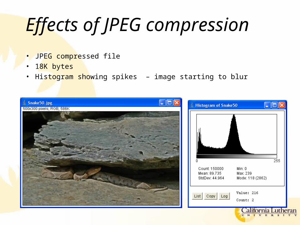
Effects of JPEG compression• JPEG compressed file• 18K bytes• Histogram showing spikes – image starting to blur

Effects of JPEG compression• JPEG compressed file• 12K bytes• Histogram showing spikes – image more blurring

Effects of JPEG compression• JPEG compressed file• 6K bytes• Histogram showing tall spikes – image blocking, color fidelity lost

Effects of JPEG compression• JPEG compressed file• 5K bytes• Histogram showing tall spikes – image blocking, color fidelity lost

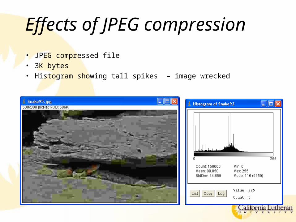
Effects of JPEG compression• JPEG compressed file• 3K bytes• Histogram showing tall spikes – image wrecked

Effects of JPEG compression• JPEG compressed file• 3K bytes• Histogram showing tall spikes and gaps – image wrecked

Effects of JPEG compression• JPEG compressed file• 2K bytes• Histogram showing tall spikes and gaps – image, what snake?

ImageJ JPEG

• Edit->Options->Input/Output…– Allows you to set level of compression– Smaller number gives more compression

at the cost of greater information loss– Larger number retains more information at

the cost of less compression

Effects of saturation

• Ideally the sensor’s range (detectable light levels from dark to bright) is greater than that of the scene being imaged

• Realistically, this doesn’t always happen• The human visual system has incredible

dynamic range due to the distribution of rods and cones in the retina

• Very difficult to match in silicon

Human visual system

• Cones: process color (3 types)• Primarily in the foveal region of the retina

• Rods: process shades of gray• Primarily in the peripheral region of the retina

Effects of saturation

• Original, looks decent enough• Histogram is smooth, contrast is a little low, exposure a little low,

dynamic range a little low

Effects of saturation

• We brighten it up by multiplying pixels by some specified values (artificially brighten it to compensate for the sensor deficiencies)

• Histogram shows dynamic range is good, contrast is good, but we get spikes and a lot of saturated pixels

Playing detective

• When you see stuff like this in the histogram, you know something is awry

• If you see spikes, either the imaging device was bad or the image was digitally manipulated• Analog pixels don’t do this

• Ditto if you see gaps• If you see a lot of saturation

either the photographer screwed up or the image was digitally manipulated (or the scene was too bright for the camera)

Computing histograms

• Because you should at least see the code…

int Histogram[] = new int[256]; // 8 bit histogram

for (int i = 0; i < imageHeight; i++) {for (int j = 0; j < imageWidth; j++) {++Histogram[image[i][j]];

}}

Computing histograms

• There may be times when your histogram is bigger than your memory size– Large bit-depth images– Floating point images

• All is not lost, we just resort to binning– In this case a single histogram entry represents a range of

pixel values [rather than a single value]– Be careful when reading these as spikes/gaps could be

hidden in the representation

Computing histograms

• Histograms of color images create another situation to be dealt with

• Color images are typically 24-bits– 8-bits each for Red, Green, and Blue– Results in 224 = 16777216 pixel values– Not suitable for direct histogram creation and binning makes

not sense – why?• There is not natural ordering of the colors as there is in a gray scale

image

– Two choices• Display the luminance histogram (the brightness content of the image)• Display the red, green, and blue histograms separately

Color histograms

Luminance Red Green Blue

Color histograms

• The green histogram will [typically] look similar to the luminance histogram

• If the red, green, and blue histograms look similar the image has most likely been white balanced– Two of the channels (e.g. red, and blue) have been

enhanced (contrast, dynamic range) to look similar to the third (e.g. green)

– This “trick” is performed to make sure that white objects in the scene appear white in the resulting image

– Corrects for deficiencies in the imaging device

Color histograms

• Another option is to create a three dimensional histogram or scatter plot of the image pixel colors

Cumulative histogram

• A bin in the cumulative histogram is the sum of all lower bins of the “normal” histogram

• It’s not overly useful for analysis but will provide some needed information for certain image enhancement operations

KijhistogramiHcumulativei

j

0)()(0

Cumulative histogram

Cumulative histogram

• I’ve placed a plugin for the cumulative histogram on the website

• Download it and drop it into the folder

• It will show up under the Plugins->Chapter04 menu

C:\Program Files\ImageJ\plugins\Chapter04