Highly efficient Machine learning for HoloLens

Andrew Fitzgibbon, Microsoft

@awfidius

2

3

4

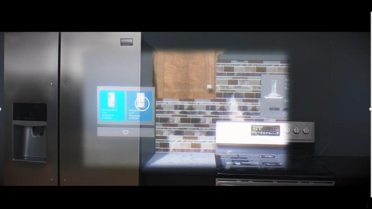
APPLICATIONS

OF HOLOLENS

Deskless workers

Merge real and digital world

3D designers / decision makers /

learners

Create and communicate 3D concepts in 3D

Everyone…

TASK WORKER

3D LEARNING

/ MEDICAL

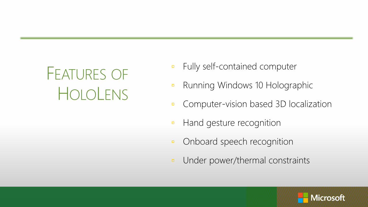
FEATURES OF

HOLOLENS

Fully self-contained computer

Running Windows 10 Holographic

Computer-vision based 3D localization

Hand gesture recognition

Onboard speech recognition

Under power/thermal constraints

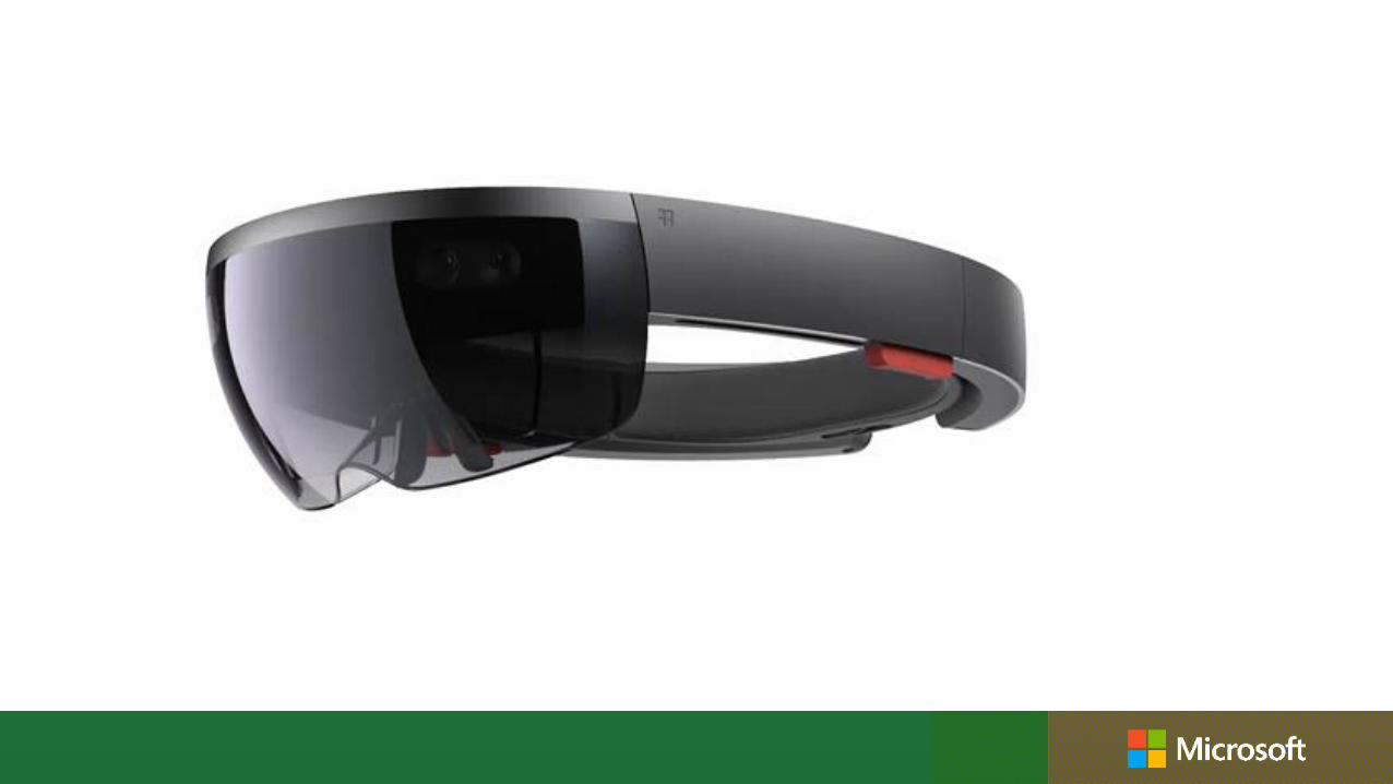
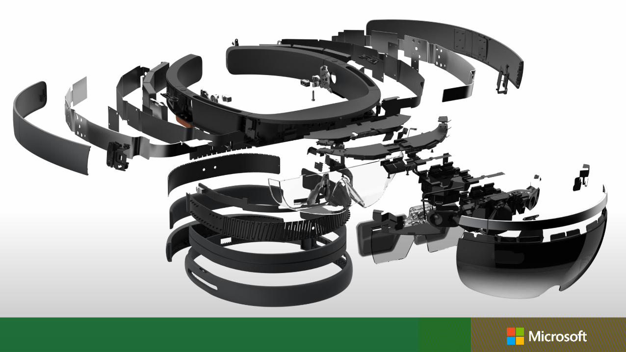
AN INTRODUCTION TO HOLOLENS

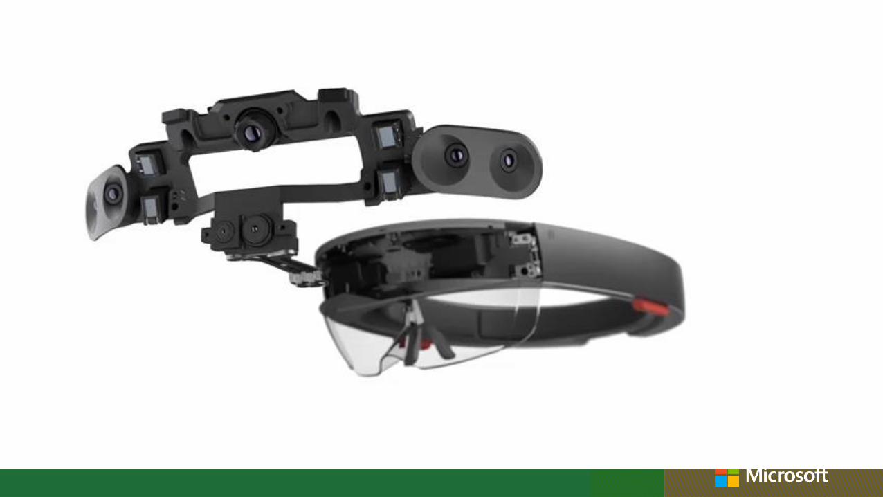
HARDWARE

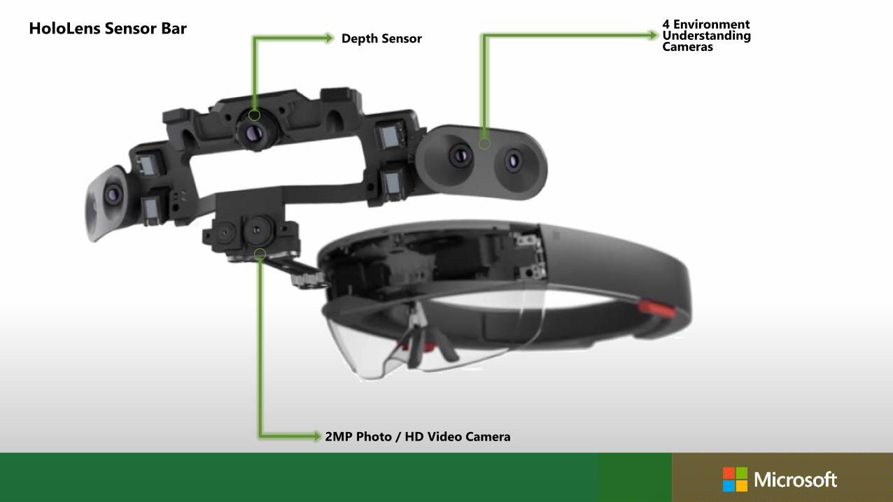
4 Environment Understanding Cameras

HoloLens Sensor BarDepth Sensor

2MP Photo / HD Video Camera

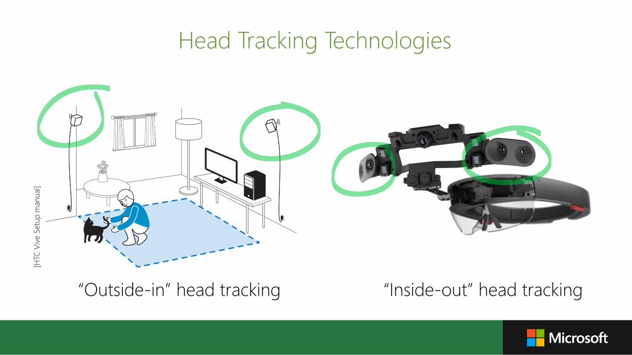
Head Tracking Technologies

“Outside-in” head tracking

[HTC

Viv

eSetu

p m

anual]

“Inside-out” head tracking

15

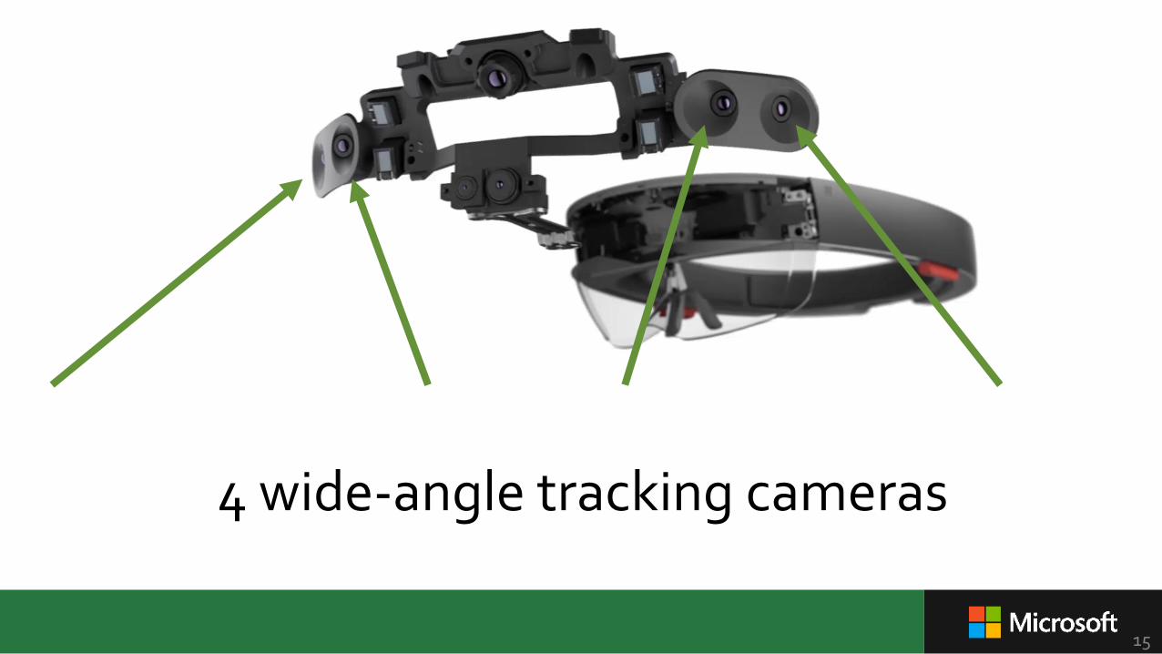
4 wide-angle tracking cameras

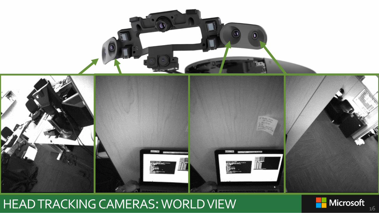
HEADTRACKING CAMERAS: WORLDVIEW 16

4 wide-angle tracking cameras

4 Environment Understanding Cameras

HoloLens Sensor BarDepth Sensor

2MP Photo / HD Video Camera

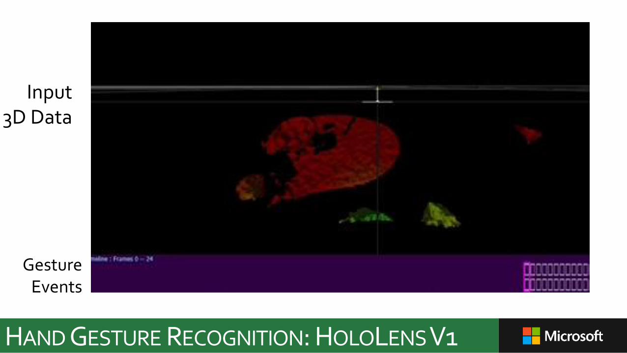
Input3D Data

GestureEvents

HAND GESTURE RECOGNITION: HOLOLENSV1

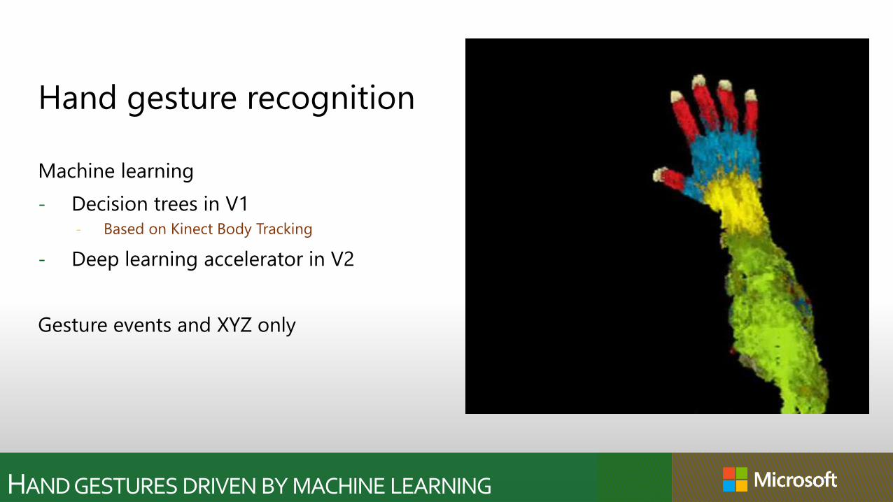
HAND GESTURES DRIVEN BY MACHINE LEARNING

Hand gesture recognition

Machine learning

- Decision trees in V1- Based on Kinect Body Tracking

- Deep learning accelerator in V2

Gesture events and XYZ only

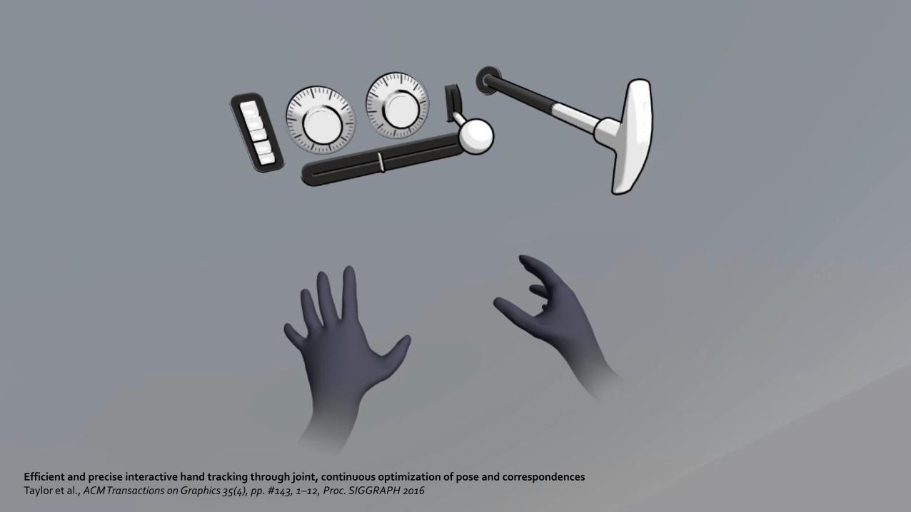
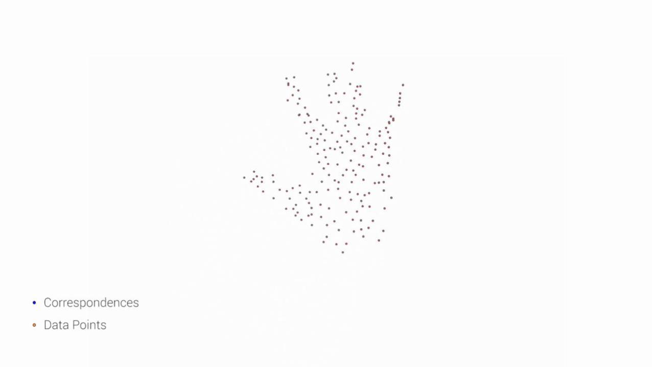
Efficient and precise interactive hand tracking through joint, continuous optimization of pose and correspondences Taylor et al., ACM Transactions on Graphics 35(4), pp. #143, 1–12, Proc. SIGGRAPH 2016

4 Environment Understanding Cameras

HoloLens Sensor BarDepth Sensor

2MP Photo / HD Video Camera

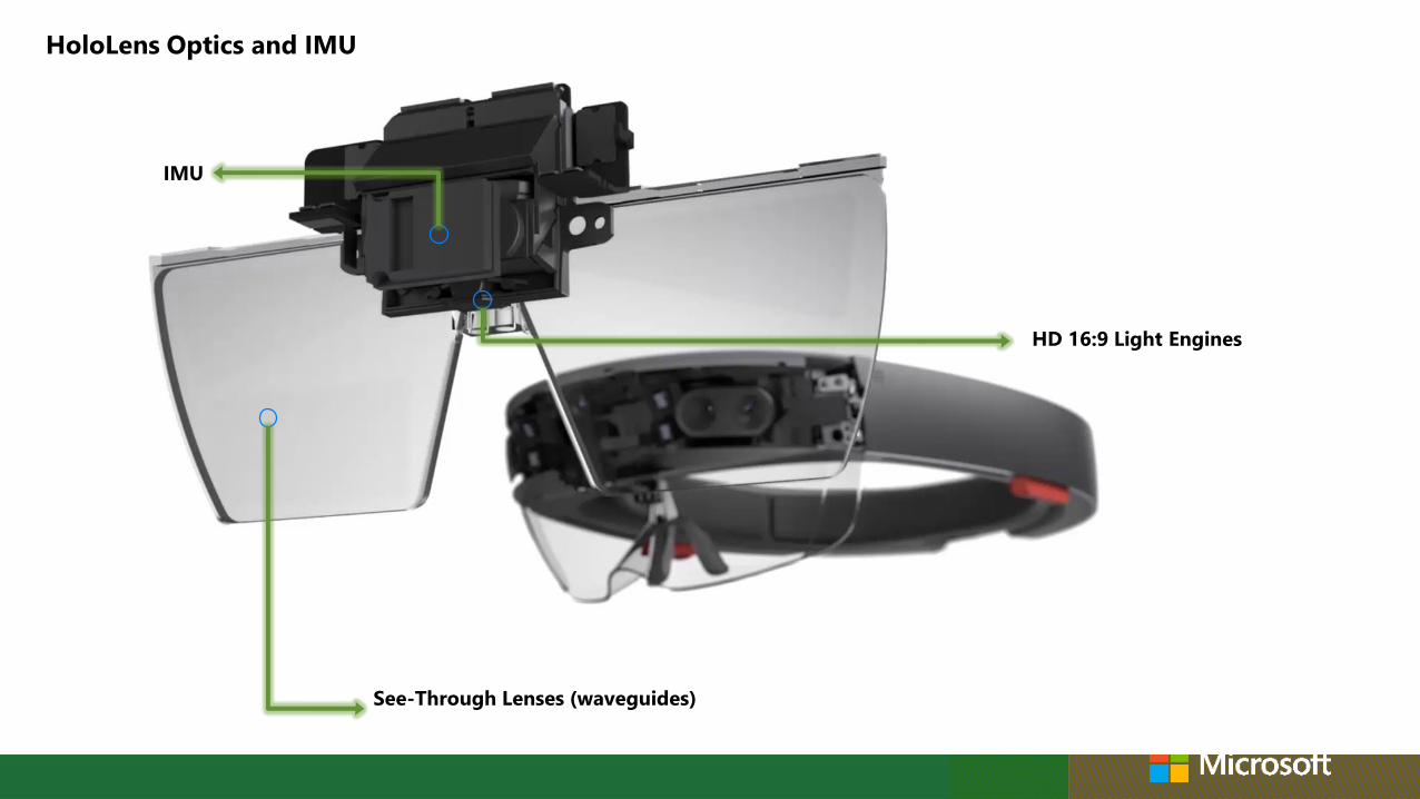
See-Through Lenses (waveguides)

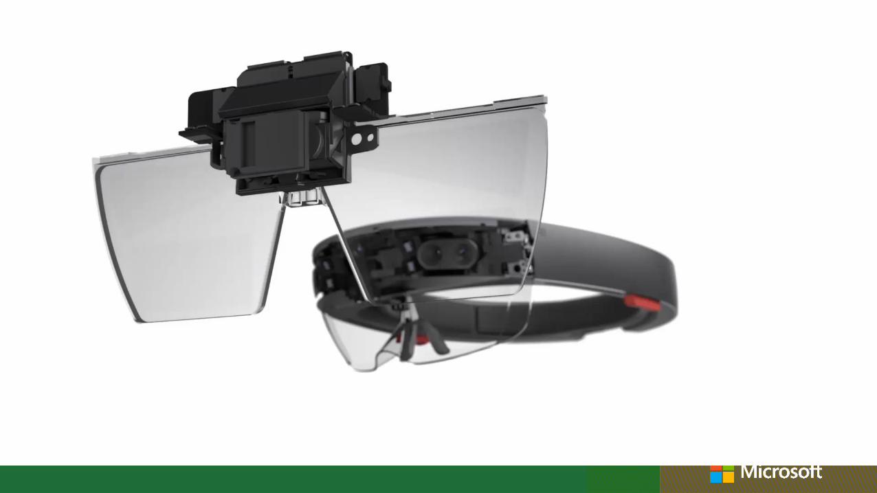
HoloLens Optics and IMU

HD 16:9 Light Engines

IMU

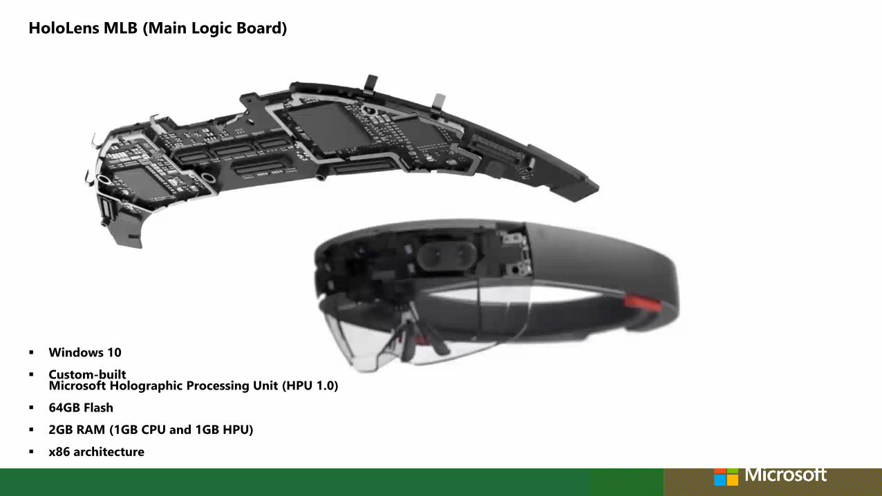
HoloLens MLB (Main Logic Board)

▪ Windows 10

▪ Custom-built Microsoft Holographic Processing Unit (HPU 1.0)

▪ 64GB Flash

▪ 2GB RAM (1GB CPU and 1GB HPU)

▪ x86 architecture

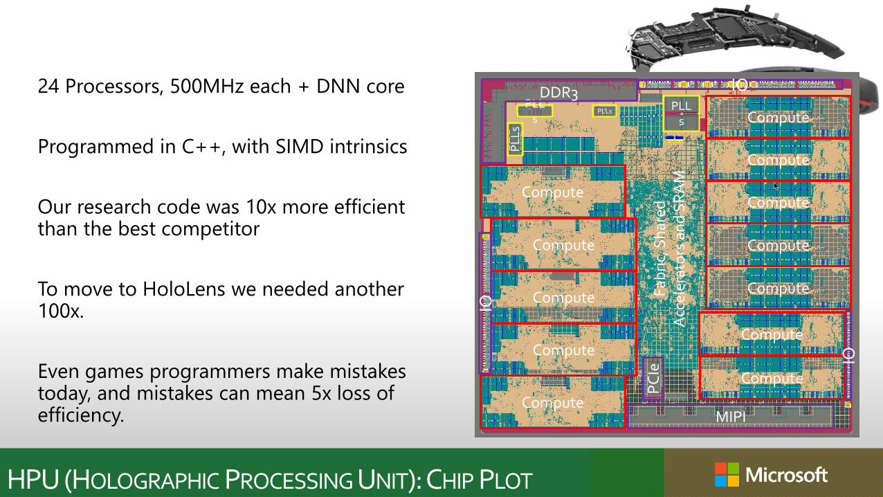
HPU (HOLOGRAPHIC PROCESSING UNIT): CHIP PLOT

24 Processors, 500MHz each + DNN core

Programmed in C++, with SIMD intrinsics

Our research code was 10x more efficient than the best competitor

To move to HoloLens we needed another 100x.

Even games programmers make mistakes today, and mistakes can mean 5x loss of efficiency.

Compute

Compute

Compute

Compute

Compute

Compute

Compute

Compute

Compute

Compute

Compute

Compute

PLLs

PLLs

PLLs

PL

Ls

DDR3

MIPI

PC

Ie

IO

IO

IO

Fab

ric,

Sh

ared

A

ccel

erat

ors

an

d S

RA

M

HoloLens Spatial Sound

also 4 microphones for speech/beamforming

EFFICIENT COMPUTER VISION & ML:Learning + Model fitting

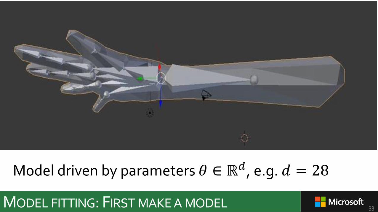
MODEL FITTING: FIRST MAKE A MODEL 33

Model driven by parameters 𝜃 ∈ ℝ𝑑, e.g. 𝑑 = 28

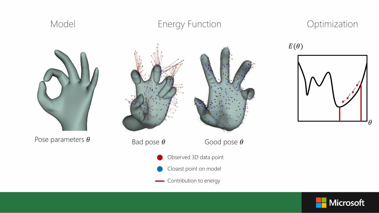
Energy Function

Observed 3D data point

Closest point on model

Bad pose 𝜃 Good pose 𝜃

Contribution to energy

Model Optimization

Pose parameters 𝜃

𝜃

𝐸(𝜃)

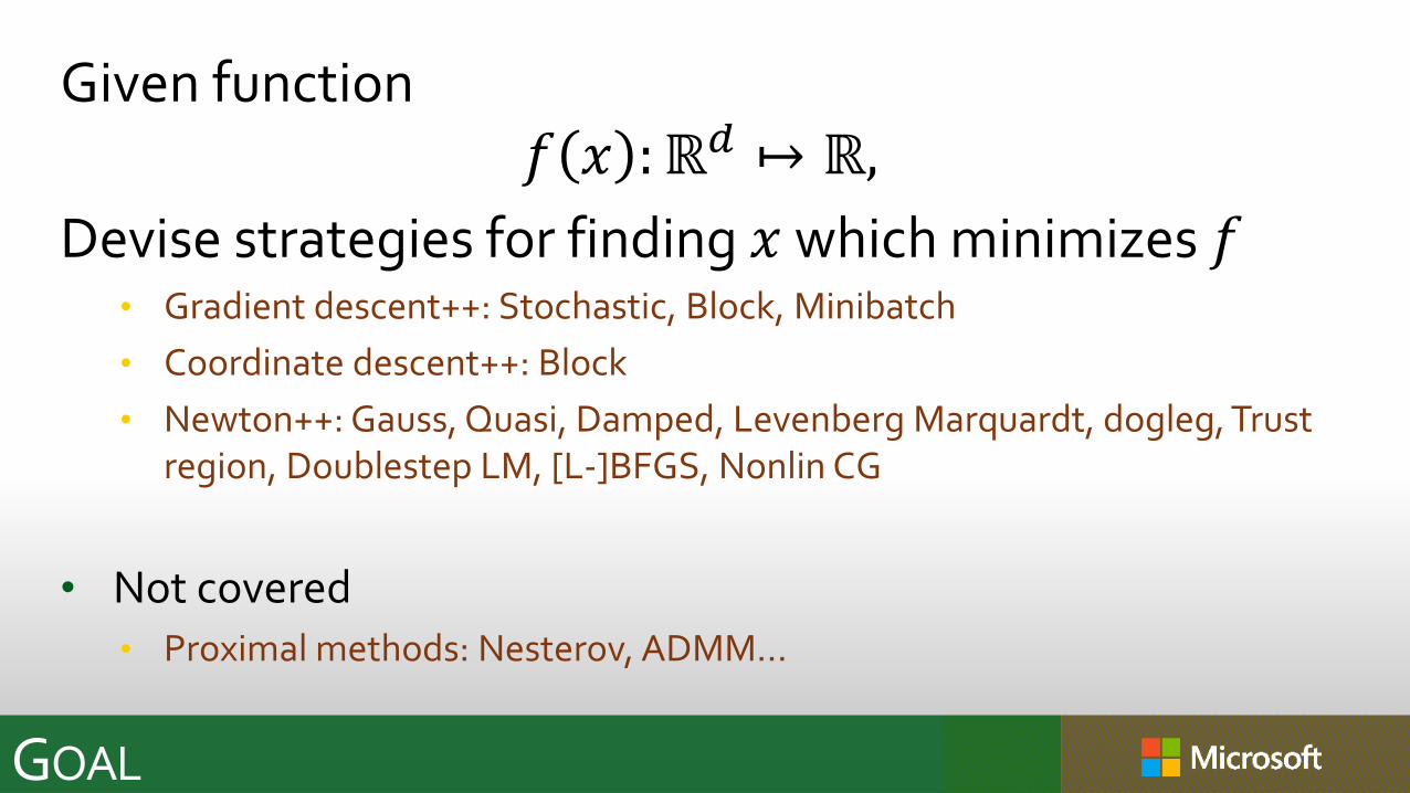
GOAL

Given function𝑓 𝑥 :ℝ𝑑 ↦ ℝ,

Devise strategies for finding 𝑥 which minimizes 𝑓• Gradient descent++: Stochastic, Block, Minibatch

• Coordinate descent++: Block

• Newton++: Gauss, Quasi, Damped, Levenberg Marquardt, dogleg, Trust region, Doublestep LM, [L-]BFGS, Nonlin CG

• Not covered• Proximal methods: Nesterov, ADMM…

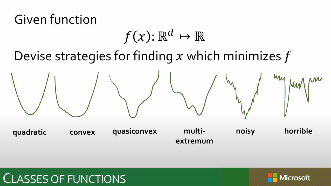
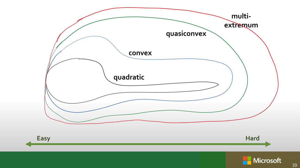
CLASSES OF FUNCTIONS

quadratic convex quasiconvex multi-extremum

noisy horrible

Given function𝑓 𝑥 :ℝ𝑑 ↦ ℝ

Devise strategies for finding 𝑥 which minimizes 𝑓

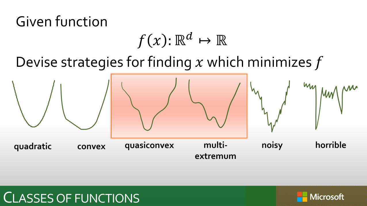
CLASSES OF FUNCTIONS

quadratic convex quasiconvex multi-extremum

noisy horrible

Given function𝑓 𝑥 :ℝ𝑑 ↦ ℝ

Devise strategies for finding 𝑥 which minimizes 𝑓

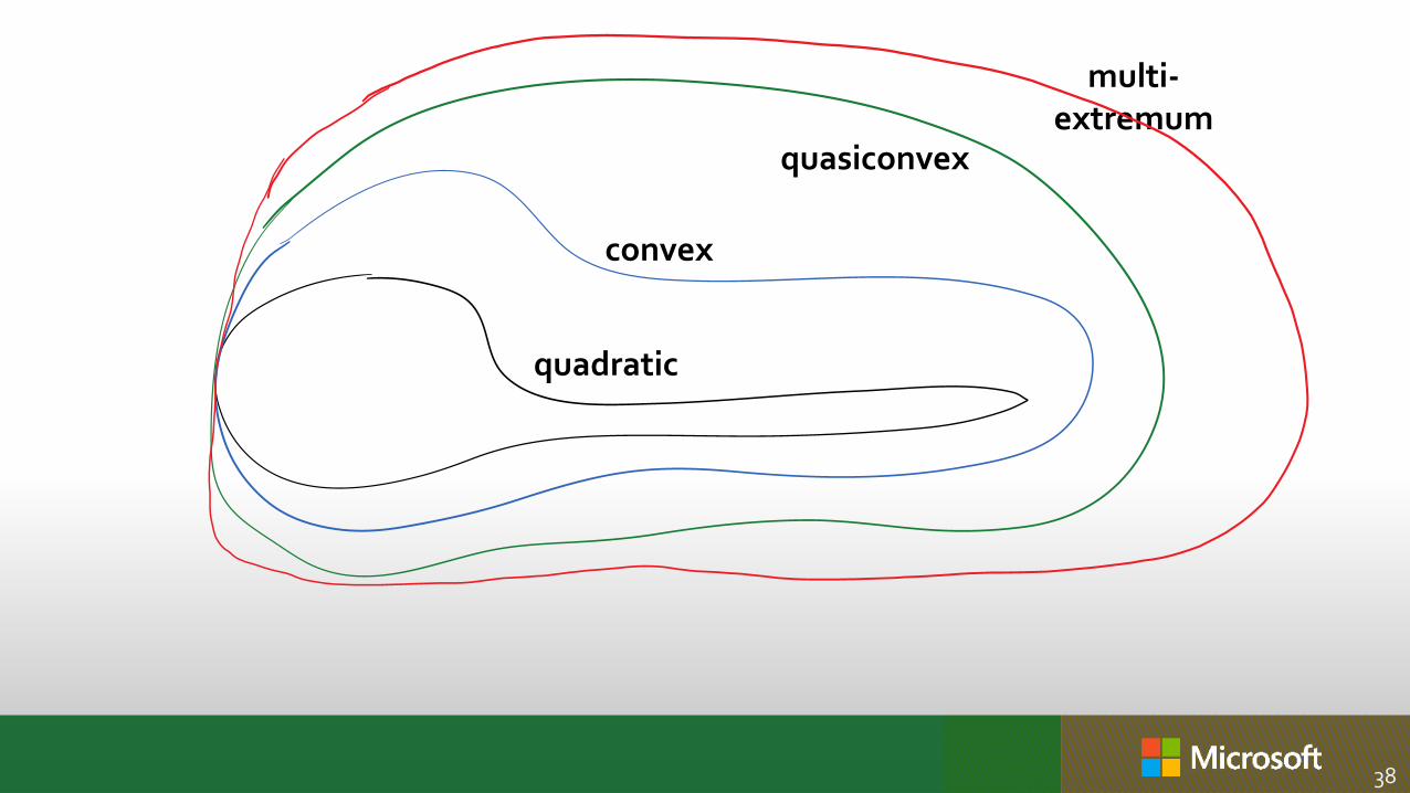
38

quadratic

convex

quasiconvex

multi-extremum

39

quadratic

convex

quasiconvex

multi-extremum

Easy Hard

CLASSES OF FUNCTIONS

quadratic convex quasiconvex multi-extremum

noisy horrible

Given function𝑓 𝑥 :ℝ𝑑 ↦ ℝ

Devise strategies for finding 𝑥 which minimizes 𝑓

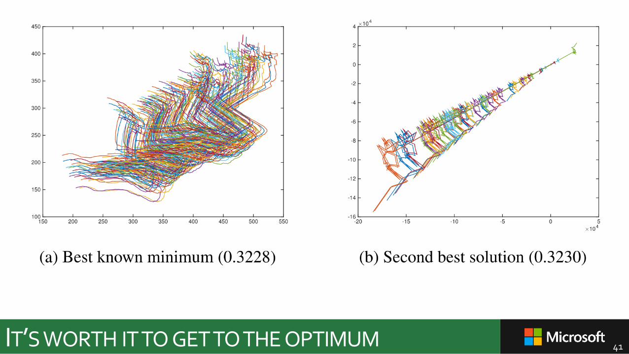
IT’S WORTH ITTO GETTOTHE OPTIMUM 41

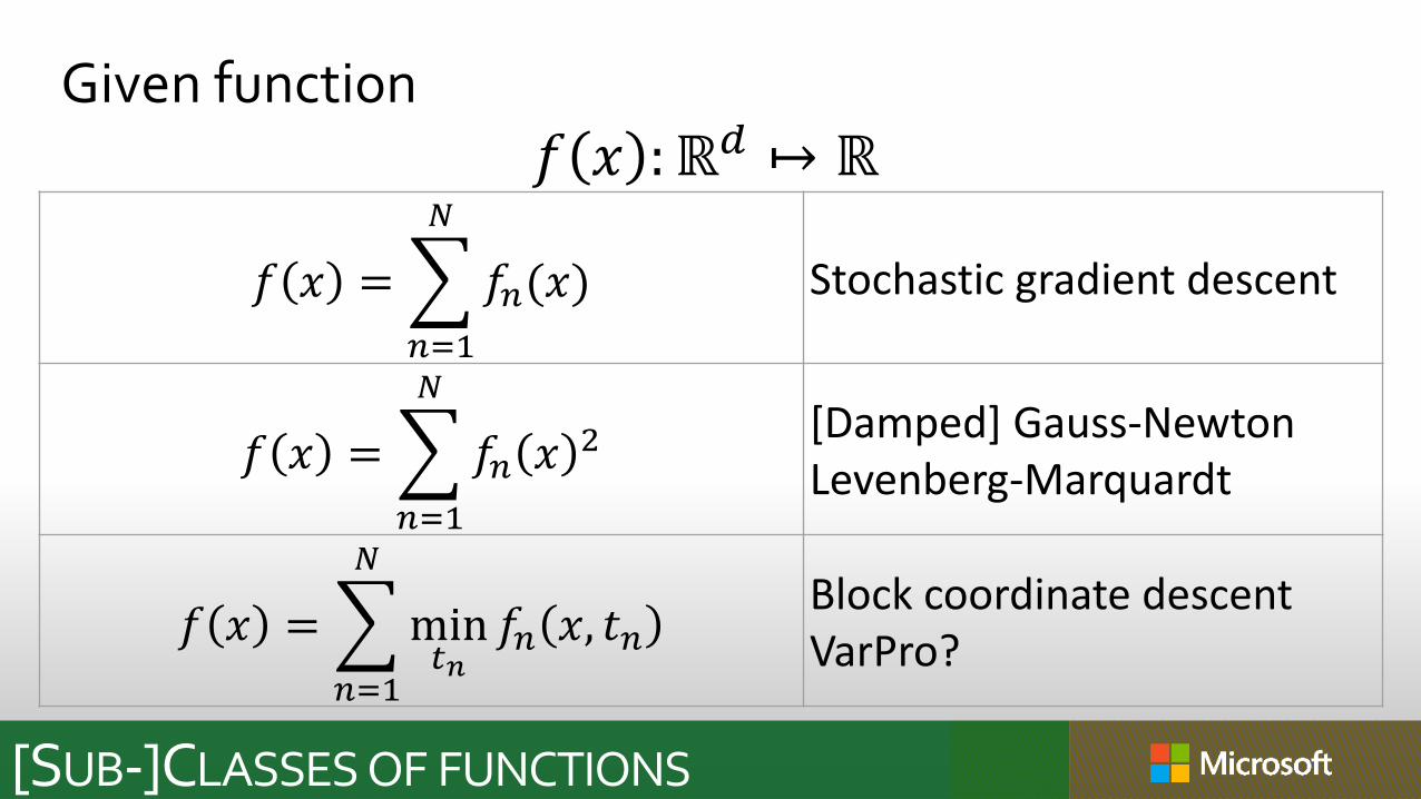
[SUB-]CLASSES OF FUNCTIONS

Given function𝑓 𝑥 :ℝ𝑑 ↦ ℝ

𝑓 𝑥 =

𝑛=1

𝑁

𝑓𝑛(𝑥) Stochastic gradient descent

𝑓 𝑥 =

𝑛=1

𝑁

𝑓𝑛 𝑥 2 [Damped] Gauss-NewtonLevenberg-Marquardt

𝑓 𝑥 =

𝑛=1

𝑁

min𝑡𝑛

𝑓𝑛 𝑥, 𝑡𝑛Block coordinate descentVarPro?

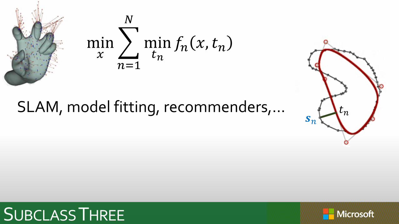
SUBCLASSTHREE

min𝑥

𝑛=1

𝑁

min𝑡𝑛

𝑓𝑛 𝑥, 𝑡𝑛

SLAM, model fitting, recommenders,...𝒔𝑛

𝑡𝑛

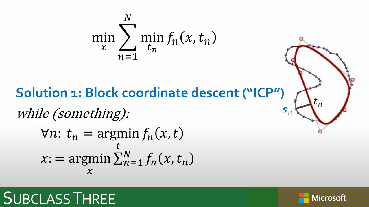
SUBCLASSTHREE

min𝑥

𝑛=1

𝑁

min𝑡𝑛

𝑓𝑛 𝑥, 𝑡𝑛

Solution 1: Block coordinate descent (“ICP”)

while (something):

∀𝑛: 𝑡𝑛 = argmin𝑡

𝑓𝑛 𝑥, 𝑡

𝑥: = argmin𝑥

σ𝑛=1𝑁 𝑓𝑛 𝑥, 𝑡𝑛

𝒔𝑛𝑡𝑛

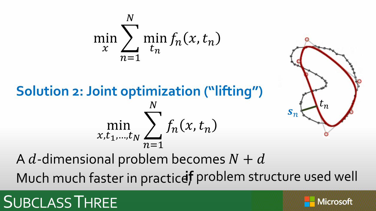
SUBCLASSTHREE

min𝑥

𝑛=1

𝑁

min𝑡𝑛

𝑓𝑛 𝑥, 𝑡𝑛

Solution 2: Joint optimization (“lifting”)

min𝑥,𝑡1,…,𝑡𝑁

𝑛=1

𝑁

𝑓𝑛 𝑥, 𝑡𝑛

A 𝑑-dimensional problem becomes 𝑁 + 𝑑

Much much faster in practice,

𝒔𝑛

if problem structure used well

𝑡𝑛

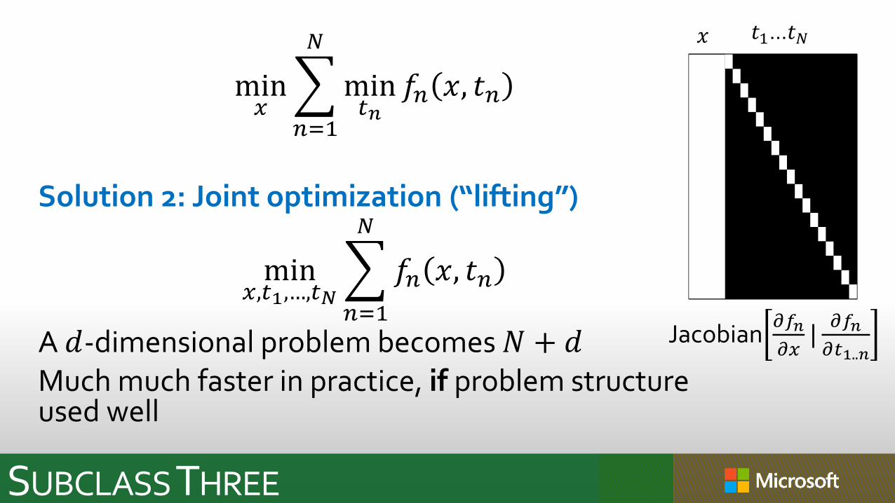
SUBCLASSTHREE

min𝑥

𝑛=1

𝑁

min𝑡𝑛

𝑓𝑛 𝑥, 𝑡𝑛

Solution 2: Joint optimization (“lifting”)

min𝑥,𝑡1,…,𝑡𝑁

𝑛=1

𝑁

𝑓𝑛 𝑥, 𝑡𝑛

A 𝑑-dimensional problem becomes 𝑁 + 𝑑Much much faster in practice, if problem structure used well

𝑥 𝑡1…𝑡𝑁

Jacobian𝜕𝑓𝑛

𝜕𝑥|𝜕𝑓𝑛

𝜕𝑡1..𝑛

AN EXEMPLARY PROBLEM

47

“Based on a true story”, not necessarily historically accurate

Note well: this problem is a good proxy for much more realistic problems:

1. Stereo camera calibration

2. Multiple-camera bundle adjustment

3. Surface fitting, e.g. subdivision surfaces to range data, realtime hand tracking

4. Matrix completion

5. Image denoising.

[From Neil Lawrence]

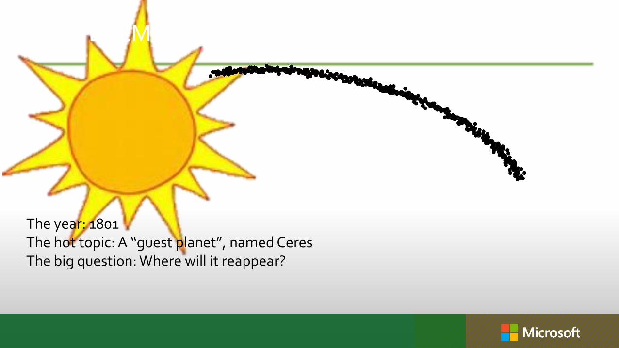
AN EXEMPLARY PROBLEM

The year: 1801The hot topic: A “guest planet”, named CeresThe big question: Where will it reappear?

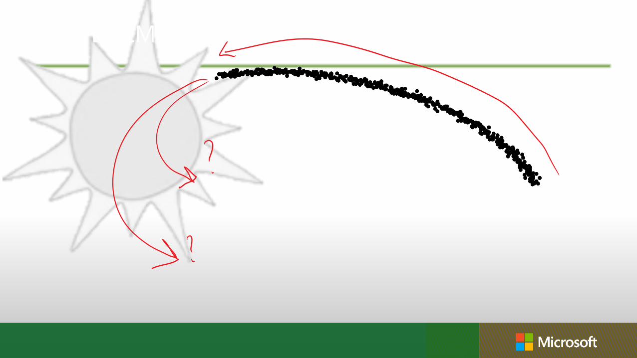
AN EXEMPLARY PROBLEM

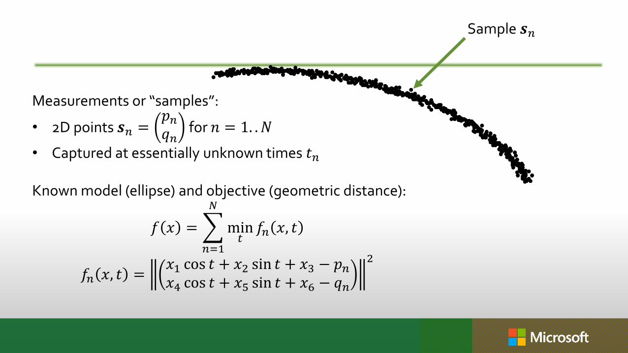
AN EXEMPLARY PROBLEM

Measurements or “samples”:

• 2D points 𝒔𝑛 =𝑝𝑛𝑞𝑛

for 𝑛 = 1. . 𝑁

• Captured at essentially unknown times 𝑡𝑛

Known model (ellipse) and objective (geometric distance):

𝑓 𝑥 =

𝑛=1

𝑁

min𝑡

𝑓𝑛 𝑥, 𝑡

𝑓𝑛 𝑥, 𝑡 =𝑥1 cos 𝑡 + 𝑥2 sin 𝑡 + 𝑥3 − 𝑝𝑛𝑥4 cos 𝑡 + 𝑥5 sin 𝑡 + 𝑥6 − 𝑞𝑛

2

Sample 𝒔𝑛

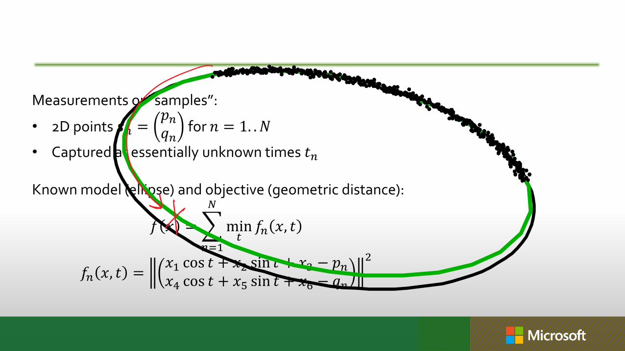
AN EXEMPLARY PROBLEM

Measurements or “samples”:

• 2D points 𝒔𝑛 =𝑝𝑛𝑞𝑛

for 𝑛 = 1. . 𝑁

• Captured at essentially unknown times 𝑡𝑛

Known model (ellipse) and objective (geometric distance):

𝑓 𝑥 =

𝑛=1

𝑁

min𝑡

𝑓𝑛 𝑥, 𝑡

𝑓𝑛 𝑥, 𝑡 =𝑥1 cos 𝑡 + 𝑥2 sin 𝑡 + 𝑥3 − 𝑝𝑛𝑥4 cos 𝑡 + 𝑥5 sin 𝑡 + 𝑥6 − 𝑞𝑛

2

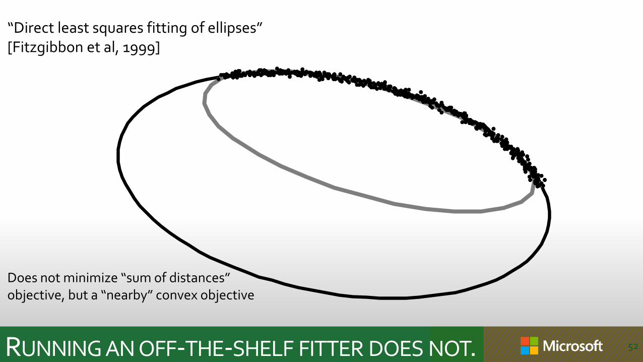
RUNNING AN OFF-THE-SHELF FITTER DOES NOT. 52

“Direct least squares fitting of ellipses”[Fitzgibbon et al, 1999]

Does not minimize “sum of distances” objective, but a “nearby” convex objective

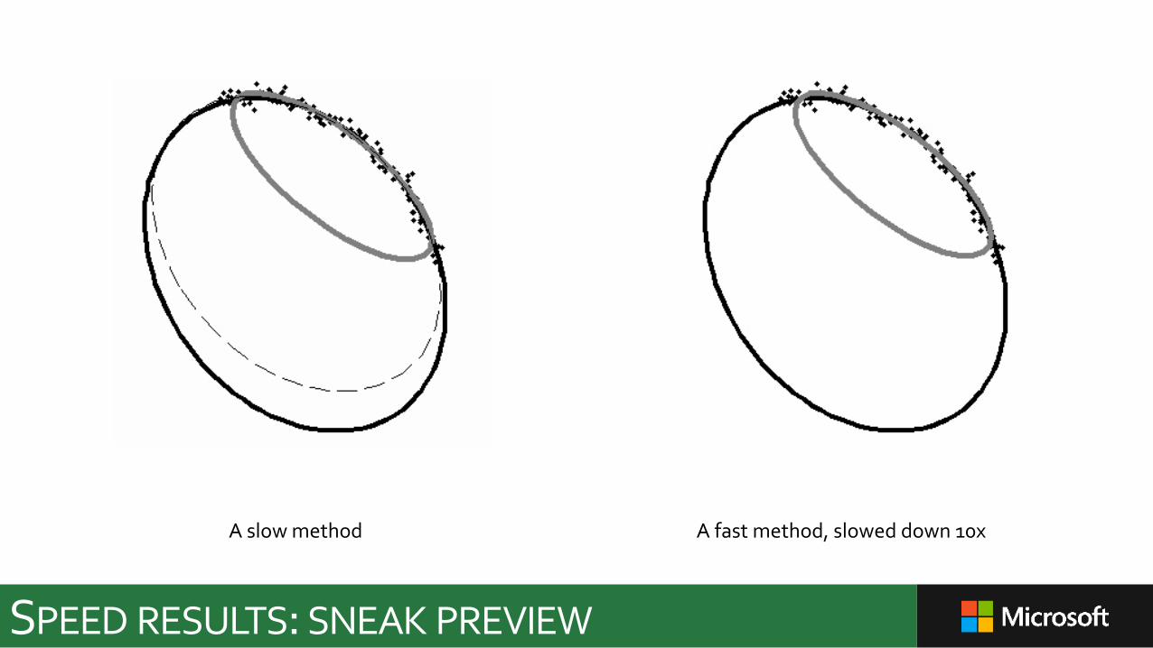
SPEED RESULTS: SNEAK PREVIEW

A slow method A fast method, slowed down 10x

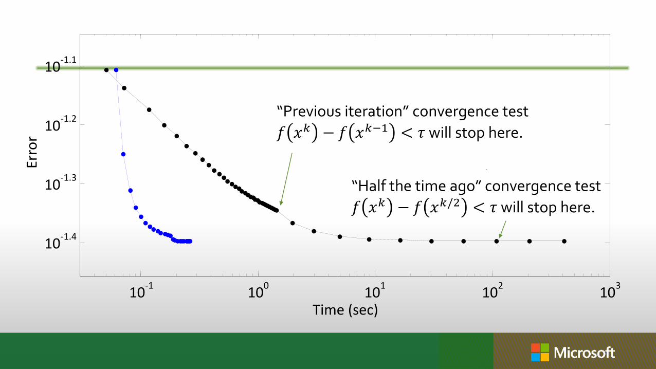
CONVERGENCE CURVES

10-1

100

101

102

103

10-1.4

10-1.3

10-1.2

10-1.1

Time (sec)

Erro

r

“Previous iteration” convergence test

𝑓 𝑥𝑘 − 𝑓 𝑥𝑘−1 < 𝜏 will stop here.

“Half the time ago” convergence test

𝑓 𝑥𝑘 − 𝑓 𝑥𝑘/2 < 𝜏 will stop here.

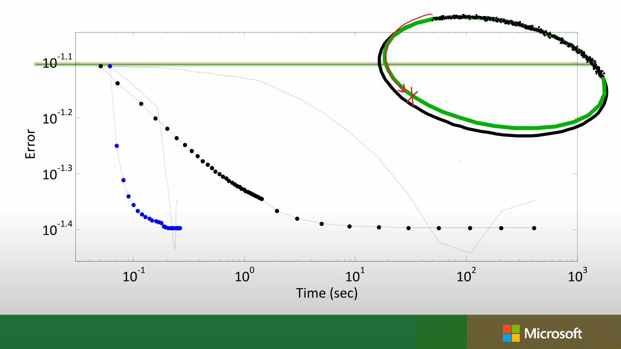
AH, BUT WHAT ABOUT TEST ERROR?

10-1

100

101

102

103

10-1.4

10-1.3

10-1.2

10-1.1

Time (sec)

Erro

r

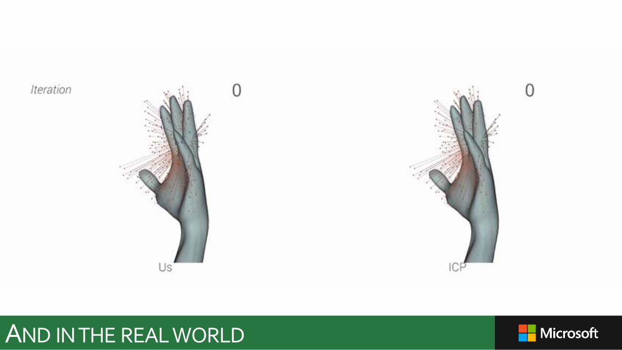
AND INTHE REAL WORLD

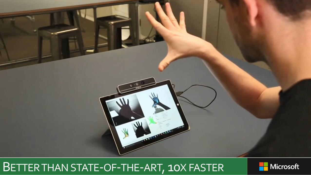
BETTER THAN STATE-OF-THE-ART, 10X FASTER

Bonus material

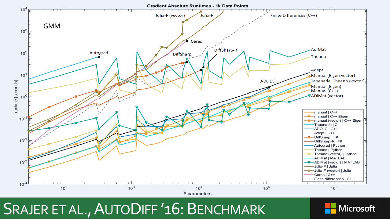
SRAJER ET AL., AUTODIFF ’16: BENCHMARK

GMM

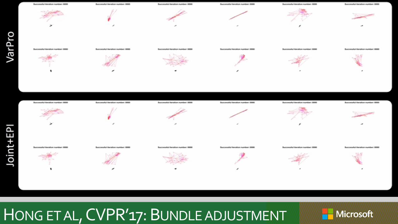
HONG ET AL, CVPR’17: BUNDLE ADJUSTMENT

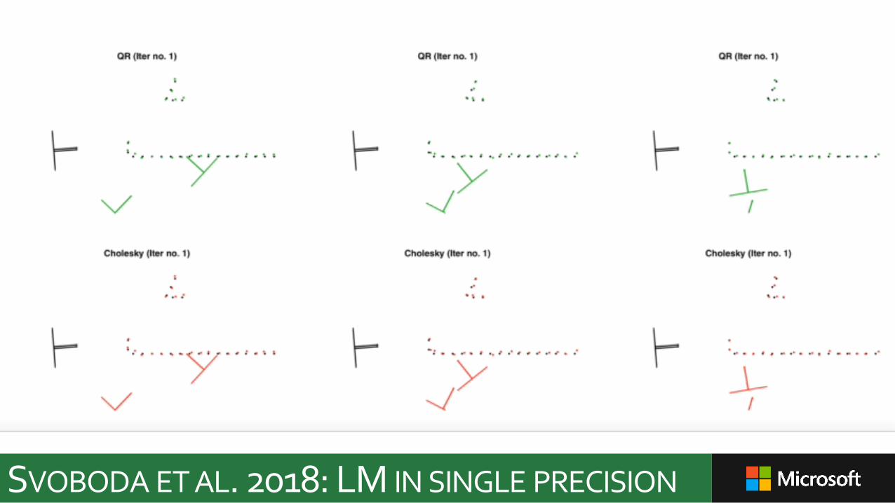
SVOBODA ET AL. 2018: LM IN SINGLE PRECISION

CONCLUSION

▪ Use discriminative machine learning (e.g. DNNs) to get near an optimum (e.g. down to 10 pixels)

▪ Use model fitting to get quality solutions (e.g. down to 0.1 pixels).

CONCLUSION

▪ “Non convex optimization is slow”

▪ “There’s no point in getting doing better than 1% off the optimum”

▪ “There’s no point in optimizing my code”

▪ “Bundle adjustment needs a good initialization”

Clichés

I want you

to stop

using