Embed Size (px)
DESCRIPTION
CHAPTER 3. Higher-Order Differential Equations. (3.1~3.6). Chapter Contents. 3.1 Theory of Linear Equations 3.2 Reduction of Order 3.3 Homogeneous Linear Equations with Constants Coefficients 3.4 Undetermined Coefficients 3.5 Variation of Parameters 3.6 Cauchy-Euler Equations. - PowerPoint PPT Presentation
Citation preview

Copyright © Jones and Bartlett;滄海書局 1
Higher-Order Differential Equations
CHAPTER 3
(3.1~3.6)
Copyright © Jones and Bartlett;滄海書局 Ch3_2
Chapter Contents
3.1 Theory of Linear Equations3.2 Reduction of Order3.3 Homogeneous Linear Equations with Constants C
oefficients3.4 Undetermined Coefficients3.5 Variation of Parameters3.6 Cauchy-Euler Equations
Copyright © Jones and Bartlett;滄海書局 Ch3_3
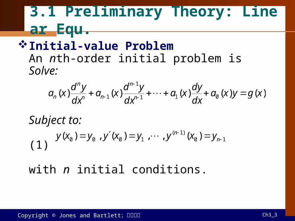
3.1 Preliminary Theory: Linear Equ.
Initial-value Problem An nth-order initial problem isSolve:
Subject to:
(1)
with n initial conditions.
)()()()()( 011
1
1 xgyxadxdy
xadx
ydxa
dxyd
xa n
n
nn
n
n
10)1(
1000 )(,,)(,)( n
n yxyyxyyxy

Copyright © Jones and Bartlett;滄海書局 Ch3_4
Let an(x), an-1(x), …, a0(x), and g(x) be continuous on I,
an(x) 0 for all x on I. If x = x0 is any point in this interval, then a solution y(x) of (1) exists on the interval and is unique.
Theorem 3.1.1 Existence of a Unique Solution

Copyright © Jones and Bartlett;滄海書局 Ch3_5
The IVP
possesses the trivial solution y = 0. Since this DE with constant coefficients, from Theorem 3.1.1, hence y = 0 is the only one solution on any interval containing x = 1.
Example 1 Unique Solution of an IVP
0)1(,0)1(,0)1(,0753 yyyyyyy

Copyright © Jones and Bartlett;滄海書局 Ch3_6
Example 2 Unique Solution of an VP
Please verify y = 3e2x + e–2x – 3x, is a solution of
This DE is linear and the coefficients and g(x) are all continuous, and a2(x) 0 on any I containing x = 0. This DE has an unique solution on I.
1)0(',4)0(,124" yyxyy
Copyright © Jones and Bartlett;滄海書局 Ch3_7
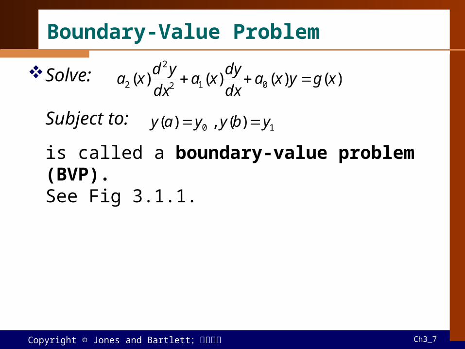
Boundary-Value Problem
Solve:
Subject to:
is called a boundary-value problem (BVP).See Fig 3.1.1.
)()()()( 012
2
2 xgyxadxdy
xadx
ydxa
10 )(,)( ybyyay

Copyright © Jones and Bartlett;滄海書局 Ch3_8
Fig 3.1.1 Colored curves are solution of a BVP

Copyright © Jones and Bartlett;滄海書局 Ch3_9
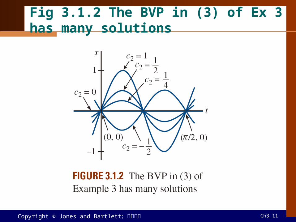
In example 4 of Sec 1.1, we see the solution of isx = c1 cos 4t + c2 sin 4t (2)
(a) Suppose x(0) = 0, then c1 = 0, x(t) = c2 sin 4tFurthermore, x(/2) = 0, we obtain 0 = 0, hence
(3)has infinite many solutions. See Fig 3.1.2.
(b) If(4)
we have c1 = 0, c2 = 0, x = 0 is the only solution.
Example 3 A BVP Can Have Money, Ine, or Not Solutions
016" xx
02
,0)0(,016
xxxx
08
,0)0(,016
xxxx

Copyright © Jones and Bartlett;滄海書局 Ch3_10
Example 3 (2)
(c) If
(5)we have c1 = 0, and 1 = 0 (contradiction).Hence (5) has no solutions.
12
,0)0(,016
xxxx
Copyright © Jones and Bartlett;滄海書局 Ch3_11
Fig 3.1.2 The BVP in (3) of Ex 3 has many solutions

Copyright © Jones and Bartlett;滄海書局 Ch3_12
Homogeneous Equations
The following DE
(6)
is said to be homogeneous;
(7)
with g(x) not identically zero, is nonhomogeneous.
0)()()()( 011
1
1
yxadxdy
xadx
ydxa
dxyd
xa n
n
nn
n
n
)()()()()( 011
1
1 xgyxadxdy
xadx
ydxa
dxyd
xa n
n
nn
n
n

Copyright © Jones and Bartlett;滄海書局 Ch3_13
Let dy/dx = Dy. This symbol D is called a differential operator. We define an nth-order differential operator as
(8)In addition, we have
(9)so the differential operator L is a linear operator.
Differential Equations We can simply write the DEs as
L(y) = 0 and L(y) = g(x)
Differential Operators
)()()()( 011
1 xaDxaDxaDxaL nn
nn
))(())(()}()({ xgLxfLxgxfL

Copyright © Jones and Bartlett;滄海書局 Ch3_14
Let y1, y2, …, yk be a solutions of the homogeneous
Nth-order differential equation (6) on an interval I.
Then the linear combinationy = c1y1(x) + c2y2(x) + …+ ckyk(x)
where the ci, i = 1, 2, …, k are arbitrary constants, is
also a solution on the interval.
Theorem 3.1.2 Superposition Principles – Homogeneous Equations
Copyright © Jones and Bartlett;滄海書局 Ch3_15
(a) y = cy1 is also a solution if y1 is a solution.
(b) A homogeneous linear DE always possesses the trivial solution y = 0.
Corollaries to Theorem 3.1.2

Copyright © Jones and Bartlett;滄海書局 Ch3_16
The function y1 = x2, y2 = x2 ln x are both solutions of
Then y = x2 + x2 ln x is also a solution on (0, ).
Example 4 Superposition – Homogeneous DE
A set of f1(x), f2(x), …, fn(x) is linearly dependent on
an interval I, if there exists constants c1, c2, …, cn,
not all zero, such that c1f1(x) + c2f2(x) + … + cn fn(x) = 0If not linearly dependent, it is linearly independent.
Definition 3.1.1 Linear Dependence / Independence
0423 yyxyx
Copyright © Jones and Bartlett;滄海書局 Ch3_17
In other words, if the set is linearly independent, when c1f1(x) + c2f2(x) + … + cn fn(x) = 0then c1 = c2 = … = cn = 0
Referring to Fig 3.1.3, neither function is a constant multiple of the other, then these two functions are linearly independent.
If two functions are linearly dependent, then one is simply a constant multiple of the other.
Two functions are linearly independent when neither is a constant multiple of the other.

Copyright © Jones and Bartlett;滄海書局 Ch3_18
Fig 3.1.3 The set consisting of f1 and f2 is linear independent on (-, )

Copyright © Jones and Bartlett;滄海書局 Ch3_19
The functions f1 = cos2 x, f2 = sin2 x, f3 = sec2 x, f4 = tan2 x are linearly dependent on the interval (-/2, /2) since
c1 cos2 x +c2 sin2 x +c3 sec2 x +c4 tan2 x = 0
when c1 = c2 = 1, c3 = -1, c4 = 1.
Example 5 Linear Dependent Functions

Copyright © Jones and Bartlett;滄海書局 Ch3_20
Example 6 Linearly Dependent Functions
The functions are linearly dependent on the interval (0, ), since
f2 = 1 f1 + 5 f3 + 0 f4
,1)( ,5)( ,5)( 321 xxfxxxfxxf2
4 )( xxf

Copyright © Jones and Bartlett;滄海書局 Ch3_21
Suppose each of the functions f1(x), f2(x), …, fn(x)
possesses at least n – 1 derivatives. The determinant
is called the Wronskian of the functions.
Definition 3.1.2 Wronskian
)1()1()1(
21
21
1
21
), ,...(
nn
nn
n
n
n
fff
fff
fff
ffW

Copyright © Jones and Bartlett;滄海書局 Ch3_22
Let y1(x), y2(x), …, yn(x) be n solutions of the nth-order
homogeneous DE (6) on an interval I. This set of
solutions is linearly independent on I if and on if
W(y1, y2, …, yn) 0 for every x in the interval.
Theorem 3.1.3 Criterion for Linear Independence Solutions
Copyright © Jones and Bartlett;滄海書局 Ch3_23
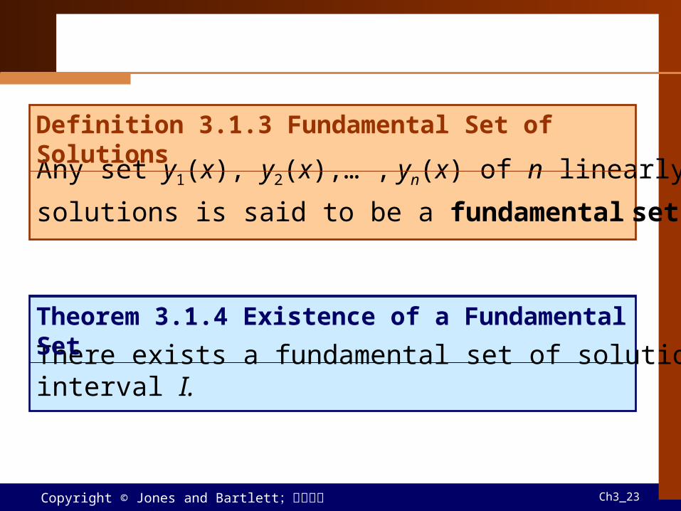
Any set y1(x), y2(x),… , yn(x) of n linearly independent
solutions is said to be a fundamental set of solutions.
Definition 3.1.3 Fundamental Set of Solutions
There exists a fundamental set of solutions for (6) on an interval I.
Theorem 3.1.4 Existence of a Fundamental Set

Copyright © Jones and Bartlett;滄海書局 Ch3_24
Let y1(x), y2(x), …, yn(x) be a fundamental set of
solutions of homogeneous DE (6) on an interval I. Then
the general solution is y = c1y1(x) + c2y2(x) + … + cnyn(x)
where ci, i = 1, 2, …, n are arbitrary constants.
Theorem 3.1.5 General Solution – Homogeneous Equations

Copyright © Jones and Bartlett;滄海書局 Ch3_25
The functions y1 = e3x, y2 = e-3x are solutions of y” – 9y = 0 on (-, )Now
for every x. So y = c1e3x + c2e-3x is the general solution.
Example 7 General Solution of a Homogeneous DE
0633
),(33
3333
xx
xxxx
ee
eeeeW

Copyright © Jones and Bartlett;滄海書局 Ch3_26
Example 8 A Solution Obtained from a General Solution
The functions y = 4 sinh 3x - 5e3x is a solution of example 7 (Verify it). Observer
y = 4 sinh 3x – 5e-3x
xxx
xxx eee
eeey 333
333 52
4522
Copyright © Jones and Bartlett;滄海書局 Ch3_27
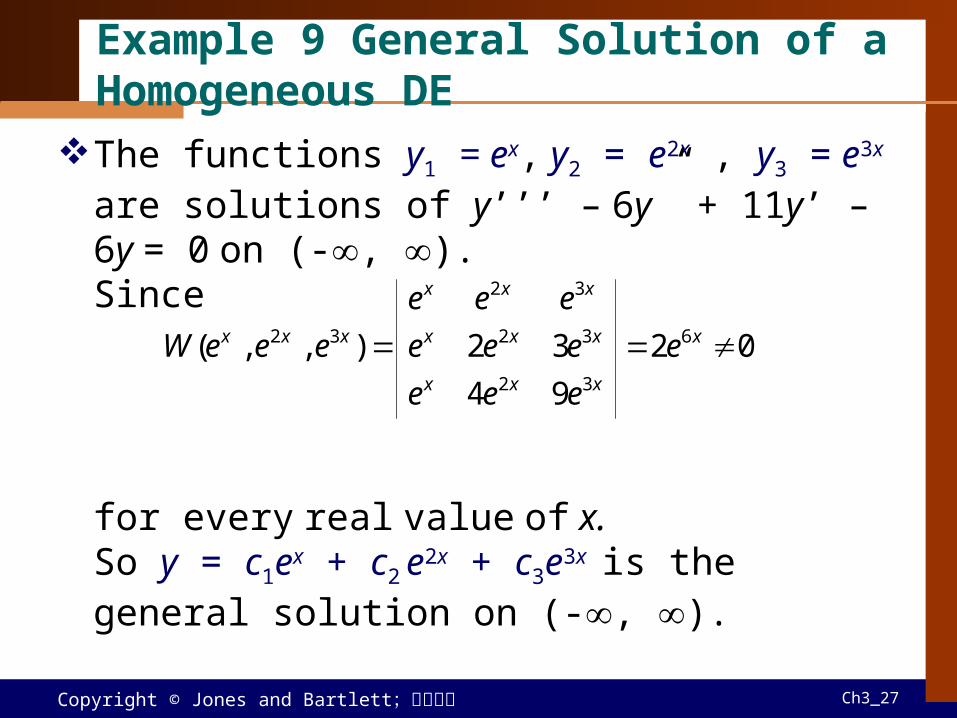
The functions y1 = ex, y2 = e2x , y3 = e3x are solutions of y’’’ – 6y” + 11y’ – 6y = 0 on (-, ). Since
for every real value of x. So y = c1ex + c2 e2x + c3e3x is the general solution on (-, ).
Example 9 General Solution of a Homogeneous DE
02
94
32),,( 6
32
32
32
32 x
xxx
xxx
xxx
xxx e
eee
eee
eee
eeeW
Copyright © Jones and Bartlett;滄海書局 Ch3_28
Nonhomogeneous Equations
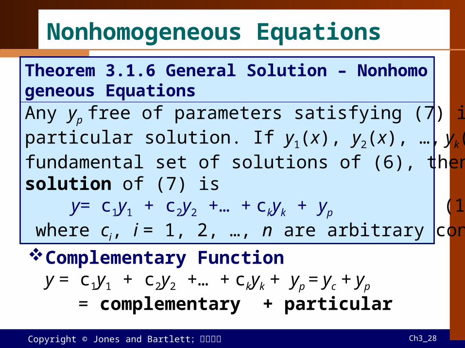
Complementary Functiony = c1y1 + c2y2 +… + ckyk + yp = yc + yp
= complementary + particular
Any yp free of parameters satisfying (7) is called a particular solution. If y1(x), y2(x), …, yk(x) be a fundamental set of solutions of (6), then the general solution of (7) is
y= c1y1 + c2y2 +… + ckyk + yp (10) where ci, i = 1, 2, …, n are arbitrary constants.
Theorem 3.1.6 General Solution – Nonhomogeneous Equations

Copyright © Jones and Bartlett;滄海書局 Ch3_29
The function yp = -(11/12) – ½ x is a particular solution of
(11)From previous discussions, the general solution of (11) is
Example 10 General Solution of a Nonhomogeneous DE
xyyyy 36116
xecececyyy xxxpc 2
112113
32
21

Copyright © Jones and Bartlett;滄海書局 Ch3_30
Given(12)
where i = 1, 2, …, k. If ypi denotes a particular solution corresponding to the
DE (12) with gi(x), then(13)
is a particular solution of (14)
Theorem 3.1.7 Superposition Principles – Nonhomogeneous Equations
Any Superposition Principles
)()()()()( 01)1(
1)( xgyxayxayxayxa i
nn
nn
)()()(21
xyxyxyykpppp
)()()(
)()()()(
21
01)1(
1)(
xgxgxg
yxayxayxayxa
k
nn
nn

Copyright © Jones and Bartlett;滄海書局 Ch3_31
We find is a particular solution of
is a particular solution of
is a particular solution of
From Theorem 3.1.7, is a solution of
Example 11 Superposition – Nonmogeneous DE
824164'3" 2 xxyyy
xeyyy 224'3"
xx exeyyy 24'3"
321 ppp yyyy
)()(
2
)(
2
321
228241643xg
xx
xg
x
xg
exeexxyyy
241
xy p
xp ey 2
2

Copyright © Jones and Bartlett;滄海書局 Ch3_32
If ypi is a particular solution of (12), then
is also a particular solution of (12) when the right-hand member is
Note
,21 21 kpkppp ycycycy
)()()( 2211 xgcxgcxgc kk

Copyright © Jones and Bartlett;滄海書局 Ch3_33
3.2 Reduction of Order
IntroductionWe know the general solution of
(1)is y = c1y1 + c2y1. Suppose y1(x) denotes a known solution of (1). We assume the other solution y2 has the form y2 = uy1.Our goal is to find a u(x) and this method is called reduction of order.
0)()()( 012 yxayxayxa
Copyright © Jones and Bartlett;滄海書局 Ch3_34
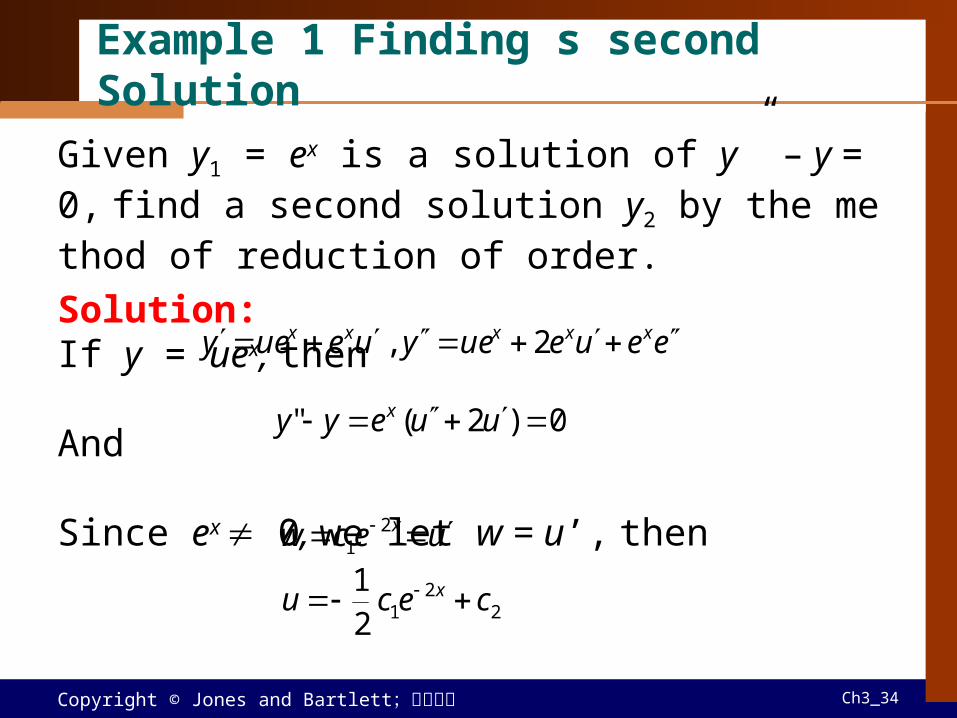
Given y1 = ex is a solution of y” – y = 0, find a second solution y2 by the method of reduction of order.
Solution:If y = uex, then
And
Since ex 0, we let w = u’, then
Example 1 Finding s second Solution
eeueueyueuey xxxxx 2,
0)2(" uueyy x
uecw x 21
22
121
cecu x

Copyright © Jones and Bartlett;滄海書局 Ch3_35
Thus (2)
Choosing c1 = 0, c2 = -2, we have y2 = e-x. Because W(ex, e-x) 0 for every x, they are independent on (-, ).
xxx ecec
exuy 21
2)(
Example 1 (2)
Copyright © Jones and Bartlett;滄海書局 Ch3_36
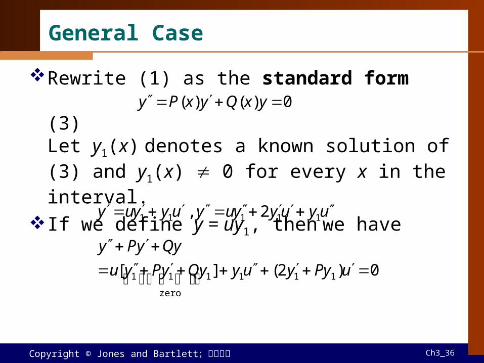
General Case
Rewrite (1) as the standard form (3)Let y1(x) denotes a known solution of (3) and y1(x) 0 for every x in the interval.
If we define y = uy1, then we have
0)()( yxQyxPy
uyuyyuyuyyuy 11111 2,
0)2(][ 111
zero
111
uPyyuyQyyPyu
QyyPy

Copyright © Jones and Bartlett;滄海書局 Ch3_37
This implies that
or(4)
where we let w = u’. Solving (4), we have
or
0)2( 111 uPyyuy
02)2( 111 wPyywy
021
1
Pdxdxyy
wdw
cPdxwy ||ln 21
Pdxecwy 121

Copyright © Jones and Bartlett;滄海書局 Ch3_38
then
Let c1 = 1, c2 = 0, we find
(5)
221
1 cdxy
ecu
Pdx
dxxy
exyy
dxxP
)()( 2
1
)(
12

Copyright © Jones and Bartlett;滄海書局 Ch3_39
The function y1= x2 is a solution of
Find the general solution on (0, ).
Solution:The standard form is
From (5)
The general solution is
Example 2 A second Solution by Formula (5)
04'3"2 yxyyx
043
2 yx
yx
y
xxdxx
exy
xdx
ln24
/32
2
xxcxcy ln22
21

Copyright © Jones and Bartlett;滄海書局 Ch3_40
3.3 Homogeneous Linear Equation with Constant Coefficients
Introduction (1)
where ai, i = 0, 1, …, n are constants, an 0.
Auxiliary EquationFor n = 2,
(2)Try y = emx, then
(3)
is called an auxiliary equation.
0012)1(
1)(
yayayayaya nn
nn
0 cyybya
0)( 2 cbmamemx
02 cbmam

Copyright © Jones and Bartlett;滄海書局 Ch3_41
From (3) the two roots are
(1) b2 – 4ac > 0: two distinct real numbers.(2) b2 – 4ac = 0: two equal real numbers.(3) b2 – 4ac < 0: two conjugate complex numbers.
aacbbm 2/)4( 21
aacbbm 2/)4( 22

Copyright © Jones and Bartlett;滄海書局 Ch3_42
Case 1: Distinct real rootsThe general solution is
(4)
Case 2: Repeated real roots and from (5) of Sec 3.2,
(5)
The general solution is
(6)
xmey 11
xmxmxm
xmxm xedxedx
ee
ey 11
1
1
1
2
2
2
xmxm xececy 1121
xmececy xm 2121

Copyright © Jones and Bartlett;滄海書局 Ch3_43
Case 3: Conjugate complex rootsWe write , a general solution is
From Euler’s formula: and (7) and
imim 21 ,
xixi eCeCy )(2
)(1
sincos iei xixe xi sincos xixe xi sincos
xee xixi cos2 xiee xixi sin2
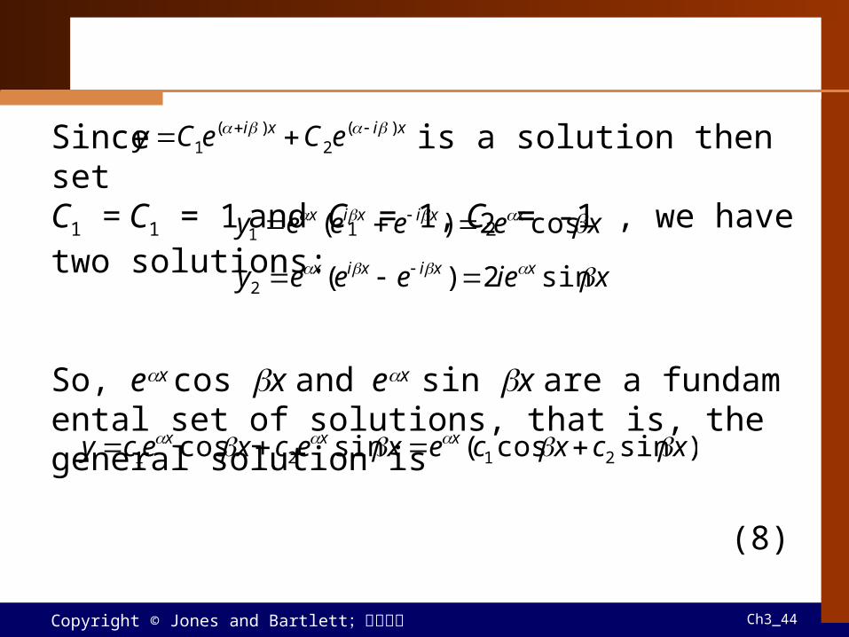
Copyright © Jones and Bartlett;滄海書局 Ch3_44
Since is a solution then setC1 = C1 = 1 and C1 = 1, C2 = -1 , we have two solutions:
So, ex cos x and ex sin x are a fundamental set of solutions, that is, the general solution is
(8)
xixi eCeCy )(2
)(1
xeeeey xxixix cos2)(1
xieeeey xxixix sin2)(2
)sincos(sincos 2121 xcxcexecxecy xxx

Copyright © Jones and Bartlett;滄海書局 Ch3_45
Solve the following DEs:
(a)
(b)
(c)
Example 1 Second-Order DEs
03'5"2 yyy
3,1/2,)3)(12(352 212 mmmmmm
xx ececy 32
2/1
025'10" yyy
5,)5(2510 2122 mmmmm
xx xececy 52
51
07'4" yyy
imimmm 32,32,074 212
)3sin3cos(,3,2 212 xcxcey x

Copyright © Jones and Bartlett;滄海書局 Ch3_46
Solve
Solution:
See Fig 3.3.1.
Example 2 An Initial-Value Problem
2)0(',1)0(,017'4"4 yyyyy
,01744 2 mm im 21/21
)2sin2cos( 212/ xcxcey x
,1)0( y ,11 c ,2)0(' and y 3/42 c

Copyright © Jones and Bartlett;滄海書局 Ch3_47
Fig 3.3.1 Graph of a solution of IVP in Ex 2

Copyright © Jones and Bartlett;滄海書局 Ch3_48
Two Equations worth Knowing
For the first equation:
(9)For the second equation:
(10)Let
Then(11)
,02 yky 0 ,02 kyky
kxckxcy sincos 21
kxkx ececy 21
kxckxcy sinhcosh 21
kxeey kxkx cosh)(1/21
kxeey kxkx sinh)(1/22

Copyright © Jones and Bartlett;滄海書局 Ch3_49
Higher-Order Equations
Given
(12)
we have
(13)
as an auxiliary equation.If the roots of (13) are real and distinct, then the
general solution of (12) is
0012)1(
1)(
yayayayaya nn
nn
0012
21
1 amamamama n
nn
n

Copyright © Jones and Bartlett;滄海書局 Ch3_50
Example 3 Third-Order DE
Solve
Solution:
043 yyy
2223 )2)(1()44)(1(43 mmmmmmm
232 mmxxx xecececy 2
32
21
Copyright © Jones and Bartlett;滄海書局 Ch3_51
Solve
Solution:
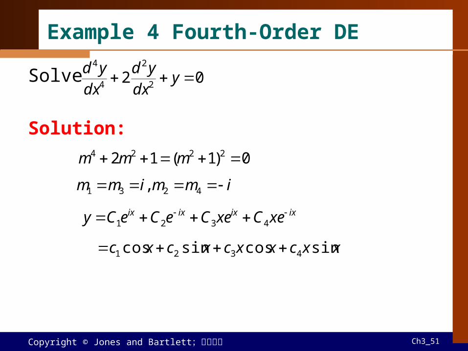
Example 4 Fourth-Order DE
02 2
2
4
4
ydx
yddx
yd
0)1(12 2224 mmm
immimm 4231 ,
ixixixix xeCxeCeCeCy 4321
xxcxxcxcxc sincossincos 4321

Copyright © Jones and Bartlett;滄海書局 Ch3_52
If m1 = + i is a complex root of multiplicity k, then m2 = − i is also a complex root of multiplicity k. The 2k linearly independent solutions:
Repeated complex roots
xexxexxxexe xkxxx cos,,cos,cos,cos 12
xexxexxxexe xkxxx sin,,sin,sin,sin 12

Copyright © Jones and Bartlett;滄海書局 Ch3_53
3.4 Undetermined Coefficients
IntroductionIf we want to solve
(1)
we have to find y = yc + yp. Thus we introduce the method of undetermined coefficients.
)(01)1(
1)( xgyayayaya n
nn
n

Copyright © Jones and Bartlett;滄海書局 Ch3_54
Solve (2)
Solution: We can get yc as described in Sec 3.3. Now, we want to find yp.
Since the right side of the DE is a polynomial, we set
After substitution, 2A + 8Ax + 4B – 2Ax2 – 2Bx – 2C = 2x2 – 3x + 6
Example 1 General Solution Using Undetermined Coefficients
6322'4 2 xxyyy
,2 CBxAxy p ,2, BAxyy pp Ay p 2

Copyright © Jones and Bartlett;滄海書局 Ch3_55
Example 1 (2)
Then6242,328,22 CBABAA
9,5/2,1 CBA
9252 xxy p
Copyright © Jones and Bartlett;滄海書局 Ch3_56
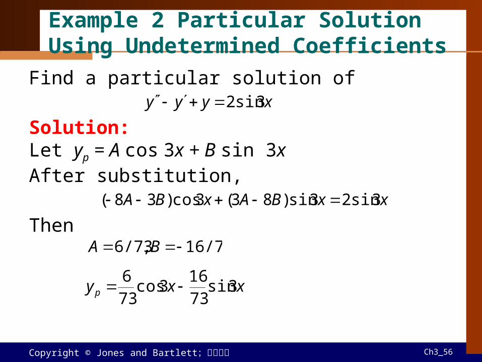
Find a particular solution of
Solution: Let yp = A cos 3x + B sin 3xAfter substitution,
Then
Example 2 Particular Solution Using Undetermined Coefficients
xyyy 3sin2
xxBAxBA 3sin23sin)83(3cos)38(
16/73,6/73 BA
xxy p 3sin7316
3cos736

Copyright © Jones and Bartlett;滄海書局 Ch3_57
Example 3 Forming yp by Superposition
Solve (3)
Solution: We can find
Let After substitution,
Then
xxexyyy 265432
xxc ececy 3
21
xxp EeCxeBAxy 22
xxx xexeECCxeBAAx 222 654)32(3323
4/3,2,23/9,4/3 ECBA
xxp exexy 22
34
2923
34
xxx exxececy 2321 3
42
923
34

Copyright © Jones and Bartlett;滄海書局 Ch3_58
Find yp of
Solution: First let yp = Ae2x
After substitution, 0 = 8e2x, (wrong guess)
Let yp = Axex
After substitution, -3Ae2x = 8e2x Then A = -8/3, yp = (−8/3)xe2x
Example 4 A Glitch in the Method
xeyyy 845

Copyright © Jones and Bartlett;滄海書局 Ch3_59
No function in the assumed yp is part of yc
Table 3.4.1 shows the trial particular solutions.
Case I
Copyright © Jones and Bartlett;滄海書局 Ch3_60
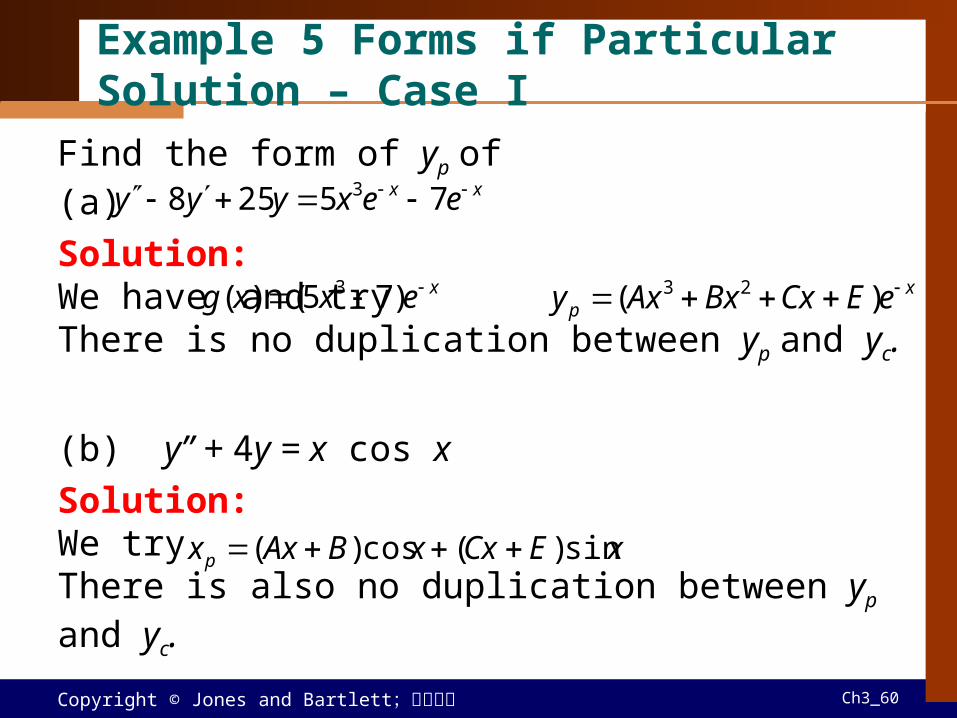
Example 5 Forms if Particular Solution – Case I
Find the form of yp of (a)
Solution: We have and tryThere is no duplication between yp and yc.
(b) y” + 4y = x cos x
Solution: We try There is also no duplication between yp and yc.
xx eexyyy 75258 3
xexxg )75()( 3 xp eECxBxAxy )( 23
xECxxBAxxp sin)(cos)(

Copyright © Jones and Bartlett;滄海書局 Ch3_61
Rule of Case I
If g(x) consists of a sum of m terms of the kind listed in the table, then (as in Ex 3) the assumption for a particular solution yp consists of the sum of the trial forms
The form of yp is a linear combination of all linearly independent functions that are generated by repeated differentiations of g(x).

Copyright © Jones and Bartlett;滄海書局 Ch3_62
Find the form of yp of
Solution: For 3x2:
For -5 sin 2x:
For 7xe6x:
No term in duplicates a term in yc
Example 6 Forming yp by Superposition – Case I
xxexxyyy 62 72sin53149
CBxAxy p 2
1
xFxEy p 2sin2cos2
xp eHGxy 6)(
3
321 pppp yyyy

Copyright © Jones and Bartlett;滄海書局 Ch3_63
Example 7 Particular Solution – Case II
Find a particular solution of
Solution:
The complementary function is yp = c1ex + c2xex.Assume yp = Aex will fail since it is apparent from yc that ex is a solution of the associated homogeneous equation
And we will not be able to find a particular solution of the form yp = Axex since the term xex is also duplicated in yc. We next try yp = Ax2ex, substituting into the given differential equation yields 2Axex = ex and so A = ½. The a particular solution is yp = ½x2ex.
xeyyy 2
.02 yyy
Copyright © Jones and Bartlett;滄海書局 Ch3_64
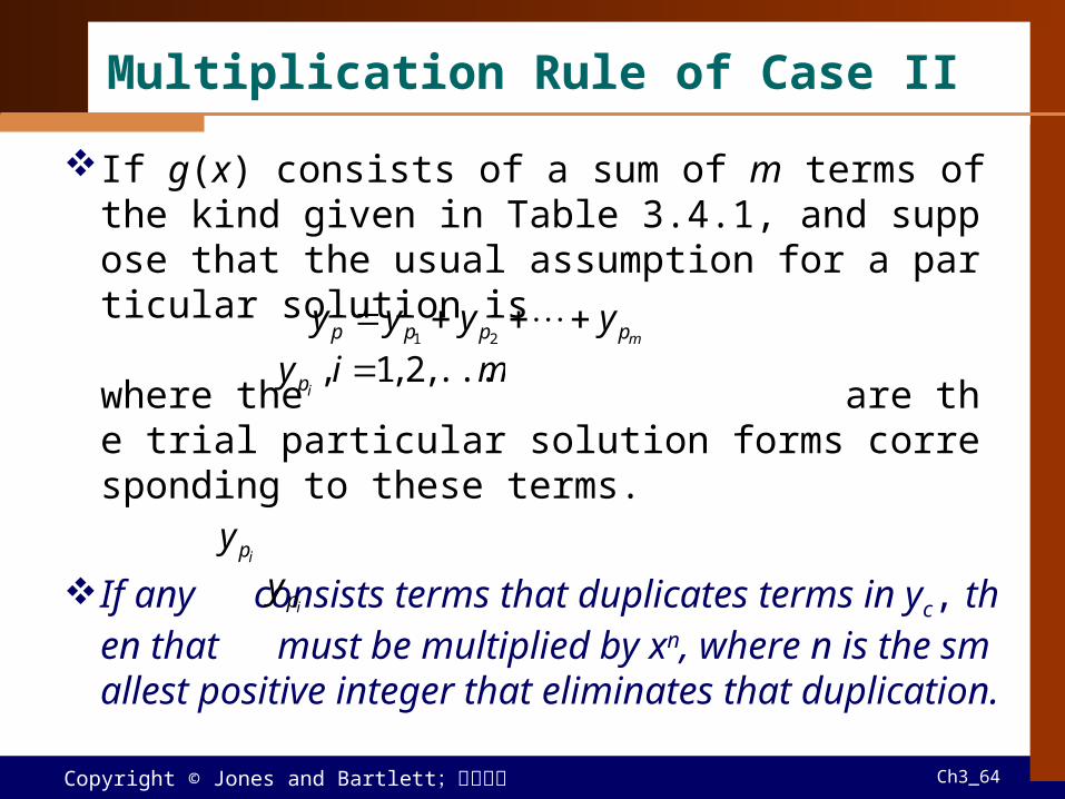
If g(x) consists of a sum of m terms of the kind given in Table 3.4.1, and suppose that the usual assumption for a particular solution is
where the are the trial particular solution forms corresponding to these terms.
If any consists terms that duplicates terms in yc, then that must be multiplied by xn, where n is the smallest positive integer that eliminates that duplication.
Multiplication Rule of Case II
mpppp yyyy 21
miyip ..., ,2 ,1 ,
ipy
ipy

Copyright © Jones and Bartlett;滄海書局 Ch3_65
Example 8 An Initial-Value Problem
Solve
Solution:
First trial: yp = Ax + B + C cos x + E sin x (5)However, duplication occurs. Then we try
yp = Ax + B + Cx cos x + Ex sin xAfter substitution and simplification,
A = 4, B = 0, C = -5, E = 0Then y = c1 cos x + c2 sin x + 4x – 5x cos xUsing y() = 0, y’() = 2, we have
y = 9 cos x + 7 sin x + 4x – 5x cos x
2)(',0)(,sin104" yyxxyy
xcxcyc sincos 21

Copyright © Jones and Bartlett;滄海書局 Ch3_66
Solve
Solution: yc = c1e3x + c2xe3x
After substitution and simplification,A = 2/3, B = 8/9, C = 2/3, E = -6
Then
Example 9 Using the multiplication Rule
xexyyy 32 12269'6"
21
32
ppy
x
y
p EeCBxAxy
xxx exxxxececy 32232
31 6
32
98
32

Copyright © Jones and Bartlett;滄海書局 Ch3_67
Solve
Solution: m3 + m2 = 0, m = 0, 0, -1yc = c1+ c2x + c3e-x yp = Aex cos x + Bex sin x
After substitution and simplification,A = -1/10, B = 1/5
Then
Example 10 Third-Order-DE CeasI
xeyy x cos"
xexeecxccyyy xxxpc sin
51
cos101
321
Copyright © Jones and Bartlett;滄海書局 Ch3_68
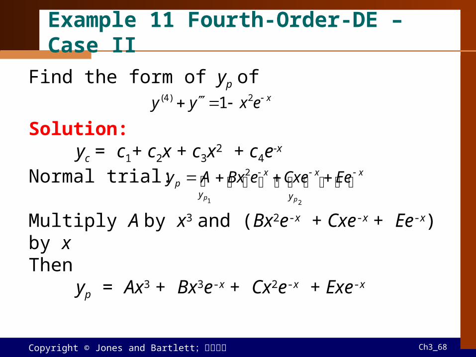
Find the form of yp of
Solution: yc = c1+ c2x + c3x2 + c4e-x
Normal trial:
Multiply A by x3 and (Bx2e-x + Cxe-x + Ee-x) by xThen
yp = Ax3 + Bx3e-x + Cx2e-x + Exe-x
Example 11 Fourth-Order-DE – Case II
xexyy 2)4( 1
21
2
pp y
xxx
yp EeCxeeBxAy

Copyright © Jones and Bartlett;滄海書局 Ch3_69
3.5 Variation of Parameters
Some Assumptions For the DE
(1)we put (1) in the form
(2)where P, Q, f are continuous on I.
)()()()( 012 xgyxayxayxa
)()()( xfyxQyxPy
Copyright © Jones and Bartlett;滄海書局 Ch3_70
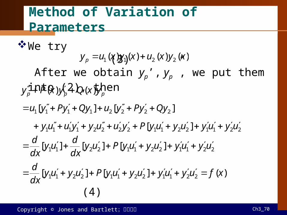
Method of Variation of Parameters
We try
(3) After we obtain yp’, yp”, we put them into (2), then
(4)
)()()()( 2211 xyxuxyxuy p
ppp yxQyxPy )()(
][][ 22221111 QyyPyuQyyPyu
2211221122221111 ][ uyuyuyuyPyuuyyuuy
221122112211 ][][][ uyuyuyuyPuydxd
uydxd
)(][][ 221122112211 xfuyuyuyuyPuyuydxd
Copyright © Jones and Bartlett;滄海書局 Ch3_71
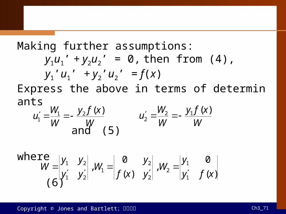
Making further assumptions: y1u1’ + y2u2’ = 0, then from (4),y1’u1’ + y2’u2’ = f(x)
Express the above in terms of determinants
and (5)
where
(6)
Wxfy
WW
u)(21
1 W
xfyWW
u)(12
2
)(
0,
)(
0,
1
12
2
21
21
21
xfy
yW
yxf
yW
yy
yyW

Copyright © Jones and Bartlett;滄海書局 Ch3_72
Solve
Solution: m2 – 4m + 4 = 0, m = 2, 2 y1 = e2x, y2 = xe2x,
Since f(x) = (x + 1)e2x, then
Example 1 General Solution Using Variation of Parameters
xexyyy 2)1(4'4"
022
),( 4
222
2222
x
xxx
xxxx e
exee
xeexeeW
x
xx
xx
xx
x
exexe
eWxex
xeex
xeW 4
22
2
24
22
2
1 )1()1(2
0,)1(
2)1(
0
Copyright © Jones and Bartlett;滄海書局 Ch3_73
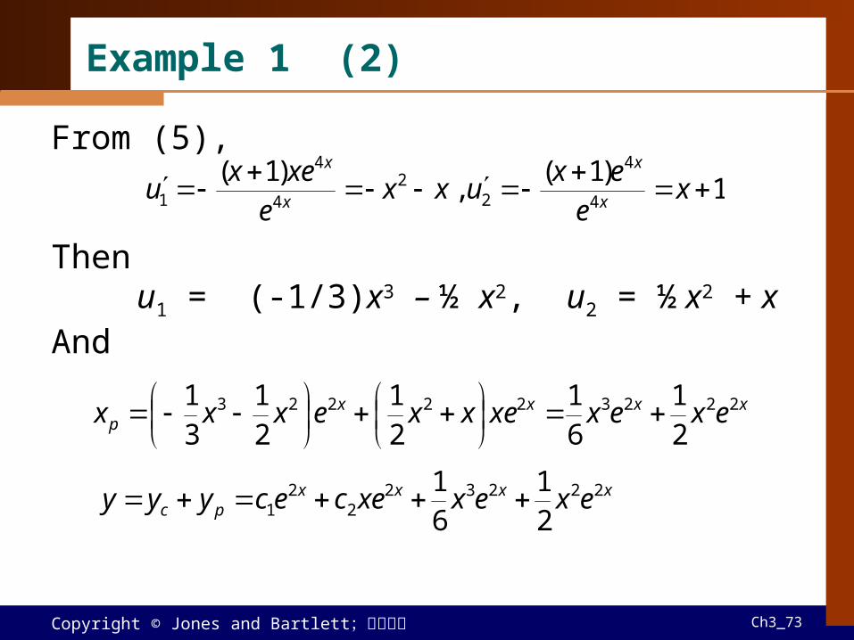
From (5),
Then
u1 = (-1/3)x3 – ½ x2, u2 = ½ x2 + xAnd
1)1(
,)1(
4
4
22
4
4
1 xe
exuxx
exex
u x
x
x
x
xxxxp exexxexxexxx 222322223
21
61
21
21
31
xxxxpc exexxececyyy 22232
22
1 21
61
Example 1 (2)

Copyright © Jones and Bartlett;滄海書局 Ch3_74
Solve
Solution: y” + 9y = (1/4) csc 3xm2 + 9 = 0, m = 3i, -3i y1 = cos 3x, y2 = sin 3x, f = (1/4) csc 3x
Since
Example 2 General Solution Suing Variation of Parameters
xyy 3csc364
33cos33sin3
3sin3cos)3sin,3(cos
xx
xxxxW
xx
xx
xW
xx
xW
3sin3cos
41
3csc4/13sin3
03cos
,41
3cos33csc4/1
3sin0
2
1

Copyright © Jones and Bartlett;滄海書局 Ch3_75
Then
And
(7)
1211
1 WW
u
xx
WW
u3sin3cos
1212
2
,12/11 xu |3sin|ln36/12 xu
|3sin|ln)3(sin361
3cos121
xxxxy p
|3sin|ln)3(sin361
3cos121
3sin3cos 21 xxxxxcxc
yyy pc
Example 2 (2)

Copyright © Jones and Bartlett;滄海書局 Ch3_76
Solve
Solution: m2 – 1 = 0, m = 1, -1 y1 = ex, y2 = e-x, f = 1/x, and W(ex, e-x) = -2
Then
The low and up bounds of the integral are x0 and x, respectively.
Example 3 General Solution Using Variation pf Paramenters
xyy
1
x
x
tx
dtt
eu
xeu
021
,2
)/1(11
x
x
tx
dtte
uxe
u02
1,
2)/1(
22

Copyright © Jones and Bartlett;滄海書局 Ch3_77
Example 3 (2)
x
x
x
x
tx
tx
p dtte
edtt
eey
0 021
21
x
x
x
x
tx
txxx
pc dtte
edtt
eeececyyy
0 021
21
21

Copyright © Jones and Bartlett;滄海書局 Ch3_78
For the DEs of the form
(8)
then yp = u1y1 + u2y2 + … + unyn, where yi , i = 1, 2, …, n, are the elements of yc. Thus we have
(9)
and uk’ = Wk/W, k = 1, 2, …, n.
Higher-Order Equations
)()()()( 01)1(
1)( xfyxPyxPyxPy n
nn
02211 nnuyuyuy
02211 nnuyuyuy
)()1(2
)1(21
)1(1 xfuyuyuy n
nn
nn

Copyright © Jones and Bartlett;滄海書局 Ch3_79
For the case n = 3,
(10)
,11 W
Wu ,2
2 WW
u WW
u 33
321
321
321
21
21
21
3
31
31
31
2
32
32
32
1
and
)(
0
0
,
)(
0
0
,
)(
0
0
yyy
yyy
yyy
W
xfyy
yy
yy
W
yxfy
yy
yy
W
yyxf
yy
yy
W
Copyright © Jones and Bartlett;滄海書局 Ch3_80
3.6 Cauchy-Eulaer Equation
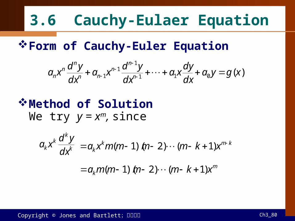
Form of Cauchy-Euler Equation
Method of SolutionWe try y = xm, since
)(011
11
1 xgyadxdy
xadx
ydxa
dxyd
xa n
nn
nn
nn
n
k
kk
k dxyd
xa kmkk xkmmmmxa )1()2)(1(
mk xkmmmma )1()2)(1(

Copyright © Jones and Bartlett;滄海書局 Ch3_81
An Auxiliary Equation
For n = 2, y = xm, thenam(m – 1) + bm + c = 0, oram2 + (b – a)m + c = 0
(1)
Case 1: Distinct Real Roots
(2)
2121
mm xcxcy
Copyright © Jones and Bartlett;滄海書局 Ch3_82
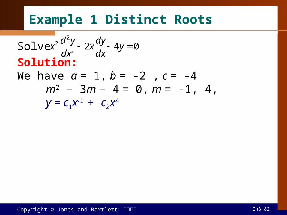
Solve
Solution:We have a = 1, b = -2 , c = -4
m2 – 3m – 4 = 0, m = -1, 4,y = c1x-1 + c2x4
Example 1 Distinct Roots
0422
22 y
dxdy
xdx
ydx

Copyright © Jones and Bartlett;滄海書局 Ch3_83
Using (5) of Sec 3.2, we have Then
(3)
Case 2: Repeated Real Roots
xxcxcy mm ln1121
xxy m ln12

Copyright © Jones and Bartlett;滄海書局 Ch3_84
Example 2 Repeated Roots
Solve
Solution:We have a = 4, b = 8, c = 1
4m2 + 4m + 1 = 0, m = -½ , -½
084 2
22 y
dxdy
xdx
ydx
xxcxcy ln2/12
2/11

Copyright © Jones and Bartlett;滄海書局 Ch3_85
Higher-Order: multiplicity
Case 3: Conjugate Complex Rootsm1 = + i, m2 = – i, y = C1x( + i) + C2x( - i)
Sincexi = (eln x)i = ei ln x = cos( ln x) + i sin( ln x)x-i = cos ( ln x) – i sin ( ln x)
Then y = c1x cos( ln x) + c2x sin( ln x) = x [c1 cos( ln x) + c2
sin( ln x)] (4)
Case 3: Conjugate Complex Roots
12 )(ln,,)(ln,ln, 1111 kmmmm xxxxxxx
Copyright © Jones and Bartlett;滄海書局 Ch3_86
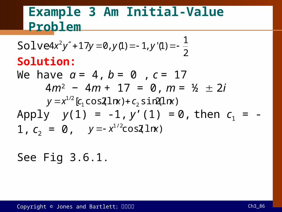
Solve
Solution:We have a = 4, b = 0 , c = 17
4m2 − 4m + 17 = 0, m = ½ 2i
Apply y(1) = -1, y’(1) = 0, then c1 = -1, c2 = 0,
See Fig 3.6.1.
Example 3 Am Initial-Value Problem
21
)1(',1)1(,0174 2 yyyyx
)]ln2sin()ln2cos([ 212/1 xcxcxy
)ln2cos(1/2 xxy

Copyright © Jones and Bartlett;滄海書局 Ch3_87
Fig 3.6.1 Graph of solution of IVP in Ex 3

Copyright © Jones and Bartlett;滄海書局 Ch3_88
Example 4 Third-Order Equation
Solve
Solution:Let y = xm,
Then we have xm(m + 2)(m2 + 4) = 0m = -2, m = 2i, m = -2iy = c1x-2 + c2 cos(2 ln x) + c3
sin(2 ln x)
0875 2
22
3
33 y
dxdy
xdx
ydx
dxyd
x
33
3
22
21
)2)(1(
,)1(,
m
mm
xmmmdx
yd
xmmdx
ydmx
dxdy
Copyright © Jones and Bartlett;滄海書局 Ch3_89
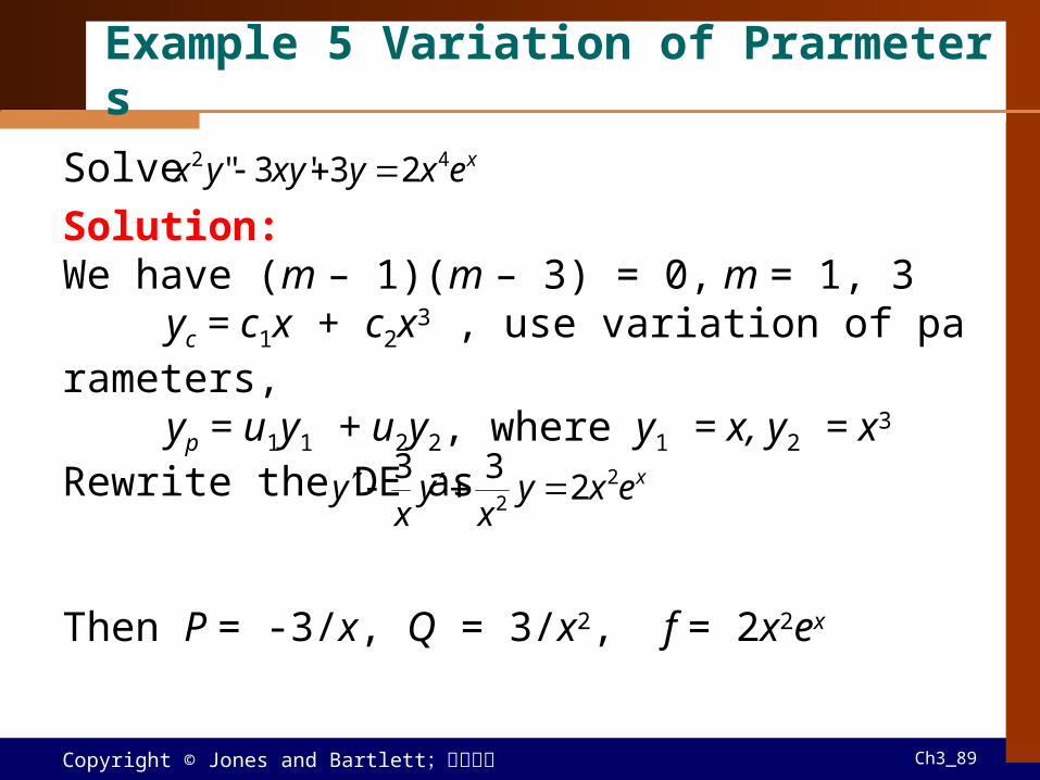
Solve
Solution:We have (m – 1)(m – 3) = 0, m = 1, 3 yc = c1x + c2x3 , use variation of parameters,
yp = u1y1 + u2y2, where y1 = x, y2 = x3 Rewrite the DE as
Then P = -3/x, Q = 3/x2, f = 2x2ex
Example 5 Variation of Prarmeters
xexyxyyx 42 23'3"
xexyx
yx
y 22 2
33

Copyright © Jones and Bartlett;滄海書局 Ch3_90
Thus
We find
xx
x
xex
ex
xWex
xex
xW
xx
xxW
322
5
22
3
1
3
2
3
221
0,2
32
0
,231
,2
2 23
5
1x
x
exxex
u xx
exex
u 3
5
2 22
,2221
xxx exeexu xeu 2
Example 5 (2)

Copyright © Jones and Bartlett;滄海書局 Ch3_91
Example 5 (3)
Then
xx
xxxxp
xeex
xexexeexyuyuy
22
)22(2
322211
xxpc xeexxcxcyyy 22 23
21
Copyright © Jones and Bartlett;滄海書局 92