Embed Size (px)
Citation preview
National EnergyTechnology Laboratory
Mehrdad Shahnam
Department of Energy
National Energy Technology Laboratory
High Performance Computing and Uncertainty Quantification
2015 WVU High Performance Computing Day, Waterfront Place Hotel, Morgantown, WV , April 16 2015
https://mfix.netl.doe.gov/
• Mehrdad Shahnam, DOE-NETL
• Aytekin Gel, ALPEMI Consulting LLC
• Arun Subramaniyan, GE Global Research Center
• Jordan Musser, DOE-NETL
• Jean Dietiker, WVURC
• Aniruddha Choudhary, Post Doctoral Fellow
Team Members
https://mfix.netl.doe.gov/
• Mission: Provide advanced high performance computing capabilities to accelerate progress in NETL programs to meet DOE’s Fossil Energy mission
• The NETL HPC consists of:
– NETL Supercomputer
– Modular Data Center (MDC) – The structure with high speed connectivity (in/out) that houses, powers and cools the system
– Visualization Centers – located at all NETL sites
High Performance Computing at NETL
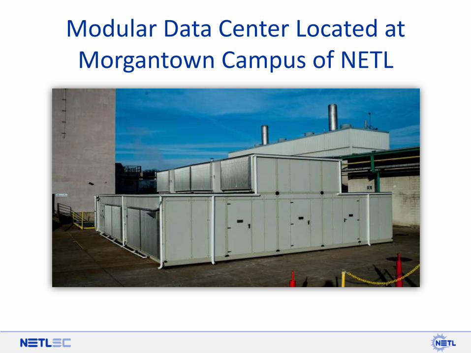
Modular Data Center Located at Morgantown Campus of NETL
https://mfix.netl.doe.gov/
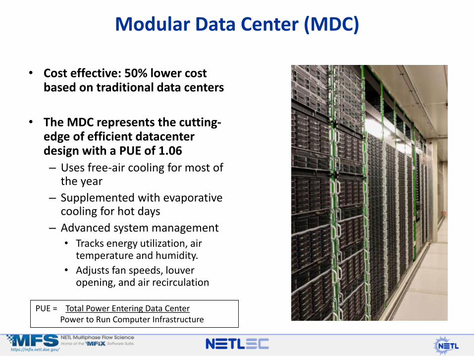
Modular Data Center (MDC)
• Cost effective: 50% lower cost based on traditional data centers
• The MDC represents the cutting-edge of efficient datacenter design with a PUE of 1.06
– Uses free-air cooling for most of the year
– Supplemented with evaporative cooling for hot days
– Advanced system management• Tracks energy utilization, air
temperature and humidity.
• Adjusts fan speeds, louver opening, and air recirculation
PUE = Total Power Entering Data CenterPower to Run Computer Infrastructure
https://mfix.netl.doe.gov/
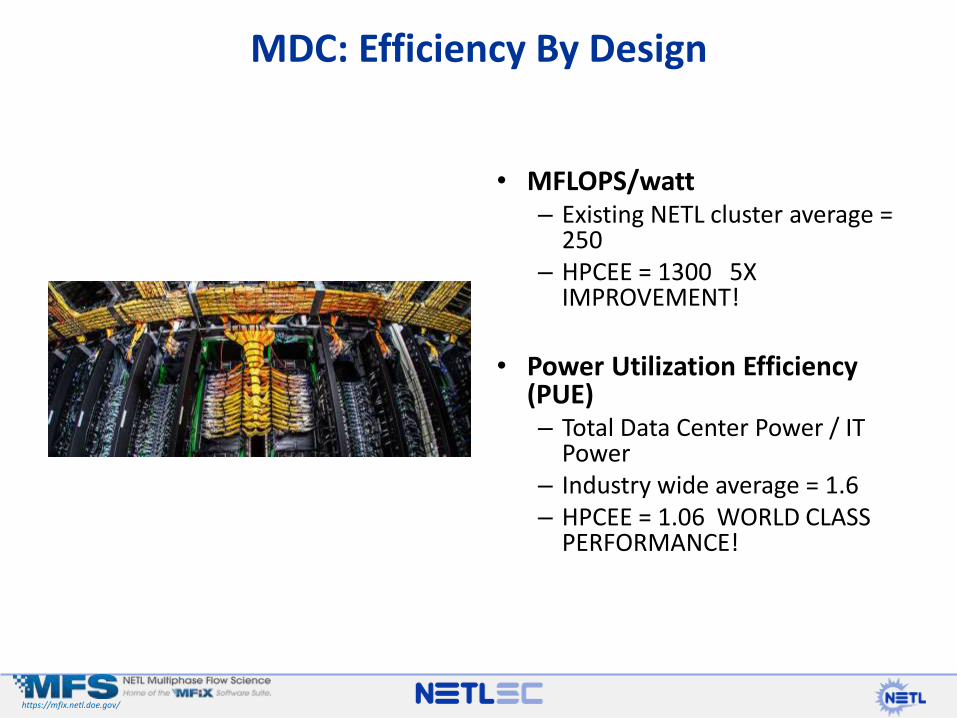
MDC: Efficiency By Design
• MFLOPS/watt– Existing NETL cluster average =
250– HPCEE = 1300 5X
IMPROVEMENT!
• Power Utilization Efficiency (PUE) – Total Data Center Power / IT
Power– Industry wide average = 1.6– HPCEE = 1.06 WORLD CLASS
PERFORMANCE!
https://mfix.netl.doe.gov/
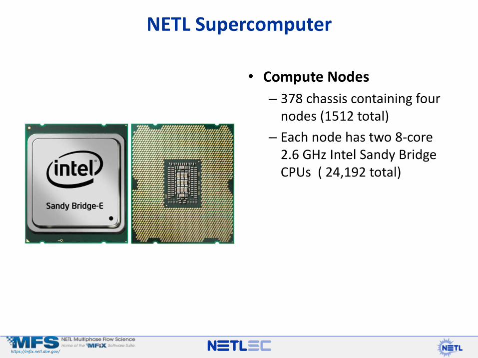
NETL Supercomputer
• Compute Nodes
– 378 chassis containing four nodes (1512 total)
– Each node has two 8-core 2.6 GHz Intel Sandy Bridge CPUs ( 24,192 total)
https://mfix.netl.doe.gov/
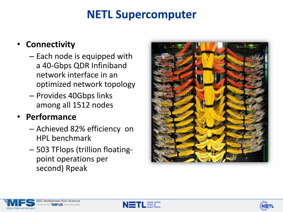
NETL Supercomputer
• Connectivity– Each node is equipped with
a 40-Gbps QDR Infiniband network interface in an optimized network topology
– Provides 40Gbps links among all 1512 nodes
• Performance– Achieved 82% efficiency on
HPL benchmark
– 503 TFlops (trillion floating-point operations per second) Rpeak
https://mfix.netl.doe.gov/
• Storage
– Total of 9 petabytes of disk storage
– 1 petabyte of primary disk storage attached to the compute nodes by Infiniband
– Storage is mirrored by an identical 1 petabyte array
• Software
– System runs Linux as the sole operating system.
– SUSE 11.4 is the current base distribution with specially compiled kernels to support parallel processing.
NETL Supercomputer
https://mfix.netl.doe.gov/
NETL Supercomputer
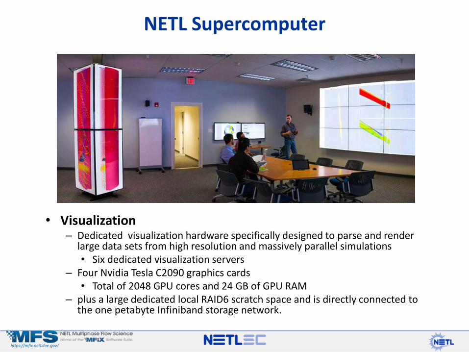
• Visualization– Dedicated visualization hardware specifically designed to parse and render
large data sets from high resolution and massively parallel simulations• Six dedicated visualization servers
– Four Nvidia Tesla C2090 graphics cards • Total of 2048 GPU cores and 24 GB of GPU RAM
– plus a large dedicated local RAID6 scratch space and is directly connected to the one petabyte Infiniband storage network.
https://mfix.netl.doe.gov/
High Performance Computing at NETL
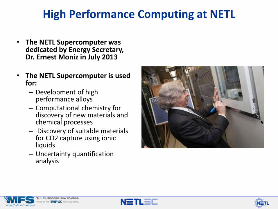
• The NETL Supercomputer was dedicated by Energy Secretary, Dr. Ernest Moniz in July 2013
• The NETL Supercomputer is used for:– Development of high
performance alloys– Computational chemistry for
discovery of new materials and chemical processes
– Discovery of suitable materials for CO2 capture using ionic liquids
– Uncertainty quantification analysis
https://mfix.netl.doe.gov/
• Motivation– There is a strong need to assess the credibility of numerical
prediction results for wider acceptance in development of new technologies for fossil fuel based clean energy.
– Verification, Validation and Uncertainty Quantification (VV&UQ) methods provide the required objective means in establishing the confidence level from simulation outcome.
• Objective– Determine the best set of methods, techniques and software
tools applicable for reactive multiphase flow simulation in order to access the uncertainty in simulation results
Uncertainty Quantification
https://mfix.netl.doe.gov/
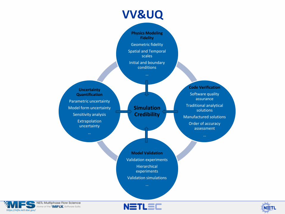
VV&UQ
Simulation Credibility
Physics Modeling Fidelity
Geometric fidelity
Spatial and Temporal scales
Initial and boundary conditions
…
Code Verification
Software quality assurance
Traditional analytical solutions
Manufactured solutions
Order of accuracy assessment
…
Model Validation
Validation experiments
Hierarchical experiments
Validation simulations
…
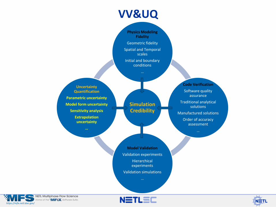
Uncertainty Quantification
Parametric uncertainty
Model form uncertainty
Sensitivity analysis
Extrapolation uncertainty
…
https://mfix.netl.doe.gov/
VV&UQ
Simulation Credibility
Physics Modeling Fidelity
Geometric fidelity
Spatial and Temporal scales
Initial and boundary conditions
…
Code Verification
Software quality assurance
Traditional analytical solutions
Manufactured solutions
Order of accuracy assessment
…
Model Validation
Validation experiments
Hierarchical experiments
Validation simulations
…
Uncertainty Quantification
Parametric uncertainty
Model form uncertainty
Sensitivity analysis
Extrapolation uncertainty
…
https://mfix.netl.doe.gov/
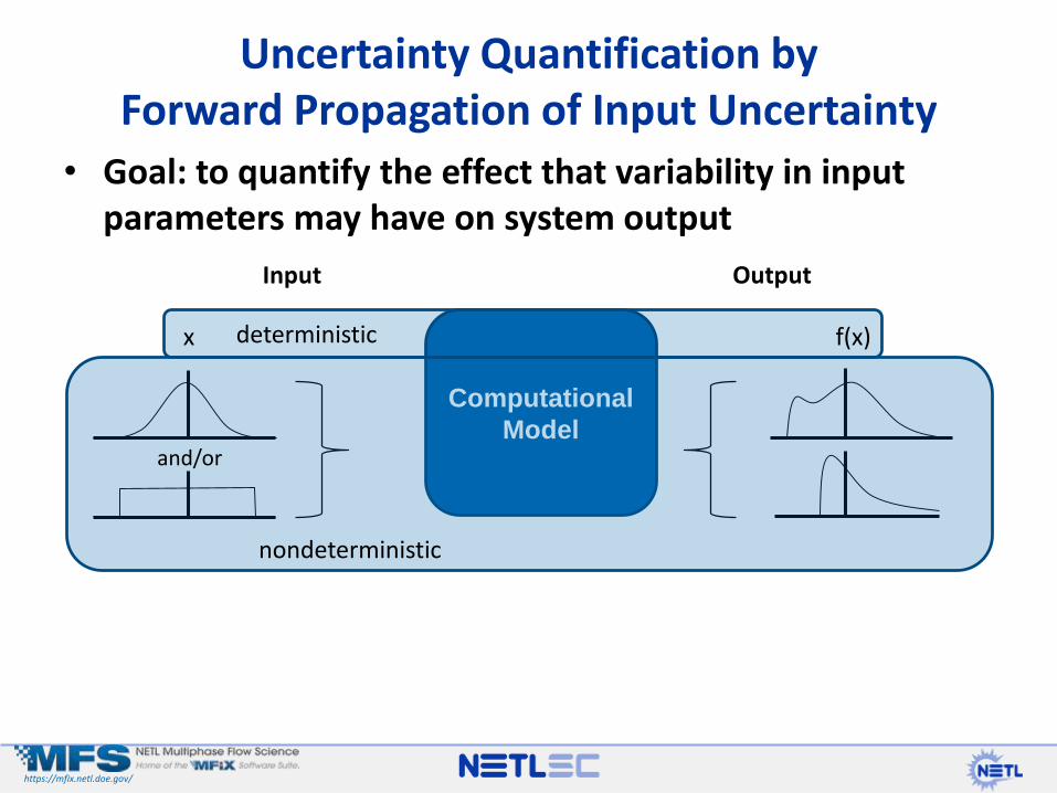
• Goal: to quantify the effect that variability in input parameters may have on system output
Uncertainty Quantification by Forward Propagation of Input Uncertainty
x f(x)deterministic
Input Output
Computational
Model
nondeterministic
and/or
https://mfix.netl.doe.gov/
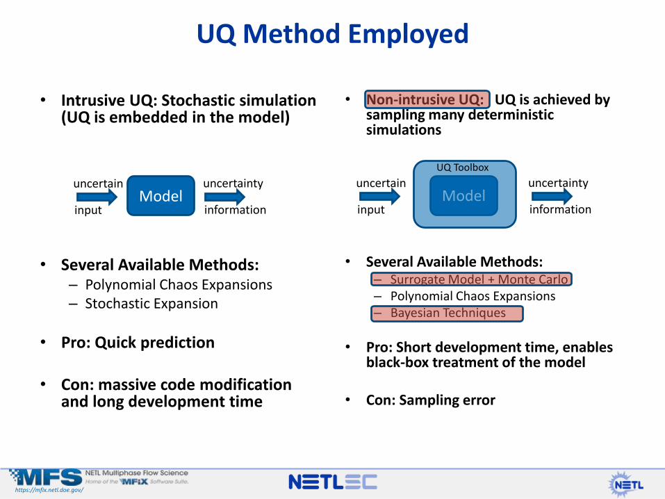
UQ Method Employed
• Intrusive UQ: Stochastic simulation (UQ is embedded in the model)
• Several Available Methods:– Polynomial Chaos Expansions– Stochastic Expansion
• Pro: Quick prediction
• Con: massive code modification and long development time
• Non-intrusive UQ: UQ is achieved by sampling many deterministic simulations
• Several Available Methods:– Surrogate Model + Monte Carlo– Polynomial Chaos Expansions– Bayesian Techniques
• Pro: Short development time, enables black-box treatment of the model
• Con: Sampling error
uncertain uncertaintyModel
input information
uncertain uncertaintyModel
input information
UQ Toolbox
https://mfix.netl.doe.gov/
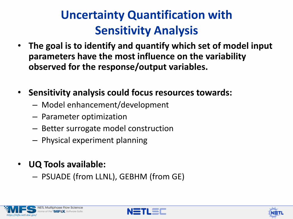
• The goal is to identify and quantify which set of model input parameters have the most influence on the variability observed for the response/output variables.
• Sensitivity analysis could focus resources towards:– Model enhancement/development
– Parameter optimization
– Better surrogate model construction
– Physical experiment planning
• UQ Tools available: – PSUADE (from LLNL), GEBHM (from GE)
Uncertainty Quantification with Sensitivity Analysis
https://mfix.netl.doe.gov/
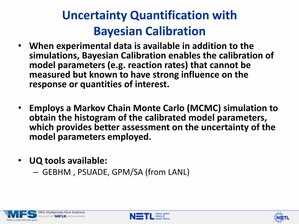
• When experimental data is available in addition to the simulations, Bayesian Calibration enables the calibration of model parameters (e.g. reaction rates) that cannot be measured but known to have strong influence on the response or quantities of interest.
• Employs a Markov Chain Monte Carlo (MCMC) simulation to obtain the histogram of the calibrated model parameters, which provides better assessment on the uncertainty of the model parameters employed.
• UQ tools available:– GEBHM , PSUADE, GPM/SA (from LANL)
Uncertainty Quantification withBayesian Calibration
https://mfix.netl.doe.gov/
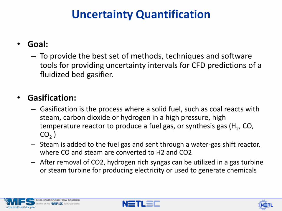
• Goal:– To provide the best set of methods, techniques and software
tools for providing uncertainty intervals for CFD predictions of a fluidized bed gasifier.
• Gasification:– Gasification is the process where a solid fuel, such as coal reacts with
steam, carbon dioxide or hydrogen in a high pressure, high temperature reactor to produce a fuel gas, or synthesis gas (H2, CO, CO2 )
– Steam is added to the fuel gas and sent through a water-gas shift reactor, where CO and steam are converted to H2 and CO2
– After removal of CO2, hydrogen rich syngas can be utilized in a gas turbine or steam turbine for producing electricity or used to generate chemicals
Uncertainty Quantification
https://mfix.netl.doe.gov/
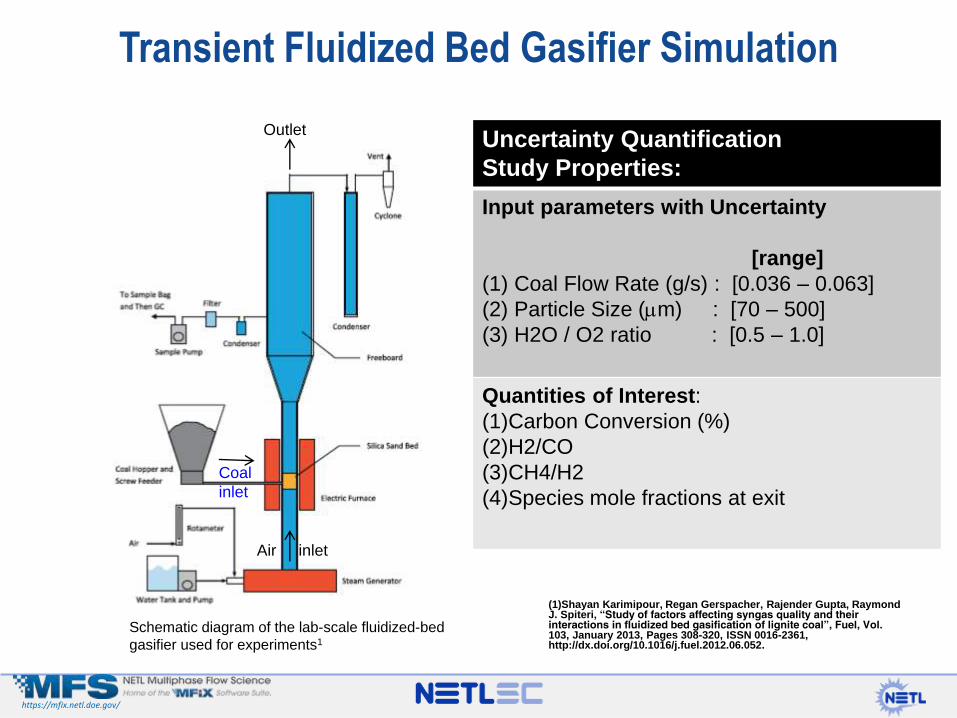
Transient Fluidized Bed Gasifier Simulation
(1)Shayan Karimipour, Regan Gerspacher, Rajender Gupta, Raymond J. Spiteri, “Study of factors affecting syngas quality and their interactions in fluidized bed gasification of lignite coal”, Fuel, Vol. 103, January 2013, Pages 308-320, ISSN 0016-2361, http://dx.doi.org/10.1016/j.fuel.2012.06.052.
Schematic diagram of the lab-scale fluidized-bed
gasifier used for experiments1
Coal
inlet
Outlet
Air inlet
Uncertainty Quantification
Study Properties:
Input parameters with Uncertainty
[range]
(1) Coal Flow Rate (g/s) : [0.036 – 0.063]
(2) Particle Size (mm) : [70 – 500]
(3) H2O / O2 ratio : [0.5 – 1.0]
Quantities of Interest:
(1)Carbon Conversion (%)
(2)H2/CO
(3)CH4/H2
(4)Species mole fractions at exit
https://mfix.netl.doe.gov/
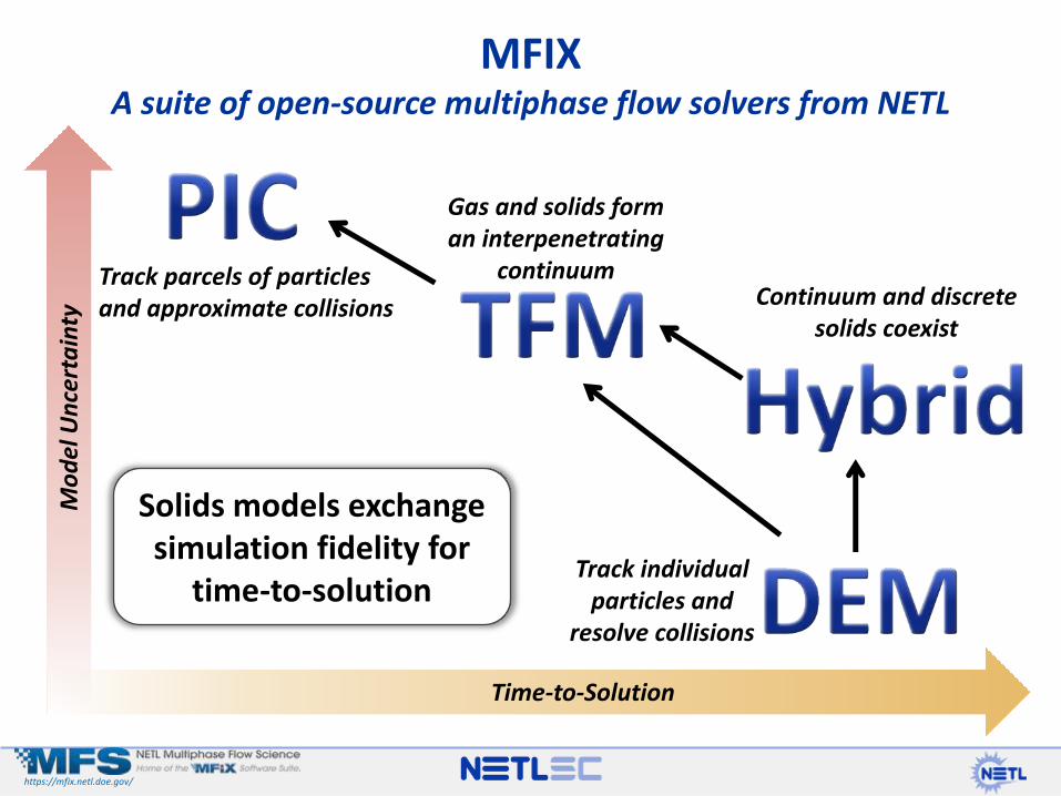
MFIXA suite of open-source multiphase flow solvers from NETL
Time-to-Solution
Mo
del
Un
cert
ain
ty
Track parcels of particlesand approximate collisions
Gas and solids form an interpenetrating
continuum
Track individual particles and
resolve collisions
Continuum and discrete solids coexist
Solids models exchange simulation fidelity for
time-to-solution
https://mfix.netl.doe.gov/
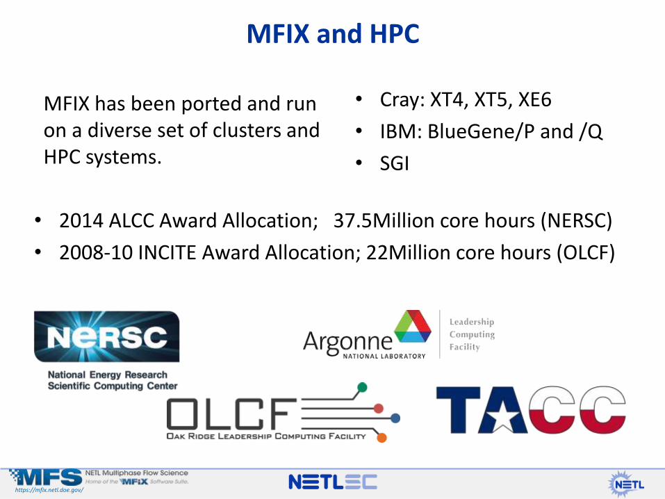
MFIX has been ported and run on a diverse set of clusters and HPC systems.
• 2014 ALCC Award Allocation; 37.5Million core hours (NERSC)
• 2008-10 INCITE Award Allocation; 22Million core hours (OLCF)
• Cray: XT4, XT5, XE6
• IBM: BlueGene/P and /Q
• SGI
MFIX and HPC
https://mfix.netl.doe.gov/
• Transient CFD simulations performed with MFIX-TFM.
• Coal pyrolysis, combustion, steam & CO2 gasification along with H2, CO and CH4 oxidation are modeled using 11 chemical reactions.
• Total of 33 transport equations are simultaneously solved for transport of 21 species and three phases (gas, coal and sand).
• Computational cost per simulation:– 2D : 2~3 weeks on 16 cores– 3D (30x350x30) : 7~8 weeks on 96 cores
Transient Fluidized Bed Gasifier Simulation
https://mfix.netl.doe.gov/
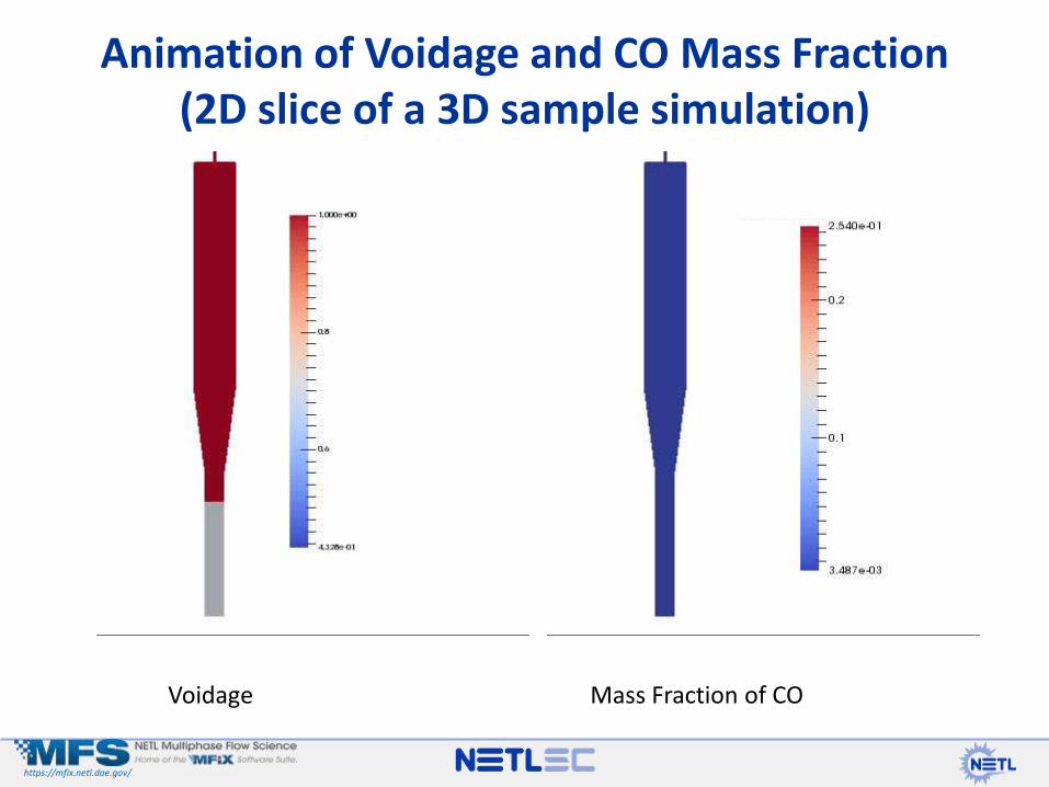
Animation of Voidage and CO Mass Fraction (2D slice of a 3D sample simulation)
Voidage Mass Fraction of CO
https://mfix.netl.doe.gov/
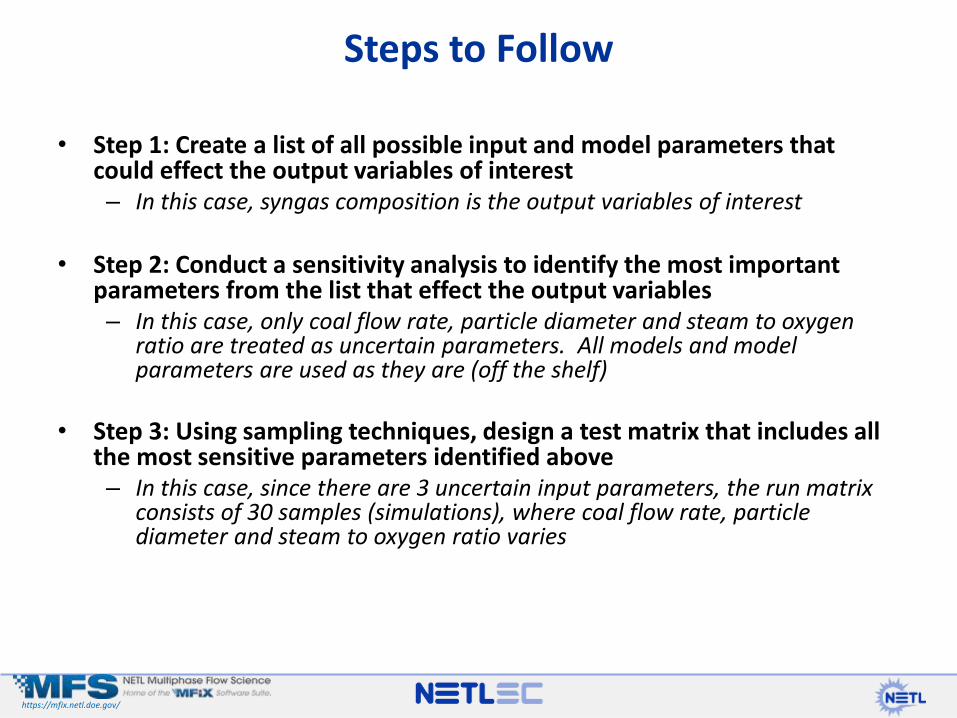
• Step 1: Create a list of all possible input and model parameters that could effect the output variables of interest– In this case, syngas composition is the output variables of interest
• Step 2: Conduct a sensitivity analysis to identify the most important parameters from the list that effect the output variables – In this case, only coal flow rate, particle diameter and steam to oxygen
ratio are treated as uncertain parameters. All models and model parameters are used as they are (off the shelf)
• Step 3: Using sampling techniques, design a test matrix that includes all the most sensitive parameters identified above– In this case, since there are 3 uncertain input parameters, the run matrix
consists of 30 samples (simulations), where coal flow rate, particle diameter and steam to oxygen ratio varies
Steps to Follow
https://mfix.netl.doe.gov/
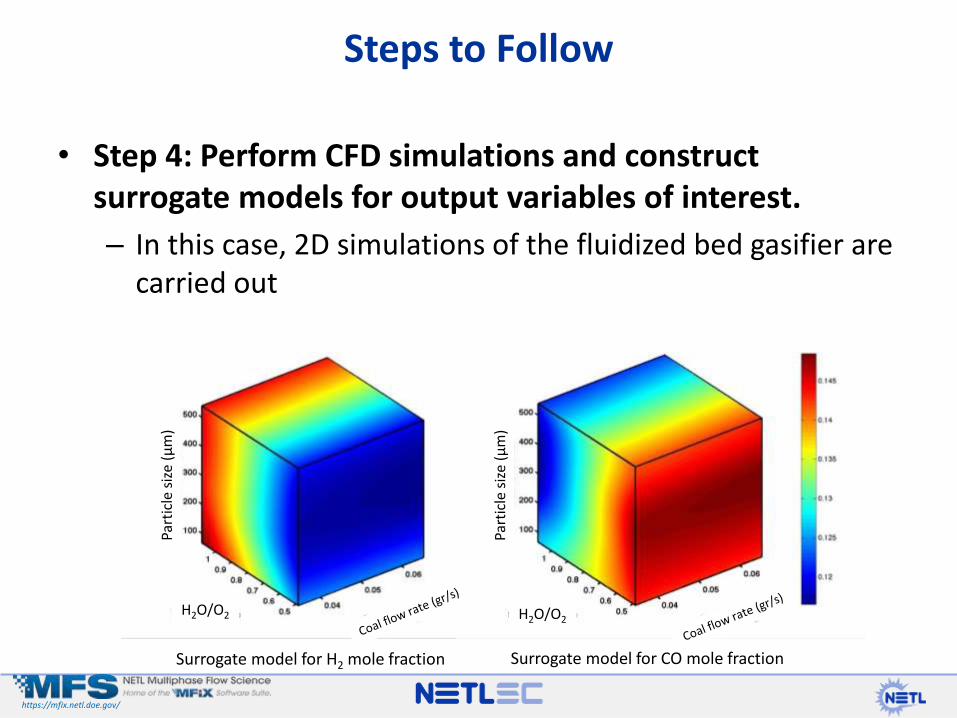
• Step 4: Perform CFD simulations and construct surrogate models for output variables of interest.
– In this case, 2D simulations of the fluidized bed gasifier are carried out
Steps to Follow
Surrogate model for H2 mole fraction Surrogate model for CO mole fraction
Part
icle
siz
e (µ
m)
Part
icle
siz
e (µ
m)
H2O/O2 H2O/O2
https://mfix.netl.doe.gov/
• Step 5: conduct Monte Carlo sampling of the surrogate models to construct distribution functions for the quantities of interest, as a function of the uncertain input parameters
– In this case, construct distribution functions for CO and H2
mole fraction at the exit plane of the gasifier, as coal flow rate, coal particle diameter and H2O/O2 vary
Steps to Follow
https://mfix.netl.doe.gov/
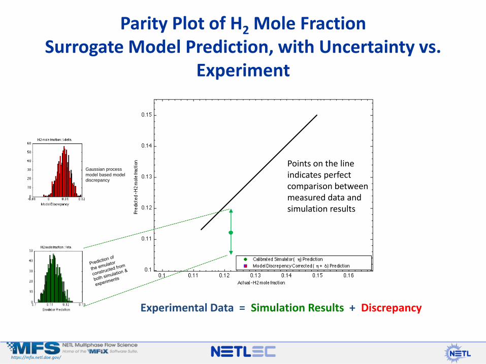
Parity Plot of H2 Mole Fraction Surrogate Model Prediction, with Uncertainty vs.
Experiment
Gaussian process
model based model
discrepancy
Points on the line indicates perfect comparison between measured data and simulation results
Experimental Data = Simulation Results + Discrepancy

https://mfix.netl.doe.gov/
Parity Plot of H2 Mole Fraction Surrogate Model Prediction, with Uncertainty,
Corrected for Model Discrepancy vs. Experiment
Experimental Data = Simulation Results + Discrepancy
https://mfix.netl.doe.gov/
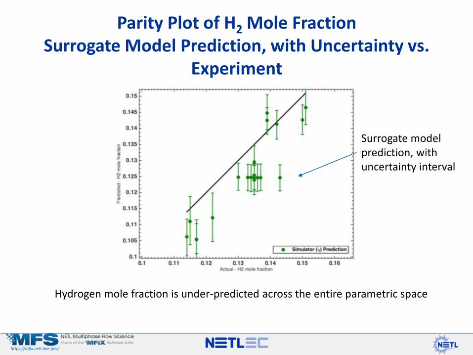
Parity Plot of H2 Mole Fraction Surrogate Model Prediction, with Uncertainty vs.
Experiment
Hydrogen mole fraction is under-predicted across the entire parametric space
Surrogate model prediction, with uncertainty interval
https://mfix.netl.doe.gov/
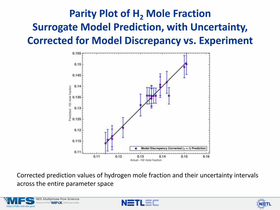
Parity Plot of H2 Mole Fraction Surrogate Model Prediction, with Uncertainty,
Corrected for Model Discrepancy vs. Experiment
Corrected prediction values of hydrogen mole fraction and their uncertainty intervals across the entire parameter space
https://mfix.netl.doe.gov/
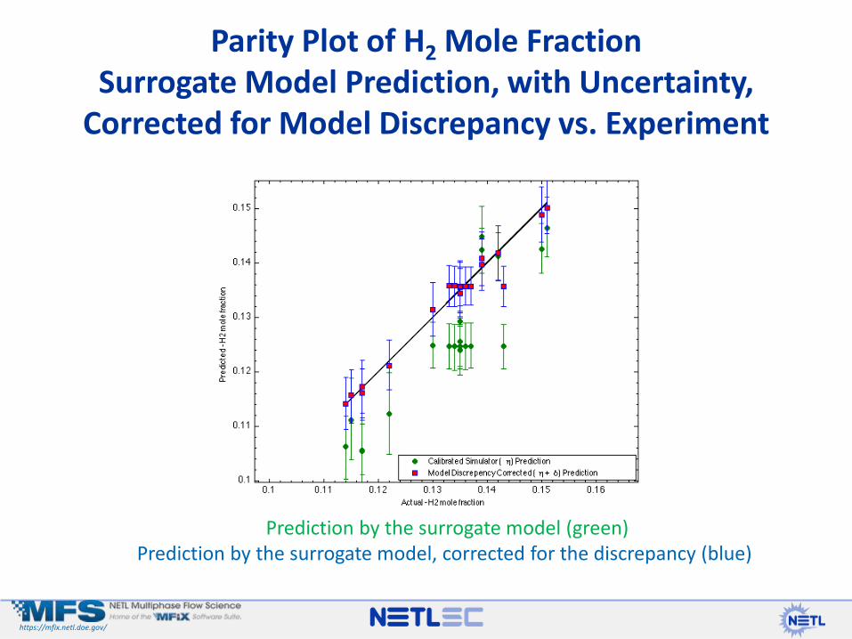
Parity Plot of H2 Mole Fraction Surrogate Model Prediction, with Uncertainty,
Corrected for Model Discrepancy vs. Experiment
Prediction by the surrogate model (green)Prediction by the surrogate model, corrected for the discrepancy (blue)
https://mfix.netl.doe.gov/
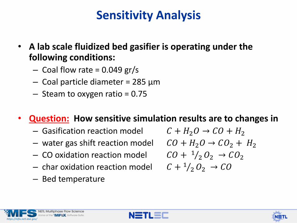
• A lab scale fluidized bed gasifier is operating under the following conditions:– Coal flow rate = 0.049 gr/s
– Coal particle diameter = 285 µm
– Steam to oxygen ratio = 0.75
• Question: How sensitive simulation results are to changes in– Gasification reaction model 𝐶 + 𝐻2𝑂 → 𝐶𝑂 + 𝐻2
– water gas shift reaction model 𝐶𝑂 + 𝐻2𝑂 → 𝐶𝑂2 + 𝐻2
– CO oxidation reaction model 𝐶𝑂 + 1 2𝑂2 → 𝐶𝑂2– char oxidation reaction model 𝐶 + 1 2𝑂2 → 𝐶𝑂
– Bed temperature
Sensitivity Analysis
https://mfix.netl.doe.gov/
• A test matrix comprising of 50 samples is constructed with Optimal Latin Hypercube Sampling, where
– The gasification rate varies
– Two different CO and char oxidation models are tested
– Catalytic vs. non-catalytic water gas shift reaction is tested
– Bed temperature varies between [790 – 810] C
• 50 x 3D transient CFD simulations are conducted and surrogate models for the Quantities of Interest (QoI) are constructed using the results obtained.
Sensitivity Analysis
https://mfix.netl.doe.gov/
Sensitivity Analysis
0
10
20
30
40
50
60
70
80
90
100
Water Gas Shift Reaction Gasification reaction Bed Temperature CO Oxidation Reaction Char Oxidation Reaction
CO H2 CO2
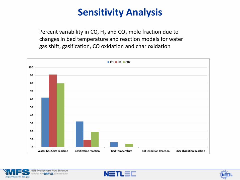
Percent variability in CO, H2 and CO2 mole fraction due to changes in bed temperature and reaction models for water gas shift, gasification, CO oxidation and char oxidation
https://mfix.netl.doe.gov/
Surrogate Models Can Provide Insight in Trends
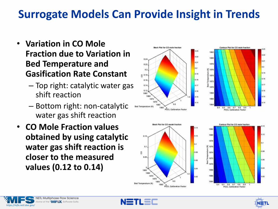
• Variation in CO Mole Fraction due to Variation in Bed Temperature and Gasification Rate Constant– Top right: catalytic water gas
shift reaction
– Bottom right: non-catalytic water gas shift reaction
• CO Mole Fraction values obtained by using catalytic water gas shift reaction is closer to the measured values (0.12 to 0.14)
https://mfix.netl.doe.gov/
Surrogate Models Can Provide Insight in Trends
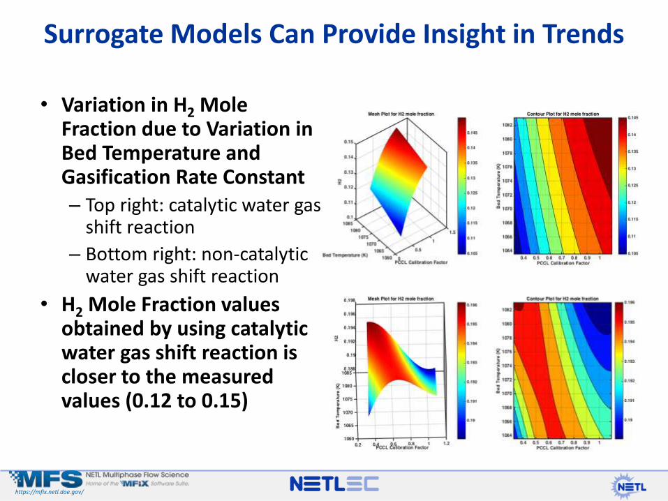
• Variation in H2 Mole Fraction due to Variation in Bed Temperature and Gasification Rate Constant– Top right: catalytic water gas
shift reaction
– Bottom right: non-catalytic water gas shift reaction
• H2 Mole Fraction values obtained by using catalytic water gas shift reaction is closer to the measured values (0.12 to 0.15)
https://mfix.netl.doe.gov/
• Bayesian Uncertainty Quantification analysis provided uncertainty intervals for the CFD simulation results in the parametric space tested.
• Sensitivity Analysis points to the water gas shift reaction as being the most important reaction in effecting the syngas composition (CO and H2)
• Based on analysis of the surrogate models for CO and H2, the catalytic water gas shift reaction is the suitable reaction to use for conversion of CO to H2.
• Sensitivity analysis shows that improvements in the catalytic water gas shift reaction model, gasification reaction model and heat transfer between gas and solid phases can lead to improvement in model prediction
Conclusions
https://mfix.netl.doe.gov/
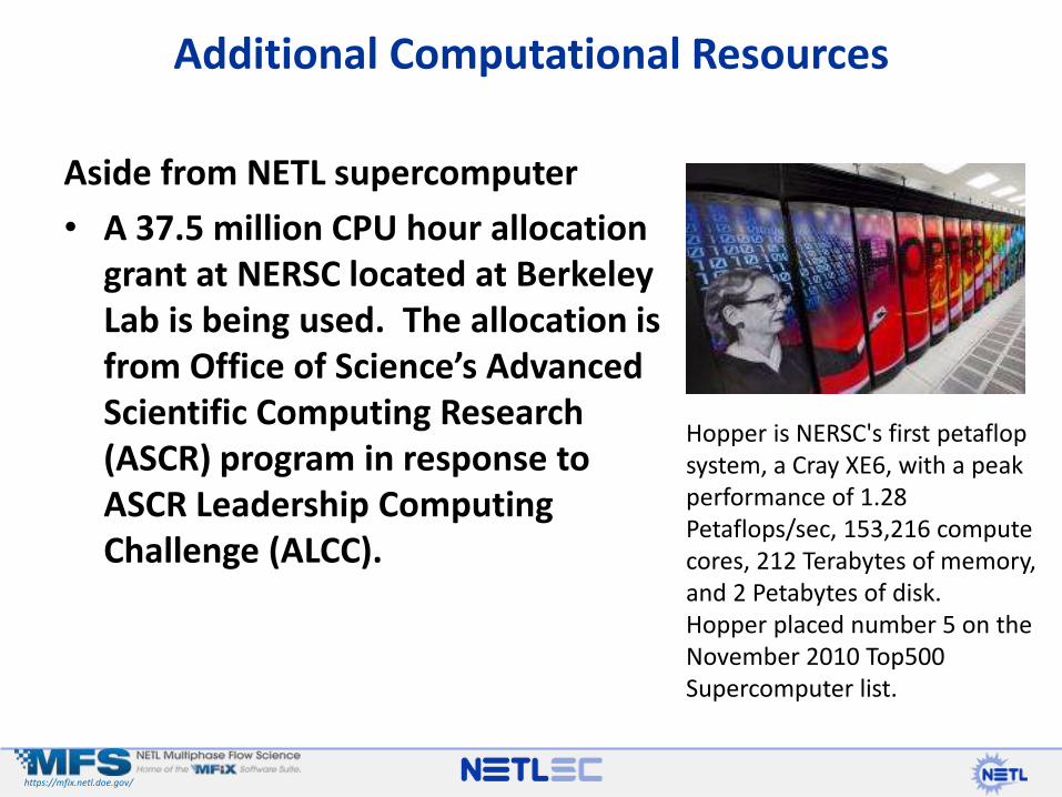
Aside from NETL supercomputer
• A 37.5 million CPU hour allocation grant at NERSC located at Berkeley Lab is being used. The allocation is from Office of Science’s Advanced Scientific Computing Research (ASCR) program in response to ASCR Leadership Computing Challenge (ALCC).
Additional Computational Resources
Hopper is NERSC's first petaflopsystem, a Cray XE6, with a peak performance of 1.28 Petaflops/sec, 153,216 compute cores, 212 Terabytes of memory, and 2 Petabytes of disk. Hopper placed number 5 on the November 2010 Top500 Supercomputer list.