High-dimensional variable selection by decorrelation ... · II. The CAR-score III. Results IV. Conclusion High-dimensional variable selection by decorrelation: Introducing the CAR-score

I. The Linear ModelII. The CAR-score

III. ResultsIV. Conclusion

High-dimensional variable selection by

decorrelation:

Introducing the CAR-score

Verena Zuber

joint work withKorbinian Strimmer

Institut für Medizinische Informatik, Statistik und Epidemiologie(IMISE), University of Leipzig

Workshop on

Validation in Statistics and Machine Learning

Oktober 6th, 2010Verena Zuber High-dimensional feature selection 1/27



�It is a very sad thing that nowadaysthere is so little useless information.�

Oscar Wilde

published in Saturday Review (1894)

Today: Analysis of gene-expression data?

p = 11 940 genes

After analysis

p = 462 interesting genes

? Lu et al. (2004): � Gene regulation and DNA damage in the ageing human brain�

Verena Zuber High-dimensional feature selection 2/27



The linear modelVariable selection in the linear model

I. The Linear Model:Focus on Variable Selection and Importance





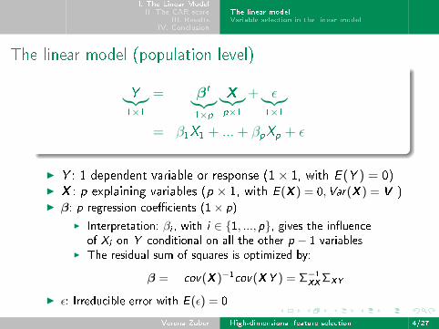
The linear model (population level)

Y︸︷︷︸1×1

= βt︸︷︷︸1×p

X︸︷︷︸p×1

+ ε︸︷︷︸1×1

= β1X1 + ...+ βpXp + ε

I Y : 1 dependent variable or response (1× 1, with E (Y ) = 0)I X : p explaining variables (p × 1, with E (X ) = 0,Var(X ) = V )I β: p regression coe�cients (1× p)

I Interpretation: βi , with i ∈ {1, ..., p}, gives the in�uenceof Xi on Y conditional on all the other p − 1 variables

I The residual sum of squares is optimized by:

β = cov(X )−1cov(XY ) = Σ−1XXΣXY

I ε: Irreducible error with E (ε) = 0





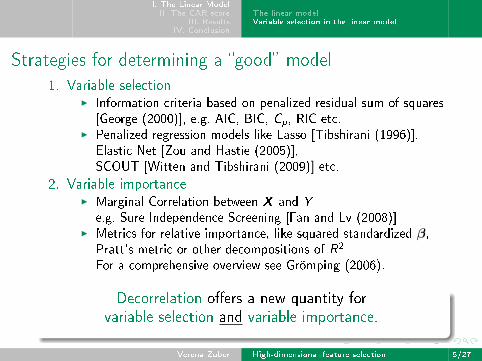
Strategies for determining a �good� model1. Variable selection

I Information criteria based on penalized residual sum of squares[George (2000)], e.g. AIC, BIC, Cp, RIC etc.

I Penalized regression models like Lasso [Tibshirani (1996)],Elastic Net [Zou and Hastie (2005)],SCOUT [Witten and Tibshirani (2009)] etc.

2. Variable importanceI Marginal Correlation between X and Y

e.g. Sure Independence Screening [Fan and Lv (2008)]I Metrics for relative importance, like squared standardized β,

Pratt's metric or other decompositions of R2

For a comprehensive overview see Grömping (2006).

Decorrelation o�ers a new quantity forvariable selection and variable importance.




Presenting the CAR-scoreProperties of the CAR-scoreThe CAR-score in practice

How decorrelation leads to a new tool

for variable selection and quantifying variable importance:

II. Presenting Correlation Adjusted CoRRelation,the CAR-score





De�nition of the CAR-score

We de�ne the p-dimensional CAR-score vector

(Correlation Adjusted CoRRelation) ω as:

ω︸︷︷︸p×1

= P−1/2︸︷︷︸p×p

PXY︸︷︷︸p×1

I P: Correlation of X

I PXY : Vector of marginal correlations between X and Y

Criterion for variable importance:

We propose to use ω2(i) to quantify the importance

of variable Xi in the linear model, with i ∈ 1, ..., p





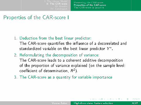
Properties of the CAR-score I

1. Deduction from the best linear predictor:

The CAR-score quanti�es the in�uence of a decorrelated and

standardized variable on the best linear predictor Y ?.

2. Reformulating the decomposition of variance:

The CAR-score leads to a coherent additive decomposition

of the proportion of variance explained (on the sample level:

coe�cient of determination, R2).

3. The CAR-score as a quantity for variable importance





1. The best linear predictorY ? = βt︸︷︷︸

ΣtXY

Σ−1XX

X

After some simple transformations the standardized best linear

predictor Y ? simpli�es to the following decomposition:

Y ?/σY = ωt δ(X )

I The decorrelated and standardized data δ(X ); Cov(δ(X )) = diag(1)

δ(X)︸︷︷︸

p×1

= P−1/2

V−1/2

X

I The correlation between X and Y adjusted for the correlation

among X :

ω︸︷︷︸p×1

= P−1/2

PXY





2. Decomposition of the proportion of variance explained

I Total variance: Var(Y ) = σ2YI Explained variance:

Var(Y ?) = σ2YVar(ωtδ(X ))

= σ2Yωt Var(δ(X ))︸︷︷︸

diag(1)

ω

= σ2Yωtω

I The decomposition of variance rewritten in CAR-scores:

Total variance︷︸︸︷Var(Y ) =

Explained variance︷︸︸︷Var(Y ?) +

Unexplained variance︷︸︸︷Var(Y − Y ?)

σ2Y = σ2Y (ωtω) + σ2Y (1− ωtω)





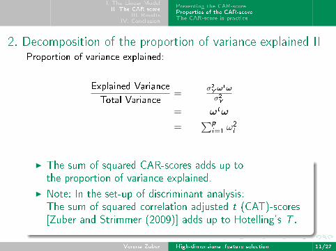
2. Decomposition of the proportion of variance explained IIProportion of variance explained:

Explained Variance

Total Variance=

σ2Yωtω

σ2Y

= ωtω

=∑p

i=1 ω2i

I The sum of squared CAR-scores adds up tothe proportion of variance explained.

I Note: In the set-up of discriminant analysis:The sum of squared correlation adjusted t (CAT)-scores[Zuber and Strimmer (2009)] adds up to Hotelling's T .





3. The CAR-score as quantity for variable importance

1. Proper decomposition of the proportion of variance explained:

Explained Variance

Total Variance=

p∑i=1

ω2i

2. Non-negativity: ω2i ≥ 0

3. Inclusion-Property: ω2i 6= 0 if βi 6= 0

4. Exclusion-Property: ω2i = 0 if βi = 0

The CAR-score ful�lls the Exclusion-Property only

if there is no correlation between the null variables with β = 0

and non-null variables with β 6= 0





Properties of the CAR-score II

4. Connections to other quantities for variable importance:

Correlation︷︸︸︷PXY

P−1/2→

CAR-score︷︸︸︷P−1/2

PXY = ωP−1/2→

Std. Regression Coe�.︷︸︸︷P−1/2ω = βstd

5. Oracle CAR-score: If we know

I which variables are null or non-null andI that there is no correlation between null and non-null variables

then any consistent estimate of the CAR-score ω = P1/2βstd

equals 0 for the null variables:

ω =

(Pnon-null 0

0 Pnull

)1/2

︸︷︷︸P1/2

(βstd,non-null

0

)︸︷︷︸

βstd

=

(ωnon-null

0

)





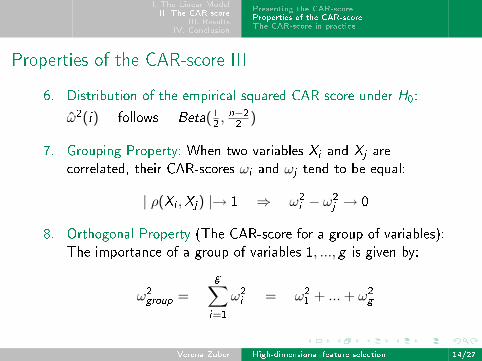
Properties of the CAR-score III

6. Distribution of the empirical squared CAR-score under H0:

ω̂2(i) follows Beta(12 ,n−22 )

7. Grouping Property: When two variables Xi and Xj are

correlated, their CAR-scores ωi and ωj tend to be equal:

| ρ(Xi ,Xj) |→ 1 ⇒ ω2i − ω2

j → 0

8. Orthogonal Property (The CAR-score for a group of variables):

The importance of a group of variables 1, ..., g is given by:

ω2group =

g∑i=1

ω2i = ω2

1 + ...+ ω2g





The CAR-score is a population quantity;thus it is not tied to any inference framework.Any kind of �good� estimate can be used.

A simple recipe for variable selection:

1. (If p is too large, a prescreening is advisable.

Limitation: Estimation of the p × p correlation matrix P)

2. Estimate the CAR-scores:I Large sample case (n >> p): Empirical estimatesI Small n, large p: Regularized estimates, like shrinkage

procedures or penalized maximum likelihood estimates

3. Rank the variables according to their squared CAR-score

4. Choose a suitable cut-o� (a �xed cut-o� corresponds

to information criteria like AIC, BIC, etc)

5. Re�t the linear model based on the remaining variables




SimulationAnalysis of benchmark data

IV. Results

All analysis is performed in R

I care: Empirical and shrinkage estimates for the CAR-scoreI relaimpo: Relative importance of variablesI scout: Implementation of Lasso and Elastic NetI fdrtool: False (non) discovery rate





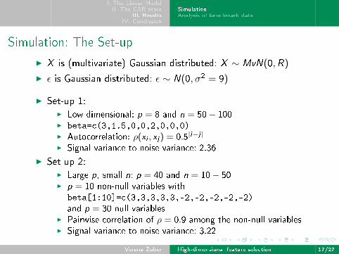
Simulation: The Set-up

I X is (multivariate) Gaussian distributed: X ∼ MvN(0,R)

I ε is Gaussian distributed: ε ∼ N(0, σ2 = 9)

I Set-up 1:I Low dimensional: p = 8 and n = 50− 100I beta=c(3,1.5,0,0,2,0,0,0)I Autocorrelation: ρ(xi , xj) = 0.5|i−j|

I Signal variance to noise variance: 2.36

I Set-up 2:I Large p, small n: p = 40 and n = 10− 50I p = 10 non-null variables with

beta[1:10]=c(3,3,3,3,3,-2,-2,-2,-2,-2)

and p = 30 null variablesI Pairwise correlation of ρ = 0.9 among the non-null variablesI Signal variance to noise variance: 3.22





Simulation: Comparing the results

I What to compare?

1. Variable selection:Mean model error, median model size and the β-coe�cients

2. Variable importance:Quantity of the di�erent metrics

I The competitors:

1. Variable selection:Elastic Net, Lasso and Ordinary Least Squares

2. Variable importance:Squared βstd's, Pratt's measure and the lmg-measure

I Set-up 1: Empirical CAR-score; Set-up 2: Shrinkage CAR-score

I The CAR-scores are used for variable selection,

then the linear model is re�tted





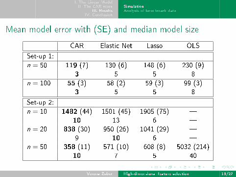
Mean model error with (SE) and median model size

CAR Elastic Net Lasso OLS

Set-up 1:

n = 50 119 (7) 130 (6) 148 (6) 230 (9)

3 5 5 8

n = 100 55 (3) 58 (2) 59 (3) 99 (3)

3 5 5 8

Set-up 2:

n = 10 1482 (44) 1501 (45) 1905 (75) �

10 13 6 �

n = 20 838 (30) 950 (26) 1041 (29) �

9 10 6 �

n = 50 358 (11) 571 (10) 608 (8) 5032 (214)

10 7 5 40





Set-up 1: Boxplots of the estimated variable importancebeta=c(3,1.5,0,0,2,0,0,0)

1 2 3 4 5 6 7 8

−0.

20.

00.

20.

40.

60.

8

pratt

Number of Variable

Var

iabl

e Im

port

ance

1 2 3 4 5 6 7 8

−0.

20.

00.

20.

40.

60.

8

lmg

Number of Variable

Var

iabl

e Im

port

ance

1 2 3 4 5 6 7 8

−0.

20.

00.

20.

40.

60.

8

betasq

Number of Variable

Var

iabl

e Im

port

ance

1 2 3 4 5 6 7 8

−0.

20.

00.

20.

40.

60.

8

car

Number of Variable

Var

iabl

e Im

port

ance





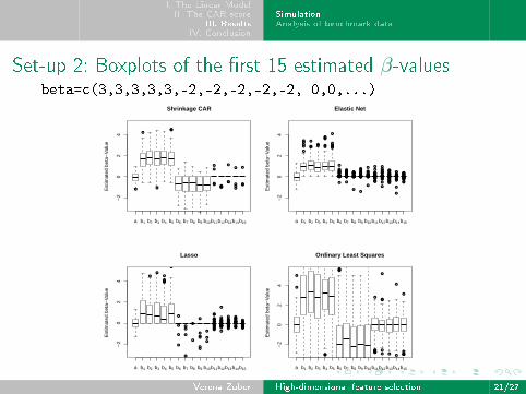
Set-up 2: Boxplots of the �rst 15 estimated β-valuesbeta=c(3,3,3,3,3,-2,-2,-2,-2,-2, 0,0,...)

●

●

●

●●

●

●

●

●

●●●

●

●

●

●

●

●●

●

●

●

a b1 b2 b3 b4 b5 b6 b7 b8 b9 b10b11b12b13b14b15

−2

02

4

Shrinkage CARE

stim

ated

bet

a−V

alue

●●●

●

●

●

●●●● ●

●

●

●●

●●●

●

●●

●●

●

●●●

●●

●

●●

●●●●●●●

●

●●●●●●●●

●

●

●●●●

●

●●

●

●

●●

●

●●

●

●●

●●

●●●●●●●

●

●●●●

●●●●●

●

●●●●

●

●●

●●

●

●●●●●

●

●●●●●●●

●

●●

●●

●

●

●●●●●●●●

●

●●●●●●

●

●●●

●

●

●●

●

●

●

●●●●

●●●

●

●

●

●

●●

●

●

●●

●

●

●

●●

●

●●

●

●

●

●

●

●

●●

●

●●

●●

●

●

●●●●●

●

●●●●●

●

●

●●

●

●

●●●

●

●

●

●●●●

●

●●

●●

●●

●●

●●●

●

●●●●●●

●

●●●

●●●

●

●●


−2

02

4

Elastic Net

Est

imat

ed b

eta−

Val

ue

●

●

●

●●●

●

●

●

●

●

●

●

●

●

●

●

●

●

●●

●●

●

●

●

●

●

●

●

●●

●●

●

●●●

●

●

●●

●●

●●●

●●

●●●

●

●

●

●

●●

●

●

●

●

●

●

●

●

●●●

●●

●

●

●●

●

●●●

●

●

●●●

●

●

●

●

●●

●●

●●

●

●●●●●●

●

●

●●

●●●●

●●

●●


−2

02

4

Lasso

Est

imat

ed b

eta−

Val

ue

●

●

●

●

● ●

●

●

●

●

●

●

●

●

●

●

●

●

●

●

●

●

●

●●

●●

●

●

●

●

●

●

●

●

●●●●● ●

●

●

●

●

●

●

●

●

●●

●

●●


−2

02

4

Ordinary Least Squares

Est

imat

ed b

eta−

Val

ue





�Gene regulation and DNA damage in the ageing human brain�

from Lu et al. in Nature (2004)

I The data is available on the Gene Expression Omnibus

(�GSE1572�)

I n = 30 and p = 12 625

I Y : Age of the individual (26-106 years)

I X : Gene expression of postmortem brain tissue (frontal cortex)

(Platform: A�ymetrix Human Genome U95 Version 2 Array)

I A prescreening is performed using the empirical marginal

correlations and FNDR control: Remaining size p = 403

I Model size of the competing procedures:I Lasso: 36 genesI Elastic Net: 85 genesI CAR-score: 50− 60 genes

I All procedures include di�erent variables.





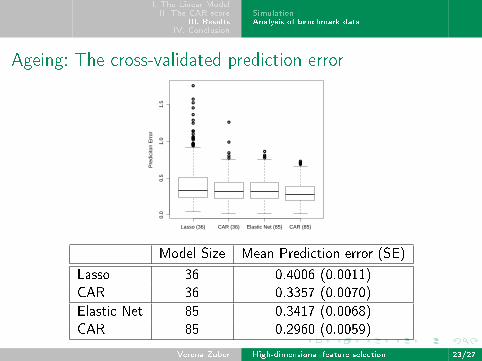
Ageing: The cross-validated prediction error

●

●

●

●

●

●

●●

●

●

●

●

●

●●●

●

●

●

●

●

●

●

●

●

●●

●●●

●●●●

Lasso (36) CAR (36) Elastic Net (85) CAR (85)

0.0

0.5

1.0

1.5

Pre

dici

ton

Err

or

Model Size Mean Prediction error (SE)

Lasso 36 0.4006 (0.0011)

CAR 36 0.3357 (0.0070)

Elastic Net 85 0.3417 (0.0068)

CAR 85 0.2960 (0.0059)




IV. Conclusion




Summary

1. We introduce a remarkable simple way of quantifying variable

importance and selecting variables in the linear model:

The CAR-score

2. The CAR-score is embedded elegantly in thetheoretical framework of the linear model:

I The CAR-score quanti�es the in�uence of adecorrelated variable on the best linear predictor.

I It leads to a coherent decomposition ofthe proportion of variance explained.

3. Simulations show that the CAR-score achieves a

lower model error than Lasso and Elastic Net

and identi�es the correct model size.

4. In the analysis of real data the CAR-score achieves a

lower prediction error than competing procedures.




The preprint of Zuber and Strimmer (2010):

�Variable importance and model selection by decorrelation�

is available on:

I http://arxiv.org/abs/1007.5516

I http://www.uni-leipzig.de/~zuber/

care(CAR-Estimation)-package available from CRAN:

I cran.r-project.org/web/packages/care/index.html

Thank You Very MuchFor Your Attention!


http://arxiv.org/abs/1007.5516

http://www.uni-leipzig.de/~zuber/

cran.r-project.org/web/packages/care/index.html



I Fan and Li (2001): �Variable selection via nonconcave penalizedlikelihood and its oracle properties.� JASA (96) 1348-1360

I Fan and Lv (2008): �Sure Independence Screening for Ultra-HighDimensional Feature Space.� JRSS Series B (70) 849-911

I Grömping (2006): �Relative Importance for Linear Regression in R�Journal of Statistical Software 17 (1)

I Lu et al. (2004): � Gene regulation and DNA damage in the ageinghuman brain.� Nature (429) 883-891

I Tibshirani (1996): �Regression shrinkage and selection via thelasso.� JRSS Series B. (58) 267-288

I Witten and Tibshirani (2009): �Covariance-regularized regressionand classi�cation for high-dimensional problems.� JRSS Series B.

I Zou and Hastie (2005): �Regularization and variable selection viathe elastic net.� JRSS Series B. (67) 301-320

I Zuber and Strimmer (2009): �Gene ranking and biomarker discoveryunder correlation.� Bioinformatics (25) 2700-2707


Documents

High-dimensional variable selection by decorrelation ... · II. The CAR-score III. Results IV. Conclusion High-dimensional variable selection by decorrelation: Introducing the CAR-score