Mat-2.108 – Independent Research Project in Applied Mathematics

Hierarchical Preference Elicitation inRobust Portfolio Modeling

Antti Toppila 60719S

February 2, 2007

Helsinki University of TechnologyDepartment of Engineering Physics and MathematicsSystems Analysis Laboratory

1 INTRODUCTION

Contents

1 Introduction 1

2 Robust Portfolio Modeling 32.1 Multi-Criteria Project Portfolio selection . . . . . . . . . . . . 32.2 Modeling Incomplete Information . . . . . . . . . . . . . . . . 5

3 Value Trees 73.1 Structure of Value Trees . . . . . . . . . . . . . . . . . . . . . 73.2 Mathematical Treatment . . . . . . . . . . . . . . . . . . . . . 8

4 Software Implementation 12

5 Illustrative Example 13

6 Conclusions 18

1 Introduction

The selection of a project portfolio is a combinatorial problem where the

decision-maker (DM) has to choose the best projects from a set of candidate

projects. The projects have different strengths and weaknesses, and therefore

each project is evaluated with regard to two or more criteria (or attributes).

Possible portfolios are restricted by constraints such as a budget limitation,

for instance. Ideally, the selected portfolio performs in some sense best with

regard to all criteria. The final decision depends on the DM’s preferences.

As with all combinatorial problems, the solution space may become very

large, which results in difficulties if all possible portfolios are to be evaluated

separately. Another problem is that all necessary information does not exist

or cannot be produced in time or at a reasonable cost. This means that

it may be helpful to work with incomplete information. In addition, many

interdependencies among the projects can make it hard to limit the decision-

making process to feasible portfolios only. Yet, the DM should be able to

make a decision which can be subjected to critical inspection.

1

1 INTRODUCTION

There are numerous approaches to this problem. Golabi et al. (1981) de-

veloped an interactive procedure to assist in the selection of an R&D portfolio

of solar photovoltaic applications experiments posing some of the criteria as

minimum level constraints. This method is suitable when nonmonetary crite-

ria are accounted for. For instance, a strategic approach to allocating capital

in healthcare systems (Kleinmuntz et al., 1999) would make such considera-

tions necessary when dealing with soft values such as patient satisfaction or

quality of care.

Robust Portfolio Modeling (RPM, Liesio et al., 2006) supports project

portfolio selection in view of multiple criteria, incomplete information and

limited resources. It is developed for large scale problems with support for

incomplete information. This is necessary, as the decision-maker may not be

able to give complete preference information due to the very large number

of projects.

The method is based on finding non-dominated project portfolios: a port-

folio is non-dominated if no other portfolio is better for all possible realiza-

tions of feasible parameters. Projects that are included in all non-dominated

portfolios should always be selected (core projects). Conversely, projects

that are not included in any non-dominated portfolio should not be selected

(exterior projects). This allows the DM to focus on the remaining borderline

projects and to find new core and exterior projects by giving additional infor-

mation about the borderline projects, since new information can influence the

status of borderline projects only. This saves resources and enables quicker

results, as candidate projects can be completely eliminated each round.

Value trees (Keeney and Raiffa, 1976) are a common method for problem

structuring in multiple criteria decision-making by decomposing the problem

into smaller parts which can be evaluated separately. Also, in these methods

the DM must structure her objectives as a hierarchy of attributes (Belton

and Stewart, 2001). The effect which the parts have on the final decision can

be modeled with different types of weighting methods. In this context the

weighting process can be called elicitation of preference information.

2

2 ROBUST PORTFOLIO MODELING

Value trees, however, are not supported by RPM. In this paper we will

extend the RPM-framework to be compatible with value trees and implement

the RICH hierarchical preference elicitation method (Salo and Punkka, 2005)

as a part of the RPM-Decisions software. The graphical elicitation tool

created provides a novel and illustrative drag-and-drop interface for eliciting

incomplete ordinal preference information. It also performs the necessary

computations required to convert the information to a RPM model.

The reminder of this study is structured as follows: Section 2 presents

the RPM-method for the modelling of incomplete information in hierarchi-

cal value trees. Section 3 introduces value trees and gives a mathematical

treatment of thei structure. Section 4 describes a software for giving ordinal

preference information and section 5 demonstrates the preference elicitation

process through an example. Section 6 summarizes the main results in this

paper.

2 Robust Portfolio Modeling

2.1 Multi-Criteria Project Portfolio selection

Assume that m projects X = {x1, . . . , xm} are evaluated with regard to n

criteria. Let the consequence of choosing project xj with regard to the ith

criteria be xji . We define that x∗i and x0

i is the best and the worst possible

consequence for the ith criterion, respectively. Under certain conditions, there

exists an additive value function (see e.g., Keeney and Raiffa, 1976)

V (xj) =n∑

i=1

Vi(xji ) , (1)

where Vi is a cardinal value function of criterion i. The value function Vi is

unique up to positive affine transformations V ′i (.) = αVi(.)+β, α > 0, β ∈ R

3

2 ROBUST PORTFOLIO MODELING

so we can set Vi(x0i ) = 0 without loss of generality. From (1) we get

V (xj) =n∑

i=1

[Vi(x

ji )− Vi(x

0i )

]=

n∑i=1

Vi(x∗i )− Vi(x

0i )

Vi(x∗i )− Vi(x0i )

[Vi(x

ji )− Vi(x

0i )

]=

n∑i=1

[Vi(x

∗i )− Vi(x

0i )

]︸ ︷︷ ︸=:wi

Vi(xji )− Vi(x

0i )

Vi(x∗i )− Vi(x0i )︸ ︷︷ ︸

=:vji

⇐⇒ V (xj) =n∑

i=1

wivji . (2)

The numbers vji are called performance scores of project j with regard

to criterion i; they form the score vector vj = [vj1, . . . , v

jn], j = 1, . . . m. The

weights w = [w1, . . . , wn]T are scaled so that

w ∈ S0w = {w ∈ Rn|wi ≥ 0,

n∑i=1

wi = 1} .

The interpretation is that when the score changes from the worst possible

value to the best possible value, the impact on the overall value V (xj) is

described by the weights wi. If the score vector is not scaled as above, then

this interpretation cannot be done. Nevertheless, the RPM-method can be

applied, using equation (2) where the weights and scores are given directly

with some other interpretation. However, in this paper it is assumed that

the weights have the above interpretation, as otherwise the weight elicitation

in a hierarchical value tree would be unintuitive.

A project portfolio p ⊆ X is a subset of all projects and the set of all

possible portfolios is P := 2X , the power set of X. The overall value of a

portfolio is given by

V (p, w, v) :=∑xj∈p

n∑i=1

wivji ,

4

2 ROBUST PORTFOLIO MODELING

which is the sum of the constituent projects’ overall values (for details, see

Golabi, 1987). A portfolio p1 is preferred to portfolio p2 if and only if its

overall value is greater, i.e. V (p1, w, v) ≥ V (p2, w, v).

Choices are often limited as it may be infeasible to select certain portfo-

lios. For instance, a budget or logical constraint could prevent the selection

of a particular set of projects into a portfolio. We limit us to constraints that

can be described as a set of linear equations and define the set of feasible

portfolios as

PF := {p ∈ P |Az(p) ≤ B} , (3)

where the inequality holds component-wise, z : P → {0, 1}m is a bijection

such that zj(p) = 1 if xj ∈ p and zj(p) = 0 if xj /∈ p, A ∈ Rq×m and

B = [b1, . . . , bq]T ∈ Rq.

The problem has now been reduced to that of finding the feasible port-

folio with the highest overall value: This corresponds to the integer linear

programming problemmaxz(p)

z(p)T vw

s.t. Az(p) ≤ B

z(p) ∈ {0, 1}m

(4)

2.2 Modeling Incomplete Information

Use of incomplete information may be warranted, as the DM may not be

able to give precise estimates. For instance, the task of predicting the future

sales of a firm in a new country could be overwhelming. In addition, if the

DM is forced to give more accurate information than she is comfortable with,

she may distrust the results of the analysis and not be committed to them.

Also, for considerations of sensitivity analysis, useful qualitative results can

be obtained by evaluating the sensitivity of the result to parameter changes

(Rios Insua and French, 1991). Salo and Hamalainen (2004) suggest the use

of the term ”Preference Programming” in this context. The term means

modeling techniques where i) incomplete information is modeled by sets of

5

2 ROBUST PORTFOLIO MODELING

feasible parameters instead of point estimates and ii) dominance structures

and decision rules are used to make decision recommendations.

Elicitation of incomplete information about criterion weights can be clas-

sified into five categories (Kim and Ahn, 1999):

(i) weak order (wi ≥ wj)

(ii) strong order (wi − wj ≥ αij)

(iii) ranking with multiples (wi ≥ αijwj)

(iv) interval form (αi ≤ wi ≤ αi + εi)

(v) ranking of differences (wi − wj ≥ wk − wl when j 6= k 6= l)

where α., ε. ≥ 0∀i. We will use form (i) used in the RICH-methodology.

In RPM, incomplete information is modeled through the analysis based

on the set of feasible parameters Sw consistent with the DM’s preference

statements. Preference information on criterion weights is given by demand-

ing that w ∈ Sw ⊆ S0w and it is required that Sw is a polyhedron. A set Sw

is a polyhedron if it can be expressed with a set of linear inequalities, i.e.

Sw = {w ∈ S0w|Aww ≤ Bw} , (5)

where Aw ∈ Rm×n and Bw ∈ Rm.

In the RPM method it is possible to give incomplete score information by

requiring that v ∈ Sv = {v ∈ Rm×n|v ≤ v ≤ v}, where the upper and lower

bounds for each project and criteria are assessed by the DM (other types of

sources may also be used, for instance measurement data).

In general, problem (4) does not have a unique solution with incomplete

information, therefore an asymmetric, irreflexive and transitive dominance

relation �S in used to compare portfolios.

We define that for any p, p′ ∈ P portfolio p dominates p′ with regard to

the information set S := Sw × Sv, denoted by p �S p′, if and only if

6

3 VALUE TREES

(i) V (p, w, v) ≥ V (p′, w, v) for all (w, v) ∈ S and

(ii) V (p, w, v) > V (p′, w, v) for some (w, v) ∈ S.

In other words, a project portfolio dominates another if and only if its overall

value is at least as good with all feasible parameter values and strictly better

with some feasible parameters.

This property, however, is not needed in this paper, and we refer to Liesio

et al. (2005). The main idea is to find the set of non-dominated portfolios

PN(S) := {p ∈ PF |p′ �S p ∀p′ ∈ PF} (6)

with regard to the information set S. Only the portfolios in the set of non-

dominated portfolios needs further consideration, because no other portfolio

has higher overall value for all parameter values. It may be, that a non-

dominated portfolio is never the portfolio with the highest overall value for

any feasible parameter value, but it may provide a robust solution in the

sense, that it yields a good overall value for most feasible parameter values.

3 Value Trees

3.1 Structure of Value Trees

In practice it may be difficult to elicit scores and weights. Score vectors usu-

ally have some quantifiable measures, but weight vectors are more difficult.

A concrete and illustrative weight elicitation process is the use of a hierar-

chical value tree. For instance, the overall value of a meal could be divided

into taste and health. Health could be divided even further to vitamins and

cholesterol, etc.. Value trees help the decision-maker (DM) to structure her

decision in terms of entities, that can be elicited and/or weighted indepen-

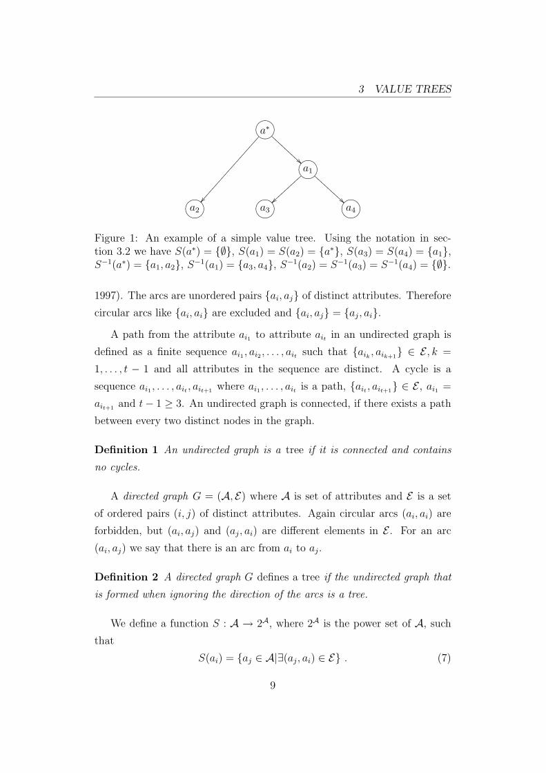
dently of each other. A basic hierarchical value tree with attributes as nodes

is presented in Figure 1. In hierarchical weight elicitation a∗ is often called

7

3 VALUE TREES

the overall goal, which is evaluated through its components related to it ac-

cording to the figure. The attributes lowest in the hierarchy (a2, a3 and a4)

are called twig level attributes.

The value tree in Figure 1 could have been the result of structuring the

portfolio choosing problem of opening new stores in new cities. Then the

attributes could be such that the overall goal is to select the best possible

sites to open stores, a1 the market, a2 the price, a3 the competition and a4

the customers. Obviously the decision could be structured even further by

dividing price into fixed costs and risk or taking stand to the effect on the

whole company like public relations (PR) value, for example.

The hierarchy explicitly accounts the factors influencing the decision,

when deciding the value of a certain property. It should be noted, how-

ever, that the additive value function describes the DM’s preferences if and

only if the attributes are preferentially independent (see Keeney and Raiffa,

1976). Also a value tree should be

(i) Minimal (it contains only relevant attributes)

(ii) Operational (attributes are illustrative and meaningful, i.e. there are

differences between the alternatives in these criteria)

(iii) Complete (all necessary attributes are included)

(iv) Decomposable (attributes can be evaluated individually)

(v) Non-redundant (all attributes appear only once) .

3.2 Mathematical Treatment

This section presents a mathematical framework of value trees suitable for

developing a procedure for obtaining the set Sw. Consider an undirected graph

G = (A, E) consisting of a set of attributes A = {a0, a1, . . . , ap} acting as

nodes and a set of arcs E connecting the attributes (Bertsimas and Tsitsiklis,

8

3 VALUE TREES

GFED@ABCa∗

������

����

����

����

���

AAA

AAAA

AA

GFED@ABCa1

~~||||

||||

|

BBB

BBBB

BB

GFED@ABCa2 GFED@ABCa3 GFED@ABCa4

Figure 1: An example of a simple value tree. Using the notation in sec-tion 3.2 we have S(a∗) = {∅}, S(a1) = S(a2) = {a∗}, S(a3) = S(a4) = {a1},S−1(a∗) = {a1, a2}, S−1(a1) = {a3, a4}, S−1(a2) = S−1(a3) = S−1(a4) = {∅}.

1997). The arcs are unordered pairs {ai, aj} of distinct attributes. Therefore

circular arcs like {ai, ai} are excluded and {ai, aj} = {aj, ai}.

A path from the attribute ai1 to attribute ait in an undirected graph is

defined as a finite sequence ai1 , ai2 , . . . , ait such that {aik , aik+1} ∈ E , k =

1, . . . , t − 1 and all attributes in the sequence are distinct. A cycle is a

sequence ai1 , . . . , ait , ait+1 where ai1 , . . . , ait is a path, {ait , ait+1} ∈ E , ai1 =

ait+1 and t− 1 ≥ 3. An undirected graph is connected, if there exists a path

between every two distinct nodes in the graph.

Definition 1 An undirected graph is a tree if it is connected and contains

no cycles.

A directed graph G = (A, E) where A is set of attributes and E is a set

of ordered pairs (i, j) of distinct attributes. Again circular arcs (ai, ai) are

forbidden, but (ai, aj) and (aj, ai) are different elements in E . For an arc

(ai, aj) we say that there is an arc from ai to aj.

Definition 2 A directed graph G defines a tree if the undirected graph that

is formed when ignoring the direction of the arcs is a tree.

We define a function S : A → 2A, where 2A is the power set of A, such

that

S(ai) = {aj ∈ A|∃(aj, ai) ∈ E} . (7)

9

3 VALUE TREES

The set S(ai) includes the attributes having an arc from them to the node

ai. The inverse function S−1 : A → 2A is defined as

S−1(ai) = {aj ∈ A|ai ∈ S(aj)} . (8)

The set S−1(ai) includes all attributes which ai has an arc going to. The

functions S and S−1 defines the overall goal and twig level attributes.

Definition 3 An attribute ai is an overall goal if S(ai) = {∅}.

Definition 4 An attribute ai is a twig level attribute if S−1(ai) = {∅}.

Definition 5 A directed graph G = (A, E) is a hierarchical value tree if

(i) G defines a tree,

(ii) G has exactly one overall goal a∗ and

(iii) |S(ai)| = 1 ∀ai ∈ A, where the number of elements in a set X is denoted

by |X| and |{∅}| = 1.

Assume that G is a hierarchical value tree with the attributes A = {a∗}∪{ai|i = 1, . . . p}, a∗ is the overall goal and the set At := {ai ∈ A|S−1(ai) =

∅} contains all the twig level attributes. The twig level attribute function

L : A → 2At is defined recursively as

L(ai) =

{ai} ai ∈ At⋃

aj∈S−1(ai)

L(aj), otherwise (9)

In other words, the set L(ai) is the set of twig level attributes that are below

ai in the hierarchy. It is also clear by construction, that L(a∗) = At.

Each attribute ai is assigned a weight wi ∈ [0, 1] such that for twig level

attributes ∑ai∈At

wi = 1, wi ≥ 0

10

3 VALUE TREES

and for all other attributes

wi =∑

aj∈L(ai)

wj . (10)

Thus, the weights of twig level attributes {wi|ai ∈ At} are sufficient to define

all the weights.

The DM’s preferences are modeled through linear constraints on the

weights. For instance, assume that attribute a1 is more important than

a2, implying that a change from the worst to the best performance level in

a1 has more influence on the overall value than the corresponding change in

a2. Then the weight w1 must be larger than w2. Any such statement on

attributes A′ ∈ A can be expressed in the form∑ai∈A′

ciwi ≤ b, A′ ⊆ A . (11)

These restrictions can be presented through weighted sums of twig level at-

tribute weights. By substituting (10) to (11) we get∑ai∈A′

ci

∑aj∈L(ai)

wj ≤ b ⇐⇒∑

ak∈At

ckwk ≤ b

ck =∑j∈Jk

cj, Jk = {j ∈ N|aj ∈ A′ ∧ ak ∈ L(aj)} .(12)

Thus any preference statement at any level of the value tree can be expressed

with constraints on the twig level attributes. These types of restrictions are

supported by RPM, so we have established a new method for giving prefer-

ence information compatible with RPM. The restrictions can be presented

in matrix form Aww ≤ bw, giving us the information set

Sw = {w ∈ S0w|Aww ≤ bw} ,

which is compatible with (5). In fact, we have reduced the tree structure

to a one level tree which means taking a weighted average of the twig level

attribute scores. If we want to ensure that hierarchy is respected, i.e. only

11

4 SOFTWARE IMPLEMENTATION

attributes with the same attribute on the next higher level of the hierarchy

are compared, we demand that A′ ⊆ S−1(ai) for some ai ∈ A.

Let us continue our earlier example involving Figure 1 by giving ordinal

preference information about the attributes. Assume that when deciding the

overall goal, price (a2) is more important than the market (a1) and when

evaluating the market, customers (a4) are more important than competition

(a3). To have compatible information, the associated weights wi would have

to fulfil the constraintsw2 ≥ w1

w3 ≥ w4

.

Expressed with twig level attribute weights using (12) this would correspond

tow2 ≥ w3 + w4

w3 ≥ w4

.

4 Software Implementation

The value tree framework presented in this study is implemented in a decision

support software RPM-Decisions. The software is a Javatm-program with a

graphical user interface (GUI). Incomplete information on weights can be

given by defining the weight constraints (i.e. the elements of the matrix

Aw and the vector bw) using spreadsheets. However, it is quite hard to

produce the elements resulting from transforming statements in a value tree

without computational support. Therefore a preference elicitation tool was

implemented, which automatically generates these constraints as the user

defines her preferences.

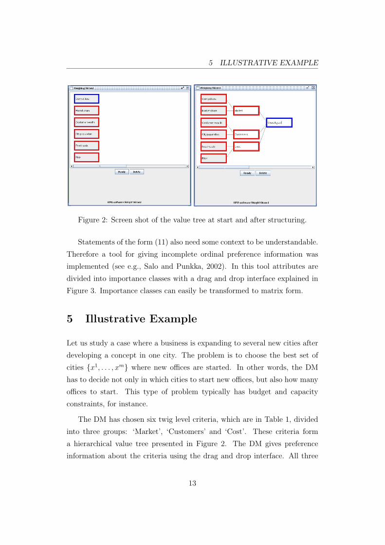
The value tree tool includes an interface for building the tree, illustrated

in Figure 2. Each attribute in the tree, except the twig level attributes, can

be assigned preference information about the attributes one level lower in the

hierarchy. By double-clicking on an attribute statements of the form (11) can

be given.

12

5 ILLUSTRATIVE EXAMPLE

Figure 2: Screen shot of the value tree at start and after structuring.

Statements of the form (11) also need some context to be understandable.

Therefore a tool for giving incomplete ordinal preference information was

implemented (see e.g., Salo and Punkka, 2002). In this tool attributes are

divided into importance classes with a drag and drop interface explained in

Figure 3. Importance classes can easily be transformed to matrix form.

5 Illustrative Example

Let us study a case where a business is expanding to several new cities after

developing a concept in one city. The problem is to choose the best set of

cities {x1, . . . , xm} where new offices are started. In other words, the DM

has to decide not only in which cities to start new offices, but also how many

offices to start. This type of problem typically has budget and capacity

constraints, for instance.

The DM has chosen six twig level criteria, which are in Table 1, divided

into three groups: ‘Market’, ‘Customers’ and ‘Cost’. These criteria form

a hierarchical value tree presented in Figure 2. The DM gives preference

information about the criteria using the drag and drop interface. All three

13

5 ILLUSTRATIVE EXAMPLE

a1

_ _ _ _ _ _ _ _ _ _ _ _����������������

����������������_ _ _ _ _ _ _ _ _ _ _ _

1b76540123``

a1

765401231a

22

a2 a3

a4

a5

a1

_ _ _ _ _ _ _ _ _ _ _ _����������������

����������������_ _ _ _ _ _ _ _ _ _ _ _

a2 a3

/.-,()*+2rra4 a3

a5

a1

_ _ _ _ _ _ _ _ _ _ _ _����������������

����������������_ _ _ _ _ _ _ _ _ _ _ _

a2

a5 a4 a3

a5

765401233a

22

3b76540123~~

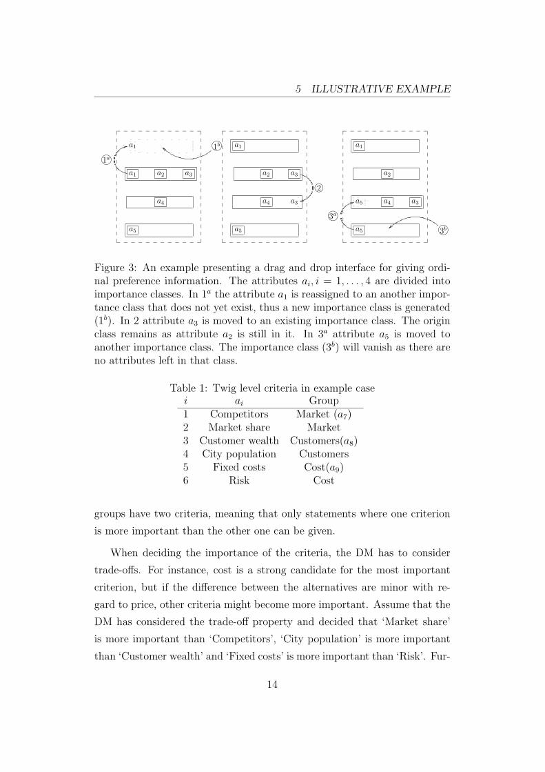
Figure 3: An example presenting a drag and drop interface for giving ordi-nal preference information. The attributes ai, i = 1, . . . , 4 are divided intoimportance classes. In 1a the attribute a1 is reassigned to an another impor-tance class that does not yet exist, thus a new importance class is generated(1b). In 2 attribute a3 is moved to an existing importance class. The originclass remains as attribute a2 is still in it. In 3a attribute a5 is moved toanother importance class. The importance class (3b) will vanish as there areno attributes left in that class.

Table 1: Twig level criteria in example casei ai Group1 Competitors Market (a7)2 Market share Market3 Customer wealth Customers(a8)4 City population Customers5 Fixed costs Cost(a9)6 Risk Cost

groups have two criteria, meaning that only statements where one criterion

is more important than the other one can be given.

When deciding the importance of the criteria, the DM has to consider

trade-offs. For instance, cost is a strong candidate for the most important

criterion, but if the difference between the alternatives are minor with re-

gard to price, other criteria might become more important. Assume that the

DM has considered the trade-off property and decided that ‘Market share’

is more important than ‘Competitors’, ‘City population’ is more important

than ‘Customer wealth’ and ‘Fixed costs’ is more important than ‘Risk’. Fur-

14

5 ILLUSTRATIVE EXAMPLE

thermore the DM assesses ‘Market’ as the most important criterion under

the overall goal but cannot decide which one of the remaining criteria ‘Cus-

tomers’ and ‘Cost’ is more important. This information corresponds to the

linear constraintsw2 ≥ w1

w4 ≥ w3

w5 ≥ w6

w7 ≥ w8

w7 ≥ w9 .

Using equation (10), we get additionally the linear equality constraints

w7 = w1 + w2

w8 = w3 + w4

w9 = w5 + w6 .

In terms of twig level criteria weights, these constraints are equal to

Aww =

1 −1 0 0 0 00 0 1 −1 0 00 0 0 0 −1 1−1 −1 1 1 0 0−1 −1 0 0 1 1

w1

w2

w3

w4

w5

w6

≤

000000

= bw .

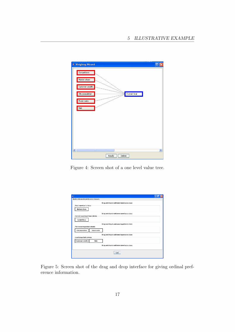
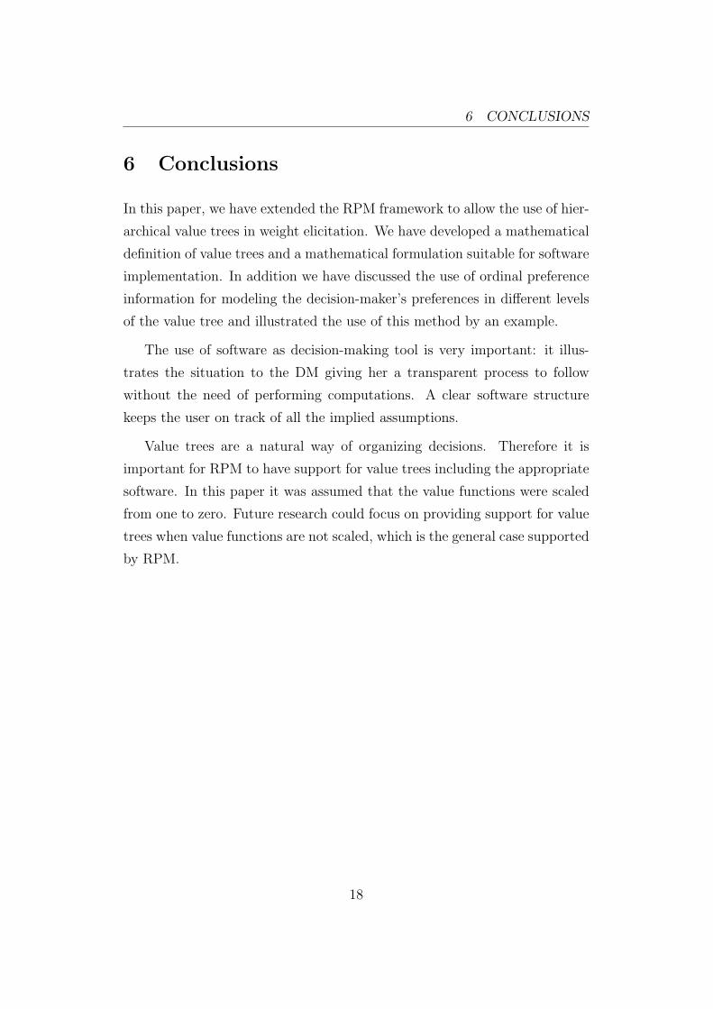
For comparison, assume that the DM would not want to structure her

decision into a multilevel tree, but would like to compare the twig level

attributes directly (see Figure 4). The information she gives would be such

that ‘Market share’ is the most important, ‘Competitors’ second most impor-

tant, ‘City population’ and ‘Fixed costs’ third most important and ‘Customer

wealth’ and ‘Risk’ the least important (see Figure 5). This would correspond

15

5 ILLUSTRATIVE EXAMPLE

to the set of constraints

Aww =

−1 1 0 0 0 00 −1 0 1 0 00 −1 0 0 1 00 0 1 −1 0 00 0 0 −1 0 10 0 1 0 −1 00 0 0 0 −1 1

w1

w2

w3

w4

w5

w6

≤

0000000

= bw .

16

5 ILLUSTRATIVE EXAMPLE

Figure 4: Screen shot of a one level value tree.

Figure 5: Screen shot of the drag and drop interface for giving ordinal pref-erence information.

17

6 CONCLUSIONS

6 Conclusions

In this paper, we have extended the RPM framework to allow the use of hier-

archical value trees in weight elicitation. We have developed a mathematical

definition of value trees and a mathematical formulation suitable for software

implementation. In addition we have discussed the use of ordinal preference

information for modeling the decision-maker’s preferences in different levels

of the value tree and illustrated the use of this method by an example.

The use of software as decision-making tool is very important: it illus-

trates the situation to the DM giving her a transparent process to follow

without the need of performing computations. A clear software structure

keeps the user on track of all the implied assumptions.

Value trees are a natural way of organizing decisions. Therefore it is

important for RPM to have support for value trees including the appropriate

software. In this paper it was assumed that the value functions were scaled

from one to zero. Future research could focus on providing support for value

trees when value functions are not scaled, which is the general case supported

by RPM.

18

REFERENCES

References

[1] Belton, V. and Stewart, T.J. (2001). Multiple criteria decision analysis:

An integrated approach. Kluwer Academic Publishers, Boston.

[2] Bertsimas, D. and Tsitsiklis J. (1997). Introduction to Linear Optimiza-

tion. Athena Scientific, Belmont.

[3] Golabi, K. (1987). Selecting a Group of Dissimilar Projects for Funding.

IEEE Transactions on Engineering Management, vol. 34, pp. 138-145.

[4] Golabi, K., Kirkwood, W.C. and Sicherman, A. (1981). Selecting a port-

folio of solar energy projects using multiattribute preference theory Man-

agement Science, vol. 27, pp. 174-189.

[5] Keeney, R.L. and Raiffa, H. (1976). Decisions with multiple objectives:

Preferences and value tradeoffs. John Wiley & Sons, New York.

[6] Kim, S.H. and Ahn, B.S. (1999) Interactive group decision making pro-

cedure under incomplete information. European Journal of Operational

Research, vol. 116, pp. 498-507.

[7] Kleinmuntz, C.E., Kleinmuntz, D.N., (1999). Strategic Approaches for

Allocating Capital in Healthcare Organizations, Healthcare Financial

Management, Vol. 53, pp. 52-58.

[8] Liesio, J., Mild, P., Salo, A. (2004) Preference programming for robust

portfolio modeling and project selection. European Journal of Opera-

tional Research (to appear)

[9] Liesio, J., Mild, P., Salo, A. (2006). Robust Portfolio Modeling with

Project Interdependencies and Balance Constraints, Helsinki University

of Technology. European Journal of Operational Research (to appear).

[10] Punkka, A. (2002). Use of RICH in Multi-level Value Trees. Independent

Research Project in Applied Mathematics. Systems Analysis Laboratory,

19

REFERENCES

Helsinki University of Technology. Available at

http://www.sal.tkk.fi/Opinnot/Mat-2.108/pdf-files/epun02b.pdf.

[11] Rios Insua, D. and French, S. (1991). A framework for sensitivity anal-

ysis in discrete multi-objective decision making. European Journal of

Operational Research, vol. 54, pp. 176-190.

[12] Saaty, T.L. (1980). The Analytical Hierarchy Process. McGraw-Hill,

New York.

[13] Salo, A. and Hamalainen, R.P. (2004). Preference programming. Sys-

tems Analysis Laboratory, Helsinki University of Technology. Available

at http://www.sal.hut.fi/Publications/pdf-files/msal03b.pdf.

[14] Salo, A. and Punkka, A. (2005) Rank Inclusion in Criteria Hierarchies,

European Journal of Operational Research, Vol. 163, pp. 338-356.

20