Embed Size (px)
DESCRIPTION
vol smile
Citation preview

Heterogeneous Beliefs and The Option-implied Volatility Smile
Geoffrey C. Friesen University of Nebraska-Lincoln
[email protected] (402) 472-2334
Yi Zhang* Prairie View A&M University
[email protected] (936) 261-9219
Thomas S. Zorn University of Nebraska-Lincoln
[email protected] (402) 472-6049
*Corresponding author

1
Heterogeneous Beliefs and The Option-implied Volatility Smile
Abstract
Recent studies suggest that differences in investor beliefs may help explain the
volatility smile. We examine the cross-sectional relation between the volatility smile and
heterogeneous beliefs using data on stock options traded on the CBOE from 2003 to
2005. Using several widely used proxies for heterogeneous beliefs, including the
dispersion in financial analysts’ earnings forecasts, option open interest and stock trading
volume, we find that stocks with greater belief differences have more pronounced
volatility smiles. We further use factor analysis to identify a latent variable for
heterogeneous beliefs, and find a strong relationship between the latent variable and the
volatility smile.

2
Introduction
Equilibrium asset prices reflect investors’ beliefs about asset values. Many
financial models assume these beliefs are homogeneous. Even a casual acquaintance with
investment advisors and commentators suggests that belief homogeneity is a fairly heroic
assumption. It is possible, however, that belief differences may wash out and in many
applications not matter all that much. The importance of belief differences in explaining
asset prices is therefore an empirical issue.1
Several recent papers have suggested that the option-implied volatility smile may
be related to investors’ belief differences.
2 Shefrin (2001) demonstrates that investor
sentiment affects the pricing kernel in such a way that belief differences can lead to a
volatility smile. Similarly, Ziegler (2003) shows that belief differences can impact
equilibrium state-price densities, and thus may help explain the volatility smile. Buraschi
and Jiltsov (2006) develop an option pricing and volume model in which agents have
heterogeneous beliefs on expected returns and face model uncertainty. They show that
heterogeneous beliefs about the dividend growth rate affect option prices and volume and
produce a volatility smile. In their model, optimistic investors demand out-of-the-money
calls while pessimistic investors demand out-of-the-money puts.3
This study examines the empirical relationship between heterogeneous beliefs and
the option-implied volatility smile using cross-sectional data. While previous studies
1 Belief differences may arise due to information differences or differing interpretations of information and have the potential to dramatically impact asset prices and trading dynamics. Harris and Raviv (1993), Detemple and Murphy (1994), Basak (2000), Shefrin (2001) and Basak (2005) all suggest that belief differences affect asset prices or trading. 2 The option-implied volatility is the volatility level at which the Black-Scholes option price equals the option’s observed market price. The documented U-shaped variation in the implied volatility across different strike prices is called the volatility smile. 3 Li (2007) also develops an option pricing model in which investors have heterogeneous beliefs about the dividend growth rate, have different time preferences. In that model the implied volatility smile depends on belief differences, time preferences and relative wealth of investors.
3
have focused on the time-series analysis of index options (Shefrin, 1999; Buraschi and
Jiltsov, 2006), we examine individual stock options traded on the Chicago Board Options
Exchange (CBOE) from 2003 to 2005. Looking at individual options allows us to test for
cross-sectional relationships between belief differences and smile slope. If heterogeneous
investor beliefs affect option prices then the volatility smile will be more pronounced for
those assets with greater belief heterogeneity. Since beliefs are not directly observable,
we draw upon the existing empirical literature to examine six different proxies for belief
differences.
We find that stocks with greater dispersion in financial analysts’ earnings
forecasts, higher trading volume and a greater amount of open interest in out-of-the-
money options have more pronounced volatility smiles. The volatility smile is also more
pronounced for small stocks and growth stocks (low earnings-to-price ratio) relative to
large stocks and income stocks (high earnings-to-price ratio), respectively. In addition,
stocks with high book-to-market ratios have more pronounced volatility smiles than
stocks with low book-to-market ratios. These results lend support to the argument that the
volatility smile is related to belief differences among investors.4
Each of the belief proxies utilized above are at best noisy measures of investor
beliefs. The second contribution of this study is to use factor analysis to identify a latent
investor belief variable. If the observable proxy variables for heterogeneous beliefs
4 The dispersion in financial analysts’ earnings forecasts has been widely used in literature to proxy for the dispersion of opinions among investors (e.g. Diether et al., 2002). Stock trading volume is another widely used proxy for heterogeneous beliefs because more divergent beliefs among investors tend to induce more trading volume (e.g. Harris and Raviv, 1993). In addition, option open interest is used to proxy for heterogeneous beliefs as the put/call open interest ratio is widely used in behavioral finance as a measure of investor sentiment (e.g. Dennis and Mayhew, 2002). Also, differences in beliefs among investors tend to be greater for small firms than for large firms since small firms have less information available for the public. Growth stocks (low earnings-to-price ratio) tend to induce more divergent estimations on the dividend growth rate than income stocks (high earnings-to-price ratio). In addition, Diether et al. (2002) and others find that differences in beliefs tend to be greater for stocks with a high book-to-market ratio than stocks with a low book-to-market ratio.

4
capture the unobservable differences in beliefs, a latent variable should be identifiable
using factor analysis. We use the previously mentioned proxies for heterogeneous beliefs
to conduct a factor analysis, which produces two latent factors. The first factor is highly
loaded with firm size, open interest and stock trading volume. We suggest that the
loadings on this factor are consistent with the presence of an underlying size factor. The
second factor is highly loaded with the dispersion in financial analysts’ earnings forecasts
and the earnings-to-price ratio, and appears to reflect heterogeneity in investor beliefs.
We then use the latent factor for belief differences, which is a cleaner measure
than the individual proxies, to examine the relationship between belief differences and
the volatility smile. We find a strong relationship between the volatility smile and the
latent factor. Results using the latent factor are more significant than those produced
using proxy variables.
This paper is organized as follows: Section I describes related literature regarding
the volatility smile. Section II develops hypotheses on the relation between
heterogeneous beliefs and the volatility smile. Section III describes data and empirical
methodology. Section IV presents empirical results and Section V discusses the
robustness of results. Section VI concludes this study.
I. Related Literature
There are various explanations for the volatility smile, which refers to the
observed tendency of option-implied volatility to vary across strike prices. Some
explanations relate to violations of the assumptions of the Black-Scholes model (e.g.
violations of lognormally distributed returns or constant volatility). For instance, Hull
(1993) points out that the volatility smile may be a consequence of empirical violations of
the assumption of the normality of the log return. In addition, Bakshi et al., 2003 show

5
that leptokurtic returns will cause the Black-Scholes model to misprice out-of-the-money
(OTM) or in-the-money (ITM) options. Hull and White (1988) and Heston (1993)
suggest that the volatility smile reflects stochastic volatility. If the volatility is stochastic
and innovations to the volatility are negatively (positively) correlated with underlying
asset returns, a stochastic volatility model can generate the observed downward (upward)
slope of the implied volatility. Pena et al. (1999) show that transaction costs also affect
the curvature of the volatility smile.
An alternative explanation for the volatility smile is the leverage argument. As a
company’s equity value declines, the company’s leverage increases and thus the equity
becomes more risky and its volatility increases. This argument explains the inverse
relationship between volatility and prices. Toft and Prucyk (1997) find more highly
levered firms have steeper smiles. Other studies suggest that firm-specific factors are
more important than the variation in systematic factors in explaining the smiles of
individual stock options. For example, Dennis and Mayhew (2002) find the volatility
smile of stock options is affected by liquidity and market risk measured by beta and size.
Another direction of research relates the volatility smile to market participants.
Bollen and Whaley (2004) find net buying pressure determines the shape of the volatility
smile, which they attribute to limits to arbitrage. They find that the shape of the implied
volatility function of individual stock options are directly related to net buying pressure
of call option demand. Alternatively, several studies such as Shefrin (2001), Ziegler
(2003), Buraschi and Jiltsov (2006) and Li (2007) relate the volatility smile to
heterogeneous beliefs of investors. These studies show that heterogeneous beliefs impact
the value of options and thus can explain the volatility smile.
Shefrin (1999) shows the volatility smile on S&P 500 index options is one
manifestation stemming from heterogeneous beliefs. Optimistic investors drive up the

6
price of OTM calls while pessimistic investors drive up the price of OTM puts. The
greater the divergence of opinions, the stronger the volatility smile. Shefrin (2001)
shows that investor sentiment affects the pricing kernel so that the log stochastic discount
factor (SDF) is U-shaped rather than monotonically decreasing, as assumed in standard
asset pricing models. The U-shape in the log-SDF gives rise to the volatility smile in
option prices. Ziegler (2003) also demonstrates that heterogeneous beliefs can have a
dramatic impact on equilibrium state-price densities, thus providing an explanation for
the volatility smile.
Buraschi and Jiltsov (2006) study the option pricing and trading volume for an
economy in which agents face model uncertainty and have different beliefs on expected
returns. When agents have different posterior beliefs of the dividend growth rate by
updating their initial beliefs using all available information, they select different optimal
portfolios and trading occurs. More pessimistic agents demand OTM put options while
more optimistic agents demand OTM call options from the pessimists. Therefore
differences in beliefs drive the trading volume of options. Furthermore, differences in
beliefs on the dividend growth rate generate endogenous stochastic volatility of the
underlying stock price and thus cause the option-implied volatility smile: an OTM put is
more expensive than an OTM call. Using S&P 500 index options data and an Index of
Dispersion in Beliefs constructed from survey data, they demonstrate that greater
dispersion in beliefs results in greater open interest and a steeper volatility smile.
Li (2007) develops a model of option prices in an economy in which investors
have different time preferences and heterogeneous beliefs about the dividend growth rate.
The pattern of the implied volatility depends on the beliefs, time preferences and relative
wealth of investors. When pessimistic investors hold a relatively large portion of total

7
wealth the implied volatility exhibits a “skew”; when optimistic investors hold a
relatively large portion of total wealth the implied volatility exhibits a “smile”.
II. Hypothesis Development
If heterogeneous beliefs affect the volatility smile, as the models in the previous
section suggest, then greater belief differences will result in more pronounced volatility
smiles. Our study seeks to examine empirically the relationship between belief
differences and the volatility smile. While the theoretical models provide a motivation for
our empirical work, our empirical findings do not depend on the validity of specific
assumptions from particular models.
The determining characteristic of the volatility smile is that the implied volatility
for out-of-the-money (OTM) individual stock options (both OTM puts and OTM calls) is
greater than the implied volatility of at-the-money (ATM) options. When the implied
volatility (vertical axis) is plotted against the strike price (horizontal axis), the put slope is
therefore negative and the call slope is positive.5
Many empirical studies of the dispersion of opinions, such as Diether et al. (2002)
and Baik and Park (2003), find that the dispersion of opinions among investors tends to
be greater for small firms than large firms. Because financial analysts and the financial
press tend to follow large firms (for the obvious reason that they affect more investors
and have greater relative importance to the economy) investors may have more divergent
beliefs about the value of small firms. Belief differences, to the extent that they are
When we refer to a more “pronounced
smile”, we are describing absolute slope: “more pronounced” is defined as a more
negative put slope and a more positive call slope.
5 More details on the measure of the put slope and the call slope are discussed in Section III.

8
reflected in options, imply that the volatility smile is expected to be more pronounced for
options on small stocks than large stocks. Hence the first hypothesis:
Hypothesis I: Small stocks have more pronounced volatility smiles than large
stocks. Equivalently, firm size should be positively related to the put slope (which
is negative) and negatively related to the call slope (which is positive).
In the equity market, shares of companies that are growing at an above average
rate relative to their industry are commonly called growth stocks. Growth stocks
normally pay smaller dividends, as the company prefers to reinvest retained earnings in
capital projects. In contrast, income stocks tend to pay out larger dividends. Growth
stocks tend to induce a greater amount of heterogeneity in investor beliefs about
dividend growth rates compared to income stocks. One common method to distinguish
growth stocks and income stocks is the earnings-to-price ratio: growth stocks have low
earnings-to-price ratios while income stocks have high earnings-to-price ratios. Baik and
Park (2003) find stocks with lower earnings-to-price ratios have more dispersion in
financial analysts’ earnings forecasts, consistent with the idea that growth stocks have
greater belief heterogeneity. Thus the second hypothesis:
Hypothesis II: Growth stocks have more pronounced volatility smiles than income
stocks. Equivalently, the earnings-to-price ratio should be positively related to
the put slope and negatively related to the call slope.
In addition, Diether et al. (2002), Baik and Park (2003) and Doukas et al. (2004)
find that stocks with high book-to-market ratios have larger dispersion in financial
analysts’ earnings forecasts than stocks with low book-to-market ratios. They use this
finding to suggest that the dispersion in financial analysts’ earnings forecasts is a proxy

9
for differences in investor opinions about a stock. Likewise, we assume that stocks with
high book-to-market ratios have greater heterogeneity in investor beliefs. The third
hypothesis is therefore:
Hypothesis III: Stocks with higher book-to-market ratios have more pronounced
volatility smiles than stocks with lower book-to-market ratios. Equivalently, the
book-to-market ratio should be negatively related to the put slope and positively
related to the call slope.
Furthermore, if the volatility smile is related to heterogeneous beliefs, it is
expected to be correlated with widely used proxies for heterogeneous beliefs. The
dispersion in financial analysts’ earnings forecasts is used to proxy for heterogeneous
beliefs by Diether et al. (2002), Doukas et al. (2004) and others. Goetzmann and Massa
(2003) show that dispersion of opinion among investors is correlated with dispersion of
opinion among financial analysts. Therefore, stocks with a greater dispersion in financial
analysts’ earnings forecasts are expected to have more pronounced volatility smiles.
Hence the fourth hypothesis:
Hypothesis IV: Stocks with a greater dispersion in financial analysts’ earnings
forecasts have more pronounced volatility smiles than stocks with less dispersion
in financial analysts’ earnings forecasts. Equivalently, the dispersion in financial
analysts’ earnings forecasts should be negatively related to the put slope and
positively related to the call slope.
Another proxy for heterogeneous beliefs is the open interest on options. The
put/call open interest ratio is commonly believed to be a measure of investor sentiment:
more put open interest indicates pessimism while more call open interest indicates

10
optimism. Optimistic investors demand OTM calls because they provide upside potential
while pessimistic investors demand OTM puts because they provide downside protection.
Buraschi and Jiltsov (2006) show that more heterogeneity in investor beliefs produces
greater open interest. Dennis and Mayhew (2002) use open interest to proxy for belief
differences. In addition, stock trading volume is suggested to be another proxy for
heterogeneous beliefs by Harris and Raviv (1993), Kandel and Pearson (1995), Odean
(1998) and Hong and Stein (2003). Since belief differences induce trades, stocks with
more divergent beliefs among investors tend to induce greater trading volume. Therefore
both option open interest and stock trading volume are expected to be correlated with the
volatility smile. This leads to the following two hypotheses:
Hypothesis V: Stocks with more OTM option open interest have more pronounced
volatility smiles. Equivalently, the put slope should be negatively related to OTM
put option open interest while the call slope should be positively related to OTM
call option open interest.
Hypothesis VI: Stocks with more trading volume have more pronounced volatility
smiles. Equivalently, the stock trading volume should be negatively related to the
put slope and positively related to the call slope.
If the above proxy variables are all related to heterogeneous beliefs, the
underlying belief differences should be identifiable using factor analysis. The factor
model in matrix form is assumed to be:
η+Λ= fz (1)

11
where z is the vector of standardized proxies, f is the factor vector with zero means and
one variances; Λ is the matrix of factor loading and η is independent of the factor vector.
The factor model implies that
Ψ+Λ′Λ=+Λ′Λ==Σ )()( ηCovzCov (2)
The goal of factor analysis is to find Λ and Ψ that satisfy the factor analysis equations
(2). If a latent factor for heterogeneous beliefs is successfully identified, we can estimate
the factor as the linear combination of proxy variables using factor score coefficients:
zSf *= (3)
where S is the factor score coefficient matrix. Our last hypothesis is:
Hypothesis VII: The latent factor for heterogeneous beliefs should be negatively
related to the put slope and positively related to the call slope.
III. Data and Methodology
A. Data and Variable Construction
This study uses a dataset on options traded on the Chicago Board Options
Exchange (CBOE) from 2003 to 2005 provided by deltaneutral.com. The option data
contain trading prices, bid-ask quotes, volume, open interest, implied volatility and the
underlying security price. The implied volatility is calculated using the mid-point of the
bid and ask prices and inverting the Black-Scholes model using the bisection method.6
6 Individual stock options are American options with a potential for early exercise. Using the Black-Scholes model to calculate the implied volatility does not account for the possibility of early exercise. However, Bakshi et al. (2003) also use the Black-Scholes to compute the implied volatility to adhere to convention since they find the difference between the American option implied volatility and its Black-Scholes counterpart is negligible. Also errors in using the Black-Scholes model to back out the implied volatility are less important for this study because the analysis relies on the slope of the volatility smile (i.e. the relative magnitude of the implied volatility of OTM options compared to ATM options) rather than the level of the implied volatility.
To
be consistent with the existing literature, any option that violates basic arbitrage bounds is

12
deleted. Options with zero open interest are also deleted. Since ITM options are less
liquid than ATM or OTM options, the small volume of ITM options makes the quoted
prices noisy. As optimistic investors demand OTM call options while pessimistic
investors demand OTM put options, investor beliefs can be sufficiently reflected in OTM
options. Therefore only OTM options are considered in this study.7
Unlike index options which exhibit monotonically decreasing implied volatilities
with strike prices, implied volatilities of most stock options exhibit a “smile” shape. We
follow Bollen and Whaley (2004) and consider separately the smile slopes of OTM puts
and OTM calls.
Only stocks which
have both OTM puts and OTM calls are selected. Since most transactions are
concentrated in the nearest expiration contracts, we use only options with the shortest
time to maturity. Following Whaley (1993), options with maturities less than seven days
are eliminated. Therefore the sample is restricted to options with maturities between 7
and 30 days.
8
• ATM options (0.95<=X/S<=1.05);
Using their moneyness, defined as the ratio of the strike price (X) to
stock market price (S), options are categorized as follows:
• OTM calls (X/S>1.05);
• OTM puts (X/S<0.95).
The smile slope for OTM options is computed as the difference between the
implied volatility of OTM options (IVOTM) and the implied volatility of ATM options
7 We compare the implied volatility of ITM options with OTM options and find they are very close. Buraschi and Jiltsov (2006) and Bakshi et al. (2003) both only use OTM options. 8 Buraschi and Jiltsov (2006) measures the smile as the difference of the implied volatility of OTM puts and OTM calls because the implied volatilities of index options decrease monotonically across strike prices. However, this methodology will fail to capture the variation of the implied volatility of individual stock options if they exhibit a “smile”.

13
(IVATM) on the same underlying stock with the same expiration, divided by the difference
between the moneyness of OTM options and the moneyness of ATM options:
ATMOTM
ATMOTMi MoneynessMoneyness
IVIVSLOPE
i
i
−
−= (4)
where i=call or put.
To avoid differences in smile slopes driven by differences in stock price levels,
moneyness is employed because it is comparable across stocks. If the implied volatility
across the moneyness exhibits a “smile” shape, the put slope is negative and the call slope
is positive. Section V examines the robustness of our results to alternative measures of
smile slope.
Each day the implied volatility and the moneyness of options are averaged over
all strike prices in each moneyness category, and then the put slope and the call slope are
calculated. To test whether the volatility smile is related to heterogeneous beliefs at a
cross-sectional level, we regress the smile slope on various proxies for heterogeneous
beliefs described in Section II. In addition, we include several other control variables.
Pena et al. (1999) find that transaction costs seem to be a key determinant of the
curvature of the volatility smile. We follow Pena et al. (1999) and use the bid-ask spread
of the closing prices for OTM options as a proxy for transaction costs.9
Time-to-expiration and market uncertainty are also included as control variables.
Time-to-expiration is measured as the number of calendar days between the trade date
and the expiration date. Market uncertainty is measured each month as the standard
The bid-ask
spread reflects the market-making costs and adverse selection risks faced by investors in
options markets. Options with high bid-ask spreads are expected to have steeper smiles
than options with low bid-ask spreads.
9 Pena et al. (1999) use 45-minute interval.

14
deviation of daily returns of value-weighted index including distributions. Return data are
obtained from the Center for Research in Securities Prices (CRSP). Option volume is
used as a control variable to proxy for liquidity. Option volume is summed over all
options in each moneyness category. In addition, each firm’s market risk and
idiosyncratic risk are also used as control variables. These are calculated each month by
regressing daily stock returns on the daily returns of value-weighted index including
distributions. Market risk is measured as beta and the idiosyncratic risk is measured as
the standard deviation of residuals from the market model regression.
Firm-specific variables are constructed each month using the data from the CRSP
and the Compustat Industrial Quarterly File. Firm size is measured as the natural
logarithm of market capitalization (stock price multiplied by the number of outstanding
shares) as of the last trading day of the previous month. The earnings-to-price ratio is
measured as the quarterly earnings (Data 27) divided by the stock price as of the last day
of the previous month.10
Following Diether et al. (2002), the dispersion in financial analysts’ earnings
forecasts is measured as the standard deviation of forecasts for quarterly earnings scaled
by the absolute value of the mean earnings forecast. The data on financial analysts’
earnings forecasts are taken from the Institutional Brokers Estimate System (I/B/E/S)
The book-to-market ratio is measured as the book value of
common equity (Data 59) divided by the market capitalization as of the last day of the
previous month. Leverage is defined as the debt-to-equity ratio, computed as the long
term debt (Data 51) divided by the market capitalization as of the last day of the previous
month. For robustness checks, the above firm specific variables are also computed using
daily stock prices rather than prices as of the last day of the previous month. The results
based on daily stock prices are discussed in Section V.
10 We ignore observations with a negative earnings-to-price ratio.

15
summary history dataset. Only the most recent statistical summary is adopted for a given
month. To make sure the forecast is current, only the forecast period of one quarter
(FPI=6) is selected. Firms with a zero mean forecast or without a standard deviation due
to only one forecast available are excluded.
B. Factor Analysis Methodology
To conduct the factor analysis, proxy variables are measured at the monthly
frequency. OPEN INTEREST is the average daily total open interest of both OTM puts
and OTM calls. Since the units across six proxies vary by several orders of magnitude,
using raw data leads to over-weighting some proxies simply because their scale makes
them seem much more variable than other proxies. Therefore according to the
convention, the Spearman correlation matrix is applied, which is similar to standardizing
the data by subtracting the mean and then dividing by standard deviation.
We adopt two common methods for solving factor analysis equations: the
maximum likelihood method and the principal factor method.11
IV. Empirical Results
We follow the common
practice of rotating factors to facilitate their interpretation, which normalizes as many of
the factor loadings as possible close to zero. We adopt the most widely used orthogonal
rotation method: the Varimax orthogonal rotation method proposed by Kaiser (1958),
which ensures that factors are uncorrelated with each other.
A. Results Based on Proxy Variables
11 The algorithms of the procedure can be found in the appendix. A factor analysis initially requires suitable estimates of the communalities. The communality estimate for a variable is the proportion of the variance of each variable that is explained by the common factors. We choose one common approach to set the prior communality estimate for each variable to its squared multiple correlation of each variable with all remaining variables.

16
Table I presents summary statistics for option-implied volatilities and smile
slopes. The sample includes options on 865 stocks. The mean (median) implied volatility
of OTM puts is 85% (73%) and the mean (median) implied volatility of OTM calls is
66% (57%). Both are higher than the mean (median) implied volatility of ATM options
46% (43%). The average put slope is -1.59, steeper than the average call slope 0.68. As
argued in Buraschi and Jiltsov (2006), because the marginal utility is higher (lower) in
bad (good) states of the world, the cost of an OTM put is higher than that of an OTM call,
thus the implied volatility of an OTM put is higher than that of an OTM call.
Consistent with the findings of Bollen and Whaley (2004), about 82% of our
sample exhibit a “smile” shape. The average implied volatility of the smile sample
(117,836 observations) is plotted across the moneyness in Figure 1a. The put slope is
negative (-1.72) and steeper than the call slope (0.89). About 18% of the sample (25,574
observations) exhibits monotonically decreasing implied volatilities with strike prices,
which we refer to as the volatility skew (see Figure 1b). The mean put slope and the mean
call slope are negative: -1.16 and -0.25 respectively, but the put slope is much steeper
than the call slope. A small number of observations in our sample exhibit shapes not
characterized as a smile or a skew, and these observations are omitted from the analysis.
[Insert Table I here]
[Insert Figure 1 here]
Figure 2 shows the term structure of the implied volatility – the variation of the
implied volatility with the maturity of the option. The implied volatilities of OTM puts
and OTM calls increase as options become closer to expiration. The implied volatilities
of short-dated ATM options in the smile sample are nearly constant across time-to-
expiration as shown in Figure 2a. The implied volatilities of short-dated ATM options in
the skew sample increase slightly as options become closer to expiration as shown in

17
Figure 2b. Figure 3 illustrates the average implied volatility surface for the smile sample
– the variation of the implied volatility across moneyness and day-to-expiration. The
smile becomes more pronounced when the option becomes closer to expiration.
[Insert Figure 2 here]
[Insert Figure 3 here]
Table II presents summary statistics for variables of the full sample that are used
for hypothesis testing. The average daily open interest is about 4,780 contracts for OTM
puts and about 5,860 contracts for OTM calls. The daily traded contracts are about 200
for OTM puts and 270 for OTM calls, consistent with the findings of Bollen and Whaley
(2004) that more trading in stock options involves calls than puts. The mean (median)
bid-ask spread for OTM puts is 16 cents (15 cents), slightly more than for OTM calls: 15
cents (13 cents).
[Insert Table II here]
Most stocks in our sample are of medium and large capitalization because most
small stocks do not have options or are not followed by financial analysts. The average
firm size in the sample is about $1.68 billion. The average beta is 1.52 with the daily
idiosyncratic risk of 2.25%. The average daily market volatility is 0.72%. The mean debt-
to-equity ratio is 0.11 and a large number of firms in the sample have no long-term debt.
The mean earnings-to-price ratio is 0.04, which is equivalent to a P/E ratio of 25. The
mean (median) book-to-market ratio is 0.32 (0.27). The mean (median) dispersion in
financial analysts’ earnings forecasts is 0.14 and the average daily stock trading volume
is about 2.81 million shares.
Table III reports regression results in which the smile slope is regressed on the
proxies for belief differences. Panel A presents results on the put slope and Panel B
presents results on the call slope. For reference, column (1) includes only control

18
variables. The put slope is positively related to day-to-expiration and the call slope is
negatively related to day-to-expiration, indicating the smile becomes more pronounced as
the expiration gets closer, consistent with the patterns shown in Figure 2 (recall, a more
pronounced smile has a more negative put slope and a more positive call slope). The t-
statistics for day-to-expiration are very large. To examine whether the difference in the
smile slope is driven simply by day-to-expiration, we also run regressions for each day-
to-expiration and results (discussed in the next section) are not qualitatively different.
[Insert Table III here]
The bid-ask spread of OTM options is negatively related to the put slope and
positively related to the call slope, suggesting options with high transaction costs have
more pronounced smiles. This is consistent with the findings of Pena et al. (1999). Also
the coefficient on the option volume is positive for the put slope and negative for the call
slope, suggesting that illiquid options have more pronounced smiles than liquid options.
Our findings are consistent with previous studies that the volatility smile is affected by
time-to-expiration, transaction costs and the liquidity of options.
Contrary to the results of Dennis and Mayhew (2002), column (1) indicates no
significant relation between the put slope and beta but a significant negative relation
between the call slope and beta.12 The smile is more pronounced during periods of low
market volatility.13
12 Since the risk-neutral skewness constructed in Dennis and Mayhew (2002) combines OTM puts and OTM calls. The negative relation between the risk-neutral skewness and beta found may be driven by OTM calls. 13 Dennis and Mayhew (2002) find that the risk neutral skew of individual stock options is more negative when market volatility (proxied by the implied volatility of an ATM S&P 500 index option to proxy for market volatility) is high. But in their robustness analysis, the effect of market volatility loses significance.
The put slope is unrelated to the idiosyncratic risk of stocks while the
call slope is negatively related to the idiosyncratic risk. This suggests that OTM calls
have higher implied volatilities relative to ATM options when firm’s idiosyncratic risk is

19
low, consistent with the results of Dennis and Mayhew (2002). We also find highly
levered firms have steeper call slopes, which is inconsistent with the leverage argument.
To test our first hypothesis, firm size is added into the regression. Column (2)
shows that the coefficient on firm size is significantly positive (0.055) for the put slope
and significantly negative (-0.044) for the call slope, supporting the hypothesis that small
firms have more pronounced smiles than large firms. Column (3) shows that the earnings-
to-price ratio is significantly positively (1.027) related to the put slope and significantly
negatively (-0.324) related to the call slope, indicating that growth stocks have more
pronounced smiles than income stocks and thus supporting hypothesis II. Similarly,
column (4) shows that estimated coefficients on the book-to-market ratio have their
predicted signs: negative (-0.177) for the put slope and positive (0.193) for the call slope,
supporting hypothesis III that stocks with high book-to-market ratios have more
pronounced volatility smiles.
Column (5) in Table III shows that the dispersion in financial analysts’ earnings
forecasts is negatively related to the put slope and positively related to the call slope,
supporting hypothesis IV that stocks with higher dispersion in financial analysts’
earnings forecasts have more pronounced volatility smiles. Column (6) and (7) show that
coefficients on open interest and stock trading volume have their predicted signs:
negative for the put slope and positive for the call slope. Stocks with more OTM option
open interest or more trading volume on stocks have more pronounced volatility smiles,
supporting hypotheses V and VI. The relation between the smile slope and open interest
also supports the trading pressure argument of Bollen and Whaley (2004) that option
prices are affected by the demand in options.
Table IV presents mean and median put slopes and call slopes for five stock
quintiles. Each month stocks are assigned into five quintiles based on a particular proxy

20
for heterogeneous beliefs: size, earnings-to-price ratio, book-to-market ratio, dispersion
in financial analysts’ earnings forecasts, open interest and stock trading volume. Table IV
Panel A shows that small capitalization quintile have more pronounced smiles,
supporting the first hypothesis. Quintiles of the earnings-to-price ratio exhibit similar
patterns in Panel B. Growth stocks have more pronounced smiles than income stocks.
Panel C and D show that absolute values of the put slope and the call slope are
monotonically increasing when moving from the lowest quintile to the highest quintile of
the book-to-market ratio and the dispersion in analysts’ earnings forecasts respectively,
supporting the third and fourth hypotheses. All the slope differentials between the highest
and the lowest quintile are statistically significant.
[Insert Table IV here]
Table IV Panel E and Panel F show that open interest and stock volume are
positively related to the put slope and negatively related to the call slope. These results
seem to contradict the fifth and sixth hypotheses. However, one must interpret this with
caution since both open interest and trading volume are highly correlated with firm size,
indicated by the high correlation coefficients reported in Table V. The correlation
between firm size and the put (call) open interest is 0.47 (0.42) and the correlation
between firm size and stock trading volume is 0.57. Hence, it is uncertain whether or not
the pattern in Panel E or Panel F is a size effect. In order to remove the size effect, we
regress open interest and stock volume on firm size respectively and obtain residuals,
which are orthogonal to firm size. Stocks are then sorted into quintiles based on residuals.
Results presented in Table IV Panel G and Panel H are consistent with our hypotheses:
stocks with more open interest or stock trading volume have more pronounced volatility
smiles.
[Insert Table V here]

21
Table V presents the Pearson correlation coefficients of smile slopes and proxies
for heterogeneous beliefs. Consistent with previous results, firm size and the earnings-to-
price ratios are positively correlated with the put slope and negatively correlated to the
call slope while the book-to-market ratio is negatively correlated with the put slope and
positively correctly with the call slope, further supporting the first three hypotheses. The
correlations between the dispersion in analysts’ forecasts and smile slopes have their
predicted signs: negative for the put slope and positive for the call slope. Table V also
provides insights on the relation between proxies for heterogeneous beliefs. The
dispersion in financial analysts’ earnings forecasts is the most widely used proxy for
divergence of beliefs. Both firm size and the earnings-to-price ratio are negatively related
to the dispersion in forecasts while the book-to-market ratio is positively related to the
dispersion in forecasts, supporting the assumptions that small stocks, growth stocks and
stocks with high book-to-market ratios have greater belief differences.
B. Results of Factor Analysis
The factor analysis is applied to the Spearman correlation matrix of six proxies
for heterogeneous beliefs, as shown in Table VI. Spearman correlation coefficients are
rank correlation coefficients, different from Pearson correlation coefficients. That’s why
correlation coefficients in Table VI are different from those in Table V in the magnitude.
All the correlations between proxy variables are statistically significant at 1% level,
which satisfies the prerequisite of factor analysis that original variables should be
correlated.
[Insert Table VI here]
The factor analysis produces two factors. The factor extraction criterion is that the
cumulative proportion of common variance greater or equal to one. Results for maximum
likelihood method are presented in Table VII Panel A. The rotated factor pattern shows

22
that the first factor is highly positively loaded with stock volume (0.94), size (0.74) and
open interest (0.76).14
14 As is standard in factor analysis, we refer to a variable as highly loaded on a factor if its loading on the factor is greater than 0.3.
These factor loadings are consistent with the presence of an
underlying size factor. This factor explains about 70% of common variance.
The second factor is highly positively loaded with the dispersion in financial
analysts’ earnings forecasts (0.62) and highly negatively loaded with the earnings-to-
price ratio (-0.53). This factor captures the characteristics of heterogeneous beliefs as all
the loadings of proxy variables on this factor have their predicted signs on heterogeneous
beliefs. The dispersion, stock volume, book-to-market ratio and open interest have
positive loadings on the second factor, consistent with the prediction that stocks with
greater belief differences have greater dispersion in financial analysts’ earnings forecasts,
more trading volume on stocks, higher book-to-market ratios and more OTM option open
interest. Firm size and the earnings-to-price ratio have negative loadings on the second
factor, consistent with the idea that small stocks and growth stocks generate more
heterogeneity in investor beliefs. The second factor explains about 30% of common
variance.
[Insert Table VII here]
Table VII Panel B presents results of the factor analysis using the principal factor
method. Similar to the results based on the maximum likelihood method, two factors are
extracted. The first factor measures firm size and explains 75% of common variance. The
second factor is associated with belief differences and explains 25% of common variance.
A smaller value of the second factor is associated with a greater belief differences.

23
To use a latent factor for subsequent analysis, it is necessary to assign a value for
each latent factor. We use factor score coefficients to estimate each latent factor as a
linear combination of proxies. Using the maximum likelihood method,
Latent Factor for Heterogeneous Beliefs = 0.45 x dispersion + 0.13 x stock
volume - 0.30 x size - 0.33 x E/P + 0.00 x book-to-market + 0.16 x open interest.
Using the principal factor method,
Latent Factor for Heterogeneous Beliefs = (-1) x [ -0.33 x dispersion - 0.05 x
stock volume + 0.32 x size + 0.34 x E/P + 0.04 x book-to-market - 0.18 x open
interest].
For convenience, we multiply the factor by a negative one so that the larger latent factor
numbers are associated with greater belief differences. In this way, results will be easier
to interpret.
C. Results Based on the Latent Factor for Heterogeneous Beliefs
To see whether the latent factor for heterogeneous beliefs does a better job of
explaining the smile slope than the individual proxy, we regress the put slope and the call
slope on the latent factor and report results in Table VIII. The latent factor is negatively
related to the put slope and positively related to the call slope, supporting the hypothesis
that stocks with greater belief differences have more pronounced smiles.15
15 We also run regressions on the latent factor 1. The coefficients of the latent factor 1 are insignificantly from zero for the put slope and weakly positive for the call slope.
The absolute
value of t-statistics for the coefficients of the latent factor is relatively large compared to
that of proxy variables as shown in Table III. The latent factor has a stronger relationship
with the volatility smile compared to proxy variables. The adjusted R-square is generally
slightly higher relative to the adjusted R-square of regressions on proxy variables. These

24
results support the argument that the latent factor is a less noisy measure of
heterogeneous beliefs.
[Insert Table VIII here]
In addition, each month we use the estimated latent factor to sort stocks into five
quintile portfolios based on the degree of belief differences. The mean and median put
slope and call slope are reported in Table IX. Stocks with greater magnitude of the latent
factor for heterogeneous beliefs have more negative put slopes and more positive call
slopes, supporting the argument that stocks with greater belief heterogeneity have more
pronounced volatility smiles. The differential slopes between the highest and lowest
belief heterogeneity quintiles are significantly different from zero.
[Insert Table IX here]
V. Robustness Checks
To investigate the robustness of the results presented in the previous section,
several dimensions are examined, such as alternative measures of the volatility smile,
separating samples by day-to-expiration and alternative measures of firm-specific
variables.16
First, different measures of the volatility smile are used. Following Toft and
Prucyk (1997), the smile slope is scaled by the implied volatility of ATM options. Dennis
and Mayhew (2002) argue that this measure is a complex since it impounds information
in both the implied volatility level and the smile slope. Using this alternative measure
would be hard to distinguish the effects on the slope from the level. Buraschi and Jiltsov
(2006) show that both the volatility smile and the volatility level are greater when
16 The results for robustness checks are not all reported in this paper to save space, but they are available for report at request.

25
investor have greater belief differences. Consistent with the prediction of Buraschi and
Jiltsov (2006), this study finds the implied volatility levels of ATM options are higher for
stocks with greater belief differences. But the results for the smile slope scaled by the
implied volatility of ATM options do not change the conclusions presented in the
previous section.
Alternatively, similar to Buraschi and Jiltsov (2006), the smile slope is measured
as the difference of the implied volatility of OTM and ATM options, without dividing the
difference of moneyness. The results on this alternative measure are not qualitatively
different from results presented in the previous section. However R-squares of
multivariate regressions based on the above two alternative measures of the volatility
smile are smaller.
Because smile slopes become more pronounced as options become close to
expiration, we run regressions of the smile slope by day-to-expiration. Table X presents
results of separating the sample by day-to-expiration. The mean put slope becomes more
negative and the mean call slope becomes more positive as the day-to-expiration moves
from 30 days to 7 days. The estimated coefficients on each proxy variable and the latent
factor for heterogeneous beliefs are also reported in Table X. Regression results are
consistent for each day-to-expiration with some exceptions that some coefficients on firm
size and the dispersion in analysts’ earnings forecasts are insignificantly different from
zero. The coefficients on the control variables (not reported here) are also consistent with
results presented in Table III.
Last, we construct firm size, debt-to-equity, earnings-to-price and book-to-market
ratios using daily stock prices rather than prices of the last day of the previous month. We
use these daily measures in the regressions of the put and call slope, as shown in Table
III. The signs and significances of these variables remain unchanged.

26
VI. Conclusion
Buraschi and Jiltsov (2006) among others show that belief differences can affect
option prices. Optimistic investors drive up the prices of out-of-the-money calls while
pessimistic investors drive up the prices of out-of-the-money puts. The result is that the
implied volatility of out-of-the-money options is greater than the implied volatility of at-
the-money options. Hence belief differences may be reflected in the option-implied
volatility smile – the variation of the implied volatility with strike prices.
We find that stocks with greater belief heterogeneity have more pronounced
volatility smiles. Small stocks, stocks with low earnings-to-price ratios and stocks with
high book-to-market ratios have more pronounced smiles than large stocks, stocks with
high earnings-to-price ratios and stocks with low book-to-market ratios, respectively.
Also the volatility smile is correlated with the dispersion in financial analysts’ earnings
forecasts, out-of-the-money option open interest and stock trading volume, which are
widely used proxies for heterogeneous beliefs in literature. These results support the idea
that the volatility smile is related to belief differences.
This study also identifies a latent variable that represents heterogeneous beliefs.
Using factor analysis, we examine six heterogeneous belief proxies for their common
components: the dispersion in financial analysts’ earnings forecasts, stock trading
volume, firm size, the earnings-to-price ratio, the book-to-market ratio and open interest.
The latent factor generated by factor analysis is a less noisy measure of heterogeneous
beliefs because it captures the commonality of a number of proxy variables that only
partially capture belief differences. We find that this latent measure of heterogeneous
beliefs does a better job of explaining the volatility smile than the collection of individual
proxies.

27
References
Baik, Bokhyeon, and Cheolboem Park, 2003, Dispersion of analysts' expectations and the cross-section of stock returns, Applied Financial Economics 13, 829-839
Basak, Suleyman, 2000, A model of dynamic equilibrium asset pricing with heterogeneous beliefs and extraneous risk, Journal of Economic Dynamics & Control 24 (1), 63-95
Basak, Suleyman, 2005, Asset pricing with heterogeneous beliefs, Journal of Banking and Finance 28 (11), 2849-2881
Bakshi, Gurdip, Nikunj Kapadia, and Dilip Madan, 2003, Stock return characteristics, skewness laws, and the differential pricing of individual equity options, Review of Financial Studies 16, 101-143
Bollen, Nicholas. P.B., and Robert E. Whaley, 2004, Does net buying pressure affect the shape of implied volatility functions? Journal of Finance 59 (2), 711-753
Buraschi, Andrea, and Alexei Jiltsov, 2006, Model uncertainty and option markets with heterogeneous beliefs, Journal of Finance 61(6), 2841-2897
Dennis, Patrick, and Stewart Mayhew, 2002, Risk-neutral skewness: evidence from stock options, Journal of Financial and Quantitative Analysis 37, 471-493
Detemple Jerome, and Shashidhar Murphy, 1993, Intertemporal asset pricing with heterogeneous beliefs, Journal of Finance 48 (3), 1081-1081
Diether, Karl B., Christopher J. Malloy, C. J., and Anna Scherbina, 2002, Differences of opinion and the cross section of stock returns, Journal of Finance 57 (5), 2113-2141
Doukas, John A., Chansog Kim, and Christos Pantzalis, 2004, Divergent opinions and the performance of value stocks, Financial Analysts Journal 60 (6), 55-64
Fama, Eugene F., and Kenneth R. French, 1992, The cross-section of expected stock returns, Journal of Finance 47 (2), 427-465
Goetzmann, William N., and Massimo Massa, 2003, Index funds and stock market growth, Journal of Business 76 (1), 1-28
Harris, Milton, and Arthur Raviv, 1993, Differences of opinion make a horse race, Review of Financial Studies 6 (3), 475-506
Heston, Steven L., 1993, A closed-form solution for options with stochastic volatility with applications to bond and currency options, Review of Financial Studies 6 (2), 327-343
Hong, Harrison, and Jeremy C. Stein, 2003, Differences of opinions, short-sales constraints, and market crashes, Review of Financial Studies 16, 487-525

28
Hull, John C., and Alan White, 1988, An analysis of the bias in option pricing caused by a stochastic volatility, Advances in Futures and Options Research 3, 29-61
Hull, John C, 1993. Options, Futures, and Other Derivative Securities (Prentice Hall, Englewood Cliffs, NJ.)
Kaiser, Henry F., 1958, The varimax criterion for analytic rotation in factor analysis, Psychometrika 23, 187-200
Kandel, Eugene, and Neil D. Pearson, 1995, Differential interpretation of public signals and trade in speculative markets, Journal of Political Economy 103, 831-872
Li, Tao., 2007, Heterogeneous beliefs, option prices, and volatility smiles, Working Paper, The Chinese University of Hong Kong
Merton, Robert C., 1976, Option pricing when underlying stock returns are discontinuous, Journal of Financial Economics 3, 125-144.
Miller, Edward M., 1977, Risk, uncertainty and divergence of opinion, Journal of Finance 32 (4), 1151-1168
Odean, Terrance, 1998, Volume, volatility, price and profit when all traders are above average, Journal of Finance 35, 1887-1934
Pena, Ignacio, Gonzalo Rubio, and Gregorio Serna, 1999, Why do we smile? On the determinants of the implied volatility function, Journal of Banking and Finance 23 (8), 1151-1179
Roll, Richard, and Stephen A. Ross, 1980, An empirical investigation of the arbitrage pricing theory, Journal of Finance 35 (5), 1073-1103
Shefrin, Hersh, 1999, Irrational exuberance and option smiles, Financial Analysts Journal 55 (6), 91-103
Shefrin, Hersh, 2001, On kernels and sentiment, Working Paper, Santa Clara University
Toft, Klaus B., and Brian Prucyk, 1997, Options on leveraged equity: theory and empirical tests, Journal of Finance 53 (3), 1151-1180
Whaley, Robert E., 1993, Derivatives on market volatility: hedging tools long overdue, Journal of Derivatives 1, 71-84
Williams, Joseph T., 1977, Capital asset prices with heterogeneous beliefs, Journal of Financial Economics 5 (2), 219-239
Ziegler, Alexandre, 2003. Incomplete information and heterogeneous beliefs in continuous-time finance (Springer-Verlag New York, LLC)

29
Table I. Summary Statistics on the Implied Volatility Smile This table presents descriptive statistics for option-implied volatilities and smile slopes. Sample includes options traded on CBOE for 865 stocks during the period from January 2003 to December 2005.The implied volatility is calculated using the mid-point of ask and bid prices, inverting the Black-Scholes model using the bisection method. Any option that violates the basic arbitrage bounds and has no open interest is excluded. Only stocks with both OTM puts and OTM calls with a maturity between 7 and 30 days are selected. Options are categorized based on the ratio of the strike price (X) to the current stock price (S): At-the-money options (0.95<=X/S<=1.05); Out-of-the-money calls (X/S>1.05); Out-of-the-money puts (X/S<0.95). Smile sample includes options with the implied volatility of OTM puts greater than that of ATM options and the implied volatility of OTM calls greater than that of ATM options. Skew samples are those options with the implied volatility of OTM puts greater than that of ATM options and the implied volatility of OTM calls smaller than that of ATM options. PUT (CALL) SLOPE is a measure of the implied volatility smile slope of OTM puts (calls), computed as the ratio of the difference of the implied volatility of OTM puts (calls) and ATM options to the difference of the moneyness of OTM puts (calls) and ATM options.
Full Sample Smile Sample (82%) Skew Sample (18%)
Obs Mean Median Standard Deviation Obs Mean Median
Standard Deviation Obs Mean Median
Standard Deviation
IV of ATM Options 144627 0.46 0.43 0.18 117836 0.45 0.43 0.15 25574 0.48 0.45 0.20 IV of OTM Puts 144627 0.85 0.73 0.46 117836 0.87 0.75 0.46 25574 0.74 0.66 0.43 IV of OTM Calls 144627 0.66 0.57 0.38 117836 0.71 0.62 0.39 25574 0.45 0.42 0.16 PUT SLOPE 144627 -1.59 -1.37 1.20 117836 -1.72 -1.49 1.15 25574 -1.16 -0.97 0.99 CALL SLOPE 144627 0.68 0.56 0.93 117836 0.89 0.72 0.80 25574 -0.25 -0.18 0.72

30
Table II. Summary Statistics This table presents summary statistics for variables that are used in subsequent regressions. Sample includes options traded on CBOE for 865 stocks during the period from January 2003 to December 2005. PUT (CALL) SLOPE is a measure of the implied volatility smile slope of OTM puts (calls), computed as the ratio of the difference of the implied volatility of OTM puts (calls) and ATM options to the difference of the moneyness of OTM puts (calls) and ATM options. OPEN INTEREST is the daily open interest on OTM options. OPTION VOLUME is the daily traded contracts on OTM options. SPREAD is the bid-ask spread on the daily closing OTM option prices. BETA is estimated by the market model for each month using daily data. IDIOSYNCRATIC RISK is the estimated standard deviation of daily stock returns using the market model for each month. MARKET VOLATILITY is the standard deviation of daily returns of value-weighted index including distributions for each month. D/E is the debt-to-equity ratio computed as the long term debt divided by the market capitalization as of the last day of previous month. SIZE is the natural logarithm of the market capitalization as of the last day of previous month. E/P is the earnings-to-price ratio as of the last day of previous month, computed as the quarterly earnings divided by the market price. BOOK-TO-MARKET is the book-to-market ratio computed as the book common equity value divided by the market capitalization as of the last day of previous month. DISPERSION is the dispersion of financial analysts' forecasts for quarter earnings, measured by the standard deviation of forecasts scaled by the absolute value of the mean forecast. STOCK VOLUME is the daily stock trading volume.
Variable Mean Median Standard Deviation OTM PUTS: PUT SLOPE -1.59 -1.37 1.20 OPEN INTEREST (in thousands) 4.78 0.50 19.23 OPTION VOLUME (in thousands) 0.20 0.00 1.27 SPREAD 0.16 0.15 0.35 OTM CALLS: CALL SLOPE 0.68 0.56 0.93 OPEN INTEREST (in thousands) 5.86 0.63 26.56 OPTION VOLUME (in thousands) 0.27 0.00 1.54 SPREAD 0.15 0.13 0.24 OTHER VARIABLES: BETA 1.52 1.44 1.02 IDIOSYNCRATIC RISK (%) 2.25 1.97 1.23 MARKET VOLATILITY (%) 0.72 0.64 0.22 D/E 0.11 0.00 0.48 SIZE 21.24 21.00 1.36 E/P 0.04 0.03 0.03 BOOK-TO-MARKET 0.32 0.27 0.37 DISPERISON 0.14 0.05 0.38 STOCK VOLUME (in millions) 2.81 0.68 8.57

31
Table III. Volatility Smile Slope Regression This table presents regression results of the smile slope. The sample includes 144,627 daily observations during the period from January 2003 to December 2005. EXPDAYS is the number of calendar days between the trade date and the expiration date. Robust Newey-West t-statistics are reported in parentheses under the parameter estimates.
Panel A: PUT SLOPE (1) (2) (3) (4) (5) (6) (7) (8)
INTERCEPT -3.168 *** -4.391 *** -3.240 *** -3.142 *** -3.162 *** -3.127 *** -3.154 *** -5.533 *** (-80.42) (-15.50) (-84.34) (-70.90) (-80.20) (-75.05) (-75.62) (-17.91) EXPDAYS 0.092 *** 0.092 *** 0.092 *** 0.092 *** 0.092 *** 0.091 *** 0.092 *** 0.091 *** (147.02) (147.17) (147.23) (157.23) (147.03) (148.48) (147.25) (157.50) SPREAD -0.798 *** -0.772 *** -0.803 *** -0.784 *** -0.798 *** -0.811 *** -0.806 *** -0.767 ***
(-2.79) (-2.68) (-2.80) (-2.74) (-2.79) (-2.82) (-2.80) (-2.64) OPTION VOLUME 0.007 * 0.007 *** 0.006 * 0.005 0.006 * 0.035 *** 0.014 *** 0.028 ***
(1.86) (3.14) (1.77) (1.37) (1.75) (4.43) (3.80) (4.01) BETA 0.000 0.002 0.007 0.000 0.000 0.000 0.000 0.013 **
(-0.05) (0.39) (1.50) (0.05) (0.08) (0.00) (-0.03) (2.78) IDIOSYNCRATIC RISK 0.467 2.505 *** 1.577 *** 0.598 0.624 0.065 0.242 4.728 ***
(1.14) (4.66) (3.79) (1.62) (1.52) (0.16) (0.60) (8.92) MARKET VOLATILITY 4.981 ** 4.411 * 7.983 *** 7.724 *** 4.952 ** 4.381 * 5.602 ** 9.468 ***
(2.04) (1.78) (3.22) (3.40) (2.03) (1.81) (2.24) (3.99) D/E -0.073 *** -0.062 *** -0.056 *** -0.010 -0.070 *** -0.076 *** -0.075 *** -0.012
(-6.16) (-5.46) (-4.49) (-0.89) (-6.10) (-6.34) (-6.26) (-1.20) SIZE 0.055 *** 0.329 ***
(4.89) (17.55) E/P 1.027 *** 0.986 ***
(12.23) (13.43) BOOK-TO-MARKET -0.177 ** -0.130 ** (-2.28) (-2.06) DISPERISON -0.070 *** -0.027 ** (-4.49) (-2.27) OPEN INTEREST -0.005 *** -0.006 *** (-11.04) (-16.45) STOCK VOLUME -0.005 *** -0.009 *** (-4.67) (-16.61) Adjusted R^2 (%) 35.57 35.89 36.17 35.65 35.62 36.1 35.67 37.55

32
Table III. Volatility Smile Slope Regression (Continued)
Panel B: CALL SLOPE
(1) (2) (3) (4) (5) (6) (7) (8) INTERCEPT 1.987 *** 2.961 *** 2.009 *** 1.939 *** 1.981 *** 1.97 *** 1.969 *** 3.607 *** (95.02) (24.97) (96.28) (61.87) (94.83) (92.24) (91.45) (21.28) EXPDAYS -0.063 *** -0.062 *** -0.063 *** -0.063 *** -0.062 *** -0.062 *** -0.062 *** -0.062 *** (-130.81) (-131.23) (-130.61) (-138.72) (-130.80) (-130.69) (-130.89) (-138.61) SPREAD 0.901 *** 0.860 *** 0.904 *** 0.897 *** 0.902 *** 0.913 *** 0.919 *** 0.869 ***
(8.11) (7.80) (8.11) (8.25) (8.11) (8.09) (8.06) (7.95) OPTION VOLUME -0.006 *** 0.004 *** -0.006 *** -0.004 ** -0.006 *** -0.017 *** -0.017 *** -0.015 ***
(-3.99) (2.91) (-3.90) (-1.99) (-3.79) (-8.09) (-10.27) (-8.74) BETA -0.022 *** -0.024 *** -0.024 *** -0.021 *** -0.022 *** -0.022 *** -0.022 *** -0.026 ***
(-6.78) (-7.30) (-7.39) (-7.22) (-6.97) (-8.48) (-6.84) (-8.86) IDIOSYNCRATIC RISK -3.186 *** -4.838 *** -3.567 *** -3.115 *** -3.329 *** -2.997 *** -2.856 *** -5.622 ***
(-11.07) (-14.48) (-12.38) (-12.03) (-11.52) (-10.51) (-10.01) (-15.70) MARKET VOLATILITY -28.490 *** -27.951 *** -29.354 *** -29.563 *** -28.462 *** -28.610 *** -29.362 *** -30.458 ***
(-13.53) (-13.24) (-13.83) (-14.98) (-13.52) (-13.59) (-13.85) (-15.36) D/E 0.037 *** 0.029 *** 0.033 *** -0.025 *** 0.035 *** 0.039 *** 0.040 *** -0.023 ***
(4.77) (3.96) (4.16) (-2.76) (4.66) (4.92) (4.96) (-2.73) SIZE -0.044 *** -0.076 ***
(-8.87) (-11.30) E/P -0.324 *** -0.218 ***
(-8.38) (-6.43) BOOK-TO-MARKET 0.193 ** 0.158 ** (2.27) (2.16) DISPERISON 0.063 *** 0.042 *** (6.93) (5.64) OPEN INTEREST 0.002 *** 0.002 *** (7.55) (7.54) STOCK VOLUME 0.006 *** 0.010 *** (13.48) (18.92) Adjusted R^2 (%) 29.09 29.41 29.22 29.51 29.06 29.32 29.32 30.68 *, ** and *** indicate statistical significance at 10%, 5% and 1% level respectively.

33
Table IV. Quintile Smile Slope This table presents mean and median smile slopes of stocks sorted on firm characteristics. Each month stocks are assigned into five quintiles based on the variable of interest. PUT (CALL) SLOPE is computed as the ratio of the difference of the implied volatility of OTM puts (calls) and ATM options to the difference of the moneyness of OTM puts (calls) and ATM options based on daily data, and then averaged across each month. SIZE is the natural logarithm of the market capitalization as of the last day of previous month. E/P is the earnings-to-price ratio as of the last day of previous month, computed as the quarterly earnings divided by the market price. BOOK-TO-MARKET is the book-to-market ratio computed as the book common equity value divided by the market capitalization as of the last day of previous month. DISPERSION is the dispersion of financial analysts' forecasts for quarter earnings, measured by the standard deviation of forecasts scaled by the absolute value of the mean forecast. OPEN INTEREST is the daily open interest on OTM put (or call) options averaged across each month. STOCK VOLUME is the daily stock trading volume averaged across each month. In Panel G and Panel H, open interest and stock volume are first regressed on firm size and then residuals are obtained. Each month stocks are sorted on the residuals of open interest and residuals of stock volume into five quintiles respectively. The mean and median of PUT SLOPE and CALL SLOPE on all stocks in each quintile are reported. T-statistics for testing the difference in the means equal to zero and z-statistics for testing the difference in the medians equal to zero are reported in parentheses.
Panel A: Stocks Sorted on Firm Size Panel B: Stocks Sorted on the Earnings-to-price Ratio SIZE PUT SLOPE CALL SLOPE E/P PUT SLOPE CALL SLOPE Quintiles Mean Median Mean Median Quintiles Mean Median Mean Median 1(Small) -2.02 -1.83 0.98 0.90 1(Small) -2.11 -1.94 0.91 0.85 2 -1.77 -1.60 0.81 0.72 2 -1.94 -1.77 0.83 0.76 3 -1.70 -1.53 0.73 0.65 3 -1.91 -1.73 0.79 0.72 4 -1.63 -1.48 0.66 0.60 4 -1.91 -1.68 0.78 0.68 5(Large) -1.52 -1.45 0.62 0.59 5(Large) -1.82 -1.60 0.78 0.66
Q5-Q1 0.50 0.38 -0.24 -0.31 Q5-Q1 0.29 0.34 -0.13 -0.19 (20.78) (16.77) (-21.47) (-21.88) (5.02) (5.87) (-3.41) (-5.76)
Panel C: Stocks Sorted on the Book-to-market Ratio Panel D: Stocks Sorted on the Dispersion in Analysts’ Forecasts BOOK-TO-MARKET PUT SLOPE CALL SLOPE DISPERSION PUT SLOPE CALL SLOPE Quintiles Mean Median Mean Median Quintiles Mean Median Mean Median 1(Small) -1.60 -1.47 0.58 0.51 1(Small) -1.68 -1.51 0.71 0.60 2 -1.63 -1.48 0.66 0.59 2 -1.59 -1.46 0.70 0.62 3 -1.66 -1.51 0.73 0.66 3 -1.68 -1.51 0.74 0.64 4 -1.78 -1.58 0.84 0.75 4 -1.78 -1.59 0.80 0.72 5(Large) -1.96 -1.76 1.00 0.90 5(Large) -1.90 -1.70 0.86 0.77
Q5-Q1 -0.36 -0.29 0.42 0.39 Q5-Q1 -0.22 -0.19 0.15 0.17 (-13.99) (-13.80) (22.68) (24.54) (-8.38) (-8.98) (7.72) (11.19)

34
Table IV. Quintile Smile Slope (continued)
Panel E: Stocks Sorted on Open Interest Panel F: Stocks Sorted on Stock Volume
OPEN INTEREST PUT SLOPE CALL SLOPE STOCK VOLUME PUT SLOPE CALL SLOPE Quintiles Mean Median Mean Median Quintiles Mean Median Mean Median 1(Small) -1.92 -1.71 0.99 0.91 1(Small) -2.03 -1.82 0.98 0.89 2 -1.81 -1.59 0.90 0.81 2 -1.84 -1.67 0.86 0.78 3 -1.70 -1.55 0.73 0.68 3 -1.67 -1.52 0.72 0.68 4 -1.63 -1.49 0.62 0.59 4 -1.56 -1.44 0.61 0.59 5(Large) -1.58 -1.50 0.56 0.54 5(Large) -1.54 -1.47 0.63 0.61
Q5-Q1 0.34 0.21 -0.43 -0.37 Q5-Q1 0.49 0.34 -0.35 -0.28 (13.60) (7.90) (-23.70) (-23.69) (17.96) (14.03) (-17.17) (-16.14) Panel G: Stocks Sorted on the Residuals of Open Interest on Firm Size Panel H: Stocks Sorted on the Residuals of Stock Volume on Firm Size OPEN INTEREST PUT SLOPE CALL SLOPE STOCK VOLUME PUT SLOPE CALL SLOPE Quintiles Mean Median Mean Median Quintiles Mean Median Mean Median 1(Small) -1.54 -1.41 0.58 0.51 1(Small) -1.56 -1.45 0.61 0.55 2 -1.65 -1.49 0.71 0.62 2 -1.64 -1.48 0.69 0.62 3 -1.72 -1.53 0.74 0.66 3 -1.71 -1.54 0.75 0.66 4 -1.81 -1.64 0.85 0.75 4 -1.79 -1.62 0.80 0.72 5(Large) -1.92 -1.72 0.92 0.82 5(Large) -1.95 -1.74 0.95 0.86
Q5-Q1 -0.38 -0.31 0.34 0.31 Q5-Q1 -0.39 -0.29 0.34 0.31 (-15.14) (-17.16) (18.47) (24.61) (-15.22) (-15.04) (17.87) (21.68)

35
Table V. Correlations between Variables This table presents Pearson correlation coefficients of smile slope and firm-specific variables related to heterogeneous beliefs based on monthly data. P-values are in parentheses under coefficients. PUT (CALL) SLOPE is computed as the ratio of the difference between the implied volatility of OTM puts (calls) and ATM options to the difference of moneyness of OTM puts (calls) and ATM options based on daily data, and then averaged across each month. OPEN INTEREST is the daily open interest on OTM options averaged across each month. SIZE is the natural logarithm of the market capitalization as of the last day of previous month. E/P is the earnings-to-price ratio as of the last day of previous month, computed as the quarterly earnings divided by the market price. BOOK-TO-MARKET is the book-to-market ratio computed as the book common equity value divided by the market capitalization as of the last day of previous month. DISPERSION is the dispersion of financial analysts' forecasts for quarter earnings, measured by the standard deviation of forecasts scaled by the absolute value of the mean forecast. STOCK VOLUME is the daily stock trading volume averaged across each month.
PUT SLOPE CALL SLOPE PUT OPEN INTEREST
CALL OPEN INTEREST SIZE E/P
BOOK-TO-MARKET DISPERSION
CALL SLOPE -0.46 (0.00) PUT OPEN INTEREST 0.01 -0.05 (0.24) (0.00) CALL OPEN INTEREST 0.01 0.01 0.62 (0.17) (0.19) (0.00) SIZE 0.15 -0.13 0.47 0.42 (0.00) (0.00) (0.00) (0.06) E/P 0.11 -0.03 0.02 0.00 0.11 (0.00) (0.00) (0.04) (0.81) (0.00) BOOK-TO-MARKET -0.08 0.09 -0.06 -0.05 -0.14 -0.05 (0.02) (0.00) (0.00) (0.69) (0.00) (0.00) DISPERSION -0.05 0.05 -0.04 -0.02 -0.12 -0.10 0.03 (0.00) (0.00) (0.00) (0.00) (0.00) (0.00) (0.00) STOCK VOLUME 0.02 0.00 0.57 0.68 0.57 0.02 -0.05 -0.04 (0.01) (0.80) (0.00) (0.00) (0.00) (0.02) (0.00) (0.00)

36
Table VI. Spearman Correlation Coefficients This table presents Spearman correlation coefficients for seven proxies for heterogeneous beliefs that are used in subsequent factor analysis. The sample includes 865 firms during the period from January 2003 to December 2005. Each proxy variable is measured at monthly frequency. DISPERSION is the dispersion in financial analysts’ earnings forecasts, measured as the standard deviation of forecasts for quarterly earnings scaled by the absolute value of the mean earnings forecast. STOCK VOLUME is the average daily stock trading volume in millions. SIZE is the nature logarithm of the market capitalization as of the last day of previous month. E/P is the earnings-to-price ratio as of the last day of previous month, computed as the quarterly earnings divided by the market price. BOOK-TO-MARKET is the book-to-market ratio computed as the book common equity value divided by the market capitalization as of the last day of previous month. OPEN INTEREST is daily total open interests on both OTM puts and OTM calls averaged across each month.
DISPERSION STOCK VOLUME SIZE E/P BOOK-TO-MARKET STOCK VOLUME -0.11 SIZE -0.27 0.70 E/P -0.33 -0.05 -0.10 BOOK-TO-MARKET 0.13 -0.24 -0.27 0.16 OPEN INTEREST -0.03 0.72 0.50 -0.11 -0.26

Table VII. Factor Analysis This table presents results of the factor analysis. Panel A presents results using maximum likelihood method and Panel B presents results using principal factoring method. The factor analysis is based on the Spearman correlation between seven proxy variables. The prior communality estimate for each variable is set to its squared multiple correlation of each variable with all remaining variables. Varimax orthogonal rotation method is employed to rotate factors.
Panel A: Maximum Likelihood Method Initial Factor Pattern Rotated Factor Pattern Factor Score Factor1 Factor2 Factor1 Factor2 Factor1 Factor2 DISPERSION -0.15 0.62 -0.12 0.62 -0.00 0.45 STOCK VOLUME 0.94 0.04 0.94 0.00 0.71 0.13 SIZE 0.75 -0.25 0.74 -0.29 0.15 -0.30 E/P -0.04 -0.53 -0.06 -0.53 -0.02 -0.33 BOOK-TO-MARKET -0.28 0.00 -0.28 0.02 -0.03 0.00 OPEN INTEREST 0.75 0.16 0.76 0.12 0.16 0.16 Common Variance Explained 71% 29% 70% 30%
Panel B: Principal Factor Method Initial Factor Pattern Rotated Factor Pattern Factor Score Factor1 Factor2 Factor1 Factor2 Factor1 Factor2 DISPERSION -0.19 -0.49 -0.12 -0.51 -0.07 -0.33 STOCK VOLUME 0.86 -0.07 0.86 -0.05 0.50 -0.05 SIZE 0.75 0.20 0.72 0.31 0.22 0.32 E/P -0.02 0.52 -0.09 0.51 -0.05 0.34 BOOK-TO-MARKET -0.34 0.08 -0.34 0.03 -0.09 0.04 OPEN INTEREST 0.74 -0.20 0.76 -0.07 0.26 -0.18 Common Variance Explained 75% 25% 75% 25%

Table VIII. Smile Slope Regressions Using the Latent Factor for Heterogeneous Beliefs
This table presents regression results of the put slope and the call slope on latent factors estimated from the factor analysis. Robust Newey-West t-statistics are reported in parentheses under the parameter estimates. The sample includes 144, 627 daily observations during the period from January 2003 to December 2005.
Maximum Likelihood Method Principal Factor Method PUT SLOPE CALL SLOPE PUT SLOPE CALL SLOPE
INTERCEPT -3.275 *** 2.038 *** -3.277 *** 2.036 *** (-86.49) (121.31) (-85.28) (120.18) EXPDAYS 0.091 *** -0.063 *** 0.091 *** -0.063 *** (197.33) (-153.66) (197.16) (-153.54) SPREAD -0.779 *** 0.893 *** -0.777 *** 0.891 ***
(-2.76) (8.40) (-2.76) (8.39) OPTION VOLUME 0.007 ** -0.007 *** 0.005 -0.005 ***
(2.06) (-4.75) (1.56) (-3.87) BETA 0.010 *** -0.027 *** 0.010 *** -0.027 ***
(2.97) (-13.20) (3.01) (-13.08) IDIOSYNCRATIC RISK 2.951 *** -4.55 *** 3.044 -4.527 ***
(11.66) (-25.29) (12.06) (-25.21) MARKET VOLATILITY 7.493 ** -28.489 *** 7.401 ** -28.391 ***
(4.19) (-19.46) (4.15) (-19.40) D/E -0.06 *** 0.034 *** -0.063 *** 0.036 ***
(-9.59) (6.31) (-9.86) (6.71) Latent Factor for Heterogeneous Beliefs -0.189 *** 0.111 *** -0.212 *** 0.118 *** (-26.00) (25.18) (-24.08) (23.26) R^2 (%) 36.23 29.53 36.20 29.47

39
Table IX. Smile Slope of Stocks Sorted on the Latent Factor for Heterogeneous Beliefs This table presents smile slopes of stocks sorted on the latent factor for heterogeneous beliefs. Each month stocks are assigned into five quintiles. In Panel A stocks are sorted on the latent factor generated using maximum likelihood method while in Panel B stocks are sorted on the latent factor generated using principal factor method. The mean and median of PUT SLOPE and CALL SLOPE on all stocks in each quintile are reported. T-statistics for testing the difference in the means equal to zero and z-statistics for testing the difference in the medians equal to zero are reported in parentheses.
Panel A: Maximum Likelihood Method Panel B: Principal Factor Method PUT SLOPE CALL SLOPE PUT SLOPE CALL SLOPE Quintiles Mean Median Mean Median Quintiles Mean Median Mean Median 1(Small) -1.51 -1.42 0.59 0.54 1(Small) -1.49 -1.42 0.60 0.55 2 -1.64 -1.50 0.71 0.61 2 -1.67 -1.52 0.72 0.63 3 -1.69 -1.51 0.77 0.67 3 -1.67 -1.50 0.76 0.66 4 -1.80 -1.63 0.84 0.74 4 -1.80 -1.63 0.83 0.74 5(Large) -2.00 -1.81 0.90 0.84 5(Large) -2.01 -1.81 0.90 0.82
Q5-Q1 -0.49 -0.40 0.31 0.30 Q5-Q1 -0.52 -0.39 0.30 0.27 (-19.09) (-19.79) (16.55) (21.42) (-21.74) (-19.62) (17.62) (20.02)

40
Table X. Regression by Day-to-expiration
Fri Thur Wed Tue Mon Fri Thur Wed Tue Mon Fri Thur Wed Tue Mon Fri Thur WedDay to Expiration 7 8 9 10 11 14 15 16 17 18 21 22 23 24 25 28 29 30 AverageMean -3.20 -2.81 -2.53 -2.29 -2.13 -1.75 -1.61 -1.54 -1.43 -1.36 -1.20 -1.11 -1.09 -1.04 -0.97 -0.88 -0.83 -0.82 -1.59
SIZE 0.117 0.149 0.101 0.104 0.075 0.024 0.04 0.022 0.09 0.019 0.06 0.011 0.033 0.01 0.019 -0.005 -0.013 -0.004 0.047T-stat (4.87) (10.26) (5.32) (7.55) (6.24) (1.92) (3.95) (1.93) (1.08) (1.50) (6.16) (1.50) (2.21) (0.71) (0.94) (-0.75) (-1.45) (-0.56) (3.27)Adjusted R^2 (%) 25.73 21.83 37.94 4.9 19.74 15.89 10.63 19.12 4.16 9.49 17 24.09 2.26 10.69 1.22 20.65 19.08 15.09 15.53
E/P 1.658 1.508 1.439 1.337 1.476 1.306 1.256 1.093 0.944 1.037 0.733 1.059 1.045 0.862 0.913 0.788 0.755 0.687 1.105T-stat (6.36) (6.34) (6.70) (6.12) (8.47) (6.18) (5.23) (5.20) (5.76) (4.74) (5.46) (9.27) (6.26) (6.43) (6.95) (6.02) (5.79) (5.56) (6.27)Adjusted R^2 (%) 25.96 20.99 38.16 4.81 20.19 17.14 11.82 20.12 3.41 10.61 16.58 25.16 3.24 11.77 2.38 21.63 20.07 16.05 16.12
BOOK-TO-MARKET -0.779 -0.736 -0.63 -0.689 -0.639 -0.385 -0.403 -0.407 -0.469 -0.421 -0.079 -0.075 -0.078 -0.059 -0.287 -0.274 -0.213 -0.216 -0.380T-stat (-9.19) (-9.27) (-7.78) (-9.75) (-9.12) (-6.30) (-6.58) (-7.27) (-7.31) (-7.29) (-2.07) (-2.13) (-2.14) (-1.90) (-6.35) (-6.91) (-5.33) (-5.82) (-6.25)Adjusted R^2 (%) 26.16 21.34 38.06 5.18 20.56 16.55 11.24 19.85 3.89 10.72 16.45 24.28 2.03 10.82 1.92 21.36 19.5 15.63 15.86
DISPERSION -0.13 -0.155 -0.073 -0.115 -0.073 -0.078 -0.11 -0.04 -0.061 -0.06 -0.04 -0.041 -0.046 -0.034 -0.061 -0.03 -0.042 -0.069 -0.070T-stat (-3.17) (-4.18) (-2.52) (-3.16) (-2.52) (-2.90) (-3.14) (-1.36) (-2.19) (-1.93) (-1.30) (-1.30) (-1.40) (-1.22) (-2.11) (-1.18) (-1.54) (-2.54) (-2.20)Adjusted R^2 (%) 24.93 20.06 19.15 4.23 19.15 15.91 10.54 19.07 2.61 9.5 16.26 21.1 1.79 10.7 1.21 20.66 19.07 15.24 13.95
OPEN INTEREST -0.007 -0.005 -0.006 -0.006 -0.006 -0.006 -0.006 -0.006 -0.004 -0.006 -0.004 -0.005 -0.005 -0.006 -0.006 -0.005 -0.005 -0.005 -0.006T-stat (-8.15) (-8.50) (-0.59) (-8.85) (-9.38) (-8.87) (-7.72) (-8.18) (-4.67) (-8.29) (-7.73) (-7.64) (-7.85) (-7.93) (-6.31) (-6.79) (-7.65) (-8.83) (-7.44)Adjusted R^2 (%) 25.5 20.35 37.71 4.62 19.88 16.96 11.21 20.02 3.03 10.99 16.98 25.22 3.34 12.5 2.76 22.2 21.12 17.23 16.20
STOCK VOLUME -0.01 -0.003 -0.006 -0.007 -0.007 -0.008 -0.006 -0.007 -0.002 -0.008 -0.002 -0.006 -0.003 -0.006 -0.005 -0.004 -0.005 -0.004 -0.006T-stat (-5.28) (-1.81) (-3.84) (-4.32) (-5.31) (-6.21) (-6.23) (-5.69) (-0.93) (-6.58) (-1.44) (-6.00) (-2.50) (-5.23) (-2.77) (-5.51) (-5.80) (-5.25) (-4.48)Adjusted R^2 (%) 25.1 19.89 37.38 4.26 19.27 16.28 10.67 19.38 2.56 10 16.25 24.38 2.85 11.11 1.14 21.01 19.45 15.38 15.35
Latent Factor (PF) -0.346 -0.365 -0.31 -0.285 -0.234 -0.194 -0.234 -0.164 -0.205 -0.17 -0.164 -0.155 -0.173 -0.139 -0.17 -0.118 -0.124 -0.135 -0.205T-stat (-8.67) (-10.00) (-9.25) (-8.29) (-7.45) (-7.16) (-8.54) (-5.71) (-6.64) (-5.70) (-5.89) (-5.62) (-6.12) (-5.62) (-7.17) (-5.99) (-0.86) (-7.42) (-6.78)Adjusted R^2 (%) 26.56 22.1 38.57 5.3 20.36 17.05 12.08 20.01 4.15 10.69 17.41 25.13 3.46 11.8 2.59 21.44 20.01 16.37 16.39
Latent Factor (ML) -0.306 -0.317 -0.273 -0.251 -0.205 -0.174 -0.209 -0.148 -0.178 -0.155 -0.146 -0.143 -0.156 -0.128 -0.153 -0.11 -0.116 -0.124 -0.183T-stat (-8.67) (-9.85) (-9.19) (-8.14) (-7.35) (-7.22) (-8.68) (-5.78) (-6.66) (-5.79) (-5.83) (-5.65) (-6.11) (-5.67) (-7.46) (-6.17) (-6.14) (-7.63) (-7.11)Adjusted R^2 (%) 26.55 22.03 38.54 5.25 20.32 17.06 12.08 20.01 4.07 10.74 17.39 25.18 3.49 11.84 2.61 21.47 20.06 16.43 16.40
Panel A. PUT SLOPE
This table presents the sample mean of the put slope and the call slope for each day-to-expiration. This table also reprots regression results of the smile slope on each proxy variable and thelatent factor for heterogeneous belifs by day-to-expiration. Control varibles for the regession are bid-ask spread of options, option volume, beta, idiosyncratic rsik, market volatility and D/E ratio.Robust Newey-West t-statistics are reported in parentheses under the paremeter estiamtes.

41
Table X. Regression by Day-to-expiration (continued)
Fri Thur Wed Tue Mon Fri Thur Wed Tue Mon Fri Thur Wed Tue Mon Fri Thur WedDay to Expiration 7 8 9 10 11 14 15 16 17 18 21 22 23 24 25 28 29 30 AverageMean 1.81 1.51 1.31 1.14 1.02 0.8 0.71 0.63 0.58 0.51 0.43 0.37 0.35 0.3 0.26 0.21 0.17 0.15 0.68
SIZE -0.101 -0.128 -0.098 -0.116 -0.071 -0.045 -0.046 -0.045 -0.025 -0.028 -0.031 -0.022 -0.012 -0.005 -0.01 -0.012 -0.008 -0.01 -0.045T-stat (-6.35) (-11.76) (-7.90) (-7.63) (-4.72) (-4.70) (-5.82) (-5.63) (-2.02) (-3.58) (-4.05) (-3.90) (-1.66) (-0.63) (-1.42) (-1.39) (-1.15) (-1.62) (-4.22)Adjusted R^2 (%) 34.75 10.39 5.24 4.7 11.75 12.63 14.3 9.42 8.31 10.93 4.47 21.5 6.87 7.75 5.11 6.59 7.85 7.34 10.55
E/P -0.21 -0.236 -0.231 -0.306 -0.393 -0.388 -0.469 -0.456 -0.411 -0.395 -0.261 -0.365 -0.356 -0.353 -0.328 -0.313 -0.223 -0.283 -0.332T-stat (-1.76) (-2.24) (-2.12) (-2.84) (-3.43) (-3.56) (-5.18) (-5.79) (-4.01) (-4.74) (-3.27) (-4.62) (-3.76) (-4.43) (-5.08) (-4.49) (-2.77) (-4.66) (-3.82)Adjusted R^2 (%) 33.87 7.99 4.58 3.2 11.09 12.33 14.09 9.21 8.39 10.94 4.21 21.57 7.09 8.01 5.49 6.88 8.08 7.62 10.26
BOOK-TO-MARKET 0.696 0.737 0.643 0.704 0.712 0.564 0.519 0.499 0.466 0.498 0.07 0.078 0.079 0.072 0.374 0.363 0.316 0.343 0.430T-stat (10.90) (12.65) (9.94) (13.12) (12.91) (12.65) (11.95) (12.11) (11.52) (12.19) (2.04) (2.05) (2.13) (2.35) (12.05) (11.34) (9.61) (11.54) (9.61)Adjusted R^2 (%) 35.27 10.61 5.58 5.01 13.56 14.51 16 10.96 10.18 13.41 4.52 21.79 7.35 8.17 7.96 9.01 9.91 9.45 11.85
DISPERSION 0.081 0.094 0.119 0.074 0.049 0.072 0.07 0.038 0.06 0.065 0.052 0.067 0.053 0.057 0.081 0.065 0.078 0.071 0.069T-stat (3.14) (3.93) (4.63) (3.25) (2.22) (3.90) (3.13) (2.03) (2.77) (2.63) (2.80) (3.69) (3.13) (3.66) (4.90) (4.59) (4.94) (4.78) (3.56)Adjusted R^2 (%) 33.93 8.19 4.74 3.21 11.12 12.36 13.94 9.01 8.33 10.89 4.31 21.57 7.02 7.97 5.46 6.8 8.22 7.61 10.26
OPEN INTEREST 0.001 0.001 0.002 0.001 0.002 0.002 0.002 0.002 0.002 0.002 0.002 0.003 0.002 0.002 0.002 0.002 0.002 0.002 0.002T-stat (2.97) (3.67) (4.28) (3.58) (3.53) (3.99) (6.06) (3.65) (3.52) (3.70) (3.91) (7.68) (3.69) (3.83) (3.33) (3.03) (3.80) (3.82) (4.00)Adjusted R^2 (%) 33.92 8.1 4.73 3.24 11.36 12.69 14.35 9.42 8.85 11.41 4.83 22.21 7.9 8.83 6.33 7.59 9.08 8.36 10.73
STOCK VOLUME 0.006 0.003 0.005 0.003 0.007 0.005 0.006 0.006 0.008 0.008 0.008 0.007 0.008 0.008 0.009 0.005 0.006 0.005 0.006T-stat (4.39) (3.23) (5.91) (2.24) (5.80) (6.97) (5.90) (8.01) (8.50) (9.19) (7.28) (11.56) (8.41) (11.33) (13.08) (5.85) (9.04) (8.21) (7.49)Adjusted R^2 (%) 33.99 8.12 4.74 3.2 11.35 12.51 14.18 9.36 9.02 11.54 4.84 22.06 7.82 8.77 6.57 7.43 8.89 8.12 10.70
Latent Factor (PF) 0.146 0.176 0.166 0.17 0.131 0.122 0.134 0.109 0.106 0.112 0.086 0.097 0.085 0.084 0.094 0.086 0.083 0.086 0.115T-stat (5.61) (7.22) (7.00) (7.15) (5.64) (6.77) (7.53) (5.74) (5.49) (5.57) (5.69) (6.64) (5.75) (5.93) (7.45) (6.95) (6.46) (8.01) (6.48)Adjusted R^2 (%) 34.28 8.89 5.02 3.89 11.57 12.89 14.67 9.62 8.82 11.53 4.71 22.04 7.49 8.38 6.03 7.29 8.66 8.1 10.77
Latent Factor (ML) 0.134 0.158 0.152 0.152 0.122 0.115 0.126 0.102 0.103 0.109 0.083 0.094 0.085 0.083 0.093 0.086 0.082 0.085 0.109T-stat (6.00) (7.41) (7.31) (7.24) (5.88) (7.08) (7.93) (5.91) (5.89) (5.81) (5.97) (6.89) (6.20) (6.42) (8.32) (7.79) (7.27) (8.74) (6.89)Adjusted R^2 (%) 34.26 8.87 4.98 3.85 11.57 12.92 14.72 9.64 8.89 11.64 4.76 22.13 7.59 8.46 6.21 7.41 8.8 8.21 10.83
Panel B. CALL SLOPE
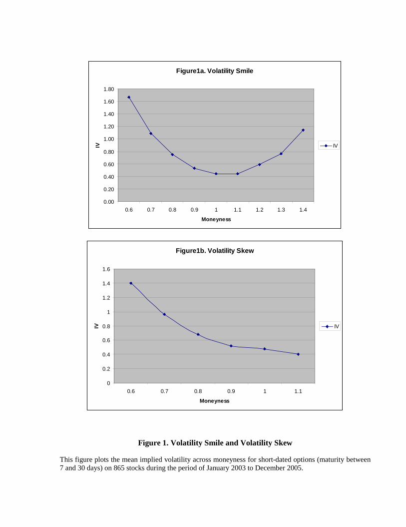
Figure1a. Volatility Smile
0.00
0.20
0.40
0.60
0.80
1.00
1.20
1.40
1.60
1.80
0.6 0.7 0.8 0.9 1 1.1 1.2 1.3 1.4
Moneyness
IV IV
Figure1b. Volatility Skew
0
0.2
0.4
0.6
0.8
1
1.2
1.4
1.6
0.6 0.7 0.8 0.9 1 1.1
Moneyness
IV IV
Figure 1. Volatility Smile and Volatility Skew
This figure plots the mean implied volatility across moneyness for short-dated options (maturity between 7 and 30 days) on 865 stocks during the period of January 2003 to December 2005.

43
Figure 2a. Smile Sample
0
0.2
0.4
0.6
0.8
1
1.2
1.4
7 8 9 10 11 14 15 16 17 18 21 22 23 24 25 28 29 30
Day-to-expiration
IV
OTM Put IVOTM Call IVATM IV
Figure 2b. Skew Sample
00.20.40.60.8
11.21.41.61.8
7 8 9 10 11 14 15 16 17 18 21 22 23 24 25 28 29 30
Day-to-expiration
IV
OTM Put IVATM IVOTM Call IV
Figure 2. Term Structure of the Implied Volatility
This figure plots the average implied volatility of options in each category with day-to-expiration. The sample contains options on 865 stocks over the period of January 2003 to December 2005.
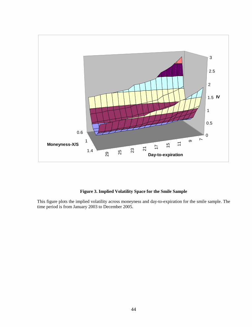
44
79
11151721232529
0.6
1
1.4
0
0.5
1
1.5
2
2.5
3
IV
Day-to-expiration
Moneyness-X/S
Figure 3. Implied Volatility Space for the Smile Sample
This figure plots the implied volatility across moneyness and day-to-expiration for the smile sample. The time period is from January 2003 to December 2005.