Helsinki June 20091 Confidence Intervals and Hypothesis Tests (Statistical Inference) Ian Jolliffe Introduction Illustrative Example Types of Inference

Helsinki June 2009 1

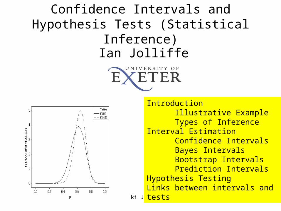
Confidence Intervals and Hypothesis Tests (Statistical Inference)

Ian Jolliffe

Introduction Illustrative ExampleTypes of Inference

Interval EstimationConfidence IntervalsBayes IntervalsBootstrap IntervalsPrediction Intervals

Hypothesis TestingLinks between intervals and tests


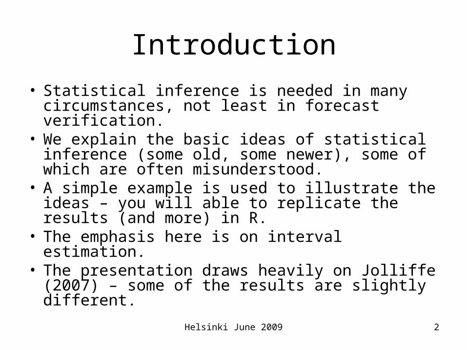
Introduction

• Statistical inference is needed in many circumstances, not least in forecast verification.

• We explain the basic ideas of statistical inference (some old, some newer), some of which are often misunderstood.

• A simple example is used to illustrate the ideas – you will able to replicate the results (and more) in R.

• The emphasis here is on interval estimation.• The presentation draws heavily on Jolliffe (2007)

– some of the results are slightly different.


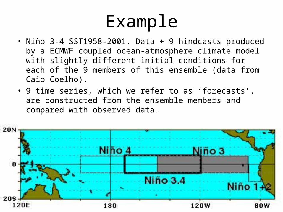
Example• Niño 3-4 SST1958-2001. Data + 9 hindcasts produced

by a ECMWF coupled ocean-atmosphere climate model with slightly different initial conditions for each of the 9 members of this ensemble (data from Caio Coelho).

• 9 time series, which we refer to as ‘forecasts’, are constructed from the ensemble members and compared with observed data.


Verification measures and uncertainty• We could compare the ‘forecasts’ with the observations

in a number of ways – for illustration consider – Compare the actual values of SST using the correlation

coefficient– Convert to binary data (is the SST above or below the mean?):

use hit rate (probability of detection - POD) as a verification measure.

• The values of these measures that we calculate have uncertainty associated with them – if we had a different set of forecasts and observations for Niño 3-4 SST, we would get different values.

• Assume that the data we have are a sample from some (hypothetical?) population and we wish to make inferences about the correlation and hit rate in that population.


Example - summary• The next two slides show

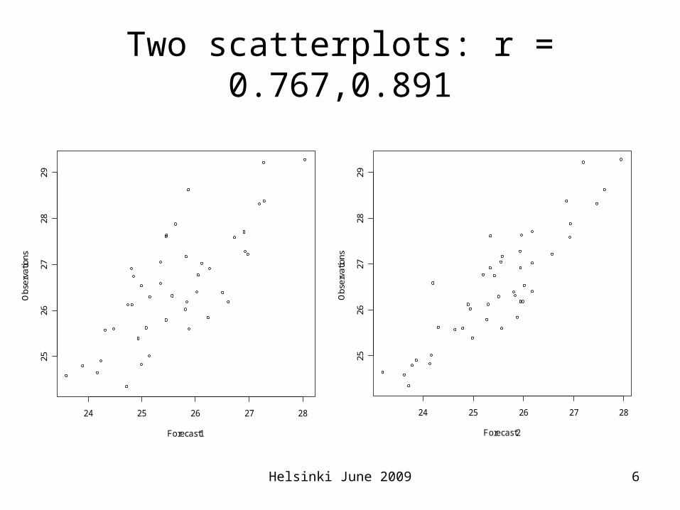
– Scatterplots of the observations against two of the forecasts (labelled Forecast 1, Forecast 2) with the lowest and highest correlations of the nine ‘forecasts’: r = 0.767, 0.891.

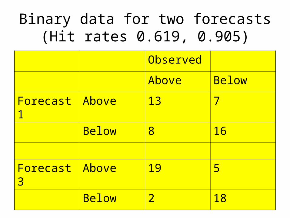
– Data tabulated according to whether they are above or below average, for two forecasts labelled Forecast 1, Forecast 3 with lowest and highest hit rates (PODs) 0.619, 0.905.

– The variation in values between these forecasts illustrates the need for quantifying uncertainty.

• We will look at various ways of making inferences based on these correlations and hit rates.


Two scatterplots: r = 0.767,0.891

24 25 26 27 28

2526

2728

29

Forecast2

Obs

erva

tions

24 25 26 27 28

2526

2728

29

Forecast1

Obs

erva

tions


Binary data for two forecasts(Hit rates 0.619, 0.905)

Observed

Above Below

Forecast 1 Above 13 7

Below 8 16


Below 2 18


Inference – the framework

• We have data that are considered to be a sample from some larger population.

• We wish to use the data to make inferences about some population quantities (parameters), for example population mean, variance, correlation, hit rate …


Types of inference

• Point estimation – e.g. simply give a single number to estimate the parameter, with no indication of the uncertainty associated with it.

• Interval estimation - a standard error could be attached to a point estimate, but it is better to go one step further and construct a confidence interval, especially if the distribution of the measure is not close to Gaussian.

• Hypothesis testing - in comparing estimates of a parameter for different samples, hypothesis testing may be a good way of addressing the question of whether any change could have arisen by chance.


Approaches to inference

1. Classical (frequentist) parametric inference.2. Bayesian inference.3. Non-parametric inference.4. Decision theory5. …Note that

– The likelihood function is central to both 1 and 2.– Computationally expensive techniques are of

increasing importance in both 2 and 3.For more, at a fairly advanced level, see Garthwaite et al. (2002).


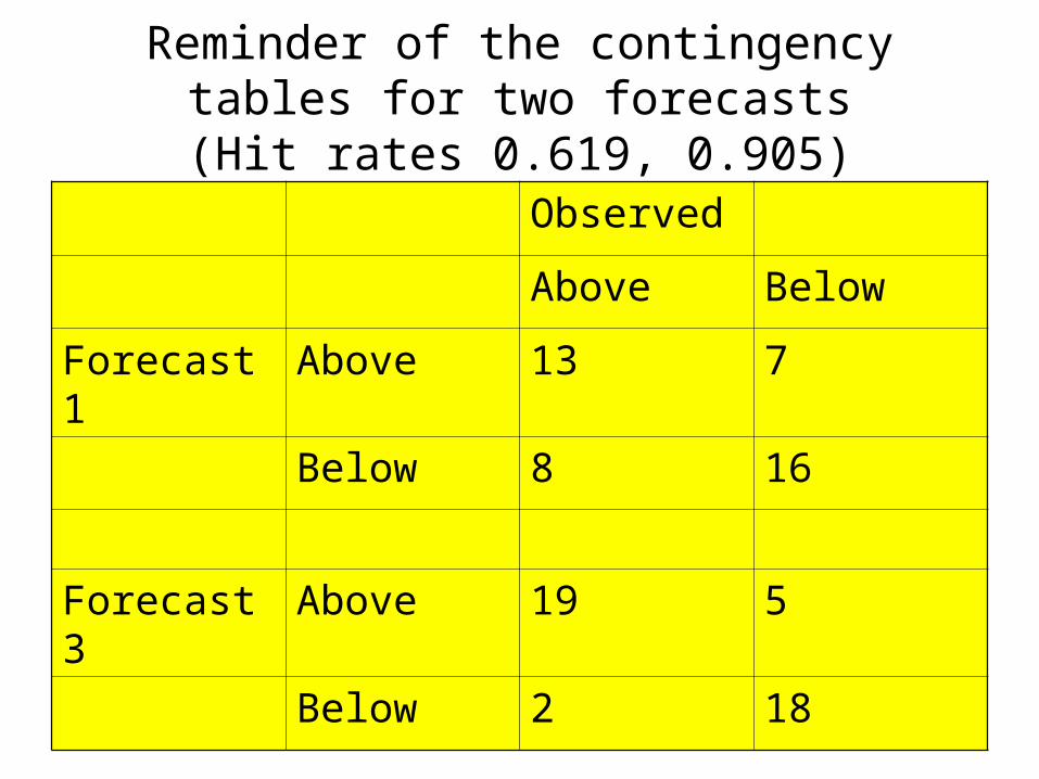
Reminder of the contingency tables for two forecasts

(Hit rates 0.619, 0.905)Observed

Above Below


Below 8 16


Below 2 18


Interval estimation

What is

• A confidence interval?

• A prediction or probability interval?

• A Bayes or credible interval?

• An interval obtained by bootstrapping?


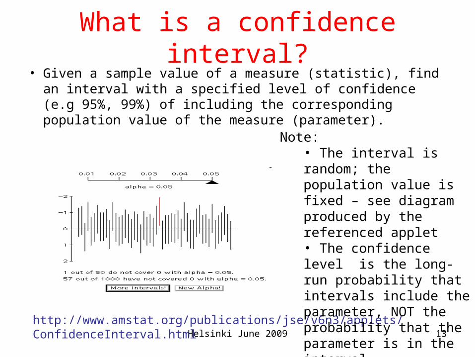
What is a confidence interval?• Given a sample value of a measure (statistic), find an

interval with a specified level of confidence (e.g 95%, 99%) of including the corresponding population value of the measure (parameter).

http://www.amstat.org/publications/jse/v6n3/applets/ConfidenceInterval.html

Note:• The interval is random; the population value is fixed – see diagram produced by the referenced applet• The confidence level is the long-run probability that intervals include the parameter, NOT the probability that the parameter is in the interval


Confidence intervals for hit rate

• Like several other verification measures, hit rate is the proportion of times that something occurs – in this case the proportion of occurrences of the event of interest that were forecast. Denote such a proportion by p.

• A confidence interval can be found for the underlying probability of a correct forecast, given that the event occurred. Call this probability .

• The situation is the standard one of finding a confidence interval for the ‘probability of success’ in a binomial distribution, and there are various ways of tackling this.


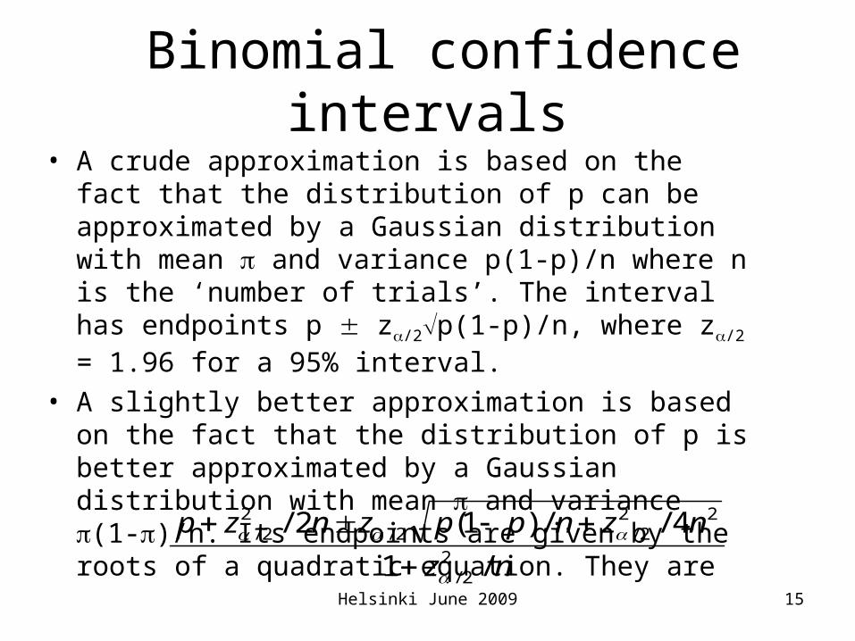
Binomial confidence intervals• A crude approximation is based on the fact that the

distribution of p can be approximated by a Gaussian distribution with mean and variance p(1-p)/n where n is the ‘number of trials’. The interval has endpoints p z/2p(1-p)/n, where z/2 = 1.96 for a 95% interval.

• A slightly better approximation is based on the fact that the distribution of p is better approximated by a Gaussian distribution with mean and variance (1-)/n. Its endpoints are given by the roots of a quadratic equation. They are

nz

nznppznzp

/1

4//)1(2/2

2/

222/2/

22/


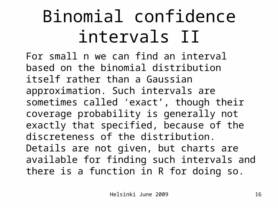
Binomial confidence intervals II

For small n we can find an interval based on the binomial distribution itself rather than a Gaussian approximation. Such intervals are sometimes called ‘exact’, though their coverage probability is generally not exactly that specified, because of the discreteness of the distribution. Details are not given, but charts are available for finding such intervals and there is a function in R for doing so.


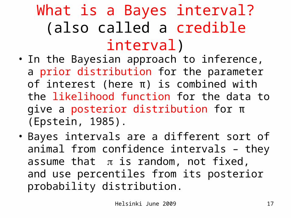
What is a Bayes interval? (also called a credible interval)

• In the Bayesian approach to inference, a prior distribution for the parameter of interest (here π) is combined with the likelihood function for the data to give a posterior distribution for π (Epstein, 1985).

• Bayes intervals are a different sort of animal from confidence intervals – they assume that is random, not fixed, and use percentiles from its posterior probability distribution.


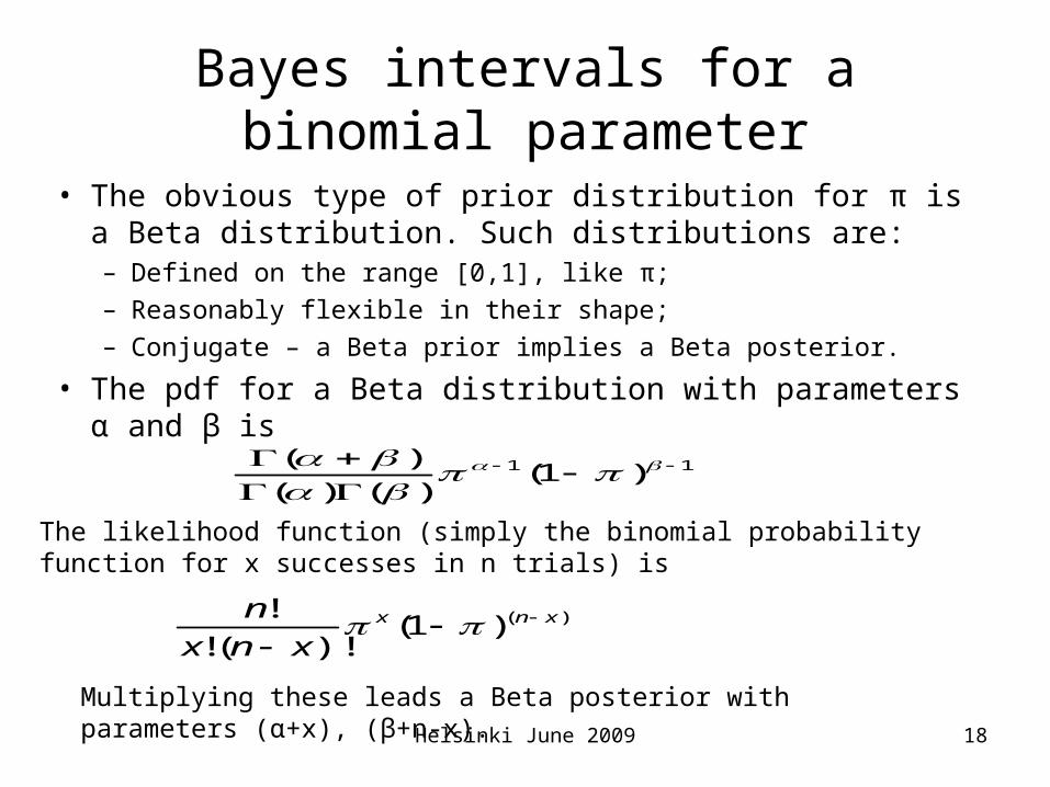
Bayes intervals for a binomial parameter

• The obvious type of prior distribution for π is a Beta distribution. Such distributions are:– Defined on the range [0,1], like π;

– Reasonably flexible in their shape;

– Conjugate – a Beta prior implies a Beta posterior.

• The pdf for a Beta distribution with parameters α and β is 11 )1(

)()(

)(

)()1()!(!

! xnx

xnx

n

The likelihood function (simply the binomial probability function for x successes in n trials) is

Multiplying these leads a Beta posterior with parameters (α+x), (β+n-x).


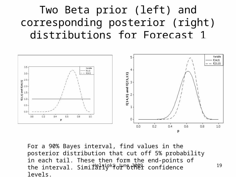
Two Beta prior (left) and corresponding posterior (right) distributions for Forecast 1

For a 90% Bayes interval, find values in the posterior distribution that cut off 5% probability in each tail. These then form the end-points of the interval. Similarly for other confidence levels.


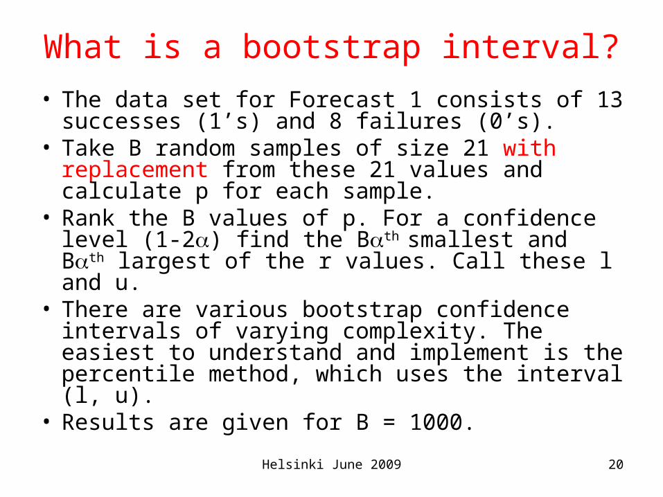
What is a bootstrap interval?

• The data set for Forecast 1 consists of 13 successes (1’s) and 8 failures (0’s).

• Take B random samples of size 21 with replacement from these 21 values and calculate p for each sample.

• Rank the B values of p. For a confidence level (1-2) find the Bth smallest and Bth largest of the r values. Call these l and u.

• There are various bootstrap confidence intervals of varying complexity. The easiest to understand and implement is the percentile method, which uses the interval (l, u).

• Results are given for B = 1000.


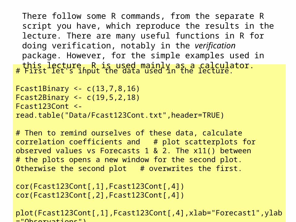
# First let's input the data used in the lecture.

Fcast1Binary <- c(13,7,8,16)Fcast2Binary <- c(19,5,2,18)Fcast123Cont <- read.table("Data/Fcast123Cont.txt",header=TRUE)

# Then to remind ourselves of these data, calculate correlation coefficients and # plot scatterplots for observed values vs Forecasts 1 & 2. The x11() between # the plots opens a new window for the second plot. Otherwise the second plot # overwrites the first.

cor(Fcast123Cont[,1],Fcast123Cont[,4])cor(Fcast123Cont[,2],Fcast123Cont[,4])

plot(Fcast123Cont[,1],Fcast123Cont[,4],xlab="Forecast1",ylab="Observations")x11() plot(Fcast123Cont[,2],Fcast123Cont[,4],xlab="Forecast2",ylab="Observations")

There follow some R commands, from the separate R script you have, which reproduce the results in the lecture. There are many useful functions in R for doing verification, notably in the verification package. However, for the simple examples used in this lecture, R is used mainly as a calculator.


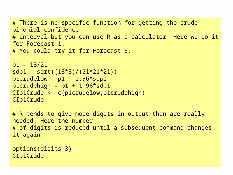
# There is no specific function for getting the crude binomial confidence# interval but you can use R as a calculator. Here we do it for Forecast 1.# You could try it for Forecast 3.

p1 = 13/21sdp1 = sqrt((13*8)/(21*21*21))p1crudelow = p1 - 1.96*sdp1p1crudehigh = p1 + 1.96*sdp1CIp1Crude <- c(p1crudelow,p1crudehigh)CIp1Crude

# R tends to give more digits in output than are really needed. Here the number # of digits is reduced until a subsequent command changes it again.

options(digits=3)CIp1Crude


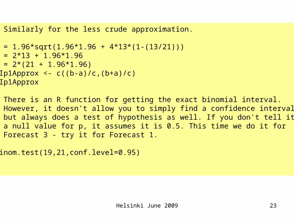
# Similarly for the less crude approximation.

a = 1.96*sqrt(1.96*1.96 + 4*13*(1-(13/21)))b = 2*13 + 1.96*1.96c = 2*(21 + 1.96*1.96)CIp1Approx <- c((b-a)/c,(b+a)/c)CIp1Approx

# There is an R function for getting the exact binomial interval. # However, it doesn't allow you to simply find a confidence interval # but always does a test of hypothesis as well. If you don't tell it # a null value for p, it assumes it is 0.5. This time we do it for # Forecast 3 - try it for Forecast 1.

binom.test(19,21,conf.level=0.95)


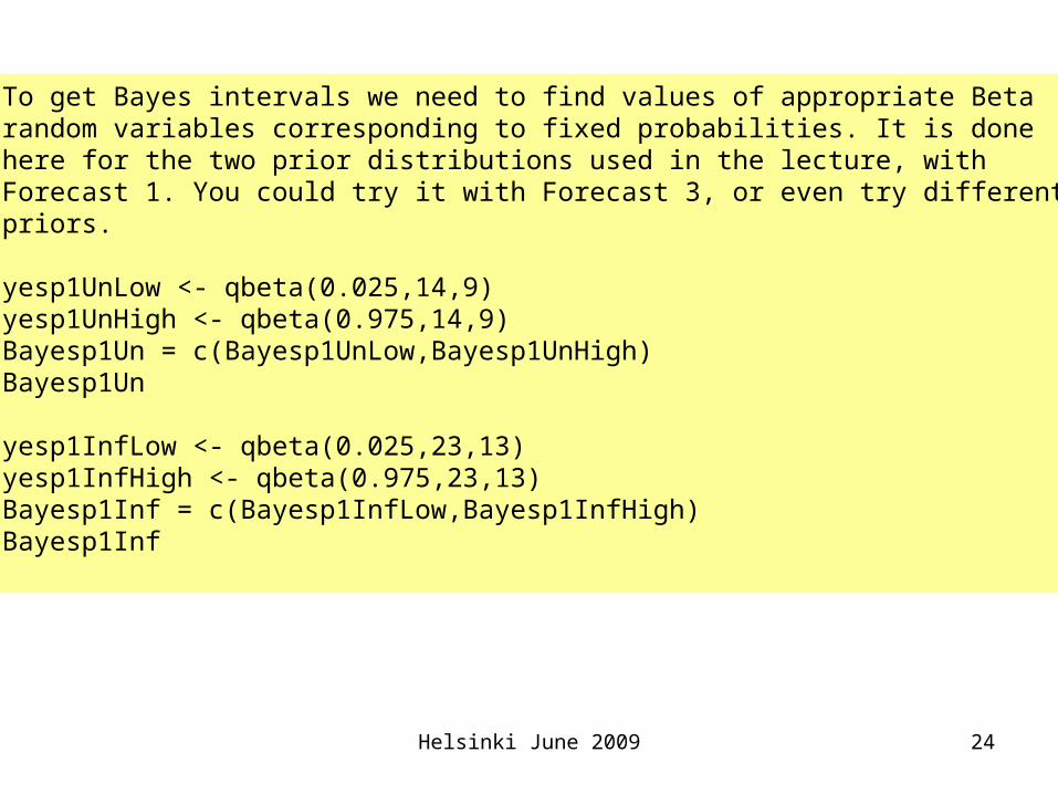
# To get Bayes intervals we need to find values of appropriate Beta # random variables corresponding to fixed probabilities. It is done # here for the two prior distributions used in the lecture, with # Forecast 1. You could try it with Forecast 3, or even try different # priors.

Bayesp1UnLow <- qbeta(0.025,14,9)Bayesp1UnHigh <- qbeta(0.975,14,9)CIBayesp1Un = c(Bayesp1UnLow,Bayesp1UnHigh)CIBayesp1Un

Bayesp1InfLow <- qbeta(0.025,23,13)Bayesp1InfHigh <- qbeta(0.975,23,13)CIBayesp1Inf = c(Bayesp1InfLow,Bayesp1InfHigh)CIBayesp1Inf


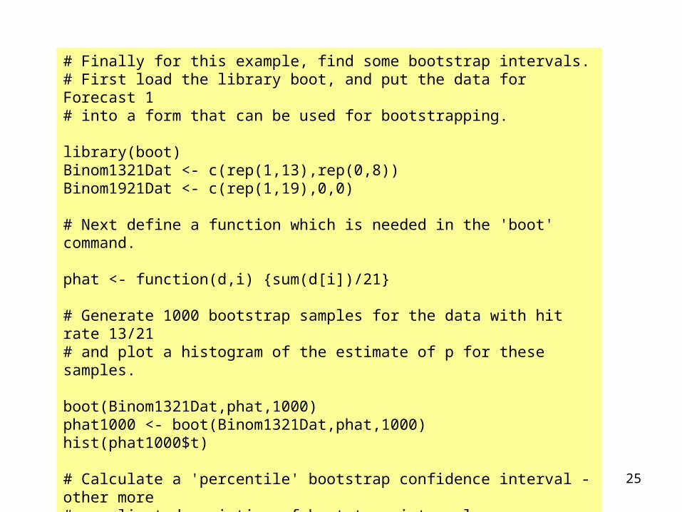
# Finally for this example, find some bootstrap intervals.# First load the library boot, and put the data for Forecast 1 # into a form that can be used for bootstrapping.

library(boot)Binom1321Dat <- c(rep(1,13),rep(0,8))Binom1921Dat <- c(rep(1,19),0,0)

# Next define a function which is needed in the 'boot' command.

phat <- function(d,i) {sum(d[i])/21}

# Generate 1000 bootstrap samples for the data with hit rate 13/21 # and plot a histogram of the estimate of p for these samples.

boot(Binom1321Dat,phat,1000)phat1000 <- boot(Binom1321Dat,phat,1000)hist(phat1000$t)

# Calculate a 'percentile' bootstrap confidence interval - other more # complicated varieties of bootstrap interval are available.

boot.ci(phat1000, conf=0.95, type = "perc")


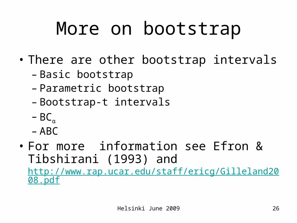
More on bootstrap

• There are other bootstrap intervals– Basic bootstrap – Parametric bootstrap– Bootstrap-t intervals– BCα

– ABC

• For more information see Efron & Tibshirani (1993) and http://www.rap.ucar.edu/staff/ericg/Gilleland2008.pdf

http://www.rap.ucar.edu/staff/ericg/Gilleland2008.pdf


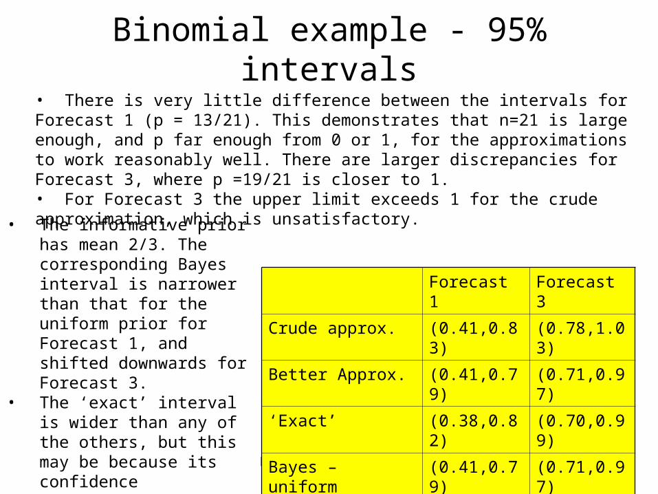
Binomial example - 95% intervals

Forecast 1 Forecast 3

Crude approx. (0.41,0.83) (0.78,1.03)

Better Approx. (0.41,0.79) (0.71,0.97)

‘Exact’ (0.38,0.82) (0.70,0.99)

Bayes – uniform (0.41,0.79) (0.71,0.97)

Bayes – informative (0.48,0.79) (0.66,0.92)

Percentile bootstrap (0.43,0.81) (0.76,1.00)

• There is very little difference between the intervals for Forecast 1 (p = 13/21). This demonstrates that n=21 is large enough, and p far enough from 0 or 1, for the approximations to work reasonably well. There are larger discrepancies for Forecast 3, where p =19/21 is closer to 1.• For Forecast 3 the upper limit exceeds 1 for the crude approximation, which is unsatisfactory.

• The informative prior has mean 2/3. The corresponding Bayes interval is narrower than that for the uniform prior for Forecast 1, and shifted downwards for Forecast 3.

• The ‘exact’ interval is wider than any of the others, but this may be because its confidence coefficient is greater than 95%.


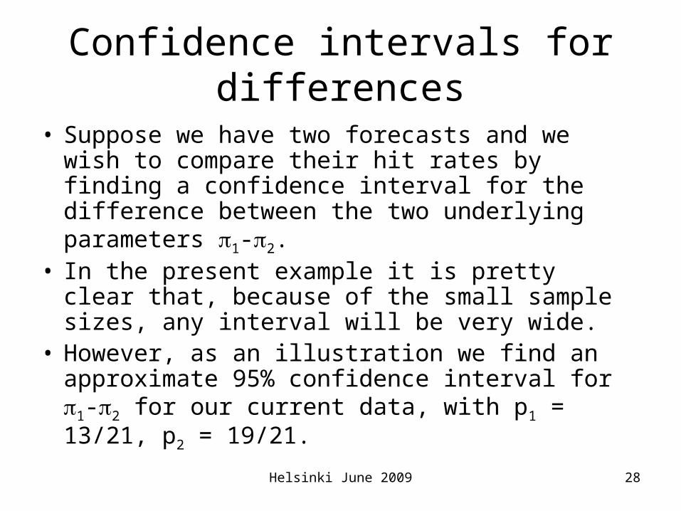
Confidence intervals for differences

• Suppose we have two forecasts and we wish to compare their hit rates by finding a confidence interval for the difference between the two underlying parameters 1-2.

• In the present example it is pretty clear that, because of the small sample sizes, any interval will be very wide.

• However, as an illustration we find an approximate 95% confidence interval for 1-2 for our current data, with p1 = 13/21, p2 = 19/21.


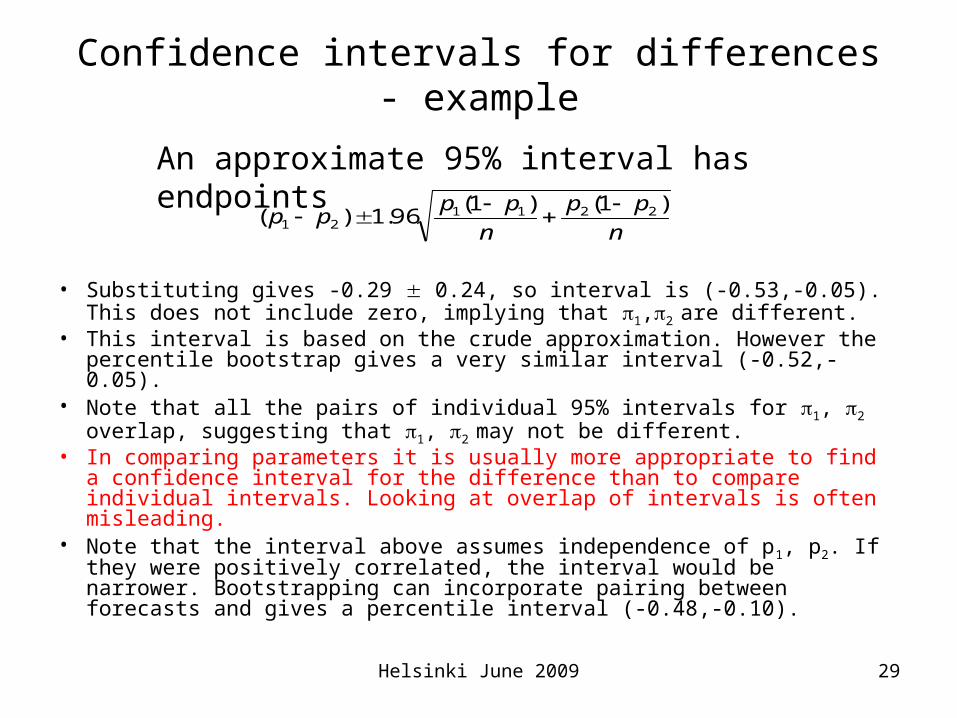
Confidence intervals for differences - example

• Substituting gives -0.29 0.24, so interval is (-0.53,-0.05). This does not include zero, implying that 1,2 are different.

• This interval is based on the crude approximation. However the percentile bootstrap gives a very similar interval (-0.52,-0.05).

• Note that all the pairs of individual 95% intervals for 1, 2 overlap, suggesting that 1, 2 may not be different.

• In comparing parameters it is usually more appropriate to find a confidence interval for the difference than to compare individual intervals. Looking at overlap of intervals is often misleading.

• Note that the interval above assumes independence of p1, p2. If they were positively correlated, the interval would be narrower. Bootstrapping can incorporate pairing between forecasts and gives a percentile interval (-0.48,-0.10).

An approximate 95% interval has endpoints

n

pp

n

pppp

)1()1(96.1)( 2211

21


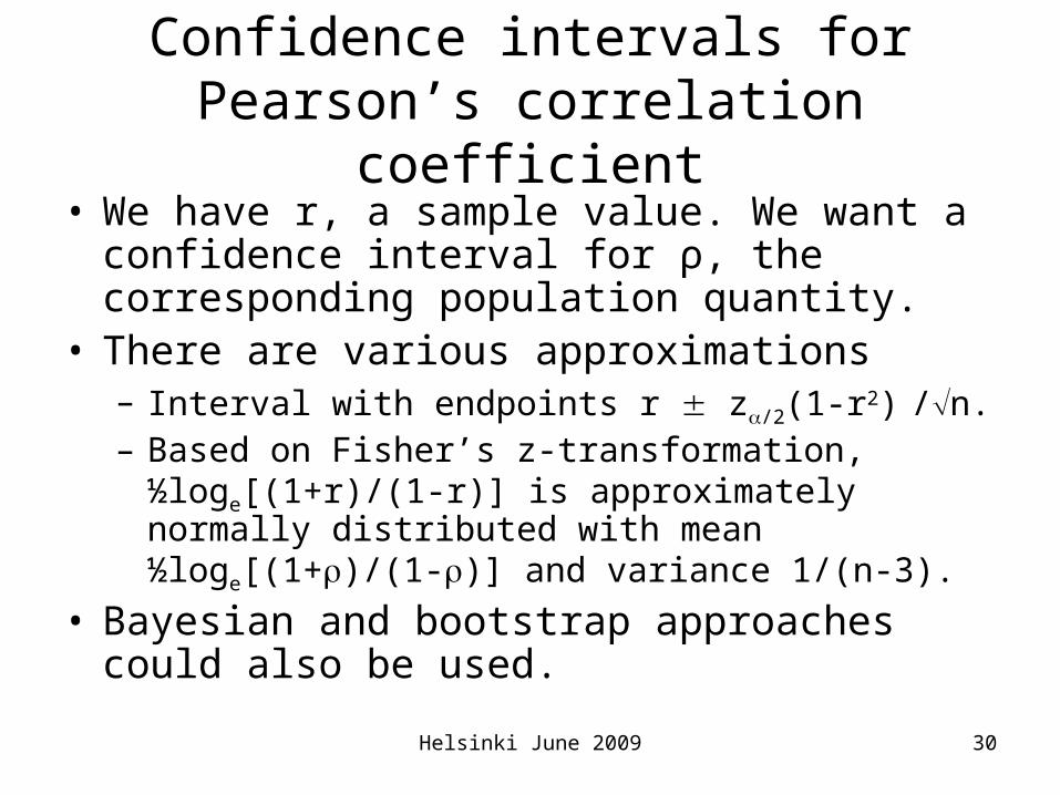
Confidence intervals for Pearson’s correlation coefficient

• We have r, a sample value. We want a confidence interval for ρ, the corresponding population quantity.

• There are various approximations– Interval with endpoints r z/2(1-r2) /n.– Based on Fisher’s z-transformation, ½loge[(1+r)/(1-r)]

is approximately normally distributed with mean ½loge[(1+)/(1-)] and variance 1/(n-3).

• Bayesian and bootstrap approaches could also be used.


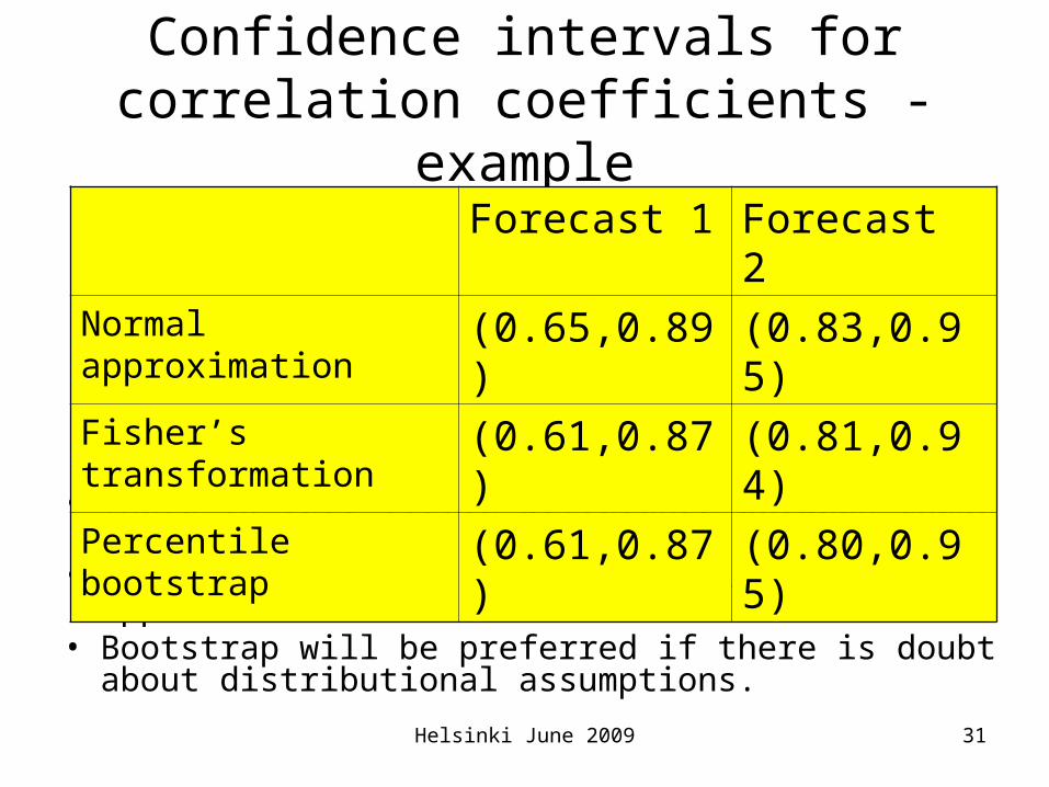
Confidence intervals for correlation coefficients - example

• There is very little difference between these intervals. • In general, the second should give a better approximation

than the first.• Bootstrap will be preferred if there is doubt about

distributional assumptions.

Forecast 1 Forecast 2

Normal approximation (0.65,0.89) (0.83,0.95)

Fisher’s transformation (0.61,0.87) (0.81,0.94)

Percentile bootstrap (0.61,0.87) (0.80,0.95)


What is a prediction interval?

• A prediction interval (or probability interval) is an interval with a given probability of containing the value of a random variable, rather than a parameter.

• The random variable is random and the interval’s endpoints are fixed points in its distribution, whereas the interval is random for a confidence interval.

• Prediction intervals, as well as confidence intervals, can be useful in quantifying uncertainty when estimating parameters.


Prediction intervals for correlation coefficients

• We need the distribution of r, usually calculated under some null hypothesis, the obvious one being that =0. Using the crudest approximation, r has a Gaussian distribution with mean zero, variance 1/n and a 95% prediction interval for r, given =0, has endpoints 0 1.961/n.

• Our example has n=44, so a 95% prediction interval is (-0.295, 0.295).

• Prediction interval: given ρ = 0 we are 95% confident that r lies in the interval (-0.295, 0.295).

• Confidence interval: given r = 0.767, we are 95% confident that the interval (0.61, 0.87) contains ρ.


Hypothesis testing

The interest in uncertainty associated with a verification measure is often of the form– Is the observed value compatible with what might

have been observed if the forecast system had no skill?

– Given two values of a measure for two different forecasting systems (or the same system at different times), could the difference in values have arisen by chance if there was no difference in underlying skill for the two systems (the two times)?


Hypothesis testing II

• Such questions can clearly be answered with a formal test of the null hypothesis of ‘no skill’ in the first case, or ‘equal skill’ in the second case.

• A test of hypothesis is often equivalent to a confidence interval and/or prediction interval.


Correlation coefficient - test of =0

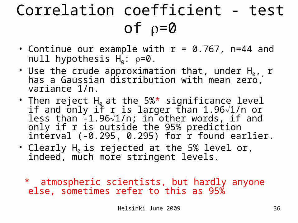
• Continue our example with r = 0.767, n=44 and null hypothesis H0: =0.

• Use the crude approximation that, under H0,, r has a Gaussian distribution with mean zero, variance 1/n.

• Then reject H0 at the 5%* significance level if and only if r is larger than 1.961/n or less than -1.961/n; in other words, if and only if r is outside the 95% prediction interval (-0.295, 0.295) for r found earlier.

• Clearly H0 is rejected at the 5% level or, indeed, much more stringent levels.

* atmospheric scientists, but hardly anyone else, sometimes refer to this as 95%


Correlation coefficient - test of =0 via confidence intervals

• We could also use any of our earlier confidence intervals to test H0. We gave 95% intervals, and would reject H0 at the 5% level if and only if the interval fails to include zero, which it does in all cases.

• If the intervals were 99%, the test would be at the 1% level, and so on. Similarly for prediction intervals.


Decision theory and p-values

• Hypothesis tests can be treated as a clear-cut decision process – decide on a significance level (5%, 1%) and derive a critical region (a subset of the possible data) for which some null hypothesis (H0) will be rejected.

• For a full decision theory approach, we also need a loss function and prior probabilities.

• Alternatively a p-value can be quoted. This is the probability that the data, or something less compatible with H0, could have arisen by chance if H0 was true.

• IT IS NOT the probability that H0 is true. • The latter can be found via a Bayesian approach.• For more on p-values, see Jolliffe (2004).


Permutation and randomisation tests of =0

• If we are not prepared to make assumptions about the distribution of r, we can use a permutation approach: – Denote the forecasts and observed data by (fi, oi), i =1, …n.– Fix the fis, and consider all possible permutations of the ois. – Calculate the correlation between the fis and permuted ois in

each case.– Under H0, all permutations are equally likely, and the p-value for

a permutation test is the proportion of all calculated correlations greater than or equal to (in absolute value for a two-sided test) the observed value.

• The number of permutations may be too large to evaluate them all. Using a random subset of them instead gives a randomisation test, though the terms permutation test and randomisation test are often used synonomously.


What have we learned?

• When calculating a verification measure, there is (almost?) always uncertainty associated with the value of that measure.

• Statistical inference can help to quantify that uncertainty.

• Sometimes we may wish to test a specific hypothesis such as ‘are the forecasts better than chance?’ or ‘does a new forecasting system give better forecasts than an old one?’.

• More often, a confidence interval, or some other type of interval, is a more useful way of quantifying uncertainty.


What have we learned II

• We have seen several different types of ‘uncertainty interval’: confidence intervals, Bayes intervals, bootstrap intervals, prediction intervals.

• For a given dataset, there may be different ways of calculating these intervals.

• The choice between intervals depends on the assumptions that can be made about the distribution of the data. Bootstrap (and other non-parametric) intervals typically make fewer assumptions than other intervals.

• We have also seen links between interval estimation and hypothesis testing.


Concluding (cautionary) remarks

• We have covered some of the main ideas, but only a tiny part, of statistical inference. For example, there was nothing on traditional non-parametric inference.

• Inference has many subtleties. The American Statistician often has examples of this in relatively simple contexts. For example, see Tuyl et al. (2008) for a discussion of what is an ‘uninformative’ prior distribution for a binomial parameter – a situation we considered.

• For some standard verification measures, software and/or formulae exist for quantifying uncertainty, but in many cases this is not yet the case. This is no excuse for ignoring uncertainty.


ReferencesEfron B and Tibshirani RJ (1993). An Introduction to the Bootstrap. New York:

Chapman & Hall.

Epstein ES (1985). Statistical Inference and Prediction in Climatology: A Bayesian Approach. Meteorological Monograph. American Meteorological Society.

Garthwaite PH, Jolliffe IT & Jones B (2002). Statistical Inference, 2nd edition. Oxford University Press.

Jolliffe IT (2004) P stands for … Weather, 59,77-79.

Jolliffe IT (2007). Uncertainty and inference for verification measures. Wea. Forecasting, 22, 637-650.

Tuyl F, Gerlach R & Mengersen K (2008). A comparison of Bayes-Laplace, Jeffreys, and other priors: the case of zero events. Amer. Statist., 62, 40-44.


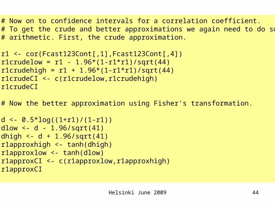
# Now on to confidence intervals for a correlation coefficient.# To get the crude and better approximations we again need to do some# arithmetic. First, the crude approximation.

r1 <- cor(Fcast123Cont[,1],Fcast123Cont[,4])r1crudelow = r1 - 1.96*(1-r1*r1)/sqrt(44)r1crudehigh = r1 + 1.96*(1-r1*r1)/sqrt(44)r1crudeCI <- c(r1crudelow,r1crudehigh)r1crudeCI

# Now the better approximation using Fisher's transformation.

d <- 0.5*log((1+r1)/(1-r1))dlow <- d - 1.96/sqrt(41)dhigh <- d + 1.96/sqrt(41)r1approxhigh <- tanh(dhigh)r1approxlow <- tanh(dlow)r1approxCI <- c(r1approxlow,r1approxhigh)r1approxCI


# R has a function that will provide a confidence interval for a correlation# coefficient but like that for a binomial parameter, the interval can only be # found in conjunction with a test of hypothesis. The result tallies with that # found above using Fisher's transformation.

cor.test(Fcast123Cont[,1],Fcast123Cont[,4],method = "pearson", conf.level = 0.95)

# Finally for the correlation coefficient we do a similar bootstrapping as # for the hit rate.

corr <- function(d,i) {cor(d[i,1],d[i,4])}boot(Fcast123Cont,corr,1000)corr1000 <- boot(Fcast123Cont,corr,1000)hist(corr1000$t)boot.ci(corr1000, conf=0.95,type = "perc")

# You can repeat all the confidence intervals above for Forecast 2 instead# of Forecast 1 by replacing Fcast123Cont[,1] by Fcast123Cont[,2] in # appropriate places above.


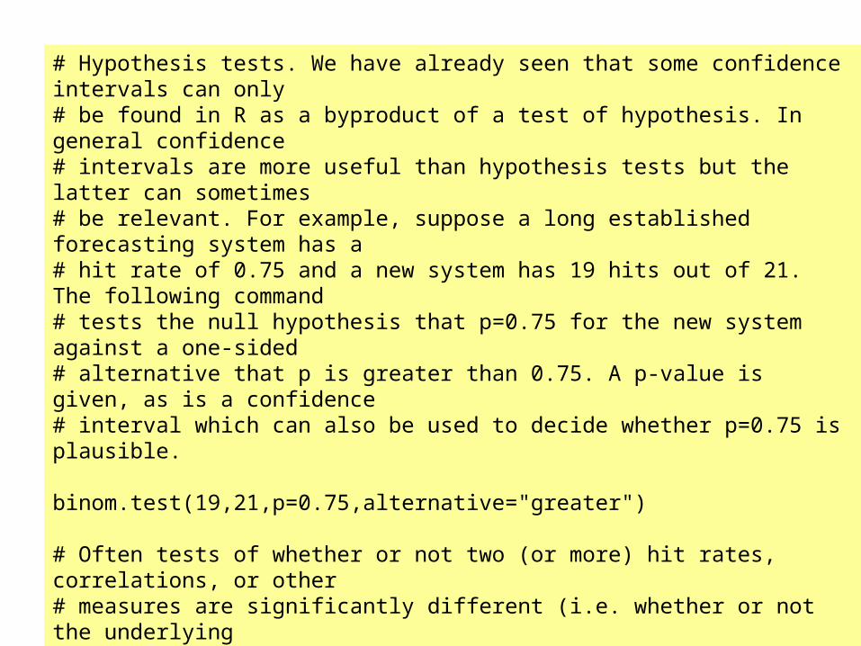
# Hypothesis tests. We have already seen that some confidence intervals can only# be found in R as a byproduct of a test of hypothesis. In general confidence # intervals are more useful than hypothesis tests but the latter can sometimes# be relevant. For example, suppose a long established forecasting system has a# hit rate of 0.75 and a new system has 19 hits out of 21. The following command# tests the null hypothesis that p=0.75 for the new system against a one-sided # alternative that p is greater than 0.75. A p-value is given, as is a confidence# interval which can also be used to decide whether p=0.75 is plausible.

binom.test(19,21,p=0.75,alternative="greater")

# Often tests of whether or not two (or more) hit rates, correlations, or other # measures are significantly different (i.e. whether or not the underlying# population difference is zero) are of interest. R has little that addresses this # directly. Here we use bootstrapping to compare two hit rates 13/21 and 19/21. # First create a data matrix from which we can sample.

HitRatesData <- c(Binom1321Dat,Binom1921Dat)HitRates.mat <- matrix(HitRatesData,21,2)


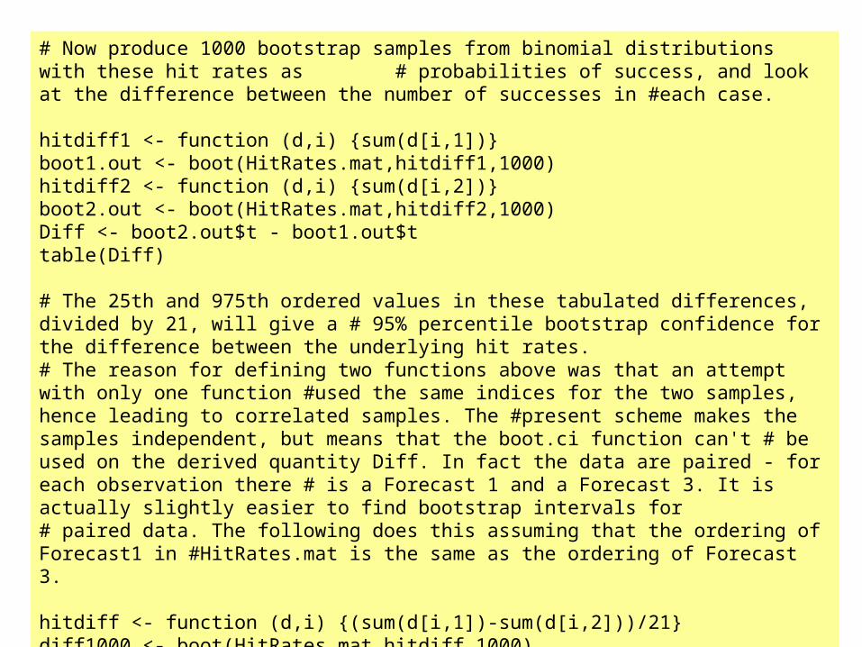
# Now produce 1000 bootstrap samples from binomial distributions with these hit rates as # probabilities of success, and look at the difference between the number of successes in #each case.

hitdiff1 <- function (d,i) {sum(d[i,1])}boot1.out <- boot(HitRates.mat,hitdiff1,1000)hitdiff2 <- function (d,i) {sum(d[i,2])}boot2.out <- boot(HitRates.mat,hitdiff2,1000)Diff <- boot2.out$t - boot1.out$ttable(Diff)

# The 25th and 975th ordered values in these tabulated differences, divided by 21, will give a # 95% percentile bootstrap confidence for the difference between the underlying hit rates.# The reason for defining two functions above was that an attempt with only one function #used the same indices for the two samples, hence leading to correlated samples. The #present scheme makes the samples independent, but means that the boot.ci function can't # be used on the derived quantity Diff. In fact the data are paired - for each observation there # is a Forecast 1 and a Forecast 3. It is actually slightly easier to find bootstrap intervals for # paired data. The following does this assuming that the ordering of Forecast1 in #HitRates.mat is the same as the ordering of Forecast 3.

hitdiff <- function (d,i) {(sum(d[i,1])-sum(d[i,2]))/21}diff1000 <- boot(HitRates.mat,hitdiff,1000)boot.ci(diff1000, conf=0.95,type = "perc")

Documents

Helsinki June 20091 Confidence Intervals and Hypothesis Tests (Statistical Inference) Ian Jolliffe Introduction Illustrative Example Types of Inference