HEDGING AND PORTFOLIO OPTIMIZATION UNDER TRANSACTION COSTS:A MARTINGALE APPROACH∗

by

JAKSA CVITANIC IOANNIS KARATZAS†

Department of Statistics Department of StatisticsColumbia University Columbia UniversityNew York, NY 10027 New York, NY 10027cj@stat.columbia.edu ik@stat.columbia.edu

Abstract

We derive a formula for the minimal initial wealth needed to hedge an arbitrary contingentclaim in a continuous-time model with proportional transaction costs; the expression ob-tained can be interpreted as the supremum of expected discounted values of the claim, overall (pairs of) probability measures under which the “wealth process” is a supermartingale.Next, we prove the existence of an optimal solution to the portfolio optimization problemof maximizing utility from terminal wealth in the same model; we also characterize thissolution via a transformation to a hedging problem: the optimal portfolio is the one thathedges the inverse of marginal utility evaluated at the shadow state-price density solv-ing the corresponding dual problem, if such exists. We can then use the optimal shadowstate-price density for pricing contingent claims in this market. The mathematical toolsare those of continuous-time martingales, convex analysis, functional analysis and dualitytheory.

Abbreviated Title: Transaction Costs

Revised Version, October 1995

Appeared in: Mathematical Finance 6 (1996), 113-165.

Key Words and Phrases: transaction costs, hedging, portfolio optimization,martingales, convex duality.AMS-MOS (1991) Subject Classifications: Primary 90A09, 90A12; secondary 60H30,93E20.

∗ Work supported in part by NSF Grants DMS-93-19816 and DMS-95-03582.† Part of this author’s work was carried out while visiting the Stochastic Analysis Group,

Australian National University, Canberra, and the Isaac Newton Institute for Mathemat-ical Sciences, University of Cambridge. He wishes to extend his thanks to his hosts fortheir hospitality.

1

1. INTRODUCTION.

We obtain a formula for the minimal initial wealth needed to hedge an arbitrary contingent

claim in a continuous-time model with proportional transaction costs. The expression

obtained can be interpreted as the supremum of expected values of the discounted value of

the claim, under all feasible “equivalent supermartingale measures”, namely the probability

measures under which an appropriate “discounted wealth process” is a supermartingale.

These results are similar in spirit to some of those obtained by Jouini & Kallal (1991) and,

in a discrete-time model, by Kusuoka (1995) and Shirakawa & Konno (1995). Unlike most

of the work on hedging under transaction costs (starting with Leland (1985)), we require

almost sure rather than just approximate hedge. In other words, the investor has to be

able to pay off the claim at the exercise time, no matter what the path of the stock-price

has been. This gives an upper bound for the claim price which is typically quite high.

For example, in the case of the European call, this mimimal hedging price is equal to

the price of the stock at the time the option is purchased (this result was conjectured

in Davis & Clark (1994) and was proved by Soner, Shreve & Cvitanic (1995), as well as

by Levental & Skorohod (1995)). Nevertheless, we find the result useful in studying the

portfolio optimization problem on a finite time-horizon, and also for a preference-based

method for pricing claims under transaction costs.

The methodology proceeds as follows. We characterize the solution to the portfo-

lio optimization problem of maximizing utility from terminal wealth in the model, via a

transformation to a hedging problem; the optimal portfolio is the one that hedges the

inverse of marginal utility, evaluated at the shadow state-price density which solves the

corresponding dual problem. This hedging-duality approach has been used previously in

models of incomplete markets, markets with constraints and markets with nonlinear drifts

in the wealth process of the investor (Cvitanic and Karatzas (1992, 1993)), but seems to

be new in the context of models with transaction costs. A related approach based on the

2

stochastic maximum principle for singular control problems, as developed in Cadenillas &

Haussman (1994), is suggested in Cadenillas & Haussman (1993). The typical approach

to utility maximization under transaction costs has been the analytical study of the value

function, and the description of the optimal strategy as one with no transactions in a

certain region, and with minimal transactions at the boundary in order always to keep the

holdings vector inside the region. Such was the spirit of the pioneering work of Magill and

Constantinides (1976), and of the more mathematical papers by Taksar, Klass & Assaf

(1988), Davis and Norman (1990), Shreve & Soner (1994). Those papers deal with the

consumption optimization problem on an infinite-horizon. The finite-horizon problem is

studied in Davis, Panas & Zariphopoulou (1993). Our approach gives different insights,

can be applied to the case of time-dependent and random market coefficients, but provides

no explicit description of optimal strategies, except for the cases in which it is optimal

not to trade at all. The latter is the case when the difference between the return rate

of the stock and the interest rate is nonnegative but small, and/or the time-horizon is

small relative to the transaction costs. This is in contrast with the infinite-horizon case, in

which it is always optimal to hold some money in the stock if the return rate is positive, no

matter how small it is. It should be of considerable interest, to find additional examples

that admit explicit solutions.

We also prove the existence of an optimal trading strategy directly, using standard

functional-analytic arguments, without imposing extra assumptions such as the existence

of an optimal solution to the dual problem.

Finally, we indicate how to use the optimization result for a utility-based approach

to the pricing of contingent claims in such a market. Namely, following the approach

of Davis (1994) as applied in Karatzas & Kou (1994), we use the price obtained as the

expected value of the claim under the probability measure corresponding to the optimal

shadow state-price density (in the dual problem), since with this price the investor becomes

3

neutral between diverting or not diverting a small amount of his funds into the option,

resulting in zero marginal rate of substitution.

Our model for proportional transaction costs is the same as that of Davis & Norman

(1990). We describe it precisely in Section 2, and define what we mean by hedging in this

market. We derive a formula for the minimal hedging price in Section 4, using the auxiliary

martingales (shadow state-price densities) introduced in Section 3. In Sections 5 and 6

we describe the utility maximization problem, characterize its solution, and present some

simple examples. Section 7 proposes a method for pricing contingent claims in a market

with transaction costs, using the optimal state-price density from the dual problem. The

long and technical proof of a closedness result for hedging strategies is provided in an

Appendix.

Here are some related works on the subject of transaction costs, that the reader may

find useful to consult: Avellaneda & Paras (1993), Bensaid, Lesne, Pages & Scheinkman

(1992), Boyle & Tan (1994), Boyle & Vorst (1992), Dewynne, Whalley & Wilmott (1993),

Davis & Panas (1994), Davis & Zariphopoulou (1995), Edirisinghe, Naik & Uppal (1993),

Figlewski (1989), Flesaker & Hughston (1994), Hodges & Clewlow (1993), Gilster & Lee

(1984), Henrotte (1993), Hodges & Neuberger (1989), Hoggard, Whalley & Wilmott (1993),

Merton (1989), Morton & Pliska (1993), Panas (1993), Pliska & Selby (1993), Shen (1990),

and Toft (1993).

2. THE MODEL; DEFINITION OF HEDGING.

We consider a financial market consisting of one riskless asset, called bank account (or

bond) with price B(·) given by

(2.1) dB(t) = B(t)r(t)dt, B(0) = 1;

and of one risky asset, called stock, with price-per-share S(·) governed by the stochastic

4

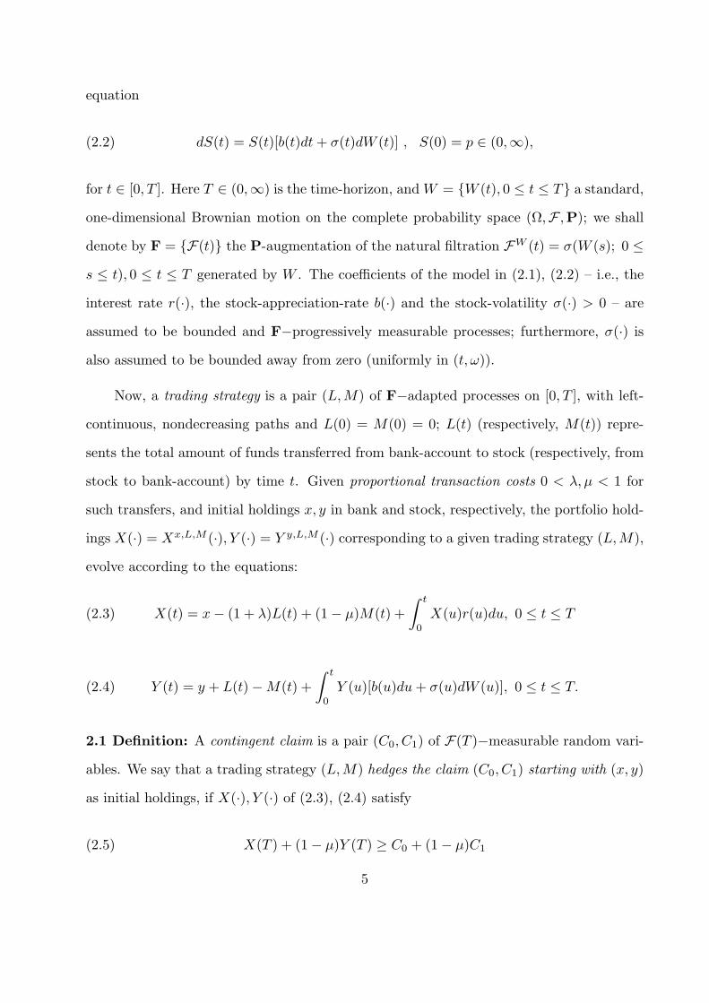
equation

(2.2) dS(t) = S(t)[b(t)dt + σ(t)dW (t)] , S(0) = p ∈ (0,∞),

for t ∈ [0, T ]. Here T ∈ (0,∞) is the time-horizon, and W = W (t), 0 ≤ t ≤ T a standard,

one-dimensional Brownian motion on the complete probability space (Ω,F ,P); we shall

denote by F = F(t) the P-augmentation of the natural filtration FW (t) = σ(W (s); 0 ≤s ≤ t), 0 ≤ t ≤ T generated by W . The coefficients of the model in (2.1), (2.2) – i.e., the

interest rate r(·), the stock-appreciation-rate b(·) and the stock-volatility σ(·) > 0 – are

assumed to be bounded and F−progressively measurable processes; furthermore, σ(·) is

also assumed to be bounded away from zero (uniformly in (t, ω)).

Now, a trading strategy is a pair (L,M) of F−adapted processes on [0, T ], with left-

continuous, nondecreasing paths and L(0) = M(0) = 0; L(t) (respectively, M(t)) repre-

sents the total amount of funds transferred from bank-account to stock (respectively, from

stock to bank-account) by time t. Given proportional transaction costs 0 < λ, µ < 1 for

such transfers, and initial holdings x, y in bank and stock, respectively, the portfolio hold-

ings X(·) = Xx,L,M (·), Y (·) = Y y,L,M (·) corresponding to a given trading strategy (L,M),

evolve according to the equations:

(2.3) X(t) = x− (1 + λ)L(t) + (1− µ)M(t) +∫ t

0

X(u)r(u)du, 0 ≤ t ≤ T

(2.4) Y (t) = y + L(t)−M(t) +∫ t

0

Y (u)[b(u)du + σ(u)dW (u)], 0 ≤ t ≤ T.

2.1 Definition: A contingent claim is a pair (C0, C1) of F(T )−measurable random vari-

ables. We say that a trading strategy (L,M) hedges the claim (C0, C1) starting with (x, y)

as initial holdings, if X(·), Y (·) of (2.3), (2.4) satisfy

(2.5) X(T ) + (1− µ)Y (T ) ≥ C0 + (1− µ)C1

5

(2.6) X(T ) + (1 + λ)Y (T ) ≥ C0 + (1 + λ)C1.

(Here and in the sequel, comparisons of random variables, in the form of equalities or

inequalities, are interpreted “almost surely”.)

Interpretation: Here C0 (respectively, C1) is understood as a target-position in the

bank-account (resp., the stock) at the terminal time t = T : for example

(2.7) C0 = −q1S(T )>q, C1 = S(T )1S(T )>q

in the case of a European call-option; and

(2.8) C0 = q1S(T )<q, C1 = −S(T )1S(T )<q

for a European put-option (both with exercise price q ≥ 0).

“Hedging”, in the sense of (2.5) and (2.6), simply means that “one is able to cover

these positions at t = T”. Indeed, assume that we have both Y (T ) ≥ C1 and (2.5), in the

form

(2.5)′ X(T ) + (1− µ)[Y (T )− C1] ≥ C0 ;

then (2.6) holds too, and (2.5)′ shows that we can cover the position in the bank-account

as well, by transferring the amount Y (T ) − C1 ≥ 0 to it. Similarly, suppose we have

Y (T ) < C1 and (2.6), in the form

(2.6)′ Y (T ) +1

1 + λ[X(T )− C0] ≥ C1 ;

then (2.5) holds as well, and (2.6)′ shows that we can again cover both positions by keeping

C0 in the bank-account and transferring the difference X(T )− C0 to the stock.

2.3 Remark: The equations (2.3), (2.4) can be written in the equivalent form

(2.9) d

(X(t)B(t)

)=

(1

B(t)

)[(1− µ)dM(t)− (1 + λ)dL(t)] , X(0) = x

6

(2.10) d

(Y (t)S(t)

)=

(1

S(t)

)[dL(t)− dM(t)] , Y (0) = y

in terms of “number-of-shares” (rather than amounts) held.

3. AUXILIARY MARTINGALES.

Consider the class D of pairs of strictly positive F−martingales (Z0(·), Z1(·)) with

(3.1) Z0(0) = 1 , z := Z1(0) ∈ [p(1− µ), p(1 + λ)]

and

(3.2) 1− µ ≤ R(t) :=Z1(t)

Z0(t)P (t)≤ 1 + λ, ∀ 0 ≤ t ≤ T,

where

(3.3) P (t) :=S(t)B(t)

= p +∫ t

0

P (u)[(b(u)− r(u))du + σ(u)dW (u)] , 0 ≤ t ≤ T

is the discounted stock price.

The martingales Z0(·), Z1(·) are the feasible state-price densities for holdings in bank

and stock, respectively, in this market with transaction costs; as such, they reflect the

“constraints” or “frictions” inherent in this market, in the form of condition (3.2). ¿From

the martingale representation theorem (e.g. Karatzas & Shreve (1991), §3.4) there exist

F−progressively measurable processes θ0(·), θ1(·) with∫ T

0(θ2

0(t) + θ21(t))dt < ∞ a.s. and

(3.4) Zi(t) = Zi(0) exp∫ t

0

θi(s)dW (s)− 12

∫ t

0

θ2i (s)ds

, i = 0, 1;

thus, the process R(·) of (3.2) has the dynamics

(3.5)dR(t) =R(t)[σ2(t) + r(t)− b(t)− (θ1(t)− θ0(t))(σ(t) + θ0(t))]dt

+ R(t)(θ1(t)− σ(t)− θ0(t))dW (t), R(0) = z/p.

7

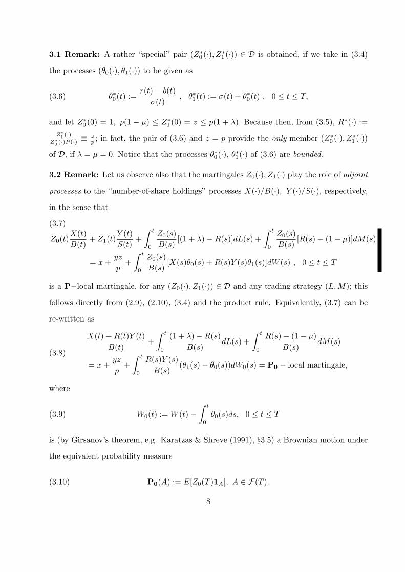
3.1 Remark: A rather “special” pair (Z∗0 (·), Z∗1 (·)) ∈ D is obtained, if we take in (3.4)

the processes (θ0(·), θ1(·)) to be given as

(3.6) θ∗0(t) :=r(t)− b(t)

σ(t), θ∗1(t) := σ(t) + θ∗0(t) , 0 ≤ t ≤ T,

and let Z∗0 (0) = 1, p(1 − µ) ≤ Z∗1 (0) = z ≤ p(1 + λ). Because then, from (3.5), R∗(·) :=Z∗1 (·)

Z∗0 (·)P (·) ≡ zp ; in fact, the pair of (3.6) and z = p provide the only member (Z∗0 (·), Z∗1 (·))

of D, if λ = µ = 0. Notice that the processes θ∗0(·), θ∗1(·) of (3.6) are bounded.

3.2 Remark: Let us observe also that the martingales Z0(·), Z1(·) play the role of adjoint

processes to the “number-of-share holdings” processes X(·)/B(·), Y (·)/S(·), respectively,

in the sense that

(3.7)

Z0(t)X(t)B(t)

+ Z1(t)Y (t)S(t)

+∫ t

0

Z0(s)B(s)

[(1 + λ)−R(s)]dL(s) +∫ t

0

Z0(s)B(s)

[R(s)− (1− µ)]dM(s)

= x +yz

p+

∫ t

0

Z0(s)B(s)

[X(s)θ0(s) + R(s)Y (s)θ1(s)]dW (s) , 0 ≤ t ≤ T

is a P−local martingale, for any (Z0(·), Z1(·)) ∈ D and any trading strategy (L,M); this

follows directly from (2.9), (2.10), (3.4) and the product rule. Equivalently, (3.7) can be

re-written as

(3.8)

X(t) + R(t)Y (t)B(t)

+∫ t

0

(1 + λ)−R(s)B(s)

dL(s) +∫ t

0

R(s)− (1− µ)B(s)

dM(s)

= x +yz

p+

∫ t

0

R(s)Y (s)B(s)

(θ1(s)− θ0(s))dW0(s) = P0 − local martingale,

where

(3.9) W0(t) := W (t)−∫ t

0

θ0(s)ds, 0 ≤ t ≤ T

is (by Girsanov’s theorem, e.g. Karatzas & Shreve (1991), §3.5) a Brownian motion under

the equivalent probability measure

(3.10) P0(A) := E[Z0(T )1A], A ∈ F(T ).

8

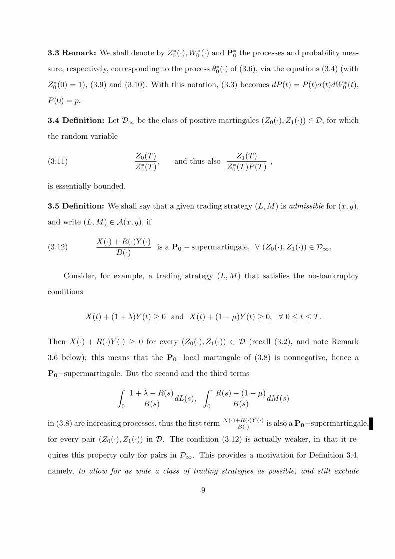
3.3 Remark: We shall denote by Z∗0 (·), W ∗0 (·) and P∗0 the processes and probability mea-

sure, respectively, corresponding to the process θ∗0(·) of (3.6), via the equations (3.4) (with

Z∗0 (0) = 1), (3.9) and (3.10). With this notation, (3.3) becomes dP (t) = P (t)σ(t)dW ∗0 (t),

P (0) = p.

3.4 Definition: Let D∞ be the class of positive martingales (Z0(·), Z1(·)) ∈ D, for which

the random variable

(3.11)Z0(T )Z∗0 (T )

, and thus alsoZ1(T )

Z∗0 (T )P (T ),

is essentially bounded.

3.5 Definition: We shall say that a given trading strategy (L,M) is admissible for (x, y),

and write (L,M) ∈ A(x, y), if

(3.12)X(·) + R(·)Y (·)

B(·) is a P0 − supermartingale, ∀ (Z0(·), Z1(·)) ∈ D∞.

Consider, for example, a trading strategy (L,M) that satisfies the no-bankruptcy

conditions

X(t) + (1 + λ)Y (t) ≥ 0 and X(t) + (1− µ)Y (t) ≥ 0, ∀ 0 ≤ t ≤ T.

Then X(·) + R(·)Y (·) ≥ 0 for every (Z0(·), Z1(·)) ∈ D (recall (3.2), and note Remark

3.6 below); this means that the P0−local martingale of (3.8) is nonnegative, hence a

P0−supermartingale. But the second and the third terms

∫ ·

0

1 + λ−R(s)B(s)

dL(s),∫ ·

0

R(s)− (1− µ)B(s)

dM(s)

in (3.8) are increasing processes, thus the first term X(·)+R(·)Y (·)B(·) is also a P0−supermartingale,

for every pair (Z0(·), Z1(·)) in D. The condition (3.12) is actually weaker, in that it re-

quires this property only for pairs in D∞. This provides a motivation for Definition 3.4,

namely, to allow for as wide a class of trading strategies as possible, and still exclude

9

arbitrage opportunities. This is usually done by imposing a lower bound on the wealth

process; however, that excludes simple strategies of the form “trade only once, by buying a

fixed number of shares of the stock at a specified time t”, which may require (unbounded)

borrowing. We shall have occasion, to use such strategies in the sequel; see, for example,

(4.20).

3.6 Remark: Here is a trivial (but useful) observation: if x + (1−µ)y ≥ a + (1−µ)b and

x + (1 + λ)y ≥ a + (1 + λ)b, then x + ry ≥ a + rb, ∀ 1− µ ≤ r ≤ 1 + λ.

4. HEDGING PRICE.

Suppose that we are given an initial holding y ∈ R in the stock, and want to hedge a given

contingent claim (C0, C1) with strategies which are admissible (in the sense of Definitions

2.1, 3.4). What is the smallest amount of holdings in the bank

(4.1) h(C0, C1; y) := infx ∈ R/ ∃(L,M) ∈ A(x, y) and (L,M) hedges (C0, C1)

that allows to do this? We call h(C0, C1; y) the hedging price of the contingent claim

(C0, C1) for initial holding y in the stock, and with the convention that h(C0, C1; y) = ∞if the set in (4.1) is empty.

Suppose this is not the case, and let x ∈ R belong to the set of (4.1); then for any

(Z0(·), Z1(·)) ∈ D∞ we have from (3.12), the Definition 2.1 of hedging, and Remark 3.6:

x +y

pEZ1(T ) = x +

y

pz ≥ E0

[X(T ) + R(T )Y (T )

B(T )

]

≥ E0

[C0 + R(T )C1

B(T )

]= E

[Z0(T )B(T )

(C0 + R(T )C1)]

,

so that x ≥ E[

Z0(T )B(T ) (C0 + R(T )C1)− y

pZ1(T )]. Therefore

(4.2) h(C0, C1; y) ≥ supD∞

E

[Z0(T )B(T )

(C0 + R(T )C1)− y

pZ1(T )

],

10

and this inequality is clearly also valid if h(C0, C1; y) = ∞.

4.1 Lemma: If the contingent claim (C0, C1) is bounded from below, in the sense

(4.3) C0 + (1 + λ)C1 ≥ −K and C0 + (1− µ)C1 ≥ −K, for some 0 ≤ K < ∞

then

(4.4)

supD∞

E

[Z0(T )B(T )

(C0 + R(T )C1)− y

pZ1(T )

]= sup

DE

[Z0(T )B(T )

(C0 + R(T )C1)− y

pZ1(T )

].

Proof: Start with arbitrary (Z0(·), Z1(·)) ∈ D and define the sequence of stopping times

τn ↑ T by

τn := inft ∈ [0, T ] /Z0(t)Z∗0 (t)

≥ n ∧ T, n ∈ N.

Consider also, for i = 0, 1 and in the notation of (3.6): θ(n)i (t) :=

θi(t), 0 ≤ t < τn

θ∗i (t), τn ≤ t ≤ T

and

Z(n)i (t) = zi exp

∫ t

0

θ(n)i (s)dW (s)− 1

2

∫ t

0

(θ(n)i (s))2ds

with z0 = 1, z1 = Z1(0) = EZ1(T ). Then, for every n ∈ N, both Z(n)0 (·) and Z

(n)1 (·) are

positive martingales, R(n)(·) = Z(n)1 (·)

Z(n)0 (·)P (·) = R(· ∧ τn) takes values in [1 − µ, 1 + λ] (by

(3.2) and Remark 3.1), and Z(n)0 (·)/Z∗0 (·) is bounded by n (in fact, constant on [τn, T ]).

Therefore, (Z(n)0 (·), Z(n)

1 (·)) ∈ D∞. Now let κ denote an upper bound on K/B(T ), and

observe, from Remark 3.6, (4.3) and Fatou’s lemma:

(4.5)

E

[Z0(T )B(T )

(C0 + R(T )C1)− y

pZ1(T )

]+

y

pZ1(0) + κ

= E

[Z0(T )

C0 + R(T )C1

B(T )+ κ

]

= E

[limn

Z(n)0 (T )

C0 + R(n)(T )C1

B(T )+ κ

]

≤ lim infn

E

[Z

(n)0 (T )

C0 + R(n)(T )C1

B(T )+ κ

]

= lim infn

E

[Z

(n)0 (T )B(T )

(C0 + R(n)(T )C1)− y

pZ

(n)1 (T )

]+

y

pZ1(0) + κ.

11

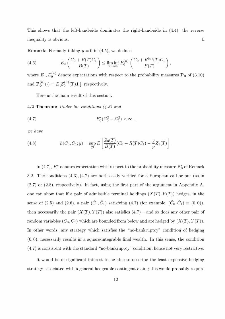
This shows that the left-hand-side dominates the right-hand-side in (4.4); the reverse

inequality is obvious.

Remark: Formally taking y = 0 in (4.5), we deduce

(4.6) E0

(C0 + R(T )C1

B(T )

)≤ lim inf

n→∞E

(n)0

(C0 + R(n)(T )C1

B(T )

),

where E0, E(n)0 denote expectations with respect to the probability measures P0 of (3.10)

and P(n)0 (·) = E[Z(n)

0 (T )1·], respectively.

Here is the main result of this section.

4.2 Theorem: Under the conditions (4.3) and

(4.7) E∗0 (C2

0 + C21 ) < ∞ ,

we have

(4.8) h(C0, C1; y) = supD

E

[Z0(T )B(T )

(C0 + R(T )C1)− y

pZ1(T )

].

In (4.7), E∗0 denotes expectation with respect to the probability measure P∗0 of Remark

3.2. The conditions (4.3), (4.7) are both easily verified for a European call or put (as in

(2.7) or (2.8), respectively). In fact, using the first part of the argument in Appendix A,

one can show that if a pair of admissible terminal holdings (X(T ), Y (T )) hedges, in the

sense of (2.5) and (2.6), a pair (C0, C1) satisfying (4.7) (for example, (C0, C1) ≡ (0, 0)),

then necessarily the pair (X(T ), Y (T )) also satisfies (4.7) – and so does any other pair of

random variables (C0, C1) which are bounded from below and are hedged by (X(T ), Y (T )).

In other words, any strategy which satisfies the “no-bankruptcy” condition of hedging

(0, 0), necessarily results in a square-integrable final wealth. In this sense, the condition

(4.7) is consistent with the standard “no-bankruptcy” condition, hence not very restrictive.

It would be of significant interest to be able to describe the least expensive hedging

strategy associated with a general hedgeable contingent claim; this would probably require

12

a purely probabilistic approach, using dynamic programming and control-theoretic ideas

coupled with martingale methods, in the spirit of our earlier work Cvitanic & Karatzas

(1993). Such a proof we have not been able to obtain. Our functional-analytic proof, which

takes up the remainder of this section and was inspired by similar arguments in Kusuoka

(1995), does not provide the construction of such a strategy.

Proof: In view of Lemma 4.1 and the inequality (4.2), it suffices to show

(4.9) h(C0, C1; y) ≤ supD

E

[Z0(T )

C0

B(T )+ Z1(T )

(C1

S(T )− y

p

)]=: R.

And in order to alleviate somewhat the (already rather heavy) notation, we shall take

p = 1, r(·) ≡ 0, thus B(·) ≡ 1, for the remainder of the section and in Appendix A; the

reader will verify easily that this entails no loss of generality.

We start by taking an arbitrary b < h(C0, C1; y) and considering the sets

(4.10)

A0 := (U, V ) ∈ (L∗2)2 : ∃(L,M) ∈ A(0, 0) that hedges (U, V ) starting with x = 0, y = 0

(4.11) A1 := (C0 − b, C1 − yS(T )),

where L∗2 = L2(Ω,F(T ),P∗0). It is not hard to prove (see below) that

(4.12) A0 is a convex cone, and contains the origin (0, 0), in (L∗2)2,

(4.13) A0 ∩A1 = ∅.

It is, however, considerably harder to establish that

(4.14) A0 is closed in (L∗2)2.

(This proof is carried out in Appendix A.) From (4.12)-(4.14) and the Hahn-Banach the-

orem there exists a pair of random variables (ρ∗0, ρ∗1) ∈ (L∗2)

2, not equal to (0, 0), such

that

(4.15) E∗0 [ρ∗0V0 + ρ∗1V1] = E[ρ0V0 + ρ1V1] ≤ 0, ∀ (V0, V1) ∈ A0

13

(4.16) E∗0 [ρ∗0(C0 − b) + ρ∗1(C1 − yS(T ))] = E[ρ0(C0 − b) + ρ1(C1 − yS(T ))] ≥ 0,

where ρi := ρ∗i Z∗0 (T ), i = 0, 1. It is also not hard to check (see below) that

(4.17) (1− µ)E[ρ0|F(t)] ≤ E[ρ1S(T )|F(t)]S(t)

≤ (1 + λ)E[ρ0|F(t)], ∀ 0 ≤ t ≤ T

(4.18) ρ1 ≥ 0, ρ0 ≥ 0 and Eρ0 > 0, E(ρ1S(T )) > 0.

In view of (4.18), we may take Eρ0 = 1, and then (4.16) gives

(4.19) b ≤ E[ρ0C0 + ρ1(C1 − yS(T ))].

Consider now arbitrary 0 < ε < 1, (Z0(·), Z1(·)) ∈ D, and define

Z0(t) := εZ0(t) + (1− ε)E[ρ0|F(t)], Z1(t) := εZ1(t) + (1− ε)E[ρ1S(T )|F(t)], 0 ≤ t ≤ T.

Clearly these are positive martingales, and Z0(0) = 1; on the other hand, multiplying in

(4.17) by 1 − ε, and in (1 − µ)Z0(t) ≤ Z1(t)/S(t) ≤ (1 + λ)Z0(t), 0 ≤ t ≤ T (just (3.2)

with r(·) ≡ 0) by ε, and adding up, we obtain (Z0(·), Z1(·)) ∈ D. Thus, in the notation of

(4.9),

R ≥ E

[Z0(T )C0 + Z1(T )

(C1

S(T )− y

)]

= (1− ε)E[ρ0C0 + ρ1(C1 − yS(T ))] + εE

[Z0(T )C0 + Z1(T )

(C1

S(T )− y

)]

≥ b(1− ε) + εE

[Z0(T )C0 + Z1(T )

(C1

S(T )− y

)]

from (4.19); letting ε ↓ 0 and then b ↑ h(C0, C1; y), we obtain (4.9), as required to complete

the proof of Theorem 4.2.

Proof of (4.12): Suppose that (Ui, Vi) ∈ (L∗2)2 are hedged by (Li,Mi) ∈ A(0, 0), respec-

tively, for i = 1, 2; in other words, if we let (Xi, Yi) be the corresponding holdings as in

(2.3), (2.4) (with x = y = 0, r(·) ≡ 0), we have:

Xi(T ) + (1− µ)Yi(T ) ≥ Ui + (1− µ)Vi,

14

Xi(T ) + (1 + λ)Yi(T ) ≥ Ui + (1 + λ)Vi,

and Xi(·) + R(·)Yi(·) is a P0−supermartingale, ∀ (Z0(·), Z1(·)) ∈ D∞ for i = 1, 2. Now,

with ζ ≥ 0, η ≥ 0 and (U, V ) = (ζU1 + ηU2, ζV1 + ηV2) ∈ (L∗2)2, it is straightforward to see

(using the linearity of the equations (2.3) and (2.4)) that (U, V ) is hedged by (L,M) =

(ζL1 +ηL2, ζM1 +ηM2) ∈ A(0, 0). If we take 0 < η < 1, ζ = 1−η we verify the convexity

of A0; if we take η > 0, ζ = 0 we verify that A0 is a cone; and we can hedge (0, 0) ∈ (L∗2)2

simply by L ≡ M ≡ 0.

Proof of (4.13): Suppose that A0∩A1 is not empty, i.e., that there exists (L,M) ∈ A(0, 0)

such that, with X(·) = X0,L,M (·) and Y (·) = Y 0,L,M (·), the process X(·) + R(·)Y (·) is a

P0−supermartingale for every (Z0(·), Z1(·)) ∈ D∞, and we have:

X(T ) + (1− µ)Y (T ) ≥ (C0 − b) + (1− µ)(C1 − yS(T )),

X(T ) + (1 + λ)Y (T ) ≥ (C0 − b) + (1 + λ)(C1 − yS(T )).

But then, with

X(·) := Xb,L,M (·) = b + X(·), Y (·) := Y y,L,M (·) = Y (·) + yS(·)

we have, from above, that X(·) + R(·)Y (·) = X(·) + R(·)Y (·) + b + yZ1(·)/Z0(·) is a

P0−supermartingale for every (Z0(·), Z1(·)) ∈ D∞, and that

X(T ) + (1− µ)Y (T ) ≥ C0 + (1− µ)C1,

X(T ) + (1 + λ)Y (T ) ≥ C0 + (1 + λ)C1.

In other words, (L, M) belongs to A(b, y) and hedges (C0, C1) starting with (b, y) – a

contradiction to the definition (4.1), and to the fact h(C0, C1; y) > b.

Proof of (4.17), (4.18): Fix t ∈ [0, T ) and let ξ be an arbitrary bounded, nonnegative,

F(t)−measurable random variable. Consider the strategy of starting with (x, y) = (0, 0)

15

and buying ξ shares of stock at time s = t, otherwise doing nothing (“buy-and-hold

strategy”); more explicitly, M ξ(·) ≡ 0, Lξ(s) = ξS(t)1(t,T ](s) and thus

(4.20)

Xξ(s) := X0,Lξ,Mξ

(·) = −ξ(1 + λ)S(t)1(t,T ](s), Y ξ(s) := Y 0,Lξ,Mξ

(s) = ξS(s)1(t,T ](s),

for 0 ≤ s ≤ T . Consequently, Z0(s)[Xξ(s)+R(s)Y ξ(s)] = ξ[Z1(s)−(1+λ)S(t)Z0(s)]1(t,T ](s)

is a P−supermartingale for every (Z0(·), Z1(·)) ∈ D, since, for instance with t < s ≤ T :

E[Z0(s)(Xξ(s) + R(s)Y ξ(s))|F(t)] = ξ (E[Z1(s)|F(t)]− (1 + λ)S(t)E[Z0(s)|F(t)])

= ξ[Z1(t)− (1 + λ)S(t)Z0(t)] = ξS(t)Z0(t)[R(t)− (1 + λ)] ≤ 0 = Z0(t)[Xξ(t) + R(t)Y ξ(t)].

Therefore, (Lξ,M ξ) ∈ A(0, 0), thus (Xξ(T ), Y ξ(T )) belongs to the set A0 of (4.10), and,

from (4.15):

0 ≥ E[ρ0Xξ(T ) + ρ1Y

ξ(T )] = E[ξ(ρ1S(T )− (1 + λ)ρ0S(t))]

= E[ξ(E[ρ1S(T )|F(t)]− (1 + λ)S(t)E[ρ0|F(t)]

)].

¿From the arbitrariness of ξ ≥ 0, we deduce the inequality of the right-hand side in

(4.17), and a dual argument gives the inequality of the left-hand side, for given t ∈ [0, T ).

Now all three processes in (4.17) have continuous paths (recall that martingales of the

Brownian filtration are representable as stochastic integrals, and thus have almost all

paths continuous); consequently, (4.17) is valid for all t ∈ [0, T ].

Next, we notice that (4.17) with t = T implies (1 − µ)ρ0 ≤ ρ1 ≤ (1 + λ)ρ0, so that

ρ0, hence also ρ1, is nonnegative. Similarly, (4.17) with t = 0 implies (1 − µ)Eρ0 ≤E[ρ1S(T )] ≤ (1+λ)Eρ0, and therefore, since (ρ0, ρ1) is not equal to (0, 0), Eρ0 > 0, hence

also E[ρ1S(T )] > 0. This proves (4.18).

4.3 Example: Consider the European call option of (2.7), whereby one has to deliver a

share of the stock if the price S(T ) at time t = T exceeds q, and one can still cover the

remaining position in the bank by the amount q > 0 of the exercise price. ¿From (4.8)

16

with y = 0, we have

(4.21) h(C0, C1) ≡ h(C0, C1; 0) = supD

E

[Z1(T )1S(T )>q − q

Z0(T )B(T )

1S(T )>q

],

and therefore, h(C0, C1) ≤ supD EZ1(T ) = supD Z1(0) ≤ (1 + λ)p. The number p(1 + λ)

corresponds to the cost of the “buy-and-hold strategy”, of acquiring one share of the stock

at t = 0 (at a price p(1+λ), due to the transaction cost), and holding on to it until t = T.

Davis & Clark (1993) conjectured that this hedging strategy is actually the cheapest:

(4.22) h(C0, C1) = (1 + λ)p.

The conjecture (4.22) was proved by Soner, Shreve & Cvitanic (1995), as well as by Levental

& Skorohod (1995). It is an open question to derive (4.22) directly from the representation

(4.21); in other words, to find a sequence (Z(n)0 (·), Z(n)

1 (·))n∈N with

P0(n)[S(T ) > q] → 0, E[Z(n)

1 (T )1S(T )>q] → 1, Z(n)1 (0) → 1 + λ,

as n ↑ ∞. We have not yet been able to accomplish this.

5. UTILITY FUNCTIONS.

In the next section we shall use the basic result, Theorem 4.2, to discuss some expected-

utility-maximization problems in the context of the model of section 2. For this, we shall

need the concept of utility function.

A function U : (0,∞) → R will be called utility function if it is strictly increasing,

strictly concave, contnuously differentiable, and satisfies

(5.1) U ′(0+) := limx↓0

U ′(x) = ∞ , U ′(∞) := limx→∞

U ′(x) = 0 .

We shall understand U(x) = −∞ for x < 0.

17

The continuous, strictly decreasing function U ′(·) has an inverse I(·) with these same

properties, which maps (0,∞) onto itself, and satisfies I(0+) = ∞, I(∞) = 0. We shall

also find useful the convex dual

(5.2) U(ζ) := maxx>0

[U(x)− xζ] = U(I(ζ))− ζI(ζ), 0 < ζ < ∞

of U(·), which satisfies

(5.3) U ′(ζ) = −I(ζ), 0 < ζ < ∞

Remark: For some purposes, we shall need to impose the extra condition

(5.4) xU ′(x) ≤ a + (1− b)U(x), ∀ 0 < x < ∞

(for suitable a ≥ 0, 0 < b ≤ 1) on our utility functions. This condition is clearly satisfied

by U(x) = log x and by U(x) = 1δ xδ, for 0 < δ < 1; it is also satisfied if U(∞) = ∞ and

U(·) is bounded from below (cf. Cuoco (1994)).

6. MAXIMIZING EXPECTED UTILITY FROM TERMINAL WEALTH.

Consider now a small investor, who can make decisions in the context of the market model

of (2.1), (2.2) as described in section 2, and who derives utility U(X(T+)) from his terminal

wealth

(6.1) X(T+) := X(T ) + f(Y (T )), where f(u) :=

(1 + λ)u ; u ≤ 0(1− µ)u ; u > 0

.

In other words, this agent liquidates at the end of the day his position in the stock, incurs

the appropriate transaction cost, and collects all the money in the bank-account. For a

given initial holding y ≥ 0 in the stock, his optimization problem is to find an admissible

pair (L, M) ∈ A+(x, y) that maximizes expected utility from terminal wealth, i.e., attains

the supremum

(6.2) V (x; y) := sup(L,M)∈A+(x,y)

EU(Xx,L,M (T ) + f(Y y,L,M (T ))

), 0 < x < ∞,

18

whereA+(x, y) is the class of processes (L,M) ∈ A(x, y) for which Xx,L,M (T )+f(Y y,L,M (T ))

≥ 0. We show in Appendix B that the supremum of (6.2) is attained, i.e., that there exists

an optimal pair (L, M) for this problem, and that V (x, y) < ∞. Our purpose in this

section is to describe the nature of this optimal pair, by using results of section 4 in the

context of the dual problem

(6.3) V (ζ; y) := inf(Z0,Z1)∈D

E

[U

(ζZ0(T )B(T )

)+

y

pζZ1(T )

], 0 < ζ < ∞,

under the following assumption.

6.1 Assumption: There exists a pair (Z0(·), Z1(·)) ∈ D, that attains the infimum in (6.3),

and does so for all 0 < ζ < ∞. Moreover, for all 0 < ζ < ∞, we have

V (ζ; y) < ∞ and E

[Z0(T )B(T )

I

(ζZ∗0 (T )B(T )

)]< ∞.

6.2 Remark: The assumption that the infimum of (6.3) is attained is a big one; we

have not yet been able to obtain a general existence result to this effect, only very simple

examples that can be solved explicitly (cf. Examples 6.5-6.7). The assumption that the

minimization in (6.3) can be carried out for all 0 < ζ < ∞ simultaneously, is made only

for simplicity; it can be dispensed with using methods analogous to those in Cvitanic &

Karatzas (1992). Note, however, that this latter assumption is satisfied if y = 0 and either

U(x) = log x or U(x) = 1δ xδ for 0 < δ < 1. It should also be mentioned that the optimal

pair (Z0(·), Z1(·)) of Assumption 6.1 need not be unique (we thank the anonimous referee

for pointing this out); thus, in the remainder of this section, (Z0(·), Z1(·)) will denote any

pair that attains the infimum in (6.3), as in Assumption 6.1

For any such pair, we have then the following property, proved at the end of this

section.

6.3 Lemma: Under the Assumption 6.1 and the condition (5.4), we have

(6.4)

E

[Z0(T )B(T )

I

(ζZ0(T )B(T )

)− y

pZ1(T )

]≤ E

[Z0(T )B(T )

I

(ζZ0(T )B(T )

)− y

pZ1(T )

]< ∞, ∀0 < ζ < ∞

19

for every (Z0(·), Z1(·)) in D.

Now, because the function ζ 7→ E[

Z0(T )B(T ) I(ζ Z0(T )

B(T ) )]

: (0,∞) → (0,∞) is continuous

and strictly decreasing, there exists a unique ζ = ζ(x; y, U) ∈ (0,∞) that satisfies

(6.5) E

[Z0(T )B(T )

I

(ζZ0(T )B(T )

)]= x +

y

pEZ1(T ).

And with

(6.6) C0 := I

(ζZ0(T )B(T )

), C1 := 0,

it follows from (6.4) that

(6.7)

sup(Z0,Z1)∈D

E

[Z0(T )

C0

B(T )+ Z1(T )

(C1

S(T )− y

p

)]= E

[Z0(T )

C0

B(T )+ Z1(T )

(C1

S(T )− y

p

)]

= x.

Consequently, if in addition we have C0 ∈ L∗2, then Theorem 4.2 gives h(C0, C1; y) = x.

Now it can be shown, by an argument analogous to that in the Appendix A (see also

the appendix in Soner, Shreve & Cvitanic (1995)), that the infimum in (4.1) is actually

attained; in other words, there exists a pair (L, M) ∈ A(x, y) such that, with X(·) ≡Xx,L,M (·), Y (·) ≡ Y y,L,M (·), we have

(6.8) X(T ) + (1− µ)Y (T ) ≥ C0, X(T ) + (1 + λ)Y (T ) ≥ C0.

6.4 Theorem: Under Assumption 6.1, and the conditions (5.4),

(6.9) E∗0 [C2

0 ] = E∗0

[I2(ζZ0(T )/B(T ))

]< ∞,

the above pair (L, M) ∈ A(x, y) is optimal for the problem of (6.2), and satisfies

(6.10) X(T+) := X(T ) + f(Y (T )) = I(ζZ0(T )/B(T )) = C0

(6.11) L(·) is flat off the set 0 ≤ t ≤ T/R(t) = 1 + λ

20

(6.12) M(·) is flat off the set 0 ≤ t ≤ T/R(t) = 1− µ

(6.13)X(t) + R(t)Y (t)

B(t)= E0

[I(ζZ0(T )/B(T ))

B(T )

∣∣∣∣F(t)

], 0 ≤ t ≤ T,

where R(·) := Z1(·)Z0(·)P (·) . Furthermore, we have V (ζ; y) = V (x; y)− xζ < ∞.

Proof: As we just argued, (6.9) and Theorem 4.2 imply the existence of a pair (L, M) ∈A(x, y), so that (6.8) is satisfied; and from (6.8), we know that both

(6.14) X(T ) + R(T )Y (T ) ≥ C0, X(T ) + f(Y (T )) ≥ C0

hold. On the other hand, (3.12) implies that the process

(6.15)X(·) + R(·)Y (·)

B(·) is a P0 − supermartingale.

Therefore, from (6.5), (6.14) and (6.15) we have

(6.16)

x +y

pEZ1(T ) = E

[Z0(T )B(T )

I

(ζZ0(T )B(T )

)]= E0

(C0

B(T )

)

≤ E0

(X(T ) + R(T )Y (T )

B(T )

)≤ x +

y

pEZ1(T ),

whence

(6.17) X(T ) + R(T )Y (T ) = C0.

But now from (6.8), (6.14) we deduce R(T ) = 1− µ on Y (T ) > 0, and R(T ) = 1 + λ on

Y (T ) < 0; thus

C0 = X(T ) + R(T )Y (T )

= X(T ) + Y (T )[(1 + λ)1Y (T )≤0 + (1− µ)1Y (T )>0] = X(T ) + f(Y (T )),

and (6.10) follows.

21

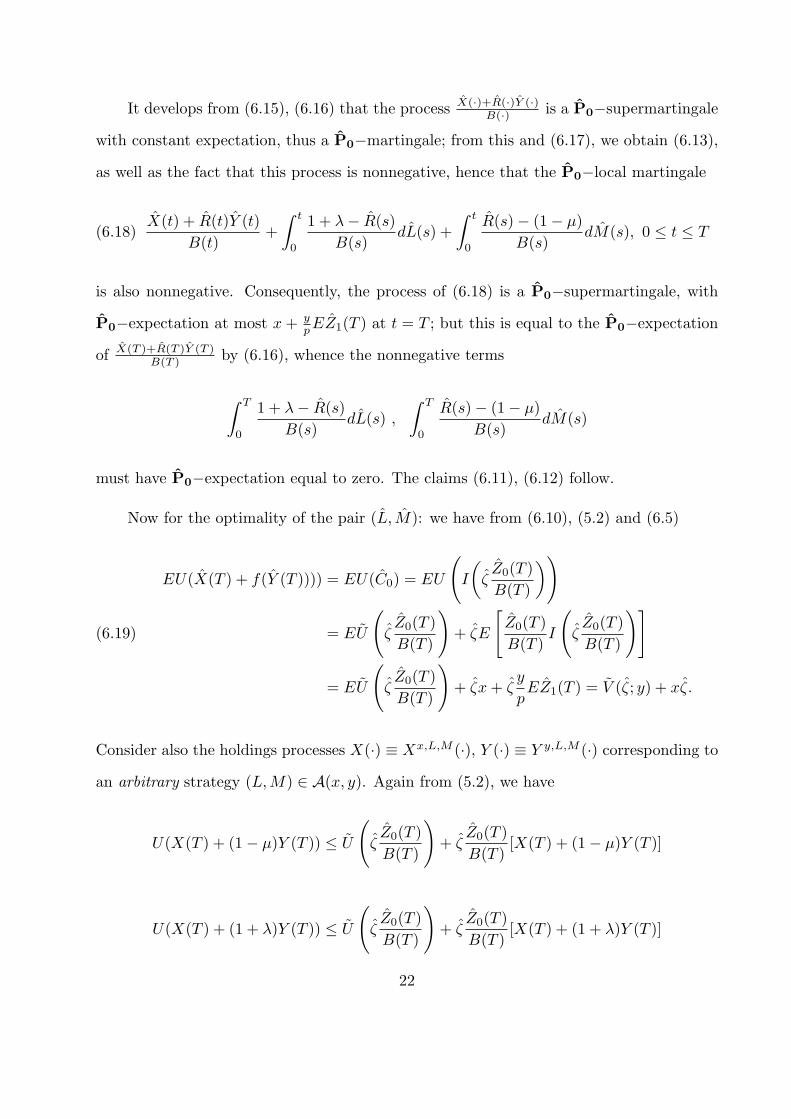
It develops from (6.15), (6.16) that the process X(·)+R(·)Y (·)B(·) is a P0−supermartingale

with constant expectation, thus a P0−martingale; from this and (6.17), we obtain (6.13),

as well as the fact that this process is nonnegative, hence that the P0−local martingale

(6.18)X(t) + R(t)Y (t)

B(t)+

∫ t

0

1 + λ− R(s)B(s)

dL(s) +∫ t

0

R(s)− (1− µ)B(s)

dM(s), 0 ≤ t ≤ T

is also nonnegative. Consequently, the process of (6.18) is a P0−supermartingale, with

P0−expectation at most x + ypEZ1(T ) at t = T ; but this is equal to the P0−expectation

of X(T )+R(T )Y (T )B(T ) by (6.16), whence the nonnegative terms

∫ T

0

1 + λ− R(s)B(s)

dL(s) ,

∫ T

0

R(s)− (1− µ)B(s)

dM(s)

must have P0−expectation equal to zero. The claims (6.11), (6.12) follow.

Now for the optimality of the pair (L, M): we have from (6.10), (5.2) and (6.5)

(6.19)

EU(X(T ) + f(Y (T )))) = EU(C0) = EU

(I

(ζZ0(T )B(T )

))

= EU

(ζZ0(T )B(T )

)+ ζE

[Z0(T )B(T )

I

(ζZ0(T )B(T )

)]

= EU

(ζZ0(T )B(T )

)+ ζx + ζ

y

pEZ1(T ) = V (ζ; y) + xζ.

Consider also the holdings processes X(·) ≡ Xx,L,M (·), Y (·) ≡ Y y,L,M (·) corresponding to

an arbitrary strategy (L,M) ∈ A(x, y). Again from (5.2), we have

U(X(T ) + (1− µ)Y (T )) ≤ U

(ζZ0(T )B(T )

)+ ζ

Z0(T )B(T )

[X(T ) + (1− µ)Y (T )]

U(X(T ) + (1 + λ)Y (T )) ≤ U

(ζZ0(T )B(T )

)+ ζ

Z0(T )B(T )

[X(T ) + (1 + λ)Y (T )]

22

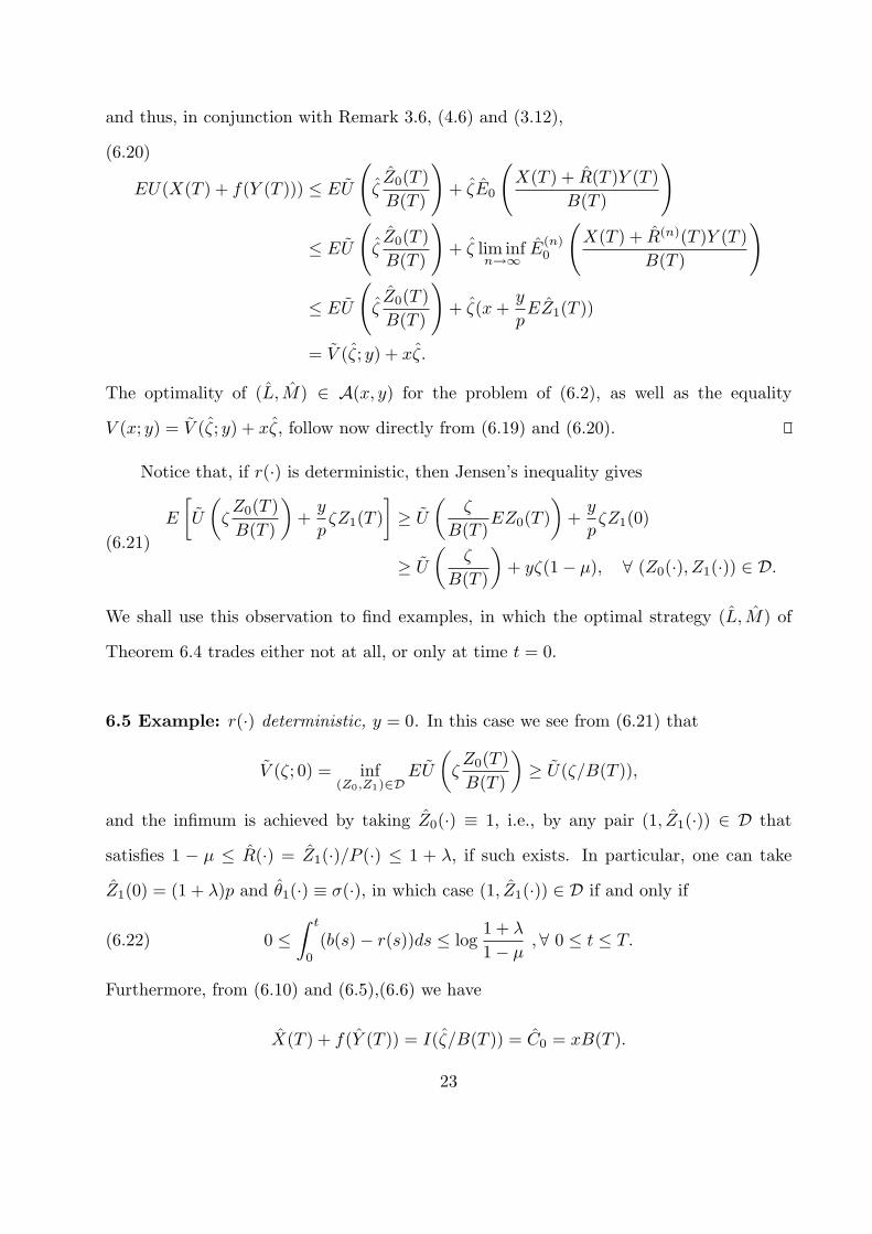
and thus, in conjunction with Remark 3.6, (4.6) and (3.12),

(6.20)

EU(X(T ) + f(Y (T ))) ≤ EU

(ζZ0(T )B(T )

)+ ζE0

(X(T ) + R(T )Y (T )

B(T )

)

≤ EU

(ζZ0(T )B(T )

)+ ζ lim inf

n→∞E

(n)0

(X(T ) + R(n)(T )Y (T )

B(T )

)

≤ EU

(ζZ0(T )B(T )

)+ ζ(x +

y

pEZ1(T ))

= V (ζ; y) + xζ.

The optimality of (L, M) ∈ A(x, y) for the problem of (6.2), as well as the equality

V (x; y) = V (ζ; y) + xζ, follow now directly from (6.19) and (6.20).

Notice that, if r(·) is deterministic, then Jensen’s inequality gives

(6.21)E

[U

(ζZ0(T )B(T )

)+

y

pζZ1(T )

]≥ U

(ζ

B(T )EZ0(T )

)+

y

pζZ1(0)

≥ U

(ζ

B(T )

)+ yζ(1− µ), ∀ (Z0(·), Z1(·)) ∈ D.

We shall use this observation to find examples, in which the optimal strategy (L, M) of

Theorem 6.4 trades either not at all, or only at time t = 0.

6.5 Example: r(·) deterministic, y = 0. In this case we see from (6.21) that

V (ζ; 0) = inf(Z0,Z1)∈D

EU

(ζZ0(T )B(T )

)≥ U(ζ/B(T )),

and the infimum is achieved by taking Z0(·) ≡ 1, i.e., by any pair (1, Z1(·)) ∈ D that

satisfies 1 − µ ≤ R(·) = Z1(·)/P (·) ≤ 1 + λ, if such exists. In particular, one can take

Z1(0) = (1 + λ)p and θ1(·) ≡ σ(·), in which case (1, Z1(·)) ∈ D if and only if

(6.22) 0 ≤∫ t

0

(b(s)− r(s))ds ≤ log1 + λ

1− µ, ∀ 0 ≤ t ≤ T.

Furthermore, from (6.10) and (6.5),(6.6) we have

X(T ) + f(Y (T )) = I(ζ/B(T )) = C0 = xB(T ).

23

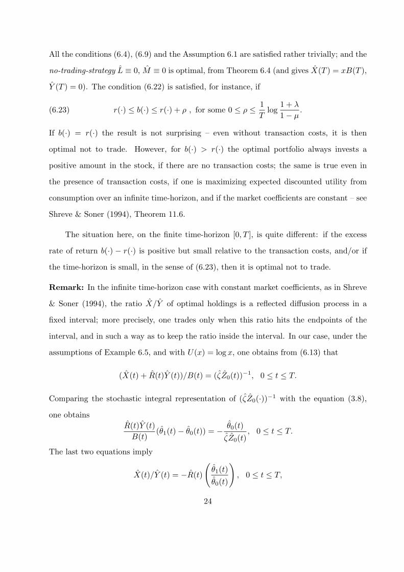
All the conditions (6.4), (6.9) and the Assumption 6.1 are satisfied rather trivially; and the

no-trading-strategy L ≡ 0, M ≡ 0 is optimal, from Theorem 6.4 (and gives X(T ) = xB(T ),

Y (T ) = 0). The condition (6.22) is satisfied, for instance, if

(6.23) r(·) ≤ b(·) ≤ r(·) + ρ , for some 0 ≤ ρ ≤ 1T

log1 + λ

1− µ.

If b(·) = r(·) the result is not surprising – even without transaction costs, it is then

optimal not to trade. However, for b(·) > r(·) the optimal portfolio always invests a

positive amount in the stock, if there are no transaction costs; the same is true even in

the presence of transaction costs, if one is maximizing expected discounted utility from

consumption over an infinite time-horizon, and if the market coefficients are constant – see

Shreve & Soner (1994), Theorem 11.6.

The situation here, on the finite time-horizon [0, T ], is quite different: if the excess

rate of return b(·) − r(·) is positive but small relative to the transaction costs, and/or if

the time-horizon is small, in the sense of (6.23), then it is optimal not to trade.

Remark: In the infinite time-horizon case with constant market coefficients, as in Shreve

& Soner (1994), the ratio X/Y of optimal holdings is a reflected diffusion process in a

fixed interval; more precisely, one trades only when this ratio hits the endpoints of the

interval, and in such a way as to keep the ratio inside the interval. In our case, under the

assumptions of Example 6.5, and with U(x) = log x, one obtains from (6.13) that

(X(t) + R(t)Y (t))/B(t) = (ζZ0(t))−1, 0 ≤ t ≤ T.

Comparing the stochastic integral representation of (ζZ0(·))−1 with the equation (3.8),

one obtainsR(t)Y (t)

B(t)(θ1(t)− θ0(t)) = − θ0(t)

ζZ0(t), 0 ≤ t ≤ T.

The last two equations imply

X(t)/Y (t) = −R(t)

(θ1(t)

θ0(t)

), 0 ≤ t ≤ T,

24

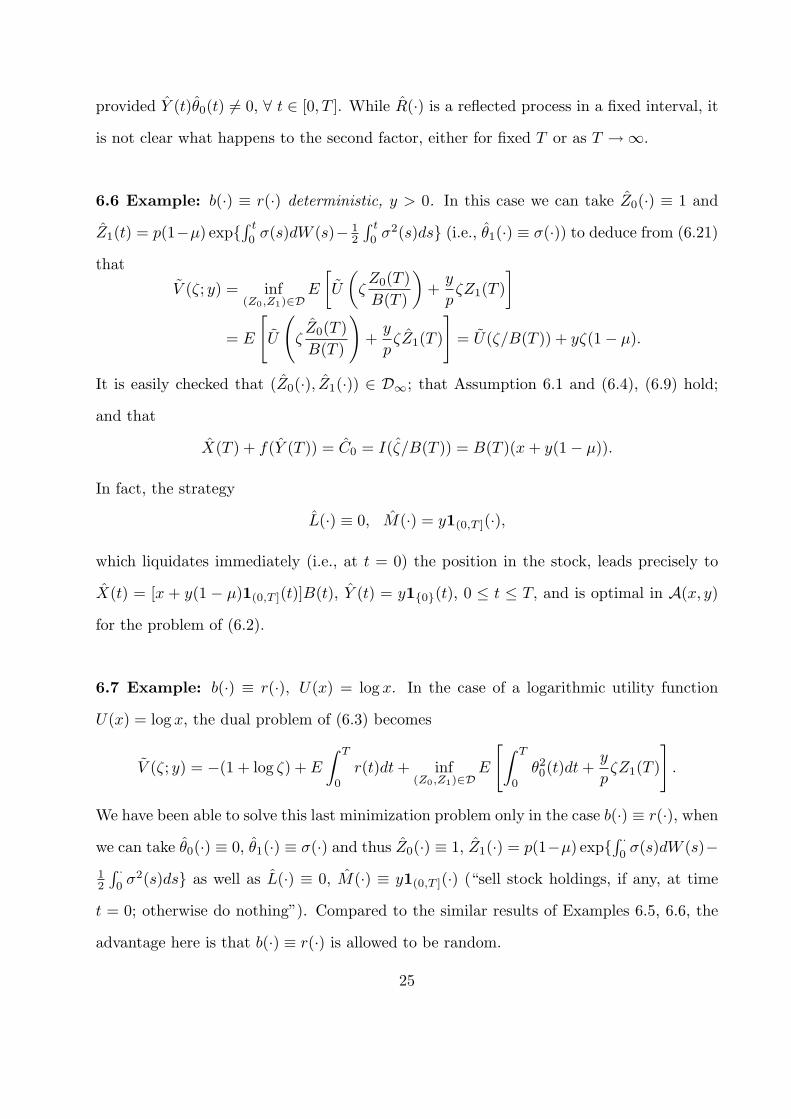
provided Y (t)θ0(t) 6= 0, ∀ t ∈ [0, T ]. While R(·) is a reflected process in a fixed interval, it

is not clear what happens to the second factor, either for fixed T or as T →∞.

6.6 Example: b(·) ≡ r(·) deterministic, y > 0. In this case we can take Z0(·) ≡ 1 and

Z1(t) = p(1−µ) exp∫ t

0σ(s)dW (s)− 1

2

∫ t

0σ2(s)ds (i.e., θ1(·) ≡ σ(·)) to deduce from (6.21)

that

V (ζ; y) = inf(Z0,Z1)∈D

E

[U

(ζZ0(T )B(T )

)+

y

pζZ1(T )

]

= E

[U

(ζZ0(T )B(T )

)+

y

pζZ1(T )

]= U(ζ/B(T )) + yζ(1− µ).

It is easily checked that (Z0(·), Z1(·)) ∈ D∞; that Assumption 6.1 and (6.4), (6.9) hold;

and that

X(T ) + f(Y (T )) = C0 = I(ζ/B(T )) = B(T )(x + y(1− µ)).

In fact, the strategy

L(·) ≡ 0, M(·) = y1(0,T ](·),

which liquidates immediately (i.e., at t = 0) the position in the stock, leads precisely to

X(t) = [x + y(1 − µ)1(0,T ](t)]B(t), Y (t) = y10(t), 0 ≤ t ≤ T, and is optimal in A(x, y)

for the problem of (6.2).

6.7 Example: b(·) ≡ r(·), U(x) = log x. In the case of a logarithmic utility function

U(x) = log x, the dual problem of (6.3) becomes

V (ζ; y) = −(1 + log ζ) + E

∫ T

0

r(t)dt + inf(Z0,Z1)∈D

E

[∫ T

0

θ20(t)dt +

y

pζZ1(T )

].

We have been able to solve this last minimization problem only in the case b(·) ≡ r(·), when

we can take θ0(·) ≡ 0, θ1(·) ≡ σ(·) and thus Z0(·) ≡ 1, Z1(·) = p(1−µ) exp∫ ·0σ(s)dW (s)−

12

∫ ·0σ2(s)ds as well as L(·) ≡ 0, M(·) ≡ y1(0,T ](·) (“sell stock holdings, if any, at time

t = 0; otherwise do nothing”). Compared to the similar results of Examples 6.5, 6.6, the

advantage here is that b(·) ≡ r(·) is allowed to be random.

25

Proof of Lemma 6.3: For simplicity of notation, we shall take again p = 1 and prove,

for any given ζ ∈ (0,∞) and (Z0(·), Z1(·)) ∈ D:

(6.24) E

[Z0(T )B(T )

I

(ζZ0(T )B(T )

)− yZ1(T )

]≤ E

[Z0(T )B(T )

I

(ζZ0(T )B(T )

)− yZ1(T )

]< ∞.

¿From condition (5.4) we have ηI(η) ≤ a+(1− b)U(I(η)), 0 < η < ∞, and by subtracting

(1− b)ηI(η) from both sides:

bηI(η) ≤ a + (1− b)U(η).

It follows that

bζE

[Z0(T )B(T )

I

(ζZ0(T )B(T )

)− yZ1(T )

]≤ a + (1− b)EU

(ζZ0(T )B(T )

)− byζZ1(0)

≤ a + (1− b)[V (ζ; y)− ζy(1− µ)

]− bζy(1− µ) < ∞,

which proves the second inequality in (6.24).

To prove the first inequality, we use a perturbation argument: for fixed but arbitrary

0 < ε < 1 and (Z0(·), Z1(·)) ∈ D, let

Z(ε)i (·) := (1− ε)Zi(·) + εZi(·), i = 0, 1

and note that (Z(ε)0 (·), Z(ε)

1 (·)) ∈ D. Because the pair (Z0(·), Z1(·)) ∈ D attains the

infimum in (6.3), we have E(G(ε)) ≤ 0, where

(6.25)

G(ε) :=1ε

[U

(ζZ0(T )B(T )

)− U

(ζZ

(ε)0 (T )B(T )

)]+

ζy

ε(Z1(T )− Z

(ε)1 (T ))

=ζ

B(T )I

(ζFε

B(T )

)(Z0(T )− Z0(T )) + ζy(Z1(T )− Z1(T ))

≥ ζ

B(T )I

(ζZ0(T )B(T )

)(Z0(T )− Z0(T )) + ζy(Z1(T )− Z1(T ))

≥ − ζ

B(T )Z0(T )I

(ζZ0(T )B(T )

)+ ζy(Z1(T )− Z1(T )),

where Fε is a random variable with values between Z0(T ) and Z(ε)0 (T ); in particular,

limε↓0 Fε = Z0(T ).

26

Suppose first that Z0(·)/Z∗0 (·) ≥ K for some constant 0 < K < ∞. Then, by Assump-

tion 6.1,

(6.26) E

[Z0(T )B(T )

I

(ζZ0(T )B(T )

)]≤ E

[Z0(T )B(T )

I

(ζKZ∗0 (T )

B(T )

)]< ∞,

so that the last random variable in (6.25) is integrable. Then from Fatou’s lemma, we have

(6.27)

E

[ζ

B(T )I

(ζZ0(T )B(T )

)(Z0(T )− Z0(T )) + ζy(Z1(T )− Z1(T ))

]

= E

[limε↓0

ζ

B(T )I

(ζFε

B(T )

)(Z0(T )− Z0(T )) + ζy(Z1(T )− Z1(T ))

]

≤ lim infε↓0

E(G(ε)) ≤ 0 ;

the inequality (6.24) follows.

Now for an arbitrary (Z0(·), Z1(·)) ∈ D, define τn := inft ∈ [0, T ]/Z0(t)/Z∗0 (t) ≤1n ∧ T . Proceed as in the proof of Lemma 4.1, to obtain a sequence (Z(n)

0 (·), Z(n)1 (·)) ∈

D such that Z(n)0 (·)/Z∗0 (·) ≥ 1/n. Therefore, the first inequality in (6.24) is valid for

(Z(n)0 (T ), Z(n)

1 (T )), ∀ n ∈ N, and we can let n →∞ and use Fatou’s lemma to obtain the

result for (Z0(T ), Z1(T )).

27

7. PRICING CONTINGENT CLAIMS.

We indicate here a possible way of pricing contingent claims in a market with transaction

costs. The minimal hedging price is only an upper bound for the price of a claim, and is

typically too high (see Example 4.3). Given a utility function U(·) and initial wealth x,

Davis (1994) defines the fair price of a claim in a market with frictions to be the price

which makes the agent’s utility neutral with respect to a small (infinitesimal) diversion of

funds into the claim (if such exists). See Davis (1994) and Karatzas & Kou (1994) for the

precise mathematical formulations. Assuming y = 0, it can be argued, using the methods

of those papers, that the fair price V (0) of a claim C = (C0, C1) in our setting should be

the expected value of the discounted claim evaluated under the optimal shadow state-price

densities of the dual problem, i.e., by

V (0) = E

[Z0(T )

C0

B(T )+ Z1(T )

C1

S(T )

],

provided that the dual optimization problem of (6.3) has a unique solution (Z0(·), Z1(·)).Notice that this price does not depend on the initial holdings x in stock, if the solution to

the dual problem does not depend on ζ, as in Assumption 6.1. However, V (0) does depend

in general on the return rate of the stock b(·). For example, if b(·) ≡ r(·) and deterministic,

and the claim is a European call, then it follows from Example 6.6 that the fair price is the

Black-Scholes price, independently of the utility function U(·) that is being considered. If

b(·) − r(·) is nonnegative and small, the price would be close to the Black-Scholes price.

Constantinides (1993) and Constantinides & Zariphopoulou (1995) show that the price of

a European call, under not too large transaction costs, is always close to the Black-Scholes

price. However, they use a different definition of (bounds for) the fair price, based on

maximizing utility from consumption plus utility from terminal wealth, adjusted for the

value of the claim at time t = T .

28

A. APPENDIX.

The purpose of this section is to prove the closedness property (4.14), for the set A0 of

(4.10), using a method similar to the one in the appendix of Shreve, Soner & Cvitanic

(1995). To this effect, let us consider a sequence (Un, Vn)n∈N ⊂ A0 converging in (L∗2)2

to some (U, V ) ∈ (L∗2)2, i.e.,

(A.1) E∗0 [(Un − U)2 + (Vn − V )2] −→ 0, as n →∞,

and observe that, as a result, the expected values E∗0 (U2

n), E∗0 (V 2

n ) are bounded uniformly

in n. Let also (Ln, Mn)n∈N ⊂ A(0, 0) denote the corresponding hedging strategies, so

that with Xn(·), Yn(·) defined by

(A.2)Xn(t) = −(1 + λ)Ln(t) + (1− µ)Mn(t) , 0 ≤ t ≤ T

Yn(t) = Ln(t)−Mn(t) +∫ t

0

σ(u)Yn(u)dW ∗0 (u), 0 ≤ t ≤ T

we have the following hedging and admissibility properties, for every n ∈ N:

(A.3)

Xn(T ) + (1− µ)Yn(T ) ≥ Un + (1− µ)Vn

Xn(T ) + (1 + λ)Yn(T ) ≥ Un + (1 + λ)Vn

,

(A.4) Qn(·) := Xn(·) + R(·)Yn(·) is a P0 − supermartingale, ∀ (Z0(·), Z1(·)) ∈ D∞.

The question then is, whether we can find (L,M) ∈ A(0, 0), so that (Ln,Mn) →(L,M) and (Xn, Yn) → (X, Y ) ≡ (X0,L,M , Y 0,L,M ), in a suitable sense, as n → ∞, and

still have the analogues of (A.3) and (A.4):

(A.5)

X(T ) + (1− µ)Y (T ) ≥ U + (1− µ)VX(T ) + (1 + λ)Y (T ) ≥ U + (1 + λ)V

,

(A.6) Q(·) := X(·) + R(·)Y (·) is a P0 − supermartingale, ∀ (Z0(·), Z1(·)) ∈ D∞.

29

Let us start by introducing some notation:

(A.7)

In(t) :=∫ t

0

σ(u)Yn(u)dW ∗0 (u)

Sλn(t) := E∗

0 [Un + (1 + λ)Vn|F(t)]

Sµn(t) := E∗

0 [Un + (1− µ)Vn|F(t)],

for 0 ≤ t ≤ T , and by noticing the inequalities (proved below):

(A.8) Sλn(t) ≤ Xn(t) + (1 + λ)Yn(t), Sµ

n(t) ≤ Xn(t) + (1− µ)Yn(t), 0 ≤ t ≤ T

(A.9) (λ+µ)Ln(t) ≤ (1−µ)In(t)−Sµn(t), (λ+µ)Mn(t) ≤ (1+λ)In(t)−Sλ

n(t), 0 ≤ t ≤ T

(A.10) |Yn(t)| ≤ 1 + λ

λ + µ|In(t)|+ |Sµ

n(t)|+ |Sλn(t)|

λ + µ, 0 ≤ t ≤ T

(A.11) sup0≤t≤T,n∈N

E∗0

[(Sλ

n(t))2 + (Sµn(t))2 + I2

n(t)]

=: C < ∞.

¿From (A.8)-(A.11) it develops that the sequences Ln(·)n∈N, Mn(·)n∈N, Xn(·)n∈N

and Yn(·)n∈N are bounded inH, the Hilbert space of progressively measurable, real-valued

processes ξ(t), 0 ≤ t ≤ T with E∗0

∫ T

0ξ2(t)dt < ∞ and < η, ξ >= E∗

0

∫ T

0η(t)ξ(t)dt. Thus,

there exist processes L(·),M(·) and Y (·) in H, such that

(A.12) Ln(·) → L(·), Mn(·) → M(·), Yn(·) → Y (·) weakly in H, as n →∞

(possibly only along a subsequence, which is then relabelled). We can define then

(A.13) X(·) := (1− µ)M(·)− (1 + λ)L(·), and notice that Xn(·) → X(·) weakly in H.

¿From Lemmata 4.5-4.7 in Karatzas & Shreve (1984), we can assume that L(·),M(·)have increasing, left-continuous paths, and that

(A.14)

Ln(t) → L(t), Mn(t) → M(t) as n →∞weakly in L1(Ω,F(T ),P∗0), for a.e. t ∈ [0, T ].

30

It follows from (A.14) that, for every h ∈ (0, T ), we have

limn→∞

E∗0 (Ln(T )1A) ≥ 1

hlim

n→∞

∫ T

T−h

E∗0 (Ln(s)1A)ds =

1h

∫ T

T−h

E∗0 (L(s)1A)ds ≥ E∗

0 (L(T−h)1A),

and letting h ↓ 0:

(A.15) limn→∞

E∗0 (Ln(T )1A) ≥ E∗

0 (L(T )1A), ∀ A ∈ F(T ).

Similarly,

(A.16) limn→∞

E∗0 (Mn(T )1A) ≥ E∗

0 (M(T )1A), ∀ A ∈ F(T ).

Recall now the definition (A.7) of In(·) and define the process

(A.17) I(t) :=∫ t

0

σ(s)Y (s)dW ∗0 (s), 0 ≤ t ≤ T.

We can show (see below) that

(A.18) In(t) → I(t) as n →∞ weakly in L∗2, ∀ t ∈ [0, T ].

It develops then, by taking weak limits in (A.2), that the processes X(·), Y (·) of (A.13),

(A.12) satisfy

X(t) = −(1 + λ)L(t) + (1− µ)M(t) , 0 ≤ t ≤ T

Y (t) = L(t)−M(t) +∫ t

0

σ(u)Y (u)dW ∗0 (u), 0 ≤ t ≤ T.

(This is verified first for fixed t ∈ [0, T ], and then for all 0 ≤ t ≤ T simultaneously by the

left-continuity of the processes involved.) In other words,

X(·) ≡ X0,L,M (·) and Y (·) ≡ Y 0,L,M (·).

To finish the argument it remains to verify the properties (A.5) and (A.6) of hedging and

admissibility, respectively.

31

PROOF OF (A.5): Hedging. In view of (A.2), we may write (A.3) as

(1− µ)In(T )− (λ + µ)Ln(T ) ≥ Un + (1− µ)Vn

(1 + λ)In(T )− (λ + µ)Mn(T ) ≥ Un + (1 + λ)Vn;

We want to deduce from this (A.5), or equivalently

(A.19) (1− µ)I(T )− (λ + µ)L(T ) ≥ U + (1− µ)V

(A.20) (1 + λ)I(T )− (λ + µ)M(T ) ≥ U + (1 + λ)V.

Recall from (A.16), (A.18), (A.1) that

(λ + µ)E∗0 [M(T )1A] ≤ (λ + µ) lim

n→∞E∗

0 [Mn(T )1A]

≤ limn→∞

E∗0

[(1 + λ)(In(T )− Vn)− Un1A

]

= E∗0

[(1 + λ)(I(T )− V )− U1A

], ∀ A ∈ F(T )

and (A.20) follows; a similar argument gives (A.19).

PROOF OF (A.6): Admissibility. Fix an arbitrary (Z0(·), Z1(·)) in D∞; from (A.3)

and Remark 3.6 we have Qn(T ) := Xn(T ) + R(T )Yn(T ) ≥ Un + R(T )Vn, and (A.4) gives

then

(A.21) Qn(t) ≥ E0[Qn(T )|F(t)] ≥ E0[Un + R(T )Vn|F(t)] ≥ −ξn(t), 0 ≤ t ≤ T.

Here

(A.22) ξn(t) := E0[|Un|+(1+λ)|Vn| |F(t)], ξ(t) := E0[|U |+(1+λ)|V | |F(t)], 0 ≤ t ≤ T

are P0−martingales, with continuous paths and

(A.23) sup0≤t≤T,n∈N

E0[ξ2n(t) + ξ2(t)] < ∞, E0[ max

0≤t≤T|ξn(t)− ξ(t)|]2 −→

n→∞0.

Indeed,

E0ξ2n(t) ≤ E0ξ

2n(T ) ≤ 2KE∗

0 [U2n + (1 + λ)2V 2

n ] ≤ KCλ < ∞,

32

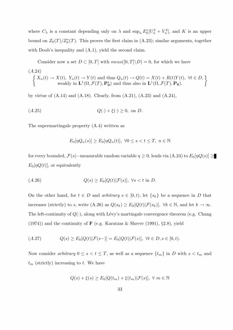
where Cλ is a constant depending only on λ and supn E∗0 [U2

n + V 2n ], and K is an upper

bound on Z0(T )/Z∗0 (T ). This proves the first claim in (A.23); similar arguments, together

with Doob’s inequality and (A.1), yield the second claim.

Consider now a set D ⊂ [0, T ] with meas([0, T ]\D) = 0, for which we have

(A.24)Xn(t) → X(t), Yn(t) → Y (t) and thus Qn(t) → Q(t) = X(t) + R(t)Y (t), ∀t ∈ D,

weakly in L1(Ω,F(T ),P∗0) and thus also in L1(Ω,F(T ),P0).

by virtue of (A.14) and (A.18). Clearly, from (A.21), (A.23) and (A.24),

(A.25) Q(·) + ξ(·) ≥ 0, on D.

The supermartingale property (A.4) written as

E0[ηQn(s)] ≥ E0[ηQn(t)], ∀0 ≤ s < t ≤ T, n ∈ N

for every bounded, F(s)−measurable random variable η ≥ 0, leads via (A.24) to E0[ηQ(s)] ≥E0[ηQ(t)], or equivalently

(A.26) Q(s) ≥ E0[Q(t)|F(s)], ∀s < t in D.

On the other hand, for t ∈ D and arbitrary s ∈ [0, t), let sk be a sequence in D that

increases (strictly) to s, write (A.26) as Q(sk) ≥ E0[Q(t)|F(sk)], ∀k ∈ N, and let k →∞.

The left-continuity of Q(·), along with Levy’s martingale convergence theorem (e.g. Chung

(1974)) and the continuity of F (e.g. Karatzas & Shreve (1991), §2.8), yield

(A.27) Q(s) ≥ E0[Q(t)|F(s−)] = E0[Q(t)|F(s)], ∀t ∈ D, s ∈ [0, t).

Now consider arbitrary 0 ≤ s < t ≤ T , as well as a sequence tm in D with s < tm and

tm (strictly) increasing to t. We have

Q(s) + ξ(s) ≥ E0[Q(tm) + ξ(tm)|F(s)], ∀ m ∈ N

33

from (A.27) and the martingale property of ξ(·); recall (A.25) and let m →∞ to conclude,

from Fatou’s lemma, the continuity of ξ(·) and the left-continuity of Q(·), that

E0[Q(t)|F(s)] + ξ(s) = E0[Q(t) + ξ(t)|F(s)] = E0[limm

(Q(tm) + ξ(tm))|F(s)]

≤ lim infm

E0[Q(tm) + ξ(tm)|F(s)] ≤ Q(s) + ξ(s), ∀ 0 ≤ s < t ≤ T,

which establishes (A.6). The proof of the closedness property (4.14) is now complete.

Proof of (A.8): ¿From (A.7), (A.3), (A.4) and Remark 3.1 with z = 1 + λ, we have

R∗(·) ≡ 1+λ, Sλn(t) ≤ E∗

0 [Xn(T )+(1+λ)Yn(T )|F(t)] = E∗0 [Xn(T )+R∗(T )Yn(T )|F(t)] ≤

Xn(t)+R∗(t)Yn(t) = Xn(t)+(1+λ)Yn(t), first for fixed t and then, by continuity of Sλn(·)

and left-continuity of Xn(·), Yn(·), for all t ∈ [0, T ] simultaneously. Similarly for Sµn(·) (but

with z = 1− µ in Remark 3.1).

Proof of (A.9), (A.10): From (A.2) and (A.8), we obtain (A.9), as well as

Yn(t) ≤ In(t) + Ln(t) ≤ 1 + λ

λ + µIn(t)− Sµ

n(t)λ + µ

Yn(t) ≥ In(t)−Mn(t) ≥ − 1− µ

λ + µIn(t) +

Sλn(t)

λ + µ,

which lead to (A.10).

Proof of (A.11): For Sλn(·), Sµ

n(·) we have in fact the stonger property

(A.28) supτ∈S,n∈N

E∗0 [(Sλ

n(τ)2 + (Sµn(τ))2] ≤ 2 sup

n∈NE∗

0 [U2n + (1 + λ)V 2

n ] ≤ K < ∞

from Jensen’s inequality and (A.7), (A.1), where S is the class of stopping times of F with

values in [0, T ]. For fixed n ∈ N, k ∈ N, t ∈ [0, T ], define

τ (k)n := infs ∈ [0, t]/|Yn(s)| ≥ k ∧ t; Y (k)

n (s) := Yn(s) if s ≤ τ (k)n , Y (k)

n (s) = 0 if s > τ (k)n

I(k)n (s) := In(s ∧ τ (k)

n ) =∫ s

0

σ(u)Y (k)n (u)dW ∗

0 (u), 0 ≤ s ≤ t.

34

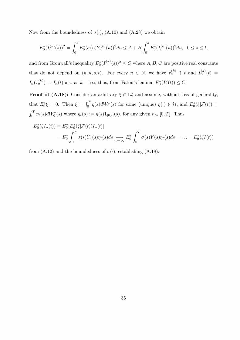
Now from the boundedness of σ(·), (A.10) and (A.28) we obtain

E∗0 (I(k)

n (s))2 =∫ s

0

E∗0 (σ(u)Y (k)

n (u))2du ≤ A + B

∫ s

0

E∗0 (I(k)

n (u))2du, 0 ≤ s ≤ t,

and from Gronwall’s inequality E∗0 (I(k)

n (s))2 ≤ C where A,B, C are positive real constants

that do not depend on (k, n, s, t). For every n ∈ N, we have τ(k)n ↑ t and I

(k)n (t) =

In(τ (k)n ) → In(t) a.s. as k →∞; thus, from Fatou’s lemma, E∗

0 (I2n(t)) ≤ C.

Proof of (A.18): Consider an arbitrary ξ ∈ L∗2 and assume, without loss of generality,

that E∗0ξ = 0. Then ξ =

∫ T

0η(s)dW ∗

0 (s) for some (unique) η(·) ∈ H, and E∗0 (ξ|F(t)) =

∫ T

0ηt(s)dW ∗

0 (s) where ηt(s) := η(s)1[0,t](s), for any given t ∈ [0, T ]. Thus

E∗0 (ξIn(t)) = E∗

0 [E∗0 (ξ|F(t))In(t)]

= E∗0

∫ T

0

σ(s)Yn(s)ηt(s)ds −→n→∞

E∗0

∫ T

0

σ(s)Y (s)ηt(s)ds = . . . = E∗0 (ξI(t))

from (A.12) and the boundedness of σ(·), establishing (A.18).

35

B. APPENDIX.

We establish in this section the existence of an optimal pair (L, M) ∈ A+(x, y) for the

expected utility maximization problem of (6.2):

(B.1) V (x; y) = EU(Xx,L,M (T ) + f(Y y,L.M (T ))) < ∞.

For simplicity of notation, we shall take again p = 1 and r(·) ≡ 0. The key idea is to

consider the set

(B.2) Ax,y := H ∈ L∗2 / ∃(L,M) ∈ A+(x, y) that hedges (H, 0)

of “terminal bank account holdings hedgeable by admissible strategies”, and to show that

(B.3) Ax,y is a convex, closed and bounded subset of L∗2.

These properties can be established by using the methodology of Appendix A, almost line-

by-line (with very few, and obvious, changes), so we leave the details to the care of the

diligent reader. Let us denote

(B.4) J(H) := −EU(H), H ∈ L∗2;

we will show that the value function of (6.2) can be re-written as

(B.5) −V (x; y) = infH∈Ax,y

J(H),

and that the infimum in (B.5) is attained (and thus is the supremum in (6.2)).

It is clear that the functional

(B.6) J : L∗2 −→ R ∪ +∞

defined by (B.4) is convex; let us verify that it is also proper (as indicated in (B.6)), i.e.,

that

(B.7) EU(H) < ∞, ∀ H ∈ L∗2.

36

Indeed, the function U(·) is sublinear: U(x) ≤ a + bx, ∀ 0 ≤ x < ∞ for some a > 0, b > 0.

Thus EU(H) ≤ const.(1 + E|H|) < ∞, since E∗0 (H2) < ∞, because

E|H| = E∗0

[|H| exp

−

∫ T

0

θ∗0(s)dW (s) +12

∫ T

0

|θ∗0(s)|2ds

]

= E∗0

[|H| exp

−

∫ T

0

θ∗0(s)dW ∗0 (s)− 1

2

∫ T

0

|θ∗0(s)|2ds

]

≤(

E∗0 (H2)E∗

0

[exp

−

∫ T

0

2θ∗0(s)dW ∗0 (s)− 1

2

∫ T

0

|2θ∗0(s)|2ds

exp

∫ T

0

|θ∗0(s)|2ds

]) 12

≤ (E∗

0 (H2)) 1

2 e12 k2T < ∞,

where k is an upper bound on |θ∗0(·)| of (3.6), Remark 3.1.

Finally, the functional J of (B.4), (B.6) is lower-semicontinuous in the topology of L∗2;

indeed, if Hnn∈N converges to H in the topology of L∗2, we have

(B.8) limn→∞

E|Hn −H| = 0.

Thus, from Fatou’s lemma, E[a + bH −U(H)] ≤ lim infn→∞E[a + bHn −U(Hn)], and we

obtain the lower-semicontinuity property J(H) ≤ lim infn→∞ J(Hn) in conjunction with

(B.8), (B.4).

To recapitulate: in (B.5), we are minimizing the convex, proper, lower-semicontinuous

functional J , over the closed, convex and bounded subset Ax,y of L∗2. From a basic result of

convex analysis (e.g. Ekeland & Temam (1976), p. 35) the functional J attains its infimum

over Ax,y, at a point H of Ax,y. Now (H, 0) is hedged by some pair (L, M) ∈ A+(x, y)

(recall (B.2)) with corresponding terminal holdings (X(T ), Y (T )), which implies

(B.9) G := X(T ) + f(Y (T )) = H.

Indeed, if this were not the case, we would have G ≥ H a.s., and G > H with positive

probability, because of the hedging property of Definition 2.1; moreover, since (L, M) obvi-

ously hedges (G, 0), this would contradict the optimality of H and the strict monotonicity

37

of U(·), provided that G ∈ L∗2 – but this follows from the remarks preceding the proof of

Theorem 4.2, since G ≥ 0 and (X(T ), Y (T )) hedges (G, 0).

It is now clear from (B.9) and the optimality of H that (L, M) is optimal for the

problem of (6.2), and that (B.5) holds; in particular, V (x, y) = −EU(H) < ∞.

Acknowledgements. We are grateful to S. Kusuoka and A. Cadenillas for sending us

preprints of their papers, as well as to S. Shreve for useful comments and suggestions.

REFERENCES

AVELLANEDA, M. & PARAS, A. (1994) Dynamic hedging portfolios for derivative se-curities in the presence of large transaction costs. Applied Mathematical Finance 1,165-194.

BENSAID, B., LESNE, J., PAGES, H. & SCHEINKMAN, J. (1992) Derivative assetpricing with transaction costs. Mathematical Finance 2 (2), 63 -86.

BLACK, F. & SCHOLES, M. (1973) The pricing of options and corporate liabilities.J. Polit. Economy 81, 637-659.

BOYLE, P. P. & TAN, K. S. (1994) Lure of the linear. Risk 7/4, 43-46.BOYLE, P. P. & VORST, T. (1992) Option replication in discrete time with transaction

costs. J. Finance 47, 272-293.CADENILLAS, A. & HAUSSMAN, U.G. (1993) The consumption investment problem

with transaction costs and random coefficients. Private communication.CADENILLAS, A. & HAUSSMAN, U.G. (1994) The stochastic maximum principle for a

singular control problem. Stochastics 49, 211-238.CHUNG, K. L. (1974) A Course in Probability Theory (Second Edition). Academic Press,

New York.CONSTANTINIDES, G. M. (1993) Option pricing bounds with transaction costs. Preprint,

Graduate School of Business, University of Chicago.CONSTANTINIDES, G. M., & ZARIPHOPOULOU, T. (1995) Universal bounds on option

prices with proportional transaction costs. Preprint.CUOCO, D. (1994) Optimal policies and equilibrium prices with portfolio cone constraints

and stochastic labor income. Preprint, The Wharton School, University of Pennsyl-vania.

CVITANIC, J. & KARATZAS, I. (1992) Convex duality in constrained portfolio optimiza-tion. Ann. Appl. Probab. 2, 767-818.

CVITANIC, J. & KARATZAS, I. (1993) Hedging contingent claims with constrained port-

38

folios. Ann. Appl. Probab. 3, 652-681.DAVIS, M.H.A. (1994) A general option pricing formula. Preprint, Imperial College,

London.DAVIS, M. H .A. & CLARK, J. M. C. (1994) A note on super-replicating strategies. Phil.

Trans. Royal Soc. London A 347, 485-494.DAVIS, M. H. A. & NORMAN, A. (1990) Portfolio selection with transaction costs. Math.

Operations Research 15, 676-713.DAVIS, M. H. A. & PANAS, V. G. (1994) The writing price of a European contingent

claim under proportional transaction costs. Comp. Appl. Math. 13, 115-157.DAVIS, M. H. A., PANAS, V. G. & ZARIPHOPOULOU, T. (1993) European option

pricing with transaction costs. SIAM J. Control & Optimization 31, 470-493.DAVIS, M. H. A. & ZARIPHOPOULOU, T. (1995) American options and transaction

fees. In Mathematical Finance, M. H. A. Davis et al. ed., The IMA Volumes inMathematics and its Applications 65, 47-62. Springer-Verlag.

DEWYNNE, J. N., WHALLEY, A. E. & WILMOTT, P. (1993) Path-dependent options.Phil. Trans. Royal Soc. London A 347, 517-529.

EDIRISINGHE, C., NAIK, V. & UPPAL, R. (1993) Optimal replication of options withtransaction costs and trading restrictions. J. Financial & Quantitative Analysis 28,117-138.

EKELAND, I. & TEMAM, R. (1976) Convex Analysis and Variational Problems. North-Holland, Amsterdam and Elsevier, New York.

FIGLEWSKI, S. (1989) Options arbitrage in imperfect markets, J. Finance 44, 1289–1311.FLESAKER, B. & HUGHSTON, L. P. (1994) Contingent claim replication in continuous

time with transaction costs. Proc. Derivative Securities Conference, Cornell Univer-sity.

GILSTER, J. E. & LEE, W. (1984) The effect of transaction costs and different borrowingand lending rates on the option pricing model. J. Finance 43, 1215-1221.

HARRISON, J. M. & KREPS, D. M. (1979) Martingales and arbitrage in multiperiodsecurity markets. J. Econom. Theory 20, 381–408.

HARRISON, J. M. & PLISKA, S. R. (1981) Martingales and stochastic integrals in thetheory of continuous trading. Stochastic Processes and Appl. 11, 215–260.

HARRISON, J. M. & PLISKA, S. R. (1983) A stochastic calculus model of continuoustime trading: complete markets. Stochastic Processes and Appl. 15, 313–316.

HENROTTE, P. (1993) Transaction costs and duplication strategies. Groupe HEC, DepartementFinance et Economie, preprint.

HODGES, S. D. & CLEWLOW, L. J. (1993), Optimal delta-hedging under transactioncosts. Financial Options Research Center preprint, University of Warwick.

HODGES, S.D. & NEUBERGER, A. (1989) Optimal replication of contingent claims undertransaction costs. Review of Future Markets 8, 222-239.

HOGGARD, T., WHALLEY, A.E., & WILMOTT, P. (1994) Hedging option portfolios inthe presence of transaction costs. Adv. in Futures and Options Research, 7, 21-35.

JOUINI, E. & KALLAL, H. (1991) Martingales, arbitrage and equilibrium in securitiesmarkets with transaction costs. Preprint, Laboratoire d’Econometrie, Ecole Polytech-

39

nique.KARATZAS, I. (1989) Optimization problems in the theory of continuous trading. SIAM

J. Control & Optimization 27, 1221-1259.KARATZAS, I. & KOU, S-G. (1994) On the pricing of contingent claims under constraints.

Preprint, Columbia University.KARATZAS, I. & SHREVE, S.E. (1984) Connections between optimal stopping and singu-

lar stochastic control I. Monotone follower problems. SIAM J. Control & Optimization22, 856-877.

KARATZAS, I. & SHREVE, S.E. (1991) Brownian Motion and Stochastic Calculus (2nd

edition), Springer-Verlag, New York.KUSUOKA, S. (1995) Limit theorem on option replication with transaction costs. Ann.

Appl. Probab. 5, 198-221.LELAND, H.E. (1985) Option pricing and replication with transaction costs. J. Finance

40, 1283-1301.LEVENTAL, S. & SKOROHOD, A. V. (1995) On the possibility of hedging options in the

presence of transactions costs. Preprint, Michigan State University.MAGILL, M.J.P. & CONSTANTINIDES, G.M. (1976) Portfolio selection with transaction

costs. J. Economic Theory 13, 264-271.MERTON, R.C. (1973) Theory of rational option pricing. Bell J. Econ. Manag. Sci. 4,

141-183.MERTON, R. C. (1989) On the application of the continuous time theory of finance to

financial intermediation and insurance, The Geneva Papers on Risk and Insurance,225–261.

MEYER, P. A. (1976) Un cours sur les integrales stochastiques. Lecture Notes in Math-ematics 511, 245-398. Sem. Probabilites X, Univ. de Strasbourg. Springer-Verlag,New York.

MORTON, A. J. & PLISKA, S. R. (1993) Optimal portfolio management with fixed trans-action costs, Math. Finance, to appear.

PANAS, V. G. (1993) Option pricing with transaction costs. Doctoral Dissertation, Impe-rial College, London.

PLISKA, S. R. & SELBY, M. J. P. (1993) On a free boundary problem that arises inportfolio management, Dept. of Finance, University of Illinois at Chicago, preprint.

PROTTER, P. (1990) Stochastic Integration and Differential Equations. Springer-Verlag,New York.

SHEN, Q. (1990) Bid-ask prices for call options with transaction costs, Working paper,The Wharton School, University of Pennsylvania.

SHIRAKAWA, H. & KONNO, H. (1995) Pricing of options under the proportional trans-action costs. Department of Industrial and Systems Engineering, Tokyo Institute ofTechnology. Preprint.

SHREVE, S. E. & SONER, H. M. (1994) Optimal investment and consumption withtransaction costs, Ann. Appl. Probab. 4, 609-692.

SONER, H. M., SHREVE, S. E. & CVITANIC, J. (1995) There is no nontrivial hedgingportfolio for option pricing with transaction costs, Ann. Appl. Probab. 5, 327-355.

40

TAKSAR, M., KLASS, M.J. & ASSAF, D. (1988) A diffusion model for optimal portfolioselection in the presence of brokerage fees, Math. Operations Research 13, 277-294.

TOFT, K. B. (1993) Exact formulas for expected hedging error and transactions costs inoption replication, University of California at Berkeley, preprint.

Department of Statistics Department of StatisticsColumbia University Columbia UniversityNew York, NY 10027 New York, NY 10027cj@stat.columbia.edu ik@stat.columbia.eduTel. (212)854-3652 Tel. (212)854-3652

41