Hardware/Software Partitioning Greg Stitt ECE Department University of Florida

Hardware/Software Partitioning

Greg StittECE Department

University of Florida

Introduction

FPGAs are often much faster than sw But, most real designs with FPGAs still use

microprocessors Why?

FPGAs typically implement “kernels” efficiently Difficult/inefficient to implement entire

application as a custom circuit in FPGA Common case

Implement performance critical code in FPGA Implement everything else on

microprocessors Certain regions can afford to be slow

Hw/Sw Architectures

Hybrids/ASIPs Tensilica Xtensa is uP with custom instructions in hw Stretch is similar with FPGA Piperench, Warp processors, Chameleon, etc.

FPGAs FPGAs more commonly have microprocessor cores in

fabric Virtex II Pro, Virtex IV FX have PowerPCs

Even if no uP cores in fabric, can implement uP on FPGA - soft core uPs

Microblaze, Picoblaze, Nios Slow, but sometimes not a problem

High-Performance Computing Cray XD1 - AMDs/FPGAs SGI Altix - Xeons/FPGAs


Definition: Given an application, hw/sw partitioning maps each region of the application onto hardware (custom circuits) or software (microprocessors)

A partition is a mapping of each region to either hw or sw Possible Goals

Meet design constraints (performance, power, size, cost, etc.)

Maximize performance Minimize power for a given performance constraint Etc.

Challenges Huge number of partitions for an application

# of partitions = 2n, n is number of regions 5 regions = 32 partitions, 100 regions = 1.26*1030 partitions!

Clearly, we need efficient heuristics


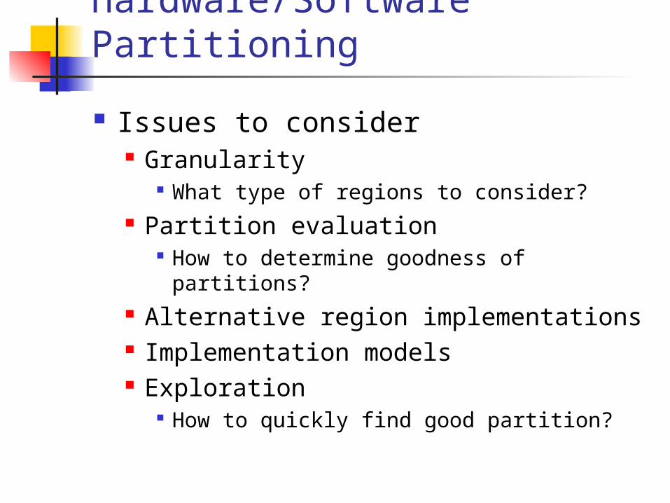
Issues to consider Granularity

What type of regions to consider? Partition evaluation

How to determine goodness of partitions? Alternative region implementations Implementation models Exploration

How to quickly find good partition?

Granularity

Definition: Measure of functionality considered for hw/sw

Coarse grained regions - tasks, functions, loops Fine grained regions - blocks, statements, operations

Tradeoffs exist for coarse grained/fine grained Coarse grained regions

Simplifies partitioning (fewer regions) Possibly more accurate estimations (don’t have to combine a

bunch of small regions) Possibly less inter-partition communication

Hw/Sw communication usually expensive May outweigh benefits of putting regions in hardware

Fine grained regions May take longer to find good partition (more partitions to

choose from) Estimation possibly more difficult But, may provide better solution

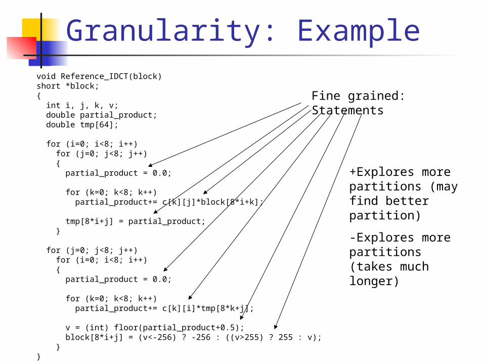
Granularity: Examplevoid Reference_IDCT(block)short *block;{ int i, j, k, v; double partial_product; double tmp[64];

for (i=0; i<8; i++) for (j=0; j<8; j++) { partial_product = 0.0;

for (k=0; k<8; k++) partial_product+= c[k][j]*block[8*i+k];

tmp[8*i+j] = partial_product; }

for (j=0; j<8; j++) for (i=0; i<8; i++) { partial_product = 0.0;

for (k=0; k<8; k++) partial_product+= c[k][i]*tmp[8*k+j];

v = (int) floor(partial_product+0.5); block[8*i+j] = (v<-256) ? -256 : ((v>255) ? 255 : v); }}

Coarse grained: Functions and loops

+Few regions

+Easier estimation (less hw/sw communication)

-May not provide optimal partition (explores less possibilities)








Fine grained: Statements

+Explores more partitions (may find better partition)

-Explores more partitions (takes much longer)








Very fine grained: Individual Operations

+Most flexible (allows exploration of all possibilities)

-Huge number of regions

Etc.

Partition Evaluation

Responsible for determining the “goodness” of a partition

Evaluates multiple design metrics Performance, power, area, etc. May use some cost function for

representing goodness e.g. weighted average of multiple metrics

HWSWPerformance – 28.5sArea – 62000 gatesPower - 2 watts

Loop1Loop2

Quantize()

DCT()Huffman()


Input: Partition

Output: Design Metrics


Complicated problem Regions are not independent

e.g. adding more regions to hw may seem to improve performance but may require more steering logic, clock may be lengthened, etc.

Must consider effects of regions on each other Must consider many architectural issues

e.g. Communication time for hw-hw, hw-sw, sw-sw May be different for each architectural component

E.g. heterogeneous microprocessors

2 possibilities for evaluation Implementation - actually implement each partition,

determine design metrics Accurate, but slow

Estimation Estimation - less accurate/faster

Partition Evaluation: Implementation/Estimation

Evaluation techniques - many others Pure implementation

Possible only for a small number of regions Pure estimation

Likely inaccurate Hybrid approach 1

Implement hardware/software for individual regions (ignore possible combinations)

Characterize regions with performance/area Estimate changes when combining regions

Hybrid approach 2 Iterate by estimating goodness of partitions, with occasional

implementations to verify estimates Hybrid approach 3

Estimate some good partitions to reduce exploration space, implement those few partitions, choose best one

Hybrid approach 4 Combine estimation and implementation.

E.g. use “rough” synthesis to get hardware performance

Alternative Region Implementations

10s15s25s 10s

5s

12s

8s 5s

Sw Time: 50s Sw Time: 30s Sw Time: 20s

Application Regions(Different sized shapes represent different hw implementations)

FIR() ACCUM()

SEARCH()

5s25s

10s10s 15s

Possible Solutions: Use fastest implementations

Use smallest implementations

Consider all “middle” implementations

5+30+20=55s 25+15+10=50s 10+15+20=45sPerformance:Best Partition

15s

Alternative Region Implementations

Issue: Hw regions can be implemented in many ways Challenge 1: How to choose an implementation for each

region? Making one region fast may make partition slow

May use area needed by other regions May need to choose slow implementation to save area for

other regions Must consider entire partition for each change to each

region Challenge 2: Exploration space explodes!

For 8 regions w/ 1 hw implementation, possible partitions = 28 = 256

For 8 regions w/ 4 hw implementations, possible partitions = 58 = 390625 partitions!

5 possible implementations for each region = 1 sw + 4 hw Good solution: unknown

Implementation Models Implementation models define how microprocessors

interface with hardware More possibilities, better solutions, but larger solution

space Estimation techniques more difficult for complex models

Example 1: Communication methods Direct communication, using shared memory, tightly-

coupled, etc.

Microprocessor

Cache

DMA

Bridge

Memory

Tightly-coupled

Loosely-coupled

Fused

Directcommunication

Dynamically reconfigurable

Implementation Models

Example 2: Execution models Mutually exclusive

FPGA and uP never execute simultaneously May be appropriate for sequential applications

Advantage: easier estimations Disadvantage: decreased performance

Parallel Advantage: Improved performance Disadvantage: Estimates much more

difficult Must take into account memory contention,

cache coherency, synchronization, etc.

Exploration

Exploration searches partition space for a optimal partition - realistically must settle for good partition

Main step: represents majority of hw/sw partitioning work

Highly dependent on formulation of problems A formulation is a particular instance of discussed

issues e.x. direct communication, sequential regions, 1

implementation per region, etc. HWSWHWSW

Performance – 28.5sArea – 1452 gates

HWSW



HWSW


Exploration

Simple formulation: n regions, each region has Sw time, Hw time, and Hw area

Assumptions Adding hw regions together doesn’t change

area/performance Obviously not true But, may be good enough in some situations

Communication time of regions same for Hw or Sw

Often not true, but may be true if uP and Hw has same interface to memory

Exploration

A solution for simple formulation: Problem identical to 0-1 knapsack problem

NP-complete 0-1 knapsack problem

Input: knapsack with weight capacity, and a set of items with profit and weight

Problem: Determine which items should be placed in the knapsack

Goal: maximizing profit without violating weight capacity Mapping to hw/sw partitioning

Knapsack is hw (FPGA in our case) Weight capacity is hw area Items are program regions Profit is speedup from implementation in hw Weight is area of hw implemention

Exploration: Heuristics for simple formulation

Problem: 0-1 knapsack is NP-complete We likely need to use a heuristic Need way of focusing on moving

regions to hw that provide large speedup

How do we know if a region potentially provides large speedup?


Amdahl’s Law Originally stated how much performance could be improved

by parallelization Can be generalized to stating how much speedup is achieved

based on the percentage of the application that is optimized Speedup = 1/(s-p/n)

p is percentage of app. that is optimized, s is the percentage unoptimized (1-p), n is the speedup of the region created by the optimization

Ideal Speedup = 1/(s) = 1/(1-p) Speedup assuming that hw runs infinitely fast

From these equations, we can see that heuristics should focus on regions consisting of a large % of execution time

The larger p is for a region, the larger the potential speedup is

p = 90%, ideal speedup = 1/(1-.9) = 10x p = 10%, ideal speedup = 1/(1-.1) = 1.1x


90-10 rule Observation that for many applications 90% of

execution time spent in 10% of code

Good news for heuristic Suggests heuristic can achieve most of potential speedup

by focusing on moving this 10% of code to hardware

0%

20%

40%

60%

80%

100%

1 2 3 4 5 6 7 8 9 10

Most-frequent regions

Cumulative application execution percentage


Possible greedy heuristic 1) Profile application to determine % of execution time for

each region Part of input for simple formulation

2) Create speedup/area ratio for regions with largest % Partition evaluation - may be estimate or implementation How many regions?

Depends on how fast you want heuristic to be 3) Sort regions based on this ratio 4) Implement regions in sorted order until area exhausted O(n lgn) complexity

Mapping back to knapsack problem Basic idea: Place items in knapsack in order of

profit/weight

Exploration More complicated formulations

More complex implementation models Asymmetric communication Multiple processors Multiple FPGAs Tightly-coupled vs loosely coupled Multiple implementations Etc.

Common exploration techniques: ILP Simulated annealing/genetic algorithms/hill climbing Group migration (Kernighan-Lin) Graph bipartitioning (read paper on website) Tabu search (read paper on website)

Similar to simulated annealing, but maintains “Tabu” list to improve diversity of solutions

Exploration There is no known efficient solution for considering all

possible issues Ridiculously large exploration space Problem is becoming harder with more complex architectures

State of the art: Granularity

Consider coarse and fine grained partitions Partition evaluation

Estimation and “rough” implementation Alternative region implementations

Typically only consider a single implementation of each region Area for future improvements - a lot of interesting problems

How to decide how many implementations to consider? How to decide which implementations to consider?

Implementation models Typically assume architectures with few options

One type of communication, no dynamic reconfiguration, etc. Future architectures will increase options

Should improve partition, but increase exploration space

Summary

Applications often not efficient in pure hw Hw/sw partitioning maps regions of application

onto sw (microprocessors) and hw (custom circuit)

Goal: Maximize performance, meet design constraints, etc.

Issues Granularity of regions Partition evaluation Alternative region implementations Implementation models Exploration techniques

Focus of most work

Documents

Hardware/Software Partitioning Greg Stitt ECE Department University of Florida