Embed Size (px)
Citation preview

Hardware DesignBased on Verilog HDL
Gordon J. PaceBalliol College
Oxford University Computing Laboratory
Programming Research Group
Trinity Term 1998
Thesis submitted for the degree of Doctor of Philosophy
at the University of Oxford

Abstract
Up to a few years ago, the approaches taken to check whether a hardware com-ponent works as expected could be classified under one of two styles: hardwareengineers in the industry would tend to exclusively use simulation to (empiri-cally) test their circuits, whereas computer scientists would tend to advocate anapproach based almost exclusively on formal verification. This thesis proposesa unified approach to hardware design in which both simulation and formalverification can co-exist.
Relational Duration Calculus (an extension of Duration Calculus) is devel-oped and used to define the formal semantics of Verilog HDL (a standard indus-try hardware description language). Relational Duration Calculus is a temporallogic which can deal with certain issues raised by the behaviour of typical hard-ware description languages and which are hard to describe in a pure temporallogic. These semantics are then used to unify the simulation of Verilog pro-grams, formal verification and the use of algebraic laws during the design stage.A simple operational semantics based on the simulation cycle is shown to beisomorphic to the denotational semantics. A number of laws which programssatisfy are also given, and can be used for the comparison of syntactically dif-ferent programs.
The thesis also presents a number of other results. The use of a temporallogic to specify the semantics of the language makes the development of pro-grams which satisfy real-time properties relatively easy. This is shown in a casestudy. The fuzzy boundary in interpreting Verilog programs as either hardwareor software is also exploited by developing a compilation procedure to translateprograms into hardware. Hence, the two extreme interpretations of hardwaredescription languages as software, with sequential composition as the topmostoperator (as in simulation), and as hardware with parallel composition as thetopmost operator are exposed.
The results achieved are not limited to Verilog. The approach taken wascarefully chosen so as to be applicable to other standard hardware descriptionlanguages such as VHDL.

All of a sudden, it occurred to me that I
could try again in a different way, more sim-
ple and rapid, with guaranteed success. I be-
gan making patterns again, correcting them,
complicating them. Again I was trapped in
this quicksand, locked in this maniacal ob-
session. Some nights I woke up and ran to
note a decisive correction, which then led to
an endless series of shifts. On other nights I
would go to bed relieved at having found the
perfect formula; and the next morning, on
waking, I would tear it up. Even now, with
the book in the galleys, I continue to work
over it, take it apart, rewrite. I hope that
when the volume is printed I will be outside
it once and for all. But will this ever hap-
pen?
The Castle of Crossed Destinies
Italo Calvino, 1969

Acknowledgements
First of all, I would like to thank my supervisor, Jifeng He, for frequent andfruitful discussions about the work presented in this thesis. I would also like tothank all those in Oxford with similar research interests, discussions with whomregularly led to new and interesting ideas.
Thanks also go all my colleagues at the Department of Computer Science andArtificial Intelligence at the University of Malta, especially Juanito Camilleri,for providing a wonderful working environment during this past year.
Needless to say, I would like to thank all my friends, too numerous to list,who helped to make the years I spent in Oxford an unforgettable period of mylife. Also, thanks go to my parents whose constant support can never be fullyacknowledged.
Finally, but certainly not least, thanks go to Sarah, for encouragement,dedication and patience, not to mention the long hours she spent proof-readingthis thesis.
I also wish to acknowledge the financial help of the Rhodes Trust, whopartially supported my studies in Oxford.

Contents
1 Introduction 11.1 Aims and Motivation . . . . . . . . . . . . . . . . . . . . . . . . . 1
1.1.1 Background . . . . . . . . . . . . . . . . . . . . . . . . . . 11.1.2 Broad Aims . . . . . . . . . . . . . . . . . . . . . . . . . 21.1.3 Achievements . . . . . . . . . . . . . . . . . . . . . . . . . 31.1.4 Overview of Existent Research . . . . . . . . . . . . . . . 41.1.5 Choosing an HDL . . . . . . . . . . . . . . . . . . . . . . 51.1.6 Verilog or VHDL? . . . . . . . . . . . . . . . . . . . . . . 6
1.2 Details of the Approach Taken . . . . . . . . . . . . . . . . . . . 71.2.1 General Considerations . . . . . . . . . . . . . . . . . . . 71.2.2 Temporal Logic . . . . . . . . . . . . . . . . . . . . . . . . 7
1.3 Overview of Subsequent Chapters . . . . . . . . . . . . . . . . . . 8
I 10
2 Verilog 112.1 Introduction . . . . . . . . . . . . . . . . . . . . . . . . . . . . . . 11
2.1.1 An Overview . . . . . . . . . . . . . . . . . . . . . . . . . 112.2 Program Structure . . . . . . . . . . . . . . . . . . . . . . . . . . 122.3 Signal Values . . . . . . . . . . . . . . . . . . . . . . . . . . . . . 132.4 Language Constructs . . . . . . . . . . . . . . . . . . . . . . . . . 13
2.4.1 Programs . . . . . . . . . . . . . . . . . . . . . . . . . . . 142.4.2 Example Programs . . . . . . . . . . . . . . . . . . . . . 17
2.5 The Simulation Cycle . . . . . . . . . . . . . . . . . . . . . . . . 172.5.1 Initialisation . . . . . . . . . . . . . . . . . . . . . . . . . 182.5.2 Top-Level Modules . . . . . . . . . . . . . . . . . . . . . . 19
2.6 Concluding Comments . . . . . . . . . . . . . . . . . . . . . . . . 20
3 Relational Duration Calculus 213.1 Introduction . . . . . . . . . . . . . . . . . . . . . . . . . . . . . . 213.2 Duration Calculus . . . . . . . . . . . . . . . . . . . . . . . . . . 21
3.2.1 The Syntax . . . . . . . . . . . . . . . . . . . . . . . . . . 213.2.2 Lifting Predicate Calculus Operators . . . . . . . . . . . . 223.2.3 The Semantics . . . . . . . . . . . . . . . . . . . . . . . . 233.2.4 Validity . . . . . . . . . . . . . . . . . . . . . . . . . . . . 253.2.5 Syntactic Sugaring . . . . . . . . . . . . . . . . . . . . . . 26
3.3 Least Fixed Point . . . . . . . . . . . . . . . . . . . . . . . . . . . 273.3.1 Open Formulae . . . . . . . . . . . . . . . . . . . . . . . . 273.3.2 Fixed Points . . . . . . . . . . . . . . . . . . . . . . . . . 273.3.3 Monotonicity . . . . . . . . . . . . . . . . . . . . . . . . . 283.3.4 Semantics of Recursion . . . . . . . . . . . . . . . . . . . 28
i

3.4 Discrete Duration Calculus . . . . . . . . . . . . . . . . . . . . . 293.5 Relational Duration Calculus . . . . . . . . . . . . . . . . . . . . 29
3.5.1 Introduction . . . . . . . . . . . . . . . . . . . . . . . . . 293.5.2 The Syntax and Informal Semantics . . . . . . . . . . . . 303.5.3 The Semantics . . . . . . . . . . . . . . . . . . . . . . . . 31
3.6 Laws of the Relational Chop Operator . . . . . . . . . . . . . . . 343.7 Conclusions . . . . . . . . . . . . . . . . . . . . . . . . . . . . . . 35
4 Real Time Specifications 374.1 The Real Time Operators . . . . . . . . . . . . . . . . . . . . . . 37
4.1.1 Invariant . . . . . . . . . . . . . . . . . . . . . . . . . . . 374.1.2 Followed By . . . . . . . . . . . . . . . . . . . . . . . . . . 384.1.3 Leads To . . . . . . . . . . . . . . . . . . . . . . . . . . . 384.1.4 Unless . . . . . . . . . . . . . . . . . . . . . . . . . . . . . 394.1.5 Stability . . . . . . . . . . . . . . . . . . . . . . . . . . . . 40
4.2 Discrete Duration Calculus . . . . . . . . . . . . . . . . . . . . . 404.3 Summary . . . . . . . . . . . . . . . . . . . . . . . . . . . . . . . 40
II 41
5 Formal Semantics of Verilog 425.1 Introduction . . . . . . . . . . . . . . . . . . . . . . . . . . . . . . 425.2 Syntax and Informal Semantics of Verilog . . . . . . . . . . . . . 425.3 The Formal Semantics . . . . . . . . . . . . . . . . . . . . . . . . 46
5.3.1 The Techniques Used . . . . . . . . . . . . . . . . . . . . 465.3.2 Syntactic Equivalences . . . . . . . . . . . . . . . . . . . . 475.3.3 The Primitive Instructions . . . . . . . . . . . . . . . . . 475.3.4 Constructive Operators . . . . . . . . . . . . . . . . . . . 505.3.5 Top-Level Instructions . . . . . . . . . . . . . . . . . . . . 52
5.4 Other Extensions to the Language . . . . . . . . . . . . . . . . . 535.4.1 Local Variables . . . . . . . . . . . . . . . . . . . . . . . . 535.4.2 Variable Initialisation . . . . . . . . . . . . . . . . . . . . 535.4.3 Delayed Continuous Assignments . . . . . . . . . . . . . . 545.4.4 Transport Delay . . . . . . . . . . . . . . . . . . . . . . . 545.4.5 Non-Blocking Assignments . . . . . . . . . . . . . . . . . 55
5.5 Discussion . . . . . . . . . . . . . . . . . . . . . . . . . . . . . . . 575.5.1 Avoiding Combinational Loops . . . . . . . . . . . . . . . 575.5.2 Time Consuming Programs . . . . . . . . . . . . . . . . . 575.5.3 Extending Boolean Types . . . . . . . . . . . . . . . . . . 585.5.4 Concurrent Read and Write . . . . . . . . . . . . . . . . . 59
5.6 Related Work . . . . . . . . . . . . . . . . . . . . . . . . . . . . . 595.7 Conclusions . . . . . . . . . . . . . . . . . . . . . . . . . . . . . . 60
6 Algebraic Laws 616.1 Introduction . . . . . . . . . . . . . . . . . . . . . . . . . . . . . . 616.2 Notation . . . . . . . . . . . . . . . . . . . . . . . . . . . . . . . . 616.3 Monotonicity . . . . . . . . . . . . . . . . . . . . . . . . . . . . . 626.4 Assignment . . . . . . . . . . . . . . . . . . . . . . . . . . . . . . 656.5 Parallel and Sequential Composition . . . . . . . . . . . . . . . . 666.6 Non-determinism and Assumptions . . . . . . . . . . . . . . . . . 686.7 Conditional . . . . . . . . . . . . . . . . . . . . . . . . . . . . . . 696.8 Loops . . . . . . . . . . . . . . . . . . . . . . . . . . . . . . . . . 706.9 Continuous Assignments . . . . . . . . . . . . . . . . . . . . . . . 73
ii

6.10 Communication . . . . . . . . . . . . . . . . . . . . . . . . . . . . 746.11 Algebraic Laws for Communication . . . . . . . . . . . . . . . . . 74
6.11.1 Signal Output . . . . . . . . . . . . . . . . . . . . . . . . 746.11.2 Wait on Signal . . . . . . . . . . . . . . . . . . . . . . . . 756.11.3 Continuous Assignment Signals . . . . . . . . . . . . . . . 76
6.12 Signals and Merge . . . . . . . . . . . . . . . . . . . . . . . . . . 766.13 Conclusions . . . . . . . . . . . . . . . . . . . . . . . . . . . . . . 77
III 78
7 A Real Time Example 797.1 Introduction . . . . . . . . . . . . . . . . . . . . . . . . . . . . . . 797.2 System Specification . . . . . . . . . . . . . . . . . . . . . . . . . 79
7.2.1 The Boolean States Describing the System . . . . . . . . 797.2.2 System Requirements . . . . . . . . . . . . . . . . . . . . 807.2.3 System Assumptions . . . . . . . . . . . . . . . . . . . . . 81
7.3 Implementing the Specification . . . . . . . . . . . . . . . . . . . 827.4 Specification and Implementation Decomposition . . . . . . . . . 827.5 Calculation of the Implementation . . . . . . . . . . . . . . . . . 83
7.5.1 Closing and Opening the Gate . . . . . . . . . . . . . . . 837.5.2 The Traffic Lights . . . . . . . . . . . . . . . . . . . . . . 83
7.6 The Implementation . . . . . . . . . . . . . . . . . . . . . . . . . 857.7 Other Requirements . . . . . . . . . . . . . . . . . . . . . . . . . 85
8 Hardware Components 878.1 Combinational Circuits . . . . . . . . . . . . . . . . . . . . . . . 878.2 Transport Delay . . . . . . . . . . . . . . . . . . . . . . . . . . . 878.3 Inertial Delay . . . . . . . . . . . . . . . . . . . . . . . . . . . . . 878.4 Weak Inertial Delay . . . . . . . . . . . . . . . . . . . . . . . . . 888.5 Edge Triggered Devices . . . . . . . . . . . . . . . . . . . . . . . 888.6 Weak Edge Triggered Devices . . . . . . . . . . . . . . . . . . . . 888.7 Hiding . . . . . . . . . . . . . . . . . . . . . . . . . . . . . . . . . 898.8 Composition of Properties . . . . . . . . . . . . . . . . . . . . . 898.9 Algebraic Properties of Hardware Components . . . . . . . . . . 90
8.9.1 Combinational Properties . . . . . . . . . . . . . . . . . . 908.9.2 Delay Properties . . . . . . . . . . . . . . . . . . . . . . . 918.9.3 Edge Triggers . . . . . . . . . . . . . . . . . . . . . . . . . 928.9.4 Composition . . . . . . . . . . . . . . . . . . . . . . . . . 928.9.5 Hiding . . . . . . . . . . . . . . . . . . . . . . . . . . . . . 93
8.10 Reducing Properties to a Normal Form . . . . . . . . . . . . . . . 948.10.1 The Normal Form . . . . . . . . . . . . . . . . . . . . . . 948.10.2 Transport to Inertial Delay . . . . . . . . . . . . . . . . . 948.10.3 Weak Inertial Delays . . . . . . . . . . . . . . . . . . . . . 958.10.4 Edge Triggered Registers . . . . . . . . . . . . . . . . . . 95
8.11 Reduction to Normal Form . . . . . . . . . . . . . . . . . . . . . 968.12 Implementation of Properties in Verilog . . . . . . . . . . . . . . 978.13 Summary . . . . . . . . . . . . . . . . . . . . . . . . . . . . . . . 99
iii

9 Decomposition of Hardware Component Specifications: Exam-ples 1009.1 A Combinational n-bit Adder . . . . . . . . . . . . . . . . . . . . 100
9.1.1 Combinational Gates . . . . . . . . . . . . . . . . . . . . . 1019.1.2 Half Adder . . . . . . . . . . . . . . . . . . . . . . . . . . 1019.1.3 Full Adder . . . . . . . . . . . . . . . . . . . . . . . . . . 1029.1.4 Correctness of the Full Adder . . . . . . . . . . . . . . . . 1029.1.5 n-bit Adder . . . . . . . . . . . . . . . . . . . . . . . . . . 1039.1.6 Implementation in Verilog . . . . . . . . . . . . . . . . . . 105
9.2 Delayed Adder . . . . . . . . . . . . . . . . . . . . . . . . . . . . 1059.2.1 The Logic Gates . . . . . . . . . . . . . . . . . . . . . . . 1069.2.2 Half Adder . . . . . . . . . . . . . . . . . . . . . . . . . . 1069.2.3 Full Adder . . . . . . . . . . . . . . . . . . . . . . . . . . 1069.2.4 Proof of Correctness . . . . . . . . . . . . . . . . . . . . . 1079.2.5 n-bit Delayed Adder . . . . . . . . . . . . . . . . . . . . . 1089.2.6 Implementation in Verilog . . . . . . . . . . . . . . . . . . 108
9.3 Triggered Adder . . . . . . . . . . . . . . . . . . . . . . . . . . . 1099.3.1 Components . . . . . . . . . . . . . . . . . . . . . . . . . 1099.3.2 Decomposition of the Specification . . . . . . . . . . . . . 1099.3.3 Implementation . . . . . . . . . . . . . . . . . . . . . . . . 110
9.4 Conclusions . . . . . . . . . . . . . . . . . . . . . . . . . . . . . . 110
IV 112
10 A Hardware Compiler for Verilog 11310.1 Introduction . . . . . . . . . . . . . . . . . . . . . . . . . . . . . . 11310.2 Triggered Imperative Programs . . . . . . . . . . . . . . . . . . . 11410.3 The Main Results . . . . . . . . . . . . . . . . . . . . . . . . . . . 116
10.3.1 Sequential Composition . . . . . . . . . . . . . . . . . . . 11610.3.2 Conditional . . . . . . . . . . . . . . . . . . . . . . . . . . 11710.3.3 Loops . . . . . . . . . . . . . . . . . . . . . . . . . . . . . 118
10.4 Compilation . . . . . . . . . . . . . . . . . . . . . . . . . . . . . . 11910.5 Conclusions . . . . . . . . . . . . . . . . . . . . . . . . . . . . . . 124
10.5.1 Other Constructs . . . . . . . . . . . . . . . . . . . . . . . 12410.5.2 Basic Instructions . . . . . . . . . . . . . . . . . . . . . . 12510.5.3 Single Runs . . . . . . . . . . . . . . . . . . . . . . . . . . 12510.5.4 Overall Comments . . . . . . . . . . . . . . . . . . . . . . 126
11 An Operational Semantics of Verilog 12711.1 Introduction . . . . . . . . . . . . . . . . . . . . . . . . . . . . . . 12711.2 The Program Semantics . . . . . . . . . . . . . . . . . . . . . . . 128
11.2.1 Infinite Tail Programs . . . . . . . . . . . . . . . . . . . . 12811.2.2 Finite Loops . . . . . . . . . . . . . . . . . . . . . . . . . 128
11.3 The Operational Semantics . . . . . . . . . . . . . . . . . . . . . 12911.3.1 Immediate Transitions . . . . . . . . . . . . . . . . . . . 12911.3.2 Extension to Parallel Composition . . . . . . . . . . . . . 13111.3.3 Unit Time Transitions . . . . . . . . . . . . . . . . . . . . 132
11.4 Equivalence of Semantics . . . . . . . . . . . . . . . . . . . . . . 13611.4.1 An Informal Account . . . . . . . . . . . . . . . . . . . . . 13611.4.2 Formalising the Problem . . . . . . . . . . . . . . . . . . . 13611.4.3 Refinement Based on the Denotational Semantics . . . . . 13711.4.4 Refinement Based on the Operational Semantics . . . . . 13811.4.5 Preliminary Results . . . . . . . . . . . . . . . . . . . . . 139
iv

11.4.6 Unifying the Operational and Denotational Semantics . . 14211.5 Conclusions . . . . . . . . . . . . . . . . . . . . . . . . . . . . . . 145
V 146
12 Conclusions and Future Work 14712.1 An Overview . . . . . . . . . . . . . . . . . . . . . . . . . . . . . 14712.2 Shortcomings . . . . . . . . . . . . . . . . . . . . . . . . . . . . . 14712.3 Future Work . . . . . . . . . . . . . . . . . . . . . . . . . . . . . 148
12.3.1 Other Uses of Relational Duration Calculus . . . . . . . . 14812.3.2 Mechanised Proofs . . . . . . . . . . . . . . . . . . . . . . 14912.3.3 Real-Time Properties and HDLs . . . . . . . . . . . . . . 14912.3.4 Extending the Sub-Languages . . . . . . . . . . . . . . . . 149
12.4 Conclusion . . . . . . . . . . . . . . . . . . . . . . . . . . . . . . 150
Bibliography 151
v

Chapter 1
Introduction
1.1 Aims and Motivation
1.1.1 Background
System verification is one of the main raisons d’etre of computer science. Var-ious different approaches have been proposed and used to formally define thesemantics of computer languages, and one can safely say that most computerscientists have, at some point in their research, tackled this kind of problem orat least a similar one. One particular facet of this research is hardware veri-fication. Before discussing the possible role of computer science in hardware,it may be instructive to take a look at how hardware is usually developed inpractice.
In contrast to software, checking hardware products by building and then testingon a number of ‘typical’ inputs and comparing the outputs with the expectedresults, can be prohibitively expensive. Building a prototype circuit after everyiteration of the debugging process involves much more resources, ranging fromtime to money, than those involved in simply recompiling the modified sourcecode.
This gave rise to the concept of simulation of hardware using software. If hard-ware can be simulated by software efficiently and correctly, then the expenseof developing hardware can be reduced to that of software and, similarly, theorder of the speed of development of hardware can be pushed up to be on thesame level as that for software
This idea can be pushed further. Since the comparison of input and output pairscan be a tiresome and hence error prone process, given a description of a hard-ware product, one can build a shell around it to successively feed in a numberof inputs and compare them to the expected outputs. Hence, simply by givinga table of results, an engineer can design and use a testing module which wouldprotest if the given circuit failed any of the tests. This makes the debuggingprocess easier, and furthermore the results are more easily reproducible.
But certain devices can be described more easily than by giving a whole tableof input, output pairs. For some, a simple equation can suffice, while for othersit may be necessary to use an algorithm. Hence, if the simulator is also giventhe ability to parse algorithms, one can check circuits more easily. For example,given a circuit and a claim that it computes the nth Fibonacci number (wheren is the input), we can easily test the circuit for some inputs by comparingits output to the result of a short program evaluating Fibonacci numbers using
1

recursion or iteration. If the algorithmic portions in the simulator can be some-how combined with the hardware description parts, one can also start with analgorithmic ‘specification’ and gradually convert it into a circuit.
This is the main motivation behind the development and design of hardwaredescription languages. Basically, they provide a means of describing hardwarecomponents, extended with algorithmic capabilities, which can be efficientlysimulated in software to allow easy and cheap debugging facilities for hardware.
As in software, hardware description languages (henceforth HDLs) would benefitgreatly if research is directed towards formalising their semantics.
1.1.2 Broad Aims
In the hardware industry, simulation is all too frequently considered synony-mous with verification. The design process usually consists of developing animplementation from a specification, simulating both in software for a numberof different inputs and comparing the results. Bugs found are removed and theprocess repeated over and over again, until no new bugs are discovered. Thisprocedure, however, can only show the presence of errors, not their absence.
On the other hand, formal methods cannot replace existing methods of hardwaredesign overnight. Figure 1.1 proposes one possible framework via which formalmethods may be introduced in hardware design. The approach is completelybuilt upon formal techniques but includes simulation for design visualisation anddevelopment. Formal laws helping hardware engineers to correctly transformspecifications into the implementation language are also included. The resultis more reliability within an environment which does not require a completerevolution over current trends.
• Both the specification and implementation languages are formally definedwithin the same mathematical framework. This means that the statement:‘implementation I is a refinement of specification S’ is formally definedand can be checked to be (or not to be) the case beyond any reasonabledoubt.
• Design rules which transform a code portion from one format into anotherare used to help the designer transform a specification into a format moredirectly implementable as a hardware component. These rules are verifiedto be correct within the semantic domain, and hence the implementationis certain to be reliable.
• The relation between the simulator semantics and the semantics for theimplementation language can also be shown. By formally defining thesimulation cycle, we can check whether the semantics of a program asderived from the implementation language match the meaning which canbe inferred from the simulation of the program.
The synthesis process is effectively a compilation task, which can be verifiedto be correct — that the resultant product is equivalent to (or a refinementof) the original specification code. However, since the design rules may not becomplete, leaving situations unresolved, the inclusion of simulation within theformal model is used to help in the design process. This is obviously the areain which formal tools fit best. A verified hardware compiler which transformshigh level HDL code into a format which directly represents hardware is oneinstance of such a tool.
2

Simulation
simulation processFormally defined
Design RulesImplementation
to behavioural semanticsSimulation semantics equivalent
Formally verified algebraic laws Formal semantics forindustry standard HDLspecification language
Formal semantics for
Specification
Figure 1.1: Simulation and verification: a unified approach
Since the design procedure is not always decidable, it may leave issues open,which it hands over to the designer to resolve. The simulator may then be usedto remove obvious bugs, after which, it can be formally verified.
This is not the first time that a framework to combine simulation and formal ver-ification techniques has been proposed. Other approaches have been proposedelsewhere in the literature.
In view of these facts, a formal basis for an HDL is of immediate concern. As inthe case of software, one would expect that, in general, verifying large circuitswould still be a daunting task. However, it should hopefully be feasible to verifysmall sensitive sub-circuits. This indicates the importance of a compositionalapproach which allows the joining of different components without having torestart the verification process from scratch.
Finally, another important aim is to analyse the interaction between softwareand hardware. A circuit is usually specified by a fragment of code which mimicsthe change of state in the circuit. Since most HDLs include imperative languageconstructs, a study of this feature will help anyone using an HDL to consider thepossibility of implementing certain components in software. At the opposite endof the spectrum, software designers may one day include HDL-like constructs intheir software languages to allow them to include hardware components withintheir code.
The aim of this research is thus twofold:
1. To investigate the formal semantics of a hardware description language
2. To study possible algebraic methods and formal hardware techniques whichcan aid the process of verification and calculation of products. These tech-niques will ideally be of a general nature and the ideas they used wouldbe applicable to other HDLs.
1.1.3 Achievements
The original contributions presented in this thesis can be split into a number ofdifferent areas:
• At the most theoretical level, we present a variant of Duration Calculus,which can deal with certain situations which normal Duration Calculusfails to handle. Since the conception of Relational Duration Calculus, anumber of similar extensions to Duration Calculus have sprung up inde-pendently. Despite this we still believe that Relational Duration Calculus
3

can express certain constraints much more elegantly than similar calculi.A justification of this statement is given in chapter 3.
• Relational Duration Calculus is used to specify a semantics of a subsetof Verilog. We do not stop at giving the semantics to this subset, butinvestigate other Verilog instructions where the more complex semanticsexpose better the inherent assumptions made in the exposition of theinitially examined constructs.
• Algebraic laws allow straightforward syntactic reasoning about semanticcontent and are thus desirable. The semantics of Verilog are used to derivea suite of useful algebraic laws which allow comparison of syntacticallydifferent programs.
• The semantics are also used to transform specifications in different stylesinto Verilog programs. One of the two styles, real-time specifications, hasbeen, in our opinion, largely ignored in formal treatments of HDLs. Theother style shows how one can define a simple specification language andgive a decision procedure to transform such a specification into Verilogcode. Some examples are given to show how such a specification languagecan be used.
• Finally, the two opposing aspects in which one can view HDLs, as softwareor as hardware, is investigated in the last few chapters. On one hand,Verilog is simulated in software, essentially, by reducing it into a sequentialprogram. On the other hand, certain Verilog constructs have a directinterpretation as hardware.
– We start by showing that the denotational semantics of Verilog aresound and complete with respect to a simple version of Verilog sim-ulation cycle semantics (given as an operational semantics). Essen-tially, this allows us to transform Verilog programs into sequentialprograms.
– At the other end of the spectrum, we define, and prove correct, acompilation procedure from Verilog programs into a large collectionof simple programs running in parallel. Most of these programs canbe directly implemented in hardware.
This allows a projection of Verilog programs in either of the two differentdirections.
As can be deduced from this short summary, the main contribution of this thesisis to give a unified view of all these issues for Verilog HDL. Some of the aspectstreated in this thesis had previously been left unexplored with respect to HDLsin general.
In exploring these different viewpoints, we have thus realised a basis for theformal framework shown in figure 1.1 and discussed in the previous section.
1.1.4 Overview of Existent Research
Frameworks similar to the one proposed have been developed and researchedtime and time again for software languages. However, literature on the join-ing of the two, where hardware simulation and verification are put within thesame framework, is relatively sparse [Cam90, Poo95, Tan88, Mil85b, Bry86,
4

Pyg92] and such approaches with an industry standard HDL are practicallynon-existent.
Most research treating hardware description languages formally tends to con-centrate on academically developed languages, such as CIRCAL and RUBY.When one considers the complexities arising in the semantics of real-life hard-ware description languages, this is hardly surprising.
Formal studies of industry standard HDLs have been mostly limited to VHDL1
[BGM95, BSC+94, BSK93, Dav93, Goo95, KB95, Tas90, TH91, Tas92, WMS91].As with hardware models, the approaches used are extremely different, makingcomparison of methods quite difficult. Since the semantics of the language isintimately related to the simulation cycle, which essentially sequentialises theparallel processes, most of the approaches are operational. These approachesusually help by giving a formal documentation of the semantics of the simulationlanguage, but fail to provide practical verification methods.
Another popular standard HDL is Verilog[Ope93, Tho95, Gol96]. Although itis as widespread as VHDL, Verilog has not yet attracted as much formal work[Bal93, Gor95, GG95, Pro97, PH98]. Paradoxically, this fact may indicate amore promising future than for VHDL. Most formal work done on VHDL refersback to the informal official documentation. In Verilog, a paper addressing thechallenges posed by the language and giving a not-so-informal description of thesemantics was published before a significant amount of work on the languageappeared [Gor95]. Hopefully, researchers will use this as a starting point or atleast compare their interpretation of the semantics with this. Also, the researchcarried out in developing formal techniques for the treatment of VHDL is al-most directly applicable to Verilog. If researchers in Verilog stick to the clearersemantics presented in [Gor95] rather than continuously referring back to thelanguage reference manual, and follow guidelines from the lessons learnt fromVHDL, formal research in this area may take a more unified approach.
Practical verification methods and verified synthesis procedures, which trans-form specifications into a form directly implementable as hardware, are probablythe two main ultimate goals of the research in this field. Currently, we are stillvery far from these ultimate targets, and a lot of work still has to be done beforepositive results obtained will start to change the attitude of industries producinghardware with safety-critical components towards adopting these methods.
1.1.5 Choosing an HDL
One major decision arising from this discussion, is what HDL to use. We caneither use an industry standard language or use one which has been developedfor academic use or even develop one of our own.
The first choice is whether or not to define an HDL from scratch. The advantagesof starting from scratch are obvious: since we are in control of the design ofthe language, we can select one which has a relatively simple behavioural andsimulation semantics. On the other hand, this would mean that less people(especially from industry) would make an effort to follow the work and judgewhether the approach we are advocating is in fact useful in practice. Definingour own language would also probably mean that certain features commonlyused by hardware engineers may be left out for the sake of a simple formalism,with the danger that this choice may be interpreted as a sign that the formal
1VHSIC Hardware Description Language, where VHSIC stands for ‘Very High Speed In-tegrated Circuits’[Per91, LMS86]
5

approach we are advocating is simply not compatible with real-life HDLs. Inview of these facts it is probably more sensible to work with an already existentHDL.
However, we can choose to avoid the problem by using an already existent aca-demically developed HDL such as RUBY or CIRCAL. This is quite attractivesince the formal semantics of such HDLs have already been defined, and it isusually the case that these semantics are quite elegant. In comparison, indus-trially used HDLs tend to be large and clumsy, implying involved semanticswhich are difficult to reason with and not formally defined anywhere. Despitethese advantages, the difficulty in getting industry interested in the techniquesdeveloped for non-standard HDLs is overwhelming.
This means that the only way of ensuring that the aims of the approach proposedare feasible, would be to grit our teeth and use an industry standard HDL,possibly restricting the language reasonably in order to have simpler semantics.The main aim of this thesis is to show how industrial methods such as simulationcan be assisted (as opposed to just replaced) by formal methods. Working witha subset of a industry standard HDL means that there is a greater chance ofpersuading hardware engineers to look at the proposed approach and considerits possible introduction onto their workbench.
The final problem which remains is that of choosing between the standard in-dustrial HDLs available. This choice can be reduced to choosing between thetwo most popular standards: Verilog or VHDL. These are the HDLs which canbest guarantee a wide hardware engineer audience.
1.1.6 Verilog or VHDL?
It is important to note that this is a relatively secondary issue. The mainaim of this thesis is not to directly support a particular HDL, but to presenta framework within which existent HDLs can be used. We will avoid lengthydiscussions regarding particular features of a language which are not applicableto other standard HDLs. Having said this, it is obviously important to chooseone particular language and stick to it. If not, we might as well have developedour own HDL.
When choosing an HDL to work on, the first that tends to spring to mind isVHDL. It is usually regarded as the standard language for hardware descriptionand simulation. A single standard language avoids repetition of developmentof libraries, tools, etc. This makes VHDL look like a very likely candidate.Furthermore, quite a substantial amount of work has also been done on theformalisation of the VHDL simulation cycle and the language semantics whichcan help provide further insight into the language over and above the officialdocumentation.
Another choice is Verilog HDL. Verilog and VHDL are the two most widely usedHDLs in industry. Verilog was developed in 1984 by Phil Moorby at GatewayDesign Automation as a propriety verification and simulation product. In 1990,the IEEE Verilog standards body was formed, helping the development of thelanguage by making it publicly available. Unlike VHDL, which is based on ADA,Verilog is based on C. It is estimated that there are as many as 25,000 Verilogdesigners with 5,000 new students trained each year[Gor95]. This source alsoclaims that Verilog has a ‘wide, clear range of tools’ and has ‘faster simulationspeed and efficiency’ than VHDL.
6

Research done to formalise Verilog is minimal. However, in [Gor95], M.J.C. Gor-don informally investigated the language and outlined a subset of the languagecalled V. Although the approach is informal, the descriptions of the simulationcycle and language semantics are articulated in a clearer way than the officiallanguage documentation. If this description is accepted as a basis for the lan-guage by the research community, it would be easier to agree on the underlyingsemantics. The sub-language, V, is also an advantage. In research on VHDL,different research groups came up with different subsets of the language. V pro-vides researchers working on Verilog with a small manageable language fromwhich research can start. Although, the language may have to be even furtherreduced or enhanced to make it more suited to different formal approaches, thecommon sub-language should help to connect work done by different researchgroups.
Finally, Verilog provides all the desirable properties of an HDL. It provides astructure in which one can combine different levels of abstraction. Both struc-tural and behavioral constructs are available, enabling design approaches wherea behavioral definition is gradually transformed into a structural one which maythen be implemented directly as hardware.
The competition seems to be quite balanced. VHDL, being more of an ac-knowledged standard, is very tempting. However, Verilog is widely used and is(arguably) simpler than VHDL. The definition of a sub-language of Verilog anda not-so-informal definition of the semantics, before any substantial research hasbeen carried out are the decisive factors. They solve a problem encountered bymany VHDL researchers by attempting to firmly place a horse before anyoneeven starts thinking about the cart.
Most importantly, however, I would like to reiterate the initial paragraph andemphasise that the experience gained in either of the languages can usually beapplied to the other. Thus, the application of the semantics of these languagesand techniques used to describe the semantics is where we believe that the mainemphasis should be placed.
1.2 Details of the Approach Taken
1.2.1 General Considerations
The first decision to be taken was that of selecting the kind of approach tobe used in defining the semantics of the language. Most interpretations ofthe VHDL semantics have been defined in terms of an operational semantics.Although the definitions seem reasonably clear and easy to understand, in mostcases the result is a concrete model which can make verification very difficult.Operational semantics are implementation-biased and cannot be used to link adesign with its abstract specification directly. A more abstract approach seemsnecessary for the model to be more useful in practice.
1.2.2 Temporal Logic
Previous research has shown the utility of temporal logic in specifying andverifying hardware and general parallel programs in a concise and clear manner[Boc82, HZS92, MP81, Mos85, Tan88]. Other approaches used include, forexample, Higher Order Logic (HOL) [CGM86], relational calculus, petri nets,process algebras such as CSP or CCS, etc. Temporal logics appear to be more
7

suitable for our purpose of defining the semantics of Verilog. It avoids theexplicit use of time variables, has a more satisfactory handling of time thanCSP or CCS and handles parallel processes in an easier way than pure RelationalCalculus.
A deeper analysis of Verilog shows that standard temporal logics are not strongenough to define the semantics of the language completely. The mixture ofsequential zero-delay and timed assignments cannot be readily translated intoa temporal logic. Zero time in HDLs is in fact interpreted as an infinitesimallysmall (but not zero) delay. Standard temporal logics give us no alternative butto consider it as a zero time interval (at a high level of abstraction), which cancause some unexpected and undesirable results. One solution was to upgradethe temporal logic used to include infinitesimal intervals. This is, in itself, aconsiderable project. A less drastic but equally effective solution is to embed arelational calculus approach within a temporal logic.
The next decision dealt with the choice of temporal logic to use. Interval Tem-poral Logic [Mos85] and Discrete Duration Calculus [ZHR91, HO94] seemedto be the most appropriate candidates. Eventually, Discrete Duration Calculuswas chosen because of its more direct handling of clocked circuits and capabilityof being upgraded to deal with a dense time space if ever required.
1.3 Overview of Subsequent Chapters
The thesis has been divided into four main parts, each of which deals with adifferent aspect of the formalisation of the semantics of Verilog HDL.
Part I: This part mainly serves to set the scene and provide the backgroundand tools necessary in later parts.
Chapter 2 gives a brief overview of Verilog, concentrating on the subsetof the language which will be subsequently formalised.
Chapter 3 starts by describing vanilla Duration Calculus as defined in[ZHR91]. It is followed by an original contribution — an extension to thecalculus to deal with relational concepts: Relational Duration Calculus,which will be necessary to define the formal semantics of Verilog.
Expressing real-time properties in Duration Calculus can sometimes yielddaunting paragraphs of condensed mathematical symbols. But abstractionis what makes mathematics such a flexible and useful tool in describing thereal world. Chapter 4 gives a syntactic sugaring for Duration Calculusto allow concise and clear descriptions of real-time properties, based onthe work given in [Rav95].
Part II: We now deal with the formalisation of Verilog HDL.
Chapter 5 gives a formal interpretation of the semantics of a subset ofVerilog using Relational Duration Calculus, and discusses how this subsetcan be enlarged.
Algebraic reasoning is one of the major concerns of this thesis. Chapter6 gives a number of algebraic laws for Verilog based on the semantics givenin the previous chapter.
8

Part III: Two case studies are given to assess the use of the semantics.
In chapter 7 we specify a rail-road crossing (as given in [HO94]) andtransform the specification into a Verilog program which satisfies it.
A different approach is taken in chapters 8 and 9. In this case, a sim-ple hardware specification language is defined, which can be used to statesome basic properties of circuits. Using this language, a number of simplecircuits are specified. A number of algebraic laws pertaining to this spec-ification language are then used on these examples to show how it can beused in the decomposition of hardware components and their implemen-tation in Verilog.
Part IV: Finally, the last part investigates the relationship between hardwareand software inherent in Verilog specifications.
Chapter 10 looks at the conversion of Verilog code into a smaller subsetof Verilog which has an immediate interpretation as hardware. Essentially,the transformations proved in this chapter provide a compilation processfrom Verilog into hardware.
Chapter 11 shows how a simplification of the Verilog simulation cycle,interpreted as an operational semantics of the language, guarantees thecorrectness of the semantics given earlier.
Lastly, the twelfth and final chapter gives a short resume and critical analysis ofthe main contributions given in this thesis and investigates possible extensionswhich may prove to be fruitful.
9
Part I
This part of the thesis sets the scene for the restof the work by introducing the basic theory andnotation necessary. Chapter 2 describes the sub-set of the Verilog HDL which will be formalised.Chapter 3 introduces the Duration Calculus andRelational Duration Calculus which will be usedto define the semantics of Verilog. Finally, chap-ter 4 defines a number of real-time operatorswhich will be found useful in later chapters.
10

Chapter 2
Verilog
2.1 Introduction
This chapter gives an informal overview of Verilog. Not surprisingly, this ac-count is not complete. However, all the essentials are treated in some depth,and this obviously includes the whole of the language which will be treated for-mally later. For a more comprehensive description of the language a numberof information sources are available. [Tho95, Gol96] give an informal, almosttutorial-like description of the language, while [Ope93, IEE95] are the standardtexts which one would use to resolve any queries. Finally, a concise, yet veryeffective description of a subset of Verilog and the simulation cycle can be foundin [Gor95].
2.1.1 An Overview
A Verilog program (or specification, as it is more frequently referred to) is adescription of a device or process rather similar to a computer program writtenin C or Pascal. However, Verilog also includes constructs specifically chosen todescribe hardware. For example, in a later section we mention wire and registertype variables, where the names themselves suggest a hardware environment.
One major difference from a language like C is that Verilog allows processesto run in parallel. This is obviously very desirable if one is to describe thebehaviour of hardware in a realistic way.
This leads to an obligatory question: How are different processes synchronised?Some parallel languages, such as Occam, use channels where the processes runindependently until communication is to take place over a particular channel.The main synchronisation mechanism in Verilog is variable sharing. Thus, oneprocess may be waiting for a particular variable to become true while anotherparallel process may delay setting the particular variable to true until it is outof a critical code section.
Another type of synchronisation mechanism is the use of simulation time. Atone level, Verilog programs are run under simulators which report the valuesof selected variables. Each instruction takes a finite amout of resource time toexecute and one can talk about speed of simulators to discuss the rate at whichthey can process a given simulation. On the other hand, Verilog programs alsoexecute in simulation time. A specification may be delayed by 5 seconds ofsimulation time. This does not mean that simulating the module will result
11
in an actual delay of 5 seconds of resource time before the process resumes,but that another process which takes 1 second of simulation time may execute5 times before the first process continues. This is a very important point tokeep in mind when reading the following description of Verilog. When we saythat ‘statement so-and-so takes no time to execute’ we are obviously referringto simulation time — the simulator itself will need some real time to executethe instruction.
2.2 Program Structure
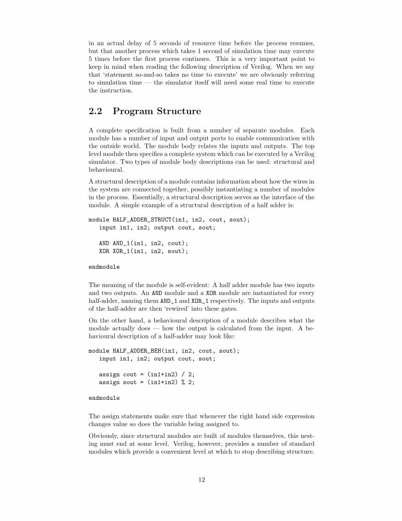
A complete specification is built from a number of separate modules. Eachmodule has a number of input and output ports to enable communication withthe outside world. The module body relates the inputs and outputs. The toplevel module then specifies a complete system which can be executed by a Verilogsimulator. Two types of module body descriptions can be used: structural andbehavioural.
A structural description of a module contains information about how the wires inthe system are connected together, possibly instantiating a number of modulesin the process. Essentially, a structural description serves as the interface of themodule. A simple example of a structural description of a half adder is:
module HALF_ADDER_STRUCT(in1, in2, cout, sout);
input in1, in2; output cout, sout;
AND AND_1(in1, in2, cout);
XOR XOR_1(in1, in2, sout);
endmodule
The meaning of the module is self-evident: A half adder module has two inputsand two outputs. An AND module and a XOR module are instantiated for everyhalf-adder, naming them AND_1 and XOR_1 respectively. The inputs and outputsof the half-adder are then ‘rewired’ into these gates.
On the other hand, a behavioural description of a module describes what themodule actually does — how the output is calculated from the input. A be-havioural description of a half-adder may look like:
module HALF_ADDER_BEH(in1, in2, cout, sout);
input in1, in2; output cout, sout;
assign cout = (in1+in2) / 2;
assign sout = (in1+in2) % 2;
endmodule
The assign statements make sure that whenever the right hand side expressionchanges value so does the variable being assigned to.
Obviously, since structural modules are built of modules themselves, this nest-ing must end at some level. Verilog, however, provides a number of standardmodules which provide a convenient level at which to stop describing structure.
12

The description of these in-built modules is beyond the scope of this chapterand will not be described any further.
It is also interesting to note that in engineering circles, modules are sometimesdescribed in both ways. Both modules are then combined into a single moduletogether with a test module which feeds a variety of inputs to both modules,and compares the outputs. Since behavioural modules are generally easier tounderstand and write than structural ones, this is sometimes considered to bean empirical basis for ‘correctness’.
2.3 Signal Values
Different models allow different values on wires. The semantic model given inthis thesis deals with a simple binary (1 or 0) type. This is extendable to dealwith two extra values z (high impedance) and x (unknown value). Other modelsallow signals of different strengths to deal with ambiguous situations.
Sometimes it is necessary to introduce internal connections to feed the outputof a module into another. Verilog provides two types of signal propagationdevices: wires and registers. Once assigned a value, registers keep that valueuntil another assignment occurs. In this respect, registers are very similar tonormal program variables. Wires, on the other hand, have no storage capacity,and if undriven, revert to value x.
In this chapter we will be discussing only register variables. For a discussion ofwire type variables one can refer to any one of the main references given at thebeginning of the chapter.
2.4 Language Constructs
Behavioural descriptions of modules are built from a number of programmingconstructs some of which are rather similar to ones used in imperative pro-gramming languages. Four different types of behavioural modules are treatedhere:
Continuous assignments: A module may continuously drive a signal on avariable. Such a statement takes the form:
assign v=e
This statement ensures that variable v always has the value of expressione. Whenever the value of a variable in expression e changes, an update tovariable v is immediately sent.
Delayed continuous assignments: Sometimes, it is desirable to wait for theexpression to remain constant for a period of time before the assignmenttakes place. This is given by:
assign v = #n e
If the variables of e change, an assignment is scheduled to take place in n
units time. Furthermore, any assignments scheduled to take place beforethat time are cancelled. Note that if v can be written to by only one suchstatement, the effect is equivalent to making sure that after the variablesin e change, they must remain constant for at least n time units if thevalue of v is to be updated. This type of delay is called inertial delay.
13

One-off modules: It is sometimes desirable to describe the behaviour of amodule using a program. The following module starts executing the pro-gram P as soon as the system is started off. Once P has terminated, themodule no longer affects any wires or registers.
initial P
Looping modules: Similarly, it is sometimes desirable to repeatedly execute aprogram P. In the following module, whenever P terminates, it is restartedagain:
forever P
The different modules are executed in ‘parallel’ during simulation. Hence, wecan construct a collection of modules which outputs a_changed, a variable whichis true if and only if the value of a has just changed:
assign a_prev = #1 a
assign a_changed = a xor a_prev
2.4.1 Programs
The syntax of a valid program is given in table 2.1. As can be seen, a pro-gram is basically a list of semi-colon separated instructions. If the sequenceof instructions lies within a fork . . . join block, the instructions are executedin parallel, otherwise they are executed in sequence, one following the other.These two approaches can be mixed together. Note that if a parallel block isput into sequential composition with another block, as in fork P;Q join; R,R starts only after both P and Q have terminated.
Instruction blocks can be joined together into a single instruction by the use ofbegin and end. This allows, for example, the embedding of sequential programsin parallel blocks as shown in the following program:
fork begin P;Q end; R join
In this case, Q must wait for P to terminate before executing. On the otherhand, R starts at the same time as P.
The instructions we will be expounding can be split into 3 classes: guards,assignments and compound statements.
Guards
Timed guards: #n stops the current process for n simulation time units afterwhich control is given back.
Value sensitive guards: A program can be set to wait until a particular con-dition becomes true. wait e, where e is an expression, does just this.
Edge sensitive guards: The processing of a process thread can also be pauseduntil a particular event happens on one of the variables. There are threemain commands: @posedge v waits for a transition from a value which isnot 1 to 1 on v; @negedge v waits for a falling edge on variable v; and @v
which waits for either event.
Complex guards: A guard can also be set to wait until either of a number ofedge-events happen. @(G1 or G2 or ... Gn), waits until any of @G1 to@Gn is lowered.
14

〈prog〉 ::= 〈instr〉| 〈instr〉 ; 〈prog〉
〈edge〉 ::= 〈var〉| posedge 〈var〉| negedge 〈var〉| 〈edge〉 or 〈edge〉
〈guard〉 ::= # 〈number〉| wait 〈var〉| @ 〈edge〉
〈inst〉 ::= begin 〈prog〉 end| fork 〈prog〉 join| 〈guard〉| 〈var〉 = 〈expr〉| 〈var〉 = 〈guard〉 〈expr〉| 〈guard〉 〈var〉 = 〈expr〉| 〈var〉 <= 〈guard〉 〈expr〉| if (〈expr〉) 〈inst〉| if (〈expr〉) 〈inst〉 else 〈inst〉| while (〈expr〉) 〈inst〉| do (〈expr〉) while 〈inst〉| forever 〈inst〉| fork 〈prog〉 join
Table 2.1: The syntax of a subset of Verilog
15

Assignments
Immediate assignments: Assignments of the form v=e correspond very closelyto the assignment statements normally used in imperative programminglanguages like C and Pascal. The variable v takes the value of expressione without taking any simulation time at all.
Blocking guarded assignments: There are two types of blocking assignmentstatements: g v=e and v=g e, where g is a guard. Their semantics arequite straightforward — g v=e behaves just like g; v=e and v=g e be-haves like v′=e; g; v=v′ (where v′ is a fresh variable, unused anywhereelse).
Non-blocking guarded assignments: The assignment v<=g e acts just likev=g e, but does not block the execution of any code appearing after it.Thus, for any program P, v<=g e; P acts like:
fork v=g e; P join1
Each of these types of assignments can be used to assign a number of variablesin parallel. For example, v1, v2, ...vn = e1, e2, ...en is interpreted asthe assignment which starts by calculating the values of expressions e1 up to en
(using the old values of variables v1 to vn) and then assigning these values tothe variables at one go. Hence, after executing v=0 ; v,w=1,v, v and w havethe values 1 and 0 respectively.
Constructs
Conditional: The conditional statements if (b) P and if (b) P else Q actjust like their counterpart in imperative programming languages like C andPascal. The value of b is evaluated and, if it is evaluated to 1, executionfollows through the first branch, otherwise through the second branch.
Loops: while (b) P corresponds exactly once again to its counterpart in im-perative programming. b is evaluated and, if true, P is executed. At theend of the execution, control is placed once again at the beginning of thewhile loop. When b is evaluated and is found to be 0, the loop terminates.
do P while (b) acts in a similar fashion, but checks the value of theexpression at the end of the executions, rather than at the start.
forever P is used for non-terminating loops, acting just like while (1) P.
There is obviously much more to Verilog than this. However, this probablyconstitutes the main core of ideas behind the whole language. The informalpresentation of the semantics in this section, still leaves a wide range of possiblebehaviours. We will reduce this by giving the simulation cycle semantics ofthe language. This will, essentially, describe how the language is executed ona simulator and will therefore remove most of the issues still unclear up to thispoint.
1Note that this is only meant as an informal description of the semantics. If we were touse this definition, one of the conditions would have to be that P is the rest of the sequen-tial program. Otherwise, we would have situations where (v<=g e; P); Q does not act likev<=g e;(P;Q), which is undesirable, since it would mean that sequential composition is notassociative.
16
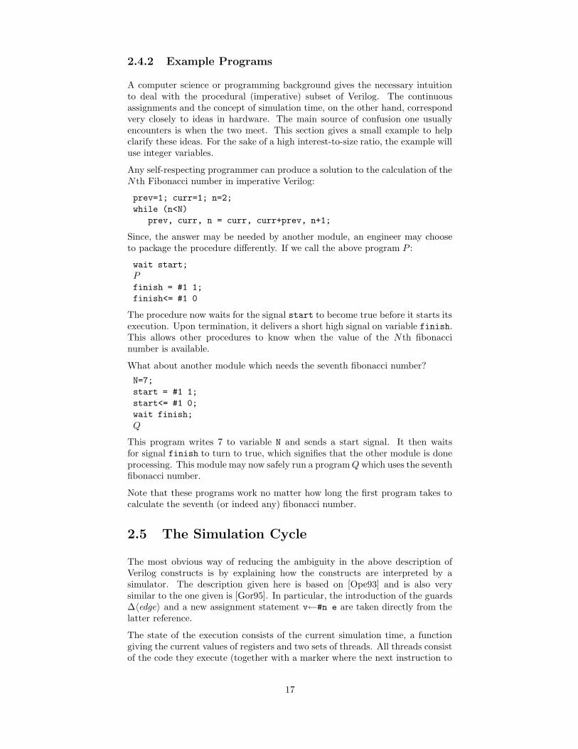
2.4.2 Example Programs
A computer science or programming background gives the necessary intuitionto deal with the procedural (imperative) subset of Verilog. The continuousassignments and the concept of simulation time, on the other hand, correspondvery closely to ideas in hardware. The main source of confusion one usuallyencounters is when the two meet. This section gives a small example to helpclarify these ideas. For the sake of a high interest-to-size ratio, the example willuse integer variables.
Any self-respecting programmer can produce a solution to the calculation of theNth Fibonacci number in imperative Verilog:
prev=1; curr=1; n=2;
while (n<N)
prev, curr, n = curr, curr+prev, n+1;
Since, the answer may be needed by another module, an engineer may chooseto package the procedure differently. If we call the above program P :
wait start;
Pfinish = #1 1;
finish<= #1 0
The procedure now waits for the signal start to become true before it starts itsexecution. Upon termination, it delivers a short high signal on variable finish.This allows other procedures to know when the value of the Nth fibonaccinumber is available.
What about another module which needs the seventh fibonacci number?
N=7;
start = #1 1;
start<= #1 0;
wait finish;
Q
This program writes 7 to variable N and sends a start signal. It then waitsfor signal finish to turn to true, which signifies that the other module is doneprocessing. This module may now safely run a programQ which uses the seventhfibonacci number.
Note that these programs work no matter how long the first program takes tocalculate the seventh (or indeed any) fibonacci number.
2.5 The Simulation Cycle
The most obvious way of reducing the ambiguity in the above description ofVerilog constructs is by explaining how the constructs are interpreted by asimulator. The description given here is based on [Ope93] and is also verysimilar to the one given is [Gor95]. In particular, the introduction of the guards∆〈edge〉 and a new assignment statement v←#n e are taken directly from thelatter reference.
The state of the execution consists of the current simulation time, a functiongiving the current values of registers and two sets of threads. All threads consistof the code they execute (together with a marker where the next instruction to
17

be executed lies), their status and possibly, a pending assignment. The statusof a thread can be one of:
• Enabled
• Delayed until t
• Guarded by g
• Finished
The two sets of threads are called statement threads and update threads.
2.5.1 Initialisation
Initially, the variables are all set to the unknown state x and the simulationtime is reset to 0. Each module is placed in a different statement thread withthe execution point set at the first instruction and with its status enabled.
Simulation Cycle
We start by describing what the execution of a statement in a thread does. Thisobviously depends on the instruction being executed.
Guards: For each type of guard, we specify the actions taking place. We willadd a new type of guard ∆v, where v is an edge. The reason will becomeapparent later.
• #n: The status of the thread is set to: delayed until t, where t is n
more than the current simulation time.
• wait v: If v is true, the thread remains enabled and the executionpoint is advanced. Otherwise, the thread becomes blocked by a guardwhich is lowered when v becomes true.
• ∆e: changes the status to guarded by e, where e is the guard at theexecution point.
• @v, @posedge v, @negedge v and @(g1 or g2 ... or gn): behavejust like the guards ∆v; #0, ∆posedge v; #0, ∆negedge v; #0
and ∆(g1 or g2 ... or gn) ;#0 respectively. The implications ofthis interpretation are discussed in more detail at the end of thissection, once the whole simulation cycle has been described.
Assignments: We consider the different type of assignments separately:
• v=e: e is evaluated and the resulting value is written to variable v.
• g v=e: is treated just like g; v=e.
• v=g e: e is evaluated to α and the thread is set guarded by g. Apending assignment v=α is also added to the thread.
• v<=g e: e is evaluated to α and a new update thread is createdguarded by g and with an assignment statement v=α as its only code.
After this, the execution point of the code is advanced if there are anyfurther instructions. Otherwise, the status of the thread is set to finished.
18

Compound Statements:
• if (b) P: b is evaluated and the execution point is moved to P iftrue, but moved to the end of the whole instruction otherwise.
• if (b) P else Q: b is evaluated and the execution point is advancedinto P or Q accordingly.
• while (b) P: is replaced by if (b) begin P; while (b) P end.
• forever P: is replaced by while (1) P
• fork P join: Creates as many threads as there are statements in P
and sets them all as enabled.
• begin P end: is simply replaced by P.
The complete simulation cycle can now be described:
1. If there are any enabled statement threads, the simulator starts by pickingone. If it has a pending assignment it is executed and the pending assign-ment is removed, otherwise a step is made along the statement code. If achange which has just occurred on a variable lowers other threads’ guards,these threads have their status modified from guarded to enabled, and thesimulator goes back to step 1.
2. If there are any threads delayed to the current simulation time they areenabled and the simulator restarts from step 1.
3. If any update threads are enabled, they are carried out in the order theywere created and the threads are deleted. If the updates have loweredguards on some threads, these have their status reset to enabled. Controlreturns back to step 1.
4. Finally, we need to advance time. The simulator chooses the lowest of thetimes to which statement threads are delayed. The simulation is set tothis time and all threads enabled to start at this time are enabled. Controlis given back to step 1.
Now, the difference between @e and ∆e should be clearer. In (∆e; P), Pbecomes enabled immediately upon receiving the required edge e. On the otherhand, in (@e; P), P is only enabled once the required edge is detected and allother enabled statements in parallel threads are exhausted.
2.5.2 Top-Level Modules
This description of the simulation cycle is limited to programs. How are modulesfirst transformed into programs?
Modules in the form initial P are transformed to P, and modules in the formalways P are transformed to forever P.
Intuitively, one would expect that assign v=e to be equivalent to the modulealways @(v1 or ... or vn) v=e where v1 to vn are the variables used inexpression e. Reading the official documentation carefully, however, shows thatthis is not so. When the assign statement is enabled (by a change on thevariables of e), the assignment is executable immediately. In the other situation,after lowering the guard @(v1 or ... vn), one still has to wait for all other
19

enabled statements to be executed before the assignment can take place. Thus,the continuous assignment is treated in a way analogous to:
always ∆(v1 or ... vn) v=e
This leaves only delayed continuous assignments to be dealt with. The instruc-tion always v=#n e is equivalent to:
always ∆(v1 or ... vn) v← #n e
v←#n e is another type of assignment acting as follows: the current value of eis evaluated (α) and a new statement thread, delayed to n time units more thanthe current simulation time, is created. This new thread has the assignment v=αas its code. Furthermore, all similar statement threads with code v=α and whichare delayed to earlier times are deleted (hence achieving the inertial effect).
2.6 Concluding Comments
We have presented the informal semantics of Verilog in two distinct ways. Inour opinion, neither presentation explains the language in a satisfactory manner.The first presentation lacks enough detail and is far too ambiguous to be usedas a reference for serious work. The second is akin to presenting the semanticsof C by explaining how a C compiler should work. This is far too detailed,and despite the obvious benefits which can be reaped from this knowledge, onecan become a competent C programmer without knowing anything about itscompilation. Having more space in which to expound their ideas, books aboutVerilog usually take an approach similar to our first presentation but give a moredetailed account. They still lack, however, the elegance which can regularly befound in books expounding on ‘cleaner’ languages such as C and Occam. Themain culprits are shared variables and certain subtle issues in the simulationcycle (such as the separate handling of blocking and non-blocking assignments).This indicates that the language may need to be ‘cleaned up’ before its formalsemantics can be specified in a useful manner. This will be discussed in moredetail in chapter 5.
20

Chapter 3
Relational Duration
Calculus
3.1 Introduction
Temporal logics are a special case of modal logic [Gol92], with restrictions placedon the relation which specifies when a state is a successor of another. Theserestrictions produce a family of states whose properties resemble our concept oftime. For example, we would expect transitivity in the order in which eventshappen: if an event A happens before another event B which, in turn, happensbefore C, we expect A to happen before C.
Applications of temporal logics in computer science have been investigated forquite a few years. The applications include hardware description, concurrentprogram behaviour and specification of critically timed systems. The main ad-vantage over just using functions over time to describe these systems is thattemporal logics allow us to abstract over time. We can thus describe systemsusing more general operators which makes specifications shorter, easier to un-derstand and hence possibly easier to prove properties of. They have beenshown to be particularly useful in specifying and proving properties of real-timesystems where delays and reaction times are inherent and cannot be ignored.
The temporal logic used here is the Duration Calculus. It was developed byChaochen Zhou, C.A.R. Hoare and Anders P. Ravn in 1991 [ZHR91]. As withother temporal logics, it is designed to describe systems which are undergo-ing changes over time. The main emphasis is placed on the particular stateholding for a period of time, rather than just for individual moments. Severalapplications of Duration Calculus (henceforth DC) and extensions to the cal-culus have been given in the literature. The interested reader is referred to[Zho93, ZHX95a, ZRH93, ZX95, Ris92, HRS94, HO94, HH94, HO94, MR93] tomention but a few. [HB93] gives a more formal (and typed) description of DCthan the one presented here where the typed specification language Z [Spi92] isused for the description.
3.2 Duration Calculus
3.2.1 The Syntax
We will start by describing briefly the syntax of the DC. The natural and realnumbers are embedded within DC. Then, we have a set of state variables, which
21

〈natural number 〉〈state variables 〉〈state expression〉 ::= 〈state variables 〉
| 〈state expression〉 ∧ 〈state expression〉| 〈state expression〉 ∨ 〈state expression〉| 〈state expression〉 ⇒ 〈state expression〉| 〈state expression〉 ⇔ 〈state expression〉| ¬〈state expression〉
〈duration formula〉 ::=∫〈state expression〉 = 〈natural number〉
| d〈state expression〉e| 〈duration formula〉 ∧ 〈duration formula〉| 〈duration formula〉 ∨ 〈duration formula〉| 〈duration formula〉 ⇒ 〈duration formula〉| 〈duration formula〉 ⇔ 〈duration formula〉| ¬〈duration formula〉| 〈duration formula〉 ; 〈duration formula〉| ∃∃〈state variable〉 · 〈duration formula〉
Table 3.1: Syntax of the Duration Calculus
are used to describe the behaviour of states over time. The constant statevariables 1 and 0 are included.
The state variables may be combined together using operators such as ∧, ∨ and¬ to form state expressions. These state expressions are then used to constructduration formulae which will tell us things about time intervals, rather thantime points (as state variables and state expressions did). Table 3.1 gives thecomplete syntax.
We will call the set of all state variables SV and the set of all duration formulaeDF .
3.2.2 Lifting Predicate Calculus Operators
Before we can start to define the semantics of Duration Calculus, we will recallthe lifting of a boolean operator over a set. This operation will be found usefullater when defining DC.
Since the symbols usually used for boolean operators are now used in DC (seetable 3.1), we face a choice. We can do either of the following:
• overload the symbols eg ∧ is both normal predicate calculus conjunctionand the symbol as used in DC, or
• use alternative symbols for the boolean operators
The latter policy is adopted for the purposes of defining the semantics of DC soas to avoid confusion. The alternative symbols used are: ∼ is not, ∩ is and, ∪is or, → is implies and ↔ is if and only if.
Given any n-ary boolean operator ⊕, from� n to
�, and an arbitrary set S, we
can define the lifting of ⊕ over S, written asS⊕.
22

S⊕ is also an n-ary operator which, however, acts on functions from S to
�, and
returns a function of similar type.
LIFT == S −→ �
S⊕:: LIFTn −→ LIFT
Informally, the functional effect of lifting an operator ⊕ over a set S is to apply⊕ pointwise over functions of type LIFT . In other words, the result of applyingS⊕ to an input (a1, a2, . . . an) is the function which, given s ∈ S acts like applyingeach ai to s and then applying ⊕ to the results.
S⊕ (a1 . . . an)(s)
def= ⊕ (a1(s) . . . an(s))
For example, if we raise the negation operator ∼ over a set � we get an oper-
ator�∼ which given a function from time ( � ) to boolean values (
�), returns its
pointwise negation: for any time t,�∼ P (t) =∼ P (t).
This concept is being defined generally, rather than just applying it wheneverwe need, because we can easily prove that lifting preserves certain propertiesof the original operator such as commutativity, associativity, idempotency, etc.This allows us to assume these properties whenever we lift an operator withouthaving to make sure that they hold each and every time.
3.2.3 The Semantics
Now that the syntax has been stated, we may start to give a semantic meaningto the symbols used. So as to avoid having to declare the type of every variableused, we will use the following convention: n is a number, X and Y are statevariables, P and Q state expressions and D, E and F duration formulae. Givenan interpretation I of the state variables, we can now define the semantics ofDC.
State Variables
State variables are the basic building blocks of duration formulae. State vari-ables describe whether a state holds at individual points in time. We will usethe non-negative real numbers to represent time.
� == � + ∪ {0}Thus, an interpretation of a state variable will be a function from non-negativereal numbers to the boolean values 1 and 0. For any state variable X , itsinterpretation in I, written as I(X), will have the following type:
I(X) :: � −→ {0, 1}The semantics of a state variable under an interpretation I is thus easy to define:
[[X ]]Idef= I(X)
Any interpretation should map the state variables 1 and 0 to the expectedconstant functions:
I(1) = λt : � · 1I(0) = λt : � · 0
23

State Expressions
State expressions have state variables as the basic building blocks. These arethen constructed together using symbols normally used for propositional or pred-icate calculus. We interpret the operators as usually used in propositional cal-culus but lifted over time.
[[X ]]Idef= I(X)
[[P ∧Q]]Idef= [[P ]]I
�∩ [[Q]]I
[[P ∨Q]]Idef= [[P ]]I
�∪ [[Q]]I
[[P ⇒ Q]]Idef= [[P ]]I
�→ [[Q]]I
[[P ⇔ Q]]Idef= [[P ]]I
�↔ [[Q]]I
[[¬P ]]Idef=
�∼ [[P ]]I
where the operators used are the lifting of the normal propositional calculusoperators over time as defined earlier.
Duration Formulae
We now interpret duration formulae as functions from time intervals to booleanvalues. We will thus be introducing our ability to discuss properties over timeintervals rather just than at single points of time. We will only be refering toclosed time intervals usually written in mathematics as [b, e], where both b ande are real numbers. This is formally defined as follows:
[·, ·] :: � × � → � �
[b, e]def= {r : � | b ≤ r ≤ e}
Interval is the set of all such intervals such that b is at most e:
Intervaldef= {[b, e] | b, e ∈ � , b ≤ e}
We can now specify the type of duration formulae interpretation:
[[D]]I :: Interval −→ {0, 1}∫P = n holds if and only if P holds exactly for n units over the given interval.
More formally:
[[∫P = n]]I [b, e]
def=
∫ e
b
[[P ]]Idt = n
dP e is true if the state expression P was true over the whole interval beingconsidered, which must be longer than zero:
[[dP e]]I [b, e] def= (
∫ e
b
[[P ]]Idt = e− b) and (b < e)
24

Now we come to the operators ∧, ∨, ¬, ⇒ and ⇔. Note that these are notthe same operators as defined earlier for state expressions. Their inputs andoutputs are of different types from the previous ones. However, they will bedefined in a very similar way:
[[D ∧ E]]Idef= [[D]]I
Interval∩ [[E]]I
[[D ∨ E]]Idef= [[D]]I
Interval∪ [[E]]I
[[D ⇒ E]]Idef= [[D]]I
Interval→ [[E]]I
[[D ⇔ E]]Idef= [[D]]I
Interval↔ [[E]]I
[[¬D]]Idef=
Interval∼ [[D]]I
These definitions may be given in a style which is simpler to understand bydefining the application of the function pointwise as follows:
[[D ∧ E]]I [b, e]def= [[D]]I [b, e] ∩ [[E]]I [b, e]
We now come to the chop operator ; , sometimes referred to as join or sequentialcomposition. By D ; E we will informally mean that the current interval canbe chopped into two parts (each of which is a closed, continuous interval) suchthat D holds on the first part and E holds on the second. Formally, we write:
[[D ; E]]I [b, e]def= ∃m ∈ [b, e] · [[D]]I [b,m] ∩ [[E]]I [m, e]
Existential Quantification
Standard DC allows only quantification over global variables whereas in IntervalTemporal Logic the quantifier can be used over both global variables and statevariables. We adopt state variable quantification since it will be found usefullater.
Existentially quantifying over a state variable is defined simply as existentiallyquantifying over the function:
[[ ∃∃X ·D]]I is true if there exists an alternative interpretation I ′ such that:
I ′(Y ) = I(Y ) if Y 6= X
and [[D]]I′ = true
3.2.4 Validity
A duration formula is said to be valid with respect to an interpretation I if itholds for any prefix interval of the form [0, n]. This is written as I ` D.
A formula is simply said to be valid if it is valid with respect to any interpretationI. This is written as ` D.
For example, we can prove that for any interpretation, the chop operator isassociative. This may be written as:
` (D ; (E ; F ))⇔ ((D ; E) ; F )
25
3.2.5 Syntactic Sugaring
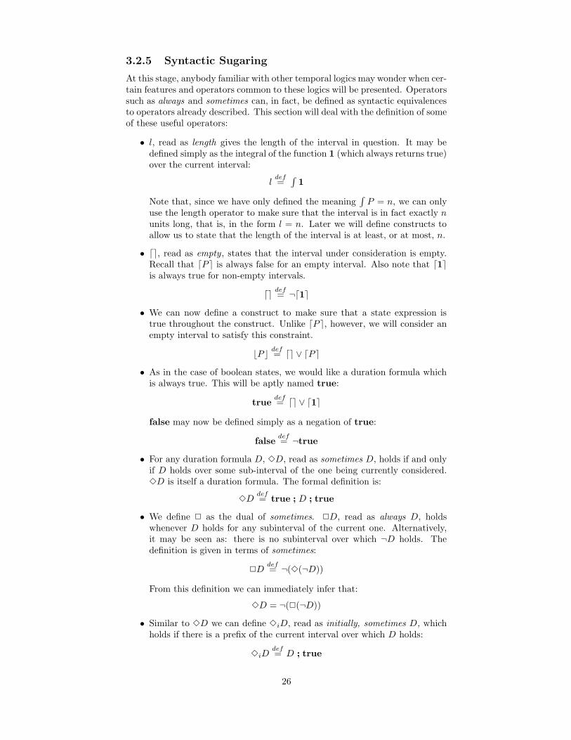
At this stage, anybody familiar with other temporal logics may wonder when cer-tain features and operators common to these logics will be presented. Operatorssuch as always and sometimes can, in fact, be defined as syntactic equivalencesto operators already described. This section will deal with the definition of someof these useful operators:
• l, read as length gives the length of the interval in question. It may bedefined simply as the integral of the function 1 (which always returns true)over the current interval:
ldef=∫
1
Note that, since we have only defined the meaning∫P = n, we can only
use the length operator to make sure that the interval is in fact exactly nunits long, that is, in the form l = n. Later we will define constructs toallow us to state that the length of the interval is at least, or at most, n.
• de, read as empty , states that the interval under consideration is empty.Recall that dP e is always false for an empty interval. Also note that d1eis always true for non-empty intervals.
de def= ¬d1e
• We can now define a construct to make sure that a state expression istrue throughout the construct. Unlike dP e, however, we will consider anempty interval to satisfy this constraint.
bP c def= de ∨ dP e
• As in the case of boolean states, we would like a duration formula whichis always true. This will be aptly named true:
truedef= de ∨ d1e
false may now be defined simply as a negation of true:
falsedef= ¬true
• For any duration formula D, 3D, read as sometimes D, holds if and onlyif D holds over some sub-interval of the one being currently considered.3D is itself a duration formula. The formal definition is:
3Ddef= true ; D ; true
• We define 2 as the dual of sometimes. 2D, read as always D, holdswhenever D holds for any subinterval of the current one. Alternatively,it may be seen as: there is no subinterval over which ¬D holds. Thedefinition is given in terms of sometimes:
2Ddef= ¬(3(¬D))
From this definition we can immediately infer that:
3D = ¬(2(¬D))
• Similar to 3D we can define 3iD, read as initially, sometimes D, whichholds if there is a prefix of the current interval over which D holds:
3iDdef= D ; true
26

• As before, we can define 2iD, read as initially, always D, as follows:
2iDdef= ¬3i¬D
• Recall that we only defined∫P = n as a duration formula. It is usually
the case that we desire to check conditions such as∫P ≤ n or
∫P ≥ n.
These may be defined as:
∫P ≥ n def
=∫P = n ; true
∫P ≤ n def
= ¬(∫P ≥ n) ∨ (
∫P = n)
Note that now the expressions l ≥ n and l ≤ n are duration formulae.
3.3 Least Fixed Point
In expressing certain situations, it may be useful to be able to recursively definetemporal behaviour. In [PR95] P.K. Pandya and Y.S. Ramakrishna introducethe use of the µ notation in the Mean-Value Calculus, a variant of DurationCalculus. This section presents part of this work with respect to the DurationCalculus. The resulting calculus allows for finitely many free variables, andenables us to use finite mutual recursion.
3.3.1 Open Formulae
A duration formula is said to be open if contains a positive number of freevariables. One such formula is l < 5 ∨ (l = 5;X). We will write such formulaeas F (X), where X is the list of free variables in the formulae.
Given an interpretation J of open variables, we can also give the meaning ofopen formulae:
[[X]]JIdef= J (X)
For any other duration formula D, the extended semantics act just as before:
[[D]]JIdef= [[D]]I
3.3.2 Fixed Points
Now consider the recursive equation X = F (X). An interpretation j of variableX is a solution (for a particular I and J ) if:
j = [[F (X)]]J [X←j]I
where J [X ← j] represents the interpretation identical to J except that Xis interpreted as j. The formula given does not necessarily have exactly onesolution. Of these, we will be interested in the least fixed point, which wedenote by µX · F (X).
The concept of least can be expressed informally as ‘the interpretation whichassigns 1 the least possible number of times’. More formally, we say that aninterpretation (of a single variable) i is at least as large as another interpretationj (which we will write as i ≤ j), if any interval for which i returns 1, so does j:
i ≤ j def= i
Interval→ j.
27

3.3.3 Monotonicity
We say that an interpretation J is not larger than J ′, with respect to a variableX if:
• J (Y ) = J ′(Y ) for any Y 6= X , and
• J (X) ≤ J ′(X)
We write this as J ≤X J ′.A formula F is said to be monotonic if:
J ≤X J ′ ⇒ [[F ]]JI ≤ [[F ]]J′
I
3.3.4 Semantics of Recursion
[PR95] goes on to prove a number of useful results. The ones which are ofinterest here are:
• If, in a formula F , X always appears within the scope of an even numberof negations, F is monotonic.
• If F is monotonic in X , then the semantics of µX · F are given by:
Interval∩ {i | [[F ]]J [X←i]I ≤ i}
In other words, it is true for an interval if and only if all interpretationsin V are true over that interval.
• The least fixed point satisfies the following laws:
µX · F (X) = F (µX · F (X))
F (D)⇒ D ` µX · F (X)⇒ D
This construct can, for example, be used to specify a clock signal with period2n in such a way as to expose its iterative nature:
CLOCK1 = (l < n ∧ bCc) ∨ (l = n ∧ dCe);CLOCK0
CLOCK0 = (l < n ∧ b¬Cc) ∨ (l = n ∧ d¬Ce);CLOCK1
These can be combined into:
CLOCK = µX ·
(l < n ∧ bCc)∨ (l = n ∧ dCe); (l < n ∧ b¬Cc)∨ (l = n ∧ dCe); (l = n ∧ d¬Ce);X
28

3.4 Discrete Duration Calculus
In [HO94] Jifeng He and Ernst-Rudiger Olderog reduce the general durationcalculus to a discrete time domain. This serves to simplify the calculus whenevercontinuous time is not required, such as in the description of clocked circuits.The modifications are now described.
The calculus will stand unchanged except for the following assumptions:
1. The state functions may only change values at integer times. In otherwords, any state function has to be constant over open intervals of theform (n, n+ 1) where n is a natural number.
2. Only intervals with integer start and end points are allowed.
3. Because of the previous condition, validity is now reduced to prefix inter-vals of the form [0, n] where n is a natural number.
It will also be useful to introduce a unit interval operator similar to dP e butalso implying that we are considering a unit length interval:
ddP ee def= dP e ∧ l = 1
Since the boolean states are now discrete, rather than continuous, it now makesmore sense to introduce a past, or history operator, which uses past values ofthe state variables or expressions. For a state expression P and natural numbern, n� P , read as P shifted by n, is defined as P but with time shifted n unitsback. Since P is a function defined on the non-negative real numbers, n � Phas to be arbitrarily defined on the first n time units. As a convention, wechoose n � P to be false for this period. Time shift may be formally definedas:
(n� P ) t =
{0 if t < nP (t− n) otherwise
Specifying the clock signal is now possible in a different style, emphasising betterthe alternating value of the clock:
CLOCK = 2(l = 1⇒ ddn� C = ¬Cee)
3.5 Relational Duration Calculus
3.5.1 Introduction
The Problem
As has been shown elsewhere, duration calculus (DC) and other temporal logicsare very useful in describing systems where timing is inherent. When describinga system using DC we can usually take safe estimates about timings. However,certain systems we would like to describe using temporal logics include a non-timed subset which is very difficult to describe using a standard temporal logic.Problems usually arise when we would like to describe strings of consecutivezero time transitions.
When defining the semantics of most hardware description languages in termsof some temporal logic, this is one of the main obstacles which have to be
29

overcome. Most HDLs (such as Verilog HDL and VHDL) have both timed andzero delay transitions (assignments). The non-zero delay transitions are quitereadily described using any temporal logic. However, the zero delay assignmentsprove to be a problem since we expect these zero length transitions to happenconsecutively.
Zero delays are best described as infinitesimal delays. We may thus fit anyfinite number of ‘zero delays’ into any finite interval. Momentary intermediatevalues taken by variables during these infinitesimal transitions are ignored bythe model as a whole, but may still affect other variables.
For example, in the series of assignments: i:=1; j:=i; i:=0, the temporaryvalue 1 of variable i will not be captured by the complete system. Still, itsside-effects should be visible, and we expect j to be set to 1 after the series ofassignments.
The Solution
The approach used here is to define an extension of DC, where these zero timetransitions are treated in a relational way to capture temporary and carried overvalues. Hence the name relational duration calculus.
Despite the problems faced by pure DC, most specifications are only interestedin the stable states of the system. This means that the specification of sucha system can usually be given in pure DC. An implementation may, however,require the use of the relational extension presented here. The embedding of DCwithin our system would thus mean that, in effect, such pure DC specificationscan be directly verified.
The problem of where to introduce this necessary effect now arises. The solutionpresented here introduces a new chop operator. The standard chop operator (;)presented earlier causes problems when dealing with zero delay transitions. Oneexample where the result is not what we expect in this new domain of applicationis:
(de ∧A) ; (de ∧ B) ≡ (de ∧A ∧ B) ≡ (de ∧B) ; (de ∧ A)
The whole idea of sequence is thus lost.
3.5.2 The Syntax and Informal Semantics
Relational duration calculus is built over discrete duration calculus by adding anumber of new operators to handle immediate changes over state variables.
Pre and Post Values of State Variables
We will need a way of examining the value of a state variable just before thecurrent interval begins. This is, in effect, similar to reading an input. ←−v willstand for this value.
Similarly we will need to examine or set values of state variables at the end ofthe current interval. Again, this has a similar connotation to the output of aprocess. −→v is the end value of state variable v.
As a simple example, we may now specify the real meaning of an assignmentv := w as follows: de ∧ −→v =←−w .
30

A New Chop Operator
As already discussed, we will need an alternative chop operator. Given tworelational DC formulae D and E, we can informally describe the meaning ofD followed by E where the post-values of the state variables var in D match
their pre-value in E. This is written as Dvaro
9E and is informally described as
follows:
D E.︷ ︸︸ ︷ . ︷ ︸︸ ︷.↑ ↑ ↑b m e
Dvaro
9E holds over an interval [b, e] if we are able to split the interval into two
parts at a point m such that:
• D holds over [b,m] except for variables overwritten by E at m
• E holds over [m, e] with the inputs being the outputs of D
A more formal definition will be given later.
The Syntax of Relational Duration Calculus
Now that an informal description of the new operators has been given, we maygive a complete description of the relational duration calculus syntax. This isgiven in table 3.2.
We will refer to the set of all duration formulae in the Relational DurationCalculus as RDF .
3.5.3 The Semantics
As the syntax table shows, relational duration calculus has a large subset whichis simply duration calculus. The semantics of that subset are identical to thosegiven for the duration calculus in section 3.2.3 and are not redefined here.
Input and Output Values
The input value of a variable v over an interval [b, e], denoted by ←−v is the valueof v just before time b. If b is zero, it will automatically be false. This may bedefined as:
(←−v = x)[b, e]def=
{false if b = 0
limt→ b− v(t) is equal to x otherwise
−→v is the ‘dual’ of ←−v . It is defined as the right limit of v at the end point of theinterval:
(−→v = x)[b, e]def=
limt→ e+ v(t) is equal to x
We may now define equality between two edge values. If e1 and e2 are edgevalues (that is, of the form ←−v or −→v ):
e1 = e2def= ∃x :
� · (e1 = x ∧ e2 = x)
31

〈boolean〉〈natural number〉〈state variables〉〈state expression〉 ::= 〈state variables 〉
| 〈state expression〉 ∧ 〈state expression〉| 〈state expression〉 ∨ 〈state expression〉| 〈state expression〉 ⇒ 〈state expression〉| 〈state expression〉 ⇔ 〈state expression〉| ¬〈state expression〉
〈edge value〉 ::=←−−−−−−−−−−−〈state variable〉
| −−−−−−−−−−−→〈state variable〉〈duration formula〉 ::= 〈edge value〉 = 〈boolean〉
|∫〈state expression〉 = 〈natural number〉
| d〈state expression〉e| 〈duration formula〉 ∧ 〈duration formula〉| 〈duration formula〉 ∨ 〈duration formula〉| 〈duration formula〉 ⇒ 〈duration formula〉| 〈duration formula〉 ⇔ 〈duration formula〉| ¬〈duration formula〉| 〈duration formula〉
varo
9〈duration formula〉
| 〈duration formula〉 ; 〈duration formula〉| ∃∃〈state variable〉 · 〈duration formula〉
Table 3.2: Syntax of the Relational Duration Calculus
32
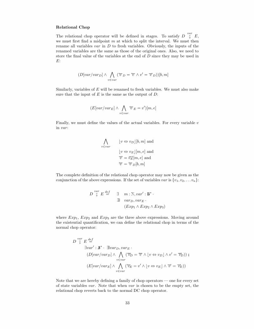
Relational Chop
The relational chop operator will be defined in stages. To satisfy Dvaro
9E,
we must first find a midpoint m at which to split the interval. We must thenrename all variables var in D to fresh variables. Obviously, the inputs of therenamed variables are the same as those of the original ones. Also, we need tostore the final value of the variables at the end of D since they may be used inE:
(D[var/varD ] ∧∧
v∈var
(←−v D =←−v ∧ v′ = −→v D))[b,m]
Similarly, variables of E will be renamed to fresh variables. We must also makesure that the input of E is the same as the output of D:
(E[var/varE ] ∧∧
v∈var
←−v E = v′)[m, e]
Finally, we must define the values of the actual variables. For every variable vin var:
∧
v∈var
bv ⇔ vDc[b,m] and
bv ⇔ vEc[m, e] and−→v = −→vE [m, e] and←−v =←−v D[b,m]
The complete definition of the relational chop operator may now be given as theconjunction of the above expressions. If the set of variables var is {v1, v2, . . . vn}:
Dvaro
9E
def= ∃ m : � , var′ : � ∗ ·
∃∃ varD , varE ·(Exp1 ∧ Exp2 ∧ Exp3)
where Exp1, Exp2 and Exp3 are the three above expressions. Moving aroundthe existential quantification, we can define the relational chop in terms of thenormal chop operator:
Dvaro
9E
def=
∃var′ : � ∗ · ∃∃varD , varE ·(D[var/varD ] ∧
∧
v∈var
(←−vD =←−v ∧ bv ⇔ vDc ∧ v′ = −→vD)) ;
(E[var/varE ] ∧∧
v∈var
(←−vE = v′ ∧ bv ⇔ vEc ∧ −→v = −→vE))
Note that we are hereby defining a family of chop operators — one for every setof state variables var. Note that when var is chosen to be the empty set, therelational chop reverts back to the normal DC chop operator.
33
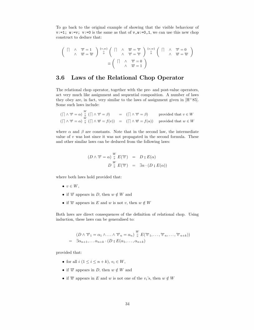
To go back to the original example of showing that the visible behaviour ofv:=1; w:=v; v:=0 is the same as that of v,w:=0,1, we can use this new chopconstruct to deduce that:
(de ∧ −→v = 1∧ −→w =←−w
){v,w}
o
9
(de ∧ −→w =←−v∧ −→v =←−v
){v,w}
o
9
(de ∧ −→v = 0∧ −→w =←−w
)
≡
(de ∧ −→v = 0∧ −→w = 1
)
3.6 Laws of the Relational Chop Operator
The relational chop operator, together with the pre- and post-value operators,act very much like assignment and sequential composition. A number of lawsthey obey are, in fact, very similar to the laws of assignment given in [H+85].Some such laws include:
(de ∧ −→v = α)Wo
9(de ∧ −→v = β) = (de ∧ −→v = β) provided that v ∈W
(de ∧ −→v = α)Wo
9(de ∧ −→w = f(v)) = (de ∧ −→w = f(α)) provided that w ∈W
where α and β are constants. Note that in the second law, the intermediatevalue of v was lost since it was not propagated in the second formula. Theseand other similar laws can be deduced from the following laws:
(D ∧ −→v = α)Wo
9E(←−v ) = D ; E(α)
DWo
9E(←−v ) = ∃α · (D ; E(α))
where both laws hold provided that:
• v ∈W ,
• if −→w appears in D, then w /∈ W and
• if ←−w appears in E and w is not v, then w /∈W
Both laws are direct consequences of the definition of relational chop. Usinginduction, these laws can be generalised to:
(D ∧ −→v 1 = α1 ∧ . . . ∧ −→v n = αn)Wo
9E(←−v 1, . . . ,←−v n, . . . ,←−v n+k))
= ∃αn+1, . . . αn+k · (D ; E(α1, . . . , αn+k)
provided that:
• for all i (1 ≤ i ≤ n+ k), vi ∈ W ,
• if −→w appears in D, then w /∈ W and
• if ←−w appears in E and w is not one of the vi’s, then w /∈ W
34

3.7 Conclusions
Another temporal logic similar to Duration Calculus is Interval Temporal Logic[Mos85]. The main difference between the two is the time domain — DurationCalculus has a dense time domain as opposed to the discrete time domain usedin Interval Temporal Logic. Since asynchronous systems can be expressed morenaturally using a continuous time domain, Duration Calculus (together with itsdiscrete variant) allows immediate comparison of, for instance, the interactionbetween a clocked circuit and a continuous specification of its environment.On the other hand, Interval Temporal Logic allows quantification over statevariables which can be convenient to in temporal abstraction.
Alternative approaches to solve the problem of sequentiality of zero time inter-vals could have been taken. In [ZH96a], Zhou Chaochen and Michael Hansenpropose a similar extension to Duration Calculus to handle immediate assign-ments. The method they use defines the relational chop operator by creatinga small interval between the two over which the two duration formulae can‘communicate’. This extra interval is then abstracted over.
[Qiw96] proposes another similar approach which uses a different interpretationfor state functions. The state functions associate two values for each statevariable at each and every time point which are then used in a very similarfashion to the pre- and post-values described here. The result is used to derivean extension to Hoare logic for reasoning about sequential programs which mayuse DC formulae for time consuming (continuous) sections. The model is notused to handle parallel processes and the elegance of the proofs would probablybe somewhat reduced for such cases.
The main difference between the calculi presented in the above two papers[Qiw96, ZH96a] and Relational DC as presented here is the fact that our chopoperator has a related type. In the other work, the chop operator unifies all thestate variables. In other words, whereas we define a family of chop operators:Wo
9, they have only one chop operator behaving like
varo
9, where var is the set of
all the state variables in the system. This does not reduce expressivity of theother calculi, but it can make certain properties more difficult to state. Forexample, in our case it is quite straightforward to specify a number of durationformulae, each of which controls a number of state variables and which mayinteract (by, for instance, the assignment of a variable to the value of anothervariable controlled by a different formula). These two specifications can usuallyeasily be stated using Relational DC, such that their conjunction correspondsto the behaviour of the composition of the threads obeyed at the same time.
Consider, for example, the statement that w is assigned to 1 after which it isassigned to the value of w ∧ v:
(de ∧ −→w = 1){w}
o
9(de ∧ −→w = (←−w ∧←−v ))
In relational DC this reduces to: −→w =←−v .
However, if we can use only a universal relational chop ({v,w}
o
9in this case), the
above statement changes its meaning to: ∃b :� · −→w = b (which is equivalent to
true).
As already stated, this does not mean that the other calculi are less expressive.There still are ways to state this same property. Obviously, we would rathernot place any constraints on v in this formula (since we might want to give
35

a separate duration formula describing the behaviour of v). So what can bedone if we want to describe multiple variables whose behaviour is defined bydifferent conjuncts? The solution proposed in [ZH96a] uses traces of the sharedvariables. As expected, however, this introduces an extra level of complexity tothe specification, which Relational DC manages without. It is for this reasonthat we believe that for the kind of problems treated in this thesis, RelationalDC is a better candidate than the other similar DC variants.
[BB93] shows how infinitesimal time durations can be included within a tempo-ral process algebra. It would be an interesting project to attempt to integratethe ideas presented in this paper into duration calculus.
Another possible approach investigated elsewhere is the use of timing diagrams[SD97] where the semantics of such an instantaneous change are defined overthe timing diagrams of the function.
One method not explicitly investigated elsewhere is the use of a state baseddiscrete temporal logic where time is simply considered to be another (non-decreasing) variable. One would then define an abstraction over the steps whichdo not increase the value of time to derive a direct relationship between thesequence of states and time steps.
To conclude, the relational duration calculus described in this chapter is onepossible way of defining the semantics of languages which combine both timedand immediate constructs which seems to work reasonably well. The complexityof the definitions may be initially off-putting. However, as in the case of durationcalculus, these definitions should ideally be used to verify a number of algebraiclaws, which can then be used in larger proofs. This way, the ability to simplyspecify certain systems in Relational DC is not spoilt by the complex underlyingsemantics.
36
Chapter 4
Real Time Specifications
This short chapter introduces a number of standard forms for the durationcalculus which can be used to simplify and standardise specifications.
These standard forms help to describe certain commonly encountered real-timeproperties. A number of laws will accompany the standard forms so as toreduce (or altogether remove) the need to revert back to duration calculus toprove results.
These operators were originally introduced in [Rav95, MR93] where the laws westate are also proved.
To illustrate the use of the operators, we will state properties of a simple gas-burner system with three boolean states. Gas will be boolean state true whengas is being released in the system, Flame is true if and only if the gas is ignited,and finally Alarm will represent the state of an alarm, which is to be turned onif too much unburnt gas is released into the system.
4.1 The Real Time Operators
4.1.1 Invariant
A boolean expression is said to be an invariant of the system if it is true at anytime. This will be written as
√P and defined by:
√P
def= bP c
In our example system, one would expect that there is never a flame withoutgas:
√(¬Gas⇒ ¬Flame)
Laws of Invariant
Invariants are monotonic on their only operand:
Law 1: MonotonicIf P ⇒ Q and
√P then
√Q.
Conjunction distributes in and out of invariants:
Law 2: Conjunctive√P ∧√Q =
√(P ∧Q)
37
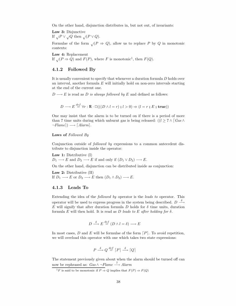
On the other hand, disjunction distributes in, but not out, of invariants:
Law 3: DisjunctiveIf √P ∨√Q then √(P ∨Q).
Formulae of the form√
(P ⇒ Q), allow us to replace P by Q in monotoniccontexts:
Law 4: ReplacementIf√
(P ⇒ Q) and F (P ), where F is monotonic1, then F (Q).
4.1.2 Followed By
It is usually convenient to specify that whenever a duration formulaD holds overan interval, another formula E will initially hold on non-zero intervals startingat the end of the current one.
D −→ E is read as D is always followed by E and defined as follows:
D −→ Edef= ∀r : � ·2(((D ∧ l = r) ; l > 0)⇒ (l = r ; E ; true))
One may insist that the alarm is to be turned on if there is a period of morethan 7 time units during which unburnt gas is being released: ((l ≥ 7 ∧ dGas ∧¬Flamee) −→ dAlarme.
Laws of Followed By
Conjunction outside of followed by expressions to a common antecedent dis-tribute to disjunction inside the operator:
Law 1: Distributive (I)D1 −→ E and D2 −→ E if and only if (D1 ∨D2) −→ E.
On the other hand, disjunction can be distributed inside as conjunction:
Law 2: Distributive (II)If D1 −→ E or D2 −→ E then (D1 ∧D2) −→ E.
4.1.3 Leads To
Extending the idea of the followed by operator is the leads to operator. This
operator will be used to express progress in the system being described. Dδ−→
E will signify that after duration formula D holds for δ time units, durationformula E will then hold. It is read as D leads to E after holding for δ.
Dδ−→ E
def= (D ∧ l = δ) −→ E
In most cases, D and E will be formulae of the form dP e. To avoid repetition,we will overload this operator with one which takes two state expressions:
Pδ−→ Q
def= dP e δ−→ dQe
The statement previously given about when the alarm should be turned off can
now be rephrased as: Gas ∧ ¬Flame7−→ Alarm
1F is said to be monotonic if P ⇒ Q implies that F (P ) ⇒ F (Q)
38
Laws of Leads To
The following laws pertain to the leads to operator with state expressions asoperands.
The leads to operator is monotonic on all three of its operands:
Law 1: Monotonic on delay
If Pδ−→ Q and ∆ ≥ δ then P
∆−→ Q.
Law 2: Monotonic on first operand
If Pδ−→ Q and R⇒ P then R
δ−→ Q.
Law 3: Monotonic on second operand
If Pδ−→ Q and Q⇒ R then P
δ−→ R.
Conjunction distributes in and out of the second state expression:
Law 4: Conjunctive
Pδ−→ Q1 and P
δ−→ Q2 if and only if Pδ−→ (Q1 ∧Q2).
Leads to is transitive:
Law 5: TransitiveIf P
δ1−→ Q and Qδ2−→ R then P
δ1+δ2−→ R.
4.1.4 Unless
Sometimes we want to specify that a state expression, if true, must remain sounless another state expression is true. If P and Q are state expressions, thenthe formula P unless Q is defined by:
P unless Qdef= 2(dP e ; d¬P e ⇒ dP e ; d¬P ∧Qe ; true)
The alarm must not turn off until the gas leak is fixed: Alarm unless ¬(Gas ∧¬Flame).
So as not to have the alarm turning on whenever it feels like it, we can insistthat it remains off until a gas leak occurs: ¬Alarm unless Gas ∧ ¬Flame.
Laws of Unless
The unless operator is monotonic on its second operand:
Law 1: MonotonicIf Q⇒ R and P unless Q then P unless R.
Conjunction distributes into the first operand becoming disjunction:
Law 2: DistributivityIf P1 unless Q and P2 unless Q then (P1 ∨ P2) unless Q.
Conjunction distributes inside the second operand:
Law 3: ConjunctivityIf P unless Q1 and P unless Q2 then P unless (Q1 ∧Q2).
39

4.1.5 Stability
Certain boolean expressions must remain true for a minimum number of timeunits. This stability requirement is written as S(P, δ) and is formally definedas:
S(P, δ)def= 2(d¬P e ; dP e ; d¬P e ⇒ l > δ)
Finally, to ensure that the alarm does not flash on and off we insist that onceit turns on it must remain so for at least 10 time units: S(Alarm, 10).
Laws of Stability
Stability is monotonic:
Law 1: MonotonicIf S(P,∆) and ∆ ≥ δ then S(P, δ).
4.2 Discrete Duration Calculus
Finally, we give a small number of laws which arise from these operators whenwe use discrete duration calculus. These laws were given in [HO94].
Law 1: Discrete leads-toP
δ−→ Q = 2(dd¬Qee ⇒ ∨
0<i≤δddi� ¬P ee)Law 2: Discrete stability (I)S(P, δ) = 2(dd¬P ee ; dP e ; dd¬P ee ⇒ l ≥ δ + 2)
Law 3: Discrete stability (II)If we can find a state expression Q such that 2(
∧
0≤i<nddi � Qee ⇒ dd¬P ee)and 2(
∨
0≤i<n ¬ddi� Qee ⇒ ddP ee) then S(P, n).
4.3 Summary
As already noted elsewhere (for example in [Man81, MP81]) and will be seenlater in this thesis, using a temporal logic to model the semantics of a languageeases the specification and verification of real-time requirements. For this rea-son, a high level real-time specification language is ideal to allow parts of thereasoning to proceed without having to fall back onto reasoning within the tem-poral logic. This chapter describes a number of such operators which will beused later in specifying real-time constraints and properties.
40

Part II
Now that all the necessary tools and notationshave been exposed, we define the formal seman-tics of Verilog and, using these semantics, wepresent a number of algebraic laws which Ver-ilog programs obey.
41

Chapter 5
Formal Semantics of Verilog
5.1 Introduction
5.2 Syntax and Informal Semantics of Verilog
A Verilog specification consists of a number of modules which run in parallel.Each module has an alphabet of local variables which it uses. In additionthere are a number of global variables which act as communication ports ofthe complete system. Recall from chapter 2 that all the variables used will beof register type and, if not assigned a value at the current time, will keep theprevious value.
We will assume that all time delays will be of integer length. If this is notso, we can always multiply all the delays by a constant, so as to satisfy thispre-condition. The original times may later be retrieved by dividing. Note thatthis transformation is possible since we consider only rational constant delaysof which we can only have a finite number.
Each module can either (i) be a continuous assignment (assign), or (ii) executethe module statements endlessly (always s), or (iii) execute the module justonce in the beginning (initial s).
Continuous assignments can be either immediate or delayed. Delayed continuousassignments can be either inertial or transport delayed1.
always and initialmodule instructions are a sequence of statements separatedby the sequential composition operator ;. Each statement can be one of anumber of types:
Skip: Unarguably the simplest instruction. Does nothing and takes no simula-tion time either.
Guards: These delay the execution of the statement sequence for some time.Different guard types are available. The ones we will use are:
• Time delays (#n): This guard blocks the statement sequence for ex-actly n time units.
• Edge sensitive delays (@v, @posedge v, @negedge v): These guardsblock the instruction sequence until an edge of the desired type isseen on variable v. @posedge v waits for a rising edge (v goes from 0
1Strictly speaking Verilog does not support transport delay. This type of delay can, how-ever, be useful and we will see how it can be defined in terms of Verilog instructions later.
42

to 1), @negedge v for a falling edge (v goes from 1 to 0), and @v waitsfor either type. Note that the formal model presented here cannothandle x and z values. Section 5.5.3 discussed this in more detail.
• Value sensitive delay (wait e): wait e blocks execution until ex-pression e becomes true. Note that it does not wait for a rising edge,just for the value, and hence may be enabled immediately.
• Compound guards (g or. . . or h): This guard blocks execution untilat least one of the guards g. . . h is lowered. Note that this is a gener-alisation of Verilog compound guards which may only be of the form@(g1 ... gn).
Assignments: These are the basic building blocks of the language. The lan-guage allows general concurrent assignments. Three types of assignmentsare identified:
• Zero-delay assignments (v=e): The assignment is executed withouttaking any simulation time at all.
• Guarded assignments (v=g e or g v=e): In the case of v=g e, thevalues of the expressions are read, after which a guard block is en-acted and the assignment takes place. When the guard is lowered,the variables are assigned to the values previously read. Once theassignment takes place, the next statement (if any) following the as-signment is enabled. In the case of g v=e, the guard is enacted andthe assignments take place the moment it is lowered.
• Non-blocking assignment(v<=g e): This acts in a similar way asguarded assignments. However, any statements following the assign-ment do not wait for the assignment to terminate to be executed. Inother words, sequential composition following this type of statementis not treated like sequential composition at all, but more like parallelcomposition.
Compound statements: The statements take one or more programs and con-struct more complex programs out of them.
• if b then P else Q: is the same as normal alternation. If b is trueenable P, otherwise enable Q. Upon termination hand control over tothe next statement, if any. The special case with no else clause isalso allowed.
• while b do P: Again, this is the normal iteration construct. If bis currently true execute P, after which return control to the startof the while statement. A similar instruction is the do P while b
construct. In this case, the boolean check is performed at the end ofthe execution of P, not at the beginning. A special case where P isexecuted repeatedly, without checking for any condition, can also beused: forever P.
• A number of instructions can also be executed concurrently usingthe fork ... join construct. Every instruction in P is executedconcurrently, and execution ends once all individual threads end.In Verilog the individual instructions would be separated by semi-colons. To avoid possible confusion, we will allow only binary par-allel composition, written as fork P ‖ Q join, or simply as P ‖ Q.Note that we can still express parallel composition of more than twoprograms: if parallel composition is taken to be right associative,fork P;Q;R join would be written as:
43

fork P ‖ (fork Q ‖ R join) join
• begin P end: This is given just as a means of collecting statementstogether.
Table 5.1 gives a complete overview of the language.
Not all programs generated by this syntax will be acceptable and only the se-mantics of a subset will be formally defined. The restrictions placed on thelanguage correspond to good practice hardware design and simplify the treat-ment of the language considerably.
The restrictions are practically all related to the concept of global and localvariables. We note that a complete system is made up of a number of modulesrunning in parallel. Each of these modules is made up of sequentially composedindividual statements. We will assume that each of these modules has a set oflocal variables (internal wires) which cannot be modified or referred to by anyother module.
There is also a set of global variables (communication registers) from which allmodules may read. These may be considered to be the input and output portsof the modules. The alphabet of a module is defined to be its local variablestogether with the global registers it writes to.
No merge on output wires: It is considered to be good hardware designpractice to avoid joining together the outputs of different components toavoid problems such as short circuits. The alphabets of different moduleshave thus to be pairwise disjoint. Common local variables can be renamedto avoid this, but no more than one process can write to each wire.
In sections 5.4.5 and 5.5.3 we describe how this assumption can be relaxedto enable, for instance, the specification of tri-state devices.
Registers as state holders: Global variables are always to be assigned usinga guarded assignment with a guard which always takes time to be lowered.In other words, zero delayed assignments to output ports are not allowed.This makes sense if we look at each module as a component which musthave an inherent delay and at the global state to be an abstraction of amemory register. Although it limits the language, it is usually consideredgood design practice to build a circuit in this fashion.
Stability of outputs of combinational circuits: When assign statementsare used to express combinational circuits, care must be taken so as notto give rise to any combinational loop by having the output of a combina-tional circuit connected back into itself. Again, this approach is consideredto be good design practice since it avoids problems such as race-conditions.Formalisation of this check is also rather simple to perform (syntactically).
Stability of boolean tests: Blocking guards can only check conditions on en-vironment variables (input ports). Furthermore, variables used in theboolean test of a conditional or a loop must be local (internal) variables.This allows us to look at guards as synchronisation channels between pro-cesses. Since boolean condition checking takes no time at all, the checkmay only be made over local wires.
No interference on shared variables: Global registers may not be read fromand written to simultaneously. This avoids non-determinism and interfer-ence which can appear when we cannot be sure whether a variable valuehas been updated or not at the moment it is read.
44

〈number〉
〈variable〉
〈exp〉
〈bexp〉
〈var-list〉 ::= 〈variable〉| 〈variable〉,〈var-list〉
〈exp-list〉 ::= 〈exp〉| 〈exp〉,〈exp-list〉
〈guard〉 ::= #〈number〉| @〈variable〉| @posedge 〈variable〉| @negedge 〈variable〉| wait 〈variable〉| 〈guard〉 or 〈guard〉
〈statement〉 ::= skip
| 〈var-list〉=〈exp-list〉| 〈var-list〉=〈guard〉 〈exp-list〉| 〈guard〉 〈var-list〉 = 〈exp-list〉| 〈guard〉| 〈variable〉<=〈guard〉 〈exp〉| if 〈bexp〉 then 〈statement〉 else 〈statement〉| if 〈bexp〉 then 〈statement〉| while 〈bexp〉 do 〈statement〉| do 〈statement〉 while 〈bexp〉| forever 〈statement〉| begin 〈stmt-list〉 end| fork 〈statement〉 ‖ 〈statement〉 join
〈stmt-list〉 ::= 〈statement〉| 〈statement〉 ; 〈stmt-list〉
〈module〉 ::= initial 〈stmt-list〉| always 〈stmt-list〉| assign 〈variable〉=〈exp〉| assign 〈variable〉=#〈number〉 〈exp〉| assignT 〈variable〉=#〈number〉 〈exp〉| 〈module〉 ‖ 〈module〉
Table 5.1: The syntax of a subset of Verilog
45

No super-steps: Using loops in a timed language can be rather dangerous.One must always make sure that loops cannot block the advance of timeby providing an infinite number of steps to be executed before time canbe moved forward.
5.3 The Formal Semantics
5.3.1 The Techniques Used
The semantics of Verilog will be described using Relational Duration Calculus.The relational chop operator is crucial in the semantics, since it allows the simpledescription of zero delayed assignments.
As already discussed, a distinction has to be made between local and globalvariables. We will assume that different processes have disjoint local alphabets.The set of global variables is also assumed to be disjoint from the local variables.A simple syntactic check may be done to ascertain these assumptions. If anyname clashes exist, renaming will solve the problem.
Here, we will use the letters u, v, . . . z to stand for the local or global variables,and we will specify whenever a particular variable can be only local or global.U, V will be lists of variables. e, f will be used to represent expressions suchas u OR v, and E,F lists of such expressions. P, Q, R will be used for variablesrepresenting arbitrary chunks of code. b, c will stand for boolean expressions.D and E will stand for arbitrary duration formulas.
We will also use a function start(e), which, given an expression e, will modifyindividual variables v in the expression to ←−v . For example, the expressionstart(u or v) is←−u or ←−v . This function may be easily defined using primitiverecursion on the structure of expressions.
var(e) is defined to be the set of variables used in expression e.
Finally, we note that we will be defining the meaning of primitive instructionsin terms of continuation semantics and a set of variables it can write to. Forstatement P in the language, we will not define its semantics [[P]], but [[P]]W (D)— the semantics of P writing to variables W such that after the termination ofP, the behaviour is described by duration formula D. In other words we willdefine the semantics of P continued by D with the extra information that thevariables in W are written to by P . The type of the semantics is thus:
[[·]] :: Prog → � SV → RDF → RDF
The full semantics of the higher level instructions are then given in terms ofthe continuation semantics of the constituent instructions. Unless otherwisespecified, any relational chop operator appearing in the definition of [[P]]W (D)will have type W . Thus, for simplicity of presentation, o
9will be used to stand
forWo
9.
Note that the set W will be the set of local variables and global registers towhich the current process can write.
This approach to giving the semantics of Verilog specifications is necessary sincethe semantics of certain instructions (such as non-blocking assignments) dependon what happens after the instruction is executed. Thus, in general one cannotsay that [[P ;Q]] = [[P ]]; [[Q]].
46

5.3.2 Syntactic Equivalences
Before we start defining the semantics of Verilog, we will introduce some syn-tactic equivalences for Relational Duration Calculus formulae which will makethe expression of the semantics more compact and hence simpler to follow.
• Sometimes it is necessary to state that two state variables behave similarlyover the current interval:
P ≈ Q def= bP ⇔ Qc ∧ ←−P =
←−Q ∧ −→P =
−→Q
• We will need to be able to rename state variables. D[Q/P ] read as D withP for Q is defined as follows:
D[Q/P ]def= ∃∃P · (D ∧ P ≈ Q)
• It is frequently necessary to state that a state variable has remained con-stant over the current time interval.
Const(P )def= P ≈ 1 ∨ P ≈ 0
It will be convenient to overload this operator to act on sets:
Const(S)def=∧
P∈S Const(P )
• A conditional operator will simplify descriptions of complex systems. Thiswill be written asD/E.F , and readD if E else F . It is defined as follows:
D / E . Fdef= (E ∧D) ∨ (¬E ∧ F )
The algebraic laws usually associated with the similarly defined operatorin programming languages also hold here. Some such laws are:
D / true . E = DD / false . E = E
E /D . E = E idempotencyE /D . (F / D . G) = (E /D . F ) / D . G associativity
5.3.3 The Primitive Instructions
Skip
This is the simplest of instructions to define. skip followed by a durationformula D simply behaves like D.
[[skip]]W (D)def= D
Unguarded Assignments
The informal meaning of v=e is that v takes the value of e. This assignmenttakes no detectable time. Formally, we define the meaning of v=e followed by aduration formula D as follows:
[[v=e]]W (D)def= (−→v = start(e) ∧ Const(W − {v}) ∧ de) o
9D
Extending these semantics for concurrent assignments is rather straightforward.If V = (v1, . . . , vn) is a variable list with corresponding expression list E =(e1, . . . , en), then:
47

[[V=E]]W (D)def= (
n∧
i=1
−→vi = start(ei) ∧ Const(W − V ) ∧ de) o
9D
Guards
Guards block a process from continuing execution until a certain event happens,or a number of time units elapse. We can divide guards into two separategroups: simple and compound. Simple guards are of the form @v, @posedge v,@negedge v, wait v or #n. Compound guards are of the form g1 or . . . or gn
where each gi is a simple guard.
The most straightforward way of defining the semantics of general guards is todivide the definition into two parts: blocked and continued. blocked representsthe possibility of the guard not yet being lowered whereas continued is used todescribe the behaviour of the guard once it is eventually lowered. In both cases,the variables to which the current process can write remain unchanged. Thesemantics of a guard can be described by:
[[g]]W (D)def= (Const(W ) ∧ blocked) ∨
(Const(W ) ∧ continued) o
9D)
The natural relation between blocked and continued can be expressed as: con-tinued holds exactly the first time unit that blocked does not continue to hold,or, more formally:
continued ⇔ ¬ blocked ∧(de ∨ (2i blocked) ; l = 1)
Thus, defining blocked is sufficient. Also, we always expect that if blocked holds,it also holds for any prefix of the current interval:
blocked ⇔ 2i blocked
These properties can be verified for all guards definined in this chapter. Fur-thermore, we can use these properties to prove other laws we would expect tohold for blocked and continued. For example, we would expect that if a guardis blocked, it has not yet continued (and vice-versa): blocked ⇔ ¬3i continued.This can be proved on the basis of the above two properties.
For every simple guard g we will give the expressions for blocked and continued.The next section will then extend this idea for compound guards.
• [[#n]]W (D)
This is the simplest guard. It is not lowered until n time units have elapsed.It allows the process to continue after precisely n time units elapse.
blockeddef= l < n
continueddef= l = n
• [[@v]]W (D)
This guard is lowered once a rising or falling edge is detected on variablev.
48

blockeddef= (bvc ∧ −→v = true)
∨ (b¬vc ∧ −→v = false)
continueddef= (dve ∧ −→v = false)
∨ (d¬ve ∧ −→v = true)
• [[@posedge v]]W (D)
This is similar to the previous guard but sensitive only to rising edges.
blockeddef= bvc ∨ (bvc ; b¬vc ∧ −→v = false)
continueddef= bvc ; d¬ve ∧ −→v = true
• [[@negedge v]]W (D)
This is identical to posedge v but sensitive to falling rather than risingedges.
blockeddef= b¬vc ∨ (b¬vc ; bvc ∧ −→v = true)
continueddef= b¬vc ; dve ∧ −→v = false
• [[wait v]]W (D)
wait v waits until v becomes true. The only difference between this andposedge v is that this does not wait for a rising edge, and may thus beactivated immediately.
blockeddef= b¬vc ∧ −→v = false
continueddef= b¬vc ∧ −→v = true
Compound Guards
Having defined the semantics for simple guards, we can now easily extend theidea for a complex guard of the form:
(g1 or . . .or gn)
From the previous section, we know blockedi and continuedi for each guard gi.These will now be used to work out blocked and continued for the complexguard. Rather than define the semantics of a general guard with n componentguards, only the special case with two component guards is considered.
A double guard (g1 or g2) is blocked whenever both the constituent guards areblocked. It continues once either of the guards is lowered. We must make surethat the combined guard is lowered once the first of the individual guards islowered. In other words, up to one time unit ago, both guards must still havebeen blocked. Formally, this translates to:
49

blockeddef= blocked1 ∧ blocked2
continueddef= (de ∨ (blocked1 ∧ blocked2) ; l = 1) ∧
(continued1 ∨ continued2)
When manipulating the expressions it is clear that this operation is commu-tative, associative and idempotent. The associativity justifies the lack of useof brackets in complex guards (without specifying whether it is left or rightassociative). Furthermore, the semantics of a general complex guard can besimplified to:
blockeddef=
n∧
i=1
blockedi
continueddef= (de ∨ (
n∧
i=1
blockedi ; l = 1)) ∧
n∨
i=1
continuedi
Guarded Assignments
Given an assignment of the form V=g E, where g is a guard, we can now easilydefine its semantics in terms of the semantics of the guard itself. By ‘remember-ing’ the value of E at the beginning, we can define the semantics of the guardedassignment statement simply as the sequential composition of the guard followedby a zero-delay assignment of the variable to the remembered value of E:
[[V=g E]]W (D)def= ∃∃α · [[α=E ; g ; V=α]]W (D)
The semantics of sequential composition will be given later.
For a guarded assignment of the form g V=E, the semantics are even simpler:
[[g V=E]]W (D)def= [[g ; V=E]]W (D)
5.3.4 Constructive Operators
Conditional
The semantics of if-then-else statements follow in a rather natural fashion.If the boolean guard is true at the start of the time interval the statementbehaves just like the then branch of instruction, otherwise it behaves like theelse branch.
[[if b then P else Q]]W (D)def= [[P]]W (D) / start(b) . [[Q]]W (D)
Conditionals with no else clause can also be defined:
if b then P ≡ if b then P else skip
Note that sometimes, we will also use the shorthand notation P / b . Q for theVerilog program if (b) then P else Q.
50
Iteration
The while statement is defined using recursion.
[[while b do P]]W (D)def= µX · [[P]]W (X) / start(b) . D
Sometimes, we will use b*P as shorthand for while (b) P.
The do P while b construct is very similar and can be viewed as a special caseof the while b do P statement:
do P while b ≡ P; while b do P
This will sometimes be abbreviated to P*b.
Verilog also provides another loop statement: forever P. As expected, P isrepeatedly executed forever. Its semantics may thus be defined by replacingall forever statements with while statements and using the semantics alreadydefined.
forever P ≡ while (true) do P
Sequential Composition
Thanks to the continuation semantics used, sequential composition is trivial todefine. The semantics of P;Q followed by D can be defined as the semantics ofP followed by the semantics of Q followed by D.
[[P;Q]]W (D)def= [[P]]W ([[Q]]W (D))
An immediate conclusion we can draw from this definition is the associativityof sequential composition in Verilog.
Internal Parallel Composition
We will use the term internal parallel composition to refer to the fork . . . join
operator as opposed to the external parallel composition between modules.
Composing two programs in parallel will act just like running both at the sametime with the execution of the continuation resuming as soon as both programsterminate. Note that the output variables W of the process will be dividedbetween the two processes such that P controls WP and Q controls WQ. Thevariable sets must partition W ie W = WP ∪WQ and WP ∩WQ = ∅.
[[fork P ‖ Q join]]W (D)def=
([[P]]WP
(Const(WP ) o
9D) ∧ [[Q]]WQ
(D))∨ [[Q]]WQ
(Const(WQ) o
9D) ∧ [[P]]WP
(D))
)
An immediate corollary of this definition is that internal parallel composition iscommutative and associative.
51

5.3.5 Top-Level Instructions
At the top-level, we can now specify the complete semantics of a module withoutneeding to take into consideration what happens afterwards. These instructionsmay thus be interpreted as closure operators — producing a closed system froman open one.
Initial Statements
Informally initial P specifies that P will be executed once at the beginning.
[[initial P]]def= [[P]]αP(Const(αP))
The alphabet of P, αP, is the set of the local variables used in the process P andalso all the global variables assigned to by this process. These variables may beobtained using a syntactic pass over P. It must be made sure that the alphabetsof different processes are pairwise disjoint.
Infinite Loops
always P specifies that P will be repeatedly executed forever. This is equivalentto repeating P indefinitely at the beginning:
always P ≡ initial (forever P)
Continuous Assignments
Another type of module is the assign module, which performs a continuousassignment. In this section, only the semantics of immediate assign modulesare considered. The case with a delay between the input and output is discussedin a later section.
The module assign v=e makes sure that whenever expression e changes value,v immediately gets the new value. This behaviour is practically identical tothat of a combinational circuit, where there is practically no delay between theinput and output of the component. The semantics of such a statement arestraightforward to define:
[[assign v=e]]def=√
(v = e)
One must make sure that no combinational circuits arise from such statementssince such situations may lead to infinite changes in zero time. Two examplesshowing this type of infinite behaviour are:
assign v = ¬vassign v = ¬w ‖ assign w = ¬v
A simple syntactic check suffices to ensure that no such behaviour can arise. Itis discussed in detail in section 5.5.1.
52

Parallel Components
Given two top-level instructions in parallel, we will simply define their combinedsemantics as:
[[P ‖ Q]] def= [[P]] ∧ [[Q]]
Note that the following law justifies the use of internal parallel composition todescribe the fork ...join construct:
(initial P
‖ initial Q
)
≡ initial fork P ‖ Q join
This also justifies the use of P ‖ Q as shorthand for fork P ‖ Q join.
5.4 Other Extensions to the Language
5.4.1 Local Variables
It is sometimes desirable to declare local variables to make code more readable.The semantics of such a construct can be formalised as follows:
[[var v; P; end v;]]W (D)def= ∃∃v · [[P]]W∪{v}(D)
For simplicity we assume that v is not in W . To relax this restriction, we wouldfirst rename the variable to a fresh instance and then use the semantics givenabove.
5.4.2 Variable Initialisation
It is usually very useful to initialise global registers to particular values. Thisis not possible because of the restriction that all assignments to such registersmust be time guarded. However this restriction may be slightly weakened byintroducing a new instruction:
〈initialisation〉 ::= init 〈var-list〉 = 〈bool-list〉〈module〉 ::= initial 〈initialisation〉; 〈statement〉
| forever 〈initialisation〉; 〈statement〉...
As expected, the variables in the initialisation list must be output variables ofthe current module.
The semantics extend naturally for this new construct:
[[initial init V=E; P]]def= [[initial V=E;P]]
[[always init V=E;P]]def= [[initial V=E; forever P]]
In most cases, the init keyword will be left out since its presence can be deducedimmediately.
53

5.4.3 Delayed Continuous Assignments
Delayed continuous assignments behave like inertial delays between the inputand the output: whenever a change in the input wires is noticed, an assignmentof the input expression to the output is set to be executed after the delay. Anyother assignment to the same variable due to execute before the new assignmentis removed. In other words, the output changes value once the inputs have allremained constant for the specified delay.
[[assign v = #n e]]def=
(l < n ∧ b¬vc)
∨ (l = n ∧ d¬ve); true
)
∧
(∃b · dvar(e) = be) n−→ dv = n� ee ∧¬ (∃b · dvar(e) = be) n−→ dv = 1� ve
where b is a sequence of boolean values of the same length as the sequence ofvariables var(e). Thus, if the variables in expression e remain unchanged for n
time units, v takes that value, while if any of the variables have changed value,v keeps its old value.
Notice that this behaviour does not fully encompass the behaviour of the assignstatement in Verilog. Whenever the variables in the expression remain constantfor exactly n time units, the simulator semantics allows one of two sequences ofexecution:
1. The change on one of the variables of e takes place before the assignmentof v and thus pre-empts the upcoming assignment.
2. The assignment to v takes place before the change of value of the variablein expression e.
This situation thus leads to a non-deterministic choice, with the behaviour de-pending on how the simulator is implemented. This situation is undesirablesince the result does not fully describe the (intuitive) corresponding hardware.More complex examples may exhibit even more unexpected behaviour. Ourview is that a more hardware related approach is to take the behaviour as al-ready described. The simpler, more direct semantics are easier to handle andto prove results in.
Hence, to make sure that these formal semantics correspond directly to thesemantics of actual Verilog, one would have to make sure that changes to thevariables in expression e would never occur exactly n time units apart. If onthe other hand one is viewing these semantics from a hardware point of view,where the delayed continuous assignment corresponds to a high capacitancedelay, these semantics should be adequate.
Note that assign v=#n e guarantees that v does not change more often thanevery n time units: S(v, n) and S(¬v, n).
5.4.4 Transport Delay
Another type of delayed assignment is transport delayed assignment. As op-posed to inertial delay, an event on the variables on the right hand side ofthe assignment take place no matter whether any other change occurs before
54

the actual assignment takes place. Later, it will be shown how transport de-lay can be implemented as several inertial delays in sequence. Also, since wewould like our approach to be extendible and applicable to other hardwaredescription languages, we will also be using transport delay in the coming chap-ters. For this reason, we introduce a continuous transport delay assignment:assignT v=#n e.
[[assignT v=#n e]]def=
√(v = n� e)
5.4.5 Non-Blocking Assignments
Non-blocking assignments behave just like blocking assignments except thatthe next statement in the module executes immediately without waiting forthe assignment to terminate. Note that this may introduce concurrent threadscontrolling the same variables and thus the parallel composition operator alreadydefined fails to correctly describe the semantics. The solution we opt for isbased on the concept of parallel by merge as described and expounded upon in[HJ98]. The basic underlying idea is that each process controls a copy of theshared variables, which are then merged into the actual variable when parallelcomposition is performed. [HJ98] use this basic idea to generalise differentforms of parallel composition ranging from shared clock parallel programs toconcurrent logic programs. This approach is mentioned again in section 5.5.3,where resolution functions are discussed.
The semantics of non-blocking assignment are defined by:
[[v<=c e]]W (D)def= [[v=c e]]{v}(Const(v)) ‖
{v}D
Since both processes running in parallel can control the variable v, they arecomposed together using a merging parallel composition operator. This operatorallows for common variables to be changed by more than one process. Whenevera variable is assigned to by both processes it non-deterministically takes one ofthe values it is assigned to. It should now be clear that it is necessary to maintainan extra boolean state for every Verilog variable v: assignv, which holds in thosetime slots when variable v has just been assigned a value.
The semantics of the merging parallel composition is given by renaming thecommon variable and then merging the two together:
[[P ‖{v}
Q]]W (D)def= ∃∃vP , vQ, assignvP
, assignvQ·
P [vP , assignvP/v, assignv] ∧
Q[vQ, assignvQ/v, assignv] ∧
Merge(vP , vQ, v)
Merge(v1, v2, v) manages variable v as a merging of the two variables v1 and v2.Obviously, assignv is true exactly when either of assignv1
and assignv2is true.
Furthermore, for any time unit, the value of v is:
• the same as v1 whenever v1 has just been assigned a value, but not v2,
• the same as v2 whenever v2 has just been assigned a value, but not v1,
• the same as the previous value of v whenever neither v1 nor v2 have justbeen assigned,
55

• a non-deterministic choice between v1 and v2 when both have just beenassigned a value.
Formally, this can be written as:
Merge(v1, v2, v)def= bassignv = assignv1
∨ assignv2c ∧
2(ddassignv1∧ ¬assignv2
ee ⇒ ddv = v1ee) ∧2(ddassignv2
∧ ¬assignv1ee ⇒ ddv = v2ee) ∧
2(ddassignv1∧ assignv2
ee ⇒ ddv = v1 ∨ v = v2ee) ∧2(dd¬assignv1
∧ ¬assignv2ee ⇒ ddv = 1� vee)
Obviously, the state variables assignv need to be maintained by the model. Thisis done by adding the information that assignv is true immediately after anassignment:
[[v=e]]W (D)def= (de ∧ −−−−→assignv = true ∧ −→v = start(e) ∧ Const(W − {v})) o
9D
Also, whenever a variable is kept constant with Const(v) we make sure thatassignv does not become true:
Const’(v)def= Const(v) ∧ (de ∨ (l = 1 ∧ Const(assignv)) o
9(b¬assignvc ∧ −−−−→assignv = false)
In other words, assignv keeps the value it has just been assigned prior to thecurrent interval but then reverts to zero after one time unit.
Since a shared variable is not considered local, any input from a shared variablev is changed to read from vin. At the topmost level, it would then be necessaryto add the invariant:
√vin = v.
Finally note that the relational chop type is no longer the same as the alphabetof the process (W ) but:
W ∪ {assignv | v ∈ W}As can be seen from the above discussion, using non-blocking assignments canconsiderably complicate the model. However, the extra information does notinvalidate proofs about sub-systems which do not use non-blocking assignments.In fact, it is possible to split the semantics of a process into the conjunction oftwo separate parts: one controlling the variable values and the other recordingwhether the variables have been assigned to. If the program has no non-blockingassignments, the first conjunct will be identical to the semantics of the programas given in a previous section. In brief, proofs on programs not using non-blocking assignments can be done using the previous, simpler model. The extrainformation about assignv would only be necessary in modules which use suchassignments.
A difference from standard Verilog is that, in our case, blocking and non-blockingassignments have the same priority. In the case of standard Verilog, this isnot true, and changes to variable values induced by non-blocking assignmentsare executed only when no other changes are possible. The model presentedhere may be extended to deal with priority (possibly by introducing multi-levelsignal strengths) but we choose to stay at a weaker, less deterministic level. Forexample consider the program v<=#1 1; v=#1 0. In Verilog, v would alwaysend up with value 1, since the normal (blocking) assignment v=#1 0 would beexecuted before the non-blocking assignment of v to 1. The semantics presented
56
here would not guarantee this, and it would be possible to show only that after1 time unit v has value 1 or 0.
A more hardware oriented view is not to allow multiple drivers to assign a valueto the common output at the same time. This may effectively lead to a shortcircuit, thus making the resultant circuit dangerous and its behaviour chaotic.The semantics of parallel merging would look like:
[[P ‖{v}
Q]]W (D)def= ∃∃vP , vQ, assignvP
, assignvQ·
2(b¬assignvP∨ ¬assignvQ
c)⇒ . . .
Whenever a multiple assignment takes place, the result would thus be chaos(true) which implements only the trivial specification.
5.5 Discussion
5.5.1 Avoiding Combinational Loops
To avoid the possibility of combinational loops, it is sufficient to perform asyntactic check. This check can be formalised by defining a dependency relationcon(P), where, if (v,w) is in the relation, then v is connected to w.
con(assign v=e)def= {(v,w) | w is a variable in e}
con(initial P)def= ∅
con(always P)def= ∅
con(P‖Q) def= (con(P) ∪ con(Q))+
where R+ is the transitive closure of relation R.
To check that a program P has no combinational feedback, it is enough to makesure that no wire is related to itself, or formally, that:
con(P) ∩ Id = ∅where Id is the identity relation over the set of wires.
5.5.2 Time Consuming Programs
From the restrictions placed on Verilog, it is clear that we would like to assesswhether an instruction always take time to execute or not. To do this we willdefine dur(P), meaning that P must always take time to execute, as follows:
dur(wait v)def= false
dur(@v)def= true
dur(@posedge v)def= true
dur(@negedge v)def= true
dur(#n)def= true iff n > 0
57

dur(g1 or g2)def= dur(g1) ∧ dur(g2)
dur(v = e)def= false
dur(v = g e)def= dur(g)
dur(g v = e)def= dur(g)
dur(skip)def= false
dur(if b then P else Q)def= dur(P ) ∧ dur(Q)
dur(while b do P)def= false
dur(P ; Q)def= dur(P ) ∨ dur(Q)
dur(fork P ‖ Q join)def= dur(P ) ∨ dur(Q)
For any sequential program P, we can now show whether dur(P) is true or not.Note that it is possible to show that if dur(P) is true, the execution of P takestime to terminate:
([[t=0;P;t=1]]W (Const(W )) ∧ −→t = 1) ⇒ l > 0
It is now possible to formalise some of the restrictions:
• Body of loops must take time: To use while b do P, dur(P) must be true.
• Guarded assignments to global registers: If v is a global register, andthe current process can write to it, then v=g e and g v=e are acceptableprovided that dur(g) is true.
The second restriction can be relaxed by making sure that any two assignmentsto a global variable are separated by a program of non-zero duration.
5.5.3 Extending Boolean Types
Verilog users may prefer to use the four valued logic with {x, 0, 1, z} rather thanthe two valued one that is presented here. Such a system can be implemented byhaving two boolean states describing the value of the variables. For a variable w,w.m will be true if w has a meaningful value (0 or 1) and w.v will specify whetherthe value is high or low (the value is either 1 or z if w.v is true). This extendedmodel is more complex and in many cases using 1 and 0 values is sufficient. Itis for these reasons that the semantic values were limited to the two booleanones.
An important use of the z and x values is when designing tri-state devices[Pal96, SSMT93]. Obviously, in this case, simply adding the extra values willnot suffice since, in general, one would desire to have multiple drivers on thesame variables and possibly also use resolution functions to arbitrate resultantvalues. Parallel merging is, once again, the way one could model such a situation.As before, each process writes to a local variable, where all these local values arethen cascaded together using the merge operator. For example, in the case of abidirectional bus where one device may want to send a high impedance value z
to allow the other device to write a value, the part of the merge operator whichmanages this situation would look like the following:
58

√(v1 = z⇒ v = v2)
Once again notice the extra information which needs to be carried around tohandle this kind of situation. Also, due to the nature of the parallel merge oper-ator, which acts as a closure operator, our model loses some of its compositionalaspects.
5.5.4 Concurrent Read and Write
The major constraint on the language is the fact that we do not allow con-current read and write between processes. This constraint can be removed bymaking the reading of non-local variables in assignment statements take eitherthe previous or next value non-deterministically. This should guarantee soundsemantics even if we allow processes to read and write concurrently. However,the semantics will still not be complete since, for example, we would still not beable to prove that at the end of @posedge v; w=v the variable w has value 1.
5.6 Related Work
The main aim of [Goo93b] was to analyse how structure and behaviour interactin HDL specifications. However, it is one of the best overviews of the differentapproaches taken to formalise HDL behaviour as of 1993. Unfortunately, it ex-clusively discusses continuous assignment style specifications with no imperativeprogramming features.
Since then considerable work which formalises HDLs has appeared. However, aswe note in the introduction, not much work has been done on Verilog itself. Anotable exception is the VFE (Verilog Formal Equivalence) project [GG95] setup by the M.J.C. Gordon and D.J. Greaves. [Gor95] set the scene for researchbeing done by the VFE project and also served as direct inspiration for thiswork. [Gor98] shows how programs written in a subset of Verilog can be trans-lated into Mealy machines hence enabling formal analysis of these programs.In [GG98] the interpretation is done down to a RTL (Register Transfer Level)specification language which is given a mathematical semantics. Two levels ofsemantics are discussed: simulation (or event) semantics discuss the behaviourat the simulation cycle level while trace semantics abstract over unstable andintermediate states. Two other semantic levels are identified but not yet anal-ysed.
Most of the work done on industry standard HDLs, however, tends to deal withVHDL. Anthologies of formal semantics for VHDL have appeared in [KB95] and[Bor95].
A popular approach is to give an operational semantics to emulate the HDLsimulation cycle. [Goo95] gives an operational semantics to VHDL, while [Tas90,TH91, Tas92] use HOL to formally specify the behaviour of the simulation cycle.The popularity of this sort of semantics for HDLs is natural, since most of theintricate behaviour is closely related to the way the languages are simulated. Inour case, we prefer to restrict the language to give a more elegant and abstractsemantics.
Other approaches have also been reported in the literature. Of particular in-terest is [WMS91] which proposes a semantics of VHDL based on an intervaltemporal logic. The authors formalise a relatively large subset of VHDL butleaving out delta delays. To deal with the relational-temporal nature of the
59

language they use an interesting mechanism, whereby the behaviour is firstspecified in terms of steps in resource (as opposed to simulation) time, eachof which corresponds to a simulator instruction execution. This is then ab-stracted away by introducing a global clock (counting simulation time) whichsynchronises the different behaviour traces. The resultant semantics convey theexpected behaviour, but time related specifications in the resultant model lackhigh level abstraction.
Other denotational approaches have appeared in [BS95, BFK95, Dav93]. Inparticular, [BFK95] gives an elegant semantics using the idea of a world-lineand current time point to describe the state. This semantics is then used todefine an equivalent axiomatic semantics for VHDL. Various other approacheshave been tried, most of which are far too detached from our presentation tomerit discussion in detail. [KB95] is a good starting point for such research.
5.7 Conclusions
The semantics of the basic language are quite easy to handle. As we includeother features, the semantics grow more and more complicated. This indicatesthe need for algebraic laws to reason about the language in a more abstract fash-ion. These laws will be given in chapter 6. An attractive part of the languagesemantics design is its modularity. One can reason about a program whichuses only blocking assignments using the simple semantics. If a non-blockingassignment is to be added to the program, the behaviour of the extra booleanstates can be derived separately. Also, provided that there is no interferencebetween the non-blocking assignment and the already existent program, all pre-vious results shown are still valid. This compositional approach to languagesemantics promotes and gives the opportunity to follow good and sound designmethodologies.
60

Chapter 6
Algebraic Laws
6.1 Introduction
Having defined the semantics of the language in question, one can prove proper-ties about programs. However, proving properties in terms of relational durationcalculus can, at times, be very tedious. Sometimes we would simply like to trans-form a given implementation into an equivalent one, or refine a program into amore efficient version. Following the approach as used in [H+85, RH86, HMC96]we give a number of algebraic equalities (and inequalities) which are satisfiedby any Verilog program. These laws can be verified with respect to the seman-tics given in the previous chapter, thus allowing us to prove results using theselaws rather than having to fall back onto the underlying semantics. The lawsare given in terms of variables which can be replaced by any arbitrary program(unless there is a side condition which permits its use only on programs whichrespect certain properties).
6.2 Notation
Most of these laws give an equality between two programs. Since we are givinga continuation semantics of the language, it is important to explain what wemean when we say that P = Q. The first condition is that the alphabet of P isthe same as that of Q. The other condition is that for any possible continuation,the two programs behave identically. Formally, this may be written as:
P = Qdef= [[P ]]V (D) = [[Q]]V (D)
where D can range over all valid relational duration formulae with V being thealphabet of both P and Q.
However, in certain cases, full blown equality is far too strong a condition tosatisfy. In such cases, we consider refinements: we say that a programQ refines aprogram P (written as P v Q) if, under all possible continuations, the behaviourof Q implies that of P .
P v Q def= [[Q]]V (D)⇒ [[P ]]V (D)
Again, the implication must be satisfied for any relational duration formula Dwith V being the alphabet of P and Q.
61

Note that equality can be rephrased in terms of refinement as follows:
P = Q ≡ P v Q ∧ Q v P
Note that the left hand side and right hand side of the equalities and inequalitiesmust have the same output alphabet.
6.3 Monotonicity
The first class of laws we will be giving state that the programming constructsin Verilog are monotonic. In other words, if we selectively refine portions of theprogram, we are guaranteed a refinement of the whole program. The proofs ofthese laws are given fully due to their importance. For the rest of the chapterwe will only state the nature of the proof.
The following lemma will be needed to prove some laws in this chapter.
Lemma: For any program P with alphabet W , [[P ]]W is a monotonic function:
D ⇒ E ` [[P ]]W (D)⇒ [[P ]]W (E)
Proof: The proof proceeds by structural induction on the program.
Base cases:
Skip:
[[skip]]W (D)= { by definition of semantics }
D⇒ { by premise }
E= { by definition of semantics }
[[skip]]W (E)
Assignment:
[[v = e]]W (D)= { by definition of semantics }
(−→v = start(e) ∧ Const(W − {v}) ∧ de) o
9D
⇒ { by monotonicity of relational chop and premise }(−→v = start(e) ∧ Const(W − {v}) ∧ de) o
9E
= { by definition of semantics }[[v = e]]W (E)
Guards:
[[g]]W (D)= { by definition of semantics }
(gnt ∧ Const(W )) ∨ ((gter ∧ Const(W )) o
9D)
⇒ { by monotonicity of relational chop and disjunction and premise }(gnt ∧ Const(W )) ∨ ((gter ∧ Const(W )) o
9E)
= { by definition of semantics }[[g]]W (E)
62
Inductive cases:
Sequential composition:
[[Q;R]]W (D)= { by definition of semantics }
[[Q]]W ([[R]]W (D))⇒ { inductive hypothesis on [[Q]]W and [[R]]W }
[[Q]]W ([[R]]W (E))= { by definition of semantics }
[[Q;R]]W (D)
Conditionals:[[if b then P else Q]]W (D)
= { by definition of conditional }[[P ]]W (D) /
←−b . [[Q]]W (D)
⇒ { monotonicity of DC conditional, inductive hypothesis and premise }[[P ]]W (E) /
←−b . [[Q]]W (E)
= { by definition of conditional }[[if b then P else Q]]W (E)
Loops:
[[while b do P ]]W (D)= { by definition of semantics }
µX · [[P ]]W (X) /←−b . D
⇒ { monotonicity, inductive hypothesis and premise}µX · [[P ]]W (X) /
←−b . E
= { by definition of semantics }[[while b do P ]]W (E)
Internal parallel composition:
[[fork P; Q join]]W (D)= { by definition of semantics }
([[P ]]WP(Const(WP ) o
9D) ∧ [[Q]]WQ
(D))∨ ([[P ]]WP
(D) ∧ [[Q]]WQ(Const(WP ) o
9D))
⇒ { monotonicity and inductive hypothesis }([[P ]]WP
(Const(WP ) o
9E) ∧ [[Q]]WQ
(E))∨ ([[P ]]WP
(E) ∧ [[Q]]WQ(Const(WP ) o
9E))
= { by definition of semantics }[[fork P; Q join]]W (E)
Note that the lemma automatically holds for commands defined in terms ofthese instructions and constructs (such as g v=e which is defined as g; v=e).
2
Law: Sequential composition is monotonic:
If P v Q then X ;P v X ;Q and P ;X v Q;X
Note that this law holds only for programs not using non-blocking assignments.
Proof: The lemma is needed to prove monotonicity on the first operand:[[X ;P ]]W (D)
= { definition of semantics }[[X ]]W ([[P ]]W (D))
⇐ { by lemma and premise }[[X ]]W ([[Q]]W (D))
= { definition of semantics }[[X ;Q]]W (D)
63

Monotonicicity on the second operand is easy to establish:[[P ;X]]W (D)
= { definition of semantics }[[P ]]W ([[X ]]W (D))
⇐ { premise }[[Q]]W ([[X ]]W (D))
= { definition of semantics }[[Q;X]]W (D)
2
Law: Parallel composition is monotonic:
If P v Q then X‖P v X‖Q and P‖X v Q‖XProof: Monotonicity on the left operand:
[[P ‖ X]]W (D)= { definition of semantics }
([[P ]]WP(D) ∧ [[X]]WX
(Const(WX) o
9D))
∨ ([[P ]]WP(Const(WP ) o
9D) ∧ [[X ]]WX
(D))⇐ { premise and monotonicity }
([[Q]]WQ(D) ∧ [[X ]]WX
(Const(WX) o
9D))
∨ ([[Q]]WQ(Const(WQ) o
9D) ∧ [[X]]WX
(D))= { definition of semantics }
[[Q ‖ X]]W (D)
The proof for the second branch follows identically.2
Law: Conditionals are monotonic:
If P v Q then X / b . P v X / b . Q and P / b . X v Q / b . X
Proof: Monotonicity of the left branch program:[[P / b . X]]W (D)
= { definition of semantics }[[P ]]W (D) /
←−b . [[X]]W (D)
⇐ { premise and monotonicity }[[Q]]W (D) /
←−b . [[X ]]W (D)
= { definition of semantics }[[Q / b . X ]]W (D)
The proof for the second branch follows identically.2
Law: Loops are monotonic:
If P v Q then b ∗ P v b ∗Q and P ∗ b v Q ∗ bProof: Monotonicity of while loops on their only operand:
[[b ∗ P ]]W (D)= { definition of semantics }
µX · [[P ]]W (X) /←−b . D
⇐ { premise and monotonicity }µX · [[Q]]W (X) /
←−b . D
= { definition of semantics }[[b ∗Q]]W (D)
64

Monotonicity of repeat loops then follows immediately:P ∗ b
= { by definition }P ; b ∗ P
v { by monotonicity of while loops and sequential composition }Q; b ∗Q
= { by definition }Q ∗ b
2
As with monotonicity of sequential composition, this law holds only in the se-mantics of the language without non-blocking assignments.
These laws justify the use of algebraic representation. In other words, if we havea program context C(P ), then we can guarantee that
1. if P v Q then C(P ) v C(Q). This follows directly from the laws justgiven and structural induction on the context C.
2. if P = Q then C(P ) = C(Q). This follows from the equivalence betweenequality and refinement in both directions and point 1.
6.4 Assignment
Normally, in Verilog, immediate assignments do not follow the normal lawsof assignment statements, as for instance used in [H+85]. For example, theprogram v=~v; v=~v is not equivalent to v=v, since a parallel thread may chooseto read the input at that very moment. Another possibility is that the spikewill trigger an edge guard.
In our case, the semantics we give to Verilog are for a specific subset of Verilogprograms for which this equality holds. The problem has been bypassed bynot allowing programs to read and write simultaneously. Also, spikes are notpossible since assignments to global variables cannot be instantaneous.
The laws in this section follow immediately from the semantics of assignmentand the definition of relational chop. In fact, as already mentioned in chapter3, relational chop and pre- and post-values act almost like assignment, providedthat unchanged variables are explicitly stated to be so. The following laws arevery similar (and in some cases identical) to those in [H+85].
Law: Composition of immediate assignments:
v=e;w=f = v,w=e,f[e/v]
v=e;v=f = v=f[e/v]
These rules for combining single assignments can be generalised to parallel as-signments:
Law: Parallel assignments can be commuted:
V=E = πV=π(F)
where π is a permutation.
This commutativity property is used to simplify the presentation of the parallelassignment composition law:
65

Law: Composition of parallel immediate assignments:
U,V=E,F;U,W=G,H = U,V,W=G[E,F/U,V],F,H[E,F/U,V]
where variable sequences V and W have no elements in common.
Since concurrent read and write is not allowed, we have the following law:
Law: Assignments distribute in and out of parallel composition:
(V=E; P) ‖ Q = V=E; (P ‖ Q)To prove this law it is sufficient to note that the behaviour of Q is not affectedby an initial change in the value of variable list V which can be proved bystructural induction on the program.
If we are using the semantic model which does not allow for non-blocking as-signments, an assignment of a variable to itself has no noticeable effect:
Law: Skip and self-assignment (using the semantics which do not allow fornon-blocking assignments):
v=v = skip
The law follows immediately from the fact that (de ∧ Const(W )) acts like the
left one ofWo
9. Note that if non-blocking assignments are used, the behaviour of
the assignment can cause a situation where multiple values are assigned to thesame variable at the same time.
Law: Programs and assignment — provided that P does not assign to v or freevariables in e, all variables in e are in the output alphabet of P and v is notfree in e:
v=e; P = v=e; P; v=e
Again, this law holds provided that there are no non-blocking assignments to v.The proof follows by structural induction on P to show that the post-value ofv remains constant, as does that of e. The proof fails if we take the semanticswhich handle non-blocking assignment since the right hand side program guar-antees that the post-value of assignv is true whereas the left hand side programdoes not.
6.5 Parallel and Sequential Composition
Sequential composition is associative with skip as its left and right unit:
P ; (Q;R) = (P ;Q);R
P ; skip = P
skip;P = P
These laws follow immediately from the definition of skip and associativity offunctional composition.
The following laws about parallel composition hold for internal parallel compo-sition (using the fork ...join construct). The following law, however, allowsmost of these laws to be applied equally well to top-level parallel composition:
66

initial P ‖ initial Q = initial fork P ‖ Q join
This law follows from the fact that Const(W )Wo
9Const(W ) = Const(W ).
Parallel composition is commutative and associative with skip as its unit:
P ‖ Q = Q ‖ PP ‖ (Q ‖ R) = (P ‖ Q) ‖ RP ‖ skip = P
The laws follow from associativity and commutativity of conjunction.
For programs which take time to execute (dur(P ) holds), #1 is also a unit of thecomposition. This can be proved by structural induction on programs satisfyingdur(P ).
Provided that dur(P ):
P ‖ #1 = P
In fact #1 distributes in and out of parallel composition:
#1;P ‖ #1;Q = #1; (P ‖ Q)
Law: If P and Q have different output alphabets, we can show that composingP with Q refines P :
P v (P ‖ Q)1
The main application of this law, is when we choose to refine individual parallelthreads independently. Thus, for example, if we prove that Pi v P ′i (i rangingfrom 1 to n), we can use induction on n and this law to deduce that:
P1 ‖ . . . ‖ Pn v P ′1 | . . . ‖ Pn
1Note that this law cannot be applied if Q has a non-empty output alphabet (since the leftand right hand side would have different output alphabets). To solve this problem, we canintroduce a new program chaosV which allows the variables V to change non-deterministically.
[[chaosV ]]V (D) = true
Clearly, any program outputting to V is a refinement of this program:chaosV v P
This allows us to deduce the intended meaning of the parallel composition law, since P v P ,the above law and monotonicity of parallel composition enable us to deduce:
(P ‖ chaosV ) v (P ‖ Q)
where V is the output alphabet of Q.
67

6.6 Non-determinism and Assumptions
Restricting ourselves to the Verilog constructs can be problematic when provingcertain properties. Sometimes it is useful to introduce certain new constructswhich may feature in the middle part of the proof but would eventually beremoved to reduce the program back to a Verilog program. This approach isused extensively in the correctness proofs of the hardware compiler in chapter10.
One useful construct is non-deterministic composition. Informally, the non-deterministic composition of two programs can behave as either of the two.More formally, we define the semantics of non-determinism (u) as:
[[P uQ]]W (D)def= [[P ]]W (D) ∨ [[Q]]W (D)
From this definition it immediately follows that non-determinism is commuta-tive, associative, idempotent and monotonic:
P uQ = Q u PP u (Q u R) = (P uQ) u R
P u P = P
If P v Q then P uR v Q u Rand R u P v R uQ
Non-determinism also distributes over sequential composition since disjunctiondistributes over relational chop:
P ; (Q u R) = (P ;Q) u (P ;R)
(P uQ);R = (P ;R) u (Q;R)
Another useful class of statements we will use are assumptions. The statementassume b, expressed as b>, claims that expression b has to be true at that pointin the program:
[[b>]]W (D)def= (de ∨ dbe; true) ∧D
false> and true> are, respectively, the left zero and one of sequential compo-sition:
false>;P = false>
true>;P = P
Conjunction of two conditions results in sequential composition of the condi-tions:
(b ∧ c)> = b>; c>
68

This law follows immediately from simple Duration Calculus reasoning. Twocorollaries of this law are the commutativity and idempotency of assumptionswith respect to sequential composition:
b> = b>; b>
b>; c> = c>; b>
Disjunction of two conditions acts like non-determinism:
(b ∨ c)>;P = (b>;P ) u (c>;P )
Assumptions simply make a program more deterministic:
P v b>;P
This holds since prepending an assumption to a program P simply adds anotherconjunct to the semantics of P .
6.7 Conditional
The conditional statement is idempotent and associative:
P / b . P = P
P / b . (Q / b . R) = (P / b . Q) / b . R
These properties follow immediately from the definition of the semantics of con-ditional and idempotency and associativity of Duration Calculus conditionals.
Sequential, parallel and non-deterministic composition distributes out of condi-tionals:
(P / b . Q);R = (P ;R) / b . (Q;R)
P u (Q / b . R) = (P uQ) / b . (P u R)
P ‖ (Q / b . R) = (P ‖ Q) / b . (P ‖ R)
Finally, a number of laws can be given which convey better the meaning of theconditional statement:
P / true . Q = P
P / b . Q = Q / ¬b . PP / b . (Q / b . R) = P / b . R
(P / b . Q) / b . R = P / b . R
Again, these laws follow from the definition of the semantics and the laws ofconditional in Duration Calculus.
69

Provided that the values of the variables in expression b are not changed im-mediately by programs P and Q, a conditional can be expressed in terms ofnon-determinism and assumptions:
P / b . Q = (b>;P ) u (¬b>;Q)
In the language considered for hardware compilation (see chapter 10), the pre-condition is always satisfied. In the general language, one would have to checkthat P (Q) has a prefix P1 (Q1) such that dur(P1) (dur(Q1)) and the variablesof b are not assigned in P1 (Q1).
6.8 Loops
The recursive nature of loops can be expressed quite succinctly in terms ofalgebraic laws:
Law: Unique least fixed point: Q = (P ;Q) / b . skip if and only if Q = b ∗ P .
As immediate corollaries of this law, we can show that:
(b ∗ P ) / b . skip = b ∗ PQ = P ;Q if and only if Q = forever P
Q = P ; (Q / b . skip) if and only if Q = P ∗ b
Law: The first law can be strengthened to: Q = (P ;Q) / b . R if and only ifQ = (b ∗ P );R.
The following law allows us to move part of a loop body outside:
Law: If Q;P ;Q = Q;Q then (P ;Q) ∗ b = P ; (Q ∗ b).The unique fixed point law is one of the more interesting laws presented in thischapter, and we will thus give a complete proof of the result.
Lemma 1: If dur(P ) holds, then there exist relational duration formulae D1
and D2 such that, for any relational duration formula D:
[[P ]]W (D) = D1 ∨ (D2 ∧ l ≥ 1)Wo
9D
where D1 and D2 are independent of D.
Proof: The proof proceeds by induction on the structure P with the followinginductive hypothesis:
[[P ]]W (D) = D1 ∨ (D2 ∧ l ≥ 1)Wo
9D if dur(P )
[[P ]]W (D) = D1 ∨D2
Wo
9D
The proof follows in a routine manner and is thus left out.2
Lemma 2: If dur(P ) holds and l ≤ n⇒ Q = R, then:
l ≤ n+ 1⇒ P ;Q = P ;R
70

Proof:[[P ;Q]]W (D)
= { by definition of semantics }[[P ]]W ([[Q]]W (D))
= { by lemma 1 }D1 ∨ (D2 ∧ l ≥ 1) o
9([[Q]]W (D))
= { l ≤ n+ 1 and chop definition }D1 ∨ (D2 ∧ l ≥ 1) o
9(l ≤ n ∧ [[Q]]W (D))
= { premise }D1 ∨ (D2 ∧ l ≥ 1) o
9(l ≤ n ∧ [[R]]W (D))
= { l ≤ n+ 1, chop definition and monotonicity of DC operators }D1 ∨ (D2 ∧ l ≥ 1) o
9([[R]]W (D))
= { by lemma 1 }[[P ]]W ([[R]]W (D))
= { by definition of semantics }[[P ;R]]W (D)
2
Lemma 3: ∀n : � · (l ≤ n⇒ D = E) if and only if D = E.
Proof: Follows immediately from the underlying axiom ∃n : � · l = n.2
To avoid long mathematical expressions, we will now define:
F (α)def= if b then (P ;α) else skip
We will also be referring to multiple applications of F to an arbitrary programα:
F 1(α)def= F (α)
Fn+1(α)def= F (Fn(α))
Lemma 4: If α is a solution of the equation X = F (X), then α is also asolution to X = F n(X), for any positive integer n.
Proof: The proof follows immediately from the definition of F i(X):
Base case: X = F (X) = F 1(X).
Inductive case:X
= { premise }F (X)
= { monotonicity of F and inductive hypothesis }F (Fn(X))
= { by definition of F n+1 }Fn+1(X)
2
Theorem: If α and β are solutions of the equation X = F (X) and dur(P ),then α = β.
Proof: By lemma 3, it is sufficient to prove that:
∀n : � · l ≤ n⇒ α = β
71

We will now show by induction on n, that this is true for any value of n.
Base case: n = 0
We start by proving the following equality:l ≤ 0 ∧[[P ;α]]W (D)
= { by definition of semantics }l ≤ 0 ∧[[P ]]W ([[α]]W (D))
= { by lemma 1 }l ≤ 0 ∧(D1 ∨ (D2 ∧ l ≥ 1) o
9([[α]]W (D)))
= { DC reasoning about interval length }l ≤ 0 ∧D1
= { DC reasoning about interval length }l ≤ 0 ∧(D1 ∨ (D2 ∧ l ≥ 1) o
9([[β]]W (D)))
= { by lemma 1 }l ≤ 0 ∧[[P ]]W ([[β]]W (D))
= { by definition of semantics }l ≤ 0 ∧[[P ;β]]W (D)
We will now use this equality to prove the base case of the induction:[[α]]W (D)
= { by lemma 4 }[[F (α)]]W (D)
= { by definition of F }[[if b then (P ;α) else skip]]W (D)
= { by definition of semantics }[[P ;α]]W (D) /
←−b . D
= { monotonicity of conditional, l ≤ 0 and previous result }[[P ;β]]W (D) /
←−b . D
= { by definition of semantics }[[if b then (P ;β) else skip]]W (D)
= { by definition of F }[[F (β)]]W (D)
= { by lemma 4 }[[β]]W (D)
This concludes the base case of the theorem.
72

Inductive case: n = k + 1[[α]]W (D)
= { by lemma 4 }[[F k+1(α)]]W (D)
= { by definition of F k+1 }[[F (F k(α))]]W (D)
= { by definition of F }[[if b then (P ;F k(α)) else skip]]W (D)
= { by inductive hypothesis, lemma 2 and monotonicity of conditional }[[if b then (P ;F k(β)) else skip]]W (D)
= { by definition of F }[[F (F k(β))]]W (D)
= { by definition of F k+1 }[[F k+1(β)]]W (D)
= { by lemma 4 }[[β]]W (D)
2
From this theorem we can conclude that:
Corollary: Q = (P ;Q) / b . skip if and only if Q = b ∗ P .
Proof: (⇒) By definition, b ∗ P satisfies the equation X = F (X). By the firstequation, so does Q. Hence, by the theorem Q = b ∗ P .
(⇐) We simply unravel the loop once.2
6.9 Continuous Assignments
Continuous assignments with no delay can be applied syntactically. This is adirect consequence of Duration Calculus invariants’ laws:
(assign v=e(x)
‖ assign x=f
)
=
(assign v=e(f)
‖ assign x=f
)
If variable w is stable for at least 2 time units, we can transform a transportdelay into a number of unit inertial delays. Provided that S(w, 2) and S(¬w, 2):
assignT v=#n w = var v0, . . .vn
assign v1=w
‖ni=2 assign vi=#1 vi−1
‖ assign v=vn
end v0, . . .vn
Note that this law cannot be used if w is not a single variable (since inertialdelay is triggered not when the value of the whole expression changes but whenthe value of any of the variables in the expression changes).
For convenient presentation of certain properties, we will also allow programsof the form P; assign v=e. This will act like:
[[P ]]W ([[assign v=e]] ∧ Const(W − {v}))Similarly, P; (assign v=e ‖ Q) acts like:
[[P ]]W ([[assign v=e ‖ initial Q]])
73

6.10 Communication
The use of synchronisation signals can greatly increase the readability of code.This type of communication can be handled using the subset of Verilog we areusing.
These ‘channels’ can be implemented as global variables which have a normalvalue of zero, but go briefly up to one when a signal is sent over them. ‘Waitfor signal’, s?, is thus easily implemented by:
s?def= wait s
The method used in the Fibonacci number calculator in section 2.4.2 to senda signal on s was by using the following code portion: s=#1 1;s<=#1 0. Notethat this program blocks the execution of future events along this thread by onetime unit, which we would rather avoid.
To send a signal, without blocking the rest of the program for any measurablesimulation time but leaving the signal on for a non-zero time measure, the non-blocking assignment statement can be quite handy:
s!def= s = 1 ; s <= #δ 0
So what value of δ is to be used? Obviously, δ has to be larger than zero.However, taking a value of 1 or larger leads to a conflict in the program:
s! ; #δ ; s!
The solution is to use a value of 0.5 for δ. This may seem to invalidate allthe previous reasoning based on discrete time. However, this is not the case.Effectively, what we have done is to reduce the size of the smallest time step to alevel which normal Verilog programs will not have direct access to. Alternatively,one could have used a value of one for δ and multiplied all delays in the programby a factor of two (effectively allowing Verilog programs to use only even sizeddelays).
If non-blocking assignments are only used for signals, and signals are accessedonly using s! and f(s)?, we can guarantee the monotonicity of sequential com-position and loops despite the presence of non-blocking assignments.
6.11 Algebraic Laws for Communication
6.11.1 Signal Output
Processes which write to a signal s are assumed to do so only using the commands! (except for initialisation). We will use s! ∈ P as shorthand for the (syntactic)check whether the command s! occurs anywhere in program P . Similarly, s! /∈ Prefers to the converse. In both cases, it is assumed that s is in the outputalphabet of P .
Signals start off as false, provided that they are not initially written to:
initial P ;Q = initial ¬s>;P ;Q
provided that dur(P ) and s! /∈ P . The law can be proved by structural inductionon program P .
74

s! sets signal s to true:
s! = s!; s>
Between two programs which do not signal on s, both of which take time toexecute, s is false:
P ;Q = P ;¬s>;Q
provided that s! /∈ P ;Q and dur(P ) and dur(Q). Again, structural induction onP and Q is used to prove this property.
Output on a signal can be moved out of parallel composition:
(s!;P ) ‖ Q = s!; (P ‖ Q)
The proof is almost identical to the similar law which moves assignments out ofparallel composition.
Signalling and assumptions commute:
s!; b> = b>; s!
6.11.2 Wait on Signal
Waiting stops once the condition is satisfied:
(s>;P ) ‖ (s?;Q) = (s>;P ) ‖ Q
Follows immediately from the definition of the semantics of s?.
Execution continues in parallel components until the condition is satisfied:
(¬s>;P ;Q) ‖ (s?;R) = ¬s>;P ; (Q ‖ s?;R)
provided that s! /∈ P . As before, follows from the semantics of s?.
If we also add the constraint that dur(P ), we can even afford an extra time unit:
(¬s>;P ;Q) ‖ (#1; s?;R) = ¬s>;P ; (Q ‖ s?;R)
75

6.11.3 Continuous Assignment Signals
Sometimes, it may be necessary to have signals written to by continuous as-signments. The laws given to handle signal reading and writing no longer applydirectly to these signals and hence need modification.
The following laws thus allow algebraic reasoning about a signal s written to bya continuous assignment of the form:
assign s = f(s1, . . . , sn)
where all variables s1 to sn are signals. For s to behave like a normal signal(normally zero except for half unit long phases with value one), f(0, 0, . . .0) hasto take value 0.
If b⇒ f(s) then:
assign s = f(s) ‖ b>;P = b>; s!; (assign s = f(s) ‖ P )
If b⇒ ¬f(s) and si /∈ P then:
assign s = f(s) ‖ b>;P ;Q = b>;P ; (assign s = f(s) ‖ Q)
To sequentialise outputs on signals si:
assign s = f(s) ‖ si!;P = si!; (assign s = f(s) ‖ s>i ;P )
The above laws are consequences of the following law:
assign s = f(s) ‖ P (s?) = assign s = f(s) ‖ P (f(s)?)
This law is a consequence of Duration Calculus invariants’ laws and the seman-tics of s? and s!.
Furthermore, if P is the process controlling a signal s, and s starts off with avalue 0, the value of f(s) will remain that of f(0) until P takes over.
(s = 0)>; f(s)?;P = (s = 0)>; f(0)?;P
(the underlying assumption is that s is a signal and in the output alphabet ofP ).
6.12 Signals and Merge
Signals now allow us to transform a process to use a different set of variables.The trick used is to define a merging process which merges the assignments ona variable to another.
76

The first thing to do is to make sure that we know whenever a variable has beenassigned to. The technique we use is simply to send a signal on assignv to makeit known that v has just been assigned a value. Note that we will only allowthis procedure to be used on global variables, which guarantees that no morethan one assignment on a particular variable can take place at the same time.
We thus replace all assignments: v=g e by v=g e; assignv! and similarly g v=e
by g v=e; assignv!
The program Merge will collapse the variables v1 and v2 into a single variablev, provided that they are never assigned to at the same time:
Mergedef= var v1, v2, assignv1
, assignv2
assign assignv = assignv1∨ assignv2
‖ assign v = (v1 / assignv1. v2) / assignv . v
−
‖ assign v− = #0.5 v
end v1, v2, assignv1, assignv2
This merge program can be used, for instance to allow parallel programs effec-tively to use the same variables. It also obeys a number of laws which relateMerge to parallel composition and conditional:
(P [v1/v];Q[v2/v]) ‖ Merge = P ;Q
(P [v1/v] / b . Q[v2/v]) ‖ Merge = P / b . Q
Note that for the first law to hold, both sides of the equality must be validprograms.
The laws given in this section follow by structural induction on the programand the laws of invariants (which appear in Merge).
6.13 Conclusions
The aim of this chapter was to identify a number of algebraic laws which Verilogprograms obey. As discussed in [H+85], the formal semantics allow us to lookat programs as mathematical expressions. In mathematics, algebraic laws allowthe manipulation and simplification of programs with relative ease, withouthaving to refer back to the more complex underlying axioms. This is the mainmotivation behind the work presented in this chapter.
77
Part III
This part explores the use of the formal seman-tics. Chapter 7 presents the transformation ofof a real-time specification into a Verilog imple-mentation, while chapter 8 shows how a simplespecification language for simple hardware com-ponents can be defined. A set of laws which de-compose and eventually implement componentsin Verilog by following a simple decision proce-dure are also given and are used in a number ofsimple examples in chapter 9. Other examplesof the use of these semantics for verification canalso be found in [PH98].
78

Chapter 7
A Real Time Example
7.1 Introduction
One of the advantages of Verilog over most software languages is the controlover the passage of time. This makes it possible to implement time sensitivespecifications realistically. This chapter considers a standard real-time spec-ification, and analyses its implementation in Verilog. The implementation isconstructed, rather than divined, thus reducing the number of proofs necessary.This example should also indicate how general principles can be defined to beused to convert standard sections of a specification into correct code.
The example considered is that of a railway level crossing, using the real-timespecification language based on duration calculus presented in chapter 4. Thespecification is a combination of evolution and stability constraints. These en-sure that the system evolves and changes when required, but will not do sounnecessarily.
The contribution of this chapter is to show how one can derive a (correct)Verilog implementation of an abstract specification. The specification is takenfrom [HO94] where a clocked circuit implementation is also proved correct. Theimplementations strategies differ considerably, since we have more abstract con-structs at our disposal. The approach used in this chapter is much more con-structive than that used in [HO94]. The resulting implementations are quitedifferent although they have a similar flavour, which may indicate that thespecification language is already rather low level.
7.2 System Specification
7.2.1 The Boolean States Describing the System
We consider a railway crossing with a gate, traffic lights and railtrack.
1. The environment will provide information as to whether the gate is openor closed. The boolean states to represent these conditions are:
• O for open
• C for closed
2. The environment will also provide information whether the track is emptyor occupied by an approaching train:
79

• E for empty
• A for approaching
3. The implementation must provide the environment with a signal to startopening or closing the gate:
• Oing for opening
• Cing for closing
4. The implementation will also be responsible for setting the traffic lightsred, yellow and green:
• R for red
• Y for yellow
• G for green
Note that we still have no restrictions implying that only one of the states can betrue at any one time. Up to this point all boolean states are independent of oneanother. Thus, for instance, E and A can still both be satisfied simultaneously— the track being empty and occupied at the same time!
7.2.2 System Requirements
We will now list the requirements of the railway crossing. The requirements willbe stated in terms of a specification constant ε. By designing an implementationin terms of ε, we will effectively have designed a family of implementations, fora family of specifications.
• Closing Gate
Once a train starts approaching, the gate must start closing within 15+ εtime units:
Req1def= A
15+ε−→ Cing
Within ε time units, the light must not be green, but yellow or red:
Req2def= A
ε−→ (Y ∨R)
If 3 + ε time units elapse with the gate closing but it has not yet closed,the light must be red:
Req3def= (Cing ∧ ¬C)
3+ε−→ R
• Opening Gate
After just ε time units with the track empty, the gate must start opening:
Req4def= E
ε−→ Oing
80

If the gate starts opening but does not open within 3 + ε time units,something must be wrong, and we turn the red light on:
Req5def= (Oing ∧ ¬O)
3+ε−→ R
Otherwise, the light is green:
Req6def= E
ε−→ (G ∨ R)
• Light Control
The light must show at least one of red, yellow or green:
Req7def=√
(R ∨ Y ∨G)
No two colours may be on at the same time:
Req8def=√
(¬(G ∧ Y )) ∧ √(¬(R ∧ Y )) ∧ √(¬(R ∧G))
• Stability of the System
It takes at least 4 time units to open or close the gate:
Req9def= S(Oing , 4)
Req10def= S(Cing , 4)
7.2.3 System Assumptions
In order to prove our implementation correct, we make certain assumptionsabout the system. Otherwise, certain parts will not be implementable or, justas bad, trivially implementable (such as, for instance, by letting the red lightstay on indefinitely).
The train takes at least 20 time units to pass through the crossing:
Ass1def= S(A, 20)
Trains are separated one from another by at least 10 time units:
Ass2def= S(E, 10)
As already discussed, boolean states A and E must be mutually exclusive:
Ass3def= A⇔ ¬E
81
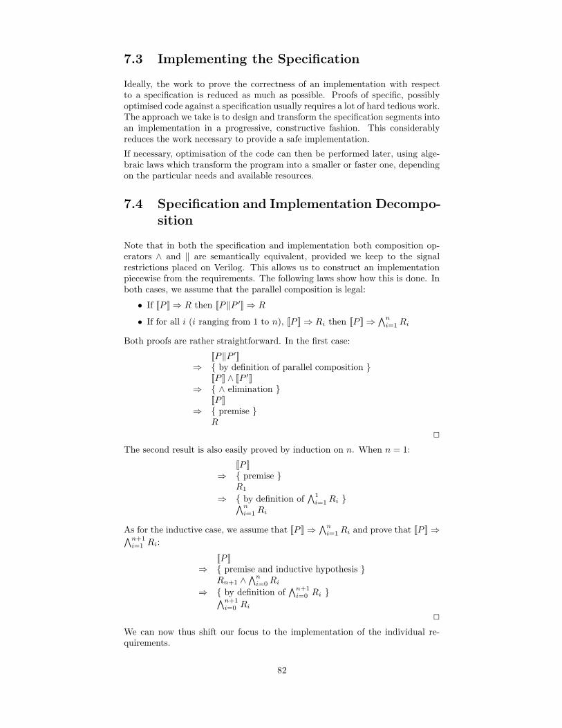
7.3 Implementing the Specification
Ideally, the work to prove the correctness of an implementation with respectto a specification is reduced as much as possible. Proofs of specific, possiblyoptimised code against a specification usually requires a lot of hard tedious work.The approach we take is to design and transform the specification segments intoan implementation in a progressive, constructive fashion. This considerablyreduces the work necessary to provide a safe implementation.
If necessary, optimisation of the code can then be performed later, using alge-braic laws which transform the program into a smaller or faster one, dependingon the particular needs and available resources.
7.4 Specification and Implementation Decompo-
sition
Note that in both the specification and implementation both composition op-erators ∧ and ‖ are semantically equivalent, provided we keep to the signalrestrictions placed on Verilog. This allows us to construct an implementationpiecewise from the requirements. The following laws show how this is done. Inboth cases, we assume that the parallel composition is legal:
• If [[P ]]⇒ R then [[P‖P ′]]⇒ R
• If for all i (i ranging from 1 to n), [[P ]]⇒ Ri then [[P ]]⇒ ∧n
i=1 Ri
Both proofs are rather straightforward. In the first case:
[[P‖P ′]]⇒ { by definition of parallel composition }
[[P ]] ∧ [[P ′]]⇒ { ∧ elimination }
[[P ]]⇒ { premise }
R
2
The second result is also easily proved by induction on n. When n = 1:
[[P ]]⇒ { premise }
R1
⇒ { by definition of∧1
i=1 Ri }∧n
i=1 Ri
As for the inductive case, we assume that [[P ]]⇒ ∧n
i=1 Ri and prove that [[P ]]⇒∧n+1
i=1 Ri:
[[P ]]⇒ { premise and inductive hypothesis }
Rn+1 ∧∧n
i=0Ri
⇒ { by definition of∧n+1
i=0 Ri }∧n+1
i=0 Ri
2
We can now thus shift our focus to the implementation of the individual re-quirements.
82

7.5 Calculation of the Implementation
7.5.1 Closing and Opening the Gate
Note that the behaviour of the closing state C ing is completely specified by
Req1 and Req10. The progress Req1 may be weakened to Aδ−→ Cing where δ ≤
15+ε. Furthermore, the requirement suggests an implementation using a delayedcontinuous assignment. The following program satisfies this requirement:
assign Cing = #δ1 A δ1 ≤ 15 + ε
Does this implementation also satisfy Req10? Firstly, we note that from theassignment assign v=#n e it immediately follows that v is stable for n timeunits. Hence, by choosing δ1 to be 4 or more, we also satisfy Req11. In fact,however, from the assign statement and assumption 2 it can be shown thatReq10 is also satisfied when δ1 < 4. We thus end up with the following programwhich satisfies Req1 and Req10:
assign Cing = #δ1 A δ1 ≤ 15 + ε
Similarly, Req4 and Req9, specifying the behaviour of Oing are satisfied by:
assign Oing = #δ2 E δ2 ≤ 15 + ε
7.5.2 The Traffic Lights
Red
The behaviour of the red light is influenced by Req3, Req5, Req7 and Req8.Since we have already seen how to implement progress requirements, we tryto construct such an implementation and then strive to satisfy the other re-quirements later. However, apparently there is a problem since the specificationprovides two, not one, progress requirements for red. This problem is solved bycombining the two Req3 and Req5 into one:
((Cing ∧ ¬C) ∨ (Oing ∧ ¬O))3+ε−→ R
Using the monotonicity of the leads to operator, it is obvious that if this re-quirement is satisfied, then so are Req3 and Req5.
Using the approach advocated in the previous section, this is implemented by:
assign Malfunction = (Cing and ∼C) or (Oing and ∼O)‖ assign R = #δ3 Malfunction δ3 ≤ 3 + ε
Note that the decomposition of the implementation into two parts is done tomake the program clearer and to avoid complications arising from situationswhere the individual variables, but not the value of the whole expression, change.
83

Yellow
The invariant conditions given in Req7 and Req8 indicate that at least one ofthe traffic lights could be implemented to be on whenever the other two are off.This immediately satisfies Req7 and part of Req8. For this we can choose eitheryellow or green (since red has already been implemented). We choose yellow,although an implementation could just as easily have been constructed if greenhad been chosen.
assign Y = ∼G and ∼R
Green
Replacing Y by ¬G∧¬R reduces Req7 to true. Requirement 8 is simply reducedto:
√(¬(G ∧R))
Also, using this replacement and replacing E by ¬A (from assumption 3), Req2and Req6 reduce to:
¬A ε−→ G ∨ RA
ε−→ ¬G ∨R
If we use an intermediate state A−, we can use monotonicity of the leads tooperator to decompose these requirements into:
¬A ε−→ ¬A−A
ε−→ A−
√(A− ⇒ (¬G ∨ R))
√(¬A− ⇒ (G ∨ R))
The first two lines are implemented by a continuous assignment:
assign A− = #δ4 A δ4 ≤ ε
Using propositional calculus transformations, it can easily be shown that ifG is replaced by ¬A− ∧ ¬R, the remaining two invariant conditions and thetransformed version of Req8 are all satisfied.
assign G = ∼A− and ∼R
This result may be reached by propositional calculus reasoning or by simplydrawing up a truth table of the invariants with the boolean states G, A−, Rand expressing G as a function of the other boolean states.
84

A
C
O
E
Cing
Oing
AG
Y
R
Figure 7.1: A circuit satisfying the real-time constraints
7.6 The Implementation
A whole family of implementations has thus been calculated from the require-ments. The whole implementation is the following:
assign Cing = #δ1 A
‖ assign Oing = #δ2 E
‖ assign Malfunction = (Cing and ∼C) or (Oing and ∼O)‖ assign R = #δ3 Malfunction
‖ assign Y = ∼G and ∼R‖ assign A− = #δ4 A
‖ assign G = ∼A− and ∼R
where the following restrictions are placed on the delays:
δ1 ≤ 15 + ε
δ2 ≤ 15 + ε
δ3 ≤ 3 + ε
δ4 ≤ ε
Thus, for example, if ε is at least 1, we can satisfy all constraints by takingδ1 = δ2 = δ3 = δ4 = 1. This implementation is shown in figure 7.1.
7.7 Other Requirements
The original specification had one other requirement: The gate must remainopen for at least 15 time units:
Req11def= S(O, 15)
Two other assumptions about the system environment were also given to providevalid implementations of the specification:
• The gate can only open when it receives an opening signal.
Ass4def= 2(d¬Oe ; dOe ⇒ true ; dOinge ; dOe)
85

• It remains open unless a closing signal is received:
Ass5def= O unless Cing
Note that the new requirement places a constraint on one of the system inputs,not outputs, and is thus not possible to prove directly as part of the construction.
Furthermore, the implementation given here does not satisfy the new require-ment and would thus require a more intelligent approach.
One possible implementation of the system would be to implement C ing moreintelligently as follows:
assign Cing = #δ1 K
‖ assign K = A∧¬OingNote that Req1 and Req10 are still satisfied using this implementation providedthat δ1 + δ2 ≤ 15 + ε.
Provided that ε ≥ 15, we can satisfy the new requirement by taking δ1 = δ2 =15. Note that a more general implementation can also be derived using lessconstructive techniques together with more intuition.
86

Chapter 8
Hardware Components
It is desirable to have a number of circuit properties from which one is able toconstruct more complex circuit specifications. This chapter gives a number ofsimple components which one may use to describe hardware. A normal form forthis specification language is identified and laws are given to transform arbitraryspecifications into this normal form. Finally, a set of laws converting normalform specifications into Verilog code are also given.
8.1 Combinational Circuits
One common property is that of having a boolean state always carrying a func-tion of a number of other states with no delay in between. This is basically acombinational circuit. Such a property is specified as follows:
C(v ←− e) def=√
(v = e)
8.2 Transport Delay
Quite frequently, it is necessary to have a signal carrying the same informationas another wire but delayed by a number of time units. This type of delay iscalled transport delay and can be specified by:
T (vδ←− e) def
=√
(v = δ � e)
8.3 Inertial Delay
A rather more complex type of delay is inertial delay. An inertially delayedsignal changes its value only after the inputs have remained constant for a givennumber of time units. We can describe this delay by:
I(v δ←− e) def=
Stable(var(e))δ−→ dv = δ � ee
∧ ¬Stable(var(e))δ−→ dv = 1� ve
where Stable(v)def= bvc ∨ b¬vc, and Stable(V )
def=∧
v∈V Stable(v).
87

Thus, if the variables in expression e remain unchanged for δ time units v takesthat value, while if any of the variables have changed value, v keeps its old value.
8.4 Weak Inertial Delay
The inertial delay behaviour, as described in the previous section can, in somecircumstances, be too strong. Usually, it is enough to ensure the positive be-haviour of the inertial delay: that the output is specified whenever the input hasremained constant for at least δ time units. The extra requirement, that when-ever the inputs have just changed, the output remains constant may be ratherdifficult to implement in certain circumstances, and may not be necessary forthe whole design. For this reason, we define a weak inertial delay:
I−(vδ←− e) def
= Stable(var(e))δ−→ dv = δ � ee
8.5 Edge Triggered Devices
An edge triggered register will output its current state, which is changed to theinput whenever a rising (or falling) edge is encountered on the trigger signal.This device will be written as ↑T |= v ←− e for input e, output v and triggersignal T . It is sensitive to a rising edge on T (a downwards arrow instead of theupwards one is used for falling edge triggered devices). To avoid feedback weassume that T is not free in e.
A delayed edge triggered device acts just like a normal edge triggered devicebut the state is changed δ units after the trigger event to the value of the input(at the trigger event). We assume that the trigger will not have more than onerising edge within δ time units of another. As before, T must not be free in e.
The formal definition of a delayed rising edge triggered device follows:
↑T |= vδ←− e def
=←−−Rise(T )
δ−→ dv = δ � ee∧ ¬←−−Rise(T )
δ−→ dv = 1� ve
where←−−Rise(T ) states that T has risen at the start of the current interval:
←−−Rise(T )
def= (de ∧←−T = false ∧ −→T = true); true.
Immediate edge triggered components can now be defined in terms of the delayedversion:
↑T |= v ←− e def= ↑T |= v
0←− e
8.6 Weak Edge Triggered Devices
As we did with the inertial delay it is sometimes sufficient to describe the be-haviour of an edge triggered device weaker than the ones introduced in theprevious section. It is usually sufficient to specify that δ time units after a trig-ger, the value of the output will change to the value of the input as it was at thetriggering event. The output will not change until another trigger is detected.
88

Note that we are weakening the specification by not determining the behaviourof the output from when the trigger is detected until δ time units later. It isusually far easier to satisfy this behaviour, and it is usually sufficient for mostbehavioural purposes. Formally, this behaviour is specified as:
↑T |=− v δ←− e def=
←−−Rise(T )
δ−→ dv = δ � ee∧ ¬←−−Rise(T ) ∧ ¬Rise(T )
δ−→ dv = 1� ve
where Rise(T )def= 3(d¬T e ; dT e).
↑T |=− v ←− e def= ↑T |=− v 0←− e
The behaviour of a weak falling edge triggered device can be similarly defined.
8.7 Hiding
Specifications are usually built hierarchically. Modules are specified in terms ofsub-modules, and the process is repeated until the resultant modules are simpleenough to specify directly. At every stage of abstraction, it is convenient to beable to hide away information which will no longer be useful at the higher levels.This is done via the hiding operator:
var vP
end v
def= ∃∃v · P
Since the hiding operator is commutative, we will extend these semantics to:
var u, . . . wP
end u, . . . w
def= ∃∃u, . . . w · P
8.8 Composition of Properties
Every component has a defined set of outputs, and a relation defining how thesignals are dependent on each other (in a combinational fashion). These aredefined in figures 8.1 and 8.2, where ∅ signifies the empty set and × is theCartesian product of two sets.
Given that two hardware properties P1 and P2 satisfy the following two condi-tions, we will be able to define their composition P1 |||P2.
Condition 1: out(P1) ∩ out(P2) = ∅
Condition 2: (dep(P1) ∪ dep(P2))+ ∩ Id = ∅
89

out(C(v ←− e)) def= {v}
out(T (vδ←− e)) def
= {v}out(I(v δ←− e)) def
= {v}out(I−(v
δ←− e)) def= {v}
out(↑T |= vδ←− e) def
= {v}out(↓T |= v
δ←− e) def= {v}
out(↑T |=− v δ←− e) def= {v}
out(↓T |=− v δ←− e) def= {v}
out(↑T |= v ←− e) def= {v}
out(↓T |= v ←− e) def= {v}
out(var v P end v)def= out(P )− {v}
Figure 8.1: The Output function
where R+ is the transitive closure of a relation, and Id is the identity functionover wires.
The first condition makes sure that no two properties control the same outputs.The second makes sure that there are no combinational loops.
We can now define the composition of two properties as follows:
P1 |||P2def= P1 ∧ P2
out(P1 |||P2)def= out(P1) ∪ out(P2)
dep(P1 |||P2)def= (dep(P1) ∪ dep(P2))
+
8.9 Algebraic Properties of Hardware Compo-
nents
A number of algebraic properties pertaining to the specification componentswill help us to prove theorems without having to fall back onto the originaldefinitions.
8.9.1 Combinational Properties
The laws of combinational properties listed here will frequently be used to splitspecifications into simpler ones.
Law AP-1 Equivalence of combinational propertiesCombinational circuits which compute equivalent propositions are themselvesequivalent.
If e = f thenC(v ←− e) = C(v ←− f) [Law – equivC]
90

dep(C(v ←− e)) def= {v} × var(e)
dep(T (vδ←− e)) def
= ∅dep(I(v δ←− e)) def
= ∅dep(I−(v
δ←− e)) def= ∅
dep(↑T |= vδ←− e) def
= ∅dep(↓T |= v
δ←− e) def= ∅
dep(↑T |=− v δ←− e) def= ∅
dep(↓T |=− v δ←− e) def= ∅
dep(↑T |= v ←− e) def= {v} × var(e)
dep(↓T |= v ←− e) def= {v} × var(e)
dep(var v P end v)def= {(u,w) ∈ dep(P ) | u 6= v ∧ w 6= v}
Figure 8.2: The dependency function
Proof:C(v ←− e)
= { by definition }√v = e
= { monotonicity of invariants and premise }√(v = e ∧ e = f)
= { monotonicity of invariants and premise }√v = f
= { by definition }C(v ←− f)
2
Law AP-2 Combinational properties and compositionCombinational equivalences can be propagated over parallel composition.
C(v ←− e) ||| Q⇒ Q[e/v] [Law – C − |||]
The proof of this law follows by induction on the structure of Q and the law ofduration calculus that: P (v) ∧ √(v = e)⇒ P (e).
8.9.2 Delay Properties
Law AP-3 Monotonicity of weak inertial delaysWeak inertial delays are refined as the delay decreases.
If ∆ ≥ δ then
I−(vδ←− e)⇒ I−(v
∆←− e) [Law – mono I−]
Proof: An outline of the proof follows:
91

I−(vδ←− e)
= { by definition }Stable(var(e))
δ−→ dv = δ � ee⇒ { monotonicity of leads to operator and ∆ ≥ δ }
Stable(var(e))∆−→ dv = δ � ee
⇒ { definition of leads to operator }2((Stable(var(e)) ∧ l = ∆); l > 0⇒ (l = ∆; dv = δ � ee)
⇒ { right hand side implies e remains constant }2((Stable(var(e)) ∧ l = ∆); l > 0⇒ (l = ∆; dv = ∆� ee)
⇒ { definition of leads to operator }Stable(var(e))
∆−→ dv = ∆� ee= { by definition }
I−(v∆←− e)
2
Law AP-4 Equivalence of delaysDelay circuits of the same type and which compute equivalent propositions arethemselves equivalent.
If e = f and var(e) = var(f) and D ∈ {T , I, I−} then
D(vδ←− e) = D(v
δ←− f) [Law – equivD]
The proof of this law follows in a similar fashion to that of Law AP-2.
Law AP-5 Weak inertial delays in sequenceWeak inertial delays can be refined by decomposing them into smaller delays insequence.
I−(zδ←− f(in′1, . . . in
′n)) ||| I−(in′i
δ′
←− ini)
⇒ I−(zδ+δ′
←− f(in1, . . . inn))[Law – I− + I− → I−]
The proof follows almost identically the one given for Law AP-3, but uses ad-
ditivity of the leads to operator: (Pn1−→ Q ∧Q n2−→ R)⇒ P
n1+n2−→ Q.
8.9.3 Edge Triggers
Law AP-6 Weak edge trigger refined by strong edge trigger and weak inertialdelayA weak edge triggered device may be decomposed into two parts: an immediatetrigger acting on the input and a weak inertial device to perform the computa-tion.
↑T |= In′ ←− In ||| I−(vδ←− f(in′1 . . . in
′n))
⇒↑T |=− v δ←− f(in1 . . . inn)[Law – weak decomp]
This law follows by reasoning similar to that of Law AP-3.
8.9.4 Composition
Law AP-7 Commutativity of compositionP ||| Q = Q ||| P [Law – comm |||]
92

Law AP-8 Associativity of composition(P ||| Q) ||| R = P ||| (Q ||| R) [Law – assoc |||]
Law AP-9 Piecewise refinement (monotonicity of composition)If P ⇒ Q and both P |||R and Q |||R are defined, then
P ||| R⇒ Q ||| R [Law – mono |||]
All three laws follow immediately from the fact that ||| is defined as conjunction(which is commutative, associative and monotonic).
8.9.5 Hiding
The laws given in this section simplify statements which use hiding. All thelaws follow from the laws of state variable quantification.
Law AP-10 Renaming hidden variablesProvided that no name clashes occur, hidden variables may be renamed freelywith no consequence on the computation performed.
Provided that v′ is not free in P :var v P end v = var v′ P [v′/v]; end v′
[Law – rename]
The proof of this law is very similar to that of Law AP-2.
Law AP-11 Moving hiding outside of propertiesThe scope of hidden variables may be increased as long as there is no nameclash.
Provided that v is not free in P :P ||| var v Q end v = var v P ||| Q end v
[Law – out var/end]
Proof:P ||| var v Q end v
= { by definition }P ∧ ∃∃v ·Q
= { v is not free in P }∃∃v · P ∧Q
= { by definition }var v P ||| Q end v
2
Law AP-12 Monotonicity of hidingRefinment may be performed within the hiding operator.
If P ⇒ Q thenvar v P end v ⇒ var v Q end v
[Law – mono var/end]
The law follows immediately from monotonicity of quantification of state vari-ables.
Law AP-13 One point ruleA hidden variable which is uniquely (and combinationally) determined can bereplaced throughout by its value.
var v P ||| C(v ←− e) end v ⇒ P [e/v] [Law – OPR]
Follows from the application of laws AP-2 and AP-12 and the fact that v is notfree in P [e/v].
93

8.10 Reducing Properties to a Normal Form
If the system complies with certain requirements, we can simplify and reducecertain properties into simpler constituent ones. The following laws can be usedto reduce an arbitrary collection of properties into a normal form. The normalform properties may then be implemented as a Verilog program.
8.10.1 The Normal Form
A property is said to be in normal form if it is a valid property and is of theform var v, . . . z P end v, . . . z, where P is a composition of the followingtypes of properties:
• Combinational circuits
• Inertial delays
• Immediate positive edge triggered registers
8.10.2 Transport to Inertial Delay
These laws will be used to convert transport delays to inertial delays which aremore readily implementable as Verilog code.
Law NF-1 Equivalence between transport and inertial delay when δ = 1Unit transport and inertial delays are interchangable.
I(v 1←− e) = T (v1←− e) [NF – T1 → I1]
Proof:I(v 1←− e)
= { by definition }Stable(var(e))
1−→ dv = 1� ee∧ ¬Stable(var(e))
1−→ dv = 1� ve= { discrete duration calculus }
true1−→ dv = 1� ee
∧ false1−→ dv = 1� ve
= { DC reasoning about leads to operator }true
1−→ dv = 1� ee= { DC reasoning }√
(v = 1� e)
= { by definition }T (v
1←− e)2
Law NF-2 Decomposition of transport delayTransport delay can be split into two delays in sequence such that the sum ofthe decomposed delays is equal to the sum of the original delay.
T (vδ1+δ2←− e) = var v′
T (vδ2←− v′) ||| T (v′
δ1←− e);end v′
[NF – decompT ]
94

This is a consequence of the law of shift: (n1 + n2)� P = n1 � (n2 � P ).
Law NF-3 Transport delay maintains stabilityThe output of a transport delayed stable variable is itself stable.
If S(var(e), n) and T (vδ←− e) then
S(v, n) [NF – stabT ]
This law follows immediately from the fact that shift maintains stability of stateexpressions.
These three laws can be reduced to just one:
Law NF-4 Transport to Inertial delayTransport delays may be decomposed into a number of sequential unit inertialdelays.
T (vδ←− e) = var t1 . . . tδ
δ
|||||||||i=0
I(ti 1←− ti+1)
end t1 . . . tδ
where t0 = v and tδ = e [NF – T → I]
8.10.3 Weak Inertial Delays
The behaviour of positive inertial delays is simulated by a transport delay.
Law NF-5 Weak Inertial to Transport delayTransport delays are a refinement of weak inertial delays.
T (vδ←− e)⇒ I−(v
δ←− e) [NF – I− → T ]
Thus follows from the law: D ⇒ (E ⇒ D).
8.10.4 Edge Triggered Registers
The laws in this section are used to reduce delayed edge triggered registers intotransport delays and immediate acting edge triggered registers. All falling edgetriggers will be converted into rising edge sensitive ones.
Law NF-6 Falling to rising edge triggers (immediate)Strong falling edge triggers can be emulated by strong rising edge triggers whichact on the negation of the original trigger.
↓T |= v ←− e = var T ′
C(T ′ ←− ¬T ) ||| ↑T ′ |= v ←− eend T ′
[NF – ↓→↑]
This is a consequence of law AP-2 and the definition of rising triggers. The nexttwo laws can also be similarly proved.
95

Law NF-7 Falling to rising edge triggers (weak)Weak falling edge triggers can be emulated by weak rising edge triggers whichact on the negation of the original trigger.
↓T |=− v δ←− e = var T ′
C(T ′ ←− ¬T ) ||| ↑T ′ |=− v δ←− eend T ′
[NF – weak ↓→↑]
Law NF-8 Falling to rising edge triggers (delayed)Delayed falling edge triggers can be emulated by delayed rising edge triggerswhich act on the negation of the original trigger.
↓T |= vδ←− e = var T ′
C(T ′ ←− ¬T ) ||| ↑T ′ |= vδ←− e
end T ′
[NF – ↓ δ→↑]
Law NF-9 Weak to strong rising edge triggered devicesStrong edge triggered devices are a refinement of weak edge triggered devices.
↑T |= vδ←− e⇒↑T |=− v δ←− e
[NF – weak-strong ↑]
This is a direct consequence of conjunction elimination: (D ∧ E)⇒ D.
Law NF-10 Remove delayed triggersDelayed triggers can be replaced by immediate triggers acting upon transportdelayed inputs and trigger signal.
↑T |= vδ←− e = var e′, T ′
T (T ′δ←− T )
||| T (e′δ←− e)
||| ↑T ′ |= v ←− e′end e′, T ′
[NF – δ → 0]
This law follows from monotonicity of invariants and the definition of rising edgetriggers.
8.11 Reduction to Normal Form
Given any property satisfying the constraints given in section 8.8, we can nowreduce it to normal form, together with a list of system requirements underwhich the normal form implies the original property. The correctness of thealgebraic laws used in the process guarantees this implication.
Using the normal form laws just given, this transformation is rather straight-forward. Throughout the following procedure, the laws about composition areused repeatedly.
96
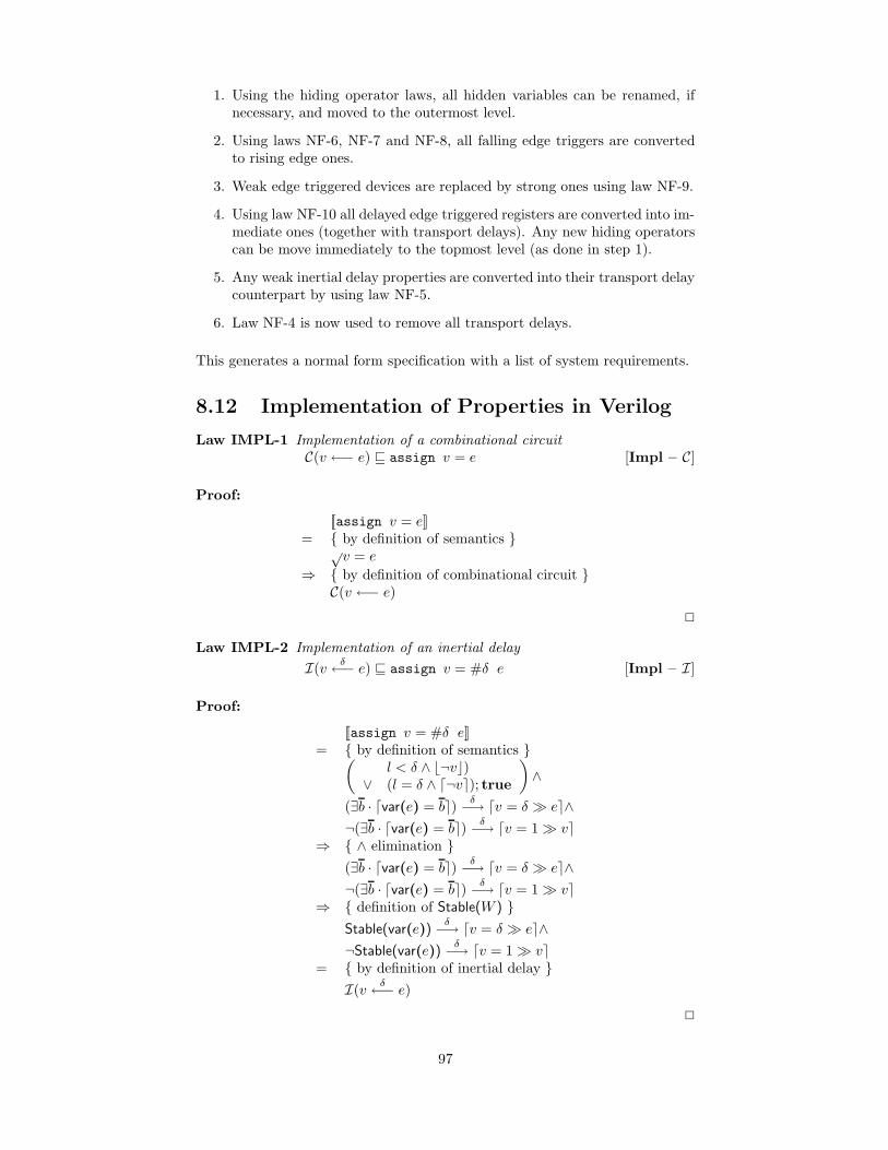
1. Using the hiding operator laws, all hidden variables can be renamed, ifnecessary, and moved to the outermost level.
2. Using laws NF-6, NF-7 and NF-8, all falling edge triggers are convertedto rising edge ones.
3. Weak edge triggered devices are replaced by strong ones using law NF-9.
4. Using law NF-10 all delayed edge triggered registers are converted into im-mediate ones (together with transport delays). Any new hiding operatorscan be move immediately to the topmost level (as done in step 1).
5. Any weak inertial delay properties are converted into their transport delaycounterpart by using law NF-5.
6. Law NF-4 is now used to remove all transport delays.
This generates a normal form specification with a list of system requirements.
8.12 Implementation of Properties in Verilog
Law IMPL-1 Implementation of a combinational circuitC(v ←− e) v assign v = e [Impl – C]
Proof:
[[assign v = e]]= { by definition of semantics }√
v = e
⇒ { by definition of combinational circuit }C(v ←− e)
2
Law IMPL-2 Implementation of an inertial delay
I(v δ←− e) v assign v = #δ e [Impl – I]
Proof:
[[assign v = #δ e]]= { by definition of semantics }
(l < δ ∧ b¬vc)
∨ (l = δ ∧ d¬ve); true
)
∧
(∃b · dvar(e) = be) δ−→ dv = δ � ee∧¬(∃b · dvar(e) = be) δ−→ dv = 1� ve
⇒ { ∧ elimination }(∃b · dvar(e) = be) δ−→ dv = δ � ee∧¬(∃b · dvar(e) = be) δ−→ dv = 1� ve
⇒ { definition of Stable(W ) }Stable(var(e))
δ−→ dv = δ � ee∧¬Stable(var(e))
δ−→ dv = 1� ve= { by definition of inertial delay }
I(v δ←− e)2
97

Law IMPL-3 Implementation of a rising edge triggered register↑T |= v ←− e v always @posedge T v = e [Impl – ↑T ]
Proof: Define LOOP as follows:
LOOPdef= µX ·
(bT c ∧ Const(v))
∨ (bT c; b¬T c ∧ ¬−→T ∧ Const(v))
∨ (bT c; d¬T e ∧ −→T ∧ Const(v)) o
9(de ∧ −→v = −→e ) o
9X
The invariant we will be working towards is:
Invdef=
(2((¬←−−Rise(T ) ∧ de)⇒←−v = −→v )∧2((←−−Rise(T ) ∧ de)⇒ −→v = −→e )
)
The following DC reasoning will be found useful later:
(−→v = −→e ∧←−−Rise(T ) ∧ de) o
9(bT c ∧ Const(v))
⇒ { relational chop and b·c definition }(−→v = −→e ∧←−−Rise(T ) ∧ de)∨(−→v = −→e ∧←−−Rise(T ) ∧ de) o
9(dT e ∧ Const(v))
⇒ { relational chop definition and DC reasoning }(−→v = −→e ∧←−−Rise(T ) ∧ de)∨(ddv = eee ∧ ←−−Rise(T )); (Const(v) ∧ 2(¬←−−Rise(T )))
⇒ { always DC clauses }Inv
Now consider the following proof outline:
(−→v = −→e ∧←−−Rise(T ) ∧ de) o
9LOOP
⇒ { recursion unfolding and above DC reasoning }Inv ∨ (l > 0 ∧ Inv); (−→v = −→e ∧←−−Rise(T ) ∧ de) o
9LOOP
⇒ { fixed point }µX · Inv ∨ (l > 0 ∧ Inv);X
⇒ { always clauses and recursion }Inv
Hence, we can deduce that:
[[always @posedge T v = e]]= { by definition of semantics }
µX ·
(bT c ∧ Const(v))
∨ (bT c; b¬T c ∧ −→T = false ∧ Const(v))
∨ (bT c; d¬T e ∧ −→T = true ∧ Const(v)) o
9(de ∧ −→v =←−e ) o
9X
= { no concurrent reading and writing and v /∈ var(e) }
µX ·
(bT c ∧ Const(v))
∨ (bT c; b¬T c ∧ ¬−→T ∧ Const(v))
∨ (bT c; d¬T e ∧ −→T ∧ Const(v)) o
9(de ∧ −→v = −→e ) o
9X
98

⇒ { recursion unfolding }
(bT c ∧ Const(v))
∨ (bT c; b¬T c ∧ ¬−→T ∧ Const(v))
∨ (bT c; d¬T e ∧ −→T ∧ Const(v)) o
9(de ∧ −→v = −→e ) o
9LOOP
⇒ { DC reasoning }Inv ∨ (Inv; (−→v = −→e ∧←−−Rise(T ) ∧ de) o
9LOOP)
⇒ { previous reasoning and always clauses in DC }Inv
⇒ { discrete DC and monotonicity of 2 and ; }2((de ∧←−−Rise(T )); l > 0⇒ dv = ee; true) ∧2((de ∧ ¬←−−Rise(T )); l > 0⇒ dv = 1� ve; true)
= { by definition of −→ }←−−Rise(T ) −→ dv = 0� ee∧¬←−−Rise(T ) −→ dv = 1� ve
= { by definition of triggered register with delay 0 }↑T |= v
0←− e= { by definition of immediate triggered register }
↑T |= v ←− e2
Law IMPL-4 Implementation of compositionIf P1 v Q1 and P2 v Q2 then
P1 |||P2 v Q1‖Q2 [Impl – |||]
Proof:
[[Q1 ‖ Q2]]= { by definition of semantics }
[[Q1]] ∧ [[Q2]]⇒ { by premise and monotonicity of ∧ }
P1 ∧ P2
= { by definition of ||| }P1 |||P2
2
8.13 Summary
This chapter shows how one can design a specification language which can bemechanically transformed into Verilog using verifiable laws. The specificationlanguage given is not particularly high level, but it is sufficient to demonstratea number of interesting uses as will be shown in the next chapter.
99

Chapter 9
Decomposition of Hardware
Component Specifications:
Examples
This chapter will specify variations on an n-bit adder using the specificationlanguage given in the previous chapter. The specifications will be modifiedand then implemented as Verilog programs using the laws of the specificationlanguage.
Three specifications of the adder are given: combinational, delayed and trig-gered:
• At the simplest level, the whole circuit may be considered as a combi-national one. The transformation becomes rather straightforward andrequires only the standard propositional calculus proof usually used toprove the correctness of an n-bit adder.
• At a higher, slightly more complex, level the individual components aregiven an inherent delay.
• Finally, a triggering signal is added to the circuit to set off the adder. Arising edge on the trigger will, after a necessary delay, produce the desiredresult on the outputs.
The main scope of this example is not simply the implementation of the givenspecification as a Verilog program. The normal form conversion laws given inchapter 8 allow us to do this automatically. Before the implementation processis carried out, we split up the specification into a number of blocks in predefinedformats. In the combinational case, for example, the specification is split up intoAND, XOR and OR gate specifications. The eventual Verilog implementationwould thus be closer to the chosen hardware components.
9.1 A Combinational n-bit Adder
The first case is a combinational circuit specification. The complete specifica-tion, for an n-bit adder can be thus described by:
100

0
Figure 9.1: The gates used: AND (∧), XOR (⊕), OR (∨), GND respectively
C-NBA-SPEC(sout, cout, a, b, n)def=
n
|||||||||i=1
C(souti ←− (
n−1∑
j=0
2j(aj + bj))!i)
||| C(cout←− (
n−1∑
j=0
2j(aj + bj))!n)
where b!i is the ith bit of bit-string b.
Note that this may be immediately synthesised into Verilog code by using law[Impl – C]. We would, however, prefer to decompose the adder into smallerpieces and perform the transformation into Verilog on the component. We usethe standard method to build an n-bit adder from n full adders, each of whichis made up of two half adders and combinational gates. The half adders arethen built directly from combinational gates. We start by showing that thisdecomposition of the circuit is in fact a correct one, and then, finally, transformthe eventual result into a Verilog program.
9.1.1 Combinational Gates
Figure 9.1 shows the different gates which will be used to build an adder. Theirsemantics are defined as follows:
C-AND(z, a, b)def= C(z ←− a ∧ b)
C-XOR(z, a, b)def= C(z ←− a⊕ b)
C-OR(z, a, b)def= C(z ←− a ∨ b)
C-GND(z)def= C(z ←− 0)
9.1.2 Half Adder
A half adder can now be defined in terms of the combinational gates. Outputc is true if and only if the inputs a and b are both true (the one bit sum of aand b leaves a carry). Output s carries the one-bit sum of a and b. Figure 9.2shows the composed circuit, which is defined as:
C-HA(s, c, a, b)def= C-XOR(s, a, b) |||C-AND(c, a, b)
101

a b
c s
Figure 9.2: The composition of a half adder
cin
a
b
s
sout
cout
AdderHalf
HalfAdder c
c
Figure 9.3: Decomposition of s full adder into half adders
9.1.3 Full Adder
A full adder can now be constructed using two half adders and a disjunction.Figure 9.3 shows how the construction is done.
C-FA(sout, cout, a, b, cin)def= var s′, c′, c′′
C-HA(s′, c′, cin, a)
||| C-HA(sout, c′′, s′, b)
||| C-OR(cout, c′, c′′)
end s′, c′, c′′
9.1.4 Correctness of the Full Adder
At this stage, we can show that the above definition of a full adder is, in fact,a correct refinement of the following specification:
C-FA-SPEC(sout, cout, a, b, cin)def= C(cout←− (a+ b+ cin) div 2)
C(sout←− (a+ b+ cin) mod 2)
Note that a, b and cin are single bits and hence this definition is not moreabstract than the specification of the n-bit adder as given in section 9.1.
The proof is rather straightforward: The definition of C-FA(sout, cout, a, b, cin)is opened up and law [Law – C − |||] is applied to s′, c′ and c′′. Using justpropositional calculus, and [Law – equivC] it can then be easily establishedthat:
C-FA(sout, cout, a, b, cin)⇒ C-FA-SPEC(sout, cout, a, b, cin)
102

ba0 0
AdderFull
sout0
cout0
. . . . . . AdderFull
a
soutn-1
coutn-1
n-1n-1 b
cout0
a1 bn-2
Figure 9.4: Decomposition of an n-bit adder into full adders
An outline of the proof follows:
C-FA(sout, cout, a, b, cin)
⇒ { definition of C-FA }var s′, c′, c′′
C(s′ ←− cin⊕ a)||| C(c′ ←− cin ∧ a)||| C(sout←− s′ ⊕ b)||| C(c′′ ←− s′ ∧ b)||| C(cout←− c′ ∨ c′′)
end s′, c′, c′′
⇒ { applying [Law – OPR] }C(sout←− (cin⊕ a)⊕ b)C(cout←− (cin ∧ a) ∨ ((cin⊕ a) ∧ b))
⇒ { using [Law – equivC] }C(cout←− (a+ b+ cin) div 2)
C(sout←− (a+ b+ cin) mod 2)
⇒ { definition of C-FA-SPEC }C-FA-SPEC(sout, cout, a, b, cin)
9.1.5 n-bit Adder
Finally, we prove, that if we connect n full adders together (as shown in figure9.4), the resultant composition implies the original specification C-NBA-SPEC.
C-NBA(sout, cout, a, b, n)def= var cin, cout0, . . . coutn−1
C-NBA′(sout, cout, a, b, n)
end cin, cout0, . . . coutn− 1
103

where C-NBA′ is defined recursively as follows:
C-NBA′(sout, cout, a, b, cin, 1)def= GND(cin)
||| C-FA(sout0, cout0, a0, b0, cin)
C-NBA′(sout, cout, a, b, cin, n+ 1)def= C-NBA(sout, cout, a, b, cin, n)
||| C-FA(soutn, coutn, an, bn, coutn−1)
Again, the proof is rather straightforward. Simply by using predicate calculusand monotonicity of combinational properties, it can be shown that the decom-position of the n-bit adder is, in fact, correct.
Theorem: C-NBA′(sout, cout, a, b, cin, n)⇒ C-NBA(sout, cout, a, b, cin, n)
Proof: The proof proceeds by induction on n. A detailed outline of the proofis presented below:
Base case: n = 1
C-NBA′(sout, cout, a, b, cin, 1)= { by definition of C-NBA′ }
GND(cin) ||| C-FA(sout0, cout0, a0, b0, cin)⇒ { result from section 9.1.4 }
GND(cin) ||| C-FA-SPEC(sout0, cout0, a0, b0, cin)= { by definition }
C(cin←− 0)||| C(cout0 ←− (a0 + b0 + cin) div 2)||| C(sout0 ←− (a0 + b0 + cin) mod 2)
⇒ { using [Law – equivC] }C(cout0 ←− (a0 + b0 + 0) div 2)
||| C(sout0 ←− (a0 + b0 + 0) mod 2)⇒ { by definition of C-NBA-SPEC }
C-NBA-SPEC(sout, cout, a, b, cin, 1)
Inductive case: n = k + 1
C-NBA′(sout, cout, a, b, cin, k+ 1)= { by definition of C-NBA′ }
C-NBA(sout, cout, a, b, cin, k)||| C-FA(soutk, coutk, ak, bk, coutk−1)
⇒ { inductive hypothesis }C-NBA-SPEC(sout, cout, a, b, cin, k)
||| C-FA(soutk, coutk, ak, bk, coutk−1)
⇒ { result from section 9.1.4 }C-NBA-SPEC(sout, cout, a, b, cin, k)
||| C-FA-SPEC(soutk, coutk, ak, bk, coutk−1)= { by definition }
k
|||||||||i=1
C(souti ←− (∑k−1
j=0 2j(aj + bj))!i)
||| C(coutk−1 ←− (∑k−1
j=0 2j(aj + bj))!k)
||| C(coutk ←− (ak + bk + coutk−1) div 2)||| C(soutk ←− (ak + bk + coutk−1) mod 2)
104

= { replacing equals for equals }k
|||||||||i=1
C(souti ←− (∑k−1
j=0 2j(aj + bj))!i)
||| C(soutk+1 ←− (∑k
j=0 2j(aj + bj))!k)
||| C(coutk−1 ←− (∑k−1
j=0 2j(aj + bj))!k)
||| C(coutk ←− (ak + bk + coutk−1) div 2)= { higher order bits do not affect lower order ones }
k
|||||||||i=1
C(souti ←− (∑k
j=0 2j(aj + bj))!i)
||| C(soutk+1 ←− (∑k
j=0 2j(aj + bj))!k)
||| C(coutk−1 ←− (∑k−1
j=0 2j(aj + bj))!k)
||| C(coutk ←− (ak + bk + coutk−1) div 2){ generalised parallel composition }
k+1
|||||||||i=1
C(souti ←− (∑k−1
j=0 2j(aj + bj))!i)
||| C(coutk−1 ←− (∑k−1
j=0 2j(aj + bj))!k)
||| C(coutk ←− (ak + bk + coutk−1) div 2)⇒ { replacing equals for equals }
k+1
|||||||||i=1
C(souti ←− (∑k
j=0 2j(aj + bj))!i)
||| C(coutk ←− (∑k
j=0 2j(aj + bj))!(k + 1))
= { by definition }C-NBA-SPEC(sout, cout, a, b, cin, k+ 1)
2
9.1.6 Implementation in Verilog
This alternative specification can be automatically implemented as a Verilogprogram using the normal form method. Again, we stress that the only reasonbecause of which this transformation was not performed on the original specifi-cation was the desire to transform the specification into a composition of partschosen from a limited set of components. This approach leads to enhanceddesign modularity.
9.2 Delayed Adder
The next step is to introduce delays within the components. Rather than justusing a combinational circuit to represent the the components, we consider gateswith inherent delays. The specification of the n-bit adder is now:
105

D-NBA-SPEC(sout, cout, a, b, n, δ)def= I−(cout
δ←− (
n−1∑
j=0
2j(aj + bj))!n)
n
|||||||||i=1
I−(soutiδ←− (
n−1∑
j=0
2j(aj + bj))!i)
Note that from the previous section this can be refined to:
D-NBA-SPEC(sout, cout, a, b, n, δ) v var sout′, cout′
C-NBA-SPEC(sout′, cout′, a, b, n)
||| I−(coutδ←− cout′)
n
|||||||||i=1
I−(sout!iδ←− sout′!i)
end sout′, cout
However, we prefer to build the adder from delayed gates for a deeper study ofdelays.
9.2.1 The Logic Gates
A number of logic gates with an inherent delay are defined.
D-AND(z, a, b, δ)def= I−(z
δ←− a ∧ b)D-XOR(z, a, b, δ)
def= I−(z
δ←− a⊕ b)D-OR(z, a, b, δ)
def= I−(z
δ←− a ∨ b)
9.2.2 Half Adder
A half adder can now be constructed using the gates just defined. To simplifyslightly the presentation, we take both gates in the half adder to have the samedelay δ.
D-HA(s, c, a, b, δ)def= D-XOR(s, a, b, δ)
||| D-AND(c, a, b, δ)
9.2.3 Full Adder
We can now construct a full adder by using two half adders and an OR gate. Forsimplicity, we take both half adders and the disjunction gate to have the samedelay δ.
106

D-FA(s, cout, a, b, cin, δ)def= var s′, c′, c′′
D-HA(s′, c′, a, b, δ)
||| D-HA(s, c′′, s′, cin, δ)
||| D-OR(cout, c′, c′′, δ)
end s′, c′, c′′
9.2.4 Proof of Correctness
The specification of the full adder is modified for the new situation. Due tothe reaction time of the gates, we cannot be as optimistic about the circuitbehaviour as we were in the previous case. However, it will be enough for ahardware engineer to be guaranteed that if the inputs remain stable for longenough, the right result will finally appear on the output wires.
D-FA-SPEC(sout, cout, a, b, cin, δ)def= I−(cout
δ←− (a+ b+ cin) div 2)
||| I−(soutδ←− (a+ b+ cin) mod 2)
We now claim that:
D-FA-SPEC(sout, cout, a, b, cin,∆) v D-FA(sout, cout, a, b, cin, δ)
provided that ∆ ≥ 3δ. This stability requirement is usually easy to fulfill, sincewe would normally only allow changes on the global signals at a clock signal,whose period would be much larger than the propagation delay within a logicgate.
The proof of this claim is expounded below:
D-FA(sout, cout, a, b, cin, δ)
⇒ { definition of D-FA }var s′, c′, c′′
I−(s′δ←− cin⊕ a)
||| I−(c′δ←− cin ∧ a)
||| I−(soutδ←− s′ ⊕ b)
||| I−(c′′δ←− s′ ∧ b)
||| I−(coutδ←− c′ ∨ c′′)
end s′, c′, c′′
⇒ { applying [Law – I− + I− → I−] }var s′, c′, c′′
I−(sout2δ←− (cin⊕ a)⊕ b)
||| I−(cout3δ←− (cin ∧ a) ∨ ((cin⊕ a) ∧ b))
end s′, c′, c′′
⇒ { applying [Law – mono I−] }
107

I−(sout∆←− (cin⊕ a)⊕ b)
||| I−(cout∆←− (cin ∧ a) ∨ ((cin⊕ a) ∧ b))
⇒ { applying [Law – equiv D] }
I−(sout∆←− (a+ b+ c) mod 2)
||| I−(cout∆←− (a+ b+ c) div 2)
⇒ { by definition of D-FA-SPEC }D-FA-SPEC(sout, cout, a, b, cin,∆)
9.2.5 n-bit Delayed Adder
An n-bit adder can now be constructed from these components. The implemen-tation is identical to the one in section 9.1.5 except that delayed full adders areused. If full adders constructed from δ delay half adders are used, the imple-mentation will guarantee the following specification:
D-NBA-SPEC(sout, cout, a, b, n,∆) v D-NBA(sout, cout, a, b, n, δ)
provided that the ∆ ≥ 3nδ.
The proof is similar to the proof of the correctness of the full adder decomposi-tion.
9.2.6 Implementation in Verilog
By transforming D-NBA into normal form and implementing in Verilog, we auto-matically have an implementation of D-NBA-SPEC(sout, cout, a, b, n,∆). Need-less to say, we must ensure that the proof obligations arising from the transfor-mation are satisfied for the non-input wires. This is easily shown to be satisfiedif the inputs remain constant for longer than the δ inherent delay of implemen-tation of the n-bit adder. The resultant Verilog program is shown below:
D-NBA-VERILOG(sout, cout, a, b, δ, n)def=
assign cin = 0‖ D-FA-VERILOG(soutp, cout0, a0, b0, cin)
‖...
‖ D-FA-VERILOG(soutn−1, cout, an−1, bn−1, coutn−1)
where the full adder implementation is:
D-FA-VERILOG(sout, cout, a, b, cin, δ)def=
var cin
assign s′ = #δ a⊕ b
‖ assign c′ = #δ a ∧ b
‖ assign sout = #δ s′ ⊕ cin
‖ assign c′′ = #δ s
′ ∧ cin
‖ assign cout = #δ c′ ∨ c
′′
end cin
108

9.3 Triggered Adder
Finally, we add a triggering signal T to the adder. δ time units after a risingedge on the trigger the output represents the sum of the inputs at the time ofthe trigger.
The specification of this device is rather straightforward:
T-NBA-SPEC(sout, cout, a, b, δ, n)def=
n
|||||||||i=1
↑T |=− souti δ←− (∑n−1
j=0 2j(aj + bj))!i
||| ↑T |=− cout δ←− (∑n−1
j=0 2j(aj + bj))!n
9.3.1 Components
We now need another new basic component, a triggered register. Basically,such a register changes its state to the current value of the input whenever atriggering event occurs.
T-REG(T, z, a)def= ↑T |= z ←− a
9.3.2 Decomposition of the Specification
Using the implementation of a delayed n-bit adder, we can now easily obtain areasonable decomposition of the specification.
n
|||||||||i=1
T-REG(T, a′!i, a!i)
n
|||||||||i=1
T-REG(T, b′!i, b!i)
||| D-NBA(sout, cout, a′, b′, n, δ)
⇒ { definition of T-REG and correctness of D-NBA }n
|||||||||i=1
↑T |= a′i ←− ai
n
|||||||||i=1
↑T |= a′i ←− ai
n
|||||||||i=1
I−(soutiδ←− (
∑n−1j=0 2j(a′j + b′j))!i)
||| I−(coutδ←− (
∑n−1j=0 2j(a′j + b′j))!n)
⇒ { using [Law – weak decomp] }
109

n
|||||||||i=1
↑T |=− souti δ←− (∑n−1
j=0 2j(aj + bj))!i
||| ↑T |=− cout δ←− (∑n−1
j=0 2j(aj + bj))!n
⇒ { definition of T-NBA-SPEC }T-NBA-SPEC(sout, cout, a, b, δ, n)
9.3.3 Implementation
The specification, which we have just transformed into logical blocks can nowbe automatically translated into Verilog:
T-NBA-SPEC(sout, cout, a, b, δ, n) v T-NBA-VERILOG(sout, cout, a, b, δ, n)
where T-NBA-VERILOG(sout, cout, a, b, δ, n) is the following Verilog program:
T-NBA-VERILOG(sout, cout, a, b, δ, n)def= always @posedge T a
′ = a
‖ always @posedge T b′ = b
‖ D-NBA-VERILOG(sout, cout, a, b, δ, n)
9.4 Conclusions
This chapter shows how the automatic normal form transformation from cir-cuit specifications into Verilog does not need to be done immediately on thespecification. System modularity is achieved by using only a limited number ofcomponents. The algebraic laws which are used, are usually sufficient to com-bine a number of different delayed circuit properties into a single one. Hence,the n-bit adder can be just as easily included in another design as the gateswere used in the full adder or the full adder in the n-bit adder. Since the lawsare always applied in the same fashion, this process may be (at least, partially)mechanically done, which reduces tedious work and human errors. A similarapproach to triggered components may be used to decompose the n-bit trig-gered adder into triggered full adders and the same approach would then beapplicable to design a circuit which uses n-bit adders.
The main restriction of the specification language which may seem to be, atfirst sight, far too restrictive is the fact that combinational circuits with feed-back are not allowed. This has been done so as to avoid certain problems suchas short circuits (for example C(v ←− ¬v)). On the other hand, one may ar-gue that feedback is essential to build memory devices and is thus desirable.Various approaches have been proposed in the literature to deal with this prob-lem [Hoa90, Win86, Her88], most of which use sophisticated models to predictsuch behaviour. With these models it is usually then possible to verify thebehaviour of a small number of devices which, when combined together undercertain restrictions (not unlike the ones placed in our language), their behaviourcan be described using a simpler description. The approach taken here was tointroduce memory devices as primitives, thus bypassing the problem altogether.
110

However note that we cannot decompose the memory devices any further withinour model.
Thanks to the restricted specification language, the transformation of circuitproperties into separate components can be handled rather easily at the speci-fication level. This allows the generation of a Verilog program which uses onlycertain components. An alternative approach would be to have a number oflaws to transform a Verilog program into a better structured one. Due to thegenerality of Verilog programs, this would have been much more difficult thanthe approach taken here.
111

Part IV
The use of the formal semantics of language isnot restricted to proving programs correct withrespect to a specification. In this final part weconsider two other aspects — we prove the cor-rectness of a compilation procedure from Verilogto hardware and show that a simple simulationsemantics is equivalent to the denotational se-mantics already defined.
112

Chapter 10
A Hardware Compiler for
Verilog
10.1 Introduction
Verilog instructions can be rather neatly classified into two types: imperativeprogramming style instructions such as sequential composition and loops, andmore hardware oriented instructions such as continuous assignments. Designof a product usually starts by writing a behavioural module which solves theproblem. This is, however, not directly implementable as hardware and has to berefined to produce modules which can be synthesised to hardware. Refinementis usually a rather ad hoc procedure where parts of the solution are proposedand their output compared to that of the behavioural description via simulation.The behavioural program is thus taken to be the specification of the product.
Various problems can be identified in this refinement process.
• The base case: the behavioural description of the problem is not guaran-teed to be correct. The ‘correctness’ of the ‘specification’ (with respect tothe desired product) is usually checked via a number of simulation runson different inputs. This process is dangerous enough in a sequential pro-gramming environment, let alone in a language like Verilog, where newdangers introduced by parallel interleaving and the nature of most hard-ware products to continuously sample the inputs (as opposed to beinggiven a number of inputs at the beginning of the run of a program). Onemay argue that a mathematical description of the requirements still suf-fers from the same problem. However, mathematics is a far more abstractand powerful means of describing expectations and is thus considerablyless susceptible to this kind of error.
• The refinement steps: As already noted elsewhere, simulation can onlyidentify the presence of errors and not their absence. Nothing short ofexhaustive simulation can guarantee correctness.
The first problem can be solved by formally verifying the correctness of an im-perative behavioural description with respect to a more abstract mathematicalspecification. The second problem may also be solved in a similar fashion. In-deed, one may choose to verify directly the correctness of the final product.However, the closer we get to the lowest level implementation, the more diffi-cult and tedious the proofs become. This problem can be solved in a different
113

fashion: by formally proving the correctness of a compilation process from im-perative programs down to hardware-like programs.
In the approach presented here, the compilation procedure performs no prepro-cessing on the input program. This contrasts with commercial synthesis tools[Pal96, SSMT93], which perform certain transformations to help synthesize codewhich would otherwise be impossible to convert to hardware in a meaningfulmanner. For example, consider the following program:
always @clk v=¬v; w=v; v=¬v;Clearly, unless v keeps the temporary value (the negation of its original value)for an amount of time, w could never manage to read that value. However, onthe other hand, if the spike on v take any time at all, it may violate timingconstraints satisfied by the above code portion. The solution is to collapse theassignments into a single parallel assignment:
always @clk v,w=v,¬v;Note that in our case, this kind of transformations would have to be performedmanually, before the compilation procedure is performed.
The approach used here is very similar to [HJ94, Pag93, May90]. We compareour work with their approach in more detail in section 10.5.4.
10.2 Triggered Imperative Programs
We will not be dealing with all programs, but only ones which are triggeredby a start signal and upon termination issue a finish signal. The environmentis assumed not to interfere with the program by issuing a further start signalbefore the program has terminated.
Triggered programs can be constructed from general imperative programs:
ψfs (P )
def= forever (s?; P ; f !)
At the topmost level, these programs also ensure that the termination signal isinitialised to zero:
iψfs (P )
def= initial f = 0; ψf
s (P )
The environment constraint for two signals s and f may now be easily expressed:
εfs w forever ( s!; #1; f?; ∆0)
where ∆0 is a statement which, once triggered, waits for an arbitrary length oftime (possibly zero or infinite) before allowing execution to resume.
[[∆0]]W (D)def= Const(W ) ∨ Const(W ) o
9D
The unit delay ensures that if a start signal is sent immediately upon receivinga finish signal, we do not interpret the old finish signal as another finish signal.
114

Now, we ensure that if we start off with a non-zero delay, the start signal isinitially off:
iεfs w ((¬s>; ∆) u skip) ; εfs
∆ is a statement almost identical to ∆0 but which, once triggered, waits for anon-zero arbitrary length of time (possibly infinite) before allowing executionto resume.
P w Q, read as ‘P is a refinement of Q,’ is defined as P ⇒ Q.
[[∆]]W (D)def= Const(W ) ∨ (l > 0 ∧ Const(W )) o
9D
∆ obeys a number of laws which we will find useful:
skip and delay: ∆0 = skip u ∆
dur(P ) and delay: If dur(P ), then ∆ v P 1.
Signals and delay: If a variable is a signal (recall definition of signals fromchapter 6), then its behaviour is a refinement of:
(skip u ¬s>; ∆); forever s!; ∆
The results which follow usually state a refinement which holds if a particularenvironment condition holds. Hence, these are of the form:
environment condition ⇒ (P ⇒ Q)
To avoid confusion with nested implications, we define the conditional refine-ment iεfs ` P v Q as follows:
iεfs ` P v Qdef= ` iεfs ⇒ (Q⇒ P )
We can now use this to specify equality of processes under a particular environ-ment condition:
iεfs ` P = Qdef= (iεfs ` P v Q) ∧ (iεfs ` Q v P )
The following proofs assume that all programs (and sub-programs) satisfy dur(P )(hence programs take time to execute). Note that if P and Q satisfy this con-straint, so do P ;Q, P / b . Q and P ∗ b.Since we will be replacing sequential composition by parallel composition, writ-ing to a variable and then reading immediately after can cause problems. Wethus add the constraint that programs do not read or write as soon as they aexecuted (P = Q;R such that Q does not read or write data. Again, note that ifall primitive programs satisfy this condition, so do programs constructed usingsequential composition, conditionals and loops.
1This has a similar type problem as we had with the law P v P ‖ Q. A similar approach,using chaos can, however, resolve the problem.
115

10.3 The Main Results
10.3.1 Sequential Composition
Theorem 1.1: Sequential composition can be thus decomposed:
iεfs ` iψfs (P ;Q) v iψm
s (P ′) ‖ iψfm(Q′) ‖ Merge
where for any program P , we will use P ′ to represent P [vP /v]. Merge has beendefined in section 6.12.
Proof: First note the following result:
iεfs ‖ ψfs (P ;Q)
= { communication laws }(¬s>; ∆ u skip); s!;P ;Q; f !; ∆0; (ε
fs ‖ ψf
s (P ;Q))
= { by law of ∆0 }(¬s>; ∆ u skip); s!;P ;Q; f !; (¬s>; ∆ u skip); (εfs ‖ ψf
s (P ;Q))
= { by definition of iε }(¬s>; ∆ u skip); s!;P ;Q; f !; (iεfs ‖ ψf
s (P ;Q))
= { definition of forever }forever (¬s>; ∆ u skip); s!;P ;Q; f !
v { new signal introduction and laws of signals }forever ¬m>; (¬s>; ∆ u skip); s!;P ;m!;Q; f !
Now consider the other side of the refinement:
iεfs ‖ iψms (P ′) ‖ ψf
m(Q′)
= { communication laws }¬m>; (¬s>; ∆ u skip);P ′;m!;Q′; f !;¬m>; ∆0; (ε
fs ‖ ψm
s (P ′) ‖ ψfm(Q′))
= { definition of iε, iψ and law of ∆0 }¬m>; (¬s>; ∆ u skip);P ′;m!;Q′; f !; (iεfs ‖ iψm
s (P ′) ‖ ψfm(Q′))
= { definition of forever }forever ¬m>; (¬s>; ∆ u skip);P ′;m!;Q′; f !
We can now prove the desired refinement:
iεfs ‖ iψfs (P ;Q)
v { definition of iψ and proved inequality }¬f>; forever ¬m>; (¬s>; ∆ u skip); s!;P ;m!;Q; f !
= { laws of merge from section 6.12 }Merge ‖ (¬f>; forever ¬m>; (¬s>; ∆ u skip); s!;P ′;m!;Q′; f !)
= { above claim }Merge ‖ (¬f>; (iεfs ‖ iψm
s (P ′) ‖ ψfm(Q′))
= { definition of iψ and associativity of ‖ }Merge ‖ iεfs ‖ iψm
s (P ′) ‖ iψfm(Q′)
2
116

10.3.2 Conditional
Theorem 1.2: Conditional statements can be thus decomposed:
εfs ` ψfs (P / b . Q) v ψfP
sP(P ′) ‖ ψfQ
sQ(Q′) ‖ Merge ‖ Interface
where
Interface = assign sP = s ∧ b ‖assign sQ = s ∧ ¬b ‖assign f = fP ∨ fQ
Proof: Again the proof proceeds by first proving two properties and then com-bining the results to complete the theorem.
Result 1
iεfs ‖ ψfP
sP(P ′) ‖ ψfQ
sQ(Q′) ‖ Interface
= { communication laws }(¬s>;¬s>P ;¬s>Q; ∆ u skip); s!;
(f?; εfs ‖ ψfP
sP(P ′) ‖ ψfQ
sQ(Q′) ‖ Interface)
= { communication laws }(¬s>;¬s>P ;¬s>Q; ∆ u skip); s!; (sP !;P ′; fP !) / b . (sQ!;Q′; fQ!);
(¬s>; ∆ u skip); (εfs ‖ ψfP
sP(P ′) ‖ ψfQ
sQ(Q′) ‖ Interface)
= { definition of loops }forever (¬s>;¬s>P ;¬s>Q; ∆ u skip); s!; (sP !;P ′; fP !) / b . (sQ!;Q′; fQ!)
w { variable hiding }forever (¬s>; ∆ u skip); s!;P ′ / b . Q′; f !
Result 2: This result is just stated. The proof can be rather easily constructedusing the communication laws.
iεfs ‖ ψfs (P / b . Q) = forever (¬s>; ∆ u skip); s!;P / b . Q; f !
Finally, we combine the two results to complete the desired proof.
iεfs ‖ iψfs (P / b . Q)
= { result 2 }(¬f>; ∆ u skip); forever (¬s>; ∆ u skip); s!;P / b . Q; f !
v { merge laws }Merge ‖ (¬f>; ∆ u skip); forever (¬s>; ∆ u skip); s!;P ′ / b . Q′; f !
v { result 1 }(¬f>; ∆ u skip); (iεfs ‖ ψfP
sP(P ′) ‖ ψfQ
sQ(Q′) ‖ Interface ‖ Merge)
v { definition of iε }iεfs ‖ iψfP
sP(P ′) ‖ iψfQ
sQ(Q′) ‖ Interface ‖ Merge
2
117

10.3.3 Loops
Theorem 1.3: Loops can be decomposed into their constituent parts.
εfs ` ψfs (P ∗ b) v ψfP
sP(P ) ‖ Interface
where
Interface = assign sP = s ∨ (fP ∧ b) ‖assign f = fP ∧ ¬b
Proof: First of all, we note that:
¬f>; sP !; (ψfPsP
(P ) ‖ f?; ∆0; εfs ‖ Interface)
= ¬f>; (sP !;P ; fP !) ∗ b; f !; (iεfs ‖ ψfP
sP(P ) ‖ Interface)
The outline of the proof is given below. Let us refer to the left hand side of theequality as α:
α
= ¬f>; sP !; (ψfPsP
(P ) ‖ f?; ∆0; εfs ‖ Interface)
= { laws of communication and loops }¬f>; sP !;P ; fP !;α / b . (f !; (iεfs ‖ ψfP
sP(P ) ‖ Interface))
= { laws of loops }¬f>; (sP !;P ; fP !) ∗ b; f !; (iεfs ‖ ψfP
sP(P ) ‖ Interface)
This can now be used in the main proof of the theorem. The theorem is provedby showing that:
iεfs ‖ ψfs (P ∗ b) v iεfs ‖ ψfP
sP‖ Interface
The desired result would then follow immediately.
This inequality is proved as follows:
{ RHS (right hand side of inequality) }= iεfs ‖ ψfP
sP‖ Interface
= { by communication laws }(¬s>;¬s>P ; ∆ u skip); s!; sP !;P ; fP !;α / b . (f !; RHS)
= { by the result just given }(¬s>;¬s>P ; ∆ u skip); s!; sP !;P ; fP !;
(¬f>; (sP !;P ; fP !) ∗ b; f !; RHS) / b . (f !; RHS)
= { by distribution of sequential composition in conditionals }(¬s>;¬s>P ; ∆ u skip); s!; sP !;P ; fP !; ((sP !;P ; fP !) ∗ b; /b . skip); f !; RHS
= { law of loops }
118

(¬s>;¬s>P ; ∆ u skip); s!; (sP !;P ; fP !) ∗ b; f !; RHS
= { definition of forever loops }forever (¬s>;¬s>P ; ∆ u skip); s!; (sP !;P ; fP !) ∗ b; f !
w { hiding variables }forever (¬s>; ∆ u skip); s!;P ∗ b; f !
But, on the other hand:
iεfs ‖ ψfs (P ∗ b)
= { communication laws }(¬s>; ∆ u skip); s!;P ∗ b; f !; (iεfs ‖ ψf
s (P ∗ b))= { definition of loops }
forever (¬s>; ∆ u skip); s!;P ∗ b; f !
2
10.4 Compilation
Using these refinements, we can now define a compilation process:
Ψfs (P ;Q)
def= Ψm
s (P ) ‖ Ψfm(Q) ‖ Merge
Ψfs (P / b . Q)
def= ΨfP
sP(P ′) ‖ ΨfQ
sQ(Q′) ‖ Merge ‖ InterfaceC
Ψfs (P ∗ b) def
= ΨfP
sP(P ) ‖ InterfaceL
Ψfs (P )
def= ψf
s (P ) otherwise
We know that the individual steps of the compilation process are correct. How-ever, it is not yet clear whether the environment conditions can flow throughthe compilation. In other words, when we split sequential composition intotwo parts, we showed that the environment conditions for both processes wasguaranteed. But is this still the case if we refine the processes further?
Lemma 2.1: Provided that s and f are signals, if∫f ≤
∫s � 1 and
∫f ≤
∫s ≤
∫f + 0.5 are valid duration formula, then so is iεfs .
Proof: Since the inequality holds for all prefix time intervals, and s and f areboth signals, we can use duration calculus reasoning to conclude that:
2((dse ∧ l = 0.5); true; (dse ∧ l = 0.5)⇒ l = 1; true; dfe; true)
This allows us to deduce that s!; ∆; s!; ∆⇒ s!; #1; f?; ∆0; s!; ∆.
But s is a signal, and hence satisfies (¬s>; ∆ u skip); forever s!; ∆.
forever s!; ∆
= { definition of forever loops }s!; ∆; s!; ∆; forever s!; ∆
⇒ { by implication just given }s!; #1; f?; ∆0; s!; ∆; forever s!; ∆
119

= { definition of forever loops }s!; #1; f?; ∆0; forever s!; ∆
⇒ { definition of forever loops }forever s!; #1; f?; ∆0
Hence, from the fact that s is a signal, we can conclude the desired result:
(¬s>; ∆ u skip); forever s!; ∆⇒ (¬s>; ∆ u skip); forever s!; #1; f?; ∆0
= iεfs
2
Lemma 2.2: iεfs ⇒∫s ≤
∫f + 0.5.
Proof: The proof of this lemma follows by induction on the number of timesthat the environment loop is performed. We first note that iεfs can be rewrittenas:
(¬s>; ∆ u skip); s!; #1; forever (f?; ∆0; s!; #1)
Using the law f? = f> u (¬f>; #1; f?) and distributivity of non-deterministicchoice, it can be shown that this program is equivalent to:
(¬s>; ∆ u skip); s!; #1; forever
f>; s!; #1u f>; ∆; s!; #1u ¬f>; #1; f?; ∆0; s!; #1
Using the laws of loops this is equivalent to:
(¬s>; ∆ u skip); s!; #1; forever
f>; s!; #1u ¬s>; f>; ∆; s!; #1u ¬s>;¬f>; #1; f?; ∆0; s!; #1
The semantic interpretation of this program takes the form:P ′ ∨ ∃n : � · P ;Qn;Q′
where P ′ corresponds to the partial execution of (¬s>; ∆uskip); s!; #1, and Pto its full execution. Similarly, Q′ and Q correspond to the partial and completeexecution of the loop body.
P ⇒ b¬sc; (dse ∧ l = 0.5); b¬scQ ⇒ (true; dfe; true ∧ b¬sc; (dse ∧ l = 0.5)); b¬scP ′ ⇒ b¬sc ∨ b¬sc; (dse ∧ l = 0.5); b¬scQ′ ⇒ b¬sc ∨ (b¬sc; (dse ∧ l = 0.5); b¬sc ∧ true; dfe; true)
Since P ′ ⇒∫s = 0.5, it immediately follows that P ′ ⇒
∫s ≤
∫f + 0.5.
We can also show, by induction on n, that P ;Qn implies this invariant. Anoutline of the inductive case is given below:
P ;Qn+1
= P ;Qn;Q
⇒ (∫s ≤
∫f + 0.5);Q
⇒ (∫s ≤
∫f + 0.5); (
∫s = 0.5 ∧
∫f ≥ 0.5)
⇒∫s ≤
∫f + 0.5
120

Finally, we can use this result to show P ;Qn;Q′ ⇒∫s ≤
∫f + 0.5.
P ;Qn;Q′
⇒ (∫s ≤
∫f + 0.5);Q′
⇒ (∫s ≤
∫f + 0.5);
∫s = 0 ∨
(∫s ≤
∫f + 0.5); (
∫s = 0.5 ∧
∫f ≥ 0.5)
⇒∫s ≤
∫f + 0.5
This completes the required proof.2
Lemma 2.3: Provided that dur(P ):iψf
s (P )⇒∫f ≤
∫s ∧
∫f ≤
∫s� 1
Proof: Note that iψfs (P ) is a refinement of (¬f>; ∆ u skip); forever f !; s?; ∆
which is almost identical to iεsf .
The proof follows almost identically to that of lemma 2.2 except that, unlikethe environment condition, iψf
s (P ) cannot signal on f as soon as it receives asignal on s (since P must take some time to execute). This allows us to gainthat extra 0.5 time unit.
2
Lemma 2.4: The environment conditions follow along the compilation process:
Ψfs (P )⇒
∫f ≤
∫s
Proof: The proof uses structural induction on the program:
In the base case, P cannot be decomposed any further, and hence Ψfs (P ) =
ψfs (P ). Therefore, by lemma 2.3, we can conclude that
∫f ≤
∫s.
Inductive case: We proceed by considering the three possible cases: P = Q;R,P = Q / b . R and P = Q ∗ b.
Sequential composition: P = Q;R
Ψfs (P )
= { by definition of Ψ }Ψm
s (Q) ‖ Ψfm(R)
⇒ { by inductive hypothesis }∫f ≤
∫m ∧
∫m ≤
∫s
⇒ { ≤ is transitive }∫f ≤
∫s
Conditional: P = Q / b . R
Ψfs (P )
= { by definition of Ψ }ΨfQ
sQ(Q) ‖ ΨfR
sR(R) ‖ InterfaceC
121

⇒ { by inductive hypothesis }∫fQ ≤
∫sQ ∧
∫fR ≤
∫sR ∧ InterfaceC
⇒ { by definition of InterfaceC }∫fQ ≤
∫sQ ∧
∫fR ≤
∫sR ∧
∫sQ +
∫sR =
∫s ∧
∫f =
∫fQ +
∫fR −
∫(fQ ∧ fR)
⇒ { by properties of ≤ and∫}
∫f ≤
∫s
Loops: P = Q ∗ b
Ψfs (P )
= { by definition of Ψ }ΨfQ
sQ(Q) ‖ InterfaceL
⇒ { by inductive hypothesis }∫fQ ≤
∫sQ ∧ InterfaceL
⇒ { by definition of InterfaceL and integral reasoning }∫fQ ≤
∫sQ ∧
∫f =
∫s− (
∫sQ −
∫fQ)−
∫(fQ ∧ b ∧ s)
⇒ { by properties of ≤ }∫f ≤
∫s
This completes the inductive step and hence the result holds by induction.2
Lemma 2.5: Ψfs (P )⇒
∫f ≤
∫s� 1
Proof: The proof follows almost identically to that of lemma 2.4.2
Theorem 2: If s is a signal, then:∫s ≤
∫f + 0.5 ` ψf
s (P ) v Ψfs (P )
Proof: The proof follows by induction on the structure of the program P .
In the base case, when P is a simple program, Ψfs (P ) is just ψf
s (P ), and hencetrivially guarantees correctness.
For the inductive case we consider the different possibilities:
Sequential composition: We need to prove that∫s ≤
∫f+0.5 ` ψf
s (Q;R) vΨf
s (Q;R)
Assume that∫s ≤
∫f + 0.5.
By lemma 2.4, Ψfs (Q;R) guarantees that
∫f ≤
∫s and hence:
∫f ≤
∫s ≤
∫f + 0.5
But, by definition of Ψ, and the further application of lemma 2.4:
122

Ψms (Q′) ‖ Ψf
m(R′)∫m ≤
∫s
∫f ≤
∫m
Hence, combining the above inequalities with the previous ones:
∫m ≤
∫f + 0.5
∫s ≤
∫m+ 0.5
By the inductive hypothesis, we thus conclude that:
ψms (Q′) ‖ ψf
m(R′)
Also, by lemma 2.5 we can conclude that∫f ≤
∫s � 1. This, together
with the first inequality allows us to apply lemma 2.1, implying that iεfs .Thus we can apply theorem 1.1 to conclude that ψf
s (Q;R).
Therefore,∫s ≤
∫f + 0.5 ` ψf
s (P ;Q) v Ψfs (P ;Q).
Conditional: We need to prove that:∫s ≤
∫f + 0.5 ` ψf
s (Q / b . R) v Ψfs (Q / b . R)
As before, we know that:
∫f ≤
∫s ≤
∫f + 0.5
Also, by definition of Ψ and lemma 2.4:
ΨfQsQ
(Q) ‖ ΨfRsR
(R) ‖ InterfaceC∫fR ≤
∫sQ
∫fR ≤
∫sR
Using simple duration calculus arguments on the interface part, we canconclude that:
∫s =
∫sQ +
∫sR
∫f =
∫fQ +
∫fR −
∫(fQ ∧ fR)
123
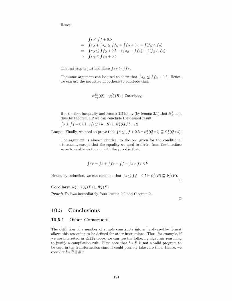
Hence:
∫s ≤
∫f + 0.5
⇒∫sQ +
∫sR ≤
∫fQ +
∫fR + 0.5−
∫(fQ ∧ fR)
⇒∫sQ ≤
∫fQ + 0.5− (
∫sR −
∫fR)−
∫(fQ ∧ fR)
⇒∫sQ ≤
∫fQ + 0.5
The last step is justified since∫sR ≥
∫fR.
The same argument can be used to show that∫sR ≤
∫fR + 0.5. Hence,
we can use the inductive hypothesis to conclude that:
ψfQ
sQ(Q) ‖ ψfR
sR(R) ‖ InterfaceC
But the first inequality and lemma 2.5 imply (by lemma 2.1) that iεfs , andthus by theorem 1.2 we can conclude the desired result:∫s ≤
∫f + 0.5 ` ψf
s (Q / b . R) v Ψfs (Q / b . R).
Loops: Finally, we need to prove that∫s ≤
∫f + 0.5 ` ψf
s (Q ∗ b) v Ψfs (Q ∗ b).
The argument is almost identical to the one given for the conditionalstatement, except that the equality we need to derive from the interfaceso as to enable us to complete the proof is that:
∫sP =
∫s+
∫fP −
∫f −
∫s ∧ fP ∧ b
Hence, by induction, we can conclude that∫s ≤
∫f + 0.5 ` ψf
s (P ) v Ψfs (P ).
2
Corollary: iεfs ` iψfs (P ) v Ψf
s (P ).
Proof: Follows immediately from lemma 2.2 and theorem 2.2
10.5 Conclusions
10.5.1 Other Constructs
The definition of a number of simple constructs into a hardware-like formatallows this reasoning to be defined for other instructions. Thus, for example, ifwe are interested in while loops, we can use the following algebraic reasoningto justify a compilation rule. First note that b ∗ P is not a valid program tobe used in the transformation since it could possibly take zero time. Hence, weconsider b ∗ P ‖ #1:
124

b ∗ P ‖ #1
= { definition of while loops }((P ; b ∗ P ) / b . skip) ‖ #1
= { distribution of parallel composition into conditional }(P ; b ∗ P ‖ #1) / b . (skip ‖ #1)
= { laws of #1 with parallel composition and dur(P ) }(P ; b ∗ P ) / b .#1
= { by definition of repeat loops }(P ∗ b) / b .#1
Hence, by monotonicity, ψfs (b ∗ P ‖ #1) = ψf
s (P ∗ b / b . #1). Using thecompilation rules for repeat loops and conditional, we can therefore define anew compilation rule for this type of loop:
Ψfs (b ∗ P ‖ #1)
def= Ψf1
s1(#1) ‖ ΨfP
sP(P ′) ‖ Merge ‖ Interface
where the interface is defined by:
Interfacedef= assign s1 = s ∧ ¬b‖ assign s∗ = s ∧ b‖ assign f = f1 ∨ f∗‖ assign sP = s∗ ∨ (fP ∧ b)‖ assign f∗ = fP ∧ ¬b
10.5.2 Basic Instructions
Implementation of a number of basic instructions in terms of continuous assign-ments can also be easily done. Consider, for example:
Ψfs (#1)
def= assignT f = #1 s
Ψfs (#1 v = e)
def= assignT f = #1 s
‖ assignT v− = #0.5 v
‖ assign v = e / f . v−
For a definition Ψfs (P )
def= Q, it is enough to verify that iεfs ` ψf
s (P ) v Q. Theresult of the corollary can then be extended to cater for these compilation rules.Hence, these laws can be verified, allowing a total compilation of a programwritten in terms of these instructions and the given constructs into continuousassignments.
10.5.3 Single Runs
Finally, what if we are interested in running a compiled program just once? Itis easy to see that iεfs v initial s!. Also, we can prove that:
125

initial s! ‖ ψfs (P ) = initial s!;P ; f !
Hence, for a single run of the program, we simply add an environment satisfyingthe desired property: initial s!.
10.5.4 Overall Comments
This chapter applies to Verilog a number of techniques already established inthe hardware compilation community [KW88, May90, Spi97, PL91], giving us anumber of compilation rules which translate a sequential program into a parallelone. Most of the proof steps involve a number of applications of simple laws ofVerilog, and would thus benefit from machine verification.
One interesting result of the approach advocated here is the separation placedbetween the control and data paths, which is clearly visible from the compilationprocedure.
The method used here is very similar to the compilation procedure used withOccam in [May90] and Handel in [HJ94, Pag93]. The transformation dependsheavily on the timing constraints — unlike the approach usually taken by com-mercial synthesis tools which usually synchronise using global clock and resetsignals [Pal96, SSMT93]. The main difference between the compilation of Ver-ilog programs we define with that of Occam or Handel is the fact that timingcontrol can be explicitly expressed in Verilog. It is thus not acceptable to as-sume that immediate assignments take a whole time unit to execute (as is donein the case of Occam and Handel). It was however necessary to impose theconstraint that all compiled programs take some time to execute. This limita-tion obviously allows us to compile only a subset of Verilog programs. However,clever use of algebraic laws can allow the designer to modify code so as to enablecompilation. How much of this can be done automatically and efficiently by thecompiler itself is still an open question.
The results in this chapter can be seen as one possible projection of a programinto a highly parallel format. The orthogonal projection into a sequential for-mat is precisely what a simulator does. The next chapter treats this questionmore formally by deriving an operational semantics of Verilog from the con-tinuation semantics. The transitions of the operational semantics can then beinterpreted as sequential instructions, effectively transforming parallel programsinto a sequential form.
126

Chapter 11
An Operational Semantics
of Verilog
11.1 Introduction
As is the case with the majority of hardware description languages, one of thehigh priorities in the design of Verilog was ease of simulation. In certain cases,this was given precedence over giving the language a straightforward behaviouralinterpretation which can be explained without having to go into the simulationcycle semantics. This is one of the reasons behind the complexity and intricacyof the denotational semantics given to the language.
On the other hand, this kind of approach to language design can sometimes meanthat an elegant operational semantics of the language is possible. In such cases,one possible alternative approach to giving a denotational semantics to such alanguage would be to derive it from the operational semantics. Unfortunately,in the case of complex simulation semantics, this is not necessarily a trivialtask. The resulting denotational semantics may be complete with respect tothe operational ones but far too complex to be of any practical use.
Looking at the problem from a different perspective, we can first define a deno-tational semantics of the subset of the language in which we are interested, fromwhich an operational semantics can then be derived. The resulting semanticscan then be used to implement as a simulator guaranteed to match our originalinterpretation of the language. This is the approach taken here.
Transitions in the operational semantics are first given an algebraic interpre-tation, effectively giving an algebraic semantics to the language. A number oftransition rules then follow immediately from the laws given in chapter 6, thecorrectness of which guarantees that the denotational semantics give a solutionto the algebraic semantics. It is then shown that the only solution to theseequations is, in fact, the denotational one, proving the equivalence of the twodefinitions.
Stopping at this point guarantees a correct operational semantics. However, ifwe implement the transition laws as a simulator we have no guarantee that itwill always terminate when asked to give the behaviour of a program for a lengthof time. Presence of a transition law like P −→ P may be executed repeatedlyby the simulator without reaching a state in which simulation time is advancedany further. We thus finally prove that any execution order allowed by theoperational semantics must eventually lead to simulation time being advanced.
127

The language for which we will derive the operational semantics is a subsetof the basic language. In [HJ98], C.A.R. Hoare and Jifeng He show how anoperational semantics can be determined from a denotational semantics viaan algebraic semantics. To prove the equivalence of the semantics we adopt anapproach similar to the one used in this book and other similar work [Hoa94] butavoid giving a complete algebraic semantics. However, the algebraic laws givenin chapter 6 will be found very useful in avoiding reproof of certain properties.What is innovative in our presentation is the relevance of intermediate valuesin the semantics.
11.2 The Program Semantics
11.2.1 Infinite Tail Programs
It will be convenient to discuss the denotational semantics without using con-tinuations. If all modules are reduced to initial ones1, we can prove that, forany program P :
[[initial P ]] = [[initial P; END]]
where [[END]]W (D)def= Const(W ).
Any program ending with the above instruction will be called an infinite tailprogram. For such programs P , [[P ]]W (D) is the same for any duration formulaD. We will be thus justified in writing the semantic interpretation operator forinfinite tail programs simply as [[P ]]W .
This statement obeys the following law, which we will need later:
END = #1; END
11.2.2 Finite Loops
On the other hand, when using the simulation semantics we are only interestedin finite time prefix behaviour.
Since all while loop bodies must take time to execute, we can prove that:l ≤ n⇒ [[P ]] = [[Pn]]
where Pn is the result of replacing all loops (while b do Q) in P by finiteloops (whilen b do Q):
while0 do Pdef= skip
whilen+1 do Pdef= if b then (P; whilen do P) else skip
This enables us to reduce any program to a finite one, for whatever the lengthof time we would like to monitor the behaviour. This simplifies certain proofs.
1We will not include continuous assignments in our presentation and this is thereforejustified.
128

11.3 The Operational Semantics
To state the operational semantics, we use the following notation:(s, P ) −→ (s′, Q)
This is read as ‘executing P in state s will change the storage to s′ and executableprogram to Q’. P and Q range over valid Verilog programs, s and s′ are statesstoring the values of the variables and −→ is a transition relation.
Formally, a state is a function from variable names to values. Given a state s andvariable v in its domain, s(v) is the value of v in that state. For an expressione built from variables in the domain of state s, s[v ← e] represents a new statematching s in all variables except v, which takes the value of expression e asevaluated in s. To make the presentation more readable, we will also interpretstates as assignment statements. The assignment statement s refers to theassignment of all variables v in the domain of s to s(v).
Two transition relations are defined: immediate changes (written as0−→) and
time increasing changes (written as1−→). These will then be combined to give
the complete operational semantics of Verilog. The simulation semantics can beinformally described as follows:
1. While there are any immediate changes possible, choose one, perform itand repeat this step.
2. Perform a time increasing change along all parallel threads.
3. Go back to step 1.
Note that for any valid program in the subset of Verilog for which we definedthe semantics, step 1 eventually terminates since all loop bodies must take timeto execute.
11.3.1 Immediate Transitions
Certain transitions can take place without simulation time being advanced.
These transitions will be written as (s, P )0−→ (s′, Q), and read as ‘P in state s
executes to Q with state s′ in zero time’.
Rather than simply coming up with the operational semantics, we give a formaldefinition to the transition notation and derive the operational semantics fromthe denotational semantics.
(s, P )0−→ (s′, Q)
def= s;P = s′;Q
For sequential programs P , Q and R, we derive the following transition relation:
129

(s, skip; P )0−→ (s, P ) [OP–skip]
(s,#0; P )0−→ (s, P ) [OP–#0]
(s, v = e; P )0−→ (s[v ← e], P ) [OP–:=]
Provided that s(b) = true
(s, (if b then P else Q); R)0−→ (s, P ; R) [OP–cond(T)]
Provided that s(b) = false
(s, (if b then P else Q); R)0−→ (s,Q; R) [OP–cond(F)]
Provided that s(b) = true
(s, (while b do P ); R)0−→ (s, P ; (while b do P ); R) [OP–while(T)]
Provided that s(b) = false
(s, (while b do P ); R)0−→ (s,R) [OP–while(F)]
Provided that s(v) = true
(s, wait v; R)0−→ (s,R) [OP–wait(T)]
Note that all these transition rules hold when interpreted as algebraic laws.
Definition: A sequential Verilog program P in state S is said to be stable ifnone of the defined zero transition laws are applicable to it.
stable(s, P )def= � t, Q · (s, P )
0−→ (t, Q)
Definition: The multiple zero transition relation0−→∗
is defined to be the
reflexive transitive closure of0−→.
Definition: A program P in state s is said to stablise to program Q in state t,if there is a sequence of zero transitions which transform (s, P ) to (t, Q) and Qin t is stable:
(s, P )07−→ (t, Q)
def= (s, P )
0−→∗
(t, Q) ∧ stable(t, Q)
Proposition 0: Interpreted in the same way as0−→, stablising zero transitions
are also sound.
In other words, if (s, P )07−→ (t, Q), then s;P = t;Q.
Lemma 0: If P is a sequential program with no loops, such that dur(P ), then
for any state s, there is a program Q and state t such that (s, P )07−→ (t, Q).
The lemma can be proved using induction on the structure of P and the defini-tion of dur(P ).
Corollary 0: (s, P ; (while b do Q);R) stablises, provided that (s, P ;R) sta-blises.
Since we know that dur(Q) (from the fact that Q appears as the body of a loop),we can use case analysis on whether b is true or not at the start of the loop andLemma 0 to prove the statement.
Lemma 1: If P is a sequential program (of the form P ′;END), we can find a
program Q and state t, such that: (s, P )07−→ (t, Q).
Proof: Note that using Corollary 0, it is enough if we show that P with all theloops removed can reach a stable state.
We define the size of a (loop-free) sequential program size(P ) to be:
130

size(S)def= 1
size(if b then P else Q)def= 1 + size(P ) + size(Q)
size(C;Q)def= size(C) + size(Q)
where S is a single simple instruction program (such as v=e, END etc) and C isa single compound program (a single instruction or a conditional).
From the following facts:
• on non-stable program and state pairs,0−→ is, by definition, a total func-
tion
• the initial input is always of the form END or P; END with P being a finiteprogram
• any transition on a program of the form P; END produces either END or aprogram Q; END where size(Q) < size(P )
we conclude that in at most (size(P ) − 1) transitions, we must eventually hiton a stable program.
2
11.3.2 Extension to Parallel Composition
The ideas just presented can be readily extended to programs using parallelcomposition. As a convention, we will use bold variables such as � , � to rep-resent parallel programs and � i, � i for their components. The state is alsopartitioned into parts, each of which is controlled by a single process (but whichother processes can read). We refer to the partition controlled by process i assi.
Definition: The0−→ relation can be extended to parallel programs as follows:
If (si, � i)0−→ (ti, � i ), then (s, � )
0−→ (t, � ), where for any j 6= i, � j = � j andsj = tj .
The definition for stability of programs remains unchanged: a parallel program� is said to be stable if it cannot perform any zero transitions.
Corollary: A parallel program � is stable if and only if all its components arestable:
stable( � ) ⇐⇒∧
i
stable( � i)
The definition of multiple zero transitions and stablising zero transitions alsoremain unchanged.
Lemma 2: All zero transitions interpreted as equations are consequences ofthe continuation semantics of Verilog.
Proof: All sequential program transitions follow immediately from the alge-braic laws of chapter 6. The parallel program transitions then follow from thedistributivity of assignment over parallel composition.
131

2
Lemma 3: For any loop-free � and state s, application of zero transitionsin any order must eventually terminate. That is, by repeatedly applying zerotransitions, we must eventually hit upon a stable state.
Proof: The proof is simply an extension to the one given for lemma 1. Weextend the definition of the size of a program to parallel programs:
size( � )def=
∑
i
� i
Following precisely the same argument in lemma 1, zero transitions reduce thesize of programs. Since all programs end in a stable instruction END, in at mostsize( � ) transitions, the program must stablise.
2
11.3.3 Unit Time Transitions
Once no further immediate transitions can take place, simulation time is ad-
vanced throughout the system without changing the state. A relation1−→ is
defined to specify how such a transition takes place.
As in the case of the0−→ relation, we give an interpretation to this new transition
to direct the definition of laws:
(s, P )1−→ (t, Q)
def= s;P = t; #1;Q
(s,#(n+ 1); P )1−→ (s,#n; P ) [OP–#n]
(s, END)1−→ (s, END) [OP–END]
If S(v) = false
(s, wait v; P )1−→ (s, wait v; P ) [OP–wait(F)]
This relation is extended to parallel processes by using:
If, for all i, (s, � i)1−→ (s, � i ), then (s, � )
1−→ (s, � ).
Lemma 4: For any program � and state s, such that stable(s, � ), there exists
a program � such that (s, � )1−→ (s, � ).
Furthermore, � is unique.
Proof: � is stable if all its components are stable. The unit transition relationis total on stable sequential states and can thus be applied to all components of
� . Uniqueness follows from the functionality of the unit transition relation.2
Lemma 5: All unit time transitions are consequences of the continuation se-mantics.
Proof: The proof is identical to the one for lemma 2, but uses distributivity ofunit delay over parallel composition rather than the distributivity of assignmentstatements.
132

2
Definition: A total time step transition is one which evolves a program � withstate s until it becomes stable, upon which a time transition takes place.
(s, � )→→ (t, � )def= ∃ � , u · (s, � )
07−→ (u, � ) ∧ (u, � )1−→ (t, � )
We would like to show that this relation (→→) is total. The first thing to prove is
that07−→ is still total on parallel programs. As in the case of sequential programs,
the result is proved by giving a monotonically decreasing integer variant whichis bound below.
Consider the following definition of size′ (where P , Q and R stand for anyprogram and C stands for a single simple instruction, such as assignment, END,etc):
size′(C)def= 1
size′(while b do P )def= size′(P ) + 1
size′(if b then P else Q)def= size′(P ) + size′(Q) + 1
size′(C;P )def=
{1 if dur(C)1 + size′(P ) otherwise
size′((if b then P else Q);R)def=
size′(P ) + size′(Q) + 1if dur(if b then P else Q)
size′(P ) + size′(Q) + size′(R)otherwise
size′((while b do P );Q)def= size′(P ) + size′(Q) + 1
Lemma 6: If dur(P ), then for any program Q, size′(P ;Q) = size′(P ). Oth-erwise, if dur(P ) is false, then for any program Q, size′(P ;Q) = size′(P ) +size′(Q).
Proof: The proof proceeds by structural induction on P .
Base cases: If P is simple instruction:
• If dur(P ), then:
size′(P ;Q)= { definition of size′ }
1= { definition of size′ }
size′(P )
• If not dur(P ), then:
size′(P ;Q)= { definition of size′ }
1 + size′(Q)= { definition of size′ }
size′(P ) + size′(Q)
Inductive cases:
133

• P is a loop (while b do R): Note that, by definition, dur(P ) is false:
size′(P ;Q)= size′(while b do R;Q)= { definition of size′ }
size′(R) + size′(Q) + 1= { definition of size′ }
size′(while b do R) + size′(Q)= size′(P ) + size′(Q)
• P is a conditional (if b then R else S):
– Subcase 1: dur(R) and dur(S).
size′(P ;Q)= size′((if b then R else S);Q)= { definition of size′ and dur(P ) }
size′(R) + size′(S) + 1= { definition of size′
size′(P )
– Subcase 2: At least one of dur(R) and dur(S) is false (and hence sois dur(P )).
size′(P ;Q)= size′((if b then R else S);Q)= { definition of size′ and the fact that dur(P ) is false }
size′(R) + size′(S) + size′(Q) + 1= { definition of size′ }
size′(if b then R else S) + size′(Q)= size′(P ) + size′(Q)
• P is a sequential composition (P = R;S):
– Subcase 1: dur(R) holds (and hence so does dur(P )).
size′(P ;Q)= size′(R;S;Q)= { inductive hypothesis and dur(R) }
size′(R)= { inductive hypothesis and dur(R) }
size′(R;S)= size′(P )
– Subcase 2: dur(S) holds, but not dur(R) (hence dur(P ) holds).
size′(P ;Q)= size′(R;S;Q)= { inductive hypothesis and dur(R) is false }
size′(R) + size′(S;Q)= { inductive hypothesis and dur(S) }
size′(R) + size′(S)= { inductive hypothesis and dur(R) is false }
size′(R;S)= size′(P )
– Subcase 3: Both dur(R) and dur(S) are false (therefore dur(P ) is alsofalse).
134

size′(P ;Q)= size′(R;S;Q)= { inductive hypothesis and dur(R) is false }
size′(R) + size′(S;Q)= { inductive hypothesis and dur(S) is false }
size′(R) + size′(S) + size′(Q)= { inductive hypothesis and dur(R) is false }
size′(R;S) + size′(Q)= size′(P )
2
Lemma 7: →→ is total.
Proof: We will show that if (s, P )0−→ (t, Q), then size′(P ) > size′(Q). Since
size′ is bounded below by 1, any chain of valid immediate transitions must be
finite. Since, by definition the set of time transition (1−→) is a total relation on
stable programs, the totality of →→ will then follow immediately.
We proceed by analysing all possible immediate transitions:
• (s, skip;P )0−→ (s, P ):
size′(skip ;P )= { by definition of size′ and dur }
1 + size′(P )> size′(P )
• (s,#0;P )0−→ (s, P ): The proof is identical to the one in the previous
case.
• (s, v = e;P )0−→ (s[v ← e], P ): Again, the proof is identical to the first.
• (s, wait v;P )0−→ (s, P ): Again, the proof is identical to the first.
• (s, (if b then Q else R);S)0−→ (s,Q;S):
Subcase 1: Both dur(Q) and dur(R) hold.
size′((if b then Q else R);S)= { since dur(if b then Q else R) }
size′(Q) + size′(R) + 1= { dur(Q) }
size′(Q;S) + size′(R) + 1> size′(Q;S)
Subcase 2: dur(Q) holds but not dur(R).
size′((if b then Q else R);S)= { since dur(if b then Q else R) is false }
size′(Q) + size′(R) + size′(S) + 1> size′(Q)= { lemma 6 and dur(Q) }
size′(Q;S)
Subcase 3: dur(R) holds but not dur(Q).
135

size′((if b then Q else R);S)= { since dur(if b then Q else R) is false }
size′(Q) + size′(R) + size′(S) + 1> size′(Q) + size′(S)= { lemma 6 and dur(Q) is false }
size′(Q;S)
• (s, (if b then Q else R);S)0−→ (s,R;S): The proof is symmetric to the
one given in the previous case.
• (s, (while b do Q);R)0−→ (s,R):
size′((while b do Q);R)= { by definition of size′ }
size′(Q) + size′(R) + 1> size′(R)
• (s, (while b do Q);R)0−→ (s,Q; (while b do Q);R): Note that dur(Q)
must hold, since Q is a loop body.
size′((while b do Q);R)= { by definition of size′ }
size′(Q) + size′(R) + 1> size′(Q){ lemma 6 and dur(Q) }
= size′(Q; (while b do Q);R)
2
11.4 Equivalence of Semantics
11.4.1 An Informal Account
The operational semantics give a set of algebraic equations which programswill satisfy. These can be seen as a number of simultaneous equations whichan interpretation of the language should satisfy. Showing that the continuationsemantics in fact satisfies the equations is similar to fitting a number of constantsinto a set of equations and showing that the equalities do in fact hold. However,a question immediately arises — are there other interpretations which satisfythese simultaneous equations? This is the question we now set out to answer.
11.4.2 Formalising the Problem
Since the laws given by the interpretation of the operational semantics are lawsof the denotational interpretation of the semantics, the family of interpretationssatisfying the laws is refined by the interpretation [[P ]].
To prove equivalence, we would like to be able to show the reverse: that all thesemantic interpretations satisfying the transition laws are a just a refinement ofthe denotational semantics. In effect, we would be showing that there is onlyone unique interpretation satisfying the laws: that given by the denotationalsemantics.
Different approaches can be taken towards proving this property. We chooseto show that any meaningful temporal interpretation of the language satisfyingthe algebraic laws is in fact a refinement of the denotational semantics. An
136

alternative approach would have been to show that the algebraic laws have aunique solution.
But what do we mean by a meaningful temporal interpretation of the language?The trivial language interpretation which maps all programs to true obviouslysatisfies the algebraic laws. So does the interpretation identical to the one givenin chapter 5 but changing the semantics of #n to:
[[#n]]W (D)def= (l ≤ 2n ∧ Const(W )) ∨
(l = 2n ∧ Const(W )) o
9D
The solution we adopt is to define a relation on programs, ≤n, such that P ≤n Qif Q refines the behaviour of P over the first n time units. We can then simplysay that P is refined by Q (P ≤ Q) if, for any number n, P ≤n Q. Twoprograms are then said to be equivalent if they are refinements of each other.
Using this technique, we can define a refinement relation for both the opera-tional and denotational semantics. The two semantics are then identical if theequivalence relations defined by them are the same. By proving that whenevertwo state-program pairs are equivalent in the denotational sense then they mustalso be equivalent in the operational sense (theorem 1, case 2) we are showingthat both semantics partition the set of all possible state-program pairs in thesame way and thus, the only solution to the algebraic laws is the denotationalsemantics given in chapter 5.
11.4.3 Refinement Based on the Denotational Semantics
Defining the timed refinement relation using the denotational semantics is quitestraightforward. Obviously, a program may only be a refinement of another ifboth start with some particular configuration of the variables:
Definition: We define the statement ‘in the denotational interpretation, pro-gram Q starting in state t refines P starting in state s for the first n time units’,written as (s, P ) Dvn (t, Q) as:
(s, P ) Dvn (t, Q)def= l = n⇒
(∃←−−vars,−−→vars · [[t;Q]])⇒ (∃←−−vars,−−→vars · [[s;P]])
Definition: We simply say that using the denotational semantics, program Qstarting in state t refines P starting in state s, if the refinement holds for anytime prefix:
(s, P ) Dv (t, Q)def= ∀n : � · (s, P ) Dvn (t, Q)
Definition: Program P is refined by program Q (with respect to the denota-tional semantics) if, whatever the starting state s, (s, P ) is refined by (s,Q):
P Dv Q def= ∀s · (s, P ) Dv (t, Q)
Definition: We can now define what we mean by denotational equivalence:
137

PD= Q
def= (P Dv Q) ∧ (Q Dv P )
Or more succinctly,D=
def= Dv ∩ Dv−1, where R−1 is the inverse of relation R.
Sometimes, we will also refer toD=n, which is defined as Dvn ∩ Dv−1
n .
11.4.4 Refinement Based on the Operational Semantics
The operational semantics have no inherent notion of time. It is our interpre-
tation of the1−→ relation that alludes to a time unit passing. This is the idea
we embody when defining time refinement using operational semantics. Thetechnique used is based on bisimulation as described in [Mil89].
Definition: We define the statement that in the operational semantics, programQ starting in state t refines P starting in state s for the first n time units, writtenas (s, P ) Ovn (t, Q) using primitive recursion:
(s, P ) Ov0 (t, Q)def= true
(s, P ) Ovn+1 (t, Q)def= ∃u, P ′, Q′ ·
(s, P )→→ (u, P ′)(t, Q)→→ (u,Q′)(u, P ′) Ovn (u,Q′)
P and Q must have the same alphabet to be comparable.
Definition: We simply say that using the operational semantics, program Qstarting in state t refines P starting in state s, if the refinement holds for anytime prefix:
(s, P ) Ov (t, Q)def= ∀n : � · (s, P ) Ovn (t, Q)
Definition: Program P is refined by programQ (with respect to the operationalsemantics) if, whatever starting state s, (s, P ) is refined by (s,Q):
P Ov Q def= ∀s · (s, P ) Ov (s,Q)
Definition: We can now define what we mean by operational equivalence:
PO= Q
def= (P Ov Q) ∧ (Q Ov P )
Or more succinctly,O=
def= Ov ∩ Ov−1.
138
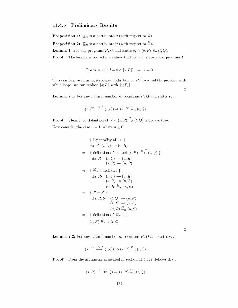
11.4.5 Preliminary Results
Proposition 1: Ovn is a partial order (with respect toO=).
Proposition 2: Dvn is a partial order (with respect toD=).
Lemma 1: For any programs P , Q and states s, t: (s, P ) Dv0 (t, Q).
Proof: The lemma is proved if we show that for any state s and program P :
∃←−−vars,−−→vars · (l = 0 ∧ [[s;P ]]) = l = 0
This can be proved using structural induction on P . To avoid the problem withwhile loops, we can replace [[s;P ]] with [[s;P1]].
2
Lemma 2.1: For any natural number n, programs P , Q and states s, t:
(s, P )0−→∗
(t, Q)⇒ (s, P )O=n (t, Q)
Proof: Clearly, by definition of Ov0, (s, P )O=0 (t, Q) is always true.
Now consider the case n+ 1, where n ≥ 0.
{ By totality of →→ }∃u,R · (t, Q)→→ (u,R)
⇒ { definition of →→ and (s, P )0−→∗
(t, Q) }∃u,R· (t, Q)→→ (u,R)
(s, P )→→ (u,R)
⇒ { O=n is reflexive }∃u,R· (t, Q)→→ (u,R)
(s, P )→→ (u,R)
(u,R)O=n (u,R)
⇒ { R = S }∃u,R, S· (t, Q)→→ (u,R)
(s, P )→→ (u, S)
(u,R)O=n (u, S)
⇒ { definition of Ovn+1 }(s, P )
O=n+1 (t, Q)
2
Lemma 2.2: For any natural number n, programs P , Q and states s, t:
(s, P )0−→∗
(t, Q)⇒ (s, P )D=n (t, Q)
Proof: From the arguments presented in section 11.3.1, it follows that:
(s, P )0−→ (t, Q)⇒ (s, P )
D=n (t, Q)
139

By definition of transitive reflexive closure, we know that:
(s, P )0−→∗
(t, Q)⇒ ∃m : � ·m ≥ 0 ∧ (s, P )0−→
m
(t, Q)
To prove the statement, we use induction on m and the fact thatD=n is reflexive
and transitive.
For the base case, when m = 0, we get that (s, P ) = (t, Q), and hence (s, P )D=n
(t, Q).
Let us assume that the result holds for a particular value of m. Now considerthe case of m+ 1:
(s, P )0−→
m+1(t, Q)
⇒ ∃u,R · (s, P )0−→ (u,R) ∧ (u,R)
0−→m
(t, Q)
⇒ { by the inductive hypothesis }∃u,R · (s, P )
0−→ (u,R) ∧ (u,R)D=n (t, Q)
⇒ { previous arguments in section 11.3.1 }∃u,R · (s, P )
D=n (u,R) ∧ (u,R)
D=n (t, Q)
⇒ { transitivity ofD=n }
(s, P )D=n (t, Q)
2
Lemma 3.1: For any natural number n, programs P , Q and state s:
(s, P )1−→ (s,Q)⇒ (s, P )
O=n (s,#1;Q)
Proof: The proof is similar to that of lemma 2.1. We consider two alternativesituations, n = 0 and n > 0. The result is trivially true in the first case. Wenow consider the case n+ 1, where n ≥ 0.
{ definition of →→ }(s,#1;Q)→→ (s,Q)
⇒ { premise and definition of →→ }(s, P )→→ (s,Q) ∧ (s,#1;Q)→→ (s,Q)
⇒ { reflexivity ofO=n }
(s, P )→→ (s,Q) ∧ (s,#1;Q)→→ (s,Q)
(s,Q)O=n (s,Q)
⇒ { u = s, R = Q and S = Q }∃u,R, S· (s, P )→→ (u,R)
(s,#1;Q)→→ (u, S)
(u,R)O=n (u, S)
⇒ { definition ofO=n+1 }
(s, P )O=n+1 (s,#1;Q)
2
140

Lemma 3.2: For any natural number n, programs P , Q and state s:
(s, P )1−→ (s,Q)⇒ (s, P )
D=n (s,#1;Q)
Proof: The proof follows directly from the argument given in section 11.3.3
and the definition ofD=n.
2
Lemma 4: For any natural number n, programs P , Q and states s, t:
(s, P ) Dvn (s,Q) ⇐⇒ (s,#1;P ) Dvn+1 (s,#1;Q)
Proof: The proof is based on the definition of the denotational semantics anda number of laws of duration calculus:
(s, P ) Dvn (s,Q)
⇐⇒ { by definition of Dvn }∃←−−vars,−−→vars · (l = n ∧ [[s;Q]])⇒ ∃←−−vars,−−→vars · [[s;P ]]
⇐⇒ { monotonicity of o
9}
∃←−−vars,−−→vars· (l = 1 ∧ Const(vars)) o
9
(l = n ∧ [[s;Q]])⇒ ∃←−−vars,−−→vars· (l = 1 ∧ Const(vars)) o
9[[s;P ]]
⇐⇒ { duration calculus and denotational semantics }∃←−−vars,−−→vars· (de ∧ −−→vars = s(vars)) o
9
(l = 1 ∧ Const(vars)) o
9
(l = n ∧ [[Q]])⇒ ∃←−−vars,−−→vars· (de ∧ −−→vars = s(vars)) o
9
(l = 1 ∧ Const(vars)) o
9[[P ]]
⇐⇒ { denotational semantics }∃←−−vars,−−→vars · ([[s; #1;Q]] ∧ l = n+ 1)⇒ ∃←−−vars,−−→vars · [[s; #1;P ]]
⇐⇒ { by definition of Dvn+1 }(s,#1;P ) Dvn+1 (s,#1;Q)
2
Lemma 5: If (s, P ) Dvn (t, Q) and n > 0 then:
∃u, P ′, Q′ · (s, P )→→ (u, P ′)
(t, Q)→→ (u,Q′)
Proof: Since →→ is total, we know that for some P ′, Q′, u and v:
(s, P )→→ (u, P ′)
(t, Q)→→ (v,Q′)
But we can decompose→→ into a number of0−→ transitions and a
1−→ transition:
141

(s, P )0−→∗
(u, P ′′)1−→ (u, P ′)
(t, Q)0−→∗
(v,Q′′)1−→ (v,Q′)
By lemmata 3.2 and 2.2, we can thus conclude that:
(u, P ′′)D=n (u,#1;P ′)
(v,Q′′)D=n (v,#1;Q′)
(u, P ′′)D=n (s, P )
(v,Q′′)D=n (t, Q)
Hence, by transitivity ofD=n:
(s, P )D=n (u,#1;P ′)
(t, Q)D=n (v,#1;Q′)
But, from the lemma premise we know that (s, P ) Dvn (t, Q) and thus:
(u,#1;P ′) Dvn (v,#1;Q′)
Now, if u 6= v, the only way in which the above refinement can be satisfied is if:
l = n ∧ [[#1;Q′]] = false
But it is easy to see that for any program P , (l = n∧ [[P ]]) is never false. Henceu = v.
2
11.4.6 Unifying the Operational and Denotational Seman-
tics
Theorem 1: For any natural number n, programs P , Q and states s, t:
(s, P ) Ovn (t, Q) ⇐⇒ (s, P ) Dvn (t, Q)
In other words, Ovn= Dvn
Proof: We prove this theorem using induction on n.
Base case: n = 0. Lemma 1 already guarantees this.
Inductive hypothesis: Let us assume that the theorem holds for n:
(s, P ) Ovn (t, Q) ⇐⇒ (s, P ) Dvn (t, Q).
Inductive case: We would now like to show that:
(s, P ) Ovn+1 (t, Q) ⇐⇒ (s, P ) Dvn+1 (t, Q).
We now consider the two directions of the proof separately:
142

• Case 1: Ovn+1⊆ Dvn+1. In this part we will be proving that the denota-tional semantics are complete with respect to the operational semantics.Equivalently, it can be seen to show that the operational semantics aresound with respect to the denotational semantics.
(s, P ) Ovn+1 (t, Q)
⇒ { definition of Ovn+1 }∃u, P ′′, Q′′· (s, P )→→ (u, P ′′)
(t, Q)→→ (u,Q′′)(u, P ′′) Ovn (u,Q′′)
⇒ { inductive hypothesis }∃u, P ′′, Q′′· (s, P )→→ (u, P ′′)
(t, Q)→→ (u,Q′′)(u, P ′′) Dvn (u,Q′′)
⇒ { definition of →→ }∃u, P ′, P ′′, Q′, Q′′· (s, P )
0−→∗
(u, P ′)
(u, P ′)1−→ (u, P ′′)
(t, Q)0−→∗
(u,Q′)
(u,Q′)1−→ (u,Q′′)
(u, P ′′) Dvn (u,Q′′)
⇒ { Lemma 4 }∃u, P ′, P ′′, Q′, Q′′· (s, P )
0−→∗
(u, P ′)
(u, P ′)1−→ (u, P ′′)
(t, Q)0−→∗
(u,Q′)
(u,Q′)1−→ (u,Q′′)
(u,#1;P ′′) Dvn+1 (u,#1;Q′′)
⇒ { Lemma 3.2 }∃u, P ′, Q′· (s, P )
0−→∗
(u, P ′)
(t, Q)0−→∗
(u,Q′)(u, P ′) Dvn+1 (u,Q′)
⇒ { Lemma 2.2 }(s, P ) Dvn+1 (t, Q)
• Case 2: Ovn⊇ Dvn. The is the dual of the first case, where we showthat the denotational semantics are sound with respect to the operationalsemantics (or, equivalently, that the operational semantics are completewith respect to the denotational semantics).
(s, P ) Dvn+1 (t, Q)
⇒ { Lemma 5 }∃u, P ′′, Q′′· (s, P )→→ (u, P ′′)
(t, Q)→→ (u,Q′′)(s, P ) Dvn+1 (t, Q)
⇒ { definition of →→ and1−→ keeps state constant }
143

∃u, P ′, P ′′, Q′, Q′′· (s, P )0−→∗
(u, P ′)
(u, P ′)1−→ (u, P ′′)
(t, Q)0−→∗
(u,Q′)
(u,Q′)1−→ (u,Q′′)
(s, P ) Dvn+1 (t, Q)
⇒ { Lemma 2.2 }∃u, P ′, P ′′, Q′, Q′′· (s, P )→→ (u, P ′′)
(t, Q)→→ (u,Q′′)
(u, P ′)1−→ (u, P ′′)
(u,Q′)1−→ (u,Q′′)
(u, P ′) Dvn+1 (u,Q′)
⇒ { Lemma 3.2 twice }∃u, P ′, P ′′, Q′, Q′′· (s, P )→→ (u, P ′′)
(t, Q)→→ (u,Q′′)
(u, P ′)D=n+1 (u,#1;P ′′)
(u,Q′)D=n+1 (u,#1;Q′′)
(u, P ′) Dvn+1 (u,Q′)
⇒ { transitivity of Dvn }∃u, P ′′, Q′′· (s, P )→→ (u, P ′′)
(t, Q)→→ (u,Q′′)(u,#1;P ′′) Dvn+1 (u,#1;Q′′)
⇒ { Lemma 4 and information from previous lines }∃u, P ′′, Q′′· (s, P )→→ (u, P ′′)
(t, Q)→→ (u,Q′′)(u, P ′′) Dvn (u,Q′′)
⇒ { inductive hypothesis and definition of →→ }∃u, P ′′, Q′′· (s, P )→→ (u, P ′′)
(t, Q)→→ (u,Q′′)(u, P ′′) Ovn (u,Q′′)
⇒ { definition of Ovn+1 }(s, P ) Ovn+1 (t, Q)
This completes the inductive case, and hence the proof.2
Corollary 1: PD= Q ⇐⇒ P
O= Q.
Proof: This follows almost immediately from Theorem 1.
{ Theorem 1 }∀n : � · Dvn= Ovn
⇒ { definition of Dv and Ov }Dv= Ov
⇒ { definition ofD= and
O= }
D==
O=
2
144

11.5 Conclusions
This chapter has unified two strictly different views of the semantics of Verilog.On one hand we have the denotational semantics which allow us to comparemathematical specifications with a Verilog program. On the other hand wehave an operational semantics which describes exactly the way in which thelanguage is interpreted. Essentially, the result is a set of laws which decide thetransformation of a Verilog program into a sequential one. This complementsthe results given in the previous chapter, where the transformations parallelisedthe code as much as possible. The two approaches complement each other andserve to expose better the dual nature of languages which combine sequentialwith parallel execution.
145

Part V
146

Chapter 12
Conclusions and Future
Work
12.1 An Overview
The main goal of this thesis is to show how standard industrial HDLs can be usedwithin a formal framework. Different research may have different motivationsfor the formalisation of a language semantics. One such motivation can be toformally document the behaviour of programs written in the language. Anothermotive may be that of providing a sound mathematical basis to serve as a toolfor program development and verification. Our choice of the subset of Verilogwe choose to formalise indicates that our primary aim is more the second thanthe first. We aimed at identifying a subset of Verilog with a clear semantics soas to enable us to produce more elegant proofs. In particular, hardware actsupon input varying over time to produce a time dependent output. It is thusdesirable to be able to talk about time related properties of such systems.
Algebraic reasoning in arithmetic and analysis has been used effectively by engi-neers for centuries and we believe that this is also the way forward in hardwareengineering. However, one would desire a mathematical interpretation of thelanguage by which to judge these laws. This is the main motivation behind thedenotational semantics (chapter 5) and the algebraic laws (chapter 6).
In particular, if a decision procedure can be used to apply these laws effectivelytowards a particular objective, their use becomes much more attractive. Onesuch application is the compilation procedure presented in chapter 10. Anotheris the interpretation of the language by a simulator. Although such an inter-pretation is usually seen as an operational semantics, there is no reason why weshould not view the operational transitions as algebraic laws in their own rightas shown in chapter 11.
12.2 Shortcomings
The evaluation of this thesis would be incomplete if it lacks to mention itsshortcomings. This section attempts to express and discuss the main ones.
Formalised subset of Verilog: The subset of Verilog which has been for-malised is rather large. However, the side condition that the programsmust not perform any concurrent reading and writing on global variables
147

is rather strong. Certain frequently used programs such as (@clk v=d
or clk) are not allowed. The main problem is that the condition is notsyntactically checkable. Conventions could have been defined to (syntac-tically) make sure that this condition is always satisfied, for example byensuring that reading is always performed at the rising edge of a globalclock, while writing is always performed at the falling edge. Alternatively,the non-deterministic semantics given in section 5.5.4 could be used toget around the problem. These non-deterministic semantics should beanalysed more thoroughly in the future.
Unknown and high impedance values: These values (denoted by x and z
respectively) are frequently used by hardware engineers to model tri-statedevices. Our basic Verilog semantics fail to handle these values and al-though section 5.5.3 discusses possible ways to handle such values anddevices, they have not been explored any further in the thesis.
Case studies: The case studies analyed in chapters 7 to 9 are rather small.Larger case studies (such as the correctness of a small processor) need tobe performed to judge better the utility of the semantics presented in thisthesis.
Mechanical proof checking: A number of rather complex theorems have beenproved in this thesis which would have benefitted from a run through amechanical proof checker. This is discussed in more detail in section 12.3.2.
The results presented thus still need considerable refinement before they canfind their place on the hardware engineer’s workbench. However, we believethat this thesis is a step towards the use of formal tools and techniques inhardware design.
12.3 Future Work
12.3.1 Other Uses of Relational Duration Calculus
Relational Duration Calculus has been developed with the semantics of Verilogin mind. However, the formulation of the calculus is much more general thanthis and should be found useful in describing other phenomena.
One of the differences between Verilog and VHDL is the concept of delta delaysin VHDL, where signal assignments are postponed until the simulator has toexecute a wait instruction1. On the other hand, variable assignments take placeimmediately.
Consider the following VHDL portion of code:
s<=0; wait for 0ns; s<=1; v=1; w=s and v
where s is a signal and v, w are variables. We would expect w to be assignedthe value 0 (0 and 1). Note that v is updated immediately, while s is not.
This two-level hierarchy can be captured in Relational Duration Calculus thanksto the typing of the relational chop operator:
1In a certain sense, this is quite similar to Verilog non-blocking assignments.
148

( −→s = 0∧de∧Const({v, w})
){s,v,w}
o
9
(( −→s = 1∧de∧Const({v, w})
){v,w}
o
9
( −→v = 1∧de∧Const({w})
){v,w}
o
9
( −→w =←−v ∧←−s∧de∧Const({v})
))
In fact, this technique should also be applicable to other languages with aninherently built synchronisation mechanism such as BSP. Going one step further,one can construct a language with multiple ‘synchronisation layers’. VHDL hasonly two such layers, the local (variables) and delta level (signals), as does BSP.But one may construct a language with a whole family of such layers to aidprogramming in, say, a network of distributed systems. The semantics of sucha language should be elegantly expressible in Relational Duration Calculus.
12.3.2 Mechanised Proofs
The work presented in this thesis can be pushed forward along various paths.One obvious missing aspect is machine verified proofs of the theorems presented.Ideally, one should provide support for machine proofs in Relational DurationCalculus.
Not much work has yet been done in mechanising Duration Calculus proofs.[SS93] embedded Duration Calculus in PVS and proved a number of numberof properties of standard case studies. They have also defined a number oftactics, for instance, to automatically prove statements in a decidable subset ofDuration Calculus.
[Pac94] investigated the use of JAPE [SB93], a visual proof calculator, to prove anumber of hardware implementations of standard case studies correct. However,the proofs were given with respect to a number of Duration Calculus laws, asopposed to the underlying definitions or axioms. A number of tactics usefulin transforming some real-time specifications into a format closer to hardwarehave also been presented there.
Embedding Relational Duration Calculus and the given Verilog semantics intoa standard theorem prover and proving the correctness of the algebraic lawswould allow the verification of the proofs given in the thesis. The hardwarecompilation and simulation semantics could then be encoded as proof tactics.
12.3.3 Real-Time Properties and HDLs
An area which is only briefly touched upon in this thesis is the verification ofreal-time properties of programs written in a hardware description language.The use of Duration Calculus to specify the semantics of Verilog allows us tohandle such proofs in a straightforward manner. Unfortunately, we are not awareof much other work done for this particular style of specification in conjunctionwith HDLs. It would be interesting to study this area in more detail and seewhat useful results can be achieved.
12.3.4 Extending the Sub-Languages
Another aspect which should ideally be extended is the sub-language which iscompiled into hardware-like format. Other constructs (such as fork ...join)
149

and instructions (such as @v) can be converted into a hardware-like format with-out too much difficulty. One would still, however, desire a proof of correctnessfor these additional transformations.
The same can be said of the comparison between the operational and denota-tional semantics.
12.4 Conclusion
The main aim of this thesis was to study the development of a formal frameworkfor Verilog, as a typical industrial-strength hardware description language. Themain achievement was the building of a basis for such a framework, but morework still needs to be done in order to make this framework robust and generalenough to be useful in a real-life hardware development environment.
150

Bibliography
[Bal93] Felice Balarin. Verilog HDL modelling styles for formal verifica-tion. In D. Agnew and L. Claesen, editors, Computer HardwareDescription Languages and their Applications (A-32), pages 453–466. Elsevier Science Publishers BV (North-Holland), 1993.
[BB92] J.C.M Baeten and J.A. Bergstra. Discrete time process algebra.In W.R. Cleaveland, editor, Proceedings of CONCUR ’92, number630 in Lecture Notes in Computer Science, pages 401–420. Springer,1992.
[BB93] J.C.M Baeten and J.A. Bergstra. Real time process algebra withinfinitesimals. Technical Report P9325, Programming ResearchGroup, University of Amsterdam, October 1993.
[BFK95] Peter T. Breuer, Luis Sanchez Fernandez, and Carlos DelgadoKloos. A simple denotational semantics, proof theory and a val-idation condition generator for unit-delay VHDL. Formal Methodsin System Design, 7:27–51, 1995.
[BG96] C. Bolchini and C. Ghezzi. Software systems: Languages, modelsand processes. In Giovanni de Micheli and Mariagiovanna Sami,editors, Software Hardware Co-design, volume 310 of NATO ASIseries (Series E — Applied Sciences), pages 397–426. Kluwer Aca-demic publishers (Netherlands), 1996.
[BGM95] E. Borger, U. Glasser, and W. Muller. Formal definition of anabstract VHDL ’93 simulator by EA-machines. In C. Delgado Kloosand P.T. Breuer, editors, Formal Semantics for VHDL, pages 107–139. Kluwer Academic Press Boston/London/Dordrecht, 1995.
[Bla96] Gerald M. Blair. Verilog — accellerating digital design. IEE Elec-tronics and Communication Engineering Journal, 9(2):68–72, 1996.
[Boc82] Gregor V. Bochmann. Hardware specification with temporal logic:An example. IEEE Transactions on Computers, C-31(3):223–231,March 1982.
[Bor95] Editor Dominique Borrione. Formal methods in system design, spe-cial issue on VHDL semantics. Volume 7, Nos. 1/2, Aug 1995.
[Bou97] Richard J. Boulton. A tool to support formal reasoning about com-puter languages. In E. Brinksma, editor, Proceedings of the ThirdInternational Workshop on Tools and Algorithms for the Construc-tion and Analysis of Systems (TACAS ’97), Enschede, The Nether-lands, number 1217 in Lecture Notes in Computer Science, pages81–95. Springer, April 1997.
151

[Bry86] Randal E. Bryant. Can a simulator verify a circuit? In G. Milneand P.A. Subrahmanyam, editors, Formal Aspects of VLSI Design,pages 125–136. Elsevier Science Publisher B.V., 1986.
[BS95] Dominique Borrione and Ashraf Salem. Denotational semantics ofa synchronous VHDL subset. Formal Methods in System Design,7:53–71, 1995.
[BSC+94] C. Bayol, B. Soulas, F. Corno, P. Prinetto, and D. Borrione. A pro-cess algebra interpretation of a verification oriented overlanguageof VHDL. In EURO-DAC 1994/EURO-VHDL ’94, pages 506–511.IEEE CS Press, 1994.
[BSK93] P.T. Breuer, L. Sanchez, and C. Delgado Kloos. Clean formal se-mantics for VHDL. In European Design and Test Conference, Paris,pages 641–647. IEEE Computer Society Press, 1993.
[Cam90] Albert Camilleri. Simulating hardware specifications within a theo-rem proving environment. International Journal of Computer AidedVLSI design, (2):315–337, 1990.
[CGH+93] Massimiliano Chiodo, Paolo Giusto, Harry Hsieh, Attila Jurecska,Luciano Lavagno, and Alberto Sangiovanni-Vincentelli. A formalspecification model for hardware/software codesign. In Proceedingsof International Workshop on Software-Hardware Codesign, Octo-ber 1993.
[CGM86] Albert Camilleri, Mike Gordon, and Tom Melham. Hardware ver-ification using higher order logic. Technical Report 91, Universityof Cambridge Computing Laboratory, 1986.
[CHF96] Ching-Tsun Chou, Jiun-Lang Huang, and Masahiro Fujita. A high-level language for programming complex temporal behaviours andits translation into synchronous circuits. September 1996.
[CP88] Paolo Camurati and Paola Prinetto. Formal verification of hardwarecorrectness: Introduction and survey of current research. IEEEComputer, pages 8–19, July 1988.
[Dav93] K.C. Davis. A denotational definition of the VHDL simulation ker-nel. In P. Agnew, L. Claesen, and R. Camposano, editors, Pro-ceedings of the 11th IFIP WG 10.2 International Conference onComputer Hardware Description Languages and their applicationsCHDL ’93, pages 523–536, 1993.
[Des96a] Chrysalis Symbolic Design. Design for verification strategies op-timize advanced verification techniques, December 1996. availablefrom http://chrys.chrysalis.com/techinfo/.
[Des96b] Chrysalis Symbolic Design. Symbolic logic technology, January1996. available from http://chrys.chrysalis.com/techinfo/.
[Des96c] Chrysalis Symbolic Design. What is formal verification, January1996. available from http://chrys.chrysalis.com/techinfo/.
[DHP95] Gert Dohmen, Ronald Herrmann, and Hergen Pargmann. Trans-lating VHDL into functional symbolic finite-state models. FormalMethods in System Design, 7:125–148, 1995.
152

[Fou91] Micheal P. Fourman. Proof and design — machine-assisted formalproof as a basis for behavioural design tools. Technical ReportLFCS-91-319, Laboratory for the foundations of Computer Science,The University of Edinburgh, 1991.
[Fra95] Martin Franzle. On appropiateness of the digitality abstrac-tion taken in duration calculus to implementation developement.ProCoS document, Christian-Albrechts-Universitat Kiel, Germany,1995.
[GG95] D.J. Greaves and M.J.C. Gordon. Checking equivalencebetween synthesised logic and non-synthesisable behaviouralprototypes. Research Proposal, 1995. available fromhttp://www.cl.cam.ac.uk/users/djs1002/verilog.project.
[GG98] M.J.C. Gordon and A. Ghosh. Language independent RTL seman-tics. In Proceedings of IEEE CS Annual Workshop on VLSI: SystemLevel Design, Florida, USA, 1998.
[Gol92] Robert Goldblatt. Logics of Time and Computation, chapter 6:Temporal Logic. Number 7 in CLSI lecture notes. Center for theStudy of Language and Information, second edition, 1992.
[Gol94] Steve Golson. State machine design techniques for Verilog andVHDL. Synopsys Journal of High-Level Design, September 1994.Available from www.synopsys.com).
[Gol96] Ulrich Golze. VLSI Chip Design with the Hardware DescriptionLanguage VERILOG: an introduction based on a large RISC pro-cessor. Springer, 1996.
[Goo93a] K.G.W. Goossens. The formalisation of a hardware description lan-guage in a proof system: Motivation and applications. In Proceed-ings of the XIII Conference of the Brazilian Computer Society, Flo-rianopolis, Brazil, September 1993.
[Goo93b] K.G.W. Goossens. Structure and behaviour in hardware verifica-tion. In Jeffrey J. Joyce and Carl-Johan H. Seger, editors, HigherOrder Logic Theorem Proving and its applications, 6th InternationalWorkshop, HUG ’93, Vancouver, B.C. Canada, number 780 in Lec-ture Notes in Computer Science, pages 73–87, 1993.
[Goo95] K.G.W. Goossens. Reasoning about VHDL using operational andobservational semantics. Technical Report SI/RR-95/06, Diparti-mento di Scienze dell’ Informazione, Universita degli Studi di Roma,‘La Sapienza’, via Salaria, 113-I-00198, Roma, April 1995.
[Gor95] Mike Gordon. The semantic challenge of Verilog HDL. In Pro-ceedings of the tenth annual IEEE symposium on Logic in Com-puter Science (LICS ’95) San Diego, California, pages 136–145,June 1995.
[Gor98] M.J.C. Gordon. Event and cycle semantics of hardwaredescription languages v1.4, January 1998. available fromhttp://www.cl.cam.ac.uk/users/djs1002/verilog.project/.
[H+85] C.A.R. Hoare et al. Laws of programming — a tutorial paper.Technical Monograph PRG-45, Oxford University Computing Lab-oratory, 1985.
153

[Hay82] John P. Hayes. A unified switching theory with applications to VLSIdesign. Proceedings of the IEEE, 70(10):1140–1151, 1982.
[HB92] Jifeng He and Jonathan Bowen. Time interval semantics and imple-mentation of a real-time programming language. In Proceedings ofthe 4th Euromicro Workshop in Computing, pages 173–192, August1992.
[HB93] Jifeng He and S.M. Brien. Z description of duration calculus.Technical report, Oxford University Computing Laboratory (PRG),1993.
[He93] Jifeng He. Synchronous realization of circuits. ProCos documentOU HJF 17/1, Oxford University Computing Laboratory, Program-ming Research Group, Wolfson Building, Parks Road, Oxford, Oc-tober 1993.
[He94] Jifeng He. From CSP to hybrid systems. In A.W. Roscoe, editor,A Classical Mind, chapter 11, pages 171–189. Prentice-Hall, 1994.
[Hea93] Thomas Heath. Automating the compilation of software into hard-ware. Master’s thesis, Oxford University Computing Laboratory,Oxford University, 1993.
[Her88] John Herbert. Formal verification of basic memory devices. Tech-nical Report 124, University of Cambridge Computing Laboratory,1988.
[HH94] C.A.R. Hoare and Jifeng He. Specification and implementation ofa flashlight. ProCoS report, Oxford University Computing Labora-tory, 1994.
[HHF+94] Jifeng He, C.A.R. Hoare, Martin Franzle, Markus Muller-Olm,Ernst-Rudiger Olderog, Michael Schenke, Michael R. Hansen, An-ders P. Ravn, and Hans Rischel. Provably correct systems. Technicalreport, ProCoS, 1994.
[HHS93a] C.A.R. Hoare, Jifeng He, and A. Sampaio. From algebra to op-erational semantics. Information Processing Letters, 45(2):75–80,February 1993.
[HHS93b] C.A.R. Hoare, Jifeng He, and Augusto Sampaio. Normal form ap-proach to compiler design. ACTA Informatica, 30:701–739, 1993.
[HI96] Dang Van Hung and Ko Kwang Il. Verification via digitized mod-els of real-time systems. Research UNU/IIST Report No. 54,The United Nations University, International Institute for SoftwareTechnology, P.O. Box 3058, Macau, February 1996.
[HJ94] Jifeng He and Zheng Jianping. Simulation approach to provablycorrect hardware compilation. In Formal Techniques in Real-Timeand Fault Tolerant Systems, number 863 in Lecture Notes in Com-puter Science, pages 336–350. Springer-Verlag, 1994.
[HJ98] C.A.R. Hoare and He Jifeng. Unifying Theories of Programming.Prentice-Hall Series in Computer Science, 1998.
154

[HMC96] Jifeng He, Quentin Miller, and Lei Chen. Algebraic laws for BSPprogramming. In Proceedings of EUROPAR 1996, number 1124in Lecture Notes in Computer Science, pages 359–368. Springer-Verlag, 1996.
[HMM83] Joseph Halpern, Zohar Manna, and Ben Moszkowski. A hardwaresemantics based on temporal intervals. In 10th International Col-loqium on Automata, Languages and Programming, number 154in Lecture Notes in Computer Science, pages 278–291. Springer-Verlag, 1983.
[HO94] Jifeng He and Ernst-Rudiger Olderog. From real-time specificationto clocked circuit. ProCoS document, Department of ComputerScience, Technical University of Denmark, DK-2800, Lyngby, Den-mark, 1994.
[Hoa85] C.A.R. Hoare. Communicating Sequential Processes. Prentice-HallInternational, 1985.
[Hoa90] C.A.R. Hoare. A theory for the derivation of C-MOS circuit designs.In Beauty is our Business, Texts and monographs in ComputerScience. Springer-Verlag, 1990.
[Hoa94] C.A.R. Hoare. Mathematical models for computer science. LectureNotes for Marktoberdorf Summer School, August 1994.
[Hol97] Clive Holmes. VHDL language course. Technical report, RutherfordAppleton Laboratory, Microelectronics Support Centre, Chilton,Didcot, Oxfordshire, February 1997.
[HP94] C.A.R. Hoare and Ian Page. Hardware and software: The closinggap. Transputer Communications, 2(2):69–90, June 1994.
[HRS94] K.M. Hansen, A.P. Ravn, and V. Stravridou. From safety analysisto formal specification. ProCoS document DTH KMH 1/1, De-partment of Computer Science, Technical University of Denmark,DK-2800, Lyngby, Denmark, February 1994.
[HZ94] M.R. Hansen and Chaochen Zhou. Duration calculus: Logical foun-dations. Formal Aspects of Computing, 6(6A):826–845, 1994.
[HZS92] Michael Hansen, Chaochen Zhou, and Jørgen Straunstrup. A real-time duration semantics for circuits. In Proceedings of Tau ’92:1992 Workshop on Timing Issues in the Specification and Synthesisof Digital Systems, ACM/SIDGA, September 1992.
[IEE95] IEEE. Draft Standard Verilog HDL (IEEE 1364). 1995.
[Joy89] Jeffrey J. Joyce. A verified compiler for a verified microprocessor.Technical Report 167, University of Cambridge Computer Labora-tory, March 1989.
[JS90] Geraint Jones and M. Sheeran. Circuit design in RUBY. In JørgenStraunstrap, editor, Formal Methods for VLSI Design, pages 13–70.Elsevier Science Publications BV, 1990.
[JU90] Mark B. Josephs and Jan Tijmen Udding. An algebra for delay-insensitive circuits. Technical Report WUCS-89-54, Department ofComputer Science, Washington University, Campus Box 1045, OneBrookings Drive, Saint Louis, MO 63130-4899, March 1990.
155

[KAJW93] Sunjaya Kumar, James H. Aylor, Barry W. Johnson, and W.A.Wulf. A framework for software-hardware co-design. IEEE Com-puter, 26(12):39–46, December 1993.
[KB95] Carlo Delgado Kloos and Peter T. Breuer. Formal Semantics forVHDL. Number 307 in The Kluwer International Series in Engi-neering and Computer Science. Kluwer Academic Publishers, 1995.
[KLMM95] D. Knapp, T. Ly, D. MacMillen, and R. Miller. Behavioral syn-thesis methodology for HDL-based specification and validation. InProceedings of DAC ’95, 1995.
[Kroon] Thomas Kropf. Benchmark-circuits for hardware-verification v1.2.1.Technical Report SFB 358-C2-4/94, Universitat Karlsruhe, 1996(updated version).
[KW88] K. Keutzer and W. Wolf. Anatomy of a hardware compiler. InDavid S. Wise, editor, Proceedings of the SIGPLAN ’88 Conferenceon Programming Lanugage Design and Implementation (SIGPLAN’88), pages 95–104. ACM Press, June 1988.
[Lam85] Leslie Lamport. On interprocess communication. Technical Re-port 8, Systems Research Center (SRC), December 1985.
[Lam91] Leslie Lamport. The temporal logic of actions (TLA). Technical Re-port 79, Digital Equipment Corporation Systems Research centre,1991.
[Lam93] L. Lamport. Hybrid systems in TLA+. In R. L. Grossman,A. Nerode, A. P. Ravn, and H. Rischel, editors, Hybrid Systems,volume 736 of Lecture Notes in Computer Science, pages 77–102.Springer-Verlag, 1993.
[LL95] Yanbing Li and Miriam Leeser. HML: An innovative hardware de-scription language and its translation to VHDL. Technical ReportEE-CE9-95-2, School of Electrical Engineering, Cornell University,Ithaca, 1995.
[LMS86] Roger Lipsett, Erich Marchner, and Moe Shahdad. VHDL — thelanguage. IEEE Design and Test, 3(2):28–41, April 1986.
[LS93] Leslie Lamport and Merz Stephan. Hybrid systems in TLA+. InR.L. Grossman, A. Nerode, A.P. Ravn, and H. Rischel, editors,Hybrid Systems, number 736 in Lecture Notes in Computer Science,pages 77–102. Springer-Verlag, 1993.
[LS94] Leslie Lamport and Merz Stephan. Specifying and verifying faulttolerant systems. In Formal Techniques in Real-Time and Fault Tol-erant Systems, number 863 in Lecture Notes in Computer Science,pages 41–76. Springer-Verlag, 1994.
[Man81] Zohar Manna. Verification of sequential programs using temporalaxiomatization. Technical Report STAN-CS-81-877, Department ofComputer Science, Stanford University, September 1981.
[May90] D. May. Compiling occam into silicon. In C. A. R. Hoare, editor,Developments in Concurrency and Communication, University ofTexas at Austin Year of Programming Series, chapter 3, pages 87–106. Addison-Wesley Publishing Company, 1990.
156

[Maz71] Antoni W. Mazwikiewicz. Proving algorithms by tail functions.Information and Control, 18:220–226, 1971.
[Mel87] Thomas Melham. Abstraction mechanisms for hardware verifica-tion. Technical Report 106, University of Cambridge ComputerLaboratory, 1987.
[Mil83] G.J. Milne. Circal: A calculus for circuit description. IntegrationVLSI Journal, 1(2,3), 1983.
[Mil85a] G.J. Milne. Circal and the representation of communication, con-currency and time. ACM Transactions on Programming Languagesand Systems, 7(2):270–298, 1985.
[Mil85b] G.J. Milne. Simulation and verification: Related techniques forhardware analysis. In C.J. Koomen and T. Moto-oka, editors, Pro-ceedings of the 7th International Conference on Computer HardwareDesign Language Applications (CHDL ’85), Tokyo, pages 404–417,1985.
[Mil89] R. Milner. Communication and Concurrency. Prentice Hall Inter-national, 1989.
[Mil91] G.J. Milne. Formal description and verification of hardware timing.IEEE transactions on Computers, 40(7):811–826, July 1991.
[Mil94] G.J. Milne. Formal Specification and Verification of Digital Sys-tems. McGraw-Hill, 1994.
[MM83] Ben Moszkowski and Zohar Manna. Reasoning in interval temporallogic. Technical Report STAN-CS-83-969, Department of ComputerScience, Stanford University, July 1983.
[Mol89] F. Moller. The semantics of CIRCAL. Technical Report HDF-3-89, Department of Computer Science, University of Strathclyde,Glasgow, Scotland, 1989.
[Moo94] J. Strother Moore. A formal model of asynchronous communica-tion and its use in mechanically verifying a biphase mark protocol.Formal Aspects of Computation, 6:60–91, 1994.
[Mos84] Ben Moszkowski. Executing temporal logic programs. TechnicalReport 55, University of Cambridge Computer Laboratory, 1984.
[Mos85] Ben Moszkowski. A temporal logic for multilevel reasoning abouthardware. Computer, 2(18):10–19, February 1985.
[Mos86] Ben Moszkowski. Executing Temporal Logic Programs. CambridgeUniversity Press, 1986.
[MP81] Zohar Manna and Amir Pnueli. Verification of concurrent programs:the temporal framework. In Robert S. Boyer and J. Strother Moore,editors, The Correctness Problem in Computer Science, Int. LectureSeries in Computer Science, pages 215–273. Academic Press, 1981.
[MP87] Zohar Manna and Amir Pnueli. A hierarchy of temporal proper-ties. Technical Report STAN-CS-87-1186, Department of ComputerScience, Stanford University, October 1987.
157
[MP90] Zohar Manna and Amir Pnueli. A hierarchy of temporal properties.In Proceedings of the 9th Annual ACM Symposium on Principles ofDistributed Computing, pages 377–408. ACM Press, 1990.
[MP94] Zohar Manna and Amir Pnueli. Models for reactivity. In 3rd In-ternational School and Symposium on Formal Techniques in RealTime Systems and Fault Tolerant Systems, Lubeck Germany, 1994.
[MR93] Paulo C. Masiero and Anders P. Ravn. Refinement of real-timespecifications. ProCoS II document, Department of Computer Sci-ence, Technical University of Denmark, DK-2800, Lyngby, Den-mark, 1993.
[MW84] Zohar Manna and P.L. Wolper. Synthesis of computer processesfrom temporal logic specifications. ACM Transactions on Program-ming Languages and Systems, 6(1):68–93, January 1984.
[NH84] R. De Nicola and M.C.B. Hennessy. Testing equivalences for pro-cesses. Theoretical Computer Science, 34:83–133, 1984.
[Nor96] Anders Nordstrom. Formal verification — a viable alternative tosimulation? In Proceedings of International Verilog HDL Confer-ence, February 1996.
[OC95] Serafin Olcoz and Jose Manuel Colom. A colored Petri net modelof VHDL. Formal Methods in System Design, 7:101–123, 1995.
[Ope93] Open Verilog International. Verilog Hardware Description LanguageReference Manual (Version 2.0). Open Verilog, March 1993.
[Pac94] Gordon J. Pace. Duration calculus: From parallel specificationsto clocked circuits. Master’s thesis, Oxford University ComputingLaboratory, 1994.
[Pag93] Ian Page. Automatic systems synthesis: A case study.Technical report, Oxford University Computing Laboratory(PRG), 1993. Available from http://www.comlab.ox.ac.uk in/oucl/hwcomp.html.
[Pag96] Ian Page. Constructing hardware-software systems from a singledescription. Journal of VLSI Signal Processing, 12(1):87–107, 1996.
[Pag97] Ian Page. Hardware-software co-synthesis research at Oxford.UMIST Vacation School on Hardware/Software Codesign, 1997.
[Pal96] Samir Palnitkar. Verilog HDL: A Guide to Digital Design and Syn-thesis. Prentice Hall, New York, 1996.
[Per91] D.L. Perry. VHDL. McGraw-Hill, 1991.
[PH98] Gordon J. Pace and Jifeng He. Formal reasoning with Verilog HDL.In Proceedings of the Workshop on Formal Techniques in Hardwareand Hardware-like Systems, Marstrand, Sweden, June 1998.
[PL91] Ian Page and Wayne Luk. Compiling occam into field-programmable gate arrays. In Wayne Luk and Will Moore, editors,FPGAs, pages 271–283. Abingdon EE&CS books, 1991.
158

[Poo95] Rob Pooley. Integrating behavioural and simulation modelling.Technical Report ECS-CSG-8-95, Computer Systems Group, De-partment of Computer Science, University of Edinburgh, The King’sBuildings, Edinburgh, March 1995.
[PR95] P.K. Pandya and Y.S. Ramakrishna. A recursive mean-value cal-culus. Technical Report TR-95/3, Tata Institute of FundamentalResearch, Bombay, India, 1995.
[Pro97] The Verilog Formal Equivalence (VFE) Project. Synthesiz-able Verilog: Syntax and semantics, 1997. available fromhttp://www.cl.cam.ac.uk/users/djs1002/verilog.project.
[Pyg92] C.H. Pygott. Will proof replace simulation? In C.A.R. Hoareand M.J.C. Gordon, editors, Mechanized Reasoning and HardwareDesign, pages 21–33. Prentice-Hall International, 1992.
[Qiw96] Xu Qiwen. Semantics and verification of extended phase transitionsystems in duration calculus. Research UNU/IIST Report No. 72,The United Nations University, International Institute for SoftwareTechnology, P.O. Box 3058, Macau, June 1996.
[Rav95] Anders P. Ravn. Design of embedded real-time computing sys-tems. Technical Report ID-TR:1995-170, Department of ComputerScience, Technical University of Denmark, Building 344, DK-2800Lyngby, Denmark, October 1995.
[RH86] A.W. Roscoe and C.A.R. Hoare. The laws of occam programming.Technical Monograph PRG-53, Oxford University Computing Lab-oratory, 1986.
[RH88] A.W. Roscoe and C.A.R. Hoare. The laws of occam programming.Theoretical Computer Science, 60(2):177–229, September 1988.
[Ris92] Hans Rischel. A duration calculus proof of Fisher’s mutual exclusionprotocol. ProCoS document DTH HR 4/1, Department of Com-puter Science, Technical University of Denmark, DK-2800, Lyngby,Denmark, December 1992.
[RK95] Ralf Reetz and Thomas Kropf. A flowgraph semantics of VHDL:Toward a VHDL verification workbench in HOL. Formal Methodsin System Design, 7:73–99, 1995.
[Rus95] David M. Russinoff. A formalization of a subset of VHDL in theBoyer-Moore logic. Formal Methods in System Design, 7:7–25, 1995.
[Sam93] A. Sampaio. An algebraic approach to compiler design. TechnicalMonograph PRG-110, Oxford University Computing Laboratory,1993.
[SB93] Bernard Sufrin and Richard Bornat. The gist of JAPE.Technical report, Oxford University Computing Laboratory(PRG), 1993. Available from http://www.comlab.ox.ac.uk/ inoucl/bernard.sufrin/jape.shtml.
[Sch96] Michael Schenke. Transformational design of real-time systems.Acta Informatica, 1996. To appear.
159

[Sch97] Michael Schenke. Modal logic and the duration calculus. To appear,1997.
[SD97] Michael Schenke and Michael Dossis. Provably correct hard-ware compilation using timing diagrams. Available fromhttp://semantic.Informatik.Uni-Oldenburg.DE/
persons/michael.schenke/, 1997.
[SHL94] Morten Ulrik Sørensen, Odd Eric Hansen, and Hans HenrikLøvengreen. Combining temporal specification techniques. Pro-CoS document DTU MUS 1/2, Department of Computer Science,Technical University of Denmark, DK-2800, Lyngby, Denmark, May1994.
[Smi96] Douglas J. Smith. VHDL and Verilog compared and contrasted— plus modelled example written in VHDL, Verilog and C. InProceedings of the 33rd Design Automation Conference (Las VegasNV, USA), pages 771–776, 1996.
[SMSV83] R.L. Schwartz, P.M. Melliar-Smith, and F.H. Vogt. An intervalbased temporal logic. In Proceedings of the second annual ACMsymposium on Principles of Distributed Computing, Montreal, Que-bec, Canada, pages 173–186, 1983.
[Spi92] J.M. Spivey. The Z Notation: A Reference Manual (2nd edition).Prentice Hall International, 1992.
[Spi97] Michael Spivey. Deriving a hardware compiler from operationalsemantics. submitted to ACM TOPLAS, 1997.
[SS93] Jens U. Skakkebaek and N. Shankar. A duration calculus proofchecker: Using PVS as a semantic framework. Technical ReportSRI-CSL-93-10, SRI, 1993.
[SS94] Jens U. Skakkebaek and N. Shankar. Towards a duration calculusproof assistant in PVS. In H. Langmaack, W.P. Roever, and J. Vy-topil, editors, Formal Techniques in Real-Time and Fault TolerantSystems, number 863 in Lecture Notes in Computer Science, pages660–679. Springer-Verlag, 1994.
[SSMT93] E Sternheim, R. Singh, R. Madhavan, and Y. Trivedi. Digital Designand Synthesis with Verilog HDL. Automata Publishing Company,1993.
[Ste97] Daryl Stewart. Modelling Verilog port connections, 1997. Avail-able from http://www.cl.cam.ac.uk/ in/users/djs1002/verilog.project/.
[SW74] Christopher Strachey and Christopher P. Wadsworth. Continua-tions: A mathematical semantics for handling full jumps. TechnicalMonograph PRG-11, Programming Research Group, Oxford Uni-versity Computing Laboratory, 1974.
[Tan84] A.S. Tanenbaum. Structured Computer Organization (3rd edition).Prentice-Hall International, 1984.
160

[Tan88] Tong Gao Tang. A temporal logic language for hardware simulation,specification and verification. Technical Report CMU-CS-88-194,Department of Computer Science, CMU, Pittsburgh, September1988.
[Tas90] John Peter Van Tassel. The semantics of VHDL with VAL andHOL: Towards practical verification tools. Technical Report 196,University of Cambridge Computer Laboratory, June 1990.
[Tas92] John Peter Van Tassel. A formalization of the VHDL simulationcycle. Technical Report 249, University of Cambridge ComputerLaboratory, March 1992.
[TH91] John Peter Van Tassel and David Hemmendinger. Toward formalverification of VHDL specifications. In Luc Claesen, editor, AppliedFormal Methods for VLSI design, pages 399–408. Elsevier SciencePublications, 1991.
[Tho95] Donald E. Thomas. The Verilog HDL. Kluwer Academic, Boston,Massachusetts, second edition, 1995.
[Win86] Glynn Winskel. Models and logic of MOS circuits. In InternationalSummer School on Logic of Programming and Calculi of DiscreteSystems, Marktoberdorf, Germany, 1986.
[Win87] Glynn Winskel. Relating two models of hardware. In D.H. Pitt,A. Poigne, and D.E. Rydeheard, editors, Category Theory and Com-puter Science (Edinburgh, U.K., September 1987), number 283 inLecture Notes in Computer Science, pages 98–113. Springer-Verlag,1987.
[WMS91] Philip A. Wilsey, Timothy J. McBrayer, and David Sims. Towardsa formal model of VLSI systems compatible with VHDL. In A. Ha-laas and P.B. Denyer, editors, VLSI ’91, pages 225–236. ElsevierScience Publishers BV (North-Holland), Amsterdam, The Nether-lands, August 1991.
[Wol93] W.H. Wolf. Software hardware co-design. Special Issue of IEEEDesign and Test, 10(3):5, September 1993.
[XJZP94] Yu Xinyao, Wang Ji, Chaochen Zhou, and Paritosh K. Pandya. For-mal design of hybrid systems. Research UNU/IIST Report No. 19,The United Nations University, International Institute for SoftwareTechnology, P.O. Box 3058, Macau, 1994.
[Yoe90] Michael Yoeli. Formal Verification of hardware design, chapter 6:Temporal Logic, pages 159–165. The Institute of Electrical andElectronics Engineers, Inc, 1990.
[ZH92] Chaochen Zhou and C.A.R. Hoare. A model for synchronous switch-ing circuits and its theory of correctness. Formal Methods in SystemDesign, 1(1):7–28, July 1992.
[ZH96a] Chaochen Zhou and Michael R. Hansen. Chopping a point. Techni-cal report, Department of Information Technology, Technical Uni-versity of Denmark, March 1996.
161

[ZH96b] Chaochen Zhou and Michael R. Hansen. Chopping a point. InHe Jifeng, John Cooke, and Peter Wallis, editors, BCS-FACS 7thRefinement Workshop, Electronic Workshops in Computing, pages256–266. Springer-Verlag, 1996.
[ZHK96] Ping Zhou, Jozef Hooman, and Ruurd Kuipei. Compositional veri-fication of real-time systems with explicit clock temporal logic. For-mal Aspects of Computing, 8(3):294–323, 1996.
[Zho93] Chaochen Zhou. Duration calculi: An overview. In Dines Bjørner,Manfred Broy, and Igor V. Pottosin, editors, Formal Methods inProgramming and their Applications, number 735 in Lecture Notesin Computer Science, pages 256–266. Springer-Verlag, 1993.
[ZHR91] Chaochen Zhou, C.A.R. Hoare, and Anders P. Ravn. A calculus ofdurations. Information Processing Letters, 40(5):269–276, 1991.
[ZHRR91] Chaochen Zhou, Michael R. Hansen, Anders Ravn, and HansRischel. Duration specifications for shared processors. In J. Vy-topil, editor, Formal Techniques in Real Time and Fault TolerantSystems, number 571 in Lecture Notes in Computer Science, pages21–32. Springer-Verlag, 1991.
[ZHX95a] Chaochen Zhou, Dang Van Hung, and Li Xiaoshan. A durationcalculus with infinite intervals. Research UNU/IIST Report No. 40,The United Nations University, International Institute for SoftwareTechnology, P.O. Box 3058, Macau, 1995.
[ZHX95b] Chaochen Zhou, Dang Van Hung, and Li Xiaoshan. A duration cal-culus with infinite intervals. In Horst Reichel, editor, Fundamentalsof Computation, number 965 in Lecture Notes in Computer Science,pages 16–41. Springer-Verlag, 1995.
[ZRH93] Chaochen Zhou, A.P. Ravn, and M.R. Hansen. An extended dura-tion calculus for hybrid real-time systems. In Robert L. Grossman,Anil Nerode, Anders P. Ravn, and Hans Rishel, editors, HybridSystems, number 736 in Lecture Notes in Computer Science, pages36–59. Springer-Verlag, 1993.
[ZX94] Chaochen Zhou and Li Xiaoshan. A mean-value duration calculus.In A.W. Roscoe, editor, A Classical Mind. Prentice-Hall, 1994.
[ZX95] Chaochen Zhou and Li Xiaoshan. A mean-value duration calcu-lus. Research UNU/IIST Report No. 5, The United Nations Uni-versity, International Institute for Software Technology, P.O. Box3058, Macau, March 1995.
162