Handling Qualities of a Blended Wing Body Aircraft Handling Qualities of a Blended Wing Body Aircraft Timothy Shaw Peterson Master of Applied Science Institute for Aerospace Studies

Handling Qualities of a Blended Wing Body Aircraft

by

Timothy Shaw Peterson

A thesis submitted in conformity with the requirementsfor the degree of Master of Applied Science

Institute for Aerospace StudiesUniversity of Toronto

Copyright c© 2011 by Timothy Shaw Peterson

Abstract

Handling Qualities of a Blended Wing Body Aircraft

Timothy Shaw Peterson

Master of Applied Science

Institute for Aerospace Studies

University of Toronto

2011

The blended wing body (BWB) is a tailless aircraft with the potential to use 27%

less fuel than a conventional aircraft with the same passenger capacity and range. The

primary purpose of the current study was to determine the handling qualities of the

BWB, using piloted-handling trials in a moving-base simulator. The secondary purpose

was to determine the effect of simulator motion on handling-quality ratings. De Castro

conducted piloted-handling trials in a fixed-base simulator. De Castro’s tasks and flight

model were modified in the current study. In the current study, three subjects rated the

handling qualities as Level 1 or 2, depending on the task. Simulator motion did not have

a significant effect on the results.

ii

Acknowledgements

I would like to thank Professor Peter Grant for welcoming me into the Vehicle Simulation

Group and sharing his knowledge. Professor Grant gave me a choice of several interesting

thesis topics; I appreciate being able to pick the one I found most exciting. I would also

like to thank Bruce Haycock, Stacey Liu, and Amir Naseri for their help with setting

up the piloted-handling trials and their expertise in flight simulation. To the pilots who

volunteered for the handling trials — I thank you for participating. This research was

made far more meaningful because of your contribution.

I am grateful to my wife, Vanessa, for encouraging me to undertake the challenge of

graduate studies and supporting me throughout. I would like to thank my parents for

sparking my interest in aerospace and for showing me the importance of lifelong learning.

iii

Contents

1 Introduction 1

1.1 Background . . . . . . . . . . . . . . . . . . . . . . . . . . . . . . . . . . 1

1.2 Literature Review . . . . . . . . . . . . . . . . . . . . . . . . . . . . . . . 1

1.3 Purpose . . . . . . . . . . . . . . . . . . . . . . . . . . . . . . . . . . . . 4

2 Flight Model of the BWB 6

2.1 Equations of Motion . . . . . . . . . . . . . . . . . . . . . . . . . . . . . 6

2.2 Aerodynamic Model . . . . . . . . . . . . . . . . . . . . . . . . . . . . . 8

2.2.1 Ground Effect . . . . . . . . . . . . . . . . . . . . . . . . . . . . . 10

2.3 Ground Model . . . . . . . . . . . . . . . . . . . . . . . . . . . . . . . . . 12

2.3.1 Landing Gear Struts . . . . . . . . . . . . . . . . . . . . . . . . . 12

2.3.2 Tires . . . . . . . . . . . . . . . . . . . . . . . . . . . . . . . . . . 14

2.4 Engine Model . . . . . . . . . . . . . . . . . . . . . . . . . . . . . . . . . 15

2.5 Wind and Turbulence Model . . . . . . . . . . . . . . . . . . . . . . . . . 17

3 Predicted Handling Qualities 22

3.1 Inceptor Dynamics . . . . . . . . . . . . . . . . . . . . . . . . . . . . . . 22

3.2 Longitudinal Flight Control System . . . . . . . . . . . . . . . . . . . . . 24

3.3 Longitudinal Handling Qualities . . . . . . . . . . . . . . . . . . . . . . . 26

3.3.1 Bandwidth/Phase Delay . . . . . . . . . . . . . . . . . . . . . . . 27

3.3.2 Dropback Criterion . . . . . . . . . . . . . . . . . . . . . . . . . . 29

3.4 Lateral Flight Control System . . . . . . . . . . . . . . . . . . . . . . . . 31

3.5 Lateral Handling Qualities . . . . . . . . . . . . . . . . . . . . . . . . . . 32

4 BWB Real-Time Simulation 36

4.1 Flight Research Simulator . . . . . . . . . . . . . . . . . . . . . . . . . . 36

iv

4.2 Motion Drive Algorithm . . . . . . . . . . . . . . . . . . . . . . . . . . . 38

4.2.1 Description . . . . . . . . . . . . . . . . . . . . . . . . . . . . . . 38

4.2.2 Frequency Response . . . . . . . . . . . . . . . . . . . . . . . . . 40

4.2.3 Tuning the Parameters for Each Task . . . . . . . . . . . . . . . . 41

4.2.4 Simulator Motion Fidelity . . . . . . . . . . . . . . . . . . . . . . 43

4.2.5 Reduced Motion . . . . . . . . . . . . . . . . . . . . . . . . . . . 43

5 Pilot Handling Quality Experiments 49

5.1 Experimental Setup . . . . . . . . . . . . . . . . . . . . . . . . . . . . . . 49

5.2 Experimental Results . . . . . . . . . . . . . . . . . . . . . . . . . . . . . 51

5.2.1 Handling-Quality Ratings . . . . . . . . . . . . . . . . . . . . . . 51

5.2.2 Analysis of Variance . . . . . . . . . . . . . . . . . . . . . . . . . 56

5.2.3 Subjects’ Comments . . . . . . . . . . . . . . . . . . . . . . . . . 59

5.3 Discussion of Results . . . . . . . . . . . . . . . . . . . . . . . . . . . . . 61

5.3.1 Comparison with Previous Handling Trials . . . . . . . . . . . . . 61

5.3.2 Comparison with Predicted Handling Qualities . . . . . . . . . . . 63

5.3.3 Effect of Simulator Motion . . . . . . . . . . . . . . . . . . . . . . 64

5.3.4 Limitations . . . . . . . . . . . . . . . . . . . . . . . . . . . . . . 64

6 Conclusion and Recommendations 66

References 68

Appendix A Stability Derivatives and Data 72

Appendix B Pilot Briefing 74

v

List of Tables

1.1 Mean Cooper Harper ratings of de Castro’s trials . . . . . . . . . . . . . 3

2.1 Coefficients in ground effect equations . . . . . . . . . . . . . . . . . . . . 12

2.2 Nonlinear spring force and damping coefficients . . . . . . . . . . . . . . 14

2.3 Tire parameters . . . . . . . . . . . . . . . . . . . . . . . . . . . . . . . . 15

2.4 Engine position relative to CG, body axes, m . . . . . . . . . . . . . . . 17

3.1 Spring force and damping of the model column . . . . . . . . . . . . . . . 23

3.2 Spring force and damping of the model wheel . . . . . . . . . . . . . . . 24

3.3 Spring force and damping of the model rudder pedals . . . . . . . . . . . 24

3.4 Linearized dynamic characteristics of the simulated BWB inceptors . . . 24

3.5 Pitch-rate-command FCS gains and dynamic parameters . . . . . . . . . 26

3.6 Summary of BWB response to step pitch-rate command . . . . . . . . . 30

3.7 Lateral FCS gains and dynamic parameters . . . . . . . . . . . . . . . . 32

3.8 Differences in Dutch roll mode characteristics . . . . . . . . . . . . . . . 35

4.1 Single degree of freedom motion envelope of the FRS . . . . . . . . . . . 36

4.2 Inceptor range of motion and gain . . . . . . . . . . . . . . . . . . . . . . 38

4.3 Description of the tasks . . . . . . . . . . . . . . . . . . . . . . . . . . . 42

4.4 Initial and modified MDA parameters . . . . . . . . . . . . . . . . . . . . 42

5.1 Subjects used in the handling trials . . . . . . . . . . . . . . . . . . . . . 50

5.2 Cooper Harper ratings for subtasks . . . . . . . . . . . . . . . . . . . . . 52

5.3 Mean Cooper Harper ratings . . . . . . . . . . . . . . . . . . . . . . . . . 54

5.4 Run order of the tasks and motion condition (f=full, r=ruse) . . . . . . . 54

5.5 Performance level for subtasks (1=desired, 2=adequate, 3=inadequate) . 55

5.6 Mean ratings and variance of subjects . . . . . . . . . . . . . . . . . . . . 57

vi

A.1 Longitudinal nondimensional derivatives . . . . . . . . . . . . . . . . . . 72

A.2 Lift, and pitching moment coefficients with α = 0 . . . . . . . . . . . . . 72

A.3 Lateral nondimensional derivatives . . . . . . . . . . . . . . . . . . . . . 72

A.4 Longitudinal nondimensional control derivatives . . . . . . . . . . . . . . 73

A.5 Lateral nondimensional control derivatives . . . . . . . . . . . . . . . . . 73

A.6 Drag parameters . . . . . . . . . . . . . . . . . . . . . . . . . . . . . . . 73

A.7 Mass and other data . . . . . . . . . . . . . . . . . . . . . . . . . . . . . 73

A.8 Pilot’s eye position relative to CG . . . . . . . . . . . . . . . . . . . . . . 73

vii

List of Figures

2.1 Control-surface numbering of de Castro . . . . . . . . . . . . . . . . . . . 9

2.2 Ground effect on trimmed flight in landing configuration . . . . . . . . . 13

2.3 Maximum sea-level thrust of one engine with Tair = 15C . . . . . . . . . 16

2.4 Elementary flow field . . . . . . . . . . . . . . . . . . . . . . . . . . . . . 20

2.5 Turbulent gusts . . . . . . . . . . . . . . . . . . . . . . . . . . . . . . . . 21

3.1 Pitch-rate-command-attitude-hold FCS from de Castro . . . . . . . . . . 25

3.2 Bandwidth/phase-delay criterion evaluated at 180 kts . . . . . . . . . . . 28

3.3 Bode plot of PRCAH FCS pitch-attitude response to pitch-rate input . . 28

3.4 Dropback criterion from Mitchell et al. . . . . . . . . . . . . . . . . . . . 29

3.5 Pitch-rate and attitude response to a step pitch-rate input . . . . . . . . 30

3.6 De Castro’s lateral FCS . . . . . . . . . . . . . . . . . . . . . . . . . . . 31

3.7 Bode plots of the simulated BWB wheel and BWB actuator . . . . . . . 34

4.1 Out-the-window scene for approach tasks . . . . . . . . . . . . . . . . . . 37

4.2 Screen shots of EFIS displays . . . . . . . . . . . . . . . . . . . . . . . . 37

4.3 UTIAS Flight Research Simulator . . . . . . . . . . . . . . . . . . . . . . 38

4.4 Classical-linear-washout motion-drive algorithm . . . . . . . . . . . . . . 40

4.5 Expected simulator motion fidelity . . . . . . . . . . . . . . . . . . . . . 44

4.6 Frequency response of the exact gust transfer function and a first-order

approximation . . . . . . . . . . . . . . . . . . . . . . . . . . . . . . . . . 46

4.7 Time history of the specific force fz, altitude 679 m, V=92.6 m/s . . . . 47

4.8 Time history of the specific force fz, altitude 1524 m, V=129 m/s . . . . 48

5.1 Cooper Harper ratings of tasks with full motion and ruse motion . . . . . 53

5.2 Subtask performance and HQ rating . . . . . . . . . . . . . . . . . . . . 56

5.3 Mean ratings and standard deviation of subtasks . . . . . . . . . . . . . . 58

viii

Nomenclature

α Angle of attack, rad

αc Corrected angle of attack, rad

∆α Change in angle of attack from reference condition, rad

∆δe Change in deflection of control surfaces allocated to pitch control

from reference condition, rad

∆θ Change in pitch attitude from reference condition, rad

∆θpeak Pitch-attitude overshoot, rad

δa, δe, δr Deflection of control surfaces allocated to roll, pitch, and yaw axes,

rad

δc, δw, δp Control column, wheel, and rudder pedal deflections, deg

∆CD Change in coefficient of drag due to ground effect

∆CL Change in coefficient of lift due to ground effect

∆Cm Change in coefficient of pitching moment due to ground effect

∆V Change in aircraft speed from reference condition, m/s

δbf = 0 Belly flap deflection, rad

δLG Landing-gear-extension state

θlim Rate limit of tilt-coordination of x specific force, body axes, deg/s

ε Landing gear strut compression, m

ix

εmax Landing gear strut stroke, m

h Nondimensional height above ground

p, q, and r Nondimensional roll, pitch, and yaw rates

λ Longitudinal tire slip(Lug)asym

,(Lwg)asym

Length scales of asymmetric turbulent gusts along x and z, body

axes, m

ωB Angular velocity in body axes, rad/s

fB The sum of the external forces acting on the BWB, in body axes,

N

GB Sum of all external moments acting on the BWB, N·m

hB Angular momentum of the BWB in body axes, kg·m2/s

IB Inertia matrix, kg·m2

y(s) State vector in Laplace domain

a Inertial acceleration, m/s2

A(s) Laplace-transformed system matrix of longitudinal force and mo-

ment coefficients

f Specific force, m/s2

g Acceleration due to gravity, m/s2

LBS Transformation matrix from the stability axes to body axes

VEB Translational velocity in body axes, relative to Earth, m/s

µ Nondimensional mass coefficient

ν Ground roughness constant

Ω Spatial frequency of turbulence, rad/m

ωb Break frequency of low-pass filter in engine model, rad/s

x

ωd Dutch roll mode natural frequency, rad/s

ωt Circular frequency of turbulence, rad/s

ω180 Frequency of the pitch-attitude-frequency-response stability bound-

ary, rad/s

ωac Natural frequency of control-surface actuator, rad/s

ωBW Pitch-attitude bandwidth, rad/s

ωHPi Natural frequencies of high-pass filters on angular velocity i, body

axes, rad/s

ωHPj Natural frequencies of high-pass filters on specific force j, inertial

frame, rad/s

ωLPi Natural frequency of low-pass filter on specific force i, body axes,

rad/s

∆n Change in normal load factor from reference condition

c Mean aerodynamic chord, m

i Laplace transform of aircraft motion state or control state i

q Dynamic pressure, Pa

ug, wg Laplace transforms of the nondimensional turbulence gust compo-

nents along the aircraft’s x and z body axes

U10 Mean wind speed at a height of 10 m above ground, m/s

Φugug , Φwgwg Dryden spectra of turbulent gusts ug and wg

Φ2ω180 Phase at twice the pitch-attitude-frequency-response stability bound-

ary, deg

Φτ Linear approximation to the phase of the pitch frequency response,

deg

σug , σvg , σwg Intensity of turbulent gusts along x, y, and z, body axes, m2/s2

xi

τp Linear approximation to phase delay of the pitch frequency re-

sponse, s

ζd Dutch roll mode damping ratio

ζz Damping ratio of high-pass filters on z specific force, inertial frame

b Wingspan, m

bc, bw, bp Model control column, wheel, and rudder pedal damping coeffi-

cients, lb/deg/s

CD Coefficient of drag, wind frame

CL Coefficient of lift, wind frame

Cl, Cm, Cn Coefficients of rolling, pitching, and yawing moments, body frame

CT Coefficient of thrust

Cx, Cy, Cz Coefficients of forces along x, y, and z, body axes

CD0 Coefficient of drag at zero lift

CDδLG Coefficient of drag due to landing gear

Cijk 2nd partial derivative of coefficient of force or moment i,∂2Ci∂j∂k

Cij Derivative of coefficient of force or moment i with respect to j,dCidj

CL0 Coefficient of lift at zero angle of attack

CWe Coefficient of weight at equilibrium or reference speed

dr Commanded rudder deflection, deg

Fc, Fw, Fp Control column, wheel, and rudder pedal forces, lb

FE The earth-fixed reference frame

f iaa i component of specific force in aircraft-fixed reference frame

Fsc , Fsw , Fsp Model control column, wheel, and rudder pedal spring forces, lb

xii

f iss i component of specific force in simulator-fixed reference frame

h Height above ground, m

HPp, HPq, HPr Transfer functions of high-pass filters on angular velocity about x,

y, and z body axes

HPx, HPy, HPz Transfer functions of high-pass filters on x, y, and z specific forces,

inertial frame

Iug , Iαg One-dimensional spectral density function of yawing and rolling

gusts

K Lateral FCS gain on rudder pedal deflection

K1 Landing gear strut nonlinear spring force, N

k1 First coefficient of drag equation

K2 Landing gear strut non-linear damping, N/m2/s2

k2 Second coefficient of drag equation

K3 Landing gear strut linear damping, N/m/s

Ki Pitch rate feedback integral gain

ki Gain on the i component of specific force, body axes

Km Commanded pitch rate feedforward gain

kn Static margin

Kp Pitch rate feedback gain

Kr Yaw rate feedback gain

Kα Angle of attack feedback gain

Kβ Sideslip angle feedback gain

KARI Aileron to rudder interconnect gain

Kef Front landing gear strut spring endpoint stiffness, N/m

xiii

Kem Main landing gear strut spring endpoint stiffness, N/m

knd Static margin of the BWB in de Castros’ study

kns Static margin of the BWB in Staelens’ study

Knw Speed-dependent scaling factor of transfer function LPnw

Lug , Lvg , Lwg Length scales of symmetric turbulent gusts along x, y, and z, body

axes, m

LPx, LPy Transfer functions of low-pass filters on x and y specific forces,

body axes

LPnw Transfer function of low-order normal-load-factor response to a

turbulent gust wg

Mc, Mw, Mp Model control column, wheel, and rudder pedal inertia, lb/deg/s2

n Load factor

pg, rg Rotational components of turbulent gust, rad/s

qpeak Peak pitch rate, rad/s

qss Steady-state pitch rate, rad/s

S Trapezoidal wing area, m2

ug, vg, wg Translational components of turbulent gust, m/s

V Aircraft speed, m/s

Ve Aircraft speed at a reference condition, m/s

VR Takeoff rotation speed, kts

CG Centre of gravity

EFIS Electronic Flight Instrument System

EPR Engine pressure ratio

FCS Flight control system

xiv

HQR Handling-quality rating

L, M, N Moments about x, y, and z, body axes, N·m

m Mass of the BWB, kg

MTOW Maximum takeoff weight, kg

N1 Engine compressor first stage speed, percent

PF(s) Commanded pitch rate prefilter in the Laplace domain

PRCAH Pitch rate command attitude hold

R Turbulence patchiness parameter

s Laplace variable

TOGW Takeoff gross weight, kg

X, Y, Z Forces along x, y, and z, body axes, N

xv

Chapter 1

Introduction

1.1 Background

The blended wing body (BWB) is an innovative aircraft design with the potential for

greatly-improved aerodynamic efficiency over traditional tube-with-wings transport air-

craft. Liebeck et al. reported on a preliminary feasibility study by NASA and Boeing

on an 800 passenger, 7000 nmi range aircraft [1]. They found that the amount of fuel

used by a BWB is expected to be 27% less than for a conventional configuration. The

BWB in that study had a takeoff gross weight (TOGW) of 823000 lb (373000 kg) and a

wingspan of 280 ft (85 m). The NASA/Boeing study and research by EADS and several

universities have created interest in the use of a BWB in a transport role [2]. Research

conducted to date has examined the basic aerodynamic properties and the stability and

control of this design, and has identified the need for stability augmentation to compen-

sate for the statically-unstable airframe. In addition, scale models have been built and

tested extensively in a wind tunnel and in flight [3] [4]. However, little is known about

the handling qualities of this aircraft with a pilot-in-the-control loop.

1.2 Literature Review

Handling qualities are defined by Cooper and Harper [5] as “those qualities or charac-

teristics of an aircraft that govern the ease and precision with which a pilot is able to

perform the tasks required in support of an aircraft role”. Cooper and Harper developed

a ten-point scale that is used to rate handling qualities. After performing some flight

task, the pilot assigns a numerical Cooper Harper rating to the task based on the char-

1

Chapter 1. Introduction 2

acteristics of the aircraft and the demands on the pilot. Handling qualities are affected

by the cockpit interface, the aircraft environment, and pilot stress [5]. The military

handbook MIL-HDBK-1797 [6] uses the term “flying qualities” somewhat interchange-

ably with “handling qualities”. In the current study, only the term “handling qualities”

is used.

In 2000, Cameron and Princen wrote about piloted-handling trials of a BWB com-

mercial airplane that were conducted in the NASA Langley Visual Motion Simulator [7].

However, the results of these tests are not widely available.

De Castro [8] conducted piloted-handling trials at Cranfield University in 2003 to

assess the handling qualities of a BWB. The trials are the most extensive and publicly-

available research on the handling qualities of the BWB. The BWB in those trials had a

maximum takeoff weight (MTOW) of 371280 kg and a wingspan of 80 m. The aerody-

namic data that were used are only valid at low speeds, and assume linear aerodynamics.

De Castro developed several flight controllers; the controllers that were used in the Cran-

field handling trials are also used in the current study: a pitch-rate-command longitudinal

controller, and a lateral controller (called FCS1). The results of de Castro’s handling tri-

als are shown in Table 1.1. Four subjects, all of whom were test pilots, flew six or seven

tasks. The first two subjects were asked to rate seven complete tasks. De Castro then

broke each task into several subtasks. The second two subjects only completed six tasks;

Task 4, the crosswind approach and landing, was deleted during the course of de Castro’s

study. Table 1.1 shows the mean ratings of the second two subjects and all four sub-

jects. Task 4 is not shown because it was only completed by the first two subjects. The

mean ratings of the second two subjects are used in the following discussion, because the

subjects in the current study rated the subtasks, and not the complete tasks.

Task 1 has the lowest mean Cooper Harper rating (3.17), while Task 7 has the highest

mean rating (5.00). Task 7 might have been rated poorly due to poor control sensitivity

or low Dutch roll damping. The ratings of Tasks 1, 2, and 5 may have been affected by

changes made to the engine model to reduce the engines’ pitching and yawing moments.

De Castro intentionally made the engines’ pitching moment zero, so that the aircraft

could rotate during takeoff at an airspeed of 180 kts. Similarly, the engines’ yawing

moment was made to be 1/3.5 what it would actually be in the aircraft. This was done

because of limited rudder control power.

De Castro’s handling trials [8] were conducted in a fixed-based simulator, without

motion cues. Therefore, the subjects would have relied primarily on visual cues. Showal-


Table 1.1: Mean Cooper Harper ratings of de Castro’s trials [8]

Description Subjects Subjects

3 & 4 1 - 4

Task 1 Normal takeoff 3.17 3.50

Task 2 Engine failure during takeoff 3.75 4.33

Task 3 Normal approach and landing 4.00 3.75

Task 5 Engine failure during

approach and landing 4.00 3.75

Task 6 Approach and landing with

longitudinal offset correction 4.00 3.50

Task 7 Approach and landing

with lateral offset correction 5.00 4.75

ter and Parris [9] conducted experiments into the effect of simulator-base motion (and

other variables) on the performance of pilots flying three tasks in a simulated KC-135

large-transport aircraft. The experiments used the Flight Simulator for Advanced Air-

craft, which can move 40 ft laterally. However, the simulator motion was restricted to

be similar to the motion obtainable with a synergistic six-degree-of-motion motion base.

Showalter and Parris found that performance on the tasks improved with simulator mo-

tion. Performance is related to handling-quality ratings (HQRs) by the performance

criteria that are specified for handling-trial tasks. The lack of motion cues in de Castro’s

study may have increased the time it took the subjects to respond to a disturbance to

the aircraft, possibly affecting the HQRs.

Grantham [10] compared handling-quality ratings obtained in an in-flight simulator

to those obtained in a ground-based simulator, the Langley Visual/Motion Simulator.

The aircraft that was modeled was a jet-transport airplane, with 31 configurations of

longitudinal flight control systems. For those configurations that had a pitch-rate com-

mand response, the Cooper Harper ratings of the landing-flare task were generally lower

in the in-flight simulator than they were in the ground-based simulator; handling-quality

ratings obtained in a ground-based simulator tended to be conservative. The majority

(81%) of the 31 configurations had ground-based ratings that were within ±1 Cooper

Harper ratings of the corresponding in-flight ratings. Grantham also found that perfor-

mance tended to be worse in the ground-based simulator than in the in-flight simulator.


Sink rates at touchdown tended to be approximately 3.5 ft/s greater in the ground-based

simulator. While that study supports using ground-based simulation to obtain HQRs of

an aircraft, it does not provide guidelines for the motion requirements of the ground-based

simulator.

Soparkar and Reid [11] used a model of a generic jet trainer to determine the effect of

simulator motion on HQRs. They found that pilots preferred simulator motion with low

washout levels to the no-motion case. The task was lateral tracking under gust upsets

applied to the roll axis. Schroeder [12] studied the requirements for simulator motion

to achieve good simulation fidelity. First, his literature review revealed that simulator

motion is unnecessary in tasks in which the pilot creates his or her own motion, such

as in a tracking task in a disturbance-free environment. Second, he conducted extensive

tests in a simulator with a large displacement capability. Helicopter tasks were simu-

lated with one-to-one motion of the simulator. Schroeder analyzed pilot performance as

the tasks were repeated with varying amounts of motion. Third, based on that analy-

sis, and consolidating data from many earlier studies, Schroeder defined boundaries of

simulator motion fidelity. The boundaries that separate low, medium, and high motion

fidelity are functions of the motion amplitude ratio and phase distortion from the high-

pass washout filters at 1 rad/s. Schroeder developed these fidelity boundaries specifically

for helicopters. Compared to pilots of fixed-wing aircraft, helicopter pilots tend to use

external cues to a greater extent in order to stabilize the pilot-helicopter system. Ac-

knowledging this increased dependence on external cues by helicopter pilots, in 1994

the US Federal Aviation Administration (FAA) made helicopter-simulator motion re-

quirements more stringent than fixed-wing-aircraft-simulator motion requirements. It is

possible that Schroeder’s motion-fidelity requirements for helicopters are therefore more

demanding than what is necessary for fixed-wing aircraft. Nonetheless, the motion fi-

delity criteria developed by Schroeder can still be applied to fixed-wing aircraft, as was

done by Reid and Nahon [13].

1.3 Purpose

The primary purpose of the current research is to determine the handling qualities of a

BWB aircraft, using piloted-handling trials in a moving-base simulator. The secondary

purpose is to determine the effect that simulator motion has on the HQRs. The current

research builds upon previously-conducted research that used a fixed-base simulator. The


BWB modeled in the current research is a “hybrid” BWB, because parts of the model are

drawn from various data sources. The aerodynamic model, ground-force model, engine

model, and wind and turbulence model have all been modified from de Castro’s model

and are described in Chapter 2. Chapter 3 describes de Castro’s flight control system [8],

which was the system implemented in the current research with some modifications to the

gains. Chapter 3 also examines the effect of inceptor dynamics on HQRs, and predicts

the HQRs using established standards. De Castro’s study did not describe the inceptor

dynamics, nor their effect on handling qualities. Clearly, the inceptor dynamics and

control sensitivity will have an effect on HQRs. While handling qualities can be predicted

analytically, piloted-handling trials by test pilots provide the ultimate measure of an

aircraft’s handling qualities. The first half of Chapter 4 describes the simulator facility

used in the current research. The second half of Chapter 4 finds the expected fidelity

of the simulator motion. Chapter 4 contains new developments compared to previous

studies, because it describes the particular simulator used in the current study. Chapter 5

of the current study describes the experimental setup used in the piloted-handling trials,

and presents the results. The results of the current research are then compared to the

results of previous handling trials and to the predicted handling qualities of Chapter 3.

Chapter 2

Flight Model of the BWB

The real-time simulation model of the BWB was developed in MATLAB Simulink and

compiled into a real-time executable using OPAL-RT’s RT-LAB. The model was based

on an existing Boeing 747 Simulink model, which was modified to have the aerody-

namic properties of the BWB. The 747 model was also changed to have a landing gear

appropriate for the BWB. The BWB has different ground effect than the 747, so this

too was changed. Another element in the flight model was the atmospheric turbulence,

the amount of which was deliberately set. Turbulence was used to add realism to the

simulation, and to increase the pilot’s workload.

The Simulink model of the BWB was compiled using RT-Lab. The compiled code

was run on one processor of the real-time host computer, a Harris iHawk 848 running

RedHawk Linux. The equations of motion were solved at 180 Hz.

2.1 Equations of Motion

The rigid-body equations of motion that are implemented in the flight model are taken

from Etkin [14]. Euler’s equations of motion are rearranged to solve for the derivatives of

translational and angular velocity. The derivatives are then integrated. The translational

velocity VEB is the velocity relative to an earth-fixed frame expressed in a body axis. The

earth-fixed frame, FE, is taken to be an inertial frame. Rotation and curvature of the

earth are neglected. The translational equation of motion is taken as,

fB = m(VEB + ωBVE

B) (2.1)

6

Chapter 2. Flight Model of the BWB 7

where fB is the sum of the external forces, m is the aircraft mass, and ωB is the skew-

symmetric matrix of angular velocity expressed in body axes. The previous equation is

rearranged to solve for VEB:

VEB =

1

mfB − ωBVE

B

The rotational equation of motion is also expressed in the body frame as,

GB = hB + ωBhB (2.2)

where G is the sum of all moments on the BWB. The angular momentum is given as

hB = IBωB (2.3)

and therefore the derivative of the angular momentum relative to the body frame, ex-

pressed in the body frame, is

hB = IBωB + IBωB (2.4)

where IB is the inertia matrix. The BWB is treated as a rigid body, so

IB = 0 (2.5)

and therefore

hB = IBωB (2.6)

Rearranging Equation 2.2 to solve for ωB gives

ωB = I−1B (GB − ωBIBωB) (2.7)

The principal axes of the BWB are assumed to be coincident with the body axes, so

IB =

Ix 0 0

0 Iy 0

0 0 Iz

(2.8)


2.2 Aerodynamic Model

The aerodynamic forces and moments are calculated in stability axes. The stability

axes are chosen so that the x -axis is aligned with V in a reference condition of steady,

symmetric flight [14]. The forces and moments are then transformed to the body axes

and summed with other forces and moments, such as those from the engine and ground

contact.

The non-dimensional force and moment coefficients are first calculated and are then

multiplied by the dynamic pressure and a reference area or volume to get the actual forces

and moments. The following equations, from de Castro [8], give the force and moment

coefficients, in the absence of ground effect:

CD =CD0 + CLk1 + C2Lk2 + CDδLGδLG (2.9)

Cy =(Cyβαα + Cyβ0 )β + (Cypαα + Cyp0 )p+ (Cyrαα + Cyr0 )r

+ (Cyδaαα + Cyδa0 )δa + (Cyδrαα + Cyδr0 )δr (2.10)

CL =CL0 + CLαα− Czq q cos(α) + CLδeδe (2.11)

Cl =(Clβαα + Clβ0 )β + (Clpαα + Clp0 )p+ (Clrαα + Clr0 )r

+ (Clδaαα + Clδa0 )δa + (Clδrαα + Clδr0 )δr (2.12)

Cm =Cm0 + Cmαα + Cmq q + Cmδeδe (2.13)

Cn =(Cnβαα + Cnβ0 )β + (Cnpαα + Cnp0 )p+ (Cnrαα + Cnr0 )r

+ (Cnδaαα + Cnδa0 )δa + (Cnδrαα + Cnδr0 )δr (2.14)

where p, q, and r are nondimensional angular rates (roll, pitch, and yaw rate, respectively)

expressed in stability axes. The stability derivatives are listed in Appendix A.

The controls surfaces are the elevons and winglet rudders, which are grouped together

to act like the elevator, ailerons, and rudder on a conventional aircraft. The aerodynamic

control deflections are δe, δa, and δr. Figure 2.1 shows the control surface numbering,

when the aircraft is viewed from above (the engines are not shown). The control surfaces

that are allocated to control motion about each axis are described in Chapter 3. The

landing-gear-extension state, δLG, is 0 when the landing gear is retracted and 1 when the

landing gear is extended. The coefficients above are dimensionalized and transformed


Figure 2.1: Control-surface numbering of de Castro [8]. Reprinted with permission.

into body axes as follows,

X

Y

Z

= qSLBS

−CDCy

−CL

(2.15)

L

M

N

= qSLBS

Clb

Cmc

Cnb

(2.16)

LBS =

cos(α) 0 − sin(α)

0 1 0

sin(α) 0 cos(α)

(2.17)

q =1

2ρV 2 (2.18)

where b is the wingspan, c is the mean aerodynamic chord, S is the trapezoidal wing

area, q is the dynamic pressure, and LBS is the transformation matrix from the stability

axes to body axes.


2.2.1 Ground Effect

The airflow around an aircraft is altered as the aircraft approaches the ground. Since the

tasks of the piloted-handling trials in the current study include landings and takeoffs,

ground effect is expected to occur. Etkin [15] states that, for conventional aircraft,

significant changes in trim and stability take place due to ground effect. In ground effect

the downwash at the tail of a conventional aircraft is reduced, the wing-body lift-curve

slope is increased, and the tail lift-curve slope is increased. Clearly, tail downwash and

tail lift are not applicable to the BWB, but the change in wing-body lift-curve slope may

be significant.

During the piloted-handling trials, de Castro [8] found that the aircraft could not

be rotated during takeoff at 180 kts (92.6 m/s). As a solution, the engine height was

lowered to be coincident with the CG. Rotation at 180 kts might have been possible if

ground effect increased the lift slope significantly or gave a positive pitching moment.

The ground effect model that was used by de Castro only changed the lift slope, Czα ,

and did not change the pitching moment. For small angles of attack, Czα ≈ −CLα . The

change in Czα with proximity to the ground from de Castro is given as,

Czα(h) =

−7.495 if h = 0

0.1454h− 7.495 if 0 < h ≤ 5m

0.0397h− 6.4388 if 5m < h < 15m

0.00375h− 5.8993 if 15m ≤ h ≤ 110m

−5.4868 if h > 110m

(2.19)

Subsequent to the work of de Castro [8] an improved longitudinal ground-effect model

was developed by Staelens [16]. Staelens tested a 1/67th scale model of a BWB in a wind

tunnel to find the changes to the longitudinal aerodynamic coefficients due to ground

effect. The full-size BWB had a hypothetical wingspan of 239 ft (73 m) and a TOGW

of 500000 lb (226800 kg). Staelens also investigated the use of a belly flap to generate a

greater nose-up pitching moment during takeoff and to reduce flight path “sag” during

a go-around on approach. Staelens gives the lift, drag, and pitching moment as three

polynomial functions of angle of attack, height above ground h, elevon deflection, and

belly-flap deflection. The height above ground is nondimensionalized by dividing by the

wingspan, b,

h =h

b(2.20)


The zero-lift line of Staelens’ model was 2.1 (0.037 rad) greater (a positive rotation about

the y-axis) than the zero-lift line of de Castro’s model. To account for the difference in

zero-lift lines, a corrected angle of attack αc is used in the ground-effect equations,

αc = α + 0.037 (2.21)

Staelens’ results were used in the current research, with the belly flap retracted (δbf = 0).

Ground effect was forced to be zero at a nondimensional height h ≥ 1. In ground effect,

the total drag and lift are found by adding to Equations 2.9 and 2.11 the following

increments,

∆CD =

0 if h > 1

CD(αc, h, δe)− CD(αc, 1, δe) if 0.115 < h ≤ 1

CD(αc, 0.115, δe)− CD(αc, 1, δe) if h ≤ 0.115

(2.22)

∆CL =

0 if h > 1

CL(αc, h, δe)− CL(αc, 1, δe) if 0.115 < h ≤ 1

CL(αc, 0.115, δe)− CL(αc, 1, δe) if h ≤ 0.115

(2.23)

Staelens [16] found the ground effect for nondimensionalized heights from 1 down to

0.057. However, Staelens only compared the polynomial functions for lift, drag, and

pitching moment to the wind-tunnel measurements down to a nondimensional height of

0.115. This was the lower limit used in the current study. Ground effect is greater in

Staelens’ model than in de Castro’s model [8]; at a nondimensional height of 0.115, the

change in lift slope of the former is 0.96 rad−1 while that of the latter is 0.59 rad−1.

The total pitching moment in ground effect is found by adding to Equation 2.13 the

following increment,

∆Cm =

0 if h > 1

Cm(αc, h, δe)− Cm(αc, 1, δe)

+∆CL(kns − knd) if 0.115 < h ≤ 1

Cm(αc, 0.115, δe)− Cm(αc, 1, δe)

+∆CL(kns − knd) if h ≤ 0.115

(2.24)

The ground effect on pitching moment includes the difference in static margins between

the configurations of Staelens and de Castro. In the former, the static margin kns = 0.105

while in the latter, knd = −0.13.


Modifying Staelens’ [16] equations for drag, lift, and pitching moment in ground effect

gives the following equations:

CD(αc, h, δe) = a2h+ a5αc

h+ a9

δe

h+ a10

αc

h2+ a15

δe

h2(2.25)

CL(αc, h, δe) = a2h+ a5αc

h+ a9

δe

h+ a10

αc

h2+ a15

δe

h2(2.26)

Cm(αc, h, δe) = a2h+ a5αc

h+ a8

αc

h3+ a9

δe

h+ a10

αc

h2+ a15

δe

h2(2.27)

The coefficients ai are given in Table 2.1.

Table 2.1: Coefficients in ground effect equations [16]

CL CD Cm

a2 0.010852 0.021121 -0.040100

a5 -0.020298 0.055524 0.093076

a8 - - 0.003156

a9 -0.001112 -0.000502 0.031372

a10 0.014992 -0.005446 -0.034477

a15 0.001061 0.000149 -0.006184

In the current study, the inclusion of ∆Cm due to ground effect was sufficient to allow

rotation at 180 kts, with the engines 2.8 m above the CG. While adding the pitching

moment and lift increment due to ground effect helps achieve rotation, it changes the

trimmed condition on the approach to landing. At an approach speed of 180 kts, ground

effect lowers the trimmed angle of attack by 3.2 and increases the elevon to trim by

4 over the free-air case. Figure 2.2 shows the changes to trimmed angle of attack due

to ground effect. The graphs are for the approach-to-landing configuration; the landing

gear is extended and the aircraft is descending on the glideslope at 3. The impact of

ground effect on longitudinal handling qualities is discussed in Chapter 3.

2.3 Ground Model

2.3.1 Landing Gear Struts

The ground model consists of a tricycle landing gear. The front bogey has 2 tires, while

the left and right body bogeys have 10 tires each. The parameters of the suspension and


50 100 1500

5

10

15

20

airspeed, m/s

αtrim

deg

h/b=0.115h/b=1

50 100 150−5

0

5

10

15

airspeed, m/s

δetrim

deg

h/b=0.115h/b=1

Figure 2.2: Ground effect on trimmed flight in landing configuration

tire models were selected to suit the BWB, and used the parameters for a Boeing 747

as a starting point [17]. The front bogey was located 25.4 m in front of the centre of

gravity (CG). The body bogeys were located 2.82 m behind the CG, and 5.5 m laterally

from the CG. The distance from the CG to the ground was 4 m, when the landing gear

struts are fully extended. The landing gear struts were modeled with non-linear springs

and oleo-pneumatic dampers. The strut force for a single bogey is given by:

Fstrut = Fspring + Fdamp

= K1(ε) +K2(ε)ε|ε|+K3ε (2.28)

where K1 is the nonlinear spring force, and K2 and K3 are the non-linear and linear

damping coefficients, respectively and ε is the strut compression.

The spring forces and non-linear damping coefficients are given in Table 2.2. The

spring force and non-linear damping coefficients are interpolated between the given values

of ε. The linear damping coefficients K3 are 311486 N/m/s and 800964 N/m/s for

the front and main bogeys, respectively. The main landing gear spring stiffness was

determined assuming a strut stroke εmax = 0.673 m and a load factor n = 2.485 [18].

The shape of the spring force-deflection curve was kept the same as the Boeing 747.

However, the spring stiffness was increased to achieve the desired spring endpoint stiffness

for the given load factor and strut stroke. The endpoint stiffness is given by the following


equation, assuming equal loading of both main landing gear struts:

Kem =1

2

m · g · nεmax

(2.29)

=371280 kg · 9.81 m/s2 · 2.485

2 · 0.673 m

= 6.72e6 N/m

The endpoint spring stiffness used in the flight model was slightly higher than this, 6.97e6

N/m. The front (or “nose”) landing gear strut is designed to carry 40% of the force of one

of the main landing gear struts. The required front landing gear strut endpoint stiffness

is given as,

Kef = 0.41

2

m · g · nεmax

(2.30)

= 2.79e6 N/m

The endpoint spring stiffness of the front strut used in the flight model was 4.04e6 N/m,

considerably larger than what is recommended by Chester’s [18] method.

Table 2.2: Nonlinear spring force and damping coefficients

Front Main

SC, m K1(ε), 106 N K2(ε), 105 N/m2/s2 K1(ε), 106 N K2(ε), 105 N/m2/s2

0.000 0 0.338 0 0.689

0.127 0.133 0.338 0.203 0.689

0.254 0.266 0.482 0.439 1.034

0.381 0.444 0.772 0.845 2.068

0.508 1.112 1.576 1.690 3.240

0.635 2.224 3.282 3.803 5.102

0.762 3.870 4.826 6.761 8.273

2.3.2 Tires

The ground model calculates the forces acting on the landing gear tires. The tire model

calculates the wheel’s angular velocity, longitudinal and lateral slip, and normal deflec-

tion. The 2 front bogey tires and 10 main bogey tires are each treated as one “homoge-

nous” or equivalent tire. The normal load on the equivalent tire is the strut normal


load divided by the number of tires. The total force acting on that strut is found by

multiplying the forces on the equivalent tire by the number of tires. The tire parameters

are given in Table 2.3.

Table 2.3: Tire parameters

Front Main

Pressure, Pa 1.24e6 1.24e6

Rated pressure, Pa 1.45e6 1.45e6

Diameter, m 1.16 1.16

Width, m 0.41 0.41

Tire type VII VII

Maximum un-yawed braking

friction coefficient 0.7 0.7

Steer angle, deg ± 70 0

Brake torque limit, Nm 0 41000

During offline (non-real-time) testing of the flight model, some instabilities of the

ground model were discovered. When the aircraft came to a stop, it would often begin

to accelerate backwards. The linearized equation for the longitudinal tire force is given

as,

Fx =∂Fx∂λ

λ+ Fx0 (2.31)

where λ is the longitudinal tire slip. Clover [19] describes a basic algorithm for imple-

menting the wheel slip and wheel spin equations. The algorithm includes a step that

multiplies ∂Fx/∂λ and Fx0 by the sign of the wheel longitudinal velocity, u. When this

step was added to the algorithm of Cheung [17], the instability whereby the aircraft ac-

celerated backwards no longer occurred. One other change was made to the tire model.

When the tire is not in contact with the ground, the angular velocity of the wheel is set

to 0.

2.4 Engine Model

The engines in the BWB flight model are the same as the engines in an existing Boeing

747 flight model, which was based on work by Reid and Nahon [20]. The engine model


calculates thrust as a function of air temperature, Mach number, altitude, and power-

lever angle. Reid and Nahon model the lag of the engine response with a lag filter, which

is given as,

EPR2 =ωb

s+ ωbEPR1 (2.32)

where EPR1 is the commanded engine pressure ratio and EPR2 is the actual EPR. The

break frequency of the filter is a function of the compressor first-stage speed (N1), and

is given as,

ωb = 0.35(0.03056N1 − 0.5556) (2.33)

At N1 = 50%, the filter time constant is 2.9 s. The Boeing 747 model has four JT9D-3

engines, while the BWB flight model has three. In the current study, the thrust of each

JT9D-3 engine was multiplied by 2.2. The engines in the current study, being larger than

the Boeing 747’s JT9D-3 engines, would probably have a greater lag than the JT9D-3

engine. However, the break frequency of the low-pass filter was not changed in the current

study.

De Castro [8] gives an engine static thrust at sea level of 418.4 kN. The static thrust at

sea level of the engines in the current study is 460 kN. At sea level, the thrust-to-weight

ratio is 0.38. Figure 2.3 shows the maximum thrust per engine as a function of airspeed.

The thrust decreases by less than 1% at an altitude of 5000 ft, the maximum altitude

used in the current piloted-handling trials.

0 50 1003

3.5

4

4.5

5x 10

5

speed, m/s

thrustN

Figure 2.3: Maximum sea-level thrust of one engine with Tair = 15C

The engines’ positions relative to the center of gravity are given in Table 2.4. The

distance along the y body axis from the CG was given in Appendix D of de Castro’s


study, whereas the distance along the z body axis was measured from a diagram in that

study.

Table 2.4: Engine position relative to CG, body axes, m

[x y z ]

Engine 1 [0 -7.5 -2.8]

Engine 2 [0 0 -2.8]

Engine 3 [0 7.5 -2.8]

To allow the aircraft to rotate at 180 kts, de Castro set the pitching moment of the

engines to zero. Due to the limited control power of the winglet rudders, de Castro set

the yawing moment of the engines to 1/3.5 what it would be in the aircraft. Neither of

these modifications were made in the current study.

2.5 Wind and Turbulence Model

The flight model included a wind and turbulence model. The turbulence model came

from an existing Boeing 747 flight model, and was based on work by Reid and Nahon [20]

and Robinson [21]. The wind and turbulence model in the current study consisted of

a constant-direction mean wind that increased with height above ground, and patchy

turbulent gusts. The turbulent gusts had 5 components, aligned with the body axes of

the aircraft: ug, vg, wg, pg, and rg. Wind and turbulence were included in the piloted-

handling trials for two reasons: to increase the pilot’s workload and to provide “ruse”

motion for the reduced-simulator-motion condition. The mean wind at any height above

ground level was a function of the mean wind at a height of 10 m above the ground U10

and a ground roughness constant, ν, and was given as,

Uh = U10

(h

10

)ν(2.34)

A ground roughness constant of 0.19 was used, which is suitable for flat grasslands. The

mean wind speed at 10 m above ground was set to 2 m/s. The turbulence intensity in

the flight model would probably be classified as light turbulence or light chop. Selection

of U10 was constrained by the heave capability of the simulator. During the early stages

of model development, a mean wind speed U10 of 5 m/s was used. However, it was

found that this speed was too high, such that the simulator actuator length was reaching


the limits. For this reason the mean wind speed U10 was reduced to 2 m/s. The wind

direction varied between tasks, and is given in Section 5.1.

The five turbulent gusts (ug, vg, wg, pg, and rg) are obtained by filtering white

noise [20]. The spectral properties of the turbulence are described by the Dryden spectra,

which are given as,

Φugug(ω) =2

πσ2ug

LugV

1

1 + ω2(LugV

)2 (2.35)

Φwgwg(ω) =1

πσ2wg

LwgV

1 + 3ω2(LwgV

)2(

1 + ω2[LwgV

]2)2 (2.36)

The same equation is used for vg and wg. Non-Gaussian characteristics are obtained by

modifying the kurtosis of the probability density function. The kurtosis of a Gaussian

distribution is 3. Using a higher kurtosis increases the probability of low and high gusts

while decreasing the probability of mid-range gusts. Reid and Nahon [20] experimented

with several values of kurtosis and found that a value of 8.4 produced turbulence that

was acceptable. This was the value of kurtosis used in the current study. The patchiness

of the turbulence can be adjusted with a patchiness parameter R, which can range from

0 to 1. The length of a patch of turbulence increases as R decreases. Reid and Nahon

used test flights of a 747 in the UTIAS flight-research simulator (FRS) and found that

R = 0.1 gave realistic-feeling turbulence. The same value of R was used in the current

study.

The lengthscales and intensities of ug, vg, and wg are functions of the height above

ground. Different lengthscales and intensities below the gradient height of 661 m are

used to model anisotropy in the atmospheric boundary layer. Below the gradient height

(h < 661 m), the intensities are given as,

σug =(0.867 + 0.556 log10 h− 0.246(log10 h)2

) 0.76

z0.07o

Uh

ln(h/zo)(2.37)

σvg =(0.655 + 0.201 log10 h− 0.095(log10 h)2

) 0.76

z0.07o

Uh

ln(h/zo)(2.38)

σwg =(0.381 + 0.172 log10 h− 0.062(log10 h)2

) 0.76

z0.07o

Uh

ln(h/zo)(2.39)


and the lengthscales are given as,

Lug = 25h0.35

z0.063o

(2.40)

Lvg = 10.2h0.48

z0.086o

(2.41)

Lwg =

0.7h if h < 400

280 if h ≥ 400(2.42)

while the lengthscales for the rotational, or asymmetric, gusts are given by,(Lug)asym

= max(b, Lug) (2.43)(Lwg)asym

= max(b, Lwg) (2.44)

where zo is a surface roughness parameter, 0.1 for open grassland.

Above the gradient height (h ≥ 661 m), the intensities are given by,

σug = 0.4Uh

ln(h/zo)(2.45)

σvg = σug (2.46)

σwg = σug (2.47)

and the lengthscales above the gradient height are given by,

Lug = 280 (2.48)

Lvg = Lug (2.49)

Lwg = Lug (2.50)(Lug)asym

= Lug (2.51)(Lwg)asym

= Lug (2.52)

The rolling and yawing gusts, pg and rg are found by an “equivalent one-dimensional

power spectrum”. The equivalent function integrates the asymmetric contribution from

the variation of the u or w gust along the y axis. Gerlach and Baarspul [22] describe how

to calculate the rolling and yawing gusts, assuming an elementary, two-dimensional flow

field as depicted in Figure 2.4. The reference frame OeXeYeZe is earth-fixed.

Gerlach and Baarspul [22] give the equivalent one-dimensional spectral density func-

tion for the yawing gust rg due to variations in ug along the ye axis. An approximate


Figure 2.4: Elementary flow field [22]

expression is also given, and it is this approximation that was implemented in the flight

model. The approximation to Iug is given as,

Iug(Ωx

(Lug)asym

, B) = Iug(0, B)1 + τ 23 Ω2

x

(Lug)2asym

(1 + τ 21 Ω2x

(Lug)2asym

)(1 + τ 22 Ω2x

(Lug)2asym

)(2.53)

where B = b/2(Lug)asym

. Equation 2.53 uses graphs for Iug(0, B), τ1, τ2, and τ3, which

are functions of B [22]. The implementation of Equation 2.53 in the current research

uses the asymmetric lengthscales(Lug)asym

and(Lwg)asym

. The circular frequency of the

turbulence ωt is related to the aircraft velocity V and turbulence spatial frequency Ω by:

ωt = ΩV (2.54)

Similar to the yawing gust, the rolling gust pg due to variations in wg along the ye axis

is described by the following spectral equation:

Iαg(Ωx

(Lwg)asym

, B) = Iαg(0, B)1 + τ 26 Ω2

x

(Lwg)2asym

(1 + τ 24 Ω2x

(Lwg)2asym

)(1 + τ 25 Ω2x

(Lwg)2asym

)(2.55)

where B = b/2(Lwg)asym

. Similar to Equation 2.53, Iαg(0, B), τ4, τ5, and τ6 are functions

of B and are given as graphs by Gerlach and Baarspul [22]. Figure 2.5 shows a time

history of the turbulent gusts at an airspeed V = 92.6 m/s, an altitude h = 679 m, and

U10 = 2 m/s (the initial condition for the approach tasks).


−2

−1

0

1uG

m/s

−2

−1

0

1vG

m/s

−2

0

2

wG

m/s

−0.5

0

0.5

pG

deg/s

0 10 20 30 40 50−0.2

0

0.2

rG

deg/s

time, s

Figure 2.5: Turbulent gusts

Chapter 3

Predicted Handling Qualities

Bailey and Knotts [23] conducted in-flight experiments to determine the effect of the

feel system on the lateral handling qualities of a fighter aircraft. They found that the

feel system has an effect on handling qualities, distinct from the effect that the aircraft

dynamics have on handling qualities. Part of the reason for the unique effect of the feel

system is that the pilot senses both the force and displacement of an inceptor; Bailey

and Knotts found that the feel system has an effect on handling qualities whether it is

a force-sensing type or a displacement-sensing type. Mitchell et al. [24] recommended

that changes be made to MIL-STD-1797A, to replace handling-qualities criteria based on

flight phases with criteria based on mission-task-elements. They also recommended that

the dynamics of the feel system be taken into account in handling-qualities analyses,

because control force, not position, is the important reference for handling qualities.

However, their recommendations were not implemented in the handbook MIL-HDBK-

1797A [6]. The handbook considers the feel-system dynamics for force-sensing inceptors,

and excludes the feel-system dynamics for position-sensing inceptors. In the current study

the inceptor dynamics are described and their effect on handling qualities is considered.

3.1 Inceptor Dynamics

The dynamic characteristics of the simulated BWB controls are described in this section.

The inceptor dynamics are then used to determine the expected handling qualities. Aside

from control sensitivity (static gain), the dynamic characteristics of the controls used in

de Castro’s handling trials [8] were not given.

An Opinicus control loader provides the forces on the FRS controls. The control

22

Chapter 3. Predicted Handling Qualities 23

loader is a model-following system. Force transducers on the controls measure the net

force acting on each control. The measured force is corrected for the gravitational force

on the control, which depends on the control position. This corrected force is used as an

approximation to the force exerted on the control by the pilot. By using a model-following

system, the inertia and any viscous damping of the actual control in the FRS are almost

canceled out. Instead of feeling the inertia of the actual control, the pilot feels the inertia,

spring force, and damping force of the model control. Although force transducers are

used by the control loader for the purposes of model-following, the inceptors are used as

position-sensing controls (not force-sensing controls). The output of the controls to the

rest of the flight model is control position.

A broad range of inceptor characteristics can be modeled. Though it was not done in

the current study, the control forces can be made to vary with dynamic pressure q. In the

current study, the controls were modeled as second-order, spring-mass-damper systems.

The differential equations governing the motion of the controls are given as,

Fc(δc) = Mcδc + bc(δc)δc + Fsc(δc) (3.1)

Fw(δw) = Mwδw + bw(δw)δw + Fsw(δw) (3.2)

Fp(δp) = Mpδp + bp(δp)δp + Fsp(δp) (3.3)

where Mc is the rotational inertia of the model column, 1/50 lb/deg/s2, Mw is the ro-

tational inertia of the model wheel, 1/130 lb/deg/s2, and Mp is the rotational inertia of

the model rudder pedals, 1/20 lb/deg/s2. The spring constant of the simulated BWB

controls varies with control deflection. The spring constant is the largest when the con-

trol is centered to simulate the breakout friction that typically occurs on the controls of

a heavy-transport aircraft. The spring forces Fs and damping b are interpolated between

values of control deflection δ. Tables 3.1, 3.2, and 3.3 give the model spring force and

damping as functions of displacement of the column, wheel, and rudder pedals, respec-

tively. The column radius (measured to where the pilot holds the column) is 0.661 m.

The wheel radius is 0.165 m.

Table 3.1: Spring force and damping of the model column

δc, deg -12.2 -3 -0.5 0 0.5 3 12.2

kc, lb -42.1 -16 -6.3 0 6.3 16 42.1

bc, lb/deg/s 0.2 0.2 0.6 0.6 0.6 0.2 0.2


Table 3.2: Spring force and damping of the model wheel

δw, deg -105 -80 -40 -2.4 0 2.4 40 80 105

kw, lb -12.6 -12.6 -8 -2 0 2 8 12.6 12.6

bw, lb/deg/s 0.02 0.02 0.02 0.04 0.04 0.04 0.02 0.02 0.02

Table 3.3: Spring force and damping of the model rudder pedals

δp, deg -3.4 -1.5 -0.5 0 0.5 1.5 3.4

kp, lb -60 -40 -20 0 20 40 60

bp, lb/deg/s 1 1 2 2 2 1 1

The inceptor forces are linearized for the handling-quality analysis in the following

sections. The changes in spring constant and damping around the centered-control posi-

tion is ignored. For the column, the linearized spring constant is found using the change

in spring force between 3 and 12.2. The linearized spring constant of the wheel is found

using the change in spring force between 2.4 and 80. The linearized spring constant

of the rudder pedals is found using the change in spring force between -3.5 and 0.

Table 3.4 gives the linearized spring force, natural frequency, and damping ratio of the

simulated BWB inceptors.

Table 3.4: Linearized dynamic characteristics of the simulated BWB inceptors

Column Wheel Pedals

Spring constant, lb/deg 2.84 0.14 17.65

Natural frequency, rad/s 11.9 4.22 18.79

Damping ratio 0.42 0.31 0.53

3.2 Longitudinal Flight Control System

The flight control system used in the Cranfield University piloted-handling trials [8]

was a “Pitch-Rate-Command-Attitude-Hold” (PRCAH) controller. An input from the

pilot, through the control column, produces a certain pitch rate. This is in contrast

to a conventional response type, which typically produces a time-varying pitch rate for

a certain column input [24]. A PRCAH FCS was used by de Castro to reduce the


pilot’s workload on approach to landing. During approach to landing, pitch angle is a

good indicator of glide path angle. A PRCAH FCS would enable the pilot to select a

pitch angle and have the FCS maintain it, without the pilot having to apply continuous

control inputs. The PRCAH feedback structure is shown in Figure 3.1. All trailing-edge

control surfaces (called “elevons”) were used for longitudinal control. The deflection of

the trailing-edge surfaces was limited to ±30.

Figure 3.1: Pitch-rate-command-attitude-hold FCS from de Castro [8]. Reprinted with

permission.

The BWB model used in the Cranfield piloted-handling trials had a negative static

margin of -13% of the mean aerodynamic chord. To overcome this instability, angle-

of-attack feedback was used for stability augmentation. Pitch-rate feedback increased

the short-period-mode damping. In order to maintain a constant pitch attitude with no

control input (by eliminating the steady-state pitch-rate error), an integrator was used.

A disadvantage of the pitch-rate-command-attitude-hold response is that the pitch angle

is held constant, even if airspeed decreases and angle of attack approaches the stall angle.

Therefore, some type of speed protection is desirable. While de Castro’s FCS did not

include a speed controller, Rahman [25] developed a speed controller for the BWB. A

speed controller was not implemented in the current study.

De Castro developed the PRCAH FCS to meet four goals. The first goal was a short-

period-mode damping ratio of 0.7. The second goal was a Generic Control Anticipation

Parameter [26] of 0.6 rad·s2·g. The third goal was to satisfy the Gibson dropback cri-

terion [27], and the fourth goal was a phugoid damping ratio of greater than 0.1. De

Castro found two sets of PRCAH FCS gains, one for a speed of 100 m/s and the other

for a speed of 180 m/s. The gains that de Castro used in the piloted-handling trials were


approximately equal to the gains obtained by interpolating the two sets of gains at 150

m/s. In the current study, however, the set of gains for a speed of 100 m/s were used,

because the speeds specified for all the approach tasks (92.6 m/s) and most of the takeoff

task is close to 100 m/s. The gains, pre-filter, and actuator dynamics that were used in

the current study are given in Table 3.5.

Table 3.5: Pitch-rate-command FCS gains and dynamic parameters

Kα 0.9

Kp -2.7

Ki -5.92

Km 1.97

PF(s)0.78s+ 1

0.87s+ 1

Actuator Dynamics302

s2 + 2 · 0.7 · 30 · s+ 302

3.3 Longitudinal Handling Qualities

De Castro [8] predicted the longitudinal handling qualities using the bandwidth/phase-

delay criterion, dropback criterion, and the Generic Control Anticipation Parameter

(GCAP) criterion. These criteria use the pitch-attitude-to-stick-displacement transfer

function of the aircraft-plus-controller system. Mitchell et al. [24] recommend using the

first two criteria, together, for predicting the handling qualities of an aircraft with a

pitch-rate-command-attitude-hold flight control system. The third criterion, GCAP, is

suitable for use as a design tool only.

The handling qualities will now be predicted using the first two criteria, including

the dynamics of the simulated BWB column. The handling qualities are evaluated at a

low speed and MTOW only. These are the conditions under which de Castro’s piloted-

handling trials were conducted, and are also the conditions used in the current study. De

Castro’s trials used takeoff and landing tasks, with a maximum specified speed during

climbout of 250 kts (129 m/s). The landing approach speed was 180 kts (92.6 m/s). This

is considerably greater than the approach speed of 150 kts specified by Liebeck [1]; the

difference in approach speed may be due to the absence of clamshell-type drag rudders


in de Castro’s model.

3.3.1 Bandwidth/Phase Delay

One measure of an aircraft’s handling qualities is its stability margin when operated in

a closed, pilot-in-the-loop compensatory pitch attitude tracking task [8]. The input is

the commanded pitch rate, and the output is the pitch attitude, θ. The pitch-attitude

error is presented to the pilot on some display. The pilot then applies an input to the

control column to minimize the pitch-attitude error. If the pilot gain can take any value,

then the boundary between stable and unstable control is defined as that frequency at

which the open-loop-transfer-function phase crosses -180. The pilot plus aircraft would

be unstable if the pilot gain is such that the total open-loop gain is 0 dB or larger at this

frequency. The pitch-attitude bandwidth ωBW is defined as the lower of the gain and

phase bandwidth. The gain bandwidth is the frequency at which the gain is 6 dB greater

than the gain at the stability boundary, while the phase bandwidth is the frequency at

which the phase is −135.

At frequencies above the stability boundary it is assumed that the phase can be

represented as a linear function,

Φτ = −τpω (3.4)

Then the phase delay τp is approximately:

τp = − Φ2ω180

57.3 · 2ω180

(3.5)

where ω180 is the frequency at the stability boundary, and Φ2ω180 is the phase at 2 · ω180.

The handling qualities can be related to the pitch-attitude bandwidth and the phase

delay, as shown in Figure 3.2. The bandwidth/phase-delay criterion was applied to

trimmed, level flight at 90 m/s. The column dynamics (Table 3.4) are included in the

following analysis. As discussed in Chapter 2, ground effect may have an effect on

handling qualities. Two cases are considered: flight out of ground effect (nondimensional

height h ≥ 1), and flight with maximum ground effect (nondimensional height h = 0.115).

The bandwidth in the first case was limited by the phase margin to 2.1 rad/s, as shown

in Figure 3.3a. In the second case, the bandwidth is also limited by the phase margin,


0 1 2 3 40

0.05

0.10

0.15

0.20

ωBW

, rad/s

τp,

s LEVE

L 1

LEVE

L 2

LEVE

L 3

h/b ≥ 1h/b = 0.115

Figure 3.2: Bandwidth/phase-delay criterion evaluated at 180 kts [24]

−40

−20

0

20

GaindB

10−1

100

101

−270

−180

−90

Phasedeg

ω, rad/s

(a) h = 1

−40

−20

0

20

GaindB

10−1

100

101

−270

−180

−90

Phasedeg

ω, rad/s

(b) h = 0.115

Figure 3.3: Bode plot of PRCAH FCS pitch-attitude response to pitch-rate input


to 2.4 rad/s. The phase delay for the first case is given by,

τp = − −53

57.3

rad· 7.28 rad

s

= 0.13 s

A phase delay of 0.13 s with a pitch-attitude bandwidth of 2.1 rad/s should give Level

1 handling qualities. The phase delay for the second case is also 0.13 s. The second

case is also expected to give Level 1 handling qualities. Ground effect does not change

the longitudinal handling qualities significantly, based on the bandwidth/phase-delay

criterion.

3.3.2 Dropback Criterion

The dropback criterion for longitudinal handling qualities is based on the relationship

between pitch-rate and pitch-attitude overshoot following a step control-column input.

The peak pitch rate qpeak is plotted relative to the amount of pitch-attitude overshoot

∆θpeak. Both are normalized with respect to the steady state pitch rate qss.

time, s

θ,

rad

∆θpeak

peak

q,

rad/s

qq

δ ,

radc

0 0.5 1 1.5 21

2

3

4

∆ θpeak

/qss

qpeak

qss

LEVEL 1

LEVEL 2 or 3

h/b ≥ 1

h/b = 0.115

Figure 3.4: Dropback criterion from Mitchell et al. [24]

The handling qualities were evaluated using the dropback criterion at an airspeed of

90 m/s. Two cases are considered: flight out of ground effect (h ≥ 1), and flight with


maximum ground effect (h = 0.115). Figure 3.5 shows a linearized simulation of the

pitch-rate and attitude response to a step pitch-rate command. The input is set to zero

halfway through the simulation. Although the pitch attitude is large in the simulation, in

real-time handling trials the maximum pitch-rate input would be much less than 1 rad/s.

Since a linear model was used, the equations of motion do not include any sine or cosine

terms, and any nonlinearities due to flow separation are not included. The values of the

0 5 10−0.5

0

0.5

1

1.5

time, s

q,rad/s

0 5 100

2

4

6

θ,rad

time, s

h/b=1h/b=0.115

Figure 3.5: Pitch-rate and attitude response to a step pitch-rate input

augmented-BWB response that were used to apply the dropback criterion are shown in

Table 3.6. Comparing these values to Figure 3.4 shows that Level 1 handling qualities are

expected at 90 m/s, for both ground-effect cases. As discussed in the previous subsection,

the column is not expected to affect longitudinal handling qualities because the column

has a sufficiently-high natural frequency.

Table 3.6: Summary of BWB response to step pitch-rate command

h ≥ 1 h = 0.115

Peak pitch rate, qpeak, rad/s 1.36 1.31

Steady state, qss, rad/s 1.03 1.03

∆θpk, rad 0.18 0.14

qpeakqss

1.32 1.27

∆θpeakqss

0.18 0.14


3.4 Lateral Flight Control System

The lateral flight control system developed by de Castro [8] is shown in Figure 3.6.

Control surfaces 3 and 13 (Figure 2.1) are used for roll control, and 1 and 15 (the

Figure 3.6: De Castro’s lateral FCS [8]. Reproduced with permission.

winglet rudders) are used together for directional control. The first feedback loop uses

the sideslip angle. The un-augmented BWB does not have weathercock stability; in fact,

it is statically unstable at angles of attack below 5. If disturbed from symmetric flight,

the un-augmented BWB will diverge. The second feedback loop uses the yaw rate, r. The

washout filter is a high-pass filter, and it acts as a yaw damper. It also allows the aircraft

to perform a normal turn, in which the steady-state yaw rate is non-zero. There is an

interconnection between the aileron and rudder channels, which reduces the amount of

aerodynamic cross-coupling. The controller gains that were used are given in Table 3.7.

Different gains were used in the current study relative to de Castro’s as the gains used

in de Castro’s handling trials yielded a Dutch roll damping of 0.045, for level flight at

90 m/s, which was considered too light. The modified gains shown in Table 3.7 yield a

Dutch roll damping of 0.14.

De Castro includes a sideslip-reference input to the lateral FCS. In effect, the gain

K multiplies the commanded rudder deflection dr (the input to the four-way summation

block) by (1+KβK). The gain K, which was used by de Castro to allow a larger sideslip


Table 3.7: Lateral FCS gains and dynamic parameters

Current study De Castro [8]

Kβ 3.6 3.0

Kr -7 -5

KARI 0.6 + 7.162α 1.6 + 7α

K 0 0.5

Washout filters

s + 0.333

s

s + 1

Actuator dynamics302

s2 + 2 · 0.7 · 30 · s+ 302

in response to a given rudder-pedal deflection, was set to zero in the current study. The

commanded rudder deflection dr (Figure 3.6) is a function of the gain on the simulator’s

rudder pedals (converting a linear displacement of the pedal to a commanded angular

displacement of the rudder). Because the maximum-commandable rudder deflection in

the current study was much larger than that in de Castro’s study, using K = 0 was not

expected to have much effect on directional control. The maximum-commandable rudder

deflection in the current study was 68, while in de Castro’s study it is 25. With Kβ = 3

and K = 0.5, the effective maximum-commandable rudder deflection in de Castro’s study

is 62.5. In both studies all control surfaces, including the rudder, were limited to ±30

of deflection. In effect, in both de Castro’s study and the current study, the rudder would

reach saturation when a pilot displaced the rudder pedals less than half of their available

travel.

3.5 Lateral Handling Qualities

De Castro [8] applied several criteria to determine the lateral handling qualities of the

BWB. Most of the criteria were from the military specification MIL-F-8785C [28]. In the

current study, reference is made to the military handbook MIL-HDBK-1797 [6], which

is based on the material of MIL-F-8785C. De Castro assessed the roll-axis control power

by finding the time taken to roll the aircraft 30. De Castro predicted Level 1 handling

qualities for airspeeds of 120 m/s and higher, and worse than Level 1 handling qualities

for speeds of 80 m/s. Mitchell et al. [24] state that time-to-roll is a suitable criterion for


predicting handling qualities of large-angle maneuvers. Since the tasks used in de Castro’s

handling trials and the current study do not require aggressive, large-angle maneuvers,

the time-to-roll analysis was considered irrelevant.

The roll-oscillations analysis of de Castro is also not relevant when the lateral FCS

gains of the current study are used (Table 3.7). The handbook MIL-HDBK-1797 states

that the roll oscillation criterion is applicable to aircraft with two properties: a medium

to high ratio |φ/β|d, which is the ratio of the magnitudes of the roll-to-sideslip response

of the Dutch roll mode, and marginally low Dutch roll damping. The ratio |φ/β|d is

considered low if it is less than 1.5. The minimum Dutch roll damping for Level 1

handling qualities is 0.08. For trimmed, level flight at 90 m/s, the augmented BWB has

a ratio |φ/β|d of 1.9, and Dutch roll damping of 0.14. The ratio |φ/β|d is not much larger

than 1.5 and the Dutch roll damping is not especially low.

Mitchell et al. [24] make a distinction between criteria that are applicable to small-

angle maneuvers and criteria that are applicable to large-angle maneuvers. Mitchell et al.

also define four categories of mission-task-elements, based on the level of precision (precise

or non-precise) and aggressiveness (aggressive and non-aggressive). The handling trials

of the current study have two types of tasks: takeoffs and approaches, including landing.

Mitchell et al. categorize these as non-aggressive mission-task-elements. As such, small-

angle criteria are suitable to predict the handling qualities. The takeoff and landing are

non-precise, while the approach is a precise mission-task-element.

Mitchell et al. state that the roll-mode time constant is one criterion that is suitable for

small-angle maneuvers. MIL-HDBK-1797 specifies a maximum roll-mode time constant

of 1.4 s for Level 1 handling qualities of a heavy-transport aircraft. The augmented BWB

has a roll-mode time constant of 0.64 s, for level flight at 90 m/s.

The roll time delay is another criterion that is suitable to apply to the tasks of the

piloted-handling trials. Mitchell et al. state that the feel system must be considered when

predicting handling qualities. Mitchell et al. give the allowable delay for heavy-transport

aircraft as 0.20 s, 0.24 s, and 0.33 s for Level 1, 2, and 3 handling qualities, respectively.

The wheel of the simulated BWB has a fairly low natural frequency, and this may cause

considerable phase error. As a first-order approximation, the wheel of the simulated

BWB can be modeled as a pure time delay of 0.14 s. This approximation is valid at low

frequencies only, below 2 rad/s. Since the tasks of the piloted-handling trials generally

require low-bandwidth control, it is possible to predict the lateral handling qualities using

the roll time delay criterion.


Figure 3.7a shows the frequency response of the simulated BWB wheel, and Fig-

ure 3.7b shows the frequency response of the BWB control-surface actuator. Since the

actuator has a sufficiently-high natural frequency, at low frequencies it can be approx-

imated by a pure time delay of 0.047 s. The equivalent time delay from the actuator

plus BWB wheel is just under the allowable 0.20 s, and so Level 1 handling qualities are

expected.

−40

−20

0Gain,

dB

10−1

100

101

−180

−90

0

Phase,deg

ω, rad/s

(a) Wheel

−4

−2

0

2

Gain,dB

10−1

100

101

−100

−50

0

Phase,deg

ω, rad/s

actuatortime delay

(b) Actuator

Figure 3.7: Bode plots of the simulated BWB wheel and BWB actuator

Bailey and Knotts [23] found that a lateral control with a natural frequency of 8 rad/s

had an obvious and degrading effect on handling qualities. As discussed at the beginning

of this chapter, Bailey and Knotts’ experiments were on a fighter aircraft. It is possible

that the handling qualities of a heavy-transport aircraft would not be equally affected by

a low lateral-control natural frequency. If Bailey and Knotts’ findings are applied, then

the simulated BWB wheel may degrade the lateral handling qualities.

The remaining criteria that were applied by de Castro pertain to the Dutch roll mode

and spiral mode. These criteria are not categorized as small- or large-angle criteria by

Mitchell et al. Given that these criteria are applicable to all aircraft, these criteria were

also applied in the current study. Table XL of MIL-HDBK-1797 gives the recommended

minimum Dutch roll frequency and damping. For Level 1 handling qualities, a heavy-

transport aircraft performing non-aggressive, precise maneuvers must have a Dutch-roll


damping ratio of at least 0.08 and a natural frequency of at least 0.4 rad/s. The product

of the damping and natural frequency must be at least 0.10. The damping ratio and

natural frequency of the augmented BWB in level flight at 90 m/s are 0.14 and 0.44

rad/s, respectively. The product of the two, 0.06 rad/s, is below the Level 1 limit of 0.10,

but above the Level 2 limit of 0.05. The criterion of MIL-HDBK-1797 states that the

spiral-mode time to double must be greater than 12 s. The spiral mode of the augmented

BWB is convergent, which satisfies the Level 1 criterion.

If de Castro’s gains were used, the damping ratio and natural frequency would be

0.045 and 0.45, respectively. The product of the two is 0.020. Based on this damping

ratio, Level 2 handling qualities would be expected. Based on the product, Level 3

handling qualities would be expected. Table 3.8 summarizes the differences in Dutch roll

mode characteristics between sets of FCS gains.

Table 3.8: Differences in Dutch roll mode characteristics

With FCS gains With FCS gains

in current study in De Castro [8]

ζd 0.14 0.045

ωd, rad/s 0.44 0.45

ζdωd, rad/s 0.06 0.02

Chapter 4

BWB Real-Time Simulation

4.1 Flight Research Simulator

The UTIAS Flight Research Simulator has a modified DC-8 simulator cockpit with out-

the-window displays, speakers and a digital synthesizer to generate sounds, loaded con-

trols, and an EFIS display for flight instruments. The cockpit is mounted on a CAE 300

series hydraulic motion system [29]. The six actuators have a stroke of 91.4 cm. The

bandwidth of the motion system is 10 Hz based on a gain of -3 dB or 5 Hz based on a

phase angle of 90. The motion envelope, for single degree-of-freedom operation, is given

in Table 4.1.

Table 4.1: Single degree of freedom motion envelope of the FRS

DoF Displacement Velocity Acceleration

surge +0.70 m, - 0.61 m ± 0.7 m/s ± 1.2 g

sway ± 0.59 m ± 0.7 m/s ± 1.2 g

heave +0.56 m, -0.49 m ± 0.6 m/s +2 g, 0 g

roll ± 21 ± 30/s ± 400/s2

pitch +22, -20 ± 30/s ± 400/s2

yaw ± 24 ± 30/s ± 400/s2

The out-the-window visual display is created by three high-end PCs with NVIDIA

GTX 285 processors. The scenery and terrain models are created by X-Plane. Figure 4.1

shows the out-the-window scene at the start of the approach tasks. Three 24” Sony

Multiscan colour CRT monitors project the images through Vital II infinity-optics display

36

Chapter 4. BWB Real-Time Simulation 37

boxes with a total display size of 140 H x 35 V. The resolution of each monitor is 1280

H x 1024 V pixels, and the refresh rate is 60 Hz. The total transport delay is 58 ms

(measured from the receipt of data to half the field of view of the visual system) [30].

Figure 4.1: Out-the-window scene for approach tasks

Inside the cockpit, two touchscreen LCD displays are used to display Electronic Flight

Instrument System information (EFIS). Figures 4.2a and 4.2b show screen shots of the

left and right EFIS displays. The only engine information that was used in the piloted

handling trials was the engine compressor first stage speed, N1. Sounds in the cockpit are

(a) Left (b) Right

Figure 4.2: Screen shots of EFIS displays

generated by an E-max digital sampling keyboard and a Yamaha TX81Z tone generator.

The sounds that are made in the cockpit are engine noise, aerodynamic hiss, left and right

fan buzz, and a high-power rumble. The column, wheel, and pedal forces are provided

by an Opinicus Corp. REALFeel 4000x force loader unit. The range of motion of the

inceptors is given in Table 4.2. Table 4.2 also shows the total gain between the inceptor

and the input to the flight control system. Two autothrottle channels (the middle two

throttle levers) are provided by REALFeel 2000RC force loader units. A rudder trim


wheel is available for the pilot to use as needed. The FRS also has an aileron trim wheel,

which was used in the current study to displace the BWB’s control surfaces allocated to

roll control. The aileron trim wheel was not functional during the piloted-handling trials.

Subjects were informed of this limitation before the handling trial started. The interior

and exterior of the FRS are shown in Figure 4.3.

Table 4.2: Inceptor range of motion and gain

Column 14 cm forward, 24 cm aft 0.01 rad/s/cm

Wheel ±120 0.75 rad/rad

Rudder pedals ±10.75 cm 0.11 rad/cm

Figure 4.3: UTIAS Flight Research Simulator

4.2 Motion Drive Algorithm

4.2.1 Description

Reid and Nahon’s Classical Linear Washout motion-drive algorithm (MDA) [13] was

used in the piloted-handling trials. The MDA filters the aircraft motion so that it can

be simulated within the limits of the hexapod motion base. The translational specific

forces in the aircraft body frame are one set of inputs to the MDA. The reference point,

where the translational specific forces are calculated, was selected to be at the centroid

of the simulator motion base. Expressed in the body frame, the position of the pilot’s

head relative to the centroid is given by the vector [−0.02 −0.47 −1.7828]T m. Humans


sense specific force, which is related to the inertial acceleration by:

f = a− g (4.1)

The aircraft’s angular velocity components in the aircraft body frame are the second

set of inputs to the MDA. Although angular accelerations are sensed by humans, the

dynamics of the human vestibular system are such that it acts like a velocity sensor in

the bandwidth of interest [31]. A fixed gain of 0.5 is applied to both the specific force

and the aircraft angular velocity. The specific force is transformed from an aircraft-fixed

frame to an inertial frame. The specific force is then converted to an acceleration and

high-pass filtered, to remove steady-state accelerations that cannot be simulated with

the motion base’s limited travel. The aircraft angular velocity is converted to Euler rates

and then is also high-pass filtered. Sustained specific forces in the x and y body axes

are simulated by tilting the simulator cab relative to the gravity vector - this is called

tilt-coordination. The amount of tilt required is found by low-pass filtering the x and y

components of the specific force and dividing by the gravity vector. In order to prevent

false rotational cues, the angular velocity of tilt coordination is limited. The baseline

limits applied to tilt coordination are 3 deg/s. It may be acceptable to pilots to use a

higher tilt coordination rate limit for pitch, as pilots are more sensitive to roll-tilt rate

than pitch-tilt rate [20]. The Classical Washout MDA is shown in Figure 4.4.

As a starting point, Reid and Nahon’s [20] Classical Washout Parameters set 2 or

“CW2” parameters were used for the high-pass filters. The CW2 translation and rotation

high-pass (HP) filters are defined by the following transfer functions:

HPx =s2

(s+ 2.5)2(4.2)

HPy =s2

(s+ 4)2(4.3)

HPz =s3

(s+ 2 · 4s+ 42)(s+ 0.01)(4.4)

HPp = HPq = HPr =s

(s+ 1)(4.5)

The starting point of the low-pass filters was changed from the CW2 parameters. Reid

and Nahon [13] used second-order low-pass filters with a natural frequency of twice the

natural frequency of the high-pass filter. Subsequent to the work of Reid and Nahon,

Grant [32] developed a method to tune simulator motion. Grant found that experienced


Figure 4.4: Classical-linear-washout motion-drive algorithm [13]

airline pilots objected to the jerky surge and sway motion that was generated using the

CW2 parameters. Grant found that lowering the low-pass natural frequencies reduced

jerkiness. The following low-pass filters, with a lower natural frequency to prevent jerk

response, were used as a starting point in the current study:

LPx =2.52

s2 + 2 · 1 · 2.5s+ 2.52· 100

s+ 100(4.6)

LPy =32

s2 + 2 · 1 · 3s+ 32· 100

s+ 100(4.7)

The low-pass filters have the form of a second-order filter in series with a first-order filter.

The first-order low-pass filter, with a break frequency of 100 rad/s, is used so that the

tilt-coordination angular acceleration can be limited.

4.2.2 Frequency Response

The frequency response of the classical-linear-washout MDA depends on the nature of the

aircraft motion input. If there is no crossfeed between the translational and rotational

motion, such as for a heave maneuver, yaw maneuver, or coordinated roll maneuver,

the response depends only on the high-pass filters. If there is crossfeed, so that tilt-


coordination is used, then the frequency response is a combination of the low-pass and

high-pass filters. If there is no tilt-rate limiting, then the transfer function for surge or

sway is given by the following equation [33]:

f iss/fiaa = ki[LPi + (1− LPi)HPi] (4.8)

The subscripts ss and aa designate the simulator and aircraft-fixed frames, respec-

tively. The superscript i is replaced by x to indicate surge, and y to indicate sway.

Similarly, the subscript i on the low-pass (LP) and high-pass (HP) filters designates

which component of specific force is being considered. As described in Section 4.2.1, the

gain ki is 0.5 for all specific force components (as well as for the angular velocity filters).

The fidelity of the simulator motion can be estimated by applying Schroeder’s [12] cri-

teria to the frequency response at 1 rad/s. Applying this criteria allows the filter gains

and cutoff frequencies to be tailored to each task, to provide the pilot with appropriate

motion cues.

4.2.3 Tuning the Parameters for Each Task

The motion drive algorithm must be tuned for the particular tasks to be flown in the BWB

simulator. Tuning involves choosing the filter gains and break frequencies to minimize

the motion “error” perceived by the pilot. Since the Classical Washout Parameter set

2 (CW2) were optimized for the Boeing 747, improvements to the motion fidelity can

be made by customizing the filter parameters to the BWB and the specific tasks to be

flown. The tasks are given in Table 4.3. Two approaches to tuning are used. Offline

tuning uses recorded time histories of the aircraft’s motion in response to pilot inputs

and atmospheric disturbances as inputs to the MDA. The simulator response, including

motion error and actuator displacement, to a set of filter parameters is assessed. Changes

are then made to reduce the motion error while keeping the actuator length commands

safely within the hardware limitations of the motion base. In realtime tuning, a pilot

or other expert performs typical maneuvers in the simulator such as turns, climbs, and

descents. The pilot or expert then communicates to the person acting as tuner how well

the motion cues complement the visual cues.

Two experts were consulted for their opinions of the suitability of the motion drive

algorithm parameters. The first expert, an Associate Professor in the Vehicle Simulation

Group at UTIAS, has extensive experience with simulator motion [33]. He was unable to


Table 4.3: Description of the tasks

Description

Task 1 Normal takeoff

Task 2 Normal approach and landing

Task 3 Deleted

Task 4 Takeoff with engine failure

Task 5 Approach with engine failure

Task 6 Approach with longitudinal offset

Task 7 Approach with lateral offset

feel any heave motion even when applying large column inputs, suggesting that a cutoff

frequency ωHPz of 4 rad/s was too high. The cutoff frequency was therefore reduced to 2

rad/s. He was also unable to feel any pitch rate cue, with ωHPq at 1 rad/s. The high-pass

pitch-rate cutoff frequency was lowered to 0.5 rad/s to make the pitch-rate filter less

restrictive. The second expert was a former air-force pilot with experience in turboprop

transport aircraft. He commented that, while completing the level-off phase of Task 1,

with ωHPz = 2 rad/s the motion felt jerky and sensitive. The input from these two

experts led to the changes given in Table 4.4. To accommodate the conflicting opinions

regarding heave motion, ωHPz was set to 4 rad/s for the duration of takeoff tasks (1 and

4) and lowered to 2 rad/s for the approach tasks until 200 ft AGL was reached.

Table 4.4: Initial and modified MDA parameters

Above 200 ft, Above 200 ft,

Starting point Below 200 ft approaches takeoffs

ωLPx , rad/s 2.5 3.5 2.5 2.5

ωHPy , rad/s 4 2 0.5 0.5

ωHPz , rad/s 4 4 2 4

ωHPp , rad/s 1 1 2.5 2.5

ωHPq , rad/s 1 0.5 0.5 0.5

ζz 1 1 0.7 1

θlim, deg/s 3 4 4 4


4.2.4 Simulator Motion Fidelity

As discussed in Section 4.2.2, the fidelity of the simulator motion can be predicted based

on the frequency response of the motion-drive algorithm. To assess the fidelity of the

MDA parameters described in Section 4.2.3, the amplitude ratio and phase of the trans-

lational and rotational channels were found at 1 rad/s. Figure 4.5 shows the amplitude

ratio and phase of the 3 specific force channels and the 3 angular rate channels, for each

set of filter parameters. Low motion fidelity is expected for all motion except for pitch

rate, which is expected to be medium fidelity. While it may seem unnecessary to use

motion at all if it is generally expected to be low fidelity, handling-trial experiments have

been successfully conducted in simulators with hexapod motion bases [10] [11]. Except

for very specific low-motion tasks, Schroeder’s criteria will generally predict low motion

fidelity for simulators with hexapod motion bases.

4.2.5 Reduced Motion

The secondary purpose of the piloted-handling trials is to determine the effect of simulator

motion on HQRs. There are six tasks. Each task is flown twice, once with full simulator

motion and once with a reduced amount of simulator motion. Reduced simulator motion

is used instead of no motion, as some pilots might have a bias for or against motion

in simulators. A complete lack of motion would be easily detected by the pilot, even

if the pilot was not informed of this condition. Reduced motion is used as part of a

ruse, where the pilots are told that several flight control systems are being presented to

them. In reality, it is the amount of simulator motion that is being varied within tasks.

The reduced motion is an approximation to the aircraft’s response to a gust along the

aircraft’s vertical axis. Etkin [15] describes a method by which the change in normal load

factor is found by aerodynamic transfer functions. The aircraft is treated as a point. The

aerodynamic transfer functions are given as [15],

A(s)y(s) = B(s)

[ug

wg

](4.9)

where ug and wg are the Laplace transforms of the nondimensional turbulence gust com-

ponents along the aircraft’s x and z body axes, and the system matrix of longitudinal


0 0.5 1

Rotational gain

low medium

high

roll

pitch

yaw

0 0.5 10

20

40

60

80

100

Translational gain

Ph

ase

err

or

(de

g)

low medium

high

surge

sway

heave

(a) Above 200 ft AGL

0 0.5 1

Rotational gain

low medium

high

roll

pitch

yaw

0 0.5 10

20

40

60

80

100

Translational gain

Ph

ase

err

or

(de

g)

low medium

high

surge

sway

heave

(b) Below 200 ft AGL

Figure 4.5: Expected simulator motion fidelity


force and moment coefficients is [15],

A(s) =

CTV − CDV − 2µs CLe − CDα 0 −CWe 0

−(CLV + 2CWe) −(CLα + CDe + 2µs) 2µ− CLq 0 −CLδ−CmV −(Cmα + sCmα) −(Cmq − Iys) 0 −Cmδ

0 0 1 −s 0

0 Kα Kp + Kis

0 1

(4.10)

where Kα, Kp, and Ki are the proportional feedback gain on angle of attack, proportional

gain on pitch rate, and integral gain on pitch rate, respectively. Note that actuator

dynamics are not included in the equations, as they have a much higher natural frequency

than the longitudinal modes of the aircraft (actuator ωac = 30 rad/s). The state vector

is given as [15],

y =[∆V ∆α q ∆θ ∆δe

]T(4.11)

The system matrix on the right-hand side of Equation 4.9 is [15],

B(s) =

CTV − CDV −CDα−CLV −CLα−CmV −Cmα

0 0

0 0

(4.12)

The change in normal load factor from equilibrium due to a gust is caused by two lon-

gitudinal components, ug and wg. Since the response due to wg is much larger, ug is

neglected. The transfer function for the change in load factor due to a gust wg along the

z body-axis is given as [15],

∆n

wg=CLαCWe

(∆α

wg− 1

)+ 2

∆V

wg(4.13)

Equation 4.9 is rearranged to find the required transfer functions in Equation 4.13. The

resulting transfer function is of 30th order. It might not be feasible, or necessary, to invert

the matrix A(s) in Equation 4.10 in real time. A reasonable approximation might be

good enough for the purpose of creating reduced simulator motion.

The exact transfer function has a frequency response that is similar to a high-pass

filter. The simplest approximation is therefore a first-order high-pass filter. The cutoff


frequency and gain of the high-pass filter are functions of the aircraft’s speed, V . The

equation for the filter is given in as,

LPnw = Knws

s+ 0.1VeV

(4.14)

where the scaling factor is

Knw = −6.3

(V

Ve

)2

(4.15)

The reference speed, Ve, is 90 m/s. This is chosen somewhat arbitrarily, for the purpose

of matching the low-order approximation to the frequency response of the exact transfer

function. Bode plots of the exact (30th order) transfer function (which treats the aircraft

as a point) and a first-order high-pass filter are shown in Figure 4.6. The response of

−10

0

10

20

30

Gain,dB

10−2

10−1

100

101

102

−200

0

200

Phase,deg

ω, rad/s

90 m/s exact130 m/s exact90 m/s approx130 m/s approx

Figure 4.6: Frequency response of the exact gust transfer function and a first-order

approximation

the exact transfer function is shown at two speeds, with solid lines. The response of

the first-order high-pass filter is shown with dashed lines. There are several differences

between the exact transfer function and the high-pass filter. The former has a lower slope

at low frequencies, about -8 dB/decade. The phase error of the high-pass filter is 360.

The scaling factor shown in Equation 4.15 should not have a negative sign. If the scaling

factor were positive instead, the phase error would have been about 180.


To further assess the high-pass filter, time histories of the specific force fz are gen-

erated and compared to the complete nonlinear model of the augmented BWB (using

the same turbulent gust wg). Two time histories are used. The first, Figure 4.7, is at

an altitude of 679 m and an airspeed of 92.6 m/s (the initial conditions for all approach

tasks).The second, Figure 4.8, is at an altitude of 1524 m and airspeed of 129 m/s (the

0 10 20 30 40 50 60 70−11

−10.5

−10

−9.5

−9

−8.5

time, s

fz,

m/s2

actual approximate

Figure 4.7: Time history of the specific force fz, altitude 679 m, V=92.6 m/s

final condition of both takeoff tasks). The magnitude of the specific force fz generated

by the high-pass filter is comparable to the specific force from the nonlinear BWB model.

Clearly there is a significant phase error, although the phase error is not expected to af-

fect the HQRs. The purpose of the reduced simulator motion is simply to generate some

reasonable heave motion to mask the fact that the simulator motion is not presenting

most of the aircraft-motion cues to the pilot.


0 10 20 30 40 50 60 70−11.5

−11

−10.5

−10

−9.5

−9

−8.5

time, s

fz,

m/s2

actual approximate

Figure 4.8: Time history of the specific force fz, altitude 1524 m, V=129 m/s

Chapter 5

Pilot Handling Quality Experiments

5.1 Experimental Setup

Three subjects took part in the handling trials. They were recruited by word-of-mouth

and were not paid for participating. Their experience is given in Table 5.1. The subjects

were all “high-time” pilots, using Showalter and Parris’ [9] definition of “high-time”,

which is 500 hours of flying time. Only Subject B had flown heavy aircraft. None of

the subjects had used the Cooper Harper scale before, although Subjects B and C were

familiar with the scale. Each subject was sent an electronic copy of the pilot briefing at

least a week before the handling trial. The pilot briefing stated that two flight control

systems were being evaluated. Only one flight control system was implemented in the

current flight model. The claim that two flight control systems were being evaluated was

a ruse; its purpose was to hide the fact that two simulator motion conditions were used.

Since some pilots might have a bias for or against simulator motion, the ruse was intended

to minimize this potential bias. The pilot briefing is included in the Appendices. Upon

arriving at UTIAS, the subject was asked to read a simulator safety briefing and then

sign a consent form. Before entering the FRS, the subject was told of any changes (which

were minor, if any) to the pilot briefing. The subject was given a hard copy of the pilot

briefing upon which to mark HQRs. With the motion turned off, the subject practiced a

normal takeoff, a takeoff with an engine failure, and a normal approach before starting

the evaluation phase.

Each task was performed twice, once with full motion and once with ruse motion.

The run order was randomized and consisted of 12 runs (six tasks, each with two motion

conditions). Randomizing the order of tasks was done to minimize any training effect

49

Chapter 5. Pilot Handling Quality Experiments 50

Table 5.1: Subjects used in the handling trials

Flying Experience

Subject A Military/civilian training; 12500 h; flown: T-33, C-47,

Twin Otter, DHC 8, BD700

Subject B Civilian training; 15000 h; flown: 727, 767

Subject C Military/civilian training; 9400 h; flown: Twin Otter,

DHC 8

on the results. Subjects could repeat any run before evaluating the task. Desired and

adequate levels of performance were specified in the pilot briefing. It was up to the

subject to decide whether the task performance was desired, adequate, or inadequate.

Self-assessment of performance was used in Schroeder’s experiments [12], but in the

handling trials of Soparkar and Reid [11], pilots were told of their performance after

each run. An audio recording device was used to record any comments made by the

experimenter and the subject. The evaluation phase lasted between 1.3 and 2 hours.

The tasks chosen for the current research were taken from the handling trials of de

Castro [8]. Runway 08L of Honolulu International Airport (PHNL) and the surrounding

area was used for all tasks. The runway is 12300 ft long by 150 ft wide. The first task

was a normal takeoff. The aircraft started 700 ft from the end of the runway, aligned

with the runway. The wind was from the right, perpendicular to the runway, at a speed

of 2 m/s (at a height 10 m above ground). De Castro [8] did not include any wind in any

of the tasks that were evaluated for handling qualities. The first task specified a rotation

speed, VR, of 180 kts. Subtask 1a consisted of a climb to 5000 ft with a pitch attitude of

10 and an indicated airspeed of 200 kts. Subtask 1b required the aircraft to accelerate

to 250 kts while maintaining 5000 ft. Subtask 1c called for the aircraft to maintain that

airspeed and altitude.

The second task was a normal approach. The aircraft started 8nm from the runway,

at an airspeed of 180 kts and an altitude of 2230 ft. At this altitude the aircraft was

below the ILS glideslope. The landing gear was initially retracted. The mean wind

was the same as in Task 1. The initial aircraft heading was set so that the aircraft’s

course over ground was aligned with the runway. Subtask 2a consisted of capturing the

glideslope and then following the approach to 200 ft, maintaining 180 kts. Subtask 2b

was the landing, including the flare and touchdown. The touchdown zone was centered


at a point in the middle of the runway, 720 ft from the threshold. The same touchdown

zone was specified for all landing subtasks.

The third task (called Task 4) was a takeoff with an engine failure. The initial position

and heading were the same as in Task 1. To lower the difficulty of this task, the wind

was made to be a headwind, aligned with the runway. The left or right outer engine was

suddenly failed at an airspeed of 150 kts (77 m/s). Which engine failed was determined

by a random number generator. Subtask 4a required the pilot to maintain the runway

centreline after engine failure. The aircraft was to be rotated at 180 kts. Subtask 4b

called for a straight, wings level climb. The initial climb attitude was to be 5, until 1000

ft, at which point the airspeed was to increase to 220 kts and the pitch attitude to 7.

The task ended at an altitude of 5000 ft.

The fourth task (called Task 5) was an approach with an engine failure. The initial

condition was the same as Task 2, but with the wind direction aligned with the runway,

head-on. The left or right outer engine was suddenly failed at an altitude of 1700 ft.

Subtask 5a required the pilot to maintain the runway heading and wings level until 200

ft. Subtask 5b consisted of the landing, including flare and touchdown.

The fifth task (called Task 6) was an approach with a longitudinal offset. The initial

condition, including wind, was the same as for Task 2. The pilot was instructed to

deliberately fly one dot above the glideslope, until 600 ft AGL. Subtask 6a consisted of

regaining the glideslope while maintaining airspeed. Subtask 6b was the landing.

The sixth task (called Task 7) was an approach with a lateral offset. The initial

condition was the same as Task 2. The pilot was told to fly one dot to the left of the

localizer, until 600 ft AGL. Subtask 7a required the pilot to regain the runway centerline

by 200 ft AGL. Subtask 7b was the landing.

5.2 Experimental Results

5.2.1 Handling-Quality Ratings

The handling-quality ratings the subjects assigned using the Cooper Harper Scale are

shown in Figure 5.1. Green markers are used for the full-motion condition, and red

markers for the ruse-motion condition. Task 1, normal takeoff, was evaluated on three

subtasks. All other tasks were evaluated on two subtasks. The ratings assigned to each

subtask are given in Table 5.2. The mean Cooper Harper ratings with full motion and


ruse motion are given in Table 5.3, as are the ratings from the equivalent task in de

Castro’s study. The mean ratings are across all subjects and all two (or three) subtasks.

The run order of the tasks is given in Table 5.4.

Table 5.2: Cooper Harper ratings for subtasks

Motion condition Full Ruse

Subject A B C A B C

Task1

1a 3 2 3 2 3 3

1b 3 2 4 3 2 3

1c 3 2 4 2 2 4

Task22a 3 5 3 3 5 3

2b 2 5 4 2 4 4

Task44a 3 3 4 3 3 7

4b 3 3 7 3 3 10

Task55a 3 4 4 3 6 4

5b 2 4 5 2 5 5

Task66a 3 3 3 3 3 3

6b 2 3 4 2 3 4

Task77a 3 2 3 3 2 3

7b 3 3 4 2 3 4

The pilot briefing defined the desired and adequate levels of performance for each

subtask. The levels were the same as those used in de Castro’s handling trials. The

desired and adequate performance levels are taken into consideration by pilots when

they assign a Cooper Harper rating to a task. As discussed in Section 5.1, subjects

were not informed of the pilot-vehicle performance level following a task. The aircraft

states were recorded during each task. The desired and adequate performance criteria

were applied to each task, and a numerical rating was assigned to each subtask. Desired

performance was rated a 1, adequate performance a 2, and inadequate performance a

3. It was found that subjects did not try to touch down in the prescribed zone, which

was defined in the pilot briefing. The criterion of longitudinal touchdown position was

therefore removed, and only the lateral touchdown position was evaluated. Table 5.5

shows the performance level for each task. A dash is shown for subtasks that were not

completed.


1a 1b 1c

1

2

3

4

5

6

7

8

9

10

CHR

Ruse Full

Subj ASubj BSubj C

Subj ASubj BSubj C

(a) Task 1

2a 2b

1

2

3

4

5

6

7

8

9

10

CHR

(b) Task 2

4a 4b

1

2

3

4

5

6

7

8

9

10

CHR

(c) Task 4

5a 5b

1

2

3

4

5

6

7

8

9

10

CHR

(d) Task 5

6a 6b

1

2

3

4

5

6

7

8

9

10

CHR

(e) Task 6

7a 7b

1

2

3

4

5

6

7

8

9

10

CHR

(f) Task 7

Figure 5.1: Cooper Harper ratings of tasks with full motion and ruse motion


Table 5.3: Mean Cooper Harper ratings

Full motion Ruse motion Rating from de Castro [8]

Task 1 2.89 2.67 3.17

Task 2 3.67 3.50 4.00

Task 4 3.83 4.83 3.75

Task 5 3.67 4.17 4.00

Task 6 3.00 3.00 4.00

Task 7 3.00 2.83 5.00

Table 5.4: Run order of the tasks and motion condition (f=full, r=ruse)

Run number Subject A Subject B Subject C

1 7f 2r 7r

2 4f 2f 4r

3 2r 5r 4f

4 7r 1r 5r

5 5r 5f 5f

6 2f 4f 1r

7 5f 6r 2f

8 1r 7f 6r

9 6r 7r 2r

10 4r 4r 7f

11 6f 6f 1f

12 1f 1f 6f


Table 5.5: Performance level for subtasks (1=desired, 2=adequate, 3=inadequate)

Motion condition Full Ruse

Subject A B C A B C

Task1

1a 2 1 3 2 1 2

1b 1 1 2 1 1 2

1c 2 1 3 1 1 3

Task22a 2 2 3 1 2 3

2b 1 1 1 1 1 1

Task44a 2 2 2 1 2 3

4b 1 1 - 1 1 -

Task55a 1 2 1 1 2 1

5b 1 1 1 1 1 1

Task66a 2 2 2 2 1 3

6b 1 1 1 1 1 1

Task77a 1 2 1 1 1 1

7b 1 1 1 1 1 1

In the current research, a pilot estimates the handling qualities of the real aircraft

based on a ground-based simulation. This requires some extrapolation on the pilot’s

part, based on his or her experience flying real aircraft. To determine the degree to

which the ratings assigned to each subtask matched the performance levels, the ratings

were divided into the following groups: desired, adequate, and inadequate. Each rating

level of the Cooper Harper scale includes descriptive phrases that refer to the demands

on the pilot. In particular, the level of performance (desired or adequate) is included

in the descriptive phrase. Ratings of 1 to 4 specify desired performance, ratings of

5 and 6 specify adequate performance, and ratings of 7 and above specify inadequate

performance. Figure 5.2 shows the correspondence between performance level and HQR.

The height of each bar shows the number of times the HQR (in terms of desired, adequate,

and inadequate) matched each level of performance. By far the greatest number (45) of

subtasks were rated at the desired handling quality level when the performance was also

at the desired level. The second most frequent pair was a rating of desired performance

when the actual performance was adequate. This occurred for 17 subtasks. The third

most frequent pair was a rating of desired when the performance was inadequate, which


occurred 6 times. That desired ratings were assigned when the performance was adequate

or inadequate could be due to the fact that a subject felt that he or she could achieve

desired performance with a reasonable increase in effort.

da

i

da

i

0

20

40

60

ratingperformance

Figure 5.2: Subtask performance and HQ rating

5.2.2 Analysis of Variance

There was considerable variability in the ratings assigned to tasks and their subtasks,

with ratings between subjects differing by as much as 7. Table 5.6 shows the mean rating

and variance of each subject. The greatest variance occurred for Task 4, the takeoff

with engine failure. The first subtask was to maintain the runway centreline after engine

failure. The second subtask was to establish a straight, wings level climb after takeoff.

With full motion, Subject C rated the second subtask a 7, while the other two subjects

rated it a 3. With ruse motion, Subject C rated the first subtask a 7, compared to a 3 for

the other two subjects. Subject C rated the second subtask a 10, compared to a 3 for the

other subjects, with the ruse motion condition. When Subject C performed Task 4 with

ruse motion, the aircraft diverged in roll and the task was stopped before completion.

The airspeed was 176 kts when control was lost, which is below the rotation speed of 180

kts.

The piloted-handling trials in the current study are a two-factor within-subjects ex-

perimental design. The factors were the task and the motion condition. The task factor


Table 5.6: Mean ratings and variance of subjects

Mean Variance

Subject A 2.65 0.24

Subject B 3.27 1.32

Subject C 4.19 2.56

had 13 levels (rateable subtasks) while the motion condition had two levels.

The mean ratings and standard deviations are shown in Figure 5.3a for the ruse

motion condition and in Figure 5.3b for the full motion condition. An ANOVA on the

effect of each task (including subtasks) on the HQRs did not find a statistically significant

effect (F(12,24)=1.010, p=0.469). Similarly, no statistically-significant effect of motion

on HQRs was found (F(1,2)=0.481, p=0.56). The lack of statistical significance may

be due to large variance in the Cooper Harper ratings, which may be a result of using

subjects that were inexperienced in rating handling qualities. The null hypotheses must

be retained, meaning that any differences in HQRs in these experiments were most likely

due to random factors and not the experimental factors. Possible sources of random error

include within- and between-subject differences and training effects. Between-subject

factors could include inconsistent application of the Cooper Harper scale. The effect of

run order or training effects on the results cannot be determined, because each subject

was not exposed to all possible combinations. The ratings that Subject B assigned to

the landings (subtasks 2b, 5b, 6b, and 7b) were Level 2 for the first 4 landings, and

Level 1 for the last 4 landings. This improvement in ratings, and Subject B’s comments

(Section 5.2.3) suggest that training may have had an effect on Subject B’s ratings.


1a 1b 1c 2a 2b 4a 4b 5a 5b 6a 6b 7a 7b

1

2

3

4

5

6

7

8

9

10

CHR

(a) Ruse motion

1a 1b 1c 2a 2b 4a 4b 5a 5b 6a 6b 7a 7b

1

2

3

4

5

6

7

8

9

10

CHR

(b) Full motion

Figure 5.3: Mean ratings and standard deviation of subtasks


5.2.3 Subjects’ Comments

Subject A

TASK 1

Full motion, Run 12: “Didn’t recall having to reduce power so much at 5000 ft. Hunted

for the power setting once at 5000 ft and 250 kts.”

TASK 2

Full motion, Run 6: “Flare and touchdown are a non-event.”

TASK 4

Full motion, Run 2: “Used rudder trim.” “Overcontrol of ailerons.” “More bank and

rudder needed than I expected.”

Ruse motion, Run 10: “Overcontrol with rudder.”

TASK 5

Ruse motion, Run 5: “Had to point left.”

TASK 6

Ruse motion, Run 9: “Skidded on the ground.” “Overcompensated at 600 ft - went

below the glideslope.”

GENERAL COMMENTS

• Sensitive in roll

• Tends to have a slight sway

• The altitude tape display is unusual

• For engine failure during takeoff, the rudder trim is not too effective

• Pitch is responsive

• Roll tends to wallow

• A larger lateral offset, greater than 1 dot, would be more challenging and a better

indicator of lateral handling qualities

Subject B

TASK 1

Ruse motion, Run 4: “Pilots will typically want to use some aileron into the wind. Hands


off is unusual.” “Much easier task, getting the hang of it.”

Full motion, Run 12: “Easy to hold 10. Easy to hold 5000 ft.”

TASK 2

Ruse motion, Run 1: “Crosswind affects the workload.” “Unconventional pitch and roll.”

“Wallowing in yaw.”

Full motion, Run 2: “You’ve introduced turbulence this time?” “Hands off the controls

helps.” “That time I felt I had less control.”

TASK 4

Full motion, Run 6: “7 too small.” “Full rudder pedal is not enough to maintain heading.

Need some bank.” “Not bothering to use rudder trim.”

Ruse motion, Run 10: “Lack of rudder trim.”

TASK 5

Ruse motion, Run 3: “Lots of sideslip, like 10, needed to maintain control. This is a lot

for a transport airplane.”

Full motion, Run 5: “By the end of the day, I’ll have the hang of it!”

TASK 6

Ruse motion, Run 7: “Where is the wind?” “Is it on the ground? No motion cue.”

Full motion, Run 11: “ILS glideslope is too low compared to the visuals.”

TASK 7

Full motion, Run 8: “Airplane can regain the centreline by 200 ft.”

GENERAL COMMENTS

• The ground/nosewheel steering is ineffective

• Inertia seems wrong - accelerates too quickly

• Pitch rate command controller is ok, no problem

• Wallows laterally, noticeable on a precision approach

• Engine failure requires huge sideslip

• Rudder trim and aileron trim would help

• The ILS glideslope is wrong for this aircraft - it should intersect the runway about

1000 ft past the threshold

• Eye to wheel height feels like a 767, not a 747


Subject C

TASK 1

Ruse motion, Run 6: “Pitching up to 15 to control the speed.”

Full motion, Run 11: “Pitch is 15.” “Not familiar with the airplane, so speed control is

difficult.”

TASK 2

Full motion, Run 7: “That felt like a landing!” “Don’t like the ailerons on the ground.”

TASK 4

Full motion, Run 3: “Full left rudder.” “Held it on the ground until 180 kts.” “I took

your advice.”

TASK 5

Ruse motion, Run 4: “Braking is out of whack.” “Can’t use the ailerons.”

Full motion, Run 5: “Airspeed was a bit higher (200 kts).” “Released the wheel, just

used rudder.”

TASK 6

Ruse motion, Run 8: “Aileron control the reason for the rating of 4.”

Full motion, Run 12: “Rating of 4 due to the ailerons.”

TASK 7

Ruse motion, Run 1: “Rating of 4 due to the ailerons on the ground.”

GENERAL COMMENTS

• Simulator controls don’t give the expected force feedback. In a real airplane the

force-displacement curve is not linear; the spring constant increases with control

displacement, so the pilot can feel how much the control surfaces are deflected.

This makes it possible to fly the aircraft with some spare capacity to devote to

other tasks.

5.3 Discussion of Results

5.3.1 Comparison with Previous Handling Trials

Because the ANOVA found no significant effect of motion on handling quality ratings,

the ratings obtained in the current study with full motion and ruse motion are combined.

The mean ratings of each task (across motion conditions) are compared to de Castro’s


results. The effect of differences between the flight models and tasks of the current study

and de Castro’s study are discussed below.

There was generally good agreement between the current Cooper Harper ratings and

de Castro’s results [8]. Except for Task 7, the ratings were within ±1 of the previous

results. The changes to the ground-force model and the inclusion of the engines’ pitching

moment in the current study did not seem to affect longitudinal handling qualities. In

fact, for both motion conditions, Tasks 1, 2, and 6 were all rated lower in the current

research than in previous trials. These three tasks require primarily longitudinal control.

Since the PRCAH controller holds the pitch attitude constant, so long as the control

surfaces aren’t saturated, the additional pitching moment from the engines has no effect

on longitudinal handling qualities.

The lateral handling qualities were rated considerably different from de Castro’s re-

sults. In the current study Task 7 was rated 2.00 lower with full motion and 2.17 lower

with ruse motion. Two factors may have caused the ratings for Task 7 in the current

study to be lower than de Castro’s results.

The first factor is that the gains for the lateral controller were different in the current

study than in de Castro’s study (Table 3.7). The Dutch roll damping ratio of 0.14 (at an

airspeed of 90 m/s) in the current study may have led to lower Cooper Harper ratings

for Task 7. As shown in Chapter 3, if de Castro’s gains were used, Level 2 or 3 lateral

handling qualities were predicted based on Dutch roll damping and the product of Dutch

roll damping and natural frequency, respectively.

The second factor is the amount of lateral offset that pilots had to establish and then

correct for. De Castro’s pilot briefing suggests that pilots can line up with a taxiway

beside the runway to establish the required lateral offset. De Castro does not specify

which airport and runway were used in those handling trials, and so the distance between

the runway and the taxiway can only be guessed. The FAA’s Airport Design Advisory

Circular [34] states that taxiways must be at least 500 ft from a parallel runway, at

airports that are designed to handle aircraft as large as the BWB. It is possible that

the lateral offset obtained by lining up with the taxiway was considerably greater than

the offset specified in the current study. In the FRS, the ILS localizer Course Deviation

Indicator deflects by 1 dot for each 1 off the localizer course. This gives a lateral offset

of 200 ft when the aircraft is at a height of 600 ft. If the CDI in previous handling trials

used a different scale than this (2 per dot, for example), or if the pilots lined up with a

taxiway that was 500 ft to one side of the runway, then the task might be more difficult.


Mitchell et al. [24] cite several flight-research studies with lateral offset tasks. The lateral

offset in those studies ranged from 200 ft to 300 ft. The height at which the correction

was initiated ranged from 180 ft to 200 ft. So while the lateral offset of the current study

is reasonable compared to those studies, the correction was initiated at a much greater

height in the current study.

Apart from the reasons discussed above, there are three additional reasons why the

ratings for some tasks differed from de Castro’s results: different inceptor characteristics,

subject differences, and random effects. Additional factors that could have led to higher

ratings in the current study were the atmospheric turbulence and a constant-direction,

variable-velocity wind. However, given that the turbulence intensity and wind speed were

fairly low, these factors were not expected to significantly raise the HQRs.

5.3.2 Comparison with Predicted Handling Qualities

The longitudinal handling qualities were predicted to be Level 1. Table 5.3 shows that

the tasks were rated between Level 1 and 2 for both the full- and ruse-motion conditions.

Tasks 1, 2, and 6 require primarily longitudinal control. The mean HQRs of Tasks 1 and

6 are Level 1, and the mean ratings of Task 2 are Level 2. Thus the actual ratings are

close to the predicted ratings.

The lateral handling qualities were predicted to be Level 1 or 2, depending on the

predictive method. Based on the roll-mode time constant and roll time delay of the

augmented BWB, Level 1 lateral handling qualities were predicted. The Dutch-roll-mode

criteria predicted Level 2 handling qualities. Tasks 4, 5, and 7 require both longitudinal

and lateral control. For these three tasks, only the subtasks that require significant lateral

control are considered. The subtasks are 4b, 5a, and 7a, and their mean ratings are 4.83,

4, and 2.67, respectively. Subtasks 4b and 5a cannot be compared to the predicted lateral

handling qualities, because they require considerable directional control and only lateral

control was considered when predicting the handling qualities.

Since subtask 7a required primarily roll control, this is the subtask that is compared

to the predicted handling qualities of Chapter 3. Subtask 7a was rated as Level 1. This

agrees with the prediction of the roll-mode-time-constant criterion and the roll-time-delay

criterion. Subtask 7a was rated better than the Level 2 handling qualities predicted by

the Dutch-roll-mode criteria.


5.3.3 Effect of Simulator Motion

The mean Cooper Harper ratings with full motion differed by 0.5 points or less com-

pared to the ratings with ruse motion, except for Task 4. This small difference and the

ANOVA suggest that motion did not have a significant effect on HQRs. Subjects B and

C commented on the simulator motion. Subject B noticed the lack of motion cue after

touching down in Task 6 with ruse motion, and asked if turbulence had been introduced

in Task 2 with full motion. Subject C commented after touching down in Task 2 with full

motion that it “felt like a landing”. Among these two subjects, for the tasks that they

commented on the motion or lack thereof, there was only one difference in HQ rating.

Subject B rated the landing in Task 2 a 5 with full motion, compared to a 4 with ruse

motion. No subjects asked about or commented on the fictitious second flight control

system. It seems that the ruse of the fictitious second flight control system was effective;

for while some subjects commented on the simulator motion, they did not state that the

motion affected their HQRs.

With ruse motion, Tasks 4 and 5 were rated worse in the current study than in de

Castro’s trials [8]. Tasks 4 and 5 might have been more difficult in the current study than

in the previous trials because of a greater yawing moment for the engine failure tasks

in the current study. Appendix D in de Castro’s study shows that, in the simulator,

the engine moment was made to be 3.5 times less than what it would be in the aircraft.

Three of the four pilots commented in de Castro’s trials that the engine failure was not

immediately noticeable. In the current study, Task 4 (in particular subtask 4b) gave the

greatest amount of spread in ratings. This is understandable given that a slight decrease

in airspeed may have caused rudder saturation and loss of control. Subject C’s ratings

of Task 4 decreased by 3 points with full motion. Subject C completed Task 4 with ruse

motion before full motion. Subject C’s comments indicate that outside advice influenced

his or her second performance of Task 4. So while Task 4 with ruse motion was rated

worse than in de Castro’s trials, it is probably safest to assume that any difference in

ratings of Task 4 were due to some combination of training effect and the greater engine

yawing moment.

5.3.4 Limitations

The current study has several major limitations. First, the handling-trial subjects were

not test pilots, and as such they did not have experience using the Cooper Harper scale.


Second, only Subject B had experience flying heavy aircraft. These first two limitations

may have introduced some bias and scatter into the handling-quality ratings. A third

limitation is the small number of subjects and the large variance of their ratings, which

limits the statistical power of the results. It was not possible to show a significant effect

of motion on the handling-quality ratings. Fourth, according to Schroeder’s criteria [12],

the predicted motion fidelity was low, except for the pitch rate. The pitch rate was

predicted to be medium fidelity for all MDA parameters. The fact that no motion-effect

on handling-quality ratings was found may have been due to the relatively-low motion

fidelity. A fifth limitation is that the flight model of the BWB treated the aircraft

as a rigid body; aeroelasticity was not modeled. Carlsson [35] found that the control

effectiveness of a BWB decreased with an increase in airspeed due to static structural

deformation.

Chapter 6

Conclusion and Recommendations

The handling qualities of a hybrid BWB were found to be Level 1 or 2, depending on the

task. The normal takeoff (Task 1) had the lowest mean Cooper Harper ratings, 2.89 and

2.67 with full motion and ruse motion, respectively. The takeoff with engine failure (Task

4) received the highest Cooper Harper ratings, 3.83 and 4.83 with full motion and ruse

motion, respectively. The handling-quality ratings obtained in the current research are

similar to the results of de Castro’s handling trials [8]. The HQRs of the current study

were not significantly affected by ground effect. It was shown in Chapter 3 that ground

effect had only a small, beneficial effect on longitudinal handling qualities. Ground

effect was therefore not expected to be a significant factor in the HQRs. The significant

differences in HQRs for the takeoff-with-engine-failure task (Task 4), compared to de

Castro’s results, were probably due to a much larger (and more realistic) yawing moment

in the current study. In addition, the maximum static engine thrust was 10% greater in

the current study. The larger yawing moment in the current study likely made the task

more challenging, leading to higher HQ ratings. The lower HQ ratings in the current

study for the approach with a lateral offset (Task 7) might have been due to higher Dutch

roll damping in the current study.

As discussed in the Introduction, Grantham found that handling-quality ratings in

a ground-based simulator were conservative. The handling-quality ratings that were

obtained in the current study are therefore predictive of the handling qualities of an

actual blended wing body. The handling-quality ratings of the current study apply only

to the six low-speed tasks that were evaluated, and only to a BWB with the flight control

system as described by de Castro and adjusted in the current study.

Simulator motion did not have a large effect on HQRs. The largest difference in

66

Chapter 6. Conclusion and Recommendations 67

mean HQ ratings with full motion compared to ruse motion was 1, and this may have

been due to effects other than the motion condition. The reason for the small effect of

motion on HQ ratings may be that the simulator motion was predicted to be low fidelity,

except for the pitch-rate motion, which was predicted to be medium fidelity. The main

benefit of motion in the piloted-handling trials seemed to be as a means for the pilot to

know when the aircraft touched down during landing. Schroeder [12] suggests that if the

simulator-motion fidelity is not adequate, then the task should be re-designed.

The small effect of motion on HQ ratings may also have been because the tasks

were such that the pilot generally created his or her own motion. Schroeder reviewed two

studies that found that simulator motion does not seem to be “beneficial for tasks in which

the pilot creates his own motion.” Except for the engine-failure-during takeoff task, the

tasks in the current trials required tracking in fairly calm air. Showalter and Parris [9]

found that motion cueing had a statistically-significant effect on pilot performance of

a landing-with-wind-shear task. In their study the wind shear was strong enough that

severe Dutch roll of the aircraft was induced. Simulator motion would be more important

to evaluating handling qualities for tasks with more turbulence or wind shear.

Based on the results of the piloted-handling trials, there are four suggestions for fu-

ture trials. First, different tasks could be evaluated. Tasks at high airspeeds such as

cruise and initial descent could be performed in future trials. If a hexapod motion sys-

tem is to be used, flight tasks should be designed such that the simulator motion can be

tuned to achieve high (or at least medium) fidelity on the Schroeder criteria. Second,

static aeroelasticity should be modeled if high-speed tasks are to be used. Third, incor-

porating drag rudders, as used on NASA and Boeing’s X-48B, in the aerodynamic model

might help with low-speed control. Data exists on the yawing moment of a flying wing

with drag rudders, which might be applicable to a BWB [36]. Fourth, a different flight

control system could be used. Goldthorpe et al. [37] describe the “de-augmentation/re-

augmentation” controller used on the X-48B. The controller uses dynamic inversion to

de-couple the forces and moments of the elevons, allowing the pilot to execute pure roll

or yaw maneuvers. Using a different FCS than that used in the current study would

obviously affect the handling-quality ratings.

References

[1] Liebeck, R. H., Page, M. A., and Rawdon, B. K., “Blended-Wing-Body Subsonic

Commercial Transport,” AIAA, Aerospace Sciences Meeting & Exhibit, 36th, AIAA,

Reston, VA, Jan. 1998, pp. 1–11.

[2] Stettner, M. and Voss, R., “Aeroelastics, Flight Mechanics and Handling Qualities

of the MOB BWB Configuration,” 9th AIAA/ISSMO Symposium and Exhibit on

Multidisciplinary Analysis and Optimization, AIAA, Reston, VA, Sep. 2002, pp.

1–10.

[3] Vicroy, D. D., “Blended-Wing-Body Low-Speed Flight Dynamics: Summary of

Ground Tests and Sample Results (Invited),” 47th AIAA Aerospace Sciences Meet-

ing Including The New Horizons Forum and Aerospace Exposition, AIAA, Reston,

VA, Jan. 2009, pp. 1–10.

[4] Risch, T., Cosentino, G., Regan, C. D., Kisska, M., and Princen, N., “X-48B Flight-

Test Progress Overview,” 47th AIAA Aerospace Sciences Meeting Including the New

Horizons Forum and Aerospace Exposition. 2009.

[5] Cooper, G. E. and Harper, Jr., R. P., “The Use of Pilot Rating in the Evaluation of

Aircraft Handling Qualities,” TN D-5153, NASA, Washington, DC, Apr. 1969.

[6] US Department of Defense, “Flying Qualities of Piloted Aircraft,” MIL-HDBK-

1797, Dec. 1997.

[7] Cameron, D. and Princen, N., “Control Allocation Challenges and Requirements

for the Blended Wing Body,” AIAA Guidance, Navigation, and Control Conference

and Exhibit , AIAA, Reston, VA, Aug. 2000, pp. 1–5.

[8] de Castro, H., Flying and Handling Qualities of a Fly-by-Wire Blended-Wing-Body

Civil Transport Aircraft , PhD thesis, Cranfield University, 2003.

68

References 69

[9] Showalter, T. W. and Parris, B. L., “The Effects of Motion and g-Seat Cues on Pilot

Simulator Performance of Three Piloting Tasks,” TP 1601, NASA, 1980.

[10] Grantham, W. D., Comparison of Flying Qualities Derived from In-Flight and

Ground-Based Simulators for a Jet-Transport Airplane for the Approach and Land-

ing Pilot Tasks , Langley Research Center, Hampton, VA, 1989.

[11] Soparkar, S. and Reid, L. D., “The Influence of Simulator Motion on Handling

Qualities,” Canadian Aeronautics and Space Journal , Vol. 52, No. 2, 2006, pp. 21.

[12] Schroeder, J. A., “Helicopter Flight Simulation Motion Platform Requirements,”

TP-1999-208766, NASA, Ames Research Center, Jul. 1999.

[13] Reid, L. D. and Nahon, M. A., Flight Simulation Motion-Base Drive Algorithms:

Part 2 - Selecting the System Parameters , Institute for Aerospace Studies, University

of Toronto, 1986, UTIAS Report No. 307.

[14] Etkin, B. and Reid, L. D., Dynamics of Flight: Stability and Control , John Wiley

& Sons, Inc., New York, 3rd ed., 1996.

[15] Etkin, B., Dynamics of Atmospheric Flight , Dover Publications, Mineola, NY, 2005.

[16] Staelens, Y., Study of Belly-Flaps to Enhance Lift and Pitching Moment Coeffi-

cient of a Blended-Wing-Body Airplane in Landing and Takeoff Configuration, PhD

dissertation, University of Southern California, Dec. 2007.

[17] Cheung, G., Implementation of Aircraft Landing Gear Model for Real-Time Simu-

lation of Ground Manoeuvres , BASc dissertation, University of Toronto, Apr. 2009.

[18] Chester, D. H., “Aircraft Landing Impact Parametric Study with Emphasis on Nose

Gear Landing Conditions,” Journal of Aircraft , Vol. 39, No. 3, 2002, pp. 394–403.

[19] Clover, C. L. and Bernard, J. E., “Longitudinal Tire Dynamics,” Vehicle System

Dynamics , Vol. 29, No. 4, 1998, pp. 231–259.

[20] Reid, L. D. and Nahon, M. A., Flight Simulation Motion-Base Drive Algorithms:

Part 3 - Pilot Evaluations , Institute for Aerospace Studies, Downsview, Ont., 1986.

References 70

[21] Robinson, P. A., “The Modelling of Turbulence and Downbursts for Flight Simula-

tors,” UTIAS Report No. 339, University of Toronto Institute for Aerospace Studies,

Jan. 1991.

[22] Gerlach, O. H. and Baarspul, M., “Calculation of the Response of an Aircraft to

Random Atmospheric Turbulence. Part II: Asymmetric Motions,” Report VTH-139,

Technological University of Delft, Apr. 1968.

[23] Bailey, R. and Knotts, L., “Interaction of Feel System and Flight Control System

Dynamics on Lateral Flying Qualities,” CR-179445, NASA, Edwards, CA, 1990.

[24] Mitchell, D. G., Hoh, R. H., Aponso, B. L., and Klyde, D. H., “Proposed Incorpo-

ration of Mission-Oriented Flying Qualities into MIL-STD-1797A,” TR No. 1291-1,

Systems Technology, Inc., and HOH Aeronautics, Inc., Oct. 1994.

[25] ur Rahman, N., Propulsion and Flight Controls Integration for the Blended Wing

Body Aircraft , PhD thesis, Cranfield University, Department of Aerospace Sciences,

School of Engineering, May 2009.

[26] Gautrey, J. and Cook, M., “A Generic Control Anticipation Parameter for Aircraft

Handling Qualities Evaluation,” Aeronautical Journal , Vol. 102, No. 1013, Mar.

1998, pp. 151–9.

[27] Gibson, J. C., “Piloted handling qualities design criteria for high order flight con-

trol systems,” Criteria for Handling Qualities of Military Aircraft , AGARD, 1982,

AGARD-CP-333.

[28] “Military Specification, Flying Qualities of Piloted Airplanes,” MIL-F-8785C, Nov.

1980.

[29] Grant, P. R., “Vehicle Simulation Group,” http://arrow.utias.utoronto.ca/

~prgrant/index.html, Oct. 2009.

[30] Grant, P. R., Yam, B., Hosman, R., and Schroeder, J. A., “Effect of Simulator

Motion on Pilot Behavior and Perception,” Journal of Aircraft , Vol. 43, No. 6,

2006, pp. 1914–1924.

[31] Goldberg, J. M. and Fernandez, C., “Vestibular Mechanisms,” Annual Review of

Physiology , Vol. 37, 1975, pp. 129–162.

http://arrow.utias.utoronto.ca/~prgrant/index.html

http://arrow.utias.utoronto.ca/~prgrant/index.html

References 71

[32] Grant, P. R., The Development of a Tuning Paradigm for Flight Simulator Mo-

tion Drive Algorithms , Ph.D. thesis, University of Toronto Institute for Aerospace

Studies, 1996.

[33] Grant, P. R. and Reid, L. D., “Motion Washout Filter Tuning: Rules and Require-

ments,” Journal of Aircraft , Vol. 34, No. 2, 1997, pp. 145–151.

[34] Office of Airport Safety and Standards - Airport Engineering Division, Airport De-

sign, Federal Aviation Administration, Sep. 1989.

[35] Carlsson, M., “Control Surface Response of a Blended Wing Body Aeroelastic Wind-

Tunnel Model,” Journal of Aircraft , Vol. 42, No. 3, 2005, pp. 738.

[36] Stenfelt, G. and Ringertz, U., “Lateral Stability and Control of a Tailless Aircraft

Configuration,” Journal of Aircraft , Vol. 46, No. 6, 2009, pp. 2161.

[37] Goldthorpe, S. H., Rossitto, K. F., Hyde, D. C., and Krothapalli, K. R., “X-48B

Blended Wing Body Flight Test Performance of Maximum Sideslip and High to

Post Stall Angle-of-Attack Command Tracking,” AIAA Guidance, Navigation, and

Control Conference, Aug. 2010, pp. 1–17.

Appendix A

Stability Derivatives and Data

Table A.1: Longitudinal nondimensional derivatives [8]

Cx Cz Cm

u 0 0 0

α 0 -5.8347 0.7412

q 0 -1.0787 -0.8799

ˆα 0 0 0

Table A.2: Lift, and pitching moment coefficients with α = 0 [8]

CL0 Cm0

0.3204 -0.040

Table A.3: Lateral nondimensional derivatives [8]

Cy Cl Cn

β -0.1398 -0.0104-1.1233α 0.0213-0.2584α

p -0.372+2.5356α -0.4641+0.1255α 0.0631-0.8337α

r -0.2888+0.485α -0.0787+0.7612α -0.0349+0.0037αˆβ 0 0 0

72

Appendix A. Stability Derivatives and Data 73

Table A.4: Longitudinal nondimensional control derivatives [8]

Control surfaces

Cx Cz Cm used (Figure 2.1)

δe 0 -2.2575 -0.7162 2, 3,. . . , 14

Table A.5: Lateral nondimensional control derivatives [8]

Control surfaces

Cy Cl Cn used (Figure 2.1)

δa -0.041+0.0819α -0.15 0.0041-0.0504α 3, 13δr 0.097-0.0656α 0.0253+0.0178α -0.0158+0.0352α 1, 15

Table A.6: Drag parameters [8]

CD0 k1 k2 CDLG

0.0117 -0.02 0.12 0.049525

Table A.7: Mass and other data [8]

m, kg 371280

Ix, kg·m2 47.032e6

Iy, kg·m2 25.1e6

Iz, kg·m2 99.734e6

Strapezoidal, m2 841.7

b, m 80

c, m 12.31

kn -0.13

Table A.8: Pilot’s eye position relative to CG

[x y z]body axis, m

[27.43 -0.465 -2.22]

74

UNIVERSITY OF TORONTO

INSTITUTE FOR AEROSPACE STUDIES

BRIEFING FOR PILOTED HANDLING TRIALS

Objective

The objective of the handling trials is to obtain pilot evaluations of the handling qualities

of a blended wing body aircraft. Two flight control systems will be assessed by the subjects.

Subjects will be asked to perform six low speed flight tasks, and rate the handling qualities using

the Cooper Harper Scale after each task. The results will be compared to similar trials

conducted at Cranfield University in 2003 in a fixed-base simulator.

Experimental Procedure

The subject will first read this briefing describing the objective and procedures of the

experiment. The subject will then read the UTIAS simulator safety instructions. Next, the

subject will read an informed consent form that they must sign in order to participate. The

subject will then be led into the UTIAS Flight Research Simulator, seated and belted in. The

motion base will then be energized. The subject will be given about 15 minutes to familiarize

themselves with the aircraft and tasks before the evaluation phase begins.

The entire session will take approximately two and a half hours. The subject can take

breaks as needed. During the experiment, the subject will be wearing a headset through which

they can communicate with the experimenter. A cockpit voice recorder will be used and subjects

are encouraged to make brief comments about the handling qualities during and after a task.

Upon completion of the session the subject will remain seated until the motion system is

fully de-energized and the experimenter informs the subject it is safe to undo the seatbelts. The

subject will then be led out of the simulator.

75

TASK DESCRIPTION AND EVALUATION

The flying instructions for each task are given on the following pages. Desired and

adequate performance is specified for each task.

76

TASK 1 – Normal takeoff, including climb and acceleration segments

Initial condition: Aircraft at the runway threshold ready for takeoff Advance the throttle to full. Hold 10° pitch attitude. Climb to 5000 ft at 200 KIAS. Level off and accelerate to 250 KIAS (use 2° pitch and N1 of 65). Maintain this speed and altitude. Landing Gear ........................................................................................................DOWN INITIAL

UP FINAL

Altitude (ft) ................................................................................................................... 10 INITIAL

5000 FINAL

V1 (KIAS) ................................................................................................................................. 135

VR (KIAS) ................................................................................................................................ 180

V2 + 10 (KIAS) CLIMB ............................................................................................................. 200

Airspeed (KIAS) ............................................................................................................. 0 INITIAL

250 FINAL

Heading ..................................................................................................................... 080 INITIAL

080 FINAL

Surface Wind ...........................................................................................180 TRUE @ 4 KNOTS

Evaluation

Hold 10° pitch attitude (desired 2°; adequate 5°)

Cooper-Harper Rating: Run 1 1 2 3 4 5 6 7 8 9 10

Run 2 1 2 3 4 5 6 7 8 9 10

Maintain 5000ft while accelerating to 250 KIAS (desired 100ft; adequate 200ft)


Run 2 1 2 3 4 5 6 7 8 9 10

Maintain 250 KIAS at 5000ft (desired 5kts; adequate 10 kts)


Run 2 1 2 3 4 5 6 7 8 9 10

Pilot Comments:

77

TASK 2 – Normal approach and landing

Initial condition: Aircraft trimmed for level flight Fly an ILS approach using the glideslope pointer. A pitch angle of 2° and N1 of 69 will give the correct speed and rate of descent when the landing gear is down. Landing Gear ............................................................................................................. UP INITIAL

DOWN FINAL

Altitude (ft) ............................................................................................................... 2230 INITIAL

10 FINAL

Airspeed (KIAS) ...................................................................................................................... 180

Runway Heading ..................................................................................................................... 080

Glideslope (deg.) ......................................................................................................................... 3

Distance (nm) ............................................................................................................................. 8


Evaluation

Rate the approach until 200ft AGL (desired speed 5kts; adequate speed 10kts; desired

glideslope 1/2 dot, adequate glideslope 1 dot)


Run 2 1 2 3 4 5 6 7 8 9 10

Rate the landing, including the flare and touchdown. See Figure 1 for desired and adequate touchdown zone.


Run 2 1 2 3 4 5 6 7 8 9 10

Pilot Comments:

78

TASK 3 – Deleted

TASK 4 – One engine inoperative takeoff

Initial condition: Aircraft at the runway threshold ready for takeoff Advance the throttle to full. Climb at about 5° pitch attitude, or whatever attitude gives a positive rate of climb and a slight increase in airspeed. At 1000ft, increase airspeed to 220 KIAS and climb with a pitch attitude of 7° until 5000ft is reached. Level off and accelerate to 250 KIAS. Landing Gear ........................................................................................................DOWN INITIAL

UP FINAL

Altitude (ft) ................................................................................................................... 10 INITIAL

5000 FINAL

V1 (KIAS) ................................................................................................................................. 135

VR (KIAS) ................................................................................................................................ 180

V2 + 10 (KIAS) CLIMB ............................................................................................................. 200

Airspeed (KIAS) ............................................................................................................. 0 INITIAL

250 FINAL

Heading ..................................................................................................................... 080 INITIAL

080 FINAL


Evaluation

Maintain runway centreline after the engine failure. (desired: 25% of runway width; adequate:

50% of runway width)


Run 2 1 2 3 4 5 6 7 8 9 10

After takeoff, establish a straight, wings level, climb. (desired: 5° runway heading and 5°

bank; adequate: 10° runway heading and 10° bank)


Run 2 1 2 3 4 5 6 7 8 9 10

Pilot Comments:

79

TASK 5 –Approach and landing with one engine inoperative

Initial condition: Aircraft trimmed for level flight Fly an ILS approach using the glideslope pointer. Landing Gear ............................................................................................................. UP INITIAL

DOWN FINAL


10 FINAL

Airspeed (KIAS) ...................................................................................................................... 180

Runway Heading ..................................................................................................................... 080

Glideslope (deg.) ......................................................................................................................... 3

Distance (nm) ............................................................................................................................. 8


Evaluation

Maintain heading and wings level (desired: 5° heading and 5° bank; adequate: 10° heading

and 10° bank) until 200 ft AGL.


Run 2 1 2 3 4 5 6 7 8 9 10



Run 2 1 2 3 4 5 6 7 8 9 10

Pilot Comments:

80

TASK 6 –Approach with longitudinal offset and landing

Initial condition: Aircraft trimmed for level flight Fly an approach above the glideslope, one dot low on the Primary Flight Display. At 600ft AGL, regain the glideslope. Landing Gear ............................................................................................................. UP INITIAL

DOWN FINAL


10 FINAL

Airspeed (KIAS) ...................................................................................................................... 180

Runway Heading ..................................................................................................................... 080

Glideslope (deg.) ......................................................................................................................... 3

Distance (nm) ............................................................................................................................. 8


Evaluation

Regain the glideslope, maintaining airspeed (desired: 5kts airspeed; adequate: 10kts airspeed).


Run 2 1 2 3 4 5 6 7 8 9 10



Run 2 1 2 3 4 5 6 7 8 9 10

Pilot Comments:

81

TASK 7 –Approach with lateral offset and landing

Initial condition: Aircraft trimmed for level flight Fly an approach, offset to the left of the runway. Keep the localizer one dot to the right on the Primary Flight Display. At 600ft AGL, switch to a visual approach and correct for the lateral offset. Landing Gear ............................................................................................................. UP INITIAL

DOWN FINAL


10 FINAL

Airspeed (KIAS) ...................................................................................................................... 180

Runway Heading ..................................................................................................................... 080

Glideslope (deg.) ......................................................................................................................... 3

Distance (nm) ............................................................................................................................. 8


Evaluation

Regain centreline by 200ft AGL (desired: ½ runway width; adequate: 1 runway width).


Run 2 1 2 3 4 5 6 7 8 9 10



Run 2 1 2 3 4 5 6 7 8 9 10

Pilot Comments:

82

Figure 1. Desired and adequate landing touchdown area.

Figure 2. Throttle Controls.

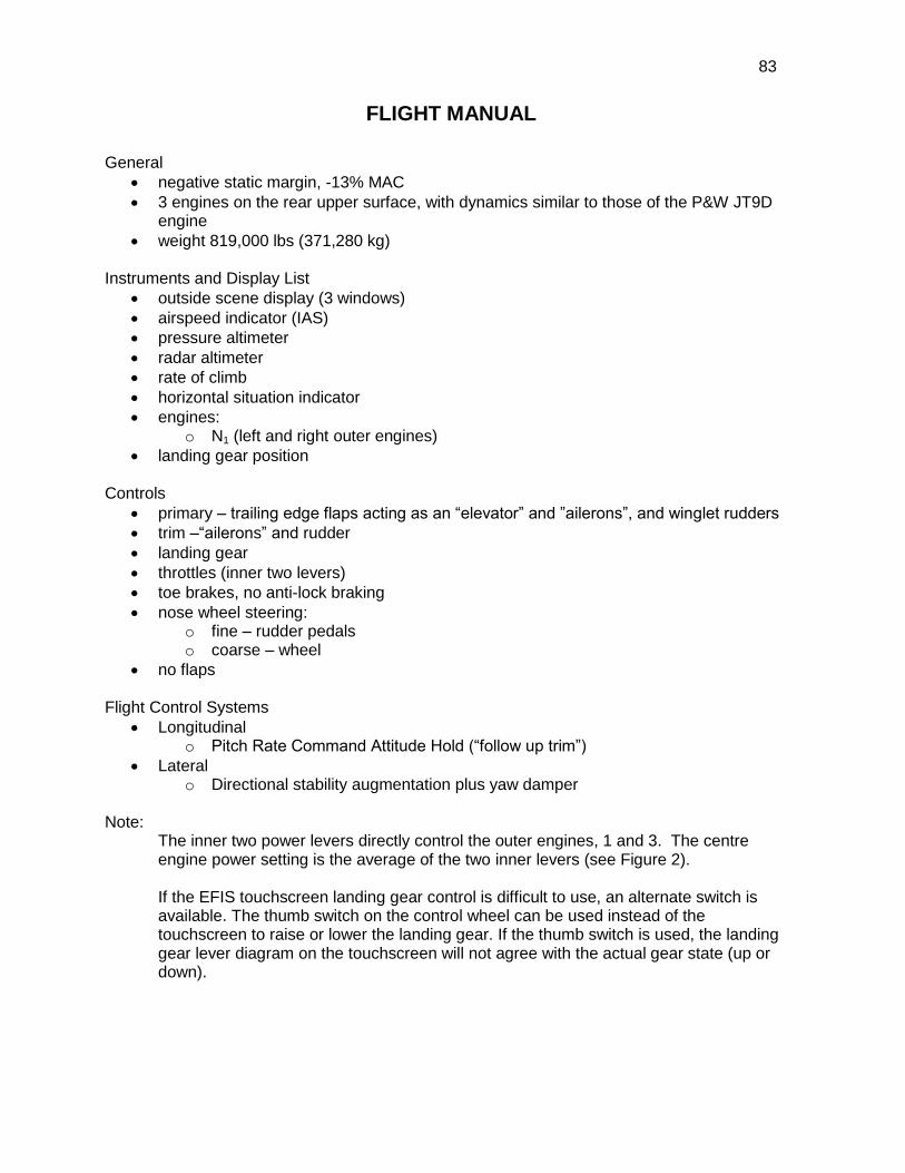
83

FLIGHT MANUAL

General

negative static margin, -13% MAC

3 engines on the rear upper surface, with dynamics similar to those of the P&W JT9D engine

weight 819,000 lbs (371,280 kg) Instruments and Display List

outside scene display (3 windows)

airspeed indicator (IAS)

pressure altimeter

radar altimeter

rate of climb

horizontal situation indicator

engines: o N1 (left and right outer engines)

landing gear position Controls

primary – trailing edge flaps acting as an “elevator” and ”ailerons”, and winglet rudders

trim –“ailerons” and rudder

landing gear

throttles (inner two levers)

toe brakes, no anti-lock braking

nose wheel steering: o fine – rudder pedals o coarse – wheel

no flaps Flight Control Systems

Longitudinal o Pitch Rate Command Attitude Hold (“follow up trim”)

Lateral o Directional stability augmentation plus yaw damper

Note:

The inner two power levers directly control the outer engines, 1 and 3. The centre engine power setting is the average of the two inner levers (see Figure 2). If the EFIS touchscreen landing gear control is difficult to use, an alternate switch is available. The thumb switch on the control wheel can be used instead of the touchscreen to raise or lower the landing gear. If the thumb switch is used, the landing gear lever diagram on the touchscreen will not agree with the actual gear state (up or down).

84

COOPER HARPER SCALE

Documents

Handling Qualities of a Blended Wing Body Aircraft Handling Qualities of a Blended Wing Body Aircraft Timothy Shaw Peterson Master of Applied Science Institute for Aerospace Studies