Hamiltonian Partial Differential Equations

James Colliander

University of Toronto

2011-10-04, Edinburgh

Dynamical systems and classical mechanics: a conference incelebration of Vladimir Arnold 1937 - 2010

1 Introduction

2 Cauchy Problem

3 Critical Scattering

4 Turbulence

5 Conclusion

1. Introduction

1. Introduction

Hamiltonian PDE?

PDEs vs. ODEsIntegrable vs NonintegrableFocusing vs. DefocusingBounded vs. Unbounded spatial domain

Dynamics exploring infinite dimensional phase space?

Low-to-high frequency cascadeSingularity formation

Survey recent advances; highlight research directions.

Mostly discuss defocusing NLSSeveral interesting threads omitted

2. Cauchy Problem

2. Cauchy Problem

Consider the defocusing monomial NLS initial value problem:{(i∂t + ∆)u = |u|p−1u

u(0, x) = u0(x).(NLS+

p (Rd))

Time invariant quantitites:

Mass =

∫T|u(t, x)|2dx.

Momentum = 2=∫T

u(t)∂xu(t)dx.

Energy = H[u(t)] =

∫T

12|∂xu(t)|2dx +

2p + 1

|u(t)|p+1dx.

Dilation Invariance

u : [0,T]× Rd 7−→ C solves NLS+p (Rd)

m∀ λ > 0, uλ : [0, λ2T]× Rd] 7−→ C solves NLS+

p (Rd)

whereuλ(τ, y) = (

1λ

)2

p−1 u(τ

λ2 ,yλ

).

A simple calculation shows that

‖Dsuλ(τ, ·)‖L2 = (1λ

)2

p−1 +s− d2 ‖Dsu(τ)‖L2 .

We encounter a dilation invariant Sobolev space norm when

s = sc =d2− 2

p− 1.

The space Hsc(Rd) plays a basic role in theory for NLSp(Rd).

Criticality Regimes NLS+p (Rd)

Recall the critical Sobolev regularity index for NLS+p (Rd):

s = sc =d2− 2

p− 1.

Conservation laws identify 5 critical regimes:sc < 0, Mass Subcriticalsc = 0, Mass Critical0 < sc < 1, Mass Supercritical/Energy Subcrticalsc = 1, Energy Criticalsc > 1, Energy Supercritical.

Global Wellposedness for Energy Subcritical Regime

H1-Local Wellposedness Lifetime depends on H1 norm:

Tlwp ∼ ‖u(0)‖−γH1 .

Energy Conservation implies H1 a priori control:

‖u(t)‖2H1 ≤ Energy[u(0)], ∀ t.

Iterate the local theory with uniform time steps =⇒ GWP.

Remarks:

Maximal-in-time behavior of solutions? Not clear...Low regularity relaxations (high/low frequency, I-method)Polynomial in time bounds on ‖u(t)‖Hs , s� 1.

GWP for Energy Critical Regime

LWP iteration FAILS:

Energy implies H1 a priori control:‖u(t)‖2H1 ≤ Energy[u(0)].

H1-LWP lifetime not controlled by H1 norm.H1-LWP iteration does NOT imply GWP.

Question: What happens maximally in time?

3. Energy Critical Scattering

3. Energy Critical Scattering

New ideas have completely resolved energy critical NLS.

GWP for large H1 data is now known.Long-time behavior is understood: Scattering∀ u0 ∈ H1(R3) ∃ u± ∈ H1 such that for NLS+

5 (R3)

limt→±∞

‖u(t)− e±it∆u±‖H1 = 0,

and‖u‖L10(Rt×R3

x) ≤ C(u0).

Induction on Energy

Induction on Energy Approach [Bou99]NLS+

5 (R3), NLS+3 (R4) radial.

NLS+5 (R3) GWP and Scatters [CKS+08].

4 and higher dimensions [RV07], [Vis10].

Induction on Energy Idea

Monotonicity

The discussion which follows is a quantum (and nonlinear)generalization of a Lyapunov functional discussed in A.Shnirelman’s lecture.

Generalized Virial Identity

Let a : Rd → R (virial weight). Form the virial potential

Va(t) =

∫Rd

a(x)|φ(t, x)|2dx.

Form the Morawetz action

Ma(t) =

∫Rd∇a · 2=(φ∇φ)dx.

Conservation identities lead to the generalized virial identities

∂tVa = Ma +

∫Rd

a(x){N , φ}m(t, x)dx,

∂tMa =

∫Rd

(−∆∆a)|φ|2 + 4ajk<(φjφk) + 2aj{N , φ}jpdx.

Remarks on Virial Identities

The virial potential is a weighted average of the massdensity against the virial weight a.The Morawetz action is a contraction of the momentumdensity against∇a. Vector fields not arising as gradientscould also be considered.Useful estimates emerge from monotonicity andboundedness of terms in the virial identities.Monotone quantities provide dynamical insights.Idea of Morawetz Estimates: Cleverly choose the weightfunction a so that ∂tMa ≥ 0 but Ma ≤ C(φ0) to obtainspacetime control on φ. This strategy imposes variousconstraints on a which suggest choosing a(x) = |x|.

Variance Identity

[Gla77], [Vlasov-Petrischev-Talanov]

Consider GNLS with N = ±|u|4/du. This is the L2 criticalfocusing equation NLS±

1+ 4d(Rd).

Choose a(x) = |x|2. Calculations reveal that

∂2t

∫Rd|x|2|u(t, x)|2dx = 16H[u(t)].

In the focusing case, we can consider initial data u0 withH[u0] < 0 and finite variance. Such data must blow up infinite time.

[Lin-Strauss] Morawetz identity

Consider (i∂t + ∆)φ = F′(|φ|2)φ with F′ ≥ 0 and x ∈ R3. Choosea(x) = |x|. Observe that a is weakly convex,∇a = x

|x| isbounded, and −∆∆a = 4πδ0. From monotonicity ∂tMa ≥ 0 andthe bound |Ma| ≤

√H[u0] emerges the Lin-Strauss Morawetz

identity

Ma(T)−Ma(0) =

T∫0

∫R3

4πδ0(x)|φ(t, x)|2 + (≥ 0) + 4G(|φ|2)

|x|dxdt.

This implies the spacetime control estimate (centered at x = 0)

(H[u0])1/2‖u0‖L2 &

T∫0

∫R3

G(|φ|2)

|x|dxdt.

Averaging over [Lin-Strauss] center?

Translation invariance? Weight |x|−1 difficult in proofs.Recenter [L-S] at fixed y ∈ Rd. Set a(x) = |x− y|.Recentered Morawetz action can be expressed

My[u](t) =

∫Rd

(x− y)

|x− y|2=(u∇u)(t, x)dx.

Monotonicity ∂tMy[u] ≥ 0: mass is repelled from anyy ∈ Rd.Can we average with respect to center y and obtain newtranslation invariant spacetime control?Yes, if we average against the natural density |u(t, y)|2.

Interaction Morawetz via Averaging

Define the Morawetz interaction potential

M[u](t) =

∫Rd

y

|u(t, y)|2My[u](t)dy.

It is bounded:∣∣∣M[u](t)

∣∣∣ . ‖u(t)‖3L2

x‖∇u(t)‖L2

x. We calculate

∂tM[u] =

∫Rd

y

|u(t, y)|2{∂tMy[u]}+ {∂t|u(y)|2}My[u]dy.

Local conservation & [L-S] =⇒ monotonicity:∃ I, II, III, IV such that I, III ≥ 0 and II + IV ≥ 0 and∂tM[u] = I + II + III + IV. Integrating in time gives∫ T

0

∫R3|u(t, x)|4dxdt . ‖u(t)‖3

L∞T L2x‖∇u(t)‖L∞T L2

x.

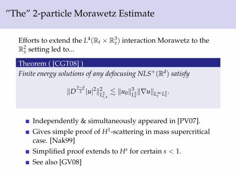
”The” 2-particle Morawetz Estimate

Efforts to extend the L4(Rt × R3x) interaction Morawetz to the

R2x setting led to...

Theorem ( [CGT08] )Finite energy solutions of any defocusing NLS+(Rd) satisfy

‖D3−d

2 |u|2‖2L2

t,x. ‖u0‖3

L2x‖∇u‖L∞t L2

x.

Independently & simultaneously appeared in [PV07].Gives simple proof of H1-scattering in mass supercriticalcase. [Nak99]Simplified proof extends to Hs for certain s < 1.See also [GV08]

Frequency Barriers

Critical Elements Method

Extract critical elements then kill them:

Relaxed approach developed by Kenig-Merle [KM08].Avoids quantitative perturbation theory.Uses compactness (modulo symmetries) tools instead.”Profile Decompositions” [Ker01]

Robust Method:

Progress on focusing problems beneath soliton threshold.Mass Critical Case [Dod10]Other equations, including Navier-Stokes [KK09]Recent progress on compact and product domains. [IP11]

Energy Supercritical Maximal-in-time Theory?

This theory is wide open.We have no a priori control on Sobolev norms with s > 1.Same issue obstructs Navier-Stokes initial value problem?

Critical Norm Bounded =⇒ Scattering

Bounded Hsc norm Assumption: Suppose Hsc 3 u(0) 7−→ usolves NLS or NLW with sc > 1 and ∃ K < 0 such that

supt‖u(t)‖Hsc < K.

NLWp(Rd):Radial + Bounded Hsc norm =⇒ scattering [KM10],[KM08].NLS+

p (Rd): Bounded Hsc norm =⇒ scattering[Killip-Visan 2009].

Question: What is the behavior of ‖u(t)‖Hsc ?

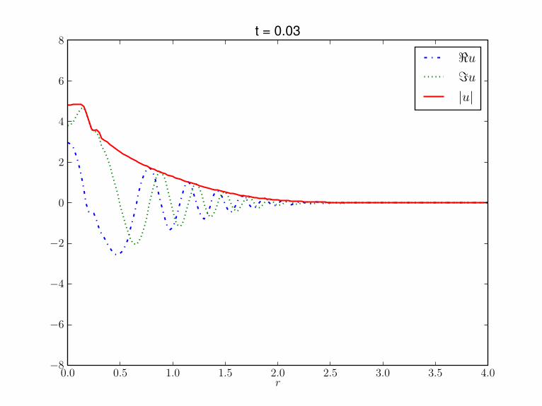
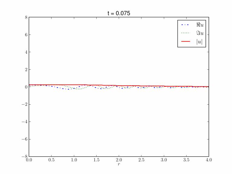
Numerical Simulations of Supercritical Waves

Strauss-Vazquez simulated NLW [SV78].NLS+

5 (R5) observed to have bounded H2 norm [CSS09].

0.0 0.5 1.0 1.5 2.0 2.5 3.0 3.5 4.0r

−8

−6

−4

−2

0

2

4

6

8t = 0

<u=u|u|

0.0 0.5 1.0 1.5 2.0 2.5 3.0 3.5 4.0r

−8

−6

−4

−2

0

2

4

6

8t = 0.005

<u=u|u|

0.0 0.5 1.0 1.5 2.0 2.5 3.0 3.5 4.0r

−8

−6

−4

−2

0

2

4

6

8t = 0.01

<u=u|u|

0.0 0.5 1.0 1.5 2.0 2.5 3.0 3.5 4.0r

−8

−6

−4

−2

0

2

4

6

8t = 0.015

<u=u|u|

0.0 0.5 1.0 1.5 2.0 2.5 3.0 3.5 4.0r

−8

−6

−4

−2

0

2

4

6

8t = 0.02

<u=u|u|

0.0 0.5 1.0 1.5 2.0 2.5 3.0 3.5 4.0r

−8

−6

−4

−2

0

2

4

6

8t = 0.025

<u=u|u|

0.0 0.5 1.0 1.5 2.0 2.5 3.0 3.5 4.0r

−8

−6

−4

−2

0

2

4

6

8t = 0.03

<u=u|u|

0.0 0.5 1.0 1.5 2.0 2.5 3.0 3.5 4.0r

−8

−6

−4

−2

0

2

4

6

8t = 0.035

<u=u|u|

0.0 0.5 1.0 1.5 2.0 2.5 3.0 3.5 4.0r

−8

−6

−4

−2

0

2

4

6

8t = 0.04

<u=u|u|

0.0 0.5 1.0 1.5 2.0 2.5 3.0 3.5 4.0r

−8

−6

−4

−2

0

2

4

6

8t = 0.045

<u=u|u|

0.0 0.5 1.0 1.5 2.0 2.5 3.0 3.5 4.0r

−8

−6

−4

−2

0

2

4

6

8t = 0.05

<u=u|u|

0.0 0.5 1.0 1.5 2.0 2.5 3.0 3.5 4.0r

−8

−6

−4

−2

0

2

4

6

8t = 0.055

<u=u|u|

0.0 0.5 1.0 1.5 2.0 2.5 3.0 3.5 4.0r

−8

−6

−4

−2

0

2

4

6

8t = 0.06

<u=u|u|

0.0 0.5 1.0 1.5 2.0 2.5 3.0 3.5 4.0r

−8

−6

−4

−2

0

2

4

6

8t = 0.065

<u=u|u|

0.0 0.5 1.0 1.5 2.0 2.5 3.0 3.5 4.0r

−8

−6

−4

−2

0

2

4

6

8t = 0.07

<u=u|u|

0.0 0.5 1.0 1.5 2.0 2.5 3.0 3.5 4.0r

−8

−6

−4

−2

0

2

4

6

8t = 0.075

<u=u|u|

0.0 0.5 1.0 1.5 2.0 2.5 3.0 3.5 4.0r

−8

−6

−4

−2

0

2

4

6

8t = 0.08

<u=u|u|

0.0 0.5 1.0 1.5 2.0 2.5 3.0 3.5 4.0r

−8

−6

−4

−2

0

2

4

6

8t = 0.085

<u=u|u|

0.0 0.5 1.0 1.5 2.0 2.5 3.0 3.5 4.0r

−8

−6

−4

−2

0

2

4

6

8t = 0.09

<u=u|u|

0.0 0.5 1.0 1.5 2.0 2.5 3.0 3.5 4.0r

−8

−6

−4

−2

0

2

4

6

8t = 0.095

<u=u|u|

0.0 0.5 1.0 1.5 2.0 2.5 3.0 3.5 4.0r

−8

−6

−4

−2

0

2

4

6

8t = 0.1

<u=u|u|

0 50 100 150 200k

10−22

10−20

10−18

10−16

10−14

10−12

10−10

10−8

10−6

10−4

10−2 |u(k)|(t = 0)

|u(k)|(t = 0.01)

|u(k)|(t = 0.02)

|u(k)|(t = 0.04)

|u(k)|(t = 0.1)

0.00 0.02 0.04 0.06 0.08 0.10t

600

650

700

750

800

850‖∆

u‖ L

2

0.00 0.02 0.04 0.06 0.08 0.10t

600

650

700

750

800

850‖∆

u‖ L

2

0.00 0.02 0.04 0.06 0.08 0.100.50

0.52

0.54

0.56

0.58

0.60

0.62

0.64

0.66

0.68

‖u‖ B

2 2,∞

0.00 0.02 0.04 0.06 0.08 0.10t

0.0

0.5

1.0

1.5

2.0

2.5

3.0

3.5‖u‖ L

6

4. Turbulence

The NLS Initial Value Problem

We [CKS+10] consider the defocusing initial value problem:{(−i∂t + ∆)u = |u|2u

u(0, x) = u0(x), where x ∈ T2.(NLS(T2))

Smooth solution u(x, t) exists globally and

Mass = M(u) = ‖u(t)‖2 = M(0)

Energy = E(u) =

∫(12|∇u(t, x)|2 +

14|u(x, t)|4) dx = E(0)

We want to understand the shape of |u(t, ξ)|. The conservationlaws impose L2-moment constraints on this object.

Notion of Frequency Cascade

Definition

A frequency cascade is the phenomenon of global-in-timesolutions shifting their mass toward increasingly highfrequencies.

This shift is also called a forward cascade.A way to measure the cascade is to study

‖u(t)‖2Hs =

∫|u(t, ξ)|2|ξ|2sdξ

and prove that it grows for large times t.The cascade is incompatible with scattering andintegrability.

Incompatible with Scattering & Integrability

Scattering: ∀ global solution u(t, x) ∈ Hs ∃ u+0 ∈ Hs with,

limt→+∞

‖u(t, x)− eit∆u+0 (x)‖Hs = 0.

Note: ‖eit∆u+0 ‖Hs = ‖u+

0 ‖Hs =⇒ ‖u(t)‖Hs is bounded.Complete Integrability: The 1d equation

(i∂t + ∆)u = −|u|2u

has infinitely many conservation laws. Combining them inthe right way one gets that ‖u(t)‖Hn ≤ Cn for all times.

Past Results

Bourgain: (late 90’s) [Bou98]For the periodic IVP NLS(T2) one can prove

‖u(t)‖2Hs ≤ Cs|t|4s.

The idea is to improve the local estimate for t ∈ [−1, 1]

‖u(t)‖Hs ≤ Cs‖u(0)‖Hs , for Cs � 1

( =⇒ ‖u(t)‖Hs . C|t| upper bounds) to obtain

‖u(t)‖Hs ≤ 1‖u(0)‖Hs + Cs‖u(0)‖1−δHs for Cs � 1,

for some δ > 0. This iterates to give

‖u(t)‖Hs ≤ Cs|t|1/δ.

Improvements: [Sta97], [CDKS01].

Past Results

Bourgain: (late 90’s)Given m, s� 1 there exist ∆ and a global solution u(x, t) to

(∂tt − ∆)u = up

such that ‖u(t)‖Hs ∼ |t|m.Physics: Weak turbulence theory: Hasselmann [Has62] &[Zakharov] .Numerics (d=1): [MMT97]Kuksin [Kuk97] has studied a small dispersion NLS

i∂tw + δ∆w = |w|2w

with 0 < δ � 1. Smooth norms of relatively generic data,with unit sized L2 norm, are shown to grow larger than anegative power of δ. These results correspond to large datasolutions of the δ = 1 problem NLS+

3 (T2).

Exploding Sobolev Norms Conjecture?

Solutions to dispersive equations on Rd have boundedhigh Sobolev norms.There are solutions to nonlinear dispersive equations on Td

with exploding Sobolev norms. In particular for NLS(T2)there exists u(t, x) such that

‖u(t)‖2Hs →∞ as t→∞.

The cascade phenomena of high Sobolev norm explosionshould be generic in phase space.

Main Result

We consider the defocusing initial value problem:{(−i∂t + ∆)u = |u|2u

u(0, x) = u0(x), where x ∈ T2.(NLS(T2))

Theorem ([CKS+10])Let s > 1, K� 1 and 0 < σ < 1 be given. Then there exists a globalsmooth solution u(t, x) and T > 0 such that

‖u0‖Hs ≤ σ

and‖u(t)‖2

Hs ≥ K.

See also recent thesis [Zaher Hani].

Origin of Proof

4 frequency exampleMove energy from 1 and i to 0 and 1 + iLeverage

√2 > 1.

Preliminary reductions

Gauge Freedom:If u solves NLS then v(t, x) = e−i2Gtu(t, x) solves{

i∂tv + ∆v = (2G + |v|2)vv(0, x) = v0(x), x ∈ T2.

(NLSG)

Fourier Ansatz: Recast the dynamics in Fouriercoefficients,

v(t, x) =∑n∈Z2

an(t)ei(n·x+|n|2t).

i∂tan = 2Gan +

∑n1,n2,n3 ∈ Z2

n1 − n2 + n3 = n

an1an2an3eiω4t

an(0) = u0(n), n ∈ Z2.(FNLSG)

ω4 = |n1|2 − |n2|2 + |n3|2 − |n|2.

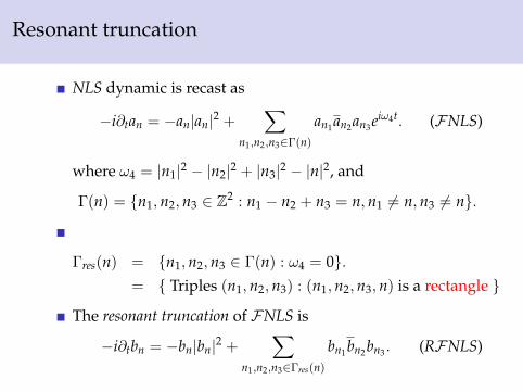
Resonant truncation

NLS dynamic is recast as

−i∂tan = −an|an|2 +∑

n1,n2,n3∈Γ(n)

an1an2an3eiω4t. (FNLS)

where ω4 = |n1|2 − |n2|2 + |n3|2 − |n|2, and

Γ(n) = {n1,n2,n3 ∈ Z2 : n1 − n2 + n3 = n,n1 6= n,n3 6= n}.

Γres(n) = {n1,n2,n3 ∈ Γ(n) : ω4 = 0}.= { Triples (n1,n2,n3) : (n1,n2,n3,n) is a rectangle }

The resonant truncation of FNLS is

−i∂tbn = −bn|bn|2 +∑

n1,n2,n3∈Γres(n)

bn1bn2bn3 . (RFNLS)

Finite dimensional resonant restriction

A set Λ ⊂ Z2 is closed under resonant interactions if

n1,n2,n3 ∈ Γres(n),n1,n2,n3 ∈ Λ =⇒ n ∈ Λ.

A finite dimensional resonant restriction of FNLS is

−i∂tbn = −bn|bn|2 +∑

n1,n2,n3∈Γres(n)∩Λ3

bn1bn2bn3 . (RFNLSΛ)

∀ resonant-closed finite Λ ⊂ Z2 RFNLSΛ is an ODE.If spt(an(0)) ⊂ Λ then FNLS-evolution an(0) 7−→ an(t) isnicely approximated by RFNLSΛ-ODE an(0) 7−→ bn(t).Given ε, s,K, build Λ so that RFNLSΛ cascades.

Imagine we build a resonant Λ ⊂ Z2 such that...

Imagine a resonant-closed Λ = Λ1 ∪ · · · ∪ ΛM with properties.Define a nuclear family to be a rectangle (n1,n2,n3,n4) wherethe frequencies n1,n3 (the ’parents’) live in generation Λj andn2,n4 (’children’) live in generation Λj+1.

∀ 1 ≤ j < M and ∀ n1 ∈ Λj ∃ unique nuclear family suchthat n1,n3 ∈ Λj are parents and n2,n4 ∈ Λj+1 are children.∀ 1 ≤ j < M and ∀ n2 ∈ Λj+1 ∃ unique nuclear family suchthat n2,n4 ∈ Λj+1 are children and n1,n3 ∈ Λj are parents.The sibling of a frequency is never its spouse.Besides nuclear families, Λ contains no other rectangles.The function n 7−→ an(0) is constant on each generation Λj.

Cartoon Construction of Λ

Cartoon Construction of Λ

Cartoon Construction of Λ

Cartoon Construction of Λ

Cartoon Construction of Λ

Cartoon Construction of Λ

Cartoon Construction of Λ

Cartoon Construction of Λ

Cartoon Construction of Λ

Cartoon Construction of Λ

Cartoon Construction of Λ

Cartoon Construction of Λ

Cartoon Construction of Λ

Cartoon Construction of Λ

Cartoon Construction of Λ

Cartoon Construction of Λ

The toy model ODE

Assume we can construct such a Λ = Λ1 ∪ · · · ∪ ΛM. Theproperties imply RFNLSΛ simplifies to the toy model ODE

∂tbj(t) = −i|bj(t)|2bj(t) + 2ibj(t)[bj−1(t)2 + bj+1(t)2].

L2 ∼∑

j

|bj(t)|2 =∑

j

|bj(0)|2

Hs ∼∑

j

|bj(t)|2(∑n∈Λj

|n|2s).

We also want Λ to satisfy Wide Diaspora Property∑n∈ΛM

|n|2s �∑n∈Λ1

|n|2s.

Conservation laws for the ODE system

Mass =∑

j

|bj(t)|2 = C0

Momentum =∑

j

|bj(t)|2∑n∈Λj

n = C1,

Energy = K + P = C2,

where

K =∑

j

|bj(t)|2∑n∈Λj

|n|2,

P =12

∑j

|bj(t)|4 +∑

j

|bj(t)|2|bj+1(t)|2.

Conservation laws for ODE do not involve Fourier moments!

Concatenated Sliders for Toy Model ODE

Using dynamical systems methods, we construct a Toy ModelODE evolution such that:

Concatenated Sliders for Toy Model ODE

Using dynamical systems methods, we construct a Toy ModelODE evolution such that:

A travelling wave through the generations.

Properties of the Toy Model ODE

Solution of the Toy Model is a vector flow t→ b(t) ∈ CM

b(t) = (b1(t), . . . , bM(t)) ∈ CM; bj = 0 ∀ j ≤ 0, j ≥M + 1.

Local Well-Posedness; Let S(t) denote associated flowmap.Mass Conservation: |b(t)|2 = |b(0)|2 =⇒

Toy Model ODE is Globally Well-Posed.Invariance of the sphere: Σ = {x ∈ CM : |x|2 = 1}

S(t)Σ = Σ.

Properties of the Toy Model ODE

Support Conservation:

∂t|bj|2 = 2Re(bj∂tbj)

= 4Re(ibj2[b2

j−1 + b2j+1])

≤ 4|bj|2.

Thus, if bj(0) = 0 then bj(t) = 0 for all t.Invariance of coordinate tori:

Tj = {(b1, . . . , bM ∈ Σ) : |bj| = 1, bk = 0 ∀ k 6= j}

Mass Conservation =⇒ S(T)Tj = Tj.Dynamics on the invariant tori is easy:

bj(t) = e−i(t+θ); bk(t) = 0 ∀ k 6= j.

Explicit Slider Solutions

Consider M = 2. Then ODE is of the form

∂tb1 = −i|b1|2b1 + 2ib1b22

∂tb2 = −i|b2|2b2 + 2ib2b21.

Let ω = e2iπ/3 (cube root of unity). This ODE has explicitsolution

b1(t) =e−it√

1 + e2√

3tω , b2(t) =

e−it√1 + e−2

√3tω2.

As t→ −∞, (b1(t), b2(t))→ (e−itω, 0) ∈ T1.As t→ +∞, (b1(t), b2(t))→ (0, e−itω2) ∈ T2.

Two Explicit Solution Families

Tj T1 T2

Concatenated Sliders: Idea of Proof

5. Conclusion

A quotation

V.I. Arnold ”On A.N. Kolmogorov” in the book Kolmgorov inPerspective, 2000.

”One can distinguish three stages on the development ofany new area of science. The first is the pioneering stage:the breakthrough into a new area, a striking and usuallyunexpected discovery, often running counter to establishednotions. Then follows the technical stage which is long andlaborious. The theory is overgrown with details, it becomescumbersome and difficult to understand, but in return itencompasses an ever greater number of applications.Finally, in the third stage there emerges a new and moregeneral view of the problem and of its connections withother questions apparently remote from it: a breakthroughinto a new area of research has been made possible”

References

Jean Bourgain, Refinements of Strichartz’ inequality andapplications to 2D-NLS with critical nonlinearity, InternationalMathematics Research Notices (1998), no. 5, 253283.

, Global wellposedness of defocusing critical nonlinearschr\”odinger equation in the radial case, Journal of theAmerican Mathematical Society 12 (1999), no. 1, 145171.

J. E Colliander, J. -M Delort, C. E Kenig, and G. Staffilani,Bilinear estimates and applications to 2D NLS, Transactions ofthe American Mathematical Society 353 (2001), no. 8,33073325 (electronic).

Jim Colliander, Manoussos Grillakis, and NikolaosTzirakis, Tensor products and correlation estimates withapplications to nonlinear schr\”odinger equations, 0807.0871(2008).

J. Colliander, M. Keel, G. Staffilani, H. Takaoka, and T. Tao,Global well-posedness and scattering for the energy-criticalnonlinear Schr\”odinger equation in $\mathbbrˆ3$, Annals ofMathematics. Second Series 167 (2008), no. 3, 767865.

, Transfer of energy to high frequencies in the cubicdefocusing nonlinear Schr\”odinger equation, InventionesMathematicae 181 (2010), no. 1, 39113.

James Colliander, Gideon Simpson, and Catherine Sulem,Numerical simulations of the energy- supercritical nonlinearSchr\”odinger equation, arXiv math.AP (2009), 17 pages with9 figures.

Benjamin Dodson, Global well-posedness and scattering for thedefocusing, $lˆ2$-critical, nonlinear schr\”odinger equationwhen $d = 1$, 1010.0040 (2010).

R. T. Glassey, On the blowing up of solutions to the cauchyproblem for nonlinear schrdinger equations, Journal ofMathematical Physics 18 (1977), no. 9, 17941797.

J. Ginibre and G. Velo, Quadratic Morawetz inequalities andasymptotic completeness in the energy space for nonlinearSchr\”odinger and Hartree equations, arXiv math.AP (2008).

K. Hasselmann, On the non-linear energy transfer in agravity-wave spectrum. i. General theory, Journal of FluidMechanics 12 (1962), 481500.

A. D Ionescu and B. Pausader, The energy-critical defocusingNLS on $\mathbbtˆ3$, arXiv:1102.5771 (2011).

Sahbi Keraani, On the defect of compactness for the Strichartzestimates of the Schr\”odinger equations, Journal ofDifferential Equations 175 (2001), no. 2, 353392.

Carlos E Kenig and Gabriel Koch, An alternative approach toregularity for the Navier-Stokes equations in a critical space,Arxiv preprint arXiv:0908.3349 (2009).

Carlos E Kenig and Frank Merle, Nondispersive radialsolutions to energy supercritical non-linear wave equations, withapplications, 0810.4834 (2008).

, Scattering for $hˆ1/2$ bounded solutions to the cubic,defocusing NLS in 3 dimensions, Trans. Amer. Math. Soc. 362(2010), no. 4, 19371962.

S. B. Kuksin, On turbulence in nonlinear schrdinger equations,Geometric and Functional Analysis 7 (1997), no. 4, 783822.

A. J. Majda, D. W. McLaughlin, and Esteban Tabak, Aone-dimensional model for dispersive wave turbulence, Journalof Nonlinear Science 7 (1997), no. 1, 944.

Kenji Nakanishi, Energy scattering for nonlinear Klein-Gordonand Schr\”odinger equations in spatial dimensions $1$ and $2$,Journal of Functional Analysis 169 (1999), no. 1, 201225.

Fabrice Planchon and Luis Vega, Bilinear virial identities andapplications, 0712.4076 (2007).

E. Ryckman and M. Visan, Global well-posedness andscattering for the defocusing energy-critical nonlinearSchr\”odinger equation in $\mathbbrˆ1+4$, American Journalof Mathematics 129 (2007), no. 1, 160.

Gigliola Staffilani, On the growth of high Sobolev norms ofsolutions for KdV and schr\”odinger equations, DukeMathematical Journal 86 (1997), 109–142.

Walter Strauss and Luis Vazquez, Numerical solution of anonlinear Klein-Gordon equation, Journal of ComputationalPhysics 28 (1978), no. 2, 271278.

Monica Visan, Global well-posedness and scattering for thedefocusing cubic NLS in four dimensions, 1011.1526 (2010).