Embed Size (px)
Citation preview


0
1
2
3
4
5
6
7
8
9
10
11
12
13
14
15
16
Table of ContentsIntroduction
What is H2O?
Intro to Data Science
Building a Smarter Application
Deep Learning
GBM & Random Forest
GLM
GLRM
AutoML
NLP with H2O
Hive UDF POJO Example
Hive UDF MOJO Example
Ensembles: Stacking, Super Learner
Streaming
Sparkling Water
PySparkling
Resources
H2O TutorialsThis document contains tutorials and training materials for H2O-3. Post questions on StackOverflow using the h2o tag athttp://stackoverflow.com/questions/tagged/h2o or join the "H2O Stream" Google Group:
Web: https://groups.google.com/forum/#!forum/h2ostreamE-mail: [email protected]
Finding tutorial material in Github
Most current material
Tutorials in the master branch are intended to work with the lastest stable version of H2O.
URL
Training material https://github.com/h2oai/h2o-tutorials/blob/master/SUMMARY.md
Latest stable H2O release http://h2o.ai/download
Historical events
Tutorial versions in named branches are snapshotted for specific events. Scripts should work unchanged for the version of H2O used atthat time.
H2O World 2017 Training
URL
Training material https://github.com/h2oai/h2o-tutorials/tree/master/h2o-world-2017/README.md
Wheeler-2 H2O release http://h2o-release.s3.amazonaws.com/h2o/rel-wheeler/2/index.html
H2O World 2015 Training
URL
Training material https://github.com/h2oai/h2o-tutorials/blob/h2o-world-2015-training/SUMMARY.md
Tibshirani-3 H2O release http://h2o-release.s3.amazonaws.com/h2o/rel-tibshirani/3/index.html
R Tutorials
Intro to H2O in RH2O Grid Search & Model SelectionH2O Deep Learning in RH2O Stacked Ensemblesh2oEnsemble R package
Python Tutorials
Intro to H2O in PythonH2O Grid Search & Model SelectionH2O Stacked Ensembles
For most tutorials using python you can install dependent modules to your environment by running the following commands.
# As current user
pip install -r requirements.txt
# As root user
sudo -E pip install -r requirements.txt
Note: If you are behind a corporate proxy you may need to set environment variables for https_proxy accordingly.
# If you are behind a corporate proxy
export https_proxy=https://<user>:<password>@<proxy_server>:<proxy_port>
# As current user
pip install -r requirements.txt
# If you are behind a corporate proxy
export https_proxy=https://<user>:<password>@<proxy_server>:<proxy_port>
# As root user
sudo -E pip install -r requirements.txt

What is H2O?H2O is fast, scalable, open-source machine learning and deep learning for Smarter Applications. With H2O, enterprises like PayPal,Nielsen Catalina, Cisco and others can use all of their data without sampling and get accurate predictions faster. Advanced algorithms, likeDeep Learning, Boosting, and Bagging Ensembles are readily available for application designers to build smarter applications throughelegant APIs. Some of our earliest customers have built powerful domain-specific predictive engines for Recommendations, CustomerChurn, Propensity to Buy, Dynamic Pricing and Fraud Detection for the Insurance, Healthcare, Telecommunications, AdTech, Retail andPayment Systems.
Using in-memory compression techniques, H2O can handle billions of data rows in-memory, even with a fairly small cluster. The platformincludes interfaces for R, Python, Scala, Java, JSON and Coffeescript/JavaScript, along with a built-in web interface, Flow, that make iteasier for non-engineers to stitch together complete analytic workflows. The platform was built alongside (and on top of) both Hadoop andSpark Clusters and is typically deployed within minutes.
H2O implements almost all common machine learning algorithms, such as generalized linear modeling (linear regression, logisticregression, etc.), Naïve Bayes, principal components analysis, time series, k-means clustering, and others. H2O also implements best-in-class algorithms such as Random Forest, Gradient Boosting, and Deep Learning at scale. Customers can build thousands of models andcompare them to get the best prediction results.
H2O is nurturing a grassroots movement of physicists, mathematicians, computer and data scientists to herald the new wave of discoverywith data science. Academic researchers and Industrial data scientists collaborate closely with our team to make this possible. Stanforduniversity giants Stephen Boyd, Trevor Hastie, Rob Tibshirani advise the H2O team to build scalable machine learning algorithms. With100s of meetups over the past two years, H2O has become a word-of-mouth phenomenon growing amongst the data community by a 100-fold and is now used by 12,000+ users, deployed in 2000+ corporations using R, Python, Hadoop and Spark.
Try it out
H2O offers an R package that can be installed from CRAN, and a python package that can be installed from PyPI.
H2O can also be downloaded directly from http://h2o.ai/download.
Join the community
Visit the open source community forum at https://groups.google.com/d/forum/h2ostream.
To learn about our meetups, training sessions, hackathons, and product updates, visit http://h2o.ai.

Intro to Data Science
Slides
PDFKeynote

Building a Smarter Application
Slides
PDFPowerPoint
Code
The source code for this example is here: https://github.com/h2oai/app-consumer-loan
Classification and Regression with H2O Deep LearningIntroduction
Installation and StartupDecision Boundaries
Cover Type DatasetExploratory Data AnalysisDeep Learning ModelHyper-Parameter SearchCheckpointingCross-ValidationModel Save & Load
Regression and Binary ClassificationDeep Learning Tips & Tricks
IntroductionThis tutorial shows how a H2O Deep Learning model can be used to do supervised classification and regression. A great tutorial aboutDeep Learning is given by Quoc Le here and here. This tutorial covers usage of H2O from R. A python version of this tutorial will beavailable as well in a separate document. This file is available in plain R, R markdown and regular markdown formats, and the plots areavailable as PDF files. All documents are available on Github.
If run from plain R, execute R in the directory of this script. If run from RStudio, be sure to setwd() to the location of this script. h2o.init()starts H2O in R's current working directory. h2o.importFile() looks for files from the perspective of where H2O was started.
More examples and explanations can be found in our H2O Deep Learning booklet and on our H2O Github Repository. The PDF slidedeck can be found on Github.
H2O R Package
Load the H2O R package:
## R installation instructions are at http://h2o.ai/download
library(h2o)
Start H2O
Start up a 1-node H2O server on your local machine, and allow it to use all CPU cores and up to 2GB of memory:
h2o.init(nthreads=-1, max_mem_size="2G")
h2o.removeAll() ## clean slate - just in case the cluster was already running
The h2o.deeplearning function fits H2O's Deep Learning models from within R. We can run the example from the man page using the example function, or run a longer demonstration from the h2o package using the demo function:
args(h2o.deeplearning)
help(h2o.deeplearning)
example(h2o.deeplearning)
#demo(h2o.deeplearning) #requires user interaction
While H2O Deep Learning has many parameters, it was designed to be just as easy to use as the other supervised training methods inH2O. Early stopping, automatic data standardization and handling of categorical variables and missing values and adaptive learning rates(per weight) reduce the amount of parameters the user has to specify. Often, it's just the number and sizes of hidden layers, the number of
epochs and the activation function and maybe some regularization techniques.
Let's have some fun first: Decision Boundaries
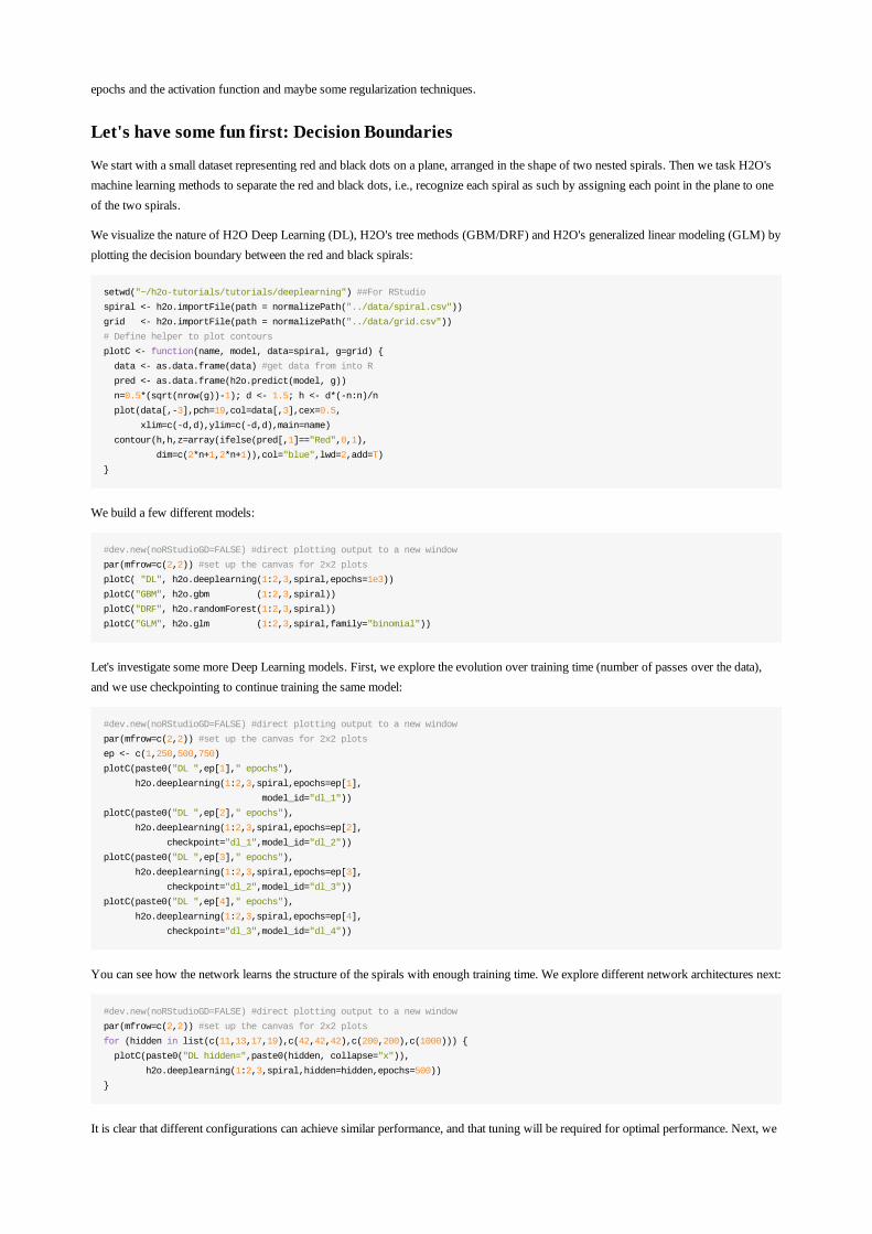
We start with a small dataset representing red and black dots on a plane, arranged in the shape of two nested spirals. Then we task H2O'smachine learning methods to separate the red and black dots, i.e., recognize each spiral as such by assigning each point in the plane to oneof the two spirals.
We visualize the nature of H2O Deep Learning (DL), H2O's tree methods (GBM/DRF) and H2O's generalized linear modeling (GLM) byplotting the decision boundary between the red and black spirals:
setwd("~/h2o-tutorials/tutorials/deeplearning") ##For RStudio
spiral <- h2o.importFile(path = normalizePath("../data/spiral.csv"))
grid <- h2o.importFile(path = normalizePath("../data/grid.csv"))
# Define helper to plot contours
plotC <- function(name, model, data=spiral, g=grid) {
data <- as.data.frame(data) #get data from into R
pred <- as.data.frame(h2o.predict(model, g))
n=0.5*(sqrt(nrow(g))-1); d <- 1.5; h <- d*(-n:n)/n
plot(data[,-3],pch=19,col=data[,3],cex=0.5,
xlim=c(-d,d),ylim=c(-d,d),main=name)
contour(h,h,z=array(ifelse(pred[,1]=="Red",0,1),
dim=c(2*n+1,2*n+1)),col="blue",lwd=2,add=T)
}
We build a few different models:
#dev.new(noRStudioGD=FALSE) #direct plotting output to a new window
par(mfrow=c(2,2)) #set up the canvas for 2x2 plots
plotC( "DL", h2o.deeplearning(1:2,3,spiral,epochs=1e3))
plotC("GBM", h2o.gbm (1:2,3,spiral))
plotC("DRF", h2o.randomForest(1:2,3,spiral))
plotC("GLM", h2o.glm (1:2,3,spiral,family="binomial"))
Let's investigate some more Deep Learning models. First, we explore the evolution over training time (number of passes over the data),and we use checkpointing to continue training the same model:
#dev.new(noRStudioGD=FALSE) #direct plotting output to a new window
par(mfrow=c(2,2)) #set up the canvas for 2x2 plots
ep <- c(1,250,500,750)
plotC(paste0("DL ",ep[1]," epochs"),
h2o.deeplearning(1:2,3,spiral,epochs=ep[1],
model_id="dl_1"))
plotC(paste0("DL ",ep[2]," epochs"),
h2o.deeplearning(1:2,3,spiral,epochs=ep[2],
checkpoint="dl_1",model_id="dl_2"))
plotC(paste0("DL ",ep[3]," epochs"),
h2o.deeplearning(1:2,3,spiral,epochs=ep[3],
checkpoint="dl_2",model_id="dl_3"))
plotC(paste0("DL ",ep[4]," epochs"),
h2o.deeplearning(1:2,3,spiral,epochs=ep[4],
checkpoint="dl_3",model_id="dl_4"))
You can see how the network learns the structure of the spirals with enough training time. We explore different network architectures next:
#dev.new(noRStudioGD=FALSE) #direct plotting output to a new window
par(mfrow=c(2,2)) #set up the canvas for 2x2 plots
for (hidden in list(c(11,13,17,19),c(42,42,42),c(200,200),c(1000))) {
plotC(paste0("DL hidden=",paste0(hidden, collapse="x")),
h2o.deeplearning(1:2,3,spiral,hidden=hidden,epochs=500))
}
It is clear that different configurations can achieve similar performance, and that tuning will be required for optimal performance. Next, we
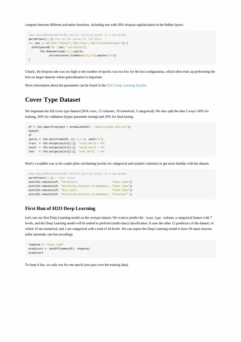
compare between different activation functions, including one with 50% dropout regularization in the hidden layers:
#dev.new(noRStudioGD=FALSE) #direct plotting output to a new window
par(mfrow=c(2,2)) #set up the canvas for 2x2 plots
for (act in c("Tanh","Maxout","Rectifier","RectifierWithDropout")) {
plotC(paste0("DL ",act," activation"),
h2o.deeplearning(1:2,3,spiral,
activation=act,hidden=c(100,100),epochs=1000))
}
Clearly, the dropout rate was too high or the number of epochs was too low for the last configuration, which often ends up performing thebest on larger datasets where generalization is important.
More information about the parameters can be found in the H2O Deep Learning booklet.
Cover Type DatasetWe important the full cover type dataset (581k rows, 13 columns, 10 numerical, 3 categorical). We also split the data 3 ways: 60% fortraining, 20% for validation (hyper parameter tuning) and 20% for final testing.
df <- h2o.importFile(path = normalizePath("../data/covtype.full.csv"))
dim(df)
df
splits <- h2o.splitFrame(df, c(0.6,0.2), seed=1234)
train <- h2o.assign(splits[[1]], "train.hex") # 60%
valid <- h2o.assign(splits[[2]], "valid.hex") # 20%
test <- h2o.assign(splits[[3]], "test.hex") # 20%
Here's a scalable way to do scatter plots via binning (works for categorical and numeric columns) to get more familiar with the dataset.
#dev.new(noRStudioGD=FALSE) #direct plotting output to a new window
par(mfrow=c(1,1)) # reset canvas
plot(h2o.tabulate(df, "Elevation", "Cover_Type"))
plot(h2o.tabulate(df, "Horizontal_Distance_To_Roadways", "Cover_Type"))
plot(h2o.tabulate(df, "Soil_Type", "Cover_Type"))
plot(h2o.tabulate(df, "Horizontal_Distance_To_Roadways", "Elevation" ))
First Run of H2O Deep Learning
Let's run our first Deep Learning model on the covtype dataset. We want to predict the Cover_Type column, a categorical feature with 7levels, and the Deep Learning model will be tasked to perform (multi-class) classification. It uses the other 12 predictors of the dataset, ofwhich 10 are numerical, and 2 are categorical with a total of 44 levels. We can expect the Deep Learning model to have 56 input neurons(after automatic one-hot encoding).
response <- "Cover_Type"
predictors <- setdiff(names(df), response)
predictors
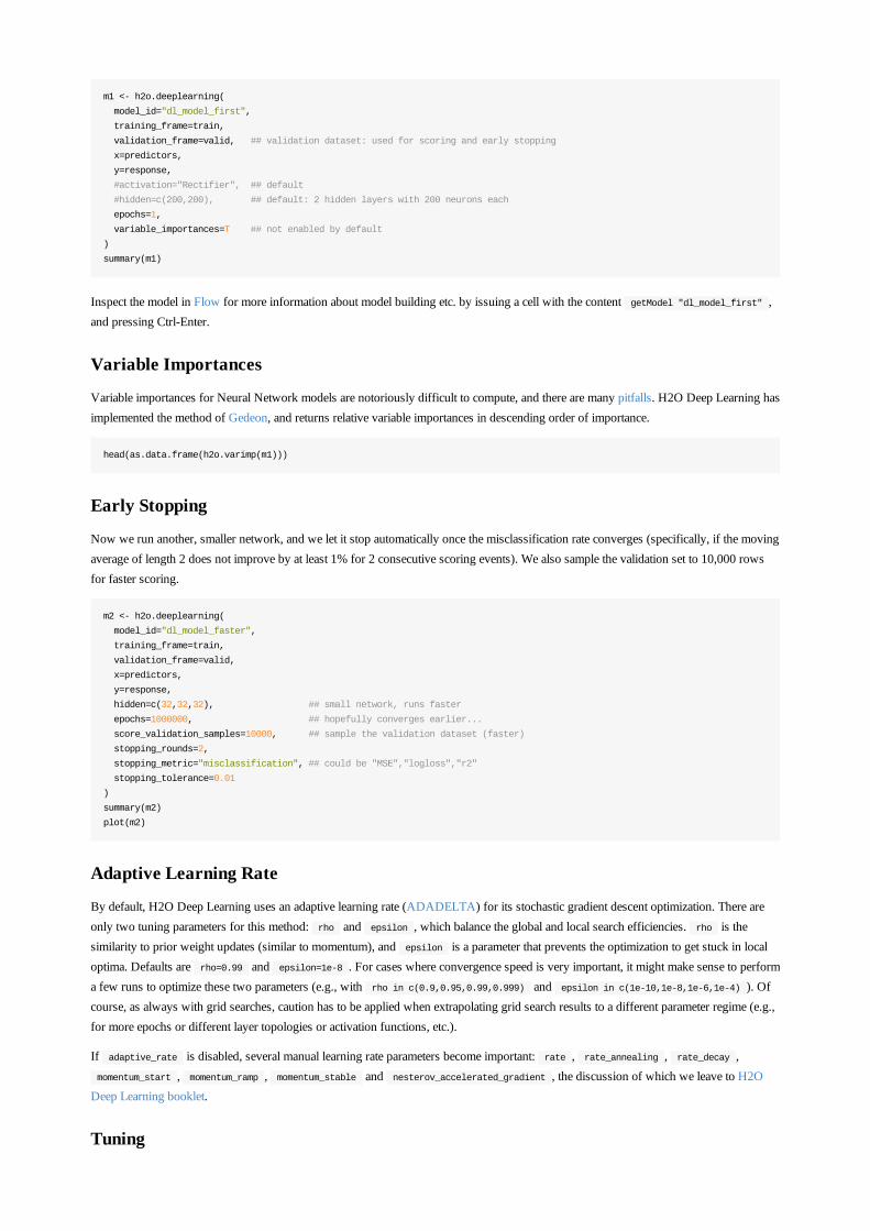
To keep it fast, we only run for one epoch (one pass over the training data).
m1 <- h2o.deeplearning(
model_id="dl_model_first",
training_frame=train,
validation_frame=valid, ## validation dataset: used for scoring and early stopping
x=predictors,
y=response,
#activation="Rectifier", ## default
#hidden=c(200,200), ## default: 2 hidden layers with 200 neurons each
epochs=1,
variable_importances=T ## not enabled by default
)
summary(m1)
Inspect the model in Flow for more information about model building etc. by issuing a cell with the content getModel "dl_model_first" ,and pressing Ctrl-Enter.
Variable Importances
Variable importances for Neural Network models are notoriously difficult to compute, and there are many pitfalls. H2O Deep Learning hasimplemented the method of Gedeon, and returns relative variable importances in descending order of importance.
head(as.data.frame(h2o.varimp(m1)))
Early Stopping
Now we run another, smaller network, and we let it stop automatically once the misclassification rate converges (specifically, if the movingaverage of length 2 does not improve by at least 1% for 2 consecutive scoring events). We also sample the validation set to 10,000 rowsfor faster scoring.
m2 <- h2o.deeplearning(
model_id="dl_model_faster",
training_frame=train,
validation_frame=valid,
x=predictors,
y=response,
hidden=c(32,32,32), ## small network, runs faster
epochs=1000000, ## hopefully converges earlier...
score_validation_samples=10000, ## sample the validation dataset (faster)
stopping_rounds=2,
stopping_metric="misclassification", ## could be "MSE","logloss","r2"
stopping_tolerance=0.01
)
summary(m2)
plot(m2)
Adaptive Learning Rate
By default, H2O Deep Learning uses an adaptive learning rate (ADADELTA) for its stochastic gradient descent optimization. There areonly two tuning parameters for this method: rho and epsilon , which balance the global and local search efficiencies. rho is thesimilarity to prior weight updates (similar to momentum), and epsilon is a parameter that prevents the optimization to get stuck in localoptima. Defaults are rho=0.99 and epsilon=1e-8 . For cases where convergence speed is very important, it might make sense to performa few runs to optimize these two parameters (e.g., with rho in c(0.9,0.95,0.99,0.999) and epsilon in c(1e-10,1e-8,1e-6,1e-4) ). Ofcourse, as always with grid searches, caution has to be applied when extrapolating grid search results to a different parameter regime (e.g.,for more epochs or different layer topologies or activation functions, etc.).
If adaptive_rate is disabled, several manual learning rate parameters become important: rate , rate_annealing , rate_decay , momentum_start , momentum_ramp , momentum_stable and nesterov_accelerated_gradient , the discussion of which we leave to H2ODeep Learning booklet.
Tuning
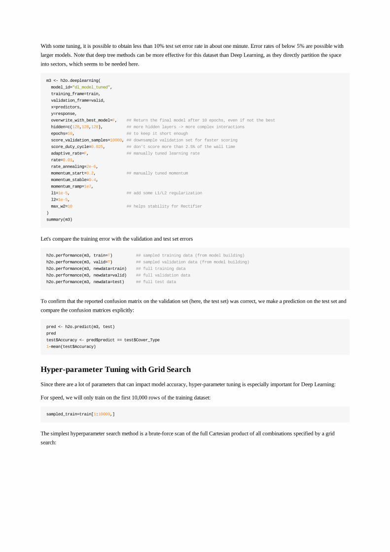
With some tuning, it is possible to obtain less than 10% test set error rate in about one minute. Error rates of below 5% are possible withlarger models. Note that deep tree methods can be more effective for this dataset than Deep Learning, as they directly partition the spaceinto sectors, which seems to be needed here.
m3 <- h2o.deeplearning(
model_id="dl_model_tuned",
training_frame=train,
validation_frame=valid,
x=predictors,
y=response,
overwrite_with_best_model=F, ## Return the final model after 10 epochs, even if not the best
hidden=c(128,128,128), ## more hidden layers -> more complex interactions
epochs=10, ## to keep it short enough
score_validation_samples=10000, ## downsample validation set for faster scoring
score_duty_cycle=0.025, ## don't score more than 2.5% of the wall time
adaptive_rate=F, ## manually tuned learning rate
rate=0.01,
rate_annealing=2e-6,
momentum_start=0.2, ## manually tuned momentum
momentum_stable=0.4,
momentum_ramp=1e7,
l1=1e-5, ## add some L1/L2 regularization
l2=1e-5,
max_w2=10 ## helps stability for Rectifier
)
summary(m3)
Let's compare the training error with the validation and test set errors
h2o.performance(m3, train=T) ## sampled training data (from model building)
h2o.performance(m3, valid=T) ## sampled validation data (from model building)
h2o.performance(m3, newdata=train) ## full training data
h2o.performance(m3, newdata=valid) ## full validation data
h2o.performance(m3, newdata=test) ## full test data
To confirm that the reported confusion matrix on the validation set (here, the test set) was correct, we make a prediction on the test set andcompare the confusion matrices explicitly:
pred <- h2o.predict(m3, test)
pred
test$Accuracy <- pred$predict == test$Cover_Type
1-mean(test$Accuracy)
Hyper-parameter Tuning with Grid Search
Since there are a lot of parameters that can impact model accuracy, hyper-parameter tuning is especially important for Deep Learning:
For speed, we will only train on the first 10,000 rows of the training dataset:
sampled_train=train[1:10000,]
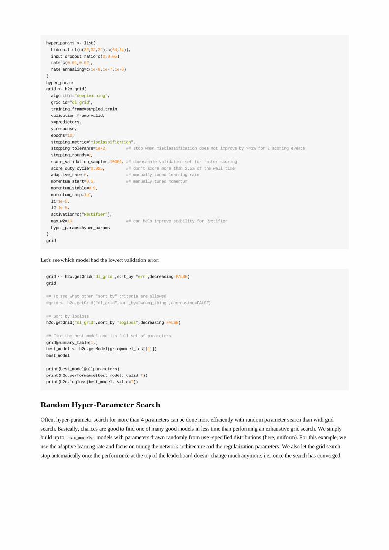
The simplest hyperparameter search method is a brute-force scan of the full Cartesian product of all combinations specified by a gridsearch:
hyper_params <- list(
hidden=list(c(32,32,32),c(64,64)),
input_dropout_ratio=c(0,0.05),
rate=c(0.01,0.02),
rate_annealing=c(1e-8,1e-7,1e-6)
)
hyper_params
grid <- h2o.grid(
algorithm="deeplearning",
grid_id="dl_grid",
training_frame=sampled_train,
validation_frame=valid,
x=predictors,
y=response,
epochs=10,
stopping_metric="misclassification",
stopping_tolerance=1e-2, ## stop when misclassification does not improve by >=1% for 2 scoring events
stopping_rounds=2,
score_validation_samples=10000, ## downsample validation set for faster scoring
score_duty_cycle=0.025, ## don't score more than 2.5% of the wall time
adaptive_rate=F, ## manually tuned learning rate
momentum_start=0.5, ## manually tuned momentum
momentum_stable=0.9,
momentum_ramp=1e7,
l1=1e-5,
l2=1e-5,
activation=c("Rectifier"),
max_w2=10, ## can help improve stability for Rectifier
hyper_params=hyper_params
)
grid
Let's see which model had the lowest validation error:
grid <- h2o.getGrid("dl_grid",sort_by="err",decreasing=FALSE)
grid
## To see what other "sort_by" criteria are allowed
#grid <- h2o.getGrid("dl_grid",sort_by="wrong_thing",decreasing=FALSE)
## Sort by logloss
h2o.getGrid("dl_grid",sort_by="logloss",decreasing=FALSE)
## Find the best model and its full set of parameters
grid@summary_table[1,]
best_model <- h2o.getModel(grid@model_ids[[1]])
best_model
print(best_model@allparameters)
print(h2o.performance(best_model, valid=T))
print(h2o.logloss(best_model, valid=T))
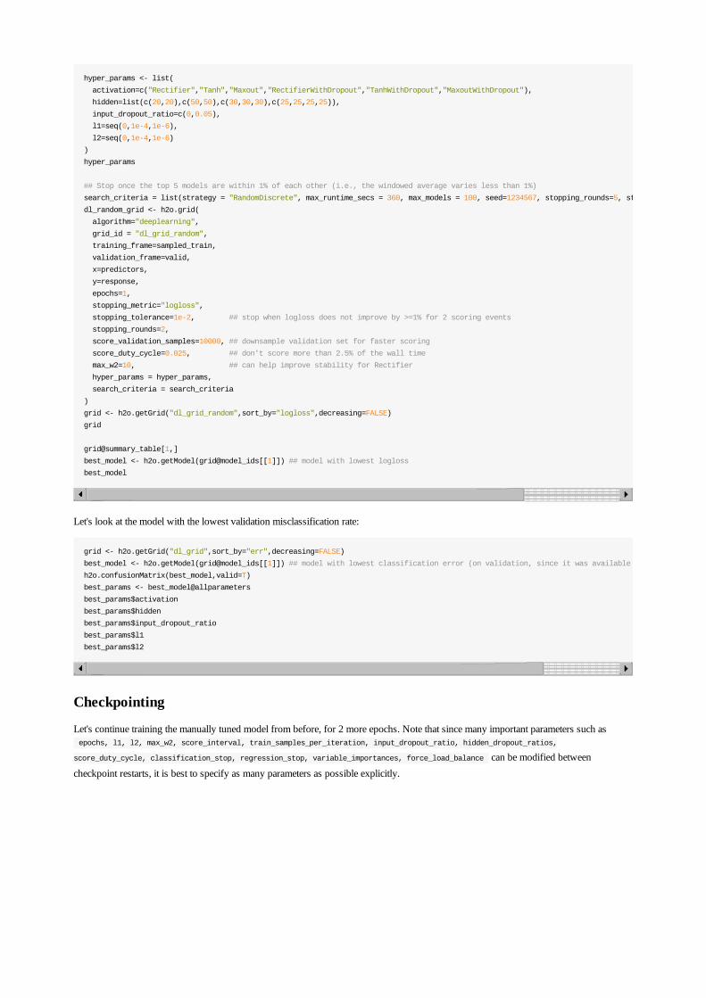
Random Hyper-Parameter Search
Often, hyper-parameter search for more than 4 parameters can be done more efficiently with random parameter search than with gridsearch. Basically, chances are good to find one of many good models in less time than performing an exhaustive grid search. We simplybuild up to max_models models with parameters drawn randomly from user-specified distributions (here, uniform). For this example, weuse the adaptive learning rate and focus on tuning the network architecture and the regularization parameters. We also let the grid searchstop automatically once the performance at the top of the leaderboard doesn't change much anymore, i.e., once the search has converged.
hyper_params <- list(
activation=c("Rectifier","Tanh","Maxout","RectifierWithDropout","TanhWithDropout","MaxoutWithDropout"),
hidden=list(c(20,20),c(50,50),c(30,30,30),c(25,25,25,25)),
input_dropout_ratio=c(0,0.05),
l1=seq(0,1e-4,1e-6),
l2=seq(0,1e-4,1e-6)
)
hyper_params
## Stop once the top 5 models are within 1% of each other (i.e., the windowed average varies less than 1%)
search_criteria = list(strategy = "RandomDiscrete", max_runtime_secs = 360, max_models = 100, seed=1234567, stopping_rounds=5, stopping_tolerance=
dl_random_grid <- h2o.grid(
algorithm="deeplearning",
grid_id = "dl_grid_random",
training_frame=sampled_train,
validation_frame=valid,
x=predictors,
y=response,
epochs=1,
stopping_metric="logloss",
stopping_tolerance=1e-2, ## stop when logloss does not improve by >=1% for 2 scoring events
stopping_rounds=2,
score_validation_samples=10000, ## downsample validation set for faster scoring
score_duty_cycle=0.025, ## don't score more than 2.5% of the wall time
max_w2=10, ## can help improve stability for Rectifier
hyper_params = hyper_params,
search_criteria = search_criteria
)
grid <- h2o.getGrid("dl_grid_random",sort_by="logloss",decreasing=FALSE)
grid
grid@summary_table[1,]
best_model <- h2o.getModel(grid@model_ids[[1]]) ## model with lowest logloss
best_model
Let's look at the model with the lowest validation misclassification rate:
grid <- h2o.getGrid("dl_grid",sort_by="err",decreasing=FALSE)
best_model <- h2o.getModel(grid@model_ids[[1]]) ## model with lowest classification error (on validation, since it was available during training)
h2o.confusionMatrix(best_model,valid=T)
best_params <- best_model@allparameters
best_params$activation
best_params$hidden
best_params$input_dropout_ratio
best_params$l1
best_params$l2
Checkpointing
Let's continue training the manually tuned model from before, for 2 more epochs. Note that since many important parameters such as epochs, l1, l2, max_w2, score_interval, train_samples_per_iteration, input_dropout_ratio, hidden_dropout_ratios,
score_duty_cycle, classification_stop, regression_stop, variable_importances, force_load_balance can be modified betweencheckpoint restarts, it is best to specify as many parameters as possible explicitly.
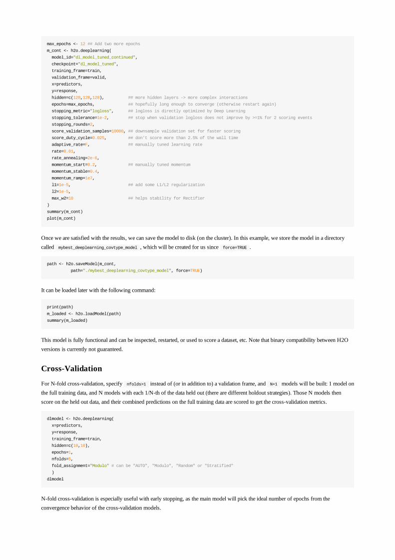
max_epochs <- 12 ## Add two more epochs
m_cont <- h2o.deeplearning(
model_id="dl_model_tuned_continued",
checkpoint="dl_model_tuned",
training_frame=train,
validation_frame=valid,
x=predictors,
y=response,
hidden=c(128,128,128), ## more hidden layers -> more complex interactions
epochs=max_epochs, ## hopefully long enough to converge (otherwise restart again)
stopping_metric="logloss", ## logloss is directly optimized by Deep Learning
stopping_tolerance=1e-2, ## stop when validation logloss does not improve by >=1% for 2 scoring events
stopping_rounds=2,
score_validation_samples=10000, ## downsample validation set for faster scoring
score_duty_cycle=0.025, ## don't score more than 2.5% of the wall time
adaptive_rate=F, ## manually tuned learning rate
rate=0.01,
rate_annealing=2e-6,
momentum_start=0.2, ## manually tuned momentum
momentum_stable=0.4,
momentum_ramp=1e7,
l1=1e-5, ## add some L1/L2 regularization
l2=1e-5,
max_w2=10 ## helps stability for Rectifier
)
summary(m_cont)
plot(m_cont)
Once we are satisfied with the results, we can save the model to disk (on the cluster). In this example, we store the model in a directorycalled mybest_deeplearning_covtype_model , which will be created for us since force=TRUE .
path <- h2o.saveModel(m_cont,
path="./mybest_deeplearning_covtype_model", force=TRUE)
It can be loaded later with the following command:
print(path)
m_loaded <- h2o.loadModel(path)
summary(m_loaded)
This model is fully functional and can be inspected, restarted, or used to score a dataset, etc. Note that binary compatibility between H2Oversions is currently not guaranteed.
Cross-Validation
For N-fold cross-validation, specify nfolds>1 instead of (or in addition to) a validation frame, and N+1 models will be built: 1 model onthe full training data, and N models with each 1/N-th of the data held out (there are different holdout strategies). Those N models thenscore on the held out data, and their combined predictions on the full training data are scored to get the cross-validation metrics.
dlmodel <- h2o.deeplearning(
x=predictors,
y=response,
training_frame=train,
hidden=c(10,10),
epochs=1,
nfolds=5,
fold_assignment="Modulo" # can be "AUTO", "Modulo", "Random" or "Stratified"
)
dlmodel
N-fold cross-validation is especially useful with early stopping, as the main model will pick the ideal number of epochs from theconvergence behavior of the cross-validation models.
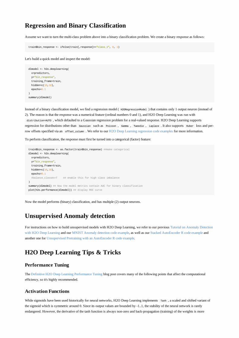
Regression and Binary ClassificationAssume we want to turn the multi-class problem above into a binary classification problem. We create a binary response as follows:
train$bin_response <- ifelse(train[,response]=="class_1", 0, 1)
Let's build a quick model and inspect the model:
dlmodel <- h2o.deeplearning(
x=predictors,
y="bin_response",
training_frame=train,
hidden=c(10,10),
epochs=0.1
)
summary(dlmodel)
Instead of a binary classification model, we find a regression model ( H2ORegressionModel ) that contains only 1 output neuron (instead of2). The reason is that the response was a numerical feature (ordinal numbers 0 and 1), and H2O Deep Learning was run with distribution=AUTO , which defaulted to a Gaussian regression problem for a real-valued response. H2O Deep Learning supportsregression for distributions other than Gaussian such as Poisson , Gamma , Tweedie , Laplace . It also supports Huber loss and per-row offsets specified via an offset_column . We refer to our H2O Deep Learning regression code examples for more information.
To perform classification, the response must first be turned into a categorical (factor) feature:
train$bin_response <- as.factor(train$bin_response) ##make categorical
dlmodel <- h2o.deeplearning(
x=predictors,
y="bin_response",
training_frame=train,
hidden=c(10,10),
epochs=0.1
#balance_classes=T ## enable this for high class imbalance
)
summary(dlmodel) ## Now the model metrics contain AUC for binary classification
plot(h2o.performance(dlmodel)) ## display ROC curve
Now the model performs (binary) classification, and has multiple (2) output neurons.
Unsupervised Anomaly detectionFor instructions on how to build unsupervised models with H2O Deep Learning, we refer to our previous Tutorial on Anomaly Detectionwith H2O Deep Learning and our MNIST Anomaly detection code example, as well as our Stacked AutoEncoder R code example andanother one for Unsupervised Pretraining with an AutoEncoder R code example.
H2O Deep Learning Tips & Tricks
Performance Tuning
The Definitive H2O Deep Learning Performance Tuning blog post covers many of the following points that affect the computationalefficiency, so it's highly recommended.
Activation Functions
While sigmoids have been used historically for neural networks, H2O Deep Learning implements Tanh , a scaled and shifted variant ofthe sigmoid which is symmetric around 0. Since its output values are bounded by -1..1, the stability of the neural network is rarelyendangered. However, the derivative of the tanh function is always non-zero and back-propagation (training) of the weights is more
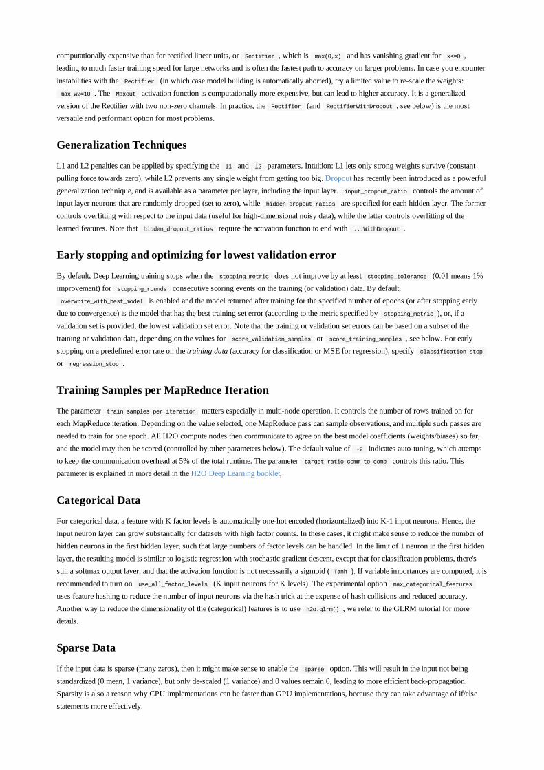
computationally expensive than for rectified linear units, or Rectifier , which is max(0,x) and has vanishing gradient for x<=0 ,leading to much faster training speed for large networks and is often the fastest path to accuracy on larger problems. In case you encounterinstabilities with the Rectifier (in which case model building is automatically aborted), try a limited value to re-scale the weights: max_w2=10 . The Maxout activation function is computationally more expensive, but can lead to higher accuracy. It is a generalizedversion of the Rectifier with two non-zero channels. In practice, the Rectifier (and RectifierWithDropout , see below) is the mostversatile and performant option for most problems.
Generalization Techniques
L1 and L2 penalties can be applied by specifying the l1 and l2 parameters. Intuition: L1 lets only strong weights survive (constantpulling force towards zero), while L2 prevents any single weight from getting too big. Dropout has recently been introduced as a powerfulgeneralization technique, and is available as a parameter per layer, including the input layer. input_dropout_ratio controls the amount ofinput layer neurons that are randomly dropped (set to zero), while hidden_dropout_ratios are specified for each hidden layer. The formercontrols overfitting with respect to the input data (useful for high-dimensional noisy data), while the latter controls overfitting of thelearned features. Note that hidden_dropout_ratios require the activation function to end with ...WithDropout .
Early stopping and optimizing for lowest validation error
By default, Deep Learning training stops when the stopping_metric does not improve by at least stopping_tolerance (0.01 means 1%improvement) for stopping_rounds consecutive scoring events on the training (or validation) data. By default, overwrite_with_best_model is enabled and the model returned after training for the specified number of epochs (or after stopping earlydue to convergence) is the model that has the best training set error (according to the metric specified by stopping_metric ), or, if avalidation set is provided, the lowest validation set error. Note that the training or validation set errors can be based on a subset of thetraining or validation data, depending on the values for score_validation_samples or score_training_samples , see below. For earlystopping on a predefined error rate on the training data (accuracy for classification or MSE for regression), specify classification_stop or regression_stop .
Training Samples per MapReduce Iteration
The parameter train_samples_per_iteration matters especially in multi-node operation. It controls the number of rows trained on foreach MapReduce iteration. Depending on the value selected, one MapReduce pass can sample observations, and multiple such passes areneeded to train for one epoch. All H2O compute nodes then communicate to agree on the best model coefficients (weights/biases) so far,and the model may then be scored (controlled by other parameters below). The default value of -2 indicates auto-tuning, which attempsto keep the communication overhead at 5% of the total runtime. The parameter target_ratio_comm_to_comp controls this ratio. Thisparameter is explained in more detail in the H2O Deep Learning booklet,
Categorical Data
For categorical data, a feature with K factor levels is automatically one-hot encoded (horizontalized) into K-1 input neurons. Hence, theinput neuron layer can grow substantially for datasets with high factor counts. In these cases, it might make sense to reduce the number ofhidden neurons in the first hidden layer, such that large numbers of factor levels can be handled. In the limit of 1 neuron in the first hiddenlayer, the resulting model is similar to logistic regression with stochastic gradient descent, except that for classification problems, there'sstill a softmax output layer, and that the activation function is not necessarily a sigmoid ( Tanh ). If variable importances are computed, it isrecommended to turn on use_all_factor_levels (K input neurons for K levels). The experimental option max_categorical_features uses feature hashing to reduce the number of input neurons via the hash trick at the expense of hash collisions and reduced accuracy.Another way to reduce the dimensionality of the (categorical) features is to use h2o.glrm() , we refer to the GLRM tutorial for moredetails.
Sparse Data
If the input data is sparse (many zeros), then it might make sense to enable the sparse option. This will result in the input not beingstandardized (0 mean, 1 variance), but only de-scaled (1 variance) and 0 values remain 0, leading to more efficient back-propagation.Sparsity is also a reason why CPU implementations can be faster than GPU implementations, because they can take advantage of if/elsestatements more effectively.
Missing Values
H2O Deep Learning automatically does mean imputation for missing values during training (leaving the input layer activation at 0 afterstandardizing the values). For testing, missing test set values are also treated the same way by default. See the h2o.impute function to doyour own mean imputation.
Loss functions, Distributions, Offsets, Observation Weights
H2O Deep Learning supports advanced statistical features such as multiple loss functions, non-Gaussian distributions, per-row offsets andobservation weights. In addition to Gaussian distributions and Squared loss, H2O Deep Learning supports Poisson , Gamma , Tweedie and Laplace distributions. It also supports Absolute and Huber loss and per-row offsets specified via an offset_column .Observation weights are supported via a user-specified weights_column .
We refer to our H2O Deep Learning R test code examples for more information.
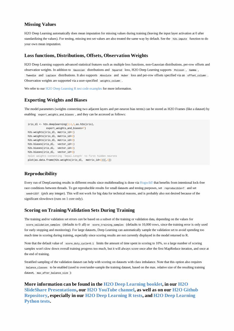
Exporting Weights and Biases
The model parameters (weights connecting two adjacent layers and per-neuron bias terms) can be stored as H2O Frames (like a dataset) byenabling export_weights_and_biases , and they can be accessed as follows:
iris_dl <- h2o.deeplearning(1:4,5,as.h2o(iris),
export_weights_and_biases=T)
h2o.weights(iris_dl, matrix_id=1)
h2o.weights(iris_dl, matrix_id=2)
h2o.weights(iris_dl, matrix_id=3)
h2o.biases(iris_dl, vector_id=1)
h2o.biases(iris_dl, vector_id=2)
h2o.biases(iris_dl, vector_id=3)
#plot weights connecting `Sepal.Length` to first hidden neurons
plot(as.data.frame(h2o.weights(iris_dl, matrix_id=1))[,1])
Reproducibility
Every run of DeepLearning results in different results since multithreading is done via Hogwild! that benefits from intentional lock-freerace conditions between threads. To get reproducible results for small datasets and testing purposes, set reproducible=T and set seed=1337 (pick any integer). This will not work for big data for technical reasons, and is probably also not desired because of thesignificant slowdown (runs on 1 core only).
Scoring on Training/Validation Sets During Training
The training and/or validation set errors can be based on a subset of the training or validation data, depending on the values for score_validation_samples (defaults to 0: all) or score_training_samples (defaults to 10,000 rows, since the training error is only usedfor early stopping and monitoring). For large datasets, Deep Learning can automatically sample the validation set to avoid spending toomuch time in scoring during training, especially since scoring results are not currently displayed in the model returned to R.
Note that the default value of score_duty_cycle=0.1 limits the amount of time spent in scoring to 10%, so a large number of scoringsamples won't slow down overall training progress too much, but it will always score once after the first MapReduce iteration, and once atthe end of training.
Stratified sampling of the validation dataset can help with scoring on datasets with class imbalance. Note that this option also requires balance_classes to be enabled (used to over/under-sample the training dataset, based on the max. relative size of the resulting trainingdataset, max_after_balance_size ):
More information can be found in the H2O Deep Learning booklet, in our H2OSlideShare Presentations, our H2O YouTube channel, as well as on our H2O GithubRepository, especially in our H2O Deep Learning R tests, and H2O Deep LearningPython tests.

All done, shutdown H2O
h2o.shutdown(prompt=FALSE)

GBM and Random Forest in H2O
SlidesPDF
CodeThe source code for this example is here: R script
IntroductionInstallation and Startup
Cover Type DatasetMultinomial ModelBinomial Model
Adding extra featuresMultinomial Model Revisited
IntroductionThis tutorial shows how a H2O GLM model can be used to do binary and multi-class classification. This tutorial covers usage of H2Ofrom R. A python version of this tutorial will be available as well in a separate document. This file is available in plain R, R markdown andregular markdown formats, and the plots are available as PDF files. All documents are available on Github.
If run from plain R, execute R in the directory of this script. If run from RStudio, be sure to setwd() to the location of this script. h2o.init() starts H2O in R's current working directory. h2o.importFile() looks for files from the perspective of where H2O was started.
More examples and explanations can be found in our H2O GLM booklet and on our H2O Github Repository.
H2O R Package
Load the H2O R package:
## R installation instructions are at http://h2o.ai/download
library(h2o)
Start H2O
Start up a 1-node H2O server on your local machine, and allow it to use all CPU cores and up to 2GB of memory:
h2o.init(nthreads=-1, max_mem_size="2G")
h2o.removeAll() ## clean slate - just in case the cluster was already running
Cover Type DataPredicting forest cover type from cartographic variables only (no remotely sensed data). Let's import the dataset:
D = h2o.importFile(path = normalizePath("../data/covtype.full.csv"))
h2o.summary(D)
We have 11 numeric and two categorical features. Response is "Cover_Type" and has 7 classes. Let's split the data intoTrain/Test/Validation with train having 70% and Test and Validation 15% each:
data = h2o.splitFrame(D,ratios=c(.7,.15),destination_frames = c("train","test","valid"))
names(data)
Multinomial ModelWe imported our data, so let's run GLM. As we mentioned previously, Cover_Type is the response and we use all other columns aspredictors. We have multi-class problem so we pick family=multinomial. L-BFGS solver tends to be faster on multinomial problems, sowe pick L-BFGS for our first try. The rest can use the default settings.
m1 = h2o.glm(training_frame = data$Train, validation_frame = data$Valid, x = x, y = y,family='multinomial',solver='L_BFGS')
h2o.confusionMatrix(m1, valid=TRUE)
The model predicts only the majority class so it's not useful at all! Maybe we regularized it too much, let's try again without regularization:
m2 = h2o.glm(training_frame = data$Train, validation_frame = data$Valid, x = x, y = y,family='multinomial',solver='L_BFGS', lambda = 0)
h2o.confusionMatrix(m2, valid=FALSE) # get confusion matrix in the training data
h2o.confusionMatrix(m2, valid=TRUE) # get confusion matrix in the validation data
No overfitting (as train and test performance are the same), regularization is not needed in this case.
This model is actually useful. It got 28% classification error, down from 51% obtained by predicting majority class only.
Binomial ModelSince multinomial models are difficult and time consuming, let's try a simpler binary classification. We'll take a subset of the data with only class_1 and class_2 (the two majority classes) and build a binomial model deciding between them.
D_binomial = D[D$Cover_Type %in% c("class_1","class_2"),]
h2o.setLevels(D_binomial$Cover_Type,c("class_1","class_2"))
# split to train/test/validation again
data_binomial = h2o.splitFrame(D_binomial,ratios=c(.7,.15),destination_frames = c("train_b","test_b","valid_b"))
names(data_binomial)
We can run a binomial model now:
m_binomial = h2o.glm(training_frame = data_binomial$Train, validation_frame = data_binomial$Valid, x = x, y = y, family='binomial',lambda=0)
h2o.confusionMatrix(m_binomial, valid = TRUE)
h2o.confusionMatrix(m_binomial, valid = TRUE)
The output for a binomial problem is slightly different from multinomial. The confusion matrix now has a threshold attached to it.
The model produces probability of class_1 and class_2 similarly to multinomial example earlier. However, this time we only have twoclasses and we can tune the classification to our needs.
The classification errors in binomial cases have a particular meaning: we call them false-positive and false negative. In reality, each canhave a different cost associated with it, so we want to tune our classifier accordingly.
The common way to evaluate a binary classifier performance is to look at its ROC curve. The ROC curve plots the true positive rate versusfalse positive rate. We can plot it from the H2O model output:
fpr = m_binomial@model$training_metrics@metrics$thresholds_and_metric_scores$fpr
tpr = m_binomial@model$training_metrics@metrics$thresholds_and_metric_scores$tpr
fpr_val = m_binomial@model$validation_metrics@metrics$thresholds_and_metric_scores$fpr
tpr_val = m_binomial@model$validation_metrics@metrics$thresholds_and_metric_scores$tpr
plot(fpr,tpr, type='l')
title('AUC')
lines(fpr_val,tpr_val,type='l',col='red')
legend("bottomright",c("Train", "Validation"),col=c("black","red"),lty=c(1,1),lwd=c(3,3))
The area under the ROC curve (AUC) is a common "good fit" metric for binary classifiers. For this example, the results were:
h2o.auc(m_binomial,valid=FALSE) # on train
h2o.auc(m_binomial,valid=TRUE) # on test
The default confusion matrix is computed at thresholds that optimize the F1 score. We can choose different thresholds - the H2O outputshows optimal thresholds for some common metrics.
m_binomial@model$training_metrics@metrics$max_criteria_and_metric_scores
The model we just built gets 23% classification error at the F1-optimizing threshold, so there is still room for improvement. Let's add somefeatures:
There are 11 numerical predictors in the dataset, we will cut them into intervals and add a categorical variable for eachWe can add interaction terms capturing interactions between categorical variables
Let's make a convenience function to cut the column into intervals working on all three of our datasets (Train/Validation/Test). We'll use h2o.hist to determine interval boundaries (but there are many more ways to do that!) on the Train set.We'll take only the bins with non-trivial support:
cut_column <- function(data,="" col)="" {="" #="" need="" lower="" upper="" bound="" due="" to="" h2o.cut="" behavior="" (points="" <="" the="" first="" break="" or=""> the last break are replaced with missing value)
min_val = min(data$Train[,col])-1
max_val = max(data$Train[,col])+1
x = h2o.hist(data$Train[, col])
# use only the breaks with enough support
breaks = x$breaks[which(x$counts > 1000)]
# assign level names
lvls = c("min",paste("i_",breaks[2:length(breaks)-1],sep=""),"max")
col_cut
Now let's make a convenience function generating interaction terms on all three of our datasets. We'll use h2o.interaction :
interactions
Finally, let's wrap addition of the features into a separate function call, as we will use it again later. We'll add intervals for each numericcolumn and interactions between each pair of binary columns.
# add features to our cover type example
# let's cut all the numerical columns into intervals and add interactions between categorical terms
add_features
Now we generate new features and add them to the dataset. We'll also need to generate column names again, as we added more columns:
# Add Features
data_binomial_ext
Let's build the model! We should add some regularization this time because we added correlated variables, so let's try the default:
m_binomial_1_ext = try(h2o.glm(training_frame = data_binomial_ext$Train, validation_frame = data_binomial_ext$Valid, x = x, y = y, family='binomial'))
Oops, doesn't run - well, we know have more features than the default method can solve with 2GB of RAM. Let's try L-BFGS instead.
m_binomial_1_ext = h2o.glm(training_frame = data_binomial_ext$Train, validation_frame = data_binomial_ext$Valid, x = x, y = y, family='binomial', solver='L_BFGS')
h2o.confusionMatrix(m_binomial_1_ext)
h2o.auc(m_binomial_1_ext,valid=TRUE)
Not much better, maybe too much regularization? Let's pick a smaller lambda and try again.
m_binomial_2_ext = h2o.glm(training_frame = data_binomial_ext$Train, validation_frame = data_binomial_ext$Valid, x = x, y = y, family='binomial', solver='L_BFGS', lambda=1e-4)
h2o.confusionMatrix(m_binomial_2_ext, valid=TRUE)
h2o.auc(m_binomial_2_ext,valid=TRUE)

Way better, we got an AUC of .91 and classification error of 0.180838. We picked our regularization strength arbitrarily. Also, we usedonly the l2 penalty but we added lot of extra features, some of which may be useless. Maybe we can do better with an l1 penalty. So nowwe want to run a lambda search to find optimal penalty strength and we want to have a non-zero l1 penalty to get sparse solution. We'll usethe IRLSM solver this time as it does much better with lambda search and l1 penalty. Recall we were not able to use it before. We can useit now as we are running a lambda search that will filter out a large portion of the inactive (coefficient==0) predictors.
m_binomial_3_ext = h2o.glm(training_frame = data_binomial_ext$Train, validation_frame = data_binomial_ext$Valid, x = x, y = y, family='binomial', lambda_search=TRUE)
h2o.confusionMatrix(m_binomial_3_ext, valid=TRUE)
h2o.auc(m_binomial_3_ext,valid=TRUE)
Better yet, we have 17% error and we used only 3000 out of 7000 features. Ok, our new features improved the binomial modelsignificantly, so let's revisit our former multinomial model and see if they make a difference there (they should!):
# Multinomial Model 2
# let's revisit the multinomial case with our new features
data_ext
Improved considerably, 21% instead of 28%.
Generalized Low Rank ModelsOverviewWhat is a Low Rank Model?Why use Low Rank Models?
MemorySpeedFeature EngineeringMissing Data Imputation
Example 1: Visualizing Walking StancesBasic Model BuildingPlotting Archetypal FeaturesImputing Missing Values
Example 2: Compressing Zip CodesCondensing Categorical DataRuntime and Accuracy Comparison
References
OverviewThis tutorial introduces the Generalized Low Rank Model (GLRM) [1], a new machine learning approach for reconstructing missingvalues and identifying important features in heterogeneous data. It demonstrates how to build a GLRM in H2O and integrate it into a datascience pipeline to make better predictions.
What is a Low Rank Model?Across business and research, analysts seek to understand large collections of data with numeric and categorical values. Many entries inthis table may be noisy or even missing altogether. Low rank models facilitate the understanding of tabular data by producing a condensedvector representation for every row and column in the data set.
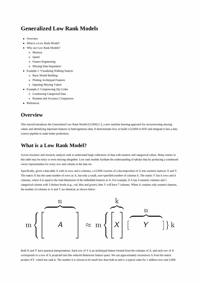
Specifically, given a data table A with m rows and n columns, a GLRM consists of a decomposition of A into numeric matrices X and Y.The matrix X has the same number of rows as A, but only a small, user-specified number of columns k. The matrix Y has k rows and dcolumns, where d is equal to the total dimension of the embedded features in A. For example, if A has 4 numeric columns and 1categorical column with 3 distinct levels (e.g., red, blue and green), then Y will have 7 columns. When A contains only numeric features,the number of columns in A and Y are identical, as shown below.
Both X and Y have practical interpretations. Each row of Y is an archetypal feature formed from the columns of A, and each row of Xcorresponds to a row of A projected into this reduced dimension feature space. We can approximately reconstruct A from the matrixproduct XY, which has rank k. The number k is chosen to be much less than both m and n: a typical value for 1 million rows and 2,000

columns of numeric data is k = 15. The smaller k is, the more compression we gain from our low rank representation.
GLRMs are an extension of well-known matrix factorization methods such as Principal Components Analysis (PCA). While PCA islimited to numeric data, GLRMs can handle mixed numeric, categorical, ordinal and Boolean data with an arbitrary number of missingvalues. It allows the user to apply regularization to X and Y, imposing restrictions like non-negativity appropriate to a particular datascience context. Thus, it is an extremely flexible approach for analyzing and interpreting heterogeneous data sets.
Why use Low Rank Models?Memory: By saving only the X and Y matrices, we can significantly reduce the amount of memory required to store a large data set.A file that is 10 GB can be compressed down to 100 MB. When we need the original data again, we can reconstruct it on the fly fromX and Y with minimal loss in accuracy.Speed: We can use GLRM to compress data with high-dimensional, heterogeneous features into a few numeric columns. This leadsto a huge speed-up in model building and prediction, especially by machine learning algorithms that scale poorly with the size of thefeature space. Below, we will see an example with 10x speed-up and no accuracy loss in deep learning.Feature Engineering: The Y matrix represents the most important combination of features from the training data. These condensedfeatures, called archetypes, can be analyzed, visualized and incorporated into various data science applications.Missing Data Imputation: Reconstructing a data set from X and Y will automatically impute missing values. This imputation isaccomplished by intelligently leveraging the information contained in the known values of each feature, as well as user-providedparameters such as the loss function.
Example 1: Visualizing Walking StancesFor our first example, we will use data on Subject 01's walking stances from an experiment carried out by Hamner and Delp (2013) [2].Each of the 151 rows of the data set contains the (x, y, z) coordinates of major body parts recorded at a specific point in time.
Basic Model Building
Initialize the H2O server and import our walking stance data. We use all available cores on our computer and allocate amaximum of 2 GB of memory to H2O.
library(h2o)
h2o.init(nthreads = -1, max_mem_size = "2G")
gait.hex <- h2o.importFile(path = normalizePath("../data/subject01_walk1.csv"), destination_frame = "gait.hex")
Get a summary of the imported data set.
dim(gait.hex)
summary(gait.hex)
Build a basic GLRM using quadratic loss and no regularization. Since this data set contains only numeric features and nomissing values, this is equivalent to PCA. We skip the first column since it is the time index, set the rank k = 10, and allow thealgorithm to run for a maximum of 1,000 iterations.
gait.glrm <- h2o.glrm(training_frame = gait.hex, cols = 2:ncol(gait.hex), k = 10, loss = "Quadratic",
regularization_x = "None", regularization_y = "None", max_iterations = 1000)
To ensure our algorithm converged, we should always plot the objective function value per iteration after model building iscomplete.
plot(gait.glrm)
Plotting Archetypal Features
The rows of the Y matrix represent the principal stances that Subject 01 took while walking. We can visualize each of the 10stances by plotting the (x, y) coordinate weights of each body part.
gait.y <- gait.glrm@model$archetypes
gait.y.mat <- as.matrix(gait.y)
x_coords <- seq(1, ncol(gait.y), by = 3)
y_coords <- seq(2, ncol(gait.y), by = 3)
feat_nams <- sapply(colnames(gait.y), function(nam) { substr(nam, 1, nchar(nam)-1) })
feat_nams <- as.character(feat_nams[x_coords])
for(k in 1:10) {
plot(gait.y.mat[k,x_coords], gait.y.mat[k,y_coords], xlab = "X-Coordinate Weight", ylab = "Y-Coordinate Weight", main = paste("Feature Weights of Archetype", k), col = "blue", pch = 19, lty = "solid")
text(gait.y.mat[k,x_coords], gait.y.mat[k,y_coords], labels = feat_nams, cex = 0.7, pos = 3)
cat("Press [Enter] to continue")
line <- readline()
}
The rows of the X matrix decompose each bodily position Subject 01 took at a specific time into a combination of the principalstances. Let's plot each principal stance over time to see how they alternate.
gait.x <- h2o.getFrame(gait.glrm@model$representation_name)
time.df <- as.data.frame(gait.hex$Time[1:150])[,1]
gait.x.df <- as.data.frame(gait.x[1:150,])
matplot(time.df, gait.x.df, xlab = "Time", ylab = "Archetypal Projection", main = "Archetypes over Time", type = "l", lty = 1, col = 1:5)
legend("topright", legend = colnames(gait.x.df), col = 1:5, pch = 1)
We can reconstruct our original training data from X and Y.
gait.pred <- predict(gait.glrm, gait.hex)
head(gait.pred)
For comparison, let's plot the original and reconstructed data of a specific feature over time: the x-coordinate of the leftacromium.
lacro.df <- as.data.frame(gait.hex$L.Acromium.X[1:150])
lacro.pred.df <- as.data.frame(gait.pred$reconstr_L.Acromium.X[1:150])
matplot(time.df, cbind(lacro.df, lacro.pred.df), xlab = "Time", ylab = "X-Coordinate of Left Acromium", main = "Position of Left Acromium over Time", type = "l", lty = 1, col = c(1,4))
legend("topright", legend = c("Original", "Reconstructed"), col = c(1,4), pch = 1)
Imputing Missing Values
Suppose that due to a sensor malfunction, our walking stance data has missing values randomly interspersed. We can use GLRM toreconstruct these missing values from the existing data.
Import walking stance data containing 15% missing values and get a summary.
gait.miss <- h2o.importFile(path = normalizePath("../data/subject01_walk1_miss15.csv"), destination_frame = "gait.miss")
dim(gait.miss)
summary(gait.miss)
Count the total number of missing values in the data set.
sum(is.na(gait.miss))
Build a basic GLRM with quadratic loss and no regularization, validating on our original data set that has no missing values.We change the algorithm initialization method, increase the maximum number of iterations to 2,000, and reduce the minimumstep size to 1e-6 to ensure convergence.
gait.glrm2 <- h2o.glrm(training_frame = gait.miss, validation_frame = gait.hex, cols = 2:ncol(gait.miss), k = 10, init = "SVD", svd_method = "GramSVD",
loss = "Quadratic", regularization_x = "None", regularization_y = "None", max_iterations = 2000, min_step_size = 1e-6)
plot(gait.glrm2)
Impute missing values in our training data from X and Y.
gait.pred2 <- predict(gait.glrm2, gait.miss)
head(gait.pred2)
sum(is.na(gait.pred2))
Plot the original and reconstructed values of the x-coordinate of the left acromium. Red x's mark the points where the trainingdata contains a missing value, so we can see how accurate our imputation is.
lacro.pred.df2 <- as.data.frame(gait.pred2$reconstr_L.Acromium.X[1:150])
matplot(time.df, cbind(lacro.df, lacro.pred.df2), xlab = "Time", ylab = "X-Coordinate of Left Acromium", main = "Position of Left Acromium over Time", type = "l", lty = 1, col = c(1,4))
legend("topright", legend = c("Original", "Imputed"), col = c(1,4), pch = 1)
lacro.miss.df <- as.data.frame(gait.miss$L.Acromium.X[1:150])
idx_miss <- which(is.na(lacro.miss.df))
points(time.df[idx_miss], lacro.df[idx_miss,1], col = 2, pch = 4, lty = 2)
Example 2: Compressing Zip CodesFor our second example, we will be using two data sets. The first is compliance actions carried out by the U.S. Labor Department's Wageand Hour Division (WHD) from 2014-2015. This includes information on each investigation, including the zip code tabulation area(ZCTA) where the firm is located, number of violations found and civil penalties assessed. We want to predict whether a firm is a repeatand/or willful violator. In order to do this, we need to encode the categorical ZCTA column in a meaningful way. One common approach isto replace ZCTA with indicator variables for every unique level, but due to its high cardinality (there are over 32,000 ZCTAs!), this is slowand leads to overfitting.
Instead, we will build a GLRM to condense ZCTAs into a few numeric columns representing the demographics of that area. Our seconddata set is the 2009-2013 American Community Survey (ACS) 5-year estimates of household characteristics. Each row containsinformation for a unique ZCTA, such as average household size, number of children and education. By transforming the WHD data withour GLRM, we not only address the speed and overfitting issues, but also transfer knowledge between similar ZCTAs in our model.
Condensing Categorical Data
Initialize the H2O server and import the ACS data set. We use all available cores on our computer and allocate a maximum of 2GB of memory to H2O.
library(h2o)
h2o.init(nthreads = -1, max_mem_size = "2G")
acs_orig <- h2o.importFile(path = "../data/ACS_13_5YR_DP02_cleaned.zip", col.types = c("enum", rep("numeric", 149)))
Separate out the zip code tabulation area column.
acs_zcta_col <- acs_orig$ZCTA5
acs_full <- acs_orig[,-which(colnames(acs_orig) == "ZCTA5")]
Get a summary of the ACS data set.
dim(acs_full)
summary(acs_full)
Build a GLRM to reduce ZCTA demographics to k = 10 archetypes. We standardize the data before model building to ensure a
good fit. For the loss function, we select quadratic again, but this time, apply regularization to X and Y in order to sparsify thecondensed features.
acs_model <- h2o.glrm(training_frame = acs_full, k = 10, transform = "STANDARDIZE",
loss = "Quadratic", regularization_x = "Quadratic",
regularization_y = "L1", max_iterations = 100, gamma_x = 0.25, gamma_y = 0.5)
plot(acs_model)
The rows of the X matrix map each ZCTA into a combination of demographic archetypes.
zcta_arch_x <- h2o.getFrame(acs_model@model$representation_name)
head(zcta_arch_x)
Plot a few interesting ZCTAs on the first two archetypes. We should see cities with similar demographics, such as Sunnyvaleand Cupertino, grouped close together, while very different cities, such as the rural town McCune and the upper east side ofManhattan, fall far apart on the graph.
idx <- ((acs_zcta_col == "10065") | # Manhattan, NY (Upper East Side)
(acs_zcta_col == "11219") | # Manhattan, NY (East Harlem)
(acs_zcta_col == "66753") | # McCune, KS
(acs_zcta_col == "84104") | # Salt Lake City, UT
(acs_zcta_col == "94086") | # Sunnyvale, CA
(acs_zcta_col == "95014")) # Cupertino, CA
city_arch <- as.data.frame(zcta_arch_x[idx,1:2])
xeps <- (max(city_arch[,1]) - min(city_arch[,1])) / 10
yeps <- (max(city_arch[,2]) - min(city_arch[,2])) / 10
xlims <- c(min(city_arch[,1]) - xeps, max(city_arch[,1]) + xeps)
ylims <- c(min(city_arch[,2]) - yeps, max(city_arch[,2]) + yeps)
plot(city_arch[,1], city_arch[,2], xlim = xlims, ylim = ylims, xlab = "First Archetype", ylab = "Second Archetype", main = "Archetype Representation of Zip Code Tabulation Areas")
text(city_arch[,1], city_arch[,2], labels = c("Upper East Side", "East Harlem", "McCune", "Salt Lake City", "Sunnyvale", "Cupertino"), pos = 1)
Runtime and Accuracy Comparison
We now build a deep learning model on the WHD data set to predict repeat and/or willful violators. For comparison purposes, we train ourmodel using the original data, the data with the ZCTA column replaced by the compressed GLRM representation (the X matrix), and thedata with the ZCTA column replaced by all the demographic features in the ACS data set.
Import the WHD data set and get a summary.
whd_zcta <- h2o.importFile(path = "../data/whd_zcta_cleaned.zip", col.types = c(rep("enum", 7), rep("numeric", 97)))
dim(whd_zcta)
summary(whd_zcta)
Split the WHD data into test and train with a 20/80 ratio.
split <- h2o.runif(whd_zcta)
train <- whd_zcta[split <= 0.8,]
test <- whd_zcta[split > 0.8,]
Build a deep learning model on the WHD data set to predict repeat/willful violators. Our response is a categorical column withfour levels: N/A = neither repeat nor willful, R = repeat, W = willful, and RW = repeat and willful violator. Thus, we specify amultinomial distribution. We skip the first four columns, which consist of the case ID and location information that is alreadycaptured by the ZCTA.
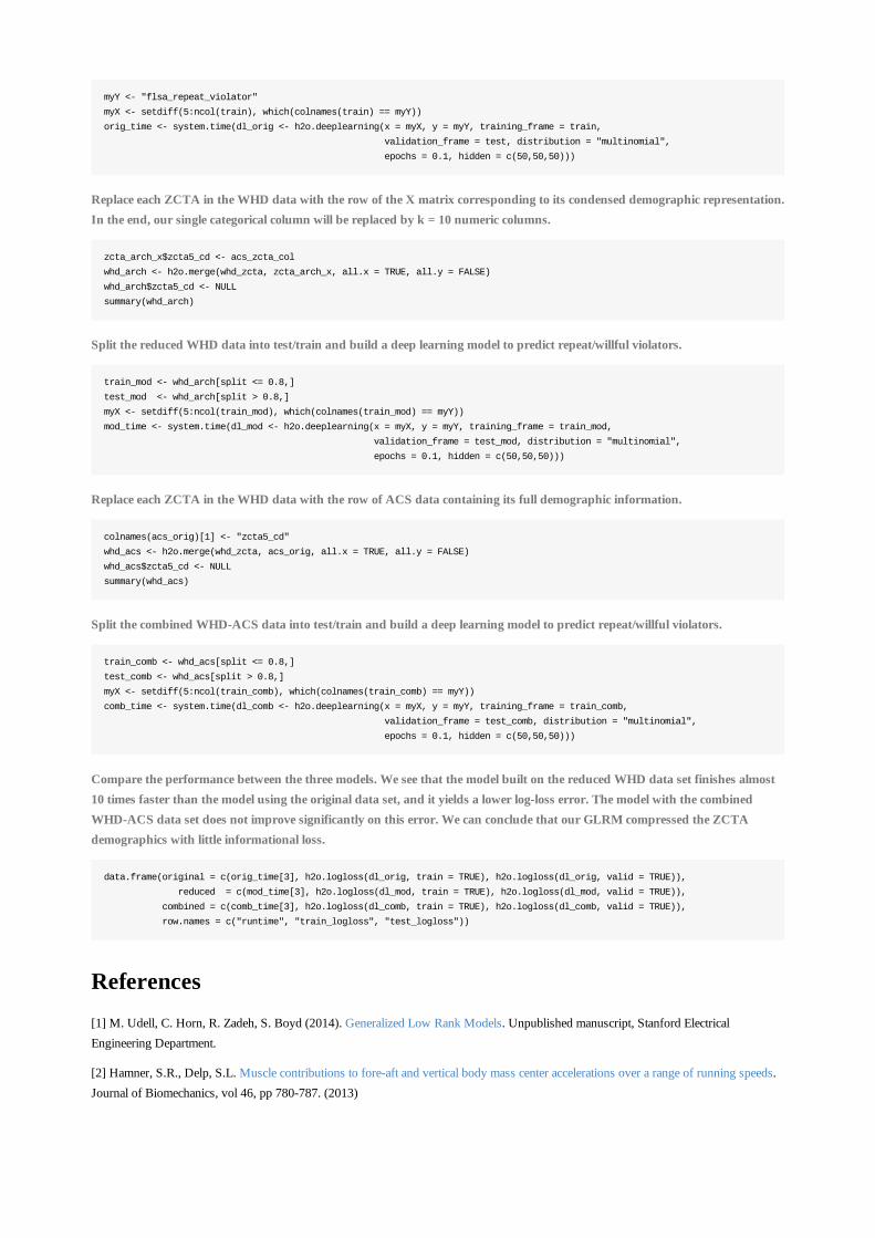
myY <- "flsa_repeat_violator"
myX <- setdiff(5:ncol(train), which(colnames(train) == myY))
orig_time <- system.time(dl_orig <- h2o.deeplearning(x = myX, y = myY, training_frame = train,
validation_frame = test, distribution = "multinomial",
epochs = 0.1, hidden = c(50,50,50)))
Replace each ZCTA in the WHD data with the row of the X matrix corresponding to its condensed demographic representation.In the end, our single categorical column will be replaced by k = 10 numeric columns.
zcta_arch_x$zcta5_cd <- acs_zcta_col
whd_arch <- h2o.merge(whd_zcta, zcta_arch_x, all.x = TRUE, all.y = FALSE)
whd_arch$zcta5_cd <- NULL
summary(whd_arch)
Split the reduced WHD data into test/train and build a deep learning model to predict repeat/willful violators.
train_mod <- whd_arch[split <= 0.8,]
test_mod <- whd_arch[split > 0.8,]
myX <- setdiff(5:ncol(train_mod), which(colnames(train_mod) == myY))
mod_time <- system.time(dl_mod <- h2o.deeplearning(x = myX, y = myY, training_frame = train_mod,
validation_frame = test_mod, distribution = "multinomial",
epochs = 0.1, hidden = c(50,50,50)))
Replace each ZCTA in the WHD data with the row of ACS data containing its full demographic information.
colnames(acs_orig)[1] <- "zcta5_cd"
whd_acs <- h2o.merge(whd_zcta, acs_orig, all.x = TRUE, all.y = FALSE)
whd_acs$zcta5_cd <- NULL
summary(whd_acs)
Split the combined WHD-ACS data into test/train and build a deep learning model to predict repeat/willful violators.
train_comb <- whd_acs[split <= 0.8,]
test_comb <- whd_acs[split > 0.8,]
myX <- setdiff(5:ncol(train_comb), which(colnames(train_comb) == myY))
comb_time <- system.time(dl_comb <- h2o.deeplearning(x = myX, y = myY, training_frame = train_comb,
validation_frame = test_comb, distribution = "multinomial",
epochs = 0.1, hidden = c(50,50,50)))
Compare the performance between the three models. We see that the model built on the reduced WHD data set finishes almost10 times faster than the model using the original data set, and it yields a lower log-loss error. The model with the combinedWHD-ACS data set does not improve significantly on this error. We can conclude that our GLRM compressed the ZCTAdemographics with little informational loss.
data.frame(original = c(orig_time[3], h2o.logloss(dl_orig, train = TRUE), h2o.logloss(dl_orig, valid = TRUE)),
reduced = c(mod_time[3], h2o.logloss(dl_mod, train = TRUE), h2o.logloss(dl_mod, valid = TRUE)),
combined = c(comb_time[3], h2o.logloss(dl_comb, train = TRUE), h2o.logloss(dl_comb, valid = TRUE)),
row.names = c("runtime", "train_logloss", "test_logloss"))
References[1] M. Udell, C. Horn, R. Zadeh, S. Boyd (2014). Generalized Low Rank Models. Unpublished manuscript, Stanford ElectricalEngineering Department.
[2] Hamner, S.R., Delp, S.L. Muscle contributions to fore-aft and vertical body mass center accelerations over a range of running speeds.Journal of Biomechanics, vol 46, pp 780-787. (2013)
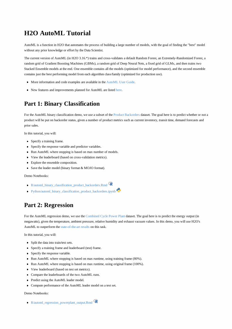
H2O AutoML TutorialAutoML is a function in H2O that automates the process of building a large number of models, with the goal of finding the "best" modelwithout any prior knowledge or effort by the Data Scientist.
The current version of AutoML (in H2O 3.16.*) trains and cross-validates a default Random Forest, an Extremely-Randomized Forest, arandom grid of Gradient Boosting Machines (GBMs), a random grid of Deep Neural Nets, a fixed grid of GLMs, and then trains twoStacked Ensemble models at the end. One ensemble contains all the models (optimized for model performance), and the second ensemblecontains just the best performing model from each algorithm class/family (optimized for production use).
More information and code examples are available in the AutoML User Guide.
New features and improvements planned for AutoML are listed here.
Part 1: Binary ClassificationFor the AutoML binary classification demo, we use a subset of the Product Backorders dataset. The goal here is to predict whether or not aproduct will be put on backorder status, given a number of product metrics such as current inventory, transit time, demand forecasts andprior sales.
In this tutorial, you will:
Specify a training frame.Specify the response variable and predictor variables.Run AutoML where stopping is based on max number of models.View the leaderboard (based on cross-validation metrics).Explore the ensemble composition.Save the leader model (binary format & MOJO format).
Demo Notebooks:
R/automl_binary_classification_product_backorders.Rmd
Python/automl_binary_classification_product_backorders.ipynb
Part 2: RegressionFor the AutoML regression demo, we use the Combined Cycle Power Plant dataset. The goal here is to predict the energy output (inmegawatts), given the temperature, ambient pressure, relative humidity and exhaust vacuum values. In this demo, you will use H2O'sAutoML to outperform the state-of-the-art results on this task.
In this tutorial, you will:
Split the data into train/test sets.Specify a training frame and leaderboard (test) frame.Specify the response variable.Run AutoML where stopping is based on max runtime, using training frame (80%).Run AutoML where stopping is based on max runtime, using original frame (100%).View leaderboard (based on test set metrics).Compare the leaderboards of the two AutoML runs.Predict using the AutoML leader model.Compute performance of the AutoML leader model on a test set.
Demo Notebooks:
R/automl_regression_powerplant_output.Rmd
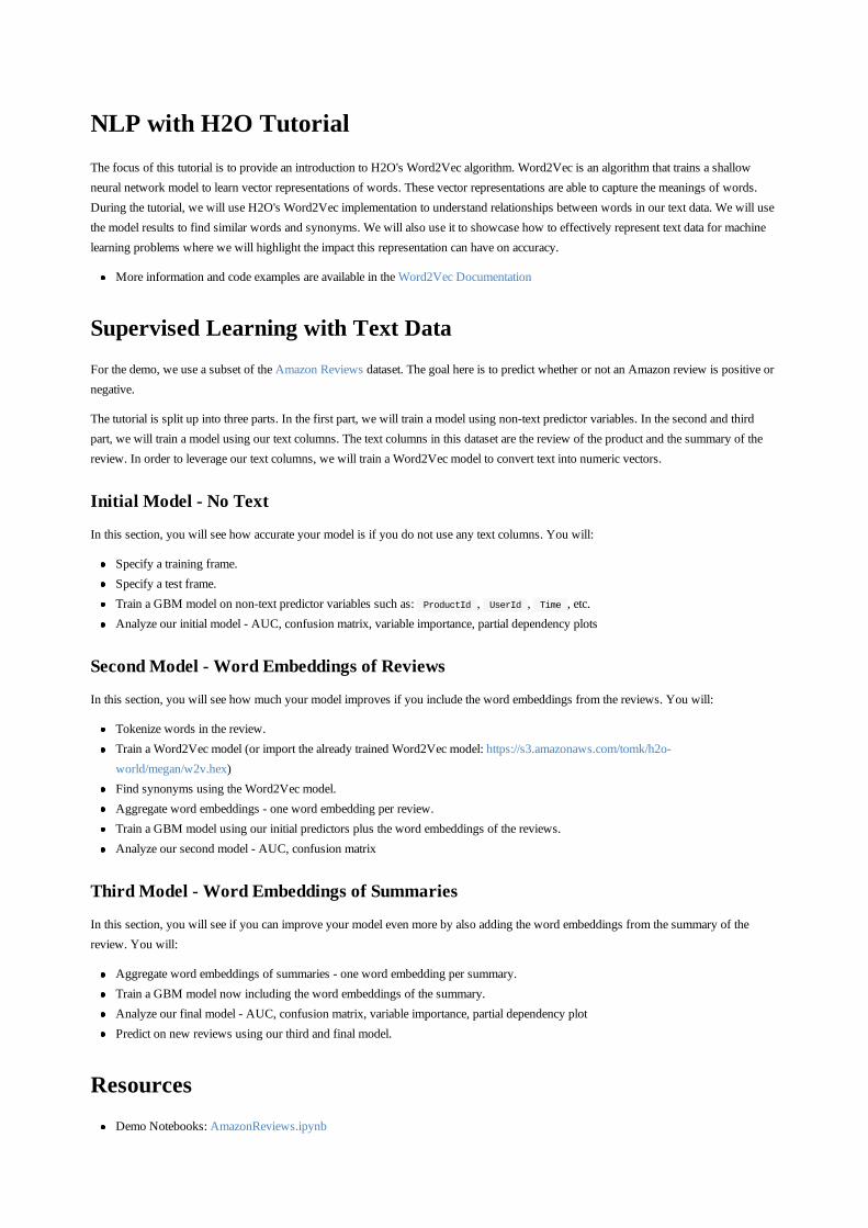
NLP with H2O TutorialThe focus of this tutorial is to provide an introduction to H2O's Word2Vec algorithm. Word2Vec is an algorithm that trains a shallowneural network model to learn vector representations of words. These vector representations are able to capture the meanings of words.During the tutorial, we will use H2O's Word2Vec implementation to understand relationships between words in our text data. We will usethe model results to find similar words and synonyms. We will also use it to showcase how to effectively represent text data for machinelearning problems where we will highlight the impact this representation can have on accuracy.
More information and code examples are available in the Word2Vec Documentation
Supervised Learning with Text DataFor the demo, we use a subset of the Amazon Reviews dataset. The goal here is to predict whether or not an Amazon review is positive ornegative.
The tutorial is split up into three parts. In the first part, we will train a model using non-text predictor variables. In the second and thirdpart, we will train a model using our text columns. The text columns in this dataset are the review of the product and the summary of thereview. In order to leverage our text columns, we will train a Word2Vec model to convert text into numeric vectors.
Initial Model - No Text
In this section, you will see how accurate your model is if you do not use any text columns. You will:
Specify a training frame.Specify a test frame.Train a GBM model on non-text predictor variables such as: ProductId , UserId , Time , etc.Analyze our initial model - AUC, confusion matrix, variable importance, partial dependency plots
Second Model - Word Embeddings of Reviews
In this section, you will see how much your model improves if you include the word embeddings from the reviews. You will:
Tokenize words in the review.Train a Word2Vec model (or import the already trained Word2Vec model: https://s3.amazonaws.com/tomk/h2o-world/megan/w2v.hex)Find synonyms using the Word2Vec model.Aggregate word embeddings - one word embedding per review.Train a GBM model using our initial predictors plus the word embeddings of the reviews.Analyze our second model - AUC, confusion matrix
Third Model - Word Embeddings of Summaries
In this section, you will see if you can improve your model even more by also adding the word embeddings from the summary of thereview. You will:
Aggregate word embeddings of summaries - one word embedding per summary.Train a GBM model now including the word embeddings of the summary.Analyze our final model - AUC, confusion matrix, variable importance, partial dependency plotPredict on new reviews using our third and final model.
ResourcesDemo Notebooks: AmazonReviews.ipynb

The subset of the Amazon Reviews data used for this demo can be found here: https://s3.amazonaws.com/tomk/h2o-world/megan/AmazonReviews.csvThe word2vec model that was trained on this data can be found here: https://s3.amazonaws.com/tomk/h2o-world/megan/w2v.hex
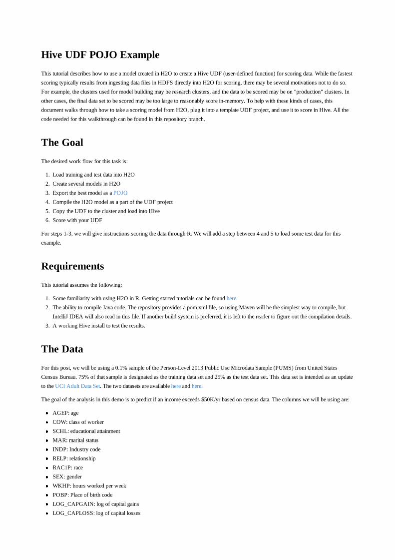
Hive UDF POJO ExampleThis tutorial describes how to use a model created in H2O to create a Hive UDF (user-defined function) for scoring data. While the fastestscoring typically results from ingesting data files in HDFS directly into H2O for scoring, there may be several motivations not to do so.For example, the clusters used for model building may be research clusters, and the data to be scored may be on "production" clusters. Inother cases, the final data set to be scored may be too large to reasonably score in-memory. To help with these kinds of cases, thisdocument walks through how to take a scoring model from H2O, plug it into a template UDF project, and use it to score in Hive. All thecode needed for this walkthrough can be found in this repository branch.
The GoalThe desired work flow for this task is:
1. Load training and test data into H2O2. Create several models in H2O3. Export the best model as a POJO4. Compile the H2O model as a part of the UDF project5. Copy the UDF to the cluster and load into Hive6. Score with your UDF
For steps 1-3, we will give instructions scoring the data through R. We will add a step between 4 and 5 to load some test data for thisexample.
RequirementsThis tutorial assumes the following:
1. Some familiarity with using H2O in R. Getting started tutorials can be found here.2. The ability to compile Java code. The repository provides a pom.xml file, so using Maven will be the simplest way to compile, but
IntelliJ IDEA will also read in this file. If another build system is preferred, it is left to the reader to figure out the compilation details.3. A working Hive install to test the results.
The DataFor this post, we will be using a 0.1% sample of the Person-Level 2013 Public Use Microdata Sample (PUMS) from United StatesCensus Bureau. 75% of that sample is designated as the training data set and 25% as the test data set. This data set is intended as an updateto the UCI Adult Data Set. The two datasets are available here and here.
The goal of the analysis in this demo is to predict if an income exceeds $50K/yr based on census data. The columns we will be using are:
AGEP: ageCOW: class of workerSCHL: educational attainmentMAR: marital statusINDP: Industry codeRELP: relationshipRAC1P: raceSEX: genderWKHP: hours worked per weekPOBP: Place of birth codeLOG_CAPGAIN: log of capital gainsLOG_CAPLOSS: log of capital losses
LOG_WAGP: log of wages or salary
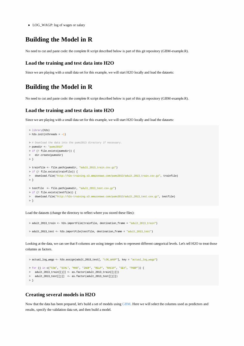
Building the Model in RNo need to cut and paste code: the complete R script described below is part of this git repository (GBM-example.R).
Load the training and test data into H2O
Since we are playing with a small data set for this example, we will start H2O locally and load the datasets:
Building the Model in RNo need to cut and paste code: the complete R script described below is part of this git repository (GBM-example.R).
Load the training and test data into H2O
Since we are playing with a small data set for this example, we will start H2O locally and load the datasets:
> library(h2o)
> h2o.init(nthreads = -1)
> # Download the data into the pums2013 directory if necessary.
> pumsdir <- "pums2013"
> if (! file.exists(pumsdir)) {
> dir.create(pumsdir)
> }
> trainfile <- file.path(pumsdir, "adult_2013_train.csv.gz")
> if (! file.exists(trainfile)) {
> download.file("http://h2o-training.s3.amazonaws.com/pums2013/adult_2013_train.csv.gz", trainfile)
> }
> testfile <- file.path(pumsdir, "adult_2013_test.csv.gz")
> if (! file.exists(testfile)) {
> download.file("http://h2o-training.s3.amazonaws.com/pums2013/adult_2013_test.csv.gz", testfile)
> }
Load the datasets (change the directory to reflect where you stored these files):
> adult_2013_train <- h2o.importFile(trainfile, destination_frame = "adult_2013_train")
> adult_2013_test <- h2o.importFile(testfile, destination_frame = "adult_2013_test")
Looking at the data, we can see that 8 columns are using integer codes to represent different categorical levels. Let's tell H2O to treat thosecolumns as factors.
> actual_log_wagp <- h2o.assign(adult_2013_test[, "LOG_WAGP"], key = "actual_log_wagp")
> for (j in c("COW", "SCHL", "MAR", "INDP", "RELP", "RAC1P", "SEX", "POBP")) {
> adult_2013_train[[j]] <- as.factor(adult_2013_train[[j]])
> adult_2013_test[[j]] <- as.factor(adult_2013_test[[j]])
> }
Creating several models in H2O
Now that the data has been prepared, let's build a set of models using GBM. Here we will select the columns used as predictors andresults, specify the validation data set, and then build a model.
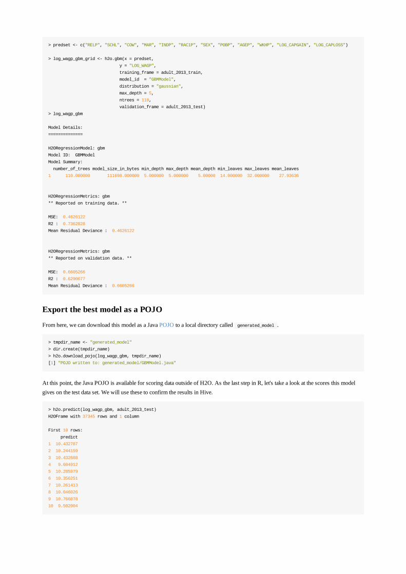
> predset <- c("RELP", "SCHL", "COW", "MAR", "INDP", "RAC1P", "SEX", "POBP", "AGEP", "WKHP", "LOG_CAPGAIN", "LOG_CAPLOSS")
> log_wagp_gbm_grid <- h2o.gbm(x = predset,
y = "LOG_WAGP",
training_frame = adult_2013_train,
model_id = "GBMModel",
distribution = "gaussian",
max_depth = 5,
ntrees = 110,
validation_frame = adult_2013_test)
> log_wagp_gbm
Model Details:
==============
H2ORegressionModel: gbm
Model ID: GBMModel
Model Summary:
number_of_trees model_size_in_bytes min_depth max_depth mean_depth min_leaves max_leaves mean_leaves
1 110.000000 111698.000000 5.000000 5.000000 5.00000 14.000000 32.000000 27.93636
H2ORegressionMetrics: gbm
** Reported on training data. **
MSE: 0.4626122
R2 : 0.7362828
Mean Residual Deviance : 0.4626122
H2ORegressionMetrics: gbm
** Reported on validation data. **
MSE: 0.6605266
R2 : 0.6290677
Mean Residual Deviance : 0.6605266
Export the best model as a POJO
From here, we can download this model as a Java POJO to a local directory called generated_model .
> tmpdir_name <- "generated_model"
> dir.create(tmpdir_name)
> h2o.download_pojo(log_wagp_gbm, tmpdir_name)
[1] "POJO written to: generated_model/GBMModel.java"
At this point, the Java POJO is available for scoring data outside of H2O. As the last step in R, let's take a look at the scores this modelgives on the test data set. We will use these to confirm the results in Hive.
> h2o.predict(log_wagp_gbm, adult_2013_test)
H2OFrame with 37345 rows and 1 column
First 10 rows:
predict
1 10.432787
2 10.244159
3 10.432688
4 9.604912
5 10.285979
6 10.356251
7 10.261413
8 10.046026
9 10.766078
10 9.502004
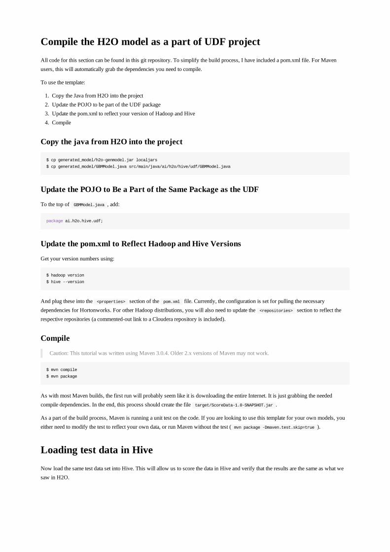
Compile the H2O model as a part of UDF projectAll code for this section can be found in this git repository. To simplify the build process, I have included a pom.xml file. For Mavenusers, this will automatically grab the dependencies you need to compile.
To use the template:
1. Copy the Java from H2O into the project2. Update the POJO to be part of the UDF package3. Update the pom.xml to reflect your version of Hadoop and Hive4. Compile
Copy the java from H2O into the project
$ cp generated_model/h2o-genmodel.jar localjars
$ cp generated_model/GBMModel.java src/main/java/ai/h2o/hive/udf/GBMModel.java
Update the POJO to Be a Part of the Same Package as the UDF
To the top of GBMModel.java , add:
package ai.h2o.hive.udf;
Update the pom.xml to Reflect Hadoop and Hive Versions
Get your version numbers using:
$ hadoop version
$ hive --version
And plug these into the <properties> section of the pom.xml file. Currently, the configuration is set for pulling the necessarydependencies for Hortonworks. For other Hadoop distributions, you will also need to update the <repositories> section to reflect therespective repositories (a commented-out link to a Cloudera repository is included).
Compile
Caution: This tutorial was written using Maven 3.0.4. Older 2.x versions of Maven may not work.
$ mvn compile
$ mvn package
As with most Maven builds, the first run will probably seem like it is downloading the entire Internet. It is just grabbing the neededcompile dependencies. In the end, this process should create the file target/ScoreData-1.0-SNAPSHOT.jar .
As a part of the build process, Maven is running a unit test on the code. If you are looking to use this template for your own models, youeither need to modify the test to reflect your own data, or run Maven without the test ( mvn package -Dmaven.test.skip=true ).
Loading test data in HiveNow load the same test data set into Hive. This will allow us to score the data in Hive and verify that the results are the same as what wesaw in H2O.
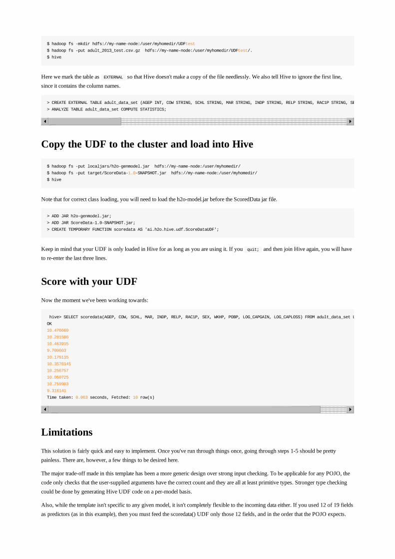
$ hadoop fs -mkdir hdfs://my-name-node:/user/myhomedir/UDFtest
$ hadoop fs -put adult_2013_test.csv.gz hdfs://my-name-node:/user/myhomedir/UDFtest/.
$ hive
Here we mark the table as EXTERNAL so that Hive doesn't make a copy of the file needlessly. We also tell Hive to ignore the first line,since it contains the column names.
> CREATE EXTERNAL TABLE adult_data_set (AGEP INT, COW STRING, SCHL STRING, MAR STRING, INDP STRING, RELP STRING, RAC1P STRING, SEX STRING, WKHP INT, POBP STRING, WAGP INT, CAPGAIN INT, CAPLOSS INT, LOG_CAPGAIN DOUBLE, LOG_CAPLOSS DOUBLE, LOG_WAGP DOUBLE, CENT_WAGP STRING, TOP_WAG2P INT, RELP_SCHL STRING) COMMENT 'PUMS 2013 test data' ROW FORMAT DELIMITED FIELDS TERMINATED BY ',' STORED AS TEXTFILE location '/user/myhomedir/UDFtest' tblproperties ("skip.header.line.count"="1");
> ANALYZE TABLE adult_data_set COMPUTE STATISTICS;
Copy the UDF to the cluster and load into Hive
$ hadoop fs -put localjars/h2o-genmodel.jar hdfs://my-name-node:/user/myhomedir/
$ hadoop fs -put target/ScoreData-1.0-SNAPSHOT.jar hdfs://my-name-node:/user/myhomedir/
$ hive
Note that for correct class loading, you will need to load the h2o-model.jar before the ScoredData jar file.
> ADD JAR h2o-genmodel.jar;
> ADD JAR ScoreData-1.0-SNAPSHOT.jar;
> CREATE TEMPORARY FUNCTION scoredata AS 'ai.h2o.hive.udf.ScoreDataUDF';
Keep in mind that your UDF is only loaded in Hive for as long as you are using it. If you quit; and then join Hive again, you will haveto re-enter the last three lines.
Score with your UDFNow the moment we've been working towards:
hive> SELECT scoredata(AGEP, COW, SCHL, MAR, INDP, RELP, RAC1P, SEX, WKHP, POBP, LOG_CAPGAIN, LOG_CAPLOSS) FROM adult_data_set LIMIT
OK
10.476669
10.201586
10.463915
9.709603
10.175115
10.3576145
10.256757
10.050725
10.759903
9.316141
Time taken: 0.063 seconds, Fetched: 10 row(s)
LimitationsThis solution is fairly quick and easy to implement. Once you've run through things once, going through steps 1-5 should be prettypainless. There are, however, a few things to be desired here.
The major trade-off made in this template has been a more generic design over strong input checking. To be applicable for any POJO, thecode only checks that the user-supplied arguments have the correct count and they are all at least primitive types. Stronger type checkingcould be done by generating Hive UDF code on a per-model basis.
Also, while the template isn't specific to any given model, it isn't completely flexible to the incoming data either. If you used 12 of 19 fieldsas predictors (as in this example), then you must feed the scoredata() UDF only those 12 fields, and in the order that the POJO expects.
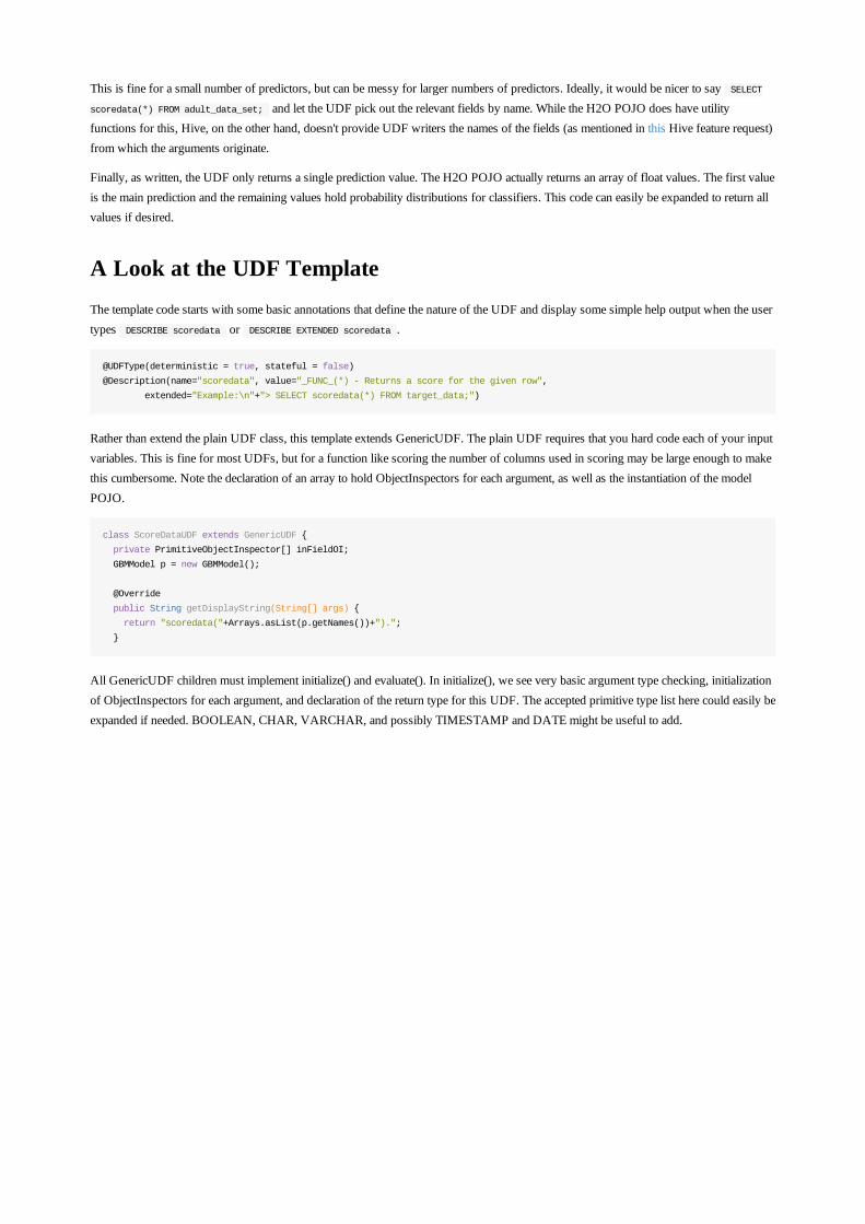
This is fine for a small number of predictors, but can be messy for larger numbers of predictors. Ideally, it would be nicer to say SELECTscoredata(*) FROM adult_data_set; and let the UDF pick out the relevant fields by name. While the H2O POJO does have utilityfunctions for this, Hive, on the other hand, doesn't provide UDF writers the names of the fields (as mentioned in this Hive feature request)from which the arguments originate.
Finally, as written, the UDF only returns a single prediction value. The H2O POJO actually returns an array of float values. The first valueis the main prediction and the remaining values hold probability distributions for classifiers. This code can easily be expanded to return allvalues if desired.
A Look at the UDF TemplateThe template code starts with some basic annotations that define the nature of the UDF and display some simple help output when the usertypes DESCRIBE scoredata or DESCRIBE EXTENDED scoredata .
@UDFType(deterministic = true, stateful = false)
@Description(name="scoredata", value="_FUNC_(*) - Returns a score for the given row",
extended="Example:\n"+"> SELECT scoredata(*) FROM target_data;")
Rather than extend the plain UDF class, this template extends GenericUDF. The plain UDF requires that you hard code each of your inputvariables. This is fine for most UDFs, but for a function like scoring the number of columns used in scoring may be large enough to makethis cumbersome. Note the declaration of an array to hold ObjectInspectors for each argument, as well as the instantiation of the modelPOJO.
class ScoreDataUDF extends GenericUDF {
private PrimitiveObjectInspector[] inFieldOI;
GBMModel p = new GBMModel();
@Override
public String getDisplayString(String[] args) {
return "scoredata("+Arrays.asList(p.getNames())+").";
}
All GenericUDF children must implement initialize() and evaluate(). In initialize(), we see very basic argument type checking, initializationof ObjectInspectors for each argument, and declaration of the return type for this UDF. The accepted primitive type list here could easily beexpanded if needed. BOOLEAN, CHAR, VARCHAR, and possibly TIMESTAMP and DATE might be useful to add.
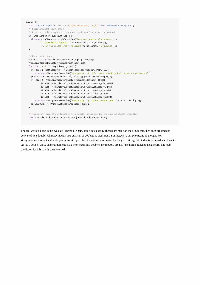
@Override
public ObjectInspector initialize(ObjectInspector[] args) throws UDFArgumentException {
// Basic argument count check
// Expects one less argument than model used; results column is dropped
if (args.length != p.getNumCols()) {
throw new UDFArgumentLengthException("Incorrect number of arguments." +
" scoredata() requires: "+ Arrays.asList(p.getNames())
+", in the listed order. Received "+args.length+" arguments.");
}
//Check input types
inFieldOI = new PrimitiveObjectInspector[args.length];
PrimitiveObjectInspector.PrimitiveCategory pCat;
for (int i = 0; i < args.length; i++) {
if (args[i].getCategory() != ObjectInspector.Category.PRIMITIVE)
throw new UDFArgumentException("scoredata(...): Only takes primitive field types as parameters");
pCat = ((PrimitiveObjectInspector) args[i]).getPrimitiveCategory();
if (pCat != PrimitiveObjectInspector.PrimitiveCategory.STRING
&& pCat != PrimitiveObjectInspector.PrimitiveCategory.DOUBLE
&& pCat != PrimitiveObjectInspector.PrimitiveCategory.FLOAT
&& pCat != PrimitiveObjectInspector.PrimitiveCategory.LONG
&& pCat != PrimitiveObjectInspector.PrimitiveCategory.INT
&& pCat != PrimitiveObjectInspector.PrimitiveCategory.SHORT)
throw new UDFArgumentException("scoredata(...): Cannot accept type: " + pCat.toString());
inFieldOI[i] = (PrimitiveObjectInspector) args[i];
}
// the return type of our function is a double, so we provide the correct object inspector
return PrimitiveObjectInspectorFactory.javaDoubleObjectInspector;
}
The real work is done in the evaluate() method. Again, some quick sanity checks are made on the arguments, then each argument isconverted to a double. All H2O models take an array of doubles as their input. For integers, a simple casting is enough. Forstrings/enumerations, the double quotes are stripped, then the enumeration value for the given string/field index is retrieved, and then it iscast to a double. Once all the arguments have been made into doubles, the model's predict() method is called to get a score. The mainprediction for this row is then returned.

@Override
public Object evaluate(DeferredObject[] record) throws HiveException {
// Expects one less argument than model used; results column is dropped
if (record != null) {
if (record.length == p.getNumCols()) {
double[] data = new double[record.length];
//Sadly, HIVE UDF doesn't currently make the field name available.
//Thus this UDF must depend solely on the arguments maintaining the same
// field order seen by the original H2O model creation.
for (int i = 0; i < record.length; i++) {
try {
Object o = inFieldOI[i].getPrimitiveJavaObject(record[i].get());
if (o instanceof java.lang.String) {
// Hive wraps strings in double quotes, remove
data[i] = p.mapEnum(i, ((String) o).replace("\"", ""));
if (data[i] == -1)
throw new UDFArgumentException("scoredata(...): The value " + (String) o
+ " is not a known category for column " + p.getNames()[i]);
} else if (o instanceof Double) {
data[i] = ((Double) o).doubleValue();
} else if (o instanceof Float) {
data[i] = ((Float) o).doubleValue();
} else if (o instanceof Long) {
data[i] = ((Long) o).doubleValue();
} else if (o instanceof Integer) {
data[i] = ((Integer) o).doubleValue();
} else if (o instanceof Short) {
data[i] = ((Short) o).doubleValue();
} else if (o == null) {
return null;
} else {
throw new UDFArgumentException("scoredata(...): Cannot accept type: "
+ o.getClass().toString() + " for argument # " + i + ".");
}
} catch (Throwable e) {
throw new UDFArgumentException("Unexpected exception on argument # " + i + ". " + e.toString());
}
}
// get the predictions
try {
double[] preds = new double[p.getPredsSize()];
p.score0(data, preds);
return preds[0];
} catch (Throwable e) {
throw new UDFArgumentException("H2O predict function threw exception: " + e.toString());
}
} else {
throw new UDFArgumentException("Incorrect number of arguments." +
" scoredata() requires: " + Arrays.asList(p.getNames()) + ", in order. Received "
+record.length+" arguments.");
}
} else { // record == null
return null; //throw new UDFArgumentException("scoredata() received a NULL row.");
}
}
Really, almost all the work is in type detection and conversion.
SummaryThat's it. The given template should work for most cases. As mentioned in the limitations section, two major modifications could be done.Some users may desire handling for a few more primitive types. Other users might want stricter type checking. There are two options forthe latter: either use the template as the basis for auto-generating type checking UDF code on a per model basis, or create a Hive clientapplication and call the UDF from the client. A Hive client could handle type checking and field alignment, since it would both see the tablelevel information and invoke the UDF.
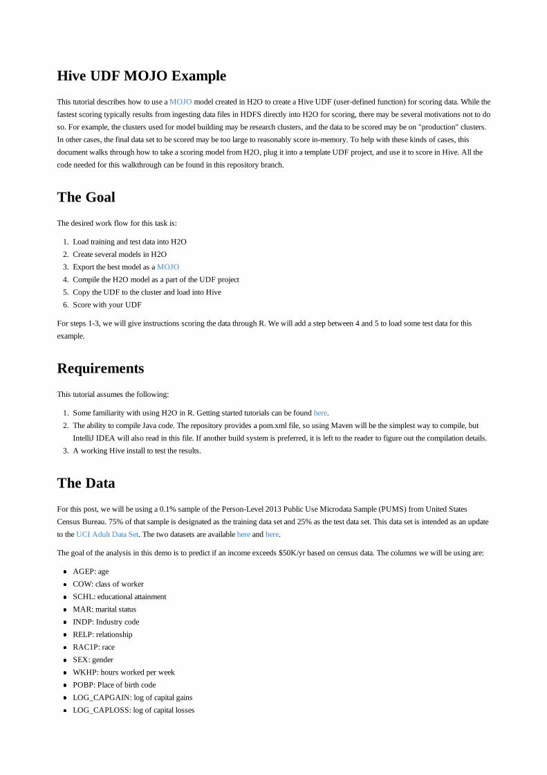
Hive UDF MOJO ExampleThis tutorial describes how to use a MOJO model created in H2O to create a Hive UDF (user-defined function) for scoring data. While thefastest scoring typically results from ingesting data files in HDFS directly into H2O for scoring, there may be several motivations not to doso. For example, the clusters used for model building may be research clusters, and the data to be scored may be on "production" clusters.In other cases, the final data set to be scored may be too large to reasonably score in-memory. To help with these kinds of cases, thisdocument walks through how to take a scoring model from H2O, plug it into a template UDF project, and use it to score in Hive. All thecode needed for this walkthrough can be found in this repository branch.
The GoalThe desired work flow for this task is:
1. Load training and test data into H2O2. Create several models in H2O3. Export the best model as a MOJO4. Compile the H2O model as a part of the UDF project5. Copy the UDF to the cluster and load into Hive6. Score with your UDF
For steps 1-3, we will give instructions scoring the data through R. We will add a step between 4 and 5 to load some test data for thisexample.
RequirementsThis tutorial assumes the following:
1. Some familiarity with using H2O in R. Getting started tutorials can be found here.2. The ability to compile Java code. The repository provides a pom.xml file, so using Maven will be the simplest way to compile, but
IntelliJ IDEA will also read in this file. If another build system is preferred, it is left to the reader to figure out the compilation details.3. A working Hive install to test the results.
The DataFor this post, we will be using a 0.1% sample of the Person-Level 2013 Public Use Microdata Sample (PUMS) from United StatesCensus Bureau. 75% of that sample is designated as the training data set and 25% as the test data set. This data set is intended as an updateto the UCI Adult Data Set. The two datasets are available here and here.
The goal of the analysis in this demo is to predict if an income exceeds $50K/yr based on census data. The columns we will be using are:
AGEP: ageCOW: class of workerSCHL: educational attainmentMAR: marital statusINDP: Industry codeRELP: relationshipRAC1P: raceSEX: genderWKHP: hours worked per weekPOBP: Place of birth codeLOG_CAPGAIN: log of capital gainsLOG_CAPLOSS: log of capital losses
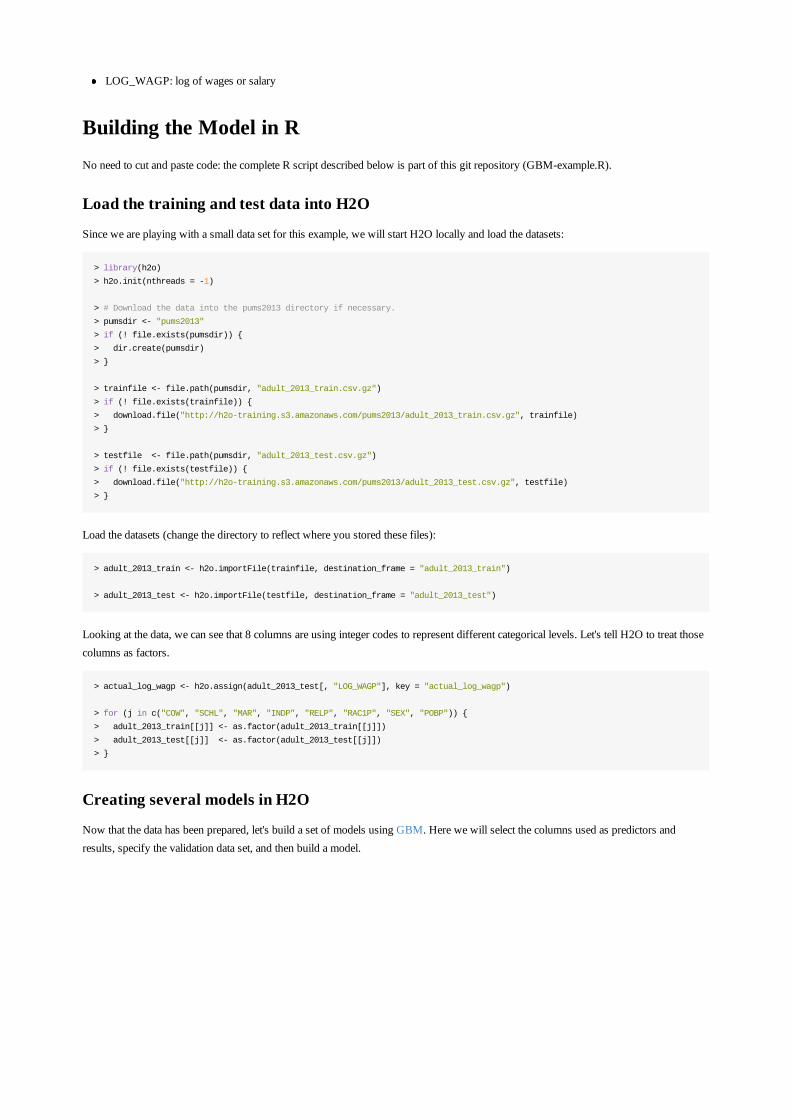
LOG_WAGP: log of wages or salary
Building the Model in RNo need to cut and paste code: the complete R script described below is part of this git repository (GBM-example.R).
Load the training and test data into H2O
Since we are playing with a small data set for this example, we will start H2O locally and load the datasets:
> library(h2o)
> h2o.init(nthreads = -1)
> # Download the data into the pums2013 directory if necessary.
> pumsdir <- "pums2013"
> if (! file.exists(pumsdir)) {
> dir.create(pumsdir)
> }
> trainfile <- file.path(pumsdir, "adult_2013_train.csv.gz")
> if (! file.exists(trainfile)) {
> download.file("http://h2o-training.s3.amazonaws.com/pums2013/adult_2013_train.csv.gz", trainfile)
> }
> testfile <- file.path(pumsdir, "adult_2013_test.csv.gz")
> if (! file.exists(testfile)) {
> download.file("http://h2o-training.s3.amazonaws.com/pums2013/adult_2013_test.csv.gz", testfile)
> }
Load the datasets (change the directory to reflect where you stored these files):
> adult_2013_train <- h2o.importFile(trainfile, destination_frame = "adult_2013_train")
> adult_2013_test <- h2o.importFile(testfile, destination_frame = "adult_2013_test")
Looking at the data, we can see that 8 columns are using integer codes to represent different categorical levels. Let's tell H2O to treat thosecolumns as factors.
> actual_log_wagp <- h2o.assign(adult_2013_test[, "LOG_WAGP"], key = "actual_log_wagp")
> for (j in c("COW", "SCHL", "MAR", "INDP", "RELP", "RAC1P", "SEX", "POBP")) {
> adult_2013_train[[j]] <- as.factor(adult_2013_train[[j]])
> adult_2013_test[[j]] <- as.factor(adult_2013_test[[j]])
> }
Creating several models in H2O
Now that the data has been prepared, let's build a set of models using GBM. Here we will select the columns used as predictors andresults, specify the validation data set, and then build a model.
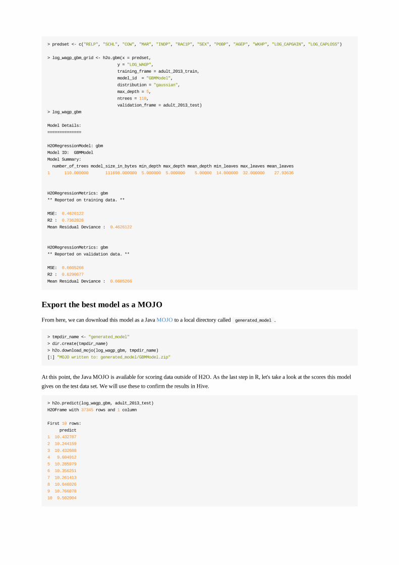
> predset <- c("RELP", "SCHL", "COW", "MAR", "INDP", "RAC1P", "SEX", "POBP", "AGEP", "WKHP", "LOG_CAPGAIN", "LOG_CAPLOSS")
> log_wagp_gbm_grid <- h2o.gbm(x = predset,
y = "LOG_WAGP",
training_frame = adult_2013_train,
model_id = "GBMModel",
distribution = "gaussian",
max_depth = 5,
ntrees = 110,
validation_frame = adult_2013_test)
> log_wagp_gbm
Model Details:
==============
H2ORegressionModel: gbm
Model ID: GBMModel
Model Summary:
number_of_trees model_size_in_bytes min_depth max_depth mean_depth min_leaves max_leaves mean_leaves
1 110.000000 111698.000000 5.000000 5.000000 5.00000 14.000000 32.000000 27.93636
H2ORegressionMetrics: gbm
** Reported on training data. **
MSE: 0.4626122
R2 : 0.7362828
Mean Residual Deviance : 0.4626122
H2ORegressionMetrics: gbm
** Reported on validation data. **
MSE: 0.6605266
R2 : 0.6290677
Mean Residual Deviance : 0.6605266
Export the best model as a MOJO
From here, we can download this model as a Java MOJO to a local directory called generated_model .
> tmpdir_name <- "generated_model"
> dir.create(tmpdir_name)
> h2o.download_mojo(log_wagp_gbm, tmpdir_name)
[1] "MOJO written to: generated_model/GBMModel.zip"
At this point, the Java MOJO is available for scoring data outside of H2O. As the last step in R, let's take a look at the scores this modelgives on the test data set. We will use these to confirm the results in Hive.
> h2o.predict(log_wagp_gbm, adult_2013_test)
H2OFrame with 37345 rows and 1 column
First 10 rows:
predict
1 10.432787
2 10.244159
3 10.432688
4 9.604912
5 10.285979
6 10.356251
7 10.261413
8 10.046026
9 10.766078
10 9.502004
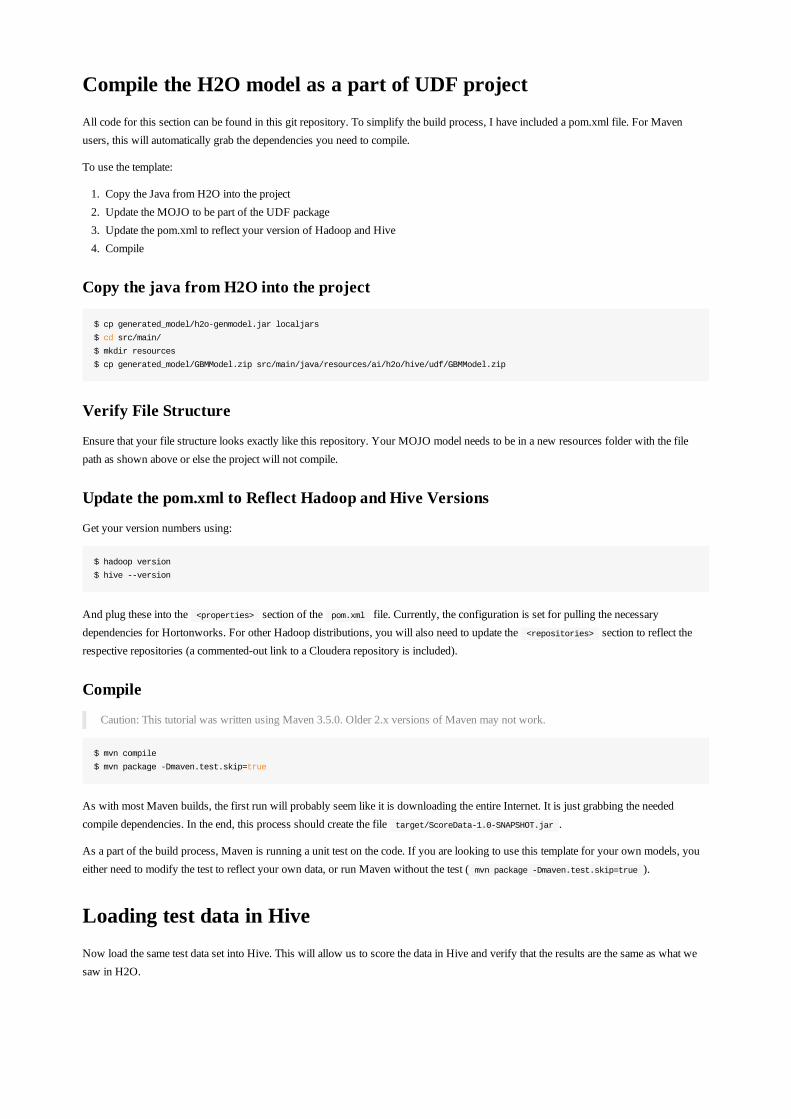
Compile the H2O model as a part of UDF projectAll code for this section can be found in this git repository. To simplify the build process, I have included a pom.xml file. For Mavenusers, this will automatically grab the dependencies you need to compile.
To use the template:
1. Copy the Java from H2O into the project2. Update the MOJO to be part of the UDF package3. Update the pom.xml to reflect your version of Hadoop and Hive4. Compile
Copy the java from H2O into the project
$ cp generated_model/h2o-genmodel.jar localjars
$ cd src/main/
$ mkdir resources
$ cp generated_model/GBMModel.zip src/main/java/resources/ai/h2o/hive/udf/GBMModel.zip
Verify File Structure
Ensure that your file structure looks exactly like this repository. Your MOJO model needs to be in a new resources folder with the filepath as shown above or else the project will not compile.
Update the pom.xml to Reflect Hadoop and Hive Versions
Get your version numbers using:
$ hadoop version
$ hive --version
And plug these into the <properties> section of the pom.xml file. Currently, the configuration is set for pulling the necessarydependencies for Hortonworks. For other Hadoop distributions, you will also need to update the <repositories> section to reflect therespective repositories (a commented-out link to a Cloudera repository is included).
Compile
Caution: This tutorial was written using Maven 3.5.0. Older 2.x versions of Maven may not work.
$ mvn compile
$ mvn package -Dmaven.test.skip=true
As with most Maven builds, the first run will probably seem like it is downloading the entire Internet. It is just grabbing the neededcompile dependencies. In the end, this process should create the file target/ScoreData-1.0-SNAPSHOT.jar .
As a part of the build process, Maven is running a unit test on the code. If you are looking to use this template for your own models, youeither need to modify the test to reflect your own data, or run Maven without the test ( mvn package -Dmaven.test.skip=true ).
Loading test data in HiveNow load the same test data set into Hive. This will allow us to score the data in Hive and verify that the results are the same as what wesaw in H2O.
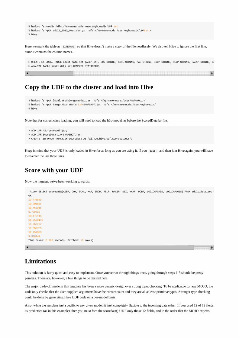
$ hadoop fs -mkdir hdfs://my-name-node:/user/myhomedir/UDFtest
$ hadoop fs -put adult_2013_test.csv.gz hdfs://my-name-node:/user/myhomedir/UDFtest/.
$ hive
Here we mark the table as EXTERNAL so that Hive doesn't make a copy of the file needlessly. We also tell Hive to ignore the first line,since it contains the column names.
> CREATE EXTERNAL TABLE adult_data_set (AGEP INT, COW STRING, SCHL STRING, MAR STRING, INDP STRING, RELP STRING, RAC1P STRING, SEX STRING, WKHP INT, POBP STRING, WAGP INT, CAPGAIN INT, CAPLOSS INT, LOG_CAPGAIN DOUBLE, LOG_CAPLOSS DOUBLE, LOG_WAGP DOUBLE, CENT_WAGP STRING, TOP_WAG2P INT, RELP_SCHL STRING) COMMENT 'PUMS 2013 test data' ROW FORMAT DELIMITED FIELDS TERMINATED BY ',' STORED AS TEXTFILE location '/user/myhomedir/UDFtest' tblproperties ("skip.header.line.count"="1");
> ANALYZE TABLE adult_data_set COMPUTE STATISTICS;
Copy the UDF to the cluster and load into Hive
$ hadoop fs -put localjars/h2o-genmodel.jar hdfs://my-name-node:/user/myhomedir/
$ hadoop fs -put target/ScoreData-1.0-SNAPSHOT.jar hdfs://my-name-node:/user/myhomedir/
$ hive
Note that for correct class loading, you will need to load the h2o-model.jar before the ScoredData jar file.
> ADD JAR h2o-genmodel.jar;
> ADD JAR ScoreData-1.0-SNAPSHOT.jar;
> CREATE TEMPORARY FUNCTION scoredata AS 'ai.h2o.hive.udf.ScoreDataUDF';
Keep in mind that your UDF is only loaded in Hive for as long as you are using it. If you quit; and then join Hive again, you will haveto re-enter the last three lines.
Score with your UDFNow the moment we've been working towards:
hive> SELECT scoredata(AGEP, COW, SCHL, MAR, INDP, RELP, RAC1P, SEX, WKHP, POBP, LOG_CAPGAIN, LOG_CAPLOSS) FROM adult_data_set LIMIT
OK
10.476669
10.201586
10.463915
9.709603
10.175115
10.3576145
10.256757
10.050725
10.759903
9.316141
Time taken: 0.063 seconds, Fetched: 10 row(s)
LimitationsThis solution is fairly quick and easy to implement. Once you've run through things once, going through steps 1-5 should be prettypainless. There are, however, a few things to be desired here.
The major trade-off made in this template has been a more generic design over strong input checking. To be applicable for any MOJO, thecode only checks that the user-supplied arguments have the correct count and they are all at least primitive types. Stronger type checkingcould be done by generating Hive UDF code on a per-model basis.
Also, while the template isn't specific to any given model, it isn't completely flexible to the incoming data either. If you used 12 of 19 fieldsas predictors (as in this example), then you must feed the scoredata() UDF only those 12 fields, and in the order that the MOJO expects.
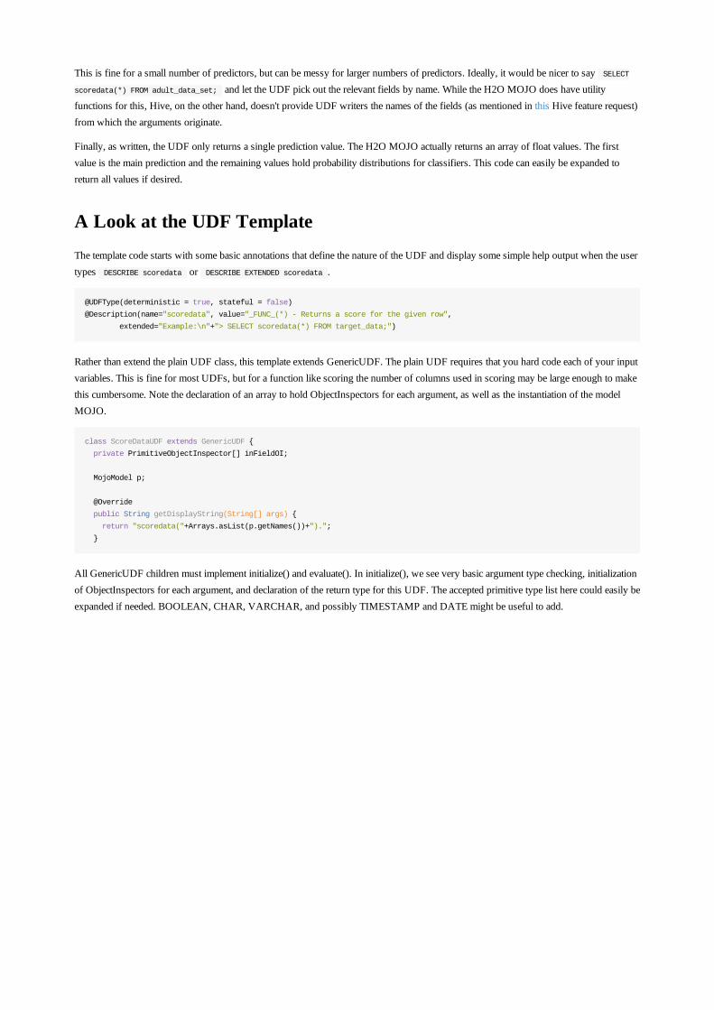
This is fine for a small number of predictors, but can be messy for larger numbers of predictors. Ideally, it would be nicer to say SELECTscoredata(*) FROM adult_data_set; and let the UDF pick out the relevant fields by name. While the H2O MOJO does have utilityfunctions for this, Hive, on the other hand, doesn't provide UDF writers the names of the fields (as mentioned in this Hive feature request)from which the arguments originate.
Finally, as written, the UDF only returns a single prediction value. The H2O MOJO actually returns an array of float values. The firstvalue is the main prediction and the remaining values hold probability distributions for classifiers. This code can easily be expanded toreturn all values if desired.
A Look at the UDF TemplateThe template code starts with some basic annotations that define the nature of the UDF and display some simple help output when the usertypes DESCRIBE scoredata or DESCRIBE EXTENDED scoredata .
@UDFType(deterministic = true, stateful = false)
@Description(name="scoredata", value="_FUNC_(*) - Returns a score for the given row",
extended="Example:\n"+"> SELECT scoredata(*) FROM target_data;")
Rather than extend the plain UDF class, this template extends GenericUDF. The plain UDF requires that you hard code each of your inputvariables. This is fine for most UDFs, but for a function like scoring the number of columns used in scoring may be large enough to makethis cumbersome. Note the declaration of an array to hold ObjectInspectors for each argument, as well as the instantiation of the modelMOJO.
class ScoreDataUDF extends GenericUDF {
private PrimitiveObjectInspector[] inFieldOI;
MojoModel p;
@Override
public String getDisplayString(String[] args) {
return "scoredata("+Arrays.asList(p.getNames())+").";
}
All GenericUDF children must implement initialize() and evaluate(). In initialize(), we see very basic argument type checking, initializationof ObjectInspectors for each argument, and declaration of the return type for this UDF. The accepted primitive type list here could easily beexpanded if needed. BOOLEAN, CHAR, VARCHAR, and possibly TIMESTAMP and DATE might be useful to add.
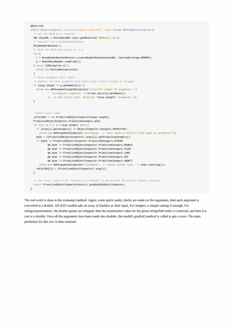
@Override
public ObjectInspector initialize(ObjectInspector[] args) throws UDFArgumentException {
// Get the MOJO as a resource
URL mojoURL = ScoreDataUDF.class.getResource("GBMModel.zip");
// Declare r as a MojoReaderBackend
MojoReaderBackend r;
// Read the MOJO and assign it to p
try {
r = MojoReaderBackendFactory.createReaderBackend(mojoURL, CachingStrategy.MEMORY);
p = ModelMojoReader.readFrom(r);
} catch (IOException e) {
throw new RuntimeException(e);
}
// Basic argument count check
// Expects one less argument than model used; results column is dropped
if (args.length != p.getNumCols()) {
throw new UDFArgumentLengthException("Incorrect number of arguments." +
" scoredata() requires: "+ Arrays.asList(p.getNames())
+", in the listed order. Received "+args.length+" arguments.");
}
//Check input types
inFieldOI = new PrimitiveObjectInspector[args.length];
PrimitiveObjectInspector.PrimitiveCategory pCat;
for (int i = 0; i < args.length; i++) {
if (args[i].getCategory() != ObjectInspector.Category.PRIMITIVE)
throw new UDFArgumentException("scoredata(...): Only takes primitive field types as parameters");
pCat = ((PrimitiveObjectInspector) args[i]).getPrimitiveCategory();
if (pCat != PrimitiveObjectInspector.PrimitiveCategory.STRING
&& pCat != PrimitiveObjectInspector.PrimitiveCategory.DOUBLE
&& pCat != PrimitiveObjectInspector.PrimitiveCategory.FLOAT
&& pCat != PrimitiveObjectInspector.PrimitiveCategory.LONG
&& pCat != PrimitiveObjectInspector.PrimitiveCategory.INT
&& pCat != PrimitiveObjectInspector.PrimitiveCategory.SHORT)
throw new UDFArgumentException("scoredata(...): Cannot accept type: " + pCat.toString());
inFieldOI[i] = (PrimitiveObjectInspector) args[i];
}
// the return type of our function is a double, so we provide the correct object inspector
return PrimitiveObjectInspectorFactory.javaDoubleObjectInspector;
}
The real work is done in the evaluate() method. Again, some quick sanity checks are made on the arguments, then each argument isconverted to a double. All H2O models take an array of doubles as their input. For integers, a simple casting is enough. Forstrings/enumerations, the double quotes are stripped, then the enumeration value for the given string/field index is retrieved, and then it iscast to a double. Once all the arguments have been made into doubles, the model's predict() method is called to get a score. The mainprediction for this row is then returned.
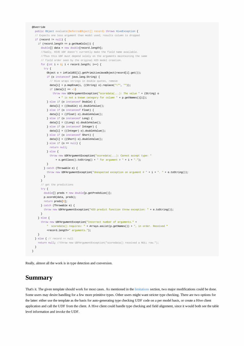
@Override
public Object evaluate(DeferredObject[] record) throws HiveException {
// Expects one less argument than model used; results column is dropped
if (record != null) {
if (record.length == p.getNumCols()) {
double[] data = new double[record.length];
//Sadly, HIVE UDF doesn't currently make the field name available.
//Thus this UDF must depend solely on the arguments maintaining the same
// field order seen by the original H2O model creation.
for (int i = 0; i < record.length; i++) {
try {
Object o = inFieldOI[i].getPrimitiveJavaObject(record[i].get());
if (o instanceof java.lang.String) {
// Hive wraps strings in double quotes, remove
data[i] = p.mapEnum(i, ((String) o).replace("\"", ""));
if (data[i] == -1)
throw new UDFArgumentException("scoredata(...): The value " + (String) o
+ " is not a known category for column " + p.getNames()[i]);
} else if (o instanceof Double) {
data[i] = ((Double) o).doubleValue();
} else if (o instanceof Float) {
data[i] = ((Float) o).doubleValue();
} else if (o instanceof Long) {
data[i] = ((Long) o).doubleValue();
} else if (o instanceof Integer) {
data[i] = ((Integer) o).doubleValue();
} else if (o instanceof Short) {
data[i] = ((Short) o).doubleValue();
} else if (o == null) {
return null;
} else {
throw new UDFArgumentException("scoredata(...): Cannot accept type: "
+ o.getClass().toString() + " for argument # " + i + ".");
}
} catch (Throwable e) {
throw new UDFArgumentException("Unexpected exception on argument # " + i + ". " + e.toString());
}
}
// get the predictions
try {
double[] preds = new double[p.getPredsSize()];
p.score0(data, preds);
return preds[0];
} catch (Throwable e) {
throw new UDFArgumentException("H2O predict function threw exception: " + e.toString());
}
} else {
throw new UDFArgumentException("Incorrect number of arguments." +
" scoredata() requires: " + Arrays.asList(p.getNames()) + ", in order. Received "
+record.length+" arguments.");
}
} else { // record == null
return null; //throw new UDFArgumentException("scoredata() received a NULL row.");
}
}
Really, almost all the work is in type detection and conversion.
SummaryThat's it. The given template should work for most cases. As mentioned in the limitations section, two major modifications could be done.Some users may desire handling for a few more primitive types. Other users might want stricter type checking. There are two options forthe latter: either use the template as the basis for auto-generating type checking UDF code on a per model basis, or create a Hive clientapplication and call the UDF from the client. A Hive client could handle type checking and field alignment, since it would both see the tablelevel information and invoke the UDF.
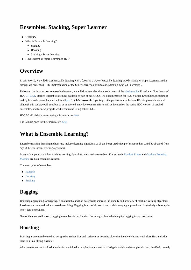
Ensembles: Stacking, Super LearnerOverviewWhat is Ensemble Learning?
BaggingBoostingStacking / Super Learning
H2O Ensemble: Super Learning in H2O
OverviewIn this tutorial, we will discuss ensemble learning with a focus on a type of ensemble learning called stacking or Super Learning. In thistutorial, we present an H2O implementation of the Super Learner algorithm (aka. Stacking, Stacked Ensembles).
Following the introduction to ensemble learning, we will dive into a hands-on code demo of the h2oEnsemble R package. Note that as ofH2O 3.10.3.1, Stacked Ensembles are now available as part of base H2O. The documentation for H2O Stacked Ensembles, including Rand Python code examples, can be found here. The h2oEnsemble R package is the predecessor to the base H2O implementation andalthough this package will contibue to be supported, new development efforts will be focused on the native H2O version of stackedensembles, and for new projects we'd recommend using native H2O.
H2O World slides accompanying this tutorial are here.
The GitHub page for the ensembles is here.
What is Ensemble Learning?Ensemble machine learning methods use multiple learning algorithms to obtain better predictive performance than could be obtained fromany of the constituent learning algorithms.
Many of the popular modern machine learning algorithms are actually ensembles. For example, Random Forest and Gradient BoostingMachine are both ensemble learners.
Common types of ensembles:
BaggingBoostingStacking
BaggingBootstrap aggregating, or bagging, is an ensemble method designed to improve the stability and accuracy of machine learning algorithms.It reduces variance and helps to avoid overfitting. Bagging is a special case of the model averaging approach and is relatively robust againstnoisy data and outliers.
One of the most well known bagging ensembles is the Random Forest algorithm, which applies bagging to decision trees.
BoostingBoosting is an ensemble method designed to reduce bias and variance. A boosting algorithm iteratively learns weak classifiers and addsthem to a final strong classifier.
After a weak learner is added, the data is reweighted: examples that are misclassified gain weight and examples that are classified correctly
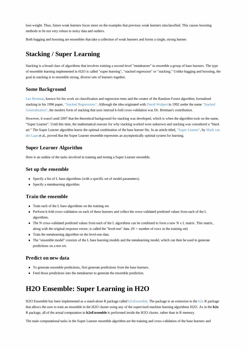
lose weight. Thus, future weak learners focus more on the examples that previous weak learners misclassified. This causes boostingmethods to be not very robust to noisy data and outliers.
Both bagging and boosting are ensembles that take a collection of weak learners and forms a single, strong learner.
Stacking / Super LearningStacking is a broad class of algorithms that involves training a second-level "metalearner" to ensemble a group of base learners. The typeof ensemble learning implemented in H2O is called "super learning", "stacked regression" or "stacking." Unlike bagging and boosting, thegoal in stacking is to ensemble strong, diverse sets of learners together.
Some Background
Leo Breiman, known for his work on classification and regression trees and the creator of the Random Forest algorithm, formalizedstacking in his 1996 paper, "Stacked Regressions". Although the idea originated with David Wolpert in 1992 under the name "StackedGeneralization", the modern form of stacking that uses internal k-fold cross-validation was Dr. Breiman's contribution.
However, it wasn't until 2007 that the theoretical background for stacking was developed, which is when the algorithm took on the name,"Super Learner". Until this time, the mathematical reasons for why stacking worked were unknown and stacking was considered a "blackart." The Super Learner algorithm learns the optimal combination of the base learner fits. In an article titled, "Super Learner", by Mark vander Laan et al., proved that the Super Learner ensemble represents an asymptotically optimal system for learning.
Super Learner Algorithm
Here is an outline of the tasks involved in training and testing a Super Learner ensemble.
Set up the ensemble
Specify a list of L base algorithms (with a specific set of model parameters).Specify a metalearning algorithm.
Train the ensemble
Train each of the L base algorithms on the training set.Perform k-fold cross-validation on each of these learners and collect the cross-validated predicted values from each of the Lalgorithms.The N cross-validated predicted values from each of the L algorithms can be combined to form a new N x L matrix. This matrix,along wtih the original response vector, is called the "level-one" data. (N = number of rows in the training set)Train the metalearning algorithm on the level-one data.The "ensemble model" consists of the L base learning models and the metalearning model, which can then be used to generatepredictions on a test set.
Predict on new data
To generate ensemble predictions, first generate predictions from the base learners.Feed those predictions into the metalearner to generate the ensemble prediction.
H2O Ensemble: Super Learning in H2OH2O Ensemble has been implemented as a stand-alone R package called h2oEnsemble. The package is an extension to the h2o R packagethat allows the user to train an ensemble in the H2O cluster using any of the supervised machine learning algorithms H2O. As in the h2oR package, all of the actual computation in h2oEnsemble is performed inside the H2O cluster, rather than in R memory.
The main computational tasks in the Super Learner ensemble algorithm are the training and cross-validation of the base learners and
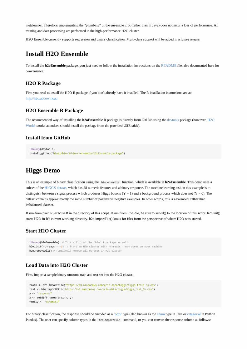
metalearner. Therefore, implementing the "plumbing" of the ensemble in R (rather than in Java) does not incur a loss of performance. Alltraining and data processing are performed in the high-performance H2O cluster.
H2O Ensemble currently supports regression and binary classification. Multi-class support will be added in a future release.
Install H2O EnsembleTo install the h2oEnsemble package, you just need to follow the installation instructions on the README file, also documented here forconvenience.
H2O R Package
First you need to install the H2O R package if you don't already have it installed. The R installation instructions are at:http://h2o.ai/download
H2O Ensemble R Package
The recommended way of installing the h2oEnsemble R package is directly from GitHub using the devtools package (however, H2OWorld tutorial attendees should install the package from the provided USB stick).
Install from GitHub
library(devtools)
install_github("h2oai/h2o-3/h2o-r/ensemble/h2oEnsemble-package")
Higgs DemoThis is an example of binary classification using the h2o.ensemble function, which is available in h2oEnsemble. This demo uses asubset of the HIGGS dataset, which has 28 numeric features and a binary response. The machine learning task in this example is todistinguish between a signal process which produces Higgs bosons (Y = 1) and a background process which does not (Y = 0). Thedataset contains approximately the same number of positive vs negative examples. In other words, this is a balanced, rather thanimbalanced, dataset.
If run from plain R, execute R in the directory of this script. If run from RStudio, be sure to setwd() to the location of this script. h2o.init()starts H2O in R's current working directory. h2o.importFile() looks for files from the perspective of where H2O was started.
Start H2O Cluster
library(h2oEnsemble) # This will load the `h2o` R package as well
h2o.init(nthreads = -1) # Start an H2O cluster with nthreads = num cores on your machine
h2o.removeAll() # (Optional) Remove all objects in H2O cluster
Load Data into H2O Cluster
First, import a sample binary outcome train and test set into the H2O cluster.
train <- h2o.importFile("https://s3.amazonaws.com/erin-data/higgs/higgs_train_5k.csv")
test <- h2o.importFile("https://s3.amazonaws.com/erin-data/higgs/higgs_test_5k.csv")
y <- "response"
x <- setdiff(names(train), y)
family <- "binomial"
For binary classification, the response should be encoded as a factor type (also known as the enum type in Java or categorial in PythonPandas). The user can specify column types in the h2o.importFile command, or you can convert the response column as follows:
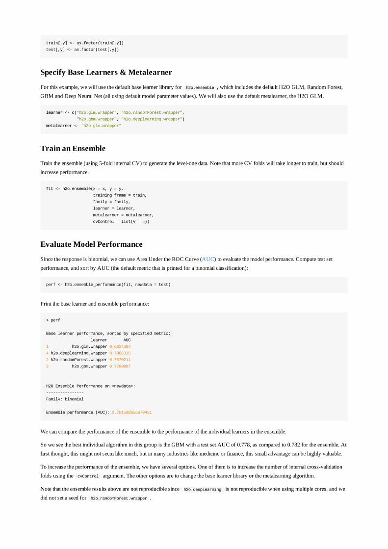
train[,y] <- as.factor(train[,y])
test[,y] <- as.factor(test[,y])
Specify Base Learners & Metalearner
For this example, we will use the default base learner library for h2o.ensemble , which includes the default H2O GLM, Random Forest,GBM and Deep Neural Net (all using default model parameter values). We will also use the default metalearner, the H2O GLM.
learner <- c("h2o.glm.wrapper", "h2o.randomForest.wrapper",
"h2o.gbm.wrapper", "h2o.deeplearning.wrapper")
metalearner <- "h2o.glm.wrapper"
Train an Ensemble
Train the ensemble (using 5-fold internal CV) to generate the level-one data. Note that more CV folds will take longer to train, but shouldincrease performance.
fit <- h2o.ensemble(x = x, y = y,
training_frame = train,
family = family,
learner = learner,
metalearner = metalearner,
cvControl = list(V = 5))
Evaluate Model Performance
Since the response is binomial, we can use Area Under the ROC Curve (AUC) to evaluate the model performance. Compute test setperformance, and sort by AUC (the default metric that is printed for a binomial classification):
perf <- h2o.ensemble_performance(fit, newdata = test)
Print the base learner and ensemble performance:
> perf
Base learner performance, sorted by specified metric:
learner AUC
1 h2o.glm.wrapper 0.6824304
4 h2o.deeplearning.wrapper 0.7006335
2 h2o.randomForest.wrapper 0.7570211
3 h2o.gbm.wrapper 0.7780807
H2O Ensemble Performance on <newdata>:
----------------
Family: binomial
Ensemble performance (AUC): 0.781580655670451
We can compare the performance of the ensemble to the performance of the individual learners in the ensemble.
So we see the best individual algorithm in this group is the GBM with a test set AUC of 0.778, as compared to 0.782 for the ensemble. Atfirst thought, this might not seem like much, but in many industries like medicine or finance, this small advantage can be highly valuable.
To increase the performance of the ensemble, we have several options. One of them is to increase the number of internal cross-validationfolds using the cvControl argument. The other options are to change the base learner library or the metalearning algorithm.
Note that the ensemble results above are not reproducible since h2o.deeplearning is not reproducible when using multiple cores, and wedid not set a seed for h2o.randomForest.wrapper .
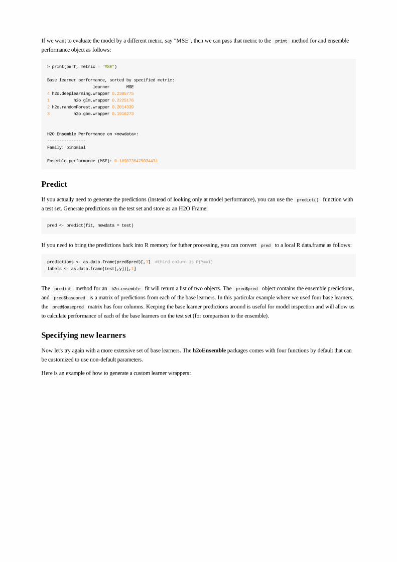
If we want to evaluate the model by a different metric, say "MSE", then we can pass that metric to the print method for and ensembleperformance object as follows:
> print(perf, metric = "MSE")
Base learner performance, sorted by specified metric:
learner MSE
4 h2o.deeplearning.wrapper 0.2305775
1 h2o.glm.wrapper 0.2225176
2 h2o.randomForest.wrapper 0.2014339
3 h2o.gbm.wrapper 0.1916273
H2O Ensemble Performance on <newdata>:
----------------
Family: binomial
Ensemble performance (MSE): 0.1898735479034431
Predict
If you actually need to generate the predictions (instead of looking only at model performance), you can use the predict() function witha test set. Generate predictions on the test set and store as an H2O Frame:
pred <- predict(fit, newdata = test)
If you need to bring the predictions back into R memory for futher processing, you can convert pred to a local R data.frame as follows:
predictions <- as.data.frame(pred$pred)[,3] #third column is P(Y==1)
labels <- as.data.frame(test[,y])[,1]
The predict method for an h2o.ensemble fit will return a list of two objects. The pred$pred object contains the ensemble predictions,and pred$basepred is a matrix of predictions from each of the base learners. In this particular example where we used four base learners,the pred$basepred matrix has four columns. Keeping the base learner predictions around is useful for model inspection and will allow usto calculate performance of each of the base learners on the test set (for comparison to the ensemble).
Specifying new learners
Now let's try again with a more extensive set of base learners. The h2oEnsemble packages comes with four functions by default that canbe customized to use non-default parameters.
Here is an example of how to generate a custom learner wrappers:
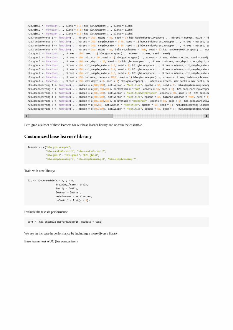
h2o.glm.1 <- function(..., alpha = 0.0) h2o.glm.wrapper(..., alpha = alpha)
h2o.glm.2 <- function(..., alpha = 0.5) h2o.glm.wrapper(..., alpha = alpha)
h2o.glm.3 <- function(..., alpha = 1.0) h2o.glm.wrapper(..., alpha = alpha)
h2o.randomForest.1 <- function(..., ntrees = 200, nbins = 50, seed = 1) h2o.randomForest.wrapper(..., ntrees = ntrees, nbins = nbins, seed = seed)
h2o.randomForest.2 <- function(..., ntrees = 200, sample_rate = 0.75, seed = 1) h2o.randomForest.wrapper(..., ntrees = ntrees, sample_rate = sample_rate, seed = seed)
h2o.randomForest.3 <- function(..., ntrees = 200, sample_rate = 0.85, seed = 1) h2o.randomForest.wrapper(..., ntrees = ntrees, sample_rate = sample_rate, seed = seed)
h2o.randomForest.4 <- function(..., ntrees = 200, nbins = 50, balance_classes = TRUE, seed = 1) h2o.randomForest.wrapper(..., ntrees = ntrees, nbins = nbins, balance_classes = balance_classes, seed = seed)
h2o.gbm.1 <- function(..., ntrees = 100, seed = 1) h2o.gbm.wrapper(..., ntrees = ntrees, seed = seed)
h2o.gbm.2 <- function(..., ntrees = 100, nbins = 50, seed = 1) h2o.gbm.wrapper(..., ntrees = ntrees, nbins = nbins, seed = seed)
h2o.gbm.3 <- function(..., ntrees = 100, max_depth = 10, seed = 1) h2o.gbm.wrapper(..., ntrees = ntrees, max_depth = max_depth, seed = seed)
h2o.gbm.4 <- function(..., ntrees = 100, col_sample_rate = 0.8, seed = 1) h2o.gbm.wrapper(..., ntrees = ntrees, col_sample_rate = col_sample_rate, seed = seed)
h2o.gbm.5 <- function(..., ntrees = 100, col_sample_rate = 0.7, seed = 1) h2o.gbm.wrapper(..., ntrees = ntrees, col_sample_rate = col_sample_rate, seed = seed)
h2o.gbm.6 <- function(..., ntrees = 100, col_sample_rate = 0.6, seed = 1) h2o.gbm.wrapper(..., ntrees = ntrees, col_sample_rate = col_sample_rate, seed = seed)
h2o.gbm.7 <- function(..., ntrees = 100, balance_classes = TRUE, seed = 1) h2o.gbm.wrapper(..., ntrees = ntrees, balance_classes = balance_classes, seed = seed)
h2o.gbm.8 <- function(..., ntrees = 100, max_depth = 3, seed = 1) h2o.gbm.wrapper(..., ntrees = ntrees, max_depth = max_depth, seed = seed)
h2o.deeplearning.1 <- function(..., hidden = c(500,500), activation = "Rectifier", epochs = 50, seed = 1) h2o.deeplearning.wrapper(
h2o.deeplearning.2 <- function(..., hidden = c(200,200,200), activation = "Tanh", epochs = 50, seed = 1) h2o.deeplearning.wrapper(
h2o.deeplearning.3 <- function(..., hidden = c(500,500), activation = "RectifierWithDropout", epochs = 50, seed = 1) h2o.deeplearning.wrapper(
h2o.deeplearning.4 <- function(..., hidden = c(500,500), activation = "Rectifier", epochs = 50, balance_classes = TRUE, seed = 1) h2o.deeplearning.wrapper(
h2o.deeplearning.5 <- function(..., hidden = c(100,100,100), activation = "Rectifier", epochs = 50, seed = 1) h2o.deeplearning.wrapper(
h2o.deeplearning.6 <- function(..., hidden = c(50,50), activation = "Rectifier", epochs = 50, seed = 1) h2o.deeplearning.wrapper(
h2o.deeplearning.7 <- function(..., hidden = c(100,100), activation = "Rectifier", epochs = 50, seed = 1) h2o.deeplearning.wrapper(
Let's grab a subset of these learners for our base learner library and re-train the ensemble.
Customized base learner library
learner <- c("h2o.glm.wrapper",
"h2o.randomForest.1", "h2o.randomForest.2",
"h2o.gbm.1", "h2o.gbm.6", "h2o.gbm.8",
"h2o.deeplearning.1", "h2o.deeplearning.6", "h2o.deeplearning.7")
Train with new library:
fit <- h2o.ensemble(x = x, y = y,
training_frame = train,
family = family,
learner = learner,
metalearner = metalearner,
cvControl = list(V = 5))
Evaluate the test set performance:
perf <- h2o.ensemble_performance(fit, newdata = test)
We see an increase in performance by including a more diverse library.
Base learner test AUC (for comparison)
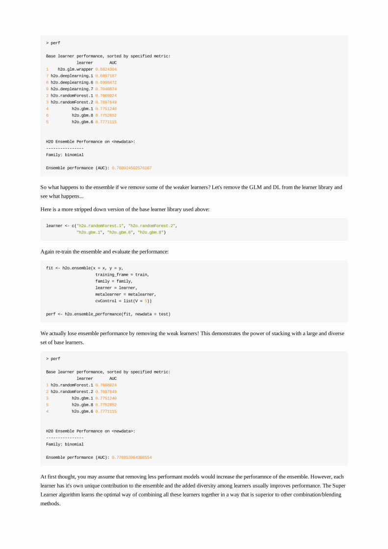
> perf
Base learner performance, sorted by specified metric:
learner AUC
1 h2o.glm.wrapper 0.6824304
7 h2o.deeplearning.1 0.6897187
8 h2o.deeplearning.6 0.6998472
9 h2o.deeplearning.7 0.7048874
2 h2o.randomForest.1 0.7668024
3 h2o.randomForest.2 0.7697849
4 h2o.gbm.1 0.7751240
6 h2o.gbm.8 0.7752852
5 h2o.gbm.6 0.7771115
H2O Ensemble Performance on <newdata>:
----------------
Family: binomial
Ensemble performance (AUC): 0.780924502576107
So what happens to the ensemble if we remove some of the weaker learners? Let's remove the GLM and DL from the learner library andsee what happens...
Here is a more stripped down version of the base learner library used above:
learner <- c("h2o.randomForest.1", "h2o.randomForest.2",
"h2o.gbm.1", "h2o.gbm.6", "h2o.gbm.8")
Again re-train the ensemble and evaluate the performance:
fit <- h2o.ensemble(x = x, y = y,
training_frame = train,
family = family,
learner = learner,
metalearner = metalearner,
cvControl = list(V = 5))
perf <- h2o.ensemble_performance(fit, newdata = test)
We actually lose ensemble performance by removing the weak learners! This demonstrates the power of stacking with a large and diverseset of base learners.
> perf
Base learner performance, sorted by specified metric:
learner AUC
1 h2o.randomForest.1 0.7668024
2 h2o.randomForest.2 0.7697849
3 h2o.gbm.1 0.7751240
5 h2o.gbm.8 0.7752852
4 h2o.gbm.6 0.7771115
H2O Ensemble Performance on <newdata>:
----------------
Family: binomial
Ensemble performance (AUC): 0.778853964308554
At first thought, you may assume that removing less performant models would increase the perforamnce of the ensemble. However, eachlearner has it's own unique contribution to the ensemble and the added diversity among learners usually improves performance. The SuperLearner algorithm learns the optimal way of combining all these learners together in a way that is superior to other combination/blendingmethods.

Stacking Existing Model Sets
You can also use an existing (cross-validated) list of H2O models as the starting point and use the h2o.stack() function to ensemblethem together via a specified metalearner. The base models must have been trained on the same dataset with same response and for cross-validation, must have all used the same folds.
An example follows. As above, start up the H2O cluster and load the training and test data.
library(h2oEnsemble)
h2o.init(nthreads = -1) # Start H2O cluster using all available CPU threads
# Import a sample binary outcome train/test set into R
train <- h2o.importFile("https://s3.amazonaws.com/erin-data/higgs/higgs_train_5k.csv")
test <- h2o.importFile("https://s3.amazonaws.com/erin-data/higgs/higgs_test_5k.csv")
y <- "response"
x <- setdiff(names(train), y)
family <- "binomial"
#For binary classification, response should be a factor
train[,y] <- as.factor(train[,y])
test[,y] <- as.factor(test[,y])
Cross-validate and train a handful of base learners and then use the h2o.stack() function to create the ensemble:
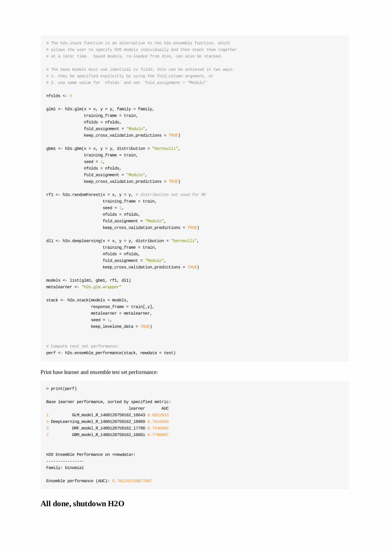
# The h2o.stack function is an alternative to the h2o.ensemble function, which
# allows the user to specify H2O models individually and then stack them together
# at a later time. Saved models, re-loaded from disk, can also be stacked.
# The base models must use identical cv folds; this can be achieved in two ways:
# 1. they be specified explicitly by using the fold_column argument, or
# 2. use same value for `nfolds` and set `fold_assignment = "Modulo"`
nfolds <- 5
glm1 <- h2o.glm(x = x, y = y, family = family,
training_frame = train,
nfolds = nfolds,
fold_assignment = "Modulo",
keep_cross_validation_predictions = TRUE)
gbm1 <- h2o.gbm(x = x, y = y, distribution = "bernoulli",
training_frame = train,
seed = 1,
nfolds = nfolds,
fold_assignment = "Modulo",
keep_cross_validation_predictions = TRUE)
rf1 <- h2o.randomForest(x = x, y = y, # distribution not used for RF
training_frame = train,
seed = 1,
nfolds = nfolds,
fold_assignment = "Modulo",
keep_cross_validation_predictions = TRUE)
dl1 <- h2o.deeplearning(x = x, y = y, distribution = "bernoulli",
training_frame = train,
nfolds = nfolds,
fold_assignment = "Modulo",
keep_cross_validation_predictions = TRUE)
models <- list(glm1, gbm1, rf1, dl1)
metalearner <- "h2o.glm.wrapper"
stack <- h2o.stack(models = models,
response_frame = train[,y],
metalearner = metalearner,
seed = 1,
keep_levelone_data = TRUE)
# Compute test set performance:
perf <- h2o.ensemble_performance(stack, newdata = test)
Print base learner and ensemble test set performance:
> print(perf)
Base learner performance, sorted by specified metric:
learner AUC
1 GLM_model_R_1480128759162_16643 0.6822933
4 DeepLearning_model_R_1480128759162_18909 0.7016809
3 DRF_model_R_1480128759162_17790 0.7546005
2 GBM_model_R_1480128759162_16661 0.7780807
H2O Ensemble Performance on <newdata>:
----------------
Family: binomial
Ensemble performance (AUC): 0.781241759877087
All done, shutdown H2O

h2o.shutdown()
Roadmap for h2oEnsembleh2oEnsemble is only available as an R package. A list of open tickets (bugs, feature requests) for the package can be found here (JIRAtickets with the "h2oEnsemble" tag).
Open tickets for the native H2O version of Stacked Ensembles can be found here (JIRA tickets with the "StackedEnsemble" tag).
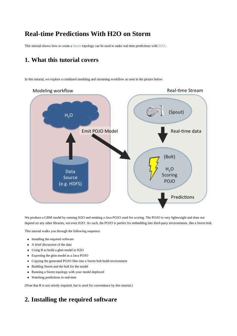
Real-time Predictions With H2O on StormThis tutorial shows how to create a Storm topology can be used to make real-time predictions with H2O.
1. What this tutorial covers
In this tutorial, we explore a combined modeling and streaming workflow as seen in the picture below:
We produce a GBM model by running H2O and emitting a Java POJO used for scoring. The POJO is very lightweight and does notdepend on any other libraries, not even H2O. As such, the POJO is perfect for embedding into third-party environments, like a Storm bolt.
This tutorial walks you through the following sequence:
Installing the required softwareA brief discussion of the dataUsing R to build a gbm model in H2OExporting the gbm model as a Java POJOCopying the generated POJO files into a Storm bolt build environmentBuilding Storm and the bolt for the modelRunning a Storm topology with your model deployedWatching predictions in real-time
(Note that R is not strictly required, but is used for convenience by this tutorial.)
2. Installing the required software
2.1. Clone the required repositories from Github
git clone https://github.com/apache/storm.git
git clone https://github.com/h2oai/h2o-world-2015-training.git
NOTE: Building storm (c.f. Section 5) requires Maven. You can install Maven (version 3.x) by following the Maven installationinstructions.
Navigate to the directory for this tutorial inside the h2o-world-2015-training repository:
cd h2o-world-2015-training/tutorials/streaming/storm
You should see the following files in this directory:
README.md (This document)example.R (The R script that builds the GBM model and exports it as a Java POJO)training_data.csv (The data used to build the GBM model)live_data.csv (The data that predictions are made on; used to feed the spout in the Storm topology)H2OStormStarter.java (The Storm topology with two bolts: a prediction bolt and a classifying bolt)TestH2ODataSpout.java (The Storm spout which reads data from the live_data.csv file and passes each observation to the predictionbolt one observation at a time; this simulates the arrival of data in real-time)
And the following directories:
premade_generated_model (For those people who have trouble building the model but want to try running with Storm anyway; youcan ignore this directory if you successfully build your own generated_model later in the tutorial)images (Images for the tutorial documentation, you can ignore these)web (Contains the html and image files for watching the real-time prediction output (c.f. Section 8))
2.2. Install R
Get the latest version of R from CRAN and install it on your computer.
2.3. Install the H2O package for R
Note: The H2O package for R includes both the R code as well as the main H2O jar file. This is all you need to run H2O locally onyour laptop.
Step 1: Start R (at the command line or via RStudio)
Step 2: Install H2O from CRAN
install.packages("h2o")
Note: For convenience, this tutorial was created with the Slater stable release of H2O (3.2.0.3) from CRAN, as shown above. Laterversions of H2O will also work.
2.4. Development environment
This tutorial was developed with the following software environment. (Other environments will work, but this is what we used to developand test this tutorial.)
H2O 3.3.0.99999 (Slater)MacOS X (Mavericks)java version "1.7.0_79"R 3.2.2Storm git hash: 99285bb719357760f572d6f4f0fb4cd02a8fd389
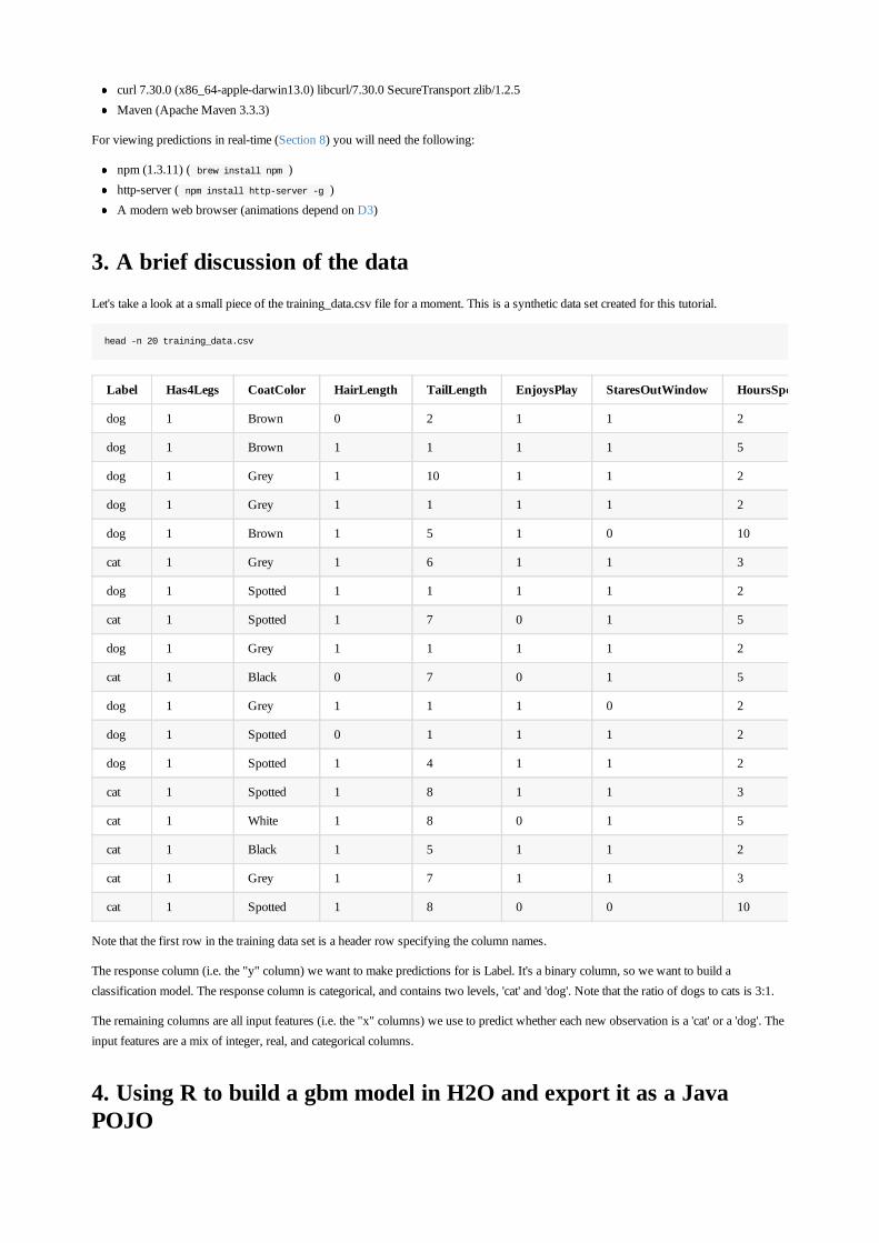
curl 7.30.0 (x86_64-apple-darwin13.0) libcurl/7.30.0 SecureTransport zlib/1.2.5Maven (Apache Maven 3.3.3)
For viewing predictions in real-time (Section 8) you will need the following:
npm (1.3.11) ( brew install npm )http-server ( npm install http-server -g )A modern web browser (animations depend on D3)
3. A brief discussion of the dataLet's take a look at a small piece of the training_data.csv file for a moment. This is a synthetic data set created for this tutorial.
head -n 20 training_data.csv
Label Has4Legs CoatColor HairLength TailLength EnjoysPlay StaresOutWindow HoursSpentNapping
dog 1 Brown 0 2 1 1 2
dog 1 Brown 1 1 1 1 5
dog 1 Grey 1 10 1 1 2
dog 1 Grey 1 1 1 1 2
dog 1 Brown 1 5 1 0 10
cat 1 Grey 1 6 1 1 3
dog 1 Spotted 1 1 1 1 2
cat 1 Spotted 1 7 0 1 5
dog 1 Grey 1 1 1 1 2
cat 1 Black 0 7 0 1 5
dog 1 Grey 1 1 1 0 2
dog 1 Spotted 0 1 1 1 2
dog 1 Spotted 1 4 1 1 2
cat 1 Spotted 1 8 1 1 3
cat 1 White 1 8 0 1 5
cat 1 Black 1 5 1 1 2
cat 1 Grey 1 7 1 1 3
cat 1 Spotted 1 8 0 0 10
Note that the first row in the training data set is a header row specifying the column names.
The response column (i.e. the "y" column) we want to make predictions for is Label. It's a binary column, so we want to build aclassification model. The response column is categorical, and contains two levels, 'cat' and 'dog'. Note that the ratio of dogs to cats is 3:1.
The remaining columns are all input features (i.e. the "x" columns) we use to predict whether each new observation is a 'cat' or a 'dog'. Theinput features are a mix of integer, real, and categorical columns.
4. Using R to build a gbm model in H2O and export it as a JavaPOJO
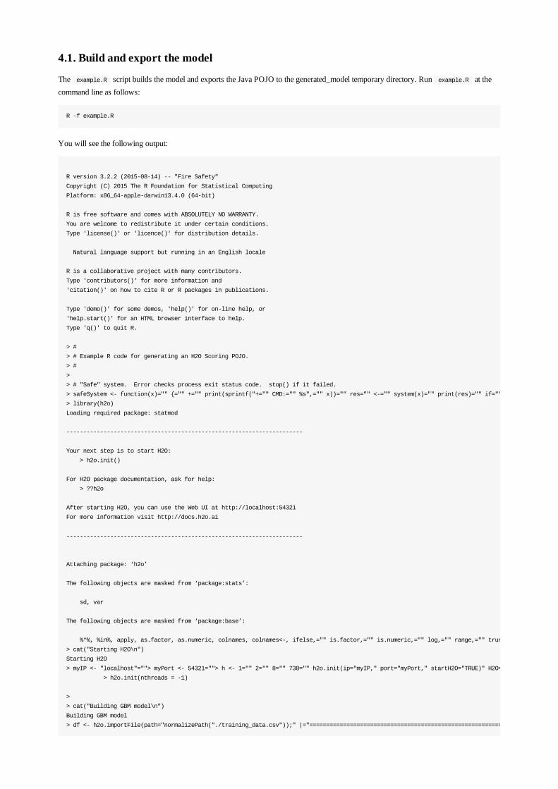
4.1. Build and export the model
The example.R script builds the model and exports the Java POJO to the generated_model temporary directory. Run example.R at thecommand line as follows:
R -f example.R
You will see the following output:
R version 3.2.2 (2015-08-14) -- "Fire Safety"
Copyright (C) 2015 The R Foundation for Statistical Computing
Platform: x86_64-apple-darwin13.4.0 (64-bit)
R is free software and comes with ABSOLUTELY NO WARRANTY.
You are welcome to redistribute it under certain conditions.
Type 'license()' or 'licence()' for distribution details.
Natural language support but running in an English locale
R is a collaborative project with many contributors.
Type 'contributors()' for more information and
'citation()' on how to cite R or R packages in publications.
Type 'demo()' for some demos, 'help()' for on-line help, or
'help.start()' for an HTML browser interface to help.
Type 'q()' to quit R.
> #
> # Example R code for generating an H2O Scoring POJO.
> #
>
> # "Safe" system. Error checks process exit status code. stop() if it failed.
> safeSystem <- function(x)="" {="" +="" print(sprintf("+="" CMD:="" %s",="" x))="" res="" <-="" system(x)="" print(res)="" if="" (res="" !="0)" msg="" sprintf("SYSTEM="" COMMAND="" FAILED="" (exit="" status="" %d)",="" res)="" stop(msg)="" }="">
> library(h2o)
Loading required package: statmod
----------------------------------------------------------------------
Your next step is to start H2O:
> h2o.init()
For H2O package documentation, ask for help:
> ??h2o
After starting H2O, you can use the Web UI at http://localhost:54321
For more information visit http://docs.h2o.ai
----------------------------------------------------------------------
Attaching package: ‘h2o’
The following objects are masked from ‘package:stats’:
sd, var
The following objects are masked from ‘package:base’:
%*%, %in%, apply, as.factor, as.numeric, colnames, colnames<-, ifelse,="" is.factor,="" is.numeric,="" log,="" range,="" trunc="">
> cat("Starting H2O\n")
Starting H2O
> myIP <- "localhost"=""> myPort <- 54321=""> h <- 1="" 2="" 8="" 738="" h2o.init(ip="myIP," port="myPort," startH2O="TRUE)" H2O="" is="" not="" running="" yet,="" starting="" it="" now...="" Note:="" In="" case="" of="" errors="" look="" at="" the="" following="" log="" files:="" var="" folders="" ct="" mv0lk53d5lq6bkvm_2snjgm00000gn="" T="" RtmpkEUbAR="" h2o_ludirehak_started_from_r.out="" h2o_ludirehak_started_from_r.err="" java="" version="" "1.7.0_79"="" Java(TM)="" SE="" Runtime="" Environment="" (build="" 1.7.0_79-b15)="" Java="" HotSpot(TM)="" 64-Bit="" Server="" VM="" 24.79-b02,="" mixed="" mode)="" ..Successfully="" connected="" to="" http:="" localhost:54321="" R="" cluster:="" cluster="" uptime:="" seconds="" milliseconds="" version:="" 3.3.0.99999="" name:="" H2O_started_from_R_ludirehak_dwh703="" total="" nodes:="" memory:="" 3.56="" GB="" cores:="" allowed="" healthy:="" TRUE="" As="" started,="" limited="" CRAN="" default CPUs.="" Shut="" down="" and="" restart="" as="" shown="" below="" use="" all="" your=""> h2o.shutdown()
> h2o.init(nthreads = -1)
>
> cat("Building GBM model\n")
Building GBM model
> df <- h2o.importFile(path="normalizePath("./training_data.csv"));" |="=====================================================================|" 100%=""> y <- "Label"=""> x <- c("Has4Legs","CoatColor","HairLength","TailLength","EnjoysPlay","StaresOutWindow","HoursSpentNapping","RespondsToCommands","EasilyFrightened","Age",="" "Noise1",="" "Noise2",="" "Noise3",="" "Noise4",="" "Noise5")=""> gbm.h2o.fit <- h2o.gbm(training_frame="df," y="y," x="x," model_id="GBMPojo" ,="" ntrees="10)" |="=====================================================================|" 100%="">
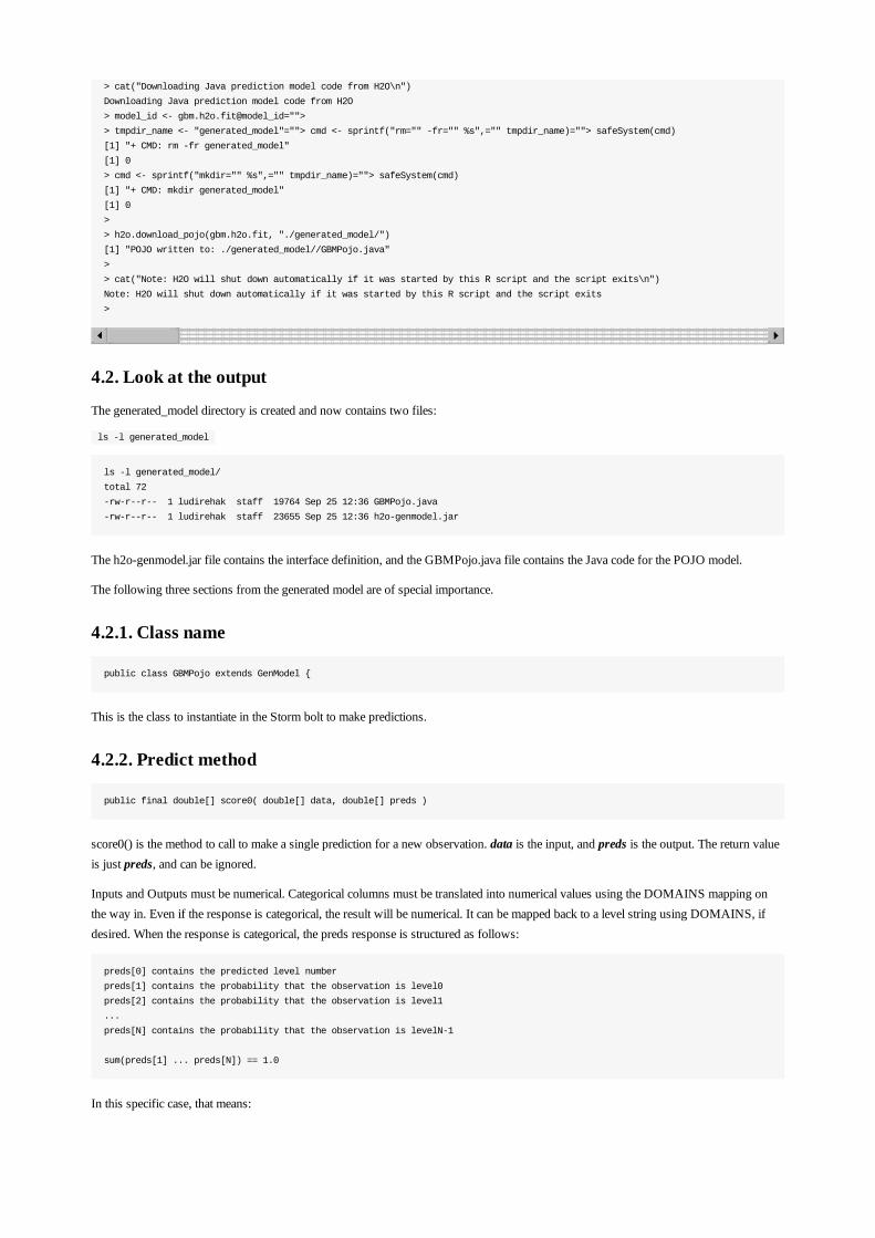
> cat("Downloading Java prediction model code from H2O\n")
Downloading Java prediction model code from H2O
> model_id <- gbm.h2o.fit@model_id="">
> tmpdir_name <- "generated_model"=""> cmd <- sprintf("rm="" -fr="" %s",="" tmpdir_name)=""> safeSystem(cmd)
[1] "+ CMD: rm -fr generated_model"
[1] 0
> cmd <- sprintf("mkdir="" %s",="" tmpdir_name)=""> safeSystem(cmd)
[1] "+ CMD: mkdir generated_model"
[1] 0
>
> h2o.download_pojo(gbm.h2o.fit, "./generated_model/")
[1] "POJO written to: ./generated_model//GBMPojo.java"
>
> cat("Note: H2O will shut down automatically if it was started by this R script and the script exits\n")
Note: H2O will shut down automatically if it was started by this R script and the script exits
>
4.2. Look at the output
The generated_model directory is created and now contains two files:
ls -l generated_model
ls -l generated_model/
total 72
-rw-r--r-- 1 ludirehak staff 19764 Sep 25 12:36 GBMPojo.java
-rw-r--r-- 1 ludirehak staff 23655 Sep 25 12:36 h2o-genmodel.jar
The h2o-genmodel.jar file contains the interface definition, and the GBMPojo.java file contains the Java code for the POJO model.
The following three sections from the generated model are of special importance.
4.2.1. Class name
public class GBMPojo extends GenModel {
This is the class to instantiate in the Storm bolt to make predictions.
4.2.2. Predict method
public final double[] score0( double[] data, double[] preds )
score0() is the method to call to make a single prediction for a new observation. data is the input, and preds is the output. The return valueis just preds, and can be ignored.
Inputs and Outputs must be numerical. Categorical columns must be translated into numerical values using the DOMAINS mapping onthe way in. Even if the response is categorical, the result will be numerical. It can be mapped back to a level string using DOMAINS, ifdesired. When the response is categorical, the preds response is structured as follows:
preds[0] contains the predicted level number
preds[1] contains the probability that the observation is level0
preds[2] contains the probability that the observation is level1
...
preds[N] contains the probability that the observation is levelN-1
sum(preds[1] ... preds[N]) == 1.0
In this specific case, that means:
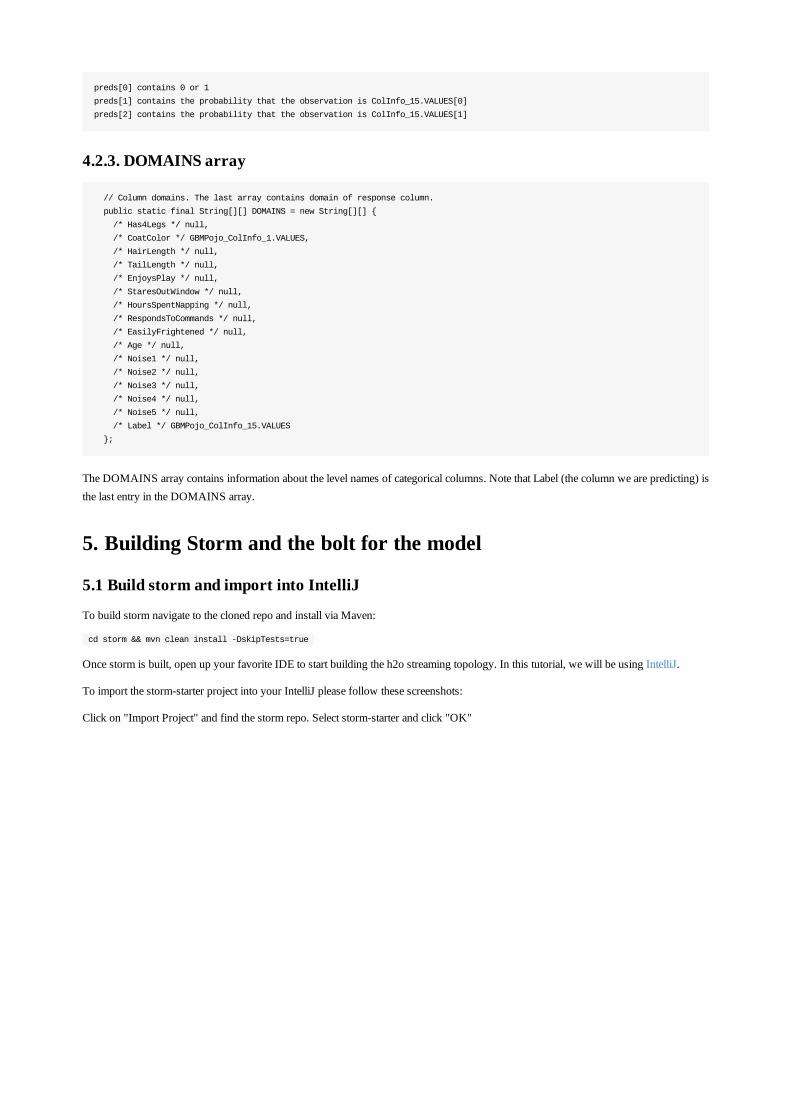
preds[0] contains 0 or 1
preds[1] contains the probability that the observation is ColInfo_15.VALUES[0]
preds[2] contains the probability that the observation is ColInfo_15.VALUES[1]
4.2.3. DOMAINS array
// Column domains. The last array contains domain of response column.
public static final String[][] DOMAINS = new String[][] {
/* Has4Legs */ null,
/* CoatColor */ GBMPojo_ColInfo_1.VALUES,
/* HairLength */ null,
/* TailLength */ null,
/* EnjoysPlay */ null,
/* StaresOutWindow */ null,
/* HoursSpentNapping */ null,
/* RespondsToCommands */ null,
/* EasilyFrightened */ null,
/* Age */ null,
/* Noise1 */ null,
/* Noise2 */ null,
/* Noise3 */ null,
/* Noise4 */ null,
/* Noise5 */ null,
/* Label */ GBMPojo_ColInfo_15.VALUES
};
The DOMAINS array contains information about the level names of categorical columns. Note that Label (the column we are predicting) isthe last entry in the DOMAINS array.
5. Building Storm and the bolt for the model
5.1 Build storm and import into IntelliJ
To build storm navigate to the cloned repo and install via Maven:
cd storm && mvn clean install -DskipTests=true
Once storm is built, open up your favorite IDE to start building the h2o streaming topology. In this tutorial, we will be using IntelliJ.
To import the storm-starter project into your IntelliJ please follow these screenshots:
Click on "Import Project" and find the storm repo. Select storm-starter and click "OK"
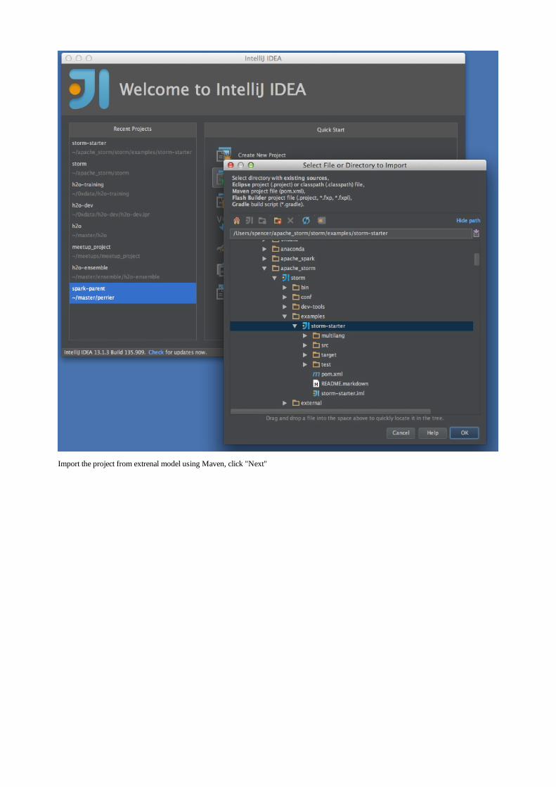
Import the project from extrenal model using Maven, click "Next"

Ensure that "Import Maven projects automatically" check box is clicked (it's off by default), click "Next"
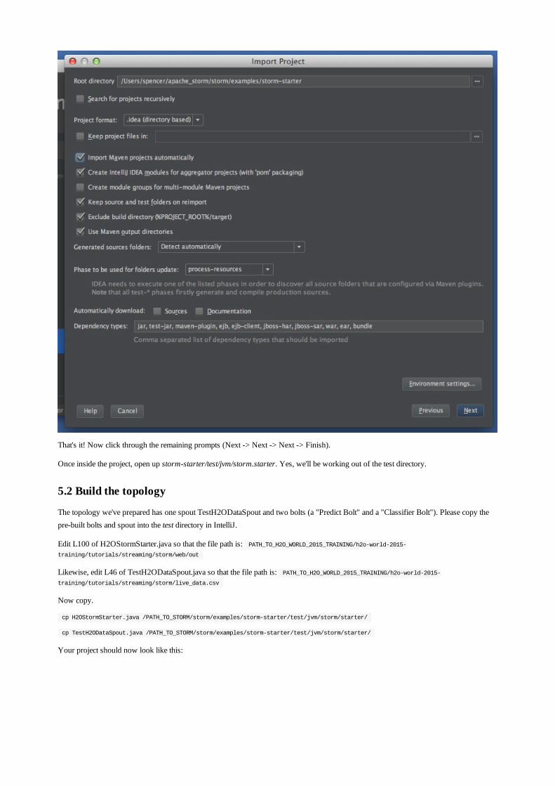
That's it! Now click through the remaining prompts (Next -> Next -> Next -> Finish).
Once inside the project, open up storm-starter/test/jvm/storm.starter. Yes, we'll be working out of the test directory.
5.2 Build the topology
The topology we've prepared has one spout TestH2ODataSpout and two bolts (a "Predict Bolt" and a "Classifier Bolt"). Please copy thepre-built bolts and spout into the test directory in IntelliJ.
Edit L100 of H2OStormStarter.java so that the file path is: PATH_TO_H2O_WORLD_2015_TRAINING/h2o-world-2015-training/tutorials/streaming/storm/web/out
Likewise, edit L46 of TestH2ODataSpout.java so that the file path is: PATH_TO_H2O_WORLD_2015_TRAINING/h2o-world-2015-training/tutorials/streaming/storm/live_data.csv
Now copy.
cp H2OStormStarter.java /PATH_TO_STORM/storm/examples/storm-starter/test/jvm/storm/starter/
cp TestH2ODataSpout.java /PATH_TO_STORM/storm/examples/storm-starter/test/jvm/storm/starter/
Your project should now look like this:

6. Copying the generated POJO files into a Storm bolt buildenvironmentWe are now ready to import the H2O pieces into the IntelliJ project. We'll need to add the h2o-genmodel.jar and the scoring POJO.
To import the h2o-genmodel.jar into your IntelliJ project, please follow these screenshots:
File > Project Structure…

Click the "+" to add a new dependency
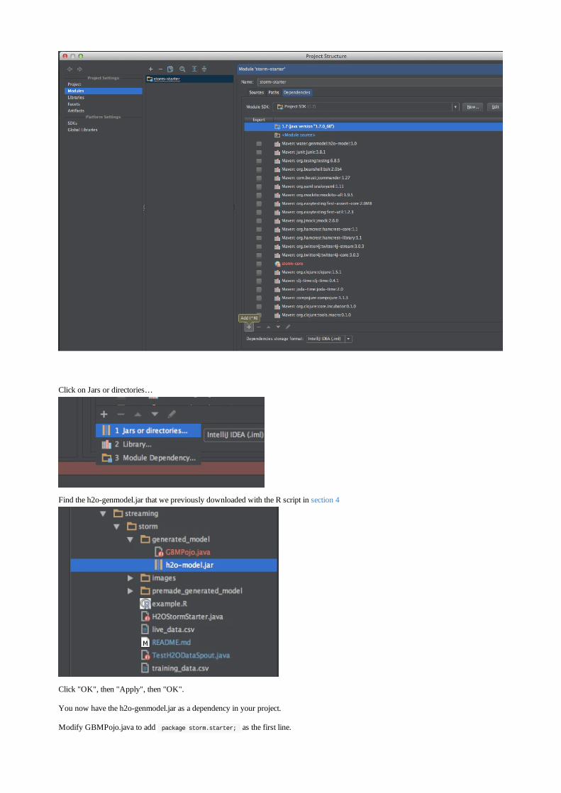
Click on Jars or directories…
Find the h2o-genmodel.jar that we previously downloaded with the R script in section 4
Click "OK", then "Apply", then "OK".
You now have the h2o-genmodel.jar as a dependency in your project.
Modify GBMPojo.java to add package storm.starter; as the first line.
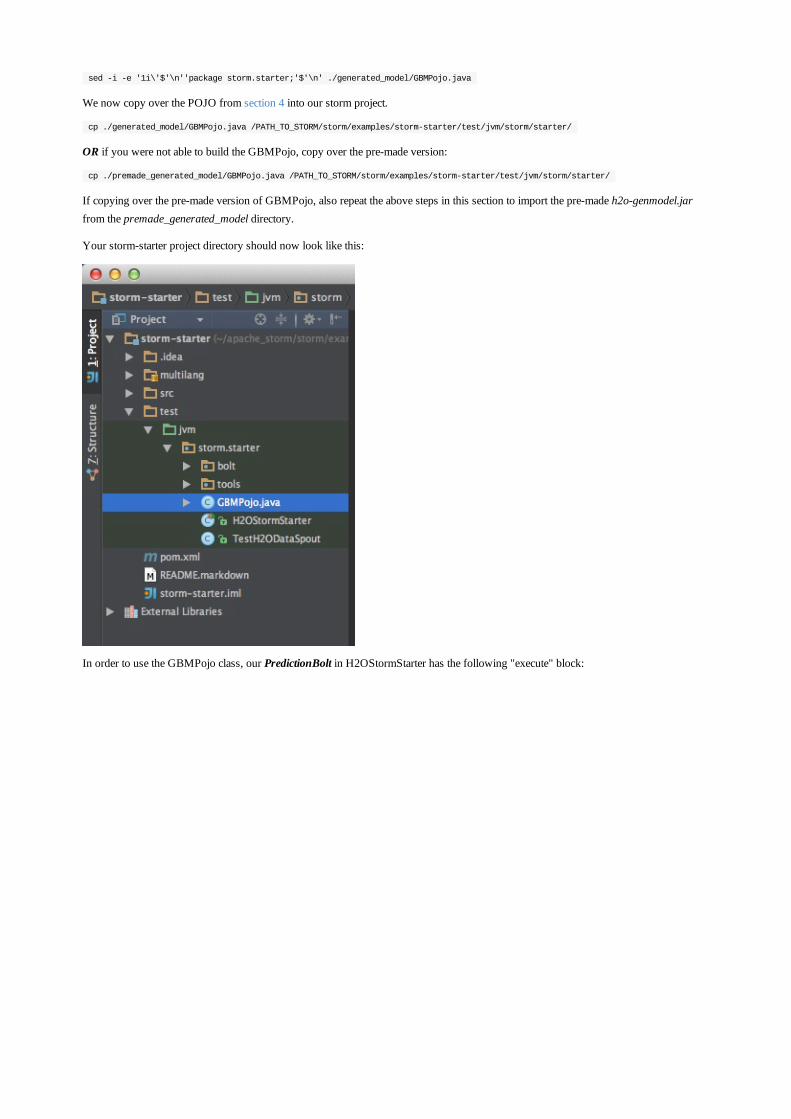
sed -i -e '1i\'$'\n''package storm.starter;'$'\n' ./generated_model/GBMPojo.java
We now copy over the POJO from section 4 into our storm project.
cp ./generated_model/GBMPojo.java /PATH_TO_STORM/storm/examples/storm-starter/test/jvm/storm/starter/
OR if you were not able to build the GBMPojo, copy over the pre-made version:
cp ./premade_generated_model/GBMPojo.java /PATH_TO_STORM/storm/examples/storm-starter/test/jvm/storm/starter/
If copying over the pre-made version of GBMPojo, also repeat the above steps in this section to import the pre-made h2o-genmodel.jarfrom the premade_generated_model directory.
Your storm-starter project directory should now look like this:
In order to use the GBMPojo class, our PredictionBolt in H2OStormStarter has the following "execute" block:
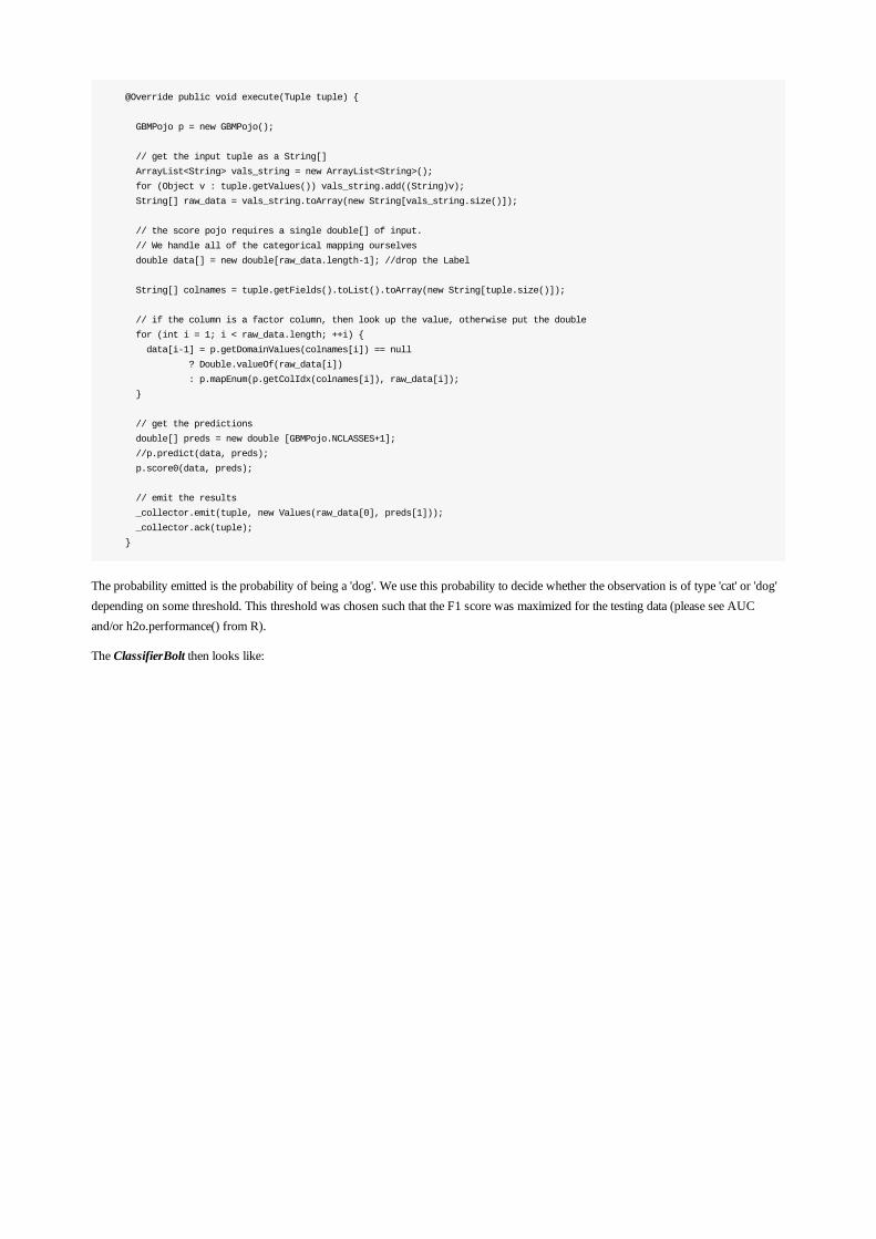
@Override public void execute(Tuple tuple) {
GBMPojo p = new GBMPojo();
// get the input tuple as a String[]
ArrayList<String> vals_string = new ArrayList<String>();
for (Object v : tuple.getValues()) vals_string.add((String)v);
String[] raw_data = vals_string.toArray(new String[vals_string.size()]);
// the score pojo requires a single double[] of input.
// We handle all of the categorical mapping ourselves
double data[] = new double[raw_data.length-1]; //drop the Label
String[] colnames = tuple.getFields().toList().toArray(new String[tuple.size()]);
// if the column is a factor column, then look up the value, otherwise put the double
for (int i = 1; i < raw_data.length; ++i) {
data[i-1] = p.getDomainValues(colnames[i]) == null
? Double.valueOf(raw_data[i])
: p.mapEnum(p.getColIdx(colnames[i]), raw_data[i]);
}
// get the predictions
double[] preds = new double [GBMPojo.NCLASSES+1];
//p.predict(data, preds);
p.score0(data, preds);
// emit the results
_collector.emit(tuple, new Values(raw_data[0], preds[1]));
_collector.ack(tuple);
}
The probability emitted is the probability of being a 'dog'. We use this probability to decide whether the observation is of type 'cat' or 'dog'depending on some threshold. This threshold was chosen such that the F1 score was maximized for the testing data (please see AUCand/or h2o.performance() from R).
The ClassifierBolt then looks like:
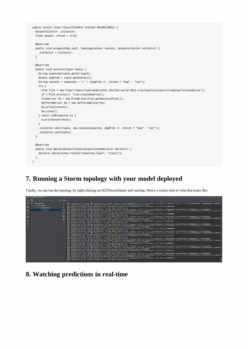
public static class ClassifierBolt extends BaseRichBolt {
OutputCollector _collector;
final double _thresh = 0.54;
@Override
public void prepare(Map conf, TopologyContext context, OutputCollector collector) {
_collector = collector;
}
@Override
public void execute(Tuple tuple) {
String expected=tuple.getString(0);
double dogProb = tuple.getDouble(1);
String content = expected + "," + (dogProb <= _thresh ? "dog" : "cat");
try {
File file = new File("/Users/ludirehak/other_h2o/h2o-world-2015-training/tutorials/streaming/storm/web/out");
if (!file.exists()) file.createNewFile();
FileWriter fw = new FileWriter(file.getAbsoluteFile());
BufferedWriter bw = new BufferedWriter(fw);
bw.write(content);
bw.close();
} catch (IOException e) {
e.printStackTrace();
}
_collector.emit(tuple, new Values(expected, dogProb <= _thresh ? "dog" : "cat"));
_collector.ack(tuple);
}
@Override
public void declareOutputFields(OutputFieldsDeclarer declarer) {
declarer.declare(new Fields("expected_class", "class"));
}
}
7. Running a Storm topology with your model deployedFinally, we can run the topology by right-clicking on H2OStormStarter and running. Here's a screen shot of what that looks like:
8. Watching predictions in real-time

To watch the predictions in real time, we start up an http-server on port 4040 and navigate to http://localhost:4040.
In order to get http-server, install npm (you may need sudo):
brew install npm
npm install http-server -g
Once these are installed, you may navigate to the web directory and start the server:
cd web
http-server -p 4040 -c-1
Now open up your browser and navigate to http://localhost:4040. Requires a modern browser (depends on D3 for animation).
Here's a short video showing what it looks like all together.
Enjoy!
ReferencesCRANGBM
The Elements of Statistical Learning. Vol.1. N.p., page 339Hastie, Trevor, Robert Tibshirani, and J Jerome H Friedman.Springer New York, 2001.
Data Science with H2O (GBM)
Gradient Boosting (Wikipedia)
H2O
H2O Markov stable releaseJava POJORStorm
H2OWorld - Building Machine Learning Applications withSparkling Water
RequirementsOracle Java 7+ (USB)Spark 1.5.1 (USB)Sparkling Water 1.5.6 (USB)SMS dataset (USB)
Provided on USBBinariesSMS datasetSlidesScala Script
Machine Learning WorkflowGoal: For a given text message, identify if it is spam or not.
1. Extract data2. Transform & tokenize messages3. Build Spark's Tf-IDF model and expand messages to feature vectors4. Create and evaluate H2O's Deep Learning model5. Use the models to detect spam messages
Prepare environment
1. Run Sparkling shell with an embedded Spark cluster:
cd "path/to/sparkling/water"
export SPARK_HOME="/path/to/spark/installation"
export MASTER="local-cluster[3,2,4096]"
bin/sparkling-shell --conf spark.executor.memory=2G
Note: To avoid flooding output with Spark INFO messages, I recommend editing your $SPARK_HOME/conf/log4j.properties and configuring the log level to WARN .
2. Open Spark UI: Go to http://localhost:4040/ to see the Spark status.
3. Prepare the environment:
// Input data
val DATAFILE="../data/smsData.txt"
// Common imports from H2O and Sparks
import _root_.hex.deeplearning.{DeepLearningModel, DeepLearning}
import _root_.hex.deeplearning.DeepLearningParameters
import org.apache.spark.examples.h2o.DemoUtils._
import org.apache.spark.h2o._
import org.apache.spark.mllib
import org.apache.spark.mllib.feature.{IDFModel, IDF, HashingTF}
import org.apache.spark.rdd.RDD
import water.Key
4. Define the representation of the training message:
// Representation of a training message
case class SMS(target: String, fv: mllib.linalg.Vector)
5. Define the data loader and parser:
def load(dataFile: String): RDD[Array[String]] = {
// Load file into memory, split on TABs and filter all empty lines
sc.textFile(dataFile).map(l => l.split("\t")).filter(r => !r(0).isEmpty)
}
6. Define the input messages tokenizer:
// Tokenizer
// For each sentence in input RDD it provides array of string representing individual interesting words in the sentence
def tokenize(dataRDD: RDD[String]): RDD[Seq[String]] = {
// Ignore all useless words
val ignoredWords = Seq("the", "a", "", "in", "on", "at", "as", "not", "for")
// Ignore all useless characters
val ignoredChars = Seq(',', ':', ';', '/', '<', '>', '"', '.', '(', ')', '?', '-', '\'','!','0', '1')
// Invoke RDD API and transform input data
val textsRDD = dataRDD.map( r => {
// Get rid of all useless characters
var smsText = r.toLowerCase
for( c <- ignoredChars) {
smsText = smsText.replace(c, ' ')
}
// Remove empty and uninteresting words
val words = smsText.split(" ").filter(w => !ignoredWords.contains(w) && w.length>2).distinct
words.toSeq
})
textsRDD
}
7. Configure Spark's Tf-IDF model builder:
def buildIDFModel(tokensRDD: RDD[Seq[String]],
minDocFreq:Int = 4,
hashSpaceSize:Int = 1 << 10): (HashingTF, IDFModel, RDD[mllib.linalg.Vector]) = {
// Hash strings into the given space
val hashingTF = new HashingTF(hashSpaceSize)
val tf = hashingTF.transform(tokensRDD)
// Build term frequency-inverse document frequency model
val idfModel = new IDF(minDocFreq = minDocFreq).fit(tf)
val expandedTextRDD = idfModel.transform(tf)
(hashingTF, idfModel, expandedTextRDD)
}
Wikipedia defines TF-IDF as: "tf–idf, short for term frequency–inverse document frequency, is a numerical statistic that isintended to reflect how important a word is to a document in a collection or corpus. It is often used as a weighting factor ininformation retrieval and text mining. The tf-idf value increases proportionally to the number of times a word appears in thedocument, but is offset by the frequency of the word in the corpus, which helps to adjust for the fact that some words appearmore frequently in general."
8. Configure H2O's DeepLearning model builder:
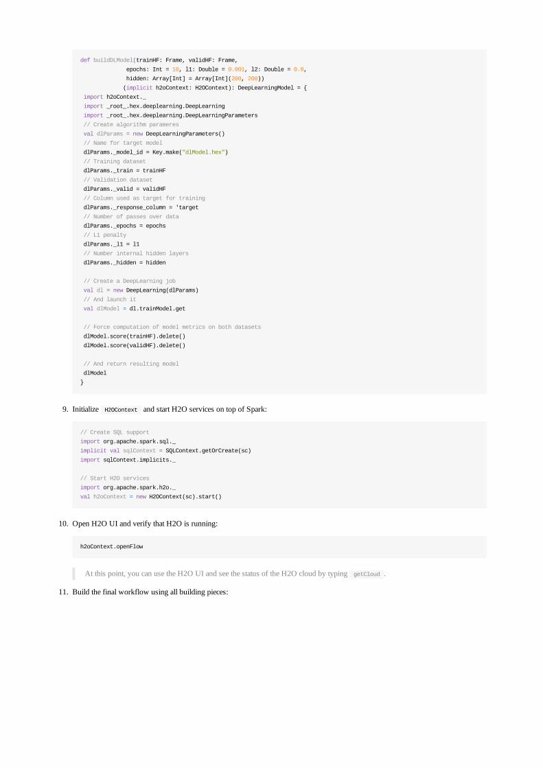
def buildDLModel(trainHF: Frame, validHF: Frame,
epochs: Int = 10, l1: Double = 0.001, l2: Double = 0.0,
hidden: Array[Int] = Array[Int](200, 200))
(implicit h2oContext: H2OContext): DeepLearningModel = {
import h2oContext._
import _root_.hex.deeplearning.DeepLearning
import _root_.hex.deeplearning.DeepLearningParameters
// Create algorithm parameres
val dlParams = new DeepLearningParameters()
// Name for target model
dlParams._model_id = Key.make("dlModel.hex")
// Training dataset
dlParams._train = trainHF
// Validation dataset
dlParams._valid = validHF
// Column used as target for training
dlParams._response_column = 'target
// Number of passes over data
dlParams._epochs = epochs
// L1 penalty
dlParams._l1 = l1
// Number internal hidden layers
dlParams._hidden = hidden
// Create a DeepLearning job
val dl = new DeepLearning(dlParams)
// And launch it
val dlModel = dl.trainModel.get
// Force computation of model metrics on both datasets
dlModel.score(trainHF).delete()
dlModel.score(validHF).delete()
// And return resulting model
dlModel
}
9. Initialize H2OContext and start H2O services on top of Spark:
// Create SQL support
import org.apache.spark.sql._
implicit val sqlContext = SQLContext.getOrCreate(sc)
import sqlContext.implicits._
// Start H2O services
import org.apache.spark.h2o._
val h2oContext = new H2OContext(sc).start()
10. Open H2O UI and verify that H2O is running:
h2oContext.openFlow
At this point, you can use the H2O UI and see the status of the H2O cloud by typing getCloud .
11. Build the final workflow using all building pieces:
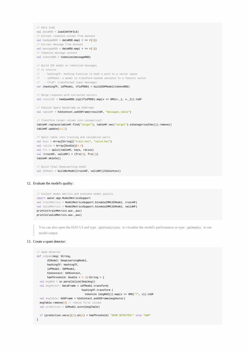
// Data load
val dataRDD = load(DATAFILE)
// Extract response column from dataset
val hamSpamRDD = dataRDD.map( r => r(0))
// Extract message from dataset
val messageRDD = dataRDD.map( r => r(1))
// Tokenize message content
val tokensRDD = tokenize(messageRDD)
// Build IDF model on tokenized messages
// It returns
// - hashingTF: hashing function to hash a word to a vector space
// - idfModel: a model to transform hashed sentence to a feature vector
// - tfidf: transformed input messages
var (hashingTF, idfModel, tfidfRDD) = buildIDFModel(tokensRDD)
// Merge response with extracted vectors
val resultDF = hamSpamRDD.zip(tfidfRDD).map(v => SMS(v._1, v._2)).toDF
// Publish Spark DataFrame as H2OFrame
val tableHF = h2oContext.asH2OFrame(resultDF, "messages_table")
// Transform target column into categorical!
tableHF.replace(tableHF.find("target"), tableHF.vec("target").toCategoricalVec()).remove()
tableHF.update(null)
// Split table into training and validation parts
val keys = Array[String]("train.hex", "valid.hex")
val ratios = Array[Double](0.8)
val frs = split(tableHF, keys, ratios)
val (trainHF, validHF) = (frs(0), frs(1))
tableHF.delete()
// Build final DeepLearning model
val dlModel = buildDLModel(trainHF, validHF)(h2oContext)
12. Evaluate the model's quality:
// Collect model metrics and evaluate model quality
import water.app.ModelMetricsSupport
val trainMetrics = ModelMetricsSupport.binomialMM(dlModel, trainHF)
val validMetrics = ModelMetricsSupport.binomialMM(dlModel, validHF)
println(trainMetrics.auc._auc)
println(validMetrics.auc._auc)
You can also open the H2O UI and type getPredictions to visualize the model's performance or type getModels to seemodel output.
13. Create a spam detector:
// Spam detector
def isSpam(msg: String,
dlModel: DeepLearningModel,
hashingTF: HashingTF,
idfModel: IDFModel,
h2oContext: H2OContext,
hamThreshold: Double = 0.5):String = {
val msgRdd = sc.parallelize(Seq(msg))
val msgVector: DataFrame = idfModel.transform(
hashingTF.transform (
tokenize (msgRdd))).map(v => SMS("?", v)).toDF
val msgTable: H2OFrame = h2oContext.asH2OFrame(msgVector)
msgTable.remove(0) // remove first column
val prediction = dlModel.score(msgTable)
if (prediction.vecs()(1).at(0) < hamThreshold) "SPAM DETECTED!" else "HAM"
}

14. Try to detect spam:
isSpam("Michal, h2oworld party tonight in MV?", dlModel, hashingTF, idfModel, h2oContext)
//
isSpam("We tried to contact you re your reply to our offer of a Video Handset? 750 anytime any networks mins? UNLIMITED TEXT?"
15. At this point, you have finished your 1st Sparkling Water Machine Learning application. Hack and enjoy! Thank you!
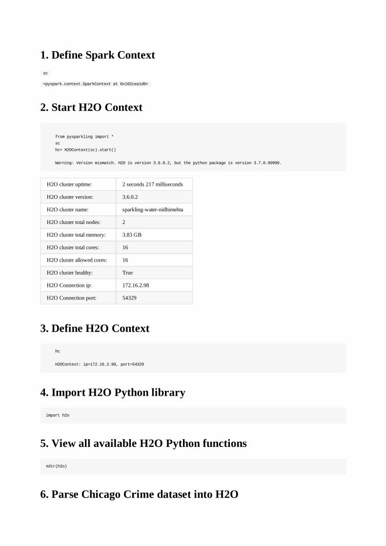
1. Define Spark Context sc
<pyspark.context.SparkContext at 0x102cea1d0>
2. Start H2O Context
from pysparkling import *
sc
hc= H2OContext(sc).start()
Warning: Version mismatch. H2O is version 3.6.0.2, but the python package is version 3.7.0.99999.
H2O cluster uptime: 2 seconds 217 milliseconds
H2O cluster version: 3.6.0.2
H2O cluster name: sparkling-water-nidhimehta
H2O cluster total nodes: 2
H2O cluster total memory: 3.83 GB
H2O cluster total cores: 16
H2O cluster allowed cores: 16
H2O cluster healthy: True
H2O Connection ip: 172.16.2.98
H2O Connection port: 54329
3. Define H2O Context
hc
H2OContext: ip=172.16.2.98, port=54329
4. Import H2O Python library
import h2o
5. View all available H2O Python functions
#dir(h2o)
6. Parse Chicago Crime dataset into H2O
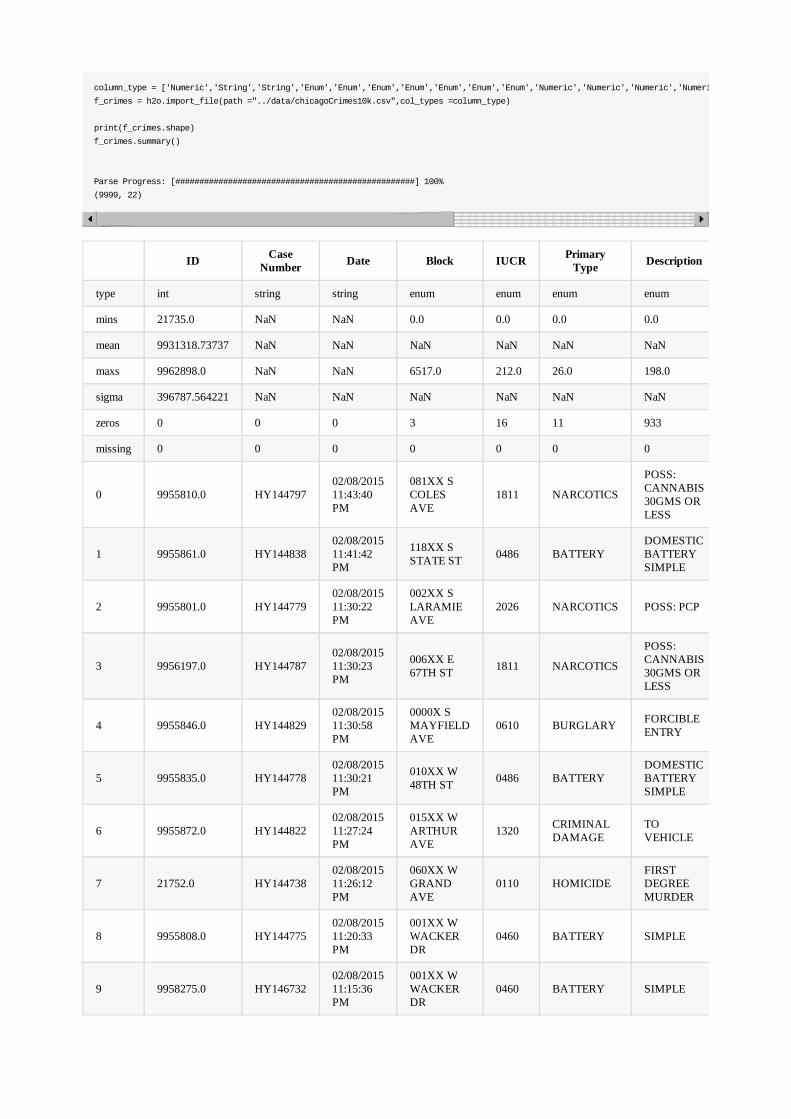
column_type = ['Numeric','String','String','Enum','Enum','Enum','Enum','Enum','Enum','Enum','Numeric','Numeric','Numeric','Numeric','Enum','Numeric','Numeric','Numeric','Enum','Numeric','Numeric','Enum']
f_crimes = h2o.import_file(path ="../data/chicagoCrimes10k.csv",col_types =column_type)
print(f_crimes.shape)
f_crimes.summary()
Parse Progress: [##################################################] 100%
(9999, 22)
ID CaseNumber Date Block IUCR Primary
Type Description
type int string string enum enum enum enum
mins 21735.0 NaN NaN 0.0 0.0 0.0 0.0
mean 9931318.73737 NaN NaN NaN NaN NaN NaN
maxs 9962898.0 NaN NaN 6517.0 212.0 26.0 198.0
sigma 396787.564221 NaN NaN NaN NaN NaN NaN
zeros 0 0 0 3 16 11 933
missing 0 0 0 0 0 0 0
0 9955810.0 HY14479702/08/201511:43:40PM
081XX SCOLESAVE
1811 NARCOTICS
POSS:CANNABIS30GMS ORLESS
1 9955861.0 HY14483802/08/201511:41:42PM
118XX SSTATE ST 0486 BATTERY
DOMESTICBATTERYSIMPLE
2 9955801.0 HY14477902/08/201511:30:22PM
002XX SLARAMIEAVE
2026 NARCOTICS POSS: PCP
3 9956197.0 HY14478702/08/201511:30:23PM
006XX E67TH ST 1811 NARCOTICS
POSS:CANNABIS30GMS ORLESS
4 9955846.0 HY14482902/08/201511:30:58PM
0000X SMAYFIELDAVE
0610 BURGLARY FORCIBLEENTRY
5 9955835.0 HY14477802/08/201511:30:21PM
010XX W48TH ST 0486 BATTERY
DOMESTICBATTERYSIMPLE
6 9955872.0 HY14482202/08/201511:27:24PM
015XX WARTHURAVE
1320 CRIMINALDAMAGE
TOVEHICLE
7 21752.0 HY14473802/08/201511:26:12PM
060XX WGRANDAVE
0110 HOMICIDEFIRSTDEGREEMURDER
8 9955808.0 HY14477502/08/201511:20:33PM
001XX WWACKERDR
0460 BATTERY SIMPLE
9 9958275.0 HY14673202/08/201511:15:36PM
001XX WWACKERDR
0460 BATTERY SIMPLE
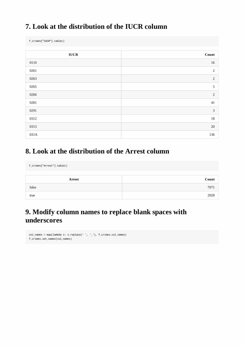
7. Look at the distribution of the IUCR column
f_crimes["IUCR"].table()
IUCR Count
0110 16
0261 2
0263 2
0265 5
0266 2
0281 41
0291 3
0312 18
0313 20
031A 136
8. Look at the distribution of the Arrest column
f_crimes["Arrest"].table()
Arrest Count
false 7071
true 2928
9. Modify column names to replace blank spaces withunderscores
col_names = map(lambda s: s.replace(' ', '_'), f_crimes.col_names)
f_crimes.set_names(col_names)
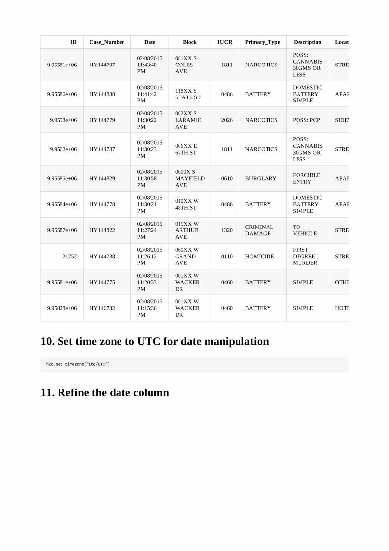
ID Case_Number Date Block IUCR Primary_Type Description Location_Description
9.95581e+06 HY14479702/08/201511:43:40PM
081XX SCOLESAVE
1811 NARCOTICS
POSS:CANNABIS30GMS ORLESS
STREET
9.95586e+06 HY14483802/08/201511:41:42PM
118XX SSTATE ST 0486 BATTERY
DOMESTICBATTERYSIMPLE
APARTMENT
9.9558e+06 HY14477902/08/201511:30:22PM
002XX SLARAMIEAVE
2026 NARCOTICS POSS: PCP SIDEWALK
9.9562e+06 HY14478702/08/201511:30:23PM
006XX E67TH ST 1811 NARCOTICS
POSS:CANNABIS30GMS ORLESS
STREET
9.95585e+06 HY14482902/08/201511:30:58PM
0000X SMAYFIELDAVE
0610 BURGLARY FORCIBLEENTRY APARTMENT
9.95584e+06 HY14477802/08/201511:30:21PM
010XX W48TH ST 0486 BATTERY
DOMESTICBATTERYSIMPLE
APARTMENT
9.95587e+06 HY14482202/08/201511:27:24PM
015XX WARTHURAVE
1320 CRIMINALDAMAGE
TOVEHICLE STREET
21752 HY14473802/08/201511:26:12PM
060XX WGRANDAVE
0110 HOMICIDEFIRSTDEGREEMURDER
STREET
9.95581e+06 HY14477502/08/201511:20:33PM
001XX WWACKERDR
0460 BATTERY SIMPLE OTHER
9.95828e+06 HY14673202/08/201511:15:36PM
001XX WWACKERDR
0460 BATTERY SIMPLE HOTEL/MOTEL
10. Set time zone to UTC for date manipulation
h2o.set_timezone("Etc/UTC")
11. Refine the date column
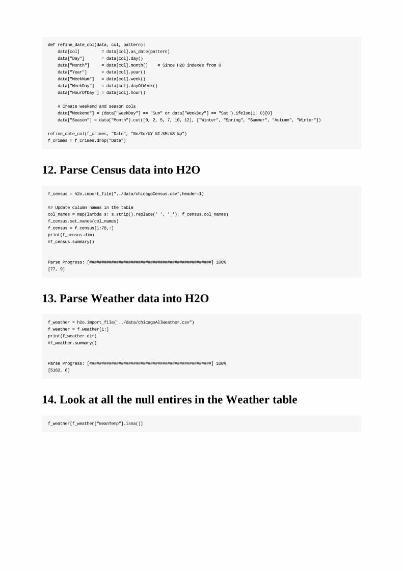
def refine_date_col(data, col, pattern):
data[col] = data[col].as_date(pattern)
data["Day"] = data[col].day()
data["Month"] = data[col].month() # Since H2O indexes from 0
data["Year"] = data[col].year()
data["WeekNum"] = data[col].week()
data["WeekDay"] = data[col].dayOfWeek()
data["HourOfDay"] = data[col].hour()
# Create weekend and season cols
data["Weekend"] = (data["WeekDay"] == "Sun" or data["WeekDay"] == "Sat").ifelse(1, 0)[0]
data["Season"] = data["Month"].cut([0, 2, 5, 7, 10, 12], ["Winter", "Spring", "Summer", "Autumn", "Winter"])
refine_date_col(f_crimes, "Date", "%m/%d/%Y %I:%M:%S %p")
f_crimes = f_crimes.drop("Date")
12. Parse Census data into H2O
f_census = h2o.import_file("../data/chicagoCensus.csv",header=1)
## Update column names in the table
col_names = map(lambda s: s.strip().replace(' ', '_'), f_census.col_names)
f_census.set_names(col_names)
f_census = f_census[1:78,:]
print(f_census.dim)
#f_census.summary()
Parse Progress: [##################################################] 100%
[77, 9]
13. Parse Weather data into H2O
f_weather = h2o.import_file("../data/chicagoAllWeather.csv")
f_weather = f_weather[1:]
print(f_weather.dim)
#f_weather.summary()
Parse Progress: [##################################################] 100%
[5162, 6]
14. Look at all the null entires in the Weather table
f_weather[f_weather["meanTemp"].isna()]
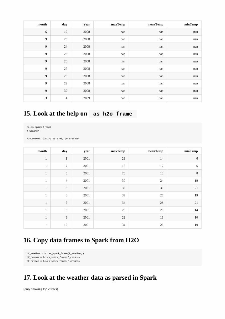
month day year maxTemp meanTemp minTemp
6 19 2008 nan nan nan
9 23 2008 nan nan nan
9 24 2008 nan nan nan
9 25 2008 nan nan nan
9 26 2008 nan nan nan
9 27 2008 nan nan nan
9 28 2008 nan nan nan
9 29 2008 nan nan nan
9 30 2008 nan nan nan
3 4 2009 nan nan nan
15. Look at the help on as_h2o_frame
hc.as_spark_frame?
f_weather
H2OContext: ip=172.16.2.98, port=54329
month day year maxTemp meanTemp minTemp
1 1 2001 23 14 6
1 2 2001 18 12 6
1 3 2001 28 18 8
1 4 2001 30 24 19
1 5 2001 36 30 21
1 6 2001 33 26 19
1 7 2001 34 28 21
1 8 2001 26 20 14
1 9 2001 23 16 10
1 10 2001 34 26 19
16. Copy data frames to Spark from H2O
df_weather = hc.as_spark_frame(f_weather,)
df_census = hc.as_spark_frame(f_census)
df_crimes = hc.as_spark_frame(f_crimes)
17. Look at the weather data as parsed in Spark(only showing top 2 rows)
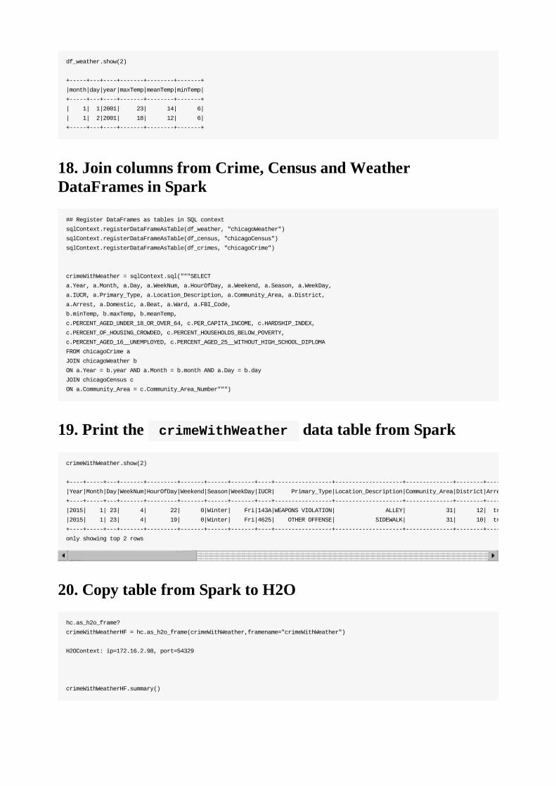
df_weather.show(2)
+-----+---+----+-------+--------+-------+
|month|day|year|maxTemp|meanTemp|minTemp|
+-----+---+----+-------+--------+-------+
| 1| 1|2001| 23| 14| 6|
| 1| 2|2001| 18| 12| 6|
+-----+---+----+-------+--------+-------+
18. Join columns from Crime, Census and WeatherDataFrames in Spark
## Register DataFrames as tables in SQL context
sqlContext.registerDataFrameAsTable(df_weather, "chicagoWeather")
sqlContext.registerDataFrameAsTable(df_census, "chicagoCensus")
sqlContext.registerDataFrameAsTable(df_crimes, "chicagoCrime")
crimeWithWeather = sqlContext.sql("""SELECT
a.Year, a.Month, a.Day, a.WeekNum, a.HourOfDay, a.Weekend, a.Season, a.WeekDay,
a.IUCR, a.Primary_Type, a.Location_Description, a.Community_Area, a.District,
a.Arrest, a.Domestic, a.Beat, a.Ward, a.FBI_Code,
b.minTemp, b.maxTemp, b.meanTemp,
c.PERCENT_AGED_UNDER_18_OR_OVER_64, c.PER_CAPITA_INCOME, c.HARDSHIP_INDEX,
c.PERCENT_OF_HOUSING_CROWDED, c.PERCENT_HOUSEHOLDS_BELOW_POVERTY,
c.PERCENT_AGED_16__UNEMPLOYED, c.PERCENT_AGED_25__WITHOUT_HIGH_SCHOOL_DIPLOMA
FROM chicagoCrime a
JOIN chicagoWeather b
ON a.Year = b.year AND a.Month = b.month AND a.Day = b.day
JOIN chicagoCensus c
ON a.Community_Area = c.Community_Area_Number""")
19. Print the crimeWithWeather data table from Spark
crimeWithWeather.show(2)
+----+-----+---+-------+---------+-------+------+-------+----+-----------------+--------------------+--------------+--------+------+--------+----+----+--------+-------+-------+--------+--------------------------------+-----------------+--------------+--------------------------+--------------------------------+---------------------------+--------------------------------------------+
|Year|Month|Day|WeekNum|HourOfDay|Weekend|Season|WeekDay|IUCR| Primary_Type|Location_Description|Community_Area|District|Arrest|Domestic|Beat|Ward|FBI_Code|minTemp|maxTemp|meanTemp|PERCENT_AGED_UNDER_18_OR_OVER_64|PER_CAPITA_INCOME|HARDSHIP_INDEX|PERCENT_OF_HOUSING_CROWDED|PERCENT_HOUSEHOLDS_BELOW_POVERTY|PERCENT_AGED_16__UNEMPLOYED|PERCENT_AGED_25__WITHOUT_HIGH_SCHOOL_DIPLOMA|
+----+-----+---+-------+---------+-------+------+-------+----+-----------------+--------------------+--------------+--------+------+--------+----+----+--------+-------+-------+--------+--------------------------------+-----------------+--------------+--------------------------+--------------------------------+---------------------------+--------------------------------------------+
|2015| 1| 23| 4| 22| 0|Winter| Fri|143A|WEAPONS VIOLATION| ALLEY| 31| 12| true| false|1234| 25| 15| 29| 31| 30| 32.6| 16444| 76| 9.600000000000001| 25.8| 15.8| 40.7|
|2015| 1| 23| 4| 19| 0|Winter| Fri|4625| OTHER OFFENSE| SIDEWALK| 31| 10| true| false|1034| 25| 26| 29| 31| 30| 32.6| 16444| 76| 9.600000000000001| 25.8| 15.8| 40.7|
+----+-----+---+-------+---------+-------+------+-------+----+-----------------+--------------------+--------------+--------+------+--------+----+----+--------+-------+-------+--------+--------------------------------+-----------------+--------------+--------------------------+--------------------------------+---------------------------+--------------------------------------------+
only showing top 2 rows
20. Copy table from Spark to H2O
hc.as_h2o_frame?
crimeWithWeatherHF = hc.as_h2o_frame(crimeWithWeather,framename="crimeWithWeather")
H2OContext: ip=172.16.2.98, port=54329
crimeWithWeatherHF.summary()
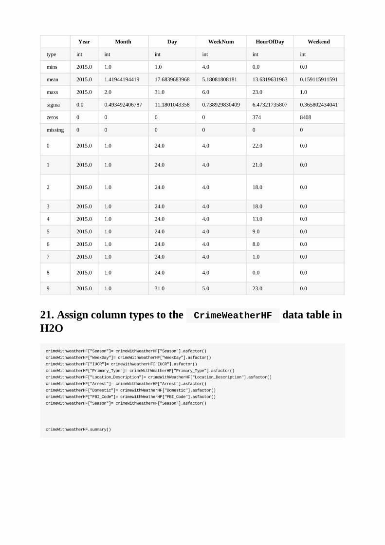
Year Month Day WeekNum HourOfDay Weekend
type int int int int int int
mins 2015.0 1.0 1.0 4.0 0.0 0.0
mean 2015.0 1.41944194419 17.6839683968 5.18081808181 13.6319631963 0.159115911591
maxs 2015.0 2.0 31.0 6.0 23.0 1.0
sigma 0.0 0.493492406787 11.1801043358 0.738929830409 6.47321735807 0.365802434041
zeros 0 0 0 0 374 8408
missing 0 0 0 0 0 0
0 2015.0 1.0 24.0 4.0 22.0 0.0
1 2015.0 1.0 24.0 4.0 21.0 0.0
2 2015.0 1.0 24.0 4.0 18.0 0.0
3 2015.0 1.0 24.0 4.0 18.0 0.0
4 2015.0 1.0 24.0 4.0 13.0 0.0
5 2015.0 1.0 24.0 4.0 9.0 0.0
6 2015.0 1.0 24.0 4.0 8.0 0.0
7 2015.0 1.0 24.0 4.0 1.0 0.0
8 2015.0 1.0 24.0 4.0 0.0 0.0
9 2015.0 1.0 31.0 5.0 23.0 0.0
21. Assign column types to the CrimeWeatherHF data table inH2O
crimeWithWeatherHF["Season"]= crimeWithWeatherHF["Season"].asfactor()
crimeWithWeatherHF["WeekDay"]= crimeWithWeatherHF["WeekDay"].asfactor()
crimeWithWeatherHF["IUCR"]= crimeWithWeatherHF["IUCR"].asfactor()
crimeWithWeatherHF["Primary_Type"]= crimeWithWeatherHF["Primary_Type"].asfactor()
crimeWithWeatherHF["Location_Description"]= crimeWithWeatherHF["Location_Description"].asfactor()
crimeWithWeatherHF["Arrest"]= crimeWithWeatherHF["Arrest"].asfactor()
crimeWithWeatherHF["Domestic"]= crimeWithWeatherHF["Domestic"].asfactor()
crimeWithWeatherHF["FBI_Code"]= crimeWithWeatherHF["FBI_Code"].asfactor()
crimeWithWeatherHF["Season"]= crimeWithWeatherHF["Season"].asfactor()
crimeWithWeatherHF.summary()
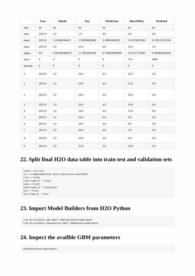
Year Month Day WeekNum HourOfDay Weekend
type int int int int int int
mins 2015.0 1.0 1.0 4.0 0.0 0.0
mean 2015.0 1.41944194419 17.6839683968 5.18081808181 13.6319631963 0.159115911591
maxs 2015.0 2.0 31.0 6.0 23.0 1.0
sigma 0.0 0.493492406787 11.1801043358 0.738929830409 6.47321735807 0.365802434041
zeros 0 0 0 0 374 8408
missing 0 0 0 0 0 0
0 2015.0 1.0 24.0 4.0 22.0 0.0
1 2015.0 1.0 24.0 4.0 21.0 0.0
2 2015.0 1.0 24.0 4.0 18.0 0.0
3 2015.0 1.0 24.0 4.0 18.0 0.0
4 2015.0 1.0 24.0 4.0 13.0 0.0
5 2015.0 1.0 24.0 4.0 9.0 0.0
6 2015.0 1.0 24.0 4.0 8.0 0.0
7 2015.0 1.0 24.0 4.0 1.0 0.0
8 2015.0 1.0 24.0 4.0 0.0 0.0
9 2015.0 1.0 31.0 5.0 23.0 0.0
22. Split final H2O data table into train test and validation sets
ratios = [0.6,0.2]
frs = crimeWithWeatherHF.split_frame(ratios,seed=12345)
train = frs[0]
train.frame_id = "Train"
valid = frs[2]
valid.frame_id = "Validation"
test = frs[1]
test.frame_id = "Test"
23. Import Model Builders from H2O Python
from h2o.estimators.gbm import H2OGradientBoostingEstimator
from h2o.estimators.deeplearning import H2ODeepLearningEstimator
24. Inspect the availble GBM parameters
H2OGradientBoostingEstimator?
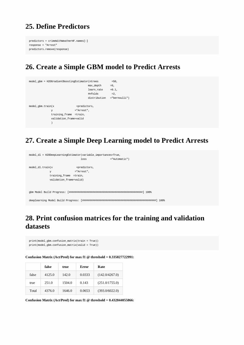
25. Define Predictors
predictors = crimeWithWeatherHF.names[:]
response = "Arrest"
predictors.remove(response)
26. Create a Simple GBM model to Predict Arrests
model_gbm = H2OGradientBoostingEstimator(ntrees =50,
max_depth =6,
learn_rate =0.1,
#nfolds =2,
distribution ="bernoulli")
model_gbm.train(x =predictors,
y ="Arrest",
training_frame =train,
validation_frame=valid
)
27. Create a Simple Deep Learning model to Predict Arrests
model_dl = H2ODeepLearningEstimator(variable_importances=True,
loss ="Automatic")
model_dl.train(x =predictors,
y ="Arrest",
training_frame =train,
validation_frame=valid)
gbm Model Build Progress: [##################################################] 100%
deeplearning Model Build Progress: [##################################################] 100%
28. Print confusion matrices for the training and validationdatasets
print(model_gbm.confusion_matrix(train = True))
print(model_gbm.confusion_matrix(valid = True))
Confusion Matrix (Act/Pred) for max f1 @ threshold = 0.335827722991:
false true Error Rate
false 4125.0 142.0 0.0333 (142.0/4267.0)
true 251.0 1504.0 0.143 (251.0/1755.0)
Total 4376.0 1646.0 0.0653 (393.0/6022.0)
Confusion Matrix (Act/Pred) for max f1 @ threshold = 0.432844055866:
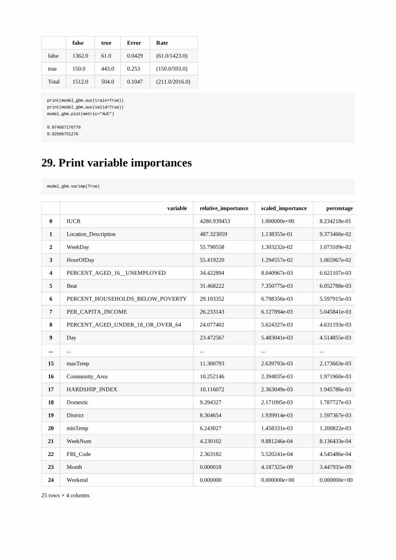
false true Error Rate
false 1362.0 61.0 0.0429 (61.0/1423.0)
true 150.0 443.0 0.253 (150.0/593.0)
Total 1512.0 504.0 0.1047 (211.0/2016.0)
print(model_gbm.auc(train=True))
print(model_gbm.auc(valid=True))
model_gbm.plot(metric="AUC")
0.974667176776
0.92596751276
29. Print variable importances
model_gbm.varimp(True)
variable relative_importance scaled_importance percentage
0 IUCR 4280.939453 1.000000e+00 8.234218e-01
1 Location_Description 487.323059 1.138355e-01 9.373466e-02
2 WeekDay 55.790558 1.303232e-02 1.073109e-02
3 HourOfDay 55.419220 1.294557e-02 1.065967e-02
4 PERCENT_AGED_16__UNEMPLOYED 34.422894 8.040967e-03 6.621107e-03
5 Beat 31.468222 7.350775e-03 6.052788e-03
6 PERCENT_HOUSEHOLDS_BELOW_POVERTY 29.103352 6.798356e-03 5.597915e-03
7 PER_CAPITA_INCOME 26.233143 6.127894e-03 5.045841e-03
8 PERCENT_AGED_UNDER_18_OR_OVER_64 24.077402 5.624327e-03 4.631193e-03
9 Day 23.472567 5.483041e-03 4.514855e-03
... ... ... ... ...
15 maxTemp 11.300793 2.639793e-03 2.173663e-03
16 Community_Area 10.252146 2.394835e-03 1.971960e-03
17 HARDSHIP_INDEX 10.116072 2.363049e-03 1.945786e-03
18 Domestic 9.294327 2.171095e-03 1.787727e-03
19 District 8.304654 1.939914e-03 1.597367e-03
20 minTemp 6.243027 1.458331e-03 1.200822e-03
21 WeekNum 4.230102 9.881246e-04 8.136433e-04
22 FBI_Code 2.363182 5.520241e-04 4.545486e-04
23 Month 0.000018 4.187325e-09 3.447935e-09
24 Weekend 0.000000 0.000000e+00 0.000000e+00
25 rows × 4 columns
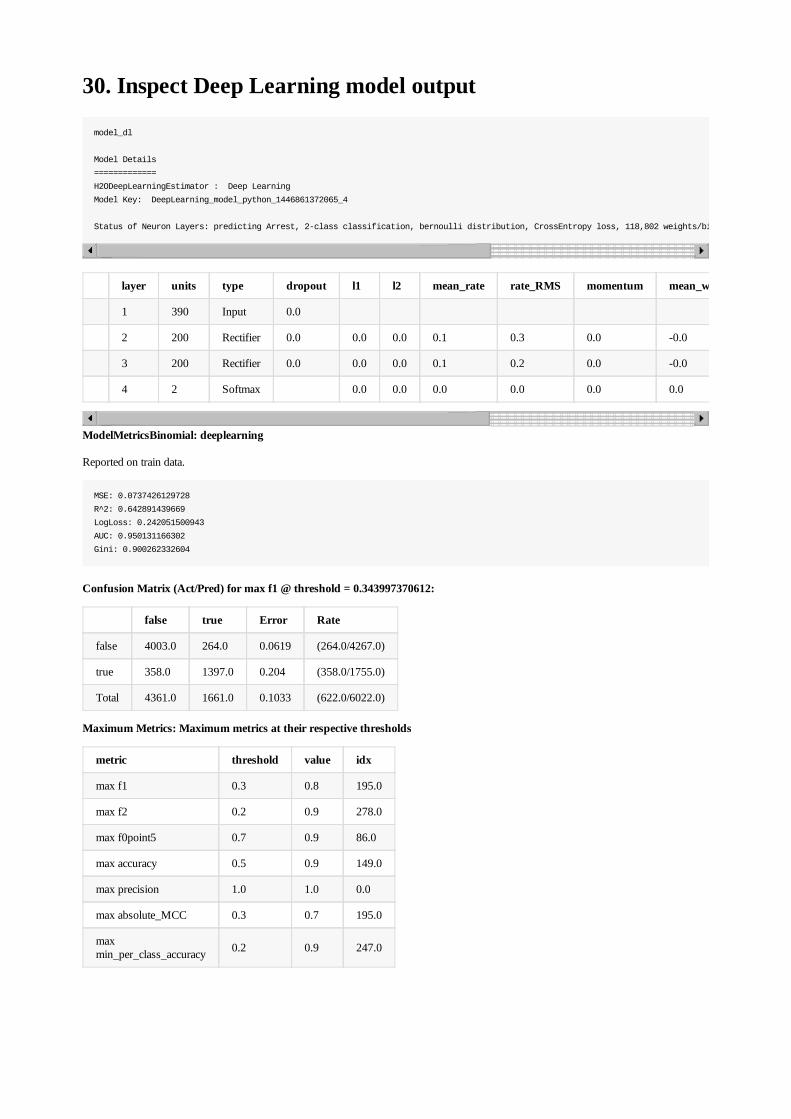
30. Inspect Deep Learning model output
model_dl
Model Details
=============
H2ODeepLearningEstimator : Deep Learning
Model Key: DeepLearning_model_python_1446861372065_4
Status of Neuron Layers: predicting Arrest, 2-class classification, bernoulli distribution, CrossEntropy loss, 118,802 weights/biases, 1.4 MB, 72,478 training samples, mini-batch size 1
layer units type dropout l1 l2 mean_rate rate_RMS momentum mean_weight
1 390 Input 0.0
2 200 Rectifier 0.0 0.0 0.0 0.1 0.3 0.0 -0.0
3 200 Rectifier 0.0 0.0 0.0 0.1 0.2 0.0 -0.0
4 2 Softmax 0.0 0.0 0.0 0.0 0.0 0.0
ModelMetricsBinomial: deeplearning
Reported on train data.
MSE: 0.0737426129728
R^2: 0.642891439669
LogLoss: 0.242051500943
AUC: 0.950131166302
Gini: 0.900262332604
Confusion Matrix (Act/Pred) for max f1 @ threshold = 0.343997370612:
false true Error Rate
false 4003.0 264.0 0.0619 (264.0/4267.0)
true 358.0 1397.0 0.204 (358.0/1755.0)
Total 4361.0 1661.0 0.1033 (622.0/6022.0)
Maximum Metrics: Maximum metrics at their respective thresholds
metric threshold value idx
max f1 0.3 0.8 195.0
max f2 0.2 0.9 278.0
max f0point5 0.7 0.9 86.0
max accuracy 0.5 0.9 149.0
max precision 1.0 1.0 0.0
max absolute_MCC 0.3 0.7 195.0
maxmin_per_class_accuracy 0.2 0.9 247.0
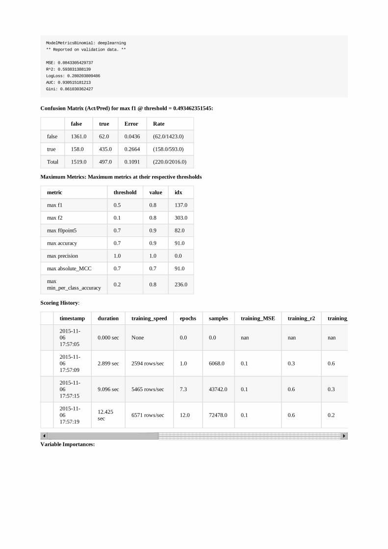
ModelMetricsBinomial: deeplearning
** Reported on validation data. **
MSE: 0.0843305429737
R^2: 0.593831388139
LogLoss: 0.280203809486
AUC: 0.930515181213
Gini: 0.861030362427
Confusion Matrix (Act/Pred) for max f1 @ threshold = 0.493462351545:
false true Error Rate
false 1361.0 62.0 0.0436 (62.0/1423.0)
true 158.0 435.0 0.2664 (158.0/593.0)
Total 1519.0 497.0 0.1091 (220.0/2016.0)
Maximum Metrics: Maximum metrics at their respective thresholds
metric threshold value idx
max f1 0.5 0.8 137.0
max f2 0.1 0.8 303.0
max f0point5 0.7 0.9 82.0
max accuracy 0.7 0.9 91.0
max precision 1.0 1.0 0.0
max absolute_MCC 0.7 0.7 91.0
maxmin_per_class_accuracy 0.2 0.8 236.0
Scoring History:
timestamp duration training_speed epochs samples training_MSE training_r2 training_logloss
2015-11-0617:57:05
0.000 sec None 0.0 0.0 nan nan nan
2015-11-0617:57:09
2.899 sec 2594 rows/sec 1.0 6068.0 0.1 0.3 0.6
2015-11-0617:57:15
9.096 sec 5465 rows/sec 7.3 43742.0 0.1 0.6 0.3
2015-11-0617:57:19
12.425sec 6571 rows/sec 12.0 72478.0 0.1 0.6 0.2
Variable Importances:
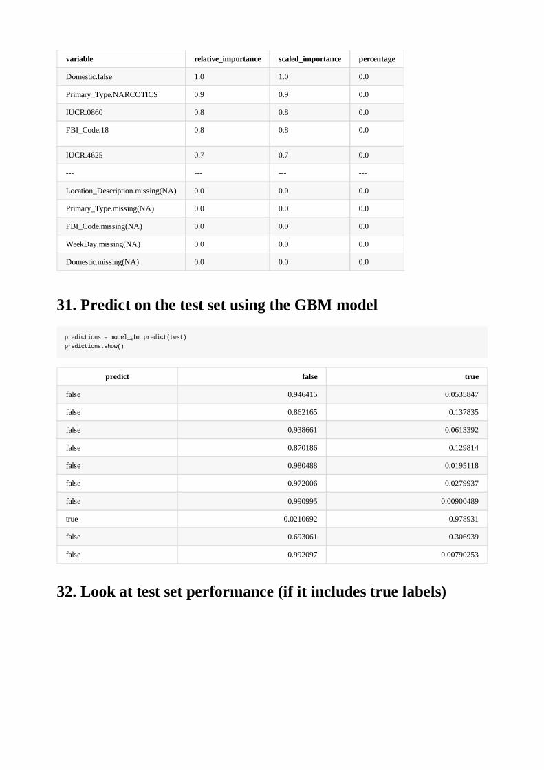
variable relative_importance scaled_importance percentage
Domestic.false 1.0 1.0 0.0
Primary_Type.NARCOTICS 0.9 0.9 0.0
IUCR.0860 0.8 0.8 0.0
FBI_Code.18 0.8 0.8 0.0
IUCR.4625 0.7 0.7 0.0
--- --- --- ---
Location_Description.missing(NA) 0.0 0.0 0.0
Primary_Type.missing(NA) 0.0 0.0 0.0
FBI_Code.missing(NA) 0.0 0.0 0.0
WeekDay.missing(NA) 0.0 0.0 0.0
Domestic.missing(NA) 0.0 0.0 0.0
31. Predict on the test set using the GBM model
predictions = model_gbm.predict(test)
predictions.show()
predict false true
false 0.946415 0.0535847
false 0.862165 0.137835
false 0.938661 0.0613392
false 0.870186 0.129814
false 0.980488 0.0195118
false 0.972006 0.0279937
false 0.990995 0.00900489
true 0.0210692 0.978931
false 0.693061 0.306939
false 0.992097 0.00790253
32. Look at test set performance (if it includes true labels)
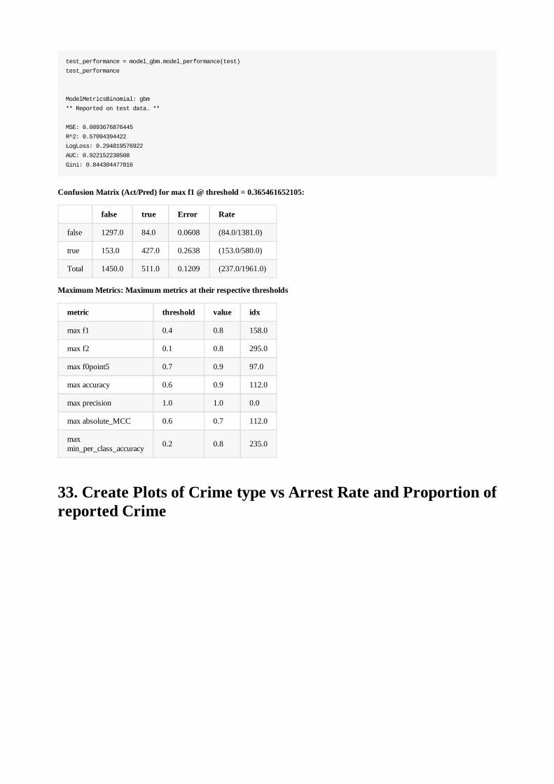
test_performance = model_gbm.model_performance(test)
test_performance
ModelMetricsBinomial: gbm
** Reported on test data. **
MSE: 0.0893676876445
R^2: 0.57094394422
LogLoss: 0.294019576922
AUC: 0.922152238508
Gini: 0.844304477016
Confusion Matrix (Act/Pred) for max f1 @ threshold = 0.365461652105:
false true Error Rate
false 1297.0 84.0 0.0608 (84.0/1381.0)
true 153.0 427.0 0.2638 (153.0/580.0)
Total 1450.0 511.0 0.1209 (237.0/1961.0)
Maximum Metrics: Maximum metrics at their respective thresholds
metric threshold value idx
max f1 0.4 0.8 158.0
max f2 0.1 0.8 295.0
max f0point5 0.7 0.9 97.0
max accuracy 0.6 0.9 112.0
max precision 1.0 1.0 0.0
max absolute_MCC 0.6 0.7 112.0
maxmin_per_class_accuracy 0.2 0.8 235.0
33. Create Plots of Crime type vs Arrest Rate and Proportion ofreported Crime
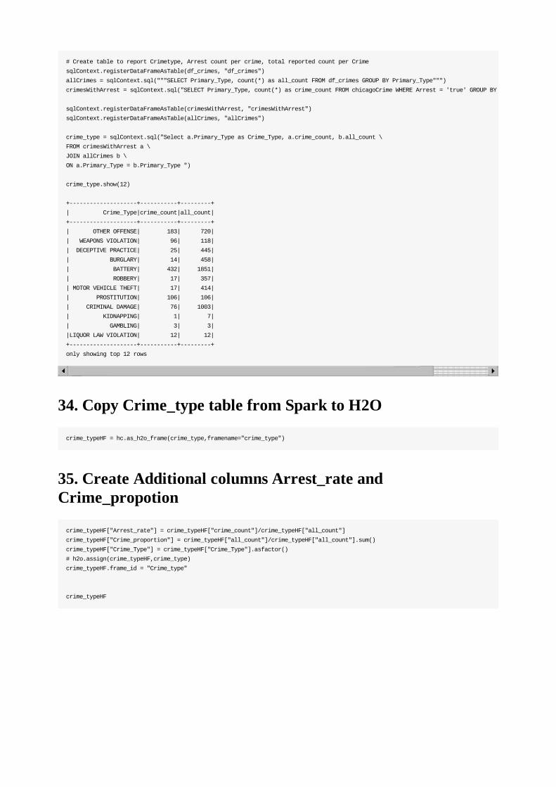
# Create table to report Crimetype, Arrest count per crime, total reported count per Crime
sqlContext.registerDataFrameAsTable(df_crimes, "df_crimes")
allCrimes = sqlContext.sql("""SELECT Primary_Type, count(*) as all_count FROM df_crimes GROUP BY Primary_Type""")
crimesWithArrest = sqlContext.sql("SELECT Primary_Type, count(*) as crime_count FROM chicagoCrime WHERE Arrest = 'true' GROUP BY Primary_Type")
sqlContext.registerDataFrameAsTable(crimesWithArrest, "crimesWithArrest")
sqlContext.registerDataFrameAsTable(allCrimes, "allCrimes")
crime_type = sqlContext.sql("Select a.Primary_Type as Crime_Type, a.crime_count, b.all_count \
FROM crimesWithArrest a \
JOIN allCrimes b \
ON a.Primary_Type = b.Primary_Type ")
crime_type.show(12)
+--------------------+-----------+---------+
| Crime_Type|crime_count|all_count|
+--------------------+-----------+---------+
| OTHER OFFENSE| 183| 720|
| WEAPONS VIOLATION| 96| 118|
| DECEPTIVE PRACTICE| 25| 445|
| BURGLARY| 14| 458|
| BATTERY| 432| 1851|
| ROBBERY| 17| 357|
| MOTOR VEHICLE THEFT| 17| 414|
| PROSTITUTION| 106| 106|
| CRIMINAL DAMAGE| 76| 1003|
| KIDNAPPING| 1| 7|
| GAMBLING| 3| 3|
|LIQUOR LAW VIOLATION| 12| 12|
+--------------------+-----------+---------+
only showing top 12 rows
34. Copy Crime_type table from Spark to H2O
crime_typeHF = hc.as_h2o_frame(crime_type,framename="crime_type")
35. Create Additional columns Arrest_rate andCrime_propotion
crime_typeHF["Arrest_rate"] = crime_typeHF["crime_count"]/crime_typeHF["all_count"]
crime_typeHF["Crime_proportion"] = crime_typeHF["all_count"]/crime_typeHF["all_count"].sum()
crime_typeHF["Crime_Type"] = crime_typeHF["Crime_Type"].asfactor()
# h2o.assign(crime_typeHF,crime_type)
crime_typeHF.frame_id = "Crime_type"
crime_typeHF
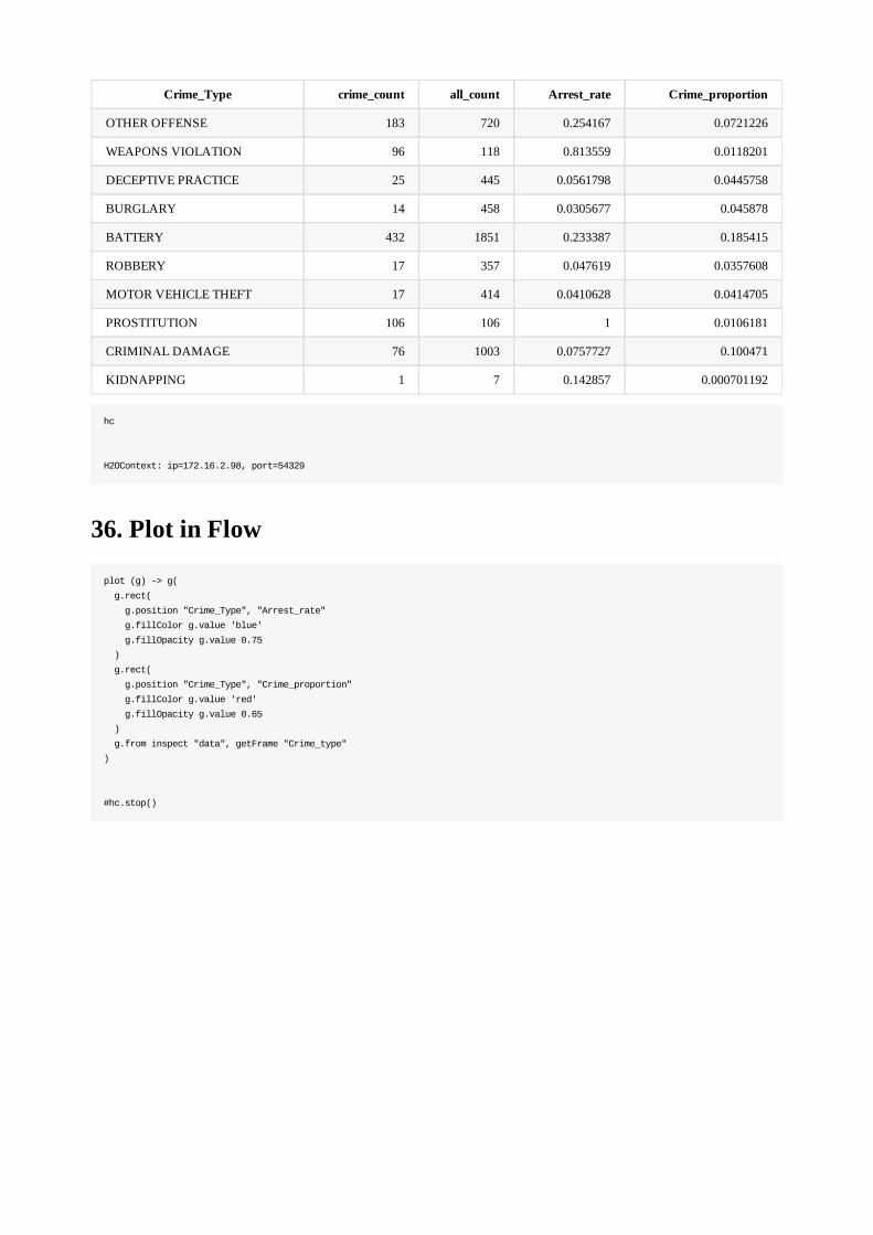
Crime_Type crime_count all_count Arrest_rate Crime_proportion
OTHER OFFENSE 183 720 0.254167 0.0721226
WEAPONS VIOLATION 96 118 0.813559 0.0118201
DECEPTIVE PRACTICE 25 445 0.0561798 0.0445758
BURGLARY 14 458 0.0305677 0.045878
BATTERY 432 1851 0.233387 0.185415
ROBBERY 17 357 0.047619 0.0357608
MOTOR VEHICLE THEFT 17 414 0.0410628 0.0414705
PROSTITUTION 106 106 1 0.0106181
CRIMINAL DAMAGE 76 1003 0.0757727 0.100471
KIDNAPPING 1 7 0.142857 0.000701192
hc
H2OContext: ip=172.16.2.98, port=54329
36. Plot in Flow
plot (g) -> g(
g.rect(
g.position "Crime_Type", "Arrest_rate"
g.fillColor g.value 'blue'
g.fillOpacity g.value 0.75
)
g.rect(
g.position "Crime_Type", "Crime_proportion"
g.fillColor g.value 'red'
g.fillOpacity g.value 0.65
)
g.from inspect "data", getFrame "Crime_type"
)
#hc.stop()
ResourcesMore information about machine learning with H2O
H2ODocumentation for H2O and Sparkling Water: http://docs.h2o.ai/
Glossary of terms: https://github.com/h2oai/h2o-3/blob/master/h2o-docs/src/product/tutorials/glossary.md
Open forum for questions about H2O (Google account required): https://groups.google.com/forum/#!forum/h2ostream
Track or file bug reports for H2O: https://jira.h2o.ai
GitHub repository for H2O: https://github.com/h2oai
PythonAbout Python: https://www.python.org/
Latest Python H2O documentation: http://h2o-release.s3.amazonaws.com/h2o/latest_stable_Pydoc.html
RAbout R: https://www.r-project.org/about.html
Download R: https://cran.r-project.org/mirrors.html
Latest R API H2O documentation: http://h2o-release.s3.amazonaws.com/h2o/latest_stable_Rdoc.html
Sparkling WaterAbout Spark: http://spark.apache.org/
Download Spark: http://spark.apache.org/downloads.html
Sparkling Water Developer documentation: https://github.com/h2oai/sparkling-water/blob/master/doc/devel/devel.rst


![Central Metabolism Cofactor Biosynthesis · ppp9 pi h h2o ppi h h2o h2o dad-5 h[p] atp adp h pi h2o succoa lipoate atp glx 2p4c2me xu5p-D h2o cbl1 ppi h[e] h2o h dad-5 gthrd asp-L](https://img.dokumen.tips/doc/110x75/5f47678d7025ea6bb340bf3d/central-metabolism-cofactor-biosynthesis-ppp9-pi-h-h2o-ppi-h-h2o-h2o-dad-5-hp.jpg)