Grobner Bases: Computational AlgebraicGeometry and its Complexity

Johannes Mittmann

Technische Universitat Munchen

May 9, 2007

Abstract

This paper gives an introduction to computational commutative al-gebra. Besides classical algebraic geometry and Grobner basis theory,we will discuss the computational complexity of some decision problemsinvolved.

Contents

1 Introduction 2

2 Algebraic Geometry 22.1 Ideals . . . . . . . . . . . . . . . . . . . . . . . . . . . . . . . . 22.2 Affine Varieties . . . . . . . . . . . . . . . . . . . . . . . . . . . 52.3 Hilbert’s Nullstellensatz . . . . . . . . . . . . . . . . . . . . . . 62.4 Algebra–Geometry Dictionary . . . . . . . . . . . . . . . . . . . 9

3 Grobner Bases 93.1 Division Algorithm . . . . . . . . . . . . . . . . . . . . . . . . . 103.2 Existence and Uniqueness . . . . . . . . . . . . . . . . . . . . . 133.3 Buchberger’s Algorithm . . . . . . . . . . . . . . . . . . . . . . 153.4 Applications . . . . . . . . . . . . . . . . . . . . . . . . . . . . . 17

4 Computational Complexity 184.1 Degree Bounds . . . . . . . . . . . . . . . . . . . . . . . . . . . 194.2 Mayr–Meyer Ideals . . . . . . . . . . . . . . . . . . . . . . . . . 20

1

1 Introduction

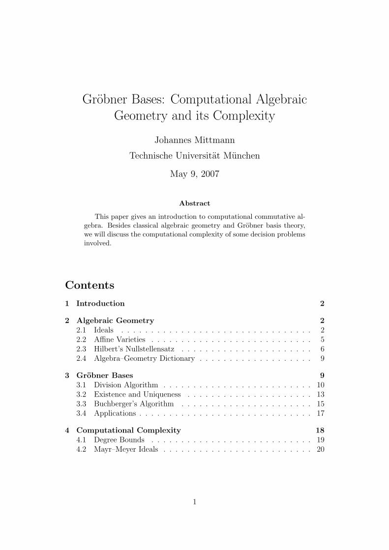
Problems from many different areas lead to a system of multivariate polynomialequations. Among them are robotics, term rewriting or automatic theoremproving in geometry. We give a simple example from graph theory.

Example. We want to find a 3-colouring of the following graph G = (V, E):

1

2

3

4

If we take as colours the three cubic roots of unity 1, e(2/3)πi, e(4/3)πi, the 3-colourings of G are exactly the tuples (ξ1, . . . , ξ4) ∈ C4 satisfying

X3i − 1 = 0, for all vertices i ∈ V ,

X2i + XiXj + X2

j = 0, for all edges (i, j) ∈ E.

2 Algebraic Geometry

Classical algebraic geometry studies zero sets of systems of polynomial equa-tions. This section follows parts of a lecture on commutative algebra given byProf. Gregor Kemper at the Technische Universitat Munchen in 2006. Furtherreferences are [CLO97] and [La05].

In this paper, R is always a commutative ring with unity, and K is alwaysa field. By N we denote the natural numbers N = {0, 1, 2, . . . }.

2.1 Ideals

Our main algebraic object of interest will be the ideal in a ring.

Definition 1. A subset I ⊆ R is called an ideal in R, written I E R, if

(i) 0 ∈ I,

(ii) a + b ∈ I for all a, b ∈ I, and

(iii) r · a ∈ I for all r ∈ R and a ∈ I.

Ideals are exactly the kernels of ring homomorphisms. In ring theory, theyplay a similar role as for example normal subgroups in group theory. Thefollowing property of ideals is immediate.

2

Proposition 2. Let M be a nonempty set of ideals in R. Then⋂I∈M

I

is an ideal in R.

Ideals can be described by means of generating sets.

Definition 3. Let A ⊆ R be a subset. Then

〈A〉 =⋂

IER, A⊆I

I

is called the ideal generated by A.

Hence, 〈A〉 is the smallest ideal containing A. For algorithmic purposes,finite generating sets are of particular interest. In this case, every element ofthe ideal can be written as an R-linear combination of the generators.

Definition 4. An ideal I E R is called finitely generated if there exist a1, . . . , as ∈R such that

I = 〈a1, . . . , as〉.

Proposition 5. Let a1, . . . , as ∈ R. Then

〈a1, . . . , as〉 ={∑s

i=1 riai | r1, . . . , rs ∈ R}.

The basic operations that can be performed with ideals are the following.

Definition 6. Let I, J E R be ideals.

(1) The sum of I and J is defined by

I + J ={a + b | a ∈ I and b ∈ J

}E R.

(2) The product of I and J is defined by

I · J ={∑s

i=1 aibi | ai ∈ I, bi ∈ J and s ∈ N>0

}E R.

I +J is the smallest ideal containing both I and J . Given the generators offinitely generated ideals it is easy to find generators for the sum and product.For the intersection this is not evident a priori.

Proposition 7. Let I = 〈a1, . . . , as〉 E R and J = 〈b1, . . . , bt〉 E R be ideals.Then:

(1) I + J = 〈a1, . . . , as, b1, . . . , bt〉.

(2) I · J = 〈aibj | 1 ≤ i ≤ s and 1 ≤ j ≤ t〉.

3

Rings in which every ideal is finitely generated are called Noetherian andcan be characterized as follows.

Definition 8. A ring R is called Noetherian if it satisfies the ascending chaincondition (ACC): Let I1, I2, I3, . . . E R be ideals with

I1 ⊆ I2 ⊆ I3 ⊆ . . . ,

then there exits an N ∈ N>0 such that IN = IN+1 = IN+2 = . . . .

Proposition 9. Let R be a ring. Then the following are equivalent:

(1) R is Noetherian.

(2) Every ideal I E R is finitely generated.

(3) Every nonempty set M of ideals in R has a maximal element.

Proof. (2) ⇒ (1): Let I1, I2, I3, . . . E R be ideals with

I1 ⊆ I2 ⊆ I3 ⊆ . . . .

Then I :=⋃

i∈N>0Ii is an ideal in R. By (2), there are a1, . . . , as ∈ R such

that I = 〈a1, . . . , as〉. Hence, there is an N ∈ N>0 with a1, . . . , as ∈ IN andtherefore IN = IN+1 = . . . .

(1)⇒ (3): Assume by way of contradiction that there exists a nonempty setM of ideals in R that has no maximal member. We will use this to constructinductively an infinite proper ascending chain of ideals. SinceM 6= 0, we canchoose I1 ∈M. Suppose we have

I1 ( I2 ( · · · ( Ii

with I1, . . . , Ii ∈M for some i ≥ 1. Since Ii is not maximal inM, there existsan ideal Ii+1 ∈ M with Ii ( Ii+1. Continuing this process yields a chain asdesired contradicting (1).

(3) ⇒ (2): Let I E R. Define

M ={J E R | J finitely generated with J ⊆ I

}6= 0.

By (3), there is a maximal element I ′ ∈M. Suppose that I ′ ( I. Then thereis an a ∈ I \ I ′. Hence I ′ + 〈a〉 ⊆ I is finitely generated contradicting themaximality of I ′. Therefore I = I ′ is finitely generated.

As a consequence, principal ideal domains like Z or K[X] and fields K areNoetherian. A famous result due to Hilbert now shows that polynomial ringsover Noetherian rings are again Noetherian.

Theorem 10 (The Hilbert Basis Theorem). Let R be a Noetherian ring. Then

R[X] is Noetherian.

4

Proof. Let I E R[X]. We want to show that I is finitely generated. Fori = 1, 2, . . . define

Ii ={lc(f) | f ∈ I with deg(f) = i

}∪

{0}⊆ R.

It is easy to see that I1, I2, . . . E R and I1 ⊆ I2 ⊆ · · · . Since R is Noetherian,there is an N ∈ N>0 such that IN = IN+1 = . . . . Moreover, there is an s ∈ N>0

and ai1, . . . , ais ∈ Ii such that

Ii = 〈ai1, . . . , ais〉

for all i = 1, . . . , N . By the definition of the Ii, we can choose polynomialsfij ∈ I with deg(fij) = i or deg(fij) = −∞ such that aij = lc(fij) for alli = 1, . . . , N and j = 1, . . . , s. Define

I ′ := 〈fij | i = 1, . . . , N and j = 1, . . . , s〉 ⊆ I.

To finish the proof it suffices to show I ⊆ I ′. Let f ∈ I. We argue by inductionon i := deg(f) that f ∈ I ′. The statement is clear for f = 0. If i ≥ 0, denotek = min{i, N} and ` = max{i, N}. We can write lc(f) =

∑sj=1 rjakj for some

r1, . . . , rs ∈ R. Define

f ′ :=s∑

j=1

rjfkjX`−N ∈ I ′.

Then deg(f ′) = i = deg(f) and lc(f ′) = lc(f). Therefore deg(f − f ′) < iand by induction it follows that f − f ′ ∈ I ′, hence f ∈ I ′.

Using induction, it follows that every ideal in a multivariate polynomialring over a field is finitely generated.

Corollary 11. Every ideal I E K[X1, . . . , Xn] is finitely generated. Moreover,for any A ⊆ K[X1, . . . , Xn] there is a finite subset B ⊆ A such that

〈A〉 = 〈B〉.

2.2 Affine Varieties

Affine varieties are the common zero set of a system of polynomials and willbe considered as an geometric object in the affine space Kn.

Definition 12. Let I ⊆ K[X1, . . . , Xn] be a subset. Then the set

Var(I) ={(ξ1, . . . , ξn) ∈ Kn | f(ξ1, . . . , ξn) = 0 for all f ∈ I

}is called the affine variety defined by I.

By the following proposition, we can always assume our system of polyno-mials to be an ideal.

5

Proposition 13. Let f1, . . . , fs ∈ K[X1, . . . , Xn]. Then

Var(f1, . . . , fs) = Var(〈f1, . . . , fs〉

).

On the other hand, given a set of zeros in affine space, we can consider allpolynomials that vanish on all zeros simultaneously.

Definition 14. Let V ⊆ Kn be a subset. Then the set

Id(V ) ={f ∈ K[X1, . . . , Xn] | f(ξ1, . . . , ξn) = 0 for all (ξ1, . . . , ξn) ∈ V

}is called the (vanishing) ideal of V .

It is easy to verify that Id(V ) is indeed an ideal.

Proposition 15. Let V ⊆ Kn be a subset. Then

Id(V ) E K[X1, . . . , Xn].

The following proposition shows how operations on varieties correspond tooperations on ideals.

Proposition 16.

(1) We have ∅ = Var(K[X1, . . . , Xn]

)and Kn = Var

(〈0〉

).

(2) Let I, J E K[X1, . . . , Xn] be ideals. Then

Var(I) ∪ Var(J) = Var(I · J) = Var(I ∩ J).

(3) Let M be a nonempty set of ideals in K[X1, . . . , Xn]. Then⋂I∈M

Var(I) = Var(⋃

I∈M I).

In particular, affine varieties form the closed sets of a topology, which is calledthe Zariski topology on Kn.

2.3 Hilbert’s Nullstellensatz

In this section we derive a relationship between Var and Id. The result will bea generalization of the Fundamental Theorem of Algebra.

Theorem 17 (The Fundamental Theorem of Algebra). Every nonconstantpolynomial f ∈ C[X] has a root ξ ∈ C:

f(ξ) = 0.

6

Fields with this property are called algebraically closed. So let K be analgebraically closed field and I E K[X1, . . . , Xn] an ideal. Obviously Var(I) 6=0 can only hold if 1 /∈ I or equivalently I ( K[X1, . . . , Xn] is a proper ideal.It turns out that this condition is already sufficient.

Lemma 18. Let K be a field and let L/K be a field extension which is finitelygenerated as a K-algebra. Then L is algebraic over K.

Proof. See for example [La05].

Theorem 19 (The Maximal Ideal Theorem). Let K be algebraically closed.Then an ideal m E K[X1, . . . , Xn] is maximal if and only if there exist ξ1, . . . , ξn ∈K such that

m = 〈X1 − ξ1, . . . , Xn − ξn〉.Proof. Let ξ1, . . . , ξn ∈ K and m = 〈X1 − ξ1, . . . , Xn − ξn〉 E K[X1, . . . , Xn].The map

ϕ : K[X1, . . . , Xn]→ K, f 7→ f(ξ1, . . . , ξn)

is a ring epimorphism with ker ϕ = m. By the first isomorphism theorem

K[X1, . . . , Xn]/m ∼= K

is a field and therefore m is maximal.Conversely, let m E K[X1, . . . , Xn] be a maximal ideal. Then L := K[X1, . . . , Xn]

/m

is a field extension of K which is generated by

X1 + m, . . . , Xn + m

as a K-algebra. By Lemma 18, L is algebraic over K, but since K is alge-braically closed, there is a ring isomorphism ϕ : L→ K. Define ξi := ϕ(Xi+m)for all i = 1, . . . , n. Let f ∈ 〈X1 − ξ1, . . . , Xn − ξn〉, then

0 = f(ξ1, . . . , ξn) = f(ϕ(X1 + m), . . . , ϕ(Xn + m)

)= ϕ(f + m)

and so f ∈ m. Therefore 〈X1 − ξ1, . . . , Xn − ξn〉 ⊆ m. But by the first part ofthe proof, 〈X1 − ξ1, . . . , Xn − ξn〉 is maximal, and hence equality holds.

In this situation the variety Var(m) ={(ξ1, . . . , ξn)

}is a point in Kn.

Theorem 20 (The Weak Nullstellensatz). Let K be algebraically closed andlet I C K[X1, . . . Xn] be a proper ideal. Then

Var(I) 6= ∅.

Proof. Define

M :={J C K[X1, . . . , Xn] | J proper with I ⊆ J

}6= ∅.

Since K[X1, . . . Xn] is Noetherian, M contains a maximal element m whichis also a maximal ideal and satisfies I ⊆ m. By the Maximal Ideal Theoremthere are ξ1, . . . , ξn ∈ K such that m = 〈X1 − ξ1, . . . , Xn − ξn〉.

Let f ∈ I. Then f ∈ m and hence f(ξ1, . . . , ξn) = 0. Therefore

(ξ1, . . . , ξn) ∈ Var(I).

7

The Weak Nullstellensatz suggests that there is a one-to-one correspon-dence between varieties and ideals. However, this is not true as one can seefrom the example Var

(〈X〉

)= Var

(〈X2〉

)= {0}. Here, the correspondence

fails for the following reason: a power of a polynomial vanishes on the samepoints as the original polynomial.

Definition 21. Let I E R be an ideal.

(1) The radical of I is defined by

√I =

{a ∈ R | ae ∈ I for some e ∈ N>0

}E R.

(2) I is a radical ideal if I =√

I.

Restricting to radical ideals we obtain a strong version of the Nullstellen-satz.

Theorem 22 (The Strong Nullstellensatz). Let K be algebraically closed andlet I E K[X1, . . . Xn]. Then

Id(Var(I)

)=√

I.

Proof. Let f ∈√

I. Then there is an e ∈ N>0 such that f e ∈ I. Sincef e(ξ1, . . . , ξn) = 0 implies f(ξ1, . . . , ξn) = 0 for all (ξ1, . . . , ξn) ∈ Var(I), itfollows that f ∈ Id

(Var(I)

).

Conversely, let 0 6= f ∈ Id(Var(I)

). By the Hilbert Basis Theorem there

are f1, . . . , fs ∈ K[X1, . . . , Xn] such that I = 〈f1, . . . , fs〉. The following con-struction is known as the Rabinovich trick. Define

J := 〈f1, . . . , fs, Xn+1f − 1〉 E K[X1, . . . , Xn+1].

Then Var(J) = ∅, because otherwise there is a (ξ1, . . . , ξn+1) ∈ Kn+1 suchthat fi(ξ1, . . . , ξn) = 0 for i = 1, . . . , s and ξn+1 · f(ξ1, . . . , ξn) − 1 = 0 whichcontradicts f ∈ Var(I). By the Weak Nullstellensatz, J = K[X1, . . . , Xn+1]and hence there are q1, . . . , qs, q ∈ K[X1, . . . , Xn+1] such that

1 = q1f1 + · · ·+ qsfs + q(Xn+1f − 1).

Applying K[X1, . . . , Xn+1] → K(X1, . . . , Xn+1), f 7→ f(X1, . . . , Xn,1f) to

both sides we obtain the equation

1 = q1

(X1, . . . , Xn,

1f

)f1 + · · ·+ qs

(X1, . . . , Xn,

1f

)fs

in the field of rational functions. Multiplying a suitable power of f at bothsides clears all denominators and yields f ∈

√I.

8

2.4 Algebra–Geometry Dictionary

From the Strong Nullstellensatz we obtain a one-to-one correspondence be-tween varieties and radical ideals.

Theorem 23. Let K be algebraically closed. The map

Var :{radical ideals I E K[X1, . . . , Xn]

}−→

{varieties V ⊆ Kn

}is a bijection with inverse Id. Both maps are inclusion-reversing.

Varieties that cannot be decomposed in smaller subvarieties are called ir-reducible.

Definition 24. Let V ⊆ Kn be an affine variety. V is called irreducible if

V = V1 ∪ V2 =⇒ V = V1 or V = V2

for all varieties V1, V2 ∈ Kn.

By the following proposition, irreducible varieties correspond to prime ide-als.

Proposition 25. Let V ⊆ Kn be an affine variety. Then

V irreducible ⇐⇒ Id(V ) is a prime ideal.

We have shown that there is a strong relationship between algebraic objectsin K[X1, . . . , Xn] and geometric objects in Kn. We obtain a dictionary betweenalgebra and geometry, provided that K is algebraically closed.

Algebra GeometryK[X1, . . . , Xn] Kn

radical ideals affine varietiesprime ideals irreducible varietiesmaximal ideals pointsascending chain condition descending chain condition

3 Grobner Bases

In the last sections a lot of algorithmic questions arised:

• Ideal membership problem: f ∈ I ?

• Consistency problem: 1 ∈ I ?

• Radical membership problem: f ∈√

I ?

• Solving systems of polynomial equations

9

• Computing intersections of ideals

• . . .

Let us first have a look at the ideal membership problem in the univari-ate case. Let I = 〈f1, . . . , fs〉 E K[X] be an ideal and let f ∈ K[X] be apolynomial. Since K[X] is an Euclidean domain we can write

I = 〈f1, . . . , fs〉 = 〈g〉,

where g = gcd(f1, . . . , fs) can be computed by Euclid’s Algorithm. Divisionwith remainder yields unique q, r ∈ K[X] such that

f = qg + r, deg(r) < deg(g).

By the uniqueness of the remainder it follows that

f ∈ I ⇐⇒ r = 0.

In this section we present a division algorithm in K[X1, . . . , Xn] with similarproperties, following closely [vzGG03] and [CLO97]. An additional referenceis [Eis95].

3.1 Division Algorithm

We identify

α = (α1, . . . , αn) ∈ Nn ←→ Xα = Xα11 · · ·Xαn

n ∈ K[X1, . . . , Xn]

and introduce some notation.

Definition 26. Let f =∑

α∈Nn aαXα ∈ K[X1, . . . , Xn].

(1) Xα is called monomial for all α ∈ Nn.

(2) The total degree of Xα is |α| := α1 + · · ·+ αn.

(3) The total degree of f is deg(f) = max{|α|

∣∣ α ∈ Nn with aα 6= 0}.

(4) aα is called the coefficient of Xα.

(5) If aα 6= 0, then aαXα is a term of f .

As in the univariate case, the division algorithm requires the notion ofleading terms. For this, we need an order on the monomials. This order shouldbe total and it should respect the multiplication of monomials. Moreover, forthe division algorithm to terminate, it should be a well-order.

Definition 27. A monomial order ≺ in K[X1, . . . , Xn] is a relation on Nn

such that the following hold:

10

(i) ≺ is a total order on Nn,

(ii) α ≺ β =⇒ α + γ ≺ β + γ for all α, β, γ ∈ Nn, and

(iii) ≺ is a well-order.

If α, β ∈ Nn with α ≺ β, we write Xα ≺ Xβ.

The three standard examples of monomials orders are the following.

Definition 28. Let α, β ∈ Nn.

(1) The lexicographic order ≺lex on Nn is defined by

α ≺lex β ⇐⇒ the leftmost nonzero entry in α− β ∈ Zn is negative.

(2) The graded lexicographic order ≺grlex on Nn is defined by

α ≺grlex β ⇐⇒ |α| < |β| or(|α| = |β| and α ≺lex β

).

(3) The graded reverse lexicographic order ≺grevlex on Nn is defined by

α ≺grevlex β ⇐⇒ |α| < |β| or

(|α| = |β| and the rightmost nonzero

entry in α− β ∈ Zn is positive).

In analogy to the univariate case we define the following.

Definition 29. Let f =∑

α∈Nn aαXα ∈ K[X1, . . . , Xn] \ {0} and let ≺ be amonomial order on Nn.

(1) The multidegree of f is multideg(f) = max{α ∈ Nn | aα 6= 0

}.

(2) The leading coefficient of f is lc(f) = amultideg(f) ∈ K \ {0}.

(3) The leading monomial of f is lm(f) = Xmultideg(f).

(4) The leading term of f is lt(f) = lc(f) · lm(f).

Moreover, multideg(0) = −∞ and lc(0) = lm(0) = lt(0) = 0.

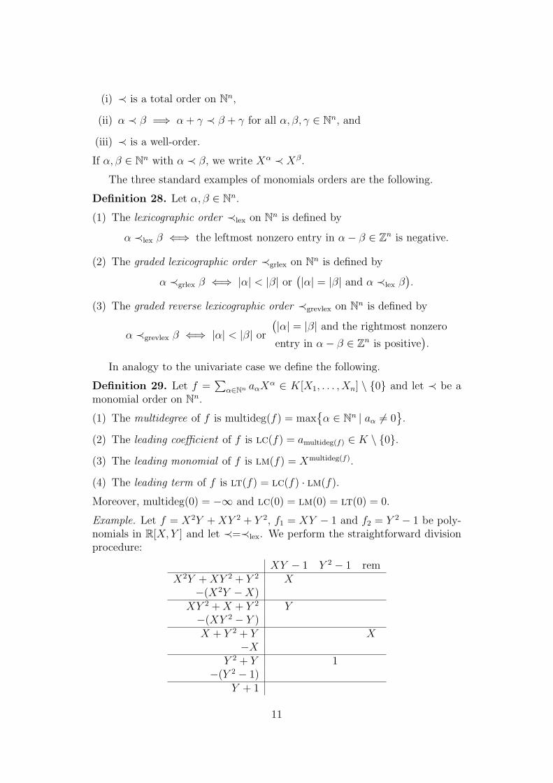
Example. Let f = X2Y + XY 2 + Y 2, f1 = XY − 1 and f2 = Y 2 − 1 be poly-nomials in R[X, Y ] and let ≺=≺lex. We perform the straightforward divisionprocedure:

XY − 1 Y 2 − 1 remX2Y + XY 2 + Y 2 X

−(X2Y −X)XY 2 + X + Y 2 Y−(XY 2 − Y )X + Y 2 + Y X

−XY 2 + Y 1

−(Y 2 − 1)Y + 1

11

Note that in the second step we could have used f2 for division as well. In thethird step a phenomenon occured that cannot happen in the univariate case.The leading term X is not divisible by any of lt(f1) and lt(f2), whereas thereare still terms in X + Y 2 + Y that are divisible by them. Therefore we movedX to the remainder column. From the above table we conclude

f = (X + Y ) · f1 + 1 · f2 + (X + Y + 1).

Algorithm 30 (Division Algorithm).Input: f, f1, . . . , fs ∈ K[X1, . . . , Xn] \ {0} and a monomial order ≺.Output: q1, . . . , qs, r ∈ K[X1, . . . , Xn] such that f = q1f1 + · · ·+ qsfs + r andno term in r is divisible by any of lt(f1), . . . , lt(fs). Moreover, multideg(f) <multideg(qifi) for all i = 1, . . . , s.

(1) p← f, r ← 0, for i = 1, . . . , s do qi ← 0

(2) while p 6= 0 do

• if lt(fi) | lt(p) for a minimal i ∈ {1, . . . , s} then

qi ← qi +lt(p)

lt(fi), p← p− lt(p)

lt(fi)· fi

• elser ← r + lt(p), p← p− lt(p)

(3) return q1, . . . , qs, r

Proof of correctness. At each entry to the while-loop the following invariantshold:

(i) f = p + q1f1 + · · ·+ qsfs + r,

(ii) no term in r is divisible by any of lt(f1), . . . , lt(fs), and

(iii) multideg(f) < multideg(qifi) for all i = 1, . . . , s.

The algorithm terminates if eventually p = 0. If p is redefined to be p′ 6= 0during the while-loop, then

multideg(p′) ≺ multideg(p).

Therefore p = 0 must finally happen, because otherwise we would get an infi-nite decreasing sequence of multidegrees contradicting the well-order propertyof ≺.

The remainder on division of f by the s-tuple F = (f1, . . . , fs) is denotedby

fF.

The Division Algorithm has a major drawback: the remainder fF

need not beunique and depends on the order of f1, . . . , fs. In particular it may happen

that f ∈ 〈f1, . . . , fs〉 and still fF 6= 0. Grobner bases are special generating

sets that overcome these problems.

12

3.2 Existence and Uniqueness

Definition 31. An ideal I E K[X1, . . . , Xn] is called monomial ideal if thereis a subset A ⊆ Nn such that

I = 〈XA〉 := 〈Xα | α ∈ A〉.

The key property of monomial ideals is the following lemma.

Lemma 32. Let A ⊆ Nn be a subset, I = 〈XA〉 E K[X1, . . . , Xn] a monomialideal and β ∈ Nn. Then

Xβ ∈ I ⇐⇒ ∃α ∈ A : Xα | Xβ.

Proof. Let Xβ ∈ I. Then there are q1, . . . , qs ∈ K[X1, . . . , Xn] and α1, . . . , αs ∈A such that Xβ =

∑si=1 qiX

αi . Therefore Xβ occurs in at least one of the qiXαi

and hence Xαi | Xβ.The converse implication is obvious.

Lemma 33 (Dickson). Let A ⊆ Nn be a subset and I = 〈XA〉 E K[X1, . . . , Xn]a monomial ideal. Then there exists a finite subset B ⊆ A such that

〈XA〉 = 〈XB〉.

Proof. This follows immediately from Corollary 11.

Dickson’s Lemma motivates the following definition.

Definition 34. Let I E K[X1, . . . , Xn] be an ideal and let ≺ be a monomialorder on Nn. A finite set G ⊆ I is a Grobner basis for I with respect to ≺ if

〈lt(G)〉 = 〈lt(I)〉.

Theorem 35. Let ≺ be a monomial order on Nn. Then every ideal I EK[X1, . . . , Xn] has a Grobner basis G w.r.t. ≺. Moreover,

I = 〈G〉.

Proof. The first statement follows directly from Dickson’s Lemma. For thesecond statement let f ∈ I and G = {g1, . . . , gt}. The Division Algorithmyields q1, . . . , qt, r ∈ K[X1, . . . , Xn] such that f = q1g1 + · · ·+ qtgt + r and noterm of r is divisible by any of lt(g1), . . . , lt(gt). But r = f−q1g1−· · ·−qtgt ∈I and hence lt(r) ∈ lt(I) = 〈lt(G)〉. From Lemma 32 it follows that r = 0and thus f ∈ 〈G〉.

For Grobner bases, the Division Algorithm yields a unique remainder.

Theorem 36. Let I E K[X1, . . . , Xn] be an ideal and let G be a Grobner basisfor I. Let f ∈ K[X1, . . . , Xn]. Then there is a unique r ∈ K[X1, . . . , Xn] suchthat

13

(i) f − r ∈ I, and

(ii) no term of r is divisble by any term in lt(G).

In particular, r = fG

is the remainder on division of f by G and is called thenormal form of f with respect to G.

Proof. The Division Algorithm proves the existence of an r with the desiredproperties. For the uniqueness, let g, g′ ∈ I and r, r′ ∈ K[X1, . . . , Xn] suchthat f = g + r = g′ + r′ and both r and r′ satisfy (ii). Then r− r′ = g′− g ∈ Iand hence lt(r − r′) ∈ 〈lt(I)〉 = 〈lt(G)〉. By Lemma 32, there is a g ∈ Gwith lt(g) | lt(r − r′). Therefore r − r′ = 0.

In general, an ideal can have many different Grobner bases. By the fol-lowing observation, there may be elements in a Grobner basis that can beeliminated.

Lemma 37. Let I E K[X1, . . . , Xn] be an ideal and let G be a Grobner basisfor I. If g ∈ G such that

lt(g) ∈⟨lt(G \ {g})

⟩,

then G \ {g} is also a Grobner basis for I.

Definition 38. Let I E K[X1, . . . , Xn] be an ideal. A Grobner basis G for Iis called minimal if for all g ∈ G

(i) lc(g) = 1, and

(ii) lt(g) 6∈⟨lt(G \ {g})

⟩.

An ideal might still have many different minimal Grobner bases G. If wereplace each g ∈ G by the reduced element gG\{g}, we obtain a unique basis.

Definition 39. Let I E K[X1, . . . , Xn] be an ideal and let G be a Grobnerbasis for I. An element g ∈ G is called reduced with respect to G if no term ofg is in ⟨

lt(G \ {g})⟩.

G is called reduced if G is minimal and every g ∈ G is reduced with respect toG.

Theorem 40. Every ideal I E K[X1, . . . , Xn] has a unique reduced Grobnerbasis.

14

3.3 Buchberger’s Algorithm

The proof of the existence of Grobner bases was non-constructive. We are noteven able to detect wether a given generating set G = {g1, . . . , gt} is a Grobnerbasis. One reason why G might fail to be a Grobner basis could be a linearcombination of the gi whose leading term is not in 〈lt(G)〉 due to cancellationof leading terms of the gi. The S-polynomial of two polynomials f and g isdefined in such a way that the leading terms of f and g cancel.

Definition 41. Let f, g ∈ K[X1, . . . , Xn]\{0} and let Xγ = lcm(lm(f), lm(g)

).

Then the S-polynomial of f and g is

S(f, g) =Xγ

lt(f)· f − Xγ

lt(g)· g.

The following theorem shows that every kind of cancellation can be ac-counted for by S-polynomials.

Theorem 42 (Buchberger 1965). A finite set G = {g1, . . . , gt} ⊆ K[X1, . . . , Xn]is a Grobner basis for the ideal 〈G〉 if and only if

S(gi, gj)G

= 0 (∗)

for all 1 ≤ i < j ≤ t.

Proof. If G is a Grobner basis then (∗) is fulfilled because of the uniquenessproperty in Theorem 36.

Conversely, suppose that (∗) holds. Assume by way of contradiction thatG is not a Grobner basis. Then there is an f ∈ I with lt(f) /∈ 〈lt(G)〉. Wechoose q1, . . . , qt ∈ K[X1, . . . , Xn] such that

f = q1g1 + · · ·+ qtgt

and both

(i) δ := max{multideg(q1g1), . . . , multideg(qtgt)

}, and

(ii) k :=∣∣{qigi | multideg(qigi) = δ and 1 ≤ i ≤ t

}∣∣are minimal. This is possible because≺ is a well-order. We may assume w.l.o.g.that multideg(q1g1) = . . . = multideg(qkgk) = δ and multideg(qigi) ≺ δ fork < i ≤ t. Since lt(f) is not divisible by any term in lt(G), the termsin the qigi that contain the monomial Xδ must cancel, in particular k ≥ 2.For i = 1, 2 we denote lt(qigi) = aibi, where ai and bi are terms in qi andgi respectively. Since a1b1 = c · a2b2 for some c ∈ K, there is a polynomialr ∈ K[X1, . . . , Xn] such that

r · lcm(b1, b2)

b1

= a1.

15

By (∗), there are r1, . . . , rt ∈ K[X1, . . . , Xn] such that

S(g1, g2) = r1g1 + · · ·+ rtgt

and multideg(S(g1, g2)

)< multideg(rigi) for i = 1, . . . , t. Expanding the

expression

f = f − r(S(g1, g2)−

∑ti=1 rigi

)= q′1g1 + · · ·+ q′tgt

for some q′1, . . . , q′t ∈ K[X1, . . . , Xn] yields a representation of f such that

multideg(q′2g2) = . . . = multideg(q′kgk) = δ and multideg(qigi) ≺ δ for i = 1and k < i ≤ t. This contradicts the minimality of k.

Buchberger’s criterion naturally leads to the following algorithm.

Algorithm 43 (Buchberger’s Algorithm).Input: f1, . . . , fs ∈ K[X1, . . . , Xn] and a monomial order ≺.Output: A Grobner basis G for the ideal I = 〈f1, . . . , fs〉 w. r. t. ≺ such thatf1, . . . , fs ∈ G.

(1) G← {f1, . . . , fs}

(2) repeat

(a) S ← ∅(b) for each {g, g′} ⊆ G with g 6= g′ do

• r ← S(g, g′)G

• if r 6= 0 then S ← S ∪ {r}(c) G← G ∪ S

until S = ∅

(3) return G

Proof of correctness. At each stage of the algorithm G ⊆ I holds, and sincef1, . . . , fs ∈ G, we also have 〈G〉 = I. The algorithm terminates if eventually

S(g, g′)G

= 0

for all g, g′ ∈ G with g 6= g′. Then G is a Grobner basis for I by Theorem 42.Assume that G is redefined to be G′ with G ( G′ during the repeat-until-

loop. Then there is an r ∈ G′ such that no term in r is divisible by any termin lt(G). Hence lt(r) /∈ 〈lt(G)〉 but lt(r) ∈ 〈lt(G′)〉, and therefore

〈lt(G)〉 ( 〈lt(G′)〉.

Thus the algorithm must finally terminate, because otherwise we get an infi-nite proper ascending chain of ideals in contradiction to K[X1, . . . , Xn] beingNoetherian.

16

3.4 Applications

The uniqueness of the remainder on division by a Grobner basis and the unique-ness of reduced Grobner bases solves the ideal membership and the consistencyproblem respectively.

Proposition 44. Let I E K[X1, . . . , Xn] be an ideal and let G be a Grobnerbasis for I. Let f ∈ K[X1, . . . , Xn], then

f ∈ I ⇐⇒ fG

= 0.

Proposition 45. Let I E K[X1, . . . , Xn] be an ideal and let G be the reducedGrobner basis for I. Then

1 ∈ I ⇐⇒ G ={1}.

By applying the Rabinovich trick, we can reduce the radical membershipproblem to the consistency problem.

Proposition 46. Let I = 〈f1, . . . , fs〉 E K[X1, . . . , Xn] be an ideal and letf ∈ K[X1, . . . , Xn]. Define

J := 〈f1, . . . , fs, Xn+1f − 1〉 E K[X1, . . . , Xn+1].

Thenf ∈√

I ⇐⇒ 1 ∈ J.

Proof. If 1 ∈ J then we obtain f ∈√

I like in the proof of the Strong Null-stellensatz.

Conversely, let f ∈√

I. Then there is an e ∈ N>0 such that f e ∈ I ⊆ J .Therefore

1 = Xen+1f

e − (Xen+1f

e − 1)

= Xen+1f

e − (Xe−1n+1f

e−1 + · · ·+ Xn+1f + 1)(Xn+1f − 1) ∈ J.

Grobner bases are also useful for solving systems of polynomial equationsbecause of elimination properties of the ≺lex order.

Definition 47. Let I E K[X1, . . . , Xn] be an ideal. The `-th elimination idealI` is defined by

I` = I ∩K[X`+1, . . . , Xn].

Theorem 48 (Elimination Theorem). Let I E K[X1, . . . , Xn] be an ideal andlet G be a Grobner basis for I with respect to ≺lex. Then

G` = G ∩K[X`+1, . . . , Xn]

is a Grobner basis for I`.

17

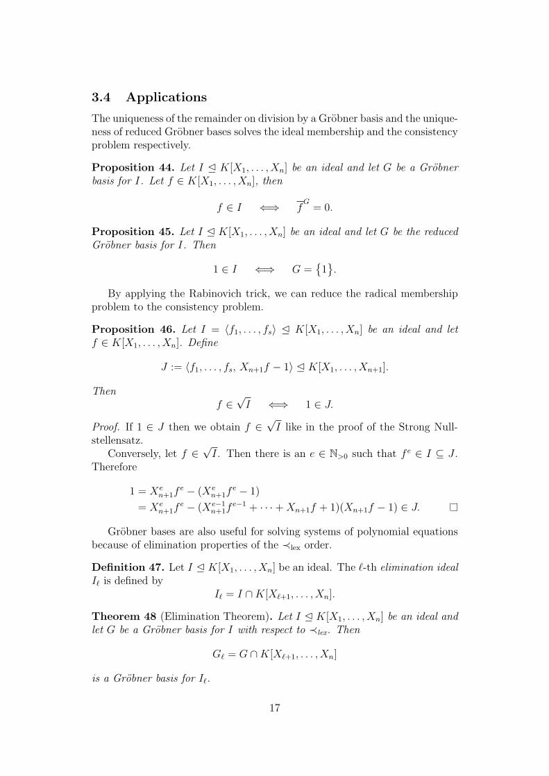
Example. Recall the graph G = (V, E) from the introductory example:

1

2

3

4

Let

I =⟨X3

i − 1 | i ∈ V⟩

+⟨X2

i + XiXj + X2j | (i, j) ∈ E

⟩E C[X1, . . . , X4].

The reduced Grobner basis for I w. r. t. ≺lex is G = {g1, . . . , g4} with

g1 = X1 −X4,

g2 = X2 + X3 + X4,

g3 = X23 + X3X4 + X2

4 ,

g4 = X34 − 1.

From the triangular form we find that for instance(1, e(2/3)πi, e(4/3)πi, 1

)∈

Var(I).

The following proposition together with the Elimination Theorem showshow to compute the intersection of ideals.

Proposition 49. Let I, J E K[X1, . . . , Xn] be ideals. Then

I ∩ J =(X0 · I + (1−X0) · J

)∩K[X1, . . . , Xn].

Proof. Let f ∈ I ∩ J . Then

f = X0f + (1−X0)f ∈(X0 · I + (1−X0) · J

)∩K[X1, . . . , Xn].

Conversely, let f ∈(X0 · I + (1−X0) · J

)∩K[X1, . . . , Xn]. Then there are

f1 ∈ I and f2 ∈ J such that f = X0f1 + (1−X0)f2 ∈ K[X1, . . . , Xn]. SettingX0 = 1 and X0 = 0 yields f = f1 ∈ I and f = f2 ∈ J respectively, hencef ∈ I ∩ J .

4 Computational Complexity

In this section we want to discuss the computational complexity of the threedecision problems we encountered so far. A survey on complexity results aboutpolynomial ideals is given in [Ma97].

Definition 50. We define the following decision problems using a suitablecoding in sparse representation:

18

(1) The ideal membership problem is defined by

IM ={(f, f1, . . . , fs) ∈ (Q[X1, . . . , Xn])s+1 | f ∈ 〈f1, . . . , fs〉

}.

(2) The consistency problem is defined by

Cons ={(f1, . . . , fs) ∈ (Q[X1, . . . , Xn])s | 1 ∈ 〈f1, . . . , fs〉

}.

(3) The radical membership problem is defined by

RM ={(f, f1, . . . , fs) ∈ (Q[X1, . . . , Xn])s+1 | f ∈

√〈f1, . . . , fs〉

}.

Lower bounds of the complexity of those problems yield lower bounds forthe complexity of Buchberger’s Algorithm. Recall the standard complexityclasses

P ⊆ NP ⊆ PSPACE ⊆ EXP ⊆ NEXP ⊆ EXPSPACE

(for a definition, see e. g. [Pa94]).

4.1 Degree Bounds

An upper bound for IM can be obtained by the following degree bound whichis double exponential in the number of variables.

Theorem 51 (Hermann 1926). Let I = 〈f1, . . . , fs〉 E Q[X1, . . . , Xn] be anideal and let d = max

{deg(f1), . . . , deg(fs)

}.

If f ∈ I then there are q1, . . . , qs ∈ Q[X1, . . . , Xn] such that f = q1f1 +· · ·+ qsfs and

deg(qi) ≤ deg(f) + (sd)2n

for all i = 1, . . . , s.

Using this bound it is possible to enumerate all monomials that can appearin the qi, what leads to a system of linear equations. Therefore IM can bereduced to a rank computation of a matrix of size double exponential in theinput size. For the latter problem there exist algorithms on a parallel ran-dom access machine (PRAM) with a polynomial number of processors usingpolylogarithmic time. By the Parallel Computation Thesis (parallel time =sequential space) this yields an algorithm in exponential space. However, thematrix is too large and cannot be written down in exponential space. But in[Ma89] it is shown that the entries of the matrix can be generated on the flyfrom the polynomial description and that this does not affect the algorithmfor the rank computation.

Theorem 52 (Mayr 1989).

IM ∈ EXPSPACE.

19

For Cons the upper degree bound can be improved to be single exponentialin the number of variables. Again, by the Rabinovich trick, this also yields anupper bound for RM.

Theorem 53 (Brownawell 1987). Let I = 〈f1, . . . , fs〉 E Q[X1, . . . , Xn] be anideal, µ = min{s, n} and d = max

{deg(f1), . . . , deg(fs)

}.

(1) If the fi have no common zero in Cn, then there are q1, . . . , qs ∈ Q[X1, . . . , Xn]with 1 = q1f1 + · · ·+ qsfs such that

deg(qi) ≤ µndµ + µd for i = 1, . . . , s.

(2) If f ∈ Q[X1, . . . , Xn] such that f(ξ) = 0 for all common zeros ξ of thefi in Cn, then there are e ∈ N>0 and q1, . . . , qs ∈ Q[X1, . . . , Xn] withf e = q1f1 + · · ·+ qsfs such that

e ≤ (µ + 1)(n + 2)(d + 1)µ+1 and

deg(qi) ≤ (µ + 1)(n + 2)(d + 1)µ+2 for i = 1, . . . , s.

With similar techniques, these bounds can be used to show the followingresult.

Corollary 54.

Cons ∈ PSPACE and RM ∈ PSPACE.

Finally, we want to mention a degree bound for the polynomials in thereduced Grobner basis of an ideal.

Theorem 55 (Dube 1990). Let I = 〈f1, . . . , fs〉 E K[X1, . . . , Xn] be an idealand let d = max

{deg(f1), . . . , deg(fs)

}.

Then for any monomial order, the total degree of polynomials in the reducedGrobner basis for I is bounded above by

2(d2

2+ d

)2n−1

.

4.2 Mayr–Meyer Ideals

In [MM82], Mayr and Meyer showed that Hermann’s double exponential degreebound is asymptotically tight. We show a slightly modified construction from[BS88]. Let n ∈ N. For r ∈ N we define er := 22r

. Then

er = (er−1)2 for all r ∈ N>0.

We construct an ideal in the polynomial ring R over Q with the 10n variables

Sr start

Fr finish

Br,1, . . . , Br,4 counters

Cr,1, . . . , Cr,4 catalysts

20

for each level r = 0, . . . , n. For notational convenience, we will omit subscriptsfrom now on if r is fixed. Upper-case letters denote variables of level r andlower-case letters denote variables of level r − 1. For r = 0 we define I0 E Rto be generated by

SCi − FCiB2i for i = 1, . . . , 4.

If r > 0, then Ir E R is generated by Ir−1 and

S − sc1, sc4 − F,

fc1 − sc2, sc3 − fc4,

fc2b1 − fc3b4, sc3 − sc2,

fc2Cib2 − fc2CiBib3 for i = 1, . . . , 4.

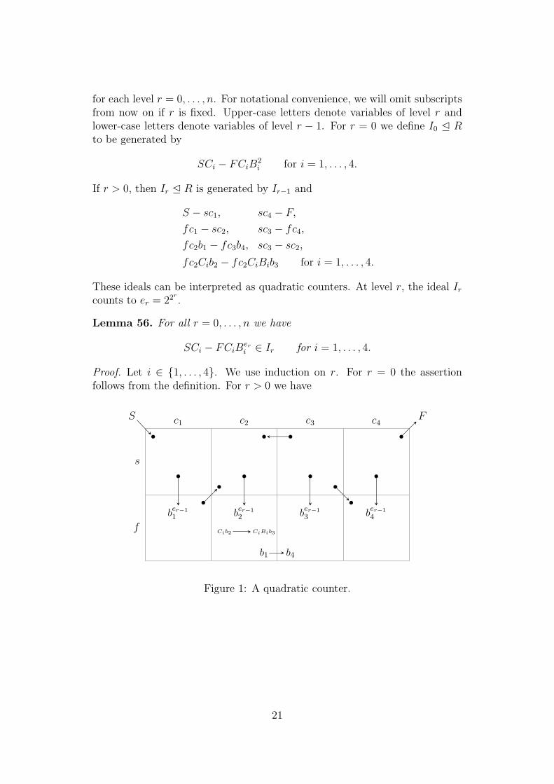
These ideals can be interpreted as quadratic counters. At level r, the ideal Ir

counts to er = 22r.

Lemma 56. For all r = 0, . . . , n we have

SCi − FCiBeri ∈ Ir for i = 1, . . . , 4.

Proof. Let i ∈ {1, . . . , 4}. We use induction on r. For r = 0 the assertionfollows from the definition. For r > 0 we have

s

f

c1 c2 c3 c4S

ber−1

1 ber−1

2

Cib2 CiBib3

b1 b4

ber−1

3 ber−1

4

F

Figure 1: A quadratic counter.

21

SCi = sc1Ci

= fc1Ciber−1

1 by induction

= sc2Ciber−1

1

= fc2Ciber−1

1 ber−1

2 by induction

= . . .

= fc2CiBer−1

i ber−1

1 ber−1

3

= fc3CiBer−1

i ber−1−11 b

er−1

3 b4

= sc3CiBer−1

i ber−1−11 b4 by induction

= sc2CiBer−1

i ber−1−11 b4

= fc2CiB2er−1

i ber−1−11 b

er−1

2 b4 by induction

= . . .

= fc2CiB2er−1

i ber−1−11 b

er−1

3 b4

= fc3CiB2er−1

i ber−1−21 b

er−1

3 b24

= sc3CiB2er−1

i ber−1−21 b2

4 by induction

= . . . repeating the previous 7 lines

er−1 − 2 times

= sc3CiBe2r−1

i ber−1

4

= fc4CiBe2r−1

i ber−1

4

= fc4CiBe2r−1

i by induction

= FCiBeri (mod Ir).

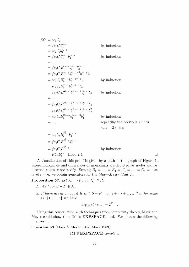
A visualization of this proof is given by a path in the graph of Figure 1,where monomials and differences of monomials are depicted by nodes and bydirected edges, respectively. Setting B1 = . . . = B4 = C1 = . . . = C4 = 1 atlevel r = n, we obtain generators for the Mayr–Meyer ideal Jn.

Proposition 57. Let Jn = 〈f1, . . . , fs〉 E R.

1. We have S − F ∈ Jn.

2. If there are q1, . . . , qs ∈ R with S − F = q1f1 + · · ·+ qsfs, then for somei ∈ {1, . . . , s} we have

deg(qi) ≥ en−1 = 22n−1

.

Using this construction with techniques from complexity theory, Mayr andMeyer could show that IM is EXPSPACE-hard. We obtain the followingfinal result.

Theorem 58 (Mayr & Meyer 1982, Mayr 1989).

IM ∈ EXPSPACE-complete.

22

References

[BS88] D. Bayer and M. Stillman. On the complexity of computing syzygies.J. Symb. Comput. 6, 135–147, 1988.

[Bro87] W.D. Brownawell. Bounds for the degrees in the Nullstellensatz.Ann. of Math. 126, 577–591, 1987.

[Bu65] B. Buchberger. Ein Algorithmus zum Auffinden der Basiselementedes Restklassenringes nach einem nulldimensionalen Polynomideal.PhD thesis, Leopold-Franzens-Universitat Innsbruck, Austria, 1965.

[CLO97] D. Cox, J. Little and D. O’Shea. Ideals, Varieties, and Algorithms.Springer-Verlag, New York, 2nd edition, 1997.

[Du90] T.W. Dube. The structure of polynomial ideals and Grobner bases.SIAM J. Comput. 19 (4), 750–775, 1990.

[Eis95] D. Eisenbud. Commutative Algebra with a View Toward AlgebraicGeometry. Springer-Verlag, New York, 1995.

[vzGG03] J. von zur Gathen and J. Gerhard. Modern Computer Algebra. Uni-versity Press, Cambridge, 2nd edition, 2003.

[He26] G. Hermann. Die Frage der endlich vielen Schritte in der Theorieder Polynomideale. Math. Ann. 95, 736–788, 1926.English translation: The question of finitely many steps in polyno-mial ideal theory. SIGSAM Bull. 32 (3), 8–30, 1998.

[La05] S. Lang. Algebra. Springer-Verlag, New York, 3rd edition, 2005.

[Ma89] E.W. Mayr. Membership in Polynomial Ideals over Q Is ExponentialSpace Complete. Proc. of the 6th Ann. Symp. on Theoretical Aspectsof Computer Science STACS ’89, Paderborn, eds. B. Monien andR. Cori, LNCS 349, Springer Verlag, 400–406, 1989.

[Ma97] E.W. Mayr. Some complexity results for polynomial ideals. J. ofComplexity 13 (3), 303–325, 1997.

[MM82] E.W. Mayr and A.R. Meyer. The Complexity of the Word Problemsfor Commutative Semigroups and Polynomial Ideals. Advances inMath. 46, 305–329, 1982.

[Pa94] C.H. Papadimitriou. Computational Complexity. Addison-Wesley,1994.

23