Gravity:

• Gravity anomalies.

• Earth gravitational field.

• Isostasy.

• Moment density dipole.

• Practical issues.

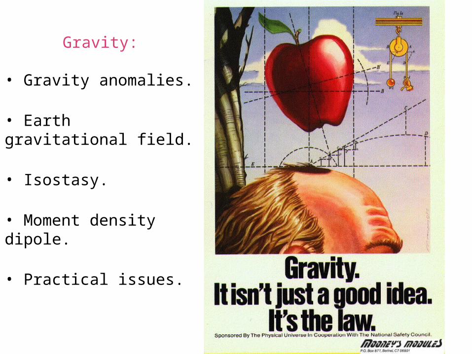
Newton’s law of gravitation:

where:• F is the force of gravitation.• m1 and m2 are the masses.• r is the distance between the masses.• is the gravitational constant that is equal to 6.67x10-11 Nm2kg-2 (fortunately is a small number).

Units of F are N=kg m s-2 .

The basics

€

F = γm1m2

r2 ,

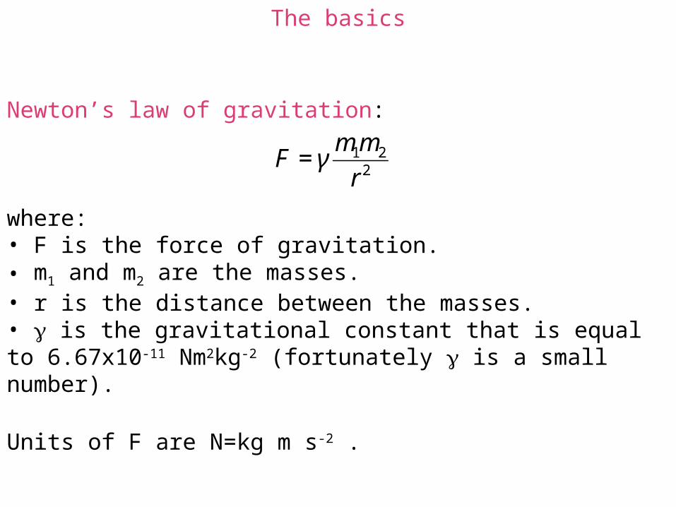
Newton’s second law of motion:

where:• m is the mass.• a is acceleration.

By combining the universal law of gravitation with Newton’s second law of motion, one finds that the acceleration of m2 due to its attraction by m1 is:

The basics

€

F = ma ,

€

a =γm1

r2 .

Gravitational acceleration is thus:

where:• ME is the mass of the Earth.• RE is the Earth’s radius.

Units of acceleration are m s-2, or gal=0.01 m s-2.

The basics

€

g =γME

RE2 ,

Question: Is earth gravitational field greater at the poles or at the equator?

Question: Is earth gravitational field a constant?

The basics

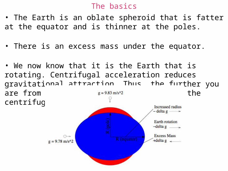
• The Earth is an oblate spheroid that is fatter at the equator and is thinner at the poles.

• There is an excess mass under the equator.

• We now know that it is the Earth that is rotating. Centrifugal acceleration reduces gravitational attraction. Thus, the further you are from the rotation axis, the greater the centrifugal acceleration is.

The basics

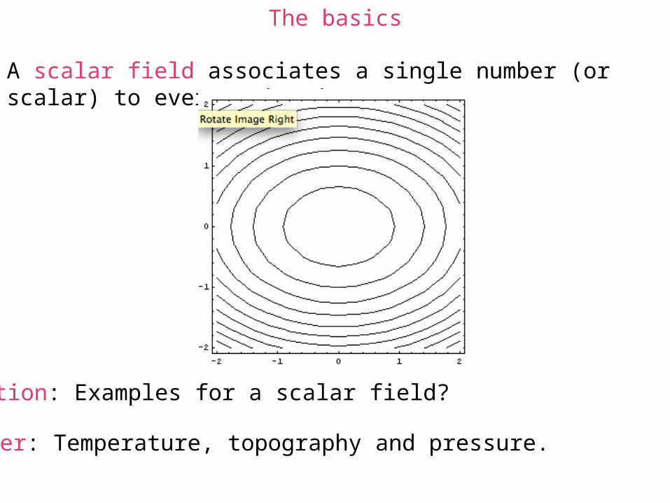
A scalar field associates a single number (or scalar) to every point in space.

Question: Examples for a scalar field?

Answer: Temperature, topography and pressure.

The basics

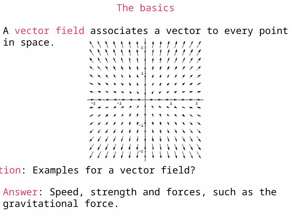
A vector field associates a vector to every point in space.

Question: Examples for a vector field?

Answer: Speed, strength and forces, such as the gravitational force.

The basics

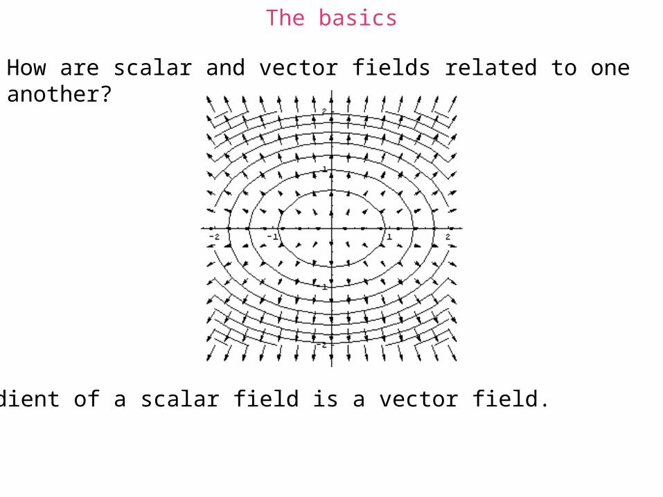
How are scalar and vector fields related to one another?

The gradient of a scalar field is a vector field.

The basics

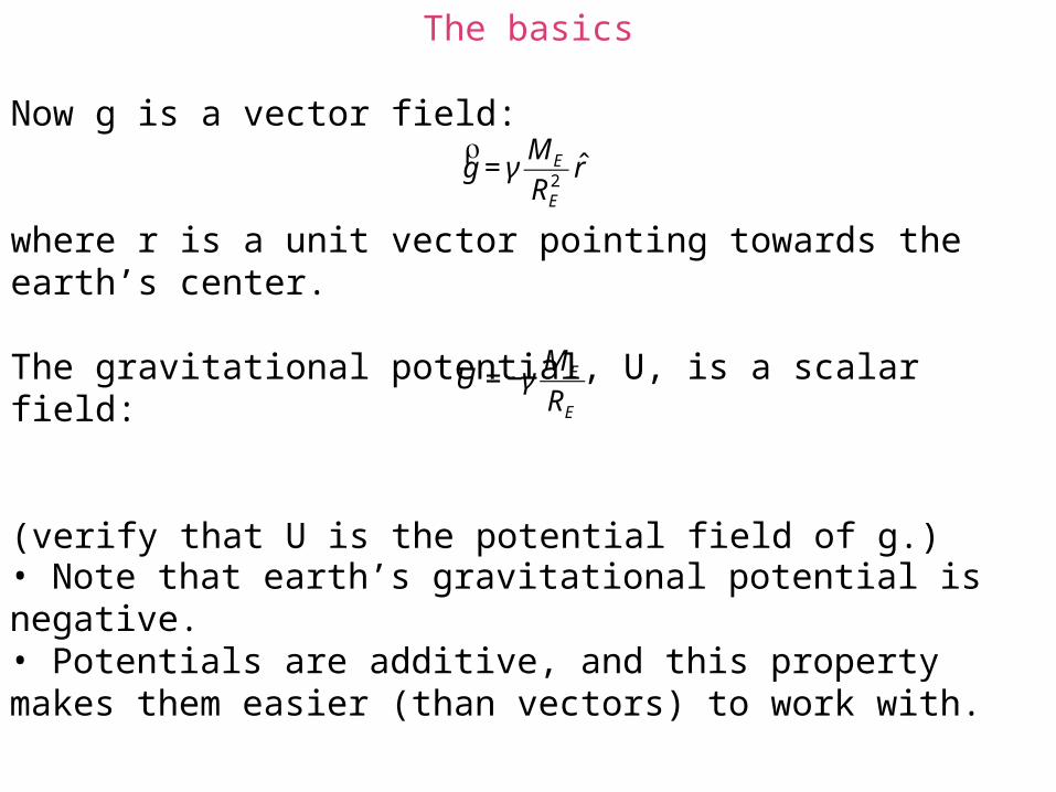
Now g is a vector field:

where r is a unit vector pointing towards the earth’s center.

The gravitational potential, U, is a scalar field:

(verify that U is the potential field of g.)

• Note that earth’s gravitational potential is negative.• Potentials are additive, and this property makes them easier (than vectors) to work with.

€

rg = γ

ME

RE2

ˆ r ,

€

U = −γME

RE

.

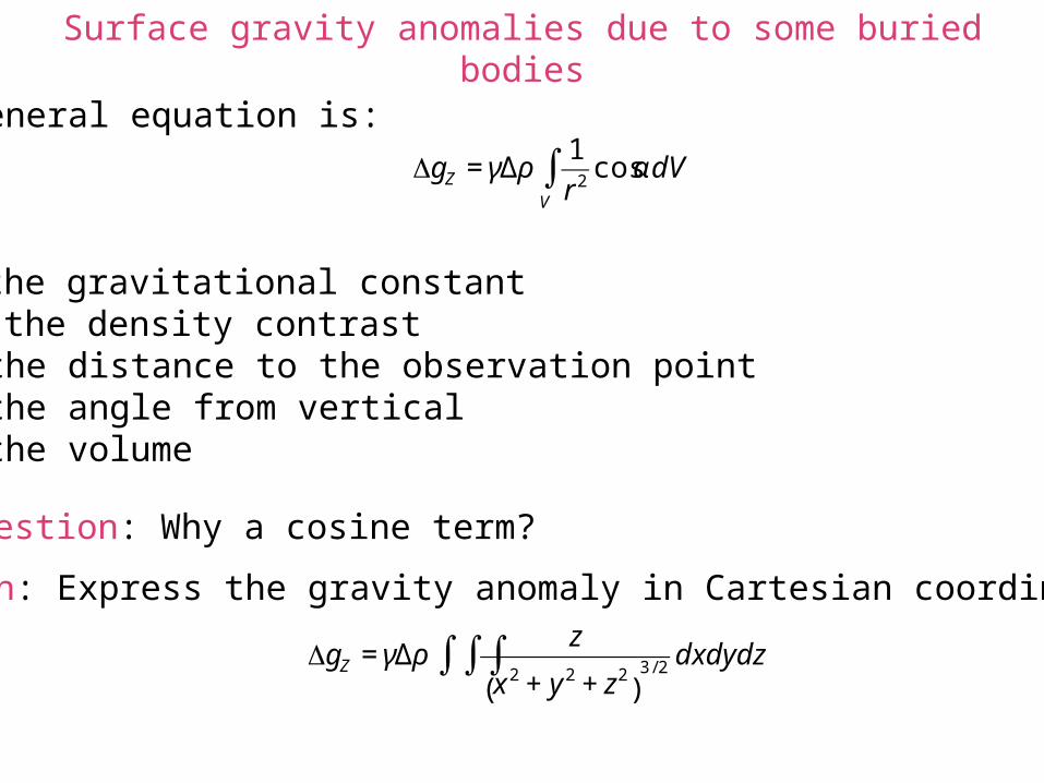
Surface gravity anomalies due to some buried bodies

The general equation is:

where: is the gravitational constant is the density contrastr is the distance to the observation pointa is the angle from verticalV is the volume

Question: Express the gravity anomaly in Cartesian coordinates.

€

gZ = γΔρ1

r2cosαdV ,

V

∫

Question: Why a cosine term?

€

gZ = γΔρz

x 2 + y 2 + z2( )

3 / 2 dxdydz∫∫∫ .

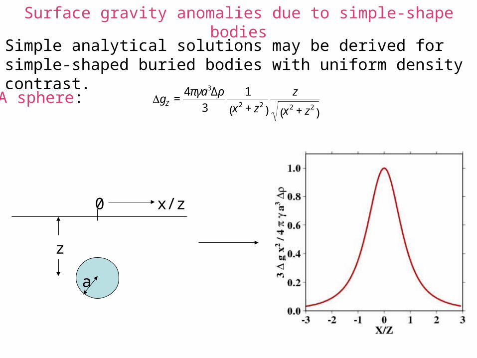
Surface gravity anomalies due to simple-shape bodies

€

gZ =4πγa3Δρ

3

1

x 2 + z2( )

z

x 2 + z2( )

.A sphere:

z

a

0 x/z

Simple analytical solutions may be derived for simple-shaped buried bodies with uniform density contrast.

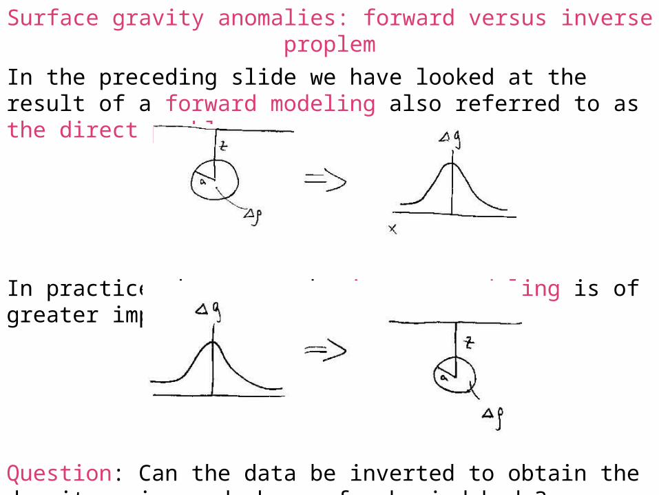
Surface gravity anomalies: forward versus inverse proplem

In the preceding slide we have looked at the result of a forward modeling also referred to as the direct problem:

In practice, however, the inverse modeling is of greater importance:

Question: Can the data be inverted to obtain the density, size and shape of a buried body?

Surface gravity anomalies: forward versus inverse problem

• Inspection of the solution for a buried sphere reveals a non-uniqueness of that problem. The term a3 introduces an ambiguity to the problem. This is because there are infinite combinations of and a3 that give the same a3.

• This highlights the importance of adding geological and geophysical constraints!

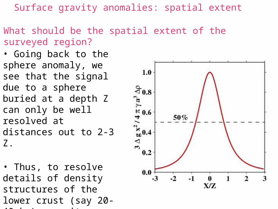
Surface gravity anomalies: spatial extent

What should be the spatial extent of the surveyed region?

• Going back to the sphere anomaly, we see that the signal due to a sphere buried at a depth Z can only be well resolved at distances out to 2-3 Z.

• Thus, to resolve details of density structures of the lower crust (say 20-40 km), gravity measurements must be made over an extensive area.

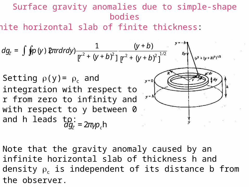
Surface gravity anomalies due to simple-shape bodies

An infinite horizontal slab of finite thickness:

€

dgZ = γρ (y)(2πrdrdy )1

r2 + (y + b)2[ ]

(y + b)

r2 + (y + b)2[ ]

1/ 2∫∫ .

Setting (y)= c and integration with respect to r from zero to infinity and with respect to y between 0 and h leads to:

€

dgZ = 2πγρ ch .

Note that the gravity anomaly caused by an infinite horizontal slab of thickness h and density c is independent of its distance b from the observer.

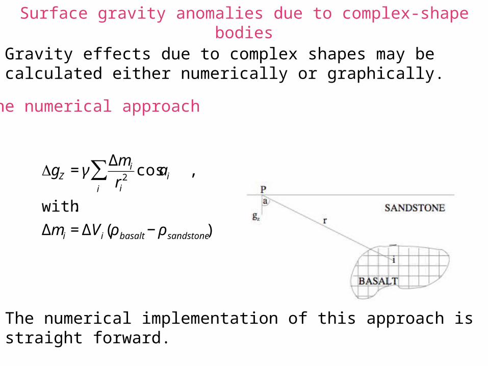
Surface gravity anomalies due to complex-shape bodies

€

gZ = γΔmi

ri2

cosai

i

∑ ,

with :

Δmi = ΔVi(ρ basalt − ρ sandstone) .

The numerical approach

Gravity effects due to complex shapes may be calculated either numerically or graphically.

The numerical implementation of this approach is straight forward.

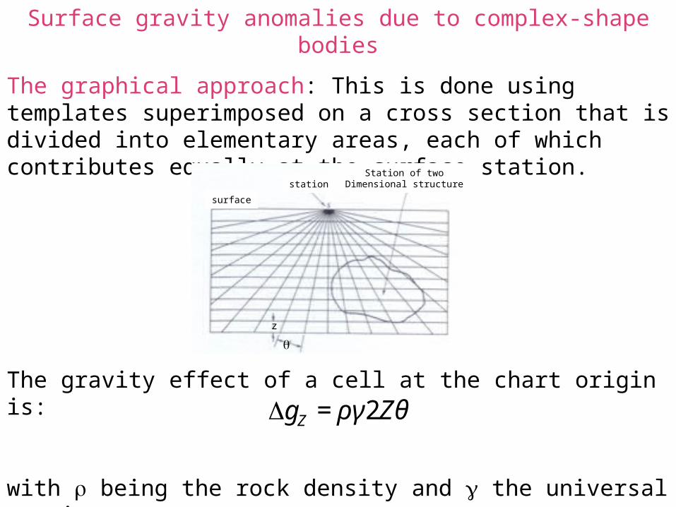
Surface gravity anomalies due to complex-shape bodies

The graphical approach: This is done using templates superimposed on a cross section that is divided into elementary areas, each of which contributes equally at the surface station.

The gravity effect of a cell at the chart origin is:

with being the rock density and the universal gravity constant.

€

gZ = ργ2Zθ ,

surface

stationStation of two

Dimensional structure

z