GRASS GIS for Geomorphologists:

An Introductory Guide

Andrew Wickert

April 16, 2012

2

Contents

1 Introduction 71.1 GIS . . . . . . . . . . . . . . . . . . . . . . . . . . . . . . . . . . 71.2 What is GRASS? . . . . . . . . . . . . . . . . . . . . . . . . . . . 8

1.2.1 GRASS Interfaces . . . . . . . . . . . . . . . . . . . . . . 81.2.2 Topology . . . . . . . . . . . . . . . . . . . . . . . . . . . 91.2.3 File structure . . . . . . . . . . . . . . . . . . . . . . . . . 9

2 Downloading and Installing GRASS 112.1 Ubuntu (should work for Debian too) . . . . . . . . . . . . . . . 112.2 Mac OS X . . . . . . . . . . . . . . . . . . . . . . . . . . . . . . . 112.3 Windows 7 . . . . . . . . . . . . . . . . . . . . . . . . . . . . . . 13

2.3.1 Native Install . . . . . . . . . . . . . . . . . . . . . . . . . 132.3.2 Unix oriented . . . . . . . . . . . . . . . . . . . . . . . . . 13

3 Starting GRASS and Creating a Location 153.1 Starting GRASS . . . . . . . . . . . . . . . . . . . . . . . . . . . 153.2 Database manager . . . . . . . . . . . . . . . . . . . . . . . . . . 153.3 Creating a Location: Gordon Gulch . . . . . . . . . . . . . . . . 163.4 Starting a GRASS GIS session . . . . . . . . . . . . . . . . . . . 18

4 Basic Raster Display and Region Operations 234.1 Importing GDAL Raster Data . . . . . . . . . . . . . . . . . . . 234.2 Viewing and setting the region . . . . . . . . . . . . . . . . . . . 254.3 Displaying Raster Data . . . . . . . . . . . . . . . . . . . . . . . 26

4.3.1 Simple raster display with the command line . . . . . . . 264.3.2 Displaying raster (elevation and shaded relief) maps in

the graphical interface . . . . . . . . . . . . . . . . . . . . 264.3.3 Combining rasters for display in the command line: ele-

vation and shaded relief . . . . . . . . . . . . . . . . . . . 27

5 Topographic and hydrologic analyses 315.1 Slope, aspect, and resampling . . . . . . . . . . . . . . . . . . . 315.2 Drainage Networks . . . . . . . . . . . . . . . . . . . . . . . . . 325.3 Gordon Gulch drainage basin from set pour point . . . . . . . . 35

3

4 CONTENTS

5.4 Solar radiation . . . . . . . . . . . . . . . . . . . . . . . . . . . . 395.5 Cosmogenic dating . . . . . . . . . . . . . . . . . . . . . . . . . . 40

6 Vectors and databases 436.1 Vector topology . . . . . . . . . . . . . . . . . . . . . . . . . . . . 436.2 Managing databases and uploading vector attributes . . . . . . . 446.3 Advanced Vector and Database Processing . . . . . . . . . . . . . 45

6.3.1 Obtaining and cleaning points in stream networks . . . . 456.3.2 Queerying categories . . . . . . . . . . . . . . . . . . . . . 466.3.3 Extracting vector subsets . . . . . . . . . . . . . . . . . . 47

7 File input and output 517.1 Raster . . . . . . . . . . . . . . . . . . . . . . . . . . . . . . . . . 517.2 Vector . . . . . . . . . . . . . . . . . . . . . . . . . . . . . . . . . 527.3 Google Earth . . . . . . . . . . . . . . . . . . . . . . . . . . . . . 53

7.3.1 Coordinate transformation to lat/lon . . . . . . . . . . . . 537.3.2 Vector . . . . . . . . . . . . . . . . . . . . . . . . . . . . . 557.3.3 Raster . . . . . . . . . . . . . . . . . . . . . . . . . . . . . 557.3.4 Import into Google Earth . . . . . . . . . . . . . . . . . . 58

8 Writing and Executing Scripts 618.1 Text editors for programming . . . . . . . . . . . . . . . . . . . . 618.2 Shell scripting (Bash) . . . . . . . . . . . . . . . . . . . . . . . . 618.3 Python scripting . . . . . . . . . . . . . . . . . . . . . . . . . . . 63

9 Wrap-up 659.1 Thoughts from the Author . . . . . . . . . . . . . . . . . . . . . . 659.2 Useful Resources . . . . . . . . . . . . . . . . . . . . . . . . . . . 669.3 Future Plans . . . . . . . . . . . . . . . . . . . . . . . . . . . . . 669.4 Contact Information . . . . . . . . . . . . . . . . . . . . . . . . . 66

Boxes

1.1 Why GRASS? . . . . . . . . . . . . . . . . . . . . . . . . . . . . . 82.1 Good things to have for MacOS . . . . . . . . . . . . . . . . . . . 134.1 Help! . . . . . . . . . . . . . . . . . . . . . . . . . . . . . . . . . . 244.2 UNIX/GRASS terminal syntax . . . . . . . . . . . . . . . . . . . 254.3 Tips for the terminal . . . . . . . . . . . . . . . . . . . . . . . . . 305.1 GRASS GIS online (and o�ine) help . . . . . . . . . . . . . . . . 335.2 GRASS add-ons . . . . . . . . . . . . . . . . . . . . . . . . . . . 346.1 Specifying pour point locations by intersections . . . . . . . . . . 487.1 Image processing . . . . . . . . . . . . . . . . . . . . . . . . . . . 527.2 Latitude and Longitude in GRASS . . . . . . . . . . . . . . . . . 54

Notes

Original draft �nished 22 December 2011

First �nished draft completed on 16 April 2012

These notes are written for GRASS 6.4.X.

License

GRASS GIS for Geomorphologists: An Introductory Guide by Andrew D. Wick-ert is licensed under a Creative Commons Attribution-ShareAlike 3.0 UnportedLicense. You may freely use it, share it, and change it, so long as the authorgets some recognition. And if you want to change it, please let me know! I'dlove to have help in maintaining and/or expanding this manual.

5

6 BOXES

Chapter 1

Introduction

1.1 GIS

Most of you are probably familiar with GIS, and some of you probably useit very often. But for those of you who don't, GIS stands for "GeographicalInformation System". It is a software / programming language that is designedto work with data that are displayed spatially�in x,y,z or lat/lon,z coordinates.

Geospatial data take two main forms. Raster data are regularly-spacedCartesian grids. Vector data are speci�ed by sets of ungridded x,y,z pointsthat do not necessarily coincide with the position and spacing of raster grids.These can include points, lines, and areas. Raster and vector data types can beused in three dimensions as well, with three dimensional grids and the additionof volume-�lling vector elements. The most common geomorphic raster is thedigital elevation model (DEM); other common rasters are classi�ed land-usemaps and remotely sensed imagery: in general, they represent the intensity ofsome value across the whole region of interest. Common examples of vector datain geomorphology are river channels (lines), lakes (areas), and sample locations(points).

GIS packages contain a number of tools to work with raster and vectordata, make calculations based on them, perform �le input/output, reprojectdata from one coordinate system to another, manage databases of georeferencedinformation, and create human-readable maps to display the data that the GISpackage stores and processes.

Some reasons that geomorphologists use GIS are to:

1. Build maps

2. Display topographic data

3. Make calculations of topographic features (e.g., hypsometry, curvatures ofhillslopes)

4. Generate features involving water: lakes, rivers, drainage basins, shore-lines

7

8 CHAPTER 1. INTRODUCTION

5. Calculate regional values, such as insolation and 10Be production rates

6. Calculate and/or show regions of landscape change (e.g., erosion, deposi-tion, glacier retreat) over time

1.2 What is GRASS?

GRASS is the most popular open-source GIS package available. GRASS standsfor Geographic Resources Analysis Support System. It was �rst developed in1982 by the US Army Corps of engineers to be able to perform analyses forthe National Environmental Policy Act, with an emphasis on environmentalresearch and monitoring. It was released to the community in the early 90's,and has been a community-driven open source project ever since.

Why GRASS?I use GRASS because it is cross-platform (I am much more comfortableon UNIX-like systems than on Windows); it is very good at hydrologicanalyses; it is very scriptable for easy batch processing, sharing ofreproducible analyses, and geospatial integration of numerical models; itis open-source (so I can change components to �t my needs), and becauseI can share my work with anyone from around the world without beingtied down to expensive software.

On a personal note, I �nd programming in Windows to be a utterly hor-ri�c, time-wasting, and demoralizing experience. GRASS lets me stay ona UNIX-like OS, and this alone is reason enough for me to use it.

Box 1.1: Why GRASS?

Being open-source means that you can view and change all of the sourcecode�mostly C, with some bash and Python�in which it is written. WhileI have occasionally tweaked the source code for specialized projects, I almostnever have to: in my experience, GRASS is well-vetted and fully-functional.

For more information, go to http://grass.osgeo.org/.

1.2.1 GRASS Interfaces

GRASS is more of a computational / scripting GIS and less of a point-and-click GIS than ArcGIS. I �nd this to be an advantage, but for those of youwho like point-and-click there are a couple of options. GRASS now has a newinterface that is much improved from its old one, which is good for displayingdata. For editing vector �les, I have found Quantum GIS to be very nice: http://www.qgis.org/. It can work with GRASS data structures, and therefore beintegrated with your GRASS GIS project.

1.2. WHAT IS GRASS? 9

1.2.2 Topology

A major feature of GRASS is that it is a topological GIS. That is, it is impossibleto have small gaps or overlaps between vector areas (or �polygons�). It also forceslines to meet and interact according to some fairly logical rules. This helps forconsistency in geologic mapping and allows users to queery vector maps basedon their neighbors.

1.2.3 File structure

GRASS creates its own �le system. This is more rigid than the way that Archandles �les, but means that you will never lose your GIS �les, and you can takeyour whole folder with you as a bundle. File operations are handled internallyby GRASS. There are a large number of import/export options (GDAL, OGR,ASCII, etc.) that can be used to share your work with other GIS applications.I mention the �le system again in Section 3.3.

10 CHAPTER 1. INTRODUCTION

Chapter 2

Downloading and Installing

GRASS

Installation varies from a no-brainer to a di�cult task, depending on your op-erating system. I am going to be giving instructions for how to make the pre-compiled binaries work. Compiling your own version of GRASS is important ifyou want to change the source code and/or use the most updated version, but ittakes more work. (Pre-compiled binaries are the normal kinds of programs youwould install on a computer from a CD or the internet; compiling it yourselfmeans that you download the code and use a compiler, which turns this codeinto a binary program that your computer can run.) We will be downloadingand installing the stable release of GRASS, which right now is GRASS 6.4.1 orGRASS 6.4.2.

For all of these installation instructions, your computer must have access tothe internet.

In addition to the version and platforms mentioned, other versions of GRASScan be downloaded from http://grass.osgeo.org/download/software.php.

2.1 Ubuntu (should work for Debian too)

Open a terminal (CTRL+ALT+t). Type:

sudo apt-get install grass

Type your password, press "y" for yes, and wait as the computer installs theprogram and its dependencies.

2.2 Mac OS X

(Written after installing GRASS for Mac OS 10.6: Snow Leopard)

11

12 CHAPTER 2. DOWNLOADING AND INSTALLING GRASS

Go to http://grass.osgeo.org/grass64/binary/macosx/ for instructions.We're going to be a bit newer than what they suggest, so let's go for Python2.7.X and a new-ish version of wxpython. As the website says, these are usedto run the graphical interface. Python is also important to be able to buildreusable scripts that automate tasks within GRASS in a way that allows more�exibility than shell (e.g., Bash) scripts.

Apple computers come with pre-installed python, but this is often out-of-date because of the 1-2 year Apple release cycle. So go to:

http://www.python.org/download/releases/

and click on the highest Python 2.X you can �nd. Then scroll down to "MacOS X 64-bit/32-bit x86-64/i386 Installer" (under "Download"). As of the timeof writing, the highest 2.X version of Python is 2.7.2, and a direct link to that is:

http://www.python.org/ftp/python/2.7.2/python-2.7.2-macosx10.6.dmg

Now, go to http://www.kyngchaos.com/software/unixport/grass. Thisis the bottom link on your current page, http://grass.osgeo.org/grass64/binary/macosx/. This gives you the instructions to install GRASS and therequired "frameworks packages". These are listed in the order in which theyshould be installed. Click on one of the frameworks packages or go directlyto: http://www.kyngchaos.com/software/frameworks to download the .dmg�les and install them.

As of the time of writing, these are direct links in the order that they shouldbe installed for Mac OS 10.6 "Snow Leopard":

GDAL:http://www.kyngchaos.com/files/software/frameworks/PROJ_Framework-4.

7.0-2-snow.dmg

Free Type:http://www.kyngchaos.com/files/software/frameworks/FreeType_Framework-2.

4.6-1-snow.dmg

cairo:http://www.kyngchaos.com/files/software/frameworks/cairo_Framework-1.

10.2-3a-snow.dmg

You may also download the R programming language for statistics, but Iwon't be using it here.

Once all of these frameworks packages have been installed, you are ready todownload and install GRASS. The links are given on the GRASS mac page,http://www.kyngchaos.com/software/unixport/grass. The URL for thedownload for Mac OS 10.6 is:

http://www.kyngchaos.com/files/software/grass/GRASS-6.4.1-5-Snow.dmg

2.3. WINDOWS 7 13

Good things to have for MacOSWhen I run MacOS, I like to use iTerm as my terminal application, andeither gedit or textWrangler as a text editor. These all have syntax high-lighting and a bunch of nice additions that make programming and script-ing easier. [Full-time Mac users may have better suggestions, so if you do,please let me know so I can provide these here!]

Box 2.1: Good things to have for MacOS

2.3 Windows 7

There are two ways you can install GRASS in Windows. The �rst, the "NativeInstall", is very easy and runs "out-of-the-box". This is su�cient for the exer-cises that we will work here. However, it is incompatible with scripting in Bashto create reusable sets of code for repeating certain processes and analyses. (Ithink that the standard Windows GRASS should work �ne with Python script-ing, but I haven't tested this.) For running Bash scripts, you need to install theUNIX oriented version of GRASS.

The instructions on the following pages assume that you are running anUnix-like system, so you may have to make some changes if you are runningWindows... I'm not entirely sure what those might be though, other than need-ing to enter commands in the GRASS command prompt instead of in either thiscommand prompt or the terminal...

2.3.1 Native Install

The main page for GRASS for Windows is http://grass.osgeo.org/grass64/binary/mswindows/. This links to a download page, which also has a good in-troduction to GRASS:

http://grass.osgeo.org/grass64/binary/mswindows/native/

To download GRASS, click the link under "Installing GRASS" on that webpage, or go directly to this URL:

http://grass.osgeo.org/grass64/binary/mswindows/native/WinGRASS-6.

4.2RC2-1-Setup.exe

and install that package.

2.3.2 Unix oriented

NOTE: I HAVE NOT YET TRIED THIS

To install GRASS GIS to work in a Unix-like environment on Windows, you

14 CHAPTER 2. DOWNLOADING AND INSTALLING GRASS

will need to download and install the Cygwin package and then install GRASS.For the most part, you can follow the instructions on:

http://grass.osgeo.org/grass64/binary/mswindows/cygwin/

When you get to Part 2: GRASS GIS installation, step 4, the install �le isthe grass-6.4.0* �le that you can see at the top of the page and will need todownload.

In the "To start GRASS" instructions, you will want to use the new wx-python GUI: instead of typing:

grass64 -tcltk

Type:

grass64 -wx

Chapter 3

Starting GRASS and

Creating a Location

3.1 Starting GRASS

There are two ways to start GRASS GIS. You can click on the provided icon(Mac, Windows, Linux), or (in Linux and�probably�Windows running theUnix-like cygwin) you can open a terminal window and type:

grass64 -wx

There must be a way to start it in the command line on Mac, but I haven't beenable to make a Mac know where its programs are (whichgrass and whichgrass64turn up blanks).

If you click on the icon, check if your operating system also opens a terminalwindow. GRASS has an internal terminal, but I prefer the to use the systemdefault one. (You, of course, are welcome to use either.)

Don't worry if you aren't used to using the command prompt: all of theGRASS commands have a very consistent structure and good documentation,and we will discuss those in depth later.

3.2 Database manager

Your default database manager for vector data will be DBF. We want to changethat to SQLite. This will be important later, but we should do it before westart anything else. We will store our databases in our GIS directory. Seehttp://grass.fbk.eu/gdp/html_grass64/grass-sqlite.html.

# GISDBASE=<THE_FOLDER_IN_WHICH_YOU_PLACED_GRASS: next line has my guess of what

it is

# These definitions should work on UNIX-like OS's; not so sure about Windows

GISDBASE=$HOME/grassdata

LOCATION=GordonGulch

15

16 CHAPTER 3. STARTING GRASS AND CREATING A LOCATION

MAPSET=PERMANENT

# Then set the database

db.connect driver=sqlite database='$GISDBASE/$LOCATION_NAME/$MAPSET/sqlite.db'

db.connect -p

3.3 Creating a Location: Gordon Gulch

Once you start GRASS, a graphical window will pop up. If this is your �rst timeusing GRASS, it will ask you to de�ne a directory to hold all of your GRASSGIS �les. I typically use something like the default (a �grass� or �grassdata�folder in my home directory).

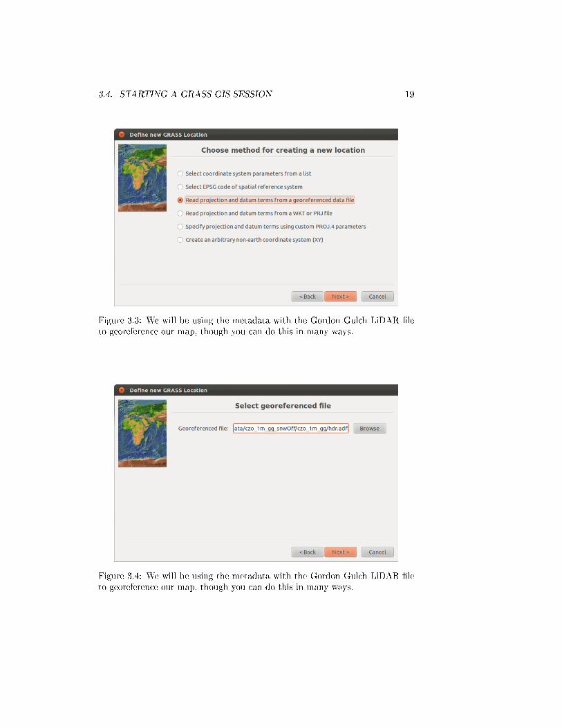
Once this folder is created, you will see a start-up screen (see Figure 3.1).Click Location Wizard. You should see a window like Figure 3.2. Set theproject location to �GordonGulch� and the location title to �Gordon Gulch -Snow O�� so the location directory on your computer matches that in thisdocumentation. Click �next�, and select the �Read projection and datum termsfrom a georeferenced data �le� option (Figure 3.3). Lots of other projectionselection methods are available, but we want to match the projection of thesample data �le, and it is easiest to just pull that out of its metadata. Click�next� and then browse to the folder where you have the Gordon Gulch datathat come with this tutorial. I usually click on the �hdr� �le (see Figure 3.4,but I think that it is smart enough to �gure it out no matter which particular�le you choose. Click �next�. You'll see a summary of your selections. Thenclick �Finish�. A window will pop up asking if you want to set the default region(Figure 3.5). Click �no� (or click �yes� and then don't change anything): theregion is the bounding box of the map and the resolution, but this has alreadybeen imported properly from the Gordon Gulch LiDAR DEM metadata. If youdo click �yes�, you will see a screen like Figure 3.6.

Now that you're done, you'll be back at the starting window, but with yournew location �GordonGulch� de�ned (Figure 3.7). Inside GordonGulch, there isa mapset called �PERMANENT�. This is the mapset that you will be using.

In collaborative projects the PERMANENT mapset typically contains onlycommunal �les, and each of you would have your own mapset created by clickingthe �create mapset� button. For example, if we were making a geologic map,a DEM, scanned USGS topo sheets, and remotely sensed data products mightbe in the PERMANENT mapset. I could read these �les, but could not writeto them or change anyone else's personal mapset. A few of us could then haveour own �contacts� vector maps that we would work on independently, withoutrisk of changing someone else's work. When we feel that we are done with ourrespective sections of the map, we could merge our maps into a �nal �contacts�vector layer, and add that to PERMANENT. This basically exists to avoidcommon �le management issues in collaborative work. The reason that we willbe each using PERMANENT as our only mapset for this tutorial should nowbe obvious: you will be the only user of your GIS location.

3.3. CREATING A LOCATION: GORDON GULCH 17

Figure 3.1: GRASS GIS start-up screen on Ubuntu. If you have just in-stalled GRASS, you will have no project locations or mapsets, and your �Createmapset�, �Rename mapset�, and �Start GRASS� buttons will be grayed out.

There is a reason and a big advantage to this initial set-up step. GRASS in-ternally manages its �le structure, and keeps all of its data inside subdirectoriesof this directory. So long as you don't add and delete �les from this directoryoutside of GRASS (unless you really know what you are doing), this keeps ev-erything very well organized: I have never had to mess with any of this. Abig advantage of this internal organization is that your GRASS directories areportable: just copy/paste the entire GRASS directory or location folder, and itwill be properly set up on another machine without any of those painful brokenlinks to data �les.

18 CHAPTER 3. STARTING GRASS AND CREATING A LOCATION

Figure 3.2: Location wizard start screen.

3.4 Starting a GRASS GIS session

Now that you've �nished setting up your location, you're ready to start usingGRASS GIS! We will each use the PERMANENT mapset, since we are the soleusers of our GIS projects and want access to everything.

Click on �Start GRASS� in the start-up window (Figure 3.7). This windowwill close, and in its place you will have 2 new GRASS windows (Figure 3.8).These are the display and the layer manager. If you have a command linewindow open as well, you should see something that looks like Figure 3.9

3.4. STARTING A GRASS GIS SESSION 19

Figure 3.3: We will be using the metadata with the Gordon Gulch LiDAR �leto georeference our map, though you can do this in many ways.

Figure 3.4: We will be using the metadata with the Gordon Gulch LiDAR �leto georeference our map, though you can do this in many ways.

20 CHAPTER 3. STARTING GRASS AND CREATING A LOCATION

Figure 3.5: You can click �no�, since the Gordon Gulck LiDAR metadata havealready properly set the computational region, which is the window that coversthe portion of the map of interest at the provided resolution. (Click �yes� to seethe parameters that can be set, but don't change them.)

Figure 3.6: If you click �yes� to edit the region (see Figure 3.5), you will get ascreen like this.

3.4. STARTING A GRASS GIS SESSION 21

Figure 3.7: Back at the start window, but all set to go.

22 CHAPTER 3. STARTING GRASS AND CREATING A LOCATION

Figure 3.8: The graphical user interface (GUI) windows in Mac OS. The right-hand window is the layer manager that is the main graphical interface forGRASS. The left-hand window is the map display.

Figure 3.9: The command line interface (CLI) in Mac.

Chapter 4

Basic Raster Display and

Region Operations

4.1 Importing GDAL Raster Data

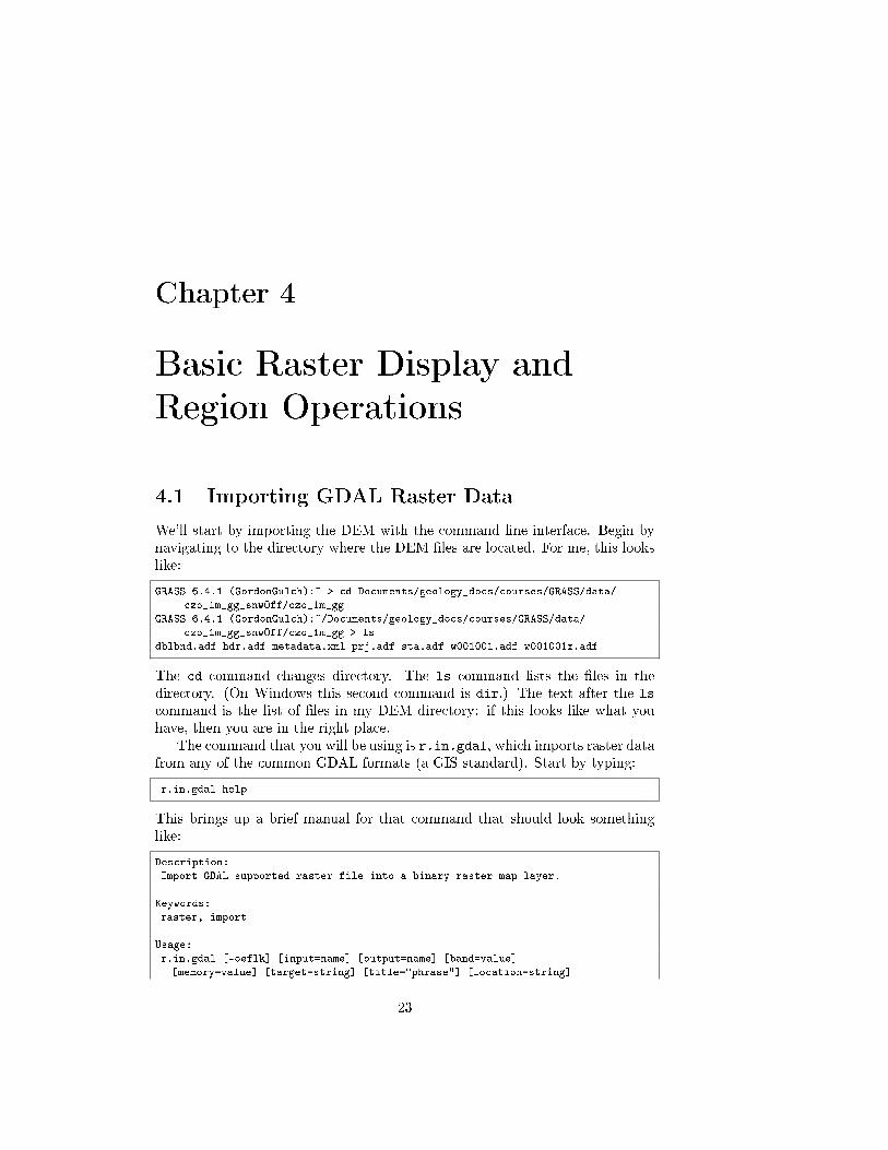
We'll start by importing the DEM with the command line interface. Begin bynavigating to the directory where the DEM �les are located. For me, this lookslike:

GRASS 6.4.1 (GordonGulch):~ > cd Documents/geology_docs/courses/GRASS/data/

czo_1m_gg_snwOff/czo_1m_gg

GRASS 6.4.1 (GordonGulch):~/Documents/geology_docs/courses/GRASS/data/

czo_1m_gg_snwOff/czo_1m_gg > ls

dblbnd.adf hdr.adf metadata.xml prj.adf sta.adf w001001.adf w001001x.adf

The cd command changes directory. The ls command lists the �les in thedirectory. (On Windows this second command is dir.) The text after the ls

command is the list of �les in my DEM directory: if this looks like what youhave, then you are in the right place.

The command that you will be using is r.in.gdal, which imports raster datafrom any of the common GDAL formats (a GIS standard). Start by typing:

r.in.gdal help

This brings up a brief manual for that command that should look somethinglike:

Description:

Import GDAL supported raster file into a binary raster map layer.

Keywords:

raster, import

Usage:

r.in.gdal [-oeflk] [input=name] [output=name] [band=value]

[memory=value] [target=string] [title="phrase"] [location=string]

23

24CHAPTER 4. BASIC RASTER DISPLAY AND REGION OPERATIONS

[--overwrite] [--verbose] [--quiet]

Flags:

-o Override projection (use location's projection)

-e Extend location extents based on new dataset

-f List supported formats and exit

-l Force Lat/Lon maps to fit into geographic coordinates (90N,S; 180E,W)

-k Keep band numbers instead of using band color names

--o Allow output files to overwrite existing files

--v Verbose module output

--q Quiet module output

Parameters:

input Raster file to be imported

output Name for output raster map

band Band to select (default is all bands)

memory Cache size (MiB)

target Name of location to read projection from for GCPs transformation

title Title for resultant raster map

location Name for new location to create

Help!Typing �help� after any command gives a summary of what it does andhow it should be used. I have been using GRASS for a long time, andI still do this fairly frequently to make sure that I am using commandscorrectly, especially when I am working in an interactive session. GRASShas a lot of features, and it can be hard to remember all of the optionsfor all of them!

Box 4.1: Help!

Our import is not going to need to use most of these commands. What wewill need to do is to type:

r.in.gdal input=hdr.adf output=topo

It is possible to shorten the names of the parameters (e.g., �input� to �in�) solong as there is no other parameter that starts with those letters. Once again,I use the hdr.adf �le, though I think that most of them should work for thisimport. Actually using this command should look something like this:

GRASS 6.4.1 (GordonGulch):~/Documents/geology_docs/courses/GRASS/data/

czo_1m_gg_snwOff/czo_1m_gg > r.in.gdal input=hdr.adf output=topo

Projection of input dataset and current location appear to match

100%

r.in.gdal complete. Raster map <topo> created.

GRASS 6.4.1 (GordonGulch):~/Documents/geology_docs/courses/GRASS/data/

czo_1m_gg_snwOff/czo_1m_gg >

This command starts with �r� because it operates on rasters. GRASS usesthese �X.� beginnings of commands to help di�erentiate the types of data onwhich they operate.

4.2. VIEWING AND SETTING THE REGION 25

UNIX/GRASS terminal syntaxSpaces separate distinct things in the UNIX terminal, so you can't havespaces around your �=� signs. In GRASS, these spaces separate inputs tothe commands. Variables are evaluated with �$�, and strings are concate-nated by doing nothing special. For example:

tmp = "testing"

d.mon x0 # open display monitor

d.rast $tmp # display "testing" raster, if it exists

d.out.file -t format=png output=$tmp_file # outputs "testing_file.png" -->

d.out.file adds the extension

Options sent to GRASS GIS commands can be shortened, if unambiguous. Forexample: �column� to �col�, �input� to �in�, �output� to �out�, ...

Flags with one hyphen can be combined (e.g., �-g -n� = �-gn�), and I typicallyput these before the main commands. I typcally put �ags with two hyphensafter commands; the most commonly-used of these is the overwrite �ag, ��o�. Ifthis �ag is not set, �les will not be overwritten.

Box 4.2: UNIX/GRASS terminal syntax

4.2 Viewing and setting the region

All of the commands that you run in GRASS are subject to a particular com-putational window, which is called the �region�. You can use the g.region

command to look at the extent of this region and modify it.

GRASS 6.4.1 (GordonGulch):~ > g.region -p

projection: 1 (UTM)

zone: 13

datum: nad83

ellipsoid: grs80

north: 4431084.5

south: 4428353.5

west: 457305.5

east: 461795.5

nsres: 1

ewres: 1

rows: 2731

cols: 4490

cells: 12262190

This command gives information on the projection type, region boundaries, andresolution. The current (and default) region is the entire area de�ned by theGordon Gulch raster that you used to de�ne the coordinate system. If youchange the region and want to bring it back to this full extent and originalresolution, type:

GRASS 6.4.1 (GordonGulch):~ > g.region rast=topo

26CHAPTER 4. BASIC RASTER DISPLAY AND REGION OPERATIONS

This sets the region to the resolution and edges of the raster �topo�.Note that this command starts with a �g�. These are the general utilities,

used for copying data sets, moving them, setting projections, and other general-purpose commands.

4.3 Displaying Raster Data

Now that we know that we have set the computational region to the full extentof the DEM, we are ready to display the data.

4.3.1 Simple raster display with the command line

We will start by viewing the raster data with the command line tool. This isn'tas nice/interactive as the GUI, but allows us to write short scripts to create andsave map images automatically. This can be nice for creating consistent �guresfor use in presentations, papers, etc.

We will do some more complex work with both the command line and GUImap displays later on, but for now we will just initialize a window and displaythe raster DEM.

d.mon start=x0 # Start X-windowing display monitor #0

r.colors map=topo color=elevation # Use the scalable elevation color scheme for

the topo map

d.rast map=topo # Display the topo map

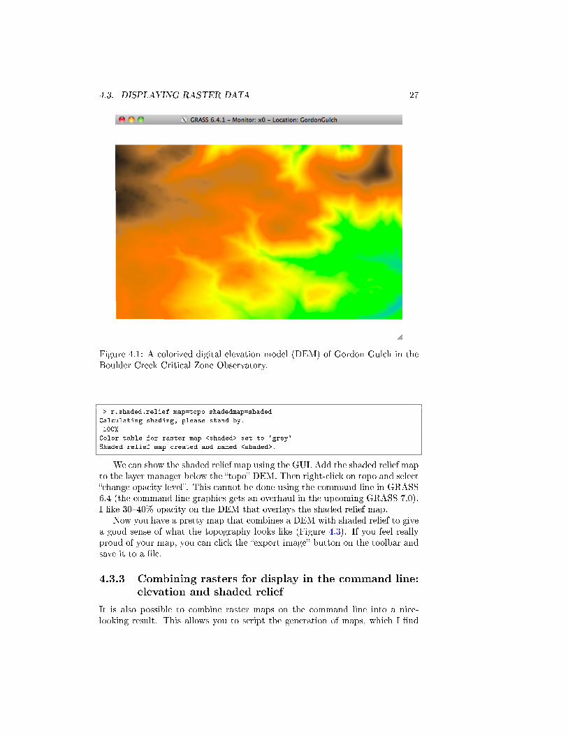
When you run these commands, you should have a window appear that lookslike Figure 4.1.

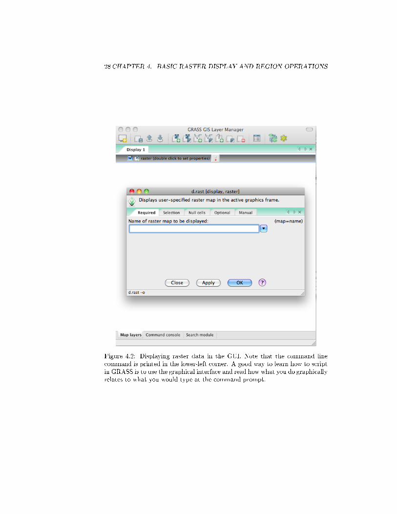
4.3.2 Displaying raster (elevation and shaded relief) mapsin the graphical interface

We can do the same thing in the graphical interface. In the �GRASS GIS LayerManager� window, click on the icon with the checkerboard grid and the plus signin the top bar. This is the raster display button. A window will appear as soonas you click it (Figure 4.2). There should be only one map in the drop downlist, our �topo�. Select it and hit �OK�. You should now see the LiDAR DEMdisplayed a second time. If it isn't showing up correctly, you might have to hitthe �zoom to computational region� button on the GRASS GIS Map Displaythat goes along with the GUI.

Now, let's add a shaded relief map. Since we have not yet executed anycommands other than the map display with the graphical interface, we willuse that to construct the shaded relief map. On the menu bar, click Raster→ Terrain analysis → Shaded relief. The input elevation map should be�topo�. Under the �optional� tab, set the output shaded relief map name to�shaded�. Click �Run�.

This is equivalent to running the following on the command line:

4.3. DISPLAYING RASTER DATA 27

Figure 4.1: A colorized digital elevation model (DEM) of Gordon Gulch in theBoulder Creek Critical Zone Observatory.

> r.shaded.relief map=topo shadedmap=shaded

Calculating shading, please stand by.

100%

Color table for raster map <shaded> set to 'grey'

Shaded relief map created and named <shaded>.

We can show the shaded relief map using the GUI. Add the shaded relief mapto the layer manager below the �topo� DEM. Then right-click on topo and select�change opacity level�. This cannot be done using the command line in GRASS6.4 (the command line graphics gets an overhaul in the upcoming GRASS 7.0).I like 30�40% opacity on the DEM that overlays the shaded relief map.

Now you have a pretty map that combines a DEM with shaded relief to givea good sense of what the topography looks like (Figure 4.3). If you feel reallyproud of your map, you can click the �export image� button on the toolbar andsave it to a �le.

4.3.3 Combining rasters for display in the command line:elevation and shaded relief

It is also possible to combine raster maps on the command line into a nice-looking result. This allows you to script the generation of maps, which I �nd

28CHAPTER 4. BASIC RASTER DISPLAY AND REGION OPERATIONS

Figure 4.2: Displaying raster data in the GUI. Note that the command linecommand is printed in the lower-left corner. A good way to learn how to scriptin GRASS is to use the graphical interface and read how what you do graphicallyrelates to what you would type at the command prompt.

4.3. DISPLAYING RASTER DATA 29

Figure 4.3: The gorgeous Gordon Gulch!

especially useful for time-series of data.I use r.blend so I can export the resultant set of rasters later on in this

tutorial. Another command, d.shadedmap, works well for draping maps overone another in the display monitor without creating any new rasters. Whileyou can't export the raster directly from the display window, you can also used.save, d.out.file, and other commands to save an image of the currentdisplay.

# Blend two rasters into a nice result!

r.blend first=topo second=shaded output=colored_shaded_relief percent=40

# This creates a RGB triplet for the shaded relief map that you can display

d.mon x0

d.rgb r=colored_shaded_relief.r g=colored_shaded_relief.g b=colored_shaded_relief

.b

# We can use commands to add a title and other nifty features too!

# d.title is used to display the map title and other info; this is

# in the map's metadata.

# d.text adds selected text

# There are lots of d.* commands to choose from!

30CHAPTER 4. BASIC RASTER DISPLAY AND REGION OPERATIONS

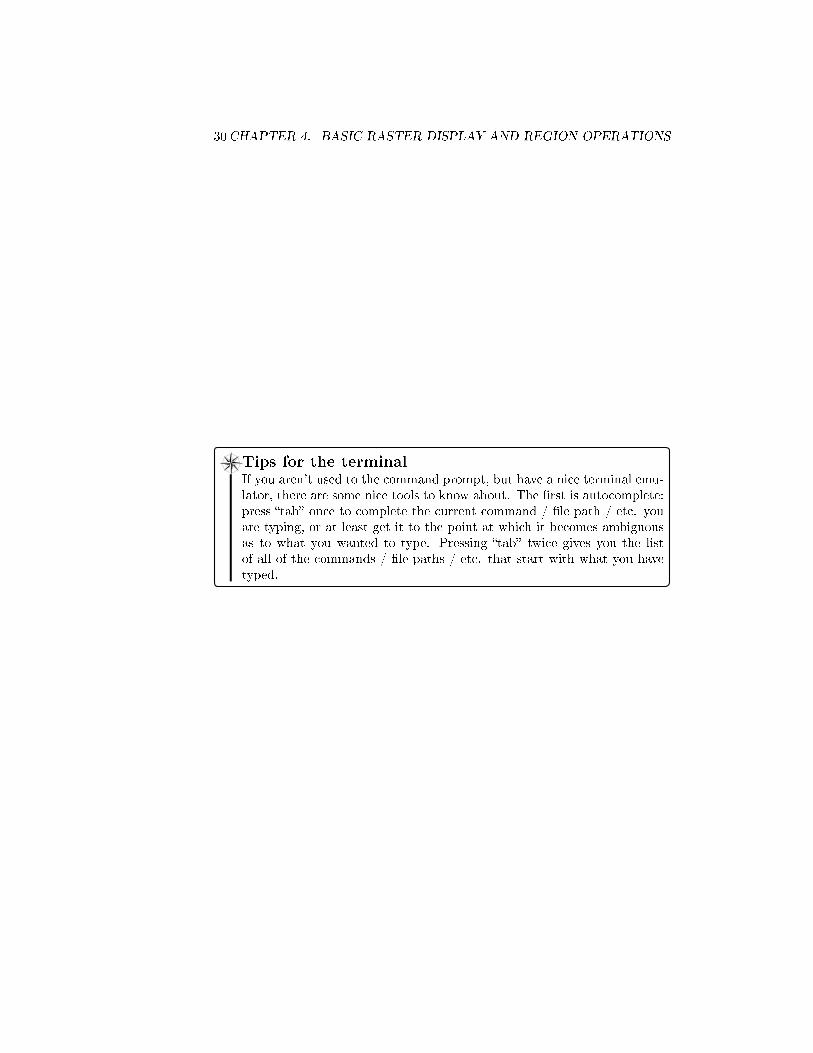
Tips for the terminalIf you aren't used to the command prompt, but have a nice terminal emu-lator, there are some nice tools to know about. The �rst is autocomplete:press �tab� once to complete the current command / �le path / etc. youare typing, or at least get it to the point at which it becomes ambiguousas to what you wanted to type. Pressing �tab� twice gives you the listof all of the commands / �le paths / etc. that start with what you havetyped.

Box 4.3: Tips for the terminal

Chapter 5

Topographic and hydrologic

analyses

5.1 Slope, aspect, and resampling

Let's try another example using the graphical interface (GUI) instead of thecommand line. We will measure slope and aspect.

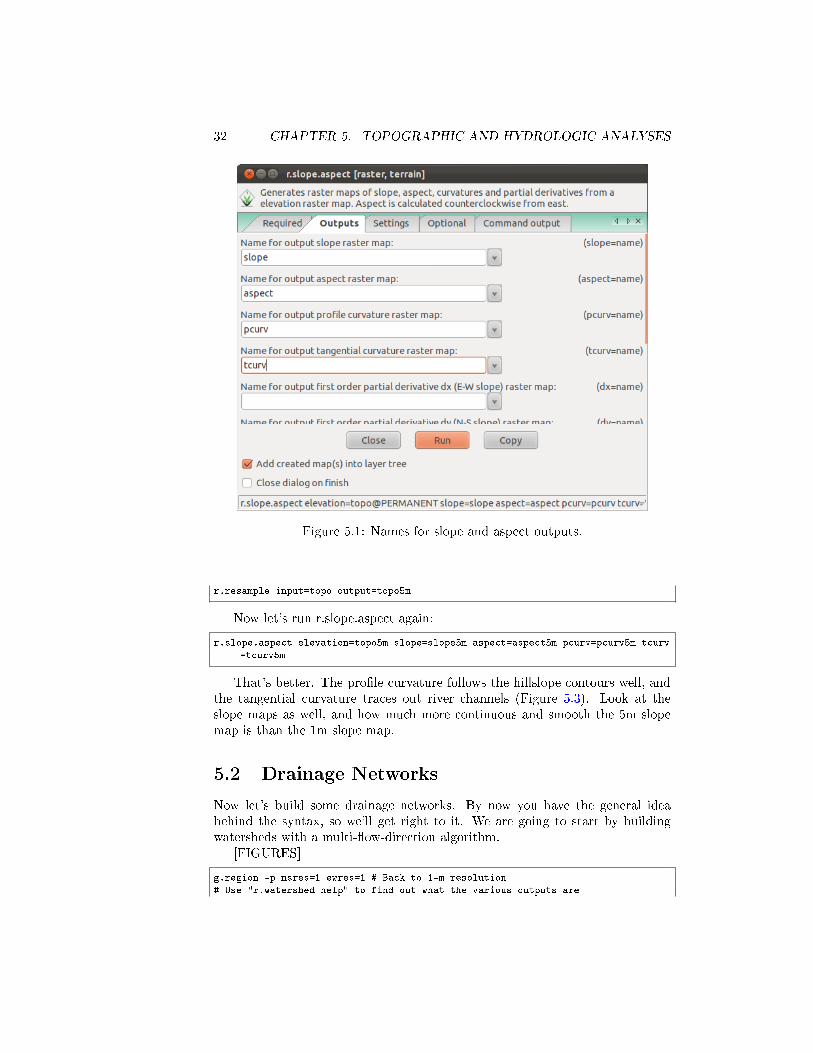
Go to the Raster menu. Raster → Terrain analysis → Slope and as-pect. Set the raster map to "topo", then click the "outputs" tab. We won'tcalculate x- and y- derivatives, as these are in an arbitrary orientation withrespect to the hills and valleys. We instead will calculate the slope (steepestdecent), aspect, pro�le (steepest descent orientation) curvature, and tangen-tial (shallowest descent orientation) curvature. I call these "slope", "aspect","pcurv", and "tcurv", respectively. (See Figure 5.1.) Look at the bottom. Thecommand-line output is given here. This means that by entering values in theGUI, you can teach yourself how to use the command line � which is very niceas you start to want to write pre-packaged analysis algorithms. With the GUIwindow for r.slope.aspect selected, press CTRL+c (or Command+c on mac �actually, I can't get this to work on mac), and you copy this command-linestring:

r.slope.aspect elevation=topo slope=slope aspect=aspect pcurv=pcurv tcurv=tcurv

Click "run" and it prints out this command line string and runs the desiredcommand.

Try displaying one of the curvature maps in the viewer. It looks like abunch of random noise (Figure 5.2). This is because of the high (1 meter)resolution of the LiDAR data: tiny bumps on the surface are dominating thesignal. Let's resample these data to 5 meter resolution. First, we have tochange our computational region's resolution. Then we use the "r.resample"tool to coarsen our raster map.

g.region -p nsres=5 ewres=5 # "-p" prints the computational window.

31

32 CHAPTER 5. TOPOGRAPHIC AND HYDROLOGIC ANALYSES

Figure 5.1: Names for slope and aspect outputs.

r.resample input=topo output=topo5m

Now let's run r.slope.aspect again:

r.slope.aspect elevation=topo5m slope=slope5m aspect=aspect5m pcurv=pcurv5m tcurv

=tcurv5m

That's better. The pro�le curvature follows the hillslope contours well, andthe tangential curvature traces out river channels (Figure 5.3). Look at theslope maps as well, and how much more continuous and smooth the 5m slopemap is than the 1m slope map.

5.2 Drainage Networks

Now let's build some drainage networks. By now you have the general ideabehind the syntax, so we'll get right to it. We are going to start by buildingwatersheds with a multi-�ow-direction algorithm.

[FIGURES]

g.region -p nsres=1 ewres=1 # Back to 1-m resolution

# Use "r.watershed help" to find out what the various outputs are

5.2. DRAINAGE NETWORKS 33

Figure 5.2: At 1 meter resolution, local topographic variations completely dom-inate the curvature signal, removing any obvious signal of the larger-scale land-scape.

GRASS GIS online (and o�ine) helpTo learn about the multi-�ow-direction algorithm, or most of the otheralgorithms in GRASS, you can go to their help page. Look at the mainGUI window (the one that shows the layers in display or the commandline). On its toolbar, click on the rescue ring; this opens a browserwindow with the GRASS help.

The GRASS help index tells you how to use the commands and whatresearch, theories, and/or publications the commands implement. Thishelp often comes with examples and/or diagrams to better explain thesituations.

In this particular case, we will navigate to the raster command index andlook for r.watershed, a watershed basin creation program. [NEW REF]

Box 5.1: GRASS GIS online (and o�ine) help

# We are using multi-direction flow; you can use single-direction ("SFD")

# by removing the "-f" flag

# Threshold=62500 means that we need an accumulation area > 250x250 cells

# = 250x250 meters here

r.watershed -f elevation=topo accumulation=accum_mfd drainage=draindir_mfd basin=

basins_mfd stream=streams_mfd threshold=62500

34 CHAPTER 5. TOPOGRAPHIC AND HYDROLOGIC ANALYSES

Figure 5.3: At 5 meter resolution, the tangential curvature is still noisy, butchannel networks have become visuallly discernable.

# Thin the channels raster so we can vectorize it

r.thin input=streams_mfd output=streams_mfd_thinned

# And to vector of stream channels

# Vector and raster datasets may have the same name without overwriting each

other.

r.to.vect input=streams_mfd_thinned output=streams_mfd

# Now to vectorize drainage basins

r.to.vect input=basins_mfd output=basins_mfd feature=area

The �thinning� step ensures that there are no clumps of pixels, and that asingle vector line therefore can be drawn cleanly through the raster during ther.to.vect step.

GRASS add-onsGRASS GIS has a number of add-ons. These are applications that havenot been fully adopted and integrated into the GRASS suite of tools, butthat can still be very useful. One of these, r.stream, is used for thekinds of watershed problems that we are tackling right now. We will beusing the built-in GRASS tools in this tutorial, but to learn more aboutthe GRASS add-ons, go to their wiki page: http://grass.osgeo.org/

wiki/GRASS_AddOns.

Box 5.2: GRASS add-ons

While the multiple �ow direction algorithm is good for providing a more

5.3. GORDON GULCH DRAINAGE BASIN FROM SET POUR POINT 35

accurate representation of �ow paths, single �ow direction is needed for streampro�ling. We are also going to relax the threshold drainage area down to 10,000cells (10,000 m2 = 100x100 meters). Let's do that now.

r.watershed elevation=topo accumulation=accum drainage=draindir basin=basins

stream=streams threshold=10000

r.thin input=streams output=streams_thinned

r.to.vect input=streams_thinned output=streams

r.to.vect input=basins output=basins feature=area

Now we have a set of single vector stream lines in the basin, each of whichrepresents a segment of the full river channel.

Where I have been using the threshold, I have been doing so in terms ofcells. But if your cell sizes vary, or you want to input real �ow contributionsfrom each cell, you can do that by setting the flow parameter in r.watershed

to the name of a raster map.Let's cap our calculatory achievments by displaying the SFD streams on top

of the color shaded relief via the command line:

d.mon x0

# d.vect -c map=basins_mfd type=boundary # These get confusing, but this is how

to display area boundaries

d.rgb r=colored_shaded_relief.r g=colored_shaded_relief.g b=colored_shaded_relief

.b

d.vect map=streams color=blue

5.3 Gordon Gulch drainage basin from set pourpoint

We can use the GRASS r.water.outlet function to build basins from pourpoints. In the next exercise, we will do that, along with vectorizing the resultantdrainage basin.

A pour point is the selected map location from which to calculate the up-stream catchment area. This is given by the easting and northing values,which I have typed here to be the outlet of Gordon Gulch, thus making us �ndthe largest basin on the map.

When we vectorize the drainage basin area, note that we have to clean thetopology by removing small (1-pixel) areas that are created along with the largedrainage basin. This sometimes happens when converting from raster to vector.I use v.clean, a topology cleaning tool, to remove these small areas. If thereare small areas without centroids like these that you would actually want tokeep, you can try to add centroids to them with the v.centroids tool.

# Gordon Gulch basin. Output: 1=inside basin; 0=outside basin

r.water.outlet easting=461795 northing=4429173 drainage=draindir basin=GGbasin

# Set non-basin cells to NULL

r.null map=GGbasin setnull=0

# Convert raster to vector: Use the "-s" flag if you want to smooth the vector

instead

36 CHAPTER 5. TOPOGRAPHIC AND HYDROLOGIC ANALYSES

# of having rectangular pixel-shaped edges

r.to.vect in=GGbasin out=GGbasin feature=area

# What? 4 areas created? But only 1 centroid?

# Need to clean topology after raster conversion. All of the areas without

# centroids are just one pixel, so we will use v.clean:

v.clean in=GGbasin out=tmp tool=rmarea thresh=1 --o

# And now we will copy over our GGbasin vector file and remove "tmp",

# all in one fell swoop, with "rename":

g.rename vect=tmp,GGbasin --o

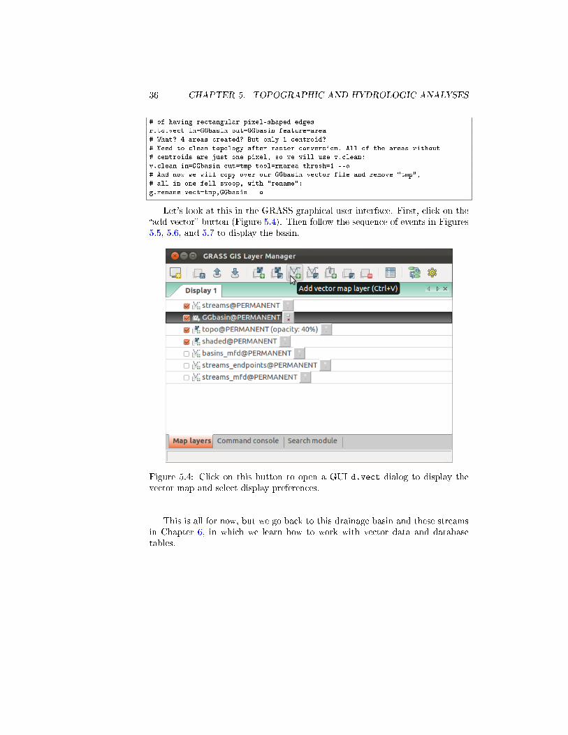
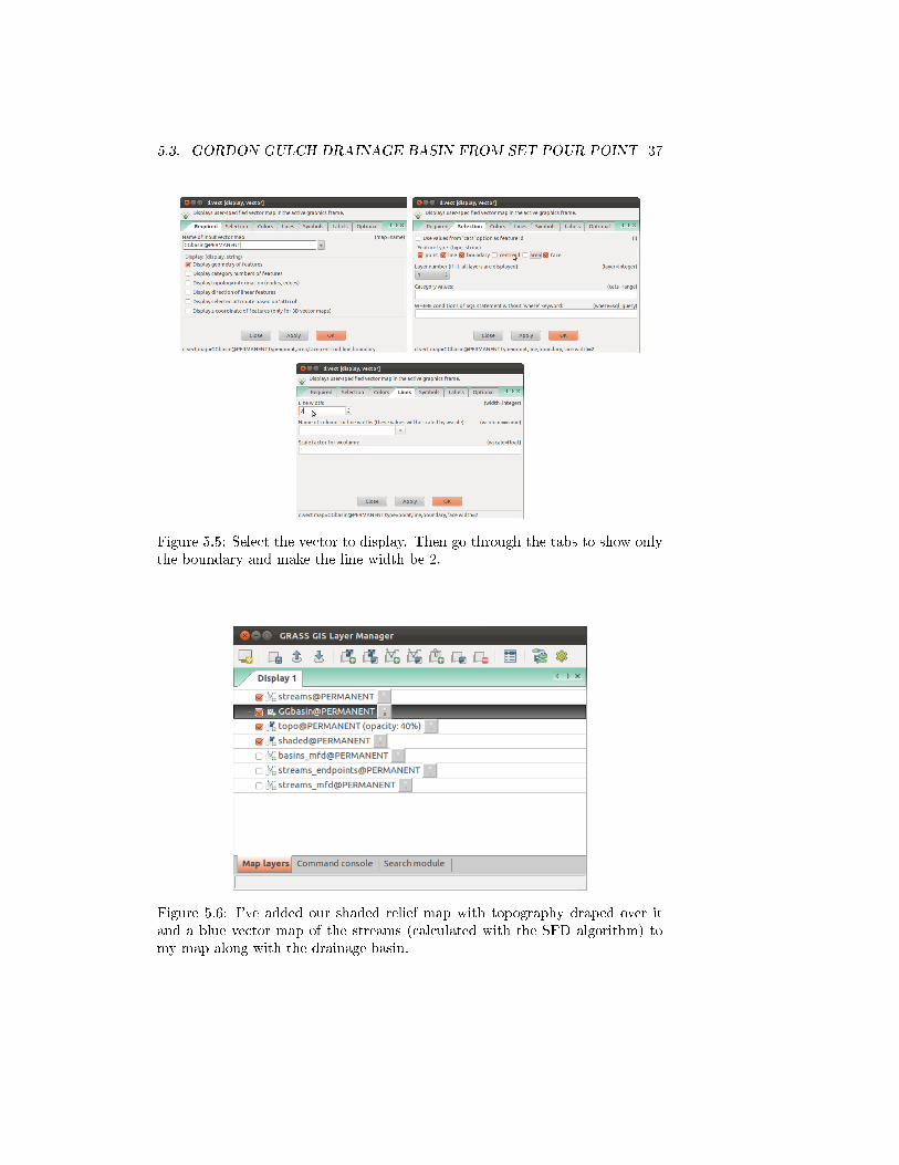
Let's look at this in the GRASS graphical user interface. First, click on the�add vector� button (Figure 5.4). Then follow the sequence of events in Figures5.5, 5.6, and 5.7 to display the basin.

Figure 5.4: Click on this button to open a GUI d.vect dialog to display thevector map and select display preferences.

This is all for now, but we go back to this drainage basin and these streamsin Chapter 6, in which we learn how to work with vector data and databasetables.

5.3. GORDON GULCH DRAINAGE BASIN FROM SET POUR POINT 37

Figure 5.5: Select the vector to display. Then go through the tabs to show onlythe boundary and make the line width be 2.

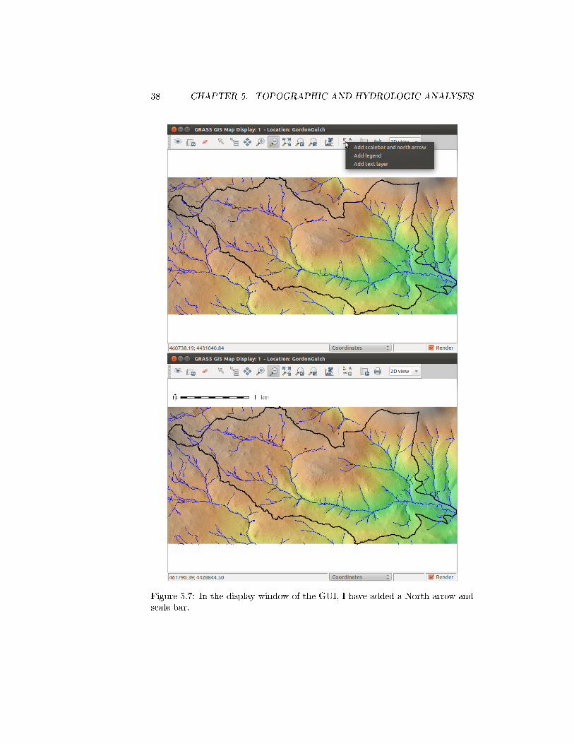
Figure 5.6: I've added our shaded relief map with topography draped over itand a blue vector map of the streams (calculated with the SFD algorithm) tomy map along with the drainage basin.

38 CHAPTER 5. TOPOGRAPHIC AND HYDROLOGIC ANALYSES

Figure 5.7: In the display window of the GUI, I have added a North arrow andscale bar.

5.4. SOLAR RADIATION 39

5.4 Solar radiation

Another important topographic analysis is solar radiation. GRASS GIS has ar.sun module that does just this, with all the bells and whistles (direct, di�use,and re�ected radiation, variable surface albedo, atmospheric conditions, etc.)

You will need to have run r.slope.aspect to get the slope and aspect indecimal degrees as inputs to the solar radiation �le (Section 5.1).

The following is an example of r.sun usage. I haven't used it too much,so I don't have too much to say about it, but it looks pretty powerful. Thehelp page (http://grass.fbk.eu/gdp/html_grass64/r.sun.html for GRASS6.4.X) gives a pretty thorough description of it, as well as a nice bibliographyof the literature (largely solar energy papers) from which the r.sun developersdrew. The GRASS wiki page has more information: http://grass.osgeo.

org/wiki/R.sun. I've thought about linking it in with measured temperaturedata: r.sun could help to obtain the upper boundary heat �ux, and could be away towards obtaining a realistic distributed thermal history for a region thathas limited point measurements.

# lat~40, but we don't need this: GRASS knows where we are

# This process may take several minutes, especially when you are running it for a

whole day!

r.sun -s elevin=topo aspin=aspect slopein=slope day=28 beam_rad=

beam_irradiation_day insol_time=insolation_time_day diff_rad=

diffuse_irradiation_day refl_rad=reflected_irradiation_day

# Let's sum all of the three radiation types for the whole-day option, using the

map calculatior:

r.mapcalc "total_irradiation_day28 = beam_irradiation_day +

diffuse_irradiation_day + reflected_irradiation_day"

# Given time - segfaults as with 6.4.1: fixed in newer versions (6.4.2 might be

release version now, so we could be safe on this)

# Segfault also caused by including latitude as either value or raster

r.sun -s elevin=topo aspin=aspect slopein=slope lat=40 day=28 time=8.0 beam_rad=

beam_irradiance_0800 diff_rad=diffuse_irradiance_0800 refl_rad=

reflected_irradiance_0800

As a quick review of plotting with the addition of a legend, and an earlyintroduction to Bash scripting (Section 8.2) and �le I/O (Chapter 7), I amgoing to run the following script to display and save images of all of the timesteps. I am also using a number of plotting bells and whistles as an example oftheir usage. The output is given in Figure 5.8

d.mon x1 # start display monitor

# start a for loop

for radrast in beam_irradiation_day diffuse_irradiation_day

reflected_irradiation_day total_irradiation_day28

do

# "echo" is Bash's cute way of saying "print this to an output"; by default,

stdout = terminal window

# "$" in Bash indicates that a variable should be evaluated; otherwise, it is

treated as itself

# (e.g., radrast = radrast; $radrast = beam_irradiation_day)

40 CHAPTER 5. TOPOGRAPHIC AND HYDROLOGIC ANALYSES

echo $radrast

d.rast $radrast

d.title -ds map=$radrast

d.grid -gw size="0:01" color=white textcolor=black fontsize=16

d.legend map=$radrast color=black at=15,85,15,18

d.barscale bcolor=none at=0,93

# save the image here

d.out.file -t output=$radrast format=png --o

sleep 1 # Take a look at it!

d.erase

done

Figure 5.8: Solar radiation maps for January 28th. Some of the features in thestandard GRASS output, like the grid and legend text, are thin and don't showup well in this multi-color �gure. This is a weakness of the GRASS automateddisplays.

5.5 Cosmogenic dating

One of the many things on my long to-do list is to create a GRASS GIS programto obtain cosmogenic production rates. While I havne't even started coding this,I'll say a little here about how I would do this in GRASS.

GRASS has a function called r.horizon. It gets the elevation of the horizonfrom around a point on a DEM. This, coupled the elevation of the sample and

5.5. COSMOGENIC DATING 41

an atmospheric thickness function, should be able to give a production rate witha global-uniform assumption. The point also has an (x, y) position. From this,any spatial variability in cosmogenic production rates should be calculatable.

42 CHAPTER 5. TOPOGRAPHIC AND HYDROLOGIC ANALYSES

Chapter 6

Vectors and databases

6.1 Vector topology

In GRASS GIS, an �area� comprises a �boundary��a line that encloses it�and a�centroid��a point within the area that shows on which side of the line the areaexists. Vector attributes for areas are attached to the centroids of these areas.Boundaries are shared between areas, and have their own set of attributes: theyknow about the areas on either side of them, their lengths, etc.

This is a �topological� paradigm for vector �les that prevents the sliversand overlaps in vector �les that are common in shape�les. (I think that Ar-c/Info had topologically correct features, but ArcDesktop stopped doing that,possibly to make our lives more di�cult...) Anyway, Figure 6.1 shows the di�er-ences between shape�les and the topological vectors that GRASS uses. The �g-ures are from the GRASS Wiki, http://grass.osgeo.org/wiki/Digitizing_Area_Features; this page has more information on vector topology.

Figure 6.1: GRASS maintains vector topology, with shared boundaries betweenareas and individual areas de�ned by centroids. Figures from GRASS Wiki,http://grass.osgeo.org/wiki/Digitizing_Area_Features.

43

44 CHAPTER 6. VECTORS AND DATABASES

Other aspects of GRASS vector topology are that points cannot overlap, andlines should not cross or overlap. The whole point of this is to make sure thatthere are not redundancies or ambiguities in the vecto data: careful preparationof vector data sets can be hugely important for data processing and interpreta-tion!

6.2 Managing databases and uploading vector at-tributes

We will learn how to manage vector databases with the GGbasin vector createdin Section 5.3. This vector has only 1 area and no shared boundaries, so it isthe simplest possible starting point (aside from, well, a point).

My most-commonly used command is v.db.select. This command printsthe database values to the screen (or a �le), and optionally �lters them accordingto a SQL queery. Try it out! When I do, this happens:

GRASS 6.4.1 (GordonGulch):~/grasstmp > v.db.select GGbasin

cat|value|label

1|1|

The category, �cat�, is a unique ID for each vector feature that starts at 1and goes upward. �Value� is 1 from the conversion from raster. �Label� is empty,because there was no label attached to the drainage basin raster.

Let's add the area of the drainage basin. To do this, we need to add acolumn:

v.db.addcol map=GGbasin columns="area double precision"

Check it out: a new column is here!

GRASS 6.4.1 (GordonGulch):~/grasstmp > v.db.select GGbasin

cat|value|label|area

1|1||

Columns can be �double precision�, �int�, �varchar�, or �date�. Other typesexist as well, depending on the database manager being used, but I have neverhad to use anything but the �rst three mentioned here.

To put a real value in this column, we must get the vector attribute (knownbut hidden) into the database table. This uses the command v.to.db. Makessense, huh? Vector to database! I choose �units=k� for km2.

GRASS 6.4.1 (GordonGulch):~/grasstmp > v.to.db map=GGbasin opt=area columns=area

units=k

Reading areas...

100%

Updating database...

100%

1 categories read from vector map (layer 1)

1 records selected from table (layer 1)

1 categories read from vector map exist in selection from table

1 records updated/inserted (layer 1)

6.3. ADVANCED VECTOR AND DATABASE PROCESSING 45

GRASS 6.4.1 (GordonGulch):~/grasstmp > v.db.select GGbasincat|value|label|area

1|1||4.195303

There we go! This can be used to �nd neighbors, line slopes, perimeters,and lots more fun stu�. Something I've thought about is writing a slope-areacalculation algorithm for a whole landscape... would be very do-able, but I justhaven't done it yet!

6.3 Advanced Vector and Database Processing

I thought about subtitling this section Streams (lines), Stream SegmentEndpoints (points), and Drainage Basins (areas). It could also be sub-titled Manipulating Lines and Points, Using Databases, and File I/O.So this may make it sound like a mixed bag, but it will make sense when it isall done. The point of it is that we can do a lot of nifty stu� with lines, whatwe've just learned about getting attribute values, and some basin piping of out-put to extract drainage basins and/or get some pretty interesting landscapecharacteristics.

6.3.1 Obtaining and cleaning points in stream networks

Back in Section 5.2, we created a set of vector lines for streams. Each of thelines in this vector extends between the two nearest next tributary junctions,the start of the river system (determined by the drainage threshold we selected),and/or the edge of the map.

We can extract points from this vector using the v.to.points function. Inthis case, I am setting the -n �ag to look just at the nodes (endpoints) of thelines. The -v command would get all of the vertices of the line, and -i wouldinterpolate between these vertices.

v.to.points -n input=streams output=streams_endpoints

# Multiple points at tributary junctions: let's clean the topology

v.clean in=streams_endpoints out=tmp tool=rmdupl

# The current attribute tables do not represent our cleaned vector, so let's drop

them

v.db.droptable -f map=tmp layer=1

v.db.droptable -f map=tmp layer=2

# We also caused categories to merge by removing duplicate points; let's

# regenerate them in a nice, sequential list

v.category in=tmp out=tmp2 opt=del --o

v.category in=tmp2 out=tmp opt=add --o

# And now we'll regenerate a new table with our new categories

v.db.addtable map=tmp # Adds a table with just the default "cat" column

# Now that we're done, we will overwrite the input file

g.copy vect=tmp,streams_endpoints --o

I will now add the positions of those points with v.to.db, as well as theirelevations via queerying the raster map with v.what.rast. (Getting their lo-cations probably won't be necessary, but it's good practice; note also that you

46 CHAPTER 6. VECTORS AND DATABASES

can use v.to.db to get the start and end points of lines directly, in a databasetable that is attached to those lines. Cool, huh?)

v.db.addcol map=streams_endpoints columns="x double precision, y double precision

, z double precision"

v.to.db map=streams_endpoints col=x,y units=meters option=coor

v.what.rast vect=streams_endpoints rast=topo col=z

# Run a quick v.db.select to check on your handiwork

v.db.select streams_endpoints

Some vector �les (not this one) have z-coordinates attached as well, meaningthat we could skip the v.what.rast step and just use col=x,y,z.

6.3.2 Queerying categories

Let's say we want to �nd only the point that we used to de�ne the major basinof Gordon Gulch. This point should have the lowest of all of the values in ourvector categories�and indeed should likely have the lowest elevation of all thepoints on the map.

Doing this requires making database queeries. Remember Section 3.2, wayback up top? This is where that becomes important. We de�ned our databasemanager as SQLite, which is a useful subset of SQL (�Structured Queery Lan-guage�), pronounced �sequel�. Honestly, I �nd SQL to be a total pain, but onceyou understand its (rigid) structure and that it is better than the normal set ofdatabase managers out there, you start to put up with it and use it.

SQL can be used to perform queeries. For example, to �nd the minimumelevation from the set of stream endpoints and assign it to variable �zmin�, Itype:

zmin=`echo "SELECT MIN(z) from streams_endpoints" | db.select -c`

# Without the "-c" flag, we would need this to cut off the column name:

# zmin=${zmin:7:${#zmin}} #

Now that we have this value, we can �nd the column that is associated withthis and save its x and y coordinates.

# First, print it all

echo "SELECT * from streams_endpoints WHERE z=$zmin" | db.select

# Then save the latitude and longitude

GGx=`echo "SELECT x from streams_endpoints WHERE z=$zmin" | db.select -c`

GGy=`echo "SELECT y from streams_endpoints WHERE z=$zmin" | db.select -c`

The commands with pattern db.* are the purely-databse-oriented queeries.We can't do this �x = MIN(x)� queery in a single step because a SQL com-

mand that returns a single value like MIN() can't be used to queery wholecolumns. See - sort of a pain! This is one way in which the GRASS Pythoninterface becomes useful: vector data can be ingested as lists, which are waaaaymore �exible and a lot less painful to use. But let's keep in 100% GRASS +Bash to do the rest for now.

Now we can build our watershed from before using entirely vector outputs,without having to pick (by hand) these values.

6.3. ADVANCED VECTOR AND DATABASE PROCESSING 47

r.water.outlet easting=$GGx northing=$GGy drainage=draindir basin=GGbasinVARxy

... but if you go to display this raster, you'll �nd out that it is NOT ourbig basin! We are looking at a small enough area that the normal assumptionthat the biggest basin's outlet will have the lowest elevation won't always hold.Interesting!

6.3.3 Extracting vector subsets

Let's use our big basin vector to extract only those streams that are within it.We use v.select for this.

v.select ainput=streams binput=GGbasin operator=overlap output=GGstreams

Other useful commands that are like this are v.overlay, which combines(overlays) two vector maps, and v.extract, which extracts a subset of a vectormap based on database queeries.

The output of this command can be produced in the display window (Figure6.2):

d.mon x0

d.shadedmap reliefmap=shaded drapemap=topo brighten=15

d.vect map=GGstreams color=blue

d.vect map=GGbasin color=black type=boundary width=2

d.text -b size=8 text="Gordon Gulch Drainage" color=black font=romanc

d.barscale bcolor=none at=0,93

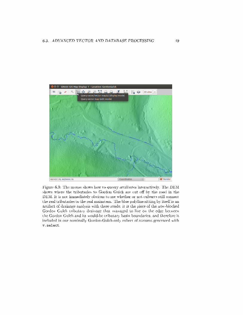
On viewing this, you might notice two tributaries that should �ow into thedownstream end of Gordon Gulch but don't: this is because of the road thatappears in the LiDAR. Look for it when you zoom in. Note that a segment ofthe �stream� along the road ended up in the Gordon Gulch drainage by mistake!We have to �x that. On the GUI, click the Queery command (Figure 6.3, selecteither �display mode� (will be displayed in the GRASS terminal tab of yourlayers, etc. window) or �edit� mode (will show up in a pop-up window), selectthe �GGstreams� layer, and click on that segment. On my computer, this returnscat:788. We want to get rid of this, so we use v.extract with the -r �ag toinvert our selection:

g.copy vect=GGstreams,GGstreams_pre_fix # make a backup first

v.extract -r in=GGstreams_pre_fix out=GGstreams where="cat=788" --o

Voilà: it's gone!Now that you have just the streams inside this area, you should be able to

use them to generate slope-area relations, to compare with �eld data, and toextract long pro�les from their starting points. We have seen that GRASS iscapable of all of these things on its own, but because of the clunkiness of SQL,it may not be the easest way to do it. Therefore, I prefer to run these types ofanalyses in Python (Section 8.3).

48 CHAPTER 6. VECTORS AND DATABASES

Figure 6.2: Drainage from Gordon Gulch only.

Specifying pour point locations by intersectionsYou often want to know the draiange area above a point given by theintersection of the stream and another linear feature (a road, a terracesurface edge that is being incised, etc.). There is a neat little trick todo this that is described in a few places online. The basic idea is tocombine the vector line �les and then use the topology tool v.clean to�nd intersections between lines, and have its �error� output be pointsthat give the intersection locations. We then use these input positions asvariable inputs to r.water.outlet, with the help of a little scripting andpiping (see the GRASS Wiki link below and Section 8.2). Nifty! This isdescribed online in the following places:

� http://grass.osgeo.org/wiki/Creating_watersheds

� http://www.surfaces.co.il/?p=241

Box 6.1: Specifying pour point locations by intersections

6.3. ADVANCED VECTOR AND DATABASE PROCESSING 49

Figure 6.3: The mouse shows how to queery attributes interactively. The DEMshows where the tributaries to Gordon Gulch are cut o� by the road in theDEM. It is not immediately obvious to me whether or not culverts still connectthe real tributaries to the real mainstem. The blue polyline sitting by itself is anartifact of drainage analysis with these roads: it is the piece of the now-blockedGordon Gulch tributary drainage that managed to live on the edge betweenthe Gordon Gulch and its would-be tributary basin boundaries, and therefore isincluded in our nominally Gordon-Gulch-only subset of streams generated withv.select.

50 CHAPTER 6. VECTORS AND DATABASES

Chapter 7

File input and output

File input and output is handled through a number of modules, depending onthe types of data and/or output desired.

7.1 Raster

At the very beginning of this manual (Section 4.1), we imported raster datawith r.in.gdal. This allows us to import any of the GDAL compatible rasterformats. r.in.ascii allows import of ASCII grids with GRASS headers. Thereare a lot of input and output commands based on this same r.in.* or r.out.* pattern, and they work for everything from SRTM data and ArcGIS gridsto Matlab *.mat �les to POV-RAY raytraceable �les to images (and lots in-between).

GRASS 6.4.1 (GordonGulch):~ > r.in.

r.in.arc r.in.bin r.in.mat r.in.wms

r.in.ascii r.in.gdal r.in.poly r.in.xyz

r.in.aster r.in.gridatb r.in.srtm

GRASS 6.4.1 (GordonGulch):~ > r.out.

r.out.arc r.out.gdal.sh r.out.png r.out.tiff

r.out.ascii r.out.gridatb r.out.pov r.out.vrml

r.out.bin r.out.mat r.out.ppm r.out.vtk

r.out.gdal r.out.mpeg r.out.ppm3 r.out.xyz

We will practice �le input and output with the raster maps from Section4.3.3. If we want to export these data to a �le, we need to �group� the .r, .g,and .b components together. For this, we use the �group� command, which isin the i.* image processing command set.

i.group group=colored_shaded_relief input=colored_shaded_relief.r,

colored_shaded_relief.g,colored_shaded_relief.b

Now we can export an image of the raster to a �le. I like PNG for imagesbecause it can have transparency.

r.out.gdal in=colored_shaded_relief out=colored_shaded_relief.PNG format=PNG

51

52 CHAPTER 7. FILE INPUT AND OUTPUT

Image processingA large component of GIS work deals with image processing. Grass hasa large set of image processing commands that are listed as i.*. Theylook pretty nifty to me, but I've never had need to use them. The sameprinciples of GRASS scripting that we have discussed so far apply to thesecommands.

Box 7.1: Image processing

Note the message in which the precision of the output is changed to match whatPNG can handle.

Let's also output a real GIS format. You can type:

r.out.gdal -l

to get a list of all available formats.Let's try an Erdas Imagine Image (.img):

r.out.gdal in=colored_shaded_relief out=colored_shaded_relief.img format=HFA

Finally, let's try to export an ASCII �le:

r.out.ascii in=colored_shaded_relief out=colored_shaded_relief.txt

Wait a minute: that didn't work! GRASS just told us:

ERROR: Raster map <colored_shaded_relief> not found

3-channel data can be stored in GDAL formats, but not in a single ASCII �le.We don't have any raster that is called colored_shaded_relief: all we haveis the group that comprises the (r,g,b) triplet. All right - let's just export ourall-day solar intensity map instead:

r.out.ascii in=total_irradiation_day28 out=total_irradiation_day28.txt

Now that works. Note that r.out.ascii tends to take longer and make bigger�les. ASCII is the easiest and most universal to read, but is usually also thelargest and clunkiest �letype.

This ASCII �le has a GRASS header, allowing it to be read back in andproviding georeferencing information. This header can be left out if you chosethe �-h� �ag. For the groundwater modelers, a �-m� �ag writes a MODFLOW-compatible grid.

We'll skip �le input, but at this point, you know how the syntax shouldwork.

7.2 Vector

Vector I/O works in the same way as raster I/O. The vector I/O commands are:

7.3. GOOGLE EARTH 53

GRASS 6.4.1 (GordonGulch):~ > v.in.

v.in.ascii v.in.garmin v.in.lines v.in.sites

v.in.db v.in.geonames v.in.mapgen v.in.sites.all

v.in.dxf v.in.gns v.in.ogr v.in.wfs

v.in.e00 v.in.gpsbabel v.in.region

GRASS 6.4.1 (GordonGulch):~ > v.out.

v.out.ascii v.out.gpsbabel v.out.pov v.out.vtk

v.out.dxf v.out.ogr v.out.svg

v.out.ogr is very useful, because it covers all of the OGR formats. v.out.

ascii writes all of the vector values to a human-readable ASCII text �le. Inthe place of v.out.ascii, I often pipe the output to a �le with v.db.select,because this allows me to suppress header printing (if I want to) and choose asubset of the data (matching a SQL queery, here to choose only the very highestpoints).

v.db.select -c map=streams_endpoints fs=" " where="z > 2700" >

streams_endpoints_subset.txt

I have also changed the �eld separator from the default �|� to a space, whichis natively friendly with Numpy. You will read more about piping to �les inSection 8.2.

The �gpsbabel� and �garmin� vector I/O options are very useful to me, be-cause they let me insert my GPS points into GIS easily.

You can check out this stu� on your own: at this point, you know the syntax,how to get help, etc...

7.3 Google Earth

Google Earth is a popular and easy-to-use digital globe. You can export lat/lonraster and vector data to it. In this section, we will learn how to reproject datain GRASS and export it in a way that works with Google Earth.

7.3.1 Coordinate transformation to lat/lon

Open a new GRASS GIS session (you can exit this current one, GordonGulch,if you feel like it), and create a new location called GordonGulchLL. Insteadof specifying a coordinate system based on a �le, as we did in Section 3.3, wewill set our coordinate system based on an EPSG code. Select EPSG code4326 for WGS84: this is the unprojected latitude and longitude. Don't worryabout setting the region: we can do that by queerying our orignal GordonGulchGRASS Location and �nding its boundaries in the new (lat/lon) coordinatesystem. Once again, we'll be the only users of our GIS project, so we will workin the �PERMANENT� mapset. Start GRASS again!

The tool that we will be using is r.proj. Let's �rst �nd out how our DEM,topo, maps into lat/lon:

GRASS 6.4.1 (GordonGulchLL):~ > r.proj -p location=GordonGulch input=topo

54 CHAPTER 7. FILE INPUT AND OUTPUT

Latitude and Longitude in GRASSGRASS works much better in Lat/Lon than Arc: it can do �ow routing, itsability to weight cells di�erently allows the �ow routing to be a functionof a variable cell area, and most of its other functions work as well. Ihave on occasion broken things by crossing the 180 meridian, but theGRASS developers have a one-liner to �x that, so I just inserted that intothe C source and recompiled the module. The beauty of an open-source,completely modular GIS!

Box 7.2: Latitude and Longitude in GRASS

Input Projection Parameters: +proj=utm +no_defs +zone=13 +a=6378137 +rf

=298.257222101 +towgs84=0.000,0.000,0.000

Input Unit Factor: 1

Output Projection Parameters: +proj=longlat +no_defs +a=6378137 +rf=298.257223563

+towgs84=0.000,0.000,0.000

Output Unit Factor: 1

Input map <topo@PERMANENT> in location <GordonGulch>:

Source cols: 4490

Source rows: 2731

Local north: 40:01:44.806776N

Local south: 40:00:15.454626N

Local west: 105:30:00.726619W

Local east: 105:26:51.936402W

Now that we have this info, we can use it to de�ne our region:

g.region -p n=40:01:44.806776N s=40:00:15.454626N w=105:30:00.726619W e

=105:26:51.936402W rows=2731 cols=4490

Note from the output of this command that your E-W resolution is lower (moredegrees per cell) than your N-S resolution. This is because latitude and longitudeare not equal, and 1 degree of longitude at 40◦N is less than a degree of latitudeat 40◦N. You still have a regular 1-meter grid, and (if you didn't know it already)discovered a major reason for map projections!

OK - enough blabbing. Let's import our topography grid, shaded relief map,Gordon Gulch basin outline, and the streams within Gordon Gulch proper.I'm going to do this inside for loops again, in Bash. The loops are totallyunnecessary, but are just to keep making you get used to Bash scripting (if youaren't already). Educational research shows that giving sneak peeks of conceptsbefore they are formally introduced increases retention!

# The output names default to the input ones

for rast in topo shaded

do

echo $rast

r.proj location=GordonGulch input=$rast

done

for vect in GGstreams GGbasin

7.3. GOOGLE EARTH 55

do

echo $vect

v.proj location=GordonGulch input=$vect

done

For the rasters, I did not specify an interpolation method, so it defaulted to�nearest neighbor�. If we had used r.shaded.relief in lat/lon coordinatesinstead of just importing �shaded�, we would have needed to specify the �units�option to say that our vertical scale is meters.

Let's do a quick display to make sure that everything converted over cor-rectly. I'm using the same commands that were used to generate Figure 6.2(printed here again so you don't have to �ip back):

d.mon x0

d.shadedmap reliefmap=shaded drapemap=topo brighten=15

d.vect map=GGstreams color=blue

d.vect map=GGbasin color=black type=boundary width=2

d.text -b size=8 text="Gordon Gulch Drainage" color=black font=romanc

d.barscale bcolor=none at=0,93

Check out Figure 7.1 to see our projected map and how it di�ers from Figure6.2.

Now that everything is imported, we are ready to send it out to GoogleEarth!

7.3.2 Vector

Vector output to Google Earth is easy because KML is an OGR �le format.Just use:

# in general: v.out.ogr format=kml ...

# in particular, for our files:

v.out.ogr input=GGstreams dsn=GGstreams.kml type=line format=KML

v.out.ogr input=GGbasin dsn=GGbasin.kml type=boundary format=KML # just the basin

edge

For vector input and output, you use �dsn� (data source name) to refer to thevector �les, instead of �input� or �output� (whichever the �le happens to be �output in this case).

Place the output in the googleearth folder that came with this manual;this will let you have all of your raster and vector outputs in the same place.

7.3.3 Raster

Raster Export

We will output our raster as a PNG �le, because this preserves transparency inthose nodata regions (instead of making ugly white splotches). First, we willhave to follow the procedure outlined in Sections 4.3.3 and 7.1 to blend andgroup the topography�shaded relief combination into a RGB raster.

56 CHAPTER 7. FILE INPUT AND OUTPUT

Figure 7.1: Gordon Gulch in latitude and longitude. Note that there is somewhitespace at the edge of the map due to the coordinate transformation intoa geographic coordinate system (from a projected one), and that the locationlooks smooshed in the vertical direction. Now think about this every time youuse Google Maps, which is just lat/lon: N-S distances look shorter there thanthey really are, and by a not-so-insigni�cant amount!

r.blend first=topo second=shaded output=colored_shaded_relief percent=40

i.group group=colored_shaded_relief input=colored_shaded_relief.r,

colored_shaded_relief.g,colored_shaded_relief.b

Then we use what we learned in Section 7.1 to output this into a single, nice,PNG �le with transparency preserved:

r.out.gdal in=colored_shaded_relief out=GordonGulchMap.PNG format=PNG

I haven't found a way in r.out.gdal to make transparent areas. But theoutput of r.out.gdal is white only where it should be transparent, so I useImageMagick. If you haven't used ImageMagick before, it is 100% worth getting:very easy command line / batch processing of images. Anyway, here's what Ido:

mv GordonGulchMap.PNG GordonGulchMap_OpaqueOrig.PNG

convert -fuzz 3% -transparent white GordonGulchMap_OpaqueOrig.PNG GordonGulchMap.

PNG

7.3. GOOGLE EARTH 57

We now add one additional step. Because our blended output was a PNG,it has no georeferencing information. To �x this, we can use r.out.png one oneof the color channels to produce a �world �le�: an ASCII �le that geolocates ourimage. This is necessary for a Google Earth import.

r.out.png -tw colored_shaded_relief.b

Then copy the world �le such that the �lename of the copied version correspondsto the blended raster that you want to import.

cp colored_shaded_relief.b.wld GordonGulchMap.wld

After you do this once, you'll know how world �les are formatted, so you canjust create them on your own. You can also just go to Wikipedia (http://en.wikipedia.org/wiki/World_file) and learn all you'd ever want to knowabout them right o� the bat! Of course, once you read that, you'll realize thatrotation is possible, so that whole transparency thing should have been a non-issue... but I really don't know anything about generating rasters that aren't ina N-S-W-E orientation, so we're stuck with this for now! The good news can bethat if you are working entirely in geographic coordinates, you won't ever haveto worry about the transparency issue.

Google Earth Tiling

Rasters need to be tiled for Google Earth. I've included a Python script thatdoes this. This script, gdal2tiles.py is a standard part of the GDAL library.It should be in the googleearth folder that accompanies this manual. We'llwrite our output to that folder as well.

To run the Python script, you will need to have Python 2.X and (almostcertainly) Numpy on your computer. You might also need PIL, the PythonImaging Library. There are also programs with nice graphical interfaces thatact as wrappers to gdal2tiles.py. I haven't used them as much, but MapTilerseems pretty good (http://www.maptiler.org/; review / notes at https://alastaira.wordpress.com/2011/07/11/maptiler-gdal2tiles-and-raster-resampling/).We'll go forward in a scripting sort of way though, since I'm sure you can workyour way through a GUI!

If you type

python gdal2tiles.py --help

# or ./gdal2tiles.py --help

# if it is executable

and/or execute the script without any arguments, you get a description of howto run it.

We are going to run it now, and send the output to a subfolder of googleearth.This is what this looks like on my computer; you can see that I have created a�grasstmp� folder for the outputs we have created thus far.

58 CHAPTER 7. FILE INPUT AND OUTPUT

awickert@Cordilleran:~/Documents/geology_docs/courses/GRASS/googleearth$ ./

gdal2tiles.py -t "Gordon Gulch LiDAR" -k ~/grasstmp/GordonGulchMap.PNG ./

GordonGulchLidarMap

Generating Base Tiles:

0...10...20...30...40...50...60...70...80...90...100 - done.

Generating Overview Tiles:

0...10...20...30...40...50...60...70...80...90...100 - done.

The �les are organized into levels of zoomed-out-ed-ness; this makes it easieron the computer as you zoom in and out of the region. The KML �le createdis named, by default, �doc.kml�. I want it to be more speci�c, so I change that:

mv GordonGulchLidarMap/doc.kml GordonGulchLidarMap/GordonGulchLiDAR.kml

The �le structure as it looks on my computer can be seen in Figure 7.2.

Figure 7.2: The Google Earth �les are organized in a hierarchical folder struc-ture, with a vector KML �le that is loaded by Google Earth and indexes them.

You probably noticed that there are lots of other options for gdal2tiles.pythat can be used to put the images on web servers, etc. I've never used them,but I bet they could be pretty great for outreach work, making data availableto other researchers or the public, etc.

7.3.4 Import into Google Earth

Your raster and vector outputs should now all be prepared (2 vector, 1 raster)and sit within your googleearth folder. Good? OK.

7.3. GOOGLE EARTH 59

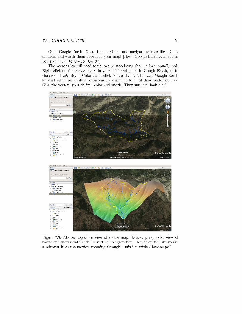
Open Google Earth. Go to File → Open, and navigate to your �les. Clickon them and watch them appear in your map! [Hey - Google Earth even zoomsyou straight in to Gordon Gulch!]

The vector �les will need some love to stop being that uniform spindly red.Right-click on the vector layers in your left-hand panel in Google Earth, go tothe second tab [Style, Color], and click �share style�. This way Google Earthknows that it can apply a consistent color scheme to all of these vector objects.Give the vectors your desired color and width. They sure can look nice!

Figure 7.3: Above: top-down view of vector map. Below: perspective view ofraster and vector data with 3× vertical exaggeration. Don't you feel like you'rea scientist from the movies, zooming through a mission-critical landscape?

60 CHAPTER 7. FILE INPUT AND OUTPUT

Chapter 8

Writing and Executing

Scripts

8.1 Text editors for programming

You will want a good basic text editor for programming. These will highlightand color the portions of the code according to their purpose, and (especially ifyou haven't programmed before) will make understanding what you are doingmuch more intuitive. The text editors I have used (or heard good things about)are:

� Windows: notepad++

� Mac: TextWrangler and gedit

� Linux: gedit (comes pre-installed)

8.2 Shell scripting (Bash)

Bash is an old language that is very nice for creating quick-and-dirty scripts toautomate tasks. This section provides an introduction to Bash, some informa-tion on regular expressions, and how information can be piped to and from �lesto make the scripts run.

for file in *.txt

do

echo $file

done

# Create an empty file calld "fnames.txt": this is what the ">"

# without any content on the left side of the ">" does

> fnames.txt

for file in *.txt

61

62 CHAPTER 8. WRITING AND EXECUTING SCRIPTS

do

# Append new lines with all of the file names you find

# ">>" means append to file; ">" means create file

# Here, you are "piping" the output of "echo" into

# the file fnames.txt, instead of having it appear

# in the standard output (i.e. the terminal window)

echo $file >> fnames.txt

done

Inside a GRASS environment, we can use GRASS commands here. Let'sstart by exporting a list of the raster �les that we have:

# Get a full list of GRASS raster files, and pipe it to "rasters.txt"

g.list rast > rasters.txt

Use the vi (or your preferred) text editor to look at the �le.

vi rasters.txt

As you can see, it isn't formatted in a nice way, with each entry on its own line.(Press �:q�, then �ENTER� to exit when you are done viewing.) This calls fora tool called sed, which can parse regular expressions. We will do a lot of �ndand replace commands with sed.

First, let's remove the �rst, second and last lines:

cp rasters.txt rasters.txt.backup # backup copy is good!

sed -i '1 d' rasters.txt # Replace first line with nothing

sed -i '1 d' rasters.txt # Replace second line with nothing (it is now the 1st

line!)

sed -i '$ d' rasters.txt # Replace last line with nothing

Now, let's replace the spaces (any number of them) with newline characters,and then remove blank lines that would be read as supposed raster names.

sed -i 's/ \+/\n/g' rasters.txt # Turns the spaces into newlines, and your data

into a single column!

sed -i '/^$/d' rasters.txt # Removes blank lines

Use vi or another text editor to admire your handiwork!

Now, let's display all of these in order... wait, maybe that isn't a good idea...if you get bored of the display of all of your raster maps, press CTRL+C tostop the process.

d.mon x0 # start a display monitor

# Then get the values of the lines

while read line

do

echo $line # print raster name to screen

d.rast $line # display that raster!

sleep 2 # wait two seconds

d.erase # Erase the monitor

done < rasters.txt # Pipe in the text file for reading

8.3. PYTHON SCRIPTING 63

8.3 Python scripting

This section won't be written for some time, but this is how I write most of mylarge GRASS programs. It allows much easier handling of variables, especiallyin lists and arrays, than Bash scripting. It also has some nice plotting utili-ties which can produce really pretty �gures (Matplotlib's basemap, made by ascientist at NOAA here in Boulder).

Information on Python scripting can be found on the GRASS wiki at:

� http://grass.osgeo.org/wiki/GRASS_and_Python

� http://grass.osgeo.org/wiki/GRASS_Python_Scripting_Library

� http://grass.osgeo.org/wiki/Converting_Bash_scripts_to_Python

These sources are fairly comprehensive and link to additional sources of infor-mation. This is a major reason why I am in no hurry to write this section:good information exists, and once you know GRASS and Python, all you needto know are the Python modules to import and the syntax to access GRASSfunctionality. These Wiki articles comprise most (almost all?) of what I know(and some more besides: I hadn't seen some of these articles before writing thisparagraph, and some have seen signi�cant overhaul in recent weeks/months),and link to the rest of what I use.

The Wiki documentation is skimpy on vector handling (Python is still fairlynew to GRASS), but the Python API is largely built, so I have used infor-mation from the GRASS programmer's manual (a useful resource in general)to work through these issues. See http://grass.osgeo.org/programming6/

namespacepython_1_1vector.html for the GRASS 6.5 version. I still haven'tfound a way to write data to GRASS vectors from Python data structures: Ican use Python to run the standard GRASS vector commands, though.

The full GRASS Progammer's Manual (6.5, but similar to 6.4, and easilyfound via a web search) is http://grass.osgeo.org/programming6/pythonlib.html (here open to the Python section, but with access to the whole thing vis-ible).

Python scripting has also provided me with a way to run my numericalmodels in a geospatially-registered environment. This is great, because it meansthat my model results can be compared instantly with real-world data. To get ataste of both GRASS Python scripting and model integration, check out a copyof my �exural isostasy model from the CSDMS subversion repository:

svn co https://csdms.colorado.edu/svn/flexure

Go to flexure/trunk and look at r.flexure.py. It's still a little rough asof when I'm writing this manual (16 April 2012), but hey � it works � and itcan be a sign of greater things to come!

64 CHAPTER 8. WRITING AND EXECUTING SCRIPTS

Chapter 9

Wrap-up

9.1 Thoughts from the Author

I hope that this manual has been useful to you. Please let me know if there isanything that needs to be �xed, if you'd want to help and/or expand it in anyway, or if you have other questions or suggestions. I really hope that this helpsyou to be more e�cient at the computer, be able to do more insightful analysesin a shorter period of time, and avoid paying sky-high fees for Arc and burstinginto tears as it crashes and burns and takes your day of work with it.

The open-source community in Earth-surface processes is growing, as exem-pli�ed by projects like the Community Surface Dynamics Modeling System (CS-DMS). As geomorphologists, sedimentologists, land-use dynamicists, and otherEarth-surface scientists, we are increasingly able to model complex natural sys-tems, and our capacity for �eld data collection continues to grow. Combiningour work into a GIS�especially an open-source GIS like GRASS that has itsown community with goals that are not so di�erent from those that many Earth-surface scientists have�is a way I see into the future of data�model integrationthat will allow us to better predict future events and expain the Earth's past.

This manual has been an entirely free-time project to introduce the geomor-phic community to an open-source, highly-automatable GIS and some of theneat things you can do with it. As such, I won't always be able to answer allquestions in a timely manner, but I really, really promise that I will try.

Happy geospatial adventures to all of you!

�Andy, 16 April 2012

65

66 CHAPTER 9. WRAP-UP

9.2 Useful Resources

For more information and/or further exploration of open source GIS, check outthe following (some of which I have mentioned in the text):

� Markus Neteler and Helena Mitasova, 2008, Open Source GIS: A GRASS

GIS Approach. Third Edition. http://www.grassbook.org/

� the GRASS GIS Wiki, http://grass.osgeo.org/wiki/GRASS-Wiki

� The Open Source Geospatial Foundation, http://www.osgeo.org/, whereyou can download the software, learn about it, and

� the main GRASS GIS website, http://grass.osgeo.org/

� Quantum GIS, a nice open-source point-and-click GIS that can plug in toGRASS as an attractive front-end: http://www.qgis.org/

9.3 Future Plans

This section is mostly for the author, but it is written in the text so readers canhave an idea of what to (maybe) expect:

1. Compilation instructions, �les with c�ags, etc.

2. Geomorphic Python examples and some general Python background

3. Code from speci�c projects and/or codes that I have written to do generally-useful tasks (e.g., regional-scale stream pro�les, terrace identi�cation)

4. CSDMS and GRASS � but I need to work with CSDMS �rst to see if I cancreate a generic GRASS wrapper for their interfaces, and I would need tohave time to do that...

5. Write a LaTeX environment to make boldface monospaced font typesetinstead of co-opting the URL

6. Add a section on interpolating data going from point clouds to grids, andLiDAR processing

7. Remote sensing: learn it, or talk to someone who knows it, and then writeabout it

9.4. CONTACT INFORMATION 67

9.4 Contact Information

Andy WickertUniversity of Colorado

Department of Geological Sciences andInstitute of Arctic and Alpine Research

Street / package address 1560 30th StreetBoulder, CO 80303

Mailing (non-packages) address Campus Box 450Boulder, CO 80309-0450

E-mail: wickert@colorado.eduPermanent forwarding email: awickert@alum.mit.edu(because I'm graduating from CU soon-ish... right, Bob?)