Embed Size (px)
Citation preview
Graph Visualization:
Topology-Shape-Metrics
Topology-Shape-Metrics
1. Background
• Planarity
• Topology
2. The topology-shape-metrics approach
1. Topology
2. Shape
3. Metrics
3. Remarks

Background: Planarity
7
5
1
9
6
2
3
4
0
8
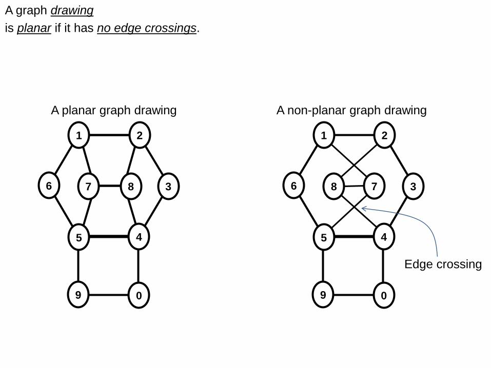
A graph drawing
is planar if it has no edge crossings.
7
5
1
9
6
2
3
4
0
8
A planar graph drawing A non-planar graph drawing
Edge crossing
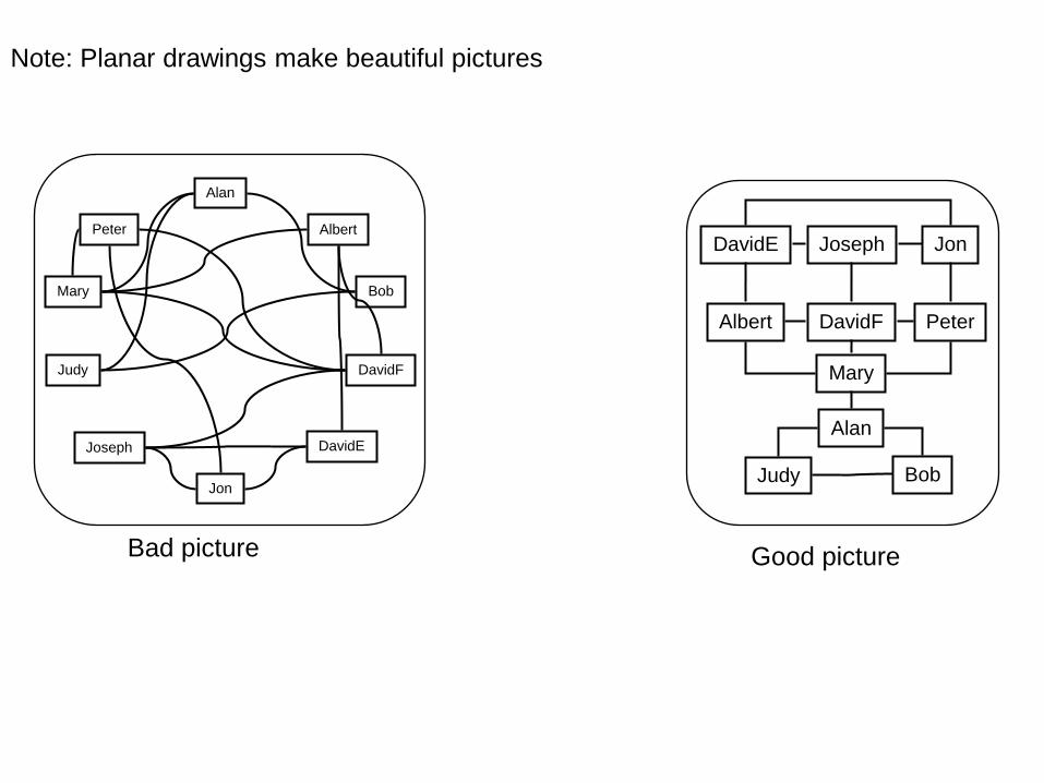
Note: Planar drawings make beautiful pictures
Mary Bob
Peter
Jon
DavidF
Alan
Joseph
Judy
Albert
DavidE
Peter
Mary
Jon
DavidF
Alan
Joseph
Bob Judy
Albert
DavidE
Bad picture Good picture
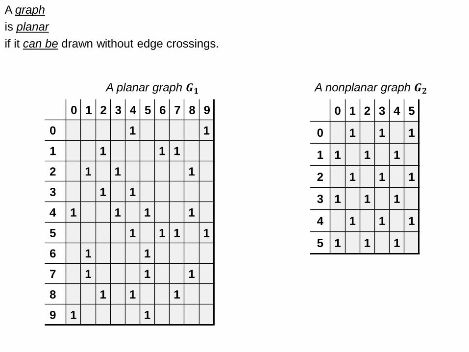
A graph
is planar
if it can be drawn without edge crossings.
0 1 2 3 4 5 6 7 8 9
0 1 1
1 1 1 1
2 1 1 1
3 1 1
4 1 1 1 1
5 1 1 1 1
6 1 1
7 1 1 1
8 1 1 1
9 1 1
A planar graph 𝑮𝟏
0 1 2 3 4 5
0 1 1 1
1 1 1 1
2 1 1 1
3 1 1 1
4 1 1 1
5 1 1 1
A nonplanar graph 𝑮𝟐
7
5
1
9
6
2
3
4
0
8
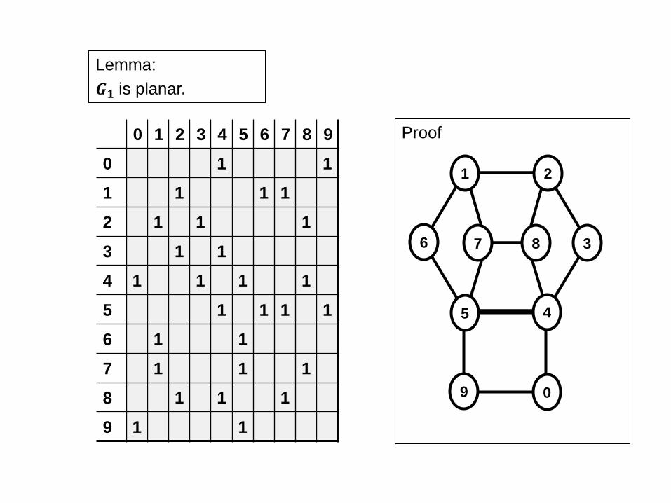
Lemma:
𝑮𝟏 is planar.
0 1 2 3 4 5 6 7 8 9
0 1 1
1 1 1 1
2 1 1 1
3 1 1
4 1 1 1 1
5 1 1 1 1
6 1 1
7 1 1 1
8 1 1 1
9 1 1
Proof
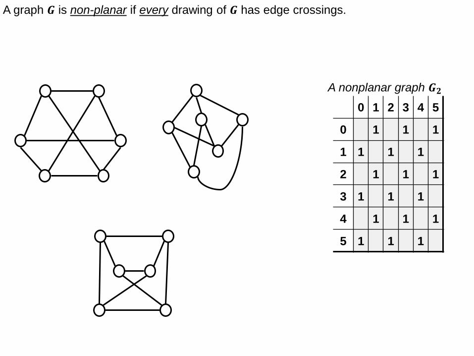
A graph 𝑮 is non-planar if every drawing of 𝑮 has edge crossings.
0 1 2 3 4 5
0 1 1 1
1 1 1 1
2 1 1 1
3 1 1 1
4 1 1 1
5 1 1 1
A nonplanar graph 𝑮𝟐
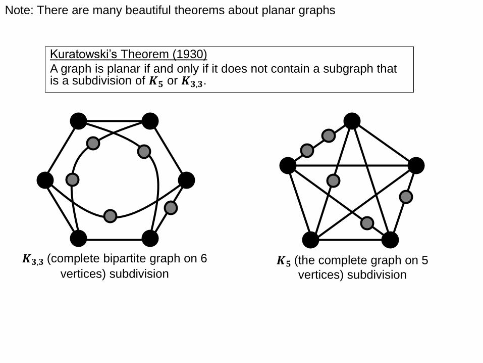
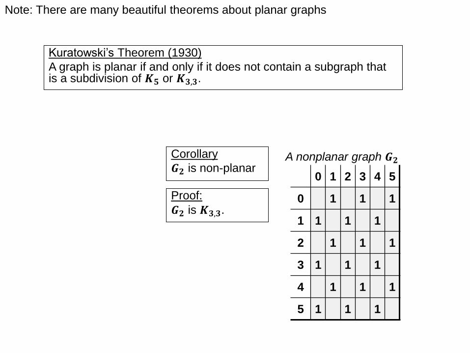
Kuratowski’s Theorem (1930)
A graph is planar if and only if it does not contain a subgraph that is a subdivision of 𝑲𝟓 or 𝑲𝟑,𝟑.
𝑲𝟓 (the complete graph on 5
vertices) subdivision
𝑲𝟑,𝟑 (complete bipartite graph on 6
vertices) subdivision
Note: There are many beautiful theorems about planar graphs
Kuratowski’s Theorem (1930)
A graph is planar if and only if it does not contain a subgraph that is a subdivision of 𝑲𝟓 or 𝑲𝟑,𝟑.
Note: There are many beautiful theorems about planar graphs
Corollary
𝑮𝟐 is non-planar 0 1 2 3 4 5
0 1 1 1
1 1 1 1
2 1 1 1
3 1 1 1
4 1 1 1
5 1 1 1
A nonplanar graph 𝑮𝟐
Proof:
𝑮𝟐 is 𝑲𝟑,𝟑.
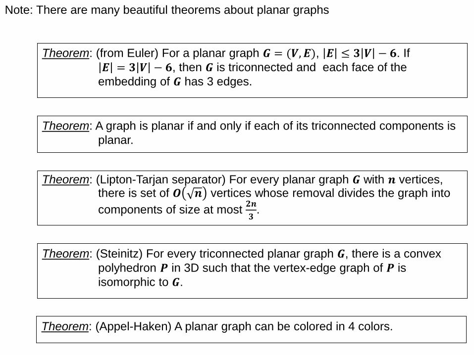
Theorem: A graph is planar if and only if each of its triconnected components is
planar.
Note: There are many beautiful theorems about planar graphs
Theorem: (Appel-Haken) A planar graph can be colored in 4 colors.
Theorem: (from Euler) For a planar graph 𝑮 = (𝑽, 𝑬), 𝑬 ≤ 𝟑 𝑽 − 𝟔. If 𝑬 = 𝟑 𝑽 − 𝟔, then 𝑮 is triconnected and each face of the
embedding of 𝑮 has 3 edges.
Theorem: (Steinitz) For every triconnected planar graph 𝑮, there is a convex
polyhedron 𝑷 in 3D such that the vertex-edge graph of 𝑷 is
isomorphic to 𝑮.
Theorem: (Lipton-Tarjan separator) For every planar graph 𝑮 with 𝒏 vertices, there is set of 𝑶 𝒏 vertices whose removal divides the graph into
components of size at most 𝟐𝒏
𝟑.
Remarks: Planar graphs and real-world graphs
Most real-world graphs are not planar
But most are “nearly” planar in that deletion of 𝒐(𝒏) edges gives a planar graph
• scale-free networks are locally dense and globally sparse
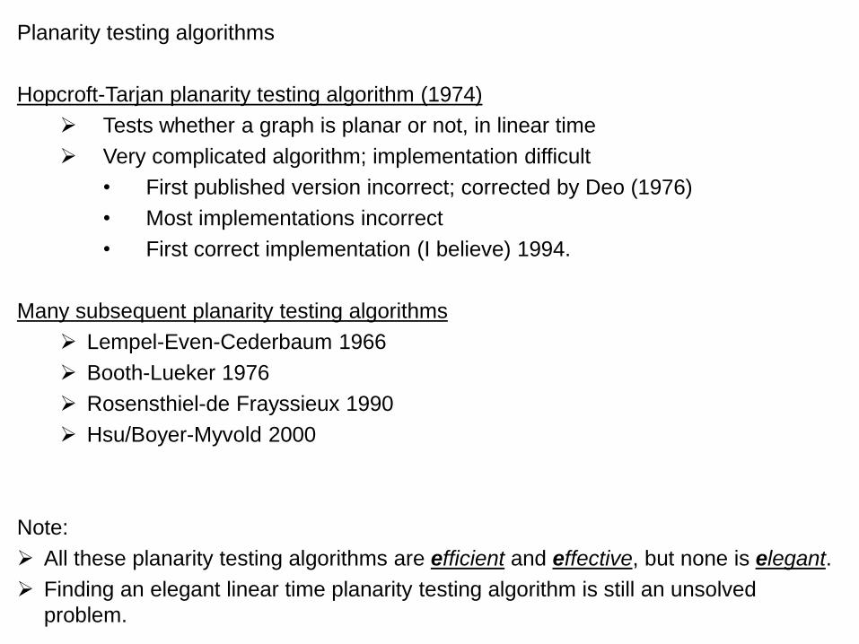
Planarity testing algorithms
Hopcroft-Tarjan planarity testing algorithm (1974)
Tests whether a graph is planar or not, in linear time
Very complicated algorithm; implementation difficult
• First published version incorrect; corrected by Deo (1976)
• Most implementations incorrect
• First correct implementation (I believe) 1994.
Many subsequent planarity testing algorithms
Lempel-Even-Cederbaum 1966
Booth-Lueker 1976
Rosensthiel-de Frayssieux 1990
Hsu/Boyer-Myvold 2000
Note:
All these planarity testing algorithms are efficient and effective, but none is elegant.
Finding an elegant linear time planarity testing algorithm is still an unsolved
problem.

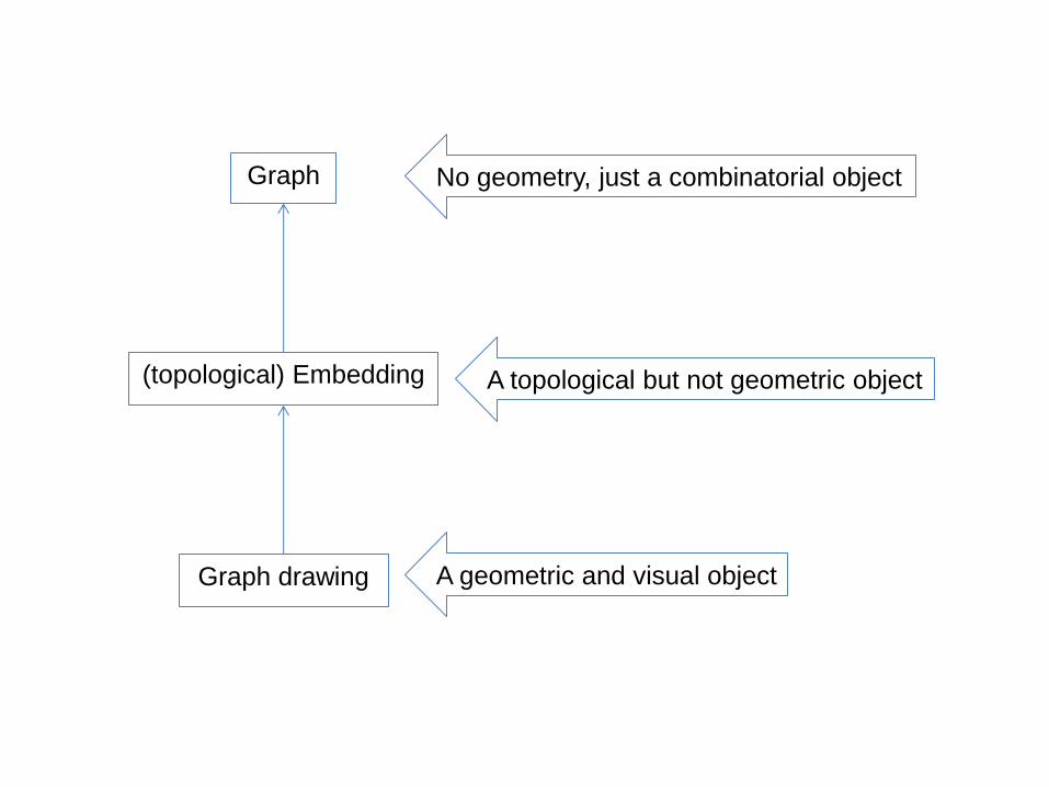
Background: Topology
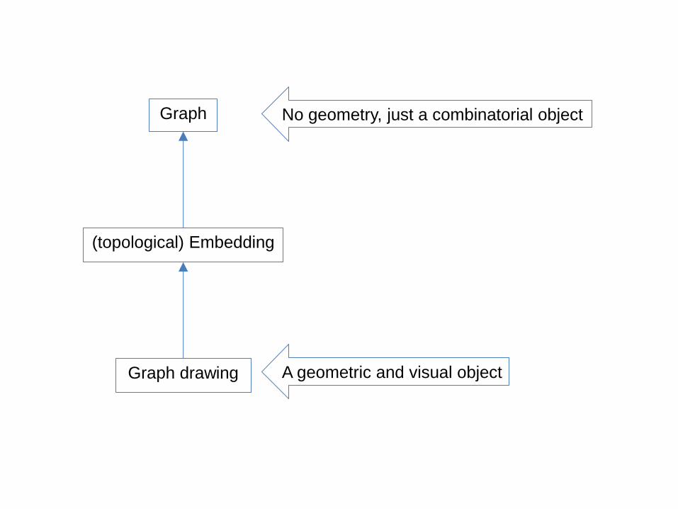
Graph
(topological) Embedding
Graph drawing
No geometry, just a combinatorial object
A geometric and visual object
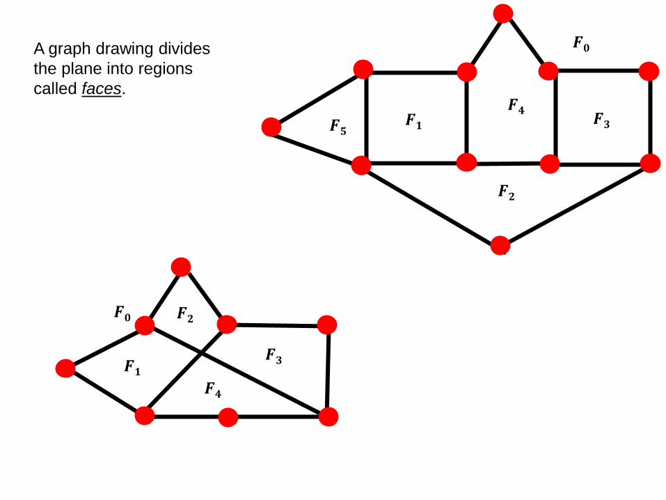
A graph drawing divides
the plane into regions
called faces.
𝑭𝟏
𝑭𝟎 𝑭𝟐
𝑭𝟒
𝑭𝟑
𝑭𝟏
𝑭𝟎
𝑭𝟐
𝑭𝟑 𝑭𝟒
𝑭𝟓
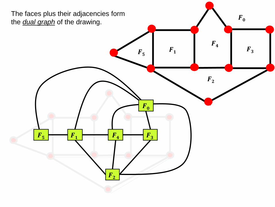
The faces plus their adjacencies form
the dual graph of the drawing.
𝑭𝟏
𝑭𝟎
𝑭𝟐
𝑭𝟑 𝑭𝟒
𝑭𝟓
𝑭𝟑 𝑭𝟏
𝑭𝟎
𝑭𝟒 𝑭𝟓
𝑭𝟐
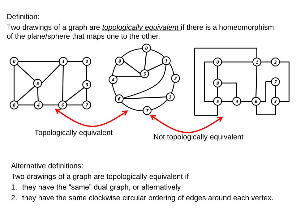
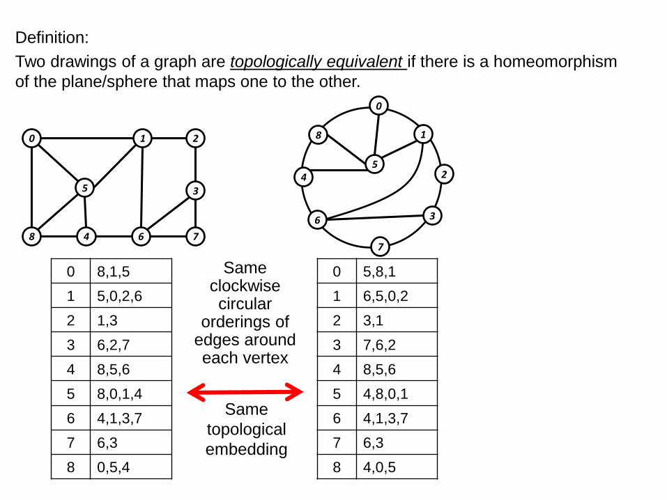
Definition:
Two drawings of a graph are topologically equivalent if there is a homeomorphism
of the plane/sphere that maps one to the other.
1
3 5
8 4 6
2 0
7
1
3
5
8
4
6
2
0
7
1
3 5
8
4 6
2 0
7
Alternative definitions:
Two drawings of a graph are topologically equivalent if
1. they have the “same” dual graph, or alternatively
2. they have the same clockwise circular ordering of edges around each vertex.
Topologically equivalent Not topologically equivalent
1
3 5
8 4 6
2 0
7
1
3
5
8
4
6
2
0
7
0 8,1,5
1 5,0,2,6
2 1,3
3 6,2,7
4 8,5,6
5 8,0,1,4
6 4,1,3,7
7 6,3
8 0,5,4
0 5,8,1
1 6,5,0,2
2 3,1
3 7,6,2
4 8,5,6
5 4,8,0,1
6 4,1,3,7
7 6,3
8 4,0,5
Same
topological
embedding
Same clockwise circular
orderings of edges around each vertex
Definition:
Two drawings of a graph are topologically equivalent if there is a homeomorphism
of the plane/sphere that maps one to the other.
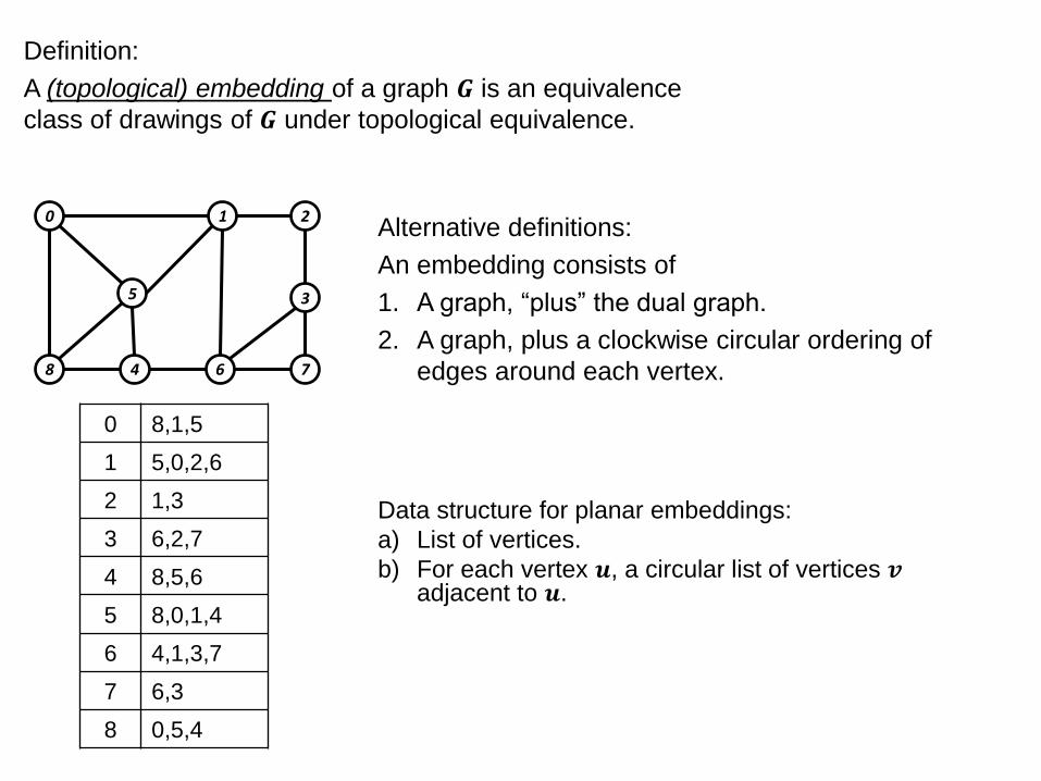
Definition:
A (topological) embedding of a graph 𝑮 is an equivalence
class of drawings of 𝑮 under topological equivalence.
Data structure for planar embeddings:
a) List of vertices.
b) For each vertex 𝒖, a circular list of vertices 𝒗 adjacent to 𝒖.
1
3 5
8 4 6
2 0
7
0 8,1,5
1 5,0,2,6
2 1,3
3 6,2,7
4 8,5,6
5 8,0,1,4
6 4,1,3,7
7 6,3
8 0,5,4
Alternative definitions:
An embedding consists of
1. A graph, “plus” the dual graph.
2. A graph, plus a clockwise circular ordering of
edges around each vertex.
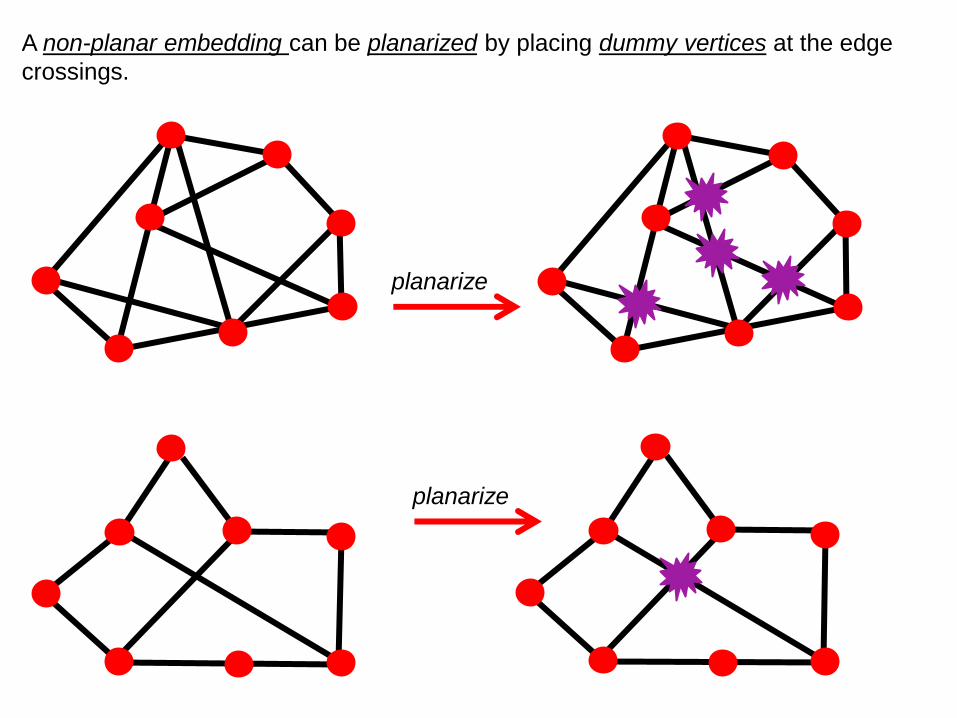
A non-planar embedding can be planarized by placing dummy vertices at the edge
crossings.
planarize
planarize
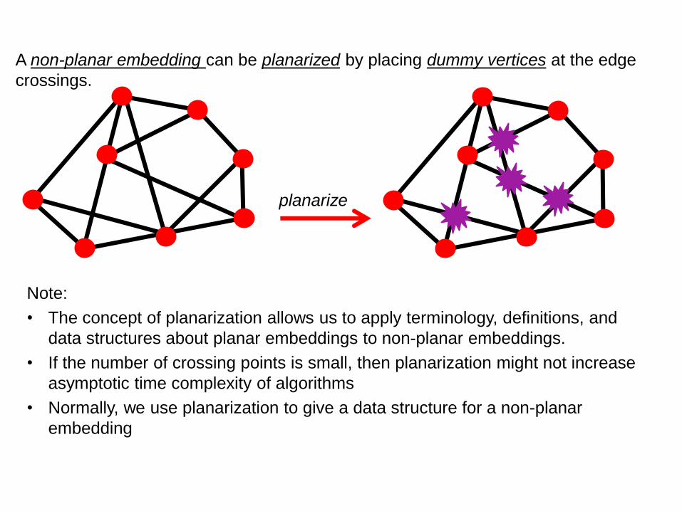
A non-planar embedding can be planarized by placing dummy vertices at the edge
crossings.
planarize
Note:
• The concept of planarization allows us to apply terminology, definitions, and
data structures about planar embeddings to non-planar embeddings.
• If the number of crossing points is small, then planarization might not increase
asymptotic time complexity of algorithms
• Normally, we use planarization to give a data structure for a non-planar
embedding
Planar embedding algorithms
Most planarity testing algorithms “can be adjusted” to output a planar
embedding of a planar graph in linear time.
All these algorithms are efficient and effective; none is elegant.

3. Graph drawings
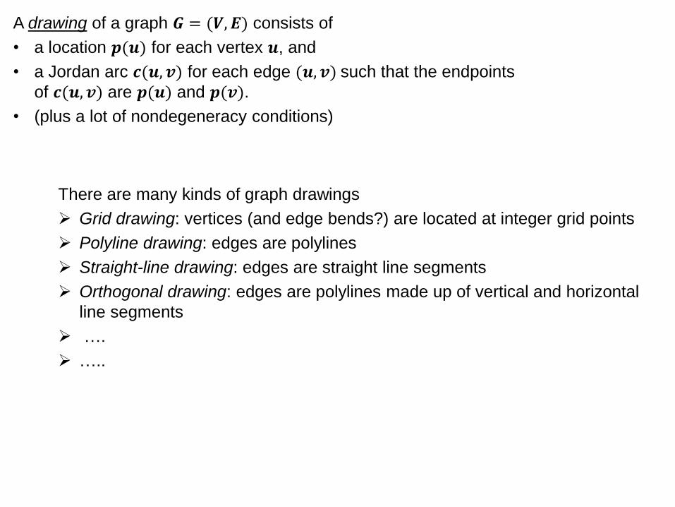
A drawing of a graph 𝑮 = (𝑽, 𝑬) consists of
• a location 𝒑(𝒖) for each vertex 𝒖, and
• a Jordan arc 𝒄(𝒖, 𝒗) for each edge (𝒖, 𝒗) such that the endpoints
of 𝒄(𝒖, 𝒗) are 𝒑(𝒖) and 𝒑(𝒗).
• (plus a lot of nondegeneracy conditions)
There are many kinds of graph drawings
Grid drawing: vertices (and edge bends?) are located at integer grid points
Polyline drawing: edges are polylines
Straight-line drawing: edges are straight line segments
Orthogonal drawing: edges are polylines made up of vertical and horizontal
line segments
….
…..
5
2 0 1
8
3 7 4 6
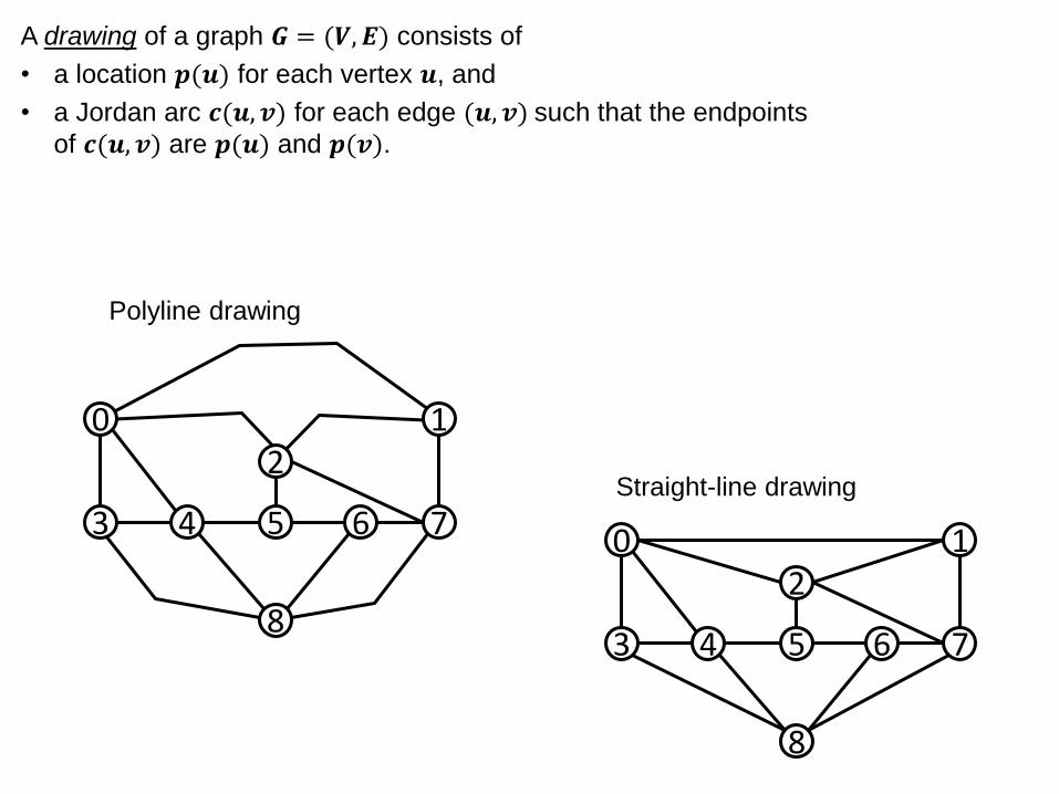
Straight-line drawing
5
2 0 1
8
3 7 4 6
Polyline drawing
A drawing of a graph 𝑮 = (𝑽, 𝑬) consists of
• a location 𝒑(𝒖) for each vertex 𝒖, and
• a Jordan arc 𝒄(𝒖, 𝒗) for each edge (𝒖, 𝒗) such that the endpoints
of 𝒄(𝒖, 𝒗) are 𝒑(𝒖) and 𝒑(𝒗).
5
2 0
1
8
3
7
4
6
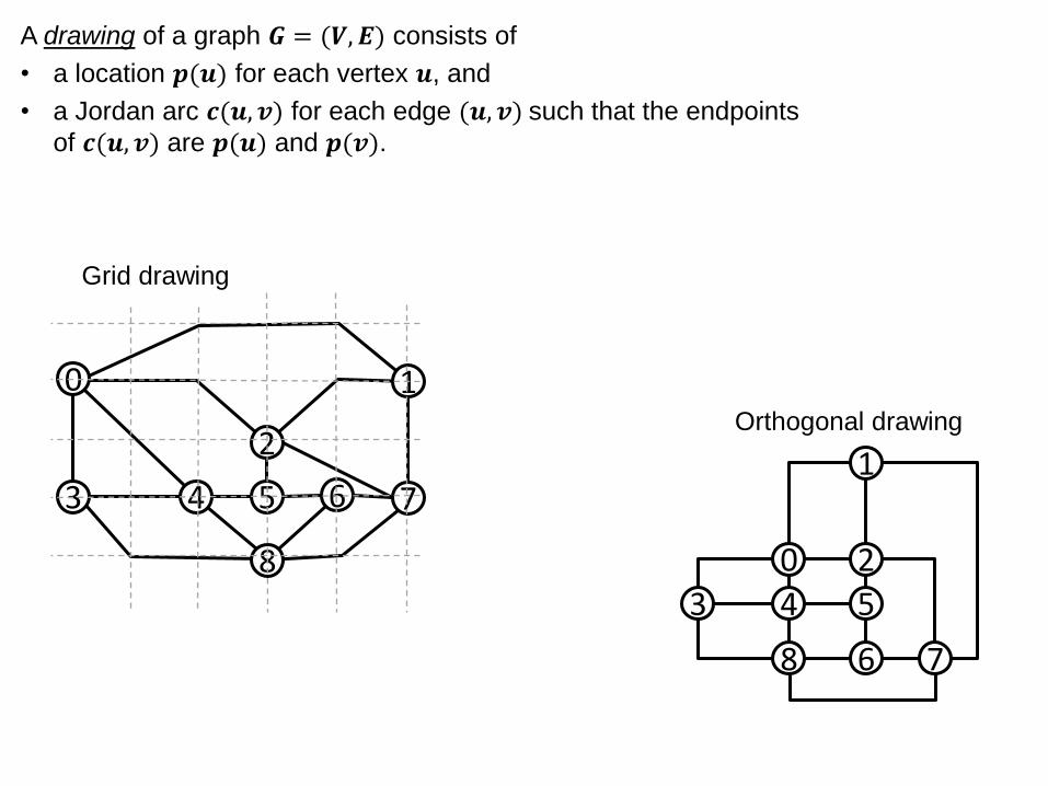
Orthogonal drawing
5
2
0 1
8
3 7 4 6
Grid drawing
A drawing of a graph 𝑮 = (𝑽, 𝑬) consists of
• a location 𝒑(𝒖) for each vertex 𝒖, and
• a Jordan arc 𝒄(𝒖, 𝒗) for each edge (𝒖, 𝒗) such that the endpoints
of 𝒄(𝒖, 𝒗) are 𝒑(𝒖) and 𝒑(𝒗).

5
2
1
8
3
7
4
6
0
Orthogonal grid drawing
A drawing of a graph 𝑮 = (𝑽, 𝑬) consists of
• a location 𝒑(𝒖) for each vertex 𝒖, and
• a Jordan arc 𝒄(𝒖, 𝒗) for each edge (𝒖, 𝒗) such that the endpoints
of 𝒄(𝒖, 𝒗) are 𝒑(𝒖) and 𝒑(𝒗).
Graph
(topological) Embedding
Graph drawing
No geometry, just a combinatorial object
A geometric and visual object
A topological but not geometric object
Topology-shape-metrics approach
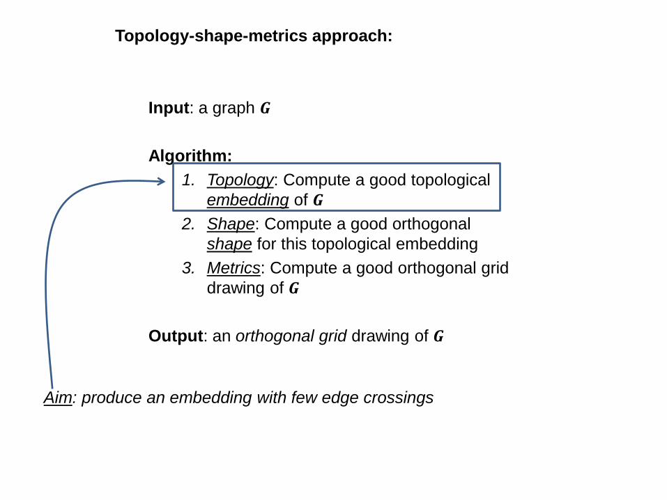
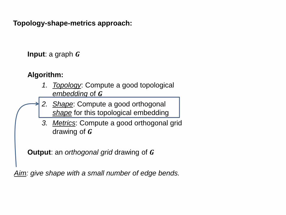
Topology-shape-metrics approach:
Input: a graph 𝑮
Algorithm:
1. Topology: Compute a good topological
embedding of 𝑮
2. Shape: Compute a good orthogonal
shape for this topological embedding
3. Metrics: Compute a good orthogonal grid
drawing of 𝑮
Output: an orthogonal grid drawing of 𝑮
Aim: produce an embedding with few edge crossings
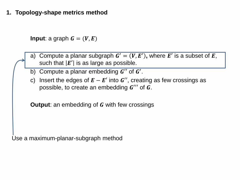
1. Topology-shape metrics method
Input: a graph 𝑮 = (𝑽, 𝑬)
a) Compute a planar subgraph 𝑮′ = 𝑽, 𝑬′ , where 𝑬′ is a subset of 𝑬, such that 𝑬′ is as large as possible.
b) Compute a planar embedding 𝑮′′ of 𝑮′.
c) Insert the edges of 𝑬 − 𝑬′ into 𝑮′′, creating as few crossings as
possible, to create an embedding 𝑮′′′ of 𝑮.
Output: an embedding of 𝑮 with few crossings
Use a maximum-planar-subgraph method
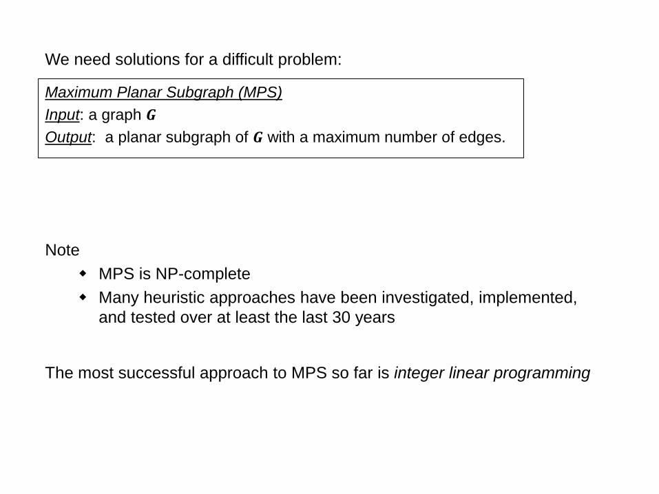
We need solutions for a difficult problem:
The most successful approach to MPS so far is integer linear programming
Note
MPS is NP-complete
Many heuristic approaches have been investigated, implemented,
and tested over at least the last 30 years
Maximum Planar Subgraph (MPS)
Input: a graph 𝑮
Output: a planar subgraph of 𝑮 with a maximum number of edges.
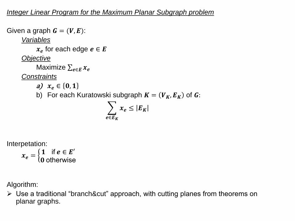
Integer Linear Program for the Maximum Planar Subgraph problem
Given a graph 𝑮 = (𝑽, 𝑬):
Variables
𝒙𝒆 for each edge 𝒆 ∈ 𝑬
Objective
Maximize 𝒙𝒆𝒆∈𝑬
Constraints
a) 𝒙𝒆 ∈ 𝟎, 𝟏
b) For each Kuratowski subgraph 𝑲 = 𝑽𝑲, 𝑬𝑲 of 𝑮:
𝒙𝒆𝒆∈𝑬𝑲
≤ 𝑬𝑲
Interpetation:
𝒙𝒆 = 𝟏 if 𝒆 ∈ 𝑬′𝟎 otherwise
Algorithm:
Use a traditional “branch&cut” approach, with cutting planes from theorems on planar graphs.
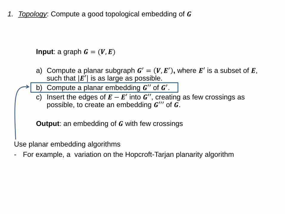
1. Topology: Compute a good topological embedding of 𝑮
Input: a graph 𝑮 = (𝑽, 𝑬)
a) Compute a planar subgraph 𝑮′ = 𝑽, 𝑬′ , where 𝑬′ is a subset of 𝑬, such that 𝑬′ is as large as possible.
b) Compute a planar embedding 𝑮′′ of 𝑮′.
c) Insert the edges of 𝑬 − 𝑬′ into 𝑮′′, creating as few crossings as possible, to create an embedding 𝑮′′′ of 𝑮.
Output: an embedding of 𝑮 with few crossings
Use planar embedding algorithms
- For example, a variation on the Hopcroft-Tarjan planarity algorithm
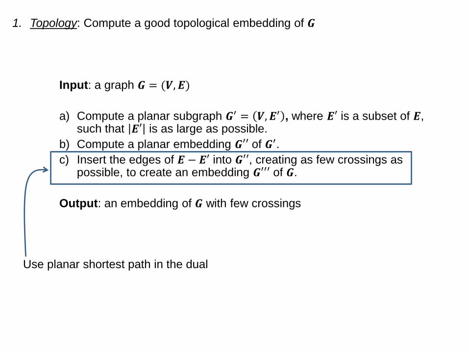
1. Topology: Compute a good topological embedding of 𝑮
Input: a graph 𝑮 = (𝑽, 𝑬)
a) Compute a planar subgraph 𝑮′ = 𝑽, 𝑬′ , where 𝑬′ is a subset of 𝑬, such that 𝑬′ is as large as possible.
b) Compute a planar embedding 𝑮′′ of 𝑮′.
c) Insert the edges of 𝑬 − 𝑬′ into 𝑮′′, creating as few crossings as possible, to create an embedding 𝑮′′′ of 𝑮.
Output: an embedding of 𝑮 with few crossings
Use planar shortest path in the dual
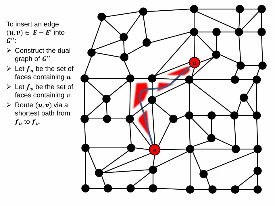
To insert an edge
(𝒖, 𝒗) ∈ 𝑬 − 𝑬′ into
𝑮′′:
Construct the dual
graph of 𝑮′′
Let 𝒇𝒖 be the set of
faces containing 𝒖
Let 𝒇𝒗 be the set of
faces containing 𝒗
Route (𝒖, 𝒗) via a
shortest path from
𝒇𝒖 to 𝒇𝒗.
1
3 5
8 4 6
2 0
7
1
3 5
8 4 6
0
7
1
3
5
8 4 6
2 0
7
1
3 5
8 4 6
2 0
7
1
5
8 4 6
2 0
7
1 2
1
5
8 4
6
0
v
u
Topology-shape-metrics approach:
Input: a graph 𝑮
Algorithm:
1. Topology: Compute a good topological
embedding of 𝑮
2. Shape: Compute a good orthogonal
shape for this topological embedding
3. Metrics: Compute a good orthogonal grid
drawing of 𝑮
Output: an orthogonal grid drawing of 𝑮
Aim: give shape with a small number of edge bends.
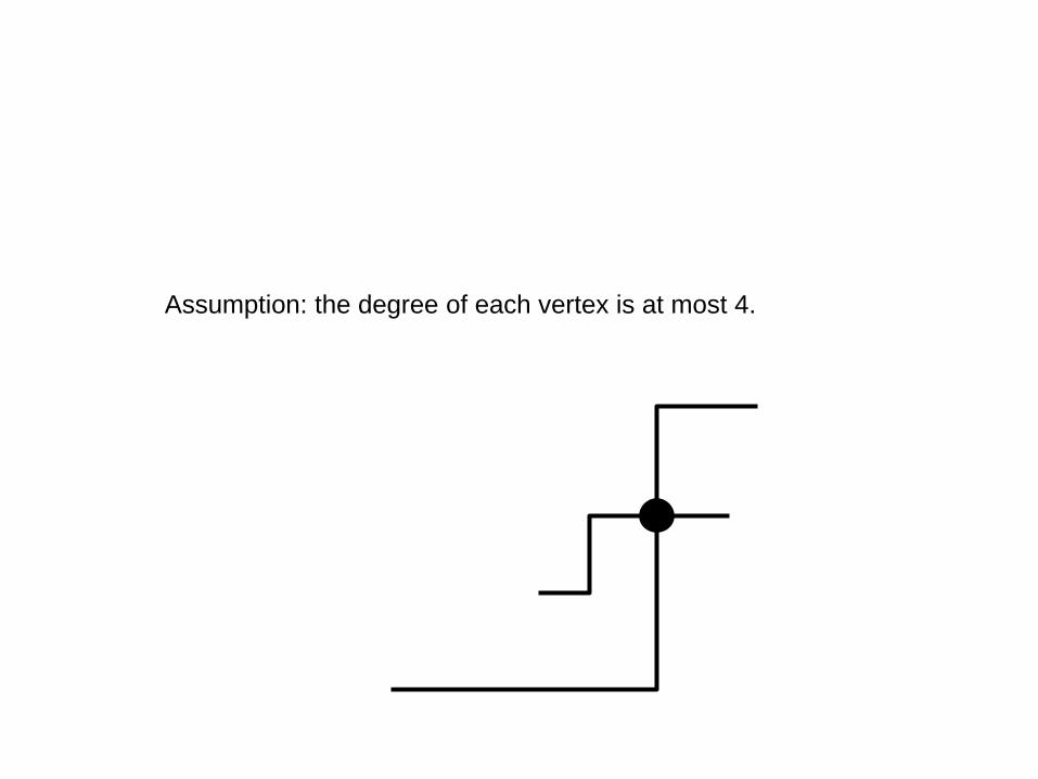
Assumption: the degree of each vertex is at most 4.
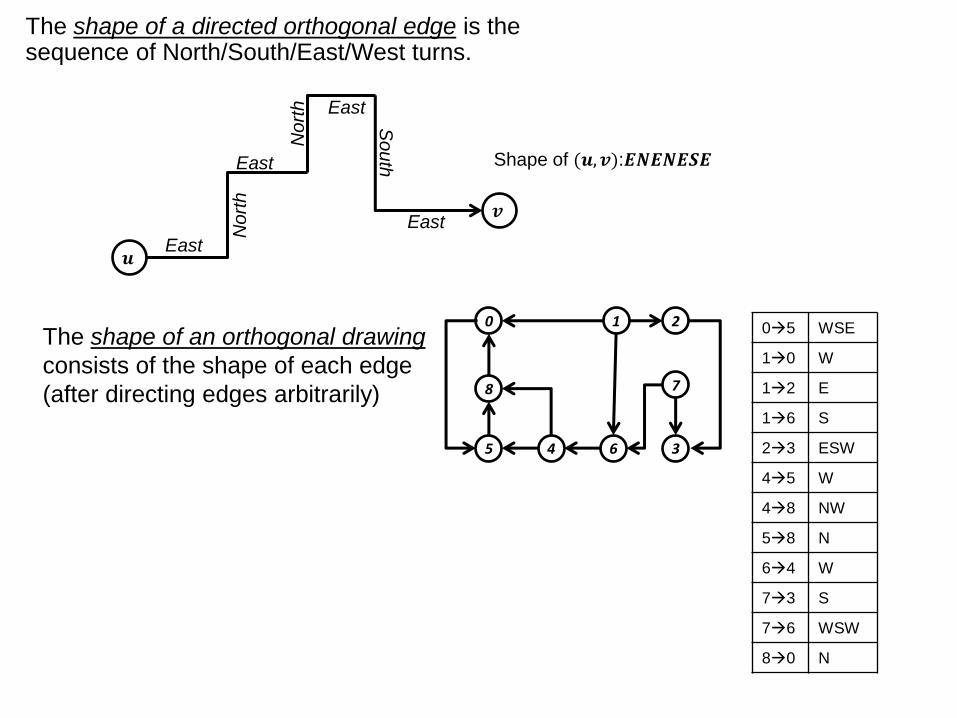
The shape of a directed orthogonal edge is the sequence of North/South/East/West turns.
𝒖
𝒗
Shape of (𝒖, 𝒗):𝑬𝑵𝑬𝑵𝑬𝑺𝑬
East
East
East
East N
ort
h
No
rth
So
uth
The shape of an orthogonal drawing
consists of the shape of each edge
(after directing edges arbitrarily)
1
3 5
8
4 6
2 0
7
05 WSE
10 W
12 E
16 S
23 ESW
45 W
48 NW
58 N
64 W
73 S
76 WSW
80 N
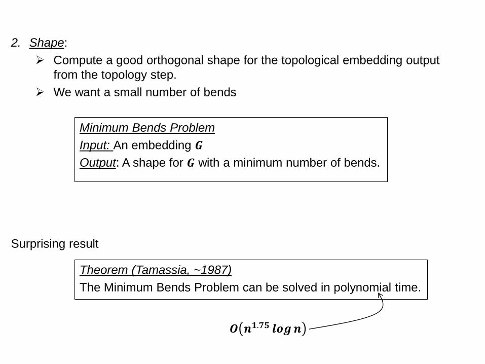
2. Shape:
Compute a good orthogonal shape for the topological embedding output
from the topology step.
We want a small number of bends
Minimum Bends Problem
Input: An embedding 𝑮
Output: A shape for 𝑮 with a minimum number of bends.
Surprising result
Theorem (Tamassia, ~1987)
The Minimum Bends Problem can be solved in polynomial time.
𝑶 𝒏𝟏.𝟕𝟓 𝒍𝒐𝒈𝒏
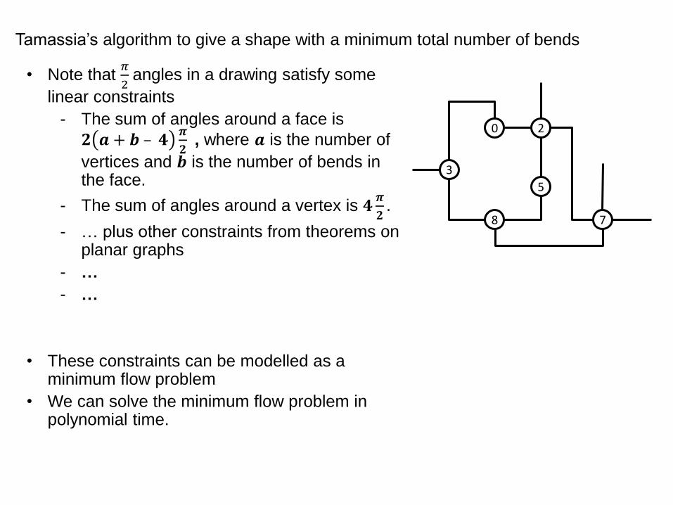
Tamassia’s algorithm to give a shape with a minimum total number of bends
5
2 0
8
3
7
• Note that 𝜋
2 angles in a drawing satisfy some
linear constraints
- The sum of angles around a face is
𝟐 𝒂 + 𝒃 – 𝟒𝝅
𝟐 , where 𝒂 is the number of
vertices and 𝒃 is the number of bends in the face.
- The sum of angles around a vertex is 𝟒𝝅
𝟐.
- … plus other constraints from theorems on planar graphs
- …
- …
• These constraints can be modelled as a minimum flow problem
• We can solve the minimum flow problem in polynomial time.
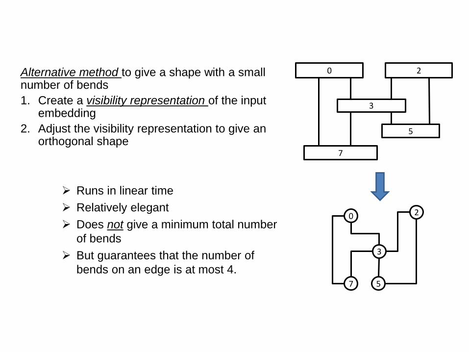
Alternative method to give a shape with a small number of bends
1. Create a visibility representation of the input embedding
2. Adjust the visibility representation to give an orthogonal shape
Runs in linear time
Relatively elegant
Does not give a minimum total number
of bends
But guarantees that the number of
bends on an edge is at most 4. 5
2 0
3
7
5
2 0
3
7
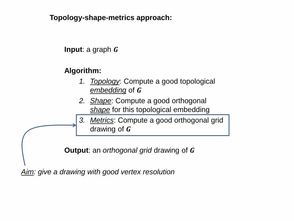
Topology-shape-metrics approach:
Input: a graph 𝑮
Algorithm:
1. Topology: Compute a good topological
embedding of 𝑮
2. Shape: Compute a good orthogonal
shape for this topological embedding
3. Metrics: Compute a good orthogonal grid
drawing of 𝑮
Output: an orthogonal grid drawing of 𝑮
Aim: give a drawing with good vertex resolution
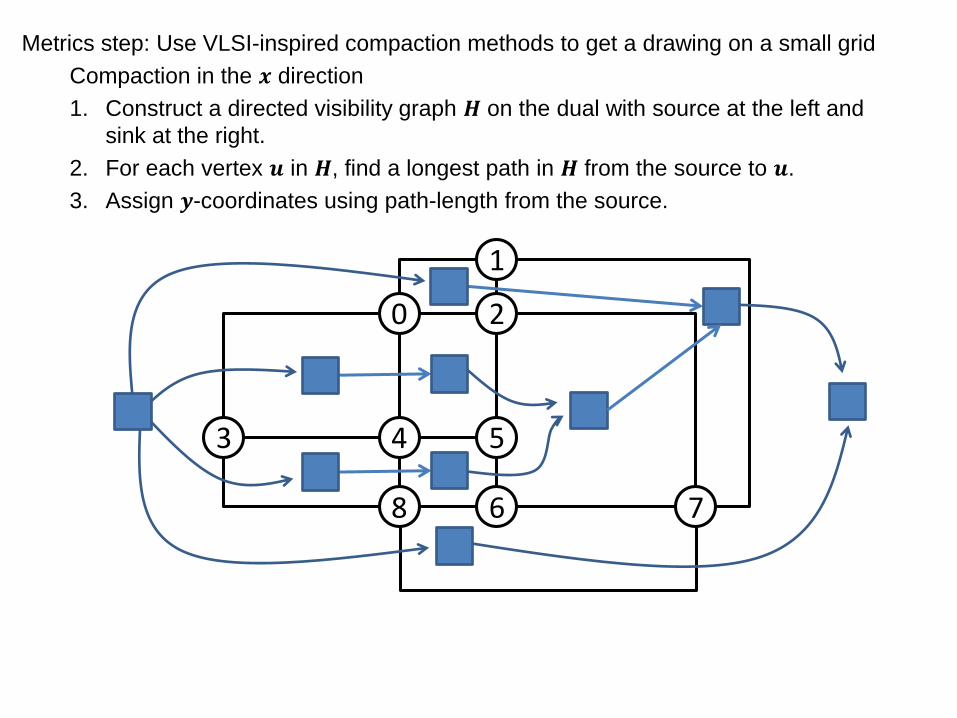
Metrics step: Use VLSI-inspired compaction methods to get a drawing on a small grid
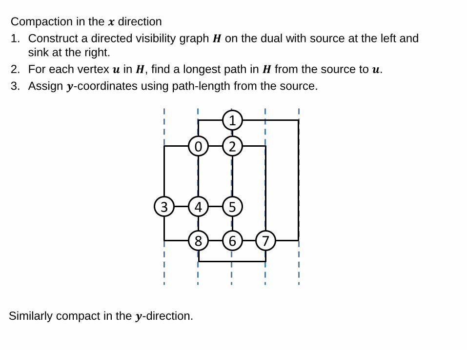
Compaction in the 𝒙 direction
1. Construct a directed visibility graph 𝑯 on the dual with source at the left and
sink at the right.
2. For each vertex 𝒖 in 𝑯, find a longest path in 𝑯 from the source to 𝒖.
3. Assign 𝒚-coordinates using path-length from the source.
5
2 0
1
8
3
7
4
6
Compaction in the 𝒙 direction
1. Construct a directed visibility graph 𝑯 on the dual with source at the left and
sink at the right.
2. For each vertex 𝒖 in 𝑯, find a longest path in 𝑯 from the source to 𝒖.
3. Assign 𝒚-coordinates using path-length from the source.
Similarly compact in the 𝒚-direction.
5
2 0
1
8
3
7
4
6

Remarks
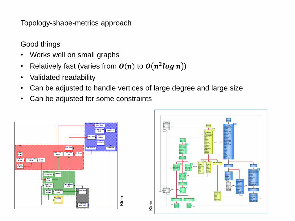
Topology-shape-metrics approach
Good things
• Works well on small graphs
• Relatively fast (varies from 𝑶(𝒏) to 𝑶 𝒏𝟐𝒍𝒐𝒈 𝒏 )
• Validated readability
• Can be adjusted to handle vertices of large degree and large size
• Can be adjusted for some constraints
Kle
in
Kle
in
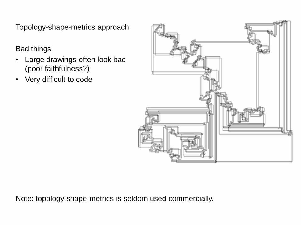
Topology-shape-metrics approach
Bad things
• Large drawings often look bad
(poor faithfulness?)
• Very difficult to code
Note: topology-shape-metrics is seldom used commercially.