Grammaticality and Lexical Statistics in Chinese Unnatural Phonotactics*

Donald Shuxiao Gong

Abstract

Speakers possess phonotactic knowledge about the acceptability of non-words, yet the source of this knowledge is not clear. Statistical analyses on a Chinese non-word judgement experiment have shown that both lexical statistics (neighbourhood density and Phonotactic Learner) and grammaticality (phonetically principled phonotactic constraints) play a role in predicting speakers’ behaviours. The results also indicate that a specific phonotactic constraint which bans Labial fricative to co-occur with Coronal glide (*[fj]) is well learned and noticed by speakers, despite its phonetic unnaturalness, suggesting that unnatural patterns are not necessarily dispreferred and underlearned. Keywords: Phonotactics, Lexical Statistics, Naturalness, Neighbourhood Density, Chinese

1 Introduction

Segments do not randomly combine with each other to form a word. There are certain constraints which place restrictions on the ability of certain types of segments to occur next to one another, which is known as phonotactics. A range of studies has confirmed that language speakers possess such phonotactic knowledge, because they offer gradient acceptability to non-words (Albright, 2009; A. Coetzee, 2008; Frisch & Zawaydeh, 2001; Hay, Pierrehumbert, & Beckman, 2003; Hayes & White, 2013). For example, although all missing from the real lexicon, English speakers will most probably judge blick as a highly possible word, while bnick is impossible, and lbick as completely unacceptable. What is less clear is the source of this phonotactic knowledge. One interpretation would be that speakers’ performance is guided by phonological grammar. To use the above example again, lbick is unacceptable because its onset cluster violates Sonority Sequencing Principle, a general preference of large rises in sonority from syllable edge to nucleus. Another theory contributes phonotactic knowledge to usage-based frequencies, i.e., lexical statistics. In this case, bnick and lbick are dispreferred because the onset sequence bn and lb are not well supported by the lexicon (in fact, the probability for bn and lb to occur word-initially is zero). Sometimes it is hard to disentangle these two, as ungrammatical forms may also lack lexical attestedness, and vice versa. A combinatory view would say that phonotactic knowledge is influenced by lexical statistics, while grammar still plays independent role (A. Coetzee, 2008). This paper uses data from Chinese to test these possibilities.

Chinese languages are often claimed to have a simple and restrictive syllable structure, and the most widely accepted model is CGVX (Duanmu, 2007). Despite the fact that Chinese is very strict about what sounds can occur with what, one puzzling question still remains: why there are so many theoretically possible syllables missing from the real inventory? According to Duanmu (2011)’s statistics, in Standard Chinese (SC), among all 1,900 possible syllables, only 404 are found; 79% of the syllable positions are missing. Many attempts have been made

*This paper would not have been completed without the supervision from James White. Thanks to James Myers for sharing the data and detailed discussion on neighbourhood density and Phonotactic Learner. Besides, thanks to Chulong Liu for his moral support in my dark days. Thanks to Yilei Shen, who is willing to reassure me on a daily basis. Finally, this paper is dedicated to YL.

UCLWPL 2017 2

to explain this large number of syllable gaps (Duanmu, 1990, 2003, 2007, 2008; Lin, 1989; Myers, 1995; Wiese, 1997), mainly based on feature co-occurrence or feature harmony. These attempts can be known as natural phonotactic constraints, as they all fall into some phonetic principles such as similarity avoidance (dissimilation). Syllables ruled out by such principled phonotactic constraints are classified as systematic gaps, whereas remaining missing forms are called accidental gaps (Halle, 1962). However, languages often present phonotactic constraints which will strike phonologists as being unnatural, or making no phonetic sense. For example, in SC, all labials can combine with the glide [j] except [f], that is, [pj] [phj] [mj] but *[fj]. This disfavour of [f] following a high front vocoid is also found in other Chinese languages such as Wu, Cantonese, Hakka, Xiang, and Gan. This constraint is considered as unnatural, or phonetically unmotivated at least, because there is no sensible phonetic grounding. There might be co-occurrence constraint on Labial onset and Labial glide, as the feature [Lab] cannot occur twice in sequence. However, a Labial onset is expected to freely host a Coronal glide [j], as [fj] does occur in many languages such as English. This paper will discuss speaker’s distinct performance regarding natural vs. unnatural phonotactic constraints.

Many theories believe that grammar is biased towards phonetic naturalness. One strong argument comes from Becker et al. (2007, 2011), showing that Turkish speakers are unable to generalise certain unnatural patterns exhibited in their lexicon. Turkish laryngeal alternation can partly be predicted by the place of articulation of the stem-final stop, by word-length, and by the preceding vowel quality. However, in novel word tasks, the productivity of this laryngeal alternation is only affected by place of articulation and word-length. Speakers tend to ignore the vowel quality effect, even though this information is provided by the lexicon. This finding is questioned by Hayes et al. (2009), claiming that an unnatural vowel harmony pattern in Turkish is learnable, but dispreferred. They in turn propose a biased Universal Grammar view: leaning a natural pattern is easier than an unnatural one (Hayes & White, 2013; Pater & Tessier, 2005; Pycha, Nowak, Shin, & Shosted, 2003; Wilson, 2003, 2006). Under this view, UG is linked with phonetic naturalness, and forms that violate natural phonotactic constraints are predicted to receive lower scores than those violating unnatural ones in non-word acceptability judgements. Quantitatively, the number of systematic gaps largely exceeds the accidental ones in Chinese syllabaries. However, intuitively, some accidental gaps mentioned above are in fact much less ‘accidental’ than they should be. First, they are not necessarily judged as more acceptable than systematic gaps (Myers, 2002). Second, those unnatural phonotactic constraints may recur in various Chinese languages. Why do such unnatural phonotactics exists?

Although a widely held assumption is that phonology should be phonetically grounded, synchronic phonology does allow a large number of unnatural patterns to occur (Anderson, 1981; Blevins, 2004). Contrary to the belief that phonology is shaped and determined by phonetic substance, Evolutionary Phonology leaves all such phonetic information to diachronic sound change; synchronic phonologies cannot refer to any phonetic details (Blevins, 2004). Many synchronic phonological rules make no phonetic sense, labelled as ‘crazy rules’ (Bach & Harms, 1972). Johnsen (2012) uses diachronic model to explain a synchronically unnatural retroflection pattern in Norwegian. A similar method is also adopted on a synchronic ‘crazy’ yet very productive rule of Sardinian (Scheer, 2015). The surface [l] → [ʁ] alternation is completely unnatural. Nevertheless, based on diachronic evidence and dialectal variation, this rule can be broken down as [l] → [ɫ] → [w] → [ɡʷ] → [ɣʷ] → [ʁ], with each step being grounded by phonetics. Phonotactic constraints which operate against phonetic naturalness are found in languages such as Tswana, Tarma Quechua and Berawan, where the phonetically more marked voiceless rather than voiced stops occur after a nasal or intervocalically, showing a post-nasal devoicing effect (Begus & Nazarov, 2017; A. W. Coetzee & Pretorius, 2010; Hyman, 2001). Kawahara (2008) also reports that in Japanese,

UCLWPL 2017 3

natural and unnatural patterns can co-occur in a single module of phonological grammar. Thus, synchronic unnaturalness can be explained by diachronic rule telescoping, and has a chance to enter speaker’s grammar. In some cases, unnatural constraints may even be over-phonologised by speakers. Kager & Pater (2012) find that the Dutch lexicon contains very few sequences of a long vowel followed by a consonant cluster whose second member is a non-coronal. This pattern is too complicated to be phonetically natural, yet speakers presented special sensitivity to it in well-formedness judgement tasks. Kirby & Yu (2007)’s well-formedness judgement data show that Cantonese speakers marked the nonce forms violating an unnatural Consonant-Vowel Coronal co-occurrence condition as less acceptable than forms violating a much more natural Labial co-occurrence restriction on Onsets and Codas. It seems that unnatural patterns can be productively internalised by native speakers, at least on an inductive basis.

This paper discusses the role of unnatural phonotactic constraints in Standard Chinese. Are they simply unimportant lexical accidents (badly supported by lexical statistics), or are they implicitly known by speakers and thus belong to the grammar? Section 2 discusses the restrictive syllabary of Standard Chinese and its natural and unnatural phonotactic constraints. Section 3 reviews the current debate on the source of natural vs. unnatural patterns. Section 4 presents statistical analyses of the data extracted from a huge Chinese non-word judgement experiment conducted by Myers & Tsay (2015), using lexical frequency and grammaticality parameters to predict participants’ reaction time and lexical decisions. Section 0 offers a discussion about the results, showing that besides lexical statistics, formal grammaticality has independent influence on linguistic performance. More importantly, an unnatural phonotactic constraint exhibits similar behaviour as other natural ones. Finally, Section 6 concludes.

2 Chinese Phonotactics 2.1 Systematic Gaps vs. Accidental Gaps

Due to a highly restrictive CGVX syllable structure (Duanmu, 2007), it is feasible to work out a list of theoretically possible syllables by factorial combination of all phonemes of the four syllable constituents. Here C stands for onset consonant, G for glide, V for nuclear vowel, and X for either an off-glide or a nasal coda. Taking SC as an example, the phoneme inventory of SC is shown below:

(1) Standard Chinese Phoneme Inventory C: p pʰ m f t tʰ n l ts tsʰ s tʂ tʂʰ ʂ ʐ k kʰ x G: j w ɥ V: a ə i u y X: i u n ŋ

In CGVX template, only the nuclear vowel V is obligatory, whereas other three constituents are optional. This gives rise to (18+1) × (3+1) × 5 × (4+1) = 1,900 theoretically possible syllables in SC, among which only 404 syllables actually occur. Syllabic consonant rhymes such as [z̩ n̩] and other unproductive rhymes like [ɚ] will be ignored.

Also, if we take tonal contrasts into consideration, there will be 1,900 × 4 = 7,600 distinct forms. However, I omit the discussion of tonal distinction here due to the following reasons. First, experimental results suggest that tonal accidental gaps are judged much more acceptable than other segmental gaps (Kirby & Yu, 2007; Myers, 2002; H. S. Wang, 1998). Second, other psycholinguistic studies show that tones are less important than previously assumed in language processing (e.g. Taft & Chen, 1992; Ye & Connine, 1999). For example,

UCLWPL 2017 4

when presented with non-words and asked to change them into real words by substituting a vowel, a consonant, or its lexical tone, speakers’ responses show that changes to vowels and consonants were more detrimental than tonal change, suggesting that tonal information is of lower priority than consonants and vowels (Wiener & Turnbull, 2016). Third, many tonal gaps are merely due to historical sound change. They are ubiquitous in other dialects and can be easily filled in by loan words, neologism, syllable combination in fast speech, and onomatopoetic words. Fourth, as we will see, tonal gaps often will not violate the principle phonotactic constraints we propose, if well defined. Tonal features are perceptually less salient than other segmental features. Thus, to avoid too much elaboration, tonal contrasts will not be considered.

Comparing theoretically possible syllables with actual existing syllables, we obtain a list of missing syllables. As mentioned in Section 1, the number of missing syllables is extremely high (1,496 for SC), and raises much theoretical attention on how to explain these missing forms. If we look at the syllable table, some patterns of those missing syllables can be immediately determined. For example, labial consonants [p ph m f] cannot co-occur with a labial glide [w], which leaves a huge blank in the syllable table. In the meantime, there are some sporadic, accidental gaps, such as *[fai] and [ʐai]: the rhyme [ai] can co-occur with all other 16 onsets except for [f] and [ʐ]. However, there is no consensus on how to treat these two types of syllable gaps, not only for SC, but also for other languages in general. Some believe that there is categorical distinction between the two, while others do not draw a clear line (Boersma & Hayes, 2001). However, much effort still has been made to figure out the phonological constraints on missing syllables, as stated in Coetzee (2008):

What is required is a way to distinguish between accidental lexical gaps and principled lexical gaps. It is not easy to formalize a principle that can be used for this purpose. However, as a first approximation I suggest the following: lexical gaps that can be stated in terms of general phonological properties should be treated as principled.

Similar arguments are provided in Frisch & Zawaydeh (2001). Indeed, efforts searching for phonotactic constraints turn out to be very successful, at least in Chinese languages. For example, Duanmu & Yi (2015) use only four constraints to explain 90% of the missing syllables in Lanzhou Mandarin. However, one must remain wary about the term “general phonological properties”, as it may still seem ambiguous and uncertain. Therefore, a clearer definition on the distinction between systematic gaps and accidental gaps is needed, yet we cannot ignore the descriptive power of the phonotactic constraints proposed for various languages.

Following Coetzee (2008)’s proposal, I use Standard Chinese as an example to show how natural (principled) phonotactic constraints help to distinguish systematic gaps and accidental gaps. Kessler & Treiman (1997) find that in English, onset-vowel combinations are statistically random, while vowel-coda sequences may be either underrepresented or overrepresented. This provides evidence for rhyme as a concrete syllable constituent, instead of nucleus and coda being independent units. Sinologists employ a traditional initial-final analysis for the study of Chinese phonology. Under this traditional method, glide is grouped as a rhyme constituent instead of onset (H Samuel Wang & Chang, 2001). The phonological system of fanqie was based on grouping glides with rhymes. Basically, fanqie method was a guideline to show the pronunciation of Chinese characters in Middle Chinese, widely used in ancient Chinese phonology books. It uses two characters to represent the pronunciation of a syllable for a new character. For example, the syllable [duŋ] is represented by [dɤ] + [huŋ], taking the onset of the first syllable and the rhyme of the second. When it comes to syllables

UCLWPL 2017 5

with prenuclear glides, the glide is usually parsed with the second syllable, meaning that the glide is not part of the onset. For instance, [du] + [njɛn] will give the pronunciation of [djɛn].

Here we adopt a similar method, by first considering missing rhymes, i.e., missing GVX forms, and then looking at missing onset-rhyme combinations, i.e., missing syllables.1 One missing rhyme is equivalent to 19 missing syllables, since each missing rhyme indicates that it cannot be combined with any onset consonant. Duanmu (2007) proposes three constraints, namely Rhyme Harmony, Merge, and G-Spreading, to account for the missing GVX forms in SC.

(2) Duanmu (2007)’s constraints a.

Rhyme Harmony: VX cannot have opposite values in [round] or [back], e.g. *[yi], *[yu]

b. Merge: Two tokens of the same feature merge into one long feature, e.g. [ii] = [i] c. G-Spreading: A high nuclear vowel spreads to the glide G, e.g. [u] = [wu]

However, this proposal is not satisfactory. First, some good forms, such as [iŋ] [un], are mistakenly ruled out, because he analyses [ŋ] and [n] as [+back] and [-back]. Second, this analysis leaves too many gaps as accidental: 23 GVX forms in number. The current analysis also proposes three constraints, adapted from Lin (1989) and Duanmu & Yi (2015). (3) Standard Chinese Rhyme Constraints a. * HH: The feature [+high] cannot occur in sequence. b. * [Cor]_[Cor]: [Cor] cannot occur in both G and X. c. * [Lab]_[Lab]: [Lab] cannot occur in both G and X. These three constraints can rule out most missing GVX forms, leaving only seven as accidental gaps: /ɥa ɥaŋ ɥən ɥəŋ un jən jəŋ/.2

As for Onset-Rhyme combinations, one simple constraint can explain most missing forms.

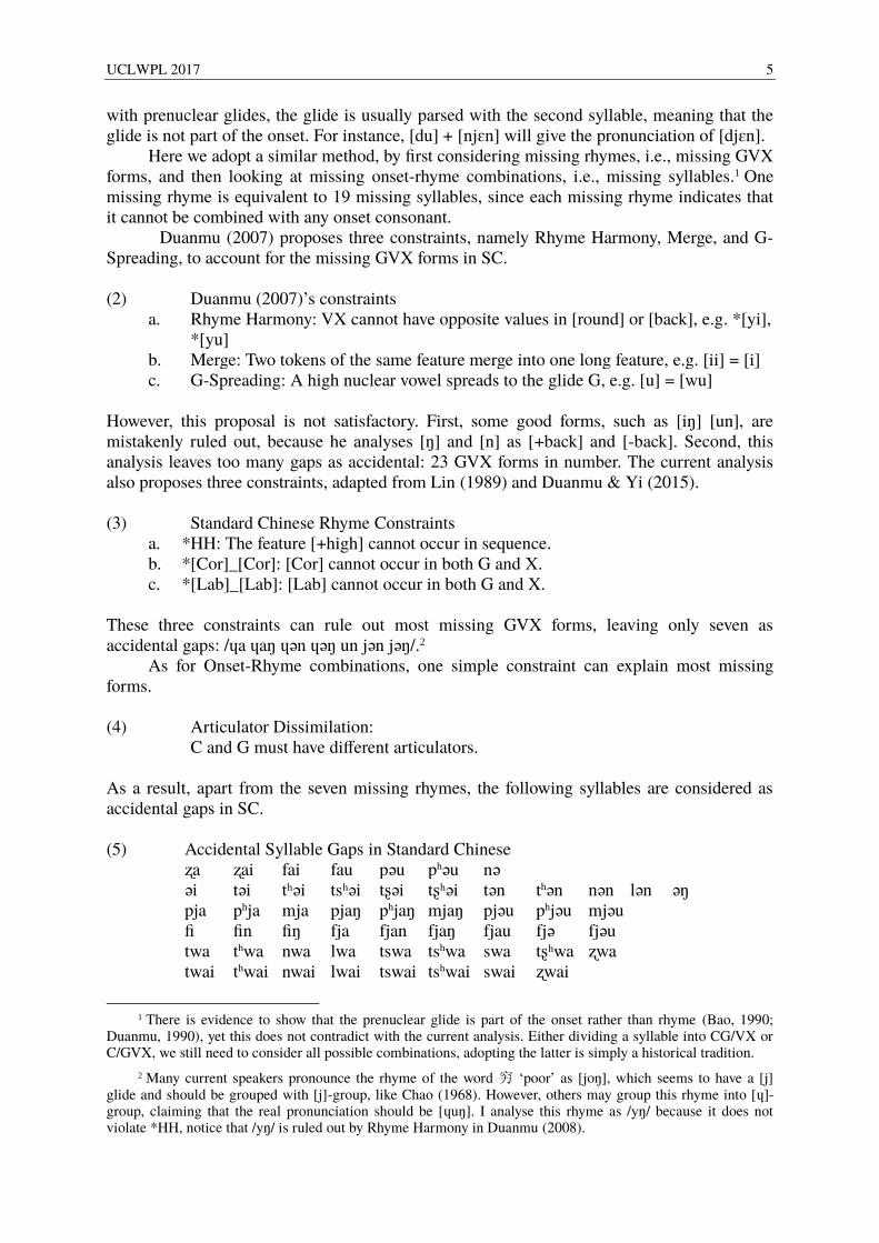
(4) Articulator Dissimilation: C and G must have different articulators. As a result, apart from the seven missing rhymes, the following syllables are considered as accidental gaps in SC. (5) Accidental Syllable Gaps in Standard Chinese ʐa ʐai fai fau pəu phəu nə əi təi tʰəi tsʰəi tʂəi tʂʰəi tən thən nən lən əŋ pja phja mja pjaŋ phjaŋ mjaŋ pjəu phjəu mjəu fi fin fiŋ fja fjan fjaŋ fjau fjə fjəu twa thwa nwa lwa tswa tshwa swa tʂʰwa ʐwa twai thwai nwai lwai tswai tshwai swai ʐwai

1 There is evidence to show that the prenuclear glide is part of the onset rather than rhyme (Bao, 1990;

Duanmu, 1990), yet this does not contradict with the current analysis. Either dividing a syllable into CG/VX or C/GVX, we still need to consider all possible combinations, adopting the latter is simply a historical tradition.

2 Many current speakers pronounce the rhyme of the word 穷 ‘poor’ as [joŋ], which seems to have a [j] glide and should be grouped with [j]-group, like Chao (1968). However, others may group this rhyme into [ɥ]-group, claiming that the real pronunciation should be [ɥuŋ]. I analyse this rhyme as /yŋ/ because it does not violate *HH, notice that /yŋ/ is ruled out by Rhyme Harmony in Duanmu (2008).

UCLWPL 2017 6

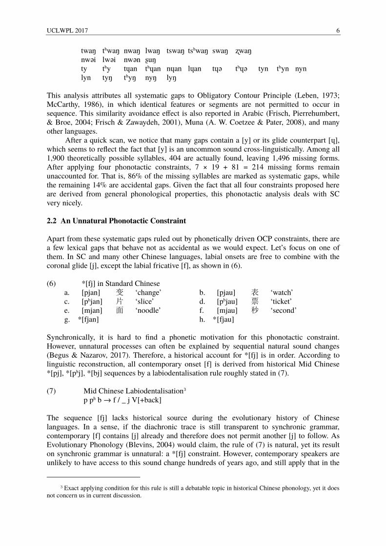
twaŋ thwaŋ nwaŋ lwaŋ tswaŋ tshwaŋ swaŋ ʐwaŋ nwəi lwəi nwən ʂuŋ ty thy tɥan thɥan nɥan lɥan tɥə thɥə tyn thyn nyn lyn tyŋ thyŋ nyŋ lyŋ This analysis attributes all systematic gaps to Obligatory Contour Principle (Leben, 1973; McCarthy, 1986), in which identical features or segments are not permitted to occur in sequence. This similarity avoidance effect is also reported in Arabic (Frisch, Pierrehumbert, & Broe, 2004; Frisch & Zawaydeh, 2001), Muna (A. W. Coetzee & Pater, 2008), and many other languages.

After a quick scan, we notice that many gaps contain a [y] or its glide counterpart [ɥ], which seems to reflect the fact that [y] is an uncommon sound cross-linguistically. Among all 1,900 theoretically possible syllables, 404 are actually found, leaving 1,496 missing forms. After applying four phonotactic constraints, 7 × 19 + 81 = 214 missing forms remain unaccounted for. That is, 86% of the missing syllables are marked as systematic gaps, while the remaining 14% are accidental gaps. Given the fact that all four constraints proposed here are derived from general phonological properties, this phonotactic analysis deals with SC very nicely.

2.2 An Unnatural Phonotactic Constraint Apart from these systematic gaps ruled out by phonetically driven OCP constraints, there are a few lexical gaps that behave not as accidental as we would expect. Let’s focus on one of them. In SC and many other Chinese languages, labial onsets are free to combine with the coronal glide [j], except the labial fricative [f], as shown in (6).

(6) *[fj] in Standard Chinese a. [pjan] 变 ‘change’ b. [pjau] 表 ‘watch’ c. [phjan] 片 ‘slice’ d. [phjau] 票 ‘ticket’ e. [mjan] 面 ‘noodle’ f. [mjau] 秒 ‘second’ g. * [fjan] h. * [fjau]

Synchronically, it is hard to find a phonetic motivation for this phonotactic constraint. However, unnatural processes can often be explained by sequential natural sound changes (Begus & Nazarov, 2017). Therefore, a historical account for *[fj] is in order. According to linguistic reconstruction, all contemporary onset [f] is derived from historical Mid Chinese *[pj], *[phj], *[bj] sequences by a labiodentalisation rule roughly stated in (7). (7) Mid Chinese Labiodentalisation3 p ph b → f / _ j V[+back]

The sequence [fj] lacks historical source during the evolutionary history of Chinese languages. In a sense, if the diachronic trace is still transparent to synchronic grammar, contemporary [f] contains [j] already and therefore does not permit another [j] to follow. As Evolutionary Phonology (Blevins, 2004) would claim, the rule of (7) is natural, yet its result on synchronic grammar is unnatural: a *[fj] constraint. However, contemporary speakers are unlikely to have access to this sound change hundreds of years ago, and still apply that in the

3 Exact applying condition for this rule is still a debatable topic in historical Chinese phonology, yet it does not concern us in current discussion.

UCLWPL 2017 7

grammar. Thus, a more possible hypothesis is that speakers are aware of this pattern, but in a synchronic way; any historical information is opaque.

On the other hand, there is a possibility that the acoustic properties of [fj] sequence is perceptually less salient; therefore speakers tend to avoid such sequence to occur in the lexicon. This would suggest that a constraint like *[fj] is phonetically natural. The details of such perceptual deficiencies are worth further investigation.

3 How to Treat Accidental Gaps 3.1 The Role of Naturalness Speakers’ judgements on non-words are gradient (Albright, 2009; Berent, Lennertz, Smolensky, & Vaknin-Nusbaum, 2009; Berent, Steriade, Lennertz, & Vaknin, 2007; Chomsky & Halle, 1965; A. Coetzee, 2008). Many would assume that systematic gaps will be marked as less acceptable in wug tests (Berko, 1958), and indeed this is reported in gradient acceptability experiments on English (A. W. Coetzee, 2009). This is because the syllable inventory of English is fuzzy; speakers do not have a clear distinction between words and non-words. Anecdotally, for Chinese, due to its small syllable inventory, native speakers are very sensitive to word/non-word distinction. One would expect that Chinese speakers will behave less gradiently and simply judge all non-words as equally unacceptable. However, previous acceptability experiments demonstrate that apparent accidental gaps are judged better than other apparent systematic gaps (Myers, 2002; Myers & Tsay, 2005; H. S. Wang, 1998), suggesting that even in Chinese, non-word judgement is gradient. Accidental gaps are supposed to be rated more highly than systematic gaps.

Nonetheless, some may argue that there is no clear-cut distinction among systematic and accidental gaps (Boersma & Hayes, 2001; Frisch, Large, & Pisoni, 2000). Things might become trickier when extending this type of analysis on other languages with less restrictive syllable structure and constituency, e.g. English. This is probably why no comprehensive analysis of English phonotactic constraints is available (but see Hayes (2012) for an attempt). It is not feasible to cope with so many phoneme slots and choices. Alternatively, computational phonotactic learner is developed to automatically figure out phonotactic constraints based on MaxEnt Grammar, by feeding lexicon data and the feature matrix (Hayes & Wilson, 2008). However, machine-learned constraints show some interesting patterns. Besides those would have been proposed by human linguists, the model also learns many constraints that make no phonological sense. For example, Hayes & Wilson’s model learns a constraint *[+round, +high][-cons, -son] for English, which seems completely unnatural in both phonetic and phonological sense (Hayes & White, 2013).

Phonotactic constraints can be subdivided into natural vs. unnatural ones, each playing distinct roles in phonological grammar. Return to our discussion of SC. If we study the missing syllables in more detail, we can propose more fine-grained and ad-hoc constraints, say, *[Cor, -cont][ən], which is a true reflection of the lexicon. Hayes et al. (2009) have shown that such detailed unnatural constraints are noticed by the speakers and they would make use of them in wug tests. However, it is unlikely to treat them as principled phonotactic constraints. According to Hayes & White (2013), phonotactic constraints should either be typologically well-attested or phonetically-grounded. The detailed constraints often meet neither of the criteria and thus should be marked as unnatural. Very often these unnatural phonotactics show ‘surfeit of the stimulus’ effect: despite being statistically significant in the lexicon, speakers tend to not generalise these unnatural phonotactic trends into nonce words. Synchronic approaches such as Phonetically Based Phonology (e.g. Hyman 2001; Hayes et al. 2004) would claim that cognitive system is prone to learn natural interactions. Unnatural

UCLWPL 2017 8

processes such as these unnatural phonotactic constraints cannot enter synchronic grammar (Becker, Eby Clemens, & Nevins, 2017; Becker et al., 2011; Becker, Nevins, & Levine, 2012; Pycha et al., 2003), or, at least natural processes are favoured by acquisition while unnatural patterns require extra intention to learn (Hayes et al., 2009; Hayes & White, 2013; Wilson, 2006). Meanwhile, detailed constraints only work for very few missing syllables. Hayes & Wilson’s model employs a generality heuristic when searching for phonotactic constraints: priority is given to the constraints which are able to cover a large portion of possible forms. In sum, the above studies suggest that phonetically natural constraints are psychologically real, whereas unnatural constraints are dispreferred and less noticed by speakers. I call this argument the naturalness view.

However, it also seems unfair to ignore all unnatural constraints. Some phonetically justified constraints may have lexical exceptions, lacking systematicity, and speakers may not even notice such constraints. For instance, there is a curious gap in SC: syllables both begin and end with a Coronal sound are disfavoured when the nuclear vowel is high front or mid. This appears to be a long-distance OCP effect. However, this constraint has several lexical exceptions, e.g. [lei, nen, lin] etc. Despite its naturalness, there is no evidence that native speakers will judge these gaps to be more unacceptable than pure accidental gaps. On the other hand, some accidental gaps are more noticed by speakers, and speakers strongly resist such gaps to enter the lexicon. This can be exemplified by the restricted distribution of SC rhyme [ia]. In SC, this rhyme can occur alone, or after Coronal affricates, while it is missing after all other onsets. This gap is genuinely accidental, as Hayes & Wilson (2008)’s phonotactic learner generates 0 penalty scores for these gaps (i.e. completely acceptable as a real lexical item) and there is no obvious natural phonetic explanation for these constraints. However, non-word acceptability tests show that these gaps receive lower judgements than expected, behaving more like those systematic gaps ruled out by natural constraints (Myers, 2002).

Diachronic approach such as Ohala’s listener-based sound change model (Ohala, 1981) or Evolutionary Phonology (Blevins, 2004) would suggest that synchronic patterns came into existence as a consequence of a series of diachronic events, and each diachronic stage is fully grounded in phonetic sense, either articulatorily or perceptually. In this case, synchronically natural patterns are certainly expected, and synchronically unnatural patterns can be decomposed into series of natural sound changes. Unnatural processes, just as natural ones, all have a discernible historical explanation, and may retain their productivity. For example, an unnatural constraint is reported for English, which allows only coronal consonant to follow the diphthong /au/, that is, shout, town, but *laup or *lauk (Hammond, 1999). Though being unnatural, this constraint experiences a natural history: modern /au/ vowel derived from historical monophthong *[u:]. Further, velar and labial sounds after historical *[u:] often underwent lenition, e.g. [b] → [β], [ɡ] → [ɣ], and subsequently vocalised as part of preceding vowel. On the other hand, historical long vowel *[u:] was frequently shortened to short vowel [u] or merged with *[o:] before velars and labials. Each of these steps was unrelated and grounded by phonetic motivation, yet the result that only modern [au][Cor] patterns survive is accidental and may appear to be unnatural. Moreover, some unnatural constraints are recurrent across languages. If we accept synchronic approach, we would expect that unnatural patterns to be deteriorating among world languages. However, there is no evidence to support such declining tendency (Buckley, 2000). For instance, the specific constraint *[fj], which bans labial-dental fricative to occur with coronal glide, holds true for seven major Chinese languages. If unnatural constraints are dispreferred, it is hard to explain why this pattern is recurrent across languages. In addition, Myers (2002) finds that the acceptability of these unnatural gaps is even lower than the gaps ruled out by natural constraints. Unnatural phonotactics, or in this case, accidental gaps, have the potential to be noticed by speakers and

UCLWPL 2017 9

then probably be internalised as part of the phonological grammar, just as other natural constraints. There is a chance for over-phonologisation of unnatural constraints. This can be known as diachrony view.

3.2 The Role of Lexical Statistics Both naturalness and diachrony view acknowledge that phonotactic constraints are part of the grammar, and this grammar guides speakers’ judgements on non-words. However, another potential source for phonological patterns arises from frequency distribution. High frequency results in higher grammaticality (Frisch & Zawaydeh, 2001). It is also argued that structures frequently presented in the lexicon might be phonologised even without phonetic grounding (Bybee, 2001). Also, nonce-words containing well-attested clusters are perceived more acceptable than those with low-frequency or unattested clusters (Coleman & Pierrehumbert, 1997). Therefore, if certain forms are perceived as less acceptable, it may simply due to its lack of support from the lexicon, not due to grammatical naturalness or any lexical-external explanations. ‘Grammar’ thus becomes the cognitive organisation of one’s linguistic experience. If this view is taken to its extreme, one may argue that phonological grammar is a projection of lexical statistics (Hay et al., 2003; Ohala, 1986), or an analogy of the lexicon (Daelemans & van den Bosch, 2005). Myers (2002) finds that speakers’ judgements show no significant difference between systematic gaps and accidental gaps. Violations of apparent principled phonotactic constraints are treated the same as of language-specific ad-hoc constraints (contrary to the findings in the current study, as will be discussed below). This indicates that a grammatical approach to phonology might not be necessary; analogical approach may suffice to explain non-word judgement. Non-word repetition tasks investigating the acquisition of novel phonotactic constraints show that speakers learn those constraints from recent experience of the experimental lexicon, suggesting that phonological knowledge can be reduced to statistical knowledge of patterns instantiated in the lexicon (Daland et al., 2011; Dell, Reed, Adams, & Meyer, 2000; Onishi, Chambers, & Fisher, 2002).

Numerous studies have shown that non-word acceptability judgements are related with lexical statistics (Bailey & Hahn, 2001; Coleman & Pierrehumbert, 1997; Frisch et al., 2000; Hay et al., 2003; Vitevitch & Luce, 1999, 1998). Other than English, such lexical effect on non-word gradient acceptability is also found in SC (Myers & Tsay, 2005) and Cantonese (Kirby & Yu, 2007). Different models have been proposed to quantify this lexical influence. First, speakers may evaluate how similar the non-word is with other known words, which is known as Neighbourhood Density. This is defined as the number of words generated by substituting, deleting, or adding a single phoneme together with their summed frequency (Bailey & Hahn, 2001; Greenberg & Jenkins, 1964). For example, the form lat has abundant lexical neighbours in English (e.g. cat, lap), while zev has sparse neighbourhood density. Second, speakers may decompose a non-word into substrings and calculate the combinatory probability of the phonemes of each substring. This method is called Phonotactic Probability (Jusczyk & Luce, 1994; Vitevitch & Luce, 1998). A widely accepted way to calculate phonotactic probability is position-specific biphone probability (Vitevitch & Luce, 2004). Given a sequence st found in the third and fourth positions of a word in English, we need to first sum up the frequency of all English words that contain st as their third and fourth segments, and divide that by the frequency count of all words that contain biphones in third and fourth positions. These two factors are usually confounded. since both are derived from lexical frequencies, high value in one factor may cause the other factor to be high as well. Nevertheless, many studies have proved that phonotactic probability and neighbourhood density have distinct effect on acceptability judgement (Bailey & Hahn, 2001). Myers & Tsay (2005) demonstrate that phonotactic probability boosts lexical decision in both word and non-

UCLWPL 2017 10

word scenario, while neighbourhood density only shows positive effect in real words; in non-words the effect is negative. This suggests that phonotactic probability is more like a pre-lexical grammatical process, while neighbourhood density is closely connected to the lexicon. This study also indicates that phonotactic probability is always a facilitator in lexical processing, while neighbourhood density, sometimes, can exhibit inhibitory effect, as too many neighbours may slow down the process of locating lexical item. Generally, phonotactic probability and neighbourhood density are considered as non-grammatical effect in language processing, since they are directly derived from lexical statistics (Inkelas, Orgun, & Zoll, 1997). However, some argue that phonotactic probability involves phonological generalisation, and thus should be viewed as part of the grammar. For example, Albright (2009) proposes a feature-based model which generates biphone probability by calculations over combinations of natural classes. Hayes & Wilson (2008)’s Phonotactic Learner also employs phonological features to calculate the optimal phonotactic constraint set that maximises the probability of input lexical items. On the other hand, the role of neighbourhood density is much more analogical rather than grammatical, as it only measures the similarity of a form with other lexical words.

Thus, one can argue that gradient acceptability of the missing syllables is a direct consequence of lexical statistics. Those missing forms which contain highly probable segment sequences or, more generally, have denser lexical neighbours, will be marked as more acceptable. However, this approach often fails to compare the acceptability between two missing forms, say [dl] and [bz]. Both sequences are missing from English and therefore having low phonotactic probability and sparse neighbourhood density (Albright, 2009). In addition, lexical frequency account says very little about the naturalness bias. A missing form is more acceptable than another because it is more word-like, not because it is more natural, or more grammatical. Experimental results also indicate that formal grammatical constraints like OCP do affect acceptability judgements, even when neighbourhood density and phonotactic probability are controlled (A. Coetzee, 2008; Frisch & Zawaydeh, 2001). A compromise approach between pure frequency-based and pure formal-grammar is in order: learners use frequency information only at the initial stage of learning. After being familiar with a patterns, grammar sets apart from lexical statistics and is ready for independent evolvements (A. Coetzee, 2008).

3.3 Summary

So far, we have met two theoretical questions. First, how do speakers treat natural vs. unnatural patterns? Do they prefer natural forms relative to unnatural ones, as predicted by naturalness view? Or diachrony view is more likely, that unnatural patterns are treated the same, or sometimes, even psychologically more real than natural patterns? Various experiments have confirmed that natural constraints are preferred (e.g. Berent et al. 2007; Carpenter 2010). Therefore, it is reasonable to believe that natural constraints form part of the grammar, and indeed, all constraints proposed for SC phonotactics in (3) and (4) are natural. Much of the debate has been focusing on unnatural patterns. Becker et al. (2011) argue that they are unlearnable, while others propose for soft bias, saying that unnatural patterns do exert some effect in acquisition and performance, but they are dispreferred (Hayes et al., 2009; Hayes & White, 2013; Wilson, 2006). Yet there is also evidence to show that unnatural constraints are being noticed by speakers. For example, Kager & Pater (2012) provide experimental evidence that Dutch speakers are actively aware of a phonotactic constraint which is too complex to be natural. There is no evidence that language-specific ad-hoc constraints cannot be more psychologically real than natural ones.

UCLWPL 2017 11

Second, suppose that speakers have implicit knowledge about phonotactic constraints, either natural or unnatural, we are also interested in the nature of this knowledge, i.e. is it a grammatical effect, or it is generalised from lexical analogy? Maybe it is more likely to accept natural constraints as part of the grammar. However, are unnatural constraints also part of the grammar, acting like other natural, principled constraints, or they are just accidentally true, an analogical reflection of lexical statistics? Also, we are interested in whether all unnatural constraints behave the same, that is, receiving similar wordlikeness judgements? If not, is it purely due to lexical statistics? Or it is because certain unnatural constraints are more prominent than the others and therefore guide speakers’ performance in such judgements?

In order to test the source of unnatural phonotactics, this paper will focus on one specific constraint, *[fj], as mentioned earlier. There is no straightforward phonetic evidence to explain this constraint, yet this pattern is widely found across different Chinese languages.

4 Statistical Analyses 4.1 Hypotheses

To evaluate the role of unnatural phonotactic constraints, this study compares speakers’ wordlikeness judgement performance of *[fj] violating gaps with (i) systematic (i.e. natural) gaps, and (ii) other accidental (i.e. unnatural) gaps. Previous experimental studies have shown that speakers will be slower to reject a token as non-word if it is more well-formed (Berent, Shimron, & Vaknin, 2001). It is therefore hypothesised that *[fj] violating gaps receive less positive responses and are rejected more quickly by participants than other accidental gaps. This will confirm that *[fj] behaves less accidentally and is learned well as if it were a natural constraint. Furthermore, to test whether the variance in performance can be simply explained by trends of the lexicon, lexical statistics will be included in the model. Suppose that *[fj] indeed is an unnatural constraint, if *[fj] effect remains significant after taking lexical statistics into consideration, then at least some unnatural phonotactics can be internalised as part of the grammar, which favours the diachrony view. 4.2 Data Sources

This study draws data from a phonological acceptability judgement mega study run on 110 Mandarin native speakers (Myers & Tsay, 2015). All 3,274 theoretically possible but actually missing syllables that are representable under Zhuyin Fuhao system were presented to the participants in written stimuli to judge their acceptability. Each participant was required to judge all missing syllables. Since this study was conducted in Taiwan, the written stimuli were in the form of Zhuyin Fuhao symbols, a phonetic spelling system used in Taiwan, equivalent to Mainland China’s Pinyin. Participants were asked to judge each stimulus as ‘like Mandarin’, or ‘not like Mandarin’ by pressing keys on the keyboard as quickly as possible, and their response and reaction time were recorded. Even though SC speakers are said to possess a sharp intuition between words and non-words (Myers, 2002; H. S. Wang, 1998), 13.42% of all responses were positive despite the fact that all syllables presented to participants were non-words.

Not all missing syllables included in the original data are selected for current analysis. First, original data distinguish lexical tones of each missing syllable, which are merged in current study. For example, the missing syllable *[pja] is labelled as [pja1], [pja2], [pja3], [pja4] in the original dataset, and participants offer judgements to each of them. Now that lexical tones are merged, these four missing forms are treated as identical, yet their reaction times are preserved, as if participants judge [pja] for four times. This is true for all syllables

UCLWPL 2017 12

being considered so the tonal distinctions of reaction time are balanced across all syllables. Second, due to different phonemic analysis, many syllable forms in the original dataset are non-contrastive under the current phonemic analysis of (1), and therefore being eliminated from further consideration. For instance, ㄐㄜ [je] and ㄐㄛ [jo] are counted as different forms in Myers & Tsay (2015)’s missing syllable list. However, in fact, SC has only one mid vowel phoneme. The mid vowel /ə/ is realised as [e] after the glide [j], so [jo] is impossible and redundant. In other words, the constraints covered in this study are all morphophonotactic constraints which operate on the phonemic input segments, rather than surface phonetic output segments. After merging lexical tones and ruling out impossible forms, we identify 360 non-lexical syllables from the original 3,274.4 Among them, 128 syllables are labelled as accidental, and the remaining 232 are systematic gaps, i.e., ruled out by the constraints proposed in (3) and (4). Further, we label 12 *[fj] violating syllables out of all others as out theoretical interest group.

As mentioned before, non-word judgement data can be explained by lexical statistics. Two models have been introduced as the predictors for the reaction time variance in this study. The first one is Hayes & Wilson (2008)’s Maximum Entropy Phonotactic Learner, which is a constraint-based phonotactic learner producing a set of feature-based constraints given a feature matrix and a lexicon for training. The learner attempts to identify the constraint set and a set of constraint weights that maximise the probability of the input forms. The training lexicon is derived from Tsai (2000)’s Mandarin Syllable Frequency Counts for Chinese Characters. It iterates through the 111,417 words included in an online Chinese lexicon Libtabe (Hsiao, Tsai, Hsieh, Yeh, & Tan, 2013) and counts the frequency of occurrence for each pronunciation of each character. As a result, the frequency was type frequency. For example, if a character is pronounced "hui4" in 402 words in the lexicon, the frequency will be 402. The pronunciations with their frequencies are then merged with tones (by adding up the type frequencies of four lexical tones) and reinterpreted under the phonemic analysis in (1). In the end this generates a corpus of 399 lexical entries with type frequency. The feature definition of each segment follows the analysis in Duanmu (2007). The number of constraints to be learned is set as 400. After obtaining the constraint set, we apply this grammar to the testing data, which is the 360 non-lexical syllables mentioned earlier. Each missing syllable is thus assigned a penalty score to reflect its lexical well-formedness. The second lexical statistics predictor is Neighbourhood Density. We use the standard definition of Levenshtein Edit Distance, that is, by calculating the number of lexical neighbours differing in only one phoneme (either adding, deleting, or substituting) from the test item for all 360 non-lexical syllables (Luce & Pisoni, 1998). The corpus data is the same as the one used for Phonotactic Learner, and the searching algorithm is provided by Hall et al. (2017).

4.3 Results First, we use the independent variables to predict reaction time. Here we exclude the 13.42% of positive responses, since positive responses may be involved with a distinct processing pattern than of non-word judgement. The statistical analysis employs a powerful technique named mixed-effects linear regression (Baayen, Davidson, & Bates, 2008), which simultaneously incorporates random effects (the participants and test items) and fixed effects (in this case, our four independent predictors: penalty scores generated by phonotactic learner,

4 This number is different from 1,496 as discussed before. This is because Myers & Tsay (2015)’s data does not include any syllable violating *HH, since rhymes violating this constraint like [iu], [yi] cannot be represented by Zhuyin Fuhao system, and indeed a large number of missing syllables is under this constraint.

UCLWPL 2017 13

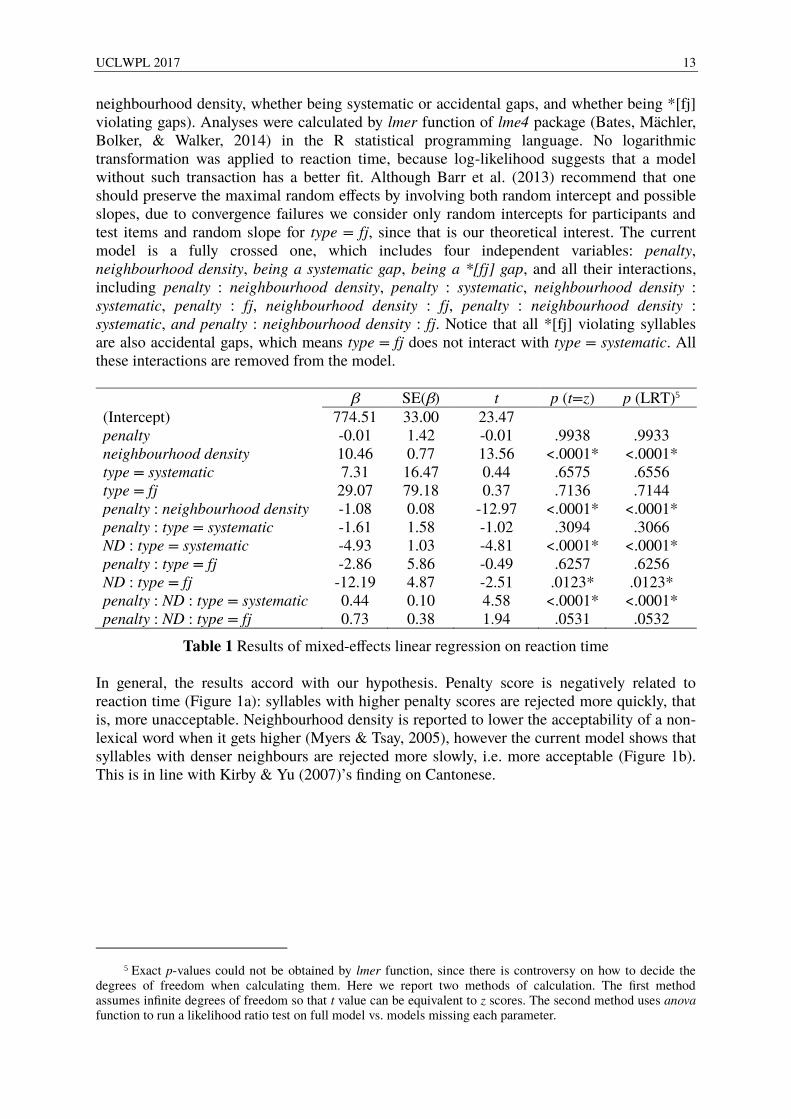
neighbourhood density, whether being systematic or accidental gaps, and whether being *[fj] violating gaps). Analyses were calculated by lmer function of lme4 package (Bates, Mächler, Bolker, & Walker, 2014) in the R statistical programming language. No logarithmic transformation was applied to reaction time, because log-likelihood suggests that a model without such transaction has a better fit. Although Barr et al. (2013) recommend that one should preserve the maximal random effects by involving both random intercept and possible slopes, due to convergence failures we consider only random intercepts for participants and test items and random slope for type = fj, since that is our theoretical interest. The current model is a fully crossed one, which includes four independent variables: penalty, neighbourhood density, being a systematic gap, being a *[fj] gap, and all their interactions, including penalty : neighbourhood density, penalty : systematic, neighbourhood density : systematic, penalty : fj, neighbourhood density : fj, penalty : neighbourhood density : systematic, and penalty : neighbourhood density : fj. Notice that all *[fj] violating syllables are also accidental gaps, which means type = fj does not interact with type = systematic. All these interactions are removed from the model. β SE(β) t p (t=z) p (LRT)5 (Intercept) 774.51 33.00 23.47 penalty -0.01 1.42 -0.01 .9938 .9933 neighbourhood density 10.46 0.77 13.56 <.0001* <.0001* type = systematic 7.31 16.47 0.44 .6575 .6556 type = fj 29.07 79.18 0.37 .7136 .7144 penalty : neighbourhood density -1.08 0.08 -12.97 <.0001* <.0001* penalty : type = systematic -1.61 1.58 -1.02 .3094 .3066 ND : type = systematic -4.93 1.03 -4.81 <.0001* <.0001* penalty : type = fj -2.86 5.86 -0.49 .6257 .6256 ND : type = fj -12.19 4.87 -2.51 .0123* .0123* penalty : ND : type = systematic 0.44 0.10 4.58 <.0001* <.0001* penalty : ND : type = fj 0.73 0.38 1.94 .0531 .0532

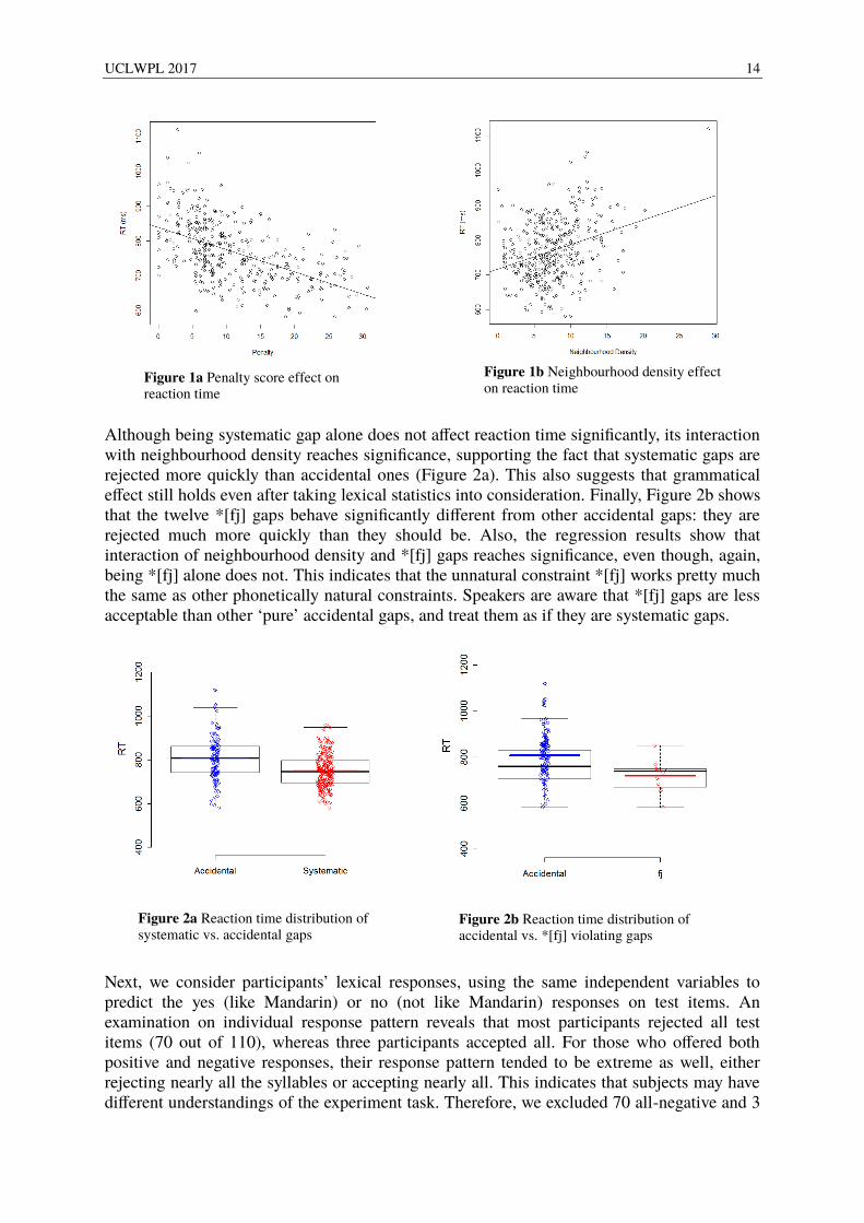
Table 1 Results of mixed-effects linear regression on reaction time In general, the results accord with our hypothesis. Penalty score is negatively related to reaction time (Figure 1a): syllables with higher penalty scores are rejected more quickly, that is, more unacceptable. Neighbourhood density is reported to lower the acceptability of a non-lexical word when it gets higher (Myers & Tsay, 2005), however the current model shows that syllables with denser neighbours are rejected more slowly, i.e. more acceptable (Figure 1b). This is in line with Kirby & Yu (2007)’s finding on Cantonese.

5 Exact p-values could not be obtained by lmer function, since there is controversy on how to decide the degrees of freedom when calculating them. Here we report two methods of calculation. The first method assumes infinite degrees of freedom so that t value can be equivalent to z scores. The second method uses anova function to run a likelihood ratio test on full model vs. models missing each parameter.

UCLWPL 2017 14

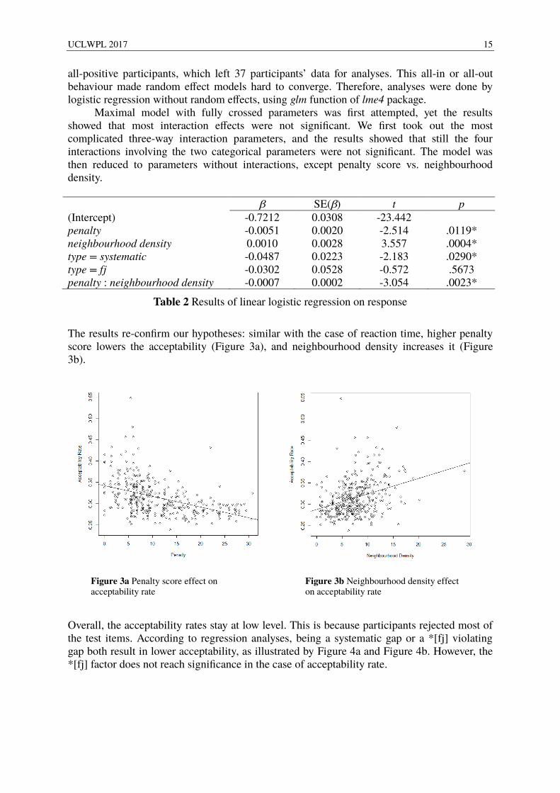
Although being systematic gap alone does not affect reaction time significantly, its interaction with neighbourhood density reaches significance, supporting the fact that systematic gaps are rejected more quickly than accidental ones (Figure 2a). This also suggests that grammatical effect still holds even after taking lexical statistics into consideration. Finally, Figure 2b shows that the twelve *[fj] gaps behave significantly different from other accidental gaps: they are rejected much more quickly than they should be. Also, the regression results show that interaction of neighbourhood density and *[fj] gaps reaches significance, even though, again, being *[fj] alone does not. This indicates that the unnatural constraint *[fj] works pretty much the same as other phonetically natural constraints. Speakers are aware that *[fj] gaps are less acceptable than other ‘pure’ accidental gaps, and treat them as if they are systematic gaps.

Next, we consider participants’ lexical responses, using the same independent variables to predict the yes (like Mandarin) or no (not like Mandarin) responses on test items. An examination on individual response pattern reveals that most participants rejected all test items (70 out of 110), whereas three participants accepted all. For those who offered both positive and negative responses, their response pattern tended to be extreme as well, either rejecting nearly all the syllables or accepting nearly all. This indicates that subjects may have different understandings of the experiment task. Therefore, we excluded 70 all-negative and 3

Figure 1a Penalty score effect on reaction time

Figure 1b Neighbourhood density effect on reaction time

Figure 2a Reaction time distribution of systematic vs. accidental gaps

Figure 2b Reaction time distribution of accidental vs. *[fj] violating gaps

UCLWPL 2017 15

all-positive participants, which left 37 participants’ data for analyses. This all-in or all-out behaviour made random effect models hard to converge. Therefore, analyses were done by logistic regression without random effects, using glm function of lme4 package.

Maximal model with fully crossed parameters was first attempted, yet the results showed that most interaction effects were not significant. We first took out the most complicated three-way interaction parameters, and the results showed that still the four interactions involving the two categorical parameters were not significant. The model was then reduced to parameters without interactions, except penalty score vs. neighbourhood density. β SE(β) t p (Intercept) -0.7212 0.0308 -23.442 penalty -0.0051 0.0020 -2.514 .0119* neighbourhood density 0.0010 0.0028 3.557 .0004* type = systematic -0.0487 0.0223 -2.183 .0290* type = fj -0.0302 0.0528 -0.572 .5673 penalty : neighbourhood density -0.0007 0.0002 -3.054 .0023*

Table 2 Results of linear logistic regression on response

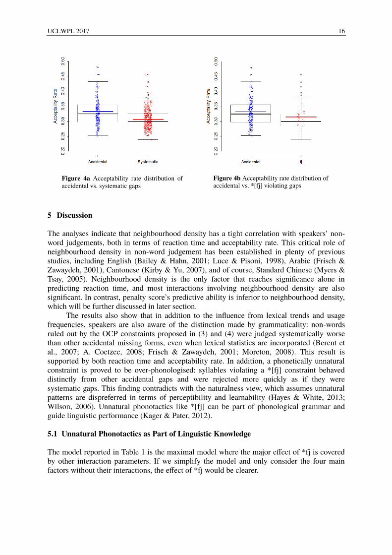
The results re-confirm our hypotheses: similar with the case of reaction time, higher penalty score lowers the acceptability (Figure 3a), and neighbourhood density increases it (Figure 3b).

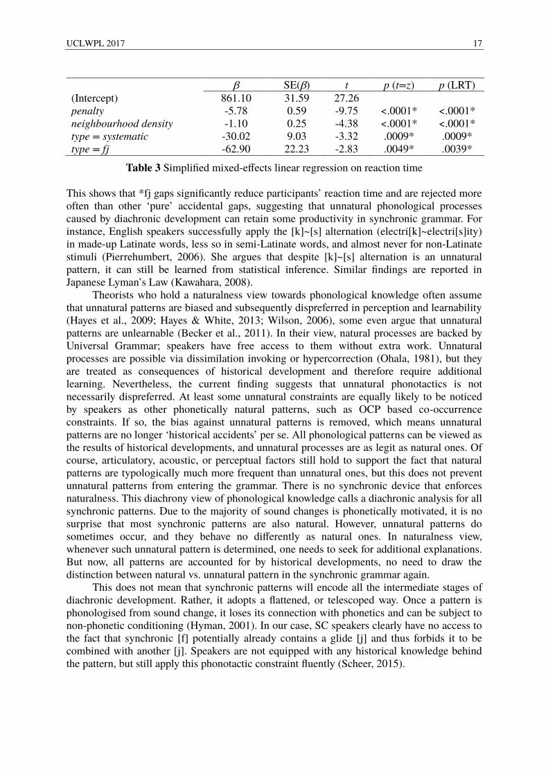
Overall, the acceptability rates stay at low level. This is because participants rejected most of the test items. According to regression analyses, being a systematic gap or a *[fj] violating gap both result in lower acceptability, as illustrated by Figure 4a and Figure 4b. However, the *[fj] factor does not reach significance in the case of acceptability rate.

Figure 3a Penalty score effect on acceptability rate

Figure 3b Neighbourhood density effect on acceptability rate

UCLWPL 2017 16

5 Discussion

The analyses indicate that neighbourhood density has a tight correlation with speakers’ non-word judgements, both in terms of reaction time and acceptability rate. This critical role of neighbourhood density in non-word judgement has been established in plenty of previous studies, including English (Bailey & Hahn, 2001; Luce & Pisoni, 1998), Arabic (Frisch & Zawaydeh, 2001), Cantonese (Kirby & Yu, 2007), and of course, Standard Chinese (Myers & Tsay, 2005). Neighbourhood density is the only factor that reaches significance alone in predicting reaction time, and most interactions involving neighbourhood density are also significant. In contrast, penalty score’s predictive ability is inferior to neighbourhood density, which will be further discussed in later section.

The results also show that in addition to the influence from lexical trends and usage frequencies, speakers are also aware of the distinction made by grammaticality: non-words ruled out by the OCP constraints proposed in (3) and (4) were judged systematically worse than other accidental missing forms, even when lexical statistics are incorporated (Berent et al., 2007; A. Coetzee, 2008; Frisch & Zawaydeh, 2001; Moreton, 2008). This result is supported by both reaction time and acceptability rate. In addition, a phonetically unnatural constraint is proved to be over-phonologised: syllables violating a *[fj] constraint behaved distinctly from other accidental gaps and were rejected more quickly as if they were systematic gaps. This finding contradicts with the naturalness view, which assumes unnatural patterns are dispreferred in terms of perceptibility and learnability (Hayes & White, 2013; Wilson, 2006). Unnatural phonotactics like *[fj] can be part of phonological grammar and guide linguistic performance (Kager & Pater, 2012).

5.1 Unnatural Phonotactics as Part of Linguistic Knowledge The model reported in Table 1 is the maximal model where the major effect of *fj is covered by other interaction parameters. If we simplify the model and only consider the four main factors without their interactions, the effect of *fj would be clearer.

Figure 4a Acceptability rate distribution of accidental vs. systematic gaps

Figure 4b Acceptability rate distribution of accidental vs. *[fj] violating gaps

UCLWPL 2017 17

β SE(β) t p (t=z) p (LRT) (Intercept) 861.10 31.59 27.26 penalty -5.78 0.59 -9.75 <.0001* <.0001* neighbourhood density -1.10 0.25 -4.38 <.0001* <.0001* type = systematic -30.02 9.03 -3.32 .0009* .0009* type = fj -62.90 22.23 -2.83 .0049* .0039*

Table 3 Simplified mixed-effects linear regression on reaction time This shows that *fj gaps significantly reduce participants’ reaction time and are rejected more often than other ‘pure’ accidental gaps, suggesting that unnatural phonological processes caused by diachronic development can retain some productivity in synchronic grammar. For instance, English speakers successfully apply the [k]~[s] alternation (electri[k]~electri[s]ity) in made-up Latinate words, less so in semi-Latinate words, and almost never for non-Latinate stimuli (Pierrehumbert, 2006). She argues that despite [k]~[s] alternation is an unnatural pattern, it can still be learned from statistical inference. Similar findings are reported in Japanese Lyman’s Law (Kawahara, 2008).

Theorists who hold a naturalness view towards phonological knowledge often assume that unnatural patterns are biased and subsequently dispreferred in perception and learnability (Hayes et al., 2009; Hayes & White, 2013; Wilson, 2006), some even argue that unnatural patterns are unlearnable (Becker et al., 2011). In their view, natural processes are backed by Universal Grammar; speakers have free access to them without extra work. Unnatural processes are possible via dissimilation invoking or hypercorrection (Ohala, 1981), but they are treated as consequences of historical development and therefore require additional learning. Nevertheless, the current finding suggests that unnatural phonotactics is not necessarily dispreferred. At least some unnatural constraints are equally likely to be noticed by speakers as other phonetically natural patterns, such as OCP based co-occurrence constraints. If so, the bias against unnatural patterns is removed, which means unnatural patterns are no longer ‘historical accidents’ per se. All phonological patterns can be viewed as the results of historical developments, and unnatural processes are as legit as natural ones. Of course, articulatory, acoustic, or perceptual factors still hold to support the fact that natural patterns are typologically much more frequent than unnatural ones, but this does not prevent unnatural patterns from entering the grammar. There is no synchronic device that enforces naturalness. This diachrony view of phonological knowledge calls a diachronic analysis for all synchronic patterns. Due to the majority of sound changes is phonetically motivated, it is no surprise that most synchronic patterns are also natural. However, unnatural patterns do sometimes occur, and they behave no differently as natural ones. In naturalness view, whenever such unnatural pattern is determined, one needs to seek for additional explanations. But now, all patterns are accounted for by historical developments, no need to draw the distinction between natural vs. unnatural pattern in the synchronic grammar again.

This does not mean that synchronic patterns will encode all the intermediate stages of diachronic development. Rather, it adopts a flattened, or telescoped way. Once a pattern is phonologised from sound change, it loses its connection with phonetics and can be subject to non-phonetic conditioning (Hyman, 2001). In our case, SC speakers clearly have no access to the fact that synchronic [f] potentially already contains a glide [j] and thus forbids it to be combined with another [j]. Speakers are not equipped with any historical knowledge behind the pattern, but still apply this phonotactic constraint fluently (Scheer, 2015).

UCLWPL 2017 18

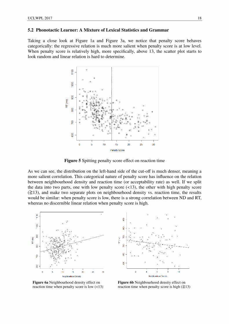
5.2 Phonotactic Learner: A Mixture of Lexical Statistics and Grammar Taking a close look at Figure 1a and Figure 3a, we notice that penalty score behaves categorically: the regressive relation is much more salient when penalty score is at low level. When penalty score is relatively high, more specifically, above 13, the scatter plot starts to look random and linear relation is hard to determine.

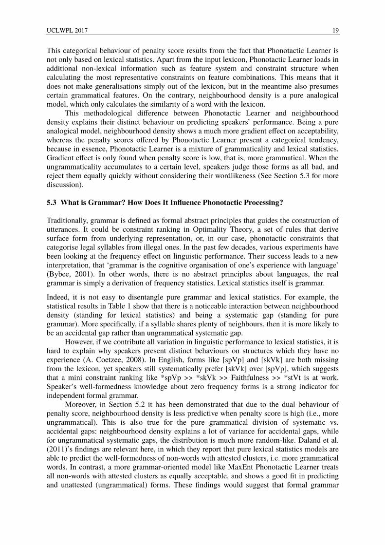
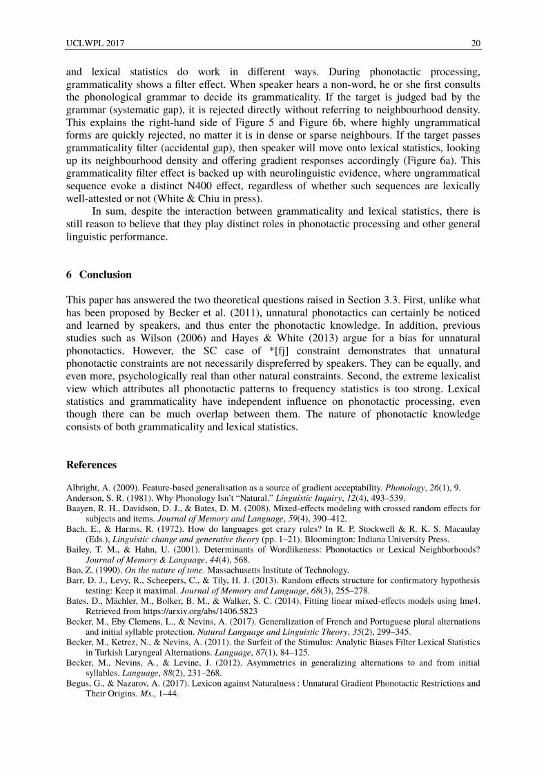
Figure 5 Spitting penalty score effect on reaction time As we can see, the distribution on the left-hand side of the cut-off is much denser, meaning a more salient correlation. This categorical nature of penalty score has influence on the relation between neighbourhood density and reaction time (or acceptability rate) as well. If we split the data into two parts, one with low penalty score (<13), the other with high penalty score (≧13), and make two separate plots on neighbourhood density vs. reaction time, the results would be similar: when penalty score is low, there is a strong correlation between ND and RT, whereas no discernible linear relation when penalty score is high.

Figure 6a Neighbourhood density effect on reaction time when penalty score is low (<13)

Figure 6b Neighbourhood density effect on reaction time when penalty score is high (≧13)

UCLWPL 2017 19

This categorical behaviour of penalty score results from the fact that Phonotactic Learner is not only based on lexical statistics. Apart from the input lexicon, Phonotactic Learner loads in additional non-lexical information such as feature system and constraint structure when calculating the most representative constraints on feature combinations. This means that it does not make generalisations simply out of the lexicon, but in the meantime also presumes certain grammatical features. On the contrary, neighbourhood density is a pure analogical model, which only calculates the similarity of a word with the lexicon.

This methodological difference between Phonotactic Learner and neighbourhood density explains their distinct behaviour on predicting speakers’ performance. Being a pure analogical model, neighbourhood density shows a much more gradient effect on acceptability, whereas the penalty scores offered by Phonotactic Learner present a categorical tendency, because in essence, Phonotactic Learner is a mixture of grammaticality and lexical statistics. Gradient effect is only found when penalty score is low, that is, more grammatical. When the ungrammaticality accumulates to a certain level, speakers judge those forms as all bad, and reject them equally quickly without considering their wordlikeness (See Section 5.3 for more discussion).

5.3 What is Grammar? How Does It Influence Phonotactic Processing? Traditionally, grammar is defined as formal abstract principles that guides the construction of utterances. It could be constraint ranking in Optimality Theory, a set of rules that derive surface form from underlying representation, or, in our case, phonotactic constraints that categorise legal syllables from illegal ones. In the past few decades, various experiments have been looking at the frequency effect on linguistic performance. Their success leads to a new interpretation, that ‘grammar is the cognitive organisation of one’s experience with language’ (Bybee, 2001). In other words, there is no abstract principles about languages, the real grammar is simply a derivation of frequency statistics. Lexical statistics itself is grammar.

Indeed, it is not easy to disentangle pure grammar and lexical statistics. For example, the statistical results in Table 1 show that there is a noticeable interaction between neighbourhood density (standing for lexical statistics) and being a systematic gap (standing for pure grammar). More specifically, if a syllable shares plenty of neighbours, then it is more likely to be an accidental gap rather than ungrammatical systematic gap.

However, if we contribute all variation in linguistic performance to lexical statistics, it is hard to explain why speakers present distinct behaviours on structures which they have no experience (A. Coetzee, 2008). In English, forms like [spVp] and [skVk] are both missing from the lexicon, yet speakers still systematically prefer [skVk] over [spVp], which suggests that a mini constraint ranking like *spVp >> *skVk >> Faithfulness >> *stVt is at work. Speaker’s well-formedness knowledge about zero frequency forms is a strong indicator for independent formal grammar.

Moreover, in Section 5.2 it has been demonstrated that due to the dual behaviour of penalty score, neighbourhood density is less predictive when penalty score is high (i.e., more ungrammatical). This is also true for the pure grammatical division of systematic vs. accidental gaps: neighbourhood density explains a lot of variance for accidental gaps, while for ungrammatical systematic gaps, the distribution is much more random-like. Daland et al. (2011)’s findings are relevant here, in which they report that pure lexical statistics models are able to predict the well-formedness of non-words with attested clusters, i.e. more grammatical words. In contrast, a more grammar-oriented model like MaxEnt Phonotactic Learner treats all non-words with attested clusters as equally acceptable, and shows a good fit in predicting and unattested (ungrammatical) forms. These findings would suggest that formal grammar

UCLWPL 2017 20

and lexical statistics do work in different ways. During phonotactic processing, grammaticality shows a filter effect. When speaker hears a non-word, he or she first consults the phonological grammar to decide its grammaticality. If the target is judged bad by the grammar (systematic gap), it is rejected directly without referring to neighbourhood density. This explains the right-hand side of Figure 5 and Figure 6b, where highly ungrammatical forms are quickly rejected, no matter it is in dense or sparse neighbours. If the target passes grammaticality filter (accidental gap), then speaker will move onto lexical statistics, looking up its neighbourhood density and offering gradient responses accordingly (Figure 6a). This grammaticality filter effect is backed up with neurolinguistic evidence, where ungrammatical sequence evoke a distinct N400 effect, regardless of whether such sequences are lexically well-attested or not (White & Chiu in press).

In sum, despite the interaction between grammaticality and lexical statistics, there is still reason to believe that they play distinct roles in phonotactic processing and other general linguistic performance.

6 Conclusion This paper has answered the two theoretical questions raised in Section 3.3. First, unlike what has been proposed by Becker et al. (2011), unnatural phonotactics can certainly be noticed and learned by speakers, and thus enter the phonotactic knowledge. In addition, previous studies such as Wilson (2006) and Hayes & White (2013) argue for a bias for unnatural phonotactics. However, the SC case of *[fj] constraint demonstrates that unnatural phonotactic constraints are not necessarily dispreferred by speakers. They can be equally, and even more, psychologically real than other natural constraints. Second, the extreme lexicalist view which attributes all phonotactic patterns to frequency statistics is too strong. Lexical statistics and grammaticality have independent influence on phonotactic processing, even though there can be much overlap between them. The nature of phonotactic knowledge consists of both grammaticality and lexical statistics. References Albright, A. (2009). Feature-based generalisation as a source of gradient acceptability. Phonology, 26(1), 9. Anderson, S. R. (1981). Why Phonology Isn’t “Natural.” Linguistic Inquiry, 12(4), 493–539. Baayen, R. H., Davidson, D. J., & Bates, D. M. (2008). Mixed-effects modeling with crossed random effects for

subjects and items. Journal of Memory and Language, 59(4), 390–412. Bach, E., & Harms, R. (1972). How do languages get crazy rules? In R. P. Stockwell & R. K. S. Macaulay

(Eds.), Linguistic change and generative theory (pp. 1–21). Bloomington: Indiana University Press. Bailey, T. M., & Hahn, U. (2001). Determinants of Wordlikeness: Phonotactics or Lexical Neighborhoods?

Journal of Memory & Language, 44(4), 568. Bao, Z. (1990). On the nature of tone. Massachusetts Institute of Technology. Barr, D. J., Levy, R., Scheepers, C., & Tily, H. J. (2013). Random effects structure for confirmatory hypothesis

testing: Keep it maximal. Journal of Memory and Language, 68(3), 255–278. Bates, D., Mächler, M., Bolker, B. M., & Walker, S. C. (2014). Fitting linear mixed-effects models using lme4.

Retrieved from https://arxiv.org/abs/1406.5823 Becker, M., Eby Clemens, L., & Nevins, A. (2017). Generalization of French and Portuguese plural alternations

and initial syllable protection. Natural Language and Linguistic Theory, 35(2), 299–345. Becker, M., Ketrez, N., & Nevins, A. (2011). the Surfeit of the Stimulus: Analytic Biases Filter Lexical Statistics

in Turkish Laryngeal Alternations. Language, 87(1), 84–125. Becker, M., Nevins, A., & Levine, J. (2012). Asymmetries in generalizing alternations to and from initial

syllables. Language, 88(2), 231–268. Begus, G., & Nazarov, A. (2017). Lexicon against Naturalness : Unnatural Gradient Phonotactic Restrictions and

Their Origins. Ms., 1–44.

UCLWPL 2017 21

Berent, I., Lennertz, T., Smolensky, P., & Vaknin-Nusbaum, V. (2009). Listeners’ knowledge of phonological universals: evidence from nasal clusters. Phonology, 26(1), 75.

Berent, I., Shimron, J., & Vaknin, V. (2001). Phonological Constraints on Reading: Evidence from the Obligatory Contour Principle. Journal of Memory and Language, 44(4), 644–665.

Berent, I., Steriade, D., Lennertz, T., & Vaknin, V. (2007). What we know about what we have never heard: Evidence from perceptual illusions. Cognition, 104(3), 591–630.

Berko, J. (1958). A child’s learning of English morphology. Word, 14(November), 150–77. Blevins, J. (2004). Evolutionary Phonology. Cambridge: Cambridge University Press. Boersma, P., & Hayes, B. (2001). Empirical Tests of the Gradual Learning Algorithm. Linguistic Inquiry, 32(1),

45–86. Buckley, E. (2000). On the Naturalness of Unnatural Rules. Proceedings from the Second Workshop on

American Indigenous Languages., 9, 1–14. Bybee, J. (2001). Phonology and language use. Cambridge: Cambridge University Press. Carpenter, A. C. (2010). A naturalness bias in learning stress. Phonology, 27(3), 345–392. Chao, Y.-R. (1968). A Grammar of Spoken Chinese. Berkeley and Los Angeles: University of California Press. Chomsky, N., & Halle, M. (1965). Some controversial questions in phonetical theory. Journal of Linguistics,

1(2), 97–138. Coetzee, A. (2008). Grammaticality and Ungrammaticality in Phonology. Language, 84(2), 218–257. Coetzee, A. W. (2009). Grammar is both categorical and gradient. Phonological Argumentation: Essays on

Evidence and Motivation, 1–36. Coetzee, A. W., & Pater, J. (2008). Weighted Constraints and Gradient Restrictions on Place Co-Occurrence in

Muna and Arabic. Natural Language & Linguistic Theory, 26(2), 289–337. Coetzee, A. W., & Pretorius, R. (2010). Phonetically grounded phonology and sound change: The case of

Tswana labial plosives. Journal of Phonetics, 38(3), 404–421. Coleman, J., & Pierrehumbert, J. (1997). Stochastic phonological grammars and acceptability. Computational

Phonology Third Meeting of the ACL Special Interest Group in Computational Phonology. Daelemans, W., & van den Bosch, A. (2005). Memory-based language processing. Computational Linguistics,

11(3), 287–296. Daland, R., Hayes, B., White, J., Garellek, M., Davis, A., & Norrmann, I. (2011). Explaining sonority projection

effects. Phonology, 28(2011), 197–234. Dell, G. S., Reed, K. D., Adams, D. R., & Meyer, A. S. (2000). Speech errors, phonotactic constraints, and

implicit learning: a study of the role of experience in language production. J Exp Psychol Learn Mem Cogn, 26(6), 1355–1367.

Duanmu, S. (1990). A Formal Study of Syllable, Tone, Stress, and Domain in Chinese Languages. Massachusetts Institute of Technology.

Duanmu, S. (2003). The syllable phonology of Mandarin and Shanghai. Proceedings of the 15th North American Conference on Chinese Linguistics (NACCL 15), 86–102.

Duanmu, S. (2007). The phonology of standard Chinese. The Phonology of the world’s languages (2nd ed.). Oxford ; New York: Oxford University Press.

Duanmu, S. (2008). Syllable Structure: The Limits of Variation. Oxford ; New York: Oxford University Press. Duanmu, S. (2011). Chinese Syllable Structure. In M. van Oostendorp, C. J. Ewen, E. Hume, & K. Rice (Eds.),

The Blackwell Companion to Phonology (Vol. 5). Blackwell Publishing. Duanmu, S., & Yi, L. (2015). Phonemes, Features, and Syllables: Converting Onset and Rime Inventories to

Consonants and Vowels. Language and Linguistics, 16(6), 819–842. Frisch, S., Large, N. R., & Pisoni, D. B. (2000). Perception of wordlikeness: Effects of segment probability and

length on the processing of nonwords. Journal of Memory and Language, 42(4), 481–496. Frisch, S., Pierrehumbert, J. B., & Broe, M. B. (2004). Similarity avoidance and the OCP. Natural Language and

Linguistic Theory, 22(1), 179–228. Frisch, S., & Zawaydeh, B. A. (2001). The Psychological Reality of OCP - Place in Arabic. Language, 77(1),

91–106. Greenberg, J. H., & Jenkins, J. J. (1964). Studies in the psychological correlates of the sound system of

American English. Word, 20(July), 157–177. Hall, K. C., Allen, B., Fry, M., Mackie, S., & McAuliffe, M. (2017). Phonological CorpusTools. Retrieved from

http://phonologicalcorpustools.github.io/CorpusTools/ Halle, M. (1962). Phonology in generative grammar. Word, 18, 54–72. Hammond, M. (1999). The Phonology of English: a prosodic Optimality-Theoretic approach. Oxford: Oxford

University Press. Hay, J., Pierrehumbert, J., & Beckman, M. E. (2003). Speech perception, well-formedness and the statistics of

the lexicon. In J. Local, R. Ogden, & R. Temple (Eds.) (pp. 58–87). Cambridg2: Cambridge University Press.

Hayes, B. (2012). The role of computational modeling in the study of sound structure. In Conference on Laboratory Phonology. Stuttgart.

UCLWPL 2017 22

Hayes, B., Kirchner, R., & Steriade, D. (2004). Phonetically Based Phonology. (B. Hayes, R. Kirchner, & D. Steriade, Eds.). Cambridge: Cambridge University Press.

Hayes, B., Siptar, P., Zuraw, K., & Londe, Z. (2009). Natural and Unnatural Constraints in Hungarian Vowel Harmony. Language, 85(4), 822–863.

Hayes, B., & White, J. (2013). Phonological naturalness and phonotactic learning. Linguistic Inquiry, 44(1), 45–75.

Hayes, B., & Wilson, C. (2008). A maximum entropy model of phonotactics and phonotactic learning. Linguistic Inquiry, 39(3), 379–440.

Hsiao, P.-H., Tsai, C.-H., Hsieh, T.-H., Yeh, W., & Tan, K.-S. (2013). Libtabe Lexicon. Retrieved from https://sourceforge.net/projects/libtabe/

Hyman, L. M. (2001). The limits of phonetic determinism in phonology: *NC revisited. In E. Hume & K. Johnson (Eds.), The role of speech perception phenomena in phonology (pp. 141–185). New York: Academic Press.

Inkelas, S., Orgun, C., & Zoll, C. (1997). The implications of lexical exceptions for the nature of grammar. In I. Roca (Ed.), Derivations and constraints in phonology (pp. 393–418). Oxford: Clarendon Press.

Johnsen, S. S. (2012). A diachronic account of phonological unnaturalness. Phonology, 29(3), 505–531. Jusczyk, P. W., & Luce, P. A. (1994). Infants′ Sensitivity to Phonotactic Patterns in the Native Language.

Journal of Memory and Language, 33(5), 630–645. Kager, R., & Pater, J. (2012). Phonotactics as phonology: knowledge of a complex restriction in Dutch.

Phonology, 29(1), 81–111. Kawahara, S. (2008). Phonetic naturalness and unnaturalness in Japanese loanword phonology. Journal of East

Asian Linguistics, 17(4), 317–330. Kessler, B., & Treiman, R. (1997). Syllable Structure and the Distribution of Phonemes in English Syllables.

Journal of Memory and Language, 37(3), 295–311. Kirby, J. P., & Yu, A. C. L. (2007). Lexical and phonotactic effects on wordlikeness judgments in Cantonese.

Proceedings of the 16th International Congress of Phonetic Sciences (ICPhS 2007), 21(August), 1389–1392.

Leben, W. (1973). Suprasegmental Phonology. MIT. Lin, Y.-H. (1989). Autosegmental treatment of segmental processes in Chinese phonology. Luce, P. A., & Pisoni, D. B. (1998). Recognizing Spken Words: The Neighborhood Activation Model. Ear and

Hearing, 19(1), 1–36. McCarthy, J. J. (1986). OCP Effects: Gemination and Antigemination. Linguistic Inquiry, 17(2), 207–263. Moreton, E. (2008). Analytic bias and phonological typology. Phonology, 25(1), 83–127. Myers, J. (1995). Nonlocal Dissimilation in Mandarin Syllables. In The 7th North American Conference on

Chinese Linguistics. University of Wisconsin at Madison. Myers, J. (2002). An analogical approach to the Mandarin syllabary. Journal of Chinese Phonology, 11(Special

Issue), 163–190. Myers, J., & Tsay, J. (2005). The processing of phonological acceptability judgments. In Proceedings of

symposium on 90-92 NSC projects (pp. 26–45). Myers, J., & Tsay, J. (2015). Mandarin Wordlikeness Project [Raw data]. Retrieved from

http://lngproc.ccu.edu.tw/MWP/index.html Ohala, J. J. (1981). The listener as a source of sound change. Papers from the Parasession on Language and

Behavior Chicago Linguistic Society. Ohala, J. J. (1986). Consumer’s guide to evidence in phonology. Phonology Yearbook, 3(1986), 3–26. Onishi, K. H., Chambers, K. E., & Fisher, C. (2002). Learning phonotactic constraints from brief auditory

experience. Cognition, 83(1). Pater, J., & Tessier, A. (2005). Phonotactics and alternations: Testing the connection with artificial language

learning. In: K. Flack and S. Kawahara (Eds.), 1–16. Pierrehumbert, J. B. (2006). The statistical basis of an unnatural alternation. Laboratory Phonology 8, Varieties

of Phonological Competence, 81–107. Pycha, A., Nowak, P., Shin, E., & Shosted, R. (2003). Phonological rule-learing and its implications for a theory

of vowel harmony. Proceedings of the 22nd West Coast Conference on Formal Linguistics (WCCFL 22), (January 2003), 101–114.

Scheer, T. (2015). How Diachronic is Synchronic Grammar? (P. Honeybone & J. Salmons, Eds.), The Oxford Handbook of Historical Phonology. Oxford: Oxford University Press.

Tsai, C.-H. (2000). Mandarin Syllable Frequency Counts for Chinese Characters. Retrieved from http://www.gnu.org/copyleft/gpl.html

Vitevitch, M. S., & Luce, P. (1999). Probabilistic phonotactics and neighborhood activation in spoken word recognition. Journal of Memory and Language, 40(3), 374–408.

Vitevitch, M. S., & Luce, P. (2004). A web-based interface to calculate phonotactic probability for words and nonwords in English. Behavior Research Methods, Instruments, & Computers, 36(3), 481–487.

Vitevitch, M. S., & Luce, P. A. (1998). When words compete: Levels of processing of spoken words.

UCLWPL 2017 23

Psychological Science (Vol. 9). Wang, H. S. (1998). An experimental study on the phonotactic constraints of Mandarin Chinese. In B. K. T’sou

(Ed.), Studia Linguistica Serica (pp. 259–268). Hong Kong: Language Information Sciences Research Center, City University of Hong Kong.

Wang, H. S., & Chang, C. (2001). On the Status of the Prenucleus Glide in Mandarin Chinese. Language and Linguistics, 2(2), 243–260.

White, J., & Chiu, F. (n.d.). Disentangling phonological well-formedness and attestedness: An ERP study of onset clusters in English.

Wiener, S., & Turnbull, R. (2016). Constraints of Tones, Vowels and Consonants on Lexical Selection in Mandarin Chinese. Language and Speech, 59(1), 59–82.

Wiese, R. (1997). Underspecification and the description of Chinese vowels. In J. Wang & N. Smith (Eds.), Studies in Chinese Phonology (pp. 219–249). Berlin; New York: Mouton de Gruyter.

Wilson, C. (2003). Experimental Investigation of Phonological Naturalness. West Coast Conference on Formal Linguistics 22 (WCCFL22), 101–114.

Wilson, C. (2006). Learning phonology with substantive bias: an experimental and computational study of velar palatalization. Cognitive Science, 30(5), 945–982.

Implications of Travelling Weakly Coupled Oscillators for the Cortical Language Circuit*

Elliot Murphy

Abstract The search for the neural code across a range of cognitive domains has seen a marked transition from the analysis of individual spike timings to larger patterns of synchronisation. It is argued that the study of language should readily embrace these systems-level developments. In particular, recent findings concerning the scope of possible oscillatory synchronisation in the human brain have revealed the existence of travelling/migrating oscillations, adding further impetus to reject the typical stasis found in cartographic neurolinguistics models. After exploring empirically-motivated revisions to the neural code for hierarchical phrase structure, it is discussed how this code could provide a new perspective on language disorders, fluid intelligence and language acquisition. Keywords: Neural oscillations, weakly coupled oscillators, delta, gamma, language deficits

1 Introduction I will here be assuming the framework for phrase structure generation in Murphy (2016a-c, Forthcoming) involving, at a minimum, δ-θ phase-amplitude coupling to construct multiple sets of linguistic representations, with distinct β and γ sources also being embedded within θ for, respectively, syntactic prediction and conceptual binding. This provides a specific neural code for hierarchical phrase structure, with α being involved in the early stages of binding to synchronise distant cross-cortical γ sites needed for the ‘θ-γ code’ of working memory and to modulate attentional resources. Grimaldi (2017, p. 17) summarises that ‘Murphy [(2016b)] proposes a revolutionary theory of neurolinguistics … that nested oscillations execute elementary linguistic computations’, adding that this theory ‘goes considerably beyond existing models’. Although there is accumulating empirical support for this model and its computational basis (see discussion in Segaert et al., 2018; Zaccarella et al., 2017), recent research opens up the possibility for expansion and refinement. 2 Travelling Oscillations Zhang et al. (2017) present novel insights into a relatively new mechanism for large-scale neural coordination in the form of travelling oscillations which cycle cross-cortically at a speed of ~0.27-0.75 metres per second. These form spatially coherent waves that move across the cortex. The propagation of these waves was found in 96% of neurosurgical patients (through electrocorticography, ECoG) and was consistent with good performance on the Sternberg working memory task. Zhang et al. (2017) conclude that ‘human behaviour is supported by … traveling waves’. What precisely constitutes the range and influence of travelling waves over cognition is a topic for future study, but we can begin to sketch possible directions and explanations for these discoveries.

*This work was supported by an ESRC scholarship (1474910). The ideas presented here are discussed in

considerably greater depth in Murphy (2018).

UCLWPL 2017 25

The authors discovered what they define as travelling ‘theta and alpha oscillations’, yet their analysis reveals that the full range of migrating waves stretched from 2-15Hz, therefore implicating mid-δ. Mid-δ is involved in phrasal chunking, though not sentential chunking (which low-δ seems responsible for). This could potentially lead to a refined neural code for language processing: δ waves cycle across the cortex, building up the syntactic representation phrase-by-phrase and being endogenously reset by a newly constructed phrase, either traveling to parts of the cortex responsible for storing the required semantic representations or being coupled to travelling θ waves which perform the same function. The limitations of semantic processing could be derived either from the physical limitations placed on the speed of traveling cycles as they move from station to station (~0.25-0.75 m/s) or the width of the propagating waves (median: ~2.4-4.8cm) which might limit the range of conceptual structures manipulated.

As discussed elsewhere (Murphy & Benítez-Burraco, 2017; Murphy Forthcoming), the brain was re-shaped in our lineage via globularisation and the development of the Torque, and so I would like to hypothesise that this granted oscillations the ability to travel across new areas of the cortex and subcortex whilst also being coupled to a number of other regions. Further, Zhang et al.’s findings support a model of travelling waves as a network of weakly coupled oscillators (WCO), according to which the travelling wave is a result of phase coupling. According to the WCO model, oscillators are arranged in a linear array and are weakly coupled with their neighbours. The model also assumes that there is a spatial gradient in intrinsic frequency across the oscillators. Since the travelling wave is assumed to be the result of phase coupling, these assumptions conspire to yield the prediction – fulfilled by Zhang et al.’s (2017) data – that faster waves would travel in the direction of slower waves. The language model assumed here complements these findings, since Zhang et al. found that waves typically travelled in a posterior-to-anterior direction, and it is assumed here that elementary syntactic combinatorics involve a parahippocampal and cortico-basal ganglia-thalamo-cortical loop (concatenation and semantic conjunction) which is later coupled with left inferior frontal regions such as BA 44 and BA 45 which act as crucial memory buffers for the maintenance of hierarchically organised syntactic objects. Both this model and the WCO travelling wave model predict poster-to-anterior directionality as the language system proceeds from selecting linguistic features (parahippocampal, thalamic and basal ganglia regions), to combining them (anterior temporal regions), to attributing to them a labelled identity (cortico-basal ganglia-thalamo-cortical loop), and finally to storing them in working memory (left inferior frontal regions, in particular pars opercularis). This directionality also notably correlates with the rhythms hypothesised to be responsible for these operations, with faster γ and β rhythms in posterior and central regions being coupled with slower central θ and α rhythms, which in turn travel towards slow left inferior frontal δ regions they are coupled with. While faster γ and β rhythms have currently not been shown to migrate, we can assume that this simply reinforces the neuroanatomically fixed nature of conceptual representations as being stored in typically resilient neural clusters (=representations), which can nevertheless be coupled to slower, travelling rhythms (=computations).

More pertinently, Zhang et al. (2017) conclude that ‘[w]hen phase coupling is absent, there are no traveling waves because intrinsic oscillation frequencies differ between electrodes’. This suggests a strong degree of co-dependence between the phenomenon of cross-frequency coupling and travelling waves. If certain findings reviewed in Murphy (2016c, Forthcoming) are accurate – in particular, the finding of human-specific phase coupling diversity, hypothesised here to have occurred due to cranial reshaping – then the language system likely evolved as a direct outcome of a broader range of oscillatory migration routes which resulted from new inter-regional phase couplings. One of language’s hallmark characteristics, of breaking modular boundaries and combining representations from distinct domains to be stored cyclically in an expanded memory buffer (or phonological loop; Aboitiz, 2017), would arise

UCLWPL 2017 26

immediately from this. Though it has been explored elsewhere how the core oscillatory architecture of δ-θ-γ interactions can generate phrase structure building, the work of deriving the mechanism of syntactic combinatorics was previously left simply to phase-amplitude coupling. We can now add to this basic mechanism the understanding that language-relevant representations can be accessed cross-cortically through a process of posterior-to-anterior wave propagation.

Concerning the topic of what type of grammatical representations are manipulated by the brain, Greenhill et al. (2017) used a Dirichlet process mixture model to explore the rates of change in lexical and grammatical data from 81 Austronesian languages, showing that while many features change rapidly there exists ‘a core of grammatical and lexical features that are highly stable’ (2017, E8822), and hence are strong candidates for being central components in the dynamics of language evolution. These stable features include inclusive vs. exclusive distinctions, gender distinctions, the existence of tense auxiliaries, prepositions, clause chaining, and the presence of animacy features on the noun/class gender system (see Dataset S2 in Greenhill et al., 2017).

Since the poster-to-anterior propagations documented in the literature are involved in feedforward processes, it is possible that instances of anterior-to-posterior migration (a phenomenon documented in Zhang et al. (2017) and which was extremely rare compared to the reverse migration pattern) have a distinct functional role such as supporting feedback or top-down processes. It would be of interest to explore in future work whether δ waves propagate in an anterior-to-posterior direction at particular points of syntactic processing, perhaps accessing distinct loops of a memory buffer stretching from pars opercularis to posterior regions of Broca’s area as the number of syntactic labels increases over the course of phrase structure building. Moreover, these findings should encourage neurolinguists to reconsider some core assumptions considering event-related potentials, which might (under the present framework) result from travelling waves transiently organising at a given timepoint and phase (see also Murphy, 2015 for connections between oscillations and event-related potentials).

These observations speak against the idea that linguistic computation is based on regional stasis (e.g. the claim in Friederici et al., 2017 that BA 44 and its temporal dorsal pathway – and this pathway only – constitutes the basis of natural language syntax) and is rather implemented via a cortical circuit even more dynamic than previously assumed (for perspective: Zhang et al., 2015 discovered for the first time travelling θ waves, but only throughout the human hippocampus; see also Patten et al., 2012).

It may not simply be oscillations, then, but more specifically travelling oscillations that could provide the optimal way to bridge neuroanatomy and brain dynamics, fulfilling the goal articulated succinctly in Friederici et al. (2017, p. 719) of ‘finding the explanatory link between the neuroanatomical data, the electrophysiological data, and the formal properties of human syntax’. As Zhang et al. (2017) conclude, ‘individual traveling-wave cycles represent spatially discrete pulses of neural activity that correspond to distinct behavioral states’. The task now for the language sciences is to investigate how travelling waves might serve as a general mechanism for transmitting discrete pockets of neural activity in ways which map onto the functions of semantic, phonological and syntactic combinatorics. Indeed, in their original discovery of travelling waves, Patten et al. (2012, p. 7) speculate that ‘the thalamus may exert an important influence on cortico-cortical propagation via thalamocortical reentrant loops’, and since travelling waves appear to propagate along corticocortical fibers the role of the thalamus may be crucial (see Murphy, 2015 for the role of the thalamus in language).

UCLWPL 2017 27

3 Rethinking Language Disorders, Fluid Intelligence and Language Acquisition Travelling oscillations may also be able to account for certain language disorders and aphasias, since in the literature there are often cases documenting damage to brain areas not typically seen as ‘language areas’ and yet which negatively impact language processing. It is possible that these damaged regions serve to ‘block’ the migration of travelling oscillations. Likewise, there are an even greater number of documented cases regarding the survival of key language skills after a supposedly core language region is damaged. Under the present perspective, this could simply imply that only part of the migration route was taken, impairing some representations from being accessed but nevertheless leaving much intact, or indeed that only part of the migration route was damaged. It is well known, for instance, that Broca’s aphasia can be caused by damage to a number of areas outside Broca’s area, such as the superior longitudinal fasciculus (see papers collected in Bastiaanse & Thompson, 2012). Lesions to the precentral gyrus, anterior insula, and even the basal ganglia and anterior temporal lobe have been implicated in Broca’s aphasia (Abutalebi & Cappa, 2008). Crucially, notice that these structures lie along the broader language circuit implicated in the model in Murphy (2016a-c), suggesting that damage to different stations of the path taken by language-relevant travelling oscillations (mediated necessarily by connecting neural streams) can result in aphasias just as severe as those resulting from damage from more classically ‘core’ language regions. Disruption of the anterior head of the caudate and putamen results in verbal aphasias (Lieberman, 2000), which may be due not to damage to white-matter fibers projecting from the cortex to the striatum (à la Nadeau & Crosson, 1997) but because oscillations responsible for constructing necessary speech signals are blocked from travelling across the full network responsible for vocal production (extending far beyond the thalamus). A similar explanation might account for the various verbal communication deficits resulting from lesions to the globus pallidus (Strub, 1989).

Turning briefly to another area where travelling oscillations may provide novel insights, Gągol et al. (2018) discovered that fluid intelligence level (gf), or the ability to solve novel problems via abstract reasoning regardless of prior knowledge, depends on the precise synchronization of fast rhythms to the phase of slow rhythms. In particular, {δ(γ)} phase-amplitude coupling was found to be indicative of gf (more precisely, low γ at ~36Hz and δ at ~3Hz), suggesting under the model in Murphy (2016a-c, Forthcoming) that δ coordinates the extraction of various cortical representations. No ‘intervening’ rhythms are involved in this form of phase-amplitude coupling, unlike in linguistic computation, which involves hierarchical structures and hence coupling between δ, θ, β and γ of differing combinations. Buzsáki et al. (2013) discuss that the propagation of low frequency oscillations across the cortex is considerably faster in the human brain than in the smaller rat brain, likely explaining the origins of gf. Further, the close rhythmic similarities between the oscillatory basis of fluid intelligence and language processing seem to support the notion that the computational basis of memory and certain language processes – Load, Maintain, Spell-Out, Concatenate and so forth – is essentially shared (with the exception of labeling and cyclicity). Billeke et al. (2017) provide related evidence from EEG that the coupling of the amplitude of slow γ ripples (90-110Hz) to the phase of cortical δ differs as a function of cognitive task, ranging from memory recall to directed attention; supporting the role of δ-γ interactions in fluid intelligence.

Duncan (2013) discusses his frontoparietal Multiple Demand system and regards it as the basis of fluid intelligence, with this system more broadly implicating subcortical structures like the thalamus and basal ganglia. It seems to follow from this model and the findings in Gągol et al. (2018) that {δ(γ)} coupling ranges over this frontoparietal circuit, with the general processes of fluid intelligence possibly being enhanced by elementary forms of linguistic computation involving Search and Concatenate processes. While general forms of intelligence are

UCLWPL 2017 28

coordinated by {δ(γ)} coupling, more complex, hierarchical syntax arrives only through a broader range of cross-frequency couplings. This likely explains why fluid intelligence is also at risk of impairment in the event of brain lesions, with either the paths of the travelling δ waves across the frontoparietal Multiple Demand circuit either being limited, or the cortical γ clusters they are typically coupled with being unable to synchronise.

Lastly, according to Wexler’s (1998) Unique Checking Constraint (UCC), a child’s linguistic system is limited to checking only one syntactic property per linguistic environment. For instance, in the clausal domain AGReement and Tense features cannot both be checked, and so only one is eliminated (producing the Optional Infinite stage of language acquisition). Since we are beginning to understand the oscillatory differences between child and adult language comprehension (Leong & Goswami, 2015), this constraint may be due to particular limitations on travelling θ oscillations across cortical areas responsible for coupling with γ pockets storing AGR-relevant and Tense-relevant features, with maturity likely providing the brain with a broader and more extensive travelling path. Since this area of neurobiological research is a recent development, further studies of child language processing within these frameworks will be needed to elaborate on these hypotheses any further. The psycholinguistic possibilities of testing the morphology of travelling oscillations using magnetoencephalography (MEG) seem highly promising. An interesting question for future research concerns the relevance of travelling subcortical oscillations (e.g. parahippocampal migrations) and the morphology of travelling waves in nonhuman primates. References Abutalebi, J., & Cappa, S.F. (2008). Language disorders. In Cappa, S.F., Abutalebi, J., Démonet, J.-F., Fletcher,

P.C., & Garrard, P. (Eds). Cognitive Neurology: A Clinical Textbook. pp. 43-66. Oxford: Oxford University Press.

Aboitiz, F. (2017). A Brain for Speech: A View from Evolutionary Neuroanatomy. London: Palgrave Macmillan. Bastiaanse, R., & Thompson, C.K. (Eds) (2012). Perspectives on Agrammatism. London: Psychology Press. Billeke, P., Ossandon, T., Stockle, M., Perrone-Bertolotti, M., Kahane, P., Lachaux, J.-P., & Fuentealba, P. (2017).

Brain state-dependent recruitment of high-frequency oscillations in the human hippocampus. Cortex, 94, 87-99.

Buzsáki, G., Logothetis, N., & Singer, W. (2013). Scaling brain size, keeping timing: evolutionary preservation of brain rhythms. Neuron, 80, 751-764.

Duncan, J. (2013). The structure of cognition: attentional episodes in mind and brain. Neuron, 80, 35-50. Gągol, A., Magnuski, M., Kroczek, B., Kałamała, P., Ociepka, M., Santarnecchi E., & Chuderski, A. (2018).

Delta-gamma coupling as a potential neurophysiological mechanism of fluid intelligence. Intelligence, 66, 54-63.

Greenhill, S.J., Wu, C-H., Hua, X., Dunn, M., Levinson, S.C., & Gray, R.D. (2017). Evolutionary dynamics of language systems. PNAS, 114(42), E8822-E8829.

Grimaldi, M. (2017). The phonetics-phonology relationship in the neurobiology of language. bioRxiv http://dx.doi.org/10.1101/204156.

Lieberman, P. (2000). Human Language and Our Reptilian Brain: The Subcortical Bases of Speech, Syntax, and Thought. Cambridge, MA: Harvard University Press.

Leong, V., Goswami, U. (2015). Acoustic-emergent phonology in the amplitude envelope of child-directed speech. PLoS ONE, 10(12), 1-37.

Murphy, E. (2015). The brain dynamics of linguistic computation. Frontiers in Psychology, 6, 1515. Murphy, E. (2016a). Evolutionary monkey oscillomics: generating linking hypotheses from preserved brain

rhythms. Theoretical Linguistics, 42(1-2), 117-137. Murphy, E. (2016b). The human oscillome and its explanatory potential. Biolinguistics, 10, 6-20. Murphy, E. (2016c). A theta-gamma neural code for feature set composition with phase-entrained delta nestings.

UCL Working Papers in Linguistics, 28, 1-23. Murphy, E. (2018). The Oscillatory Nature of Language: Syntax, Ethology and Evolution. Ms. Murphy, E., & Benítez-Burraco, A. (2017). Language deficits in schizophrenia and autism as related oscillatory

connectomopathies: an evolutionary account. Neuroscience & Biobehavioral Reviews, 83, 742-764. Nadeau, S.E., & Crosson, B. (1997). Subcortical aphasia. Brain and Language, 58, 355-402, discussion 418-423.

UCLWPL 2017 29

Patten, T.M., Rennie, C.J., Robinson, P.A., & Gong, P. (2012). Human cortical traveling waves: dynamical properties and correlations with responses. PLoS ONE, 7(6), e38392.

Segaert, K., Mazaheri, A., & Hagoort, P. (2018). Binding language: structuring sentences through precisely timed oscillatory mechanisms. European Journal of Neuroscience doi:10.1111/ejn.13816.

Strub, R.L. (1989). Frontal lobe syndrome in a patient with bilateral globus pallidus lesions. Archives of Neurology, 46, 1024-1027.

Wexler, K. (1998). Very early parameter setting and the unique checking constraint: a new explanation of the optional infinitive stage. Lingua, 106, 23-79.

Zaccarella, E., Meyer, L., Makuuchi, M., & Friederici, A.D. (2017). Building by syntax: the neural basis of minimal linguistic structures. Cerebral Cortex, 27(1), 411-421.

Zhang, H., Watrous, A.J., Patel, A., & Jacobs, J. (2017). Theta and alpha oscillations are travelling waves in the human neocortex. bioRxiv http://dx.doi.org/10.1101/218198.

Zhang, H., & Jacobs, J. (2015). Traveling theta waves in the human hippocampus. Journal of Neuroscience, 35(36), 12477-12487.

Lifetime Effects as Presuppositional Scalar Strengthening*

Yasutada Sudo and Jacopo Romoli

Abstract Certain stative predicates (e.g. be a Ragdoll) used with past tense tend to give rise to an inference that the subject is dead (Lifetime Effects; LEs). We propose a semantic analysis that makes use of a general mechanism of presuppositional strengthening to generate LEs. It is shown that this analysis gives a better account of LEs in projective and ignorance contexts than previous proposals. Keywords: lifetime effects, temporal implicatures, presupposition, scalar implicature, anti-presupposition

1 Introduction When used in a past tense sentence, a stative predicate like be a Ragdoll tends to give rise to an inference that the subject of the predicate is dead (Musan 1995, 1997; Magri 2009; Thomas 2012 among others). Following these authors, we call this inference a Lifetime Effect (LE). For example, (1a) suggests that Oscar is dead now, as indicated by ↝. This becomes especially palpable in comparison to its present tense counterpart, (1b), which clearly does not have the same inference.1

(1) a. Oscar was a Ragdoll. ↝ Oscar is dead b. Oscar is a Ragdoll. ⇝/ Oscar is dead

It is noticeable that not all predicates give rise to LEs. Generally, non-stative predicates do not, as in (2a). Also even among stative predicates, ones like be hungry do not, as in (2b).

(2) a. Oscar jumped. ⇝/ Oscar is dead b. Oscar was hungry. ⇝/ Oscar is dead

These observations suggest that a crucial ingredient for LEs is that the predicate is assumed to hold throughout one’s lifetime. It should also be noticed that what matters is whether the predicate is assumed to hold throughout one’s lifetime in the current conversational context. For example, a predicate like be British normally gives rise to LEs, but could also be construed as not holding throughout one’s lifetime, and in such contexts, LEs do not arise, as demonstrated in (3). (3)

Chris was British, but he gave up his British citizenship when he became American at the age of 25.

*We gratefully acknowledge audiences at the University of York, Queen Mary University of London, University of Genoa, and SALT 27, in particular, Philippe Schlenker, Florian Schwarz, Jeremy Zehr, Hanna de Vries, and Eytan Zweig for valuable discussions. This work is supported the British Academy Small Grant SG-153-238.

1 In fact, we will later claim that (1b) presupposes that Oscar is alive now.

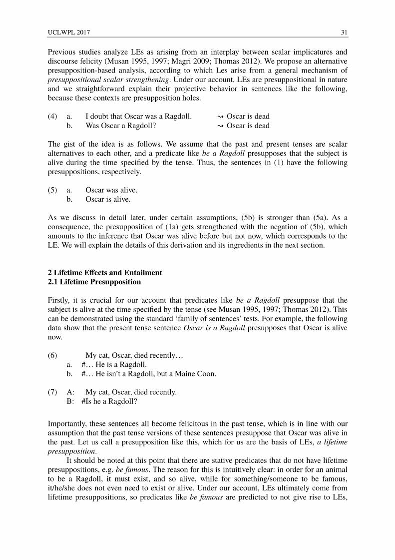
UCLWPL 2017 31

Previous studies analyze LEs as arising from an interplay between scalar implicatures and discourse felicity (Musan 1995, 1997; Magri 2009; Thomas 2012). We propose an alternative presupposition-based analysis, according to which Les arise from a general mechanism of presuppositional scalar strengthening. Under our account, LEs are presuppositional in nature and we straightforward explain their projective behavior in sentences like the following, because these contexts are presupposition holes.

(4) a. I doubt that Oscar was a Ragdoll. ↝ Oscar is dead b. Was Oscar a Ragdoll? ↝ Oscar is dead

The gist of the idea is as follows. We assume that the past and present tenses are scalar alternatives to each other, and a predicate like be a Ragdoll presupposes that the subject is alive during the time specified by the tense. Thus, the sentences in (1) have the following presuppositions, respectively.

(5) a. Oscar was alive. b. Oscar is alive.

As we discuss in detail later, under certain assumptions, (5b) is stronger than (5a). As a consequence, the presupposition of (1a) gets strengthened with the negation of (5b), which amounts to the inference that Oscar was alive before but not now, which corresponds to the LE. We will explain the details of this derivation and its ingredients in the next section.

2 Lifetime Effects and Entailment 2.1 Lifetime Presupposition Firstly, it is crucial for our account that predicates like be a Ragdoll presuppose that the subject is alive at the time specified by the tense (see Musan 1995, 1997; Thomas 2012). This can be demonstrated using the standard ‘family of sentences’ tests. For example, the following data show that the present tense sentence Oscar is a Ragdoll presupposes that Oscar is alive now. (6) My cat, Oscar, died recently… a. # … He is a Ragdoll. b. # … He isn’t a Ragdoll, but a Maine Coon. (7) A: My cat, Oscar, died recently. B: # Is he a Ragdoll?

Importantly, these sentences all become felicitous in the past tense, which is in line with our assumption that the past tense versions of these sentences presuppose that Oscar was alive in the past. Let us call a presupposition like this, which for us are the basis of LEs, a lifetime presupposition. It should be noted at this point that there are stative predicates that do not have lifetime presuppositions, e.g. be famous. The reason for this is intuitively clear: in order for an animal to be a Ragdoll, it must exist, and so alive, while for something/someone to be famous, it/he/she does not even need to exist or alive. Under our account, LEs ultimately come from lifetime presuppositions, so predicates like be famous are predicted to not give rise to LEs,

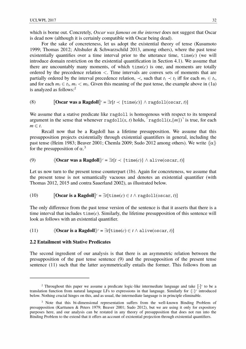
UCLWPL 2017 32

which is borne out. Concretely, Oscar was famous on the internet does not suggest that Oscar is dead now (although it is certainly compatible with Oscar being dead). For the sake of concreteness, let us adopt the existential theory of tense (Kusumoto 1999; Thomas 2012; Altshuler & Schwarzschild 2013, among others), where the past tense existentially quantifies over a time interval prior to the utterance time, time(c) (we will introduce domain restriction on the existential quantification in Section 4.1). We assume that there are uncountably many moments, of which time(c) is one, and moments are totally ordered by the precedence relation <. Time intervals are convex sets of moments that are partially ordered by the interval precedence relation, ≺, such that t1 ≺ t2 iff for each m1 ∈ t1, and for each m2 ∈ t2, m1 < m2. Given this meaning of the past tense, the example above in (1a) is analyzed as follows:2

(8) ⟦Oscar was a Ragdoll⟧c = ∃t [t ≺ {time(c)} ∧ ragdoll(oscar, t)]

We assume that a stative predicate like ragdoll is homogenous with respect to its temporal argument in the sense that whenever ragdoll(x, t) holds, ⌜ragdoll(x,{m})⌝ is true, for each m ∈ t. Recall now that be a Ragdoll has a lifetime presupposition. We assume that this presupposition projects existentially through existential quantifiers in general, including the past tense (Heim 1983; Beaver 2001; Chemla 2009; Sudo 2012 among others). We write ⟪⟫ for the presupposition of .3

(9) ⟪Oscar was a Ragdoll⟫c = ∃t [t ≺ {time(c)} ∧ alive(oscar, t)]

Let us now turn to the present tense counterpart (1b). Again for concreteness, we assume that the present tense is not semantically vacuous and denotes an existential quantifier (with Thomas 2012, 2015 and contra Sauerland 2002), as illustrated below.

(10) ⟦Oscar is a Ragdoll⟧c = ∃t [time(c) ∈ t ∧ ragdoll(oscar, t)]

The only difference from the past tense version of the sentence is that it asserts that there is a time interval that includes time(c). Similarly, the lifetime presupposition of this sentence will look as follows with an existential quantifier.

(11) ⟪Oscar is a Ragdoll⟫c = ∃t [time(c) ∈ t ∧ alive(oscar, t)] 2.2 Entailment with Stative Predicates The second ingredient of our analysis is that there is an asymmetric relation between the presupposition of the past tense sentence (9) and the presupposition of the present tense sentence (11) such that the latter asymmetrically entails the former. This follows from an

2 Throughout this paper we assume a predicate logic-like intermediate language and take ⟦·⟧c to be a translation function from natural language LFs to expressions in that language. Similarly for ⟪·⟫c introduced below. Nothing crucial hinges on this, and as usual, the intermediate language is in principle eliminable.

3 Note that this bi-dimensional representation suffers from the well-known Binding Problem of presupposition (Karttunen & Peters 1979; Beaver 2001; Sudo 2012), but we are using it only for expository purposes here, and our analysis can be restated in any theory of presupposition that does not run into the Binding Problem to the extend that it offers an account of existential projection through existential quantifiers.

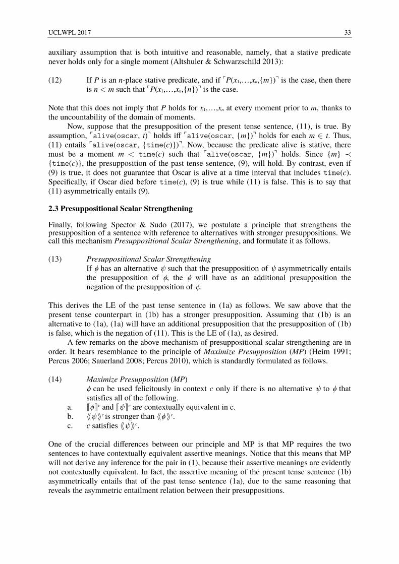
UCLWPL 2017 33

auxiliary assumption that is both intuitive and reasonable, namely, that a stative predicate never holds only for a single moment (Altshuler & Schwarzschild 2013):

(12) If P is an n-place stative predicate, and if ⌜P(x1,…,xn,{m})⌝ is the case, then there is n < m such that ⌜P(x1,…,xn,{n})⌝ is the case.

Note that this does not imply that P holds for x1,…,xn at every moment prior to m, thanks to the uncountability of the domain of moments. Now, suppose that the presupposition of the present tense sentence, (11), is true. By assumption, ⌜alive(oscar, t)⌝ holds iff ⌜alive(oscar, {m})⌝ holds for each m ∈ t. Thus, (11) entails ⌜alive(oscar, {time(c)})⌝. Now, because the predicate alive is stative, there must be a moment m < time(c) such that ⌜alive(oscar, {m})⌝ holds. Since {m} ≺

{time(c)}, the presupposition of the past tense sentence, (9), will hold. By contrast, even if (9) is true, it does not guarantee that Oscar is alive at a time interval that includes time(c). Specifically, if Oscar died before time(c), (9) is true while (11) is false. This is to say that (11) asymmetrically entails (9). 2.3 Presuppositional Scalar Strengthening Finally, following Spector & Sudo (2017), we postulate a principle that strengthens the presupposition of a sentence with reference to alternatives with stronger presuppositions. We call this mechanism Presuppositional Scalar Strengthening, and formulate it as follows. (13) Presuppositional Scalar Strengthening

If ϕ has an alternative ψ such that the presupposition of ψ asymmetrically entails the presupposition of ϕ, the ϕ will have as an additional presupposition the negation of the presupposition of ψ.

This derives the LE of the past tense sentence in (1a) as follows. We saw above that the present tense counterpart in (1b) has a stronger presupposition. Assuming that (1b) is an alternative to (1a), (1a) will have an additional presupposition that the presupposition of (1b) is false, which is the negation of (11). This is the LE of (1a), as desired. A few remarks on the above mechanism of presuppositional scalar strengthening are in order. It bears resemblance to the principle of Maximize Presupposition (MP) (Heim 1991; Percus 2006; Sauerland 2008; Percus 2010), which is standardly formulated as follows.

(14) Maximize Presupposition (MP)

ϕ can be used felicitously in context c only if there is no alternative ψ to ϕ that satisfies all of the following.

a. ⟦ϕ ⟧c and ⟦ψ ⟧c are contextually equivalent in c. b. ⟪ψ ⟫c

is stronger than ⟪ϕ ⟫c. c. c satisfies ⟪ψ ⟫c. One of the crucial differences between our principle and MP is that MP requires the two sentences to have contextually equivalent assertive meanings. Notice that this means that MP will not derive any inference for the pair in (1), because their assertive meanings are evidently not contextually equivalent. In fact, the assertive meaning of the present tense sentence (1b) asymmetrically entails that of the past tense sentence (1a), due to the same reasoning that reveals the asymmetric entailment relation between their presuppositions.

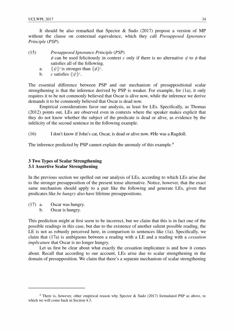
UCLWPL 2017 34

It should be also remarked that Spector & Sudo (2017) propose a version of MP without the clause on contextual equivalence, which they call Presupposed Ignorance Principle (PSP).

(15) Presupposed Ignorance Principle (PSP)

ϕ can be used felicitously in context c only if there is no alternative ψ to ϕ that satisfies all of the following.

a. ⟪ψ ⟫c is stronger than ⟪ϕ ⟫c.

b. c satisfies ⟪ψ ⟫c. The essential difference between PSP and our mechanism of presuppositional scalar strengthening is that the inference derived by PSP is weaker. For example, for (1a), it only requires it to be not commonly believed that Oscar is alive now, while the inference we derive demands it to be commonly believed that Oscar is dead now. Empirical considerations favor our analysis, as least for LEs. Specifically, as Thomas (2012) points out, LEs are observed even in contexts where the speaker makes explicit that they do not know whether the subject of the predicate is dead or alive, as evidence by the infelicity of the second sentence in the following example. (16) I don’t know if John’s cat, Oscar, is dead or alive now. # He was a Ragdoll. The inference predicted by PSP cannot explain the anomaly of this example.4

3 Two Types of Scalar Strengthening 3.1 Assertive Scalar Strengthening In the previous section we spelled out our analysis of LEs, according to which LEs arise due to the stronger presupposition of the present tense alternative. Notice, however, that the exact same mechanism should apply to a pair like the following and generate LEs, given that predicates like be hungry also have lifetime presuppositions. (17) a. Oscar was hungry. b. Oscar is hungry. This prediction might at first seem to be incorrect, but we claim that this is in fact one of the possible readings in this case, but due to the existence of another salient possible reading, the LE is not as robustly perceived here, in comparison to sentences like (1a). Specifically, we claim that (17a) is ambiguous between a reading with a LE and a reading with a cessation implicature that Oscar is no longer hungry. Let us first be clear about what exactly the cessation implicature is and how it comes about. Recall that according to our account, LEs arise due to scalar strengthening in the domain of presupposition. We claim that there’s a separate mechanism of scalar strengthening

4 There is, however, other empirical reason why Spector & Sudo (2017) formulated PSP as above, to which we will come back in Section 4.3.

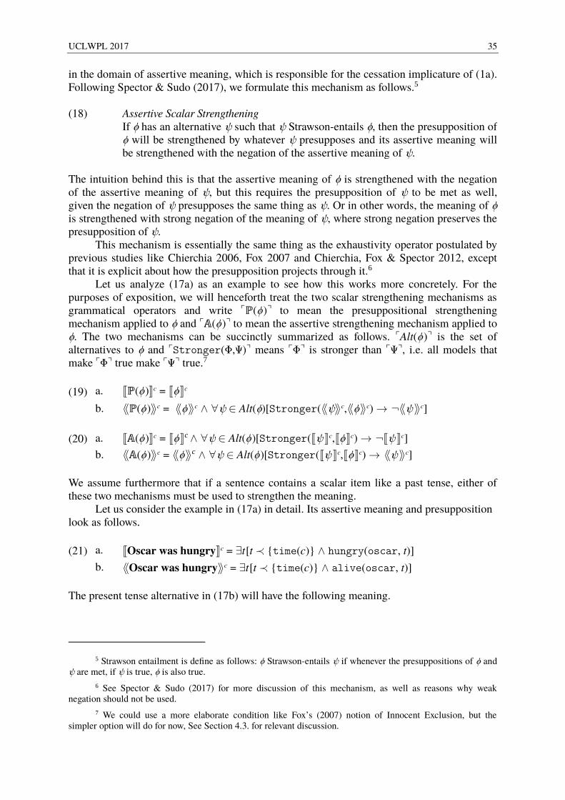
UCLWPL 2017 35

in the domain of assertive meaning, which is responsible for the cessation implicature of (1a). Following Spector & Sudo (2017), we formulate this mechanism as follows.5 (18) Assertive Scalar Strengthening

If ϕ has an alternative ψ such that ψ Strawson-entails ϕ, then the presupposition of ϕ will be strengthened by whatever ψ presupposes and its assertive meaning will be strengthened with the negation of the assertive meaning of ψ.

The intuition behind this is that the assertive meaning of ϕ is strengthened with the negation of the assertive meaning of ψ, but this requires the presupposition of ψ to be met as well, given the negation of ψ presupposes the same thing as ψ. Or in other words, the meaning of ϕ is strengthened with strong negation of the meaning of ψ, where strong negation preserves the presupposition of ψ. This mechanism is essentially the same thing as the exhaustivity operator postulated by previous studies like Chierchia 2006, Fox 2007 and Chierchia, Fox & Spector 2012, except that it is explicit about how the presupposition projects through it.6 Let us analyze (17a) as an example to see how this works more concretely. For the purposes of exposition, we will henceforth treat the two scalar strengthening mechanisms as grammatical operators and write ⌜ℙ(ϕ)⌝ to mean the presuppositional strengthening mechanism applied to ϕ and ⌜𝔸(ϕ)⌝ to mean the assertive strengthening mechanism applied to ϕ. The two mechanisms can be succinctly summarized as follows. ⌜Alt(ϕ)⌝ is the set of alternatives to ϕ and ⌜Stronger(Φ,Ψ)⌝ means ⌜Φ⌝ is stronger than ⌜Ψ⌝, i.e. all models that make ⌜Φ⌝ true make ⌜Ψ⌝ true.7

(19) a. ⟦ℙ(ϕ)⟧c = ⟦ϕ⟧c

b. ⟪ℙ(ϕ)⟫c = ⟪ϕ⟫c ∧ ∀ψ ∈ Alt(ϕ)[Stronger(⟪ψ⟫c,⟪ϕ⟫c) → ¬⟪ψ ⟫c]

(20) a. ⟦𝔸(ϕ)⟧c = ⟦ϕ⟧c ∧ ∀ψ ∈ Alt(ϕ)[Stronger(⟦ψ ⟧c,⟦ϕ⟧c) → ¬⟦ψ ⟧c]

b. ⟪𝔸(ϕ)⟫c = ⟪ϕ⟫c ∧ ∀ψ ∈ Alt(ϕ)[Stronger(⟦ψ ⟧c,⟦ϕ⟧c) → ⟪ψ ⟫c]

We assume furthermore that if a sentence contains a scalar item like a past tense, either of these two mechanisms must be used to strengthen the meaning. Let us consider the example in (17a) in detail. Its assertive meaning and presupposition look as follows.

(21) a. ⟦Oscar was hungry⟧c = ∃t [t ≺ {time(c)} ∧ hungry(oscar, t)]

b. ⟪Oscar was hungry⟫c = ∃t [t ≺ {time(c)} ∧ alive(oscar, t)]

The present tense alternative in (17b) will have the following meaning.

5 Strawson entailment is define as follows: ϕ Strawson-entails ψ if whenever the presuppositions of ϕ and ψ are met, if ψ is true, ϕ is also true.

6 See Spector & Sudo (2017) for more discussion of this mechanism, as well as reasons why weak negation should not be used.

7 We could use a more elaborate condition like Fox’s (2007) notion of Innocent Exclusion, but the simpler option will do for now, See Section 4.3. for relevant discussion.

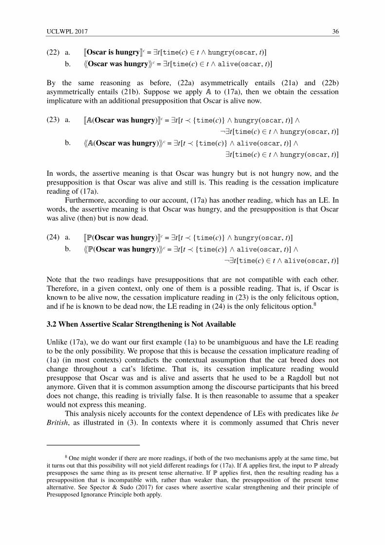
UCLWPL 2017 36

(22) a. ⟦Oscar is hungry⟧c = ∃t [time(c) ∈ t ∧ hungry(oscar, t)]

b. ⟪Oscar was hungry⟫c = ∃t [time(c) ∈ t ∧ alive(oscar, t)]

By the same reasoning as before, (22a) asymmetrically entails (21a) and (22b) asymmetrically entails (21b). Suppose we apply 𝔸 to (17a), then we obtain the cessation implicature with an additional presupposition that Oscar is alive now.

(23) a. ⟦𝔸(Oscar was hungry)⟧c = ∃t [t ≺ {time(c)} ∧ hungry(oscar, t)] ∧

¬∃t [time(c) ∈ t ∧ hungry(oscar, t)]

b. ⟪𝔸(Oscar was hungry)⟫c = ∃t [t ≺ {time(c)} ∧ alive(oscar, t)] ∧

∃t [time(c) ∈ t ∧ hungry(oscar, t)]

In words, the assertive meaning is that Oscar was hungry but is not hungry now, and the presupposition is that Oscar was alive and still is. This reading is the cessation implicature reading of (17a). Furthermore, according to our account, (17a) has another reading, which has an LE. In words, the assertive meaning is that Oscar was hungry, and the presupposition is that Oscar was alive (then) but is now dead.

(24) a. ⟦ℙ(Oscar was hungry)⟧c = ∃t [t ≺ {time(c)} ∧ hungry(oscar, t)]

b. ⟪ℙ(Oscar was hungry)⟫c = ∃t [t ≺ {time(c)} ∧ alive(oscar, t)] ∧

¬∃t [time(c) ∈ t ∧ alive(oscar, t)]

Note that the two readings have presuppositions that are not compatible with each other. Therefore, in a given context, only one of them is a possible reading. That is, if Oscar is known to be alive now, the cessation implicature reading in (23) is the only felicitous option, and if he is known to be dead now, the LE reading in (24) is the only felicitous option.8 3.2 When Assertive Scalar Strengthening is Not Available Unlike (17a), we do want our first example (1a) to be unambiguous and have the LE reading to be the only possibility. We propose that this is because the cessation implicature reading of (1a) (in most contexts) contradicts the contextual assumption that the cat breed does not change throughout a cat’s lifetime. That is, its cessation implicature reading would presuppose that Oscar was and is alive and asserts that he used to be a Ragdoll but not anymore. Given that it is common assumption among the discourse participants that his breed does not change, this reading is trivially false. It is then reasonable to assume that a speaker would not express this meaning. This analysis nicely accounts for the context dependence of LEs with predicates like be British, as illustrated in (3). In contexts where it is commonly assumed that Chris never

8 One might wonder if there are more readings, if both of the two mechanisms apply at the same time, but it turns out that this possibility will not yield different readings for (17a). If 𝔸 applies first, the input to ℙ already presupposes the same thing as its present tense alternative. If ℙ applies first, then the resulting reading has a presupposition that is incompatible with, rather than weaker than, the presupposition of the present tense alternative. See Spector & Sudo (2017) for cases where assertive scalar strengthening and their principle of Presupposed Ignorance Principle both apply.

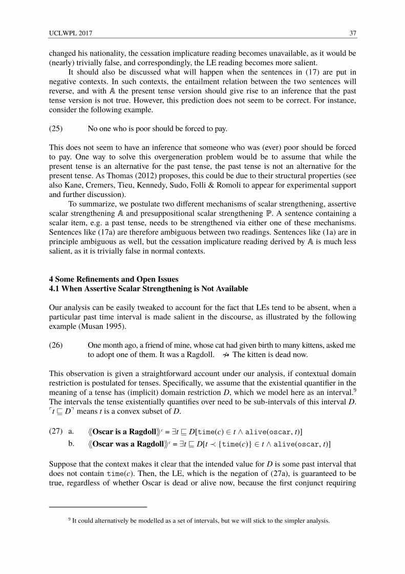
UCLWPL 2017 37

changed his nationality, the cessation implicature reading becomes unavailable, as it would be (nearly) trivially false, and correspondingly, the LE reading becomes more salient. It should also be discussed what will happen when the sentences in (17) are put in negative contexts. In such contexts, the entailment relation between the two sentences will reverse, and with 𝔸 the present tense version should give rise to an inference that the past tense version is not true. However, this prediction does not seem to be correct. For instance, consider the following example. (25) No one who is poor should be forced to pay. This does not seem to have an inference that someone who was (ever) poor should be forced to pay. One way to solve this overgeneration problem would be to assume that while the present tense is an alternative for the past tense, the past tense is not an alternative for the present tense. As Thomas (2012) proposes, this could be due to their structural properties (see also Kane, Cremers, Tieu, Kennedy, Sudo, Folli & Romoli to appear for experimental support and further discussion). To summarize, we postulate two different mechanisms of scalar strengthening, assertive scalar strengthening 𝔸 and presuppositional scalar strengthening ℙ. A sentence containing a scalar item, e.g. a past tense, needs to be strengthened via either one of these mechanisms. Sentences like (17a) are therefore ambiguous between two readings. Sentences like (1a) are in principle ambiguous as well, but the cessation implicature reading derived by 𝔸 is much less salient, as it is trivially false in normal contexts.

4 Some Refinements and Open Issues 4.1 When Assertive Scalar Strengthening is Not Available Our analysis can be easily tweaked to account for the fact that LEs tend to be absent, when a particular past time interval is made salient in the discourse, as illustrated by the following example (Musan 1995). (26) One month ago, a friend of mine, whose cat had given birth to many kittens, asked me to adopt one of them. It was a Ragdoll. ⇝/ The kitten is dead now.

This observation is given a straightforward account under our analysis, if contextual domain restriction is postulated for tenses. Specifically, we assume that the existential quantifier in the meaning of a tense has (implicit) domain restriction D, which we model here as an interval.9 The intervals the tense existentially quantifies over need to be sub-intervals of this interval D. ⌜t ⊑ D⌝ means t is a convex subset of D.

(27) a. ⟪Oscar is a Ragdoll⟫c = ∃t ⊑ D[time(c) ∈ t ∧ alive(oscar, t)]

b. ⟪Oscar was a Ragdoll⟫c = ∃t ⊑ D[t ≺ {time(c)} ∈ t ∧ alive(oscar, t)]

Suppose that the context makes it clear that the intended value for D is some past interval that does not contain time(c). Then, the LE, which is the negation of (27a), is guaranteed to be true, regardless of whether Oscar is dead or alive now, because the first conjunct requiring

9 It could alternatively be modelled as a set of intervals, but we will stick to the simpler analysis.

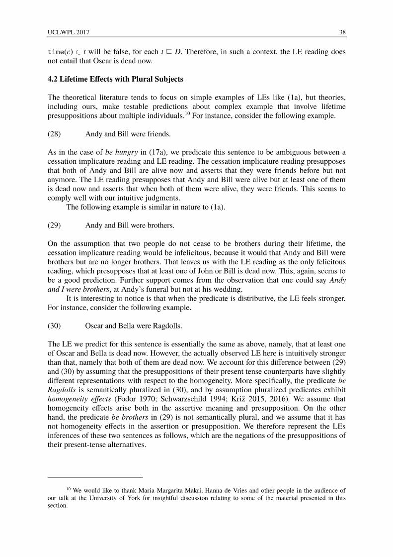
UCLWPL 2017 38

time(c) ∈ t will be false, for each t ⊑ D. Therefore, in such a context, the LE reading does not entail that Oscar is dead now. 4.2 Lifetime Effects with Plural Subjects The theoretical literature tends to focus on simple examples of LEs like (1a), but theories, including ours, make testable predictions about complex example that involve lifetime presuppositions about multiple individuals.10 For instance, consider the following example. (28) Andy and Bill were friends. As in the case of be hungry in (17a), we predicate this sentence to be ambiguous between a cessation implicature reading and LE reading. The cessation implicature reading presupposes that both of Andy and Bill are alive now and asserts that they were friends before but not anymore. The LE reading presupposes that Andy and Bill were alive but at least one of them is dead now and asserts that when both of them were alive, they were friends. This seems to comply well with our intuitive judgments. The following example is similar in nature to (1a). (29) Andy and Bill were brothers. On the assumption that two people do not cease to be brothers during their lifetime, the cessation implicature reading would be infelicitous, because it would that Andy and Bill were brothers but are no longer brothers. That leaves us with the LE reading as the only felicitous reading, which presupposes that at least one of John or Bill is dead now. This, again, seems to be a good prediction. Further support comes from the observation that one could say Andy and I were brothers, at Andy’s funeral but not at his wedding. It is interesting to notice is that when the predicate is distributive, the LE feels stronger. For instance, consider the following example. (30) Oscar and Bella were Ragdolls. The LE we predict for this sentence is essentially the same as above, namely, that at least one of Oscar and Bella is dead now. However, the actually observed LE here is intuitively stronger than that, namely that both of them are dead now. We account for this difference between (29) and (30) by assuming that the presuppositions of their present tense counterparts have slightly different representations with respect to the homogeneity. More specifically, the predicate be Ragdolls is semantically pluralized in (30), and by assumption pluralized predicates exhibit homogeneity effects (Fodor 1970; Schwarzschild 1994; Križ 2015, 2016). We assume that homogeneity effects arise both in the assertive meaning and presupposition. On the other hand, the predicate be brothers in (29) is not semantically plural, and we assume that it has not homogeneity effects in the assertion or presupposition. We therefore represent the LEs inferences of these two sentences as follows, which are the negations of the presuppositions of their present-tense alternatives.

10 We would like to thank Maria-Margarita Makri, Hanna de Vries and other people in the audience of our talk at the University of York for insightful discussion relating to some of the material presented in this section.

UCLWPL 2017 39

(31) a. ¬∃t [time(c) ∈ t ∧ alive(andy, t) ∧ alive(bill, t)]

b. ¬∃t [time(c) ∈ t ∧ *alive(andy ⊕ bill, t)]

Crucially, the pluralization operator * introduces homogeneity and the latter, but not the former, entails that both of Andy and Bill are dead now. 4.3 Presupposed Ignorance As mentioned in Section 2.3, our mechanism of presupposed scalar strengthening derives a stronger inference than Spector & Sudo’s (2017) Presupposed Ignorance Principle (PSP). They formulate it as such to account for the following type of sentence. (32) Andy lives in Aberdeen. # Bill lives in Aberdeen or Brighton, too. They crucially assume that the alternatives for the second sentence here include the following two (Sauerland 2004). (33) a. Bill lives in Aberdeen, too. b. Bill lives in Brighton, too. Assuming that too is anaphoric to Andy, these presuppose that Andy lives in Aberdeen and that Andy lives in Brighton, respectively. These presuppositions are stronger than the presuppositions of the disjunctive sentence above, so PSP requires them to be not satisfied. In the example above, when the second sentence is uttered, it is already known that Andy lives in Aberdeen. Therefore, the inference derived by PSP is not satisfied, which accounts for the infelicity. Our account, as it stands now, predicts contradictory presuppositions with the same alternatives. That is, it negates the presuppositions of both of these alternatives, which is to say that Andy does not live in Aberdeen and Andy does not live in Brighton. This inference is too strong, because the following example is felicitous. (34) Andy lives in Aberdeen or Brighton. Bill lives in Aberdeen or Brighton, too. We could adopt a more stringent condition on which alternatives to negate (cf. innocently excludable alternatives in the sense of Fox 2007), but that would not predict any inference for the disjunctive sentence in question, failing to account for the infelicity of (32). However, recall that the example in (16) indicates that the ignorance inference that PSP generates is not strong enough for LEs. (16) I don’t know if John’s cat, Oscar, is dead or alive now. # He was a Ragdoll. Generally, weaker inferences like the one we observe for (32) are only observed with scalar items that trigger ignorance inferences like disjunction, at least, etc. We haven’t found, at the moment, a way to reconcile the facts exemplified by (16) and (32), but we would like to note that a similar tension arises in the domain of assertive scalar strengthening. Concretely, one normally gets a strong scalar inference (so-called secondary scalar implicature by Sauerland 2004) for sentences like (35a) and (35b), in comparison to the ignorance inference of sentences like (35c).

UCLWPL 2017 40

(35) a. Most of my students speak Mandarin Chinese. ↝ Not all of them do.

b. It is chilly in Chicago. ↝ It is not terribly cold in Chicago. Daniel is in Denver of Detroit.

Fox (2007), for example, claims that the stronger inferences of the first two examples above are due to a grammatical operator, while the ignorance inference of the kind exhibited by (35c) is due to Gicean reasoning. If this is on the right track, it is perhaps not entirely inconceivable that a similar division of labor between semantics and pragmatics is observed in the domain of presuppositions. We will have to leave this issue open here. 5 Comparison with Previous Accounts Lastly we would like to briefly compare our account of LEs with representative precedents. Musan (1995, 1997) assumes that LEs are essentially the same inference as cessation implicatures. That is, (1a), for example, has a cessation implicature that Oscar is no longer a Ragdoll, and given that a cat does not change its breed throughout its lifetime, so her reasoning goes, this implies that Oscar is dead. As Thomas (2012) discusses in detail, certain aspects of her analysis are unclear, especially regarding how presuppositions ought to project. However, even putting these issues aside, it makes a problematic prediction with respect to the projection of LEs. When (1a) is put in a scalar implicature cancelling context, it is predicted that LEs cease to arise. As we saw in (4), this prediction is not borne out. On the other hand, this is exactly what our presuppositional account predicts, because according to our account, the presuppositions of the past tense and present tense sentences are compared, and being presuppositions, they are expect to project out in contexts like above. Consequently, LEs are predicted just as in the simple example in (1a). Magri (2009, 2011) derives LEs by an interplay between cessation implicatures and contextually determine alternatives. Unlike Musan, Magri assumes that the cessation implicature of (1a) is infelicitous. He then proposes that (1a) is felicitous in contexts where the cessation implicature is blocked. Specifically, he argues that in contexts where it is known that Oscar is alive, the past tense sentence (1a) and its present tense alternative (1b) are contextually equivalent, and in such contexts, the cessation implicature obligatorily arises. On the other hand, in contexts where the two sentences are not contextually equivalent, the cessation implicature can be blocked. He argues that these contexts are exactly the contexts where Oscar is not known to be alive. However, one shortcoming of this account is, as Thomas (2012) points out, that it predicts LEs to be blocked in an ignorance context like (16), because the two sentences are not contextually equivalent in such a context. Recall that we have a straightforward account of (16) as for us the LE of this example is a bona fide presupposition. In addition, the observations made in Section 4.2 appear also problematic for Magri’s account. Recall that we account for the difference between collective and distributive predicates by assuming that the latter give rise to homogeneity effects with respect to plural subjects, which results in a stronger inference. Since LEs do not involve negation of the present tense alternative under Magri’s account, it is unclear to us how the contrast could be explained. 6 Conclusion When used in combination with past tense, most stative predicates (e.g. be a Ragdoll) tend to give rise to a Lifetime Effect inference that the subject is dead. Previous studies analyzed

UCLWPL 2017 41

these effects as arising from the interaction between scalar implicatures and discourse felicity. In this paper, we have proposed an alternative presuppositional analysis based on recent work by Spector & Sudo (2017). The resulting system is one in which cessation implicatures and lifetime effects arise in parallel as a result of an implicature strengthening mechanism applying at different levels: at the assertion level for cessation implicatures and at the presuppositional level for lifetime effects inferences. As we discussed, the presuppositional approach proposed here makes better predictions than the scalar implicature one, in particular with respect to the projection behaviour of LEs, ignorance inference contexts and the interaction between plurality and LEs.

References Altshuler, D., & Roger Schwarzschild, R, (2013) Correlating cessation with double access. In Proceedings of the

19th Amseterdam Colloquium. Beaver, D. (2001). Presupposition and Assertion in Dynamic Semantics. Stanford: CSLI. Chemla, E. (2009). Presuppositions of quantified sentences: experimental data. Natural Language Semantics,

17(4), 299–340. Chierchia, Gennaro. 2006. Broaden your views: Implicatures of domain widening and the “Logicality” of

language. Linguistic Inquiry, 37(4), 535–590. Chierchia, G., Fox, D., & Spector. B. (2012). Scalar implicature as a grammatical phenomenon. In C.

Maienborn, K. von Heusinger & P. Portner (eds.), Semantics: An International Handbook of Natural Language Meaning, 2297–2331. Berlin: de Gruyter.

Fodor, J. (1970). The Linguistic Description of Opaque Contexts. Doctoral dissertation. MIT. Fox, D. (2007). Free choice and the theory of scalar implicatures. In U. Sauerland & P. Stateva (eds.),

Presupposition and Implicature in Compositional Semantics, 71–112. Palgrave Macmillan. Heim, I. (1983). On the projection problem for presuppositions. In WCCFL 2, 114–125. Heim, I. (1991). Artikel und Definitheit. In A. von Stechow & D. Wunderlich (eds.), Semantik: Ein

internationales Handbuch der zeitgenössischen Forschung/Semantics: An International Handbook of Contemporary Research, 487–535. Berlin: de Gruyter.

Kane, F., Cremers, A., Tieu, L., Kennedy, L., Sudo, Y., Folli, R, & Romoli, J. (to appear). Testing theories of temporal inferences: Evidence from child language. In Proceedings of Sinn und Bedeutung 22.

Karttunen, L., & Peters, S. (1979). Conventional implicature. In C-K.Oh & D. Dinneen (eds.), Syntax and Semantics 11: Presupposition, 1–56. New York: Academic Press.

Križ, M. (2015). Aspects of Homogeneity in the Semantics of Natural Language. Doctoral dissertation. University of Vienna.

Križ, M. (2016). Homogeneity, non-maximality, and all. Journal of Semantics 33(3). 493–539. Kusumoto, K. (1999). Tense in Embedded Context. Doctoral dissertation. University of Massachusetts, Amherst. Magri, G. (2009). A theory of individual-level predicates based on blind mandatory scalar implicatures. Natural

Language Semantics, 17(3), 245–297. Magri, G. (2011). Another argument for embedded scalar implicatures based on oddness in downward entailing

environments. Semantics & Pragmatics, 4(6), 1–51. Musan, R. (1995). On the Temporal Interpretation of Noun Phrases. Doctoral dissertation. MIT. Musan, R. (1997). Tense, predicates, and lifetime effects. Natural Language Semantics, 5, 271–301. Percus, O. (2006). Antipresuppositions. Tech. rep. Japan Society for the Promotion of Science. Report of the

Grant-in-Aid for Scientific Research (B), Project No. 15320052. Percus, O. (2010). Antipresuppositions revisited. Talk given at CRISCO, Université de Caen. Sauerland, U. (2002). The present tense is vacuous. Snippets, 6, 12–13. Sauerland, U. (2004). Scalar implicatures in complex sentences. Linguistics and Philosophy 27(3), 367–391. Sauerland, U. (2008). Implicated presuppositions. In A. Steube (ed.), The Discourse Potential of Underspecified

Structures Language, Context and Cognition, 581–600. Berlin: Mouton de Gruyter. Schwarzschild, R. (1994). Plurals, presuppositions and the sources of distributivity. Natural Language

Semantics, 2(3), 201–248. Spector, B., & Sudo, Y. (2017). Presupposed ignorance and exhaustification: how scalar implicatures and

presuppositions interact. Linguistics and Philosophy, 40(5), 473-517. Sudo, Y. (2012). On the Semantics of Phi Features on Pronouns. Doctoral dissertation. MIT. Thomas, G. (2012). Temporal Implicatures. Doctoral dissertation. MIT. Thomas, G. (2015). The present tense is not vacuous. Journal of Semantics, 32(4), 685–747.

Doxastic Diversity and Covert Temporal Operators*

Gregor Williamson

Abstract The purpose of this paper is relatively modest. Firstly, I propose that the presuppositions of certain attitude predicates such as expect, hope and want can predictably constrain the temporal orientation of their infinitival complements. Secondly, I attempt to defend the position that future oriented infinitivals feature a covert temporal operator. Keywords: Infinitival Tense, doxastic diversity presuppositions, de se, ordering predicates, covert temporal operators

1 Introduction Propositional attitude verbs which select infinitival complements are often divided into two classes. Those which give rise to a future oriented reading, and those which give rise to a simultaneous reading. (1) a. John {wanted/hoped/expected Mary} to be at the party. future oriented b. John {claimed/believed Mary} to be at the party. simultaneous While the infinitival complements in (1) have different temporal interpretations, on the surface they appear identical. There are two schools of thought concerning how to handle this disparity between interpretation on the one hand, and the surface form on the other. The first group of proposals I will refer to as syntactic accounts. These accounts assume that, while these complements look identical, there is in fact covert material present in the future oriented complement which is absent in the simultaneous complement. Early proponents of this account treat this extra material as a form of covert irrealis Tense (Stowell, 1982; Martin, 2001 inter alia), while more recent accounts propose a covert future operator (Abusch, 2004; Wurmbrand, 2014; Grano, 2015). In order to prevent overgeneration of future oriented infinitives, syntactic accounts often make an appeal (either explicit or implicit) to the lexical semantics of the selecting verb in order to limit the distribution, or interpretation, of the covert future operator (Stowell, 1982; Landau, 2000; Abusch, 2004; Wurmbrand, 2014; Grano, 2015). However, they rarely attempt to provide an explicit semantics which can derive this distribution. In contrast, accounts which I will call semantic accounts maintain that the infinitival complements in (1) do not differ in structure or meaning. Rather, it is the lexical semantics of the selecting verb which determine the temporality of the embedded infinitival. These accounts build the posteriority of the future orientated infinitivals in (1a) directly into the selecting verb itself (Katz, 2001; Pearson, 2016, 2017). In this paper, I will suggest that a syntactic account is to be preferred. But we must rely on the lexical semantics of the selecting verb in order to correctly predict the distribution of

*Thanks to Hans van de Koot, Yasutada Sudo, Hazel Pearson and Nathan Klinedinst for helpful discussion on the ideas in this paper. Thanks also to the UCL Syntax Reading Group, where some of the ideas found in this paper were presented on 17th October 2017. Funding for this work was provided by the London Arts and Humanities Partnership. All errors are my own.

UCLWPL 2017 43

the covert future operator. In section 2, I will address instances in which the future oriented predicates in (1a) can have complements which have a simultaneous reading. I argue that the distribution of simultaneous complements is restricted in a principled manner by the lexical semantics of the verb. I show that expect can license simultaneous reading with an ECM complement, as well as certain control complements provided its doxastic uncertainty requirement is satisfied (Anand & Hacquard, 2013). The verb hope receives a similar treatment to expect. Conversely, want is argued to lack such a requirement, and as such, it can license simultaneous readings more generally. In section 3 of this paper, I will offer some reasons to think a syntactic account which posits a covert temporal operator in future oriented infinitives is preferable to a semantic account. In addition, problems will be noted for two specific semantic accounts (Katz, 2001; Pearson, 2016). Finally, some of the seemingly less attractive aspects of a syntactic account will be shown to be tolerable given some reasonable assumptions. 2 Doxastic Diversity and Temporal Orientation It has been observed by Abusch (2004) that certain predicates can license future oriented and simultaneous infinitival complements, while others cannot. Among those which can is the verb expect.1 Pesetsky (1992) notes that ECM complements to expect can receive a simultaneous reading akin to believe provided the complement concerns something “unknown to the speaker” (p.29). I will suggest that this requirement takes the form of a doxastic uncertainty requirement (Anand & Hacquard, 2013), a diversity condition on the Modal Base of predicates which rank doxastic alternatives according to an Ordering Source (Kratzer, 1977, 1981, 2012; von Fintel, 1999). This observation for expect will be shown to extend to the emotive doxastic hope which has also been argued to have such a requirement. Finally, it will be shown that the non-doxastic want is not subject to the same requirement and is thus more flexible in its possible temporal orientation. 2.1 Expect

Pesetsky (1992) observed that ECM complements to expect can receive a simultaneous belief-type reading.2 (2) I expect there to be flowers on the table. Pesetsky also noted that such a sentence is inappropriate if the attitude holder knows that there are flowers on the table. He proposes that expect expresses a belief about something unknown to the attitude holder. While this characterization is intuitive, we will instead pursue the proposal that expect expresses that the attitude holder finds the prejacent likely but presupposes that the attitude holder is not certain with respect to the truth of the complement. Specifically, we adopt the proposal of von Fintel (1999) that, for certain predicates, worlds

1 Abusch discusses the verb predict (i) which can have either a future oriented or simultaneous reading. While I do not discuss this verb here, I believe it can be given more or less the same semantics as expect. I concentrate on expect because it can take part in both control and ECM constructions.

(i) Monique is predicted to be pregnant {already/by next week}.

2 Pesetsky’s main concern is comparing the propositional uses of expect discussed here with those that have a bouletic flavour (Bresnan, 1972). I will have nothing to say about those other uses here.

UCLWPL 2017 44

supplied by a Modal Base (MB) are ranked according to an Ordering Source (OS) (Kratzer, 1977, 1981, 2012). In what follows, I assume a centered worlds semantics wherein an attitude holder’s set of doxastic alternatives, for example, is not a set of worlds, but rather a set of world-time-individual triples, or centered worlds.3

(3) Doxx,t,w =

{

⟨w′, t′, y⟩ ||

it is compatible with whatx believes in w at t for :● w to be w′ ● t to be t′ in w′● x to be y in w′ at t′

}

To rank the doxastic alternatives of the attitude holder, we define an operator MaxOS which picks out the set of best worlds according to a partial ordering relation ≺OS.

(4) a. MaxOS(MB) = {⟨w, t, x⟩ ∈ MB : ¬∃⟨w′, t′, y⟩ ∈ MB : ⟨w′, t′, y⟩ ≺OS ⟨w, t, x⟩}

b. where ⟨w′, t′, y⟩ ≺OS ⟨w, t, x⟩ iff

{P ∈ OS : P(x)(t)(w)} ⊂ {P ∈ OS : P(y)(t′)(w′)}

Taken together, this machinery will give us a semantics such as the following for expect.4

(5) a. ⟦expect⟧ = λwλtλPλx. ∀⟨w′, t′, y⟩ ∈ MaxPROBx,t,w(Doxx,t,w) : P(y)(t′)(w′)

b. presupposes ∃⟨w″, t″, z⟩ ∈ Doxx,t,w : P(z)(t″)(w″) = 1

∧ ∃⟨w″, t″, z⟩ ∈ Doxx,t,w : P(z)(t″)(w″) = 0 c. where PROBx,t,w = {P⟨e,⟨i,st⟩⟩ : x finds it likely at t in w to have property P} This semantics universally quantifies over the most likely doxastic alternatives of the attitude holder, while presupposing that the doxastic modal base is diverse with respect to the truth of the complement. Since it is generally the case that an attitude holder can be uncertain about whether a given property holds of another individual at the attitude holder’s candidate for NOW, it is not surprising that ECM complements can have a simultaneous reading. Nor is it surprising that expect can have future oriented control complements, as it is typically the case that one can be uncertain with respect to whether a given property will hold of one’s SELF at some future time. (6) John expected to see a bunch of dead flowers on the table when returned home. What is decidedly less common is that one can be uncertain with respect to whether a property simultaneously holds of one’s SELF. This is the state of affairs which would have to

3 The motivation for centered worlds is well-documented and will not be rehearsed here (see e.g., Lewis, 1979; Chierchia, 1989; Abusch, 1998; Stephenson, 2007; Uegaki, 2011; Pearson, 2016 inter alia). The individual coordinate represents attitude holder’s candidates for his/her SELF. Pronouns which are coindexed with the individual coordinate, such as PRO, receive an interpretation de se (Chierchia, 1989). The time coordinate represents the attitude holder’s candidates for NOW, temporal pronouns coindexed with the time coordinate receive an interpretation de nunc (Abusch, 1998; Schlenker 1999).

4 We can propose a similar semantics for predict (see fn.1) perhaps with the amendment that the ordering source for predict is based on more objective information than that of expect.

UCLWPL 2017 45

obtain in order for a control complement to have a simultaneous reading. Given the right scenario, however, such examples can be constructed.5 (7)

SCENARIO: John is taking part in the UK election to become prime minister. His assistant asks him how he thinks he is currently doing in the polls. Confident, but having not watched any of the coverage, John replies as in (7a-c).

a. I expect to probably be ahead in the polls. b. In fact, I expect to be winning by now. c. Hell, I expect to have been elected already! In the above example, John is uncertain with respect to whether he is winning or has already won. As such he can assert that his most likely doxastic alternatives are ones in which he is winning/has won, while nonetheless believing it to be possible that he has not won. 2.2 Interlude: Epistemic Uncertainty? I have suggested that an ordering semantics for expect in combination with a diversity condition on its modal base can constrain the distribution of simultaneous infinitival complements to this verb. However, for the sake of completeness, can we find a reason to prefer our semantics over the informal suggestion of Pestesky (1992)? Recall that Pesetsky suggested that an expectation is a belief about something which is unknown to the attitude holder. We could reasonably formalize this in a number of ways.6 We could even modify the semantics adopted above to quantify over doxastic alternatives and presuppose epistemic diversity. Both semantics would universally quantify over a set of worlds X and presuppose diversity in a (proper) superset of X.7 One crucial difference, however, is that for Pesetsky expect entails believe. With this in mind, consider the contrast between (8) and (9).8 (8) a. I believe that it might be raining, # but I believe it isn’t. b. I believe that John might be alive, # but I believe he’s dead.

5 For independent reasons, simultaneous complements cannot contain eventive predicates with an episodic reading (see especially Wurmbrand, 2014). As such, all the examples used will contain stative predicates, the progressive be+ing, or the perfect have. It should also be noted that the perfect marker have can behave more akin to a genuine past marker in infinitives (Landau, 2000; Stowell, 2007; Grano, 2015), in which case (7c) may be more appropriately called a past oriented infinitive.

6 For example, any of the following could be considered reasonable formalisations of Pesetsky’s suggestion. What they have in common is that they all universally quantify over doxastic alternatives.

(i) ⟦expectPesetsky1⟧ = λwλtλPλx. ∀⟨w′, t′, y⟩ ∈ Doxx,t,w : P(y)(t′)(w′) = 1 ∧ ¬∀⟨w″, t″, z⟩ ∈ Epistx,t,w : P(z)(t″)(w″) = 1

(ii) a. ⟦expectPesetsky2⟧ = λwλtλPλx. ∀⟨w′, t′, y⟩ ∈ Doxx,t,w : P(y)(t′)(w′) = 1 b. presupposes ¬∀⟨w″, t″, z⟩ ∈ Epistx,t,w : P(z)(t″)(w″) = 1

(iii) a. ⟦expectPesetsky3⟧ = λwλtλPλx. ∀⟨w′, t′, y⟩ ∈ Doxx,t,w : P(y)(t′)(w′) = 1 b. presupposes ∃⟨w″, t″, z⟩ ∈ Epistx,t,w : P(z)(t″)(w″) = 1 ∧ ∃⟨w″, t″, z⟩ ∈ Epistx,t,w : P(z)(t″)(w″) = 0

7 For any individual x, time t, and world w, the most likely doxastic alternatives are a subset of the doxastic alternatives. And the doxastic alternatives are a subset of epistemic alternatives (Hegarty, 2016).

8 One speaker I asked did not completely reject the continuations in (8). This could be because they were accessing the less preferred ‘objective’ reading of the embedded epistemic (Lyons, 1977; Papafragou, 2006; Portner, 2009 inter alia). Crucially, however, if the other speakers were accessing this reading for the expect continuations, then they should have been able to do so for the believe continuations. The fact that they perceived a clear contrast suggests they were not accessing this reading.

UCLWPL 2017 46

(9) a. I believe that it might be raining, but I expect it isn’t. b. I believe that John might be alive, but I expect he’s dead. Given a traditional analysis of epistemic modals as quantifiers over epistemic alternatives, we do not expect the examples in (8) to be contradictory. Nonetheless, they appear to be. To capture this, Yalcin (2007) proposes to treat embedded epistemics as quantifiers over an information state provided by the superordinate predicate. This can be captured in an extensional system, like the one adopted here, by proposing that epistemic modals establish a relation between sets of (centered) worlds in the simplest sense.

(10) a. ⟦might⟧ = λP⟨e,⟨i,st⟩⟩λQ⟨e,⟨i,st⟩⟩. ∃⟨w, t, x⟩ ∈ P : Q(x)(t)(w)

b. ⟦must⟧ = λP⟨e,⟨i,st⟩⟩λQ⟨e,⟨i,st⟩⟩. ∀⟨w, t, x⟩ ∈ P : Q(x)(t)(w)

The restrictor argument is a propositional variable which is abstracted over at the periphery of the clause. Furthermore, we modify the semantics of believe to take a complement 𝒫 of type ⟨⟨e,⟨i,st⟩⟩,⟨e,⟨i,st⟩⟩⟩.9 (11) ⟦believe⟧ = λwλtλ𝒫 λx. ∀⟨w′, t′, y⟩ ∈ Doxx,t,w : 𝒫 (Doxx,t,w)(y)(t′)(w′)

Given the semantics for epistemic modals in (10), and believe in (11), the universal quantification of believe in (8) is vacuous. Because the embedded epistemic quantifies over the same set of worlds, the first conjunct in (8a) asserts that it is compatible with the speaker’s beliefs that it is raining. The second conjunct thus contradicts the first. (12) ⟦(8a)⟧(speaker)(t*)(w*) = 1 iff

∀⟨w′, t′, y⟩ ∈ Doxspeaker,t*,w* : ∃⟨w″, t″, z⟩ ∈ Doxspeaker,t*,w* : ⟦rain⟧(z)(t″)(w″) = 1

∧ ∀⟨w′, t′, y⟩ ∈ Doxspeaker,t*,w* : ⟦rain⟧(y)(t′)(w′) = 0

As for (9a), we predict it will be defined iff there are raining and not raining worlds among the doxastic alternatives of the speaker, if it is defined it will be true iff some doxastic alternatives are raining worlds but the most likely doxastic alternatives are all non-raining worlds. (13) ⟦(9a)⟧(speaker)(t*)(w*) is defined iff

∃⟨w″, t″, z⟩ ∈ Doxspeaker,t*,w* : ⟦rain⟧(z)(t″)(w″) = 1

∧ ∃⟨w″, t″, z⟩ ∈ Doxspeaker,t*,w* : ⟦rain⟧(z)(t″)(w″) = 0

if defined, = 1 iff

∀⟨w′, t′, y⟩ ∈ Doxspeaker,t*,w* : ∃⟨w″, t″, z⟩ ∈ Doxspeaker,t*,w* : ⟦rain⟧(z)(t″)(w″) = 1

∧ ∀⟨w′, t′, y⟩ ∈ MaxPROBx,t,w(Doxspeaker,t*,w*) : ⟦rain⟧(y)(t′)(w′) = 0

This does not involve a contradiction, and the fact that the continuations in (9) are consistent while those in (8) are contradictory is expected. On the proposal that an expectation is a belief

9 A comparable semantics for expect might look as follows (although see fn.11).

(i) a. ⟦expect⟧ = λwλtλ𝒫 λx. ∀⟨w′, t′, y⟩ ∈ MaxBOULx,t,w(Doxx,t,w) : 𝒫 (Doxx,t,w)(y)(t′)(w′) b. presupposes ∃⟨w″, t″, z⟩ ∈ Dox : 𝒫 (Doxx,t,w)(z)(t″)(w″) = 1

∧ ∃⟨w″, t″, z⟩ ∈ Doxx,t,w : 𝒫 (D′)(z)(t″)(w″) = 0

UCLWPL 2017 47

about something unknown, we would predict the continuations in (9) to be as bad as those in (8). If we find this reasoning convincing, then this data point seems to tip the scale in favor the semantics assumed here. 2.2 Hope

The ordering semantics we have adopted for expect is based on von Fintel’s semantics for bouletic predicates such as want and hope. Since Heim (1992), bouletic predicates have been typically taken to compare doxastic alternatives according to the desires of the attitude holder.10

(14) a. ⟦hope⟧ = λwλtλPλx. ∀⟨w′, t′, y⟩ ∈ MaxBOULx,t,w(Doxx,t,w) : P(y)(t′)(w′)

b. presupposes ∃⟨w″, t″, z⟩ ∈ Doxx,t,w : P(z)(t″)(w″) = 1

∧ ∃⟨w″, t″, z⟩ ∈ Doxx,t,w : P(z)(t″)(w″) = 0

c. where BOULx,t,w = {P⟨e,⟨i,st⟩⟩ : it is desired by x at t in w to have property P} Without the diversity condition on the modal base in (14b), our denotation for hope would entail that if x believes p, then x hopes p. This would be an obviously undesirable prediction. Anand and Hacquard (2013) argue that a semantics such as the one adopted above can be used to account for their experimental data showing that speakers find embedded universal epistemics notably marked under hope, while existential epistemics are significantly better. Roughly, the intuition underlying their account is that while hope’s doxastic component licenses the use of an embedded epistemic, universal epistemics express certainty and thus conflict with hope’s presupposition. Existential epistemics, on the other hand, merely express possibility, and are therefore compatible with hope’s uncertainty requirement.11 They note that expect exhibits a similar asymmetry (fn.27). Predictably then, examples in which the control complement of hope receives a simultaneous reading can be constructed provided the attitude holder is uncertain with respect to whether the property denoted by that complement clause is true of her SELF at her NOW.

10 In many Romance languages, the meanings of English hope and expect are expressed by one and the same verb (e.g., esperar in Spanish). This could be captured by fixing the modal base, while letting the ordering source be partially determined by a conversational background g.

(i) a. ⟦esperar⟧g = λwλtλPλx. ∀⟨w′, t′, y⟩ ∈ Maxg(x)(t)(w)(Doxx,t,w) : P(y)(t′)(w′) b. presupposes i. ∃⟨w″, t″, z⟩ ∈ Dox : P(z)(t″)(w″) = 1 ∧ ∃⟨w″, t″, z⟩ ∈ Doxx,t,w : P(z)(t″)(w″) = 0 ii. g(x)(t)(w) = PROBx,t,w ∨ g(x)(t)(w) = BOULx,t,w

This affinity between hope and expect is lost on accounts which treat expectations as simple belief about the future (e.g., Katz, 2001; Pearson, 2016).

11 As is stands, we do not derive this asymmetry. To do so, we again adopt our semantics for epistemic modals given in (10). Secondly, we slightly modify our entry for hope (and expect).

(i) a. ⟦hope⟧ = λwλtλ𝒫 λx. ∀⟨w′, t′, y⟩ ∈ MaxBOULx,t,w(Doxx,t,w) : ∀M′ ⊆ MaxBOULx,t,w(Doxx,t,w) : 𝒫 (M′)(y)(t′)(w′)

b. presupposes ∃⟨w″, t″, z⟩ ∈ Dox : 𝒫 (Doxx,t,w)(z)(t″)(w″) = 1 ∧ ∃⟨w″, t″, z⟩ ∈ Doxx,t,w : ∃D′ ⊆ Doxx,t,w : 𝒫 (D′)(z)(t″)(w″) = 0

The result of these changes is that sentences without an embedded epistemic will be equivalent to before. A sentence with an embedded epistemic possibility modal will end up with the same truth conditions as a sentence without an embedded modal. Conversely, when an epistemic necessity modal is embedded, the presupposition will lead to a contradiction. I leave it up to the reader to verify these claims.

UCLWPL 2017 48

(15)

SCENARIO: Mary is on her boat in a storm. She is attempting to tune the radio to the coastguard’s frequency. She is unable to hear anything other than white noise and faint voices. Uncertain whether she has tuned her radio correctly, she begins to recite her coordinates.

a. Mary hopes to be talking to the coastguard. b. Mary hopes to have tuned her radio to the right frequency. Note that the minimally different (16) only has a future oriented reading. This is because it is only due to her ignorance with respect to her interlocutor in (15a) that Mary can have a simultaneous hope about herself. (16) Mary {hopes/expects} to be talking {next week/*already}. In fact, it is not strictly the case that Mary cannot be uncertain with respect to whether she is talking at her candidates for NOW. She may be uncertain with respect to whether she is talking de re. In which case, an ECM example like (17a) is acceptable. (17)

SCENARIO: Mary, a radio host, is eager to find a radio to listen to a program about archaeology. Upon looking at her watch, she realizes that the program has already begun, and she is missing it. She expects the host to be talking already. What Mary does not realize, is that the scheduled program is a repeat of one she recorded a few years earlier, and the host is in fact herself.

a. (Unbeknown to her,) Maryi expects herselfi to be talking already. b. * (Unbeknown to her,) Maryi expects PROi to be talking already. It is a property of the silent subject PRO, that it is always interpreted de se in complements to attitude predicates (Chierchia, 1989). A belief de se is a belief about one’s SELF. Due to the implausibility of being uncertain with respect to whether a property such as talking holds of one’s SELF at NOW, the only reasonable interpretation of the infinitive would be future oriented. As a consequence, the adverb already in (16,17b) results in unacceptability.12 2.3 Non-doxastic want We have seen above that hope and expect can license simultaneous infinitival complements, provided their doxastic uncertainty requirement is satisfied. Heim (1992) suggested that want too ranks doxastic alternatives according to the attitude holder’s bouletic preferences. However, she notes that restricting the comparison worlds to doxastic alternatives might be too strong in some cases. Specifically, she observes that one can utter (18) without being committed to the idea that such a state of affairs is possible. (18) I want this weekend to last forever. Compare this to the corresponding sentence with hope, which seems straightforwardly infelicitous. (19) # I hope this weekend lasts forever.

12 Of course, even if (17b) were grammatical, it would nonetheless be false in the scenario given.

UCLWPL 2017 49

Anand & Hacquard (2013) cite further evidence that hope carries a doxastic uncertainty requirement, while want does not. The following examples, which have been modified slightly, are based on Scheffler (2008). (20) A: It’s raining. B: I want it to be / that is what I want. C1: # I hope it is / that is what I hope. C2: # I expect it to be / that is what I expect. In this exchange, provided that A’s assertion is accepted by A’s interlocutors, and thus forms part of the common ground (Stalnaker, 1978), the proposition it is raining will be true throughout B and C1,2’s doxastic alternatives. C1’s use of hope and C2’s use of expect is thus infelicitous as the doxastic uncertainty requirement of the respective verb is not satisfied. Consider also (21). (21) A: It isn’t raining. B: I want it to be raining / that is not what I want. C1: # I hope it is raining / that is not what I hope C2: # I expect it to be raining / that is what I expect. The proposition it isn’t raining forms part of the common ground. The proposition it is raining is incompatible with C1,2’s beliefs, and the doxastic uncertainty requirement of hope and expect is not met. That want is nonetheless felicitous seems to support the claim that it does not always compare doxastic alternatives. An accurate characterization of which worlds make up want’s modal base would take us too far afield here. What is important for our purposes is simply that, while want may have a diversity condition on its modal base, it does not have a doxastic uncertainty requirement. For concreteness, we assume that the modal base is determined by a conversational background f, and we drop the requirement that the modal base always be identified with the doxastic alternatives of the attitude holder (Rubinstein, 2012), although in certain contexts it may be.

(22) a. ⟦want⟧f = λwλtλPλx. ∀⟨w′, t′, y⟩ ∈ MaxBOULx,t,w(∩f(x)(t)(w)) : P(y)(t′)(w′)

b.

presupposes ∃⟨w″, t″, z⟩ ∈ ∩f(x)(t)(w) : P(z)(t″)(w″) = 1

∧ ∃⟨w″, t″, z⟩ ∈ ∩f(x)(t)(w) : P(z)(t″)(w″) = 0 This proposal predicts that infinitival complements to want should be acceptable with a simultaneous interpretation regardless of whether the attitude holder is ignorant of the truth of the complement or not (modulo the constraint on episodic eventive predicates noted in fn.5). We can already see that this is the case for ECM complements (20B, 21B), and indeed this prediction appears to borne out for control complements too. (23) a. John wants to be talking already (but the first speaker has overrun). b. John wanted to be running outside (instead of being cramped behind his desk). c. John wants to be sat on a beach right now (but Mary won’t give him a holiday). d. Mary still wants to be in charge (so she’s not resigning yet). e. Mary wants to have convinced John of her genius (but she doesn’t hold out much hope). While the most readily available reading of a simultaneous complement to want is a counterfactual one, it should be noted that an attitude holder can want to have a property

UCLWPL 2017 50

which she already has, and which she knows she has. This seems to be corroborated with the fact that want p, but not hope p, is compatible with a continuation of wish p or be glad p. (24) John wants to be in charge. a. So, he’s glad that he is. b. Every day, he wishes he were. (25) John hopes to be in charge. a. # So, he’s glad that he {is/will be}. b. # Every day, he wishes he {were/would be}. In summary, we have seen that proposing a doxastic uncertainty requirement can account for the observation of Pesetsky (1992) that expect can have a simultaneous ECM complement, provided the attitude holder is uncertain with respect to the truth of the complement. We have shown further that both hope and expect can take a simultaneous control complement provided the same condition is met, although this is decidedly more uncommon given PRO’s interpretation de se. Lastly, we saw that the distribution of simultaneous infinitival complements to want is not constrained by a doxastic uncertainty requirement. To the extent that the above reasoning is correct, this further motivates the proposal that want does not simply compare doxastic alternatives, while hope does. 3 In Defense of Covert Operators Given the data above, there are two reasonable ways to derive the optional futurity noted above. We could posit an optional covert temporal operator which shifts the reference time to a future time, which, for concreteness, we could identify as the abstract auxiliary woll which is realized as will in the present tense and would in the past (see Wurmbrand, 2014; Grano, 2015).13 Alternatively, we could treat the verbs in question as quantifiers over non-past times. In the introduction, I called proposals of the first type syntactic accounts, and proposals of the second type semantic accounts. Proposal 1. Syntactic Accounts

(26) a. ⟦woll ⟧ = λP⟨i,t⟩λt. ∃t′>t : P(t′)

b. CP λt ModP t Mod′ woll VP …

13 We could also propose an obligatory covert operator which quantifies over non-past times. This proposal is equally as viable as the one suggested here. The focus of this section is simply to argue in favor of dissociating the introduction of posteriority from the verb itself.

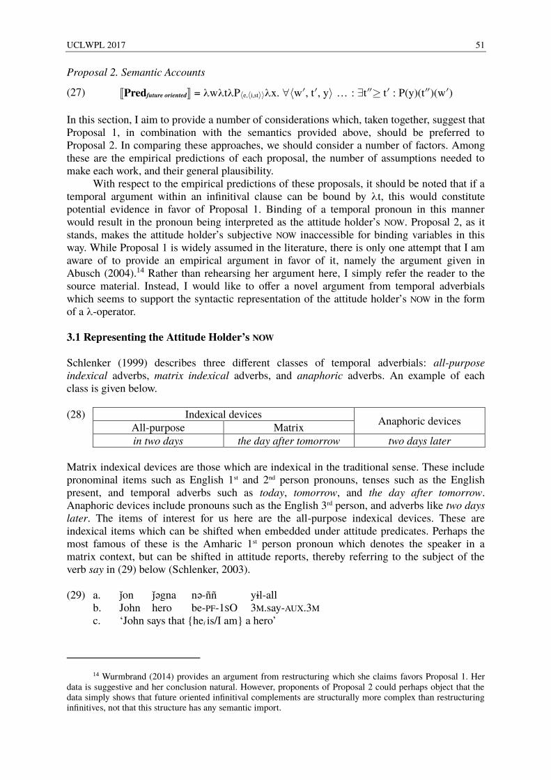
UCLWPL 2017 51

Proposal 2. Semantic Accounts

(27) ⟦Predfuture oriented⟧ = λwλtλP⟨e,⟨i,st⟩⟩λx. ∀⟨w′, t′, y⟩ … : ∃t″≥ t′ : P(y)(t″)(w′)

In this section, I aim to provide a number of considerations which, taken together, suggest that Proposal 1, in combination with the semantics provided above, should be preferred to Proposal 2. In comparing these approaches, we should consider a number of factors. Among these are the empirical predictions of each proposal, the number of assumptions needed to make each work, and their general plausibility. With respect to the empirical predictions of these proposals, it should be noted that if a temporal argument within an infinitival clause can be bound by λt, this would constitute potential evidence in favor of Proposal 1. Binding of a temporal pronoun in this manner would result in the pronoun being interpreted as the attitude holder’s NOW. Proposal 2, as it stands, makes the attitude holder’s subjective NOW inaccessible for binding variables in this way. While Proposal 1 is widely assumed in the literature, there is only one attempt that I am aware of to provide an empirical argument in favor of it, namely the argument given in Abusch (2004).14 Rather than rehearsing her argument here, I simply refer the reader to the source material. Instead, I would like to offer a novel argument from temporal adverbials which seems to support the syntactic representation of the attitude holder’s NOW in the form of a λ-operator. 3.1 Representing the Attitude Holder’s NOW Schlenker (1999) describes three different classes of temporal adverbials: all-purpose indexical adverbs, matrix indexical adverbs, and anaphoric adverbs. An example of each class is given below. (28) Indexical devices

Anaphoric devices All-purpose Matrix in two days the day after tomorrow two days later Matrix indexical devices are those which are indexical in the traditional sense. These include pronominal items such as English 1st and 2nd person pronouns, tenses such as the English present, and temporal adverbs such as today, tomorrow, and the day after tomorrow. Anaphoric devices include pronouns such as the English 3rd person, and adverbs like two days later. The items of interest for us here are the all-purpose indexical devices. These are indexical items which can be shifted when embedded under attitude predicates. Perhaps the most famous of these is the Amharic 1st person pronoun which denotes the speaker in a matrix context, but can be shifted in attitude reports, thereby referring to the subject of the verb say in (29) below (Schlenker, 2003). (29) a. ǰon ǰǝgna nǝ-ññ yil-all b. John hero be-PF-1SO 3M.say-AUX.3M c. ‘John says that {hei is/I am} a hero’

14 Wurmbrand (2014) provides an argument from restructuring which she claims favors Proposal 1. Her data is suggestive and her conclusion natural. However, proponents of Proposal 2 could perhaps object that the data simply shows that future oriented infinitival complements are structurally more complex than restructuring infinitives, not that this structure has any semantic import.

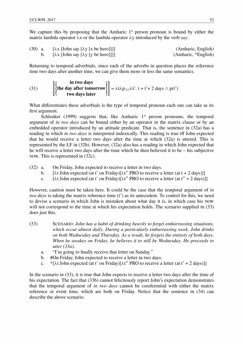
UCLWPL 2017 52

We capture this by proposing that the Amharic 1st person pronoun is bound by either the matrix lambda operator λx or the lambda operator λy introduced by the verb say. (30) a. [λx [John say [λy [x be hero]]]] (Amharic, English) b. [λx [John say [λy [y be hero]]]] (Amharic, *English) Returning to temporal adverbials, since each of the adverbs in question places the reference time two days after another time, we can give them more or less the same semantics.

(31)

⟦{in two days

the day after tomorrowtwo days later

}⟧ = λtλp⟨i,t⟩λt′. t = t′+ 2 days ∧ p(t′)

What differentiates these adverbials is the type of temporal pronoun each one can take as its first argument. Schlenker (1999) suggests that, like Amharic 1st person pronouns, the temporal argument of in two days can be bound either by an operator in the matrix clause or by an embedded operator introduced by an attitude predicate. That is, the sentence in (32a) has a reading in which in two days is interpreted indexically. This reading is true iff John expected that he would receive a letter two days after the time at which (32a) is uttered. This is represented by the LF in (32b). However, (32a) also has a reading in which John expected that he will receive a letter two days after the time which he then believed it to be – his subjective NOW. This is represented in (32c). (32) a. On Friday, John expected to receive a letter in two days. b. [λt John expected (at t′ on Friday)[λt″ PRO to receive a letter (at t + 2 days)]] c. [λt John expected (at t′ on Friday)[λt″ PRO to receive a letter (at t″ + 2 days)]] However, caution must be taken here. It could be the case that the temporal argument of in two days is taking the matrix reference time (t′) as its antecedent. To control for this, we need to devise a scenario in which John is mistaken about what day it is, in which case his NOW will not correspond to the time at which his expectation holds. The scenario supplied in (33) does just this. (33)

SCENARIO: John has a habit of drinking heavily to forget embarrassing situations, which occur almost daily. During a particularly embarrassing week, John drinks on both Wednesday and Thursday. As a result, he forgets the entirety of both days. When he awakes on Friday, he believes it to still be Wednesday. He proceeds to utter (33a).

a. “I’m going to finally receive that letter on Sunday.” b. # On Friday, John expected to receive a letter in two days. c. * [λt John expected (at t′ on Friday)[λt″ PRO to receive a letter (at t′ + 2 days)]] In the scenario in (33), it is true that John expects to receive a letter two days after the time of his expectation. The fact that (33b) cannot felicitously report John’s expectation demonstrates that the temporal argument of in two days cannot be coreferential with either the matrix reference or event time, which are both on Friday. Notice that the sentence in (34) can describe the above scenario.

UCLWPL 2017 53

(34) SCENARIO: Same as (33). a. On Friday, John expected to receive a letter in four days. This is expected if the adverbial in n days can be interpreted as n days from the attitude holder’s subjective NOW, which for John is Wednesday. Compare this to the anaphoric device two days later which can be interpreted with respect to the matrix reference time. (35) SCENARIO: Same as (33). a. On Friday, John expected to receive a letter two days later. b. [λt John expected (at t′ on Friday)[λt″ PRO to receive a letter (at t′ + 2 days)]] The above has shown that the adverbial in n days can have a “matrix” indexical reading and a shifted, or “all-purpose”, indexical reading. In the former case, the adverb picks out the time two days after the utterance time, while in the latter case, it picks out the time two days after the attitude holder’s subjective NOW. This suggests that, at the very least, we need to represent the NOW of the attitude holder syntactically in future oriented infinitives. However, it does not necessarily show that the infinitival needs to contain a covert operator per se.15 In the following section, I briefly review two specific accounts which attempt to do away with covert future operators by treating the selecting predicates as quantifiers over times. 3.2 Accounts sans Operators 3.2.1 Katz (2001). In order to avoid wrongly generating future readings in SOT complements to expect, Katz (2001) suggests that expect not only controls the top most time variable, but also lexically specifies precedence between the attitude holder’s NOW and the embedded reference time (36).

(36) ⟦expectKatz⟧ = λwλtλP⟨e,⟨i,⟨i,st⟩⟩⟩λx. ∀⟨w′, t′, y⟩ ∈ Doxx,t,w : ∃t″> t′ : P(y)(t′)(t″)(w′)

Katz maintains that expect can never take a non-future complement. For him, simultaneous finite complements are highly marginal.16 He suggests that, for those speakers who allow it, the verb expect is ambiguous and when it takes a simultaneous complement it means something akin to “strongly believe” (fn.1). Let us grant that for some speakers expect may always be future oriented. If so, we still need to propose covert operators in infinitival complements to hope. To see why, consider the fact that hope can embed present tense, SOT, and past tense finite complements (37a,b,c) as well as future oriented infinitives (37d). (37) a. We hope you’re feeling better now. b. John hoped that Mary was still alive. (SOT) c. I hope you arrived home safely last night. d. John hopes to receive a letter in two days.

15 In response to an earlier version of this work, Pearson (2017) includes an additional lambda-abstractor corresponding to the attitude holder’s NOW in the embedded clause. This proposal is also adopted by Katz (2001) for independent reasons. In the following two subsections (3.2.1, 3.2.2.), it will be shown that, even with this assumption, these proposals face a number of problems.

16 This judgement does not appear to be widely shared in the literature or among the speakers I consulted.

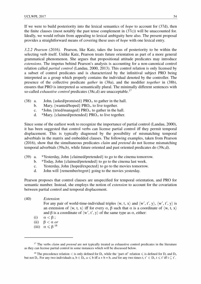
UCLWPL 2017 54

If we were to build posteriority into the lexical semantics of hope to account for (37d), then the finite clauses (most notably the past tense complement in (37c)) will be unaccounted for. Ideally, we would refrain from appealing to lexical ambiguity here also. The present proposal provides a straightforward means of covering these uses of hope with one lexical entry. 3.2.2 Pearson (2016). Pearson, like Katz, takes the locus of posteriority to be within the selecting verb itself. Unlike Katz, Pearson treats future orientation as part of a more general grammatical phenomenon. She argues that propositional attitude predicates may introduce extensions. The impetus behind Pearson’s analysis is accounting for a non-canonical control relation called partial control (Landau, 2000, 2013). This control relation is only licensed by a subset of control predicates and is characterized by the infinitival subject PRO being interpreted as a group which properly contains the individual denoted by the controller. The presence of the collective predicate gather in (38a), and the modifier together in (38b), ensures that PRO is interpreted as semantically plural. The minimally different sentences with so-called exhaustive control predicates (38c,d) are unacceptable.17 (38) a. Johni {asked/promised} PROi+ to gather in the hall. b. Maryi {wanted/hoped} PROi+ to live together. c. * Johni {tried/managed} PROi+ to gather in the hall. d. * Maryi {claimed/pretended} PROi+ to live together. Since some of the earliest work to recognize the importance of partial control (Landau, 2000), it has been suggested that control verbs can license partial control iff they permit temporal displacement. This is typically diagnosed by the possibility of mismatching temporal adverbials in the matrix and embedded clauses. The following examples, taken from Pearson (2016), show that the simultaneous predicates claim and pretend do not license mismatching temporal adverbials (39a,b), while future oriented and past oriented predicates do (39c,d). (39) a. * Yesterday, John {claimed/pretended} to go to the cinema tomorrow. b. * Today, John {claimed/pretended} to go to the cinema last week. c. Yesterday, John {hoped/expected} to go to the movies tomorrow. d. John will {remember/regret} going to the movies yesterday. Pearson proposes that control clauses are unspecified for temporal orientation, and PRO for semantic number. Instead, she employs the notion of extension to account for the covariation between partial control and temporal displacement. (40) Extension

For any pair of world-time-individual triples ⟨w, t, x⟩ and ⟨w′, t′, y⟩, ⟨w′, t′, y⟩ is an extension of ⟨w, t, x⟩ iff for every α, β such that α is a coordinate of ⟨w, t, x⟩ and β is a coordinate of ⟨w′, t′, y⟩ of the same type as α, either:

(i) α < β ; (ii) β < α or

(iii) α ⩽ β 18

17 The verbs claim and pretend are not typically treated as exhaustive control predicates in the literature as they can license partial control in some instances which will be discussed below.

18 The precedence relation < is only defined for Di, while the ‘part of’ relation ⩽ is defined for De and Di, but not Ds. For any two individuals a, b ∈ De, a ⩽ b iff a + b = b, and for any two times t, t′ ∈ Di, t ⩽ t′ iff t ⊆ t′.

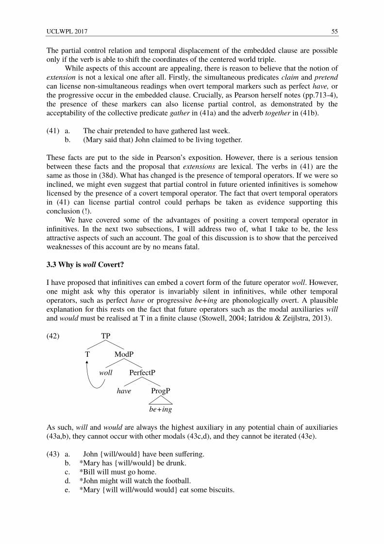
UCLWPL 2017 55

The partial control relation and temporal displacement of the embedded clause are possible only if the verb is able to shift the coordinates of the centered world triple. While aspects of this account are appealing, there is reason to believe that the notion of extension is not a lexical one after all. Firstly, the simultaneous predicates claim and pretend can license non-simultaneous readings when overt temporal markers such as perfect have, or the progressive occur in the embedded clause. Crucially, as Pearson herself notes (pp.713-4), the presence of these markers can also license partial control, as demonstrated by the acceptability of the collective predicate gather in (41a) and the adverb together in (41b). (41) a. The chair pretended to have gathered last week. b. (Mary said that) John claimed to be living together. These facts are put to the side in Pearson’s exposition. However, there is a serious tension between these facts and the proposal that extensions are lexical. The verbs in (41) are the same as those in (38d). What has changed is the presence of temporal operators. If we were so inclined, we might even suggest that partial control in future oriented infinitives is somehow licensed by the presence of a covert temporal operator. The fact that overt temporal operators in (41) can license partial control could perhaps be taken as evidence supporting this conclusion (!). We have covered some of the advantages of positing a covert temporal operator in infinitives. In the next two subsections, I will address two of, what I take to be, the less attractive aspects of such an account. The goal of this discussion is to show that the perceived weaknesses of this account are by no means fatal. 3.3 Why is woll Covert? I have proposed that infinitives can embed a covert form of the future operator woll. However, one might ask why this operator is invariably silent in infinitives, while other temporal operators, such as perfect have or progressive be+ing are phonologically overt. A plausible explanation for this rests on the fact that future operators such as the modal auxiliaries will and would must be realised at T in a finite clause (Stowell, 2004; Iatridou & Zeijlstra, 2013).

(42) TP T ModP woll PerfectP have ProgP be + ing As such, will and would are always the highest auxiliary in any potential chain of auxiliaries (43a,b), they cannot occur with other modals (43c,d), and they cannot be iterated (43e). (43) a. John {will/would} have been suffering. b. * Mary has {will/would} be drunk. c. * Bill will must go home. d. * John might will watch the football. e. * Mary {will will/would would} eat some biscuits.

UCLWPL 2017 56

Taken together, these facts entail that, in a finite clause, they will always be the verbal element bearing finiteness. Perhaps for this reason, modal auxiliaries lack an overt non-finite form (*to will/would/woll). Conversely, have and be+ing frequently occur inside auxiliary chains and thus have readily available non-finite forms. It would not be unreasonable then to propose that the future operator woll can, and indeed does, occur in infinitives. However, it cannot be spelled out there because it lacks an appropriate non-finite form.19 3.4 Transitive Constructions Another prima facie advantage of a semantic account (Proposal 2) over a syntactic account (Proposal 1) is that verbs such as expect are future oriented even in transitive constructions. For instance, there appears to be no clausal complement to expect in (44) yet the expectation still seems concerned with a future event (i.e., getting a cheque). (44) John is expecting a cheque. There is a long tradition of analyzing Intensional Transitive Verbs (ITVs) in construction such as this as selecting a covert clausal complement which features a covert predicate ⌀have/get (Ross, 1976; Dikken et al., 1996; Larson et al., 1997; Harley, 2004 inter alia). (45) Johni is expecting [PROi have/get a cheque]. The motivation for this type of analysis is extensive and well-documented (see references above). But we can consider just two of the more straightforward pieces of evidence. Firstly, (46) shows that transitive expect can license two mismatching temporal adverbials (McCawley, 1979), typically taken to be indicative of bi-clausal structure. (46) Yesterday, Johni was expecting [PROi have/get a cheque next week]. The frame adverbial yesterday restricts the time of the expectation, while next week is modifying some covert event which can be paraphrased by to get a cheque. The second piece of evidence exploits a scope ambiguity which arises with the adverb again. Consider the following scenario. (47)

SCENARIO: John is being sued for a second time. The first time he got sued, it was a surprise, as he was not expecting it. This time, however, he is not surprised.

a. John was expecting a law suit again. The reading on which again modifies the matrix verb is false in this scenario because at no point before did John expect a lawsuit. The felicitous reading is one on which again modifies the covert predicate have/get. Provided we take these arguments to be convincing, we have good reason to propose a covert clause in ITV constructions. This is equally true for both Proposal 1 and Proposal 2. The only further assumption that we need to make is that this covert clause can host a covert future operator. If so, then, contrary to appearances, transitive constructions do not necessarily favor a semantic account (Proposal 2) over a syntactic account (Proposal 1).

19 There are a number of instances in which infinitives receive a clearly modal interpretation, while nonetheless lacking an overt modal element (see for instance Bhatt, 2006 and White, 2014). It remains to be seen whether these instances of covert modality might receive a similar explanation.

UCLWPL 2017 57

4 Discussion and Conclusion Portner (to appear) rightly observes that semantic research into the temporal orientation of infinitives is still only fragmentary. And it is certainly true that the majority of work on infinitival tense is primarily concerned with the status of the infinitival subject (i.e., PRO, trace, or ECM subject), with only secondary interest in temporality (e.g., Stowell, 1982; Pesetsky, 1992; Landau, 2000; Martin, 2001; Grano, 2015; Pearson, 2016). In the ideal scenario, we would posit as little as possible (e.g., one future operator), with the temporal readings following from other independently motivated principles. I have tried to show how this might look in the case of a few verbs which license both a future and simultaneous reading. However, there are several predicates which are obligatorily future oriented (e.g., promise, decide), and others which select infinitives with obligatorily simultaneous readings (e.g., claim, pretend, be glad). The point of this paper has been to suggest that what dictates the temporal orientation of infinitival complements is not temporal semantics of the selecting verb per se, but rather other independently motivated aspects of the verb’s lexical semantics plus an optional future operator. This logic would suggest that there is some feature of the lexical semantics of obligatorily simultaneous predicates which rules out the embedding of the future operator, while the lexical semantics of obligatorily future oriented predicates necessitates the presence of a future operator. I believe that such an approach could prove to be promising in future research on this matter. References Abusch, D. (1998). Generalizing Tense Semantics for Future Contexts. Events and Grammar, (5), 13–33. Abusch, D. (2004). On the Temporal Composition of Infinitives. In J. Gueron & J. Lecarme (Eds.), The syntax

of time (pp. 27–53). MIT Press. Anand, P., & Hacquard, V. (2013). Epistemics and attitudes. Semantics and Pragmatics, 6(8), 1–59. Retrieved

from http://semprag.org/article/view/sp.6.8 Bhatt, R. (2006). Covert modality in non-finite contexts. Berlin: Mouton de Gruyter. Bresnan, J. (1972). Theory of complementation in English syntax. MIT. Chierchia, G. (1989). Anaphora and Attitudes “De Se.” In B. van Benthem & B. van Emde (Eds.), Semantics

and Contextual Expressions (pp. 1–31). Dordrecht: Kluwer. Dikken, M. den, Larson, R., & Ludlow, P. (1996). Intensional “transitive” verbs and concealed complement

clauses. Rivista Di Linguistica, 8, 331–48. Grano, T. (2015). Control and Restructuring. New York: Oxford University Press. Harley, H. (2004). Wanting, Having and Getting: A Note on Fodor and Lepore 1998. Linguistic Inquiry, 35(2),

255–267. Hegarty, M. (2016). Modality and Propositional Attitudes. Cambridge: Cambridge University Press. Heim, I. (1992). Presupposition projection and the semantics of attitude verbs. Journal of Semantics, 9(3), 183–

221. Iatridou, S., & Zeijlstra, H. (2013). Negation, Polarity, and Deontic Modals. Linguistic Inquiry, 44(4), 529–568.

Retrieved from http://www.mitpressjournals.org/doi/10.1162/LING_a_00138 Katz, G. (2001). ( A ) temporal Complements. In C. Féry & W. Sternefeld (Eds.), Audiatur Vox Sapientiae (pp.

240–258). Berlin: Akademie. Kratzer, A. (1977). What “must” and “can” must and can mean. Linguistics and Philosophy, 1, 337–355. Kratzer, A. (1981). The notional category of modality. In H. J. Eikmeyer & H. Rieser (Eds.), Words, Worlds and

Contexts (pp. 38–74). Berlin: de Gruyter. Kratzer, A. (2012). Modals and Conditionals: New and Revised Perspectives. Modals and Conditionals: New

and Revised Perspectives. https://doi.org/10.1093/acprof:oso/9780199234684.001.0001 Landau, I. (2000). Elements of Control: Structure and Meaning in Infinitival Constructions. Dordrecht,

Netherlands: Kluwer Academic Publishers. Landau, I. (2013). Control in generative grammar: A research companion. Cambridge: Cambridge University

Press.

UCLWPL 2017 58

Larson, R., Dikken, M. Den, & Ludlow, P. (1997). Intensional Transitive Verbs and Abstract Clausal Complementation. Retrieved from https://linguistics.stonybrook.edu/sites/default/files/uploads/u18/publications/ITVs-OUP%28rev-final%29.pdf

Lewis, D. (1979). Attitudes de dicto and de se. Philosophical Review, 88(4), 513–543. Lyons, J. (1977). Semantics Vol. 2. Cambridge: Cambridge University Press. Martin, R. (2001). Null Case and the Distribution of PRO. Linguistic Inquiry, 32Martin,(1), 141–166. McCawley, J. (1979). On identifying the remains of deceased clauses. In J. McCawley (Ed.), Adverbs, Vowels,

and Other Objects of Wonder (pp. 84–95). Chicago: Univeristy of Chicago Press. Papafragou, A. (2006). Epistemic modality and truth conditions. Lingua, 116(10), 1688–1702. Pearson, H. (2016). The semantics of partial control. Natural Language and Linguistic Theory, 34(2), 691–738.

Retrieved from http://dx.doi.org/10.1007/s11049-015-9313-9 Pearson, H. (2017). Revisiting Tense and Aspect in English Infinitives. Presented at Tenselessness Workshop,

Univeristy of Greenwich. Pesetsky, D. (1992). Zero syntax II: an essay on infinitives. Ms., MIT. Portner, P. (2009). Modality. Oxford: Oxford University Press. Portner, P. (to appear). Mood. Oxford: Oxford University Press. Ross, J. (1976). To “have” and not to “have.” In M. A. Jazayery, E. C. Polomé, & W. Winter (Eds.), Linguistic

and Literary Studies in Honor of Archibald A. Hill (pp. 263–70). The Hague: Mouton. Rubinstein, A. (2012). Roots of Modality. University of Massachusetts - Amherst. Scheffler, T. (2008). Semantic operators in different dimensions. Philadelphia, PA. Schlenker, P. (1999). Propositional attitudes and indexicality: A cross categorial approach. MIT. Schlenker, P. (2003). A Plea for Monsters. Linguistics and Philosophy, 26(1), 29–120. Stalnaker, R. (1978). Assertion. Syntax and Semantics, (9), 315–332. Stephenson, T. (2007). Towards a Theory of Subjective Meaning by. MIT. Stowell, T. (1982). The Tense of Infinitives. Linguistic Inquiry, 13(3), 561–570. Stowell, T. (2004). Tense and modals. In J. Gueron & J. Lecarme (Eds.), The syntax of time (pp. 621–635).

Cambridge, MA: MIT Press. Stowell, T. (2007). Sequence of Perfect. In L. de Saussure, J. Moeschler, & G. Puskas (Eds.), Recent advances

in the syntax and semantics of tense, mood and aspect (Vol. 185, pp. 123–146). Berlin: Mouton de Gruyter.

Uegaki, W. (2011). “Nearly free” control as an underspecified de se report. In O. Bonami & P. Cabredo Hofherr (Eds.), Empirical Issues in Syntax and Semantics 8 (Proceedings of CSSP 2009). (pp. 511–536). Retrieved from http://www.cssp.cnrs.fr/eiss8

von Fintel, K. (1999). NPI Licensing, Strawson Entailment, and Context Dependency. Journal of Semantics, 16(2), 97–148. https://doi.org/10.1093/jos/16.2.97

White, A. S. (2014). Factive implicatives and modalised complements. NELS 44: Proceesings from the 44th meeting of the North East Linguistics Society, Amherst.

Wurmbrand, S. (2014). Tense and apsect in English infinitives. Linguistic Inquiry, 45(3), 403–447.