Gradually Varied Flow I+II

Hydromechanics VVR090

Gradually Varied Flow

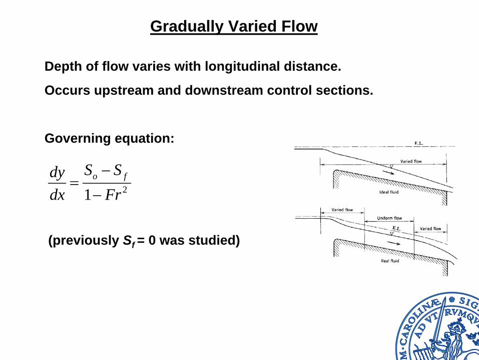
Depth of flow varies with longitudinal distance.

Occurs upstream and downstream control sections.

Governing equation:

21−

=−o fS Sdy

dx Fr

(previously Sf = 0 was studied)

Derivation of Governing Equation

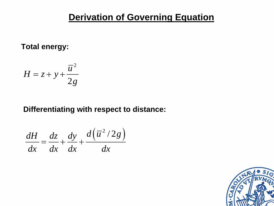
Total energy:

2

2uH z yg

= + +

Differentiating with respect to distance:

( )2 / 2= + +

d u gdH dz dydx dx dx dx

= −

= −

f

o

dH Sdx

dz Sdx

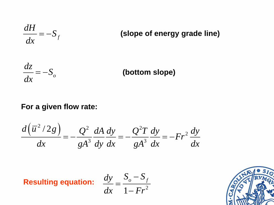
For a given flow rate:

( )2 2 22

3 3

/ 2d u g Q dA dy Q T dy dyFrdx gA dy dx gA dx dx

= − = − = −

(slope of energy grade line)

(bottom slope)

21−

=−o fS Sdy

dx FrResulting equation:

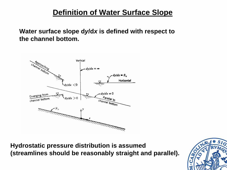
Definition of Water Surface Slope

Water surface slope dy/dx is defined with respect to the channel bottom.

Hydrostatic pressure distribution is assumed (streamlines should be reasonably straight and parallel).

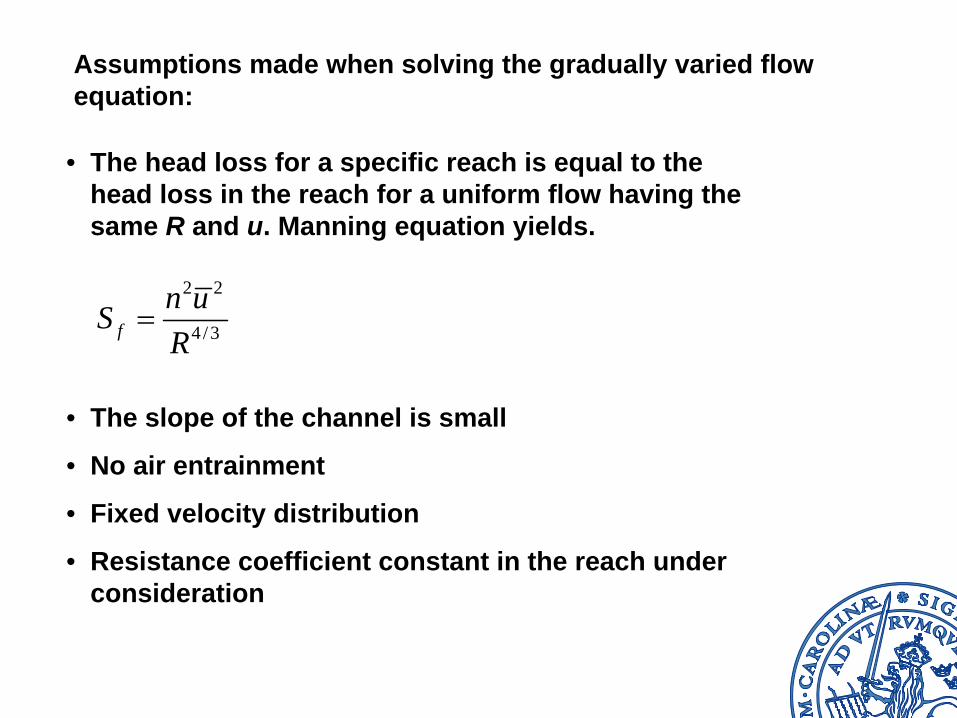
• The head loss for a specific reach is equal to the head loss in the reach for a uniform flow having the same R and u. Manning equation yields.

• The slope of the channel is small

• No air entrainment

• Fixed velocity distribution

• Resistance coefficient constant in the reach under consideration

2 2

4/3fn uSR

=

Assumptions made when solving the gradually varied flow equation:

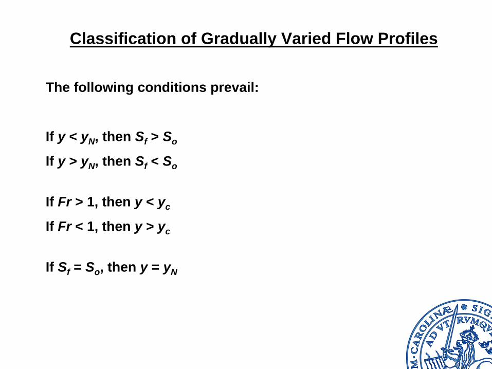
Classification of Gradually Varied Flow Profiles

The following conditions prevail:

If y < yN , then Sf > So

If y > yN , then Sf < So

If Fr > 1, then y < yc

If Fr < 1, then y > yc

If Sf = So , then y = yN

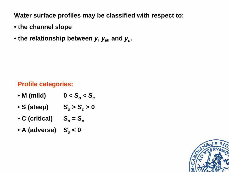
Water surface profiles may be classified with respect to:

• the channel slope

• the relationship between y, yN , and yc .

Profile categories:

• M (mild) 0 < So < Sc

• S (steep) So > Sc > 0

• C (critical) So = Sc

• A (adverse) So < 0

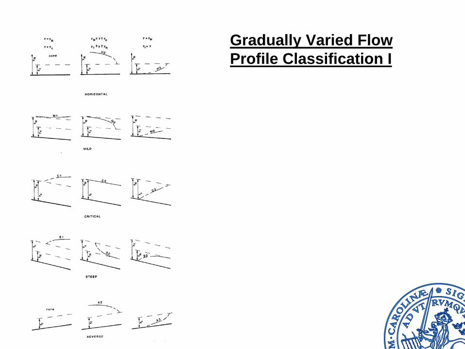
Gradually Varied Flow Profile Classification I

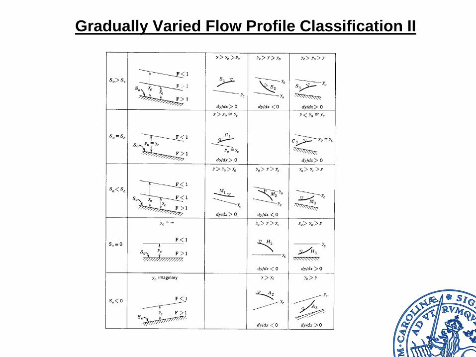
Gradually Varied Flow Profile Classification II

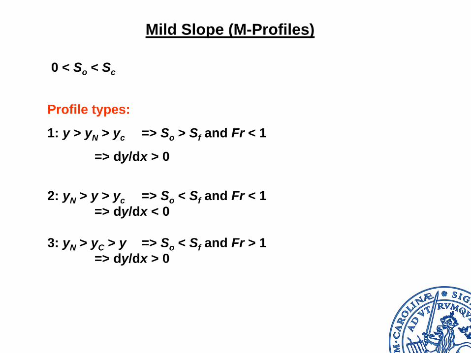
Mild Slope (M-Profiles)

Profile types:

1: y > yN > yc => So > Sf and Fr < 1

=> dy/dx > 0

2: yN > y > yc => So < Sf and Fr < 1=> dy/dx < 0

3: yN > yC > y => So < Sf and Fr > 1=> dy/dx > 0

0 < So < Sc

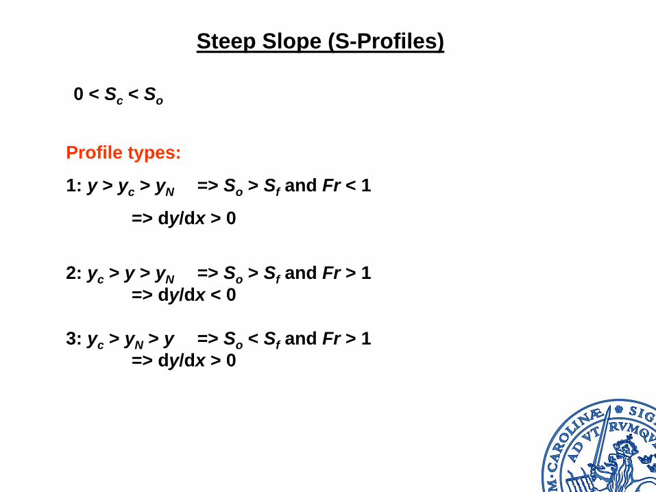
Steep Slope (S-Profiles)

Profile types:

1: y > yc > yN => So > Sf and Fr < 1

=> dy/dx > 0

2: yc > y > yN => So > Sf and Fr > 1=> dy/dx < 0

3: yc > yN > y => So < Sf and Fr > 1=> dy/dx > 0

0 < Sc < So

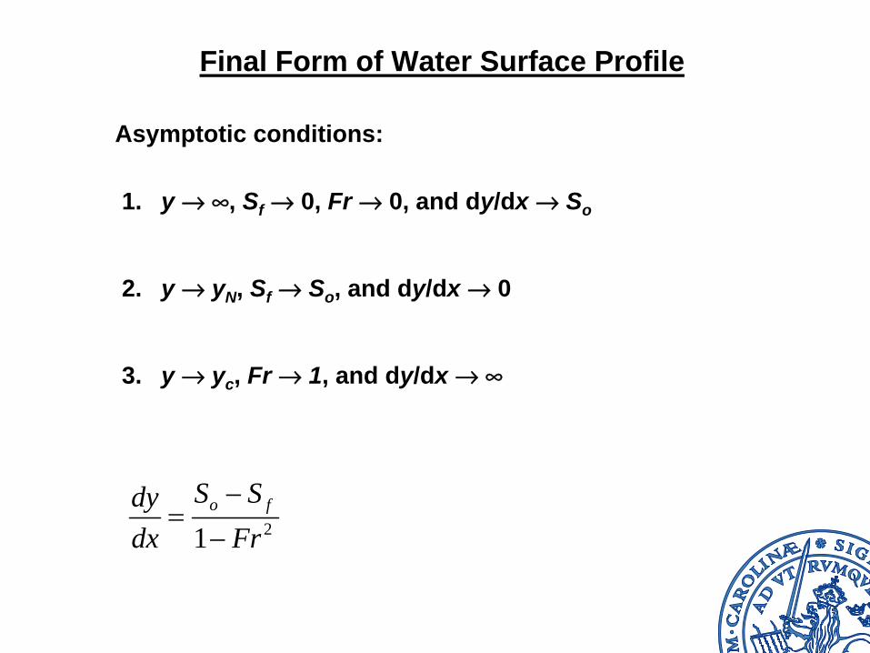
Final Form of Water Surface Profile

1. y Æ •, Sf Æ 0, Fr Æ 0, and dy/dx Æ So

2. y Æ yN , Sf Æ So , and dy/dx Æ 0

3. y Æ yc , Fr Æ 1, and dy/dx Æ •

21−

=−o fS Sdy

dx Fr

Asymptotic conditions:

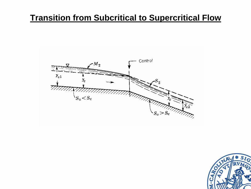
Transition from Subcritical to Supercritical Flow

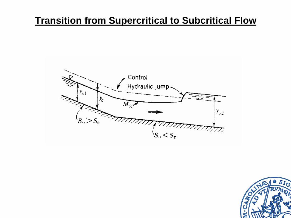
Transition from Supercritical to Subcritical Flow

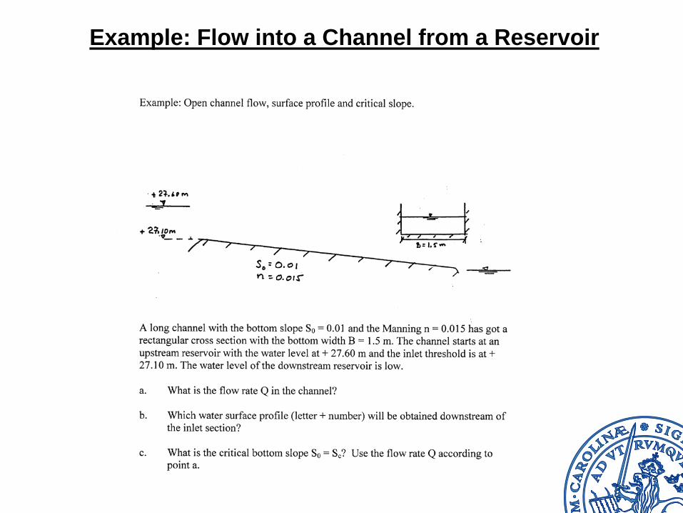
Example: Flow into a Channel from a Reservoir

Flow Controls

• determine the depth in channel either upstream or downstream such points.

• usually feature a change from subcritical to supercritical flow

• occur at physical barriers, for example, sluice gates, dams, weirs, drop structures, or changes in channel slope

Locations in the channel where the relationship between the water depth and flow rate is known (or controllable).

Controls:

Strategy for Analysis of Open Channel Flow

1. Start at control points

2. Proceed upstream or downstream depending on whether subcritical or supercritical flow occurs, respectively

Typical approach in the analysis:

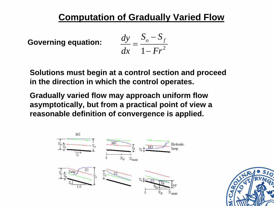
Computation of Gradually Varied Flow

21−

=−o fS Sdy

dx FrGoverning equation:

Solutions must begin at a control section and proceed in the direction in which the control operates.

Gradually varied flow may approach uniform flow asymptotically, but from a practical point of view a reasonable definition of convergence is applied.

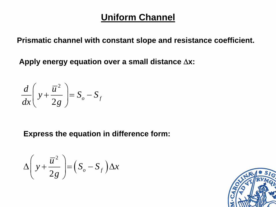
Uniform Channel

Prismatic channel with constant slope and resistance coefficient.

Apply energy equation over a small distance Dx:

2

2 o fd uy S Sdx g

⎛ ⎞+ = −⎜ ⎟

⎝ ⎠

Express the equation in difference form:

( )2

2 o fuy S S xg

⎛ ⎞Δ + = − Δ⎜ ⎟⎝ ⎠

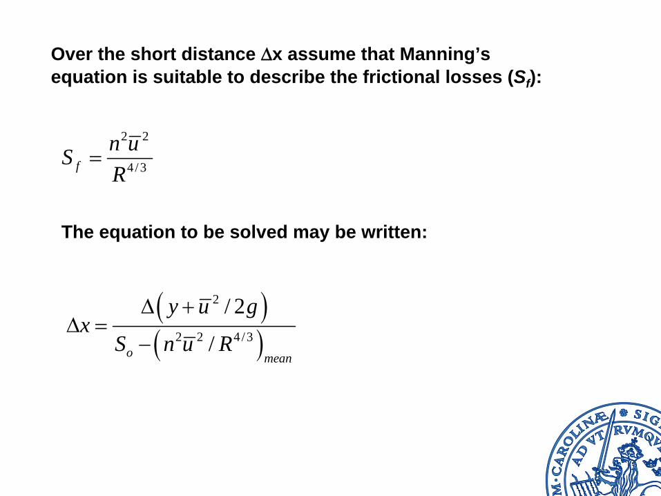
Over the short distance Dx assume that Manning’s equation is suitable to describe the frictional losses (Sf ):

2 2

4/3fn uSR

=

The equation to be solved may be written:

( )( )

2

2 2 4 /3

/ 2

/o mean

y u gx

S n u R

Δ +Δ =

−

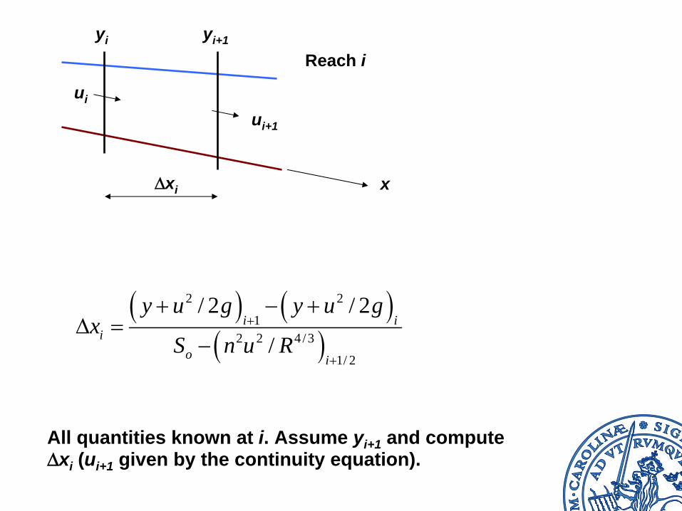
Dxi

Reach i

x

yi yi+1

( ) ( )( )

2 2

12 2 4/3

1/ 2

/ 2 / 2

/i i

io i

y u g y u gx

S n u R+

+

+ − +Δ =

−

All quantities known at i. Assume yi+1 and compute Dxi (ui+1 given by the continuity equation).

ui

ui+1

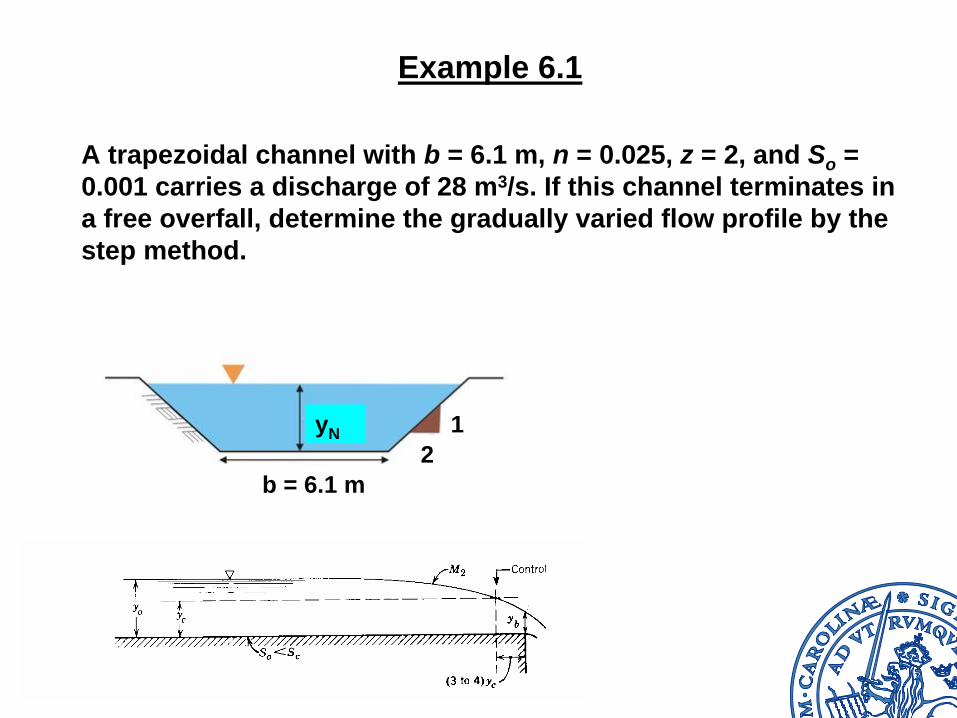
Example 6.1

A trapezoidal channel with b = 6.1 m, n = 0.025, z = 2, and So = 0.001 carries a discharge of 28 m3/s. If this channel terminates in a free overfall, determine the gradually varied flow profile by the step method.

b = 6.1 m2

1yN

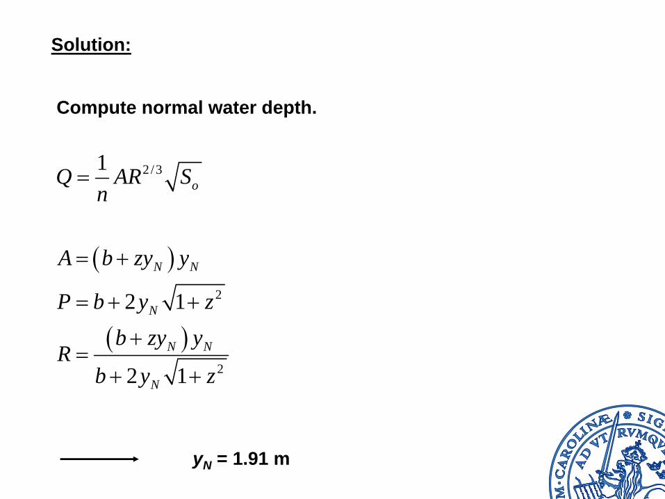
Solution:

Compute normal water depth.

( )

( )

2/3

2

2

1

2 1

2 1

o

N N

N

N N

N

Q AR Sn

A b zy y

P b y zb zy y

Rb y z

=

= +

= + +

+=

+ +

yN = 1.91 m

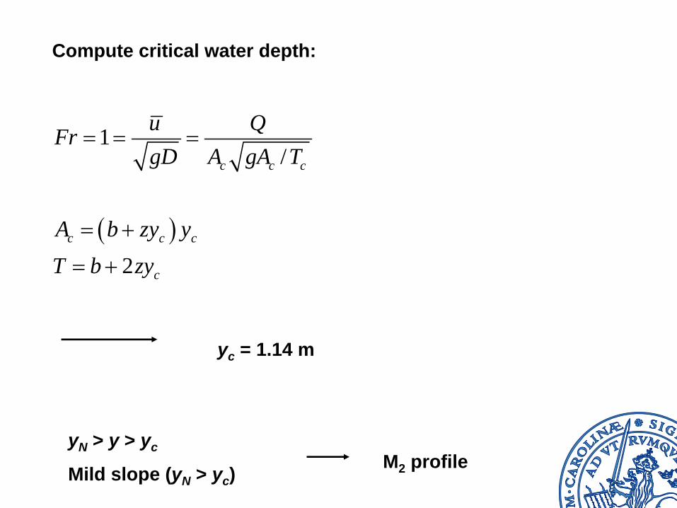
Compute critical water depth:

( )

1/

2

c c c

c c c

c

u QFrgD A gA T

A b zy yT b zy

= = =

= +

= +

yc = 1.14 m

yN > y > yc

Mild slope (yN > yc )M2 profile

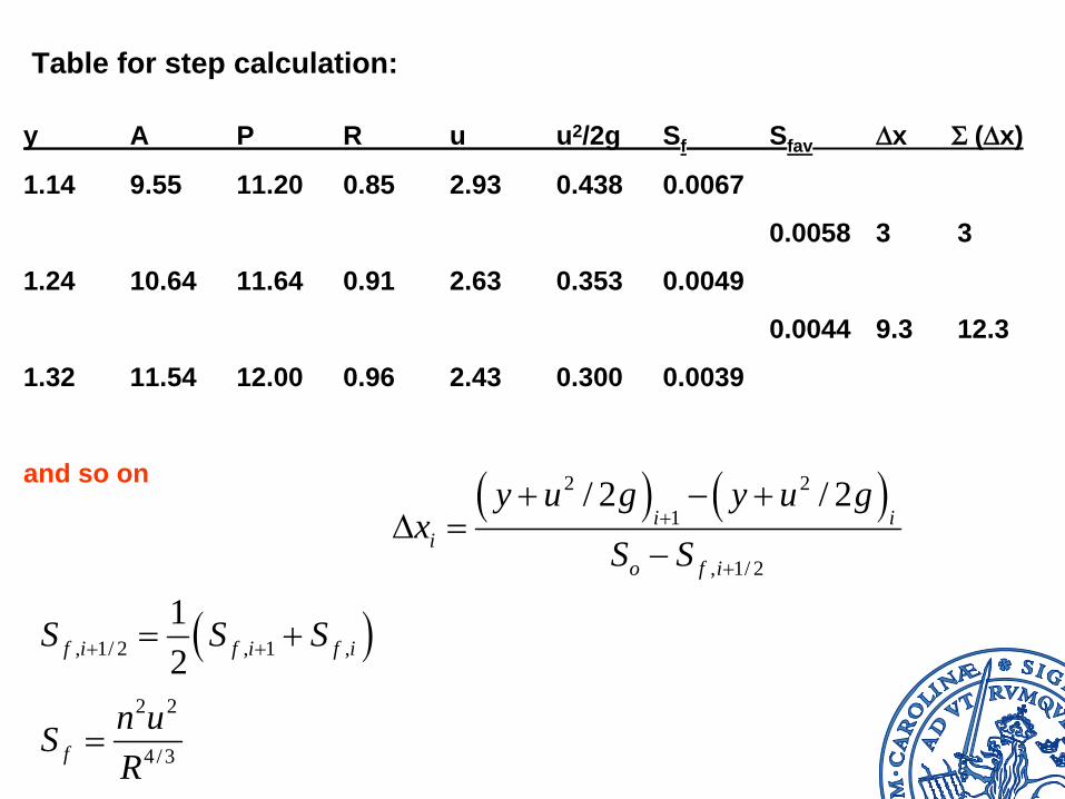
Table for step calculation:

y A P R u u2/2g Sf Sfav Dx S

(Dx)

1.14 9.55 11.20 0.85 2.93 0.438 0.0067

0.0058 3 3

1.24 10.64 11.64 0.91 2.63 0.353 0.0049

0.0044 9.3 12.3

1.32 11.54 12.00 0.96 2.43 0.300 0.0039

and so on ( ) ( )2 2

1

, 1/ 2

/ 2 / 2i i

io f i

y u g y u gx

S S+

+

+ − +Δ =

−

( ), 1/ 2 , 1 ,12f i f i f iS S S+ += +

2 2

4/3fn uSR

=

Other Solution Methods

Problem with the step method is that the water depths is obtained at arbitrary locations (i.e., the water depth is not calculated at fixed x-locations).

By direct integration of the governing equation this problem can be circumvented.

Different approaches for direct integration:

• semi-analytic

• trial-and-error

• finite difference

Semi-Analytic Approach

Find solution in terms of closed-form functions (integrals).

Employ suitable approximations to these functions or some look-up tables.

Approach OK for channels with constant properties.

(for more information, see French)

Trial-and-Error Approach

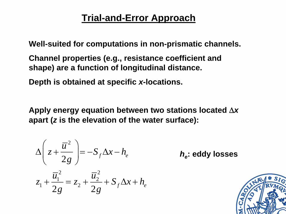
Well-suited for computations in non-prismatic channels.

Channel properties (e.g., resistance coefficient and shape) are a function of longitudinal distance.

Depth is obtained at specific x-locations.

Apply energy equation between two stations located Dx apart (z is the elevation of the water surface):

2

2 21 2

1 2

2

2 2

f e

f e

uz S x hg

u uz z S x hg g

⎛ ⎞Δ + = − Δ −⎜ ⎟⎝ ⎠

+ = + + Δ +

he : eddy losses

Equation is solved by trial-and-error (from 2 to 1):

1. Assume y1 Æ u1 (continuity equation)

2. Compute Sf (and he , if needed)

3. Compute y1 from governing equation. If this value agrees with the assumed y1 , the solution has been found. Otherwise continue calculations.

Estimate of frictional losses:

( )1 212f f fS S S= +

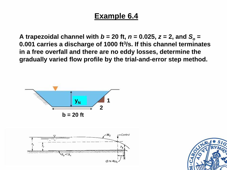
Example 6.4

A trapezoidal channel with b = 20 ft, n = 0.025, z = 2, and So = 0.001 carries a discharge of 1000 ft3/s. If this channel terminates in a free overfall and there are no eddy losses, determine the gradually varied flow profile by the trial-and-error step method.

b = 20 ft2

1yN

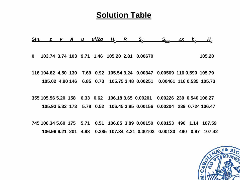
Solution Table

Stn. z y A u u2/2g H1 R Sf Sfav Dx hf H2

0 103.74 3.74 103 9.71 1.46 105.20 2.81 0.00670 105.20

116 104.62 4.50 130 7.69 0.92 105.54 3.24 0.00347 0.00509 116 0.590 105.79

105.02 4.90 146 6.85 0.73 105.75 3.48 0.00251 0.00461 116 0.535 105.73

355 105.56 5.20 158 6.33 0.62 106.18 3.65 0.00201 0.00226 239 0.540 106.27

105.93 5.32 173 5.78 0.52 106.45 3.85 0.00156 0.00204 239 0.724 106.47

745 106.34 5.60 175 5.71 0.51 106.85 3.89 0.00150 0.00153 490 1.14 107.59

106.96 6.21 201 4.98 0.385 107.34 4.21 0.00103 0.00130 490 0.97 107.42

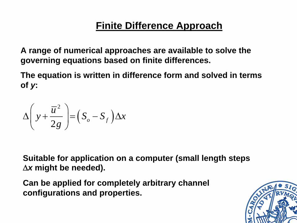
Finite Difference Approach

Suitable for application on a computer (small length steps Dx might be needed).

Can be applied for completely arbitrary channel configurations and properties.

A range of numerical approaches are available to solve the governing equations based on finite differences.

The equation is written in difference form and solved in terms of y:

( )2

2 o fuy S S xg

⎛ ⎞Δ + = − Δ⎜ ⎟⎝ ⎠

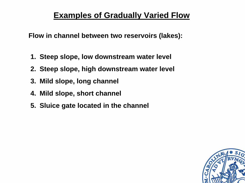
Examples of Gradually Varied Flow

Flow in channel between two reservoirs (lakes):

1. Steep slope, low downstream water level

2. Steep slope, high downstream water level

3. Mild slope, long channel

4. Mild slope, short channel

5. Sluice gate located in the channel

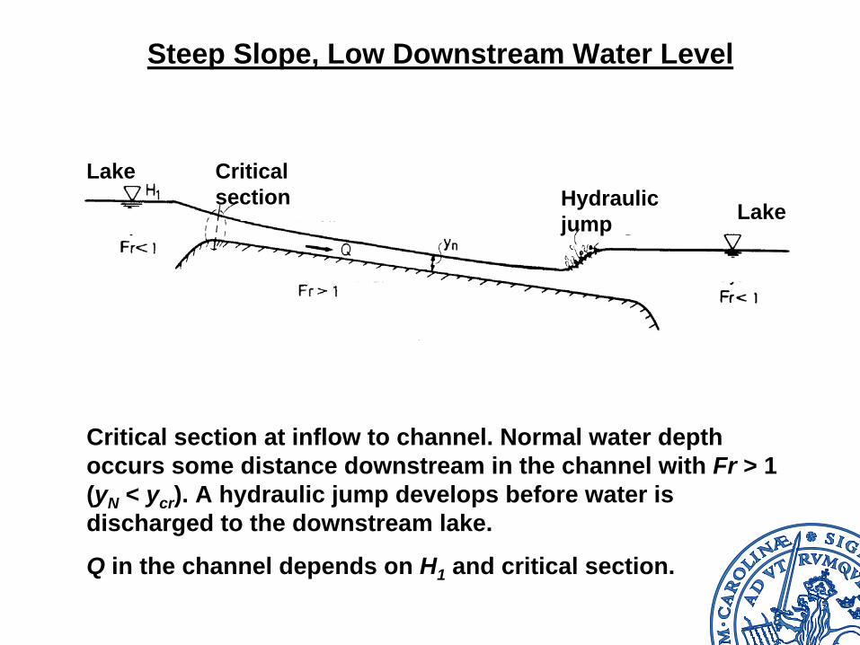
Steep Slope, Low Downstream Water Level

Critical section at inflow to channel. Normal water depth occurs some distance downstream in the channel with Fr > 1 (yN < ycr ). A hydraulic jump develops before water is discharged to the downstream lake.

Q in the channel depends on H1 and critical section.

Critical section Hydraulic

jump

Lake

Lake

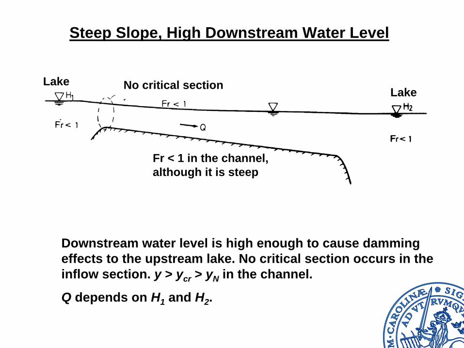
Steep Slope, High Downstream Water Level

Downstream water level is high enough to cause damming effects to the upstream lake. No critical section occurs in the inflow section. y > ycr > yN in the channel.

Q depends on H1 and H2 .

No critical section

Fr < 1 in the channel, although it is steep

LakeLake

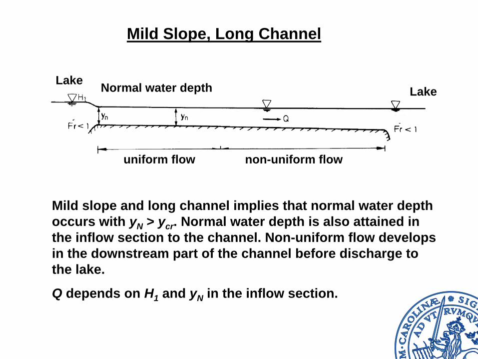
Mild Slope, Long Channel

Mild slope and long channel implies that normal water depth occurs with yN > ycr . Normal water depth is also attained in the inflow section to the channel. Non-uniform flow develops in the downstream part of the channel before discharge to the lake.

Q depends on H1 and yN in the inflow section.

LakeLake

uniform flow non-uniform flow

Normal water depth

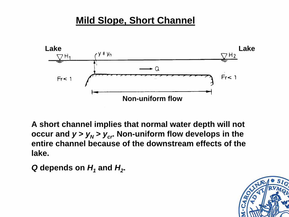
Mild Slope, Short Channel

A short channel implies that normal water depth will not occur and y > yN > ycr . Non-uniform flow develops in the entire channel because of the downstream effects of the lake.

Q depends on H1 and H2 .

Lake Lake

Non-uniform flow

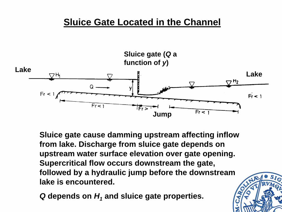
Sluice Gate Located in the Channel

Sluice gate cause damming upstream affecting inflow from lake. Discharge from sluice gate depends on upstream water surface elevation over gate opening. Supercritical flow occurs downstream the gate, followed by a hydraulic jump before the downstream lake is encountered.

Q depends on H1 and sluice gate properties.

Jump

Sluice gate (Q a function of y)

Lake Lake

Calculation Procedure for Some Gradually Varied Flows

1. Flow from a reservoir to a long, steeply sloping channel

2. Flow from a reservoir to a long, mildly sloping channel

3. Flow from a reservoir to a short, mildly sloping channel where a downstream water level affects the flow in the channel

4. Flow from a reservoir to a short, steeply sloping channel where a downstream water level affects the flow in the channel

Lake

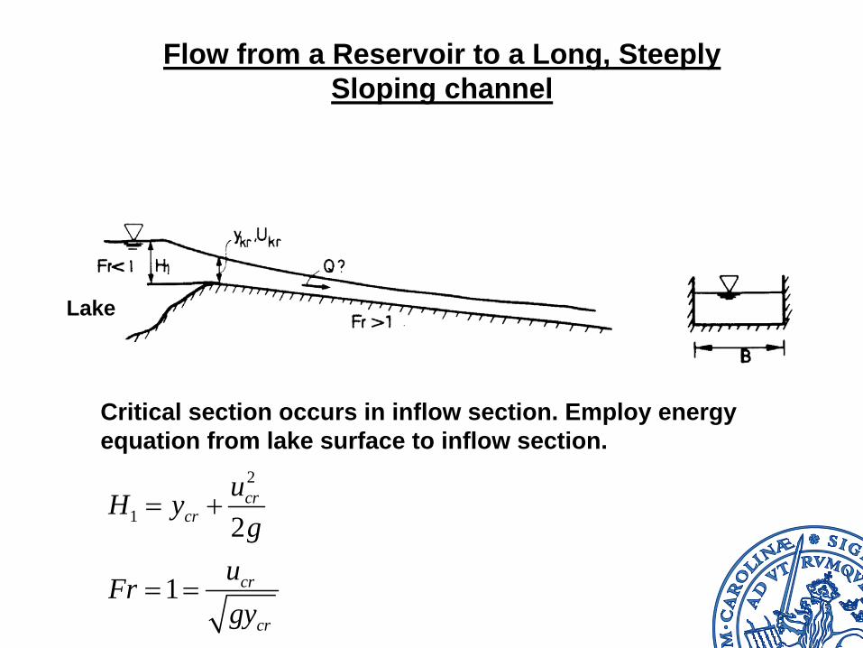
Flow from a Reservoir to a Long, Steeply Sloping channel

Critical section occurs in inflow section. Employ energy equation from lake surface to inflow section.

2

1 2

1

crcr

cr

cr

uH yg

uFrgy

= +

= =

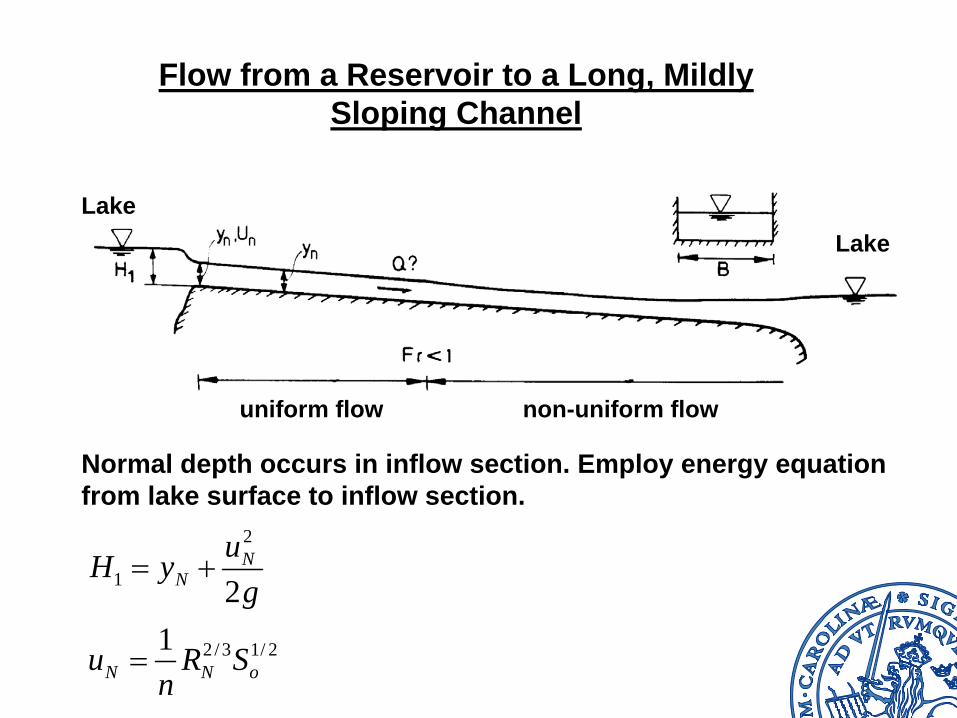
Flow from a Reservoir to a Long, Mildly Sloping Channel

uniform flow non-uniform flow

LakeLake

Normal depth occurs in inflow section. Employ energy equation from lake surface to inflow section.

2

1

2/3 1/ 2

21

NN

N N o

uH yg

u R Sn

= +

=

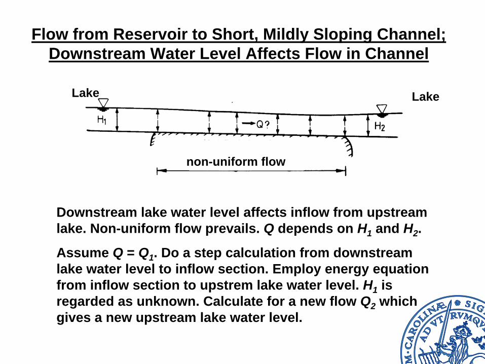
Flow from Reservoir to Short, Mildly Sloping Channel; Downstream Water Level Affects Flow in Channel

Downstream lake water level affects inflow from upstream lake. Non-uniform flow prevails. Q depends on H1 and H2 .

Assume Q = Q1 . Do a step calculation from downstream lake water level to inflow section. Employ energy equation from inflow section to upstrem lake water level. H1 is regarded as unknown. Calculate for a new flow Q2 which gives a new upstream lake water level.

Lake Lake

non-uniform flow

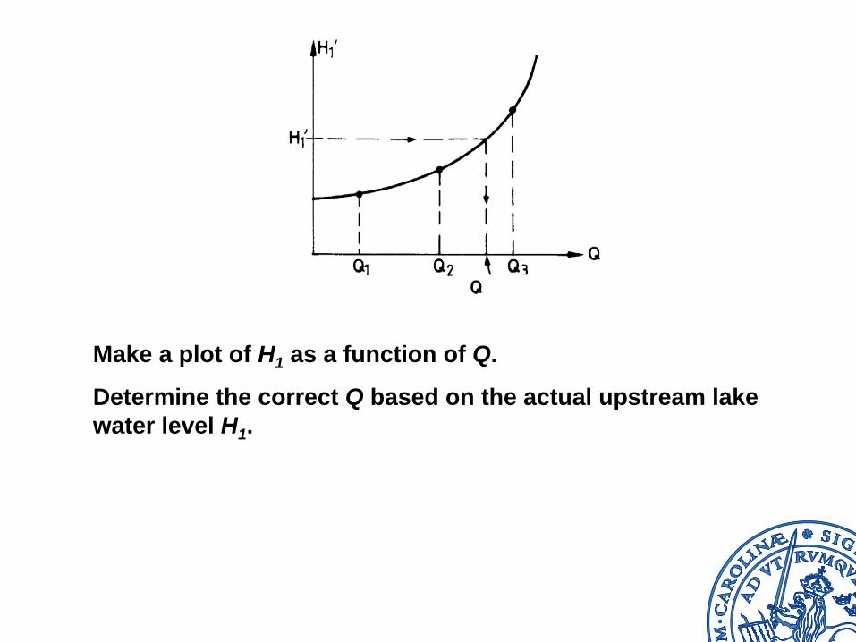
Make a plot of H1 as a function of Q.

Determine the correct Q based on the actual upstream lake water level H1 .

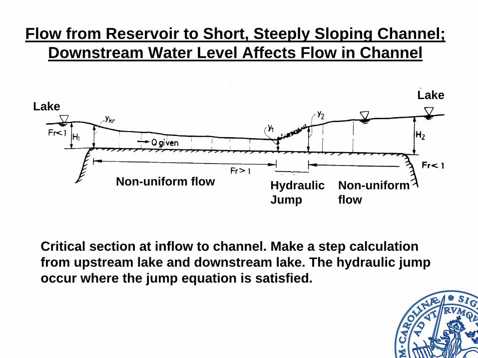
Flow from Reservoir to Short, Steeply Sloping Channel; Downstream Water Level Affects Flow in Channel

LakeLake

Non-uniform flow Hydraulic Jump

Non-uniform flow

Critical section at inflow to channel. Make a step calculation from upstream lake and downstream lake. The hydraulic jump occur where the jump equation is satisfied.

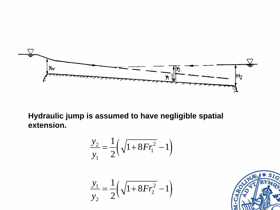
Hydraulic jump is assumed to have negligible spatial extension.

( )

( )

221

1

212

2

1 1 8 12

1 1 8 12

y Fry

y Fry

= + −

= + −