Embed Size (px)
Citation preview

Gradient polymer elution chromatography : a qualitativestudy on the prediction of retention times using cloud-points and solubility parametersStaal, W.J.
DOI:10.6100/IR458058
Published: 01/01/1996
Document VersionPublisher’s PDF, also known as Version of Record (includes final page, issue and volume numbers)
Please check the document version of this publication:
• A submitted manuscript is the author's version of the article upon submission and before peer-review. There can be important differencesbetween the submitted version and the official published version of record. People interested in the research are advised to contact theauthor for the final version of the publication, or visit the DOI to the publisher's website.• The final author version and the galley proof are versions of the publication after peer review.• The final published version features the final layout of the paper including the volume, issue and page numbers.
Link to publication
Citation for published version (APA):Staal, W. J. (1996). Gradient polymer elution chromatography : a qualitative study on the prediction of retentiontimes using cloud-points and solubility parameters Eindhoven: Technische Universiteit Eindhoven DOI:10.6100/IR458058
General rightsCopyright and moral rights for the publications made accessible in the public portal are retained by the authors and/or other copyright ownersand it is a condition of accessing publications that users recognise and abide by the legal requirements associated with these rights.
• Users may download and print one copy of any publication from the public portal for the purpose of private study or research. • You may not further distribute the material or use it for any profit-making activity or commercial gain • You may freely distribute the URL identifying the publication in the public portal ?
Take down policyIf you believe that this document breaches copyright please contact us providing details, and we will remove access to the work immediatelyand investigate your claim.
Download date: 17. Jun. 2018

Grc;.dient Polymer Elution Chromatography
A Qualitative Study on the Prediction of Retention Times using Cloud-Points and Solubility Parameters
WimJ.Staal

Gradient Polymer Elution Chromatography
A Qualitative Study on the Prediction of Retention Times using Cloud-Points and Solubility Parameters
Wim J. Staal

CIP-DAT A KONINKLIJKE BIBLIOTHEEK, DEN HAAG
Staal, Willem Jacob
Gradient Polymer Elution Chromatography: a qualitative study on the prediction of retention times using cloud~points and solubility parameters I Will em Jacob Staal.- Eindhoven: Eindhoven University of Technology Thesis Technische Universiteit Eindhoven. -With ref -With summary in Dutch. ISBN 90-386-0126-3 Subject headings: HPLC I Gradient Polymer Elution
Chromatography I polymer blends.
©Copyright Waters Chromatography B.V.

Gradient Polymer Elution Chromatography
A Qualitative Study on the Prediction of Retention Times using Cloud-Points and Solubility Parameters
PROEFSCHRIFT
ter verkrijging van de graad van doctor aan de Technische Universiteit Eindhoven, op gezag van
de Rector Magnificus, prof.dr. J.H. van Lint, voor een commissie aangewezen door het College
van Dekanen in het openbaar te verdedigen op dinsdag 12 maart 1996 om 16.00 uur
door
Willem Jacob Staal geboren te Bergen op Zoom
Drukkerij Judels en Brinkman, Delft

Dit proefschrift is goedgekeurd door de promotoren:
prof.dr.ir. AL. German en profdr.ir. C.AM.G. Cramers
Copromoter: dr. AM. van Herk
The author is indebted to Waters Chromatography the Netherlands, to the Benelux, to European Headquarters, and to the United States Headquarters at Milford Massachusetts for financially supporting this work.

in herinnering aan mijn ouders
opgedragen aan: Hanny Bastiaan Maarten
Joost-Jan

Summary
This investigation provides an outline of the results of polymer separations using High Performance Liquid Chromatography (HPLC). In spite of the fact that this technique has been used for more than ten years for the separation of copolymers (the determination of the Chemical Composition Distribution, or CCD), there is still a lack of knowledge about the various separating mechanisms of homopolymers. The aim of this investigation is to predict the most elementary separation mechanism, i.e. separation on the basis of polymer solubility. Three different model high molar mass homopolymers have been selected for use in testing this mode of separation, i.e. poly(butadiene) (PB), poly(styrene) (PS) and poly(methyl methacrylate) (PMMA). These model homopolymers serve in tum as a basis for predicting the chromatography of copolymers and terpolymers.
The chromatographic separation of polymers, based on a precipitation-redissolution mechanism, is correlated with a turbidimetric titration (precipitation) of polymers called the cloud-point test. The condition for such a correlation is that no adsorption of the dissolved polymer on the stationary phase of the chromatographic column occurs.
In order to obtain the cloud-point of a polymer solution, knowledge ofthe solubility properties of a polymer is required (Chapter 4). Therefore, the solubility properties of the selected model polymers have to be determined. The liquids used are commonly applied HPLC eluents. The results of the polymer solubility tests lead to a division of the HPLC eluents in solvents and non-solvents. A trend is observed between the polarity of the polymer and the polarity of the solvents. A joint order also of solvents and non-solvents is suggested for the three standard polymers.
Based on the division in solvents and non-solvents, the selected non-solvents are applied to perform many cloud-point titrations (Chapter 5). On the basis of these cloud-point measurements, a ranking according to a solvent and non-solvent strength is proposed.
From these cloud-point experiments the separation of the three polymers is predicted and verified by chromatographic experiments (Chapter 6). The chromatographic experiments demonstrated a good correlation between the chromatographically and titrimetrically obtained cloud-points. This result is obtained for the three different polymers, when applying different solvents and different non-solvents. Because various mechanisms are playing a role in the different steps of the chromatographic process, a new general name, viz. 'Gradient Polymer Elution Chromatography' (GPEC) is introduced.

Samenvatting
niet-oplosmiddelen. Omdat het chromatografisch proces uit vele stappen bestaat, die weer gebaseerd zijn op verschillende mechanismen, is een nieuwe meer algemene naam voor deze chromatografie ingevoerd en wei "Gradient Polymer Elution Chromatography" (GPEC).
Er is ook gepoogd de neerslagpunten te voorspellen gebruikmakend van de klassieke oplosbaarheidsparameters van Hildebrand voor vloeistoffen en de oplosbaarheidspara-meters van Hansen voor polymeren (Hoofstuk 7). De resultaten van deze voorspellingen, gebaseerd op de klassieke rekenmethode volgens de bol van Hansen, zijn slecht te noemen. Betere resultaten worden verkregen met de methode van Suh en Clarke die gebaseerd is op een vergelijking tussen de oplosbaarheidsparameter van het oplosmiddeVniet-oplosmiddel mengsel op het moment van neerslag en de oplosbaarheids-parameter van het gebruikte oplosmiddel. De meest belovende methode tot nu toe is gebaseerd op een directe correlatie tussen de neerslagpunten en de oplosbaar-heidsparameters van de toegepaste oplosmiddelen. De directe methode voldoet aan de minimum eis van de nauwkeurigheid van de voorspelde neerslagpunten waarbij een chromatografische scheiding tussen twee polymeren verwacht kan worden.
Veel gesignaleerde problemen met de HPLC scheiding van polymeren zijn ondertussen, met de kennis samengevat in dit proefschrift, al opgelost. De verkregen resultaten roepen echter ook weer vele nieuwe vragen op. Met deze overwegend verkennende en kwalitative studie naar de vloeistofchromatografische scheiding van homopolymeren, is getracht een betere basis te leggen voor het toekomstig onderzoek aan meer complexe polymeer systemen zoals copolymeren, terpolymeren en polymere blends.
Glossary of Symbols
a expansion coefficient KI p compressibility factor (MParl CED Cohesive Energy Density Jm-3
8 solubility parameter (MPa/12
Oa solubility parameter acid term (MPa)112
ob solubility parameter base term (MPa(2
0d solubility parameter dispersive term (MPa)v2
& solubility parameter hydrogen -bonding term (MPa)112
Oin solubility parameter induction term ' (MPa)I/2 omix solubility parameter of solvent mixture (MPa)I/2 ons solubility parameter of non-solvent (MPa)112
Oo solubility parameter orientation term (MPa)112
()P solubility parameter of polymer (MPa)I/2
op solubility parameter polarity term (MPa)I/2 o· solubility parameter of the solvent (MPa)I/2
81 total solubility parameter (MPa//2
AE" energy change of isothermal vaporisation J E dielectric constant Hz F group contribution of structural unit Jmor1
AG Gibbs free energy change J AH enthalpy change J e index theta state
Jl dipole moment D M molar mass gmor1
p pressure Pa p density g cm-3
RAS radius of interaction of solvent (MPa)112
RAo radius of interaction of polymer (MPa/12 R,mix radius of interaction of the solvent/non-solvent mixture at cloud-point (MPa)112
R. peak resolution AS entropy change JKI T absolute temperature K to peak elution time during the gradient min. 1L gradient lag time min. tM hold-up time of the mobile phase min. tR peak elution time mm. tsys system time mm.

v volume
volume fraction of non-solvent volume fraction of polymer volume fraction of solvent volume fraction of the solvent at the start of the gradient steepness of the gradient curve
Flory-Huggins polymer-solvent interaction parameter
Glossary of Symbols

Abbreviations
A CP CN CI8
ELSD GPC GPEC HPLC HPPLC IUPAC IR LAC NELC NMR NS PB PS PMMA s SEC Si TLC THF TMP uv
Apparent non-solvent Cloud-Point Cyano-propyl sorbent Octadecyl sorbent
Abbreviations
Evaporative Light Scattering Detection Gel Permeation Chromatography Gradient Polymer Elution Chromatography High Performance Liquid Chromatography High Performance Precipitation Liquid Chromatography International Union ofPure and Applied Chemistry Infra-Red light spectroscopy Liquid Adsorption Chromatography Non-Exclusion Liquid Chromatography Nuclear Magnetic Resonance spectroscopy Non-Solvent Poly(butadiene) Poly( styrene) Poly(methyl methacrylate) Solvent Size Exclusion Chromatography Silica sorbent Thin Layer Chromatography T etrahydrofuran 2,2, 4-Trimethylpentane Ultra-Violet light spectroscopy

Contents
CONTENTS
SUMMARY
SAMENV ATTING
GLOSSARY OF SYMBOLS
ABBREVIATIONS
CHAPTER I INTRODUCTION
1. INTRODUCTION ............................................................................................................ 1
1.1 BRIEF HISTORICAL OVERVIEW ................................................................................. 1
1.1.1 Chromatography of Polymers .................................................................................... 1 1.1.2 Choice ofPolymers .................................................................................................... 2
1.2 BACKGROUND OF THE INVESTIGATION ........................................................................... 3
1.2.1 The GPEC®Project ............................................................................................. .3 1.2.2 Polymer Separation Based on Solubility .................................................................... 3
1.3 AIM OF THE INVESTIGATION .......................................................................................... .4
1.4 OUTLINE OF THE THESIS........................... .. ........................................................ 5
1. 5 REFERENCES ................................................................................................................... 6
CHAPTER2 THEORETICAL BACKGROUND
2. THEORETICAL BACKGROUND .......................................................................................... 7
2.1 INTRODUCTION ............................................................................................................... 7 2.2 THE CHROMATOGRAPHY OF HIGH MOLAR MAss POLYMERS ....................................... 9
2.2.1 Liquid Chromatography ............................................................................................. 9 2.2.2 I socratic Analysis ....................................................................................................... 9 2.2.3 Gradient Elution...................................................... .. . .. ........................................ 1 0
2.3 TERNARY PHASE DIAGRAM ........................................................................................ 14 2.3.1 Introduction ............................................................................................................. 14 2.3.2 Influence of Polymer Fraction .................................................................................. 14 2.3 .3 Influence of Molar Mass .......................................................................................... 15 2.3.4 Influence ofTemperature ......................................................................................... 17 2.3 .5 Conclusions ............................................................................................................. 17

Contents
2.4 POLYMER-SOLVENT INTERACTION PARAMETER ......................................................... 19 2.4.1 Introduction ............................................................................................................. 19 2.4.2 The Flory-Huggins Interaction Parameter. ............................................................... 19 2.4.3 The Solubility Parameter .......................................................................................... 19 2.4.4 The Chromatogram Expressed in Solubility Parameters ............................................ 25
2.5 THE THREE VALUE SOLUBILITY PARAMETER CONCEPT .............................................. 28 2.5.1 Introduction ............................................................................................................. 28 2.5.2 The Sphere of Solubility .......................................................................................... 29 2.5.3 Mixtures of Liquids ................................................................................................. 30 2.5 .4 Calculations of Cloud-Points .................................................................................... 30
2.6 ALTERNATIVECONCEPTS ............................................................................................. 31 2.7 REFERENCES...................................................... . .................................................. 32
CHAPTER3 EXPERIMENTAL PROCEDURES
3. EXPERIMENTAL PROCEDURES .............................................................................. 35
3.11NTRODUCTION ............................................................................................................. 35 3.2 POLYMERSOLUBILITYTESTING ................................................................................... 36
3.2.1 Introduction ............................................................................................................. 36 3.2.2 Polymer Solubility Test.. .......................................................................................... 36 3.2.3 Control Test on Polymer Solubility .......................................................................... 36 3.2.4 Control Test on Polymer Insolubility ........................................................................ 37 3.2.5 Polymer Apparent Non-Solvent Test (Apparent Non-Solvent Selection) .................. 37
3.3 POLYMER CLOUD-POINT DETERMINATION .................................................................. 39 3.4 CHROMATOGRAPHICCONDITIONSFORPOLYMERSEPARATIONS ................................. 40
3.4.1 HPLC Apparatus ..................................................................................................... 40 3.4.2 Chromatographic Conditions .................................................................................. .40
CHAPTER4 SOLVENT AND NON-SOLVENT SELECTION
4. SOLVENT AND NON-SOLVENT SELECTION ....................................................... .43
4.11NTRODUCTION ............................................................................................................. 43 4.1.1 Field of Investigation ............................................................................................... 43 4.1.2 Previous Work ......................................................................................................... 43 4.1.3 Missing Information ................................................................................................. 44 4 .1. 4 Present Research ..................................................................................................... 44

Contents
4.2 RESULTS AND DISCUSSION . . . . . . . . . . . . . . . . . . . . . . . . . . . . . . . . . . . . . . . . . . . . . . . . . . . . . . . . . . . . . . . . . . . . . . . . . . ............ 46 4.2.1 Poly(butadiene) . . . . ............. .. . . . . . . . . .................................................................. .46 4.2.2 Poly(styrene) ......................................................................................................... .48 4.2.3 Poly( methyl methacrylate) ....................................... , ............................................... 50
4.3 CONCLUSIONS .................................................. , ............................................................ 53 4.4 REFERENCES ................................................................................................................. 54
CHAPTERS SOLUBILITY OF POLYMERS IN SOLVENT/NON-SOLVENT MIXTURES
5. SOLUBILITY OF POLYMERS IN SOLVENT/NON-SOLVENT MIXTURES ........ 55
5.1 INTRODUCTION ...................................................................................... , ...................... 55 5.1.1 Field of Investigation ............................................................................................... 55 5.1.2 Previous Work. ........................................................................................................ 55 5.1.3 Missing Information ................................................................................................. 56 5 .1. 4 Present Research ..................................................................................................... 56
5.1.4.1 Method ............................................................................................................. 56 5. I. 4. 2 Experimental Conditions ................................................................................... 57
5.2 RESULTS AND DISCUSSION ........................................................................... , ............... 58 5.2.1 Experimental Cloud-Point Values ofPoly(butadiene) ............................................... 58
5.2.1.1 Previous Work .................................................................................................. 58 5.2.1.2 Single Solvent Solubility Versus Solvent/Non-Solvent Solubility ...................... 58 5.2.1.3 Practical Application ......................................................................................... 65
5.2 .2 Experimental Cloud-Point Values of Poly( styrene) ................................................... 65 5.2.2.1 Previous Work .................................................................................................. 65 5.2.2.2 Single Solvent Solubility Versus Solvent/Non-Solvent Solubility ....................... 65
5. 2.3 Experimental Cloud-Point Values of Poly( methyl methacrylate) ............................... 69 5.2.3.1 Previous Work .................................................................................................. 69 5.2.3.2 Single Solvent Solubility Versus Solvent/Non-Solvent Solubility ....................... 69 5.2.3.3 Practical Application ......................................................................................... 73
5.3 CONCLUSIONS ............................................................................................................... 74 5.4 REFERENCES ................................................................................................................. 75

Contents
APPENDICES
Appendix 1: Suppliers of HPLC Solvents ......................................................................... 127 Appendix 2: Structure ofHPLC Solvents ......................................................................... 128 Appendix 3: Solubility Parameters ofHPLC Solvents ....................................................... 130 Appendix 4: Physical Properties ofHPLC Solvents ........................................................ 131 Appendix 5: Experimentally Determined Miscibility ofHPLC Solvents ............................. 132 Appendix 6: Experimentally Determined Miscibility ofHPLC Solvents ............................. 133 Appendix 7: Data ofPoly(butadiene) Standards........ ................................... .......... . ...134 Appendix 8: Data ofPoly(styrene) Standards ................................................................... 135 Appendix 9: Data ofPoly(methyl methacrylate) Standards .............................................. 136 Appendix 10: Structure ofPolymers .................................................................................. l38 Appendix 11: Published Cloud-point Values of Poly( styrene) ......................................... 138 Appendix 12: Published Cloud-point Values ofpoly(methyl methacrylate) ......................... 140 Appendix 13: Solubility Parameters of the Three Standard Polymers ................................. 141 Appendix 14: Molar Mass Dependency of the Cloud-Point at Ambient Temperature ......... 142 Appendix 15: Influence ofthe Polymer Concentration on the Cloud-Point.. ....................... l45 Appendix 16: Influence ofthe Temperature on the Cloud-Point... ...................................... 146 Appendix 17: Cloud-Points ofPoly(butadiene) Transformed in the Solubility
Parameter o::;,i• ............................................................................................. 147
Appendix 18: Cloud-Points ofPoly(styrene) Transformed in the Solubility Parameters o::;,ix and o;::,ix ........................................................................ 148
Appendix 19: The Cloud-Points of Poly( methyl methacrylate) Transformed in the Solubility Parameters o:• and o;::,ix ............................................................ l49
Appendix 20: Coefficients of omix Lines at Constant Non-Solvent using the Sub and Clarke Method ........................................................................................................ 150
Appendix 21: Coefficients ofNon-Solvent Lines of the Direct Correlation between the Cloud-Points and the Solubility Parameters of Solvents for the Three Standard Polymers ....................................................................................... 151
Appendix 22: Comparison of Observed and Calculated Cloud-Points for the Three Calculation Methods .................................................................................... 152
Appendix 23: Calculation Test based on Observed and Calculated Cloud-Points using a Combination of the Present Investigation and the Work ofSuh and Clark ............................................................................................................ 155

Introduction
1. INTRODUCTION
1.1 Brief Historical Overview
1.1.1 Chromatography of Polymers
Nowadays the type of liquid chromatography of polymers most frequently applied is Gel Permeation Chromatography (GPC), also called Size Exclusion Chromatography (SEC)[l}. This analytical separation method is based on a matching between the size distribution of the pores in the packing of the column and the size of the dissolved penetrating polymer molecules (hydrodynamic volume of the coil). The strength of this separation technique is the determination of the molar mass distribution of polymers. In the case of polymer mixtures the main problem is that most commercial thermoplastics have overlapping hydrodynamic volume distributions, meaning that all macromolecules tend to elute at the same time. In addition, most commercial products also have a broad molecular mass distribution similarly leading to a strong peak overlap in the chromatography of polymer mixtures. The result is very poor or no separation with GPC. Another restriction ofGPC is that it is relatively insensitive with respect to the determination of the chemical composition, which is often essential for understanding the properties of polymers.
For several applications it is required to characterise polymers based on differences in chemical structure. These chemical differences can be made visible by selective solubility, selective adsorption on stationary phases and by selective detectors. Traditionally, Thin Layer Chromatography (TLC) [2} and open~column chromatography [3} were applied. Another approach is a column packing coated with the polymer as a sample and eluted with an antiparallel solvent and temperature gradient. This approach is called the Baker-Williams fractionating method [4]. The separation is based on differences in redissolution behaviour of the various polymer fractions.
More recently polymers have beeh separated with High Performance Liquid Chromatography techniques (HPLC). The separations have mostly been carried out isocratically (one solvent or a constant solvent composition) or by a solvent gradient (the variation of two or more solvent compositions over a period of time).
Glockner et al. [5], Mori [6], Van Doremaele et al. [7] and Engelhardt et al. [8] used this separation method for the determination of the Chemical Composition Distribution (CCD) of copolymers.

2 Chapter 1
Researchers working on copolymers have separated the homopolymer from the copolymer (as additional information), but no systematic study has been undertaken to separate polymer mixtures or polymer blends. This thesis focuses on the separation of homopolymer mixtures.
Mori [9] performed an isocratic separation of different polymers on a silica column using different eluents. The mechanism of separation is based on a combination of adsorption and precipitation. However, this is a very time consuming and qualitative separation method for polymers.
In 1986 Mourey [10] already separated homopolymers using a solvent gradient. Jansen eta/. [11] and Staal et al. [12,13] were the first to employ a gradient HPLC separation technique specifically for polymer blends.
1.1.2 Choice of Polymers
The plastics industry nowadays is moving toward more complex polymer systems like polymer alloys, blends, composites and laminates [14]. The advantage of blends is that the desired physical properties can be adjusted over a broad range. The identification and quantification of individual components is very difficult for such complex polymer samples. Therefore, a good separation is necessary in achieving an accurate identification and quantification. Separated and collected fractions then can be identified by infrared (IR) and nuclear magnetic resonance (NMR) spectroscopy. In this thesis the separation of polymers is studied according to their solubility characteristics using liquid chromatography.
The solubility of polymers can be predicted from the solubility parameters of solvents and polymers as described by Hansen [15]. The solubility of a polymer in different solvents or solvent mixtures can be expressed as a sphere of solubility. With the Hansen solubility parameters and the sphere of solubility, the solubility of polymers in solvent/non-solvent mixtures can be predicted. With the polar and non-polar solubility parameter calculations of Suh and Clarke [16] the cloud-points (precipitation points of dissolved polymers derived from titrations with non-solvents) can be predicted. The cloud-points represent the solubility of a polymer in solvent/non-solvent mixtures.
In the present study, three polymer standards are chosen, each standard with a narrow molecular mass distribution, and differing in polymer structure and polarity. These polymers, poly(butadiene), poly(styrene) and poly(methyl methacrylate) are basic components for many polymer blends and copolymers (these three polymers do not constitute commercial blends, and therefore the term mixture will be used). Glockner [17], who has much experience in cloud-point measurements, pioneered in studying the relationship between the HPLC gradient (non-solvent/solvent composition) and the cloud-point ofthe polymer. This relationship is the subject of further investigation in the present study.

Introduction 3
1.2 Background of the Investigation
1.2.1 The GPEC® 1'Project
In 1990, Waters Chromatography BV (at that time a Division of Millipore Corporation) started a co-operation with the Laboratory of Polymer Chemistry at Eindhoven University of Technology. The aim of that co-operation was to gain a better understanding of the mechanisms governing the separation of polymers, based on a solvent gradient and performed on liquid chromatography equipment. This co-operation resulted in a project called 'Gradient Polymer Elution Chromatography' (GPEC®).
This project was started on the basis of the experience of both parties, viz. German and coworkers [18] and Staal [19), as well as on the work of Glockner (20]. The experienced problems at that time were column plugging, polymer breakthrough, non-reproducible peak shapes and peak heights. The combined expertise in polymer chemistry and chromatography at Eindhoven University and Waters Chromatography led to significant improvements.
1.2.2 Polymer Separation Based on Solubility
Early attempts by Glockner [21) proved that in the absence of specific adsorption on a stationary phase, a good relationship exists between the titrimetrically obtained cloud-point composition and eluent composition in the maximum of the chromatographic peak of a high molar mass polymer. This means that by applying titrimetrically obtained cloud-points, the chromatographic behaviour of polymers can be predicted.
Since a polymer separation based on solubility takes place according to the most dominant mechanism, the present investigation focuses on polymer solubility as a tool for predicting the chromatographic separation of polymer mixtures.
I) GPEC® is a registered tmdemark of Waters Chromatogmpby B.V.

4 1
1.3 Aim of the Investigation
The aim of the present investigation is to predict the chromatography of high molar mass polymers taking place according to a solubility mechanism. This aim can be realised by :
1.) Dividing the selected HPLC eluents in solvents and non-solvents for the chosen polymers.
2.) Application of the selected non-solvents to titrate the polymer solutions in order to determine the cloud-point composition.
3.) Determination of the correlation between the titrimetrically obtained cloud-points and the chromatographically obtained cloud-points.
4.) Prediction of the cloud-points on the basis of solubility parameters of the selected polymers, solvents and non-solvents.
In order to achieve the aim defined above. a large number of basic polymer solubility experiments have to be done in pure solvents and in mixtures of solvents and non-solvents. To obtain a good correlation between these solubility results several well-defined narrow molar mass dispersed polymer standards have to be applied.

Introduction 5
1.4 Outline of the Thesis
The various chapters in this thesis provide a contribution to the understanding of the chromatographic process of separation of the high molar mass polymers.
Chapter 2 : Theoretical Background The mechanism of separation ofhigh molar mass polymers based on a precipitation-redissolution mechanism is discussed applying ternary phase diagrams and solubility parameters.
Chapter 3 : Experimental Procedures Existing and modified experimental procedures to determine polymer solubility are presented.
Chapter 4 : Solvent and Non-Solvent Selection In this chapter the HPLC eluents are divided into solvents and non-solvents for the polymers, based on experimental observations.
Chapter 5 : Solubility of Polymers in Solvent/Non-Solvent Mixtures Based on the destinction of the HPLC eluents between solvents and non-solvents in Chapter 4, cloud-points for the three polymers studied are determined experimentally.
Chapter 6 : The Chromatography of High Molar Mass Polymers In this chapter correlations are presented between cloud-points obtained from chromatographic and titrimetric experiments.
Chapter 7 : Prediction of Cloud-Points using Solubility Parameters From the solubility parameters of the selected liquids and polymers attempts are made to predict the cloud-points and by that the retention times of polymers.

6
1.5 References
[I] Moore, J. C., J. Polymer Sci, A2, 835 (1964) [2] Tacx, J.C.J.F., German, A.L., Polymer, 30, 918, (1989) [3] Teramachi, S., Esaki, H., Polymer, 7, 593, (1975) [4] Baker, C.A., Williams, R.P.J., J. Chern. Soc. (London) 2356 (1956) [5] Glockner, G., Van den Berg, J.H.M., J. Chromatogr., 550, 629 (1991) [6] Mori, S., J. Appl. Polym.Sci. , 38, 95 (1989) [7] Van Doremaele, G.H.J., Kurja, J., Claessens, HA, German, A.L., Chromatographia,
31, 493 (1991) [8] Schultz, R., Engelhardt, H., Chromatographia, 29, 325 (1990) [9] Mori, S., J. Liq. Chromatogr., 16, I, (1993) [10] Mourey,T.H., J. Chromatogr., 357, 101(1986) [11] Jansen, J.A.J., Van den Bungelaar, J.HJ., Leenen, A.J.H, Integration of Fundamental
Polymer Science and Technology -5, edited by Lemstra, P.J., Kleintjens, L.A., 323, Elsevier, London I New York (1992)
[12] Staal, W.J., Proceedings of the International Technical Symposium on GPC and LC Analysis ofPolymers and related Materials, Waters Chromatography, Boston, Mass, U.S.A., October 1989
[13] Staal, W.J., Jansen, J.A.J., Cools, P., Van Herk, A.M., German, A.L., Proceedings of the International Technical Symposium on GPC and the Analysis ofPolymers and Additives, Waters Chromatography, San Francisco, CaL, U.S.A. (Oct. 1991)
[14] Utrack:i, L.A., Polymer Alloys and Blends, Hanser, Munich (1989) [15] Hansen, J.M.J., Paint Techno!., 39, 104 (1967) [16] Suh, K.W., Clarke, D.W., J. Polymer Sci., A-1, 5, 167 (I 967) [17] Glockner, G., Habilitationsschrift, Dresden University ofTechnology (1964) [18] Van Doremaele, G.H.J., Geerts, F.H.J.M., Van de Meulen, L.J., German, A.L.,
Polymer, 33,1512 (1992) [19] Staal, W.J., Cools,P., VanHerk, A.M., German , A.L., Chromatographia, 37,218
(1993) [20] Glockner, G., Gradient HPLC of Copolymers and Chromatographic Cross
Fractionating, Springer, Berlin (1991) [21] Glockner, G., Chromatographia, 25, 854 (1988)

Theoretical 7
2. Theoretical Background
Summary: In this chapter is treated the theoretical background of the liquid chromatographic separation of high molar mass polymers. Such a separation can be based on an adsorption and/or precipitationredissoJution mechanism. The aim of the investigation is to try to explain the precipitation-redissolution mechanism using cloud-points and solubility parameters. The chromatography is related to the titrimetrically obtained cloud-points. The cloud-points can be understood by consulting the ternary polymer/solvent/non-solvent phase diagram. The retention time in chromatography can be expressed in the more universal solvent composition and this solvent composition in turn, can be expressed in the even more universal solubility parameter.
2.1 Introduction
This chapter provides to give the theoretical background of the liquid chromatographical separation of polymers based on the precipitation-redissolution process. The different aspects to describe this process are shown in Figure 2.1.
The first aspect relates to the retention time transformed into the solvent fraction. This makes the chromatography independent of the slope of the gradient curve (Figure 2.l(A, B)).
The second aspect describes the relation between the solvent composition at elution of the polymer peak and the titrimetric cloud-point (Figure 2.l(C)). This relation was already published by Glockner ll, 2].
The third aspect consists of the influence of the polymer/solvent/non-solvent composition on the cloud-point. These influences are shown in the ternary phase diagram (Figure 2.l(D)). This phase diagram can also be applied to show the influence of temperature on the cloud-point. This subject will be discussed in Paragraph 2.3.
The fourth aspect concerns the translation of cloud-points into the more universal solubility parameter (o). Different solvent/non-solvent combinations give different cloud-points (Figure 2.l(E, F)). The cloud-points expressed in solubility parameters give comparable solubility parameter values (Figure 2.l(G)). There is no literature available in which chromatographic retention times are interpreted in terms of solubility parameters.

8
Subject
l) Retention Time
I
•
2) Solvent Composition
I
t
4) Solubility Parameter
Chromatogram
\ ©
·--- <1>1 (Solvent1)
! I
I ___ .. 0
2
I
I ---t
rR: Polymer\8
/\
- J\ Non-Solvent L-·········~···-~_\Solvent
/
3) Phase Diagram (Cioud·Point)
Figure 2.1: Schematic presentation of the different aspects of describing the theoretical background of the chromatography of polymers. The y-axis represents the intensity of the detector signal/. Fast (A) and slow (8) gradients using the same NSIS combination causing short and long retention times, (C) respectively the retention times of (A) and (B) expressed in the same solvent fraction (lP). The solvent fraction is related to the cloudpoint that is a point in the phase diagram (D). Different cloud-points give different polymer peak positions {E, F), but expressed in the solubility parameter it is a comparable peak position (G).

Theoretical Background 9
2.2 The Chromatography of High Molar Mass Polymers
2.2.1 Liquid Chromatography
Liquid chromatography is an analytical separation technique. The definition of the general term chromatography formulated by the International Union of Pure and Applied Chemistry (IUPAC) is as follows: "Chromatography is a physical method of separation in which the components to he separated are distributed beh1!een h1!o phases, one of which is stationary (stationary phase) while the other (the mobile phase) moves in a definite direction "[7). The IUPAC definition of the more specific term liquid chromatography is as follows: "A separation technique in which the mobile phase is a liquid Liquid chromatography can he carried out either in a column or on a plane "[7]. Liquid chromatography can be divided, according to the mobile phase composition, in two groups of applications, i.e. isocratic analysis and gradient analysis.
2.2.2 !socratic Analysis
The IUPAC definition of isocratic analysis is as follows: "The procedure in which the composition of the mobile phase remains constant during the elution process [7)". This process usually works well for small molecules, which are distributed between the mobile and the stationary phase. Increased adsorption of the solute onto the stationary phase results in longer retention times. Such a strong adsorption of the solute can be caused by a very attractive stationary phase or a weak eluent
For high molar mass polymers, however, the situation with respect to the adsorption on the stationary phase and the solubility in the mobile phase is completely different When a polymer is dissolved most solvents are so strong that adsorption of the polymer onto the stationary phase is an exception.
Complex mixtures of high molar mass polymers are hard to separate by isocratic procedures. Applying SEC/GPC, a large difference in the hydrodynamic volume must be present to obtain a good separation [2). Most commercial high molar mass polymers, however, have comparable hydrodynamic volumes.
Another isocratic procedure for polymers is critical chromatography [3]. The influence of the molar mass on the retention time in size exclusion chromatography, is opposite to that in adsorption chromatography. At the so-called 'critical point' (solvent/non-solvent composition) both interactions are in balance and the retention time of the polymer is independent of the molar mass. Each polymer has its own characteristic critical point. At high molar mass however, the polymer in some cases is already precipitated before reaching the critical point. For many reasons this isocratic procedure is not very practical for the separation of complex mixtures of high molar mass polymers.

10 2
The separation of complex mixtures of high molar mass polymers by isocratic adsorption procedures [4, 5] is not attractive either. First, only a very few high molar mass polymersolvent combinations give adsorption on stationary phases. Second, when adsorption occurs for one of the polymers from the mixture, it is likely that the other polymers will either have no adsorption, or a too strong adsorption, or will not even be soluble in the selected solvent. This means that in nearly all cases a solvent gradient is required ..
An isocratic separation can be performed also on a solubility mechanism. However, for complex mixtures of high molar mass polymers this is not very attractive. For example, the titration curve of a high molar mass polymer solution and a non-solvent is very steep (6]. This means that the transition area between soluble and insoluble is very narrow. In a region of 0. 1-0.5% non-solvent extra, the high molar mass polymer moves from a short retention time to infinite retention time. For this reason this isocratic elution procedure is called by Mori the "on-off" elution method (2, 5]. Each polymer has its own region of solubility. This makes that applying a solvent gradient is the most practical approach for the separation of a mixture of high molar mass polymers.
An interesting approach is the combination of isocratic techniques. Balke and Patel (35] separated polymer mixtures using a para! ell (orthogonal) coupling of different SEC/GPC columns or a combination of adsorption and SEC/GPC columns. Very interesting work has been done by Janco, Berek and Prudskova [36] using an on-line combination of adsorption and SEC/GPC columns. These methods also need more time to find the right separation conditions than a gradient method.
2.2.3 Gradient Elution
For gradient elution the IUPAC definition is as follows: "The procedure in which the composition of the mobile phase is changed continuously or stepwise during the elution process" [7]. In a specific form of gradient elution of high molar mass polymers, the chromatography starts with the flow of a non-solvent through the column (Figure 2.2). In this example a mixture of two dissolved polymers is injected in the non-solvent. The two polymers are precipitated in the non-solvent and retained on the head of the column (Figure 2.2(A)). Simultaneously the solvent gradient starts by adding a good solvent in increasing amounts to the non-solvent. Each polymer redissolves during the solvent gradient at an eluent composition that depends on its molar mass and chemical structure [1]. If the eluent strength of the mobile phase is sufficiently strong to exclude adsorption of the polymer on the stationary phase, the polymers are eluted in a solvent/non-solvent composition corresponding to their cloud-point. This cloud-point represents the solvent/non-solvent composition at which the first turbidity occurs (2] during the titration of a polymer solution with the non-solvent. As shown in Figure 2.2 (B) during the gradient the first polymer redissolves at a low solvent fraction and the second polymer redissolves at a high solvent fraction (Figure 2.2 (C)). As a consequence polymers can be separated based on differences in solubility.

Gradient Profile
®! ! 100% Solvent
©
@ Column
-{a F~ ---~ --- ~ __ t;J____ _] ___ _..,. I I I I r
0% Solvent
(j) ____ ~-·rr·--F::r~~ .....
-+j__ __ ~_c2__~ I I I I I I I
II
Figure 2.2 : Schematic presentation of the precipitation-redissolution process. (A) Injection of the polymer solution in the eluent (non-solvent) and precipitation of a mixture of two polymers at the head of the column. (B) Redissoluting and eluting of the first polymer from the column at the beginning of the gradient cuNe. (C) Redissoluting and eluting of the second polymer in a stronger eluent near the end of the gradient cuNe.

12
A
I I
2
e R
time Figure 2.3: Schematic presentation of a non-solvent/solvent gradient chromatogram expressed in chromatographical terms. The y-axis represents the intensity of the detector signal I and the x-axis represents the analysis time. The two peaks are the unretained injection solvent peak (h) and the eluted polymer peak (i). The polymer peak i is positioned on the non/solvent-solvent gradient curve and eluted at solvent composition <~>:. The gradient starts at solvent composition <I>~ and the slope of the gradient is expressed in <~>:. The time between start (injection) and solvent peak (h) is the hold-up time (tM) of the mobile phase in the column. The hold-up time of the mobile phase from gradient mixer to the column inlet is called the lag time (tJ. The sum of both times is called the system time (lsys). The sum of the system time and the gradient time is the peak retention time of polymer i (t~ ).
In Figure 2.3 a chromatogram is shown of polymer i eluting at the gradient retention time t~. This retention time can be expressed in the volume fraction of the solvent ( <~>!) for polymer i.
where
(2.1)
<I>~ elution volume fraction of the solvent for polymer i
<I>~ = volume fraction of the solvent at the beginning of the gradient
<I>~= d<l>s =the increase in solvent composition (<1>5 ) with time or slope of dt
the gradient curve

where t~ = the peak retention time of polymer i during the gradient
For a linear gradient Equation 2.1 can be written as:
(2.2)
If the gradient starts with 100% non-solvent the tenn <~>: is zero. The slope of the gradient curve influences the dissolution rate and consequently the analysis time.
The peak elution time t~ of the whole analysis includes two additional parameters besides
t~. The first parameter is the hold-up time of the mobile phase in the column, and the second parameter is the lag time or time required for the mobile phase to move from the gradient mixer to the column inlet. These are two system constants.
(2.3)
where t~ = peak retention time of polymer i tL = lag time, time required for the mobile phase to move from gradient
mixer to column inlet tM = hold-up time of the mobile phase in the column
In practice the hold-up time in the column and the gradient lag time are expressed in the system time (t,ys)
t,ys tL +tM (2.4)
t~ t,ys + t~ (2.5)
The combination of Eq. 2.2 and 2.5 gives:
(2.6)
Because <1>;, <I>~ and tsys are fixed by experimental conditions, the peak retention time of polymer i is directly related to the solvent composition <1>~. As shown in the Figures 2.1 E and F the peak retention times can now be expressed in the more universal solvent composition ( <1>~). As pioneered by Glockner [1 ], the solvent composition at elution of the polymer peak from the column can be correlated to titrimetrically obtained cloud-points. Factors that influence the cloud-point composition are related to the polymer/solvent/nonsolvent ternary phase diagram as will be discussed in the next section.

14 2
2.3 Ternary Phase Diagram
2.3.1 Introduction
As already explained the retention time for the chromatography of high molar mass polymers is often based on a precipitation-redissolution mechanism. Such a mechanism can be correlated to titrimetrically observed cloud-points. The theoretical background of these cloud-points can be explained by the polymer/solvent/non-solvent ternary phase diagram (Figure 2.4). The factors of influence on the phase diagram are: the composition (polymer, solvent and non-solvent), the molar mass of the polymer and temperature.
2.3.2 Influence of the Polymer Fraction
An example of a ternary phase diagram is shown in Figure 2.4. The polymer is completely soluble in the solvent and is completely or partially insoluble in the non-solvent. The solvent and the non-solvent are completely miscible. The shaded area Figure 2.4(1) denotes the region of partial miscibility of the polymer in mixtures of the applied solvent and nonsolvent. The line around the shaded area illustrates the transition between solubility and insolubility or the cloud-points.
The amount of polymer, solvent and non-solvent is expressed in volume fractions. The cloud-point is defined as the volume fraction of the non-solvent.
CP yns <I>""
100 VP+V'+Vos (2.7)
For all co-ordinates in the phase diagram, the sum of all volume fractions equals unity.
(2.8)
In this investigation the polymer volume was 102-103 times smaller than the solvent and non-solvent volume. For this reason the polymer volume was neglected in all cloud-point calculations in this investigation.
This does not mean that the polymer fraction is not important. As shown in Figure 2.4 the polymer fraction can have a dramatic influence on the cloud-point.

Theoretical 15
<1> (polymer) p
0 LLd:~:=:~:~~=~~==••~~(~ 1
<l>ns (Non-Solvent)
Figure 2.4: Illustration of a polymer, solvent and non-solvent ternary phase diagram. The shaded area (1) illustrates the region of partial miscibility. Une (2) illustrates the transition between complete miscibility and partial miscibility. Une (3) illustrates the constant polymer fraction line for different solvent/non-solvent fractions. Point (4) represents the co-ordinates of a cloud-point of interest.
2.3.3 Influence of Molar Mass
The cloud-point not only depends on the composition of the ternary system, but also on the molar mass of the polymer (see Figure 2.5 (A)). At decreasing molar mass the polymer becomes soluble at a larger fraction of non-solvent (See Appendix 14).
A large difference in the influence of the polymer fraction on the cloud-point between low and high molar mass polymers is illustrated in Figures 2.5(A) and (B). In Figure 2.5(A), two ternary phase diagrams are shown for three polymers e.g.(l),(2) and (3) with increasing molar mass. The intersection with the constant polymer fraction line ( 4) gives the cloud-points (5), (6) and (7). Increasing the polymer fraction as illustrated in Figure 2.5 (B), results in a dramatic effect on the cloud-points (5) and (6) of the low and medium molar mass polymers. This does not apply to extremely low concentrations (Figure 2.5 is only an illustration), because the cloud-point is hardly affected by the polymer fraction (censtant cloud-point line) for high molar mass polymers. For the chromatography this

16 2
means that the retention times of low molar mass polymers may be strongly influenced by the polymer fraction. This phenomenon was reported by Glockner [1]. The unique property of high molar mass homodisperse polymers is that the cloud-point is only slightly affected by the polymer fraction (see also Appendix 15).
@)
Figure 2.5: Schematic presentation of the influence of the molar mass on the ternary phase diagram (A). Curve (1) represents an oligomer, curve (2) a medium molar mass polymer and curve (3) a high molar mass polymer. Line (4) illustrates a constant polymer fraction. The points (5), (6) and (7) illustrate the cloud-points corresponding to the intersection with the polymer fraction line (4). Figure (B) illustrates the influence of a larger polymer fraction (4) on the cloud-points (5), (6) and (7).

Theoretical 17
2.3.4 Influence of Temperature
The temperature also has a strong influence on the solubility behaviour of the polymer in the ternary phase diagram. In Figure 2.6 a three-dimensional presentation is shown of the influence of the temperature on a low (I) and high molar mass polymer (2) in the ternary phase diagram. At increasing temperature the non-solvent even becomes a solvent for the polymer.
For the chromatography of polymers based on a precipitation-redissolution mechanism, it is important to start with a proper precipitation mechanism, i.e. at a large fraction of nonsolvent deep in the ternary phase diagram.
There is an important difference in the effect of the temperature on the cloud-point of low and high molar mass polymers. As shown in Appendix 16, the cloud-point of low molar mass polymers is strongly affected by the temperature and the cloud-point of high molar mass polymers is less affected by the temperature. These results are presented in Figure 2.6 where the low molar mass polymer reaches the point of complete solubility in the nonsolvent at a smaller temperature increase than the high molar mass polymer.
The effect of the temperature on the chromatography is that at a varying column temperature the largest variations in retention times can be expected for low molar mass polymers. In general the temperature can also be applied to separate polymers based on selective solubility [30]. Because of the large differences in temperature needed for such a separation, problems related to the boiling point and freezing point of the liquids will occur. This and a lot of other reasons make a temperature gradient unattractive for a routine separation of high molar mass polymers.
2.3.5 Conclusions
To understand the effect of the composition (polymer, solvent and non-solvent), molar mass and temperature on the cloud-point, it is advisable to consult the ternary phase diagram of such a system. For high molar mass polymers, the cloud-point under chromatographic conditions is usually not much influenced by the polymer fraction, molar mass and temperature.

18
Temperature
~
2
Figure 2.6: Schematic presentation of the influence of the temperature on a low molar mass polymer(1) and a high molar mass polymer (2) in the ternary phase diagram.
Theoretical 19
2.4 Polymer-Solvent Interaction Parameter
2.4.1 Introduction
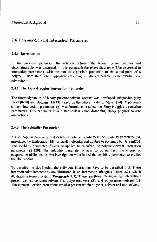
In the previous paragraph the relation between the ternary phase diagram and chromatography was discussed. In this paragraph the phase diagram will be expressed in interaction parameters, with the aim to a possible prediction of the cloud-point of a polymer. There are different approaches resulting in different parameters to describe these interactions.
2.4.2 The Flory-Huggins Interaction Parameter
The thermodynamics of binary polymer-solvent systems was developed independently by Flory [8-10] and Huggins [11-13], based on the lattice model of Meyer [14]. A polymersolvent interaction parameter (X) was introduced (called the Flory-Huggins interaction parameter). This parameter is a dimensionless value describing binary polymer-solvent interactions.
2.4.3 The Solubility Parameter
A very popular parameter that describes polymer solubility is the solubility parameter (o), introduced by Hildebrand [15] for small molecules and applied to polymers by Hansen[23). The solubility parameter (o) can be applied to calculate the polymer-solvent interaction parameter (X) [20]. The solubility parameter is easy to obtain from the energy of evaporation of liquids. In this investigation we selected the solubility parameter to predict the cloud-point.
To describe the cloud-point, the individual interactions have to be described first. These intermolecular interactions are illustrated in an interaction triangle (Figure 2. 7), which illustrates a ternary system (Paragraph 2.3). There are three intermolecular interactions present i.e., solvent/non-solvent (1), polymer/solvent (2), and polymer/non-solvent (3). These intermolecular interactions are also present within polymer, solvent and non-solvent.

20 Chapter 2
Polymer
~-.----------.-Non-Solvent CD Solvent
Figure 2. 7: 1//ustration of the interactions between, solvent/non-solvent (1 ), polyrnersolvent (2) and polymer/non-solvent (3).
In the case of mixing between solvent (S) and non-solvent molecules (NS) it is assumed that first this intermolecular interactions between solvent molecules and non-solvent molecules have to be overcome, before a new solvent/non-solvent interaction (S-NS) will be formed.
(S- S)+(NS- NS) ~ 2(S- NS) (2.9)
Such a spontaneous mixing process is governed by the Gibbs free energy of mixing. The free energy change of mixing can be divided into enthalpie (MI) and entropie (AS) contributions. The enthalpie contribution stands for the attractive or cohesive forces between molecules. The entropie contribution is related to the number of possible arrangements of the molecules in the liquid mixture.
where AGmix = the Gibbs free energy change on mixing [J] ~ix = the enthalpy change on mixing [J] LiSmix = the entropy change on mixing [J K 1
]
T = the absolute temperature [K]
(2.10)

Theoretica! Background 21
The condition necessary for a spontaneous mixing process is that the free energy change u pon mixing must be negative and the shape of the curvature must be uniformly positive. Examples of such curves are shown in Figure 2.8. The largest entropy of mixing is obtained when two small molecule liquids which are soluble in each other are mixed Fig. 2.8 (A). The entropy of mixing of a polymer and a low molar mass solvent is less than for two low molar mass solvents. This means that the minimum Gibbs free energy change during mixing is at a higher level (Figure 2.8. B). During mixing of a polymer and a poor solvent a plait in the curve may appear, which indicate~the presence ofphase separation. In Figure 2.8. D an illustration of a demixing curve of a polymer with a non-solvent is shown (real curves are more asymmetrical).
®
--------- ·-- __ !. _____________ _
0 (Solvent)
0.5 <I>--~
1 (Polymer)
Figure 2.8: Graphical il/ustration of the tree energy during mixing (L1~x ) versus the solvent-polymer composition for (A) solvent- vel}' low molar ma ss polymer, (B) polymerstrong solvent, (C) polymer - poor solvent (local demixing) and (D) polymer/non-solvent (complete demixing).

22
0
I I I
J I I I I ---,
0
(Solvent)
I
0.5 <1> ---~
l
(Polymer)
Chapter 2
Figure 2.9: Graphical illustration of the effect of demixing of a polymer on the free energy of mixing (Ll~x) curve (A) and the temperafure - polymer - solvent equilibrium phase diagram (B).
Figure (A) illustrates the free ener!,>y on mixing (f!Gmix) versus the polymer-solvent fraction at two different temperatures. These temperatures are selected from the temperature versus the polymer-solvent fraction ternary phase diagram (Figure B). T1 represents a demixed polymer-solvent phase and T2 represents a completely miscible polymer-solvent phase.
The conneetion between the .1Gmix curve and the temperature-polymer -solvent phase diagram is shown in l<'igure 2.9. The plait in the f!Gmix curve corresponds to the region of partial miscibility of the polymer. At increasing temperatures the plait becomes smaller and it disappears at the Upper Critica/ Salution Temperature (UCST). This is the maximum temperature at which the system begins to separate in two phases.

Theoretical Background 23
The interaction energy between molecules can be expressed in a numerical value. For pure low molar mass liquids like the solvent and non-solvent, the interaction energy between molecules can be determined by the energy change of evaporation t:\Ev. This energy change is defined as the energy upon isothermal vaporisation of the saturated liquid to the ideal gas state at infinite volume. This energy can be determined calorimetrically. The energy of
vaporisation per unit volume is called the Cohesive Energy Density (CED) = ( ~v)
Hildebrand [15] defined the solubility parameter (6) as the square root of the cohesive energy density.
(2.11)
where 5; = solubility parameter of species i [J.m·3f12
t:\E~ energy change upon isothermal evaporization of species i [J] Vi molar volume of species i [ m3
]
The solubility parameter is the net result of interactions like Van der Waals, dipole and hydrogen bonding forces. The dimensions of the solubility parameter (S) are (caVcm3
)1/2 =
2.046x10³ (J/m3)
112 = 2.046 (MPa)1
/2 and can be considered a measure for the 'internal
pressure' of the liquid.
The heat of mixing(~, Eq 2.10) can be approximated in terms of solubility parameters. For a mixture of a solvent and a non-solvent this is:
(2.12)
where solubility parameter of the solvent [J.m·3t 2
= solubility parameter of the non-solvent [J.m-3]
112
= the volume ofthe solvent/non-solvent mixture [m3]
The combination ofEq. 2.10 with Eq. 2.12 gives:
(2.13)
For the liquids to be miscible AH-T t:\S must be negative. The term Vmix ( 5' om r <I>'<P""

24
is always positive. The lowest or minimum value for this term is reached when o· -ODS is zero or when the solubility parameters have the same value. This is the case when the components have the same basic structure. The basic rule of thumb for solubility is 'like dissolves like' (' simi/ia simi/ius so/vuntur ').
2
Most low molar mass liquids, however, are miscible as shown in Appendices 5 and 6. Low molar mass liquids have a high entropy causing good miscibility as shown in F'igure 2.8. If the difference in solubility parameter, however, is too large, partial or complete immiscibility occurs.
The solubility parameter of a polymer, however, cannot be determined from the energy of vaporisation directly, because the polymer will decompose before reaching its boiling point. However, the solubility parameter of the polymer can be obtained from the volume expansion coefficient (a.) and the compressibility factor (/J) [26], according to:
(2.14)
where T = absolute temperature [K] a= isobaric expansion coefficient [K1
]
P= isothermal compressibility factor [MPar1
Many tests have been developed to indirectly determine the solubility parameter of a polymer via solvency testing [19], the maximum swelling [20) of a cross-linked polymer, maximum intrinsic viscosity [21], and cloud-point testing [22].
An estimation of the solubility parameter of a polymer can be calculated from group contributions such as those performed by Small [16], Hoy [17] and Van Krevelen and Hoftyzer [18]. Small's method is presented in Equation 2.15.
where P; = the density of polymer i [Kg.m-3)
M; = molar mass of polymer i [g.mor1]
(2.15)
Fj.i =contribution of structural unit j and i(sum of group contributions) [lmor1)
To describe the solubility of a polymer in a solvent/non-solvent mixture, the polymersolvent and the polymer/non-solvent interactions have to be known (Figure 2. 7). An easier way to describe the polymer solubility is to combine the solubility parameter of solvent and non-solvent to a new average value. This method is based on the assumption that the solvent/non-solvent mixture at cloud-point conditions can be assumed to be a new solvent

25
with its own solubility parameter. Hildebrand 115] called this solubility parameter of
mixtures of solvents the effective solubility parameter (8). Barton [23] applied this
effective solubility parameter for calculations of the solubility of polymers. This work was
based on the single liquid approach of mixtures of liquids by Scott L24,25J.
<l>s + <J>"s (2.16)
and
(2.17)
The conditions for such an approach are that the solvent and non-solvent must be miscible
and no volume change during mixing (contraction) may occur.
Instead of the name effective Hildebrand parameter, Suh and Clarke [22] suggested the name solubility parameter of the solvent/non-solvent mixture (omix) at cloud-point conditions. This name is more related to the application. In this investigation the notation omix will be applied.
(2.18)
Once the solubility parameter of the polymer has been determined, the Gibbs free energy for the polymer-solvent and polymer/non-solvent can be obtained.
(2.19)
where V "" total volume of polymer, solvent and non-solvent mixture
As shown in Figure 2.4 the polymer fraction ( <PP) can have a large influence on the polymer solubility. Now the ternary diagram of Figure 2.6 changes into a binary diagram as shown in Figure 2.9. From Eq 2.19, the AGmix curve can be obtained.
2.4.4 The Chromatogram Expressed iu Solubility Parameters
As suggested by Suh and Clarke [22] Equation 2.18 can be written as:
or <t>• (2.20)

26 2
100% Solvent( I) cr; 1 000/o Solvent(2)
1 000/o Solvent
Figure 2.10: Graphical illustration of gradient chromatograms of the same polymer in different non-polar solvent/non-solvent mixtures. The y-axis represents the intensity of the detector signal/ and the x-axis represents the fraction solvent during the gradient. In chromatogram (A) the polymer (1) is eluting at a low fraction solvent. In chromatogram (B) the same polymer (2) is eluting at a high fraction solvent in another solvent/nonsolvent (non-polar) combination. If both gradient curves are expressed in solubility parameters both peaks have a comparable o;:;
Now the cloud-point is expressed in terms of solubility parameters. The combination of Equation 2.6 and Equation 2.20 gives the retention time of the chromatography expressed in the more universal solubility parameters.
(2.21)
The retention time can be directly calculated from the solubility parameter of the solvent(o"), non-solvent (ons) and the solubility parameter of the cloud-point (omix)
The expression 'more universal' means that early (Figure 5.10 (A)) and late (Figure 2.10 (B)) eluting peaks give comparable peak positions in the chromatogram expressed in solubility parameters (Figure 2.10 (C)).
I
I ()mix
np
27
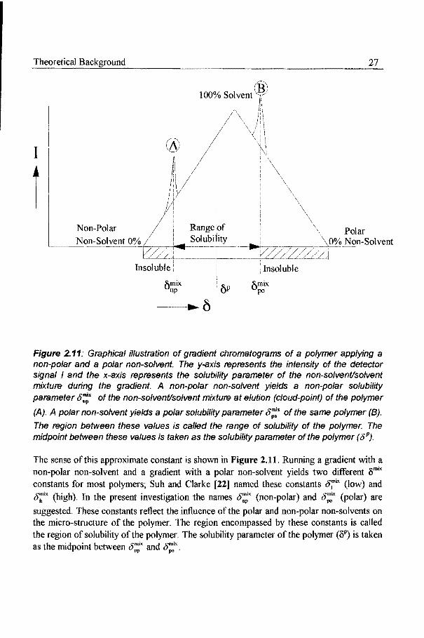
Figure 2.11: Graphical illustration of gradient chromatograms of a polymer applying a non-polar and a polar non-solvent. The y-axis represents the intensity of the detector signal I and the x-axis represents the solubility parameter of the non-so/vent/solvent mixture during the gradient. A non-polar non-solvent yields a non-polar solubility parameter &~;x of the non-solvent/solvent mixture at elution (cloud-point) of the polymer
(A). A polar non-solvent yields a polar solubility parameter&;~· of the same polymer (B).
The region between these values is called the range of solubility of the polymer. The midpoint between these values is taken as the solubility parameter of the polymer ( oP).
The sense of this approximate constant is shown in Figure 2.11. Running a gradient with a non-polar non-solvent and a gradient with a polar non-solvent yields two different smix
constants for most polymers; Suh and Clarke [22] named these constants t5~ix (low) and 8;:"" (high). In the present investigation the names &:~"' (non-polar) and ~ (polar) are
suggested. These constants reflect the influence of the polar and non-polar non-solvents on the micro-structure of the polymer. The region encompassed by these constants is called the region of solubility of the polymer. The solubility parameter of the polymer (oP) is taken as the midpoint between &:X and &::X.

28 2
2.5 The Three Value Solubility Parameter Concept
2.5.1 Introduction
In addition to the single value solubility parameter approach, a three value solubility parameter approach was proposed by Hansen and Skaarup [26]. The basis of this three value solubility parameter concept is the assumption that the total cohesive energy E can be divided into contributions from dispersive forces (Ed), permanent dipole - permanent dipole forces (Ep) and hydrogen bonding forces (Eh).
Dividing this equation by the molar volume of a solvent V gives:
Combination with Eq. 2.11 gives:
where od =dispersive term [MPat2
ov =polar term [MPa] 112
Oh =hydrogen bonding term [MPa]112
(2.22)
(2.23)
(2.24)
The dispersive term Sd (London interaction) can be obtained from the refractive index values presented by Koenhen and Smolders [27]. The polar term SP, can be related to the dielectric constant (&) and the dipole moment (J.l), as presented by Hansen and Skaarup [26]. Hansen and Beerbower [28] calculated hydrogen bonding terms oh for many solvents. These individual solubility parameters can also be calculated from group contributions [16-18].

29
2.5.2 The Sphere of Solubility
The polymer solubility is maximal if the solubility parameters of solvent and polymer are equal. The tolerance in the solubility parameters between solvent and polymer are expressed in the so-called radius of interaction of the solvent, R~ [23].
R: [4(o~ ~o:f +(o~ ~s:r +(o: o~fr (2.25)
where radius of interaction of the solvent [MPa] 112
dispersive term of the solvent [MPa] 112
dispersive term of the polymer [MPa]112
hydrogen bonding term of the solvent [MPa]112
= hydrogen bonding term of the polymer [MPa] 112
op• polar term of the solvent [MPa] 112
o/ = polar term ofthe polymer [MPa] 112
The three solubility parameter values of the polymer can be collectively presented as a coordinate in a three-dimensional plot (Hansen [26]) (Figure 2.12). By doubling the 0d-axis (scaling factor) the co-ordinates of the solubility parameters of the solvents for a polymer result in a spherically shaped cloud around the co-ordinate of the solubility parameters of the polymer. The radius of this sphere R~o is called the radius of interaction of the polymer starting in the centre of the sphere at the co-ordinate of the polymer. This radius is an empirical value determined by the best fitting radius in the cloud of observed solvents l28). Non-solvents are located outside the sphere and the solvents are located inside the sphere.
Figure 2.12: Schematic presentation of the sphere of solubility. The radius of interaction of the solvent (Rl) is located inside the sphere and the radius of interaction of the nonsolvent is located outside the sphere.

30
2.5.3 Mixtures of Liquids
Calculations or predictions of polymer solubility with the three value parameter model can be extended to many component systems. In analogy with the single liquid approximation used for the single value solubility parameter approach, the mixture is assumed to be a linear combination of the partial contributions of the individual solubility parameters.
For a binary mixture of liquids (solvent and non-solvent) the solubility parameters of the mixture are based on Eq. 2.18:
(2.26)
(2.27)
(2.28)
where volume fraction of solvent <l>ns volume fraction of non-solvent
Combination of Equations 2.26, 2.27, 2.28 with Equation 2.29 gives the radius of interaction of the solvent mixture RA mix
R~« = [4(8:" -8:f +(8;m 8~r +(8;:"' -8:n112
(2.29)
or
R:ix =[ 4((<t>"o~ +<I>nsa:;s)-a:r +((<t>"o; +<I>nsa;)-a~r +((<t>·o~ +<I>nsa;:s) a:rT (2.30)
2.5.4 Calculations of Cloud-Points
In this thesis the Hansen multi-solvent solubility parameter calculations were applied to calculate cloud-point values directly. The basis of these calculations is that the shell of the sphere of solubility is determined by the transition from polymer solubility to insolubility, or the cloud-point area. The addition of non-solvent to a solvent, moves the solvent coordinate of the mixture towards the shell of the sphere. Outside the shell the polymer is insoluble. On the shell of the sphere (the cloud-point) the radius of interaction of the solvent/non-solvent mixture (RA mix) is equivalent to the radius of interaction of the polymer (RAoP). At this outer boundary of the sphere, the volume fraction of the non-solvent (<l>ns) is the unknown parameter. With Eq 2.30 the cloud-point composition can now be calculated.

Theoretical 31
2.6 Alternative Concepts
In general much is still unknown about the interactions between molecules in a liquid. A large number of physical parameters can be determined. Many of these parameters depend on each other. Many concepts have been formulated to obtain the coherence between the individual parameters. Many investigators have broken up the Hildebrand solubility parameter(15J into several terms. For example in the five parameters model (Table 2.1) the polarity term is split up into an orientation and an induction term. The hydrogen-bonding term can be split up into an acid and a base term. The four and five parameter equations are applied in adsorption and partition chromatography to calculate the retention time [33].
Table 2.1: Overview of Formulas to Calculate the Total Solubility Parameter (6t)
81 Single value parameter approach (23]
82 = 32 +32 I d p (2.3]) Two value parameter approach [31)
32 =02 +32 +·32 t d p b (2.24) Three value parameter approach [32]
8! +o! +28,ob (2.32) Four value parameter approach (33)
(2.33) Five value parameter approach [34]
where 3,,2 = 28a3b [MPa] Op2
= 3<>2 + 2(hn3d [MPa] Oo orientation term (dipole-dipole) [MPa] 112
Oin induction term (induced dipole) [MPa] 112
Oa acid term (proton donor) [MPa]"2
Ob base term (proton acceptor) [MPa] 112
Even complex formulas like Equation 2.33, cannot be applied to water or strong hydrogen bonding solvents. The present models allows for first order predictions. From the first order predictions, corrections have to be made based on observations [29]. Most values in the four and five parameter concepts are not available for polymers.

32 Chapter 2
2. 7 References
[1] Glockner, G.,Chromatographia, 25, 854 (1988) [2] Glockner, G., Polymer Characterisation by Liquid Chromatography, Elsevier,
Amsterdam, (1987) [3] Cools, P.J.C.H., Van Herk, A.M., German, A.L., Staal, W.J., J. Liq. Chromatogr.,
17,3133 (1994) [4] Scheutjens, J.M.H.M., Fleer, G.J., J.Phys.Chem., 83, 1619 (1979) [5] Mori, S., J. Liq. Chromatogr., 16, 1 (1993) [6] Elias, H-G., Tung, L.H., Fractionation of Synthetic Polymers, Dekker, New York
(1977) [7] Ettere, L.S., Pure Appl. Chern., 65, 819 (1993) [8] Flory, P.J., J.Chem.Phys., 10, 51 (1942) [9] Flory, P.J., J.Chem.Phys., 12,425 (1944) [10] Flory, P.J., Principles of Polymer Chemistry, Cornell University Press, Ithaca
(1953) [11] Huggins, M.L., J. Phys. Chern., 46, 151 (1942) [12] Huggins, M.L., J. Am. Chern. Soc., 64, 1712 (1942) [13] Huggins, M.L., Physical Chemistry ofHigh Polymers, Wiley, New York (1958) [14] Meyer, K.H., Z. Phys. Chern., B44, 383 (1934) [15] Hildebrand, J.H.,J. Am. Chern. Soc., 38, 1452 (1916) [16] Small, P.A., J. Appl. Chern., 3, 71 (1953) [17] Hoy, K.L., J. Paint Techno!., 42, 76, (1970) [18] Van Krevelen, D.W., Hoftyzer, P.J., J. Appl. Polym. Sci., 11, 2189 (1967) [19] Gee, G., Trans. lnst. Rubber Ind., 18, 266 (1943) [20] Mangaraj, D., Patra, S., Rath, S.B., Makromol. Chern., 65, 39 (1963) [21] Bristow, G.M., Watson, W.F., Trans. Faraday Soc., 54, 1731 (1958) [22] Suh, K.W., Clarke, D.H., J. Polymer Sci., A-I, 5, 1671 (1967) [23] Barton, F.M., Handbook of Solubility Parameters and Other Cohesion Parameters,
CRC Press, Inc., Boca Raton, Florida, (1983) [24] Scott., R.L., J. Chern. Phys, 17, 268 (1949) [25] Scott., R.L., Magat,M., J. Polymer Sci., 4, 555 (1949) [26] Hansen, C.M., Skaarup, K., J. Paint Techno I., 39 (511) (1967) [27] Koenhen, D.M., Smolders, C.A., J. Appl. Polymer Sci., 19, 1163 (1975) [28] Hansen, C.M., Beerbower, A., Solubility Parameters, Encydopedia of Chemical
Technology, Suppl. Vol., 2nd Ed., Standen, A., Ed., lnterscience, New York, 889 (1971)
[29] Van Krevelen, D.W., Properties of Polymers, Elsevier, Amsterdam (1990) [30] Baker, C.A., Williams, R.P.J., J.Chem.Soc. (London) 2356 (1956) [31] Gordon, J.L., J. Paint Tech., 38, 43, (1966) [32] Crowly, J.D., Teague, G.S., Lowe, J.W., J. Paint Tech., 39,19 (1967) [33] Tyssen, R., Billiet, H.A.H., Schoenmakers, P.J., J. Chromatogr., 122, 185 (1976) [34] Keller, R.A., Karger, B.L., Snyder, RL., in (Editor Stock, R.) Gas Chromatography
1970, Institute ofPetroleum, London, 125 (1971)

Theoretical Background
[35] Balke, S.T., Patel, RD., Am. Chern. Soc. Adv. Chern. Ser., 203, 281 (1983) [36] Janco, M., Berek, D., Prudskova, T., Polymer, 36, 3295 (1995)
33

34

35
3. EXPERIMENTAL PROCEDURES
Summary: The experimental procedures presented in this chapter consist of solubility tests, insolubility tests, cloud-point tests, and chromatographic procedures. Special control tests are developed to test for actual solubility and insolubility of the polymer.
3.1 Introduction
The chromatographic separation process of polymers consist of different steps (Figure 3.1 ). This chapter gives a review of existing and modified tests concerning the different steps in the chromatographic process. The aim of these tests is to achieve a more detailed understanding of the mechanism governing each step. With a greater understanding of these mechanisms, an attempt can be made to predict the chromatographic results. All tests were carried out under chromatographic conditions (i.e. ambient temperature and at a concentration of 1 mglml).
Step Description Test
Dissolution of the Polymer t
Polymer Solubility
2 Precipitation of the dissolved Polymer Polymer Cloud-Point
" 3 Adsorption of the Precipitated Polymer t . 4 Redissolution of the Precipitated Polymer Polymer Cloud-Point
" 5 Adsorption of the Dissolved Polymer Polymer Adsorption
" 6 Elution of the Dissolved Polymer
" 7 Detection of the Polymer
(UV I ELSD)
Figure 3.1: Schematic presentation of the different steps in the chromatographic process.

36
3.2 Polymer Solubility Testing
3.2.1 Introduction
The dissolution of polymers can be observed visually. When the sample seems to have disappeared it does not always mean that it has completely dissolved. Sometimes the sample is swollen to the extent that it is transformed into a thin transparent layer or gel at the bottom of the vial. Such a layer is hardly observable because of an insufficient difference in the refractive index between the gel and solvent. Several control tests were performed to correlate the conclusions from these experimental observations.
3.2.2 Polymer Solubility Test
In the polymer solubility test, I 0 mg of polymer is weighed in a I 00 ml vial and I 0 ml of solvent is added. After 24 hours the solution is gently shaken and visually inspected in order to determine whether or not the polymer has fully dissolved. According to this test solvents can be qualitatively classified as strong solvents, poor solvents and non-solvents (Figure 3.2).
i
" Soluble
Strong Solvent
¥
Partially Soluble
Figure 3.2: Schematic classification of solvents.
3.2.3 Control Test on Polymer Solubility
Insoluble I
Non-Solvent
In order to test for actual dissolution of the polymer, up to 90 ml of a known non-solvent is introduced in small amounts at a time to the sample as prepared in Section 3.2.2. If a cloudy suspension is formed (cloud-point test) then the polymer was dissolved in a strong solvent and the first observation was correct (Figure 3.3). lf the solution remains clear upon introduction of a non-solvent, then the polymer was not dissolved and the first observation was incorrect.

Experimental Procedures 37
By turning the vial upside down a transparant polymer layer sometimes becomes visible in the latter case.
~-·-··---------~
1 Visually Soluble i
·--~---··-·-l-Cloud-Point Test
Positive rloudy)
[ SolubtiJ
Cloud-Point Test Negative
~ ~;oluble]
Figure 3.3: Schematic presentation of the control test on polymer solubility.
3.2.4 Control Test on Polymer Insolubility
This test, with a known non-solvent, is the same as that described in Section 3.2.3. If no cloudy suspension is formed, the cloud-point test is negative, the polymer is insoluble and the visual observation was correct (Figure 3.4). If the cloud-point test is positive (in most cases not very intensive) the sample is partially soluble.
----------1 !visually Insoluble . ~--=··-::--···-1 r--····-····--·
Cloud-Point Test Negative
1 __ 1 ... ~~olu~leJ
··--~
Cloud-Point Test Positive (Cloudy)
, __ _l ___ l LPartially Solu~~~
Figure 3.4: Schematic presentation of the control test on polymer insolubility.
3.2.5 Polymer Apparent Non-Solvent Test (Apparent Non-Solvent Selection)
When selecting non-solvents for a given polymer, it can happen that a specific presumed nonsolvent will fail to produce a cloudy suspension. In that case the non-solvent is an apparent non-solvent or an indirect solvent. For such test the polymer is dissolved in a known solvent and titrated with a presumed non-solvent as selected in section 3.2.4.

38
Cloud-Point Test Negative (Insoluble)
Dissolved sample titrated with a presumed non-solvent
-¥ Test Positive (Cloudy)
I
Insoluble --'*'-·············~
c~~n-Solvent--J
Dissolved sample titrated with a presumed non-solvent
l Test Negative
Dissolved
1
- ·- ·------~-------- ·-]
Apparent Non-Solvent --~-"---------
Figure 3.5: Schematic presentation of apparent non-solvent selection.
For the apparent non-solvent selection test, 10 mg of a THF soluble polymer is dissolved in 10 rnl tetrahydrofuran (100 ml vial). This polymer solution is titrated with the same non-solvent as in the cloud-point test (Section 3.2.4 and Figure 3.5). If a cloudy suspension is formed it is a non-solvent. If no cloudy suspension is formed after the addition of more than 90 ml nonsolvent, the non-solvent is called an apparent non-solvent. A mixture of two solvents can form a non-solvent. This process is called co-non-solvency.
The polymer solubility test is an existing test as published in polymer literature (see Chapter 4, Refl3] ). The control tests on polymer solubility, insolubility and apparent solubility are new applications of the existing cloud-point test (see Chapter 5, RefllO] ).

39
3.3 Polymer Cloud-Point Determination
The cloud-point determination method is based on an isothermal slowly addition of a nonsolvent (precipitant) to a homogeneous polymer solution (solvent/non-solvent gradient Figure 3.6 curve B). The first resulting detectable turbidity is called the incipient or initial turbidity (Figure 3.6 curve A). That point represents a solvent/non-solvent composition, called the cloud-point composition. The turbidity curve represents the amount of precipitated polymer particles monitored by light scattering detection.
-~
Time (Addition of Non-Solvent)
i%NS 50
Figure 3.6: Schematic presentation of the position of the cloud-point (CP) or incipient turbidity on the turbidity curve. The turbidity curve (A)is plotted as the intensity (I) of the cloudiness during addition of the non-solvent to the polymer solution. The dotted line curve (B) represents the solvenVnon-solvent composition during titration.
The cloud-point is the solvent/non-solvent composition at which phase separation occurs. Before starting this detemli.nation, all relevant liquids must be classified as solvent or nonsolvent(see the tests in Sections 3.2.3-3.2.5). Solvent and non-solvent must be miscible (Appendices 5,6) for application in chromatography.
From a polymer sample 10 mg is dissolved in 10 rnl solvent (Vs) in a 100 ml vial. While stirring gently, a non-solvent is added via titration until a cloudy suspension is produced (Vns). The cloud-point composition is calculated as follows:
Cloud- Point Composition (CP) =% non- solvent= yns . 100 V'+V"'
(3.1)
The polymer cloud-point determination was published in the polymer literature before (see Cbapter 5, refl.lO] ).

40
3.4 Chromatographic Conditions for Polymer Separations
3.4.1. HPLC Apparatus
The experiments in this study were carried out with different HPLC components (Waters Chromatography (U.S.A.)). The gradient pumps applied are all based on the M600 quaternary solvent delivery systems of the series M600E, M625 and M616. Auto-injectors of the series M712 and M717 were applied. In all experiments a temperature control module (TCM) was used to keep the column at 30°C. In many experiments photo-diode array detection was used (the model M996 with Millennium 2010 software). For non-UV absorbing polymers the detection was carried out by using an evaporative light scattering detector (ELSD) (ACS, U.K.).
3.4.2 Chromatographic Conditions
All gradients started at 100% non-solvent and moved linearly in 30 min. to 1 000/o solvent in all experiments. The flow rate was 1 mVmin. The applied column was a Nova-Pak, Cyano-Propyl
0
(CN) 75x3.9 mm column packed with spherical 4 11m 60 A particles, having a nominal surface area of 120 m2/g and a carbon load of 2% (end-capped) (Waters Chromatography U.S.A). The polymer concentration was 10 mg/ml (THF). The injection volume was 10 J.d. The chromatographic conditions were extensions of existing methods as published in HPLC literature (see Chapter l, Reijl] ).
Start tsys
I I
I
-~ time
Figure 3.7 : Schematic presentation of the determination of the gradient system time, applying the UV background of the applied solvent. The y-axis represents the intensity (I) of the UV detector signal, the x-axis represents the analysis time.

Procedures 41
The gradient system time (tsys) was determined applying the background UV absorption of the solvent (Figure 3. 7). At the start of the gradient a non-solvent is present. Most non-solvents like water, methanol, 2-propanol, acetonitrile and 2,2,4-trimethylpentane are UV transparant (>A. 220 nm, see also Appendix 4). The solvents like dichloromethane, chloroform and some qualities of tertrahydrofuran show a weak UV absorption at A, 230 - A- 260 nm. When the first increase in solvent composition (as programmed by the gradient mixer) enters the detector, the first increase of the baseline is visible. The point of intersection of the baseline (representing the non-solvent) and the raise of the baseline, representing the gradient curve (the solvent), is the system time.
The calculations and graphics were performed with Microsoft Excel software and MicrografX (designer 4.1).
For suppliers of solvents and polymers see Appendices 1, 2, 7, 8, 9 and 10.

42

Solvent and Non-Solvent Selection 43
4. SOLVENT AND NON-SOLVENT SEI,ECTION
Summary: The most important step in the application of gradient polymer elution chromatography, is to find proper solvents and non-solvents for polymers. The polymers of interest in this study are poly(butadiene), poly{styrene) and poly(methyl methacrylate). These polymers are selected on the basis of their differences in polarity. The selected liquids are commonly applied HPLC eluents covering a large range of polarity: from polar water to non-polar 2,2,4-trimethylpentane. The classification in solvents and non-solvents is performed with a test based on visual observations. These visual observations are confirmed by control tests. All tests are performed under the most important experimental conditions applicable to HPLC. Based on these tests the HPl,C eluents are classified in solvents, non-solvents and eluents showing partial solubility. The eluents showed different solubility properties for the different polymers. Based on these differences an HPLC separation of the polymers can be performed.
4.1 Introduction
4.1.1 Field of Investigation
The aim of this chapter is to classifY the selected liquids in solvents and non-solvents for each of the selected polymers. This solvent selection is an important step in the chromatographic process. In High Performance Liquid Chromatography (HPLC) the sample can only be injected if it is dissolved in a liquid. Dissolving the polymer in a liquid is the first step (see Chapter 3) in the chromatographic process.
The selection of suitable non-solvents is important for the second step in the chromatographic process, i.e. the precipitation of the polymer. The precipitation in non-solvents occurs at the top of the chromatographic column. The third and most important step is the separation of the polymers. The polymers are separated by means of differences in solubility. The precipitated polymers are selectively redissolved from the top of the column. Therefore, selection of suitable solvents and non-solvents plays an important role in this separation process.
4.1.2 Previous Work
In publications on polymer separations based on HPLC, little attention has been paid to polymer solubility and insolubility. Glockner [l] pointed out the importance of polyQler

44 4
solubility for the chromatographic process in his book "Polymer characterisation by liquid chromatography" For more detailed information about polymer solubility, polymer literature should be consulted.
An overview of the solubility of polymers is presented in the "Polymer Handbook" [2]. Most publications mentioned in this handbook only cover a few solvent and non-solvent combinations relevant to this investigation. Two authors, Hansen [3] and Suh eta/. [4] have studied the same polymers used in this investigation, for their solubility in various solvents. In this chapter the polymer solubility observations of the present investigation are compared with the work of Hansen and Suh.
The determination of polymer solubility and insolubility in the studies of Hansen and Suh is based on visual observations. They divide the observations in soluble, partially soluble and insoluble. Hansen made a further sub-division of the insolubility in no visual effect, partly swollen, swollen and strongly swollen.
4.1.3 Missing Information
No systematic study so far has been performed to investigate the solubility of polymers in HPLC eluents under the most important HPLC experimental conditions. In HPLC publications concerning polymer separation [5, 6] only a limited number of eluents for a limited number of homopolymers have been reported.
The solubility of polymers not only depends on the solvent type, but also on the temperature, concentration, the microstructure and the molar mass of the polymer (see Chapter 2). The problem is that there are no publications covering the most important experimental conditions applied in the HPLC separation (i.e. ambient temperature and low concentration). The low polymer concentration is caused by dilution of the injected polymer solution due to a diffusion process in the chromatographic column. Therefore, all solubility observations in this investigation were performed at ambient temperature and low concentration.
Also missing in the studies of Hansen and Sub is the verification of the visual observations. In some cases the visual observation can lead to misinterpretation of the solubility. For partial solubility in particular an adequate additional verification test is needed.
4.1.4 Present Research
In this study, three low polydisperse, high molar mass homopolymer standards have been used. The selected polymers are poly(butadiene) (PB), poly(styrene) (PS) and poly(methyl methacrylate) (PMMA). These polymers cover a moderately wide range in polymer polarity. PMMA is the most polar of the three polymers due to the presence of polar acrylate groups. PB is the most non-polar of the three polymers, having only linear hydrocarbons and double bonds in the chain (Appe•dix 10). Many copolymers are based upon the utilization of the monomers used in the studied homopolymers.

Solvent and Non-Solvent Selection 45
The used liquids are commonly applied HPLC eluents, which cover a large range of solvent polarity, from water as a strong polar to 2,2,4-trimethylpentane as a non-polar solvent.
A known amount of the polymer is brought into contact with a known volume of various solvents. Based on visual observation of the behaviour of the polymer, the liquids are classified as solvents or non-solvents. These observations are verified by applying control tests. To verify whether the polymer has indeed dissolved, the dissolved polymer is precipitated by adding a strong non-solvent. The experimental conditions as applied in this chapter have been presented in Chapter 3.
All tests were performed under the most important experimental conditions valid in HPLC (i.e. ambient temperature and low polymer concentration).

46 4
4.2 Results and Discussion
4.2.1 Poly(butadiene)
The polymer PB is soluble in most non-polar liquids as shown in Table 4.1. Such a solubility is as expected since the polymer and solvents have a comparable structure or a comparable polarity, for example expressed in the polar solubility parameter term Sp. The polar solubility parameter of PB is the lowest of the three polymers (Sp 2.25, Appendix 13), which makes the solubility in non-polar liquids likely.
The opposite situation that PB is not soluble in polar liquids, as shown in Table 4.1, is obvious. When the difference in polarity between solvent and polymer becomes too large the polymer will not dissolve.
Table 4.1 Experimental Solvent and Non-Solvent Selection for Poly (butadiene)
Solvent N arne Solvent0 N on-Solvent2> Not Soluble at Molar
2,2,4-Trimethylpentane +I- >5x10⁴
2 Diethylether + 3 Cyclohexane + 4 Tetrachloromethane + 5 Toluene + 6 Dichloromethane + 7 Chloroform + 8 Tetrahydrofuran + 9 1,4-Dioxane + >104
10 N,N-Dimethylacetamide + >104
11 N,N-Dimethylformarnide + 12 Benzyl alcohol + >103
13 Methyl ethyl ketone + >5x10³
14 Ethyl acetate + >104
15 Acetone + >103
16 Dimethylsulfoxide + >103
17 Acetonitrile + >103
18 2-Propanol + >103
19 Methanol + >103
20 Water + >103
1) Solvent test see Chapter 3 2) Non-solvent test see Chapter 3 3) Partially soluble or partially insoluble see Chapter 3 4) Maximum value investigated 106 g/mol (cone. 1 mglml)

Solvent and Non-Solvent Selection 47
The definition of solubility or insolubility of PB depends on the experimental conditions e.g. temperature, concentration and molar mass (Table 4.1). At decreasing molecular mass PB becomes even soluble in polar liquids.
PB is also insoluble in very non-polar liquids. The weakly polar double bonds in PB confirm some minor polarity present. The polarity of 2,2,4-trimethylpentane is even lower than the polarity ofPB. This is the cause of the partial solubility ofPB in 2,2,4-trimethylpentane.
Table 4.2 Experimental Solvent and Non-solvent Selection for Poly(butadiene) Compared to Literature Values
1 2 3 4 5 6 7 8 9 10 11 12 13 14 15 16 17 18 19
Solvent name Present
2,2, 4-Trimethylpentane +1-3)
Diethylether +l)
Cyclohexane + Tetrachloromethane + Toluene + Dichloromethane + Chloroform + Tetrahydrofuran + 1,4-Dioxane -2)
N,N-Dimethyiacetamide -N,N-Dimethylformarnide -Benzyl alcohol Methyl ethyl ketone Ethyl acetate Acetone Dimethylsulfoxide Acetonitrile 2-Propanol Methanol
Hansen4> Suh5)
6) (-) + + + + + + + + + + + (+)8)
20 Water l) + Soluble 2) Insoluble 3) +/- Partially Soluble 4) Reference (3], anJbient temp., cone. 100 mg/ml 5) Reference [4], 25°C, cone. 3 mg/ml, Molar Mass 310,000 g/mol (38% Cis, 8% Vinyl 1,2
and 54% trans) 6) Blanks, no observation available 7) Ambient temp., cone. 1 mg/ml, Molar Mass 907,000 g/mol (53% Cis, <2% Vinyl 1,2
and 47% trans) 8) ( Discrepancy with present investigation
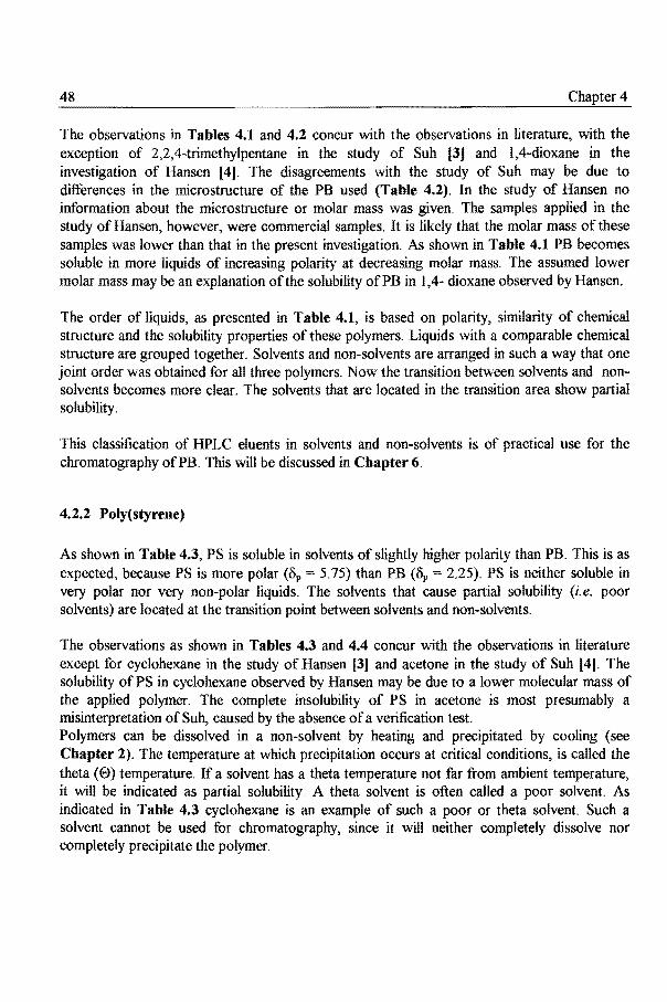
48 4
The observations in Tables 4.1 and 4.2 concur with the observations in literature, with the exception of 2,2,4-trirnethylpentane in the study of Suh [3] and 1,4-dioxane in the investigation of Hansen (4}. The disagreements with the study of Suh may be due to differences in the microstructure of the PB used (Table 4.2). In the study of Hansen no information about the microstructure or molar mass was given. The samples applied in the study ofHansen, however, were commercial samples. It is likely that the molar mass of these samples was lower than that in the present investigation. As shown in Table 4.1 PB becomes soluble in more liquids of increasing polarity at decreasing molar mass. The assumed lower molar mass may be an explanation of the solubility ofPB in 1,4- dioxane observed by Hansen.
The order of liquids, as presented in Table 4.1, is based on polarity, similarity of chemical structure and the solubility properties of these polymers. Liquids with a comparable chemical structure are grouped together. Solvents and non-solvents are arranged in such a way that one joint order was obtained for all three polymers. Now the transition between solvents and nonsolvents becomes more clear. The solvents that are located in the transition area show partial solubility.
This classification of HPLC eluents in solvents and non-solvents is of practical use for the chromatography ofPB. This will be discussed in Chapter 6.
4.2.2 Poly(styrene)
As shown in Table 4.3, PS is soluble in solvents of slightly higher polarity than PB. This is as expected, because PSis more polar (op = 5.75) than PB (ov = 2.25). PS is neither soluble in very polar nor very non-polar liquids. The solvents that cause partial solubility (i.e. poor solvents) are located at the transition point between solvents and non-solvents.
The observations as shown in Tables 4.3 and 4.4 concur with the observations in literature except for cyclohexane in the study of Hansen [3] and acetone in the study of Suh (4]. The solubility of PS in cyclohexane observed by Hansen may be due to a lower molecular mass of the applied polymer. The complete insolubility of PS in acetone is most presumably a misinterpretation of Suh, caused by the absence of a verification test. Polymers can be dissolved in a non-solvent by heating and precipitated by cooling (see Chapter 2). The temperature at which precipitation occurs at critical conditions, is called the theta (0) temperature. If a solvent has a theta temperature not far from ambient temperature, it will be indicated as partial solubility. A theta solvent is often called a poor solvent. As indicated in Table 4.3 cyclohexane is an example of such a poor or theta solvent. Such a solvent cannot be used for chromatography, since it will neither completely dissolve nor completely precipitate the polymer.

Solvent and Non-Solvent Selection
Table 4.3 Solvent and Non-Solvent Selection for Poly(styrene)
1 2 3 4
5 6 7
Solvent name
2,2, 4-Trimethylpentane Diethylether Cyclohexane3) Tetrachloromethane Toluene Dichloromethane Chloroform
Solvent1)
+/- 4)
+ 1-+ + + +
8 9
Tetrahydrofuran + 1,4-Dioxane +
10 N,N-Dimethylacetamide + 11 N,N-Dimethylformamide + 12 Benzyl alcohol + 13 Methyl ethyl ketone + 14 Ethyl acetate + 15 Acetone +/-16 Dimethylsulfoxide 17 Acetonitrile 18 2-Propanol 19 Methanol 20 Water
Non-solvenel
+ +I-+I-
+I-+ + + + +
1) 2)
Solvent and non-solvent test see Chapter 3 Solvent and non-solvent test see Chapter 3 Theta (9) solvent at 35 oc
Not Soluble at Molar Mass (g!mol) RangeS)
>103
>5x10⁴
>5xl05
>5x10⁴
>103
>5x10³
>103
>5x10²
>102
3) 4)+/- = Partially soluble, transitional state from soluble to non-soluble at ambient
temperature and a concentration of 1 mg/ml see Chapter 3 5) Maximum value investigated 106 g/mol (cone. 1 mg/ml)
49
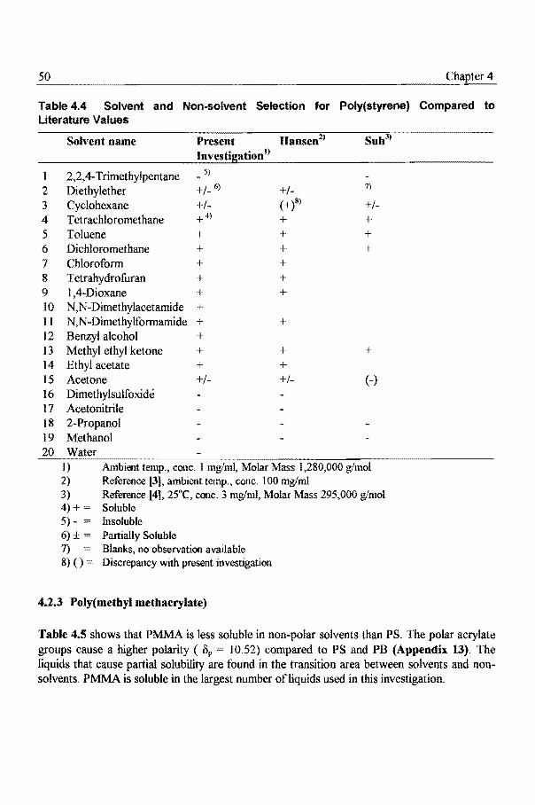
50 4
Table 4.4 Solvent and Non-solvent Selection for Poly(styrene) Compared to Literature Values
Solvent name Present
I 2,2, 4-Trimethylpentane 5)
2 Diethylether +/- 6) +I- 7)
3 Cyclohexane +I- (+)8) +I-4 Tetrachloromethane +4) + + 5 Toluene + + + 6 Dichloromethane + + + 7 Chloroform + + 8 Tetrahydrofuran + + 9 1, 4-Dioxane + + 10 N,N-Dimethylacetamide + II N,N-Dimethylformamide + + 12 Benzyl alcohol + 13 Methyl ethyl ketone + + + 14 Ethyl acetate + + 15 Acetone +I- +I- (-) 16 Dimethylsulfoxide 17 Acetonitrile 18 2-Propanol 19 Methanol 20 Water
l) Ambient temp., cone. I mg/ml, Molar Mass 1,280,000 2) Reference [3), ambient temp., cone. 100 mg/ml 3) Reference [4], 25°C, cone. 3 mg/ml, Molar Mass 295,000 g/mol 4)+ Soluble 5)- Insoluble 6)± Partially Soluble 7) Blanks, no observation available 8)() Discrepancy with present investigation
4.2.3 Poly(metbyl methacrylate)
Table 4.5 shows that PMMA is less soluble in non-polar solvents than PS. The polar acrylate groups cause a higher polarity ( 0p 10.52) compared toPS and PB (Appendix 13). The liquids that cause partial solubility are found in the transition area between solvents and nonsolvents. PMMA is soluble in the largest number ofliquids used in this investigation.

Solvent and Non-Solvent Selection 51
Table4.5 Solvent and Non-Solvent Selection for Poly( methyl methacrylate)
Solvent name Solvent1l Non-solvene> Not Soluble at Molar Mass {g{mol} Range6)
1 2,2, 4-Trimethylpentane + >102
2 Diethylether + >5xl03
3 Cyclohexane + >102
4 T etrachloromethane3 l +/- 5) +I- >5x10⁵
5 Toluene + 6 Dichloromethane + 7 Chloroform + 8 Tetrahydrofuran + 9 1,4-Dioxane + 10 N,N-Dimethylacetarnide + 11 N,N-Dimethylformarnide + 12 Benzyl alcohol + 13 Methyl ethyl ketone + 14 Ethyl acetate + 15 Acetone + 16 Dimethylsulfoxide + 17 Acetonitrile4l +I- +/- >5xl05
18 2-Propanol + >104
19 Methanol + >5x10³
20 Water + >102
1) Solvent and non-solvent test see Chapter 3 2) Solvent and non-solvent test see Chapter 3 3) Theta (B) temperature at 27°C 4) Theta (B) temperature at 30°C 5)+/- Partially soluble, transitional state from soluble to non-soluble at ambient
temperature and a concentration of 1 mg/ml see Chapter 3 6) Maximum value investigated 106 g/mol (cone. 1 mg/ml)
The observations shown in Tables 4.5 and 4.6 concur with the observations in literature with the exception of tetrachloromethane in the study of Hansen [3] and Suh [4]. Another discrepancy is the solubility of PMMA in toluene and acetonitrile observed by Hansen. The solubility of PMMA in tetrachloromethane is a matter of time. It takes more than one day to get PMMA partially dissolved .• The improved solubility of toluene and acetonitrile in the present study is probably caused by the lower concentration applied, compared to the study of Hansen.

52 4
Table4.6 Solvent and Non-solvent Selection for Poly(methyl methacrylate) Compared to Literature Values
Solvent name Present Hansen2) Suh3)
1 2,2,4-Trimethylpentane 2 Diethylether 7)
3 Cyclohexane 5)
4 Tetrachloromethane +/- 6) (-)8) (-) 5 Toluene + 4) (+/-) + 6 Dichloromethane + + + 7 Chloroform + + 8 T etrahydrofuran + + 9 1,4-Dioxane + + 10 N,N-Dimethylacetamide + 11 N,N-Dimethylformamide + + 12 Benzyl alcohol + 13 Methyl ethyl ketone + + + 14 Ethyl acetate + + 15 Acetone + + + 16 Dimethylsulfoxide + + 17 Acetonitrile +/- (-) 18 2-Propanol 19 Methanol 20 Water
I) Ambient temp., cone. 1 mg/ml, Molar Mass 1,300,000 g/mol 2) Reference [3), ambient temp., cone. 100 mg/ml 3) Reference [4), 25°C, cone. 3 mg/ml 4)+ Soluble 5)- Insoluble 6)± = Partially Soluble 7) Blanks, no observation available 8) () = Discrepancy with present investigation

Solvent and Non-Solvent Selection 53
4.3 Conclusions
In the present investigation 80% of the observations concur with the observations in previous publications. The disagreements are located in the transition area between solvents and nonsolvents. Here the polymer solubility strongly depends on the experimental conditions like temperature, polymer concentration, microstructure and molar mass, which might explain the discrepancies. Especially in the transition area the control tests carried out in this investigation are of great help in determining partial solubility.
As expected from the polar solubility parameter of polymer and solvent, it was confirmed that a non-polar polymer is soluble in· more non-polar liquids and a polar polymer is soluble in more polar liquids. The differences in solubility are the basis for a chromatographic separation of polymers based on solubility. The next step will be, to find the solvent/non-solvent composition at which the polymer will precipitate, based on the knowledge of solvents and non-solvents. This will be discussed in Chapter 5.
In this investigation is achieved a classification of solvents and non-solvents for the three polymer standards under the most important chromatographic conditions. Another step forward is the verification test on polymer solubility, insolubility and partial solubility.
As shown in Tables 4.1, 4.3 and 4.5 there are many ways to separate polymers based on solubility differences in pure liquids. Separations can also be obtained by heating and cooling of polymer solutions (as applied in the Baker-Williams fractionation [7]). In the present investigation a choice was made for a separation based on solubility differences between solvent/non-solvent mixtures at constant temperature. This approach is the most practical one for realisation in an HPLC instrument.
An issue of future research may be the investigation of the influence of other HPLC conditions such as pressure and flow. A dissolution study could be performed under dynamic conditions, e.g. with a recycling flow. The molar mass dependency of the solubility and the partial solubility could than be studied in a quantitative manner. Gel Permeation Chromatography (GPC/SEC) will be essential in monitoring this process.

54 4
4.4 References
[1] Glockner, G., Polymer characterisation by liquid chromatography, J. Chromatogr., library vol. 34, Elsevier, Amsterdam (1987)
[2] Brandrup, l, Immergut, E.H., Polymer Handbook, 3rd ed., John Wiley & Sons, New York (1989)
[3] Hansen, C.M.J., Paint Technologies, 39, 104 (1967) [4] Suh, K.W., Corbett, J.M., J. Appl. Polym. Sci, 12, 2359 (1967) [5] Glockner, G., Gradient HPLC of Copolymers and Chromatographic Cross Fractionating,
Springer, Berlin (1991) [6] Mourey, T.H, J. Chromatogr., 357, 101 (1986) [7] Baker, C.A, Williams, R.P.J., J. Chern. Soc. (London) 2356 (1956)

Solubility of Polymers in Solvent/Non-Solvent Mixtures
5. SOLUBILITY OF POLYMERS IN SOLVENT/NON-SOLVENT MIXTURES
55
Summary: The separation of polymers in gradient polymer elution chromatography is strongly related to the cloud-points of polymers. These cloud-points have been determined by the titration of polymer solutions with a non-solvent, which precipitates the polymer. The precipitation point or cloud-point was observed visually. The applied polymers were PB, PS, and PMMA. The selection of proper solvents and non-solvents was described in Chapter 4. An overview of all determined cloud-points is presented for each polymer representing a total of 215 observations. Based on these results information is obtained on solvent and non-solvent strength. This information is of crucial importance for the prediction of the HPLC separation of polymers in a mixture or blend.
5.1 Introduction
5.1.1 Field oflnvestigation
The aim of this chapter is to determine the points of insolubility or cloud-points of the selected polymers in binary solvent/non-solvent mixtures. The solvents and non-solvents are common HPLC eluents ( see Chapter 4). The cloud-point is obtained by adding a non-solvent (precipitant) to a polymer solution [lJ. The cloud-point is defined by a solvent/non-solvent composition. The complete process of non-solvent addition is called turbidity titration.
The cloud-point is correlated with the solvent/non-solvent composition at which the polymer elutes from the HPLC column [2] and it can be used to predict the chromatographic separation of polymers. The aim of this investigation is to study this correlation.
5.1.2 Previous Work
Glockner eta!. [2,3,4,5,6], Quarry eta/. [7], Schultz eta/. [8] and Staal et a/.[9] reported on the correlation between cloud-points and chromatography. Only for a few polymers and copolymers the chromatographically obtained results were correlated with cloud-point observations. Most HPLC publications on polymers could not be used to compare the observed cloud-points to the literature values, because only in a very few cases the original cloud-point observations were presented. In order to compare previous work with the observations in the present investigation, the polymer literature has to be consulted.

56 Chapter 5
Turbidity titration and cloud-point determination became very popular in polymer literature in the sixties. Elias et al. [10,11,14,15,22] and Giesekus [12] improved this analytical method with respect to methodology and instrumentation. Turbidimetric titrations were often applied to obtain the molar mass of polymers or to fractionate polymers.
An overview of cloud-points of poJymers is compiled in the 'Polymer Handbook' by Elias et al. [13]. Most publications mentioned in this handbook, however, cover only a few cloudpoints of interest for this investigation. Only the authors Elias et al. [14,15], Oth et al. [16], Spychaj et al. [17], Turar et al. [18], Chinai et al. [19] and Suh et al. [21] worked with the same polymers and the same solvent/non-solvent combinations as used in the present study.
5.1.3 Missing Infonnation
There has been no systematic study to the determination of cloud-point compositions for the selected polymers and HPLC eluents, under the experimental conditions ofHPLC.
Based on the classification of solvents and non-solvents presented in Chapter 4, many cloudpoint compositions are possible. From all these possible combinations only a very limited number of cloud-point values have been published. Even these values are of limited use because of differences in experimental conditions, molar mass and microstructure of the polymers. Therefore, all the cloud-point values needed for this investigation were determined experimentally.
5.1.4 Present Research
5.1.4.1 Method
Cloud-point determination is based on the isothermal addition of a non-solvent {precipitant) to a homogeneous polymer solution. The first resulting detectable turbidity is called the incipient or initial turbidity [1]. That point represents a solvent/non-solvent composition called the cloud-point composition. The non-solvents needed for this titration were selected in Chapter 4. Cloud-points can be determined visually or by means of a UVIVIS spectrophotometer which measures the intensity of the scattered light of the suspended polymer particles. In the present research the titrimetrically obtained cloud-points have been determined by visual observation.

in Solvent/Non-Solvent Mixtures 57
5.1.4.2 Experimental Conditions
The cloud-point composition depends on experimental conditions (for more details see Chapter 3). The temperature, polymer concentration and molar mass affect the cloud-point composition. At very high molar mass, however, the cloud-point is hardly affected by small variations in experimental conditions (see Appendices 14-16). Therefore, the cloud-point determination is performed with high molar mass (106 g/mol) narrow dispersity polymer standards. This allows for a comparison of cloud-points between different polymer solvent/non-solvent systems.

5.2 Results and Discussion
5.2.1 Experimental Cloud-Point Values of Poly(butadiene)
5.2.1.1 Previous Work
It was not possible to compare the experimental cloud-point observations (Table 5.1) with observations obtained from literature due to the fact, that other solvents and non-solvents were used and also because the PB samples were different with respect to their microstructure.
5.2.1.2 Single Solvent Solubility Versus Solvent/Non-Solvent Solubility
The cloud-point results shown in Table 5.1 are derived from the solubility and insolubility results presented in Chapter 4 (Table 4.2 ). All liquids as determined to be non-solvents in Table 4.2 resulted in a cloud-point during the titration of the different PB solutions, with the exception of 1,4-dioxane. Only one combination with 1,4-dioxane gave a cloud-point. This phenomenon is not completely unexpected, because 1,4-dioxane is located in the transition region between solvents and non-solvents. In this region weak non-solvents can be expected.
A clear example of such a weak non-solvent is 2,2,4-trimethylpentane. As shown in Table 4.2, PB is partially soluble in 2,2,4-trimethylpentane (weak non-solvent). During titration of a PB solution with 2,2,4-trimethylpentane no cloud-point , occurs. Once the polymer has been dissolved, nearly all solvent molecules that are interacted with the polymer can be exchanged by non-solvent molecules without affecting polymer solubility. This process is called cosolvency (20}. Such a non-solvent will be called an apparent non-solvent (A) in this investigation (for more details see Chapter 3).

Solubility ofPolymers in Solvent/Non-Solvent Mixtures 59
Table 5.1 Experimental Cloud-Point Values of Poly(butadiene)1l
Non-Solvents Solvents Average7J NS
26) 3 6 4 5 7 8 Strength %NS/S in%S
2,2,4-Trimethyl A9) A A A A A A pentarre
2 Diethyl ether ~)
3 Cyclohexane 4 Tetrachloro
meiliane 5 Toluene 6 Dichloro
methane 7 Chloroform 8 Tetrahydrofuran 9 1,4-Dioxane A A A A A A 83/17 (17) 14 Ethyl acetate 51/49 79/21 66/34 77/23 77/23 74/26 80/20 28 13 Methyl ethyl 48/52 75/25 67/33 74/26 72/28 68/32 73/27 32
ketone 12 Benzyl alcohol 41/59 37/63 63/37 44/56 44/56 55/45 47/53 53 15 Acetone 23/77 47/53 41/59 49/51 48/52 46/54 47/53 57 10 N,N-Dimethyl 37/63 21/79 38/62 40/60 40/60 42/58 47/53 62
acetamide 18 2-Propanol 10/90 31/69 40/60 37/63 35/65 44/56 45/55 65 11 N,N-Dimethyl 24/76 --2) 29/71 31/69 32/68 35/65 38/62 68
fermamide 17 Acetonitrile 9/91 22/78 24/76 27/73 28/72 25/75 78 16 Dimethyl 12/88 18/82 19/81 22/78 26/74 25/75 80
sulfoxide 19 Methanol 5/95 19/81 17/83 19/81 23/77 25/75 82 20 Water 6/94 (94) Average Solvent S)
Strength in %NS 26 363) 40 41 42 44 454)
1) = Molar mass 967,000 g/mol, ambient temperature and a concentratien of 1 mg/ml solvent 2) -- = Immiscible liquids 3) = Expected value 4) = Water and 1,4-Dioxane excluded 5) Open places = mixtures of solvents 6) Corresponds to the numbering of liquids in the first column. 7) Average% of solvent ofthe cloud-points for all solvents in combination with the same non-solvent. 8) Average% of non-solvents ofthe cloud-points for all non-solvents in combination with the same
solvent. 9) A= Apparent non-solvent (no cloucl-point observed duting titration)

60 5
The numbering of the liquids in the first column of Table 5.1 is the same nurnbering as in Table 4.2. It is based on a joint order of solvents and non-solvents for PB, PS and PMMA. The nurnbering of the liquids in the heading of Table 5.1 also corresponds to the nurnbering in Table 4.2.
These liquids in the heading of Table 5.1 are solvents for PB (see Table 4.2). In the first column all applied liquids are present. The open places corresponds to mixtures of solvents for PB. All other positions are non-solvents or poor non-solvents (A- solvents).
The cloud-point composition consists of the % non-solvent (left number) and the % solvent (right number). In a few cases solvent/non-solvent cornbinations could not be tested due to immiscibility of solvent and non-solvent. More details of solvent/non-solvent miscibility are presented in Appendices 5 and 6.
Ethyl aretate
.I ---·-·>
Solvents
Figure 5.1: Schematic three-dimensional representation co vering the c/oud-point values trom Table 5.1 tor poly(butadiene) ( region of insolubility).

Solubility of Polymers in Solvent/Non-Solvent Mixtures 61
In order to discover any possible coherence between the cloud-points in Table 5.1, the average % non-solvent is calculated for each column (bottom row). This % represents the average solvent strength for each solvent. For each row the average % solvent is calculated, representing the average strength of each non-solvent. The solvent and non-solvent strength is discussed in more detail when the results of Table 5.2 and Figure 5.2 are discussed. All rows are ranked in the order of increasing non-solvent strength. All columns are ranked in the order of increasing solvent strength.
Table 5.2 Solvent Strength Determination for Poly(butadiene)11
Solvent
Tetrahydrofuran Chloroform Dichloromethane Tetrachloromethane Toluene Cyclohexane Diethyl ether
1) Molar mass 967,000 g/mol
Non-Solvent % 2-Propanoe>
45 44 40 37 35 31 10
Average31
% Non-Solvent
45 44 40 41 42 36 26
2) Row 18 from Table 5.1, cloud-point va lues at ambient temperature and at a concentration of 0.1 % w/v
3) Bottom row Table 5.1
The general trends between the cloud-point values are visualised in Figure 5.1. In this tigure the % non-solvent is added as third axis to the two-dimensional presentation in Table 5.1. The result is a three-dimensional figure, representing all cloud-points or the region of insolubility for PB. The polymer/solvent/non-solvent system PB-diethyl ether - methanol gives a minimum cloud-point value and the system PB-tetrahydrofuran - ethyl acetate gives a maximum cloudpoint value. The explanation is that the cloud-point is influenced by the polarity of the polymer, the polarity of the solvent and the pclarity of the non-solvent. For example the minimum cloud-point value is caused by the combination of the most non-polar solvent for PB, diethyl ether, and the very polar non-solvent methanol. The maximum cloud-point value is caused by the combination of the most polar solvent for PB tetrahydrofuran and the less po lar non-solvent ethyl acetate.

62 Chapter 5
(A) 0% 50% 100% Tetrahydrofuran Cl oud-Point Medium
Strong Insolu~le . . Solvent F_hZTlLZ2 '-L~---~-~-~--~g
Soluble 2-Propanol 100% 50% 0%
fZ172Z/Z~~~4 Poor Medium Strong
(B) 0% 50% 100% Diethyl ether
Cloud-Point Poor
r/7?ZAZMZiZf727////~tnt 2-Propanol 100% 50% 0%
Figure 5.2: lnfluence of a strong solvent (A) (tetrahydrofuran) and a poor solvent (8) (diethyl ether) on the 2-propanol scale tor poly(butadiene).
The consequence of the increase of cloud-point values on the solubility of PB can be illustrated by two examples. First, all solutions of PB (dissolved in different solvents) are titrated with the non-solvent 2-propanol. Second, the solution of PB dissolved in tetrahydrofuran is titrated with different non-solvents. The advantage of 2-propanol and tetrahydrofuran is that these liquids are miscible with all the other liquids.
The first example is the horizontal row of cloud-point values in Table 5.1, representing all solutions of all PB solvents applied, titrated with the non-solvent 2-propanol. These cloudpoints are ranked according to the amount of 2-propanol required to reach the cloud-point as given in Table 5.2. Diethyl ether requires the lowest and tetrahydrofuran the highest amount of 2-propanol to reach the cloud-point composition. The importance of this ranking is that it represents the solvent strength. The effect of the solvent strength is illustrated in Figure 5.2.

Solubility of Polymers in Solvent/Non-Solvent Mixtures 63
The cloud-point composition is the result of a competition between solvent and non-solvent to dissolve or to precipitate the polymer. The solvent has an attractive and the non-solvent a repelient interaction with the polymer. At 50% solvent/non-solvent both interactions are in balance.
As shown in Figure 5.2, the solvents can be divided into poor, moderately strong and strong solvents. A strong solvent only requires a low % solvent to dissolve the polymer. A poor solvent needs a high % solvent to dissolve the polymer. For a proper comparison of the solvent strength, the samenon-solvent (2-propanol) is applied here. In Table 5.2. the solvent strength is now expressed in% 2-propanol. In the case of astrong solvent (Figure 5.2) a high % 2-propanol is needed to compensate for the strength of the solvent. In the case of a poor solvent only a low % 2-propanol is needed to compensate for the strength of the solvent. Table 5.2 shows that tetrahydrofuran is the strongest of the selected solvents and di ethyl ether is the poorest solvent. The average solvent strength has a comparable trend related to the 2-propanol value with the exception of the order of dichloromethane, tetrachloromethane and toluene. The advantage ofthe 2-propanol solvent strength scale is that only a few experiments are needed to define it. The disadvantage is related to the question to what degree this scale is representative for all other non-solvents (specific interactions). The advantage ofthe average solvent strength scale is that it represents many different non-solvents. The disadvantage is that many experiments are needed and some important experiments are not possible due to the immiscibility of the liquids.
Table 5.3 Non-Solvent Strength Determination for Poly(butadienef1
Non-Solvent Solvene> Average3>
Water Methanol Dimethyl sulfoxide Acetonitrile N,N-Dimethylformamide 2-Propanol N,N-Dimethylacetamide Acetone Benzyl alcohol Methyl ketone Ethyl acetate 1,4-Dioxane
% Tetrahydrofuran % Solvent 94 (94) 75 82 75 80 75 78 62 68 55 65 53 62 53 57 53 53 27 32 20 28 17 (17)
1) Molar mass poly(butadiene) 967,000 glmol 2) Column 8 Table 5.1, cloud-point values at ambient temperature and at a concentration of0.1 % w/v 3) Last column Table 5.1
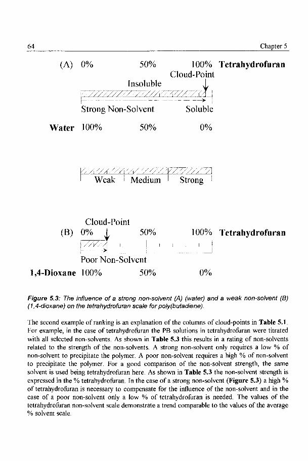
64 Chapter 5
(A) 0% 50% 100% Tetrahydrofuran Cl oud-Point
F7~/00?di Strong Non-Solvent Soluble
Water 100% 50% 0%
Cloud-Point (B) P/t, '
5
~%'-~-=~o/ï Tetrahydrofuran
Poor Non-Solvent
1 ,4-Dioxane 100% 50% 0%
Figure 5.3: The influence of a strong non-solvent (A) (water) and a weak non-solvent (8) (1,4-dioxane) on the tetrahydrofuran scale tor poly(butadiene).
The second example of ranking is an explanation of the columns of cloud-points in Table 5.1. For example, in the case of tetrahydrofuran the PB solutions in tetrahydrofuran were titrated with all selected non-solvents. As shown in Table 5.3 this results in a rating of non-solvents related to the strength of the non-solvents. A strong non-solvent only requires a low % of non-solvent to precipitate the polymer. A poor non-solvent requires a high % of non-solvent to precipitate the polymer. For a good comparison of the non-solvent strength, the same solvent is used being tetrahydrofuran here. As shown in Table 5.3 the non-solvent strength is expressed in the % tetrahydrofuran. In the case of a strong non-solvent (Figure 5.3) a high % of tetrahydrofuran is necessary to compensate for the influence of the non-solvent and in the case of a poor non-solvent only a low % of tetrahydrofuran is needed. The values of the tetrahydrofuran non-solvent scale demonstrate a trend comparable to the values of the average % solvent scale.

Solubility ofPolymers in Solvent/Non-Solvent Mixtures 65
5.2.1.3 Practical Application
The presentation of the solvent and non-solvent strength in Figures 5.2 and 5.3 is of practical use to the chromatography ofpolymers. This presentation metbod invalving the position ofthe polymer has an analogy with a chromatogram, since in the chromatography of polymers the gradient starts with the non-solvent and ends with the pure ( or a high %) solvent.
The practical importance ofthe solventand non-solvent scales in Tables 5.2 and 5.3 is that in applying different solvent/non-solvent combinations the polymer can be located in many different positions within the gradient chromatagram and this is the basis for an efficient separation of mixtures of polymers.
5.2.2 Experimental Cloud-Point Values of Poly(styrene)
5.2.2.1 Previous Work
The cloud-point values from Iiterature (Appendix 11) agree well with the experimental values presented in Ta bie 5.4. This particularly holds when the differences in experimental conditions (concentration and molar mass) are taken in account Two exceptions are the solvent/nonsolvent systems tetrahydrofuran-methanol and tetrachloromethane-acetone. These values have been duplicated many times with an experimental error of+/- 0.5% (% non-solvent) (see Appendix 11). For the tetrahydrofuran-methanol system reference [25} gives the same clouclpoint as observed in the present investigation. It therefore becomes more likely that the observation in reference [14} is wrong. It is known that impurities and stabilisers in the solvents can cause this deviations (22}.
Poly(styrene) is the most extensively examined polymer. In spite of that, only a smal! part ( 18%) of the present observations could be compared with Iiterature values.
5.2.2.2 Single Solvent Solubility Versus Solvent/Non-Solvent Solubility
All the non-solvents determined in Chapter 4 (Table 4.4) caused a cloud-point as shown in Table 5.4. The solvents causing partial solubility in Table 4.4 proved not all the expected partial solubility in cloud-point experiments, Iike cyclohexane. Diethyl ether and acetone (partial solubility), however, proved to be (very weak) non-solvents and worked as an apparent non-solvent in some combinations.

Table 5.4 Experimental Cloud-Point Values of Poly(styrene)11
Non-Solvents 36)
%NS/%S 4 5
Solvents 6 7 8 9 10 11 12 13 14
Average7) NS-strength
in %-Solvenfll
1 2,2,4-Trimethylpentane 12/88 43/572) 49/51 67/33 65/35 55/45 50!50 39/61 37/63 49
2 Diethyl ether A9) 86/14 90/10 86/14 87/13 89/11 81/19 A 80/20 A 83/17 80/20 15
3 Cyclohexane A A A A A A A A A A A A 4 Tetrachloromethane 5 Toluene 6 Dichloromethane 7 Chloroform 8 Tetrahydrofuran 9 1,4-Dioxane 10 N,N-Dimethylacetamide 11 N,N-Dimethylformamide 12 Benzyl alcohol 13 Methyl ethyl ketone 14 Ethyl acetate 15 Acetone A 83117 85/15 71129 76/24 85/15 82/18 79/21 75/25 85/15 56/44 46/54 25 16 Dimethyl sulfoxide 50/50 52/48 55/45 69/31 63/37 41/59 55145 46/54 44/56 57/43 44/56 48 17 Acetonitrile 44/56 53/47 46/54 52/48 53/47 36/64 32/68 22/78 47/53 19/81 13/87 62 18 2-Propanol 16/844
) 32/68 33/67 43/57 43/57 49/51 44/56 47/53 42/58 25175 18/82 17/83 64 19 Methanol 21/79 23/77 26/74 27/73 40/60 28/72 35/65 20/80 17/83 12/88 8/92 77 20 Water - 2
) 10/90 6/94 4/96 2/98 94 Averal!e solvent !:trtmoth8
) in %NS4) 51 55 56 60 62 52 50 48 44 41 35
1) Molar mass 1,280,000 glmol, ambient temperature and a concentration of 1 mglml 2) --"'Immiscible liquids. 3) water excluded 4) Molar Mass 66,000 glmol 5) Cyclohexane excluded 6) Corresponds to the numbering of liquids in the first column 7) Average % of solvent of the cloud-points for all solvents in combination with the same non -solvent 8) Average% of non-solvent of the cloud-points for all non-solvents in combination with the same solvent 9) A= Apparent non-solvent (no cloud-point observed during titration)

Solubility ofPolymers in Solvent/Non-Solvent Mixtures 67
The ranking of solvents and non-solvents in Table 5.4 was the same as in Table 4.4. This ranking was based on a joint order of solvents and non-solvents for all three polymers as discussed in Chapter 4. The result of this ranking is a closed region of insolubility. Another result of this ranking in the case ofPS is, that the strongest solvents are located in the middle, and the poorest solvents at the beginning and end of the average solvent strength row (Table 5.4). Also, the strongest non-solvents are the first (most non-polar) and the last (most polar) liquids in the average non-solvent strength column (Table 5.4).
\
~··----)>
Solvents
Figure 5.4: Schematic three-dimensional presentation covering the cloud-point values of Table 5.4 for poly( styrene) (regions of insolubility).
As compared to PB (Figure 5.1), PS has two regions of insolubility. These regions are shown in the three-dimensional plot of Figure 5.4, which is based on the observations in Table 5.4. These two regions are caused by the polarity of the non-solvent and the polarity of the polymer. PSis a more polar polymer than PB and will not dissolve in 2,2,4-trimethylpentane and only partially in diethylether. In comparison with PB, PS is soluble in liquids with a higher polarity such as ethyl acetate.
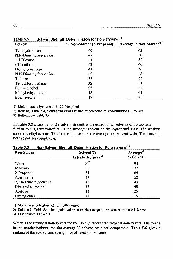
68 5
Table 5.5 Solvent Strength Determination for Poly(styrene)11
Solvent %Non-Solvent (2-Propanol)2> Average %Non-Solvent3)
Tetrahydrofuran 49 62 N,N-Dimethylacetamide 47 50 1,4-Dioxane 44 52 Chloroform 43 60 Dichloromethane 43 56 N,N-Dimethylformamide 42 48 Toluene 33 55 Tetrachloromethane 32 51 Benzyl alcohol 25 44 Methyl ethyl ketone 18 41
1) Molar mass poly(styrene) 1,280,000 g/mo1 2) Row 18, Table 5.4, cloud-point values at ambient temperature, concentration 0.1 % w/v 3) Bottom row Table 5.4
In Table 5.5 a ranking of the solvent strength is presented for all solvents of polystyrene. Similar to PB, tetrahydrofuran is the strongest solvent on the 2-propanol scale. The weakest solvent is ethyl acetate. This is also the case for the average non-solvent scale. The trends in both scales are comparable.
Table 5.6 Non-Solvent Strength Determination for Poly(styrene)11
Non-Solvent Solvent% Average3>
Tetrahydrofuran2> % Solvent
Water Methanol 2-Propanol Acetonitrile 2,2,4-Trimethylpentane Dimethyl sulfoxide Acetone Diethyl ether
1) Molar mass poly(styrene) 1,280,000 g/mol
902) 94
60 77 51 M 47 62 45 37 15 11
49 48 25 15
2) Colunm8, Table 5.4, cloud-point values at ambient temperature, concentration OJ% w/v 3) Last column Table 5.4
Water is the strongest non-solvent for PS. Diethyl ether is the weakest non-solvent The trends in the tetrahydrofuran and the average % solvent scale are comparable. Table 5.6 gives a ranking of the non-solvent strength for all used non-solvents.

Solubility of Polymers in Solvent/Non-Solvent Mixtures 69
5.2.3 Experimental Cloud·Point Values ofPoly(methyl methacrylate)
5.2.3.1 Previous Work
The cloud-point values obtained from literature (see Appendix 12), agree with the experimental values (Table 5. 7), except for the solvent/non-solvent combinations tetrachloromethane - methanol and acetone - methanol. As the experimental conditions do not cause these differences, there are two possible explanations: the rate of precipitation and the quality of the solvents. The first possibility is that methanol in combination with PMMA gives a time-dependent precipitation mechanism, i.e. it takes some time before PMMA precipitates. This phenomenon was already observed by Gieskus [12] and was also observed sometimes for PMMA in this investigation. In that case a surplus non-solvent can be added before visible precipitation occurs. The values for methanol were reproducible and were at the right level compared to the other methanol-solvent combinations. The second possibility can be found in Elias [22]: impurities and stabilisers in the solvents can cause serious deviations in the cloudpoint composition.
The order of solvents and non-solvents in Table 5. 7, is different from the order for PS (Table 5.4). The more polar solvents in particular dimethyl sulfoxide and N,N-dimethylformamide are strong solvents. As in the case ofpoly(styrene), the strongest solvents for PMMA are located in the middle position of the bottom row in Table 5. 7. This is visualised also in the schematic three-dimensional presentation of the space ofinsolubility (Figure 5.5).
5.2.3.2 Single Solvent Solubility Versus Solvent/Non-Solvent Solubility
All non-solvents listed in Chapter 4, Table 4.6, caused a cloud-point as shown in Table 5.4. The liquids causing partial solubility turned out to be apparent non-solvents.

Table 5.7 Experimental Cloud-Point Values of Poly(methyl methacrylate)11
Non-Solvents 5 6 7 11 16
Solvents 12 17 10 9 13 15 8
Average5> 14 NS-Strength
in %-Solvent_
1 2,2,4-Trimethylpentane 3 Cyc1ohexane 2 Diethyl ether 4 Tetrachloromethane 5 Toluene 6 Dichloromethane 7 Chloroform 8 Tetrahydrofuran 9 1.4-Dioxane 10 N,N-Dimethylacetamide 11 N,N-Dimethylformamide 12 Benzyl alcohol 13 Methyl ethyl ketone 14 Ethyl acetate 15 Acetone 16 Dimethyl sulfoxide 17 Acetonitrile 18 2-Propanol 19 Methanol 20 Water
7/93 21179 57/43 63/37 37/63 32/68 34/66 30/70 27173 7/93 30170 68/32 77/23 54/46 46/54 49/51 47/53 52/48 40/60 43/57
30170 50150 80/20 75/25 80/20 68/32 80/20 67/33 80/20 75/25 69/31 68/32 62/38 63/37 ~ A A A A A A A A A A A A A
A A A A A A A A A A A A A A 60/40 64/36 82118 90/10 76/24 82/18 80/20 78/22 75/25 73/27 62/38 67/33 60/40 58/42 65/35 66/34 77/23 80/20 75/25 81119 82/18 66/34 76/24 77/23 64/36 61139 67/33 59/41
--2) 9/91 9/91 15/85 15/85 18/82 16/84 24/76
Average solvent strength 34 46 73 77 773) 773
) 74 703) 693) 623
) 55 543) 523> 50
in %NS6l
I) Molar mass 1,300,000 glmol, ambient temperature and a concentration of 1 mglrnl 2) --=immiscible liquids 3) Water excluded 4) Corresponds to the numbering of the liquids in the first column 5) Average %of solvent of the cloud-points for all solvents in combination with the same non-solvent 6) Average% of non-solvent of the cloud-points for all non-solvents in combination with the same solvent 7) A= Apparent non-solvent (no cloud-point observed during titration)
66 53 32
28 29 85

Solubility of Polymers in Solvent/Non-Solvent Mixtures 71
Much like PS, PMMA is a more polar polymer. PMMA for example is soluble in polar solvents such as acetone and dimethyl sulfoxide. The order of the solvent and non-solvent strength is different in relation to PB and PS.
i -Solvents g >. ~ 0 ~
>!1
Figure 5.5: Schematic three-dimensional presentation covering the cloud-point values of Table 5.7 for poly( methyl methacrylate) (regions of insolubility).
PMMA has two regions of insolubility as shown in the three-dimensional presentation in Figure 5.5. Both regions show a maximum cloud-point level representing the strongest solvents.

72 Chapter 5
Table 5.8 Solvent Strength Determination for Poly(methyl methacrylate)11
Solvent Non-Solvent% 2-Propanoe) Average% Non-Solvent3)
Chloroform 902) 77 Dichloromethane 82 73 Dimethyl sulfoxide 82 77 Benzyl alcohol 80 74 Acetonitrile 78 70 N,N-Dimethylformamide 76 77 N,N-Dimethylacetamide 75 69 1,4-Dioxane 73 62 Acetone 67 54 Toluene 64 46 Methyl ethyl ketone 62 55 Tetrahydrofuran 60 52 Tetrachloromethane 60 34
I) Molar mass poly(methyl methacrylate) 1,300,000 g!mol 2) Row 18 from Table 5. 7, cloud-point values at ambient temperature and at a concentration of 0.1 %
w/v 3) Bottom row Table 5.7
According to the 2-propanol scale (Table 5.8), chloroform is the strongest solvent and tetrahydrofuran now belongs to the medium strong solvents. Very polar solvents like dimethyl sulfoxide are now strong solvents. This makes the solvent strength of chloroform remarkable. The explanation may be the high dipole moment of chloroform, that interact with polar acrylate groups (sterically attractive).
The trend in the 2-propanol scale and the average non-solvent scales are comparable, with a few exceptions.
Table 5.9 Non-Solvent Strength Determination for Poly(methyl methacrylate)11
Non-Solvent Solvent% Tetrahydrofuran2) Average% Solvent3)
Water 76 85 2,2, 4-Trimethylpentane 69 66 Cyclohexane 60 53 2-Propanol 40 28 Diethyl ether 38 32 Methanol 33 29
I) Molar mass poly(methyl methacrylate) 1,300,000 g!mol 2) Column 8 Table 5.7, cloud-point values at ambient temperature and at a concentration ofO.l % w/v 3) Last column Table 5. 7

Solubility of Polymers in Solvent/Non-Solvent Mixtures 73 ~-----------------------------
We can see in Table 5.9 that water is still the strongest non-solvent for PMMA, but because of the higher polarity of PMMA in relation to PB and PS, the repulsion of 2,2,4-trimethylpentane is so great, that it has become the second strongest non-solvent. The trends shown by the tetrahydrofuran and the average % solvent scale are comparable.
5.2.3.3 Practical Application
The aim of this investigation is to predict the chromatographic separation of polymers. This separation is based on differences in solubility properties between different polymers.
To illustrate how strongly different the effects (in terms of cloud-points) of solvents and nonsolvents can be on the three polymers, the tetrahydrofuran-methanol system was chosen. The cloud-points are: PB 75% methanol, PS 60% methanol and PMMA 33% methanol. Such large differences provide an excellent basis for polymer fractionation and HPLC separation.

74 Chapter 5
5.3 Conclusions
Turbidimetric titration is a fast and reliable method to obtain the cloud-point composition for high molar mass polymers. Only 28 out of215 cloud-point observations (13%) obtained from previous publications were suitable for comparison with the present investigation. Of the 28 observations selected 24 (86%) agree with previous literature [14-26]. We can assume that the 14% deviations are related to problems with solvent quality in the past [22].
The solvent and non-solvent selection tests of Chapter 3 and used in Chapter 4 proved to be very reliable in predicting which solvent and non-solvent combination results in a cloud-point. The regions of insolubility are a characteristic fingerprint of a polymer. In 95% of all tested combinations, the selected non-solvents had a cloud-point. In 5% of all combinations the nonsolvent appeared to be an apparent non-solvent. All these deviations were located in the transition area between solvents and non-solvents.
The results described in this chapter demonstate that considerable progress is made by providing an overview of the cloud-points for the three standard polymers in HPLC solvents, under the most important HPLC conditions. Additional information was obtained concerning the solvent and non-solvent strength. This solvent and non-solvent strength is different for each type of polymer. The differences are caused by the polarity of the polymer. A more polar polymer like PMMA is attracted to more polar solvents and non-solvents. Based on these general rules only general trends can be obtained, because many disturbing factors are playing a secondary role. A more detailed overview of trends and the prediction of cloud-points based on solubility parameters will be presented in Chapter 7.
The practical importance ofthese cloud-points is that they allow the prediction of the position and the separation of polymers in the chromatogram. If the chromatographic separation is based on a polymer solubility mechanism, which can be achieved by choosing the proper solvent/non-solvent combination, the polymer will elute from the HPLC column when it reaches the cloud-point composition. On the basis of the obtained ranking of solvent and nonsolvent strength, each polymer has many different cloud-point compositions, which form the basis for the separation of polymer mixtures. The applications of these results will be discussed in Chapter 6.
A point of future research may be the testing of cloud-points under the dynamic conditions present in the HPLC instrument, i.e. flow and high pressure. The gradient HPLC instrument itself (without column) can be used to generate the cloud-point and the complete turbidity curve.

Solubility of Polymers in Solvent/Non-Solvent Mixtures
5.4 References
[1] Slatsko, A., Elias, H-G., Angew. Makromol. Chern., 23, 29 (1972) [2] Glockner, G., Chromatographia, 25, 854 (1988) [3] Glockner, G., Barth, H.G., J. Chromatogr., 499, 645 (1990) [4] Glockner, G., Wolf, D., Chromatographia, 34, 363 (1992)
75
[5] Glockner, G., Schmutzler, S., Engelhardt, H., Schultz, R., Chromatographia, 25, 983 (1988)
[6] Glockner, G., Wolf, D., Engelhardt, H., Chromatographia, 32, 107 (1991) [7] Quarry, M.A., Stadalius, M.A., Mourey, T.H., Snyder, LR., J. Chromatogr., 358, 1
(1986) [8] Schultz, R., Engelhardt, H., Chromatographia, 29, 205 (1990) [9] Staal, WJ., Jansen, J.AJ., Cools, P., VanHerk, A.M., German, A.L., Proceedings ofthe
Technical Symposia on GPC and the Analysis of Polymers and Additives, Waters Chromatography, San Francisco, Cal., U.S.A. (Oct. 1991)
[1 0] Elias, H-G., Tung, LH., Fractionating of Synthetic Polymers, Dekker, New York {1977) [11] Elias, H-G., Makromol. Chern., 33, 140 (1959) [12] Giesekus, H., Kolloid-Z., 158, 35 {1958) [13] Brandrup, J. Immergut, E.H., Polymer Handbook, 3rd ed., John Wiley & Sons, New
York (1989) [14] Elias, H-G., Etter, 0., Makromol. Chern., 66, 56 (1963) [15] Elias, H-G., Gruber, U., Makromol. Chern., 78, 72 (1964) [16] Oth, J.V., Desreux, Bull. Soc. Chim. Beige, 63,285 (1954) [17] Spychaj, T.D., Lath, D., Berek, D., Polymer, 20, 437 (1979) [18] Turar, Z., Kratchovil, P., Col!. Czech. Corum., 32, 3358 (1967) [19] Chinai, S.N., Valles, R.J., J. Polymer Sci., 39, 363 {1959) [20] Barton, A.F.M., CRC Handbook of Solubility Parameters, CRC Press Inc., Boca Raton,
Florida {1983) [21] Suh, K.W., Corbett, J.M., J. Appl. Polym. Sci., 12,2359 (1968) [22] Elias, H-G., Etter, 0., MakromoL Chern., 89, 228 (1965) [23] Shalliker, R.A., Kavanagh, P.E., J. Chromatogr., 543, 157 (1991) [24] Shalliker, R.A., Kavanagh, P.E., Russel I.M., J. Chromatogr., 558,440 (1991) [25] Glockner, G., Chromatographia, 25, 854 (1988) [26] Schultz, R., Engelhardt, H., Chromatographia, 29, 205 (1990)

76

The Chromatography of High Molar Mass Polymers 77
6. THE CHROMATOGRAPHY OF HIGH MOLAR MASS POLYMERS
Summary: The aim of this investigation is to predict the chromatographic separation of high molar mass polymers, based on a solubility mechanism. So far results have only been published for polystyrene applying a few nonsolvent/solvent combinations. In this chapter more non-solvent/solvent combinations are applied and the present study also includes the polymers poly(butadiene) and poly(methyl methacrylate). The solubility of these polymers in non-solvent/solvent systems is described in Chapter 5 applying the titrimetrically obtained cloud-points. The chromatographically obtained cloud-points in this chapter correlate well with the titrimetrically obtained cloud-points. Based on these results the elution order of the chromatographic separation can be predicted for the three polymers in a mixture. The correlation can become worse when adsorption effects are operative. The adsorption of high molar mass polymers on stationary phases, however, appears to be an exception.
6.1 Introduction
6.1.1 Field of Investigation
The aim of the work described in this chapter is to obtain a liquid chromatographic separation of polymers, exclusively based on a precipitation - redissolution principle. The benefit of such a mechanism is, that the separation can be predicted from titrimetrically obtained cloud-point values, as listed in Chapter 5. To prove the correctness of this approach, the turbidimetrically determined cloud-point values will be correlated to the chromatographically determined cloudpoint values. A condition for such a correlation is the absence of adsorption of the polymer.
6.1.2 Previous Work
Glockner [l] was the first to describe a mechanism for the HPLC separation of polymers based on a non-solvent/solvent gradient. During this gradient the polymer molecules undergo a series of precipitation and redissolution processes along the HPLC column, until they finally elute at a mobile phase composition which is barely a solvent for the specific polymer. Glockner called this separation process High Performance Precipitation Liquid Chromatography (HPPLC). He obtained a good correlation between turbidimetric and chromatographic cloud-points for high molar mass polymers. Schultz et a/. [2], Shalliker et al. (3] and Quarry eta/. [4] described similar correlations. Schultz [2] and Shalliker [5] further reported solvent/non-solvent compositions at which polymers showed adsorption to the

78 Chapter 6
stationary phase in the HPLC column. In general, the separation of high molar mass polymers is based on a precipitation- redissolution process [1].
Many other mechanisms have been proposed to describe the chromatography of polymers. Quarry [4] modified the mechanism suggested by Glockner [1] in a simple 'on-off model, where initially polymer molecules stick to the column and then elute by the mobile phase with no reattachment. Boehm et al. [6] proposed a mechanism that considered polymer elution at eluent compositions applied in critical chromatography [7]. This chromatographic mode is located at the transition point between adsorption and size exclusion. Quarry et al. [8] and Lochmiiller et a!. [9] stated that an adsorption mechanism is always present and that polymer elution still obeys the principals of a normal chromatographic adsorption and desorption process. For example, Mori [10] did most of his polymer HPLC separations based on such an adsorption process. He called this process Liquid Adsorption Chromatography (LAC). The conclusion that can be drawn, from the available data, is that the mechanism of HPLC separation for high molar mass polymers is still not completely understood and requires additional research.
Because there are many different mechanisms active in the gradient HPLC separation of polymers, Cools et al. [7] and Staal et al. [11] suggested to apply the more general name Gradient Polymer Elution Chromatography (GPEC), which does not imply a specific separation mechanism, but covers the application field of polymers and gradient elution separation technology. All the previous names for the different isocratic and gradient types of chromatography of polymers are collectively called Non-Exclusion Liquid Chromatography techniques (NELC) [1].
To obtain a pure precipitation - redissolution mechanism, adsorption of the redissolved polymer on the stationary phase must . be avoided. When the redissolved polymers are adsorbed (or retained) on the stationary phase, they are eluted in the gradient at a higher volume fraction of the (strong) solvent than predicted from cloud-point data. In general adsorption can be expected when poor solvents are applied [11]. Therefore, the application of poor solvents must be avoided. These poor solvents are identified in the solubility observations presented in Chapter 4.
As described by Shalliker [5] and Schultz [2] polymers can adsorb on silica (Si) and octadecyl modified silica (Cis) stationary phases as well. The disadvantage of applying a strongly polar Si phase is the adsorption of polar polymers, polar solvents and polar non-solvents to such a phase. The disadvantage of applying a non-polar Cis phase is the adsorption of non-polar polymers, non-polar solvents and non-polar non-solvents. In the case of the precipitation -redissolution mechanism a stationary phase with a low adsorption capacity is necessary.
As known from HPLC studies on small molecules, there is a stationary phase that shows a low adsorption capacity for polar and non-polar molecules [12]. This is the cyano-propyl-modified (CN) silica stationary phase. This phase belongs to the heterogeneous phases. The
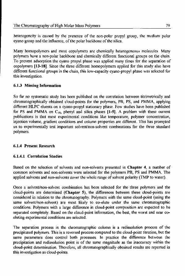
The Chromatography of High Molar Mass Polymers 79
heterogeneity is caused by the presence of the non-polar propyl group, the medium polar cyano group and the influence, of the polar backbone of the silica.
Many homopolymers and most copolymers are chemically heterogeneous molecules. Many polymers have a non-polar backbone and chemically different functional groups on the chain. To prevent adsorption the cyano propyl phase was applied many times for the separation of copolymers [13-18]. Since the three different homopolymers applied for this study also have different functional groups in the chain, this low-capacity cyano-propyl phase was selected for this investigation.
6.1.3 Missing Information
So far no systematic study has been published on the correlation between titrimetrically and chromatographically obtained cloud-points for the polymers, PB, PS, and PMMA, applying different HLPC eluents on a cyano-propyl stationary phase. Few studies have been published for PS and PMMA on C1s, phenyl and silica phases [1-5). A problem with these current publications is that most experimental conditions like temperature, polymer concentration, injection volume, gradient conditions and column properties are different. This has prompted us to experimentally test important solvent/non-solvent combinations for the three standard polymers.
6.1.4 Present Research
6.1.4.1 Correlation Studies
Based on the selection of solvents and non-solvents presented in Chapter 4, a number of common solvents and non-solvents were selected for the polymers PB, PS and PMMA. The applied solvents and non-solvents cover the whole range of solvent polarity (TMP to water).
Once a solvent/non-solvent combination has been selected for the three polymers and the cloud-points are determined (Chapter 5), the differences between these cloud-points are considered in relation to the chromatography. Polymers with the same cloud-point (using the same solvent/non-solvent) are most likely to co-elute under the same chromatographic conditions. Polymers with a large difference in cloud-point composition are expected to be separated completely. Based on the cloud-point information, the best, the worst and near coeluting experimental conditions are selected.
The separation process in the chromatographic column is a redissolution process of the precipitated polymers. This is a reversed process compared to the cloud-point titration, but the same parameters does control both processes. In practice the difference between the precipitation and redissolution point is of the same magnitude as the inaccuracy within the cloud-point determination. Therefore, all chromatographically obtained results are reported in this investigation as cloud-points.

80 Chapter 6
6.2 Results and Discussion
6.2.1 Comparison between Titrimetrieally and Chromatographically Obtained CloudPoints
6.2.1.1 Chromatographic Results Poly(butadiene)
The chromatographically obtained cloud-points and the titrimetrically obtained cloud-points for PB are presented in Table 6.1. In the ideal case (no adsorption) both values are equal. This ideal case is presented in Figure 6.1. by the diagonal. The chromatographic results for PB correlate well with the titrimetrically obtained cloud-points for different solvent/non-solvent combinations. This confirms that no adsorption is present and that the chromatography can be predicted from the titrimetrically obtained cloud-points.
Table 6.1: Titrimetric Cloud-points and Chromatographic Poly(butadiene)11 at Different Non-Solvent/Solvent Combinations
Cloud-points for
Non-Solvent/ Solvent Titrimetric Chromatographic Difference Cloud-Point Cloud-Point A%
% Non-Solvent % Non-Solvent 2,2, 4-Trimethylpentane/ 100 100 Chloroform 2,2, 4-Trimethylpentane/ 100 100 T etrahydrofuran 2-Propanol/ 47 50 +3 Chloroform 2-Propanol/ 48 48 0 T etrahydrofuran Methanol/ 25 25 0 Chloroform Methanol/ 27 30 +3 Tetrahydrofuran Water/ 7 7 0 Tetrahydrofuran
I) Molar mass 120,000 g/mol, concentration 10 mg/ml

The Chromatography of High Molar Mass Polymers 81
>-.c Q.
I!
f E e .c 0 E 50 0 .:: 1:: ~ 0 II? c 0 :z
';/1
0 0 50 100
o/o Non -Solvent from Titration
Figure 6.1: Comparison of cloud-point values obtained from titration and cloud-point values obtained from the chromatography of poly(butadiene) for different non-solvent/solvent combinations (Table 6. 1). The correlation coefficient between the observed points is 0.999. The solid line is the trend line, the dotted line is the ideal line.
6.2.1.2 Chromatographic Results Poly(styrene)
The results of the chromatographically obtained cloud-points and the titrimetrically obtained cloud-points for PS are presented in Table 6.2, and in Figure 6.2. The chromatographic results correlate well with the titrimetrically obtained cloud-points for different solvent/nonsolvent combinations. The observed correlation line correlates well with the ideal curve {dotted line).

82 6
Table 6.2: Titrimetric Cloud-points and Chromatographic Cloud-Points for Poly{styrene)11 at Different Non-Solvent/Solvent Combinations
Non-Solvent/ Solvent Titrimetric Chromatographic Cloud-Point2> Cloud-Points
%Non-Solvent %Non-Solvent 2,2, 4-T rimethylpentane/ 70 70 Chloroform 2,2, 4-T rimethylpentane/ 59 61 Tetrahydrofuran 2-Propanol/ 47 50 Chloroform 2-Propanol/ 53 55 T etrahydrofuran Methanol/ 30 31 Chloroform Methanol/ 44 46 T etrahydrofuran Water/ 13 14 T etrahydrofuran
1) Molar mass 200,000 g/mol, concentration 10 mg/ml
>-.t:. a. I! Cl>
~ ~
.t:. 0 E 50 g c
~ !5 z If'.
0 0 50 100
% Non·Solvent from Titration
Difference A%
0
+2
+3
+2
+1
+2
+1
Figure 6.2: Comparison of cloud-point values obtained from titration and cloud-point values obtained from the chromatography of poly(styrene) for different non-solvenVsolvent combinations (Table 6.2). The correlation coefficient between the points is 0.997. The solid line is the trend line and the dotted line is the idea/line.

The Chromatography of High Molar Mass Polymers 83
6.2.1.3 Chromatographic Results Poly( methyl methacrylate)
The chromatographically obtained cloud-points and the titrimetrically obtained cloud-points for PMMA are presented in Table 6.3. The chromatographic results correlate well with the titrimetric results. With regard to the titrimetrically obtained cloud-points, presented in Table 6.3 and Figure 6.3 (dotted line), a few percent more solvent is needed to elute PMMA from the column. This is a typical example of a weak adsorption process.
For one solvent/non-solvent system, the system chloroform-TMP, complete adsorption of PMMA on the cyano-propyl phase is observed. As discussed in Section 6.1.2 the polar part of the heterogeneous cyano-propyl phase is attractive for the polar acrylate groups in PMMA. The adsorption strength can generally be overruled by the strength of the solvent. There always is a competition between (stationary phase) adsorption and eluent strength. However, as shown in Chapter 5 chloroform belongs to the strongest solvents for PMMA. This means that the system chloroform-TMP creates special conditions for the adsorption of PMMA. These special conditions can be explained from the experience obtained from the chromatography of small molecules [20].
100
>-.s:. a. !!
l E E .s:. (J
E 50 _g -;: !l! 0
"' c 0 2
"/!.
%Non-Solvent from Titration
Figure 6.3: Comparison of cloud-point values obtained from titration and cloud-point values obtained from the chromatography of poly(methyl methacrylate) with different nonsolvent/solvent combinations (Table 6.3). The correlation coefficient between the points and the line is 0.996. The solid line is the trend line and the dotted line is the ideal line.

84 Chapter 6
In many chromatographic systems the eluent interacts with the stationary phase. The surface of the stationary phase is covered with a layer of eluent molecules. When the solute molecules have a stronger molecular interaction with the stationary phase than the eluent molecules, the eluent molecules will be displaced from the surface and the solute interacts directly with the stationary phase. This type of interaction is called displacement interaction [20].
In the case of the TMP-chloroform system a mono-layer of chloroform (more polar than TMP) is formed on polar stationary phases [21]. It is likely that the acrylate groups in PMMA dissolved in chlorofonn, which are more polar than chloroform, will displace the chloroform molecules and adsorb directly on the stationary phase.
In the case of stronger polar (related to chloroform) liquids like TIIF and 2-propanol strong adsorption of these liquids occurs [21]. In this case the interactions between the acrylate groups of PMMA and the stationary phase are not strong enough to displace the THF or 2-propanol, so no adsorption ofPMMA occurs.
From this observation we can conclude it is best to avoid combinations of non-polar nonsolvents and the applications of relative non-polar solvents for polar polymers on the cyanopropyl column. As shown in Chapter 4 in Tables 4.2, 4.4 and 4.6, this condition seldom occurs. Most high molar mass polymers are not soluble in solvents with a large difference in polarity related to the polarity of the polymer.
Table 6.3: Titrimetric Cloud-points and Chromatographic Cloud-points for Poly(methyl methacrylate)11 for Different Non-SolventJSolvent Combinations
Non-Solvent/Solvent Titrimetric Chromatographic Difference Cloud-Point Cloud-Point Ao/o
o/o Non-Solvent % Non-Solvent 2,2, 4-Trimethylpentanel 66 -2)
Chloroform 2,2, 4-Trimethylpentane/ 32 31 -1 Tetrahydrofuran 2-Propanol/ 92 88 -4 Chloroform 2-Propanol/ 60 54 -6 T etrahydrofuran Methanol/ 82 79 -3 Chloroform Methanol/ 69 65 -4 Tetrahydrofuran Water/ 27 27 0 Tetrahydrofuran
1) Molar mass 154,000 g/mol, concentration 10 mg/ml 2) No elution

The Chromatography of High Molar Mass Polymers 85
Besides a few exceptions, the correlation between the chromatographically and titrimetrically obtained cloud-points for PB, PS and PMMA is satisfactory. This means that based on the titrimetrically observed cloud-points, (see Chapter 5), the chromatography of high molar mass PB, PS and PMMA can be predicted. The separation of a mixture of these three polymers will be discussed in the next section.
6.2.2 The Chromatographic Separation of PB, PS and PMMA in a Mixture
6.2.2.1 Introduction
The field of application of this investigation is the separation of mixtures of polymers or polymer blends. Mourey [22], Jansen eta/. [23] and Staal et al. [24], were the first to employ the HPLC gradient technique for the separation of polymer blends.
Knowledge of gradient separations of a mixture of homopolymers is also of great value to predict the retention time of copolymers. The retention time of copolymers is generally located between the retention times of the corresponding homopolymers [19,25]. The retention time of copolymers is related to the chemical composition of the copolymer shown by Glockner [16] and Van Doremaele et al. [26].
No systematic study on the separation of mixtures of PB, PS and PMMA has been published so far. In this study a test mixture was prepared to show the potential separation capabilities of GPEC.
As shown in the Tables 6.1-6.3 the chromatography of high molar mass polymers on the cyano propyl column is mainly based on a solubility mechanism. The separation of the polymers PB, PS and PMMA in a mixture can be predicted on the basis of the cloud-point observations in Chapter 5. Different liquids were selected, which were solvents or nonsolvents for all three polymers. In order to allow a proper comparison of data, the molar mass of the polymers was kept between 120,000 and 200,000 g/mol.

86 6
Table 6.4: The Predicted Chromatography of PB, PS and PMMA in Joint Eluents
Non-Solvent/Solvent System Polymers PB1> PS2> PMMA3>
%NS A% %NS A% %NS Remarks 2,2,4-trimethylpentane -chloroform Titrimetric Cloud-Point 100 30 70 4 66 Normal order Chromatographic Cloud- Point 100 30 70 Adsorption ofPMMA
2,2,4-Trimethylpentane -Tetrahydrofuran Titrimetric Cloud-Point 100 41 59 27 32 Normal order Chromatographic Cloud-Point 100 39 61 30 31
2-Propanol - Chloroform Titrimetric Cloud-Point 47 0 47 -45 92 Reversed order Chromatographic Cloud-Point 50 0 50 -38 88 Co-eluting PB-PS
2-Propanol -Tetrahydrofuran Titrimetric Cloud-Point 48 -5 53 -7 60 Reversed order Chromatographic Cloud-Point 48 -5 53 -1 54 Co-eluting PS - PMMA
Methanol - Chloroform Titrimetric Cloud-Point 25 -5 30 -52 82 Reversed order Chromatographic Cloud-Point 25 -6 31 -48 79
Methanol - Tetrahydrofuran Titrimetric Cloud-Point 27 -17 44 -25 69 Reversed order Chromatographic Cloud-Point 30 -16 46 -19 65 Optimum separation
Water- Tetrahydrofuran Titrimetric Cloud-Point 7 -6 13 -14 27 Reversed order Chromatographic Cloud-Point 7 -7 14 -13 27
1) PB, molar mass 120,000 glmol 2) PS, molar mass 200,000 glmol 3) PMMA, molar mass 200,000 glmol

The Chromatography of High Molar Mass Polymers 87
600.00
400.00
>a
200.00
0.00 -
o.
Figure 6.4: Chromatogram of poly(butadiene) (1) and poly(styrene) (2), poly(methyl methacrylate) is still adsorbed on the column. Optimum conditions for polymer fractionation. Chromatographical conditions: cone. 10 mglml, injection volume 10 pi, flow 1 mllmin, gradient 100% 2,2,4-trimethylpentane to 100% chloroform in 30 min. (linear), detection ELSD and column Nova-Pak Cyano-Propyl (CN) 3.9x75 mm, 60 A, 4 pm spherical parlicles, operating at 30 'C.
200 00~ l.SO.OO
100.00
~ 50.00
0.00
-50.00
I o.oo l.O.OO
i 20.00
Minutes 30.00 40.00
Figure 6.5: Chromatogram of poly(methyl methacrylate) (3), poly(styrene) (2) and poly(butadiene) (1). Example of a good separation. Chromatographical conditions: cone. 10 mg/ml, injection volume 10 pi, flow 1 mllmin, gradient 100% methanol to 100% tetrahydrofuran in 30 min. (linealj, detection ELSD and column Nova-Pak Cyano-Propyl (CN) 3.9x75 mm, 60 A, 4 pm spherical parlicles, operating at 30'C.

88 Chapter 6
::::::~j->s i
lOO.OOj :l i 0.00 1\ J I \ , -lOO.O,Q-+-----------..:
1 ~_J·
Minutes
Figure 6.6: Chromatogram of poly{methy/ methacrylate) (3), poly(styrene) {2) and poly(butadiene) (1). Example of near co-eluting polymers. Chromatographical conditions: cone. 10 mglml, injection volume 10 !JI, flow 1 mllmin, gradient 100% methanol to 100% chloroform in 30 min. (linear), detection ELSD and column Nova-Pak Cyano-Propy/ (CN), 3.9x75 mm, 60 A, 4 !Jffl spherical particles, operating at 30'C.
Minutes
Figure 6.7: Chromatogram of poly{methyl methacrylate) (3) and the co-elution of poly(styrene) and poly(butadiene) (2+1). Chromatographical conditions: cone. 10 mglml, injection volume 10 jil, flow 1 mVmin, gradient 100% 2-propanol to 100% chloroform in 30 min. (linear), detection ELSD and column Nova-Pak Cyano-Propyl (CN), 3.9x75 mm, 60 A, 4 !Jm spherical particles, operating at 30 'C.

The Chromatography of High Molar Mass Polymers 89
MinutQs
Figure 6.8: Chromatogram of poly(butadiene) (1), po/y(styrene) (2) and poly(methyl methacrylate) (3). Example of the normal elution order. Chromatographica/ conditions: cone. 10 mglml, injection volume 10 pi, flow 1 mllmin, gradient 100% 2,2,4-trimethylpentane to 100% tetrahydrofuran in 30 min. (linear), detection ELSD and column Nova-Pak Cyano-Propyl (CN) 3.9x75 mm, 60 A, 4 pm spherical particles, operating at 30'C.
600.00~ ~
500.001-~
400.00
>a
:::.::l lOO.OOt=;=:=:=, I
I 0.00 10.00 20.00
Minutes
Figure 6.9: Chromatogram of poly(methyl methacrylate) (3), poly(styrene) (2) and poly(butadiene) (1). Example of reversed elution order. Chromatographical conditions: cone. 10 mg/ml, injection volume 10 pi, flow 1 mVmin, gradient 100% water to 100% tetrahydrofuran in 30 min. (line'3r), detection ELSD and column Nova-Pak Cyano-Propyl (CN) 3.9x75 mm, 60 A, 4 pm spherical particles, operating at 30'C.

90
2
2.oo-j ...,
~1.501 ·~ 1. 00-j
6
Minut<os
Figure 6.10: Opalescent elution of poly(styrene) (2) and poly(butadiene) (1). Chromatographical conditions: concentration 10 mg/ml, injection volume 10 pl, flow 1 mVmin, gradient 100% water to 100% tetrahydrofuran in 30 min (linear), detection UV, J=261 nm and column Nova-Pak cyano-propyl (CN) 3.9x75 mm, 60 A, 4pm spherical particles, operating at 30 °C.
Minut<os
Figure 6.11: Normal elution on::Jer of poly(styrene) (2). Chromatographical conditions: concentration 10 mg/ml, injection volume 10 pi, flow 1 mVmin, gradient 100% 2,2,4-trimethylpentane to 100% tetrahydrofuran in 30 min (linear), detection UV, J=261 nm and column Nova-Pak cyano-propyl (CN) 3.9x75 mm, 60 A, 4pm spherical particles, operating at 30°C.

The 91
6.2.2.2 Optimum Separation
An overview of the predicted elution compositions based on the titrimetricaJly determined cloud-points is given in Table 6.4. A good separation in terms of polymer fractionation is obtained for the system 2,2,4-trimethylpentane- chloroform (Figure 6.4). The poly(butadiene) component in the mixture is eluted at the solvent front (100% 2,2,4-trimethylpentane). Poly(styrene) elutes in the middle of the chromatogram and poly(methyl methacrylate) is adsorbed on the column (at 100% chloroform), (see Sedion 6.2.1.3).
For a quantitative analysis, however, it is desirable that all components elute between 10% and 90% solvent. Elution at 0% solvent results in elution of the polymer in the solvent front together with solvent peaks and other low molar mass contaminants. Elution at 100 % solvent may result in adsorption. The optimum solvent difference or solvent selectivity remaining tor the three polymers is 40%. From the Tables 5.1, 5.4 and 5. 7 the best solvent selectivity for the separation of the three polymers can be selected. The best solvent difference for the three polymers found was for the non-solvent/solvent system methanol - tetrahydrofuran. For this case the difference between poly(methyl methacrylate) and poly( styrene) was 19% solvent and between poly(styrene) and poly(butadiene) 16% solvent. As shown in Figure 6.5 the separation is in agreement with the cloud-point values (Table 6.4).
6.2.2.3 Co-Eluting Peaks
As shown in Table 6.4 the difference between the cloud-points for PB and PS in the methanol-chloroform system is 5% for the titrimetric observations and 6% for the chromatographic observations. This means that near co-eluting peaks can be expected for such a smaJI difference in the chromatographic separation. The observation in Figure 6.6 indeed shows two near co-eluting peaks with a resolution (R..) of about 1 (baseline separation gives a resolution of 1.5).
Based on the titrimetric cloud-point values presented in Table 6.4, co-elution can be expected for PB and PS in the system 2-propanol - chloroform. This is confirmed in Figure 6. 7.

92 Chapter 6
6.2.2.4 Reversed Retention Order
As can be seen in Table 6.4, when changing from the system TMP - tetrahydrofuran to water tetrahydrofuran, the cloud-points of PB, PS and PMMA completely change order. This
reversed elution order is confirmed comparing Fignres 6.8 and 6.9. This reversed order is caused by the effect of the non-solvent on the polymers. Starting in the normal mode with a non-polar non-solvent like TMP the most non-polar polymer PB will be soluble in TMP and elutes as the first component. If starting with the polar non-solvent water, the most polar polymer PMMA will be the best of the three polymers to be solvated by water and consequently will elute first. In the case of water - tetrahydrofuran, the most non-polar polymer PB will be repulsed the most by water and it will take a large amount of tetrahydrofuran to get PB redissolved, resulting in late elution. This reversed retention order applied to the cyano-propyl column, is a powerful tool for the separation of mixtures of polymers.
6.2.2.5 Peak Shape
A point of concern is the peak splitting and peak broadening of poly(butadiene) and poly(methyl methacrylate) (see Figures 6.5-6.9). These polymers are pure standards with a narrow molecular mass distribution (Appendices 7-9). For both polymers peak broadening is observed in combination with 2-propanol and methanol as non-solvents. The retention times are always reproducible, but the peak shapes are generally not reproducible. The peak shape was found to be good for fast gradients (6.7 %/min), while peak shapes tend to be poor for slow gradients (1. 7 %/min). As explained in Chapter 2 with respect to consulting the ternary phase diagram, problems with the peak shape can be expected when the cloud-point composition is strongly dependent on the polymer concentration. Other phenomena like weak adsorption on the heterogeneous cyano propyl phase, repulsion or exclusion mechanisms may have influence on the peak shape 12]. The swelling mechanism of the precipitated polymer and the dissolution speed of the polymer may of influence also on the peak shape. The quality of the starting eluent and large injection 'VOlumes of solutes dissolved in strong solvents are known sources of varying peak shapes [8, 9]. Also differences in the microstructure can cause peak splitting and peak broading. Both polymers have differences in their microstructure (Appendices 7,9). Poly(butadiene) has a cis/trans ratio of 1.1-1.2 and poly(methyl methacrylate) is 50-60% syndiotactic. For example separations between isotactic and syndiotactic PMMA have been reported [30]. Many theories have been formulated to explain this phenomenon [2, 25 and 27]. This will be an important subject for future research.

The Chromatography of High Molar Mass Polymers 93
6.2.2.6 Polymer Detection
Many polymers like (poly(butadiene), poly(methyl methacrylate), poly(vinyl chloride), poly(dimethylsiloxane)) have little or no UV adsorption in UV transparent solvents. A differential refractometer detector is more universal but is not suitable in conjunction with solvent gradients. The most practical detector so far is the evaporative light scattering detector (ELSD), as described by Schultz and Engelhardt [28] for the detection of polymers. There are also disadvantages to this type of detector such as the limited linearity, the nitrogen gas consumption and its destructive character with regard to the sample.
A very remarkable phenomenon is that even for non-UV absorbing polymers a signal is obtained on the UV detector. Collecting the eluent under such conditions teaches us that the polymer is eluted as suspended particles. This phenomenon is called opalescent elution and was reported by Glockner et al. (29] and Schultz and Engelhardt (2].
An example of opalescent elution is shown in Figure 6.10. The non-UV absorbing polymer poly(butadiene) gives a signal on the UV detector. Compared to the t~~.ormal response for poly(styrene) (Figure 6.11), a larger response was observed. This response was caused by light scattering of the suspended polymer particles.
In most cases opalescent elution takes place for polymers with a molar mass larger than 50,000 glmol, for strong non-solvents and fast gradients (> 3 %/min).

94 6
6.3 Conclusions
The separation of high molar mass polymers can be predicted by applying titrimetrically obtained cloud-points. There is a good correlation between the titrimetrically obtained cloudpoints and the chromatographically obtained cloud-points. The effect of the different solvent/non-solvent combinations on the polymer is so strong that the position of the eluted polymer can be tuned to nearly any position in the chromatogram. The solvent effects are so different for each polymer that even a reversed retention order can be obtained. There are many ways to separate mixtures of PB, PS and PMMA based on cloud-point differences.
Adsorption of the dissolved polymer onto the stationary phase of high molar mass polymers is an exception. Poor solvents and solvents that differ much from the polarity of the polymer must be avoided in order to prevent adsorption onto the stationary phase.
The finding in this investigation is that the few specific examples published in literature are parts of a general process. The chromatographic separation of high molar mass polymers is dominated by a precipitation - redissolution mechanism, which can be predicted from titrimetric cloud-point experiments.
Future research has to be done on the influence of many factors on the titrimetrically obtained cloud-point. These factors are: temperature, molar mass, concentration and pressure. In general these effects are small for high molar mass polymers [2, 3, 4], but it is important to understand why some solvent/non-solvent combinations have a high or low molar mass dependency. Another subject for future research will be the influence of the microstructure of the polymer on the separation [30], especially tacticity has a dramatic influence on the polymer solubility.
An additional subject for future research will be factors influencing the adsorption properties of polymers on solid phase packings. These factors are: temperature, molar mass, concentration and nature and type of the packing (Si, C,s, cyano-propyl, end-capped, pore size, particle size, etc.).
For a quantitative determination of the polymers in a blend, future research has to be focused on improvement of the peak shape of pure polymer standards with a narrow molar mass distribution. In most cases the retention time (CP) of the polymer peak in GPEC is very reproducible (a < 0.2%). The peak shape varies in most cases. To solve this problem the influence of the chromatographic parameters (flow, injection volume, temperature, gradient curve and stationary phase) on the different steps in the chromatographic process (solubility, precipitation, adhesion of the precipitant, redissolution, adsorption and desorption) has to be studied separately. The more sample-related effects for future research are: the influence of polymer concentration, molar mass and functional groups. Large preparative columns can be applied to obtain pure fractions of a larger quantity of polymers for further structural identification. Other effects on the peak shape are elution at critical conditions and colloidal

The Chromatography of High Molar Mass Polymers 95
elution (2]. Many questions are yet to be answered but which are the basis of many opportunities for improvement.

96
6.4 References
[I] Glockner, G., Chromatographia, 25, 854 (I988) [2] Schultz, R, Engelhardt, H., Chromatographia, 29,205 (1990) [3] Shalliker, RA., Kavanagh, P.R., J. Chromatogr., 543, 157 (1991) [4] Quarry, M.A., Stadalius, M.A., Mourey, T.H., Snyder, LR, J. Chromatogr., 358, I
(1986) [5] Shalliker, RA, Kavanagh, P.R., J. Chromatogr., 558, 440 (1991) [6] Boehm, R.E., Martire, D.E., Armstrong, P.W., Bui, KH., Macromolecules, 16, 466
(1983)
6
[7] Cools, PJ.C.H., Van Herk, A.J.M., German, A.L., Staal, W.J., J. liq. Chromatogr., 17, 3133 (1994)
[8] Qarry, MA, Grob, RL., Snyder, L.R, Anal. Chern., 58, 907 (1986) [9] Lochmi.iller, C.H., McGranaghan, M.B., Anal. Chern., 61,2449 (1989) [10] Mori, S.,J. Appl. Pol. Sci., 38, 95, (1989) [11] Staal, W.J., Cools, P.J.C.H., Van Herk, A.J.M., German, A.L., J. Liq. Chromatogr.,
17,3191 (1994) [12] Houbenova, A, Claessens, HA, DeHaan, J.W., Cramers, CA., Stulik, C.A., J. Liq.
Chromatogr., 17,49 (1994) [13] Glockner, G., Barth, H.G., J. Chromatogr., 499, 645 (1990) [14] Glockner, G., Stejskal, J., Kratchovil, P., Makromol. Chern., 190, 427 (1989) [ 15] Glockner, G., Chromatographia, 23, 51 7 ( 1987) [16] Glockner, G., Van Den Berg, J.H.M., J. Chromatogr, 384, 135 (1987) [17] Glockner, G., Stickler, M., Wunderlich, W., J. Appl. Pol. Sci., 37, 3147 (1989) (18] Glockner, G., Stickler, M., Wunderlich, W., Fresenius, Z., Anal. Chern., 328, 76
(1987) [19] Augenstein, M., Stickler, M., Makromol. Chern., 191,415 (1990) [20] Scott, R.P.W., Silica Gel and Bonded phases, John Wiley and Sons, New York
(1993) [21] Scott, RP.W., Kucera, P. ,J. Chromatogr., 149, 93 (1978) [22] Mourey, T.H., J. Chromatogr., 357, 101 (1986) [23] Jansen, J.AJ., Van Den Bungelaar, J.H.J., Leenen, A.J.H., Integration of Fundamental
Polymer Science and Technology -5, edited by Lemstra, P.J., Kleintjes, L.A., 323, Elsevier, London I New York (1992)
[24] Staal, W.J., Jansen, J.A.J., Cools, P., Van Herk, A.M., German, AL., Proceedings of the International Technical Symposium on GPC and Analysis of Polymers and Additives, Waters Chromatography, San Fransisco, CA., USA (Oct. 1991)
[25] Glockner, G., Wolf, D., Engelhardt, H., Chromatographia, 32, 107 (1991) [26] Van Doremaele, G.H.J., Kmja, J., Claessens, H.A., German, AL., Chromatographia,
31, 493 (1991) [27] Boehm, R.E., Martire, D.E., J. Liq. Chromatogr., 17,3145 (1994) [28] Schultz, R, Engelhardt, H., Chromatographia, 19, 517 (1990)

The Chromatography of High Molar Mass Polymers 97
[29] Glockner, G., Schmutzler, S., Engelhardt, H., Schultz, R., Chromatographia, 25, 983 (1988)
[30] Sato, H., Sasaki, M., Ogino, K, Polymer J., 12, 965 (1989)

98

Prediction of Cloud-Points
7. PREDICTION OF CLOUD-POINTS USING SOLUBILITY PARAMETERS
99
Summary: Three different methods have been applied to calculate the cloud-points of PB, PS and PMMA. The results of the first method, based on the sphere of solubility of Hansen, were very poor. The second method of Sub and Clarke is based on the solubility parameter of the solvent/nonsolvent mixture at cloud-point conditions. This method gives acceptable results for the prediction of the chromatographic separation of polymers in a mixture. The third method is a direct correlation between the cloud-points and the solubility parameters of the solvents. This method gives the best overall performance for the prediction of cloud-points.
7.1 Introduction
7.1.1 Field oflnvestigation
The aim of this investigation is to predict the chromatographic retention times of polymers. In Chapter 6 it was shown that these retention times could be predicted from titrimetrically obtained cloud-points. The aim of this chapter is to examine the ways in which one can predict these cloud-points from solubility parameters.
7 .1.2 Previous Work
The applied solubility parameters are the Hansen [1] solubility parameters for polymers and the Hildebrand [6] solubility parameters for liquids. There are many publications on how to calculate whether a mixture of liquids is a solvent or non-solvent for a polymer [3-10], but there are less publications how to calculate the cloud-point [2]. In this investigation the approach ofHansen [1] and the approach ofSuh and Clarke [9] were chosen. Both are a good basis for such calculations. A direct correlation between cloud-points and solubility parameters of the solvents used is suggested as third calculation method. This calculation method will be called the direct calculation method.
The work of Hansen was based on the popular 'Sphere of Solubility' method of predicting the solubility of a polymer. The aim of Hansen's work was to predict the solubility of a polymer in pure liquids and mixtures of liquids. The method of Suh and Clarke was based on the relation between the average solubility parameter of the solvent/non-solvent mixture at the cloud-point

100
composition, and the solubility parameter of the pure solvent used. Both methods are based on the single liquid approach for mixtures ofliquids as described by Scott [ll] (see Chapter 2).
The aim of this investigation is not to predict the solubility of PB, PS and PMMA in solvent/non-solvent mixtures, but to predict their cloud-points. The missing information in the work of Hansen was a good calculation method for the cloud-point composition. In this investigation a calculation method is applied, based on the fact that the shell of the sphere of solubility represents the cloud-points. As shown in Chapter 2 this is based on the ternary phase diagram (Figure 2.4). The results obtained with this method will be compared to the cloud-point observations in Chapter 5.
The aim of the work of Suh and Clarke was different from that of Hansen's work. Suh and Clarke wanted to obtain the solubility parameter of the polymer (oP) via titrimetrically obtained cloud-point values. They performed cloud-point experiments on polymers dissolved in many different solvents, but applied only three different non-solvents. Furthermore, the frequently applied non-solvent water and the commonly used solvent tetrahydrofuran were not used by Suh and Clarke. In the case of poly(styrene) they used more solvents than in the present investigation. In the final stage their results will be combined with the results of the present investigation.

Prediction of Cloud-Points 101
7.2 Results and Discussion
7.2.1 Introduction
For all three calculation methods, the absolute differences between calculated and observed cloud-points will be compared. The observed data (titrimetrically observed cloud-points) are chosen as independent values (x-axis) because of the low error (see Appendix 11). The absolute standard deviation and the linear regression lines are calculated with the absolute error minimisation method as follows:
u(absolute) = fi.(? (7.1)
where x = CP obs - CP calc (%non-solvent) and CP >0% or CP <1 00%
LX d .. p. ;;:; - = average evtatlon n
n = number of observations
To select the best calculation method the results of the three calculation methods will be compared in the next sections.
7.2.2 The Sphere of Solubility Method
The cloud-points of polymers can be calculated from the sphere of solubility calculation method of Hansen [1] according to Equation 2.30:
The solubility parameters of the selected polymers and liquids are presented in Appendices 3 and 13. The radius of interaction of the sphere for the polymer (R~) is equivalent to the radius of interaction of the solvent/non-solvent mixture at the cloud-point composition (R ;t ). This radius of interaction for the three polymers is presented in Appendix 13. The results of these calculations (cloud-points) are presented in Appendix 22. These results are compared to the observed cloud-points as presented in Tables 5.1, 5.4 and 5.7. This comparison is shown in Figure 7.1 .

102
100
90
~ 80 '#. - 70 ~ .. ~
60
;;; 50 ()
"E 40
~ 30 , .§ 20 2-
10
O!L"-'-'-!-"'-4.:.C..:.:-'-f-'.:.C..:.:¥ 0 10 20 30 40 50 60 70 60 90 100
(Cloud-Point Observed} %NS
100,_..,.__..,.__~__..,..,--,-
90
~ 80 'J! f 70
"'B 60
~ 50
"E 40
~ "C 30 ::l 0 §.20
10
0 0 10 20 30 40 50 60 70 60 90 100
(Cloud-Point Observed) %NS
100 ~~~~~~~~-~~
90 U)
~ 80
I 70
::l 60 .!! tJ 50
"E 40 ;£ ..; 30 ::l 0 §. 20
10
0 0 w 20 30 40 50 60 70 00 90 ~
®
©
l (Cloud-Point Observ~d) %NS _j
7
Figure 7.1: Correlation between calculated and obseNed cloud-points for PB (A), PS (B) and PMMA (C) based on the sphere of solubility calculation method of Hansen. The solid line is the idea/line the dotted line is the trend line.

Prediction of Cloud-Points 103
Table 7.1 Prediction of Cloud-points1> of the Three Standard Polymers Using the Hansen Sphere of Solubility Calculation Method
Parameter
a Standard deviation (absolute)
% Predicted CP values without physical meaning3
)
7
Average standard deviation CT = 30% NS
L) See Appendix 22 and Tables 5.1, 5.4 and 5.7
37
16
PMMA6> %NS
21
3
2.) Applying Equation 2.30 and Appendices 3 and 13 (CP values without physical meaning excluded) 3 .) Cloud-Point with no physical meaning: CP<O% or> l 00% 4.) PB molar mass 0.967xl 06 g/mol 5.) PS molar mass 1. 28x I 06 g/mol 6.) PMMA molar mass 1.30xl06 g/mol
The results of the cloud-point calculations by the method of Hansen are very poor (see Table 7.1). A standard deviation of 30% means that for a significant chance on separation between two polymers a more than 60% non-solvent difference between the two cloud-points is needed. Such a large difference has no practical use, because there are nearly no combinations present with such a large difference.
As shown in Figure 7.t(A) the points for PB are randomly scattered around the ideal line CPobs = CPcatc· With regard to the ideal line there is a slight tendency for cloud-point values too be to high for PS and PMMA in the Figures 7.1 (B) and (C). This can be corrected by the emperical radius of interaction of the polymer. The radius of interaction of the polymer (or the sphere of solubility) depends on experimental conditions like temperature, polymer concentration and polymer molar mass. Another important factor is that the radius of interaction is based on observations of the solubility of polymers in pure solvents and not in solvent mixtures. The most likely factor for this difference is the polymer concentration. For the radius of interaction a polymer concentration of 100 mg!ml was applied [1) and in the present investigation a concentration of I mg!ml was used. As shown in Chapter 2 this can have a large influence on the numerical value of the cloud-point.
Reproducibility studies on the cloud-point determination revealed that the standard deviation in the experimentally determined values is approximately 0.5-1% (see Appendix 11). It is therefore clear that the main source of the large scatter is in the inaccuracy of the theoretical predictions. One of the conditions for these calculations was the application of Scott's single liquid approach [tt, 12) (see Chapter 2), which can produce large deviations in the case of

104 Chapter 7
strongly polar liquids. The solubility parameters of liquids and polymers also have their errors, but the main point of concern is the quality of the correlation between polymer solubility and the solubility parameters of the solvents. Burrell [8J and Van Krevelen [13J reported large irregularities in the shape of Hansen's sphere of solubility. To a great extent the poor results can be explained from the relation between the solubility of the investigated polymers in pure liquids and the solubility parameters of the solvents. In Table 7.2 the single-value solubility parameters are ranked in increasing order. The three polymers are poorly or not at all soluble in liquids with a very low or a very high solubility parameter. In the ideal case the polymers are soluble in a joint series of solvents (range of solubility), with an increasing solubility parameter. As shown in Table 7.2 this is only roughly the case. In the range of solubility even a number of non-solvents are present. These exceptions cause many deviations in the cloudpoint calculations presented in Appendix 22.

Prediction of Cloud-Points 105
Table 7.2 Experimentally Determined Solubility of Polymers Related to the Single Value Solubility Parameter11 of Liquids
Solvent PB PS PMMA
2,2, 4-Trimethylpentane ± 14.3 2 Diethylether + ± 15.8 3 Cyclohexane + ± 16.8 4 Tetrachloromethane + + ± 17.8 5 Toluene + + + 18.2 6 Ethyl acetate + + 18.2 7 Chloroform + + + 19.0 8 Methyl ethyl ketone + + 19.0 9 T etrahydrofuran + + + 19.4 10 Acetone ± + 20.1 11 Dichloromethane + + + 20.3 12 1,4-Dioxane + + 20.5 13 N,N-Dimethylacetamide + + 22.7 14 2-Propanol 23.5 15 Benzyl alcohol + + 23.7 16 Acetonitrile ± 24.6 17 N,N -Dimethylformamide + + 24.8 18 Dimethylsulfoxide + 26.6 19 Methanol 29.7 20 Water 47.9
I) Hansen solubility parameters (Polymer Handbook (2]) Insoluble
± Partially soluble + Soluble at molar mass I 06 g/moi, ambient temperature and at a concentration of I mg/ml
The conclusion is that the Hansen method is an interesting approach to predict the solubility of polymers, but is not accurate enough to predict cloud-points.
7.2.3 The omi:t Method
The cloud-point calculations according to the method of Suh and Clarke (9] make use of Equation 2.22.
CP 8mix -8' - = <l>ns = ---100 ODS- 8'
(2.20)

106 7
The omix value is the solubility parameter of the solvent/non-solvent mixture at cloud-point conditions of a polymer. Because the omix value depends on the experimental conditions (concentration, temperature and molar mass) this value has to be determined experimentally. Therefore all cloud-point observations presented in Tables 5.1, 5.4 and 5.7 are transformed in the solubility parameter of the solvent/non-solvent mixture (omi') by applying Equation 2.18. All these omix values are presented in Appendices 17-19. As shown the application of nonpolar non-solvents results in a group of so-called non-polar solubility parameters of the mixtures ( o~"') and the application of polar non-solvents results in a group of polar solubility
parameters of the mixtures ( o;:'). In this first approach the average values 8~';' and are
used to calculate the cloud-points. These cloud-points are again compared to the cloud-point observations in Tables 5.1, 5.4 and 5.7.
The problem with this calculation method, however, was that the number of values without physical meaning (negative values and values above 100% non-solvent) were so large (PB=29%, PS=28% and PMMA=21%) that there is no sense in calculating a standard deviation. In this case the poor relation between polymer solubility and the solubility parameters of the liquids (Table 7.2) is the most likely cause of this deviations.
7.2.4 The omix Non-Solvents Lines Method
Suh and Clarke [9] reported a linear correlation between omi" and the solubility parameter of the solvents (o•) used. In such cases a common non-solvent and different solvents are applied for the determination of the cloud-point. From the coefficients of these lines (Appendix 20) the cloud-point can be calculated (Eq 7 .2). A combination of the linear function of the nonsolvent lines (Eq 7.1) with Eq 2.18 gives a correlation between the cloud-point (non-solvent fraction) and the solubility parameter of solvent and non-solvent used.
8mix a. OS +b 8mix <I>' 8' + <I> liS 8""
The combination ofEq 7.1 and 2.18 gives:
CP =<I>"" 100
(7.1) (2.18)
(7.2)
The results of these calculations are compared to the observations shown in Tables 5.1, 5.4 and 5.7.(see Appendix 22)

Prediction of Cloud-Points 107
Table 7.3 Prediction of Cloud-Points1> of the Three Standard Polymers Using the Suh
and Clarke Constant Non-Solvent Lines Calculation Method2J
Parameter PB4! PS5) PMMA6
l
%NS
cr standard deviation (absolute)
% Predicted CP values without physical meaning31
16
3
Average standard deviation u 15% NS
1.) See Appendix 22 and Tables 5.1, 5.4 and 5.7 2.) Applying Eq 7.2 and Appendix 20 3.) Cloud-Point without physical meaning: CP< 0% or CP> 100% 4.) PB molar mass 0.967xl06 g/mol 5.) PS molar mass 1.28xl06 g/mol 6.) PMMA molar mass l.30xl06 g/mol
ll
%NS
17
As shown in Table 7.3 the average standard deviation is two times better than for the and Hansen method. There still is a number of predicted cl oud-points present without physical meaning. This usually occurs when the solubility parameter of solvent and non-solvent are nearly equal. In such cases the cloud-point values can reach infinitely large positive or negative values (see Eq 7.2). This is a disadvantage ofthis method of calculation. As shown in Figures 7.2(A), (B) and (C) the trend lines are close to the idealline CPobs = CPcalc· The calculation metbod of Suh and Clarke has many interesting aspects, but needs more research to make it practically applicable.

108
100 /
90 /'/
<I) /
z 60 /"/ ;!!.
/~--· '0 70 .'!! .. 60 :; • .. / .. .......
® ~ : / ... ··· • 0 50 ;jlt···· • ë 40 . ~ 'ö q.
30 _, . ..,
~· "' .!1 20 -~ 2. .·. 10 [// 0
0 10 20 30 40 50 60 70 60 90 100 (Cioud.Poi nt Obse rved) %NS
100
90
~ <I) 60
. z • • ;!!. . '0 70 /;:,::./~ .'!! .!! 60 "' . . //.
® ..!,! .. , ~- ... ll 50 :71. ë 40 • • • ~ 30 .,. .->- 'I • .., "' .·· . 0
20 ... ·· ., . !;i
.• 10 .. • • .. 0
0 10 20 30 40 50 60 70 60 90
100
90 <I)
60 z 1!1
î 70
.!! 60 "' ..!,!
© .. 50 0 ë 40
~ 30 .., " 0 20 !;i
10
0 0 10 20 30 40 50 60 70 60 90 100
(Cioud.Point Observed) o/oNS ----•••••--A-- -------------
Figure 7.2: Gorre/ation between ca/culated and observed c/oud-points tor PB {A), PS (B) and PMMA (C) based on the Suh and Clarke constant non-solvent lines calculation method. The so/id line is the idealline the dotted line is the trend line.
7

Prediction of Cloud-Points 109
7.2.5 The Direct Metbod
Another approach is to make a direct correlation between the cloud-points and the solubility parameters of the pure solvents used at a common non-solvent. A linear correlation is used to describe these non-solvent lines.
CP = <l>ns =co +d 100
(7.3)
The non-solvent lines arebasedon the cloud-point observations shown in Tables 5.1, 5.4 and 5.7. The coefficients of these non-solvent lines are presentedinAppendix 21. The results of these non-solvent lines are presented in Table 7.4 and the observed and calculated results are graphically shown in the Figures 7.3 (A), (B) and (C).
As shown in Table 7.4 the average standard deviation is better than for the method of Suh and Clarke (9]. Especially the standard deviation for PB is good. The number of predicted clouclpoint values without physical meaning can be neglected. As shown in the Figures 7.3 (A), (B) and (C), the cloud-points are randomly distributed around the idealline.

110
r----
I
100
90
U) 80 2
;!'.
:0 70 Cll .. 60-:; 0 ... 50
(.)
ë 40 ·o n. -o 30-:J 0 20 !2.
10
0
0 10 20 30 40 50 60 70 80 90 100 (Cioud-Point Observed) %NS
'i 70
~ 60 0 ... 50 (.)
90
~ 80 ;!'.
:0 70
"' !§ 60 :J 0
•
0 10 20 30 40 50 60 70 80 90 100
(Cioud.Point Observed) %NS
• ... 50-(.)
_;,; 40 0
~ 30 :J .2 20 Q
10
• •
0 10 20 30 40 50 60 70 80 90 100 (Cioud-Point Observed) %NS
Chapter 7
©
Figure 7.3: Gorre/afion between ca/cu/afed and observed cloud-poinfs tor PB (A}, PS (8) and PMMA (C) based on fhe direct calculafion mefhod. The solid fine is fhe ideal fine, fhe doffed fine is fhe trend fine.

Prediction of Cloud-Points Ill
Table 7.4 Prediction of Cloud-Points11 of the Three Standard Polymers Using a Direct Correlation between Cloud-Points and Solubility Parameters21
Parameter PB4)
%NS
cr standard deviation 6 (absolute)
% Predicted CP values 0 without physical meaning3
>
Average standard deviation a =10%
l.) See Tables 5.1, 5.4 and 5.7 2.) See Appendices 21 and 22 and Eq 7.3
PS5)
%NS
10
0
3 .) Cloud-Point without physical meaning CP <0% or CP > l 00% 4.) PB molar mass 0.967xl06 g/mol 5.) PS molar mass 1.28xl06 g/mol 6.) PMMA molar mass l.30x 106 g/mol
PMMA6>
%NS
13
Comparing the different calculation methods, the best calculation method so far is the direct method with an average standard deviation of± 10% non-solvent.
7.2.6 The Standard Deviation in Relation to the Chromatography
What does a standard deviation of± 10% non-solvent mean in chromatographic terms? This means that for two homo-polymers each with a tolerance of ± 10% non-solvent, a separation can be predicted when the difference in cloud-point between the two polymers is more than 20% non-solvent (separation at O'tot> cr1+cr2) (see Figure 7.4). In other words this means that at a standard deviation (cr) of 10% non-solvent for each of the polymers and a total difference of more than 20% non-solvent between the cloud..:points of the polymers there will be a significant ( 68% properly predicted values) chance on separation. A maximum tolerance of ± I 0% in the predicted cloud-point values is determined as minimum requirement for a useful application. The lowest realistic tolerance, however, is a tolerance of ± 3%. As shown in Chapter 6 a resolution of R=l is obtained between two narrow peaks eluting at a difference of 6% non-solvent.
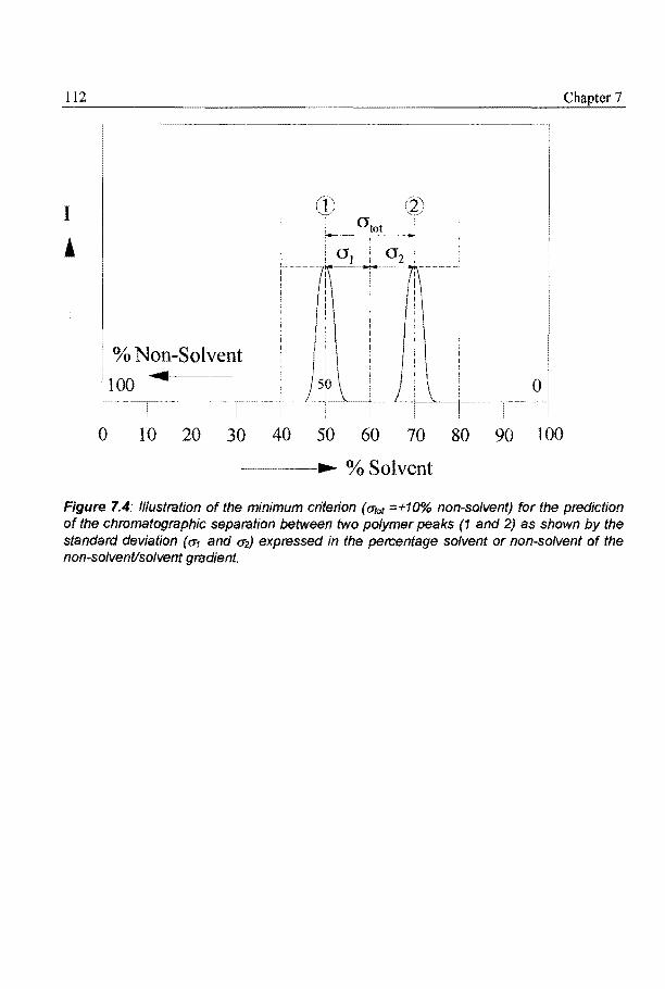
112
I
'
0
%Non-Solvent 100 .....
10 20 30 40 50 60
0
70 80 90 100
-----~~ % Solvent
7
Figure 7.4: Illustration of the minimum criterion (crtor =.±10% non-solvent) for the prediction of the chromatographic separation between two polymer peaks (1 and 2) as shown by the standard deviation ( cr1 and cr2) expressed in the percentage solvent or non-solvent of the non-so/vent/solvent gradient_

Prediction of Cloud-Points 113
7.2.7 The Conclusive Test
In order to test the predictive value of this direct method, the cloud-point observations presented in the publication of Suh and Clarke [9] were chosen. They applied 35 solvents to poly(styrene) (Appendix 23) that were not used in the present investigation. As calculation methods are chosen the most promising methods i.e., the method of Suh and Clarke and the direct method. The Hansen method is too inaccurate to calculate cloud-points for chromatographic applications.
The results of the calculations are shown in Table 7.5. The calculations are based on the coefficients of the calibration lines as shown in the Appendices 20 and 22. The results are better than expected from the calculations in the Sections 7.2.4 and 7.2.5. The reason for this satisfYing results may be that most solvents used for this test are chemically related such as the halogenated hydrocarbons which are good solvents. The standard deviation of the direct method is slightly better than the standard deviation of the method of Suh and Clarke.
The results (see Appendix 23) of the comparison between observed and calculated cloudpoints are presented in Figure 7.5 together with the calibration points and the trend lines of the Figures 7.2 and 7.3. The reason of the slightly higher standard deviation in the calculation method of Suh and Clarke is that the acetone non-solvent line shows a number of large deviations (right upper points ( 0) Figure 7.5 A). The reason for these large deviations is that the solubility parameter of acetone (6=20.1) is positioned between the solubility parameters of the solvents (see Appendix 23). As shown by Equation 7.2 when the difference in solubility parameter between solvent and non-solvent becomes too small the calculations results in infinitely large or small cloud-point values.
Table 7.5: Comparison between the Calculation Methods of Suh and Clarke and the Direct Method based on Test Solvents11 for Poly(styrene)21
Parameter
a( absolute)
% Predicted CPvalues without --· physical meaning
5l
1) Reference [9) 2) Molar mass L28xl06 g/mol 3) Using Eq 7.3 and Appendix 20 4) Using Eq 7.3 and Appendix 21 5) CP < 0 or CP > 100%
Suh and Clarke3lMethod
8
3
Direct Method4l
%NS 7
0

114 Chapter 7
10 20 3J 4J 50 00 70 80 00 100 (Cloud-Point ()bserved) "IoNS
100
00 co 80
~ 70 .. 1;j
00 ;; J:! ® I'll 50 (,)
i!
~ 4J
"C:: 30 .§ 2. 20
10
0 0 10 20 30 4J 50 00 70 80 00 100
(Cloud-Point Observed)o/.NS ------ ·········----
Figure 7.5: Test for the calculation methods of Suh and Clarke (A) and the direct calculation method (B), by a direct correlation between calculated and observed cloudpoints of poly(styrene) : <•J points used to calibrate the calculation methods (see Figure 7.4 and Appendices 20 and 21 ), (0) points to test the calculation methods (see Appendix 23).

Prediction of Cloud-Points 115
7.3 Conclusions
The prediction of the cloud-point of a polymer based on the solubility parameters of solvent, non-solvent and polymer is far from trivial. One problem is that for most polymers the solubility parameters are not known or can not be determined or calculated accurately. Even when the solubility parameters of a polymer are known, the relation between the solubility of the polymer and the solubility parameters ofthe liquids is rather poor (Table 7.2). The critical remarks of Van Krevelen in his book "Properties of Po{Ymers"[13) still apply today. "The mtai/able experimental data prove, however, that it is impossible to derive a simple system for an accurate prediction of solubility parameter components from the chemical structure. Especially the interaction of different structure groups in producing overall polar and hydrogen-bonding properties is so complicated that it does not obey simple rules. " This means that all existing calculation methods for the solubility parameter of the polymer do not result in more than rather rough estimates. These remarks are valid for the solubility of polymers in pure liquids. For the mixtures of liquids even larger deviations can be expected, because there are also specific solvent/non-solvent interactions possible.
The sphere of Hansen's calculation method is an interesting approach that works well for the prediction of polymer solubility in pure liquids and mixtures of liquids. This calculation method, however, is not accurate enough to predict the cloud-points. Deviations in the three solubility parameters (based on many different physical parameters) may be also the source of the poor quality of the prediction of the cloud-points.
The method of Suh and Clarke is more suited to the purpose of calculating cloud-points because the method is based on an indirect correlation between solubility parameters and cloud-points. The method gives better results than the Hansen method. A drawback of this method is that due to the way of calculating, a significant number of cloud-point values are calculated without physical meaning. This also leads to large deviations of the linear regression line to the theoretical line between observed and calculated cloud-points in the case of a small difference between the solubility parameter of solvent and non-solvent. Because of the interesting concept, future tests will be done to improve this method.
Another calculation method is suggested, based on the direct correlation between cloud-points and solvents used at constant non-solvent. This method gives the best overall quality for the prediction of the cloud-points of the three calculation methods.
As shown in Chapter 2, the rise of phase separation is a fragile combined action of enthalpy and entropy effects among polymer, solvent and non-solvent. Because of the complexity of these interactions, it is not possible to calculate the cloud-points directly from physical parameters like the energy of evaporation. Empirical relations between cloud-points and solubility parameters are needed, like the radius of interaction in the Hansen method, the correlation lines between omix and o• in the method of Suh and Clarke and the direct correlation

116 7
Jines between cloud-point and o", to calculate the cloud-point. A point of concern is that all these emperical correlations were rather poor.
The progress made in this investigation covers the comparison between the commonly applied Hansen method, the relatively unknown method of Suh and Clarke and the suggested direct method. The comparison clearly demonstrates the weakness of knowledge about the interactions between polymers and liquids as mentioned above, especially in the Hansen method. The methods of Suh and Clarke and the direct method are a great step forward, but they require too many experiments for a good prediction of the cloud-points.
Main future dev(;":lopments will be focused on improvements of the direct method, to obtain a better quality of the prediction of the cloud-point. One of the topics will be the study of the relation between homologous series of solvents and non-solvents, and cloud-points and solubility parameters. The aim of such a study is to calculate cloud-points directly from group contributions.

Prediction of Cloud-Points
7.4 References
[I] Hansen, C.M.J., Paint Technologies, 39, 104 (1967) [2] Shell, Technical Bulletin, ICS(x) 75/1. [3] Glockner, G., Chromatographia, 25, 854 (1988) [4] Schultz, R., Engelhardt, H., Chromatographia, 29,205 (1990) [5] Shalliker, R.A., Kavanagh, P.R.,J.Chromatogr., 543, 157 (1991) [6] Hildebrand, J.H., Scott, R.L., The Solubility ofNon-Electrolytes, Reinhold, N.Y
(1959). [7] Sub, KW., Corbett, J.M., J. Appl. polym. Sci, 12, 2359 (1967) [8] Burrell, H., Preprints, Division of Paint Plastics and Printing Ink. Chern. l27th ACS
Meeting, Cincinnati, (April1955)." [9] Sub, KW., Clarke, D.H., J. Polym. Sci, A-1, 5, 1671 (1967) [10] Hsieh, M.-M., Dorsey, J.G., J.Chromatogr., 631, 63 (1993) [Il] Scott, R.L., J. Chern. Phys., 17, 268 (1949) [12] Scott, R., P., W., Silica Gel and Bounded Phases, John Wiley and Sons, New York
(1993) [13] Van Krevelen, D.W., Properties of Polymers, Elsevier, Amsterdam (1990)
117

118

119
Epilogue
Introduction
Originally the scope of this thesis was very broad. The aim was to study and to solve the reported problems and unexplained phenomena reported in literature concerning gradient elution separation of polymers. During the research, it appeared that a large number of steps, based on different complex mechanisms, played a role in the separation process. The time available did not allow to thoroughly investigate the entire process. From the different mechanisms, the basic mechanism, i.e. the separation based on solubility, was chosen as subject for this thesis. The disadvantage of such a limitation is that many interesting observations could not be included. To complete the picture of the experimental work an overview is given below of achievements of this thesis and of other related results (beyond the scope of this thesis).
Achievements
Besides the chromatography, different chemical and physical properties of the standard polymers PB, PS and PMMA were studied. For example an overview is given of the solubility of this three polymers in pure (HPLC) solvents and of the solubility in solvent/non-solvent mixtures (cloud-points). Based on these cloud-points, information was obtained about the solvent and non-solvent strength (related to the polymer).
The chromatographic results can be divided in three sections, (1) the mechanism of separation of polymers, (2) the prediction of the separation behaviour, and (3) practical applications.
1) The mechanism
The most important discovery was that the separation of high molar mass polymers is dominated by a precipitation-redissolution mechanism. The validity of this mechanism was proven by the finding that a good correlation exists between titrimetrically and chromatographically obtained cloud-points.
2) The predictions
The aim of this investigation was to predict the cloud-points based on the Hildebrand and Hansen solubility parameters of solvents, non-solvents and polymers. Three different calculation methods have been compared in this study. The results of the first cloud-point prediction method based on the sphere of solubility calculation of Hansen, was very poor. The results of the second calculation method of Suh and Clarke were acceptable. The best results so far were obtained from a di~ect correlation between cloud-points and solubility parameters.

120
3) Practical Applications
One of the most valuable applications of GPEC is that it allows the prediction of the separation of polymer blends from titrimetrical cloud-point experiments. Another practical application of GPEC is the determination of the chemical composition of copolymers and the determination of minute differences in the polymer structure. The complete composition of a material i.e. residual monomer, additives, oligomers and polymers can be analysed. Differences in physical properties of the polymer can now be related to differences in polymer composition. It has been proven that for most THF and chloroform soluble polymers GPEC is a reliable chromatographic method that is relatively easy to apply.
Other related Results
The solubility of 11 other high molar mass commercially available THF soluble polymers was tested, applying the same 20 liquids used in the present investigation. An interesting correlation was obtained between polymer polarity and solvent polarity. Many cloud-points were determined on the basis of the results of this solubility experiments. Based on these cloud-point experiments many chromatographic experiments were performed. In nearly all cases a good correlation was obtained between the titrimetrically and chromatographically obtained cloud-points. The separation based on a precipitation-redissolution process seems to be the dominant mechanism.
In order to determine any possible adsorption of dissolved polymers on stationary phases in a fast and easy manner, a solid phase extraction test was developed (Sep-Pak test). With this test it was proven that the adsorption of dissolved high molar mass polymers on stationary phases was an exception. When poor solvents were used, however, adsorption of polymers was observed. Based on this test the solvents for the GPEC experiments were selected.
Much attention was given to the phenomenon of colloidal elution. At colloidal elution the polymer does not elute in a dissolved form, but as colloidal particles suspended in a nonsolvent. Besides size exclusion effects other important origins of this phenomenon were discovered. Cooling of the capillary between the column oven and the detector causes precipitation of the polymer, resulting in colloidal elution. In the past this phenomenon was unwanted because of a not reproducible responce of the polymer peak applying UV and fluorescence detectors. A better way to control this phenomenon was to add extra non-solvent after the separation. This phenomenon can now be used for detection of UV transparent polymers. This work resulted in a patent (Turbidity Detector Patent No. 942005620).
Future Outlook
Future research will be done on many chemical, physical and instrumental aspects of GPEC. Additional research may lead to the improvement of the quality of the predictions of the cloud-
121
points, based on the influence of the chemical structure of polymers and the influence of solvents and non-solvents. A very important subject for the future will be a study of the relation between the physical properties of the polymer and the chromatographically obtained solubility parameter distribution. Coupling of GPEC and GPC/SEC instruments (orthogonal chromatography) will extend the information about the polymer (MMCCD). Combining specific detectors that provide additional information on molar mass or chemical compositions with the GPEC separation, like light scattering (LALLS), viscometry, photodiode array (PDA) (UVIVIS detector), fluorescence detector (FL), infrared spectroscopy (IR), and nuclear magnetic resonance spectroscopy (NMR), will significantly contribute to the information gained from the separated polymer fractions.

122

Acknowledgements 123
Acknowledgements
The practical work set out in this dissertation was carried out at both the application laboratory of Waters Chromatography in Etten-Leur and the Polymer Chemistry Laboratory of Prof. A.L. German at Eindhoven University of Technology. First of all, the author would like to express his sincere gratitude to all those members of the Department of Polymer Chemistry who have helped contribute to this thesis. Thanks to Ton German, Alex van Herk, Bert Klumperman, Eric Nies and Henk Claessens for their helpful advice, guidance and encouragement. Particular thanks also to Wieb Kingma, Alfons Franken, Helly van der Heyden and Ruud Monten for logistical organisation. Special thanks also go to the graduate students who have enthusiastically assisted on this project: Paul Cools, Rob Hilgers Christan Luijkx, Tonnie Willems, Maarten de Klerk and Harold Kuijten. The 'Brouwershaven meeting', the 'Lieshout wood party' and the 'Dwingelo meeting' made a particularly lasting impression on me. Thanks to Hans Frank and Hugo Billiet of Delft University of Technology for the HPLC comments.
Grateful thanks go to Waters former Managing Director Ton van de Put, who saw the firm through 'thick and thin', and without whose support this project would never have come to fruition. In addition, to Marcel De Valek, initially in a lesser role, now at the fore in his job as Waters Benelux manager. Thanks also to Pim de Swart for the excellent 'Excel programme' and colleagues Ronald Haas, Fred Ploeg, Chris Mol, Ad Hagenaars, office staff Ankie van de Wijngaart, Ghislaine Dellepoort and Ellen Brouwers for their interest and support. Also, thanks to Richard Payne, Andre Ayache and Gerard Bondoux of Waters European Headquarters in France for their financial support, to the American Headquarters of Waters Chromatography, especially John Morawski who was able to 'conjure up' funding and technical apparatus from all over the place, to Rick Nielson for pointers for my publications, to Brian Murphy for a number of text amendments, and to Bob Pfeiffer, Gary Fallick and Mark Andrews for financial support with this thesis and Bill Dark for promoting GPEC® in Milford.
There are several people to whom I owe special thanks: firstly to Jan Jansen of Philips in Eindhoven who helped set me on track in this endeavour and to Gottfried Glockner who shared his great expertise and knowledge of this subject with the author. Thanks to Jaap Brasser, Cees Evers and Yi.iksel Sahin of General Electric ABS in Amsterdam for their contribution to the 'Chromatograms of Standards'. Thanks also to Maarten Zonneveld of Akzo Nobel in Sassenheim for his help with the solubility parameters.
Further acknowledgements go to the enjoyable collaboration with English language editor Michael Tait of Etten-Leur for his valuable inputs and comments and to Steven Ralston the English language editor of Eindhoven University of Technology for his enthusiastic lessons.
Finally, I am very grateful to have found a worthy successor in Harry Philipsen from Oce in Venlo. I wish him every success i~1 the continuation of this work.

124

Curriculum Vitae 125
Curriculum Vitae
The author of this thesis, Wim Staal, was born on 7 September 1948 in Bergen op Zoom, the Netherlands. In 1965 he received the Mulo-A diploma with Mathematics (first certificate in secondary education) at the Parochial Christian Secondary School, Bolwerk Str. Bergen op Zoom (now closed). A year later in 1966 he became the first pupil in his school to receive a Mulo-B diploma with chemistry. In that extra year he enjoyed an 'explosive' time as a lab assistant. This was followed by two years studying chemical engineering at Dordrecht College of Advanced Technology (HTS). Because his main interest was in chemistry rather than in engineering he decided to switch to the course in analytical chemistry in Breda. However, this change-over meant that he was first required to do his military service. It was for this reason that it took until 1971 to finally attain the First Higher Vocational Diploma (HBO-A) in analytical chemistry by attending classes at night school in Breda. Continuing his studies he also completed the Second Higher Vocational Diploma (HBO-B) in 1973 and went on to earn a diploma in chemistry at the Advanced School of Technology (HTS) in Rotterdam. His major subject during his graduation course was the pyrolysis-gas chromatography of polymers, reflecting his interest in polymer technology research. After this he followed various courses including a teaching course in Goes, the SBB environmental course in Utrecht and he completed an examination in macromolecular chemistry at the University of Antwerp (UIA) in 1977.
In 1971 he worked at the analysis laboratory of the Liga Biscuit Factory in Roosendaal for six months. Due to the attractive research in organoleptic competition, i.e. biscuits-tasting and testing, he put on quite a bit of weight.
Something which seemed much more of a challenge was working at General Electric Plastics in Bergen op Zoom. He worked in the quality control department, the analytical laboratory and the process development department from 1971 to 1977. All of this under the inspiring guidance of Prof. J. Bussink. This period was an excellent opportunity to learn more about American working practices and business philosophy.
In 1977 he moved to a job where he had a greater degree of autonomy and variety of tasks at the sales laboratory ofWaters Chromatography in Etten-Leur. From 1977 up to the present he has studied many aspects of liquid chromatography with regard to polymer research. Former managing director and mentor A. van ·de Put attempted to refine the commercial instincts of this 'research man'.

126 Curriculum Vitae
In 1988 he successfully reproduced the work set out in a publication by Prof G. Glockner (Dresden). This later turned out to become the basis for this thesis. The work was subsequently successfully tested on practical samples with Dr. J. Jansen of the Philips Research Laboratories in Eindhoven. In attempting to give this project a proper theoretical foundation, advice was sought from Prof. A.L. German and Prof C. A.M. G. Cramers at Eindhoven University of Technology. This collaboration led to greater insight, various publications and a lot of useful contacts, domestic as well as and abroad. During this period he was able to get a taste of the more relaxed and more informal way of working in the academic world.
He has written a variety of papers in the area of environmental chemistry, gel permeation chromatography (GPC), and in the area of polymer separation through gradient elution liquid chromatography (GPEC). He has presented several lectures on these topics at various national and international symposia. In addition, he is also the founder and chairman of the gel permeation chromatography users group (a division of the analytical separation methods section ofthe Royal Dutch Chemical Society (KNCV).

Appendix 127
Appendix 1: Suppliers of HPLC Solvents
Solvent Su~~lier Qualit,r 1 2,2, 4-Trimethylpentane Baker PA 2 Diethyl ether BDH PA 3 Cyclohexane Merck PA :,
4 Tetra chloromethane Baker PA 5 Toluene Rathburn PA 6 Dichloromethane Mallinckrodt HPLC 7 Chloroform Rathburn HPLC 8 Tetrahydrofuran Westburg HPLC 9 1,4-Dioxane Baker PA 10 N,N -Dimethylacetamide Dupont PA 11 N,N-Dimethylformamide Baker PA 12 Benzyl alcohol Merck PA 13 Methyl ~thy! ketone Merck PA 14 Ethyl acetate UCB PA 15 Dimethyl sulfoxide Baker PA 16 Acetone Westburg PA 17 Acetonitrile Westburg HPLC 18 2-Propanol BDH PA 19 Methanol Rathburn HPLC 20 Water Milli-Q Millieore HPLC

128
Appendix 2: Structure of HPlC Solvents
2,2, 4-Trimethylpentane
2 Diethyl ether
3 Cyclohexane
4 Tetrachloromethane
5 Toluene
6 Dichloromethane
7 Chloroform
8 Tetrahydrofuran
9 I ,4-Dioxane
I 0 N,N-Dimethylacetamide
CH3
I CH3-C CH3
I CH2
I CH-CH3
I CH3
~H5~0-~Hs
H2f~rHz H2C. /CHz
CH2
CC4
Q-a~ C~Clz
CliC13
H2T-Tfb
fuc_,_ /Cfb 0
/0'-._
Hzy TH2
H2c_,_ /CH2 0
?i /CH3 CH3-C-N
'cH3

Appendix 2: Continued
Solvent II N,N-Dimethylformamide
I2 Benzyl alcohol
13 Methyl ethyl ketone
14 Ethyl acetate
15 Acetone
I6 Dimethyl sulfoxide
17 Acetonitrile
18 2-Propanol
19 Methanol
20 Water
Structure
CH3-~-CzHs 0 II
CH3-C-0-C2Hs
CH3-~-cH3 CH3
O=S.I -
' CH3
CH_,-O"==N
OH
CH:J~H-CH3 CH_,-OH
H20
I29

130 Appendix
Appendix 3: Solubility Parameters of HPLC Solvents
Solvent Solubilit_y Parameters (MPat2
0d 0 oh Ot
2,2, 4-Trimethylpentane 14.3 0 0 14.3 2 Diethyl ether 14.5 2.9 5.1 15.8 3 Cyclohexane 16.8 0 0.2 16.8 4 Tetrachloromethane 17.8 0 0.6 17.8 5 Toluene 18.0 1.4 2.0 18.2 6 Ethyl acetate 15.8 5.3 7.2 18.2 7 Chloroform 17.8 3.1 5.7 19.0 8 Methyl ethyl ketone 16.0 9.0 5.1 19.0 9 Tetrahydrofuran 16.8 5.7 8.0 19.4 10 Acetone 15.5 10.4 7.0 20.1 11 Dichloromethane 18.2 6.3 6.1 20.3 12 1,4-Dioxane 19.0 1.8 7.4 20.5 13 N,N-Dimethylacetamide 16.8 11.5 10.2 22.7 14 2-Propanol 15.8 6.1 16.4 23.5 15 Benzyl alcohol 18.4 6.3 13.7 23.7 16 Acetonitrile 15.3 18.0 6.1 24.6 17 N,N-Dimethylformamide 17.4 13.7 11.3 24.8 18 Dimethyl sulfoxide 18.4 16.4 10.2 26.7 19 Methanol 15.1 12.3 22.3 29.6 20 Water 15.6 16.0 42.4 47.8
l) Hansen solubility parameters, Polymer Handbook, References 4.4 [2)

,.... M
Appendix 4: Physical Properties of HPLC Solvents 11
Solvent Melting Boiling Refractive Viscosity uv Dielectric Miscibilicyl> Point Point Index [cP 20°C] cut-off Constant Number [oC] eq [20°C] [nm] [M]
1 2,2, 4-Trimethyl-pentane -107 99 1.3910 0.50 215 1.9 29 2 Diethyl ether -116 34.6 1.3530 0.23 215 4.3 23 3 Cyclohexane 6.5 81 1.4260 1.00 200 2.0 28 4 T etrachloromethane -32 77 1.4595 0.97 263 2.2 5 Toluene -93 111 1.4960 0.59 285 2.4 23 6 Dichloromethane -97 40 1.4240 0.44 235 9.0 20 7 Chloroform -63 61 1.4460 0.57 245 4.8 19 8 Tetrahydrofuran -108 67 1.4070 0.55 215 7.6 17 9 1 ,4-Dioxane 11.8 101 1.4220 1.54 215 2.2 17 10 N ,N -Dimethyl-acetamide -20 165 1.4380 268 11 N,N-Dimethyl-formamide -61 153 1.4310 0.92 268 12 12 Benzyl alcohol -15.3 205 1.5396 285 17 13 ~ethyl etl1ylketone -86.4 79.6 1.3788 0.40 330 18.5 14 Etllyl acetate -84 77 1.3720 0.45 260 6.0 19 15 Dimethyl sulfoxide 18.4 189 1.4770 2.24 268 4.7 9 16 Acetone -94 56 1.3590 0.32 330 21.4 15, 17 17 Acetonitrile -48 82 1.3440 0.37 190 37.5 11, 17 18 2-Propanol -89.5 82.4 1.3770 2.30 210 20.3 15 19 Methanol -98 64.6 1.3290 0.60 205 32.7 12 20 Water 0 100 1.3330 1.00 <190 80
I) Gant, R., LC-GC Int., 5, 9, 25 (1992) 2) All pairs whose M number differs by 15 units or less are miscible in all proportions at 15 oc
.~ Each pair whose M number differs by 16 has a critical solution temperature between "0 25 °C and 75 °C, approximately 50 °C preferably. A difference of 17 or more corresponds to 1:: <!,) immiscibility or to a critical solution temperature above 75 oc P..
~

132
Appendix 5: Experimentally Determined Miscibility of HPLC Solvents11
Solvent 1 2 3 4
1 03)
2 0
3 0
4 0
5 6 7 8 9 10 11 12 13 14 -15 -16 - -17 - -18 - -19 - -20 - - - -
1 2,2, 4-Trimethylpentane 2 Cyclohexane 3 Tetrachloromethane 4 Toluene 5 Dichloromethane 6 Chloroform 7 Diethyl ether 8 Methyl ethyl ketone 9 Ethyl acetate 1 0 T etrahydrofuran
5 6
0
0
- -
7 8 9
0
0
0
- - -
10 11 12 13 14 2) -
0
0
0
0
0
-
11 Acetone 12 2-Propanol 13 1,4-Dioxane 14 Benzyl alcohol
15 16
- --
0
0
15 N,N-Dimethylacetamide 16 N,N-Dimethylformamide 1 7 Dimethyl sulfoxide 18 Acetonitrile 19 Methanol 20 Water
l) Mh:ture of 50/50 v/v at 20°C, no value is miscible 2) • = Immiscible 3) o = The same liquids
17 18 19 20
- - - -- - - -
-------
-
0
0
0
0

133
Appendix 6: Experimentally Determined Miscibility of HPLC Solvents11
Solvent vol. o/o Solvent vol. o/o Water in 2,2,4-Trimethylpentane <1 2,2, 4-Trimethylpentane in water <1 Water in Cyclohexane <I Cyclohexane in water <I Water in Tetrachloromethane <I Tetrachloromethane in water <I Water in Toluene <I Toluene in water <I Water in Dichloromethane <I Dichloromethane in water <I Water in Chloroform <1 Chloroform in water <I Water in Diethyl ether 1.3 Diethyl ether in water 7.9 Water in Ethyl acetate 3.0 Ethyl acetate in water 6.9 Water in Benzyl alcohol 10 Benzyl alcohol in water 5.8 Water in Methyl ethyl ketone ·11 Methyl ethyl ketone in water 32 Methanol in 2,2,4-Trimethylpentane <I 2,2, 4-Trimethylpentane in Methanol 3.8 Methanol in Cyclohexane <I Cyclohexane in Methanol <1 Acetonitrile in 2,2, 4- <I 2,2, 4-Trimethylpentane in Acetonitrile 4.8 Trimethylpentane Acetonitrile in Cyclohexane <1 Cyclohexane in Acetonitrile 4.8 Dimethyl sulfoxide in 2,2,4- <1 2,2,4-Trimethylpentane in Dimethyl <1 Trimethylpentane sulfoxide Dimethyl sulfoxide in Cyclohexane 2.4 Cyclohexane in Dimethyl sulfoxide 2.4 N,N-Dimethylformamide in 2,2,4- <I 2,2,4-Trimethylpentane in N,N- <1 Trimethylpentane Dimethylformamide N,N-Dimethylformamide in 30 Cyclohexane in N,N- 2.5 Cyclohexane Dimethylformamide N,N-Dimethylacetamide in 2,2,4- 40 2,2, 4-T rimethylpentane in N ,N- <I Trimethylpentane Dimethylacetamide Benzyl alcohol in 2,2,4- 20 2,2, 4-Trimethylpentane in Benzyl <I Trimethylpentane alcohol
1) At 20 oc

134 Appendix
Appendix 7: Data of Poly(butadiene) Standards11
Molar Mass of Poii:{butadiene} Standards in 2/mol Batch No. IV21£dllg] Mv Mn Mw M~ Mw/Mn 21323-1 0.039 893 838 907 893 1.08 21326-3 0.088 2,820 2,879 2,966 3,002 1.03 21328-2 0.181 7,848 7,848 8,042 7,970 1.03 21329-1 0.214 9,952 9,176 9,411 9,320 1.03 21332-2 1.479 31,200 31,420 32,030 31,400 1.02 21334-2 0.924 79,250 78,800 80,610 80,410 1.03 21335-1 1.165 11,090 118,100 120,800 120,000 1.03 21338-1 2.551 334,600 304,700 316,300 329,100 1.04 21339-1 3.452 513,900 485,700 500,000 491,400 1.03 21341-1 5.562 1,011,000 941,100 966,900 952,800 1.03
1) Manufactured by Polymer Laboratories (U.K.) 2) Intrinsic viscosity in tolue:ne at 30°C, K = 0.000325 (dl/g), alpha= 0.705 (range molar mass
7,000 -1,000,000 g/mol)
Polymerization
Poly(butadiene) is produced by anionic polymerization initiated with n-butyllithium and terminated with methanol. These polymers contain residual double bonds, are unstable after a time and require storage in a refrigerator under inert gas. The cis/trans ratio is 1.1-1.2 and the viny11.2 content is 5.3-7.6% CHNMR and 13C NMR).

Appendix 135
Appendix 8: Data of Poly( styrene) Standards 1,
Molar Mass of Pol!{ styrene} Standards in g/mol Batch NMR Osmometry Viscometry2> LS6)
No. Mn Mn IV [dllg] Mv Mw 20122-9 542 561 4
) + 20124-6 1,235 1,2104
) 1,440 20126-6 3,050 3,2004
) 0.0468 3,1903) 3,275
20129-3 + + 0.0913 9,7003) 10,100
20132-3 + 26,8905) 0.179 29,500 28,720 20134-4 + 61,2005) 0.304 62,100 66,000 20137-6 + 153 6005) 0.591 158,800 162,000
' 20139-12 + + 1.243 452,200 493,000 20142-3 + + 2.566 1,255,000 1,280,000 20145-10 + + 4.608 2,863,000 3,200,000
Batch GPC/SEC No. Mn Mw M~ Mw/Mn 20122-9 565 653 580 1.16 20124-6 1,224 1,303 1,319 1.07 20126-6 3,091 3,212 3,252 1.04 20129-3 9,661 9,910 10,110 1.03 20132-3 2,7570 28,580 28,520 1.03 20134-4 64,570 66,440 66,000 1.03 20137-6 152,400 456,100 156,500 1.03 20139-12 460,100 491,100 500,800 1.06 20142-3 1,208,000 1,281,000 1,291,000 1.06 20145-10 2,899,000 3,055,000 3,149,000 1.06
+ Technique not applicable 1) Manufactured by Polymer Laboratories (U.K.) 2) Intrinsic viscosity in toluene at 30°C, K"" 0.00021 (dl/gr) alpha= 0.71 (range molar mass 20,000-
20,000,000 g/mol) 3) K = 0.00037 (dl/g) alpha= 0.6 (range molar mass 1,000-20,000 g/mol) 4) Vapour Phase Osmometry 5) Membrane Osmometry 6) Light Scattering
Polymerization
The poly(styrene) standards are produced by an amomc polymerization process. The polymerization is initiated with n-buty1lithium and terminated with alcohol. This produces end groups ofn-buty1 and methyl. Poly( styrene) produced under these conditions is atactic.

136 Appendix
Appendix 9: Data of Poly( methyl methacrylate) Standards 11
Molar Mass of Poly(methii methacrylate) Standards in g/mol Batch Viscometry GPC/SEC No. IV[dllg] Mv Mn Mw M~ MwfMn 20222-1 0.01792) + 603 735 625 1.22 20226-5 0.0406 + 3,437 3,673 3,805 1.07 20228-4 0.0524 6,856 6,876 7,248 7,611 1.06 202304 0.0801 13,040 12,490 13,530 13,930 1.06 20321-6 0.1125 21,800 23,240 24,580 24,280 1.06 20234-6 0.2212 60,780 60,200 63,650 62,590 1.06 20236-2 0.4028 150,700 148,300 153,500 153,700 1.04 20238-5 0.6654 322,400 311,700 330,100 333,000 1.06 20240-5 1.0480 675,400 623,200 685,500 684,8008 1.10 202424 1.6660 1,295,000 1,222,000 1,295,000 1,286,000 1.06
+ Technique not applicable I) Manufactured by Polymer Laboratories (U.K.) 2) Intrinsic viscosity in toJuene at 25°C, K 0.000154 (dllg) alpha= 0.66 (range molar mass 5,000-
1,500,000 glmol)
Polymerization
The low molar mass polymers (<15,000 glmol) are made by group transfer polymerization, so the polymer has no additional end groups other than the repeat unit. The high molar mass polymers are obtained by anionic polymerization using cumyllithlum as an initiator and terminated with methanol. The polymers made in this way, using polar solvents and low
, temperature ( -100 oq are approximately 2-5% isotactic, 50-60% syndiotactic and 20-45% atactic.

Appendix 137
Appendix 10: Structure of Polymers
1 1, 4-Poly(butadiene) H H I I (PB)
-(-C~-C=C-C~-in
1 ,2-Poly(butadiene) Cllj--CH--Jn (PB)
I CH
II c~
2 Poly( styrene) "f-CH,6!B; (PS)
,~
.,Q
3 Poly( methyl TH3 methacrylate) -t-CH2-T--1n (PMMA)
r=O
~H3

138 Appendix
Appendix 11: Published Cloud-point Values of Poly( styrene)
Comparison of Cloud-Point Observations of Poly( styrene) between Present Investigation and Published Values
Source Non-Solvent Solvent Temperature (%] [%) (%] [OC]
Methanol T etrachloromethane Observation1> 21 79 Ambient Literature [2tfl 20 -1 80 25 Literature [14]3
) 18 -3 82 25 Methanol Chloroform
Observation 27 73 Ambient Literature (14] Jl 25 -2 75 25 Literature (21] 2l 27 0 73 25
Methanol Toluene Observation 23 77 Ambient Literature (21) 2J 25 +2 75 25 Literature [16] 20 -3 80 25
Methanol Methyl ethyl ketone Observation 12 88 Ambient Literature [14] 3l 11 -1 89 30
Methanol Dichloromethane Observation 26 74 Ambient Literature [21] 2J 22 -4 78 25 Literature [23fl 28 +2 72 25 Literature (26t> 30 +4 70 35
Methanol Tetrahydrofuran Observation 40 60 Ambient Literature [14] 3J 29 -11 71 25 Literature (25]'l 40 0 60 20
Methanol 1,4-Dioxane Observation 28 72 Ambient Literature (14] 3J 29 +1 71 25
Acetone Toluene Observation 85 15 Ambient Literature [21] 2J 86 +1 14 25
Acetone T etrachlorornethane Observation 83 17 Ambient Literature [21] 2
) 93 +10 7 25 Acetone Chloroform
Observation 76 24 Ambient Literature (21] 2
J 79 +3 21 25
Acetone Dichloromethane Observation 71 29 Ambient Literature (21] 2
) 73 +2 27 25

Appendix 11: Continued
2-Propanol 1 ,4-Dioxane Observation 44 56 Literature 115] 45 +1 55
Water T etrahydrofuran Observation 10 90 Literature [17]4
J 9 -1 91 Acetonitrile Dicholoromethane
Observation 46 54 Literature [24]6
J 47 +1 53 2,2, 4-Trimethylpentane Toluene
Observation 49 51 Literature [21] 2
) 52 +3 48 2,2, 4-Trimethylpentane
Observation 55 45
l) Present investigation molar mass 1,280,000 g/mol, cone. l mg/ml Table 5.4 2) Poly( styrene) molar mass 295,000 g/mol, cone. 3 mg/ml 3) Molar mass 335,000 g/mol, cone. l mg/ml 4) Molar mass l.2xl06 g/mol, cone. l mg/ml 5) Molar mass 929,000 g/mol, cone. 0.2 mg/ml 6) Molar mass 929,000 g/mol. cone. 0.2 mg/ml 7) Molar mass 106 g/mol, cone. 0.04 mg/ml 8) Molar mass 106 g/mol, cone. 0.04 mg/ml 9) CP difference between literature and present investigation For literature see References 5.4
Ambient 20
Ambient 25
Ambient 35
Ambient 25
Ambient
Determination of the Standard Deviation of the Cloud-Point of Poly(styrene)11 in the THF-Methanol System
Observation number I 2 3 4 5 6 7 8 9 10
Average
1) Molar mass 1,280,000 g/mol 2) Ambient temperature
Cloud-Point % Methanofl 39.8 40.2 40.2 39.1 40.5 40.2 40.5 40.2 40.2 39.5 40.0
139

140
Appendix 12: Published Cloud-point Values of Poly( methyl methacrylate)
Comparison of Cloud..Point Observations of Poly( methyl methacrylate) between Present Investigation and Published Values11
Source Non-Solvent Solvent Temperature [%] [%) (o/o] roq
Water 1,4-Dioxane Observation 18 82 25 Literature [18] 15 +3 85
Methanol Toluene Observation 66 34 26.2 Literature [19] 64 +2 36
Cyclohexane 1,4-Dioxane Observation 49 51 25 Literature (22]2
l 47 +2 53 Cyclohexane Toluene
Observation 30 70 25 Literature (21] 33 +3 67
Methanol Tetrachloromethane Observation 65 35 25 Literature [22] 2
) 47 +18 53 Methanol Acetone
Observation 61 39 25 Literature [22) 2l 22 +39 78
l) Present investigation, molar mass 1,300,000 g/mol, cone. 1 mg/ml 2) CP difference between literature and present investigation
For literature see References 5.4

Appendix 141
Appendix 13: Solubility Parameters of the Three Standard Polymers 11
Solubility Parameters (MPai'2
Polymer od 0 oh Ot RAo Poly(butadiene) 17.53 2.25 3.42 18.0 6.5 Poly( styrene) 21.28 5.75 4.30 22.47 12.7 Poly(methyl methacrylate) 18.64 10.52 7.51 22.69 8.6
1) Hansen solubility parameters, Polymer Handbook, References 4.4 121

142
Appendix 14: Molar Mass Dependency of the Cloud-Point11 at Ambient Temperature
Molar Mass Dependency of Poly(styrene), Poly(butadiene) and Poly(methyl methacrylate) Related to the Cloud-Point in Water- Tetrahydrofuran and 2,2,4-Trimethylpentane- Tetrahydrofuran
Polymer Molar Mass Cloud-Point:% Water Cloud-Point: % 2,2,4-Trimethylpentane
Poly(butadiene) 950,000 5.8 100.0 330,000 5.8 120,000 6.3 80,000 6.6 21,000 6.7
3,000 14.5 900 29.3
Poly( styrene) 20,600,000 9.5
3,150,000 9.9 55.0 2,700,000 9.9 1,290,000 9.9 55.8
500,800 10.7 57.6 156,000 11.5 59.3 96,400 12.1 66,000 13.0 65.0 28,500 14.5 72.1 10,100 20.0 85.1 3,250 29.1 100.0 1,320 39.8
580 48.5
Poly(methyl methacrylate) 1,300,000 23.7 30.6
685,000 24.8 30.1 330,000 26.4 30.6 153,700 26.5 31.5 62,600 28.6 32.0 24,300 34.2 42.9 13,900 38.2 47.6 7,600 42.5 58.3 3,800 50.0 71.4
625 78.3 100.0 I) Polymer cone. 1 mg/ml

143
Appendix 14 Continued
30.
25
ii:' 20 ~ ...
15 -.$ • I'C :=
10 ~ 0
5
0
0 2 5 6
60.
50
ii:' 40 • ~ ...
30 I 20 '*
• •
10 .
0 0 2 3 4
log Molar Mass
80
70
60.
5 50 1::' .$ 40 . I'C := 30 ~ .,.
20
10
0 -
0 2 3 4 5 6 7 log Molar Mass

144
Appendix 14 Continued
80
ii:' u 60 0: ~ 40 '#.
20
0
0 1
2 3 4 5 log Molar Mass
2 3 4 5 log Molar Mass
6 7
6 7

145
Appendix 15: Influence of the Polymer Concentration on the Cloud..Point
Experimentally Determined Influence of the Polymer Concentration on the Cloud-Point of the System Tetrahydrofuran-Water for Poly(styrene) at different Molar Mass at 23.5°C
Molar Mass g/mol
1,090,000
96,000
18,100
580
Concentration mg/ml
0.13
1.20 11.51
0.10 1.02 10.20
0.10 1.28
10.96
0.10 4.50
Cloud-Point log %water
-0.886 10.7
0.079 9.9 1.06 9.8
-1.00 13.2 0.009 12.1 1.009 10.8
-1.00 19.4 0.107 16.6 1.040 13.4
-1 51.0 0.65 40.8
36.7
....... --··~~~~~···········-~ -~~~-···········~·~-- ···-~-'-,
-2 -1 0 1 log Cone. (mg/ml)
2
• 1,090,000 g/mol
• 96,000 g/mol
18,100 g/mol
580 g/mol

146
Appendix 16: Influence of the Temperature on the Cloud-Point.
Experimentally Determined Influence of the Temperature on the Cloud-point of the Tetrahydrofuran-Water System for Poly(styrene) at Different Molar Mass
Tem2erature Molar Mass Poli:(sti:rene) oc 500 g/mol 18, I 00 g/mol I 02,000 g/mol
%water 0 Il.l
10 47.3 15.6 11.7
24 50.8 16.6 11.9
30 51.4 16.6 12.0
40
1) Cloud-point e;,:presscd in %water, polymer cone. 1 mg/ml
50 • •
0 10 20 30
Temperature ('C)
---------------·
• 18,100 g/mol , ! • 102,000 g/mol I
l)(_~~~o, ooo g/m~lj
40
2,880,000 g/mol %water
9.5
9.7
9.9
10.0
1 1

147
Appendix 17: Cloud-Points of Poly(butadiene)11 Transformed in the Solubility Parameter o:ix
Solvent 1 2 3 6 4 5 7 8
() 14.3 15.8 16.8 20.3 17.8 18.2 19 19.4 2,2,4-Trimethylpentane 14.3
2 Diethyl ether 15.8 3 Cyclohexane 16.8 4 Tetrachloromethane 17.8 5 Toluene 18.2 6 Dichloromethane 20.3 7 Chloroform 19.0 8 Tetrahydrofuran 19.4 9 1 ,4-Dioxane 20.5 20.3 10 Ethyl acetate 18.2 17.02
) 17.9 18.9 18.1 18.2 18.4 18.4 11 Methyl ethyl ketone 19.0 17.3 18.5 19.4 18.7 18.8 19.0 19.1 12 Benzyl alcohol 23.7 19.0 19.4 22.4 20.4 20.6 21.6 21.4 13 Acetone 20.1 16.8 18.4 20.2 18.9 19.1 19.5 19.7 14 N,N-Dimethylacetamide 22.7 18.4 18.0 21.2 19.8 20.0 20.6 21.0 15 2-Propanol 23 5 16.6 18.9 21.6 19.9 20.1 21.0 21.2 16 N,N-Dimethylformamide 24.8 18.0 21.6 20.0 20.3 21.0 21.5 17 Acetonitrile 24.6 16.6 21.2 19.4 19.9 20.6 20.7 18 Dimethyl sulfoxide 26.7 17.1 21.5 19.5 20.1 21.0 21.2 19 Methanol 29.6 16.5 22.1 19,8 20.4 21.4 22.0 20 Water 47.8 21.1
Average value 8:ix 19.7 (Mpa)112
1) Cloud-point values see Table 5.1
2) a:ix in (MPa) 112 (Eq 2.18)

148
Appendix 18: Cloud~Points of Poly(styrene)11 Transformed in the Solubility Parameters 8mix and 8mix
np po
Solvent
0 1 2,2,4-Trimethylpentane 14.3
2 Diethyl ether 15.8
3 Cyclohexane 16.8
4 T etrachloromethane 17.8
5 Toluene 18.2
6 Dichloromethane 20.3
7 Chloroform 19.0
8 Tetrahydrofuran 19.4
9 1,4-Dioxane 20.5
10 N,N~Dimethylacetamide 22.7
11 N,N-Dimethylformamide 24.8
12 Benzyl alcohol 23.7
13 Methyl ethyl ketone 19.0
14 Ethyl acetate 18.2
l 5 Acetone 20.1
16 Dimethyl sulfoxide 26.7
l 7 Acetonitrile 24.6
1 8 2-Propanol 23.5
19 Methanol 29.6
20 Water 47.8
(A) Average value 8;" 16.5 (MPa)112
-mix (B) Average value 8po 22.0 (MPa)112
l) Cloud-point values see Table 5.4 2) 8mix in (MPaf2 (Eq 2.18)
3
16.8
4 5 6 7 8 9 10 11 12 13 14
17.8 18.2 20.3 19.0 19.4 20.5 22.7 24.8 23.7 19.0 18.2
16.3 16.3 16.3 15.9 17.4 17.4 - - 17.2 16.8 !A 16.1 16.0 16.4 16.2 16.6 16.7 - 17.6 - 16.3 16.3
19.72) 19.8 20.2 19.8 20.0 20.2 20.6 21.3 20.6 19.6 19.1 1
22.3 22.6 23.8 24.3 24.o 23.o 24.9 25.7 2s.o 23.4 21.9 I 20.8 21.6 22.3 21.9 22.2 22.0 23.3 24.8 24.1 20.1 19.0 ~ J
19.6 t9.9 21.1 20.9 21.4 2L8 23.1 24.3 23.7 19.8 t9.I I 20.3 2o.8 22.1 21.9 23.5 23.o 2s.1 25.8 24.7 20.3 19.1 I
- 22.2 22.1 23.7 25.3 - - J

149
Appendix 19: Cloud-Points of Poly(methyl methacrylate) Transformed in the Solubility Parameters /)mix and /)mix
np po
Solvent 0
2,2,4-Trimethylpentane 14.3
2 Diethyl ether 15.8
3 Cyclohexane 16.8
4 Tetrachloromethane 17.8
5 Toluene 18.2
6 Dichloromethane 20.3
7 Chloroform 19.0
8 Tetrahydrofuran 19.4
9 1 ,4-Dioxane 20.5
10 N,N-Dimethylacetamide 22.7 1 I N,N-Dimethylformamide 24.8
12 Benzyl alcohol 23.7
13 Methyl ethyl ketone 19.0
14 Ethyl acetate 18.2
15 Acetone 20.1
16 Dimethyl sulfoxide 26.7
17 Acetonitrile 24.6
18 2-Propanol 23.5
19 Methanol 29.6
20 Water 47.8
-mix (A) Average value li np 17.3 (MPa)112
-mix (B) Average value /ipo == 25.2 (MPa)112
1) Cloud-point values see Table 5.7 2) o'""' in (MPa)112 (Eq 2.18)
4 5 6 7 11 16 12 17 10 9 13 15 8 14 17.8 18.2 20.3 19.0 24.8 26.7 23.7 24.6 22.7 20.5 19.0 20.1 19.4 18.2
17.6 17.4 16.9 16.0 - - 18.2 17.5 18.1 17.9 11.1 1 17.7 17.8 17.9 17.3 - - 20.0 - 20.0 18.7 18.0 18.4 18.4 17.6 ~A
17.2 17.0 16.7 16.6 17.6 19.3 17.4 18.7 17.2 17.0 16.8 17.2 17.2 16.7 J
21.22) 21.6 22.9 23.1 23.8 24.1 23.5 23.7 23.3 22.7 21.8 22.4 21.9 21.3 l
25.5 25.7 27.5 27.5 28.4 29.0 28.5 27.9 27.9 27.5 25.8 25.9 26.2 24.9 ~B
- 26.9 28.6 - 28.1 26.5 25.4 - 24.5 26.2 - J

150
Appendix 20: Coefficients of omix Lines at Constant Non-Solvent using the Suh and Clarke Method11
Pol;r(butadiene} 8"'ix = a8' + b a b
Ethyl acetate 0.36 11.54 0.184 Methyl ethyl ketone 0.41 11.23 0.246 Benzyl alcohol 0.78 6.49 0.220 Acetone 0.10 6.19 0.320 N,N-Dimethylacetamide 0.66 7.99 0.123 2-Propanol 1.07 0.36 0.528 N,N-Dimethylformamide 0.85 4.69 0.267 Acetonitrile 1.04 0.54 0.425 Dimethyl sulfoxide 1.17 -1.39 0.120 Methanol 1.52 -7.49 0.151
Pol;r{ styrene} 2,2,4-Trimethylpentane 0.19 13.02 0.495 Diethyl ether 0.22 12.12 0.122 Acetone 0.21 15.88 0.146 Dimethyl sulfoxide 0.47 14.02 0.481 Acetonitrile 0.62 9.36 0.825 2-Propanol 0.75 6.14 0.472 Methanol 0.84 5.46 0.965 Water 0.60 10.30 0.409
Pol;r{meth;r:I methacrylate} 2,2, 4-Trimethylpentane 0.34 11.16 0.195 Cyclohexane 0.44 9.80 0.176 Diethyl ether 0.22 12.69 0.467 2-Propanol 0.33 15.56 0.283 Methanol 0.40 18.56 0.659 Water 0.44 16.53 0.769
1) References 7.4 [9]

151
Appendix 21: Coefficients of Non-Solvent Lines of the Direct Correlation between the Cloud-Points and the Solubility Parameters of Solvents for the Three Standard Polymers
Poly(butadiene) q,n':::: cS' + d c d (j
Ethyl acetate 2.74 -12.0 7.58 Methyl ethyl ketone 2.99 -11.4 8.69 Benzyl alcohol 4.85 -40.8 5.22 Acetone 6.57 -85.0 6.76 N,N-Dimethylacetamide 2.59 24.9 10.5 2-Propanol 2.13 -18.8 4.43 N,N-Dimethylformamide 2.76 17.9 9.13 Acetonitrile 3.15 -35.4 5.51 Dimethyl sulfoxide 1.94 -4.26 4.24 Methanol 3.80 -52.0 4.21
2,2,4-Trimethylpentane 6.39 -71.1 9.99 Diethyl ether -0.863 102 3.57 Acetone 1.39 46.5 13.1 Dimethyl sulfoxide -1.16 76.0 8.59 acetonitrile -1.01 58.3 15.1 2-Propanol 2.05 -7.08 11.8 Methanol 0.459 14.0 9.8 Water -1.35 35.0 1.33
Poly(methyl methacrylate) 2,2, 4-Trimethylpentane 10.4 -165 14.7 Cyclohexane 2.43 16.4 12.5 diethyl ether 3.74 -27.8 17.9 2-Propanol 2.04 28.9 8.52 Methanol 1.51 39.3 6.85 Water -1.62 52.0 2.84

Appendix 22: Comparison of Observed and Calculated Cloud-Points1) for the Three Calculation Methods
S Diethyl ether Cyclohcxane Tetrachloro- Toluene Dich1oromethane Chloroform methane
02) H-! 84 Ds' 0 H s D 0 H S D 0 H S D 0 H S D 0 H S D 51 *?! 62 66 79 • 60 68 77 * 51 71 77 * * 72 66 • 66 77 74 * 70 74 48 70 60 62 75 89 60 64 74 90 60 67 72 88 61 68 67 71 58 74 68 84 * 70 41 70 60 62 75 89 60 64 74 90 60 67 72 88 61 68 63 25 60 58 55 43 50 51
acetone 23 32 34 36 47 73 36 39 49 75 38 42 48 72 40 43 41 40 * 49 46 61 47 45 N.N-Dimethylaeetamide 37 33 38 31 21 65 39 34 40 65 39 37 40 60 40 38 38 22 45 44 42 45 41 40 2-Propanol 110 12 20 19 31 56 24 25 Dimethylformamide 124 26 26 26 _6> 58 28 28
37 57 29 30 32 52 32 35 40 23 58 48 44 36 39 40 31 57 29 30 32 52 30 31 29 17 38 35 35 38 33 33
Acetonitrile 9 12 14 14 45 16 17 24 48 19 21 27 44 21 22 22 16 33 28 28 34 24 24 Dimethyl sulfoxide 12 27 12 15 52 15 17 19 51 19 19 22 45 21 20 18 14 33 24 26 33 25 22 Methanol 5 5 6 8 39 10 12 17 40 16 16 19 35 18 17 19 11 34 25 23 21 23 20
Polv(stvrene) 2.2,4-Trimethylpentane 43 58 41 43 49 67 45 45 67 77 58 59 65 72 51 50 Diethy 1 ether 86 79 89 86 90 82 87 86 86 85 83 84 87 81 85 85 Acetone 83 * 79 71 85 * 79 72 71 * 82 75 76 * 78 73 Dimethyl sulfoxide 50 96 52 25 52 95 52 52 55 92 51 52 69 94 52 54 Acetonitrile 44 72 39 40 53 71 39 40 46 63 39 38 52 67 39 39 2-Propanol 32 73 29 32 33 72 29 33 43 65 31 36 43 64 29 34 Methanol 21 54 22 22 23 52 22 22 26 42 23 23 27 43 22 23 water - 32 10 II - 33 19 19 * 8 8 - 23 9 9
PI h 1 ha OIY(met WI met crvtate) 2. 2.4-Trimethylpentane '7 * 15 20 21 8 21 24 57 61 36 46 63 47 28 32 Cyclohexane 7 * 24 39 30 10 34 40 68 73 47 48 77 95 42 43 Diethyl ether 30 * 60 60 50 83 63 61 80 93 70 66 75 89 67 63 2-Propanol 60 96 67 66 64 96 65 66 82 95 63 70 90 94 64 68 Methanol 65 75 67 66 66 73 67 67 77 68 69 70 80 68 68 68 Water - 39 22 23 - 38 22 22 - 33 19 19 - 32 21 21 1) Cloud·pomt ex-pressed m % non-solvent 2) 0 =Observed cloud-points see Tables 51, 5.4 and 5.7

Appendix 22 continued
Tetrahydrofuran 1,4-Dioxane N,N-Dimethyl- N,N -Dimethyl- Benzyl alcohol acetamide formamide
Polv(butadiene 0 H s D 0 H s D 0 H s D 0 H s D 0 H s D Ethyl Acetate 80 * 68 75 Methyl ethyl ketone 73 57 55 71 Benzyl alcohol 47 13 52 53 acetone 47 21 57 47 N,N-Dimethy1acetamide 47 11 42 41 2-Propanol 45 8 44 43 Dimethylformamide 38 8 34 33 Acetonitrile 25 8 26 26 Dimethyl sulfoxide 25 8 27 22 Methanol 25 4 26 22
Polv(stvrene) 2,2,4-Trimethylpentane 55 70 54 53 50 77 59 60 79 65 74 81 68 87 - 82 66 80 Diethyl ether 89 75 84 85 81 86 83 84 80 81 82 80 82 81 80 - 85 81 81 Acetone 85 * 78 74 82 * 81 75 79 * 79 78 75 * 79 81 85 * 79 80 Dimethyl sulfoxide 63 91 52 53 41 94 51 52 55 66 51 50 46 * 48 47 44 88 50 48 Acetonitrile 53 53 39 39 36 72 39 38 20 41 36 22 * 10 33 47 57 44 35 2-Propanol 49 49 30 34 44 66 32 36 27 49 39 42 * 11 42 25 34 * 40 Methanol 40 28 22 23 28 45 23 23 8 25 24 20 * 29 25 17 15 27 25 water 10 14 9 9 6 23 7 7 4 5 4 2 * 2 - 6 3 3
Polv(methyl methacrylate) 2,2,4-Trimethy1pentane 30 58 31 37 37 50 37 48 - 74 45 71 - 77 49 93 - 72 47 81 Cyclohexane 40 72 44 45 49 60 48 49 46 84 51 57 - 86 52 65 54 82 52 61 Diethy1 ether 62 92 68 64 75 97 70 66 80 95 73 72 80 96 74 77 80 95 73 74 2-Propanol 60 93 64 69 73 94 63 71 75 94 53 75 76 94 75 80 80 90 * 77 Methanol 67 61 68 69 77 67 69 70 76 55 72 74 75 52 77 77 82 46 74 75 Water 24 27 20 20 18 28 19 19 19 22 16 15 9 19 12 12 - 14 14 13 3) H Calculation method of Hansen (Eq 2.30) 4) S= Calculation method of Suh and Clarke (Eq 7.2)

Appendix 22 Continued
Polv(butadiene) Ethyl Acetate Methyl ethyl ketone Benzyl alcohol acetone N,N -Dimethylacetamide 2-Propanol Dimethylformamide Acetonitrile Dimethyl sulfoxide Methanol
Polv( styrene)
2 ,2, 4-Trimethylpentane Diethyl ether Acetone Dimethyl sulfoxide Acetonitrile 2-Propanol Methanol water
Polv(methyl methacrylate)
2,2,4-Trimethylpentane Cyclohexane Diethyl ether 2-Propanol Methanol Water
s Methyl ethyl ketone 0 H S D
39 63 51 50 83 68 85 85 56 * 78 73 57 87 52 54 19 32 39 39 18 49 29 34 12 23 22 23
- 12 9 9
32 58 28 32 47 74 42 43 69 92 67 63 62 95 64 68 64 65 68 68 - 32 21 21
5) D= Duect calculatiOn method (Eq 7.3) 6) - = Liquids not miscible
Ethyl acetate Acetone
0 H S D 0 H S D
37 54 45 45 80 55 87 86 46 * 79 72 44 90 52 55 13 43 39 40 17 36 29 33 8 19 22 22
- 9 10 10
27 48 21 24 34 63 43 66 34 40 52 76 63 86 63 61 68 92 58 92 65 66 67 94 59 60 67 67 61 60
- 26 22 22 16 27 7) * = Calculated cloud-pomt value
without physical meaning
35 44 47 47 70 65 63 70 69 70 19 19
Dimethyl sulfoxide 0 H S D
- 79 51 * - 88 53 72 68 97 75 81 82 96 70 83 81 58 89 80 9 20 8 9
-----------
Acetonitrile
0 H S D
- 72 49 91 - 85 52 64 67 95 74 76 78 96 77 79 66 54 77 76 15 18 12 12

155
Appendix 23: A Calculation Test based on Observed and Calculated Cloud-Points using a Combination of the Present Investigation and the Work of Suh and Clarke 51
TMP Methanol Acetone s 0 01) s2> D3) 0 s D 0 s D tert-Butyl bromide 16.7 384) 22 36 16 22 22 79 80 70 sec-Butyl bromide 17.2 51 31 39 21 22 22 84 81 70 tert-Butylbenzene 17.4 47 34 40 20 22 22 85 81 71 Isopropylbenzene 17.5 52 35 40 22 22 22 86 81 71 Isopropyl bromide 17.5 55 35 40 21 22 22 82 81 71 n-Butyl bromide 17.5 57 36 41 22 22 22 85 81 71 p-Cymene 17.5 45 36 41 21 22 22 86 81 71 n-Propyl bromide 17.6 59 37 41 23 22 22 84 81 71 Amyl acetate 17.9 47 41 43 17 22 22 76 81 71 Mesitylene 18.0 51 42 44 21 22 22 86 81 72 m-Xylene 18.0 52 42 44 23 22 22 87 82 72 Ethyl bromide 18.0 62 42 44 24 22 22 83 82 72 Propyl acetate 18.0 50 42 44 15 22 22 67 82 72 p-Xylene 18.1 54 43 44 23 22 22 87 82 72 o-Diethylbenzene 18.5 50 44 45 21 22 22 86 82 72 Methylene chlorobromide 18.2 72 44 45 30 22 22 89 82 72 Isoamyl bromide 18.2 50 44 45 19 22 22 83 82 72 o-Xylene 18.4 57 46 46 24 22 22 88 82 72 Isophorone 18.7 62 48 48 27 23 23 84 83 72 Benzene 18.7 60 48 49 25 23 23 87 83 73 a.-Methylstyrene 18.7 61 49 49 25 23 23 88 83 73 1 ,2-Propylene oxide 19.0 57 50 50 22 23 23 71 84 73 Styrene 19.0 62 51 50 26 23 23 86 84 73 Perchloroethylene 19.0 55 51 50 19 23 23 88 84 73 Chlorobenzene 19.4 66 53 53 27 23 23 87 88 74 1 ,3 -dibromobutane 19.5 68 53 53 25 23 23 89 89 74 Propylene dibromide 19.5 66 53 53 27 23 23 92 89 74 £-Bromotoluene 19.9 66 55 55 26 23 23 89 96 74

156
Appendix 23: Continued
~~o TMP Methanol Acetone 0 s D 0 s D 0 s D
Ethylene dichloride 20.2 67 56 58 27 24 23 81 * 75 Trichloroethane 20.2 70 57 58 32 24 23 85 13 75 Methyl iodide 20.3 67 57 59 28 24 23 87 52 75 Bromobenzene 20.5 67 58 60 27 24 23 90 62 75 Iodobenzene 20.9 67 59 62 26 24 24 90 71 76 Ethylene dibromide 21.1 67 60 64 29 24 24 90 73 76 Trimethylene chlorobromide 22.1 69 63 70 28 26 24 88 76 77
Standard deviation calculation method Suh and Clark cr "" 8.1% NS Standard deviation direct calculation method cr "" 6. 7% NS
* = Predicted cloud-point value without physical meaning I) 0 Observed cloud-points see Chapter 7 (Reference 7) 2) s Calculation method of Suh and Clarke (Eq 7.2) 3) D= Direct Calculation Method (Eq 7.3) 4) Cloud-point ofPoly(styrene) expressed in% non-solvent 5) See References 7.4 191

PS
SA
N 1
7%
AN