Embed Size (px)
Citation preview

Grade 12 Applied Mathematics (40S)
A Course for Independent Study
Field Validation Version


G r a d e 1 2 a p p l i e d M a t h e M a t i c s (4 0 s )
A Course for Independent Study
Field Validation Version
2015Manitoba Education and Advanced Learning

Manitoba Education and Advanced Learning Cataloguing in Publication Data
Grade 12 applied mathematics (40S) [electronic resource] : a course for independent study—Field validation version
Includes bibliographical references. ISBN: 978-0-7711-6099-8
1. Mathematics—Study and teaching (Secondary). 2. Mathematics—Study and teaching (Secondary)—Manitoba. 3. Mathematics—Programmed instruction. 4. Distance education—Manitoba. 5. Correspondence schools and courses—Manitoba. I. Manitoba. Manitoba Education and Advanced Learning. 510
Copyright © 2015, the Government of Manitoba, represented by the Minister of Education and Advanced Learning.
Manitoba Education and Advanced Learning School Programs Division Winnipeg, Manitoba, Canada
Every effort has been made to acknowledge original sources and to comply with copyright law. If cases are identified where this has not been done, please notify Manitoba Education and Advanced Learning. Errors or omissions will be corrected in a future edition. Sincere thanks to the authors, artists, and publishers who allowed their original material to be used.
All images found in this document are copyright protected and should not be extracted, accessed, or reproduced for any purpose other than for their intended educational use in this document.
Any websites referenced in this document are subject to change without notice.
Disponible en français.
Available in alternate formats upon request.

C o n t e n t s
Acknowledgements vii
Introduction 1Overview 3What Will You Learn in This Course? 3How Is This Course Organized? 3What Resources Will You Need for This Course? 4Who Can Help You with This Course? 6How Will You Know How Well You Are Learning? 7How Much Time Will You Need to Complete This Course? 10When and How Will You Submit Completed Assignments? 12What Are the Guide Graphics For? 15Cover Sheets 17
Module 1: Functions 1Module 1 Introduction 3Module 1 Cover Assignment: Inky Puzzle 5Lesson 1 Characteristics of Polynomial Functions 9Lesson 2: Applications of Polynomial Functions 31Lesson 3: Characteristics of Exponential Functions 53Lesson 4: Applications of Exponential Functions 67Lesson 5: Logarithmic Functions 89Lesson 6: Using Log Functions to Model Data 109Module 1 Summary 129Module 1 Learning Activity Answer Keys
C o n t e n t s iii

G r a d e 1 2 A p p l i e d M a t h e m a t i c siv
Module 2: Mathematics Research Project 1Module 2 Introduction 3Module 2 Cover Assignment: The Tower of Hanoi 7Lesson 1: Project Proposal: Topic and Question Selection and Data Source Identification 11Lesson 2: Collecting and Assessing the Data 19Lesson 3: Interpreting the Data 25Lesson 4: Presentation 29Module 2 Summary 33Module 2 Learning Activity Answer Keys
Module 3: Logical Reasoning 1Module 3 Introduction 3Module 3 Cover Assignment: SET® Game 5Lesson 1: Set Theory 9Lesson 2: Conditional Statements 25Lesson 3: Using Logic 43Module 3 Summary 63Module 3 Learning Activity Answer Keys
Module 4: Probability 1Module 4 Introduction 3Module 4 Cover Assignment: Strategies 5Lesson 1: Probability of Independent and Dependent Events 11Lesson 2: Odds and Probability 33Lesson 3: Mutually Exclusive Events 43Module 4 Summary 63Module 4 Learning Activity Answer Keys
C o n t e n t s v
Module 5: Financial Mathematics 1Module 5 Introduction 3Module 5 Cover Assignment: Crossing the Canal with Cats 5Lesson 1: Simple and Compound Interest 9Lesson 2: Buying on Credit 25Lesson 3: Mortgages and Loans 45Lesson 4: Investing 61Lesson 5: Investment Portfolios 81Lesson 6: Buying, Renting, and Leasing 95Module 5 Summary 127Module 5 Learning Activity Answer Keys
Module 6: Techniques of Counting 1Module 6 Introduction 3Module 6 Cover Assignment: Patterns in Numbers 5Lesson 1: Fundamental Counting Principle 9Lesson 2: Factorial Notation 21Lesson 3: Permutations 35Lesson 4: Combinations 43Lesson 5: Pathways and Applications 51Module 6 Summary 75Module 6 Learning Activity Answer Keys
Module 7: Sinusoidal Functions 1Module 7 Introduction 3Module 7 Cover Assignment: Playing Fair 5Lesson 1: Periodic Functions 9Lesson 2: Sinusoidal Functions 27Module 7 Summary 53Lesson 7 Learning Activity Answer Keys

G r a d e 1 2 A p p l i e d M a t h e m a t i c svi
Module 8: Design and Measurement 1Module 8 Introduction 3Module 8 Cover Assignment: Container Conundrum 5Lesson 1: Perimeter, Area, and Volume 9Lesson 2: Costing a Project 31Lesson 3: Designing within a Budget 51Module 8 Summary 71Lesson 8 Learning Activity Answer Keys
Technology Appendix 1

a c k n o w l e d G e M e n t s
Manitoba Education and Advanced Learning gratefully acknowledges the contributions of the following individuals in the development of Grade 12 Applied Mathematics (40S): A Course for Independent Study—Field Validation Version.
Writer Bonnie Hildebrand Independent ConsultantWinnipeg
Reviewer Linda Isaak Independent ConsultantWinnipeg
Manitoba Education and Advanced Learning
School Programs Division Staff
Carole BilykProject Leader
Development UnitInstruction, Curriculum and Assessment Branch
Louise BoissonneaultCoordinator
Document Production Services UnitEducational Resources Branch
Ian DonnellyConsultant
Development UnitInstruction, Curriculum and Assessment Branch
Lynn HarrisonDesktop Publisher
Document Production Services UnitEducational Resources Branch
Myrna KlassenConsultant
Distance Learning UnitInstruction, Curriculum and Assessment Branch
Gilles LandryProject Manager
Development UnitInstruction, Curriculum and Assessment Branch
Philippe LeclercqConseiller pédagogique
Conseiller pédagogique—Mathématiques 9 à 12Division du Bureau de l’éducation française Division
Susan LeeCoordinator
Distance Learning UnitInstruction, Curriculum and Assessment Branch
Grant MoorePublications Editor
Document Production Services UnitEducational Resources Branch
A c k n o w l e d g e m e n t s vii

G r a d e 1 2 a p p l i e d M a t h e M a t i c s (4 0 s )
Introduction

i n t r o d u c t i o n
Overview
Welcome to Grade 12 Applied Mathematics! This course is a continuation of the concepts you have studied in previous years, as well as an introduction to new topics. It builds upon the pre-calculus topics you were introduced to in Grade 11 Applied Mathematics. You will put to use many of the skills that you have already learned to solve problems and learn new skills along the way. This course helps you develop the skills, ideas, and confidence you will need to continue studying math in the future.
As a student enrolled in a distance learning course, you have taken on a dual role—that of a student and a teacher. As a student, you are responsible for mastering the lessons and completing the learning activities and assignments. As a teacher, you are responsible for checking your work carefully, noting areas in which you need to improve, and motivating yourself to succeed.
What Will You Learn in This Course?
In this course, problem solving, communication, reasoning, and mental math are some of the themes you will discover in each module. You will engage in a variety of activities that promote the practical application of symbolic math ideas to the world around you.
There are several areas that you will explore in this course, including linear and non-linear functions, logic, probability, counting techniques, finance, and design and measurement.
How Is This Course Organized?
This course is divided into eight modules, organized as follows:QQ Module 1: FunctionsQQ Module 2: Mathematics Research ProjectQQ Module 3: Logical ReasoningQQ Module 4: ProbabilityQQ Module 5: Financial MathematicsQQ Module 6: Techniques of CountingQQ Module 7: Sinusoidal FunctionsQQ Module 8: Design and Measurement
I n t r o d u c t i o n 3

G r a d e 1 2 A p p l i e d M a t h e m a t i c s4
The lessons in this course are organized as follows:Q Lesson Focus: The Lesson Focus at the beginning of each lesson identifies
one or more specific learning outcomes (SLOs) that are addressed in the lesson. The SLOs identify the knowledge and skills you should have achieved by the end of the lesson.
Q Introduction: Each lesson begins by outlining what you will be learning in that lesson.
Q Lesson: The main body of the lesson consists of the content and processes that you need to learn. It contains information, explanations, diagrams, and completed examples.
Q Learning Activities: Each lesson has a learning activity that focuses on the lesson content. Your responses to the questions in the learning activities will help you to practise or review what you have just learned. Once you have completed a learning activity, check your responses with those provided in the Learning Activity Answer Key found at the end of the applicable module. Do not send your learning activities to your tutor/marker for assessment.
Q Assignments: Assignments are found throughout each module within this course. At the end of each module, you will mail or electronically submit all your completed assignments from that module to your tutor/marker for assessment. All assignments combined will be worth a total of 55 percent of your final mark in this course.
Q Lesson Summary: Each lesson ends with a brief review of what you just learned.
Q Technology Appendix: The appendix provides basic information to help you learn how to use certain technology software and applications to complete this course.
What Resources Will You Need for This Course?
Please note that you do not need a textbook to complete this course. All of the content is included with this package.
Required Resources
To complete this course, you will require a graphing calculator or access to computer software applications for graphing and financial mathematics operations. To write your examinations, you will need access to the same resources that you used for the modules.
Contact your tutor/marker to make sure that the technology you are using is appropriate for the assignments and the examinations.

I n t r o d u c t i o n 5
You will be asked on the day of the midterm examination to specify one graphing app or graphing technology and, on the day of the final examination, you will be asked to specify one graphing app or graphing technology and one financial app or financial technology. Make sure your tutor/marker has approved your choices prior to writing the examinations.
Optional Resources
QQ Access to the Internet will be helpful in completing this course. There are many online resources for this course and references are made to them in the lessons where they would be used. You can choose to use online resources to graph and solve linear and non-linear functions. Many financial mathematics operations can be completed with the help of online sites. You can search for resources online to complete your research project. You may use spreadsheets for design and measurement, the research project, finance, or other modules.
QQ Access to a photocopier would be helpful because it would let you make a copy of your assignments before you send them to your tutor/marker. That way, if you and your tutor/marker want to discuss an assignment, you would each have a copy to reference, and you will have a copy to resubmit if your work goes missing.
Resource Sheet
When you write your midterm and final examinations, you will be allowed to take an Exam Resource Sheet with you into the exam. This sheet will be one letter-sized page, 8½ ‘’ by 11”, and can be handwritten or typewritten. Both sides of the page may be filled. It is to be submitted with your exam. The Exam Resource Sheet is not worth any marks.
Creating your own resource sheet is an excellent way to review. It also provides you with a convenient reference and quick summary of the important facts of each module. Students are asked to complete a resource sheet for each module to help with studying and reviewing.
The lesson summaries are written for you to use as a guide, as are the module summaries at the end of each module. Refer to these when you create your own resource sheet. Also, refer to the online glossary (found on the downloads page) to check the information on your resource sheet.
After you complete each module resource sheet, summarize the sheets from all the modules to prepare your Exam Resource Sheet. When preparing your Midterm Exam Resource Sheet, remember that the midterm examination is based on Modules 1 to 4. When preparing your Final Exam Resource Sheet, remember that the final examination is based on Modules 5 to 8.

G r a d e 1 2 A p p l i e d M a t h e m a t i c s6
Who Can Help You with This Course?
Taking an independent study course is different from taking a course in a classroom. Instead of relying on the teacher to tell you to complete a learning activity or an assignment, you must tell yourself to be responsible for your learning and for meeting deadlines. There are, however, two people who can help you be successful in this course: your tutor/marker and your learning partner.
Your Tutor/Marker
Tutor/markers are experienced educators who tutor Independent Study Option (ISO) students and mark assignments and examinations. When you are having difficulty with something in this course, contact your tutor/marker, who is there to help you. Your tutor/marker’s name and contact information were sent to you with this course. You can also obtain this information in the Who Is My Tutor/Marker? section of the distance learning website at <www.edu.gov.mb.ca/k12/dl/iso/assistance.html>.
Your Learning Partner
A learning partner is someone you choose who will help you learn. It may be someone who knows something about mathematics, but it doesn’t have to be. A learning partner could be someone else who is taking this course, a teacher, a parent or guardian, a sibling, a friend, or anybody else who can help you. Most importantly, a learning partner should be someone with whom you feel comfortable and who will support you as you work through this course.
Your learning partner can help you keep on schedule with your coursework, read the course with you, check your work, look at and respond to your learning activities, or help you make sense of assignments. You may even study for your examinations with your learning partner. If you and your learning partner are taking the same course, however, your assignment work should not be identical.
One of the best ways that your learning partner can help you is by reviewing your midterm and final practice exams with you. These are found at <www.edu.gov.mb.ca/k12/dl/downloads/index.html>, along with their answer keys. Your learning partner can administer your practice exam, check your answers with you, and then help you learn the things that you missed.
I n t r o d u c t i o n 7
How Will You Know How Well You Are Learning?
You will know how well you are learning in this course by how well you complete the learning activities, assignments, and examinations.
Learning Activities
The learning activities in this course will help you to review and practise what you have learned in the lessons. You will not submit the completed learning activities to your tutor/marker. Instead, you will complete the learning activities and compare your responses to those provided in the Learning Activity Answer Key found at the end of each module.
Each learning activity has two parts: Part A has BrainPower questions and Part B has questions related to the content in the lesson
Part A: BrainPower
The BrainPower questions are provided as a warm-up activity for you before trying the other questions. Each question should be completed quickly and without using a calculator, and most should be completed without using pencil and paper to write out the steps. Some of the questions will relate directly to content of the course. Some of the questions will review content from previous courses—content that you need to be able to answer efficiently.
Being able to do these questions in a few minutes will be helpful to you as you continue with your studies in mathematics. If you are finding it is taking you longer to do the questions, you can try one of the following:Q work with your learning partner to find more efficient strategies for
completing the questions Q ask your tutor/marker for help with the questions
QQQ search online for websites that help you practice the computations so you can become more efficient at completing the questions
None of the assignment questions or exam questions will require you to do the calculations quickly or without a calculator. However, it is for your benefit to complete the questions, as they will help you in the course. Also, being able to complete the BrainPower exercises successfully will help build your confidence in mathematics. BrainPower questions are like a warm-up you would do before competing in a sporting event.

G r a d e 1 2 A p p l i e d M a t h e m a t i c s8
Part B: Course Content Questions
One of the easiest and fastest ways to find out how much you have learned is to complete Part B of the learning activities. These have been designed to let you assess yourself by comparing your answers with the answer keys at the end of each module. There is at least one learning activity in each lesson. You will need a notebook or loose-leaf pages to write your answers.
Make sure you complete the learning activities. Doing so will not only help you to practise what you have learned, but will also prepare you to complete your assignments and the examinations successfully. Many of the questions on the examinations will be similar to the questions in the learning activities. Remember that you will not submit learning activities to your tutor/marker.
Assignments
Lesson assignments are located throughout the modules and include questions similar to the questions in the learning activities of previous lessons. The assignments have space provided for you to write your answers on the question sheets. You need to show all your steps as you work out your solutions, and make sure your answers are clear (include units, where appropriate).
Once you have completed all the assignments in a module, you will submit them to your tutor/marker for assessment. The assignments are worth a total of 55 percent of your final course mark. You must complete each assignment in order to receive a final mark in this course. You will mail or electronically submit these assignments to the tutor/marker along with the appropriate cover page once you complete each module.
The tutor/marker will mark your assignments and return them to you. Remember to keep all marked assignments until you have finished the course so that you can use them to study for your examinations.
Midterm and Final Examinations
This course contains a midterm examination and a final examination.QQ The midterm examination is based on Modules 1 to 4, and is worth
20 percent of your final course mark. You will write the midterm examination when you have completed Module 4.
QQ The final examination is based on Modules 5 to 8 and is worth 25 percent of your final course mark. You will write the final examination when you have completed Module 8.

I n t r o d u c t i o n 9
In order to do well on the examinations, you should review all of the work that you have completed from Modules 1 to 4 for your midterm examination and Modules 5 to 8 for your final examination, including all learning activities and assignments. You can use your resource sheet to bring any formulas and other important information into the examination with you.
You will be required to bring the following supplies when you write both examinations: pens/pencils (2 or 3 of each), metric and imperial rulers, a graphing and/or scientific calculator, and your resource sheet.
For the midterm examination, graphing technology (either computer software or a graphing calculator) is required to complete the examination.
For the final examination, graphing and financial applications technology (either computer software or a graphing calculator) are required to complete the examination.
Each examination is 3 hours in duration.
The two examinations are worth a total of 45 percent of your final course mark. You will write both examinations under supervision.
Practice Examinations and Answer Keys To help you succeed in your examinations, you will have an opportunity to complete a Midterm Practice Examination and a Final Practice Examination. These examinations, along with the answer keys, are found in the Student Downloads section of the distance learning website at <www.edu.gov.mb.ca/k12/dl/downloads/index.html>. If you do not have access to the Internet, contact the Independent Study Option office at 1-800-465-9915 to obtain a copy of the practice examinations.
These practice examinations are similar to the actual examinations you will be writing. The answer keys enable you to check your answers. Doing well on the practice questions will give you the confidence you need to do well on your examinations.
G r a d e 1 2 A p p l i e d M a t h e m a t i c s10
Requesting Your ExaminationsYou are responsible for making arrangements to have the examinations sent from the Independent Study Option office to your proctor (the person who supervises you as you write your examinations). Please make arrangements before you finish Module 4 to write the midterm examination. Likewise, you should begin arranging for your final examination before you finish Module 8.
To write your examinations, you need to make the following arrangements:QQ If you are attending school, ask your school’s Independent Study Option
(ISO) school facilitator to make arrangements for your examination. Do this at least three weeks before you are ready to write your examination. For more information on examination procedures, please contact your ISO school facilitator or visit the Grading and Evaluation section of the distance learning website at <www.edu.gov.mb.ca/k12/dl/iso/assignments.html>.
QQ If you are not attending school, check the Examination Request Form for options available to you. The form was sent to you with this course, and the information is also available on the website. Three weeks before you are ready to write the examination, fill in the Examination Request Form and mail, fax, or email it to
ISO Office 555 Main Street Winkler MB R6W 1C4 Fax: 204-325-1719 Toll-Free Telephone: 1-800-465-9915 Email: [email protected]
How Much Time Will You Need to Complete This Course?
Learning through independent study has several advantages over learning in the classroom. You are in charge of how you learn and you can choose how quickly you will complete the course. You can read as many lessons as you wish in a single session. You do not have to wait for your teacher or classmates.
From the date of your registration, you have a maximum of 12 months to complete the course, but the pace at which you proceed is up to you. Read the following suggestions on how to pace yourself.

I n t r o d u c t i o n 11
Chart A: Semester 1
If you want to start this course in September and complete it in January, you can follow the timeline suggested below.
Module Completion Date
Module 1 Middle of September
Module 2 End of September
Module 3 Middle of October
Module 4 End of October
Midterm Examination End of October
Module 5 Middle of November
Module 6 End of November
Module 7 Middle of December
Module 8 Middle of January
Final Examination Middle of January
Chart B: Semester 2
If you want to start this course in January and complete it in June, you can follow the timeline suggested below.
Module Completion Date
Module 1 Middle of February
Module 2 End of February
Module 3 Middle of March
Module 4 End of March
Midterm Examination End of March
Module 5 Middle of April
Module 6 End of April
Module 7 Middle of May
Module 8 End of May
Final Examination End of May
G r a d e 1 2 A p p l i e d M a t h e m a t i c s12
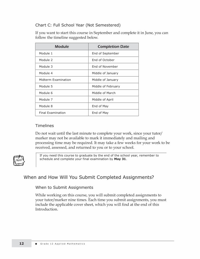
Chart C: Full School Year (Not Semestered)
If you want to start this course in September and complete it in June, you can follow the timeline suggested below.
Module Completion Date
Module 1 End of September
Module 2 End of October
Module 3 End of November
Module 4 Middle of January
Midterm Examination Middle of January
Module 5 Middle of February
Module 6 Middle of March
Module 7 Middle of April
Module 8 End of May
Final Examination End of May
Timelines
Do not wait until the last minute to complete your work, since your tutor/marker may not be available to mark it immediately and mailing and processing time may be required. It may take a few weeks for your work to be received, assessed, and returned to you or to your school.
If you need this course to graduate by the end of the school year, remember to schedule and complete your final examination by May 31.
When and How Will You Submit Completed Assignments?
When to Submit Assignments
While working on this course, you will submit completed assignments to your tutor/marker nine times. Each time you submit assignments, you must include the applicable cover sheet, which you will find at the end of this Introduction.

I n t r o d u c t i o n 13
The following chart shows you exactly what assignments you will be submitting at the end of each module.
Submission of Assignments
Submission Assignments You Will Submit
1 Module 1: FunctionsModule 1 Cover SheetModule 1 Cover Assignment: Inky PuzzleAssignment 1.1: Polynomial FunctionsAssignment 1.2: Logarithmic Function
2 Module 2: Mathematics Research ProjectModule 2 Cover Sheet 1Module 2 Cover Assignment: The Tower of HanoiAssignment 2.1: Project Proposal
3 Module 2: Mathematics Research ProjectModule 2 Cover Sheet 2Assignment 2.2: Collecting and Assessing DataAssignment 2.3: Interpreting DataAssignment 2.4: Presentation
4 Module 3: Logical ReasoningModule 3 Cover SheetModule 3 Cover Assignment: Sets GameAssignment 3.1: Sets and Conditional Statements
5 Module 4: ProbabilityModule 4 Cover SheetModule 4 Cover Assignment: StrategiesAssignment 4.1: Probability and Odds
6 Module 5: Financial MathematicsModule 5 Cover SheetModule 5 Cover Assignment: Crossing the Canal with CatsAssignment 5.1: Compound InterestAssignment 5.2: Loans and InvestmentsAssignment 5.3: Investment Decisions
7 Module 6: Techniques of CountingModule 6 Cover SheetModule 6 Cover Assignment: Patterns in NumbersAssignment 6.1: Fundamental Counting PrincipleAssignment 6.2: Applications of Permutations and Combinations
8 Module 7: Sinusoidal FunctionsModule 7 Cover SheetModule 7 Cover Assignment: Playing FairAssignment 7.1: Sinusoidal Function Models
9 Module 8: Design and MeasurementModule 8 Cover SheetModule 8 Cover Assignment: Container ConundrumAssignment 8.1: Design and Cost DecisionsAssignment 8.2: Working within a Project Budget

G r a d e 1 2 A p p l i e d M a t h e m a t i c s14
How to Submit Assignments
In this course, you have the choice of submitting your assignments either by mail or electronically. QQ Mail: Each time you mail something, you must include the print version of
the applicable cover sheet (found at the end of this Introduction).QQ Electronic submission: Each time you submit something electronically,
you must include the electronic version of the applicable cover sheet (found in the Student Downloads section of the distance learning website at <www.edu.gov.mb.ca/k12/dl/downloads/index.html>) or you can scan the cover sheet located at the end of this Introduction.
Complete the information at the top of each cover sheet before submitting it along with your assignments.
Submitting Your Assignments by MailIf you choose to mail your completed assignments, please photocopy/scan all the materials first so that you will have a copy of your work in case your package goes missing. You will need to place the applicable module cover sheet and assignments in an envelope, and address it to ISO Tutor/Marker 555 Main Street Winkler MB R6W 1C4
Your tutor/marker will mark your work and return it to you by mail.
Submitting Your Assignments ElectronicallyAssignment submission options vary by course. Sometimes assignments can be submitted electronically and sometimes they must be submitted by mail. Specific instructions on how to submit assignments were sent to you with this course. You can also obtain this information in the Grading and Evaluation section of the distance learning website at <www.edu.gov.mb.ca/k12/dl/iso/assignments.html>.
If you are submitting assignments electronically, make sure you have saved copies of them before you send them. That way, you can refer to your assignments when you discuss them with your tutor/marker. Also, if the original assignments are lost, you are able to resubmit them.
Your tutor/marker will mark your work and return it to you electronically.
The Independent Study Option office does not provide technical support for hardware-related issues. If troubleshooting is required, consult a professional computer technician.

I n t r o d u c t i o n 15
What Are the Guide Graphics For?
Guide graphics are used throughout this course to identify and guide you in specific tasks. Each graphic has a specific purpose, as described below.
Lesson Introduction: The introduction sets the stage for the lesson. It may draw upon prior knowledge or briefly describe the organization of the lesson. It also lists the learning outcomes for the lesson. Learning outcomes describe what you will learn.
Learning Partner: Ask your learning partner to help you with this task.
Learning Activity: Complete a learning activity. This will help you to review or practise what you have learned and prepare you for an assignment or an examination. You will not submit learning activities to your tutor/marker. Instead, you will compare your responses to those provided in the Learning Activity Answer Key found at the end of the applicable module.
Assignment: Complete an assignment. You will submit your completed assignments to your tutor/marker for assessment at the end of a given module.
Mail or Electronic Submission: Mail or electronically submit your completed assignments to your tutor/marker for assessment.
Tutor/Marker: Contact your tutor/marker.
Resource Sheet: Indicates material that may be valuable to include on your resource sheet.
Examination: Write your midterm or final examination at this time.
Note: Take note of and remember this important information or reminder.

G r a d e 1 2 A p p l i e d M a t h e m a t i c s16
Getting Started
Take some time right now to skim through the course material, locate your cover sheets, and familiarize yourself with how the course is organized. Get ready to learn!
Remember: If you have questions or need help at any point during this course, contact your tutor/marker or ask your learning partner for help.
Good luck with the course!

G r a d e 1 2 a p p l i e d M a t h e M a t i c s (4 0 s )
Module 1 Functions


M o d u l e 1 : F u n c t i o n s
Introduction
Welcome to your first module of Grade 12 Applied Mathematics! You will begin with a look back at linear and quadratic functions, and then extend these concepts to include cubic, exponential, and logarithmic functions. You will analyze and describe the characteristics of these functions, and match their graphs to the correct equations. You will determine which function best approximates contextual data and use it to solve problems.
Assignments in Module 1
To obtain credit for Module 1, you will need to send the following three assignments to your tutor/marker when you have completed this module. Your evaluation for this module is based on these assignments.
Lesson Assignment Number Assignment Title
Cover Assignment Inky Puzzle
2 Assignment 1.1 Polynomial Functions
6 Assignment 1.2 Logarithmic Function Models
M o d u l e 1 : F u n c t i o n s 3
Resource Sheet
When you write your midterm examination, you are encouraged to take a Midterm Exam Resource Sheet with you into the examination. This sheet will be one letter-sized page, 8½ ‘’ by 11”, and can be either handwritten or typewritten. Both sides of the sheet may be filled. You will submit it with your examination, but you do not receive any marks for it.
Many students have found that preparing a resource sheet is an excellent way to review. It provides you with a summary of the important facts of each module. You should complete a resource sheet for each module to help with your studying and reviewing. Lesson summaries and module summaries are included for you to use as a guide.
You may use the list of instructions provided below to help you with preparing your resource sheet for the material in Module 1. On this sheet, you should record math terms and definitions, formulas, sample questions, or a list of places where you often make mistakes. You should also identify special areas that require extra attention or review by writing the page numbers.
After you have completed each module’s resource sheet, you may summarize the sheets from Modules 1 to 4 to prepare your Midterm Exam Resource Sheet. The midterm examination for this course is based on Modules 1 to 4.
Resource Sheet for Module 1
1. List all the important math terms, and define them if necessary.2. List all the formulas and perhaps a sample problem that shows how the
formula is used.3. If necessary, write the solutions to some problems, showing in detail how
you did the calculations.4. Copy any questions that represent the key points of the lesson, and perhaps
include the solutions as well.5. Identify the problems you found most difficult, and copy the page numbers
onto the resource sheet so that you can review them before writing the examination. You may also copy the problems and the solutions onto your resource sheet, and later write them onto your Midterm Exam Resource Sheet.
6. Write any comments, ideas, shortcuts, or other reminders that may be helpful during an examination.
G r a d e 1 2 A p p l i e d M a t h e m a t i c s4
M o d u l e 1 : F u n c t i o n s 9
l e s s o n 1 : c h a r a c t e r i s t i c s o F p o l y n o M i a l F u n c t i o n s
Lesson Focus
In this lesson, you willq describe the characteristics of polynomial functions by analyzing
their graphs and equationsq match polynomial equations in a set to their corresponding
graphs
Lesson Introduction
Polynomial functions can be used to describe many real-world applications, including the pathway of a football tossed into the end zone during a Grey Cup game, the revenue generated from the drama club’s ticket sales as the price increases, and the relationship between the surface area and volume of an open box.
Polynomial Functions
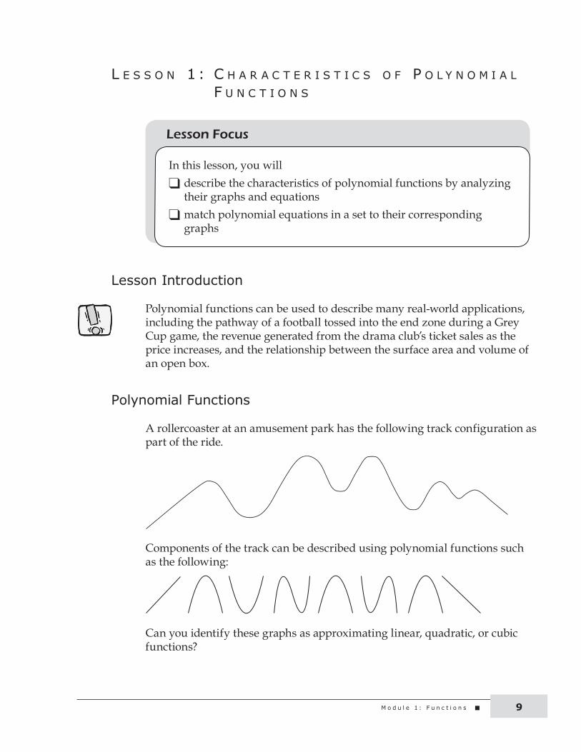
A rollercoaster at an amusement park has the following track configuration as part of the ride.
Components of the track can be described using polynomial functions such as the following:
Can you identify these graphs as approximating linear, quadratic, or cubic functions?

G r a d e 1 2 A p p l i e d M a t h e m a t i c s10
In previous math courses, you studied linear functions (Grade 10) and quadratic functions (Grade 11). In this lesson, you will extend your knowledge of polynomial functions to include cubic functions.
Recall that a polynomial function in one variable is made up of terms consisting of a variable with whole number exponents and real number coefficients, separated by addition or subtraction signs. Terms are written in descending order of power and the polynomial is named by its degree. The degree of a polynomial function is the greatest exponent of the function.
Degree Name Example
0 Constant f(x) = 2
1 Linear f(x) = x + 2
2 Quadratic f(x) = x2 - 5x + 6
3 Cubic f(x) = x3 - 4x2 + 2x - 6
4 Quartic f(x) = -3x4 + x
5 Quintic f(x) = 5x5 + 4x3 - 6
Polynomials with a degree higher than 5 are named by their degree. For example, f(x) = 2x8 + 6x7 - x5 + 3x4 + 5x2 - 19 would be called an eighth degree polynomial. This course will consider polynomial functions with degree of 3 or less.
Technology Requirements
You must have access to graphing technology for this course. There are many possible and appropriate types of software and hardware available, such as graphing calculators, mobile apps, websites, or free graphing programs. Some programs and/or apps can be found by searching or using the urls shown below: QQ WinPlot <http://math.exeter.edu/rparris/winplot.html>QQ Geogebra <www.geogebra.org/cms/>QQ Graphmatica <http://download.cnet.com/Graphmatica/3000-2053_4-10031384.
html>QQ Meta-Calculator <www.meta-calculator.com/online/> (mobile version is
available on the App Store)QQ Desmos <www.desmos.com>

M o d u l e 1 : F u n c t i o n s 11
The technology you choose to use for this module must have the capability to plot data, display graphs, determine the equation of the line or curve of best fit that best describes it, and analyze the data. You may need to try different applications as you complete the assignments in this course. It is your responsibility to learn how to use your chosen technology in order to fulfill the requirements of this course. Read the manual or help file that comes with it or find online tutorials to help you learn how to input equations, adjust the window settings, and view and analyze graphs. When submitting your work for marking, you may need to record your calculator keystrokes, print the screen shots or the graphs you create, or make sketches of the final image in your notes.
You are required to use technology to complete some parts of this module. Although you may use a variety of apps as you work on the content of this module, you will be asked when submitting assignments and on the day of the midterm examination to specify one graphing app or graphing technology that you are using for your assessment of the course.
Please see the Technology Appendix for further information on how to use certain technology applications to fulfill the requirements of this course.
The Graphs of Polynomial Functions
In order to identify and describe the characteristics of polynomial functions, it is helpful to graph them with a continuous curve on a Cartesian grid.
Recall that a Cartesian grid is divided by the x- and y-axes into four quadrants. They are named using roman numerals starting from the top right quadrant and progressing counter-clockwise.
�
�
��
��
�
�
�
�����
���
�����

G r a d e 1 2 A p p l i e d M a t h e m a t i c s12
Linear Functions
�
�
��
��
�
�
�
�����
���
��� ��
�������
�������
The graph of a linear function is a straight line.
Unless the line is horizontal or vertical, each line has one x-intercept (where y = 0) and one y-intercept (where x = 0).
The domain of each function is {x|x Î Â} and the range is {y|y Î Â}.
The end behaviour of a function is a description of the shape of the graph, read from left to right, as the value of x continues from negative infinity to positive infinity. The line of Graph A is always increasing and extends from Quadrant III to Quadrant I. The line of Graph B is always decreasing and extends from Quadrant II to Quadrant IV.
Quadratic Functions
�
�
��
��
�
�
�
�����
�������
�������
The graph of a quadratic function is a parabola. The line may have two, one, or zero x-intercepts. Recall that x-intercepts may also be called zeros and they are the roots of a related equation. The line will have one y-intercept.

M o d u l e 1 : F u n c t i o n s 13
The end behaviour of the line either extends from Quadrant II to Quadrant I, or from Quadrant III to Quadrant IV, depending on whether the graph opens up (cup shape) or opens down (hill shape).
Quadratic functions have either a maximum or a minimum y-value. At this turning point or vertex, the line has a smooth curve as the function changes from increasing to decreasing (maximum) or from decreasing to increasing (minimum).
The domain of each function is {x|x Î Â} and the range is either {y|y £ maximum, y Î Â} or {y|y ³ minimum, y Î Â}.
This information may be useful to add to your resource sheet for future reference.
Cubic Functions
�
�
� �����
��
��
�
�
�
�
� �����
��
��
�
�
�
�
� �
��
��
���� �
�
�
�
� �����
��
��
�
�
� �
� �
����������������
����������������
����������������
����������������
����������������
����������������

G r a d e 1 2 A p p l i e d M a t h e m a t i c s14
The shape of a cubic function graph is a smooth line with either zero or two turning points (where the function changes between increasing and decreasing). The graph may have one, two, or three x-intercepts and will have one y-intercept.
The end behaviour of the curve is either to extend from Quadrant III to Quadrant I or from Quadrant II to Quadrant IV.
There are no absolute maximum or minimum values in the curve as the line extends to both positive and negative infinity. The domain of each function is {x|x Î Â} and the range is {y|y Î Â}. In a given interval, however, the line may have a peak or valley. These smooth curved turning points are called either a relative maximum or a relative minimum (that is, maximum or minimum relative to the points on the function in the immediate vicinity).
The first cubic function, graph A above, does not have any turning points. Instead, it flattens out and crosses the x-axis without switching between increasing and decreasing. Graphs B, C, and D have two turning points, so they have both a relative maximum and a relative minimum.
Analyzing the Equations of Polynomial Functions
You have seen how the degree of a polynomial function determines the shape of the graph. The characteristics of each graph are connected to the coefficients and the constant in the equation for each function.
The equations of polynomial functions can be written in general form as follows:
Linear: f(x) = ax + b, where a ¹ 0
Quadratic: f(x) = ax2 + bx + c, where a ¹ 0
Cubic: f(x) = ax3 + bx2 + cx + d, where a ¹ 0
The terms are written in descending order of powers. The coefficient of the highest power, a, is called the leading coefficient.

M o d u l e 1 : F u n c t i o n s 15
Impact of the Constant and Coefficients in Polynomial Functions
Explore the impact of changing the value of the constant and the sign of the leading coefficient in the equations of polynomial functions.
Example 1What happens when the value of the constant is changed? Using your choice of technology, graph each set of polynomial functions on a grid, and compare the lines and equations.
Set 1: Set 2: Set 3:
f x x f x xf x xf x x
( ) = + ( ) =
( ) = +
( ) = −
055
or
f x x x
f x x x
f x x x
f x x x
( ) = +
( ) = + −
( ) = + +
( ) = + +
2
2
2
2
6
6 5
6 5
6 10
f x x x x
f x x x x
f x x x x
( ) = + +
( ) = + + +
( ) = + + −
3 2
3 2
3 2
5 4
5 4 5
5 4 5
SolutionSet 1:
�
�
�
�
�
�
�
�
��
������ ��
��
��
��
�
�
������������
������������
��������
The lines are parallel.
G r a d e 1 2 A p p l i e d M a t h e m a t i c s16
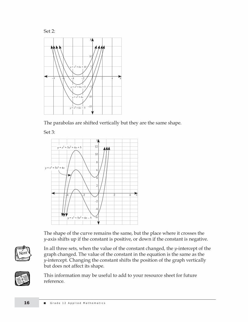
Set 2:
�
�
����������
��
�
���
��
������������������
�����������
���������������
����������������
The parabolas are shifted vertically but they are the same shape.
Set 3:�
�
�
�
�
�
��
��
��
��
��
���� � �
���������������������
���������������������
������������������
The shape of the curve remains the same, but the place where it crosses the y-axis shifts up if the constant is positive, or down if the constant is negative.
In all three sets, when the value of the constant changed, the y-intercept of the graph changed. The value of the constant in the equation is the same as the y-intercept. Changing the constant shifts the position of the graph vertically but does not affect its shape.
This information may be useful to add to your resource sheet for future reference.

M o d u l e 1 : F u n c t i o n s 17
Example 2What happens when the sign of the leading coefficient is changed? Graph each set of polynomial functions on a grid and compare the lines and equations.
Set 1: Set 2: Set 3:
f x xf x x
( ) =
( ) =−
f x x
f x x
( ) =
( ) =−
2
2
f x x
f x x
( ) =
( ) =−
3
3
SolutionSet 1:
��� ���
�
��
�
��
�
�
���������
��������
The slope of the line changes from positive to negative.
Set 2:
��� ���
�
��
�
��
�
����������
����������
The direction of opening switches from concave up (cup or valley shaped) to concave down (hill shaped).

G r a d e 1 2 A p p l i e d M a t h e m a t i c s18
Set 3:
��� ���
�
��
�
��
�
��������������������
Instead of rising to the right, the line falls to the right. The end behaviour is opposite.
In all three sets of graphs, when the sign of the leading coefficient changed, the end behaviour of the line was altered. If the line extended from Quadrant III to Quadrant I, it switched to Quadrant II to Quadrant IV. If the curve extended from Quadrant II to Quadrant I, it switched to Quadrant III to Quadrant IV. When the sign of the leading coefficient changes, the graph is reflected in the x-axis.
This information may be useful to add to your resource sheet for future reference.
Using the Equation to Identify Characteristics of a Polynomial Function
The characteristics of a polynomial function can be described without graphing it by considering the values of the constant and coefficients in the equation.
Example 1Without graphing the equation, determine the characteristics of the following functions.
a)
b)
c)
f x x x
g x x x x
h x x x x
( ) =− + +
( ) = − − −
( ) = −( ) +( ) −(
3 14 8
2 2
1 1 2
2
3 2
))

M o d u l e 1 : F u n c t i o n s 19
Solution
a) f x x x( ) =− + +3 14 82
This is a quadratic polynomial of degree 2, so it will have one turning point. Since the leading coefficient is negative, the parabola will open down. It will have an absolute maximum. The end behaviour of the curve will extend from Quadrant III to Quadrant IV. The y-intercept is at 8 (let x = 0). Since this is a positive value, the vertex must be above the x-axis. Therefore, the line will cross the x-axis twice. The domain of the function is {x|x Î Â} and the range is {y|y £ maximum, y Î Â}.
b) g x x x x( ) = − − −3 22 2
This is a third degree or cubic function. Just from looking at the general form, it is hard to determine the exact shape. It could have zero or two turning points and one, two, or three x-intercepts. It has a y-intercept at -2, the value of the constant (let x = 0). It has a positive leading term so the end behaviour of the line will extend from Quadrant III to Quadrant I. The domain of the function is {x|x Î Â} and the range is {y|y Î Â}, so there is no absolute maximum or minimum, but there would be a relative maximum and minimum if the line has turning points.
c) h x x x x( ) = −( ) +( ) −( )1 1 2
This function is not written in general form, but even in its factored form, it still represents a cubic function of degree 3. If the distributive property were applied and the terms written in descending order of power, it would have a positive leading coefficient (coefficient of each x is +1), so the end behaviour would be from Quadrant III to Quadrant I. It has a y-intercept of +2 (let x = 0 and multiply values from each bracket). From the factored form, you can identify the three x-intercepts or zeros of the function as -1, +1, and +2. It must, therefore, have two turning points, a relative maximum, and a relative minimum.

G r a d e 1 2 A p p l i e d M a t h e m a t i c s20
Matching Polynomial Graphs and Equations
Using what you know about polynomial equations and the graphs of the functions, you can match the graphs and equations.
Example 1Consider the characteristics of the following equations and graphs and match the ones that represent the same function.
�
�
�
�
� �����
��
��
�
�
�
�
�
� �����
��
��
�
�
�
�
�
� �����
��
��
�
�
�
�
�
� �����
��
��
�
b x x x
h x x x
k x x
t x x
m x x x
( ) = − +
( ) =− + −
( ) = +
( ) =− +
( ) = −
3 3 4
3 214
2
3 4
2
3
3
2
3 2 −− −x 2

M o d u l e 1 : F u n c t i o n s 21
SolutionGraph A is a cubic function so it must be degree 3. The end behaviour indicates that it has a negative leading coefficient, because it extends from Quadrant II to Quadrant IV. The y-intercept is -2, so the constant must be -2. This graph represents the function h(x) = -x3 + 3x - 2.
Graph B is also a cubic function with a y-intercept of –2, but the leading coefficient must be positive as the line extends from Quadrant III to Quadrant I. This graph represents the function m(x) = x3 - 2x2 - x - 2.
Graph C is a parabola, so the equation must be degree 2. It opens down, so the leading coefficient must be negative. The y-intercept is 4, so the constant must be 4. This graph represents the function t(x) = -3x2 + 4.
Graph D is linear, a first degree polynomial. The slope and leading coefficient must be positive, and the constant must be 2. This graph represents the
function k x x( ) = +14
2.
Example 2Sketch a graph that matches each of the following sets of characteristics and justify your reasoning.a) Extends from Quadrant III to Quadrant I, two x-interceptsb) Two turning points, y-intercept at -5, relative minimum in Quadrant III.
SolutionThere are a variety of graphs that would satisfy these conditions.a) A curve with two x-intercepts could be quadratic
or cubic, but for the end behaviour to extend from Quadrant III to Quadrant I, it must be a cubic polynomial with a positive leading coefficient. The curve must cross the x-axis once and be tangent (bounce) once. The y-intercept may be positive or negative. Two possible curves with these characteristics are shown on the left.
b) Two turning points implies a cubic function. A relative minimum in Quadrant III means the end behaviour must extend from Quadrant II to Quadrant IV. The line must cross the y-axis at -5. A possible graph may look similar to the one on the left.
�
�
��
�
�

G r a d e 1 2 A p p l i e d M a t h e m a t i c s22
Learning Activity 1.1
Complete the following, and check your answers in the learning activity answer keys found at the end of this module.
Part A: BrainPower
The BrainPower questions are provided as a warm-up activity for your brain before trying the questions in Part B. Try to complete each question quickly, without the use of a calculator and without writing many steps on paper.1. Factor: x2 - 7x + 10
2. State the roots of the following quadratic function: f(x) = x2 + 5x + 6
3. The vertex of a quadratic function is at (-5, 31). State the equation of the axis of symmetry.
Complete the following, based on the graph below.
��� ���
�
��
�
��
�
�
4. State the domain.
5. State the range.
6. State the coordinates of the vertex.
7. State the value of the x-intercepts.
8. State the value of x at the y-intercept.
continued

M o d u l e 1 : F u n c t i o n s 23
Learning Activity 1.1 (continued)
Part B: Characteristics of Polynomial Functions
Remember, these questions are similar to the ones that will be on your assignments and midterm examination. So, if you were able to answer them correctly, you are likely to do well on your assignments and midterm examination. If you did not answer them correctly, you need to go back to the lesson and learn the necessary concepts.
1. Given the following graphs of polynomial functions, complete the chart with the required information.
�
�
�
�
� �
��
�� �
�
�
�
�
�
�
��
�
��
� �����
�
��
�
��
� �����
�
��
�
��
� �����
��
��
���
� � �� ��
�� ��
�� ��
continued

G r a d e 1 2 A p p l i e d M a t h e m a t i c s24
Learning Activity 1.1 (continued)
Graph A B C D
Type of Function
Degree
# of x-intercept(s)
# of y-intercept(s)
End behaviour
Absolute or relative maximum or minimum
Domain
Range
2. What is the connection between the degree of a function and the maximum possible number of x-intercepts?
3. What is the connection between the degree of a function and the maximum possible number of turning points?
4. Will a polynomial function always have a y-intercept?
5. How is the end behaviour of a function related to it having an odd or even degree?
6. Use a sketch to show how changing the value of the constant in a cubic equation can affect the number of x-intercepts it has.
continued

M o d u l e 1 : F u n c t i o n s 25
Learning Activity 1.1 (continued)
7. Match each of the following graphs with the equation that describes it.a)
�
�
�
�
� �
��
��
����
b)
�
�
� �
��
����
�
�
��
c)
�
�
� �
��
����
�
�
��
d)
�
�
�
��
��
�
�
��
� �����
e)
�
�
�
��
��
�
�
��
� �����
f)
�
�
�
��
��
�
�
��
� �����
�
____ ____ .
____ ____
f x x m x x x x
g x x x t x
( ) = ( ) = + − −( )( ) = + − (
3 3 2
2
0 3 2 5 6
2 )) = +
( ) =− + + + ( )=− − +
x
h x x x x w x x x
2
2 2 23 2 2____ ____continued

G r a d e 1 2 A p p l i e d M a t h e m a t i c s26
Learning Activity 1.1 (continued)
8. Match a polynomial function description to one of the numbered graphs. There are some descriptions that will match with more than one graph, but in the end each graph should be matched to a different description.a)
�
�
��
�
�
� �
��
��
��
b)
�
�
�
�
�
��
�� �
��
��
c)
�
�
�
�
�� ����
��
��
��
�
� � �
d)
�
�
�
��
��
�
�
� �
e)
�
�
�
�� �� �
�
��
��
��
��
f)
�
�� �� �
�
��
��
��
��
�
�
continued

M o d u l e 1 : F u n c t i o n s 27
Learning Activity 1.1 (continued)
g)
�
�� ��
�
��
��
��
�
�
�
h)
�
�� ��
�
��
��
��
�
�
�
i)
�
�� ��
�
��
��
�
�
�
��
� � �
j)
��� ��
�
��
��
�
� �
�
�
��
k)
��� ��
�
��
��
�
� �
��
�
�
l)
��� ��
�
��
��
�
� �
��
�
�
continued
G r a d e 1 2 A p p l i e d M a t h e m a t i c s28
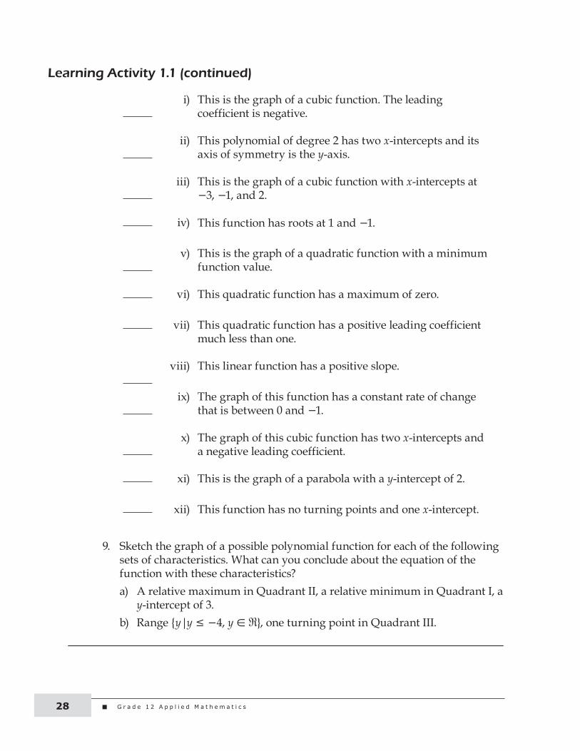
Learning Activity 1.1 (continued)
i) This is the graph of a cubic function. The leading coefficient is negative.
ii) This polynomial of degree 2 has two x-intercepts and its axis of symmetry is the y-axis.
iii) This is the graph of a cubic function with x-intercepts at -3, -1, and 2.
iv) This function has roots at 1 and -1.
v) This is the graph of a quadratic function with a minimum function value.
vi) This quadratic function has a maximum of zero.
vii) This quadratic function has a positive leading coefficient much less than one.
viii) This linear function has a positive slope.
ix) The graph of this function has a constant rate of change that is between 0 and -1.
x) The graph of this cubic function has two x-intercepts and a negative leading coefficient.
xi) This is the graph of a parabola with a y-intercept of 2.
xii) This function has no turning points and one x-intercept.
9. Sketch the graph of a possible polynomial function for each of the following sets of characteristics. What can you conclude about the equation of the function with these characteristics?a) A relative maximum in Quadrant II, a relative minimum in Quadrant I, a
y-intercept of 3.b) Range {y|y £ -4, y Î Â}, one turning point in Quadrant III.

M o d u l e 1 : F u n c t i o n s 29
Lesson Summary
In this lesson, you reviewed, analyzed, and described the characteristics of different types of polynomial graphs and equations. You considered the degree, domain and range, maximum and minimum values, x- and y-intercepts, turning points and end behaviour of graphs, and the constants and leading coefficients in equations. You sketched polynomial graphs and matched them to equations.

G r a d e 1 2 A p p l i e d M a t h e m a t i c s30
Notes


Printed in CanadaImprimé au Canada
Released 2015


![Applied Mathematics Introductory Module - PDST Maths Module [final].pdf · Applied Mathematics Introductory Module ... Science, Technology and ... ii. how to form mathematical models](https://img.dokumen.tips/doc/110x75/5af58cc37f8b9a4d4d8f3bdb/applied-mathematics-introductory-module-maths-module-finalpdfapplied-mathematics.jpg)