GOVST III, Paris Nov 2011 ECMWF ECMWF Report Magdalena Alonso Balmaseda Kristian Mogensen Operational Implementation of NEMO/NEMOVAR ORAS4: Ocean ReAnalysis

GOVST III, Paris Nov 2011 ECMWF

ECMWF Report

Magdalena Alonso BalmasedaKristian Mogensen

• Operational Implementation of NEMO/NEMOVAR

• ORAS4: Ocean ReAnalysis System 4

• Some lessons learnt during preparation

• Evaluation process

• Plans


Delayed Ocean Re-Analysis ~ORAS4 (NEMOVAR)

Real Time Ocean Analysis

ECMWF:

Forecasting Systems

ECMWF:

Forecasting Systems

Medium-Range (10-day)Partial coupling

Medium-Range (10-day)Partial coupling

Seasonal ForecastsFully coupled

Seasonal ForecastsFully coupled

Extended + Monthly Fully coupled

Extended + Monthly Fully coupled

Ocean model

Atmospheric model

Wave model

Atmospheric model

Ocean model

Wave model

Oce

an Init

ial

Condit

ions


• ECMWF has a implemented new operational ocean re-analysis system.

http://www.ecmwf.int/products/forecasts/d/charts/oras4/reanalysis/

• It implies the transition to NEMO/NEMOVAR from HOPE/OI

• It consists of 5 ensemble members, covering the period 1958-Present, continuously updated.

• It is used for the initialization of the operational monthly and seasonal forecasts.

• It is also used to initialize the CMIP5 decadal forecasts (EC-Earth …)

• It is a valuable resource for climate variability studies.

• Documentation in preparation: Mogensen et al 2011, Balmaseda et al 2011

ECMWF: Operational Ocean Changes in 2011. ORAS4

http://www.ecmwf.int/products/forecasts/d/charts/oras4/reanalysis/


Ocean Model: NEMO V3.0 ORCA1 and 42 levels (ocean)

Data Assimilation: NEMOVAR (3D-var FGAT).

Data: Temperature and Salinity Profiles (EN3-XBT corrected and GTS), SST (HADISST/ OIv21x1 /OSTIA), along track Altimeter Sea Level (AVISO). See figure below

Forcing: ERA40/ERA-INTERIM/ECMWF NWP (see figure below)

Bias Correction: In T/S and P gradient. Seasonal prescribed (from Argo+Alti) + Adaptive on line

Ensemble Generation: wind perturbations, observation coverage, spin-up. 5 ensemble members

ORAS4 Main Ingredients


What have we learned in the preparation process?

• Which SST product to use?• Which products are available? Criteria for evaluation

• Assimilation of altimeter: variational implementation of Cooper and Haines in 3Dvar. Non trivial. Sorted.

• Coastal Covariances: Impact of Assimilation in the Atlantic MOC.

• Bias correction scheme: estimation of the offline term from Argo period. (Not a problem, a success; It affects the results)

• How to evaluate ocean reanalyses?


Which SST product to use?

Options for Re-analysisOIV2_1x1: (weekly)~1982 onwardsOIV2_025_AVHRR(daily)~1982 onwardsOIV2_O25_AVHR+AMSR:~2002 onwardsOptions for Real-Time: As before +OSTIA (from 2008 onwards): Consistency with atmospheric analysis

OIV2_025_AVHRR: bias cold in the global mean (regional differences)

Bias decreases with time. OSTIA in beween (not shown)

Weaker interannual variability

Fit to insitu Temperature: bias cold in tropics, better in mid latitudes,.

Not clear impact on Seasonal Forecasts

DECISION: OIV2_1x1 until 2010, OSTIA thereafter.


Multivariate balance for AltimeterIN NEMOVAR the balance is between sea level and steric height

(1) )( :form lincrementain or ,00

zrefzref

dzzdz

Original formulation of NEMOVAR

αref and βref are calculated by linearizing the equation of estate using the background T/S values as reference. Comments:

i) zref=1500m is arbitrary. An attempt to take into account that baroclinicity is low below this level. Can we account for the vertical stratification more universally?

ii) this can lead to increments in model levels with large dz

SandT

STmz

refref

refref

refref

ref

(2) 1500


anom GLOBAL

1994 1996 1998 2000 2002 2004 2006 2008Time

0.00

0.02

0.04

0.06

0.08

0.10

0.12

AVISOCONTROLAssim: TSAltimeter+MDTcontrol

But Impact on Steric Height not realistic:

This problem not so apparent if assimilating T/S and

altimeter, but it is still there. Why?

SO10 _T3_P50_L320_Z0_V1:bckintSO10 _T3_P50_L320_Z0_V1:bckint

latitudes in [49.0, 51.0] - (4 points) (): Min= 1.3e-12, Max= 1.7e-02, Int= 1.0e-03

80W 60W 40W 20W 0ELongitude

50004000300020001000300250200150100500

Depth

(m

)

0.00 0.00 0.00 0.01 0.01 0.01 0.01 0.01 0.02 0.02




50004000300020001000300250200150100500

Depth

(m

)

0.00 0.00 0.00 0.01 0.01 0.01 0.01 0.01 0.02 0.02


latitudes in [49.0, 51.0] - (4 points) (): Min= 0.0e+00, Max= 1.6e-02, Int= 1.0e-03


50004000300020001000300250200150100500

Depth

(m

)

0.00 0.00 0.00 0.01 0.01 0.01 0.01 0.01 0.02 0.02




50004000300020001000300250200150100500

Depth

(m

)

0.00 0.00 0.00 0.01 0.01 0.01 0.01 0.01 0.02 0.02




50004000300020001000300250200150100500

Depth

(m

)

0.00 0.00 0.00 0.01 0.01 0.01 0.01 0.01 0.02 0.02

Single Obs Experiments: T increment

The temperature increment is applied to the thickest model

levels


Modifications

A):Weighting based on stratification. Use BV frequency to calculate αN and βN instead of equation of state

B) Do not double-count balance-salinity corrections

2 2 2 2;

z zN N z N T N S

z T S

2

2

ref ref ref ref

ref ref

T S S TN

z z T z

z S T zN T T

T T z T


anom GLOBAL

1994 1996 1998 2000 2002 2004 2006 2008Time

0.00

0.02

0.04

0.06

0.08

0.10

0.12

AVISOCONTROLAssim: TSAltimeter+MDTcontrol

New Balance formulation:

anom GLOBAL

1994 1996 1998 2000 2002 2004 2006 2008Time

0.00

0.01

0.02

0.03

0.04

AVISOCONTROLAssim:TSAlti+MDTcontrol(Modified)Sea Level Altimeter (AVISO)

CONTROLASSIM: TS

CONTROL+ALTIASSIM: TS + ALTI

Problem with Steric Height Solved

Problem with deep T increments Solved




50004000300020001000300250200150100500

Depth

(m

)

0.00 0.00 0.00 0.01 0.01 0.01 0.01 0.01 0.02 0.02




50004000300020001000300250200150100500

Depth

(m

)

0.00 0.00 0.00 0.01 0.01 0.01 0.01 0.01 0.02 0.02




50004000300020001000300250200150100500

Depth

(m

)

0.00 0.00 0.00 0.01 0.01 0.01 0.01 0.01 0.02 0.02




50004000300020001000300250200150100500

Depth

(m

)

0.00 0.00 0.00 0.01 0.01 0.01 0.01 0.01 0.02 0.02




50004000300020001000300250200150100500

Depth

(m

)

0.00 0.00 0.00 0.01 0.01 0.01 0.01 0.01 0.02 0.02

Old New

anom GLOBAL

1994 1996 1998 2000 2002 2004 2006 2008Time

0.00

0.01

0.02

0.03

0.04

AVISOCONTROLAssim:TSAlti+MDTcontrol(Modified)TS+Alti


rms EQ2 Potential Temperature

0.0 0.5 1.0 1.5 2.0 2.5rms EQ2 Potential Temperature

-500

-400

-300

-200

-100

0

Depth

(m

)

rms EQIND Potential Temperature

0.0 0.5 1.0 1.5 2.0rms EQIND Potential Temperature

-500

-400

-300

-200

-100

0

Depth

(m

)

rms TRPAC Potential Temperature

0.4 0.6 0.8 1.0 1.2 1.4rms TRPAC Potential Temperature

-500

-400

-300

-200

-100

0

Depth

(m

)

rms GLOBAL Potential Temperature

0.6 0.8 1.0 1.2 1.4 1.6rms GLOBAL Potential Temperature

-500

-400

-300

-200

-100

0

Depth

(m

)

CONTROL ASSIM: T+S ASSIM: T+S+Alti

EQ Central Pacific EQ Indian Ocean

TROPICAL Pacific GLOBAL

Altimeter Improves the fit to InSitu Temperature Data

RMSE of 10 days forecast


Assessment of the ORA-S4 re-analysis

Choose a baseline: the CONTROL (e.i., no data assim)

1. Assim Intrinsic Metrics

• Fit to obs (first-guess minus obs): Bias, RMS

• Error growth (An-obs versus FG-obs)

• Consistency: Prescribed/Diagnosed B and R

This is insufficient to assess a Reanalysis product

2. Spatial/temporal consistency: long time series and spatial maps

• Time correlation with Mooring currents

• Correlation with altimeter/Oscar currents

• Transports (MOC and RAPID): short time series

Quite limited records. Not always independent data

3. Skill of Seasonal Forecasts

Expensive. Model error can be a problem.

4. Observing System Experiments


Assimilation Statistics: Incremental Analysis Update

GLOBAL RMSE Temperature

0.4 0.6 0.8 1.0 1.2-1000

-800

-600

-400

-200

0

Dep

th (m

)

RMSE ANRMSE FGRMSE MIN


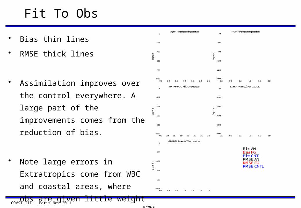
Fit To Obs

• Bias thin lines

• RMSE thick lines

• Assimilation improves over the

control everywhere. A large part

of the improvements comes

from the reduction of bias.

• Note large errors in Extratropics

come from WBC and coastal

areas, where obs are given little

weight

EQUA Potential Temperature

-0.5 0.0 0.5 1.0 1.5 2.0 2.5-1000

-800

-600

-400

-200

0

Depth

(m

)

TROP Potential Temperature

-0.5 0.0 0.5 1.0 1.5 2.0-1000

-800

-600

-400

-200

0

Depth

(m

)

NXTRP Potential Temperature

-0.5 0.0 0.5 1.0 1.5 2.0 2.5 3.0-1000

-800

-600

-400

-200

0

Depth

(m

)

SXTRP Potential Temperature

-0.5 0.0 0.5 1.0 1.5 2.0-1000

-800

-600

-400

-200

0

Depth

(m

)

GLOBAL Potential Temperature

-0.5 0.0 0.5 1.0 1.5 2.0 2.5-1000

-800

-600

-400

-200

0

Depth

(m

)

0.0 0.2 0.4 0.6 0.8 1.00.0

0.2

0.4

0.6

0.8

1.0

Bias ANBias FGBias CNTLRMSE ANRMSE FGRMSE CNTL


TROP Potential Temperature Depth= 200.0 meters

1960 1970 1980 1990 2000 2010Time

0.0

0.5

1.0

1.5

2.0Bias ORAS4

Bias CNTLRMSE ORAS4

RMSE CNTL

TROP Salinity Depth= 200.0 meters

1960 1970 1980 1990 2000 2010Time

0.00

0.05

0.10

0.15

0.20

0.25

0.30Bias ORAS4

Bias CNTLRMSE ORAS4

RMSE CNTL

Fit to Obs

ORAS4 shows reduced RMSE and bias respect the CNTL, in both T and S

The bias is ORAS4 is more stable in time

Fit improves with time, both ORAS4 and CNTL :Not only more subsurface obs, but better surface forcing and SST data?.


Fit to ADCP mooring data

• Some improvement of the Pacific and Atlantic undercurrents, which are still on the weak side.

T0N165E

-0.5 0.0 0.5 1.0Zonal current (m/s)

-300

-200

-100

0

Dep

th (m

)

T0N170W


-300

-200

-100

0

Dep

th (m

)

T0N140W


-300

-200

-100

0

Dep

th (m

)

P0N23W


-300

-200

-100

0

Dep

th (m

)

R0N90E


-300

-200

-100

0

Dep

th (m

)

R0N90E


-300

-200

-100

0

Dep

th (m

)

ADCP

ORAS4CNTL


NEMOVAR re-an: verif. against altimeter data

correl (1): fe5x sossheig ( 1993-2008 ) correl (1): fe5x sossheig ( 1993-2008 )

(ndim): Min= -0.37, Max= 1.00, Int= 0.02

100E 160W 60WLongitude

60S

40S

20S

0

20N

40N

60N

Latitud

e

0.40 0.44 0.48 0.52 0.56 0.60 0.64 0.68 0.72 0.76 0.80 0.84 0.88 0.92 0.96 1.00

RMSE (1): fe5x sossheig (1993-2008) RMSE (1): fe5x sossheig (1993-2008)

(m): Min= 0.01, Max= 0.15, Int= 0.01


60S

40S

20S

0

20N

40N

60N

Latitud

e

0.02 0.04 0.06 0.08 0.10

rms/signal(1): fe5x sossheig (1993-2008) rms/signal(1): fe5x sossheig (1993-2008)

(N/A): Min= 0.10, Max= 3.18, Int= 0.20


60S

40S

20S

0

20N

40N

60N

Latitud

e

0.00 0.40 0.80 1.20 1.60 2.00

sdv_fe5x/sdv_aviso (1): sossheig (1993-2008) sdv_fe5x/sdv_aviso (1): sossheig (1993-2008)

(N/A): Min= 0.22, Max= 2.74, Int= 0.20


60S

40S

20S

0

20N

40N

60N

Latitud

e

0.00 0.40 0.80 1.20 1.60 2.00

fa9p_oref_19932008_1_sossheig_stats.ps) Aug 4 2010

NEMOVAR T+S

ORA-S4: NEMOVAR T+S+Alti

CNTL NEMO NoObs


Comparison with RAPID derived transports

MOC

2002 2004 2006 2008 2010 20120

10

20

30Ekman

2002 2004 2006 2008 2010 2012-10

-5

0

5

10

MOC-Ekman

2002 2004 2006 2008 2010 20120

10

20

30ORAS4RAPID

Atlantic MOC at 26N

Short time seriesORAS4 underestimates the MOCNote the large minima in 2010 and 2011!!


More MOC diagnostics

MOC

1960 1970 1980 1990 2000 2010 20200

10

20

30MidOcean

1960 1970 1980 1990 2000 2010 2020-40

-30

-20

-10

0

Ekman

1960 1970 1980 1990 2000 2010 2020-10

-5

0

5

10

RAPIDCNTLORAS4

FST

1960 1970 1980 1990 2000 2010 202010

20

30

40

RAPIDORAS4CNTL

• In low res model the Florida Strait transport is not so well defined.

• Assimilation reduction of the FST is proportional to the weight is given to the obs (not shown)

• Ocean model tends to produce too strong and shallow AABW cell

MOC profile


Impact on Of ORAS4 in SST Seasonal ForecastsAnomaly correlation: ORAS4 CNTL Persistence


ERA+

ASMER

A ASM

-6

-4

-2

0

2

4

6

GLOBAL HEAT BUDGET

1960 1970 1980 1990 2000Time

-10

-5

0

5

10 ERA+ASM 0.23 W/m2ERA 4.99 W/m2ASM -4.76 W/m2

El ChichonPinatubo

Global Surface Heat Fluxes from Reanalysis


Meridional Heat Transport ATL 195801:200912Meridional Heat Transport ATL 195801:200912

20S 0 20N 40N 60N0.0

0.2

0.4

0.6

0.8

1.0

1.2

1.4

Meridional Heat Transport ATL 195801:200912

ORA-S4GW2000

Meridional Heat Transport INP0 195801:200912Meridional Heat Transport INP0 195801:200912

20S 0 20N 40N 60N-2.0

-1.5

-1.0

-0.5

0.0

0.5

1.0

1.5Meridional Heat Transport INP0 195801:200912

ORA-S4GW2000

Meridional Heat Transport GLO 195801:200912Meridional Heat Transport GLO 195801:200912

20S 0 20N 40N 60N-2

-1

0

1

2

3Meridional Heat Transport GLO 195801:200912

ORA-S4GW2000

drag) Oct 18 2011

Mean and time variability of ORAS4 oceanic heat transport.

(GW2000: Ganachaud and Wunsch 2000)

ORAS4 HEAT contributions (1.e22 J)

1970 1980 1990 2000Time

-5

0

5

10

15

Ocean Heat content 0.00Total=Surface+Relax+Assim+BiasC+Geothermal 5050.99ERA+ASSIM heat flux integral

ORAS4 total (whole depth) heat content

The time integral of the ERA+ASM surface heat flux

results in the evolution of the total ocean heat content

Climate Applications


Summary

• Operational implementation of NEMO/NEMOVAR in forecasting systems and ocean reanalysis • Transition from HOPE/OI• ORAS4: new Ocean Reanalysis with NEMOVAR• Still climate resolution: approx 1x1 degree.

• Some lessons learns in the preparation process• Choice of SST product for reanalysis not trivial. Next is to try OSTIA reanalysis• Balance relationship between altimeter and T/S not solved problem. Not trivial. Still room for

improvement• Improved covariance needed for the assimilation of observations near the coast.

• How to evaluate an ocean assimilation system and ocean reanalyses product?

• Evaluation of the ocean reanalysis is a pre-requisite for the interpretation of climate signals• Standard assimilation statistics needed but not sufficient for the reanalyses• Need information about time variability: sustained time series are very important:

(altimeter, moorings, RAPID, other?)• Impact on seasonal forecast is a test and a result.

• What is next?• Document system, web pages, papers• Higher resolution ocean model and reanalysis(ORCA 025)• Sea-Ice model in monthly, seasonal forecast and reanalyses• Improved coupling (bulk formula, wave effects, ocean mixed layer)• Increased coupling (forecast and analysis)

Documents

GOVST III, Paris Nov 2011 ECMWF ECMWF Report Magdalena Alonso Balmaseda Kristian Mogensen Operational Implementation of NEMO/NEMOVAR ORAS4: Ocean ReAnalysis